Embed Size (px)
Citation preview

HAL Id: inria-00590273https://hal.inria.fr/inria-00590273v2
Submitted on 10 Aug 2011
HAL is a multi-disciplinary open accessarchive for the deposit and dissemination of sci-entific research documents, whether they are pub-lished or not. The documents may come fromteaching and research institutions in France orabroad, or from public or private research centers.
L’archive ouverte pluridisciplinaire HAL, estdestinée au dépôt et à la diffusion de documentsscientifiques de niveau recherche, publiés ou non,émanant des établissements d’enseignement et derecherche français ou étrangers, des laboratoirespublics ou privés.
3D Shape Registration Using Spectral GraphEmbedding and Probabilistic Matching
Avinash Sharma, Radu Horaud, Diana Mateus
To cite this version:Avinash Sharma, Radu Horaud, Diana Mateus. 3D Shape Registration Using Spectral Graph Embed-ding and Probabilistic Matching. Olivier Lezoray and Leo Grady. Image Processing and AnalysingWith Graphs: Theory and Practice, CRC Press, pp.441-474, 2012. �inria-00590273v2�

Chapter 8
3D Shape Registration Using Spectral
Graph Embedding and Probabilistic
MatchingAVINASH SHARMA
INRIA Grenoble Rhone-Alpes655 avenue de l’Europe38330 Montbonnot Saint-Martin, [email protected]
RADU HORAUD
INRIA Grenoble Rhone-Alpes655 avenue de l’Europe38330 Montbonnot Saint-Martin, [email protected]
DIANA MATEUS
Institut fur InformatikTechnische Universitat MunchenGarching b. Munchen [email protected]

2 Image Processing and Analysing Graphs: Theory and Practice
Abstract
In this book chapter we address the problem of 3D shape registration and we propose a novel technique
based on spectral graph theory and probabilistic matching. Recent advancement in shape acquisition tech-
nology has led to the capture of large amounts of 3D data. Existing real-time multi-camera 3D acquisition
methods provide a frame-wise reliable visual-hull or mesh representations for real 3D animation sequences
The task of 3D shape analysis involves tracking, recognition, registration, etc. Analyzing 3D data in a single
framework is still a challenging task considering the large variability of the data gathered with different ac-
quisition devices. 3D shape registration is one such challenging shape analysis task. The main contribution
of this chapter is to extend the spectral graph matching methods to very large graphs by combining spectral
graph matching with Laplacian embedding. Since the embedded representation of a graph is obtained by
dimensionality reduction we claim that the existing spectral-based methods are not easily applicable. We
discuss solutions for the exact and inexact graph isomorphism problems and recall the main spectral proper-
ties of the combinatorial graph Laplacian; We provide a novel analysis of the commute-time embedding that
allows us to interpret the latter in terms of the PCA of a graph, and to select the appropriate dimension of
the associated embedded metric space; We derive a unit hyper-sphere normalization for the commute-time
embedding that allows us to register two shapes with different samplings; We propose a novel method to find
the eigenvalue-eigenvector ordering and the eigenvector sign using the eigensignature (histogram) which is
invariant to the isometric shape deformations and fits well in the spectral graph matching framework, and
we present a probabilistic shape matching formulation using an expectation maximization point registration
algorithm which alternates between aligning the eigenbases and finding a vertex-to-vertex assignment.
8.1 Introduction
In this chapter we discuss the problem of 3D shape registration. Recent advancement in shape acquisition
technology has led to the capture of large amounts of 3D data. Existing real-time multi-camera 3D ac-
quisition methods provide a frame-wise reliable visual-hull or mesh representations for real 3D animation
sequences [1, 2, 3, 4, 5, 6]. The task of 3D shape analysis involves tracking, recognition, registration,
etc. Analyzing 3D data in a single framework is still a challenging task considering the large variability of
the data gathered with different acquisition devices. 3D shape registration is one such challenging shape
analysis task. The major difficulties in shape registration arise due to: 1) variation in the shape acquisi-
tion techniques, 2) local deformations in non-rigid shapes, 3) large acquisition discrepancies (e.g., holes,
topology change, surface acquisition noise), 4) local scale change.
Most of the previous attempts of shape matching can be broadly categorized as extrinsic or intrinsic

3D Shape Registration Using Spectral Graph Embedding and Probabilistic Matching 3
approaches depending on how they analyze the properties of the underlying manifold. Extrinsic approaches
mainly focus on finding a global or local rigid transformation between two 3D shapes.
There is large set of approaches based on variations of Iterative Closest Point (ICP) algorithm [?, ?, 7]
that falls in the category of extrinsic approaches. However, the majority of these approaches compute rigid
transformations for shape registration and are not directly applicable to non-rigid shapes. Intrinsic ap-
proaches are a natural choice for finding dense correspondences between articulated shapes, as they em-
bed the shape in some canonical domain which preserves some important properties of the manifold, e.g.,
geodesics and angles. Intrinsic approaches are preferable over extrinsic as they provide a global representa-
tion which is invariant to non-rigid deformations that are common in the real-world 3D shapes.
Interestingly, mesh representation also enables the adaptation of well established graph matching algo-
rithms that use eigenvalues and eigenvectors of graph matrices, and are theoretically well investigated in the
framework of Spectral Graph Theory (SGT) e.g., [8, 9]. Existing methods in SGT are mainly theoretical
results applied to small graphs and under the premise that eigenvalues can be computed exactly. However,
spectral graph matching does not easily generalize to very large graphs due to the following reasons: 1)
eigenvalues are approximately computed using eigen-solvers, 2) eigenvalue multiplicity and hence ordering
change are not well studied, 3) exact matching is intractable for very large graphs. It is important to note
that these methods mainly focus on exact graph matching while majority of the real-world graph matching
applications involve graphs with different cardinality and for which only a subgraph isomorphism can be
sought.
The main contribution of this work is to extend the spectral graph methods to very large graphs by
combining spectral graph matching with Laplacian Embedding. Since the embedded representation of a
graph is obtained by dimensionality reduction we claim that the existing SGT methods (e.g., [8]) are not
easily applicable. The major contributions of this work are the following: 1) we discuss solutions for the
exact and inexact graph isomorphism problems and recall the main spectral properties of the combinatorial
graph Laplacian, 2) we provide a novel analysis of the commute-time embedding that allows us to interpret
the latter in terms of the PCA of a graph, and to select the appropriate dimension of the associated embedded
metric space, 3) we derive a unit hyper-sphere normalization for the commute-time embedding that allows
us to register two shapes with different samplings, 4) we propose a novel method to find the eigenvalue-
eigenvector ordering and the eigenvector signs using the eigensignatures (histograms) that are invariant to
the isometric shape deformations and which fits well in the spectral graph matching framework, 5) we
present a probabilistic shape matching formulation using expectation maximization for point registration
algorithm which alternates between aligning the eigenbases and finding a vertex-to-vertex assignment.
The existing graph matching methods that use intrinsic representations are: [10, 11, 12, 13, 14, 15,

4 Image Processing and Analysing Graphs: Theory and Practice
Figure 8.1: Overview of the proposed method. First, a Laplacian embedding is obtained for each shape.
Next, these embeddings are aligned to handle the issue of sign flip and ordering change using the histogram
matching. Finally, an Expectation-Maximization based point registration is performed to obtain dense prob-
abilistic matching between two shapes.
16, 17]. There is another class of methods that allows to combine intrinsic (geodesics) and extrinsic (ap-
pearance) features and which were previously successfully applied for matching features in pairs of images
[?, ?, ?, 19, 20, 21, 22, 23, 24, 25]. Some recent approaches apply hierarchical matching to find dense
correspondences [26, 27, 28]. However, many of these graph matching algorithms suffer from the problem
of either computational intractability or a lack of proper distance metric (w.r.t. underlying manifold struc-
ture) as the Euclidean metric is not directly applicable while computing distances on non-rigid shapes. A
recent benchmarking of shape matching methods was performed in [29]. Recently, a few methods proposed
a diffusion framework for the task of shape registration [30, 31, 32].
In this chapter we present an intrinsic approach for unsupervised 3D shape registration first proposed
in [14, 33]. In the first step, dimensionality reduction is performed using the graph Laplacian which allows
us to embed a 3D shape in an isometric subspace invariant to non-rigid deformations. This leads to an
embedded point cloud representation where each vertex of the underlying graph is mapped to a point in
a K-dimensional metric space. Thus, the problem of non-rigid 3D shape registration is transformed into
a K-dimensional point registration task. However, before point registration, the two eigen spaces need to
be correctly aligned. This alignment is critical for the spectral matching methods because the two eigen
spaces are defined up to the signs and the ordering of the eigenvectors of their Laplacian matrices. This
is achieved by a novel matching method that uses histograms of eigenvectors as eigensignatures. In the
final step, a point registration method based on a variant of the expectation-maximization (EM) algorithm
[34] is applied in order to register two sets of points associated with the Laplacian embeddings of the two
shapes. The proposed algorithm alternates between the estimation of an orthogonal transformation matrix
associated with the alignment of the two eigen spaces and the computation of probabilistic vertex-to-vertex
assignment. Figure 1.1 presents the overview of the proposed method. According to the results summarized
in [29], this method is one among the best performing unsupervised shape matching algorithms.

3D Shape Registration Using Spectral Graph Embedding and Probabilistic Matching 5
Chapter Overview: Graph matrices are introduced in section 1.2. The problem of exact graph isomor-
phism and existing solutions are discussed in section 1.3. Section 1.4 deals with dimensionality reduction
using the graph Laplacian in order to obtain embedded representations for 3D shapes. In the same section
we discuss the PCA of graph embeddings and propose a unit hyper-sphere normalization for these embed-
dings along with a method to choose the embedding dimension. Section 1.5 introduces the formulation of
maximum subgraph isomorphism before presenting a two-step method for 3D shape registration. In the
first step Laplacian embeddings are aligned using histogram matching while in the second step we briefly
discuss an EM point registration method to obtain probabilistic shape registration. Finally we present shape
matching results in section 1.6 and conclude with a brief discussion in section 1.7.
8.2 Graph Matrices
A shape can be treated as a connected undirected weighted graph G = {V,E} where V(G) = {v1, . . . ,vn} is
the vertex set, E(G) = {ei j} is the edge set. Let W be the weighted adjacency matrix of this graph. Each
(i, j)th entry of W matrix stores weight wi j whenever there is an edge ei j ∈ E(G) between graph vertices vi
and v j and 0 otherwise with all the diagonal elements set to 0 . We use the following notations: The degree
di of a graph vertex di = ∑i∼ j wi j (i ∼ j denotes the set of vertices v j which are adjacent to vi), the degree
matrix D = diag[d1 . . .di . . .dn], the n×1 vector 1= (1 . . .1)> (the constant vector), the n×1 degree vector
d = D1, and the graph volume Vol(G) = ∑i di.
In spectral graph theory, it is common [35, 36] to use the following expression for the edge weights:
wi j = e−dist2(vi ,v j)
σ2 , (8.1)
where dist(vi,v j) denotes any distance metric between two vertices and σ is a free parameter. In the case of
a fully connected graph, matrix W is also referred to as the similarity matrix. The normalized weighted ad-
jacency matrix writes W = D−1/2WD−1/2. The transition matrix of the non-symmetric reversible Markov
chain associated with the graph is WR = D−1W = D−1/2WD1/2.
8.2.1 Variants of the Graph Laplacian Matrix
We can now build the concept of the graph Laplacian operator. We consider the following variants of the
Laplacian matrix [37, 36, 38]:
• The unnormalized Laplacian which is also referred to as the combinatorial Laplacian L,
• the normalized Laplacian L, and

6 Image Processing and Analysing Graphs: Theory and Practice
• the random-walk Laplacian LR also referred to as the discrete Laplace operator.
In more detail we have:
L = D−W (8.2)
L = D−1/2LD−1/2 = I−W (8.3)
LR = D−1L = I−WR (8.4)
with the following relations between these matrices:
L = D1/2LD1/2 = DLR (8.5)
L = D−1/2LD−1/2 = D1/2LRD−1/2 (8.6)
LR = D−1/2LD1/2 = D−1L. (8.7)
8.3 Spectral Graph Isomorphism
Let GA and GB be two undirected weighted graphs with the same number of nodes, n, and let WA and WB
be their adjacency matrices. They are real-symmetric matrices. In the general case, the number r of distinct
eigenvalues of these matrices is smaller than n. The standard spectral methods only apply to those graphs
whose adjacency matrices have n distinct eigenvalues (each eigenvalue has multiplicity one), which implies
that the eigenvalues can be ordered.
Graph isomorphism [39] can be written as the following minimization problem:
P? = argminP‖WA−PWBP>‖2
F (8.8)
where P is an n×n permutation matrix (see appendix A.1) with P? as the desired vertex-to-vertex permuta-
tion matrix and ‖•‖F is the Frobenius norm defined by (see appendix A.2):
‖W‖2F = 〈W,W〉=
n
∑i=1
n
∑j=1
w2i j = tr(W>W) (8.9)
Let:
WA = UAΛAU>A (8.10)
WB = UBΛBU>B (8.11)
be the eigen-decompositions of the two matrices with n eigenvalues ΛA = diag[αi] and ΛB = diag[βi] and n
orthonormal eigenvectors, the column vectors of UA and UB.

3D Shape Registration Using Spectral Graph Embedding and Probabilistic Matching 7
8.3.1 An Exact Spectral Solution
If there exists a vertex-to-vertex correspondence that makes (1.8) equal to 0, we have:
WA = P?WBP?>. (8.12)
This implies that the adjacency matrices of the two graphs should have the same eigenvalues. Moreover,
if the eigenvalues are non null and, the matrices UA and UB have full rank and are uniquely defined by their
n orthonormal column vectors (which are the eigenvectors of WA and WB), then αi = βi,∀i, 1≤ i≤ n and
ΛA = ΛB. From (1.12) and using the eigen-decompositions of the two graph matrices we obtain:
ΛA = U>A P?UBΛBU>B P?>UA = ΛB, (8.13)
where the matrix UB is defined by:
UB = UBS. (8.14)
Matrix S = diag[si], with si =±1, is referred to as a sign matrix with the property S2 = I. Post multiplication
of UB with a sign matrix takes into account the fact that the eigenvectors (the column vectors of UB) are
only defined up to a sign. Finally we obtain the following permutation matrix:
P? = UBSU>A . (8.15)
Therefore, one may notice that there are as many solutions as the cardinality of the set of matrices Sn, i.e.,
|Sn|= 2n, and that not all of these solutions correspond to a permutation matrix. This means that there exist
some matrices S? that exactly make P? a permutation matrix. Hence, all those permutation matrices that
satisfy (1.15) are solutions of the exact graph isomorphism problem. Notice that once the permutation has
been estimated, one can write that the rows of UB can be aligned with the rows of UA:
UA = P?UBS?. (8.16)
The rows of UA and of UB can be interpreted as isometric embeddings of the two graph vertices: A vertex
vi of GA has as coordinates the ith row of UA. This means that the spectral graph isomorphism problem
becomes a point registration problem, where graph vertices are represented by points in Rn. To conclude,
the exact graph isomorphism problem has a spectral solution based on: (i) the eigen-decomposition of the
two graph matrices, (ii) the ordering of their eigenvalues, and (iii) the choice of a sign for each eigenvector.
8.3.2 The Hoffman-Wielandt Theorem
The Hoffman-Wielandt theorem [40, 41] is the fundamental building block of spectral graph isomorphism.
The theorem holds for normal matrices; Here, we restrict the analysis to real symmetric matrices, although
the generalization to Hermitian matrices is straightforward:

8 Image Processing and Analysing Graphs: Theory and Practice
Theorem 1
(Hoffman and Wielandt) If WA and WB are real-symmetric matrices, and if αi and βi are their eigenvalues
arranged in increasing order, α1 ≤ . . .≤ αi ≤ . . .≤ αn and β1 ≤ . . .≤ βi ≤ . . .≤ βn, then
n
∑i=1
(αi−βi)2 ≤ ‖WA−WB‖2F . (8.17)
Proof: The proof is derived from [9, 42]. Consider the eigen-decompositions of matrices WA and WB,
(1.10), (1.11). Notice that for the time being we are free to prescribe the ordering of the eigenvalues αi and
βi and hence the ordering of the column vectors of matrices UA and UB. By combining (1.10) and (1.11) we
write:
UAΛAU>A −UBΛBU>B = WA−WB (8.18)
or, equivalently:
ΛAU>A UB−U>A UBΛB = U>A (WA−WB)UB. (8.19)
By the unitary-invariance of the Frobenius norm (see appendix A.2 ) and with the notation Z = U>A UB we
obtain:
‖ΛAZ−ZΛB‖2F = ‖WA−WB‖2
F , (8.20)
which is equivalent to:n
∑i=1
n
∑j=1
(αi−β j)2z2i j = ‖WA−WB‖2
F . (8.21)
The coefficients xi j = z2i j can be viewed as the entries of a doubly-stochastic matrix X: xi j ≥ 0,∑n
i=1 xi j =
1,∑nj=1 xi j = 1. Using these properties, we obtain:
n
∑i=1
n
∑j=1
(αi−β j)2z2i j =
n
∑i=1
α2i +
n
∑j=1
β2j −2
n
∑i=1
n
∑j=1
z2i jαiβ j
≥n
∑i=1
α2i +
n
∑j=1
β2j −2max
Z
{n
∑i=1
n
∑j=1
z2i jαiβ j
}. (8.22)
Hence, the minimization of (1.21) is equivalent to the maximization of the last term in (1.22). We
can modify our maximization problem to admit all the doubly-stochastic matrices. In this way we seek an
extremum over a convex compact set. The maximum over this compact set is larger than or equal to our
maximum:
maxZ∈On
{n
∑i=1
n
∑j=1
z2i jαiβ j
}≤ max
X∈Dn
{n
∑i=1
n
∑j=1
xi jαiβ j
}(8.23)
where On is the set of orthogonal matrices and Dn is the set of doubly stochastic matrices (see appendix A.1).
Let ci j = αiβ j and hence one can write that the right term in the equation above as the dot-product of two
matrices:
〈X,C〉= tr(XC) =n
∑i=1
n
∑j=1
xi jci j. (8.24)

3D Shape Registration Using Spectral Graph Embedding and Probabilistic Matching 9
Figure 8.2: This figure illustrates the maximization of the dot-product 〈X,C〉. The two matrices can be
viewed as vectors of dimension n2. Matrix X belongs to a compact convex set whose extreme points are
the permutation matrices P1,P2, . . . ,Pn. Therefore, the projection of this set (i.e., Dn) onto C has projected
permutation matrices at its extremes, namely 〈Pmin,X〉 and 〈Pmax,X〉 in this example.
Therefore, this expression can be interpreted as the projection of X onto C, see figure 1.2. The Birkhoff
theorem (appendix A.1) tells us that the set Dn of doubly stochastic matrices is a compact convex set. We
obtain that the extrema (minimum and maximum) of the projection of X onto C occur at the projections
of one of the extreme points of this convex set, which correspond to permutation matrices. Hence, the
maximum of 〈X,C〉 is 〈Pmax,X〉 and we obtain:
maxX∈Dn
{n
∑i=1
n
∑j=1
xi jαiβ j
}=
n
∑i=1
αiβπ(i). (8.25)
By substitution in (1.22) we obtain:
n
∑i=1
n
∑j=1
(αi−β j)2z2i j ≥
n
∑i=1
(αi−βπ(i))2. (8.26)
If the eigenvalues are in increasing order then the permutation that satisfies theorem 1.17 is the identity
matrix, i.e., π(i) = i. Indeed, let’s assume that for some indices k and k + 1 we have: π(k) = k + 1 and
π(k +1) = k. Since αk ≤ αk+1 and βk ≤ βk+1, the following inequality holds:
(αk−βk)2 +(αk+1−βk+1)2 ≤ (αk−βk+1)2 +(αk+1−βk)2 (8.27)
and hence (1.17) holds. �

10 Image Processing and Analysing Graphs: Theory and Practice
Corollary 1.1
The inequality (1.17) becomes an equality when the eigenvectors of WA are aligned with the eigenvectors
of WB up to a sign ambiguity:
UB = UAS. (8.28)
Proof: Since the minimum of (1.21) is achieved for X = I and since the entries of X are z2i j, we have
that zii =±1, which corresponds to Z = S. �
Corollary 1.2
If Q is an orthogonal matrix, then
n
∑i=1
(αi−βi)2 ≤ ‖WA−QWBQ>‖2F . (8.29)
Proof: Since the eigen-decomposition of matrix QWBQ> is (QUB)ΛB(QUB)> and since it has the
same eigenvalues as WB, the inequality (1.29) holds and hence corollary 1.2. �
These corollaries will be useful in the case of spectral graph matching methods presented below.
8.3.3 Umeyama’s Method
The exact spectral matching solution presented in section 1.3.1 finds a permutation matrix satisfying (1.15).
This requires an exhaustive search over the space of all possible 2n matrices. Umeyama’s method presented
in [8] proposes a relaxed solution to this problem as outlined below.
Umeyama [8] addresses the problem of weighted graph matching within the framework of spectral
graph theory. He proposes two methods, the first for undirected weighted graphs and the second for directed
weighted graphs. The adjacency matrix is used in both cases. Let’s consider the case of undirected graphs.
The eigenvalues are (possibly with multiplicities):
WA : α1 ≤ . . .≤ αi ≤ . . .≤ αn (8.30)
WB : β1 ≤ . . .≤ βi ≤ . . .≤ βn. (8.31)
Theorem 2
(Umeyama) If WA and WB are real-symmetric matrices with n distinct eigenvalues (that can be ordered),
α1 < .. . < αi < .. . < αn and β1 < .. . < βi < .. . < βn, the minimum of :
J(Q) = ‖WA−QWBQ>‖2F (8.32)

3D Shape Registration Using Spectral Graph Embedding and Probabilistic Matching 11
is achieved for:
Q? = UASU>B (8.33)
and hence (1.29) becomes an equality:n
∑i=1
(αi−βi)2 = ‖WA−Q?WBQ?>‖2F . (8.34)
Proof: The proof is straightforward. By corollary 1.2, the Hoffman-Wielandt theorem applies to
matrices WA and QWBQ>. By corollary 1.1, the equality (1.34) is achieved for:
Z = U>A Q?UB = S (8.35)
and hence (1.33) holds. �
Notice that (1.33) can be written as:
UA = Q?UBS (8.36)
which is a relaxed version of (1.16): The permutation matrix in the exact isomorphism case is replaced by
an orthogonal matrix.
A Heuristic for Spectral Graph Matching: Let us consider again the exact solution outlined in sec-
tion 1.3.1. Umeyama suggests a heuristic in order to avoid exhaustive search over all possible 2n matrices
that satisfy (1.15). One may easily notice that:
‖P−UASU>B ‖2F = 2n−2tr(UAS(PUB)>). (8.37)
Using Umeyama’s notations, UA = [|ui j|],UB = [|vi j|] (the entries of UA are the absolute values of the entries
of UA), one may further notice that:
tr(UAS(PUB)>) =n
∑i=1
n
∑j=1
s jui jvπ(i) j ≤n
∑i=1
n
∑j=1|ui j||vπ(i) j|= tr(UAU
>B P>). (8.38)
The minimization of (1.37) is equivalent to the maximization of (1.38) and the maximal value that can
be attained by the latter is n. Using the fact that both UA and UB are orthogonal matrices, one can easily
conclude that:
tr(UAU>B P>)≤ n. (8.39)
Umeyama concludes that when the two graphs are isomorphic, the optimum permutation matrix maximizes
tr(UAU>B P>) and this can be solved by the Hungarian algorithm [43].
When the two graphs are not exactly isomorphic, theorem 1 and theorem 2 allow us to relax the permu-
tation matrices to the group of orthogonal matrices. Therefore with similar arguments as above we obtain:
tr(UASU>B Q>)≤ tr(UAU>B Q>)≤ n. (8.40)

12 Image Processing and Analysing Graphs: Theory and Practice
The permutation matrix obtained with the Hungarian algorithm can be used as an initial solution that can
then be improved by some hill-climbing or relaxation technique [8].
The spectral matching solution presented in this section is not directly applicable to large graphs. In the
next section we introduce the notion of dimensionality reduction for graphs which will lead to a tractable
graph matching solution.
8.4 Graph Embedding and Dimensionality Reduction
For large and sparse graphs, the results of section 1.3 and Umeyama’s method (section 1.3.3) hold only
weakly. Indeed, one cannot guarantee that all the eigenvalues have multiplicity equal to one: the presence of
symmetries causes some of eigenvalues to have an algebraic multiplicity greater than one. Under these cir-
cumstances and due to numerical approximations, it might not be possible to properly order the eigenvalues.
Moreover, for very large graphs with thousands of vertices it is not practical to compute all its eigenvalue-
eigenvector pairs. This means that one has to devise a method that is able to match shapes using a small set
of eigenvalues and eigenvectors.
One elegant way to overcome this problem, is to reduce the dimension of the eigenspace, along the
line of spectral dimensionality reductions techniques. The eigendecomposition of graph Laplacian matrices
(introduced in section 1.2.1) is a popular choice for the purpose of dimensionality reduction [35].
8.4.1 Spectral Properties of the Graph Laplacian
The spectral properties of the Laplacian matrices introduced in section 1.2.1 have been thoroughly studied.
They are summarized in table 1.1. We derive some subtle properties of the combinatorial Laplacian which
Laplacian Null space Eigenvalues Eigenvectors
L = UΛU> u1 = 1 0 = λ1 < λ2 ≤ . . .≤ λn u>i>11= 0,u>i u j = δi j
L = UΓU>
u1 = D1/21 0 = γ1 < γ2 ≤ . . .≤ γn u>i>1D1/2
1= 0, u>i u j = δi j
LR = TΓT−1, T = D−1/2U t1 = 1 0 = γ1 < γ2 ≤ . . .≤ γn t>i>1D1= 0,t>i Dt j = δi j
Table 8.1: Summary of the spectral properties of the Laplacian matrices. Assuming a connected graph, the
null eigenvalue (λ1,γ1) has multiplicity one. The first non null eigenvalue (λ2,γ2) is known as the Fiedler
value and its multiplicity is, in general, equal to one. The associated eigenvector is denoted the Fiedler
vector [37].
will be useful for the task of shape registration. In particular, we will show that the eigenvectors of the

3D Shape Registration Using Spectral Graph Embedding and Probabilistic Matching 13
combinatorial Laplacian can be interpreted as directions of maximum variance (principal components) of
the associated embedded shape representation. We note that the embeddings of the normalized and random-
walk Laplacians have different spectral properties which make them less interesting for shape registration,
i.e., Appendix A.3.
The combinatorial Laplacian. Let L = UΛU> be the spectral decomposition of the combinatorial Lapla-
cian with UU> = I. Let U be written as:
U =
u11 . . . u1k . . . u1n
......
...
un1 . . . unk . . . unn
(8.41)
Each column of U, uk = (u1k . . .uik . . .unk)> is an eigenvector associated with the eigenvalue λk. From the
definition of L in (1.2) (see [35]) one can easily see that λ1 = 0 and that u1 = 1 (a constant vector). Hence,
u>k≥21= 0 and by combining this with u>k uk = 1, we derive the following proposition:
Proposition 1
The components of the non-constant eigenvectors of the combinatorial Laplacian satisfy the following con-
straints:
∑ni=1 uik = 0, ∀k,2≤ k ≤ n (8.42)
−1 < uik < 1, ∀i,k,1≤ i≤ n,2≤ k ≤ n. (8.43)
Assuming a connected graph, λ1 has multiplicity equal to one [36]. Let’s organize the eigenvalues of L in
increasing order: 0 = λ1 < λ2 ≤ . . .≤ λn. We prove the following proposition [37]:
Proposition 2
For all k ≤ n, we have λk ≤ 2maxi(di), where di is the degree of vertex i.
Proof: The largest eigenvalue of L corresponds to the maximization of the Rayleigh quotient, or
λn = maxu
u>Lu
u>u. (8.44)
We have u>Lu = ∑ei j wi j(ui−u j)2. From the inequality (a−b)2 ≤ 2(a2 +b2) we obtain:
λn ≤2∑ei j wi j(u2
i +u2j)
∑i u2i
=2∑i diu2
i
∑i u2i≤ 2max
i(di). � (8.45)
14 Image Processing and Analysing Graphs: Theory and Practice
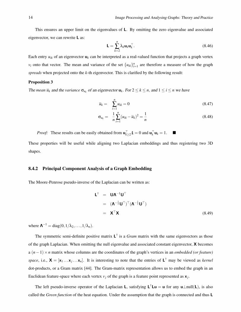
This ensures an upper limit on the eigenvalues of L. By omitting the zero eigenvalue and associated
eigenvector, we can rewrite L as:
L =n
∑k=2
λkuku>k . (8.46)
Each entry uik of an eigenvector uk can be interpreted as a real-valued function that projects a graph vertex
vi onto that vector. The mean and variance of the set {uik}ni=1 are therefore a measure of how the graph
spreads when projected onto the k-th eigenvector. This is clarified by the following result:
Proposition 3
The mean uk and the variance σuk of an eigenvector uk. For 2≤ k ≤ n, and 1≤ i≤ n we have
uk =n
∑i=1
uik = 0 (8.47)
σuk =1n
n
∑i=1
(uik−uk)2 =1n
(8.48)
Proof: These results can be easily obtained from u>k≥21= 0 and u>k uk = 1. �
These properties will be useful while aligning two Laplacian embeddings and thus registering two 3D
shapes.
8.4.2 Principal Component Analysis of a Graph Embedding
The Moore-Penrose pseudo-inverse of the Laplacian can be written as:
L† = UΛ−1U>
= (Λ−12 U>)>(Λ−
12 U>)
= X>X (8.49)
where Λ−1 = diag(0,1/λ2, . . . ,1/λn).
The symmetric semi-definite positive matrix L† is a Gram matrix with the same eigenvectors as those
of the graph Laplacian. When omitting the null eigenvalue and associated constant eigenvector, X becomes
a (n−1)×n matrix whose columns are the coordinates of the graph’s vertices in an embedded (or feature)
space, i.e., X = [x1 . . .x j . . .xn]. It is interesting to note that the entries of L† may be viewed as kernel
dot-products, or a Gram matrix [44]. The Gram-matrix representation allows us to embed the graph in an
Euclidean feature-space where each vertex v j of the graph is a feature point represented as x j.
The left pseudo-inverse operator of the Laplacian L, satisfying L†Lu = u for any u⊥null(L), is also
called the Green function of the heat equation. Under the assumption that the graph is connected and thus L

3D Shape Registration Using Spectral Graph Embedding and Probabilistic Matching 15
has an eigenvalue λ1 = 0 with multiplicity 1, we obtain:
L† =n
∑k=2
1λk
uku>k . (8.50)
The Green function is intimately related to random walks on graphs, and can be interpreted probabilistically
as follows. Given a Markov chain such that each graph vertex is the state, and the transition from vertex
vi is possible to any adjacent vertex v j ∼ vi with probability wi j/di, the expected number of steps required
to reach vertex v j from vi, called the access or hitting time O(vi,v j). The expected number of steps in
a round trip from vi to v j is called the commute-time distance: CTD2(vi,v j) = O(vi,v j) + O(v j,vi). The
commute-time distance [45] can be expressed in terms of the entries of L†:
CTD2(vi,v j) = Vol(G)(L†(i, i)+L†( j, j)−2L†(i, j))
= Vol(G)
(n
∑k=2
1λk
u2ik +
n
∑k=2
1λk
u2jk−2
n
∑k=2
1λk
uiku jk
)
= Vol(G)n
∑k=2
(λ−1/2k (uik−u jk)
)2
= Vol(G)‖xi−x j‖2, (8.51)
where the volume of the graph, Vol(G) is the sum of the degrees of all the graph vertices. The CTD func-
tion is positive-definite and sub-additive, thus defining a metric between the graph vertices, referred to as
commute-time (or resistance) distance [46]. The CTD is inversely related to the number and length of
paths connecting two vertices. Unlike the shortest-path (geodesic) distance, CTD captures the connectivity
structure of the graph volume rather than a single path between the two vertices. The great advantage of
the commute-time distance over the shortest geodesic path is that it is robust to topological changes and
therefore is well suited for characterizing complex shapes. Since the volume is a graph constant, we obtain:
CTD2(vi,v j) ∝ ‖xi−x j‖2. (8.52)
Hence, the Euclidean distance between any two feature points xi and x j is the commute time distance
between the graph vertex vi and v j.
Using the first K non-null eigenvalue-eigenvector pairs of the Laplacian L, the commute-time embedding
of the graph’s nodes corresponds to the column vectors of the K×n matrix X:
XK×n = Λ−1/2K (Un×K)> = [x1 . . .x j . . .xn]. (8.53)
From (1.43) and (1.53) one can easily infer lower and upper bounds for the i-th coordinate of x j:
−λ−1/2i < x ji < λ
−1/2i . (8.54)

16 Image Processing and Analysing Graphs: Theory and Practice
The last equation implies that the graph embedding stretches along the eigenvectors with a factor that is
inversely proportional to the square root of the eigenvalues. Theorem 3 below characterizes the smallest non-
null K eigenvalue-eigenvector pairs of L as the directions of maximum variance (the principal components)
of the commute-time embedding.
Theorem 3
The largest eigenvalue-eigenvector pairs of the pseudo-inverse of the combinatorial Laplacian matrix are
the principal components of the commute-time embedding, i.e., the points X are zero-centered and have a
diagonal covariance matrix.
Proof: Indeed, from (1.47) we obtain a zero-mean while from (1.53) we obtain a diagonal covariance
matrix:
x =1n
n
∑i=1
xi =1n
Λ−12
∑
ni=1 ui2
...
∑ni=1 uik+1
=
0...
0
(8.55)
ΣX =1n
XX> =1n
Λ−12 U>UΛ−
12 =
1n
Λ−1 (8.56)
�.
Figure 1.3 shows the projection of graph (in this case 3D shape represented as meshes) vertices on eigen-
vectors.
(a) (b) (c)
Figure 8.3: This is an illustration of the concept of the PCA of a graph embedding. The graph’s vertices are
projected onto the second, third and fourth eigenvectors of the Laplacian matrix. These eigenvectors can be
viewed as the principal directions of the shape.

3D Shape Registration Using Spectral Graph Embedding and Probabilistic Matching 17
8.4.3 Choosing the Dimension of the Embedding
A direct consequence of theorem 3 is that the embedded graph representation is centered and the eigenvec-
tors of the combinatorial Laplacian are the directions of maximum variance. The principal eigenvectors cor-
respond to the eigenvectors associated with the K largest eigenvalues of the L†, i.e., λ−12 ≥ λ
−13 ≥ . . .≥ λ
−1K .
The variance along vector uk is λ−1k /n. Therefore, the total variance can be computed from the trace of the
L† matrix :
tr(ΣX) =1n
tr(L†). (8.57)
A standard way of choosing the principal components is to use the scree diagram:
θ(K) =∑
K+1k=2 λ
−1k
∑nk=2 λ
−1k
. (8.58)
The selection of the first K principal eigenvectors therefore depends on the spectral fall-off of the inverses
of the eigenvalues. In spectral graph theory, the dimension K is chosen on the basis of the existence of
an eigengap, such that λK+2− λK+1 > t with t > 0. In practice it is extremely difficult to find such an
eigengap, in particular in the case of sparse graphs that correspond to a discretized manifold. Instead, we
propose to select the dimension of the embedding in the following way. Notice that (1.58) can be written
as θ(K) = A/(A + B) with A = ∑K+1k=2 λ
−1k and B = ∑
nk=K+2 λ
−1k . Moreover, from the fact that the λk’s are
arranged in increasing order, we obtain B≤ (n−K−1)λ−1K+1. Hence:
θmin ≤ θ(K)≤ 1, (8.59)
with
θmin =∑
K+1k=2 λ
−1k
∑Kk=2 λ
−1k +(n−K)λ−1
K+1. (8.60)
This lower bound can be computed from the K smallest non null eigenvalues of the combinatorial Laplacian
matrix. Hence, one can choose K such that the sum of the first K eigenvalues of the L† matrix is a good
approximation of the total variance, e.g., θmin = 0.95.
8.4.4 Unit Hyper-sphere Normalization
One disadvantage of the standard embeddings is that, when two shapes have large difference in sampling the
embeddings will differ by a significant scale factor. In order to avoid this we can normalize the embedding
such that the vertex coordinates lie on a unit sphere of dimension K, which yields:
xi =xi
‖xi‖. (8.61)
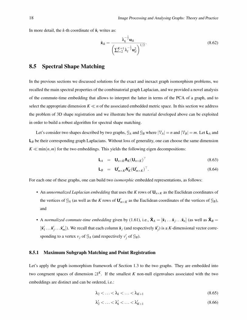
18 Image Processing and Analysing Graphs: Theory and Practice
In more detail, the k-th coordinate of xi writes as:
xik =λ− 1
2k uik(
∑K+1l=2 λ
− 12
l u2il
)1/2 . (8.62)
8.5 Spectral Shape Matching
In the previous sections we discussed solutions for the exact and inexact graph isomorphism problems, we
recalled the main spectral properties of the combinatorial graph Laplacian, and we provided a novel analysis
of the commute-time embedding that allows to interpret the latter in terms of the PCA of a graph, and to
select the appropriate dimension K� n of the associated embedded metric space. In this section we address
the problem of 3D shape registration and we illustrate how the material developed above can be exploited
in order to build a robust algorithm for spectral shape matching.
Let’s consider two shapes described by two graphs, GA and GB where |VA|= n and |VB|= m. Let LA and
LB be their corresponding graph Laplacians. Without loss of generality, one can choose the same dimension
K�min(n,m) for the two embeddings. This yields the following eigen decompositions:
LA = Un×KΛK(Un×K)> (8.63)
LB = U′m×KΛ′K(U′m×K)>. (8.64)
For each one of these graphs, one can build two isomorphic embedded representations, as follows:
• An unnormalized Laplacian embedding that uses the K rows of Un×K as the Euclidean coordinates of
the vertices of GA (as well as the K rows of U′m×K as the Euclidean coordinates of the vertices of GB),
and
• A normalized commute-time embedding given by (1.61), i.e., XA = [x1 . . . x j . . . xn] (as well as XB =
[x′1 . . . x′j . . . x′m]). We recall that each column x j (and respectively x′j) is a K-dimensional vector corre-
sponding to a vertex v j of GA (and respectively v′j of GB).
8.5.1 Maximum Subgraph Matching and Point Registration
Let’s apply the graph isomorphism framework of Section 1.3 to the two graphs. They are embedded into
two congruent spaces of dimension RK . If the smallest K non-null eigenvalues associated with the two
embeddings are distinct and can be ordered, i.e.:
λ2 < .. . < λk < .. . < λK+1 (8.65)
λ′2 < .. . < λ
′k < .. . < λ
′K+1 (8.66)

3D Shape Registration Using Spectral Graph Embedding and Probabilistic Matching 19
then, the Umeyama method could be applied. If one uses the unnormalized Laplacian embeddings just
defined, (1.33) becomes:
Q? = Un×KSK(U′m×K)> (8.67)
Notice that here the sign matrix S defined in 1.33 became a K×K matrix denoted by SK . We now
assume that the eigenvalues {λ2, . . . ,λK+1} and {λ′2, . . . ,λ′K+1} cannot be reliably ordered. This can be
modeled by multiplication with a K×K permutation matrix PK :
Q = Un×KSKPK(U′m×K)> (8.68)
Pre-multiplication of (U′m×K)> with PK permutes its rows such that u′k→ u′π(k). Each entry qi j of the n×m
matrix Q can therefore be written as:
qi j =K+1
∑k=2
skuiku′jπ(k) (8.69)
Since both Un×K and U′m×K are column-orthonormal matrices, the dot-product defined by (1.69) is equiva-
lent to the cosine of the angle between two K-dimensional vectors. This means that each entry of Q is such
that −1≤ qi j ≤+1 and that two vertices vi and v′j are matched if qi j is close to 1.
One can also use the normalized commute-time coordinates and define an equivalent expression as
above:
Q = X>
SKPKX′
(8.70)
with:
qi j =K+1
∑k=2
skxikx′jπ(k) (8.71)
Because both sets of points X and X′lie on a K-dimensional unit hyper-sphere, we also have−1≤ qi j ≤+1.
It should however be emphasized that the rank of the n×m matrices Q,Q is equal to K. Therefore,
these matrices cannot be viewed as relaxed permutation matrices between the two graphs. In fact they
define many-to-many correspondences between the vertices of the first graph and the vertices of the second
graph, this being due to the fact that the graphs are embedded on a low-dimensional space. This is one of
the main differences between our method proposed in the next section and the Umeyama method, as well
as many other subsequent methods, that use all eigenvectors of the graph. As it will be explained below,
our formulation leads to a shape matching method that will alternate between aligning their eigenbases and
finding a vertex-to-vertex assignment.
It is possible to extract a one-to-one assignment matrix from Q (or from Q) using either dynamic pro-
gramming or an assignment method technique such as the Hungarian algorithm. Notice that this assignment
is conditioned by the choice of a sign matrix SK and of a permutation matrix PK , i.e., 2KK! possibilities,

20 Image Processing and Analysing Graphs: Theory and Practice
and that not all these choices correspond to a valid sub-isomorphism between the two graphs. Let’s consider
the case of the normalized commute-time embedding; there is an equivalent formulation for the unnormal-
ized Laplacian embedding. The two graphs are described by two sets of points, X and X′, both lying onto
the K-dimensional unity hyper-sphere. The K×K matrix SKPK transforms one graph embedding onto the
other graph embedding. Hence, one can write xi = SKPK x′j if vertex vi matches v j. More generally Let
RK = SKPK and let’s extend the domain of RK to all possible orthogonal matrices of size K×K, namely
RK ∈ OK or the orthogonal group of dimension K. We can now write the following criterion whose min-
imization over RK guarantees an optimal solution for registering the vertices of the first graph with the
vertices of the second graph:
minRK
n
∑i=1
m
∑j=1
qi j‖xi−RK x′j‖2 (8.72)
One way to solve minimization problems such as (1.72) is to use a point registration algorithm that
alternates between (i) estimating the K×K orthogonal transformation RK , which aligns the K-dimensional
coordinates associated with the two embeddings, and (ii) updating the assignment variables qi j. This can be
done using either ICP-like methods (the qi j’s are binary variables), or EM-like methods (the qi j’s are poste-
rior probabilities of assignment variables). As we just outlined above, matrix RK belongs to the orthogonal
group OK . Therefore this framework differs from standard implementations of ICP and EM algorithms that
usually estimate a 2-D or 3-D rotation matrix which belong to the special orthogonal group.
It is well established that ICP algorithms are easily trapped in local minima. The EM algorithm recently
proposed in [34] is able to converge to a good solution starting with a rough initial guess and is robust to the
presence of outliers. Nevertheless, the algorithm proposed in [34] performs well under rigid transformations
(rotation and translation), whereas in our case we have to estimate a more general orthogonal transformation
that incorporates both rotations and reflections. Therefore, before describing in detail an EM algorithm
well suited for solving the problem at hand, we discuss the issue of estimating an initialization for the
transformation aligning the K eigenvectors of the first embedding with those of the second embedding and
we propose a practical method for initializing this transformation (namely, matrices SK and PK in (1.70))
based on comparing the histograms of these eigenvectors, or eigensignatures.
8.5.2 Aligning Two Embeddings Based on Eigensignatures
Both the unnormalized Laplacian embedding and the normalized commute-time embedding of a graph are
represented in a metric space spanned by the eigenvectors of the Laplacian matrix, namely the n-dimensional
vectors {u2, . . . ,uk, . . . ,uK+1}, where n is the number of graph vertices. They correspond to eigenfunc-
tions and each such eigenfunction maps the graph’s vertices onto the real line. More precisely, the k-th

3D Shape Registration Using Spectral Graph Embedding and Probabilistic Matching 21
eigenfunction maps a vertex vi onto uik. Propositions 1 and 3 revealed interesting statistics of the sets
{u1k, . . . ,uik, . . . ,unk}K+1k=2 . Moreover, theorem 3 provided an interpretation of the eigenvectors in terms of
principal directions of the embedded shape. One can therefore conclude that the probability distribution of
the components of an eigenvector have interesting properties that make them suitable for comparing two
shapes, namely −1 < uik < +1, uk = 1/n∑ni=1 uik = 0, and σk = 1/n∑
ni=1 u2
ik = 1/n. This means that one
can build a histogram for each eigenvector and that all these histograms share the same bin width w and the
same number of bins b [47]:
wk =3.5σk
n1/3 =3.5n4/3 (8.73)
bk =supi uik− infi uik
wk≈ n4/3
2. (8.74)
We claim that these histograms are eigenvector signatures which are invariant under graph isomorphism.
Indeed, let’s consider the Laplacian L of a shape and we apply the isomorphic transformation PLP> to this
shape, where P is a permutation matrix. If u is an eigenvector of L, it follows that Pu is an eigenvector
of PLP> and therefore, while the order of the components of u are affected by this transformation, their
frequency and hence their probability distribution remain the same. Hence, one may conclude that such a
histogram may well be viewed as an eigensignature.
We denote with H{u} the histogram formed with the components of u and let C(H{u},H{u′}) be a
similarity measure between two histograms. From the eigenvector properties just outlined, it is straightfor-
ward to notice that H{u} 6= H{−u}: These two histograms are mirror symmetric. Hence, the histogram is
not invariant to the sign of an eigenvector. Therefore one can use the eigenvectors’ histograms to estimate
both the permutation matrix PK and the sign matrix SK in (1.70). The problem of finding one-to-one assign-
ments {uk ↔ sku′π(k)}
K+1k=2 between the two sets of eigenvectors associated with the two shapes is therefore
equivalent to the problem of finding one-to-one assignments between their histograms.
Let AK be an assignment matrix between the histograms of the first shape and the histograms of the
second shape. Each entry of this matrix is defined by:
akl = sup[C(H{uk},H{u′l});C(H{uk},H{−u′l})] (8.75)
Similarly, we define a matrix BK that accounts for the sign assignments:
bkl =
+1 if C(H{uk},H{u′l})≥C(H{uk},H{−u′l})
−1 if C(H{uk},H{u′l}) < C(H{uk},H{−u′l})(8.76)
Extracting a permutation matrix PK from AK is an instance of the bipartite maximum matching problem
and the Hungarian algorithm is known to provide an optimal solution to this assignment problem [43].

22 Image Processing and Analysing Graphs: Theory and Practice
Moreover, one can use the estimated PK to extract a sign matrix SK from BK . Algorithm 1 estimates an
alignment between two embeddings.
Algorithm 1 Alignment of Two Laplacian Embeddings
input : Histograms associated with eigenvectors {uk}K+1k=2 and {u′k}
K+1k=2 .
output : A permutation matrix PK and a sign matrix SK .
1: Compute the assignment matrices AK and BK .
2: Compute PK from AK using the Hungarian algorithm.
3: Compute the sign matrix SK using PK and BK .
Figure 1.4 illustrates the utility of the histogram of eigenvectors as eigensignatures for solving the prob-
lem of sign flip and change in eigenvector ordering by computing histogram matching. It is interesting to
observe that a threshold on the histogram matching score (1.75) allows us to discard the eigenvectors with
low similarity cost. Hence, starting with large K obtained using (1.60), we can limit the number of eigen-
vectors to just a few, which will be suitable for EM based point registration algorithm proposed in the next
section.
8.5.3 An EM Algorithm for Shape Matching
As explained in section 1.5.1, the maximum subgraph matching problem reduces to a point registration
problem in K dimensional metric space spanned by the eigenvectors of graph Laplacian where two shapes
are represented as point clouds. The initial alignment of Laplacian embeddings can be obtained by matching
the histogram of eigenvectors as described in the previous section. In this section we propose an EM algo-
rithm for 3D shape matching that computes a probabilistic vertex-to-vertex assignment between two shapes.
The proposed method alternates between the step to estimate an orthogonal transformation matrix associ-
ated with the alignment of the two shape embeddings and the step to compute a point-to-point probabilistic
assignment variable.
The method is based on a parametric probabilistic model, namely maximum likelihood with missing
data. Let us consider the Laplacian embedding of two shapes, i.e., (1.53) : X = {xi}ni=1, X
′= {x′j}m
j=1, with
X, X′ ⊂RK . Without loss of generality, we assume that the points in the first set, X are cluster centers of
a Gaussian mixture model (GMM) with n clusters and an additional uniform component that accounts for
outliers and unmatched data. The matching X↔ X′will consist in fitting the Gaussian mixture to the set X
′.
Let this Gaussian mixture undergo a K×K transformation R (for simplicity, we omit the index K) with
R>R = IK ,det(R) = ±1, more precisely R ∈ OK , the group of orthogonal matrices acting on RK . Hence,
each cluster in the mixture is parametrized by a prior pi, a cluster mean µi = Rxi, and a covariance matrix

3D Shape Registration Using Spectral Graph Embedding and Probabilistic Matching 23
Figure 8.4: An illustration of applicability of eigenvector histogram as eigensignature to detect sign flip
and eigenvector ordering change. The blue line shows matched eigenvector pairs and the red-cross depicts
discarded eigenvectors.
Σi. It will be assumed that all the clusters in the mixture have the same priors, {pi = πin}ni=1, and the same
isotropic covariance matrix, {Σi = σIK}ni=1. This parametrization leads to the following observed-data
log-likelihood (with πout = 1−nπin and U is the uniform distribution):
logP(X′) =
m
∑j=1
log
(n
∑i=1
πinN (x′j|µi,σ)+πoutU
)(8.77)
It is well known that the direct maximization of (1.77) is not tractable and it is more practical to maximize
the expected complete-data log-likelihood using the EM algorithm, where “complete-data” refers to both the

24 Image Processing and Analysing Graphs: Theory and Practice
observed data (the points X′) and the missing data (the data-to-cluster assignments). In our case, the above
expectation writes (see [34] for details):
E(R,σ) =−12
m
∑j=1
n
∑i=1
α ji(‖x′j−Rxi‖2 + k logσ), (8.78)
where α ji denotes the posterior probability of an assignment: x′j↔ xi:
α ji =exp(−‖x′j−Rxi‖2/2σ)
∑nq=1 exp(−‖x′j−Rxq‖2/2σ)+ /0σk/2 , (8.79)
where /0 is a constant term associated with the uniform distribution U. Notice that one easily obtains the
posterior probability of a data point to remain unmatched, α jn+1 = 1−∑ni=1 αi j. This leads to the shape
matching procedure outlined in Algorithm 2.
Algorithm 2 EM for shape matching
input : Two embedded shapes X and X′;
output : Dense correspondences X↔ X′between the two shapes;
1: Initialization: Set R(0) = SKPK choose a large value for the variance σ(0);
2: E-step: Compute the current posteriors α(q)i j from the current parameters using (1.79);
3: M-step: Compute the new transformation R(q+1) and the new variance σ(q+1) using the current posteri-
ors:
R(q+1) = argminR
∑i, j
α(q)i j ‖x
′j−Rxi‖2
σ(q+1) = ∑
i, jα
(q)i j ‖x
′j−R(q+1)xi‖2/k∑
i, jα
(q)i j
4: MAP: Accept the assignment x′j↔ xi if maxi α(q)i j > 0.5.
8.6 Experiments and Results
We have performed several 3D shape registration experiments to evaluate the proposed method. In the
first experiment, 3D shape registration is performed on 138 high-resolution (10K-50K vertices) triangular
meshes from the publicly available TOSCA dataset [29]. The dataset includes 3 shape classes (human, dog,
horse) with simulated transformations. Transformations are split into 9 classes (isometry, topology, small
and big holes, global and local scaling, noise, shot noise, sampling). Each transformation class appears in
five different strength levels. An estimate of average geodesic distance to ground truth correspondence was
computed for performance evaluation (see [29] for details).
We evaluate our method in two settings. In the first setting SM1 we use the commute-time embedding
(1.53) while in the second setting SM2 we use the unit hyper-sphere normalized embedding (1.61).

3D Shape Registration Using Spectral Graph Embedding and Probabilistic Matching 25
Strength
Transform 1 ≤ 2 ≤ 3 ≤ 4 ≤ 5
SM1 SM2 SM1 SM2 SM1 SM2 SM1 SM2 SM1 SM2
Isometry 0.00 0.00 0.00 0.00 0.00 0.00 0.00 0.00 0.00 0.00
Topology 6.89 5.96 7.92 6.76 7.92 7.14 8.04 7.55 8.41 8.13
Holes 7.32 5.17 8.39 5.55 9.34 6.05 9.47 6.44 12.47 10.32
Micro holes 0.37 0.68 0.39 0.70 0.44 0.79 0.45 0.79 0.49 0.83
Scale 0.00 0.00 0.00 0.00 0.00 0.00 0.00 0.00 0.00 0.00
Local scale 0.00 0.00 0.00 0.00 0.00 0.00 0.00 0.00 0.00 0.00
Sampling 11.43 10.51 13.32 12.08 15.70 13.65 18.76 15.58 22.63 19.17
Noise 0.00 0.00 0.00 0.00 0.00 0.00 0.00 0.00 0.00 0.00
Shot noise 0.00 0.00 0.00 0.00 0.00 0.00 0.00 0.00 0.00 0.00
Average 2.88 2.48 3.34 2.79 3.71 3.07 4.08 3.37 4.89 4.27
Table 8.2: 3D shape registration error estimates (average geodesic distance to ground truth correspondences)
using proposed spectral matching method with commute-time embedding (SM1) and unit hyper-sphere
normalized embedding (SM2).
Table 1.2 shows the error estimates for dense shape matching using proposed spectral matching method.
In the case of some transforms, the proposed method yields zero error because the two meshes had identical
triangulations. Figure 1.5 shows some matching results. The colors emphasize the correct matching of body
parts while we show only 5% of matches for better visualization. In Figure 1.5(e) the two shapes have large
difference in the sampling rate. In this case the matching near the shoulders is not fully correct since we
used the commute-time embedding.
Table 1.3 summarizes the comparison of proposed spectral matching method (SM1 and SM2) with gen-
eralized multidimensional scaling (GMDS) based matching algorithm introduced in [17] and the Laplace-
Beltrami matching algorithm proposed in [10] with two settings LB1 (uses graph Laplacian) and LB2 (uses
cotangent weights). GMDS computes correspondence between two shapes by trying to embed one shape
into another with minimum distortion. LB1 and LB2 algorithms combines the surface descriptors based
on the eigendecomposition of the Laplace-Beltrami operator and the geodesic distances measured on the
shapes when calculating the correspondence quality. The above results in a quadratic optimization problem
formulation for correspondence detection, and its minimizer is the best possible correspondence. The pro-
posed method clearly outperform the other two methods with minimum average error estimate computed
over all the transformations in the dataset.

26 Image Processing and Analysing Graphs: Theory and Practice
Strength
Method 1 ≤ 2 ≤ 3 ≤ 4 ≤ 5
LB1 10.61 15.48 19.01 23.22 23.88
LB2 15.51 18.21 22.99 25.26 28.69
GMDS 39.92 36.77 35.24 37.40 39.10
SM1 2.88 3.34 3.71 4.08 4.89
SM2 2.48 2.79 3.07 3.37 4.27
Table 8.3: Average shape registration error estimates over all transforms (average geodesic distance to
ground truth correspondences) computed using proposed methods (SM1 and SM2), GMDS [17] and LB1,
LB2 [10].
Strength
Transform 1 ≤ 3 ≤ 5
Isometry SM1,SM2 SM1,SM2 SM1,SM2
Topology SM2 SM2 SM2
Holes SM2 SM2 SM2
Micro holes SM1 SM1 SM1
Scale SM1,SM2 SM1,SM2 SM1,SM2
Local scale SM1,SM2 SM1,SM2 SM1,SM2
Sampling LB1 SM2 LB2
Noise SM1,SM2 SM1,SM2 SM1,SM2
Shot noise SM1,SM2 SM1,SM2 SM1,SM2
Average SM1,SM2 SM1,SM2 SM1,SM2
Table 8.4: 3D shape registration performance comparison: The proposed methods (SM1 and SM2) per-
formed best by providing minimum average shape registration error over all the transformation classes with
different strength as compare to GMDS [17] and LB1, LB2 [10] methods.

3D Shape Registration Using Spectral Graph Embedding and Probabilistic Matching 27
(a) Holes (b) Isometry (c) Noise
(e) Sampling (f) Local scale
Figure 8.5: 3D shape registration in the presence of different transforms.
In table 1.4, we show a detailed comparison of proposed method with other methods. For a detailed
quantitative comparison refer to [29]. The proposed method inherently uses diffusion geometry as opposed
to geodesic metric used by other two methods and hence outperform them.
In the second experiment we perform shape registration on two different shapes with similar topology.
In Figure 1.6, results of shape registration on different shapes is presented. Figure 1.6(a),(c) shows the
initialization step of EM algorithm while Figure 1.6(b),(d) shows the dense matching obtained after EM
convergence.
Finally, we show shape matching results on two different human meshes captured with multi-camera
system at MIT [5] and University of Surrey [2] in Figure 1.7
8.7 Discussion
This chapter describes a 3D shape registration approach that computes dense correspondences between two
articulated objects. We address the problem using spectral matching and unsupervised point registration
method. We formally introduce graph isomorphism using the Laplacian matrix, and we provide an analysis
of the matching problem when the number of nodes in the graph is very large, i.e. of the order of O(104).
We show that there is a simple equivalence between graph isomorphism and point registration under the

28 Image Processing and Analysing Graphs: Theory and Practice
(a) EM Initialization Step (b) EM Final Step
(c) EM Initialization Step (d) EM Final Step
Figure 8.6: 3D shape registration performed on different shapes with similar topology.
(a) Original Meshes (b) Dense Matching
Figure 8.7: 3D shape registration performed on two real meshes captured from different sequence.
group of orthogonal transformations, when the dimension of the embedding space is much smaller than the
cardinality of the point-sets.

3D Shape Registration Using Spectral Graph Embedding and Probabilistic Matching 29
The eigenvalues of a large sparse Laplacian cannot be reliably ordered. We propose an elegant alternative
to eigenvalue ordering, using eigenvector histograms and alignment based on comparing these histograms.
The point registration that results from eigenvector alignment yields an excellent initialization for the EM
algorithm, subsequently used only to refine the registration.
However, the method is susceptible to large topology changes that might occur in the multi-camera shape
acquisition setup due to self-occlusion (originated from complex kinematics poses) and shadow effects. This
is because Laplacian embedding is a global representation and any major topology change will lead to large
changes in embeddings causing failure of this method. Recently, a new shape registration method proposed
in [32] provides robustness to the large topological changes using the heat kernel framework.

30 Image Processing and Analysing Graphs: Theory and Practice

Appendix A
A.1 Permutation and Doubly-stochastic Matrices
A matrix P is called a permutation matrix if exactly one entry in each row and column is equal to 1, and
all other entries are 0. Left multiplication of a matrix A by a permutation matrix P permutes the rows of A,
while right multiplication permutes the columns of A.
Permutation matrices have the following properties: det(P) = ±1, P> = P−1, the identity is a per-
mutation matrix, and the product of two permutation matrices is a permutation matrix. Hence the set of
permutation matrices P ∈ Pn constitute a subgroup of the subgroup of orthogonal matrices, denoted by On,
and Pn has finite cardinality n!.
A non-negative matrix A is a matrix such that all its entries are non-negative. A non-negative matrix
with the property that all its row sums are +1 is said to be a (row) stochastic matrix. A column stochastic
matrix is the transpose of a row stochastic matrix. A stochastic matrix A with the property that A> is also
stochastic is said to be doubly stochastic: all row and column sums are +1 and ai j ≥ 0. The set of stochastic
matrices is a compact convex set with the simple and important property that A is stochastic if and only if
A1= 1 where 1 is the vector with all components equal to +1.
Permutation matrices are doubly stochastic matrices. If we denote by Dn the set of doubly stochastic
matrices, it can be proved that Pn = On ∩Dn [48]. The permutation matrices are the fundamental and
prototypical doubly stochastic matrices, for Birkhoff’s theorem states that any doubly stochastic matrix is a
linear convex combination of finitely many permutation matrices [42]:
Theorem 4
(Birkhoff) A matrix A is a doubly stochastic matrix if and only if for some N < ∞ there are permutation
matrices P1, . . . ,PN and positive scalars s1, . . . ,sN such that s1 + . . .+ sN = 1 and A = s1P1 + . . .+ sNPN .
A complete proof of this theorem is to be found in [42][pages 526–528]. The proof relies on the fact
that Dn is a compact convex set and every point in such a set is a convex combination of the extreme points
31

32 Image Processing and Analysing Graphs: Theory and Practice
of the set. First it is proved that every permutation matrix is an extreme point of Dn and second it is shown
that a given matrix is an extreme point of Dn if an only if it is a permutation matrix.
A.2 The Frobenius Norm
The Frobenius (or Euclidean) norm of a matrix An×n is an entry-wise norm that treats the matrix as a vector
of size 1×nn. The standard norm properties hold: ‖A‖F > 0⇔A 6= 0, ‖A‖F = 0⇔A = 0, ‖cA‖F = c‖A‖F ,
and ‖A+B‖F ≤ ‖A‖F +‖B‖F . Additionally, the Frobenius norm is sub-multiplicative:
‖AB‖F ≤ ‖A‖F‖B‖F (A.1)
as well as unitarily-invariant. This means that for any two orthogonal matrices U and V:
‖UAV‖F = ‖A‖F . (A.2)
It immediately follows the following equalities:
‖UAU>‖F = ‖UA‖F = ‖AU‖F = ‖A‖F . (A.3)
A.3 Spectral Properties of the Normalized Laplacian
The normalized Laplacian Let uk and γk denote the eigenvectors and eigenvalues of L; The spectral
decomposition is L = UΓU> with UU
> = I. The smallest eigenvalue and associated eigenvector are γ1 = 0
and u1 = D1/21.
We obtain the following equivalent relations:
∑ni=1 d1/2
i uik = 0, 2≤ k ≤ n (A.4)
d1/2i |uik|< 1, 1≤ i≤ n,2≤ k ≤ n. (A.5)
Using (1.5) we obtain a useful expression for the combinatorial Laplacian in terms of the spectral de-
composition of the normalized Laplacian. Notice, however, that the expression below is NOT a spectral
decomposition of the combinatorial Laplacian:
L = (D1/2UΓ1/2)(D1/2UΓ1/2)>. (A.6)
For a connected graph γ1 has multiplicity 1: 0 = γ1 < γ2 ≤ . . .≤ γn. As in the case of the combinatorial
Laplacian, there is an upper bound on the eigenvalues (see [37] for a proof):

3D Shape Registration Using Spectral Graph Embedding and Probabilistic Matching 33
Proposition 4
For all k ≤ n, we have µk ≤ 2.
We obtain the following spectral decomposition for the normalized Laplacian :
L =n
∑k=2
γkuku>k . (A.7)
The spread of the graph along the k-th normalized Laplacian eigenvector is given by ∀(k, i),2 ≤ k ≤ n,1 ≤
i≤ n:
uk =1n
n
∑i=1
uik (A.8)
σuk =1n− u2
k . (A.9)
Therefore, the projection of the graph onto an eigenvector uk is not centered. By combining (1.5) and (A.7)
we obtain an alternative representation of the combinatorial Laplacian in terms of the the spectrum of the
normalized Laplacian, namely:
L =n
∑k=2
γk(D1/2uk)(D1/2uk)>. (A.10)
Hence, an alternative is to project the graph onto the vectors tk = D1/2uk. From u>k≥2u1 = 0 we get that
t>k≥21 = 0. Therefore, the spread of the graph’s projection onto tk has the following mean and variance,
∀(k, i),2≤ k ≤ n,1≤ i≤ n:
tk = ∑ni=1 d1/2
i uik = 0 (A.11)
σtk = 1n ∑
ni=1 diu2
ik. (A.12)
The random-walk Laplacian. This operator is not symmetric, however its spectral properties can be
easily derived from those of the normalized Laplacian using (1.7). Notice that this can be used to transform
a non-symmetric Laplacian into a symmetric one, as proposed in [49] and in [50].

34 Image Processing and Analysing Graphs: Theory and Practice

Bibliography
[1] J.-S. Franco and E. Boyer, “Efficient Polyhedral Modeling from Silhouettes,” IEEE Transactions on Pattern
Analysis and Machine Intelligence, vol. 31, no. 3, p. 414427, 2009.
[2] J. Starck and A. Hilton, “Surface capture for performance based animation,” IEEE Computer Graphics and
Applications, vol. 27, no. 3, pp. 21–31, 2007.
[3] G. Slabaugh, B. Culbertson, T. Malzbender, and R. Schafer, “A survey of methods for volumetric scene recon-
struction from photographs,” in International Workshop on Volume Graphics, 2001, pp. 81–100.
[4] S. M. Seitz, B. Curless, J. Diebel, D. Scharstein, and R. Szeliski, “A comparison and evaluation of multi-view
stereo reconstruction algorithms,” in IEEE Computer Society Conference on Computer Vision and Pattern Recog-
nition, 2006, pp. 519–528.
[5] D. Vlasic, I. Baran, W. Matusik, and J. Popovic, “Articulated mesh animation from multi-view silhouettes,” ACM
Transactions on Graphics (Proc. SIGGRAPH), vol. 27, no. 3, pp. 97:1–97:9, 2008.
[6] A. Zaharescu, E. Boyer, and R. P. Horaud, “Topology-adaptive mesh deformation for surface evolution, morph-
ing, and multi-view reconstruction,” IEEE Transactions on Pattern Analysis and Machine Intelligence, vol. 33,
no. 4, pp. 823 – 837, April 2011.
[7] S. Rusinkiewicz and M. Levoy, “Efficient variants of the ICP algorithm,” in International Conference on 3D
Digital Imaging and Modeling, 2001, pp. 145–152.
[8] S. Umeyama, “An eigendecomposition approach to weighted graph matching problems,” IEEE Transactions on
Pattern Analysis and Machine Intelligence, vol. 10, no. 5, pp. 695–703, May 1988.
[9] J. H. Wilkinson, “Elementary proof of the Wielandt-Hoffman theorem and of its generalization,” Stanford Uni-
versity, Tech. Rep. CS150, January 1970.
[10] A. Bronstein, M. Bronstein, and R. Kimmel, “Generalized multidimensional scaling: a framework for isometry-
invariant partial surface matching,” Proceedings of National Academy of Sciences, vol. 103, pp. 1168–1172,
2006.
[11] S. Wang, Y. Wang, M. Jin, X. Gu, D. Samaras, and P. Huang, “Conformal geometry and its application on 3d
shape matching,” IEEE Transactions on Pattern Analysis and Machine Intelligence, vol. 29, no. 7, pp. 1209–
1220, 2007.
35

36 Image Processing and Analysing Graphs: Theory and Practice
[12] V. Jain, H. Zhang, and O. van Kaick, “Non-rigid spectral correspondence of triangle meshes,” International
Journal of Shape Modeling, vol. 13, pp. 101–124, 2007.
[13] W. Zeng, Y. Zeng, Y. Wang, X. Yin, X. Gu, and D. Samras, “3d non-rigid surface matching and registration
based on holomorphic differentials,” in European Conference on Computer Vision, 2008, pp. 1–14.
[14] D. Mateus, R. Horaud, D. Knossow, F. Cuzzolin, and E. Boyer, “Articulated shape matching using Laplacian
eigenfunctions and unsupervised point registration,” in IEEE Computer Society Conference on Computer Vision
and Pattern Recognition, 2008, pp. 1–8.
[15] M. R. Ruggeri, G. Patane, M. Spagnuolo, and D. Saupe, “Spectral-driven isometry-invariant matching of 3d
shapes,” International Journal of Computer Vision, vol. 89, pp. 248–265, 2010.
[16] Y. Lipman and T. Funkhouser, “Mobius voting for surface correspondence,” ACM Transactions on Graphics (
Proc. SIGGRAPH), vol. 28, no. 3, pp. 72:1–72:12, 2009.
[17] A. Dubrovina and R. Kimmel, “Matching shapes by eigendecomposition of the Laplace-Beltrami operator,” in
International Symposium on 3D Data Processing, Visualization and Transmission, 2010.
[18] H. Qiu and E. R. Hancock, “Graph matching and clustering using spectral partitions,” Pattern Recognition,
vol. 39, pp. 22–34, January 2006.
[19] H. F. Wang and E. R. Hancock, “Correspondence matching using kernel principal components analysis and label
consistency constraints,” Pattern Recognition, vol. 39, pp. 1012–1025, June 2006.
[20] H. Qiu and E. R. Hancock, “Graph simplification and matching using commute times,” Pattern Recognition,
vol. 40, pp. 2874–2889, October 2007.
[21] M. Leordeanu and M. Hebert, “A spectral technique for correspondence problems using pairwise constraints,” in
International Conference on Computer Vision, 2005, pp. 1482–1489.
[22] O. Duchenne, F. Bach, I. Kweon, and J. Ponce, “A tensor based algorithm for high order graph matching,” in
IEEE Computer Society Conference on Computer Vision and Pattern Recognition, 2009, pp. 1980–1987.
[23] L. Torresani, V. Kolmogorov, and C. Rother, “Feature correspondence via graph matching : Models and global
optimazation,” in European Conference on Computer Vision, 2008, pp. 596–609.
[24] R. Zass and A. Shashua, “Probabilistic graph and hypergraph matching,” in IEEE Computer Society Conference
on Computer Vision and Pattern Recognition, 2008, pp. 1–8.
[25] J. Maciel and J. P. Costeira, “A global solution to sparse correspondence problems,” IEEE Transactions on
Pattern Analysis and Machine Intelligence, vol. 25, pp. 187–199, 2003.
[26] Q. Huang, B. Adams, M. Wicke, and L. J. Guibas, “Non-rigid registration under isometric deformations,” Com-
puter Graphics Forum, vol. 27, no. 5, pp. 1449–1457, 2008.
[27] Y. Zeng, C. Wang, Y. Wang, X. Gu, D. Samras, and N. Paragios, “Dense non-rigid surface registration using high
order graph matching,” in IEEE Computer Society Conference on Computer Vision and Pattern Recognition,
2010, pp. 382–389.

3D Shape Registration Using Spectral Graph Embedding and Probabilistic Matching 37
[28] Y. Sahillioglu and Y. Yemez, “3d shape correspondence by isometry-driven greedy optimization,” in IEEE Com-
puter Society Conference on Computer Vision and Pattern Recognition, 2010, pp. 453–458.
[29] A. M. Bronstein, M. M. Bronstein, U. Castellani, A. Dubrovina, L. J. Guibas, R. P. Horaud, R. Kimmel, D. Knos-
sow, E. v. Lavante, M. D., M. Ovsjanikov, and A. Sharma, “Shrec 2010: robust correspondence benchmark,” in
Eurographics Workshop on 3D Object Retrieval, 2010.
[30] M. Ovsjanikov, Q. Merigot, F. Memoli, and L. Guibas, “One point isometric matching with the heat kernel,”
Computer Graphics Forum (Proc. SGP), vol. 29, no. 5, pp. 1555–1564, 2010.
[31] A. Sharma and R. Horaud, “Shape matching based on diffusion embedding and on mutual isometric consistency,”
in NORDIA workshop IEEE Computer Society Conference on Computer Vision and Pattern Recognition, 2010.
[32] A. Sharma, R. Horaud, J. Cech, and E. Boyer, “Topologically-robust 3d shape matching based on diffusion ge-
ometry and seed growing,” in IEEE Computer Society Conference on Computer Vision and Pattern Recognition,
2011.
[33] D. Knossow, A. Sharma, D. Mateus, and R. Horaud, “Inexact matching of large and sparse graphs using laplacian
eigenvectors,” in Graph-Based Representations in Pattern Recognition, 2009, pp. 144–153.
[34] R. P. Horaud, F. Forbes, M. Yguel, G. Dewaele, and J. Zhang, “Rigid and articulated point registration with ex-
pectation conditional maximization,” IEEE Transactions on Pattern Analysis and Machine Intelligence, vol. 33,
no. 3, pp. 587–602, 2011.
[35] M. Belkin and P. Niyogi, “Laplacian eigenmaps for dimensionality reduction and data representation,” Neural
computation, vol. 15, no. 6, pp. 1373–1396, 2003.
[36] U. von Luxburg, “A tutorial on spectral clustering,” Statistics and Computing, vol. 17, no. 4, pp. 395–416, 2007.
[37] F. R. K. Chung, Spectral Graph Theory. American Mathematical Society, 1997.
[38] L. Grady and J. R. Polimeni, Discrete Calculus: Applied Analysis on Graphs for Computational Science.
Springer, 2010.
[39] C. Godsil and G. Royle, Algebraic Graph Theory. Springer, 2001.
[40] A. J. Hoffman and H. W. Wielandt, “The variation of the spectrum of a normal matrix,” Duke Mathematical
Journal, vol. 20, no. 1, pp. 37–39, 1953.
[41] J. H. Wilkinson, The Algebraic Eigenvalue Problem. Oxford: Clarendon Press, 1965.
[42] R. A. Horn and C. A. Johnson, Matrix Analysis. Cambridge: Cambridge University Press, 1994.
[43] R. Burkard, Assignment Problems. Philadelphia: SIAM, Society for Industrial and Applied Mathematics, 2009.
[44] J. Ham, D. D. Lee, S. Mika, and B. Scholkopf, “A kernel view of the dimensionality reduction of manifolds,” in
International Conference on Machine Learning, 2004, pp. 47–54.
[45] H. Qiu and E. R. Hancock, “Clustering and embedding using commute times,” IEEE Transactions on Pattern
Analysis and Machine Intelligence, vol. 29, no. 11, pp. 1873–1890, 2007.

38 Image Processing and Analysing Graphs: Theory and Practice
[46] C. M. Grinstead and L. J. Snell, Introduction to Probability. American Mathematical Society, 1998.
[47] D. W. Scott, “On optimal and data-based histograms,” Biometrika, vol. 66, no. 3, pp. 605–610, 1979.
[48] M. M. Zavlanos and G. J. Pappas, “A dynamical systems approach to weighted graph matching,” Automatica,
vol. 44, pp. 2817–2824, 2008.
[49] J. Sun, M. Ovsjanikov, and L. Guibas, “A concise and provably informative multi-scale signature based on heat
diffusion,” in SGP, 2009.
[50] C. Luo, I. Safa, and Y. Wang, “Approximating gradients for meshes and point clouds via diffusion metric,”
Computer Graphics Forum (Proc. SGP), vol. 28, pp. 1497–1508, 2009.