HAL Id: hal-00852783https://hal.archives-ouvertes.fr/hal-00852783

Submitted on 21 Aug 2013

HAL is a multi-disciplinary open accessarchive for the deposit and dissemination of sci-entific research documents, whether they are pub-lished or not. The documents may come fromteaching and research institutions in France orabroad, or from public or private research centers.

L’archive ouverte pluridisciplinaire HAL, estdestinée au dépôt et à la diffusion de documentsscientifiques de niveau recherche, publiés ou non,émanant des établissements d’enseignement et derecherche français ou étrangers, des laboratoirespublics ou privés.

3D Road Environment Modeling Applied to VisibilityMapping: an Experimental Comparison

Jean Philippe Tarel, Pierre Charbonnier, François Goulette, Jean-EmmanuelDeschaud

To cite this version:Jean Philippe Tarel, Pierre Charbonnier, François Goulette, Jean-Emmanuel Deschaud. 3D RoadEnvironment Modeling Applied to Visibility Mapping: an Experimental Comparison. IEEE/ACMInternational Symposium on Distributed Simulation and Real Time Applications, Oct 2012, France.pp 19-26, 2012. <hal-00852783>

3D Road Environment Modeling Applied to Visibility Mapping: an Experimental

Comparison

Jean-Philippe Tarel∗, Pierre Charbonnier†, Francois Goulette‡, and Jean-Emmanuel Deschaud‡

∗Universite Paris Est, LEPSiS, IFSTTAR

Paris, France

Email: jean-philippe.tarel@ifsttar.fr†CETE de l’Est, ERA 27 IFSTTAR,

Strasbourg, France

Email: Pierre.Charbonnier@developpement-durable.gouv.fr‡Centre de Robotique - CAOR, Mines-Paris Tech,

Paris, France

Email: {francois.goulette,jean-emmanuel.deschaud}@mines-paristech.fr

Abstract—Sight distance along the pathway plays a signifi-cant role in road safety and in particular, has a clear impact onthe choice of speed limits. Mapping visibility distance is thus ofimportance for road engineers and authorities. While visibilitydistance criteria are routinely taken into account in roaddesign, few systems exist for evaluating them on existing roadnetworks. Most available systems comprise a target vehiclefollowed at a constant distance by an observer vehicle. This onlyallows to check if a given, fixed visibility distance is available:estimating the maximum visibility distance requires severalpassages, with increasing inter-vehicle intervals. We proposetwo alternative approaches for estimating the maximum avail-able visibility distance, that exploit 3D models of the roadand its close environment. These methods involve only oneacquisition vehicle and use either active vision, more specifically3D range sensing (LIDAR), or passive vision, namely, stereo-vision. The first approach is based on a Terrestrial LIDARMobile Mapping System. The triangulated 3D model of theroad and its surroundings provided by the system is usedto simulate targets at different distances, which allows forestimation of the maximum geometric visibility distance alongthe pathway in a quite flexible way. The second approachinvolves the processing of two views taken by digital camerason-board an inspection vehicle. After road segmentation, the 3Droad model is reconstructed which allows maximum roadwayvisibility distance estimation. Both approaches are described,evaluated and compared. Their pros and cons with respect tovehicle-following systems are also discussed.

I. INTRODUCTION

In this paper, we address the problem of mapping the

visibility distance along an existing itinerary, using 3D

models of the road and its environment.

It may be noticed that visibility distance is a complex

notion and has many different definitions in the specialized

literature. All of them, however, are functional. In other

words, they depend on a scenario of usage, e.g. overtaking

a vehicle or approaching key roadway features. Among the

many definitions that can be found, we consider the stop-

on-obstacle scenario, which leads to the notion of stopping

sight distance (SSD) [1]. More specifically, we define the

required visibility distance as the distance needed by a driver

to react to the presence of an obstacle on the roadway

and to stop the vehicle. This distance clearly depends on

factors such as the driver’s reaction time and the pavement

skid resistance. These can be set to conventional, worst-case

values, e.g. 2 seconds for the reaction time and a value

corresponding to a wet road surface for skid resistance.

Naturally, the stopping distance also depends on the speed

of the vehicle, whose value may be inferred by modulating

the so-called V85 speed, defined as the 85th percentile of

the speed statistical distribution. To this end, we use the

geometrical characteristics of the road, namely curvature and

slope, according to the same laws as for road design [1], [2].

The required visibility distance has to be compared to the

available visibility distance, which is the highest distance at

which an object can be seen on the road as a function of

the geometry of the road environment.

Sight distance clearly plays a crucial role in the driving

task. Visibility is then of importance as well for road

engineers and managers, whose responsibility is to design

or improve their network to ensure the user’s safety, as

for authorities, that must enforce credible and efficient

speed limits. While visibility criteria are routinely taken into

account in road design [1], [2], they are seldom evaluated

on existing road networks. One reason for that might be

that available evaluation systems are rather restrictive. Most

of them operate in situ. They require two vehicles: a target

vehicle followed at a fixed distance by an observer vehicle.

A human operator, on board the observer vehicle, indicates

at every moment whether the target vehicle is visible or not,

which is obviously subjective. Moreover, such a set-up only

allows to check that a given, fixed, sight distance is available.

Estimating the maximal available visibility distance requires

several passages, with stepwise increasing vehicle intervals,

which can quickly become awkward.

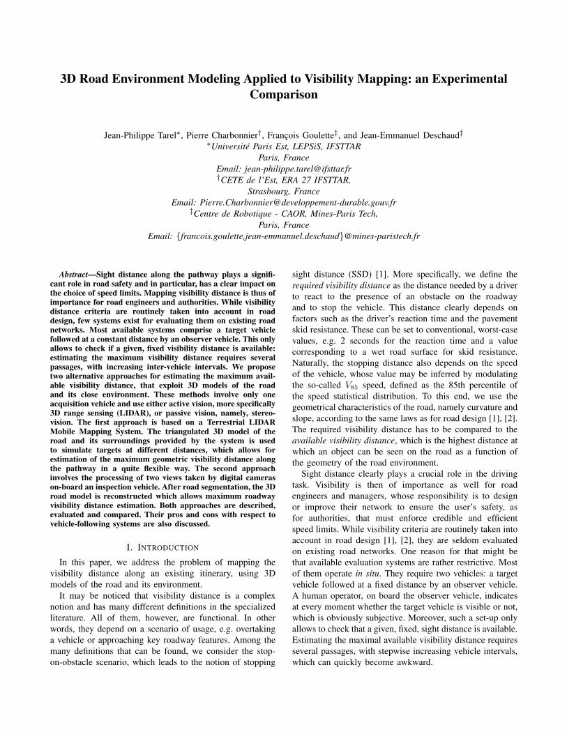
(a) (b)

Figure 1. (a) The experimental vehicle, LARA3D; (b) an example of obtained 3D point cloud.

We believe that using 3D models offer an interesting

alternative to vehicle-following systems, by providing more

flexible, accurate and objective visibility assessment tools. In

this paper, we investigate the use of two kinds of such nu-

merical models for visibility estimation. To our knowledge,

no such system was previously reported in the literature,

excepted from a recent work, based on airborne LIDAR

data [3]. In contrast, we consider terrestrial sensors, based

on either active or passive vision technologies.

More specifically, we first investigate (Sec. II) the use

of 3D data provided by a LIDAR terrestrial Mobile Map-

ping System. As the inspection vehicle moves, 3D points

are sampled along the road and registered in an absolute

reference system thanks to the use of INS and GPS sensors.

The resulting point cloud is processed off-line to construct

a triangulated 3D model of the road and its environment.

Traditional visualization techniques such as ray-tracing or

z-buffering are then used to implement the computation of

available visibility.

Since road visibility evaluation by drivers is essentially

a visual task, the second approach we propose (Sec. III)

exploits images taken by cameras mounted on an inspection

vehicle. Using two cameras allows modeling the 3D shape

of the road, through stereovision. This model is exploited

in conjunction with the results of an original roadway

segmentation technique to evaluate the available visibility

of the road.

Evaluating such systems on existing roads is not an

obvious task due to the difficulty of establishing a reliable

ground-truth. We have chosen to consider an operational

vehicle-following system as a reference. We provide exper-

imental comparisons on both a test-track and a trafficked

road section (Sec. IV).

We close the paper (Sec. V) by a discussion about the pros

and cons of the proposed methods and working perspectives.

II. MOBILE LIDAR-BASED METHOD

In this approach, we build a 3D model of the road envi-

ronment with a mobile mapping system based on LIDAR

sensors. Then, we compute the visibility distance with a

software ray-tracing algorithm directly on 3d mesh. We will

detail in this section all processes (system, modeling and

distance computation) specific to the application of visibility

distance estimation.

A. Active sensor acquisition system

Our mobile mapping system, called LARA3D, is a pro-

totype with the following sensors: positioning sensors (GPS

and IMU), range sensors (two SICK laser scanners) and

photogrammetric sensors (Pike and Canon cameras). The

location of the vehicle is calculated using a Kalman Filter

with GPS/IMU inspired from [4]. The laser scanners are

installed on the roof of the vehicle at about 2.7 m height to

scan a plane perpendicular to the driving direction. Knowing

the geographic location of the vehicle, we register the

successive laser cross sections obtained over the vehicle’s

passage like Fig. 1. This provide coverage of roads and their

surroundings (buildings, vegetation) in the form of a dense

3D point cloud as seen on Fig. 1. The number of points per

kilometer depends on the vehicle’s speed: at 50 km/h, we

have around 2000000 points per kilometer.

B. 3D Road environment modeling

The next step is to build a realistic 3D model of the

environment from this 3D point cloud. Modeling the en-

vironment from raw laser data is done by following a set of

processes. Here is an overview of the processes applied to

our laser data: automatic removal of artifacts in laser cross

sections, decimation of neighborhood points, denoising,

meshing, detection of flat areas and model simplification.

We detail each of these processes in the following sections.

1) Automatic removal of artifacts: When scanning roads,

the vehicle is driving in normal traffic. Others cars or trucks

are scanned within the environment, causing artifacts. If

these artifacts are not removed, they lead to false objects in

the environment and thus to mistakes in the calculation of

visibility distances. We have developed an automatic method

to remove artifacts on the road. To this end, we process

directly each laser cross section containing a cross section of

the road. Indeed, knowing parameters like the height of the

Figure 2. The automatic removal of artefacts in 3D point clouds.

laser and the distances of the vehicle to the roadside on the

right and on the left of the vehicle, the points out of the road

are removed, as illustrated in Fig. 2. One limitation of this

method is to be dependent on the geometrical configuration

of the laser: it works only if there is road data points in the

laser cross section.

2) Decimation of neighborhood points: Raw point clouds

previously obtained are not uniformly distributed over the

surfaces to be reconstructed. This non-uniform distribution

of points does not allow proper calculation of the normals,

when correct normals are required to obtain a triangulation

without elongated triangle. To avoid this, we perform a

decimation of points per neighborhood: if two points are

closer than some distance d, we remove one of the two

points. This distance d will depend on the resolution of data

in the laser cross section (which depends on the angular

resolution of laser and on the distance of the point to the

laser) and on the resolution of data along the trajectory

(which depends on vehicle speed and on the frequency of

the scanner). Best sampling is achieve when it is uniform in

these two directions.

3) Denoising and Meshing: Once the point cloud is

decimated, we can build the 3D mesh model which is

subject to the presence of noise in the point cloud. It is

therefore necessary to go through a denoising step, prior

to the triangulation. For data denoising, we used the image

processing method called “Non Local Denoising” [5]. This

denoising method works directly on a point cloud and does

not require meshing. The Fig. 3 shows the 3D models with

and without the denoising step, with meshing in order to

facilitate the visualization. After denoising, the mesh is build

Figure 3. The meshing without and with denoising step.

using a triangulation method which is a variant of the Ball

Pivoting Algorithm (BPA) [6].

4) Detecting flat areas and simplification of the model:

After meshing, the obtained 3D models contain around

two millions of triangles per kilometer. As the ray-tracing

algorithm for visibility distance estimation is very slow and

its speed depends on the number of triangles, we need to

simplify the model. We used the fast algorithm for detecting

flat areas in large point clouds described in [7] and then

apply a classical simplification method based on [8] in non-

flat area. These two kind of simplifications leads to arround

200000 triangles per kilometer.

5) The modeling pipeline: We described the different

steps of the processing from the point cloud to the simplified

and sufficiently realistic 3D model of the road environ-

ment. All processes (decimation, denoising, meshing and

simplification) are done off-line but in a time lower that

the acquisition time. As consequence, it would be possible

to directly produce the final triangulated model, without raw

data recording. Fig. 4 shows two examples of obtained 3D

models.

C. Estimating the visibility distance from a 3D model

The definition of the available visibility distance we use

in this approach is purely geometric and does not involve

any photometric or meteorological consideration. It involves

a target and an observer. The target may either be placed

at a fixed distance from the observation point, to assess

the availability of a specific distance, or it may be moved

away from the observation point until it becomes invisible,

to estimate the maximum visibility distance. Conventional

values can be found in the road design literature, see [2],

Figure 4. Two examples of obtained 3D models of the road environmentused for visibility distance estimation.

for both the location of the observer and the geometry

and position of the target. Both the viewpoint and the

target are centered on the road lane axis. Typically, the

viewpoint is located 1 m high, which roughly corresponds

to a mean driver’s eye position. The conventional target is a

pair of points that model a vehicle’s tail lights. For visibility

distance computation, we require a line-of-sight connection

between the tail lights and the driver’s eyes. Ray-tracing

algorithms are well-suited for this task. We also found it

realistic to consider a parallelepiped (1.5 × 4 × 1.3 m) to

model a vehicle. We found that a good rule of thumb was

to consider the target as visible if 5% of its surface is visible.

The threshold was set experimentally, in such a way that the

results of the test would be comparable to the ones obtained

when using the conventional target.

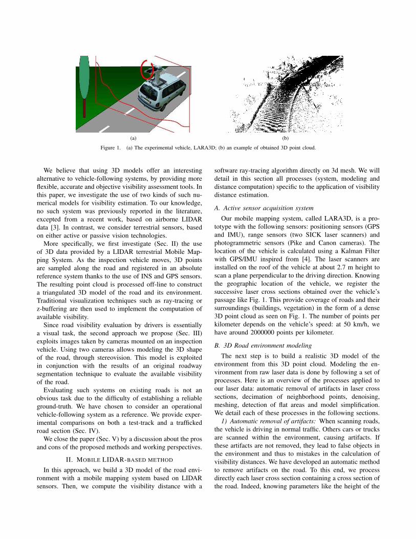
We developed a specific software application (see Fig. 5),

that allows to walk through the 3D model (which can be

visualized as a point cloud or a surface mesh). The trajectory

of the inspection vehicle on the road may also be visualized

in the 3D model. Volumetric or point-wise targets may

be placed at different distances from the viewpoint (see

Fig. 6). To make the interpretation easier, images of the road

scene may be visualized along the 3D model. All views are

synchronized and the interface is completely reconfigurable.

The software implements both required and available visi-

bility distance computation. For the point-wise, conventional

target, we use a software ray-tracing algorithm. When the

volumetric target is used, we exploit the Graphical Process-

ing Unit’s capabilities. More specifically, the target is first

drawn in the graphical memory, then the scene is rendered

using Z-buffering and finally, an occlusion-query request

Figure 6. Example of 3D model (gray triangles) with targets (in green).Top: pairs of points representing tail lights; Bottom: volumetric target.

(which is standard in up-to-date OpenGL implementations)

provides the percentage of visible target surface. The target

is zoomed on and centered in the scene, to mimic the focus-

of-attention mechanism of a human observer.

The visibility distance can be computed at every point

of the trajectory (i.e. every 1 meter) or with a fixed step

(typically, 5 or 10 meters) to speed up computations. Two

different ways of computing the visibility are implemented.

In the first case, a fixed distance is maintained between the

observation point and the target (as for vehicle-following

systems). The output is a binary function which indicates at

every position whether the prescribed distance is available or

not. In the second case, for every position of the observation

point, the target is moved away as long as it is visible and

the maximum available visibility distance is recorded.

III. MOBILE STEREOVISION METHOD

The available visibility distance can be defined as the

maximum distance of points belonging to the image of

the road. This distance can be estimated with stereovision

looking at the road ahead the vehicle. This distance is similar

to the one perceived by the driver, when the distance between

the driver’s eye and the cameras is small.

A. Passive sensor acquisition system

A experimental inspection vehicle was developed for

stereo pair of images acquisition. The images are acquired

every 5 meters, independently of the vehicle speed. Pre-

liminary to every acquisition, the stereo head is calibrated

intrinsically and extrinsically with respect to the road using a

grid painted on the road. The acquired images are rectified

Figure 5. Interface of the sight distance computation software. The top-left panel displays the original point cloud. The top-right panel shows thetriangulated model (in grey), the trajectory of the LIDAR system (in blue) and a parallelepiped target placed 100 m ahead of the observation point (ingreen). At the bottom right, an image of the scene is displayed. Finally, the bottom-left panel displays the required visibility (black) and the estimatedavailable visibility (magenta) vs. the curvilinear abscissa. The vertical line shows the current position. The curves show that the available visibility is notsufficient in this situation.

(a) (b) (c)

Figure 7. (a) Experimental inspection vehicle with two digital cameras for stereovision; (b),(c): stereo pair of images acquired by the vehicle.

and corrected of the geometrical distortions of the lenses.

Lens vignetting is also corrected.

B. Local road modeling

On each of the rectified stereo pair, a two-step processing

is performed to obtain the local road model: segmentation

of the roadway on left and right images using color informa-

tion, 3D reconstruction of the edges in the road regions of the

left and right images allowing to estimate a 3D parametric

model of the road surface.

The first step of the processing consists in classifying

each pixel, in left and right images, as road or non-road.

Following the segmentation approach proposed in [9], this

segmentation consists on an iterative learning of the col-

orimetric characteristics of both the road and the non-road

pixels, along the image sequence. To this end, pixels in

the bottom center of each image are assumed to belong

to the road class, while pixels in the top left and right

regions are assumed non-road elements. These regions may

be visualized in the left image of Fig. 8. The algorithm being

run in batch, the road and non-road color characteristics are

collected in following images. The advantage is that it allows

sampling road colors at different distances ahead of the

current image. This strategy leads to improved segmentation

results in the presence of lighting perturbations, shadows,

variations of pavement color. Once the road and non-road

color models are built, the image is segmented in two classes

by a region growing algorithm, starting from the road (i.e.

bottom center) part of the image. Fig. 8, center image, shows

an example of segmentation result. To keep a correct road

color model, occlusions of the road region can be filtered

out by removing colors which are not usually found on the

pavement.

The second step consists in extracting the edges in the

left and right road regions segmented in the first step

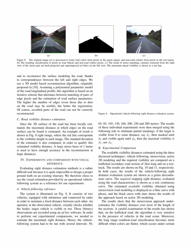
(a) (b) (c)

Figure 8. The original image (a) is processed to learn road colors from pixels in the green region, and non-road colours from pixels in the red region.(b) The resulting classification of pixels as road (black) and non-road (white) pixels. (c) The result of stereo matching: contours extracted from the rightview of the stereo pair are back-projected and superimposed (in blue) on the left view. The maximum ahead visibility is shown as a red line.

and to reconstruct the surface modeling the road, thanks

to correspondences between the left and right edges. We

use a 3D model based reconstruction algorithm, originally

proposed in [10]. Assuming a polynomial parametric model

of the road longitudinal profile, this algorithm is based on an

iterative scheme that alternates between matching of pairs of

edge pixels and the estimation of road surface parameters.

The higher the number of edges (even those due to dust

on the road may be useful), the better the registration.

Of course, occulted parts of the road can not be correctly

reconstructed.

C. Road visibility distance estimation

Once the 3D surface of the road has been locally esti-

mated, the maximum distance at which edges on the road

surface can be found is estimated. An example of result is

shown in Fig. 8 right image, where the red line corresponds

to the visibility height in each image. The standard deviation

of the estimator is also computed, in order to qualify this

estimated visibility distance. A large stereo basis of 1 meter

is used to have enough accuracy in the reconstruction at

large distances.

IV. EXPERIMENTS AND COMPARISON WITH VISUAL

REFERENCE

Evaluating sight distance estimation methods is a rather

difficult task because it is quite impossible to design a proper

ground truth on an existing itinerary. We therefore chose to

use the visual estimation provided by an operational vehicle-

following system as a reference for our experiments.

A. Vehicle-following reference

The system is illustrated on Fig. 9. It consists of two

vehicles, equipped with odometers and connected by radio

in order to maintain a fixed distance between each other. An

operator, in the observation vehicle, visually checks whether

the leader, target vehicle is visible or not. These (binary)

observations are recorded using an ad hoc software. In order

to perform our experimental comparisons, we needed to

estimate the maximum sight distance. Hence, the vehicle-

following system had to be run with several intervals: 50,

Observation vehicle Target vehicle

Radio

GPS Odometer

Modem Radio

OdometerModem

Predifinedinter-distance

Figure 9. Operational vehicle-following sight distance evaluation system.

65, 85, 105, 130, 160, 200, 250 and 280 meters. The results

of these individual experiments were then merged using the

following rule to eliminate partial maskings: if the target is

visible from 0 to some distance, say d1, then masked until

d2 and visible again until d3, then the maximal visibility is

d1, not d3.

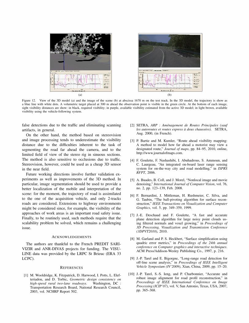
B. Experimental Comparison

The available visibility distances estimated using the three

discussed techniques: vehicle following, stereovision, active

3D modeling and the required visibility are compared on a

trafficked secondary road section of 2km long and on a test-

track. The results are shown on Fig. 10 and 11, respectively.

In both cases, the results of the vehicle-following sight

distance evaluation system are shown as a green discontin-

uous curve. The required stopping sight distance, evaluated

using the road characteristics is shown as a red, continuous

curve. The estimated available visibility obtained using

stereovision road modeling is displayed as a blue curve with

pluses, and the black curve with stars shows the results of

the approach based on active 3D modeling.

The results show that the stereovision approach under-

estimates the visibility distance over most of the length of

the sections. A careful examination of the results has shown

that, on the trafficked road, the algorithm is very sensitive

to the presence of vehicles in the road scene. Moreover,

the long range road/non-road classification becomes more

difficult when colors are flatter, which occurs under certain

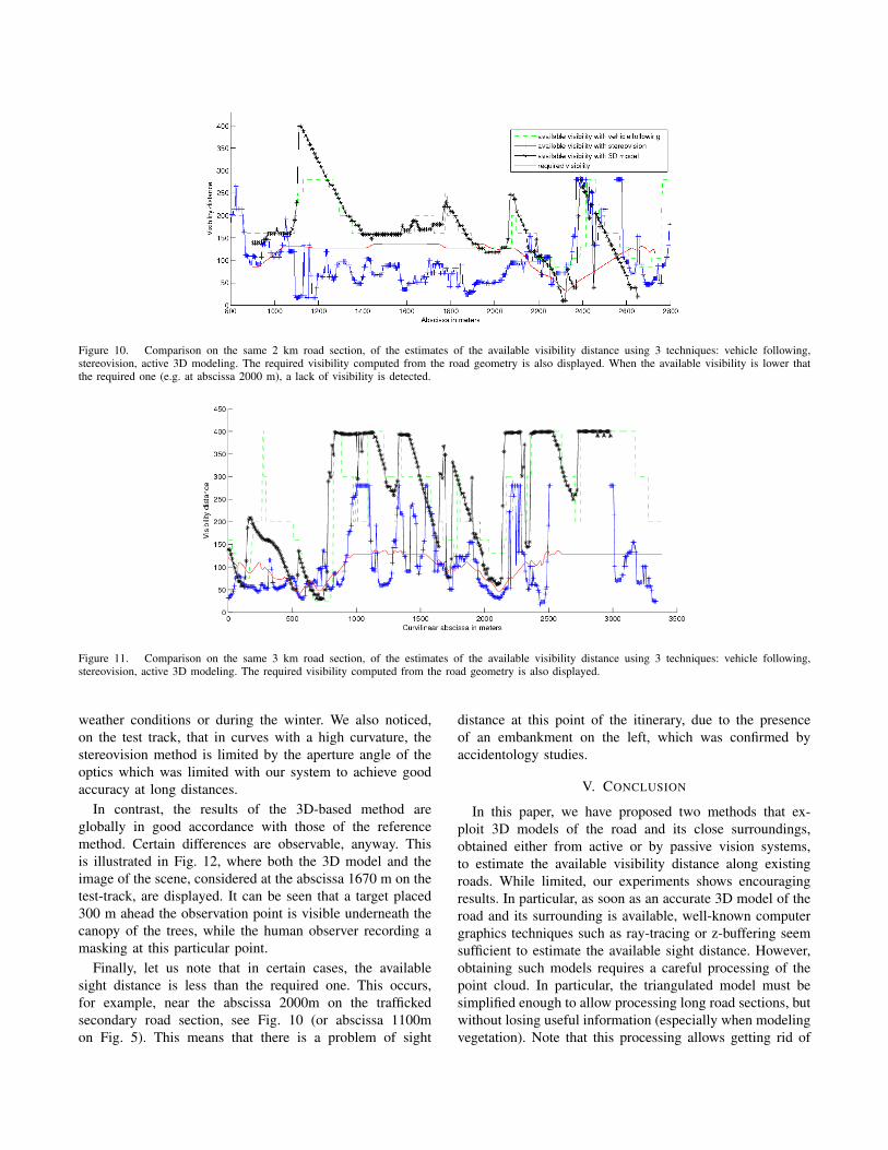
Figure 10. Comparison on the same 2 km road section, of the estimates of the available visibility distance using 3 techniques: vehicle following,stereovision, active 3D modeling. The required visibility computed from the road geometry is also displayed. When the available visibility is lower thatthe required one (e.g. at abscissa 2000 m), a lack of visibility is detected.

Figure 11. Comparison on the same 3 km road section, of the estimates of the available visibility distance using 3 techniques: vehicle following,stereovision, active 3D modeling. The required visibility computed from the road geometry is also displayed.

weather conditions or during the winter. We also noticed,

on the test track, that in curves with a high curvature, the

stereovision method is limited by the aperture angle of the

optics which was limited with our system to achieve good

accuracy at long distances.

In contrast, the results of the 3D-based method are

globally in good accordance with those of the reference

method. Certain differences are observable, anyway. This

is illustrated in Fig. 12, where both the 3D model and the

image of the scene, considered at the abscissa 1670 m on the

test-track, are displayed. It can be seen that a target placed

300 m ahead the observation point is visible underneath the

canopy of the trees, while the human observer recording a

masking at this particular point.

Finally, let us note that in certain cases, the available

sight distance is less than the required one. This occurs,

for example, near the abscissa 2000m on the trafficked

secondary road section, see Fig. 10 (or abscissa 1100m

on Fig. 5). This means that there is a problem of sight

distance at this point of the itinerary, due to the presence

of an embankment on the left, which was confirmed by

accidentology studies.

V. CONCLUSION

In this paper, we have proposed two methods that ex-

ploit 3D models of the road and its close surroundings,

obtained either from active or by passive vision systems,

to estimate the available visibility distance along existing

roads. While limited, our experiments shows encouraging

results. In particular, as soon as an accurate 3D model of the

road and its surrounding is available, well-known computer

graphics techniques such as ray-tracing or z-buffering seem

sufficient to estimate the available sight distance. However,

obtaining such models requires a careful processing of the

point cloud. In particular, the triangulated model must be

simplified enough to allow processing long road sections, but

without losing useful information (especially when modeling

vegetation). Note that this processing allows getting rid of

(a) (b)

Figure 12. View of the 3D model (a) and the image of the scene (b) at abscissa 1670 m on the test track. In the 3D model, the trajectory is show asa blue line with white dots. A volumetric target placed at 300 m ahead the observation point is visible in the green circle. At the bottom of each image,sight visibility distances are show: in black, required visibility; in purple, available visibility estimated from the active 3D model; in light brown, availablevisibility using the vehicle-following system.

false detections due to the traffic and eliminating scanning

artifacts, in general.

On the other hand, the method based on stereovision

and image processing tends to underestimate the visibility

distance due to the difficulties inherent to the task of

segmenting the road far ahead the camera, and to the

limited field of view of the stereo rig in sinuous sections.

The method is also sensitive to occlusions due to traffic.

Stereovision, however, could be used as a cheap 3D sensor

in the near field.

Future working directions involve further validation ex-

periments as well as improvements of the 3D method. In

particular, image segmentation should be used to provide a

better localization of the mobile and interpretation of the

scene: for the moment, the trajectory of road is assimilated

to the one of the acquisition vehicle, and only 2-tracks

roads are considered. Extensions to highway environments

might be considered since, for example, the visibility of the

approaches of work areas is an important road safety issue.

Finally, to be routinely used, such methods require that the

scalability problem be solved, which remains a challenging

issue.

ACKNOWLEDGEMENTS

The authors are thankful to the French PREDIT SARI-

VIZIR and ANR-DIVAS projects for funding. The VISU-

LINE data was provided by the LRPC St Brieuc (ERA 33

LCPC).

REFERENCES

[1] M. Wooldridge, K. Fitzpatrick, D. Harwood, I. Potts, L. Elef-teriadou, and D. Torbic, Geometric design consistency onhigh-speed rural two-lane roadways. Washington, DC :Transportation Research Board, National Research Council,2003, vol. NCHRP Report 502.

[2] SETRA, ARP : Amenagement de Routes Principales (saufles autoroutes et routes express a deux chaussees). SETRA,Aug. 2000, (in French).

[3] P. Bartie and M. Kumler, “Route ahead visibility mapping:A method to model how far ahead a motorist may view adesignated route,” Journal of maps, pp. 84–95, 2010, online,http://www.journalofmaps.com.

[4] F. Goulette, F. Nashashibi, I. Abuhadrous, S. Ammoun, andC. Laurgeau, “An integrated on-board laser range sensingsystem for on-the-way city and road modelling,” in ISPRSRFPT, 2006.

[5] A. Buades, B. Coll, and J. Morel, “Nonlocal image and moviedenoising,” International Journal of Computer Vision, vol. 76,no. 2, pp. 123–139, Feb. 2008.

[6] F. Bernardini, J. Mittleman, H. Rushmeier, C. Silva, andG. Taubin, “The ball-pivoting algorithm for surface recon-struction,” IEEE Transactions on Visualization and ComputerGraphics, vol. 5, pp. 349–359, 1999.

[7] J.-E. Deschaud and F. Goulette, “A fast and accurateplane detection algorithm for large noisy point clouds us-ing filtered normals and voxel growing,” in Proceedings of3D Processing, Visualization and Transmission Conference(3DPVT2010), 2010.

[8] M. Garland and P. S. Heckbert, “Surface simplification usingquadric error metrics,” in Proceedings of the 24th annualconference on Computer graphics and interactive techniques.ACM Press/Addison-Wesley Publishing Co., 1997, p. 216.

[9] J.-P. Tarel and E. Bigorgne, “Long-range road detection foroff-line scene analysis,” in Proceedings of IEEE IntelligentVehicle Symposium (IV’2009), Xian, China, 2009, pp. 15–20.

[10] J.-P. Tarel, S.-S. Ieng, and P. Charbonnier, “Accurate androbust image alignment for road profil reconstruction,” inProceedings of IEEE International Conference on ImageProcessing (ICIP’07), vol. V, San Antonio, Texas, USA, 2007,pp. 365–368.