Embed Size (px)
Citation preview
3D Reconstruction
and
Camera Calibration
from
2D Images
by
Arne Henrichsen
Submitted to the Department of Electrical Engineeringin fulfilment of the requirements for the degree of
Master of Science in Engineering
at the
UNIVERSITY OF CAPE TOWN
December 2000
© University of Cape Town 2000

Make some space
Declaration
I, Arne Henrichsen, declare that this dissertation is my own work, except where otherwise stated.
It is being submitted for the degree of Master of Science in Engineering at the University of
Cape Town and it has not been submitted before for any degree or examination, at any other
university.
Signature of Author . . . . . . . . . . . . . . . . . . . . . . . . . . . . . . . . . . . . . . . . . . . . . . . . . . . . . . . . . . . . . . . . . .
Cape Town
December 2000
i


Acknowledgements
I would like to thank my supervisor, Professor Gerhard de Jager, for the opportunity he gave me
to work in the Digital Image Processing group and for his enthusiasm and guidance throughout
this project.
I also wish to thank:
• The National Research Foundation and DebTech for their generous financial support.
• All the members of the Digital Image Processing group for providing an interesting and
stimulating working environment, and in particular Fred Nicolls for his help with my
many questions.
• Marthinus C. Briers from the Department of Geomatics at UCT for his help in calibrating
my camera.
• David Liebowitz from the Department of Engineering Science at Oxford for helping me
understand his calibration method.
iii

Abstract
A 3D reconstruction technique from stereo images is presented that needs minimal intervention
from the user.
The reconstruction problem consists of three steps, each of which is equivalent to the estimation
of a specific geometry group. The first step is the estimation of the epipolar geometry that exists
between the stereo image pair, a process involving feature matching in both images. The second
step estimates the affine geometry, a process of finding a special plane in projective space by
means of vanishing points. Camera calibration forms part of the third step in obtaining the
metric geometry, from which it is possible to obtain a 3D model of the scene.
The advantage of this system is that the stereo images do not need to be calibrated in order
to obtain a reconstruction. Results for both the camera calibration and reconstruction are
presented to verify that it is possible to obtain a 3D model directly from features in the images.
v


Contents
Declaration i
Acknowledgements iii
Abstract v
Contents vi
List of Figures xi
List of Tables xv
List of Symbols xix
Nomenclature xxi
1 Introduction 1
1.1 General Overview . . . . . . . . . . . . . . . . . . . . . . . . . . . . . . . . 1
1.2 The 3D reconstruction problem . . . . . . . . . . . . . . . . . . . . . . . . .2
1.3 Outline of the thesis . . . . . . . . . . . . . . . . . . . . . . . . . . . . . . . 4
2 Stratification of 3D Vision 7
2.1 Introduction . . . . . . . . . . . . . . . . . . . . . . . . . . . . . . . . . . . 7
vii
viii CONTENTS
2.2 Projective Geometry . . . . . . . . . . . . . . . . . . . . . . . . . . . . . . 8
2.2.1 Homogeneous Coordinates and other Definitions . . . . . . . . . . .8
2.2.2 The Projective Plane . . . . . . . . . . . . . . . . . . . . . . . . . . 9
2.2.3 The Projective Space . . . . . . . . . . . . . . . . . . . . . . . . . .13
2.2.4 Discussion . . . . . . . . . . . . . . . . . . . . . . . . . . . . . . .16
2.3 Affine Geometry . . . . . . . . . . . . . . . . . . . . . . . . . . . . . . . .16
2.3.1 The Affine Plane . . . . . . . . . . . . . . . . . . . . . . . . . . . .16
2.3.2 The Affine Space . . . . . . . . . . . . . . . . . . . . . . . . . . . .17
2.3.3 Discussion . . . . . . . . . . . . . . . . . . . . . . . . . . . . . . .18
2.4 Metric Geometry . . . . . . . . . . . . . . . . . . . . . . . . . . . . . . . .19
2.4.1 The Metric Plane . . . . . . . . . . . . . . . . . . . . . . . . . . . .19
2.4.2 The Metric Space . . . . . . . . . . . . . . . . . . . . . . . . . . . .20
2.4.3 Discussion . . . . . . . . . . . . . . . . . . . . . . . . . . . . . . .22
2.5 Euclidean Geometry . . . . . . . . . . . . . . . . . . . . . . . . . . . . . .23
2.6 Notations . . . . . . . . . . . . . . . . . . . . . . . . . . . . . . . . . . . .23
3 Camera Model and Epipolar Geometry 25
3.1 Introduction . . . . . . . . . . . . . . . . . . . . . . . . . . . . . . . . . . .25
3.2 Camera Model . . . . . . . . . . . . . . . . . . . . . . . . . . . . . . . . .25
3.2.1 Camera Calibration Matrix . . . . . . . . . . . . . . . . . . . . . . .27
3.2.2 Camera Motion . . . . . . . . . . . . . . . . . . . . . . . . . . . . .28
3.3 Epipolar Geometry . . . . . . . . . . . . . . . . . . . . . . . . . . . . . . .28
4 Fundamental Matrix Estimation 31
4.1 Introduction . . . . . . . . . . . . . . . . . . . . . . . . . . . . . . . . . . .31
4.2 Linear Least-Squares Technique . . . . . . . . . . . . . . . . . . . . . . . .31
CONTENTS ix
4.3 Minimising the Distances to Epipolar Lines . . . . . . . . . . . . . . . . . .33
4.4 Least-Median-of-Squares method . . . . . . . . . . . . . . . . . . . . . . .35
4.5 RANSAC . . . . . . . . . . . . . . . . . . . . . . . . . . . . . . . . . . . . 38
5 Corner Matching 39
5.1 Introduction . . . . . . . . . . . . . . . . . . . . . . . . . . . . . . . . . . .39
5.2 Establishing Matches by Correlation . . . . . . . . . . . . . . . . . . . . . .40
5.3 Support of each Match . . . . . . . . . . . . . . . . . . . . . . . . . . . . .40
5.4 Initial Matches by Singular Value Decomposition . . . . . . . . . . . . . . .43
5.5 Resolving False Matches . . . . . . . . . . . . . . . . . . . . . . . . . . . .45
5.6 Results . . . . . . . . . . . . . . . . . . . . . . . . . . . . . . . . . . . . . .46
6 Camera Calibration 51
6.1 Introduction . . . . . . . . . . . . . . . . . . . . . . . . . . . . . . . . . . .51
6.2 Classical Calibration Methods . . . . . . . . . . . . . . . . . . . . . . . . .52
6.2.1 Introduction . . . . . . . . . . . . . . . . . . . . . . . . . . . . . . .52
6.2.2 Estimating the Perspective Projection Matrix . . . . . . . . . . . . .53
6.2.3 Extracting the Camera Calibration Matrix . . . . . . . . . . . . . . .54
6.2.4 Other Methods . . . . . . . . . . . . . . . . . . . . . . . . . . . . .54
6.3 Selfcalibration using Kruppa’s Equations . . . . . . . . . . . . . . . . . . .55
6.3.1 Introduction . . . . . . . . . . . . . . . . . . . . . . . . . . . . . . .55
6.3.2 Kruppa’s Equations . . . . . . . . . . . . . . . . . . . . . . . . . . .56
6.4 Selfcalibration in Single Views . . . . . . . . . . . . . . . . . . . . . . . . .58
6.4.1 Introduction . . . . . . . . . . . . . . . . . . . . . . . . . . . . . . .58
6.4.2 Some Background . . . . . . . . . . . . . . . . . . . . . . . . . . .58
6.4.3 Calibration Method 1 . . . . . . . . . . . . . . . . . . . . . . . . . .59
x CONTENTS
6.4.4 Calibration Method 2 . . . . . . . . . . . . . . . . . . . . . . . . . .62
6.4.5 Conclusion . . . . . . . . . . . . . . . . . . . . . . . . . . . . . . .65
6.5 Calibration using a Planar Pattern . . . . . . . . . . . . . . . . . . . . . . .66
6.5.1 Introduction . . . . . . . . . . . . . . . . . . . . . . . . . . . . . . .66
6.5.2 Homography between the Planar Object and its Image . . . . . . . .66
6.5.3 Calculating the Camera Calibration Matrix . . . . . . . . . . . . . .69
6.5.4 Results . . . . . . . . . . . . . . . . . . . . . . . . . . . . . . . . .71
7 Stratified 3D Reconstruction 73
7.1 Introduction . . . . . . . . . . . . . . . . . . . . . . . . . . . . . . . . . . .73
7.2 3D Reconstruction . . . . . . . . . . . . . . . . . . . . . . . . . . . . . . .74
7.2.1 Projective Reconstruction . . . . . . . . . . . . . . . . . . . . . . .74
7.2.2 Affine Reconstruction . . . . . . . . . . . . . . . . . . . . . . . . .75
7.2.3 Metric Reconstruction . . . . . . . . . . . . . . . . . . . . . . . . .76
7.2.4 Reconstruction Results . . . . . . . . . . . . . . . . . . . . . . . . .77
7.3 3D Textured Model . . . . . . . . . . . . . . . . . . . . . . . . . . . . . . .78
7.3.1 Rectification of Stereo Images . . . . . . . . . . . . . . . . . . . . .80
7.3.2 Dense Stereo Matching . . . . . . . . . . . . . . . . . . . . . . . . .83
7.3.3 Results . . . . . . . . . . . . . . . . . . . . . . . . . . . . . . . . .86
7.4 Other Reconstruction Results . . . . . . . . . . . . . . . . . . . . . . . . . .86
7.5 Conclusion . . . . . . . . . . . . . . . . . . . . . . . . . . . . . . . . . . .87
8 Conclusions 89
A Feature Extraction 91
A.1 Corner Detection . . . . . . . . . . . . . . . . . . . . . . . . . . . . . . . .91
CONTENTS xi
A.1.1 Kitchen and Rosenfeld Corner Detector . . . . . . . . . . . . . . . .91
A.1.2 Harris-Plessey Corner Detector . . . . . . . . . . . . . . . . . . . .92
A.1.3 Subpixel Corner Detection . . . . . . . . . . . . . . . . . . . . . . .93
A.2 Extracting Straight Lines . . . . . . . . . . . . . . . . . . . . . . . . . . . .95
A.2.1 Line-support Regions . . . . . . . . . . . . . . . . . . . . . . . . . .95
A.2.2 Interpreting the Line-Support Region as a Straight Line . . . . . . . .96
B Vanishing Point Estimation 99
C The Levenberg-Marquardt Algorithm 101
C.1 Newton Iteration . . . . . . . . . . . . . . . . . . . . . . . . . . . . . . . .101
C.2 Levenberg-Marquardt Iteration . . . . . . . . . . . . . . . . . . . . . . . . .102
D Triangulation 103
D.1 Linear Triangulation . . . . . . . . . . . . . . . . . . . . . . . . . . . . . .103
D.2 Nonlinear Triangulation . . . . . . . . . . . . . . . . . . . . . . . . . . . . .104
Bibliography 105

xii CONTENTS
List of Figures
2.1 Cross-ratio of four lines:{l 1, l 2; l 3, l 4}={x1, x2; x3, x4} . . . . . . . . . . . . 11
2.2 Conjugate pointsv1 andv2 with respect to the conicC . . . . . . . . . . . . 13
2.3 Cross-ratio of four planes:{π1, π2; π3, π4}={l 1, l 2; l 3, l 4} . . . . . . . . . . . 14
2.4 Illustration of the Laguerre formula inP2 . . . . . . . . . . . . . . . . . . . 20
2.5 Illustration of the Laguerre formula inP3 . . . . . . . . . . . . . . . . . . . 21
3.1 Perspective Projection . . . . . . . . . . . . . . . . . . . . . . . . . . . . . .26
3.2 Illustration of pixel skew . . . . . . . . . . . . . . . . . . . . . . . . . . . .27
3.3 Epipolar Geometry . . . . . . . . . . . . . . . . . . . . . . . . . . . . . . .29
4.1 Illustration of bucketing technique . . . . . . . . . . . . . . . . . . . . . . .37
4.2 Interval and bucket mapping . . . . . . . . . . . . . . . . . . . . . . . . . .38
5.1 Non-symmetry problem for match strength . . . . . . . . . . . . . . . . . .42
5.2 Repetitive Pattern . . . . . . . . . . . . . . . . . . . . . . . . . . . . . . . .46
5.3 Uniform background scene with markers (Camera Translation) . . . . . . . .48
5.4 Uniform background scene with markers (Camera Rotation) . . . . . . . . .49
5.5 Uniform background scene with markers (Camera Zooming) . . . . . . . . .50
6.1 Common Calibration Pattern . . . . . . . . . . . . . . . . . . . . . . . . . .52
6.2 Calibration Object . . . . . . . . . . . . . . . . . . . . . . . . . . . . . . . .55
xiii

xiv LIST OF FIGURES
6.3 The Image of the Absolute Conic . . . . . . . . . . . . . . . . . . . . . . . .56
6.4 Image illustrating three orthogonal planes . . . . . . . . . . . . . . . . . . .60
6.5 Three Orthogonal Vanishing Points . . . . . . . . . . . . . . . . . . . . . . .60
6.6 Image illustrating three planes in the scene . . . . . . . . . . . . . . . . . . .63
6.7 Back wall (plane) affine rectified . . . . . . . . . . . . . . . . . . . . . . . .63
6.8 Line Ratio Constraint . . . . . . . . . . . . . . . . . . . . . . . . . . . . . .64
6.9 Constraint Circles . . . . . . . . . . . . . . . . . . . . . . . . . . . . . . . .65
6.10 Planar Calibration Patterns . . . . . . . . . . . . . . . . . . . . . . . . . . .67
6.11 World Coordinate Points of Planar Pattern . . . . . . . . . . . . . . . . . . .68
7.1 Synthetic corner illustrating the vanishing points . . . . . . . . . . . . . . . .76
7.2 Vanishing points defining one line . . . . . . . . . . . . . . . . . . . . . . .77
7.3 Correct estimation of vanishing points . . . . . . . . . . . . . . . . . . . . .78
7.4 Parallel lines estimated in three directions for a stereo image pair . . . . . . .79
7.5 Three convex hulls representing the three planes of the box . . . . . . . . . .80
7.6 Reconstructed convex hulls illustrating the relationship between the three planes
of the box . . . . . . . . . . . . . . . . . . . . . . . . . . . . . . . . . . . . 80
7.7 Rectification Process . . . . . . . . . . . . . . . . . . . . . . . . . . . . . .81
7.8 Rectified stereo image pair with horizontal epipolar lines . . . . . . . . . . .83
7.9 Nine different correlation windows . . . . . . . . . . . . . . . . . . . . . . .84
7.10 Disparity map calculated on stereo image pair . . . . . . . . . . . . . . . . .85
7.11 Reconstructed 3D texture model . . . . . . . . . . . . . . . . . . . . . . . .86
7.12 Simple Reconstruction of a calibration pattern . . . . . . . . . . . . . . . . .87
A.1 Illustration of subpixel corner estimation . . . . . . . . . . . . . . . . . . . .94
A.2 Gradient Space Partioning . . . . . . . . . . . . . . . . . . . . . . . . . . .96

LIST OF FIGURES xv
A.3 Two planes intersecting in a straight line . . . . . . . . . . . . . . . . . . . .97
A.4 Comparison between the Hough Transform and Burns Line Algorithm . . . .98
B.1 Maximum Likelihood Estimate of Vanishing Point . . . . . . . . . . . . . .99

xvi LIST OF FIGURES

List of Tables
6.1 Comparison of the real and estimated internal parameters of the camera . . .71
7.1 Angles between the three reconstructed convex hulls . . . . . . . . . . . . .77
xvii

xviii LIST OF TABLES

List of Symbols
Pn — Projective Space (n-dimensions)
An — Affine Space (n-dimensions)
l — Line in Projective Space
π — Plane in Projective Space
l ∞ — Line at Infinity
π∞ — Plane at Infinity
m — Homogeneous Coordinate Vector of Vectorm
� — Absolute Conic
�∗ — Dual Absolute Conic
ω∞ — Image of the Absolute Conic
ω∗
∞— Image of the Dual Absolute Conic
K — Camera Calibration Matrix
R — Rotation Matrix
t — Translation Vector
F — Fundamental Matrix
xix

Nomenclature
2D —Two-dimensional space, eg: the image plane.
3D —Three-dimensional space.
CCD — Charged Coupled Device.
det(S) — Determinant of the square matrixS.
SVD —Singular Value Decomposition of a Matrix.
LMedS — Least-Median-of-Squares Method.
SSD —Sum of Squared Differences.
MLE — Maximum Likelihood Estimate.
xxi

Make some space
Chapter 1
Introduction
1.1 General Overview
The objective of this thesis is to present an automatic 3D reconstruction technique that uses
only stereo images of a scene.
The topic of obtaining 3D models from images is a fairly new research field in computer vision.
In photogrammetry, on the other hand, this field is well established and has been around since
nearly the same time as the discovery of photography itself [20]. Whereas photogrammetrists
are usually interested in building detailed and accurate 3D models from images, in the field of
computer vision work is being done on automating the reconstruction problem and implement-
ing an intelligent human-like system that is capable of extracting relevant information from
image data.
This thesis presents a basic framework for doing exactly that. Only stereo image pairs are
considered, as much relevant information is available on this topic.
The two images can be acquired by either two cameras at the same time or by one camera at
a different time instant. It would be possible to extend the principle in this thesis to include a
whole image sequence.
1
2 CHAPTER 1. INTRODUCTION
1.2 The 3D reconstruction problem
Structure from uncalibrated images only leads to a projective reconstruction. Faugeras [7]
defines a matrix called the fundamental matrix, which describes the projective structure of
stereo images. Many algorithms for determining the fundamental matrix have since been
developed: a review of most of them can be found in a paper by Zhang [52]. Robust methods
for determining the fundamental matrix are especially important when dealing with real image
data. This image data is usually in the form of corners (high curvature points), as they can be
easily represented and manipulated in projective geometry. There are various corner detection
algorithms. The ones employed in this thesis are by Kitchen and Rosenfeld [23] and Harris and
Stephens [16]. Alternatively, Taylor and Kriegman [46] develope a reconstruction algorithm
using line segments instead of corners.
Image matching forms a fundamental part of epipolar analysis. Corners are estimated in both
images independently, and the matching algorithm needs to pair up the corner points correctly.
Initial matches are obtained by correlation and relaxation techniques. A new approach by Pilu
[36] sets up a correlation-weighted proximity matrix and uses singular value decomposition to
match up the points. A matching algorithm by Zhang et. al. [54] uses a very robust technique
calledLMedS(Least-Median-of-Squares Method), which is able to discard outliers in the list
of initial matches and calculates the optimal fundamental matrix at the same time.
In order to upgrade the projective reconstruction to a metric or Euclidean one, 3D vision is
divided or stratified into four geometry groups, of which projective geometry forms the basis.
The four geometry strata are projective, affine, metric and Euclidean geometry. Stratification
of 3D vision makes it easier to perform a reconstruction. Faugeras [9] gives an extensive
background on how to achieve a reconstruction by upgrading projective to affine geometry and
affine to metric and Euclidean geometry.
Affine geometry is established by finding theplane at infinityin projective space for both
images. The usual method of finding the plane is by determining vanishing points in both
images and then projecting them into space to obtainpoints at infinity. Vanishing points are the
intersections of two or more imaged parallel lines. This process is unfortunately very difficult
to automate, as the user generally has to select the parallel lines in the images. Some automatic
algorithms try to find dominant line orientations in histograms [28]. Pollefeys [37] introduced
themodulus constraint, from which it is possible to obtain an accurate estimation of the plane
at infinity by determining infinite homographies between views. At least three views need to
be present in order for the algorithm to work properly.
1.2. THE 3D RECONSTRUCTION PROBLEM 3
Camera calibration allows for an upgrade to metric geometry. Various techniques exist to
recover the internal parameters of the camera involved in the imaging process. These parameters
incorporate the focal length, the principal point and pixel skew. The classical calibration
technique involves placing a calibration grid in the scene. The 3D coordinates of markers on
the grid are known and the relationship between these and the corresponding image coordinates
of the same markers allow for the camera to be calibrated. The calibration grid can be replaced
by a virtual object lying in the plane at infinity, called theabsolute conic. Various methods
exist to calculate the absolute conic, andKruppa’s equations[19, 30, 49] form the basis of the
most famous one. These equations provide constraints on the absolute conic and can be solved
by knowing the fundamental matrix between at least three views. Vanishing points can also be
used to calibrate a camera, as a paper by Caprile and Torre [5] shows. This idea is also used in
a method by Liebowitz et. al. [27, 28, 29], which makes use of only a single view to obtain the
camera calibration parameters. A new calibration technique which places a planar pattern of
known dimensions in the scene, but for which 3D coordinates of markers are not known, has
been developed by Zhang [51, 53]. The homography between the plane in the scene and the
image plane is calculated, from which a calibration is possible.
Euclidean geometry is simply metric geometry, but incorporates the correct scale of the scene.
The scale can be fixed by knowing the dimensions of a certain object in the scene.
Up to this point it is possible to obtain the 3D geometry of the scene, but as only a restricted
number of features are extracted, it is not possible to obtain a very complete textured 3D model.
Dense stereo matching techniques can be employed once the the camera projection matrices
for both images are known. Most dense stereo algorithms operate on rectified stereo image
pairs in order to reduce the search space to one dimension. Pollefeys, Koch and van Gool
[39] reparameterise the images with polar coordinates, but need to employ oriented projective
geometry [26] to orient the epipolar lines. Another rectification algorithm by Roy, Meunier and
Cox [42] rectifies on a cylinder instead of a plane. This method is very difficult to implement
as all operations are performed in 3D space. A very simple method implemented in this thesis
is by Fusiello, Trucco and Verri [13, 14], which rectifies the two images by rotating the camera
projection matrices around their optical centres until the focal planes become coplanar.
Two dense stereo matching algorithms have been considered. Koch [24, 25] obtains a 3D
model by extracting depth from rectified stereoscopic images by means of fitting a surface to
a disparity map and performing surface segmentation. A method by Fusiello, Roberto and
Trucco [12] makes use of multiple correlation windows to obtain a good approximation to the
disparity, from which it is possible by means of triangulation to obtain a 3D textured model.
4 CHAPTER 1. INTRODUCTION
1.3 Outline of the thesis
Chapter 2 summarises aspects of projective geometry and also deals with stratification of
3D vision. This chapter is extremely important as it gives a theoretical framework to the
reconstruction problem.
The camera model is introduced in chapter 3, with the emphasis on epipolar geometry. Epipolar
geometry defines the relationship between a stereo image pair. This relationship is in the form
of a matrix, called the fundamental matrix. The fundamental matrix allows for a projective
reconstruction, from which it is then possible to obtain a full Euclidean 3D reconstruction.
Three techniques for the estimation of the fundamental matrix are outlined in chapter 4. One
of the techniques, the Least-Median-of-Squares (LMedS) method, plays a role in the point
matching algorithm, as this method is able to detect false matches and at the same time calculates
a robust estimate of the fundamental matrix. A linear least-squares technique is used as an initial
estimate to the LmedS method.
In chapter 5, a robust matching algorithm is outlined that incorporates two different matching
techniques. The matching process makes use of correlation and relaxation techniques to find
a set of initial matches. With the help of the LMedS method, which makes use of the epipolar
geometry that exists between the two images, the set of initial matches are refined and false
matches are discarded. Some of the limitations of the matching algorithm are described at the
end of the chapter.
Chapter 6 describes four different camera calibration methods with their advantages and disad-
vantages. Some original calibration methods are described that make use of calibration patterns
inside the view of the camera. Selfcalibration is a technique that substitutes the calibration pat-
tern with a virtual object. This object provides constraints to calculate the camera calibration
matrix. It is also possible to obtain the internal parameters of the camera from only a single
view. In order to achieve that, certain measurements in the scene need to be known. The
last calibration method makes use of a planar calibration grid, which is imaged from different
views. The correspondence between the image planes and the planar pattern is used to establish
the calibration matrix.
The complete reconstruction process is presented in chapter 7. Projective, affine and metric
reconstruction processes are described. The estimation of the plane at infinity is described in
detail, and certain criteria are outlined that have to be met in order to obtain an accurate estimate
of the plane. This chapter also describes dense stereo matching in order to obtain a 3D textured

1.3. OUTLINE OF THE THESIS 5
model of the scene. The reconstruction results are also presented in this chapter. Part of a box
is reconstructed, verifying that the reconstruction algorithm functions properly.
Conclusions are drawn in chapter 8.
The appendix summarises various algorithms which are used throughout the thesis:
• Two corner detection algorithms are described together with an algorithm which refines
the corners to subpixel accuracy.
• A straight line finder is outlined which is used to find parallel lines in the images.
• A maximum likelihood estimateis presented which finds the best estimate of a vanishing
point.
• TheLevenberg-Marquardtalgorithm is explained as it is used in all the nonlinear min-
imisation routines.
• Two methods of triangulation are presented which are used in the reconstruction problem.
For a stereo image pair, the individual steps of the reconstruction algorithm are as follows:
1. Corners are detected in each image independently.
2. A set of initial corner matches is calculated.
3. The fundamental matrix is calculated using the set of initial matches.
4. False matches are discarded and the fundamental matrix is refined.
5. Projective camera matrices are established from the fundamental matrix.
6. Vanishing points on three different planes and in three different directions are calculated
from parallel lines in the images.
7. The plane at infinity is calculated from the vanishing points in both images.
8. The projective camera matrices are upgraded to affine camera matrices using the plane
at infinity.
9. The camera calibration matrix (established separately to the reconstruction process) is
used to upgrade the affine camera matrices to metric camera matrices.

6 CHAPTER 1. INTRODUCTION
10. Triangulation methods are used to obtain a full 3D reconstruction with the help of the
metric camera matrices.
11. If needed, dense stereo matching techniques are employed to obtain a 3D texture map of
the model to be reconstructed.
Stereo image pairs were obtained by aWatecr Camera, Model: WAT-202B(PAL) and grabbed
by a Asusr AGP-V3800 Ultra framegrabber. If the scene or model did not contain enough
features needed for the reconstruction, markers were put up at strategic places around the scene.
These markers were usually made up from pieces of paper with straight, parallel lines printed
on them for vanishing point estimation, or stars for the corner and matching algorithms.
Chapter 2
Stratification of 3D Vision
2.1 Introduction
Euclidean geometry describes a 3D world very well. As an example, the sides of objects have
known or calculable lengths, intersecting lines determine angles between them, and lines that
are parallel on a plane will never meet. But when it comes to describing the imaging process
of a camera, the Euclidean geometry is not sufficient, as it is not possible to determine lengths
and angles anymore, and parallel lines may intersect.
3D vision can be divided into four geometry groups or strata, of which Euclidean geometry is
one. The simplest group is projective geometry, which forms the basis of all other groups. The
other groups include affine geometry, metric geometry and then Euclidean geometry. These
geometries are subgroups of each other, metric being a subgroup of affine geometry, and both
these being subgroups of projective geometry.
Each geometry has a group of transformations associated with it, which leaves certain properties
of each geometry invariant. These invariants, when recovered for a certain geometry, allow for
an upgrade to the next higher-level geometry. Each of these geometries will be explained in
terms of their invariants and transformations in the next few sections of this chapter.
Projective geometry allows for perspective projections, and as such models the imaging process
very well. Having a model of this perspective projection, it is possible to upgrade the projective
geometry later to Euclidean, via the affine and metric geometries.
Algebraic and projective geometry forms the basis of most computer vision tasks, especially
in the fields of3D reconstruction from imagesandcamera selfcalibration. Section 2.2 gives
7
8 CHAPTER 2. STRATIFICATION OF 3D VISION
an overview of projective geometry and introduces some of the notation used throughout the
text. Concepts such as points, lines, planes, conics and quadrics are described in two and three
dimensions. The sections that follow describe the same structures, but in terms of affine, metric
and Euclidean geometry.
A standard text covering all aspects of projective and algebraic geometry is by Semple and
Kneebone [44]. Faugeras applies principles of projective geometry to 3D vision and recon-
struction in his book [8]. Other good introductions to projective geometry are by Mohr and
Triggs [33] and by Birchfield [3]. Stratification is described by Faugeras [9] and by Pollefeys
[37].
The following sections are based entirely on the introductions to projective geometry and
stratification by Faugeras [8, 9] and Pollefeys [37].
2.2 Projective Geometry
2.2.1 Homogeneous Coordinates and other Definitions
A point in projective space (n-dimensions),Pn, is represented by a(n + 1)-vector of coordi-
natesx = [x1, . . . , xn+1]T . At least one of thexi coordinates must be nonzero. Two points
represented by(n + 1)-vectorsx and y are considered equal if a nonzero scalarλ exists such
thatx = λy. Equality between points is indicated byx ∼ y. Because scaling is not important
in projective geometry, the vectors described above are calledhomogeneous coordinatesof a
point.
Homogeneous points withxn+1 = 0 are calledpoints at infinityand are related to the affine
geometry described in section 2.3.
A collineation or linear transformation ofPn is defined as a mapping between projective
spaces which preserves collinearity of any set of points. This mapping is represented by a
(m+ 1) × (n + 1) matrix H , for a mapping fromPn7→ Pm. Again for a nonzero scalarλ, H
andλH represent the same collineation. IfH is a(n + 1) × (n + 1) matrix, thenH defines a
collineation fromPn into itself.
A projective basisforPn is defined as any set of(n+2) points ofPn, such that no(n+1) of them
are linearly dependent. The setei = [0, . . . , 1, . . . , 0]T , for i = 1, . . . , n+1, where 1 is in the
i th position, anden+2 = [1, 1, . . . , 1]T form thestandard projective basis. A projective point
of Pn represented by any of its coordinate vectorsx can be described as a linear combination
2.2. PROJECTIVE GEOMETRY 9
of anyn + 1 points of the standard basis:
x =
n+1∑i =1
xi ei . (2.1)
Any projective basis can be transformed by a collineation into a standard projective basis: "let
x1, . . . , xn+2 be n + 2 coordinate vectors of points inPn, no n + 1 of which are linearly
dependent, i.e., a projective basis. Ife1, . . . , en+1, en+2 is the standard projective basis, then
there exists a nonsingular matrixA such thatAei = λi x i , i = 1, . . . , n+2, where theλi are
nonzero scalars; any two matrices with this property differ at most by a scalar factor" [8, 9].
A collineation can also map a projective basis onto a second projective basis: "if x1, . . . , xn+2
and y1, . . . , yn+2 are two sets ofn + 2 coordinate vectors such that in either set non + 1
vectors are linearly dependent, i.e., form two projective basis, then there exists a nonsingular
(n + 1) × (n + 1) matrix P such thatPxi = ρi yi , i = 1, . . . , n + 2, where theρi are scalars,
and the matrixP is uniquely determined apart from a scalar factor" [8, 9].
The proof for both above statements can be found in [8].
2.2.2 The Projective Plane
The projective spaceP2 is known as the projective plane. A point inP2 is defined as a 3-vector
x = [x1, x2, x3]T , with (u, v) = (x1/x3, x2/x3) the Euclidean position on the plane. A line is
also defined as a 3-vectorl = [l1, l2, l3]T and having the equation of
3∑i =1
l i xi = 0. (2.2)
Then a pointx is located on the line if
l T x = 0. (2.3)
This equation can be called theline equation, which means that a pointx is represented by a
set of lines through it, or this equation is called thepoint equation, which means that a linel is
represented by a set of points. These two statements show that there is no difference between
points and lines inP2. This is called theprinciple of duality. Any theorem or statement that
is true for the projective plane can be reworded by substituting points for lines and lines for
points, and the resulting statement will also be true.
10 CHAPTER 2. STRATIFICATION OF 3D VISION
The equation of the line through two pointsx and y is
l = x × y, (2.4)
which is also sometimes calculated as follows:
l = [x]× y, (2.5)
with
[x]× =
0 x3 −x2
−x3 0 x1
x2 −x1 0
(2.6)
being the antisymmetric matrix of coordinate vectorx associated with the cross product. The
intersection point of two lines is also defined by the cross product:x = l 1 × l 2.
All the lines passing through a specific point form thepencil of lines. If two lines l 1 andl 2 are
elements of this pencil, then all the other lines can be obtained as follows:
l = λ1l 1 + λ2l 2, (2.7)
whereλ1 andλ2 are scalars.
Cross-Ratio
If four pointsx1, x2, x3 andx4 are collinear, then they can be expressed by
x i = y + λi z
for two points y and z, and no pointx i coincides withz. Then thecross-ratiois defined as
follows:
{x1, x2; x3, x4} =λ1 − λ3
λ1 − λ4:λ2 − λ3
λ2 − λ4. (2.8)
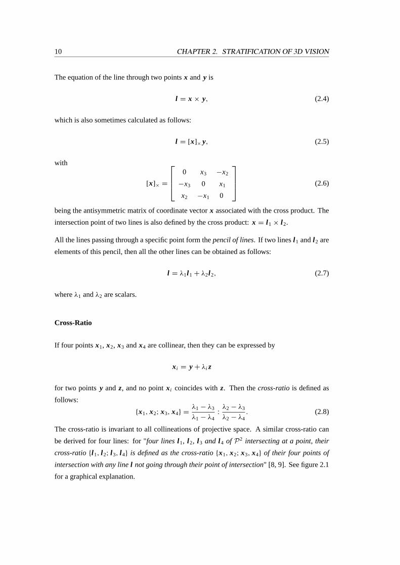
The cross-ratio is invariant to all collineations of projective space. A similar cross-ratio can
be derived for four lines: for "four lines l 1, l 2, l 3 and l 4 of P2 intersecting at a point, their
cross-ratio{l 1, l 2; l 3, l 4} is defined as the cross-ratio{x1, x2; x3, x4} of their four points of
intersection with any linel not going through their point of intersection" [8, 9]. See figure 2.1
for a graphical explanation.
2.2. PROJECTIVE GEOMETRY 11
Figure 2.1: Cross-ratio of four lines:{l 1, l 2; l 3, l 4}={x1, x2; x3, x4}. Figureobtained from [8].
Collineations
A collineation ofP2 is defined by 3× 3 invertible matrices, defined up to a scale factor.
Collineations transform points, lines and pencil of lines1 to points, lines and pencil of lines,
and preserve the cross-ratios. InP2 collineations are called homographies and are represented
by a matrixH . A point x is transformed as follows:
x′∼ Hx . (2.9)
The transformation of a linel is found by transforming the pointsx on the line and then finding
the line defined by these points:
l ′T x′= l T H −1Hx = l T x = 0.
The transformation of the line is then as follows, withH −T= (H −1)T
= (H T )−1:
l ′∼ H −T l . (2.10)
Conics
In Euclidean geometry, second-order curves such as ellipses, parabolas and hyperbolas are
easily defined. In projective geometry, these curves are collectively known asconics. A conic1Thepencil of linesis the set of lines inP2 passing through a fixed point.
12 CHAPTER 2. STRATIFICATION OF 3D VISION
C is defined as the locus of points of the projective plane that satisfies the following equation:
S(x) = xT Cx = 0
or
S(x) =
3∑i, j =1
ci j xi x j = 0,
(2.11)
whereci j = c j i which form C, a 3× 3 symmetric matrix defined up to a scale factor. This
means that the conic depends on 5 parameters. A conic can be visualised by thinking in terms
of Euclidean geometry: a circle is defined as a locus of points with constant distance from the
centre, and a conic is defined as a locus of points with constant cross-ratio to four fixed points,
no three of which are linearly dependent [3].
The principle of duality exists also for conics: thedual conicC∗ or conic envelopeis defined
as the locus of all lines satisfying the following equation:
l T C∗l = 0, (2.12)
whereC∗ is a 3× 3 symmetric matrix defined up to a scale factor and depends also on 5
parameters.
Faugeras [8, 9] shows that the tangentl at a pointx on a conic is defined by
l = CT x = Cx. (2.13)
Then the relationship between the conic and the dual conic is as follows: whenx varies along
the conic, the equationxT Cx = 0 is satisfied and thus the tangent linel to the conic atx
satisfiesl T C−T l = 0. Comparing this to equation (2.12), it shows that the tangents to a conic
defined byC belong to a dual conic defined byC∗∼ C−T .
Transformations of the conic and dual conic with homographyH are as follows (using equations
(2.9) and (2.10)):
x′T C′x′∼ xT H T H −T C H−1Hx = 0
l ′T C∗′
l ′∼ l T H −1HC∗ H T H −T l = 0
2.2. PROJECTIVE GEOMETRY 13
and therefore
C′∼ H −T C H−1 (2.14)
C∗′
∼ HC∗ H T . (2.15)
Poles and Polars
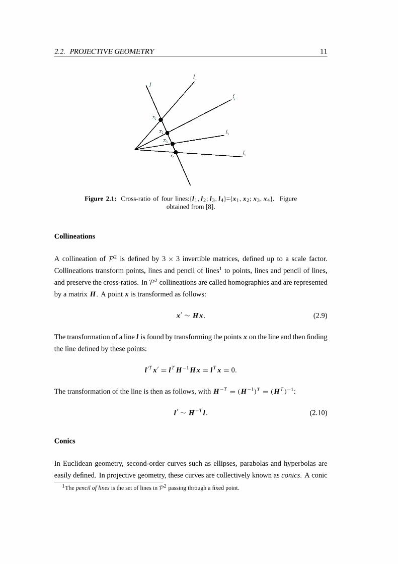
Polesandpolarsare defined as follows: "a pointx and conicC define a linel = Cx. The line
l is called thepolarof x with respect toC, and the pointx is thepoleof l with respect toC. The
polar line l = Cx of the pointx with respect to a conicC intersects the conic in two points at
which tangent lines toC intersect atx. If a pointv1 lies on the polar of another pointv2, then
the two points are said to be conjugate with respect to the conic and satisfyvT1 Cv2 = 0" [29].
Figure 2.2 shows how this is achieved.
Figure 2.2: Pointsv1 andv2, with polarsl 1 and l 2. The pointsv1 andv2 areconjugate with respect to the conicC. Figure obtained from [29].
2.2.3 The Projective Space
The spaceP3 is known as the projective space. A point ofP3 is defined by a 4-vectorx =
[x1, x2, x3, x4]T . The dual entity of the point inP3 is a planeπ , which is also represented by
a 4-vectorπ = [π1, π2, π3, π4]T with equation of
4∑i =1
πi xi = 0. (2.16)
14 CHAPTER 2. STRATIFICATION OF 3D VISION
A point x is located on a plane if the following equation is true:
πT x = 0. (2.17)
The structure which is analogous to the pencil of lines ofP2 is thepencil of planes, the set of
all planes that intersect in a certain line.
Cross-Ratio
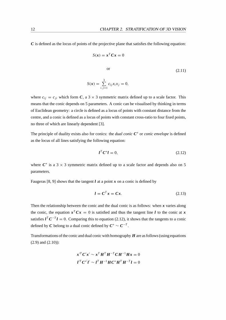
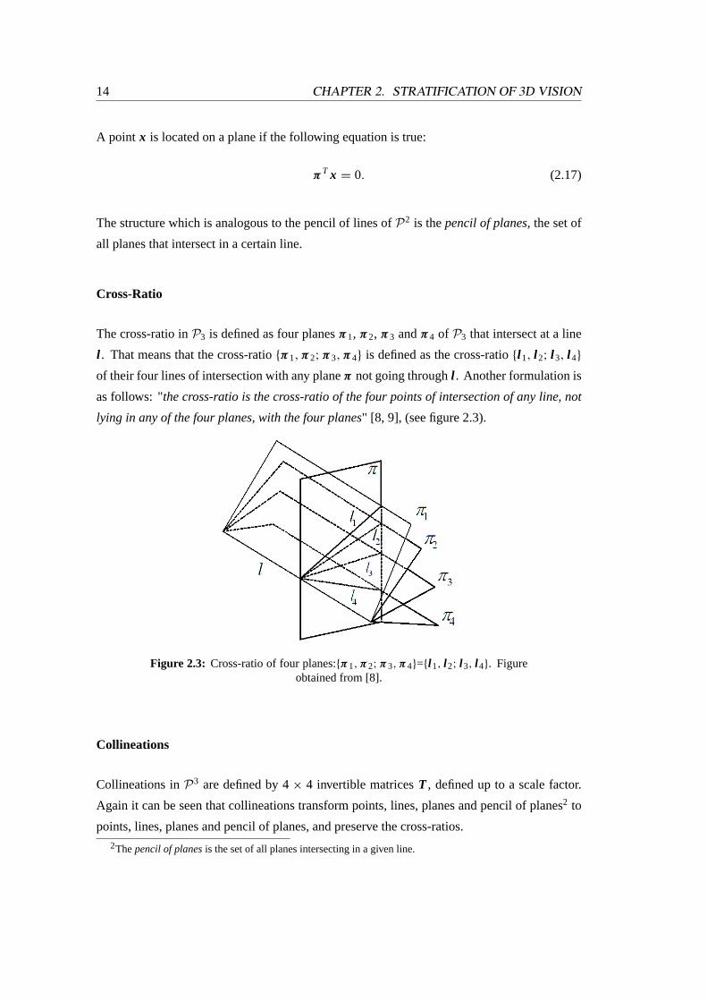
The cross-ratio inP3 is defined as four planesπ1, π2, π3 andπ4 of P3 that intersect at a line
l . That means that the cross-ratio{π1, π2; π3, π4} is defined as the cross-ratio{l 1, l 2; l 3, l 4}
of their four lines of intersection with any planeπ not going throughl . Another formulation is
as follows: "the cross-ratio is the cross-ratio of the four points of intersection of any line, not
lying in any of the four planes, with the four planes" [8, 9], (see figure 2.3).
Figure 2.3: Cross-ratio of four planes:{π1, π2; π3, π4}={l 1, l 2; l 3, l 4}. Figureobtained from [8].
Collineations
Collineations inP3 are defined by 4× 4 invertible matricesT , defined up to a scale factor.
Again it can be seen that collineations transform points, lines, planes and pencil of planes2 to
points, lines, planes and pencil of planes, and preserve the cross-ratios.2Thepencil of planesis the set of all planes intersecting in a given line.
2.2. PROJECTIVE GEOMETRY 15
As was the case inP2, transformationsT of pointsx and planesπ in P3 are as follows:
x′∼ T x (2.18)
and
π ′∼ T−Tπ . (2.19)
Quadrics
The equivalent to a conic inP3 is aquadric. A quadric is the locus of all pointsx satisfying:
S(x) = xT Qx = 0
or
S(x) =
4∑i, j =1
qi j xi x j = 0,
(2.20)
where Q is a 4× 4 symmetric matrix defined up to a scale factor. A quadric depends on 9
independent parameters.
Thedual quadricis the locus of all planesπ satisfying:
πT Q∗π = 0, (2.21)
where Q∗ is a 4× 4 symmetric matrix defined up to a scale factor and also depends on 9
independent parameters.
TransformationsT of the quadric and dual quadric are as follows (similar to transformations
of the conic as in the previous section):
x′T Q′x′∼ xT T T T−T QT−1T x = 0
π ′T Q∗′
π ′∼ πT T−1T Q∗T T T−Tπ = 0
and therefore
Q′∼ T−T QT−1 (2.22)
Q∗′
∼ T Q∗T T . (2.23)
16 CHAPTER 2. STRATIFICATION OF 3D VISION
The quadric can be described as a surface ofP3.
2.2.4 Discussion
Now that a framework for projective geometry has been created, it is possible to define 3D
Euclidean space as embedded in a projective spaceP3. In a similar way, the image plane of
the camera is embedded in a projective spaceP2. Then a collineation exists which maps the
3D space to the image plane,P37→ P2, via a 3× 4 matrix. This will be dealt with in detail in
the next chapter.
As was outlined, the cross-ratio stays invariant to projective transformations or collineations.
The relations ofincidence, collinearityandtangencyare also projectively invariant.
2.3 Affine Geometry
This stratum lies between the projective and metric geometries and contains more structure
than the projective stratum, but less than the metric and Euclidean ones.
2.3.1 The Affine Plane
The line in the projective plane withx3 = 0 is called theline at infinityor l ∞. It is represented
by the vectorl ∞ = [0, 0, 1]T .
The affine plane can be considered to be embedded in the projective plane under a correspon-
dence ofA2→ P2: X = [X1, X2]
T→ [X1, X2, 1]
T . There "is a one-to-one correspondence
between the affine plane and the projective plane minus the line at infinity with equationx3 = 0"
[8, 9]. For a projective pointx = [x1, x2, x3]T that is not on the line at infinity, the affine pa-
rameters can be calculated asX1 =x1x3
andX2 =x2x3
.
To calculate any line’s point at infinity, this line needs to be simply intersected withl ∞. If such
a line is defined as in equation (2.2), this intersection point is at[−l2, l1, 0]T or l × l ∞. Using
equation (2.2), the vector[−l2, l1]T gives the direction of the affine linel1x1 + l2x2 + l3 = 0.
The relationship of the line at infinity and the affine plane is then as follows: any pointx =
[x1, x2, 0]T on l ∞ gives the direction in the underlying affine plane, with the direction being
parallel to the vector[x1, x2]T .
Faugeras [9] gives a simple example which shows how the affine plane is embedded in the
2.3. AFFINE GEOMETRY 17
projective plane: considering two parallel (not identical) lines in affine space, they must have
the same direction parallel to the vector[−l2, l1]T . Then considering them as projective lines
of the projective plane, they must intersect at the point[−l2, l1, 0]T of l ∞. That shows that two
distinct parallel lines intersect at a point ofl ∞.
Transformations
A point x is transformed in the affine plane as follows:
X ′= BX + b, (2.24)
with B being a 2× 2 matrix of rank 2, andb a 2× 1 vector. These transformations form a
group called the affine group, which is a subgroup of the projective group and which leaves the
line at infinity invariant [8, 9].
In projective spaceP2 it is then possible to define a collineation that keepsl∞ invariant. This
collineation is defined by a 3× 3 matrix A of rank 3:
H =
[B b
0T2 1
].
2.3.2 The Affine Space
As in the previous section, the plane at infinityπ∞ has equationx4 = 0 and the affine space can
be considered to be embedded in the projective space under a correspondence ofA3→ P3:
X = [X1, X2, X3]T
→ [X1, X2, X3, 1]T . "This is the one-to-one correspondence between
the affine space and the projective space minus the plane at infinity with equation ofx4 = 0"
[8, 9]. Then for each projective pointx = [x1, x2, x3, x4]T that is not in that plane, the affine
parameters can be calculated asX1 =x1x4
, X2 =x2x4
andX3 =x3x4
.
As inP2, the following expression gives rise to the line at infinity: ifπ∞ is the plane at infinity
ofP3 andπ is a plane ofP3 not equal toπ∞, thenπ ×π∞ is the line at infinity onπ . Therefore,
each plane of equation (2.16) intersects the plane at infinity along a line that is its line at infinity.
As in P2, it can be seen that any pointx = [x1, x2, x3, 0]T on π∞ represents the direction
parallel to the vector[x1, x2, x3]T . This means that two distinct affine parallel planes can be
considered as two projective planes intersecting at a line in the plane at infinityπ∞.
18 CHAPTER 2. STRATIFICATION OF 3D VISION
Transformations
Affine transformations of space can be written exactly as in equation (2.24), but withB being a
3×3 matrix of rank 3, andba 3×1 vector. Writing the affine transformation using homogeneous
coordinates, this can be rewritten as in equation (2.18) with
TA ∼
[B b
0T3 1
]. (2.25)
To upgrade a specific projective representation to an affine representation, a transformation
needs to be applied which brings the plane at infinity to its canonical position (i.e.π∞ =
[0, 0, 0, 1]T ) [37]. Such a transformation should satisfy the following (as in equation (2.19)):
0
0
0
1
∼ T−Tπ∞ or T T
0
0
0
1
∼ π∞ (2.26)
The above equation determines the fourth row ofT and all other elements are not constrained
[37]:
TPA ∼
[I 3×4
πT∞
], (2.27)
where the last element ofπ∞ is scaled to 1. The identity matrixI can be generalised by
I 3×4 = [A3×3 03]. Then every transformation in this form, with det(A) 6= 0, will mapπ∞
to [0, 0, 0, 1]T .
2.3.3 Discussion
The invariants of the affine stratum are clearly the points, lines and planes at infinity. These
form an important aspect of camera calibration and 3D reconstruction, as will be seen in later
chapters.
As is shown in the previous section, obtaining the plane at infinity in a specific projective
representation allows for an upgrade to an affine representation. The plane at infinity can be
calculated by finding three vanishing points in the images. This will be explained in more detail
in chapter 7.
2.4. METRIC GEOMETRY 19
2.4 Metric Geometry
This stratum corresponds to the group ofsimilarities. The transformations in this group are
Euclidean transformations such as rotation and translation. The metric stratum allows for a
complete reconstruction up to an unknown scale.
2.4.1 The Metric Plane
Affine transformations can be adapted to not only preserve the line at infinity, but to also
preserve two points on that line called theabsolute pointsor circular points. The circular
points are two complex conjugate points lying on the line at infinity [44]. They are represented
by I = [1, i, 0]T and J = [1, −i, 0]
T with i =√
−1.
Making use of equation (2.24) and imposing the constraint thatI and J be invariant, the
following is obtained:
1
i=
b111 + b12i + b10
b211 + b22i + b20
1
−i=
b111 − b12i + b10
b211 − b22i + b20
which results in
(b11 − b22)i − (b12 + b21) = 0
−(b11 − b22)i − (b12 + b21) = 0.
Thenb11 − b22 = b12 + b21 = 0 and the following transformation is obtained:
X ′= c
[cosα sinα
− sinα cosα
]X + b, (2.28)
wherec > 0 and 0≤ α < 2π . This transformation can be interpreted as follows: the affine
point X is first rotated by an angleα around the origin, then scaled byc and then translated by
b.
Circular points have the special property in that they can be used to determine the angle between
20 CHAPTER 2. STRATIFICATION OF 3D VISION
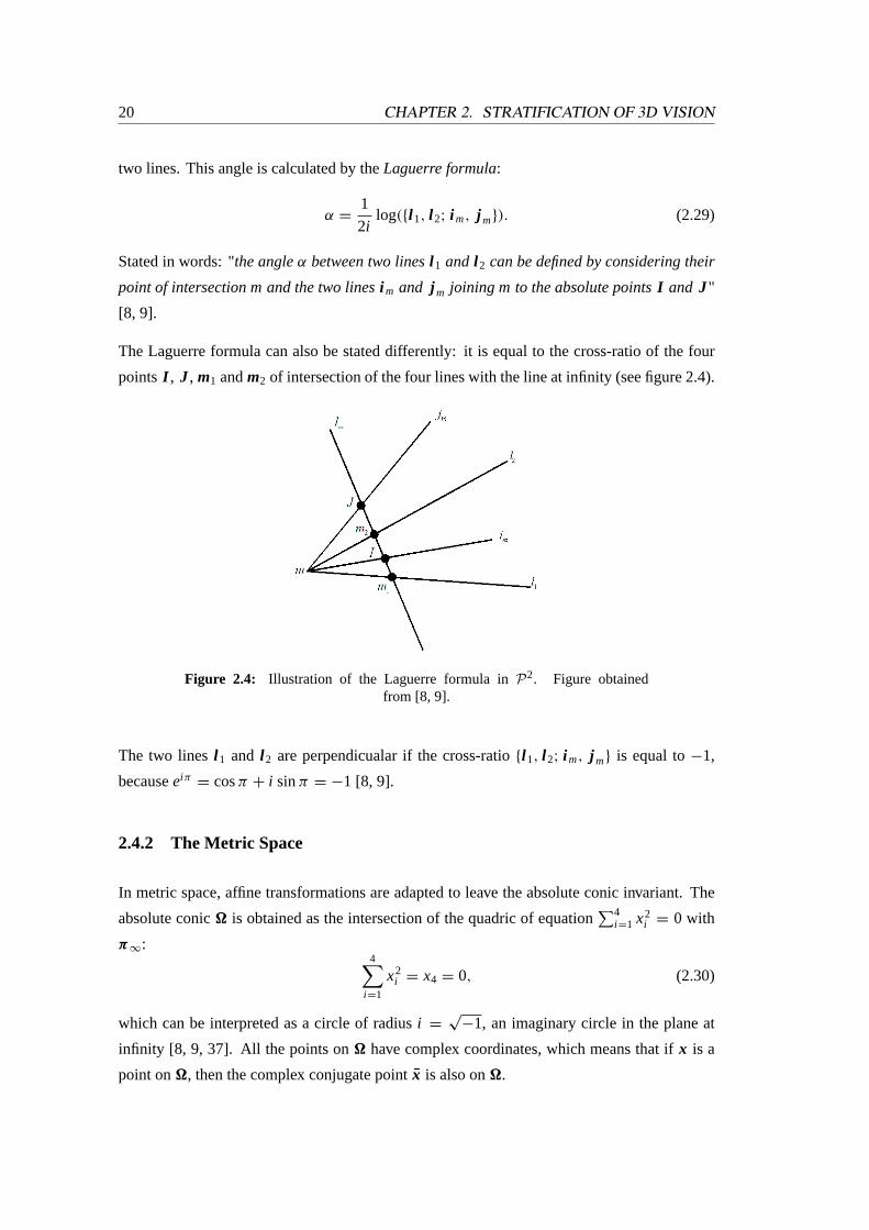
two lines. This angle is calculated by theLaguerre formula:
α =1
2ilog({l 1, l 2; i m, j m}). (2.29)
Stated in words: "the angleα between two linesl 1 and l 2 can be defined by considering their
point of intersectionm and the two linesi m and j m joining m to the absolute pointsI and J"
[8, 9].
The Laguerre formula can also be stated differently: it is equal to the cross-ratio of the four
points I , J , m1 andm2 of intersection of the four lines with the line at infinity (see figure 2.4).
Figure 2.4: Illustration of the Laguerre formula inP2. Figure obtainedfrom [8, 9].
The two linesl 1 and l 2 are perpendicualar if the cross-ratio{l 1, l 2; i m, j m} is equal to−1,
becauseei π= cosπ + i sinπ = −1 [8, 9].
2.4.2 The Metric Space
In metric space, affine transformations are adapted to leave the absolute conic invariant. The
absolute conic� is obtained as the intersection of the quadric of equation∑4
i =1 x2i = 0 with
π∞:4∑
i =1
x2i = x4 = 0, (2.30)
which can be interpreted as a circle of radiusi =√
−1, an imaginary circle in the plane at
infinity [8, 9, 37]. All the points on� have complex coordinates, which means that ifx is a
point on�, then the complex conjugate pointx is also on�.
2.4. METRIC GEOMETRY 21
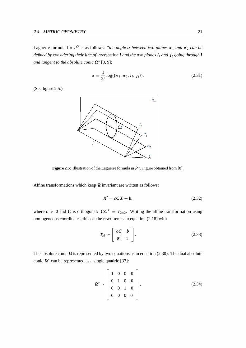
Laguerre formula forP3 is as follows: "the angleα between two planesπ1 and π2 can be
defined by considering their line of intersectionl and the two planesi l and j l going throughl
and tangent to the absolute conic�" [8, 9]:
α =1
2ilog({π1, π2; i l , j l }). (2.31)
(See figure 2.5.)
Figure 2.5: Illustration of the Laguerre formula inP3. Figure obtained from [8].
Affine transformations which keep� invariant are written as follows:
X ′= cC X + b, (2.32)
wherec > 0 andC is orthogonal:CCT= I 3×3. Writing the affine transformation using
homogeneous coordinates, this can be rewritten as in equation (2.18) with
TM ∼
[cC b
0T3 1
]. (2.33)
The absolute conic� is represented by two equations as in equation (2.30). The dual absolute
conic�∗ can be represented as a single quadric [37]:
�∗∼
1 0 0 0
0 1 0 0
0 0 1 0
0 0 0 0
, (2.34)
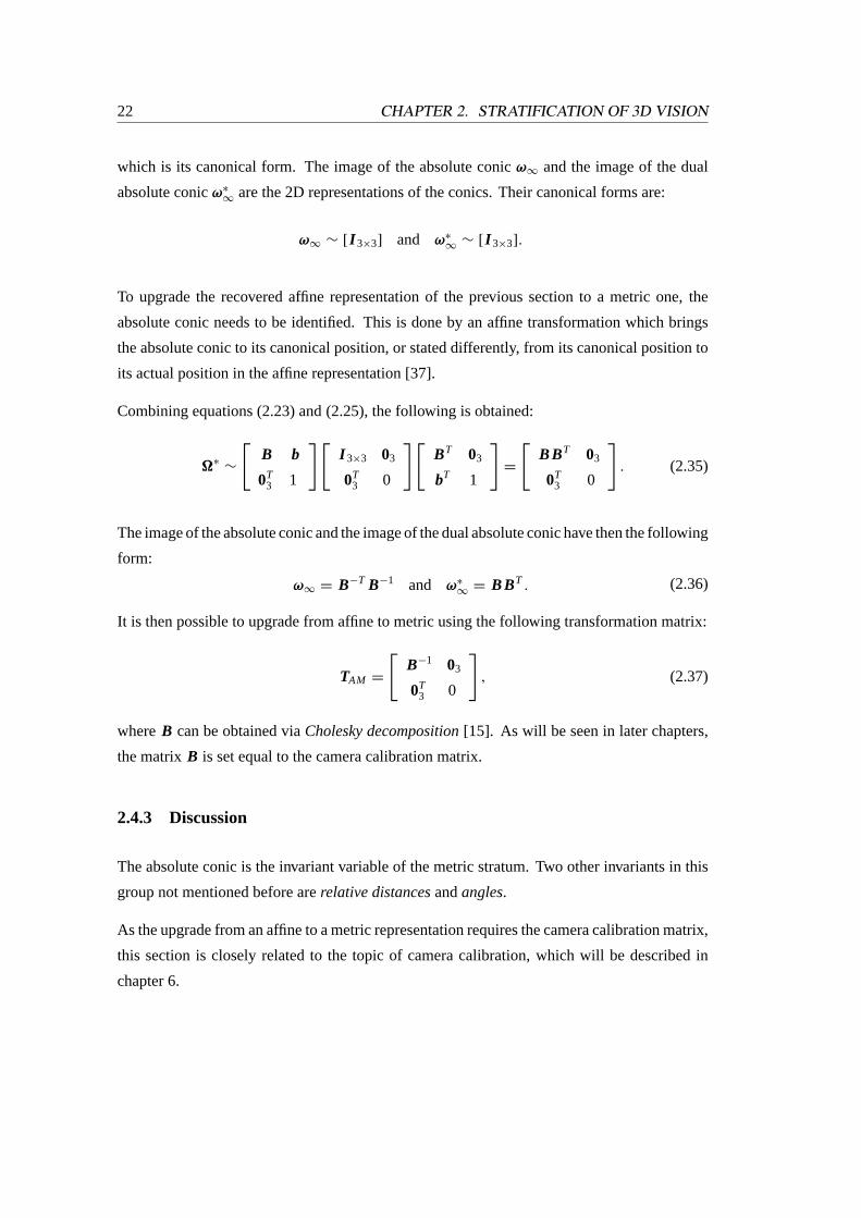
22 CHAPTER 2. STRATIFICATION OF 3D VISION
which is its canonical form. The image of the absolute conicω∞ and the image of the dual
absolute conicω∗
∞are the 2D representations of the conics. Their canonical forms are:
ω∞ ∼ [ I 3×3] and ω∗
∞∼ [ I 3×3].
To upgrade the recovered affine representation of the previous section to a metric one, the
absolute conic needs to be identified. This is done by an affine transformation which brings
the absolute conic to its canonical position, or stated differently, from its canonical position to
its actual position in the affine representation [37].
Combining equations (2.23) and (2.25), the following is obtained:
�∗∼
[B b
0T3 1
][I 3×3 03
0T3 0
][BT 03
bT 1
]=
[BBT 03
0T3 0
]. (2.35)
The image of the absolute conic and the image of the dual absolute conic have then the following
form:
ω∞ = B−T B−1 and ω∗
∞= BBT . (2.36)
It is then possible to upgrade from affine to metric using the following transformation matrix:
TAM =
[B−1 03
0T3 0
], (2.37)
whereB can be obtained viaCholesky decomposition[15]. As will be seen in later chapters,
the matrixB is set equal to the camera calibration matrix.
2.4.3 Discussion
The absolute conic is the invariant variable of the metric stratum. Two other invariants in this
group not mentioned before arerelative distancesandangles.
As the upgrade from an affine to a metric representation requires the camera calibration matrix,
this section is closely related to the topic of camera calibration, which will be described in
chapter 6.
2.5. EUCLIDEAN GEOMETRY 23
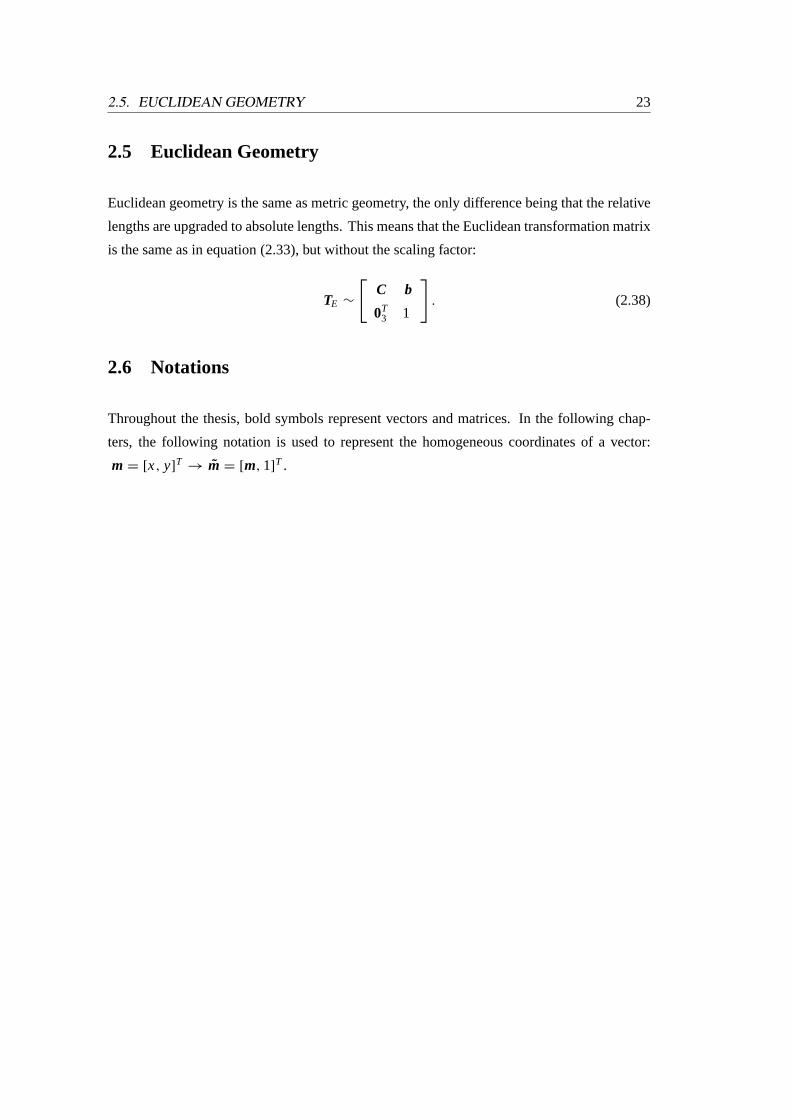
2.5 Euclidean Geometry
Euclidean geometry is the same as metric geometry, the only difference being that the relative
lengths are upgraded to absolute lengths. This means that the Euclidean transformation matrix
is the same as in equation (2.33), but without the scaling factor:
TE ∼
[C b
0T3 1
]. (2.38)
2.6 Notations
Throughout the thesis, bold symbols represent vectors and matrices. In the following chap-
ters, the following notation is used to represent the homogeneous coordinates of a vector:
m = [x, y]T
→ m = [m, 1]T .

24 CHAPTER 2. STRATIFICATION OF 3D VISION
Chapter 3
Camera Model and Epipolar
Geometry
3.1 Introduction
This chapter introduces the camera model and defines theepipolaror two viewgeometry.
A perspective camera model is described in section 3.2, which corresponds to thepinhole
camera. It is assumed throughout this thesis that effects such as radial distortion are negligible
and are thus ignored.
Section 3.3 defines the epipolar geometry that exists between two cameras. A special matrix
will be defined that incorporates the epipolar geometry and forms the building block of the
reconstruction problem.
3.2 Camera Model
A camera is usually described using thepinhole model. As mentioned in section 2.2, there
exists a collineation which maps the projective space to the camera’s retinal plane:P3→ P2.
Then the coordinates of a 3D pointM = [X, Y, Z]T in a Euclidean world coordinate system
and the retinal image coordinatesm = [u, v]T are related by the following equation:
sm = PM , (3.1)
25
26 CHAPTER 3. CAMERA MODEL AND EPIPOLAR GEOMETRY
wheres is a scale factor,m = [u, v, 1]T andM = [X, Y, Z, 1]
T are the homogeneous coordi-
nates of vectorm andM , andP is a 3× 4 matrix representing the collineation:P3→ P2. P
is called the perspective projection matrix.
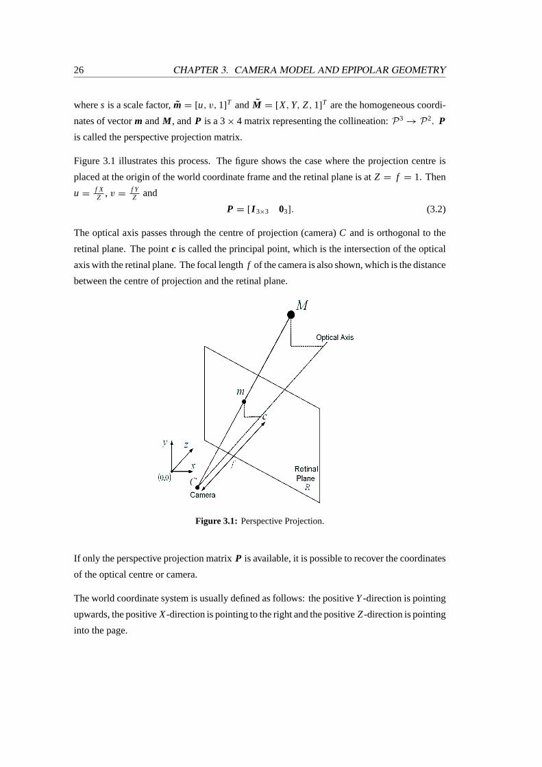
Figure 3.1 illustrates this process. The figure shows the case where the projection centre is
placed at the origin of the world coordinate frame and the retinal plane is atZ = f = 1. Then
u =f XZ , v =
f YZ and
P = [ I 3×3 03]. (3.2)
The optical axis passes through the centre of projection (camera)C and is orthogonal to the
retinal plane. The pointc is called the principal point, which is the intersection of the optical
axis with the retinal plane. The focal lengthf of the camera is also shown, which is the distance
between the centre of projection and the retinal plane.
Figure 3.1: Perspective Projection.
If only the perspective projection matrixP is available, it is possible to recover the coordinates
of the optical centre or camera.
The world coordinate system is usually defined as follows: the positiveY-direction is pointing
upwards, the positiveX-direction is pointing to the right and the positiveZ-direction is pointing
into the page.
3.2. CAMERA MODEL 27
3.2.1 Camera Calibration Matrix
The camera calibration matrix, denoted byK , contains the intrinsic parameters of the camera
used in the imaging process. This matrix is used to convert between the retinal plane and the
actual image plane:
K =
f
pu(tanα)
fpv
u0
0 fpv
v0
0 0 1
. (3.3)
Here, the focal lengthf acts as a scale factor. In a normal camera, the focal length mentioned
above does not usually correspond to 1. It is also possible that the focal length changes during
an entire imaging process, so that for each image the camera calibration matrix needs to be
reestablished.
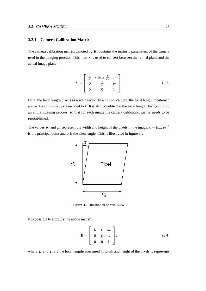
The valuespu and pv represent the width and height of the pixels in the image,c = [u0, v0]T
is the principal point andα is the skew angle. This is illustrated in figure 3.2.
Figure 3.2: Illustration of pixel skew.
It is possible to simplify the above matrix:
K =
fu s u0
0 fv v0
0 0 1
, (3.4)
where fu and fv are the focal lengths measured in width and height of the pixels,s represents
28 CHAPTER 3. CAMERA MODEL AND EPIPOLAR GEOMETRY
the pixel skew and the ratiofu: fv characterises the aspect ratio of the camera.
It is possible to use the camera calibration matrix to transform points from the retinal plane to
points on the image plane:
m = K mR. (3.5)
The estimation of the camera calibration matrix is described in chapter 6.
3.2.2 Camera Motion
Motion in a 3D scene is represented by arotation matrix R and atranslationvector t. The
motion of the camera from coordinateC1 to C2 is then described as follows:
C2 =
[R t
0T3 1
]C1, (3.6)
whereR is the 3× 3 rotation matrix andt the translation in theX-, Y- andZ- directions. The
motion of scene points is equivalent to the inverse motion of the camera (Pollefeys [37] defines
this as the other way around) :
M 2 =
[RT
−RT t
0T3 1
]M 1. (3.7)
Equation (3.1) with equations (3.2), (3.5) and (3.6) then redefine the perspective projection
matrix:
sm = K[
R t]
M , (3.8)
whereP = K[
R t].
3.3 Epipolar Geometry
The epipolar geometry exists between a two camera system. With reference to figure 3.3, the
two cameras are represented byC1 andC2.
Pointsm1 in the first image andm2 in the second image are the imaged points of the 3D point
M . Pointse1 ande2 are the so-calledepipoles, and they are the intersections of the line joining
the two camerasC1 andC2 with both image planes or the projection of the cameras in the
3.3. EPIPOLAR GEOMETRY 29
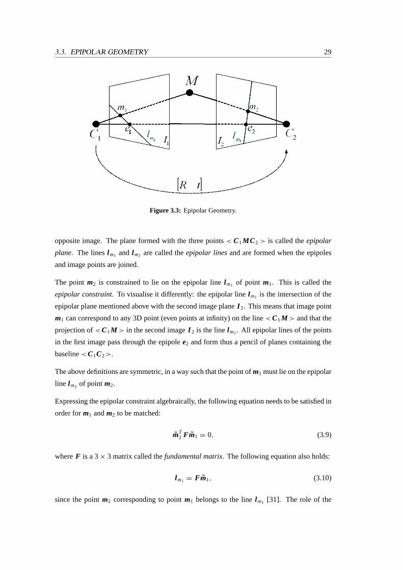
Figure 3.3: Epipolar Geometry.
opposite image. The plane formed with the three points< C1MC2 > is called theepipolar
plane. The linesl m1 and l m2 are called theepipolar linesand are formed when the epipoles
and image points are joined.
The pointm2 is constrained to lie on the epipolar linel m1 of point m1. This is called the
epipolar constraint. To visualise it differently: the epipolar linel m1 is the intersection of the
epipolar plane mentioned above with the second image planeI 2. This means that image point
m1 can correspond to any 3D point (even points at infinity) on the line< C1M > and that the
projection of<C1M > in the second imageI 2 is the linel m1. All epipolar lines of the points
in the first image pass through the epipolee2 and form thus a pencil of planes containing the
baseline<C1C2>.
The above definitions are symmetric, in a way such that the point ofm1 must lie on the epipolar
line l m2 of point m2.
Expressing the epipolar constraint algebraically, the following equation needs to be satisfied in
order form1 andm2 to be matched:
mT2 Fm1 = 0, (3.9)
whereF is a 3× 3 matrix called thefundamental matrix. The following equation also holds:
l m1 = Fm1, (3.10)
since the pointm2 corresponding to pointm1 belongs to the linel m1 [31]. The role of the
30 CHAPTER 3. CAMERA MODEL AND EPIPOLAR GEOMETRY
images can be reversed and then:
mT1 F T m2 = 0,
which shows that the fundamental matrix is changed to its transpose.
Making use of equation (3.8), if the first camera coincides with the world coordinate system
then
s1m1 = K 1
[I 3×3 03
]M
s2m2 = K 2
[R t
]M ,
whereK 1 andK 2 are the camera calibration matrices for each camera, andR andt describe a
transformation (rotation and translation) which brings points expressed in the first coordinate
system to the second one. The fundamental matrix can then be expressed as follows:
F = K−T2 [t]x RK−1
1 , (3.11)
where[t]x is the antisymmetric matrix as described in equation (2.6).
Since det([t]x) = 0, det(F) = 0 and F is of rank 2 [52]. The fundamental matrix is also
only defined up to a scalar factor, and therefore it has seven degrees of freedom (7 independent
parameters among the 9 elements ofF ).
A note on the fundamental matrix: if the intrinsic parameters of the camera are known, such
as in equation (3.11), then the fundamental matrix is called theessential matrix[31].
Another property of the fundamental matrix is derived from equations (3.9) and (3.10):
Fe1 = F T e2 = 0. (3.12)
Clearly, the epipolar line of epipolee1 is Fe1.
Chapter 4
Fundamental Matrix Estimation
4.1 Introduction
The whole 3D reconstruction process relies heavily on a robust estimation of the fundamental
matrix, which is able to detect outliers in the correspondences. This chapter will explain how
the fundamental matrix is calculated using a robust method incorporating both a linear and
nonlinear method. This chapter is based on descriptions by Zhang [50, 52] and by Luong and
Faugeras [31].
As the fundamental matrix has only seven degrees of freedom, it is possible to estimateF
directly using only 7 point matches. In general more than 7 point matches are available and a
method for solving the fundamental matrix using 8 point matches is given in section 4.2. The
points in both images are usually subject to noise and therefore a minimisation technique is
implemented and described in section 4.3. A robust method is described in section 4.4 which
allows for outliers in the list of matches. This is very useful as the technique will ignore these
false matches in the estimation of the fundamental matrix. A short comparison with another
robust method, called RANSAC, is given in section 4.5.
4.2 Linear Least-Squares Technique
Having matched a corner pointm1i = [u1i , v1i ]T in the first image with a corner pointm2i =
[u2i , v2i ]T in the second image, the epipolar equation can be written as follows:
mT2i Fm1i = 0. (4.1)
31
32 CHAPTER 4. FUNDAMENTAL MATRIX ESTIMATION
This equation can be rewritten as a linear and homogeneous equation in the 9 unknown coeffi-
cients of matrixF :
uTi f = 0, (4.2)
where
ui = [u1i u2i , v1i u2i , u2i , u1i v2i , v1i v2i , v2i , u1i , v1i , 1]T
f = [F11, F12, F13, F21, F22, F23, F31, F32, F33]T
andFi j is the element ofF at row i and columnj . If n corner point matches are present and
by stacking equation (4.2), the following linear system is obtained:
Un f = 0,
where
Un = [u1, . . . , un]T .
If 8 or more corner point correspondences are present and ignoring the rank-2 constraint, a
least-squares method can be used to solve
minF
∑i
(mT2i Fm1i )
2, (4.3)
which can be rewritten as:
minf
‖Un f ‖2.
Various methods exists to solve forf . They are called the 8-point algorithms, as 8 or more
points are needed to solve forf . One of the methods sets one of the coefficients ofF to 1 and
then solves equation (4.3) using a linear least-squares technique [52].
A second method imposes a constraint on the norm off (i.e. ‖ f ‖ = 1), and the above linear
system can be solved using Eigen analysis [31, 52, 54]. The solution will then be the unit
eigenvector of matrixUTn Un associated with the smallest eigenvalue, and can be found via
Singular Value Decomposition[15].
The problem with this computation is that it is very sensitive to noise, even when a large number
of matches are present. A reason for this is that therank-2constraint of the fundamental matrix
(i.e. det(F) = 0) is not satisfied [52, 54].
Hartley [18] challenges the view that the 8-point algorithms are very noisy in calculations and
4.3. MINIMISING THE DISTANCES TO EPIPOLAR LINES 33
shows that by normalising the coordinates of the matched points, better results are obtained.
One of the normalisation techniques he is using is non-isotropic scaling, where the centroid of
the points is translated to the origin. After the translation the points form a cloud about the
origin, which is scaled such that it appears to be symmetric circular with a radius of one (the
two principal moments of the set of points are equal to one). The steps of the translation and
scaling are as follows: for all pointsmi , (i, . . . , N), matrix∑
i mi mTi is formed. As this matrix
is symmetric and positive definite,Cholesky decomposition[15] will result in:
N∑i =1
mi mTi = N AAT ,
where matrixA is upper triangular. The above equation can be rewritten:
N∑i =1
A−1mi mTi A−T
= N I ,
whereI is the identity matrix. Settingm′i = A−1mi , the equation for the transformed points
becomes:N∑
i =1
m′i m′T
i = N I .
This shows that the transformed points have their centroid at the origin and the two principal
moments are both equal to one. The above transformation is applied to points in both images,
yielding two transformation matricesA1 and A2.
After estimating the fundamental matrixF ′ corresponding to the normalised point coordinates
using the 8-point algorithm described above, the fundamental matrixF corresponding to the
original unnormalised point coordinates is calculated as follows:
F = AT2 F ′ A1.
4.3 Minimising the Distances to Epipolar Lines
To satisfy therank-2 constraint of the fundamental matrix,F can be written in terms of 7
parameters [52, 50]. ThereforeF can be parameterised as follows:a b −ax1 − by1
c d −cx1 − dy1
−ax2 − cy2 −bx2 − dy2 (ax1 + by1)x2 + (cx1 + dy1)y2
. (4.4)
34 CHAPTER 4. FUNDAMENTAL MATRIX ESTIMATION
The parameters(x1, y1) and(x2, y2) are the coordinates of the two epipolese1 ande2. The
four parameters(a, b, c, d) define the relationship between the orientations of the two pencils
of epipolar lines [50]. The matrix is normalised by dividing the four parameters(a, b, c, d) by
the largest in absolute value.
The fundamental matrix in the previous section is used as an initial guess and to estimate the
two epipoles. The following technique is used by Zhang [50] to calculate the two epipoles. If
M = U DV T
is theSingular Value Decompositionof a matrixM [15], then
D =
d1 0 0
0 d2 0
0 0 d3
is the diagonal matrix satisfyingd1 ≥ d2 ≥ d3 ≥ 0, wheredi is thei th singular value, andU
andV are orthogonal matrices. Then
F = U DV T , (4.5)
where
D =
ds1 0 0
0 d2 0
0 0 0
satisfies therank-2constraint of the fundamental matrix. The epipoles are then calculated from
Fe1 = 0 and F T e2 = 0, (4.6)
wheree1 = [e11, e12, e13]T and e1 = [e21, e22, e23]
T are equal to the last column ofV andU
respectively. Then
xi = ei 1/ei 3 and yi = ei 2/ei 3 for i = 1, 2.
The four parameters(a, b, c, d) are found directly from the fundamental matrixF . Thus the
seven initial parameters are(x1, y1, x2, y2) and three among(a, b, c, d) and the final estimates
are calculated by minimising the sum of distances between corner points and their epipolar
4.4. LEAST-MEDIAN-OF-SQUARES METHOD 35
lines. The following nonlinear equation is minimised:
minF
∑i
d2(m2i , Fm1i ), (4.7)
where
d(m2, Fm1) =|mT
2 Fm1|√(Fm1)
21 + (Fm1)
22
is the Euclidean distance of pointm2 to its epipolar lineFm1, and(Fm1)i is thei th variable
of vectorFm1.
To make the calculation symmetric, equation (4.7) is extended to
minF
∑i
(d2(m2i , Fm1i ) + d2(m1i , F T m2i )
),
which can be rewritten by using the fact thatmT2 Fm1 = mT
1 F T m2:
minF
∑i
(1
(Fm1i )21 + (Fm1i )
22
+1
(F T m2i )21 + (F T m2i )
22
)(mT
2i Fm1i )2. (4.8)
4.4 Least-Median-of-Squares method
The above mentioned methods would introduce inaccuracies into the calculation of the funda-
mental matrix if outliers are present. The method outlined in this section is used in the corner
matching process described in chapter 5 and it has the important ability to detect outliers or
false matches and still give an accurate estimation of the fundamental matrix. This is originally
based on the method outlined in chapter 5 of Rousseeuw and Leroy’s book on regression [41]
and adapted by Zhang et. al. for the fundamental matrix estimation [54, 52].
For n corner point correspondences(m1i , m2i ) as estimated in chapter 5, aMonte Carlotype
technique is used to drawmsubsamples ofp = 8 different corner point correspondences. Then
for each subsamplej the fundamental matrixFj is calculated. The median of squared residuals
(M j ) is determined for eachFj with respect to the whole set of corner point correspondences:
M j = medi =1,...,n[d2(m2i , Fj m1i ) + d2(m1i , F T
j m2i )].
The estimate ofFj , for which M j is minimal among allm Mj ’s, is kept for the next stage of
the algorithm.
36 CHAPTER 4. FUNDAMENTAL MATRIX ESTIMATION
The number of subsamplesm is determined by the following equation:
P = 1 − [1 − (1 − ε)p]m, (4.9)
which calculates the probability that at least one of them subsamples is ‘good’ (a ‘good’
subsample consists ofp good correspondences) and assuming that the whole set of correspon-
dences contains up toε outliers. Zhang et. al. [54] sets the variables as follows: forP = 0.99
and assumingε = 40%,mwill be equal to 272. To compensate for Gaussian noise, Rousseeuw
and Leroy [41] calculate therobust standard deviationestimate
σ = 1.4826[1 + 5/(n − p)]√
M j ,
whereM j is the minimal median.
Based on therobust standard deviationσ , it is possible to assign a weight for each corner
correspondence:
wi =
{1 if r 2
i ≤ (2.5σ )2
0 otherwise,
where
r 2i = d2(m2i , Fm1i ) + d2(m1i , F T m2i ).
The outliers are therefore all the correspondences with weightwi = 0 and are not taken into
account. The fundamental matrix is then finally calculated by solving the weighted least-squares
problem:
min∑
i
wi r2i . (4.10)
All the nonlinear minimisations have been done using theLevenberg-Marquardtalgorithm
[35, 40], described in appendix C.
Bucket Technique
As mentioned before, aMonte Carlotype technique is implemented. A problem with this is
that the eight points generated for each subsample could lie very close to each other which
makes the estimation of the epipolar geometry very inaccurate. In order to achieve a more
reliable result, the followingregularly random selection method, developed by Zhang et. al.
[54], is implemented.
This method is based on bucketing techniques. The minimum and maximum coordinates of
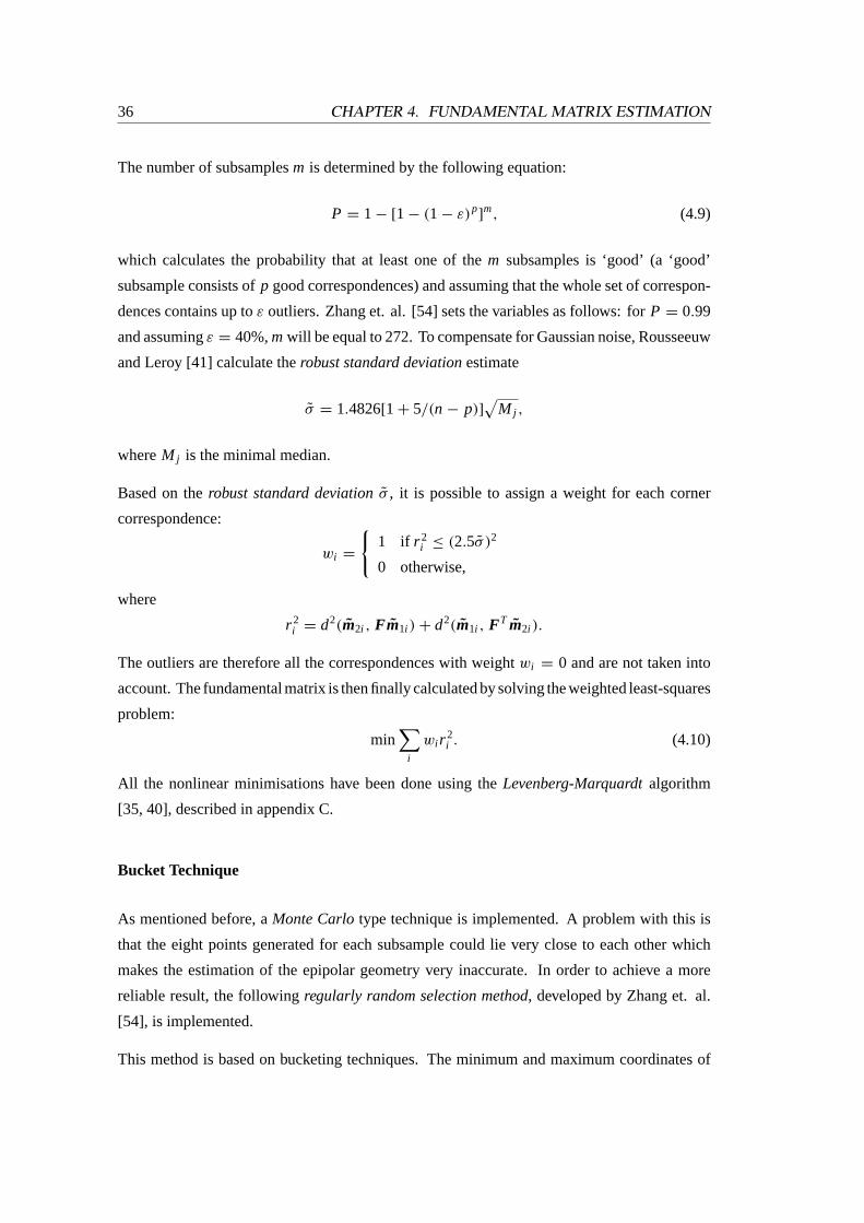
4.4. LEAST-MEDIAN-OF-SQUARES METHOD 37
the corner points in the first image define a region which is divided intob × b buckets, as seen
in figure 4.1.
Figure 4.1: Illustration of bucketing technique.
Each bucket contains a number of corner points and indirectly a set of matches. Buckets
having no matches are ignored. Then to generate a subsample, 8 mutually different buckets
are randomly selected, and then one match is randomly selected in each bucket.
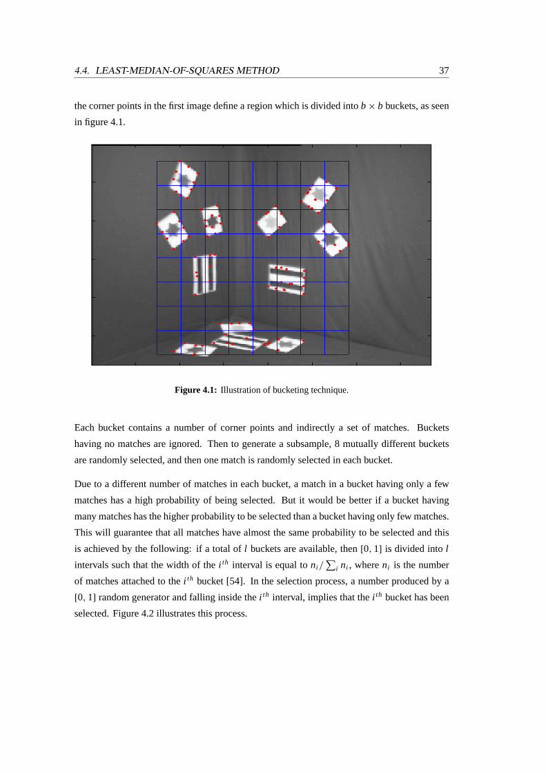
Due to a different number of matches in each bucket, a match in a bucket having only a few
matches has a high probability of being selected. But it would be better if a bucket having
many matches has the higher probability to be selected than a bucket having only few matches.
This will guarantee that all matches have almost the same probability to be selected and this
is achieved by the following: if a total ofl buckets are available, then[0, 1] is divided intol
intervals such that the width of thei th interval is equal toni /∑
i ni , whereni is the number
of matches attached to thei th bucket [54]. In the selection process, a number produced by a
[0, 1] random generator and falling inside thei th interval, implies that thei th bucket has been
selected. Figure 4.2 illustrates this process.
38 CHAPTER 4. FUNDAMENTAL MATRIX ESTIMATION
Figure 4.2: Interval and bucket mapping. Figure obtained from [54].
4.5 RANSAC
RANSAC or random sample consensuswas first used for fundamental matrix estimation by
Torr [47]. It is very similar to the LmedS method described above, a difference being that
a threshold needs to be set by the user to determine if a feature pair is consistent with the
fundamental matrix or not. This threshold is automatically calculated in the LMedS method.
Instead of estimating the median of squared residuals, RANSAC calculates the size of the point
matches that are consistent with eachFj .
Zhang [52] mentions in his paper that if the fundamental matrix needs to be established for
many images, then the LMedS method should be run on one pair of the images to find a suitable
threshold, while RANSAC should be then run on all the remaining images, as RANSAC is able
to terminate once a optimal solution is found and as such runs cheaper.
Chapter 5
Corner Matching
5.1 Introduction
Point matching plays an important part in the estimation of the fundamental matrix. Two
different methods of point matching are introduced and combined to form a robust stereo
matching technique. The first method [54] makes use of correlation techniques followed by
relaxation methods. From these final correspondences, although not all perfect matches, the
optimal fundamental matrix is calculated using theLeast-Median-of-Squaresmethod, which
discards outliers or bad matches. The second method [36] sets up a proximity matrix weighted
by the correlation between matches. Performing a singular value decomposition calculation
on that matrix will ‘amplify’ good pairings and ‘attenuate’ bad ones.
Sections 5.2 and 5.3 of this chapter summarise thecorrelationandstrength of match measure
equations presented in the paper by Zhang et. al. [54], and calculate some correspondence
between the corners in the two images. Section 5.4 describes the SVD algorithm by Pilu [36]
and shows how to combine both methods to get a list of initial matches. In section 5.5 the
stereo matching algorithm by Zhang et. al. [54] is outlined, which resolves false matches and
outliers.
Results are given at the end of this chapter. The matching process works well on images
containing different patterns and textures, and features are matched up perfectly under camera
translation, rotation and zooming. However, if the image contains a repetitive pattern, features
are not matched up at all.
It is impossible to obtain corner points from images that contain scenes with a uniform back-
39
40 CHAPTER 5. CORNER MATCHING
ground. Therefore some markers need to be included in the scene in order to obtain sufficient
corner points.
The corner extraction algorithm is described in appendix A.1.
5.2 Establishing Matches by Correlation
Corner points are represented by the vectormi = [ui , vi ]T in the images. A correlation window
of size(2n + 1) × (2m + 1) is centred at each corner detected in the first of two images. A
rectangular search area of size(2du + 1) × (2dv + 1) is placed around this point in the second
image and for all the corners falling inside this area a correlation score is defined:
Score(m1, m2) =
n∑i =−n
m∑j =−m
[I1(u1 + i, v1 + j ) − I1(u1, v1)
]×
[I2(u2 + i, v2 + j ) − I2(u2, v2)
](2n + 1)(2m + 1)
√σ 2(I1) × σ 2(I2)
,
(5.1)
whereIk(u, v) =∑n
i =−n
∑mj =−m Ik(u + i, v + j )/[(2n + 1)(2m + 1)] is the average at point
(u, v) of Ik(k = 1, 2), andσ(Ik) is the standard deviation of the imageIk in the neighbourhood
(2n + 1) × (2m + 1) of (u, v), which is given by
σ(Ik) =
√∑ni =−n
∑mj =−m I 2
k (u, v)
(2n + 1)(2m + 1)− Ik(u, v). (5.2)
The score ranges from -1 for uncorrelated windows to 1 for identical matches.
Matches above a certain threshold are then selected and form candidate matches. Thus each
corner in the first image is associated with a set of candidate matches from the second image
and vice versa. It is possible that there are no candidate matches for certain corners.
In this implementation,n = m = 7 for the correlation window and the threshold was chosen
to be in the range of 0.7 − 0.8. The search window size,du anddv, was set to an eighth of the
image width and height respectively.
5.3 Support of each Match
This section will define a measure of support for each match, which is called the strength of
the match in [54].
5.3. SUPPORT OF EACH MATCH 41
Each candidate match is written as(m1i , m2 j ), wherem1i is a corner in the first image and
m2 j a corner in the second image. ThenN (m1i ) andN (m2 j ) are the neighbours ofm1i and
m2 j within a disc of radiusR. If (m1i , m2 j ) is a good match, there should be many matches
(n1k, n2l ), wheren1k ∈ N (m1i ) andn2l ∈ N (m2 j ), such that the position ofn1k relative to
m1i is similar to that ofn2l relative tom2 j . If the match is not so good, then there should be
only a few matches in the neighbourhood or none at all.
Thestrength of the matchor S is then defined as:
S(m1i , m2 j ) = ci j
∑n1k∈N (m1i )
[max
n2l ∈N (m2 j )
cklδ(m1i , m2 j ; n1k, n2l )
1 + dist(m1i , m2 j ; n1k, n2l )
], (5.3)
whereci j andckl are the correlation scores of the candidate matches(m1i , m2 j ) and(n1k, n2l )
from the previous section. The average distance between the two pairings is defined as:
dist(m1i , m2 j ; n1k, n2l ) = [d(m1i , n1k) + d(m2 j , n2l )]/2
whered(m, n) = ‖m − n‖ is the Euclidean distance betweenm andn, and
δ(m1i , m2 j ; n1k, n2l ) =
{e−r/εr if (n1k, n2l ) is a candidate match andr < εr
0 otherwise,
with r the relative distance difference given by
r =|d(m1i , n1k) − d(m2 j , n2l )|
dist(m1i , m2 j ; n1k, n2l )
andεr a threshold on the relative distance difference.
The following points clarify the above equations:
• The strength of a match counts the number of candidate matches inside the neighbour-
hoods, but only those whose positions relative to the considered match are similar are
counted.
• The similarity of relative positions is based on the relative distancer . Whenr is very
big, the terme−r/εr →0 and the candidate match(n1k, n2l ) is ignored. Whenr →0, then
e−r/εr →1 and the candidate contributes largely to the match(m1i , m2 j ).
• If a corner point in the first image has several candidate matches in the second image,
the one with the smallest distance difference is chosen as the final one using the ‘max’
operator.
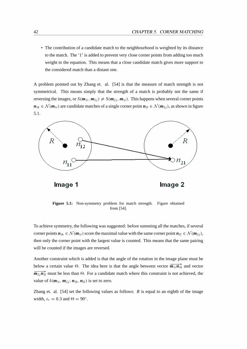
42 CHAPTER 5. CORNER MATCHING
• The contribution of a candidate match to the neighbourhood is weighted by its distance
to the match. The ‘1’ is added to prevent very close corner points from adding too much
weight to the equation. This means that a close candidate match gives more support to
the considered match than a distant one.
A problem pointed out by Zhang et. al. [54] is that the measure of match strength is not
symmetrical. This means simply that the strength of a match is probably not the same if
reversing the images, orS(m1i , m2 j ) 6= S(m2 j , m1i ). This happens when several corner points
n1k ∈ N (m1i ) are candidate matches of a single corner pointn2l ∈ N (m2 j ), as shown in figure
5.1.
Figure 5.1: Non-symmetry problem for match strength. Figure obtainedfrom [54].
To achieve symmetry, the following was suggested: before summing all the matches, if several
corner pointsn1k ∈ N (m1i ) score the maximal value with the same corner pointn2l ∈ N (m2 j ),
then only the corner point with the largest value is counted. This means that the same pairing
will be counted if the images are reversed.
Another constraint which is added is that the angle of the rotation in the image plane must be
below a certain value2. The idea here is that the angle between vector−−−−→m1i n1k and vector−−−−→m2 j n2l must be less than2. For a candidate match where this constraint is not achieved, the
value ofδ(m1i , m2 j ; n1k, n2l ) is set to zero.
Zhang et. al. [54] set the following values as follows:R is equal to an eighth of the image
width, εr = 0.3 and2 = 90◦.
5.4. INITIAL MATCHES BY SINGULAR VALUE DECOMPOSITION 43
5.4 Initial Matches by Singular Value Decomposition
This section explains how initial matches are found viaSingular Value Decomposition, a method
described by Pilu [36] which is originally based on a paper by Scott and Longuet-Higgens [43].
At the end of this section it is shown how this technique can be combined with the strength
measure of section 5.3.
This algorithm complies with Ullman’sminimal mapping theory[48], which states three criteria
for good global mapping:
1. the principle of similarity
2. the principle of proximity
3. the principle of exclusion.
Theprinciple of similarityis an indication of how closely related the corner matches are. The
principle of proximitystates simply that if various corner matches are similar or equal, take
the match which has the shortest distance between the two corner points. For theprincipal of
exclusion, only a one-to-one mapping is allowed between corners.
The algorithm by Scott and Longuet-Higgins [43] will be extended to satisfy all these con-
straints.
The basic algorithm satisfies only the principle of proximity and exclusion. Having corner
pointsm1i (i = 1 . . . m) in the first image andm2 j ( j = 1 . . . n) in the second image, aproximity
matrix is set up as follows:
Gi j = e−r 2i j /2σ2
i = 1 . . . m, j = 1 . . . n (5.4)
wherer i j = ‖m1i − m2 j ‖ is the Euclidean distance between the corner points if they are
regarded of lying on the same plane.Gi j decreases from 1 to 0 with distance. The parameterσ
controls the interaction between features: a small value ofσ enforces local interactions while
a large value allows for more global interactions.
The next stage of the algorithm is to performSingular Value Decomposition(SVD) [15] of G:
G = U DV T ,
whereU andV are orthogonal matrices andD is the diagonal matrix containing the singular
44 CHAPTER 5. CORNER MATCHING
values along the diagonal elementsDi i in descending order.
The diagonal matrixD is then converted to a new matrixE which is obtained by replacing
every diagonal element ofD by a 1. Performing the following operation will then result in a
new proximity matrixP:
P = U EV T .
The matrix P has the same shape asG, but it has the property of pairing up good matches.
Quoting Scott and Longuet-Higgens [43]:
"If Pi j is the greatest element in rowi but not the greatest in columnj , then we
may regardm1i as competing unsuccessfully for partnership withm2 j ; similar
remarks apply ifPi j is the greatest element in its column but not in its row. But if
Pi j is both the greatest element in its row and the greatest element in its column
then we regard those features as being in 1:1 correspondence with one another".
Theprinciple of proximityarises from the nature of theproximity matrixand theprinciple of
exclusionarises due to the orthogonality of matrixP. The squares of the elements in each row
of P can be added up to 1 and this implies that featurem1i cannot be strongly associated with
more than one featurem2 j [43].
To include theprinciple of similarity in the above algorithm, Pilu [36] adds in a measure of
similarity, which is identical to the correlation score calculated in section 5.2. This is done in
the following way:
Gi j =[(ci j + 1)/2
]e−r 2
i j /2σ2(5.5)
whereci j is the correlation score defined in section 5.2. MatrixG is now called acorrelation-
weighted proximity matrixand still ranges from 0 to 1. The better the correlation between two
features, the higher the value ofGi j .
A great advantage of this algorithm is that it performs well when only a few features are
available. Other algorithms, like the one described in Zhang et. al. [54], need many uniformly
distributed features to be able to work properly. A disadvantage is the computational complexity
and cost of the SVD for very large matrices. The implementation here makes use of only a
maximum of 500 corners per image, which limits the proximity matrix to about 500× 500
values.
At the end of his paper, Pilu [36] also suggests incorporating the strength of the match, as
calculated in section 5.3, in the above algorithm. This could be achieved in various ways,
5.5. RESOLVING FALSE MATCHES 45
either in place of the correlation score or in conjunction with equation (5.5).
Here we use the latter idea, and the following is an outline of how equation (5.5) is combined
with the strength measure to select ‘good’ initial matches. Basically three criteria have to be
met. If
1. Pi j is the greatest element in both row and column,
2. ci j is greater than some correlation threshold (≈ 0.7),
3. and the considered match(i, j ) has the greatest strength,
then this match will be included in the list of initial matches.
In effect, the above procedure replaces the relaxation process of Zhang et. al. [54], which
consists of minimising an energy function summing up the strengths of all candidate matches.
5.5 Resolving False Matches
The method described in this section makes use of the epipolar geometry which exists between
the two images in helping to resolve false matches. The fundamental matrix is calculated
on the initial matched points estimated in section 5.4. The method used to calculate the
fundamental matrix is theLeast-Median-of-Squares(LMedS) method described in section 4.4,
which discards false matches or outliers.
The initial matching algorithm described in sections 5.2 to 5.4 is then rerun on all corner points
in both images, but the search window of section 5.2 is replaced by the epipolar constraint in
the following way: the epipolar line for each corner point in the first image is calculated. If
pi = [ ui vi 1 ]
is a corner point in the first image in homogeneous coordinates, then its epipolar line is defined
by
l i = F pi ,
whereF is the fundamental matrix. Then the matched corner in the second image should, if it
is a perfect match, lie on the epipolar line in the second image. A threshold determines whether
possible points should be accepted or discarded. This threshold is in the form of a narrow band
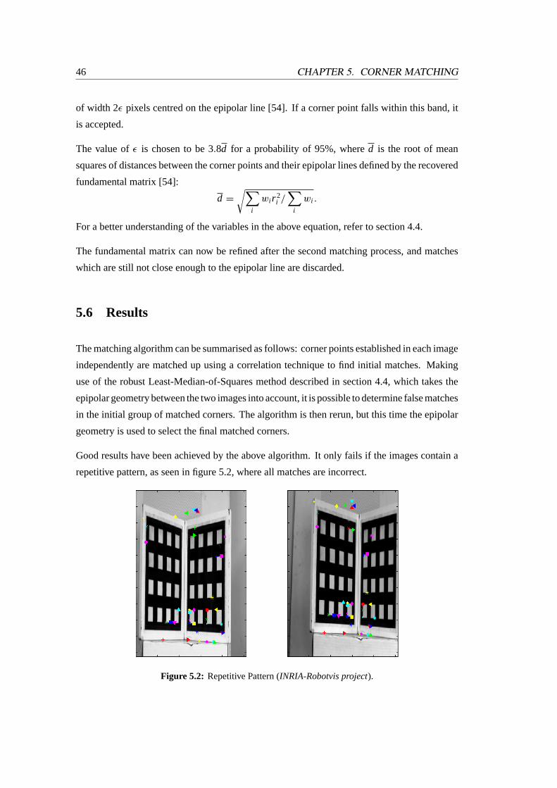
46 CHAPTER 5. CORNER MATCHING
of width 2ε pixels centred on the epipolar line [54]. If a corner point falls within this band, it
is accepted.
The value ofε is chosen to be 3.8d for a probability of 95%, whered is the root of mean
squares of distances between the corner points and their epipolar lines defined by the recovered
fundamental matrix [54]:
d =
√∑i
wi r 2i /∑
i
wi .
For a better understanding of the variables in the above equation, refer to section 4.4.
The fundamental matrix can now be refined after the second matching process, and matches
which are still not close enough to the epipolar line are discarded.
5.6 Results
The matching algorithm can be summarised as follows: corner points established in each image
independently are matched up using a correlation technique to find initial matches. Making
use of the robust Least-Median-of-Squares method described in section 4.4, which takes the
epipolar geometry between the two images into account, it is possible to determine false matches
in the initial group of matched corners. The algorithm is then rerun, but this time the epipolar
geometry is used to select the final matched corners.
Good results have been achieved by the above algorithm. It only fails if the images contain a
repetitive pattern, as seen in figure 5.2, where all matches are incorrect.
Figure 5.2: Repetitive Pattern (INRIA-Robotvis project).

5.6. RESULTS 47
Due to the fact that all corners of the checkered pattern have nearly the same correlation, it
is nearly impossible to match up the corners perfectly. The corner points in each image are
represented by a specific pattern and colour. In this way matched points are easily identified.
Better results can be achieved with a repetitive pattern if it is placed in a scene containing
different structures and patterns.
For a scene with a uniform background, some markers need to be put up in order to find
corresponding corners. This is seen in figure 5.3(a). Here all corners have been perfectly
matched. Figure 5.3(b) shows the camera translation (arrows point to the right) between the
two images. The matching algorithm also has a 100% success rate for the same scene under
camera rotation (arrows point in clockwise direction) and zooming (arrows point inwards), as
seen in figure 5.4 and 5.5.
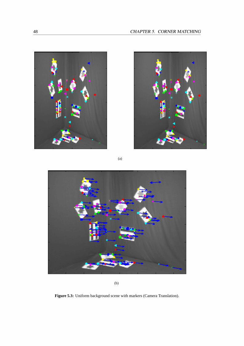
48 CHAPTER 5. CORNER MATCHING
(a)
(b)
Figure 5.3: Uniform background scene with markers (Camera Translation).
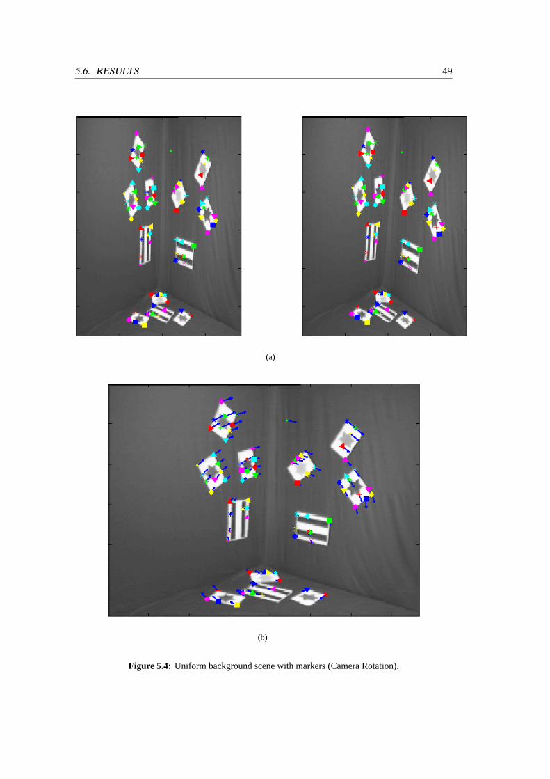
5.6. RESULTS 49
(a)
(b)
Figure 5.4: Uniform background scene with markers (Camera Rotation).
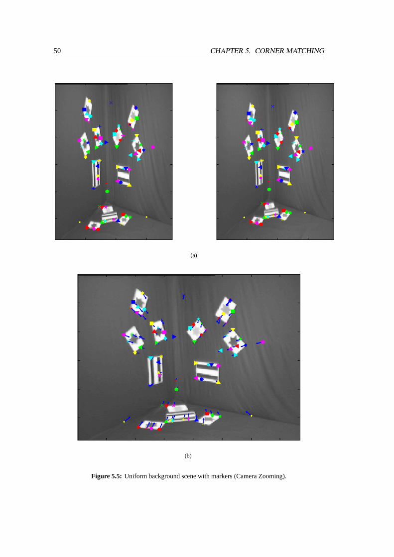
50 CHAPTER 5. CORNER MATCHING
(a)
(b)
Figure 5.5: Uniform background scene with markers (Camera Zooming).
Chapter 6
Camera Calibration
6.1 Introduction
This chapter covers various camera calibration techniques.
Calibration is a fundamental property of 3D reconstruction. Usually the internal parameters
of each camera are very accurately known beforehand and the whole environment is highly
controlled, or a calibration object in the scene is used to calibrate the camera. But in many
situations the source of the images is not known, which means that the camera’s internal
parameters are also not known, or it is desirable to change a camera midway through an image
application. This means that the internal parameters of the camera can only be extracted from
the images themselves.
Section 6.2 gives a background to calibration, explaining original calibration methods. Section
6.3 describes camera selfcalibration and the theory behindKruppa’s equations. In section 6.4
selfcalibration is explained in terms of scene and auto-calibration constraints from only a single
image.
A planar object is used in section 6.5 to estimate the camera calibration matrix. The planar
pattern consists of a grid pattern, which is imaged from different points of view. From each
view, corner points are extracted in order to calculate the correspondence between the image
plane and the planar object. The correspondence is in the form of a homography matrix. Then
for each view, a homography is established and allows for camera calibration.
51
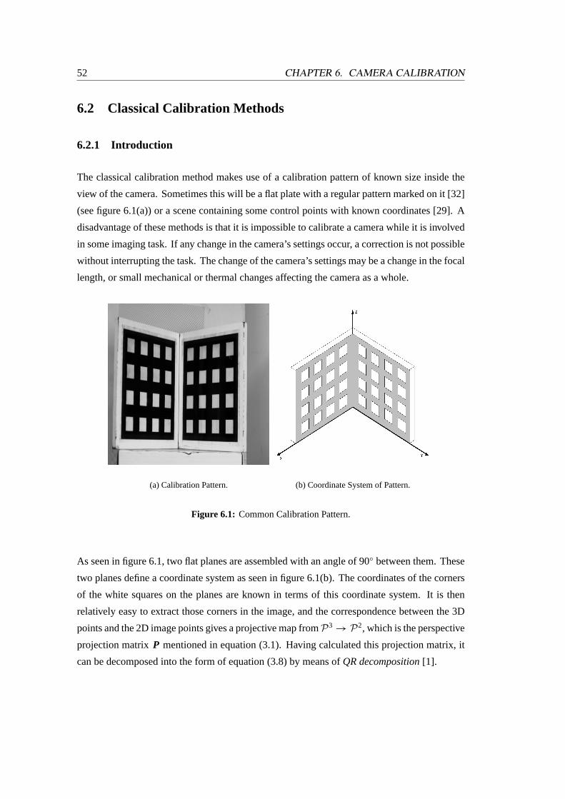
52 CHAPTER 6. CAMERA CALIBRATION
6.2 Classical Calibration Methods
6.2.1 Introduction
The classical calibration method makes use of a calibration pattern of known size inside the
view of the camera. Sometimes this will be a flat plate with a regular pattern marked on it [32]
(see figure 6.1(a)) or a scene containing some control points with known coordinates [29]. A
disadvantage of these methods is that it is impossible to calibrate a camera while it is involved
in some imaging task. If any change in the camera’s settings occur, a correction is not possible
without interrupting the task. The change of the camera’s settings may be a change in the focal
length, or small mechanical or thermal changes affecting the camera as a whole.
(a) Calibration Pattern. (b) Coordinate System of Pattern.
Figure 6.1: Common Calibration Pattern.
As seen in figure 6.1, two flat planes are assembled with an angle of 90◦ between them. These
two planes define a coordinate system as seen in figure 6.1(b). The coordinates of the corners
of the white squares on the planes are known in terms of this coordinate system. It is then
relatively easy to extract those corners in the image, and the correspondence between the 3D
points and the 2D image points gives a projective map fromP3→ P2, which is the perspective
projection matrixP mentioned in equation (3.1). Having calculated this projection matrix, it
can be decomposed into the form of equation (3.8) by means ofQR decomposition[1].
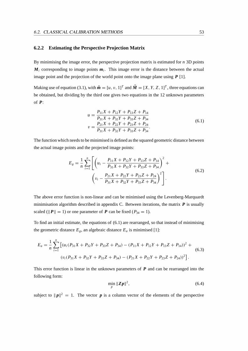
6.2. CLASSICAL CALIBRATION METHODS 53
6.2.2 Estimating the Perspective Projection Matrix
By minimising the image error, the perspective projection matrix is estimated forn 3D points
M i corresponding to image pointsmi . This image error is the distance between the actual
image point and the projection of the world point onto the image plane usingP [1].
Making use of equation (3.1), withm = [u, v, 1]T andM = [X, Y, Z, 1]
T , three equations can
be obtained, but dividing by the third one gives two equations in the 12 unknown parameters
of P:
u =P11X + P12Y + P13Z + P14
P31X + P32Y + P33Z + P34
v =P21X + P22Y + P23Z + P24
P31X + P32Y + P33Z + P34.
(6.1)
The function which needs to be minimised is defined as the squared geometric distance between
the actual image points and the projected image points:
Eg =1
n
n∑i =1
[(ui −
P11X + P12Y + P13Z + P14
P31X + P32Y + P33Z + P34
)2
+
(vi −
P21X + P22Y + P23Z + P24
P31X + P32Y + P33Z + P34
)2]
.
(6.2)
The above error function is non-linear and can be minimised using the Levenberg-Marquardt
minimisation algorithm described in appendix C. Between iterations, the matrixP is usually
scaled (‖P‖ = 1) or one parameter ofP can be fixed (P34 = 1).
To find an initial estimate, the equations of (6.1) are rearranged, so that instead of minimising
the geometric distanceEg, an algebraic distanceEa is minimised [1]:
Ea =1
n
n∑i =1
[(ui (P31X + P32Y + P33Z + P34) − (P11X + P12Y + P13Z + P14))
2+
(vi (P31X + P32Y + P33Z + P34) − (P21X + P22Y + P23Z + P24))2] . (6.3)
This error function is linear in the unknown parameters ofP and can be rearranged into the
following form:
minp
‖Zp‖2, (6.4)
subject to‖ p‖2
= 1. The vectorp is a column vector of the elements of the perspective
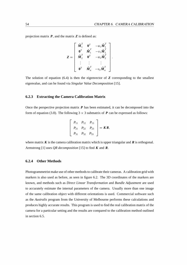
54 CHAPTER 6. CAMERA CALIBRATION
projection matrixP, and the matrixZ is defined as:
Z =
MT1 0T
−u1MT1
0T MT1 −v1M
T1
MT2 0T
−u2MT2
......
...
0T MTn −vnM
Tn
.
The solution of equation (6.4) is then the eigenvector ofZ corresponding to the smallest
eigenvalue, and can be found viaSingular Value Decomposition[15].
6.2.3 Extracting the Camera Calibration Matrix
Once the perspective projection matrixP has been estimated, it can be decomposed into the
form of equation (3.8). The following 3× 3 submatrix ofP can be expressed as follows:P11 P12 P13
P21 P22 P23
P31 P32 P33
= K R,
where matrixK is the camera calibration matrix which is upper triangular andR is orthogonal.
Armstrong [1] usesQR decomposition[15] to find K andR.
6.2.4 Other Methods
Photogrammetrist make use of other methods to calibrate their cameras. A calibration grid with
markers is also used as before, as seen in figure 6.2. The 3D coordinates of the markers are
known, and methods such asDirect Linear TransformationandBundle Adjustmentare used
to accurately estimate the internal parameters of the camera. Usually more than one image
of the same calibration object with different orientations is used. Commercial software such
as theAustralisprogram from the University of Melbourne performs these calculations and
produces highly accurate results. This program is used to find the real calibration matrix of the
camera for a particular setting and the results are compared to the calibration method outlined
in section 6.5.
6.3. SELFCALIBRATION USING KRUPPA’S EQUATIONS 55
Figure 6.2: Six images of a calibration object from the department of geomaticsat UCT.
6.3 Selfcalibration using Kruppa’s Equations
6.3.1 Introduction
In the case of selfcalibration, the known object in the scene is replaced by an abstract object, the
absolute conicmentioned in chapter 2. The absolute conic is a particular conic in the plane of
infinity, which is invariant to transformations of 3D space (see figure 6.3). This means that the
image of the absolute conicω∞ is independent of the position and orientation of the camera.
In figure 6.3, if the camera moves from positionC1 to positionC2 and provided the internal
parameters of the camera stay constant, the image of the absolute conic will be the same in
both image planes.
The image of the absolute conic is related to the camera calibration matrix in the following
way:
ω∞ = K−T K−1. (6.5)
The calibration matrix can then be extracted fromω∞ by Cholesky decomposition[15]. Thus
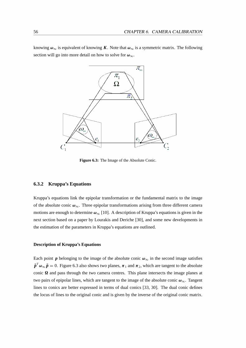
56 CHAPTER 6. CAMERA CALIBRATION
knowingω∞ is equivalent of knowingK . Note thatω∞ is a symmetric matrix. The following
section will go into more detail on how to solve forω∞.
Figure 6.3: The Image of the Absolute Conic.
6.3.2 Kruppa’s Equations
Kruppa’s equations link the epipolar transformation or the fundamental matrix to the image
of the absolute conicω∞. Three epipolar transformations arising from three different camera
motions are enough to determineω∞ [10]. A description of Kruppa’s equations is given in the
next section based on a paper by Lourakis and Deriche [30], and some new developments in
the estimation of the parameters in Kruppa’s equations are outlined.
Description of Kruppa’s Equations
Each pointp belonging to the image of the absolute conicω∞ in the second image satisfies
pTω∞ p = 0. Figure 6.3 also shows two planes,π1 andπ2, which are tangent to the absolute
conic� and pass through the two camera centres. This plane intersects the image planes at
two pairs of epipolar lines, which are tangent to the image of the absolute conicω∞. Tangent
lines to conics are better expressed in terms of dual conics [33, 30]. The dual conic defines
the locus of lines to the original conic and is given by the inverse of the original conic matrix.
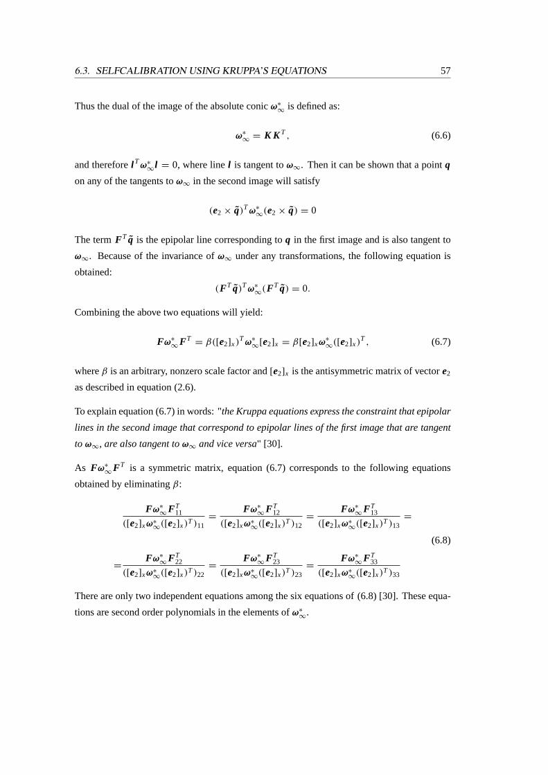
6.3. SELFCALIBRATION USING KRUPPA’S EQUATIONS 57
Thus the dual of the image of the absolute conicω∗
∞is defined as:
ω∗
∞= K K T , (6.6)
and thereforel Tω∗
∞l = 0, where linel is tangent toω∞. Then it can be shown that a pointq
on any of the tangents toω∞ in the second image will satisfy
(e2 × q)Tω∗
∞(e2 × q) = 0
The termF T q is the epipolar line corresponding toq in the first image and is also tangent to
ω∞. Because of the invariance ofω∞ under any transformations, the following equation is
obtained:
(F T q)Tω∗
∞(F T q) = 0.
Combining the above two equations will yield:
Fω∗
∞F T
= β([e2]x)Tω∗
∞[e2]x = β[e2]xω
∗
∞([e2]x)
T , (6.7)
whereβ is an arbitrary, nonzero scale factor and[e2]x is the antisymmetric matrix of vectore2
as described in equation (2.6).
To explain equation (6.7) in words: "the Kruppa equations express the constraint that epipolar
lines in the second image that correspond to epipolar lines of the first image that are tangent
to ω∞, are also tangent toω∞ and vice versa" [30].
As Fω∗
∞F T is a symmetric matrix, equation (6.7) corresponds to the following equations
obtained by eliminatingβ:
Fω∗
∞F T
11
([e2]xω∗∞
([e2]x)T )11=
Fω∗
∞F T
12
([e2]xω∗∞
([e2]x)T )12=
Fω∗
∞F T
13
([e2]xω∗∞
([e2]x)T )13=
=Fω∗
∞F T
22
([e2]xω∗∞
([e2]x)T )22=
Fω∗
∞F T
23
([e2]xω∗∞
([e2]x)T )23=
Fω∗
∞F T
33
([e2]xω∗∞
([e2]x)T )33
(6.8)
There are only two independent equations among the six equations of (6.8) [30]. These equa-
tions are second order polynomials in the elements ofω∗
∞.
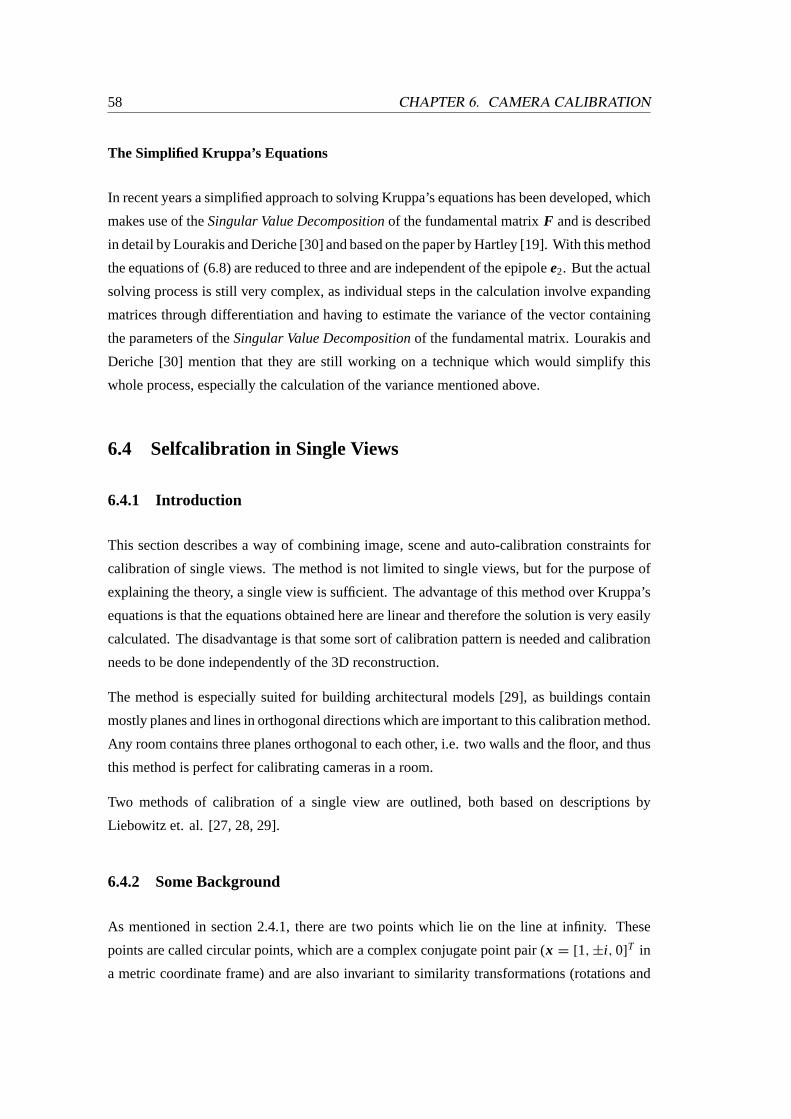
58 CHAPTER 6. CAMERA CALIBRATION
The Simplified Kruppa’s Equations
In recent years a simplified approach to solving Kruppa’s equations has been developed, which
makes use of theSingular Value Decompositionof the fundamental matrixF and is described
in detail by Lourakis and Deriche [30] and based on the paper by Hartley [19]. With this method
the equations of (6.8) are reduced to three and are independent of the epipolee2. But the actual
solving process is still very complex, as individual steps in the calculation involve expanding
matrices through differentiation and having to estimate the variance of the vector containing
the parameters of theSingular Value Decompositionof the fundamental matrix. Lourakis and
Deriche [30] mention that they are still working on a technique which would simplify this
whole process, especially the calculation of the variance mentioned above.
6.4 Selfcalibration in Single Views
6.4.1 Introduction
This section describes a way of combining image, scene and auto-calibration constraints for
calibration of single views. The method is not limited to single views, but for the purpose of
explaining the theory, a single view is sufficient. The advantage of this method over Kruppa’s
equations is that the equations obtained here are linear and therefore the solution is very easily
calculated. The disadvantage is that some sort of calibration pattern is needed and calibration
needs to be done independently of the 3D reconstruction.
The method is especially suited for building architectural models [29], as buildings contain
mostly planes and lines in orthogonal directions which are important to this calibration method.
Any room contains three planes orthogonal to each other, i.e. two walls and the floor, and thus
this method is perfect for calibrating cameras in a room.
Two methods of calibration of a single view are outlined, both based on descriptions by
Liebowitz et. al. [27, 28, 29].
6.4.2 Some Background
As mentioned in section 2.4.1, there are two points which lie on the line at infinity. These
points are called circular points, which are a complex conjugate point pair (x = [1, ±i, 0]T in
a metric coordinate frame) and are also invariant to similarity transformations (rotations and
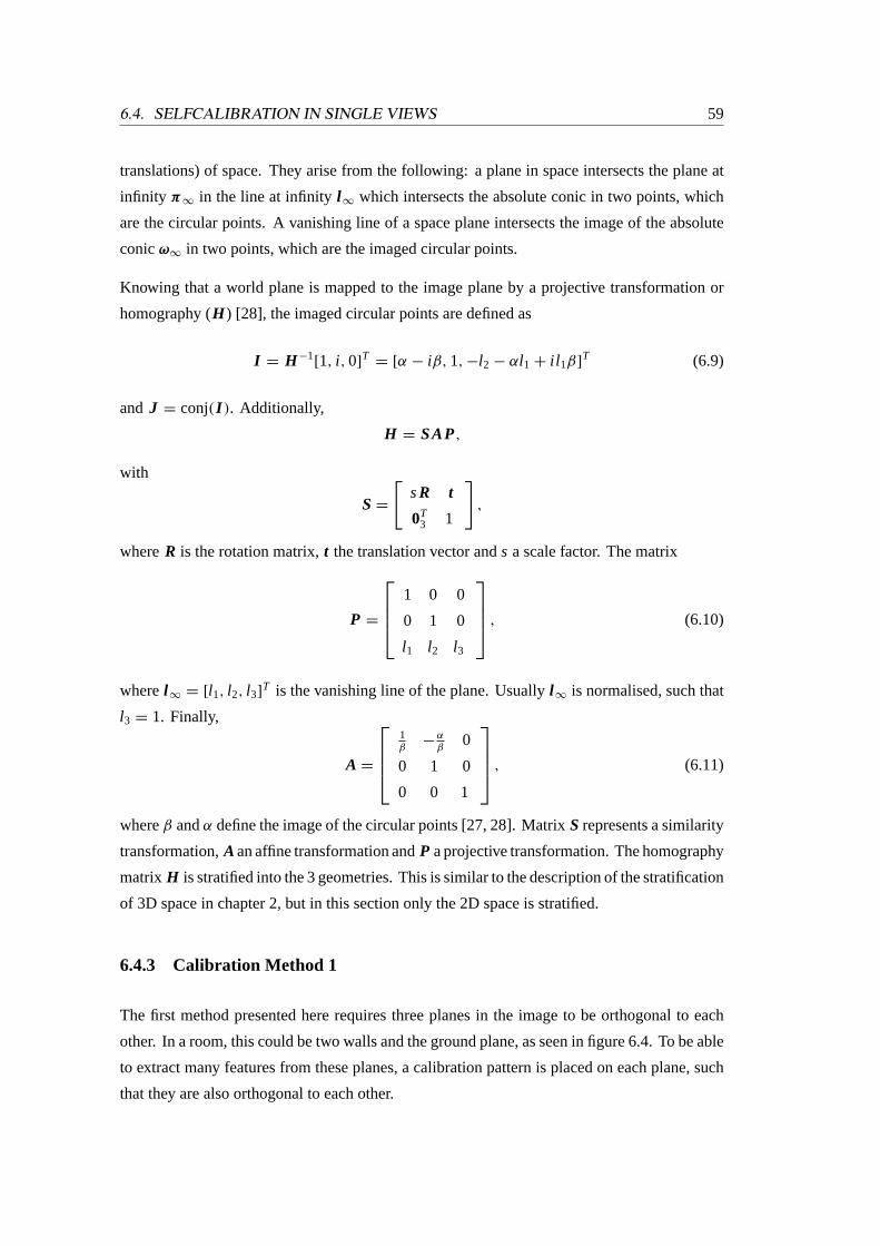
6.4. SELFCALIBRATION IN SINGLE VIEWS 59
translations) of space. They arise from the following: a plane in space intersects the plane at
infinity π∞ in the line at infinityl ∞ which intersects the absolute conic in two points, which
are the circular points. A vanishing line of a space plane intersects the image of the absolute
conicω∞ in two points, which are the imaged circular points.
Knowing that a world plane is mapped to the image plane by a projective transformation or
homography (H ) [28], the imaged circular points are defined as
I = H −1[1, i, 0]
T= [α − iβ, 1, −l2 − αl1 + i l 1β]
T (6.9)
and J = conj( I ). Additionally,
H = SAP,
with
S =
[sR t
0T3 1
],
whereR is the rotation matrix,t the translation vector ands a scale factor. The matrix
P =
1 0 0
0 1 0
l1 l2 l3
, (6.10)
wherel ∞ = [l1, l2, l3]T is the vanishing line of the plane. Usuallyl ∞ is normalised, such that
l3 = 1. Finally,
A =
1β
−αβ
0
0 1 0
0 0 1
, (6.11)
whereβ andα define the image of the circular points [27, 28]. MatrixS represents a similarity
transformation,A an affine transformation andP a projective transformation. The homography
matrix H is stratified into the 3 geometries. This is similar to the description of the stratification
of 3D space in chapter 2, but in this section only the 2D space is stratified.
6.4.3 Calibration Method 1
The first method presented here requires three planes in the image to be orthogonal to each
other. In a room, this could be two walls and the ground plane, as seen in figure 6.4. To be able
to extract many features from these planes, a calibration pattern is placed on each plane, such
that they are also orthogonal to each other.
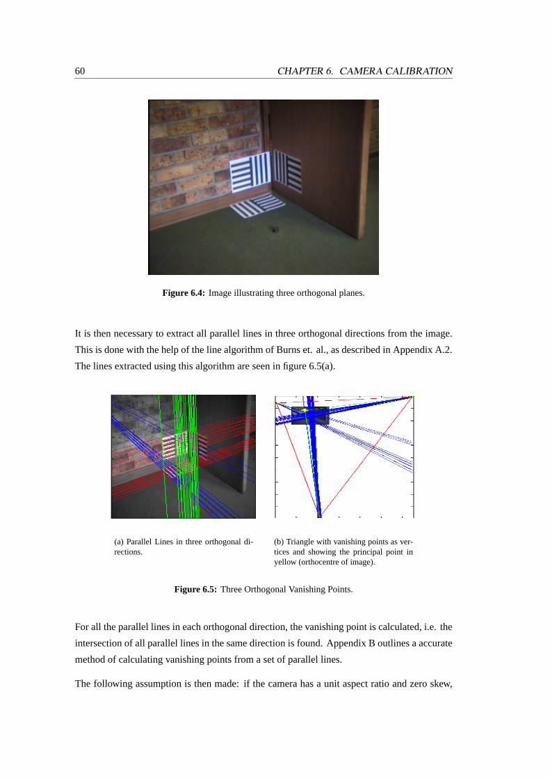
60 CHAPTER 6. CAMERA CALIBRATION
Figure 6.4: Image illustrating three orthogonal planes.
It is then necessary to extract all parallel lines in three orthogonal directions from the image.
This is done with the help of the line algorithm of Burns et. al., as described in Appendix A.2.
The lines extracted using this algorithm are seen in figure 6.5(a).
(a) Parallel Lines in three orthogonal di-rections.
(b) Triangle with vanishing points as ver-tices and showing the principal point inyellow (orthocentre of image).
Figure 6.5: Three Orthogonal Vanishing Points.
For all the parallel lines in each orthogonal direction, the vanishing point is calculated, i.e. the
intersection of all parallel lines in the same direction is found. Appendix B outlines a accurate
method of calculating vanishing points from a set of parallel lines.
The following assumption is then made: if the camera has a unit aspect ratio and zero skew,
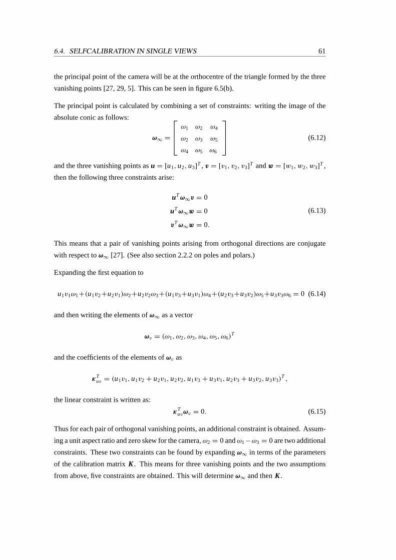
6.4. SELFCALIBRATION IN SINGLE VIEWS 61
the principal point of the camera will be at the orthocentre of the triangle formed by the three
vanishing points [27, 29, 5]. This can be seen in figure 6.5(b).
The principal point is calculated by combining a set of constraints: writing the image of the
absolute conic as follows:
ω∞ =
ω1 ω2 ω4
ω2 ω3 ω5
ω4 ω5 ω6
(6.12)
and the three vanishing points asu = [u1, u2, u3]T , v = [v1, v2, v3]
T andw = [w1, w2, w3]T ,
then the following three constraints arise:
uTω∞v = 0
uTω∞w = 0
vTω∞w = 0.
(6.13)
This means that a pair of vanishing points arising from orthogonal directions are conjugate
with respect toω∞ [27]. (See also section 2.2.2 on poles and polars.)
Expanding the first equation to
u1v1ω1+(u1v2+u2v1)ω2+u2v2ω3+(u1v3+u3v1)ω4+(u2v3+u3v2)ω5+u3v3ω6 = 0 (6.14)
and then writing the elements ofω∞ as a vector
ωv = (ω1, ω2, ω3, ω4, ω5, ω6)T
and the coefficients of the elements ofωv as
κTuv = (u1v1, u1v2 + u2v1, u2v2, u1v3 + u3v1, u2v3 + u3v2, u3v3)
T ,
the linear constraint is written as:
κTuvωv = 0. (6.15)
Thus for each pair of orthogonal vanishing points, an additional constraint is obtained. Assum-
ing a unit aspect ratio and zero skew for the camera,ω2 = 0 andω1−ω3 = 0 are two additional
constraints. These two constraints can be found by expandingω∞ in terms of the parameters
of the calibration matrixK . This means for three vanishing points and the two assumptions
from above, five constraints are obtained. This will determineω∞ and thenK .
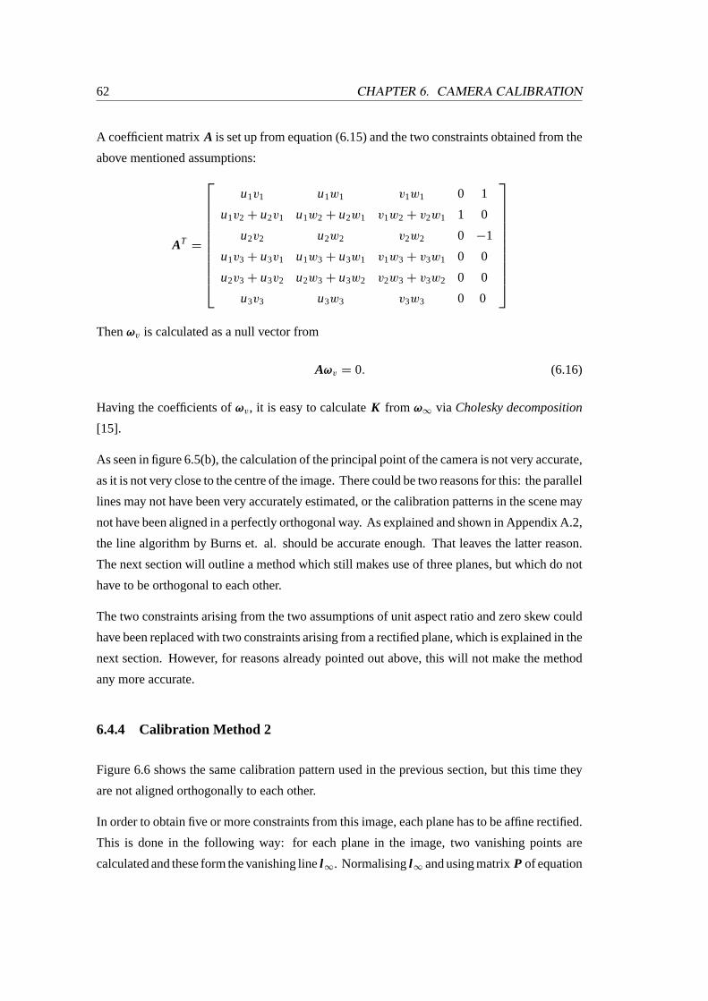
62 CHAPTER 6. CAMERA CALIBRATION
A coefficient matrixA is set up from equation (6.15) and the two constraints obtained from the
above mentioned assumptions:
AT=
u1v1 u1w1 v1w1 0 1
u1v2 + u2v1 u1w2 + u2w1 v1w2 + v2w1 1 0
u2v2 u2w2 v2w2 0 −1
u1v3 + u3v1 u1w3 + u3w1 v1w3 + v3w1 0 0
u2v3 + u3v2 u2w3 + u3w2 v2w3 + v3w2 0 0
u3v3 u3w3 v3w3 0 0
Thenωv is calculated as a null vector from
Aωv = 0. (6.16)
Having the coefficients ofωv, it is easy to calculateK from ω∞ via Cholesky decomposition
[15].
As seen in figure 6.5(b), the calculation of the principal point of the camera is not very accurate,
as it is not very close to the centre of the image. There could be two reasons for this: the parallel
lines may not have been very accurately estimated, or the calibration patterns in the scene may
not have been aligned in a perfectly orthogonal way. As explained and shown in Appendix A.2,
the line algorithm by Burns et. al. should be accurate enough. That leaves the latter reason.
The next section will outline a method which still makes use of three planes, but which do not
have to be orthogonal to each other.
The two constraints arising from the two assumptions of unit aspect ratio and zero skew could
have been replaced with two constraints arising from a rectified plane, which is explained in the
next section. However, for reasons already pointed out above, this will not make the method
any more accurate.
6.4.4 Calibration Method 2
Figure 6.6 shows the same calibration pattern used in the previous section, but this time they
are not aligned orthogonally to each other.
In order to obtain five or more constraints from this image, each plane has to be affine rectified.
This is done in the following way: for each plane in the image, two vanishing points are
calculated and these form the vanishing linel ∞. Normalisingl ∞ and using matrixP of equation
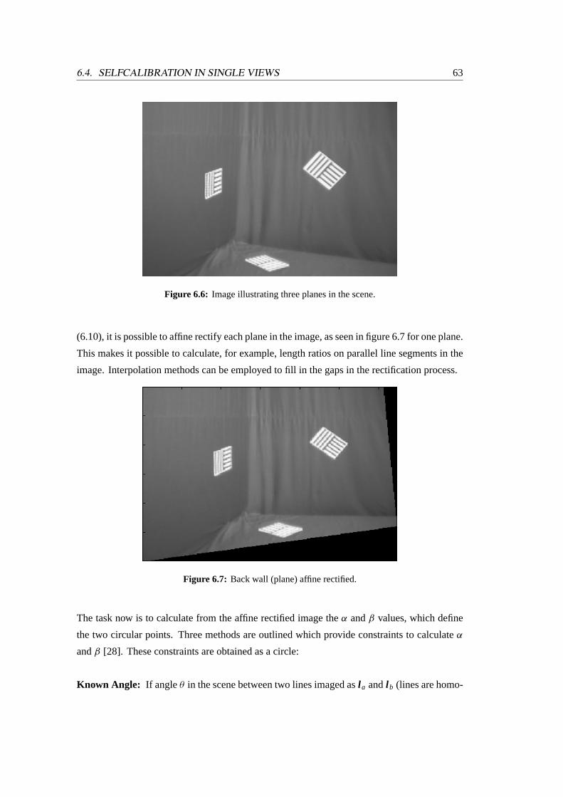
6.4. SELFCALIBRATION IN SINGLE VIEWS 63
Figure 6.6: Image illustrating three planes in the scene.
(6.10), it is possible to affine rectify each plane in the image, as seen in figure 6.7 for one plane.
This makes it possible to calculate, for example, length ratios on parallel line segments in the
image. Interpolation methods can be employed to fill in the gaps in the rectification process.
Figure 6.7: Back wall (plane) affine rectified.
The task now is to calculate from the affine rectified image theα andβ values, which define
the two circular points. Three methods are outlined which provide constraints to calculateα
andβ [28]. These constraints are obtained as a circle:
Known Angle: If angleθ in the scene between two lines imaged asl a andl b (lines are homo-
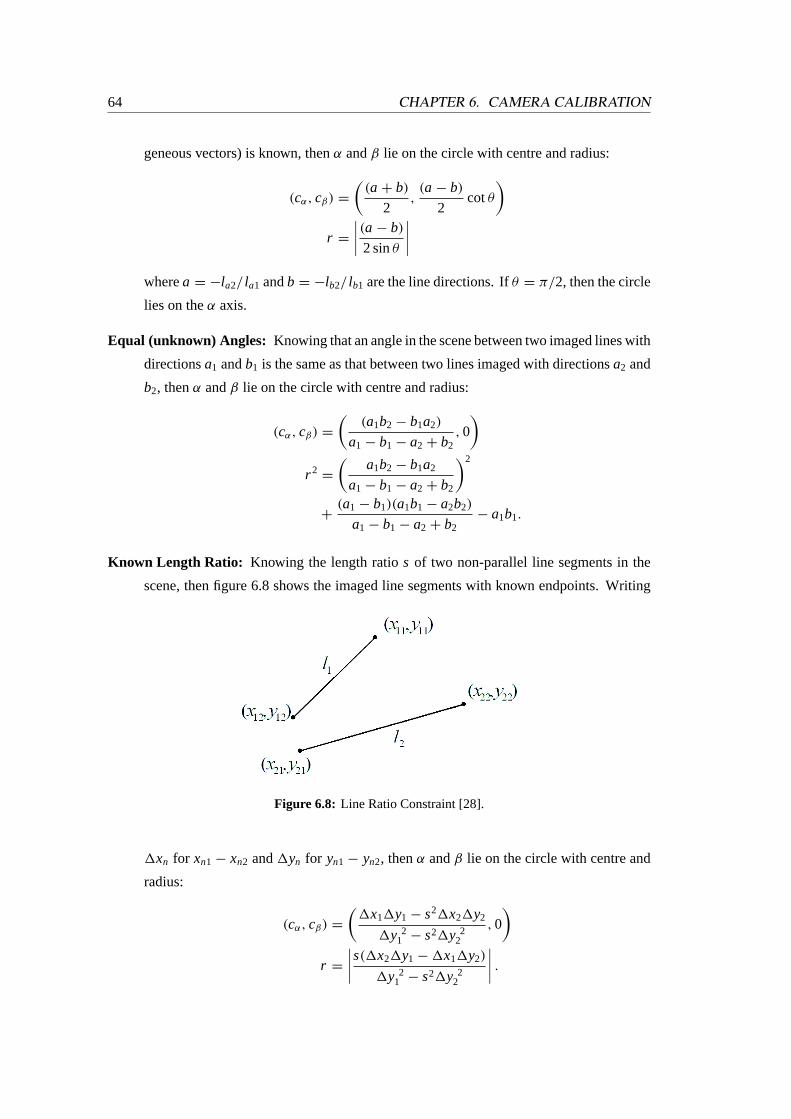
64 CHAPTER 6. CAMERA CALIBRATION
geneous vectors) is known, thenα andβ lie on the circle with centre and radius:
(cα, cβ) =
((a + b)
2,(a − b)
2cotθ
)r =
∣∣∣∣(a − b)
2 sinθ
∣∣∣∣wherea = −la2/ la1 andb = −lb2/ lb1 are the line directions. Ifθ = π/2, then the circle
lies on theα axis.
Equal (unknown) Angles: Knowing that an angle in the scene between two imaged lines with
directionsa1 andb1 is the same as that between two lines imaged with directionsa2 and
b2, thenα andβ lie on the circle with centre and radius:
(cα, cβ) =
((a1b2 − b1a2)
a1 − b1 − a2 + b2, 0
)r 2
=
(a1b2 − b1a2
a1 − b1 − a2 + b2
)2
+(a1 − b1)(a1b1 − a2b2)
a1 − b1 − a2 + b2− a1b1.
Known Length Ratio: Knowing the length ratios of two non-parallel line segments in the
scene, then figure 6.8 shows the imaged line segments with known endpoints. Writing
Figure 6.8: Line Ratio Constraint [28].
1xn for xn1 − xn2 and1yn for yn1 − yn2, thenα andβ lie on the circle with centre and
radius:
(cα, cβ) =
(1x11y1 − s21x21y2
1y 21 − s21y 2
2
, 0
)r =
∣∣∣∣s(1x21y1 − 1x11y2)
1y 21 − s21y 2
2
∣∣∣∣ .
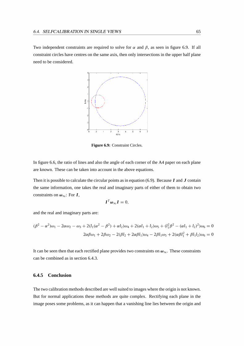
6.4. SELFCALIBRATION IN SINGLE VIEWS 65
Two independent constraints are required to solve forα andβ, as seen in figure 6.9. If all
constraint circles have centres on the same axis, then only intersections in the upper half plane
need to be considered.
Figure 6.9: Constraint Circles.
In figure 6.6, the ratio of lines and also the angle of each corner of the A4 paper on each plane
are known. These can be taken into account in the above equations.
Then it is possible to calculate the circular points as in equation (6.9). BecauseI andJ contain
the same information, one takes the real and imaginary parts of either of them to obtain two
constraints onω∞: For I ,
I Tω∞ I = 0,
and the real and imaginary parts are:
(β2− α2)ω1 − 2αω2 − ω3 + 2(l1(α
2− β2) + αl2)ω4 + 2(αl1 + l2)ω5 + (l 2
1β2− (αl1 + l2)
2)ω6 = 0
2αβω1 + 2βω2 − 2(βl2 + 2αβl1)ω4 − 2βl1ω5 + 2(αβl 21 + βl1l2)ω6 = 0
It can be seen then that each rectified plane provides two constraints onω∞. These constraints
can be combined as in section 6.4.3.
6.4.5 Conclusion
The two calibration methods described are well suited to images where the origin is not known.
But for normal applications these methods are quite complex. Rectifying each plane in the
image poses some problems, as it can happen that a vanishing line lies between the origin and
66 CHAPTER 6. CAMERA CALIBRATION
the plane to be rectified, and this will warp points closest to the vanishing line to infinity. To
compensate for this, the image needs to be translated before rectification.
The rectification process also sometimes creates very large images, which are difficult to work
with.
The whole calibration process is also difficult to automate, as the user generally has to select the
correct parallel lines or select some features on each plane to obtain the necessary constraints.
6.5 Calibration using a Planar Pattern
6.5.1 Introduction
This section describes an implementation of the camera calibration toolbox similar to that
developed by Bouguet1. He bases his calibration technique on papers by Zhang [51, 53] and
the internal camera model on a paper by Heikkilä and Silvén [22]. In the implementation
presented, however, the internal camera model is entirely based on Zhang’s technique [51, 53],
which is identical to the camera calibration matrix of equation (3.4).
6.5.2 Homography between the Planar Object and its Image
Figure 6.10 shows a square planar calibration pattern consisting of 7× 7 blocks of known
length of 25mm.
To establish the homography between the planar object and its image, it can be assumed that
the planar object lies atZ = 0 in the world coordinate system. Making use of equations (3.1)
and (3.8), and representing thei th column vector of the rotation matrixR by r i , the following
1The Camera Calibration Toolbox forMatlabr by Jean-Yves Bouguet can be downloaded from his homepageat Caltech: http : //www.vision.caltech.edu/bouguet j/calib_doc/ index.html (accessed November 2000).The C implementation of this toolbox is included in the freeOpen Source Computer Vision Library(©2000 IntelCorporation) at http://www.intel.com/research/mrl/research/cvlib/ (accessed November 2000).
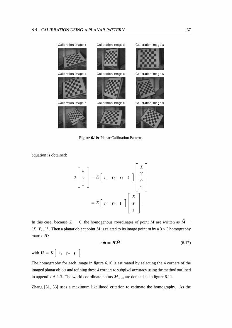
6.5. CALIBRATION USING A PLANAR PATTERN 67
Figure 6.10: Planar Calibration Patterns.
equation is obtained:
s
u
v
1
= K[
r 1 r 2 r 3 t]
X
Y
0
1
= K[
r 1 r 2 t]
X
Y
1
.
In this case, becauseZ = 0, the homogenous coordinates of pointM are written asM =
[X, Y, 1]T . Then a planar object pointM is related to its image pointm by a 3×3 homography
matrix H :
sm = H M , (6.17)
with H = K[
r 1 r 2 t].
The homography for each image in figure 6.10 is estimated by selecting the 4 corners of the
imaged planar object and refining these 4 corners to subpixel accuracy using the method outlined
in appendix A.1.3. The world coordinate pointsM 1...4 are defined as in figure 6.11.
Zhang [51, 53] uses a maximum likelihood criterion to estimate the homography. As the
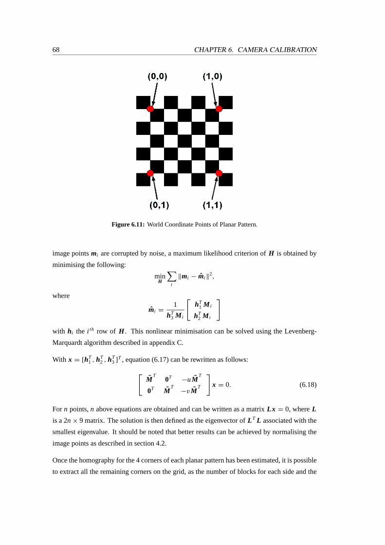
68 CHAPTER 6. CAMERA CALIBRATION
Figure 6.11: World Coordinate Points of Planar Pattern.
image pointsmi are corrupted by noise, a maximum likelihood criterion ofH is obtained by
minimising the following:
minH
∑i
‖mi − mi ‖2,
where
mi =1
hT3 M i
[hT
1 M i
hT2 M i
]
with hi the i th row of H . This nonlinear minimisation can be solved using the Levenberg-
Marquardt algorithm described in appendix C.
With x = [hT1 , hT
2 , hT3 ]
T , equation (6.17) can be rewritten as follows:[M
T0T
−uMT
0T MT
−vMT
]x = 0. (6.18)
For n points,n above equations are obtained and can be written as a matrixLx = 0, whereL
is a 2n × 9 matrix. The solution is then defined as the eigenvector ofL T L associated with the
smallest eigenvalue. It should be noted that better results can be achieved by normalising the
image points as described in section 4.2.
Once the homography for the 4 corners of each planar pattern has been estimated, it is possible
to extract all the remaining corners on the grid, as the number of blocks for each side and the
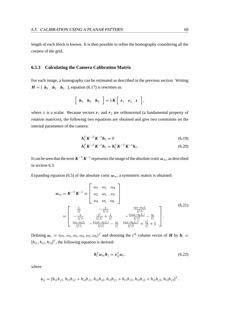
6.5. CALIBRATION USING A PLANAR PATTERN 69
length of each block is known. It is then possible to refine the homography considering all the
corners of the grid.
6.5.3 Calculating the Camera Calibration Matrix
For each image, a homography can be estimated as described in the previous section. Writing
H = [ h1 h2 h3 ], equation (6.17) is rewritten as:
[h1 h2 h3
]= λK
[r 1 r 2 t
],
whereλ is a scalar. Because vectorsr 1 and r 2 are orthonormal (a fundamental property of
rotation matrices), the following two equations are obtained and give two constraints on the
internal parameters of the camera:
hT1 K−T K−1h2 = 0 (6.19)
hT1 K−T K−1h1 = hT
2 K−T K−1h2. (6.20)
It can be seen that the termK−T K−1 represents the image of the absolute conicω∞, as described
in section 6.3.
Expanding equation (6.5) of the absolute conicω∞, a symmetric matrix is obtained:
ω∞ = K−T K−1≡
ω1 ω2 ω4
ω2 ω3 ω5
ω4 ω5 ω6
=
1f 2u
−s
f 2u fv
v0s−u0 fvf 2u fv
−s
f 2u fv
s2
f 2u f 2
v+
1f 2v
−s(v0s−u0 fv)
f 2u f 2
v−
v0f 2v
v0s−u0 fvf 2u fv
−s(v0s−u0 fv)
f 2u f 2
v−
v0f 2v
(v0s−u0 fv)2
f 2u f 2
v+
v20
f 2v
+ 1
.
(6.21)
Defining ωv = (ω1, ω2, ω3, ω4, ω5, ω6)T and denoting thei th column vector ofH by hi =
[hi 1, hi 2, hi 3]T , the following equation is derived:
hTi ω∞h j = vT
i j ωv, (6.22)
where
vi j = [hi 1h j 1, hi 1h j 2 + hi 2h j 1, hi 2h j 2, hi 3h j 1 + hi 1h j 3, hi 3h j 2 + hi 2h j 3, hi 3h j 3]T .
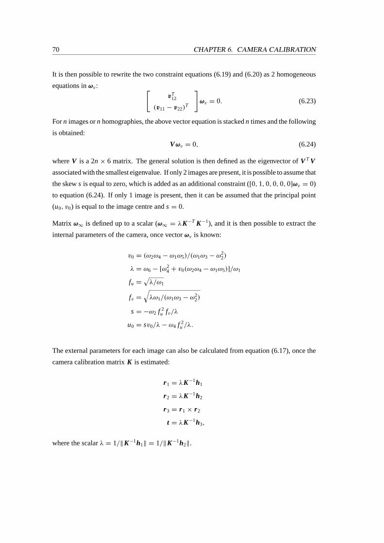
70 CHAPTER 6. CAMERA CALIBRATION
It is then possible to rewrite the two constraint equations (6.19) and (6.20) as 2 homogeneous
equations inωv: [vT
12
(v11 − v22)T
]ωv = 0. (6.23)
Forn images orn homographies, the above vector equation is stackedn times and the following
is obtained:
Vωv = 0, (6.24)
whereV is a 2n × 6 matrix. The general solution is then defined as the eigenvector ofV T V
associated with the smallest eigenvalue. If only 2 images are present, it is possible to assume that
the skews is equal to zero, which is added as an additional constraint ([0, 1, 0, 0, 0, 0]ωv = 0)
to equation (6.24). If only 1 image is present, then it can be assumed that the principal point
(u0, v0) is equal to the image centre ands = 0.
Matrix ω∞ is defined up to a scalar (ω∞ = λK−T K−1), and it is then possible to extract the
internal parameters of the camera, once vectorωv is known:
v0 = (ω2ω4 − ω1ω5)/(ω1ω3 − ω22)
λ = ω6 − [ω24 + v0(ω2ω4 − ω1ω5)]/ω1
fu =√
λ/ω1
fv =
√λω1/(ω1ω3 − ω2
2)
s = −ω2 f 2u fv/λ
u0 = sv0/λ − ω4 f 2u /λ.
The external parameters for each image can also be calculated from equation (6.17), once the
camera calibration matrixK is estimated:
r 1 = λK−1h1
r 2 = λK−1h2
r 3 = r 1 × r 2
t = λK−1h3,
where the scalarλ = 1/‖K−1h1‖ = 1/‖K−1h2‖.
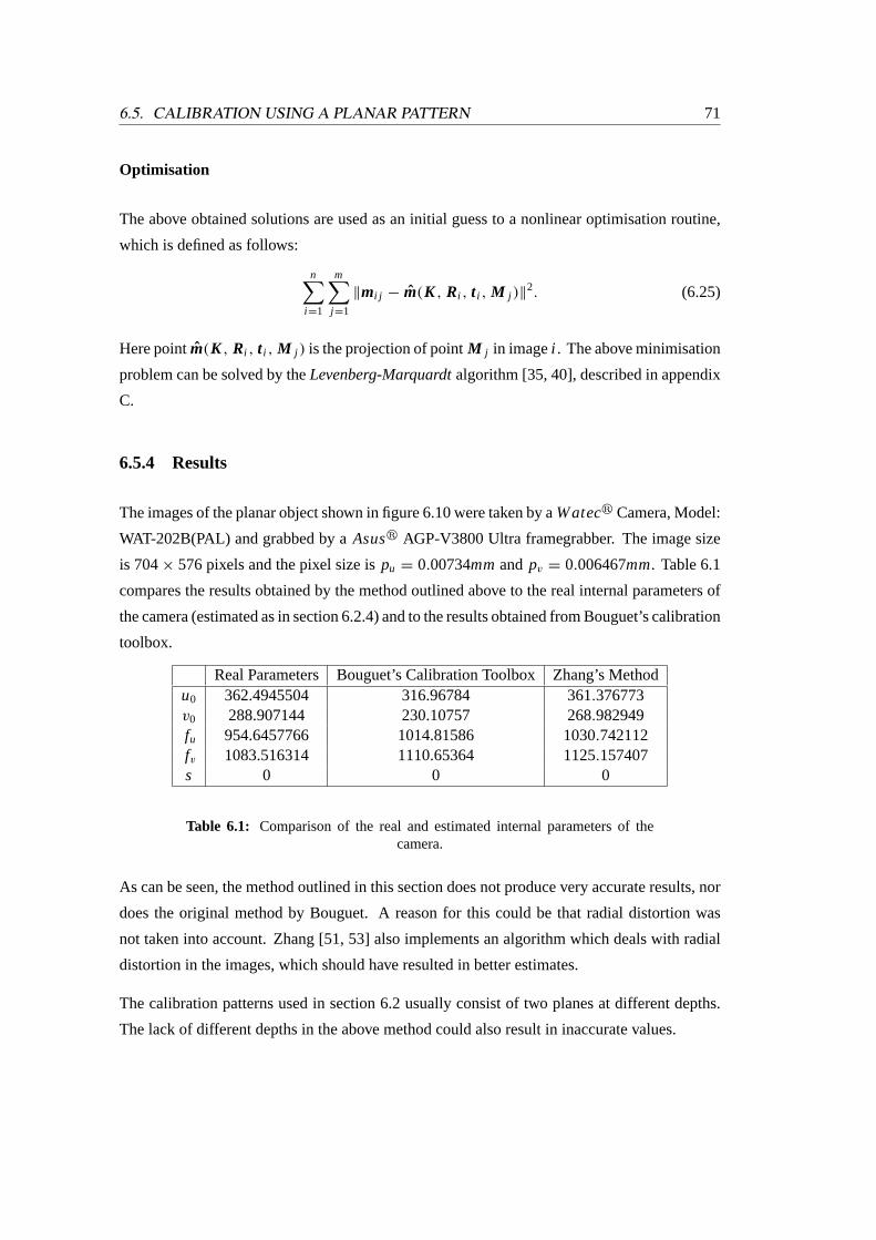
6.5. CALIBRATION USING A PLANAR PATTERN 71
Optimisation
The above obtained solutions are used as an initial guess to a nonlinear optimisation routine,
which is defined as follows:
n∑i =1
m∑j =1
‖mi j − m(K , Ri , t i , M j )‖2. (6.25)
Here pointm(K , Ri , t i , M j ) is the projection of pointM j in imagei . The above minimisation
problem can be solved by theLevenberg-Marquardtalgorithm [35, 40], described in appendix
C.
6.5.4 Results
The images of the planar object shown in figure 6.10 were taken by aWatecr Camera, Model:
WAT-202B(PAL) and grabbed by aAsusr AGP-V3800 Ultra framegrabber. The image size
is 704× 576 pixels and the pixel size ispu = 0.00734mmand pv = 0.006467mm. Table 6.1
compares the results obtained by the method outlined above to the real internal parameters of
the camera (estimated as in section 6.2.4) and to the results obtained from Bouguet’s calibration
toolbox.
Real Parameters Bouguet’s Calibration Toolbox Zhang’s Methodu0 362.4945504 316.96784 361.376773v0 288.907144 230.10757 268.982949fu 954.6457766 1014.81586 1030.742112fv 1083.516314 1110.65364 1125.157407s 0 0 0
Table 6.1: Comparison of the real and estimated internal parameters of thecamera.
As can be seen, the method outlined in this section does not produce very accurate results, nor
does the original method by Bouguet. A reason for this could be that radial distortion was
not taken into account. Zhang [51, 53] also implements an algorithm which deals with radial
distortion in the images, which should have resulted in better estimates.
The calibration patterns used in section 6.2 usually consist of two planes at different depths.
The lack of different depths in the above method could also result in inaccurate values.

72 CHAPTER 6. CAMERA CALIBRATION
Chapter 7
Stratified 3D Reconstruction
7.1 Introduction
This chapter outlines the steps involved in obtaining a 3D model of an object in a stereo image
pair. As mentioned in chapter 2, it is possible to divide 3D vision into geometry groups. This
so-called stratification is used in this chapter to calculate the geometric relationships between
structures in the image pair.
As explained later in this chapter, the reconstruction algorithm relies heavily on the parallel
lines estimated from objects in the images. In fact, it is necessary to obtain parallel lines on 3
different planes pointing in 3 different directions. As such, the model to be reconstructed has
to consist of at least 3 planes with different orientations in space, with each plane providing
attributes such as parallel markers or structures. This of course puts a great constraint on the
models which can be reconstructed. Essentially, simple geometric models such as a cube or
the corner of a room provide the necessary constraints. In order to reconstruct any arbitrary
object, it needs to be placed inside a scene providing the above mentioned constraints.
Section 7.2 explains the 3 steps of the reconstruction algorithm. Once a full 3D reconstruction
has been obtained, section 7.3 shows howdense stereo matchingis used to obtain a 3D textured
model.
73
74 CHAPTER 7. STRATIFIED 3D RECONSTRUCTION
7.2 3D Reconstruction
This section follows the structure of chapter 2 very closely. Three steps are needed to obtain a
full metric reconstruction, the first step being a projective reconstruction followed by an affine
and metric one.
7.2.1 Projective Reconstruction
For this step, the fundamental matrixF needs to be estimated from corner point matches, as
already outlined in section 4. The fundamental matrix then provides the means to compute the
two projective camera matrices for both the images.
Let the first camera coincide with the origin of the world coordinate system. The projective
camera matrix for the first camera is then defined as follows:
P1 =
[I 3×3 03
]. (7.1)
The second projective camera matrix is chosen such that the epipolar geometry corresponds to
the retrieved fundamental matrix [37, 52]. Usually it is defined as follows:
P2 =
[M σ e2
], (7.2)
wheree2 is the epipole in the second image andM is a factor of the fundamental matrix:
F = [e2]x M , where[e2]x is the antisymmetric matrix of epipolee2 as described in equation
(2.6). This epipole can be extracted from the fundamental matrix as explained in section 4.3.
Variableσ represents the global scale of the reconstruction, and as that scale is not known, it
is arbitrarily chosen and set to 1. MatrixM is defined as follows:
M = −1
‖e2‖2[e2]x F .
The matrixM is not necessarily unique, because ifM is a solution, thenM + e2vT is also a
solution for any vectorv [52].
Some reconstructions may appear distorted, and Pollefeys [37] points out that this happens
when the plane at infinity crosses the scene. He suggests estimating vectorv in such a way
that the plane at infinity does not cross the scene. Pollefeys makes use of oriented projective
geometry [26] to remedy this. The examples in this thesis did not have the problem described
and therefore vectorv = [1, 1, 1]T .
7.2. 3D RECONSTRUCTION 75
7.2.2 Affine Reconstruction
This step involves finding the plane at infinity. As mentioned in section 2.3.2, to upgrade
a specific projective representation to an affine representation, a transformation needs to be
applied which brings the plane at infinity to its canonical position. This can be achieved with
the matrixT P A defined in equation (2.27). The two affine projection matrices can then be
defined as follows [37]:
PAi = Pi T−1P A for i = 1, 2. (7.3)
The plane at infinity can be calculated if three or more points on that plane are known. These
points are points at infinity and are projections of vanishing points in space. Vanishing points are
the intersections of two or more imaged parallel lines (see appendix B). In order to determine
the three vanishing points, Faugeras et. al. [11] state that three non-coplanar directions of
parallel lines need to be established.
This can easily be verified: as figure 7.1 shows, it can happen that imaged parallel lines from
two different planes but pointing in the same direction intersect in the same vanishing point.
In the figure, the green and blue imaged parallel lines, although on different planes, intersect
in the same vanishing point.
Another problem observed is the one illustrated in figure 7.2. Although all imaged parallel lines
lie on three different planes and point in three different directions, all three vanishing point lie
on one line, as the normalised vanishing points show. A plane can only be estimated with two
or more lines, thus with only one line the plane at infinity cannot be accurately defined.
A correct estimation of the three vanishing points is shown in figure 7.3, where the normalised
vanishing points clearly illustrate that they lie on two lines which define the plane at infinity
very accurately.
Lines in the image are found with the algorithm by Burns et. al. [4] outlined in appendix
A.2. Parallel lines in three different planes and directions are selected by the user as figure 7.4
shows.
Projecting the three vanishing points into space with the two projection camera matrices of
equations (7.1) and (7.2), the points at infinity are estimated. Triangulation (see appendix D)
is employed to find the best estimate of each point in space. From the three points at infinity,
the plane at infinity is calculated as follows:
V Ti π∞ = 0 for i = 1 . . . 3, (7.4)
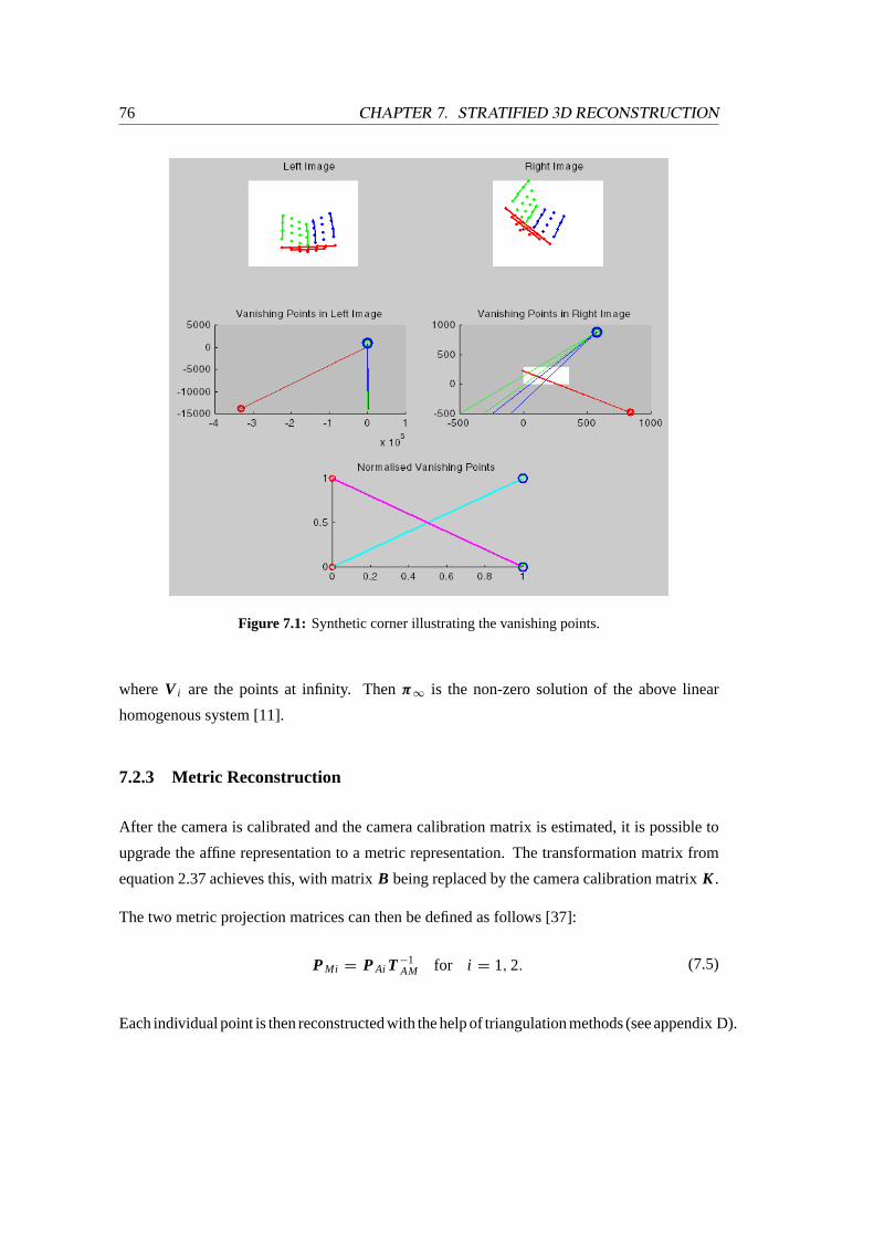
76 CHAPTER 7. STRATIFIED 3D RECONSTRUCTION
Figure 7.1: Synthetic corner illustrating the vanishing points.
whereV i are the points at infinity. Thenπ∞ is the non-zero solution of the above linear
homogenous system [11].
7.2.3 Metric Reconstruction
After the camera is calibrated and the camera calibration matrix is estimated, it is possible to
upgrade the affine representation to a metric representation. The transformation matrix from
equation 2.37 achieves this, with matrixB being replaced by the camera calibration matrixK .
The two metric projection matrices can then be defined as follows [37]:
PMi = PAi T−1AM for i = 1, 2. (7.5)
Each individual point is then reconstructed with the help of triangulation methods (see appendix D).
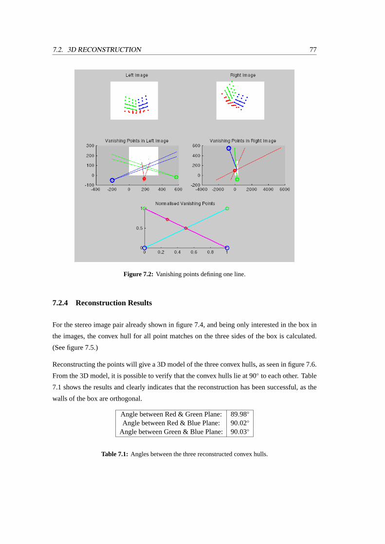
7.2. 3D RECONSTRUCTION 77
Figure 7.2: Vanishing points defining one line.
7.2.4 Reconstruction Results
For the stereo image pair already shown in figure 7.4, and being only interested in the box in
the images, the convex hull for all point matches on the three sides of the box is calculated.
(See figure 7.5.)
Reconstructing the points will give a 3D model of the three convex hulls, as seen in figure 7.6.
From the 3D model, it is possible to verify that the convex hulls lie at 90◦ to each other. Table
7.1 shows the results and clearly indicates that the reconstruction has been successful, as the
walls of the box are orthogonal.
Angle between Red & Green Plane:89.98◦
Angle between Red & Blue Plane: 90.02◦
Angle between Green & Blue Plane:90.03◦
Table 7.1: Angles between the three reconstructed convex hulls.
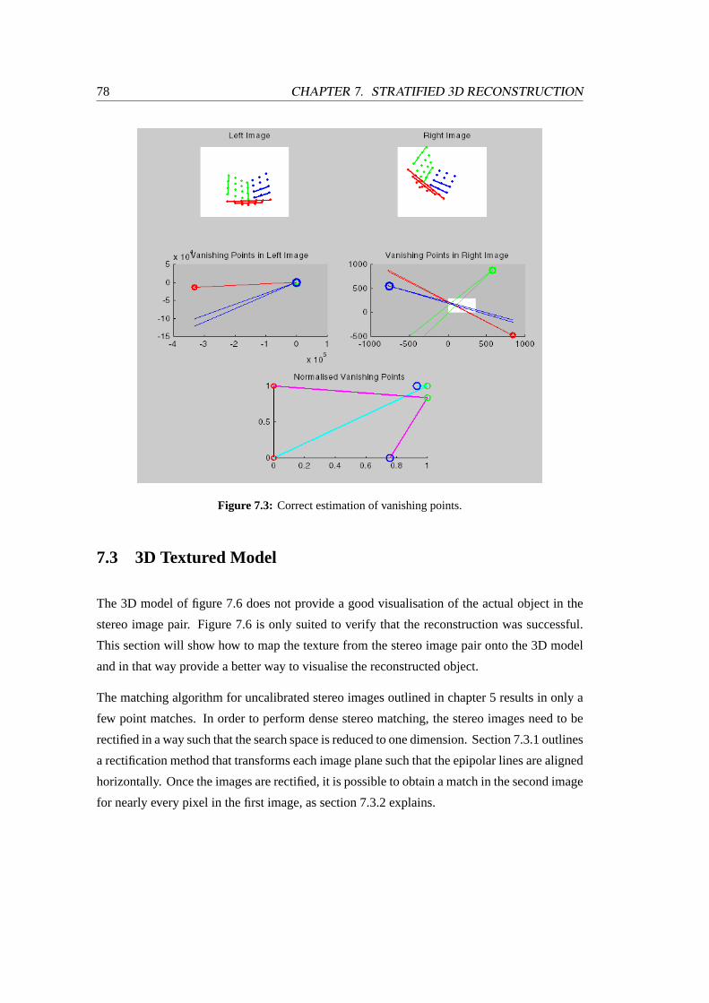
78 CHAPTER 7. STRATIFIED 3D RECONSTRUCTION
Figure 7.3: Correct estimation of vanishing points.
7.3 3D Textured Model
The 3D model of figure 7.6 does not provide a good visualisation of the actual object in the
stereo image pair. Figure 7.6 is only suited to verify that the reconstruction was successful.
This section will show how to map the texture from the stereo image pair onto the 3D model
and in that way provide a better way to visualise the reconstructed object.
The matching algorithm for uncalibrated stereo images outlined in chapter 5 results in only a
few point matches. In order to perform dense stereo matching, the stereo images need to be
rectified in a way such that the search space is reduced to one dimension. Section 7.3.1 outlines
a rectification method that transforms each image plane such that the epipolar lines are aligned
horizontally. Once the images are rectified, it is possible to obtain a match in the second image
for nearly every pixel in the first image, as section 7.3.2 explains.
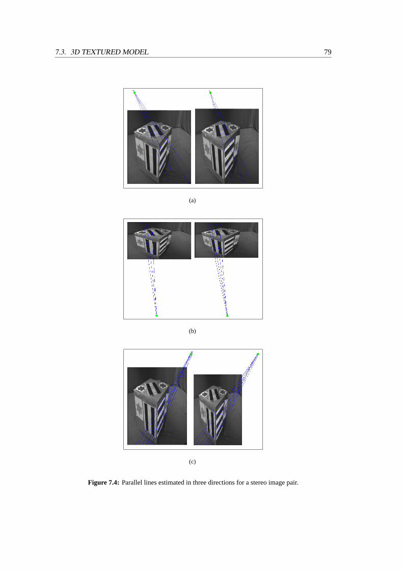
7.3. 3D TEXTURED MODEL 79
(a)
(b)
(c)
Figure 7.4: Parallel lines estimated in three directions for a stereo image pair.
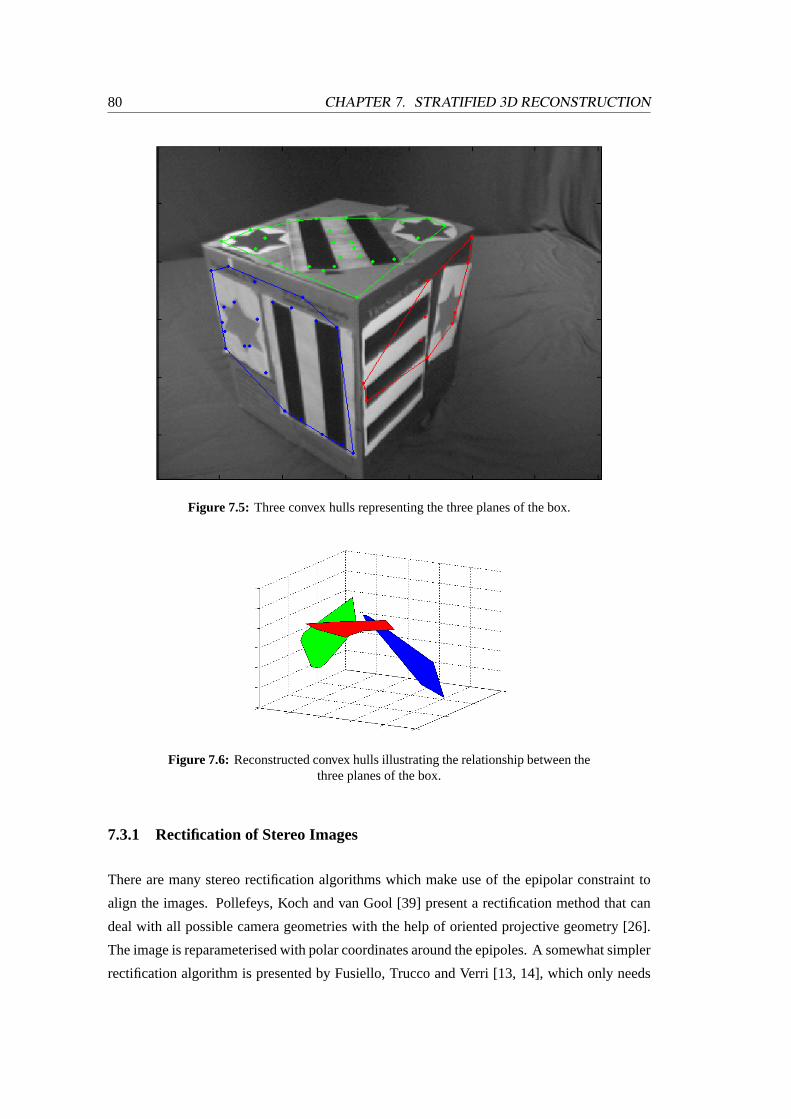
80 CHAPTER 7. STRATIFIED 3D RECONSTRUCTION
Figure 7.5: Three convex hulls representing the three planes of the box.
Figure 7.6: Reconstructed convex hulls illustrating the relationship between thethree planes of the box.
7.3.1 Rectification of Stereo Images
There are many stereo rectification algorithms which make use of the epipolar constraint to
align the images. Pollefeys, Koch and van Gool [39] present a rectification method that can
deal with all possible camera geometries with the help of oriented projective geometry [26].
The image is reparameterised with polar coordinates around the epipoles. A somewhat simpler
rectification algorithm is presented by Fusiello, Trucco and Verri [13, 14], which only needs
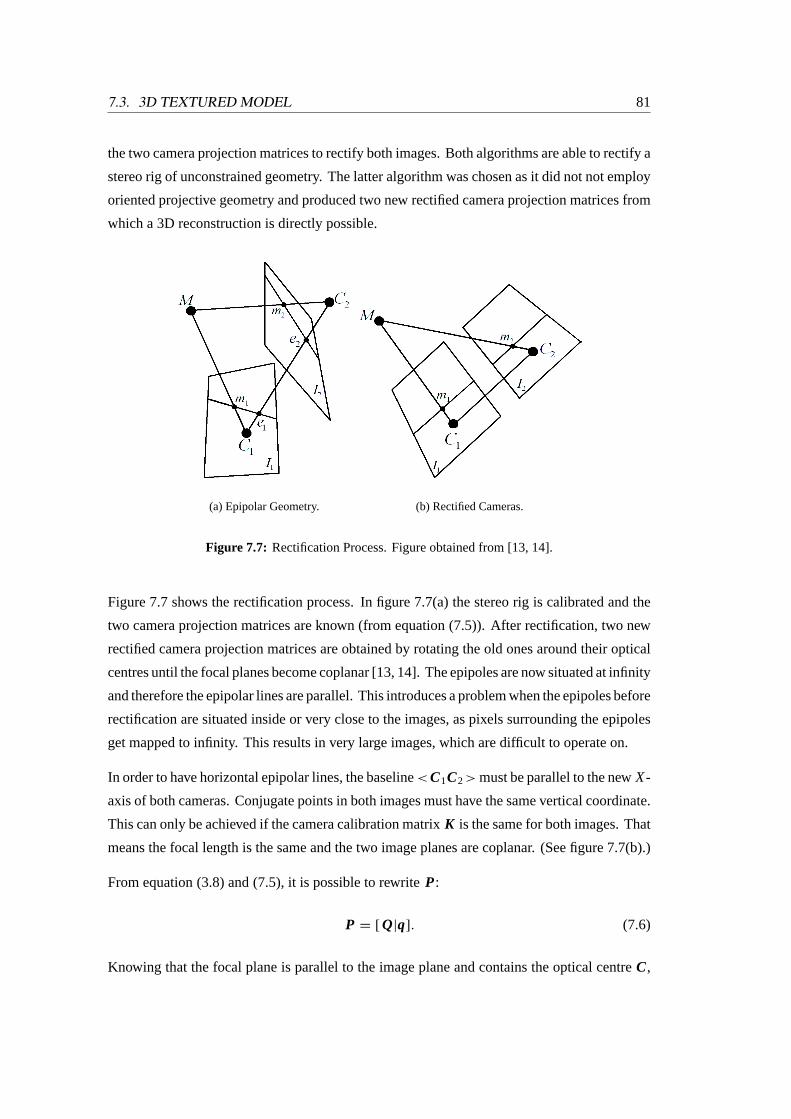
7.3. 3D TEXTURED MODEL 81
the two camera projection matrices to rectify both images. Both algorithms are able to rectify a
stereo rig of unconstrained geometry. The latter algorithm was chosen as it did not not employ
oriented projective geometry and produced two new rectified camera projection matrices from
which a 3D reconstruction is directly possible.
(a) Epipolar Geometry. (b) Rectified Cameras.
Figure 7.7: Rectification Process. Figure obtained from [13, 14].
Figure 7.7 shows the rectification process. In figure 7.7(a) the stereo rig is calibrated and the
two camera projection matrices are known (from equation (7.5)). After rectification, two new
rectified camera projection matrices are obtained by rotating the old ones around their optical
centres until the focal planes become coplanar [13, 14]. The epipoles are now situated at infinity
and therefore the epipolar lines are parallel. This introduces a problem when the epipoles before
rectification are situated inside or very close to the images, as pixels surrounding the epipoles
get mapped to infinity. This results in very large images, which are difficult to operate on.
In order to have horizontal epipolar lines, the baseline<C1C2> must be parallel to the newX-
axis of both cameras. Conjugate points in both images must have the same vertical coordinate.
This can only be achieved if the camera calibration matrixK is the same for both images. That
means the focal length is the same and the two image planes are coplanar. (See figure 7.7(b).)
From equation (3.8) and (7.5), it is possible to rewriteP:
P = [ Q|q]. (7.6)
Knowing that the focal plane is parallel to the image plane and contains the optical centreC,
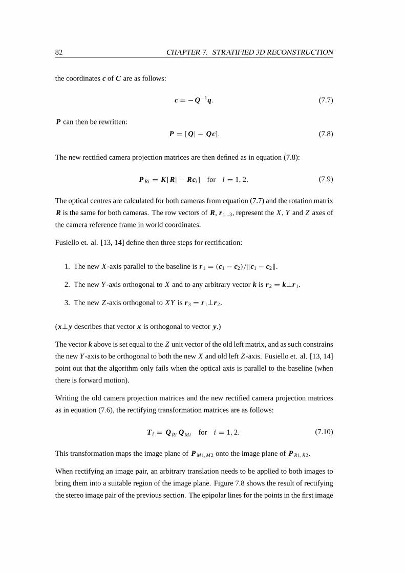
82 CHAPTER 7. STRATIFIED 3D RECONSTRUCTION
the coordinatesc of C are as follows:
c = − Q−1q. (7.7)
P can then be rewritten:
P = [ Q| − Qc]. (7.8)
The new rectified camera projection matrices are then defined as in equation (7.8):
PRi = K [R| − Rci ] for i = 1, 2. (7.9)
The optical centres are calculated for both cameras from equation (7.7) and the rotation matrix
R is the same for both cameras. The row vectors ofR, r 1...3, represent theX, Y andZ axes of
the camera reference frame in world coordinates.
Fusiello et. al. [13, 14] define then three steps for rectification:
1. The newX-axis parallel to the baseline isr 1 = (c1 − c2)/‖c1 − c2‖.
2. The newY-axis orthogonal toX and to any arbitrary vectork is r 2 = k⊥r 1.
3. The newZ-axis orthogonal toXY is r 3 = r 1⊥r 2.
(x⊥y describes that vectorx is orthogonal to vectory.)
The vectork above is set equal to theZ unit vector of the old left matrix, and as such constrains
the newY-axis to be orthogonal to both the newX and old leftZ-axis. Fusiello et. al. [13, 14]
point out that the algorithm only fails when the optical axis is parallel to the baseline (when
there is forward motion).
Writing the old camera projection matrices and the new rectified camera projection matrices
as in equation (7.6), the rectifying transformation matrices are as follows:
T i = QRi QMi for i = 1, 2. (7.10)
This transformation maps the image plane ofPM1,M2 onto the image plane ofPR1,R2.
When rectifying an image pair, an arbitrary translation needs to be applied to both images to
bring them into a suitable region of the image plane. Figure 7.8 shows the result of rectifying
the stereo image pair of the previous section. The epipolar lines for the points in the first image
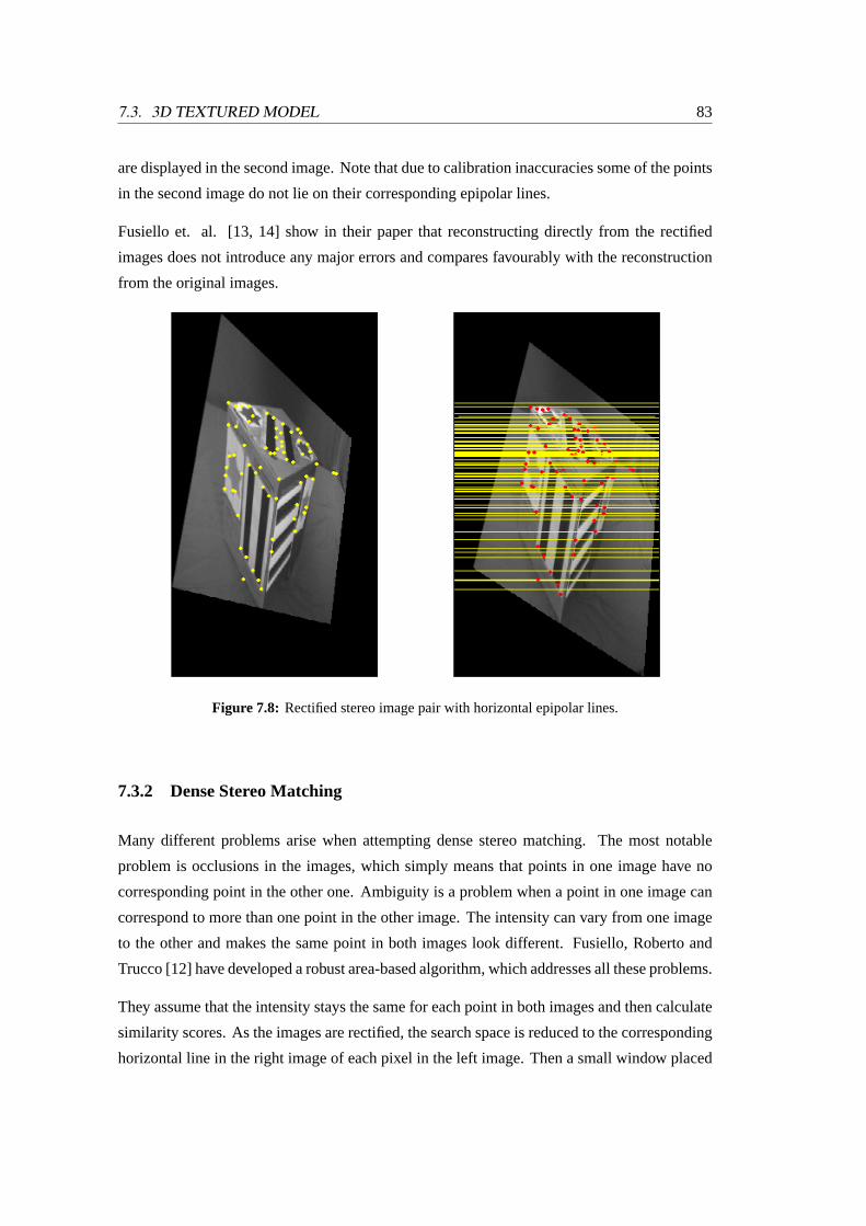
7.3. 3D TEXTURED MODEL 83
are displayed in the second image. Note that due to calibration inaccuracies some of the points
in the second image do not lie on their corresponding epipolar lines.
Fusiello et. al. [13, 14] show in their paper that reconstructing directly from the rectified
images does not introduce any major errors and compares favourably with the reconstruction
from the original images.
Figure 7.8: Rectified stereo image pair with horizontal epipolar lines.
7.3.2 Dense Stereo Matching
Many different problems arise when attempting dense stereo matching. The most notable
problem is occlusions in the images, which simply means that points in one image have no
corresponding point in the other one. Ambiguity is a problem when a point in one image can
correspond to more than one point in the other image. The intensity can vary from one image
to the other and makes the same point in both images look different. Fusiello, Roberto and
Trucco [12] have developed a robust area-based algorithm, which addresses all these problems.
They assume that the intensity stays the same for each point in both images and then calculate
similarity scores. As the images are rectified, the search space is reduced to the corresponding
horizontal line in the right image of each pixel in the left image. Then a small window placed
84 CHAPTER 7. STRATIFIED 3D RECONSTRUCTION
on each pixel in the left image is compared to a window placed in the right image along the
corresponding horizontal line. The similarity measure employed is the normalisedsum of
squared differencesor SSD error:
C(x, y, d) =
n∑i =−n
m∑j =−m
[I l (x + i, y + j ) − Ir (x + i + d, y + j )]2
√n∑
i =−n
m∑j =−m
I l (x + i, y + j )2n∑
i =−n
m∑j =−m
Ir (x + i + d, y + j )2
. (7.11)
To obtain the disparity for a pixel in the left image, the SSD error is minimsed:
dc(x, y) = arg mind
C(x, y, d). (7.12)
In order to obtain subpixel precision, a curve is fitted to the errors in the neighbourhood of the
minimum:
Dx,y = dc +1
2
C(x, y, dc − 1) − C(x, y, dc + 1)
C(x, y, dc − 1) − 2C(x, y, dc) + C(x, y, dc + 1). (7.13)
Multiple correlation windows are used to find the smallest SSD error. For each pixel in the
left image, the correlation is performed with nine different windows, as figure 7.9 shows. The
disparity with the smallest SSD error value is retained. As Fusiello et. al. [12] point out, a
window yielding a smaller SSD error is more likely to cover a constant depth region.
Figure 7.9: Nine different correlation windows. The pixel for which disparityis computed is highlighted. Figure obtained from [12].
Occlusions are detected by reversing the images and then rerunning the algorithm. This process
is calledleft-right consistency. For each point in the left image the disparitydl (x) is computed.
Then the images are reversed and the algorithm is rerun. Ifdl (x) = −dr (x + dl (x)), then
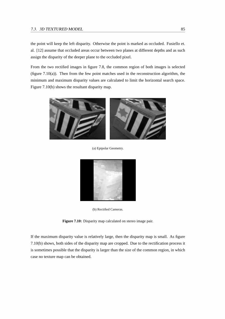
7.3. 3D TEXTURED MODEL 85
the point will keep the left disparity. Otherwise the point is marked as occluded. Fusiello et.
al. [12] assume that occluded areas occur between two planes at different depths and as such
assign the disparity of the deeper plane to the occluded pixel.
From the two rectified images in figure 7.8, the common region of both images is selected
(figure 7.10(a)). Then from the few point matches used in the reconstruction algorithm, the
minimum and maximum disparity values are calculated to limit the horizontal search space.
Figure 7.10(b) shows the resultant disparity map.
(a) Epipolar Geometry.
(b) Rectified Cameras.
Figure 7.10: Disparity map calculated on stereo image pair.
If the maximum disparity value is relatively large, then the disparity map is small. As figure
7.10(b) shows, both sides of the disparity map are cropped. Due to the rectification process it
is sometimes possible that the disparity is larger than the size of the common region, in which
case no texture map can be obtained.
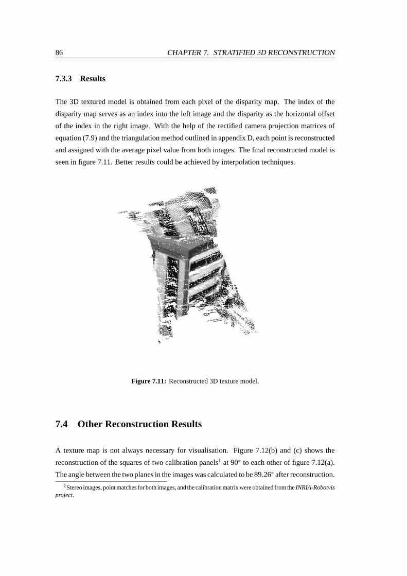
86 CHAPTER 7. STRATIFIED 3D RECONSTRUCTION
7.3.3 Results
The 3D textured model is obtained from each pixel of the disparity map. The index of the
disparity map serves as an index into the left image and the disparity as the horizontal offset
of the index in the right image. With the help of the rectified camera projection matrices of
equation (7.9) and the triangulation method outlined in appendix D, each point is reconstructed
and assigned with the average pixel value from both images. The final reconstructed model is
seen in figure 7.11. Better results could be achieved by interpolation techniques.
Figure 7.11: Reconstructed 3D texture model.
7.4 Other Reconstruction Results
A texture map is not always necessary for visualisation. Figure 7.12(b) and (c) shows the
reconstruction of the squares of two calibration panels1 at 90◦ to each other of figure 7.12(a).
The angle between the two planes in the images was calculated to be 89.26◦ after reconstruction.1Stereo images, point matches for both images, and the calibration matrix were obtained from theINRIA-Robotvis
project.
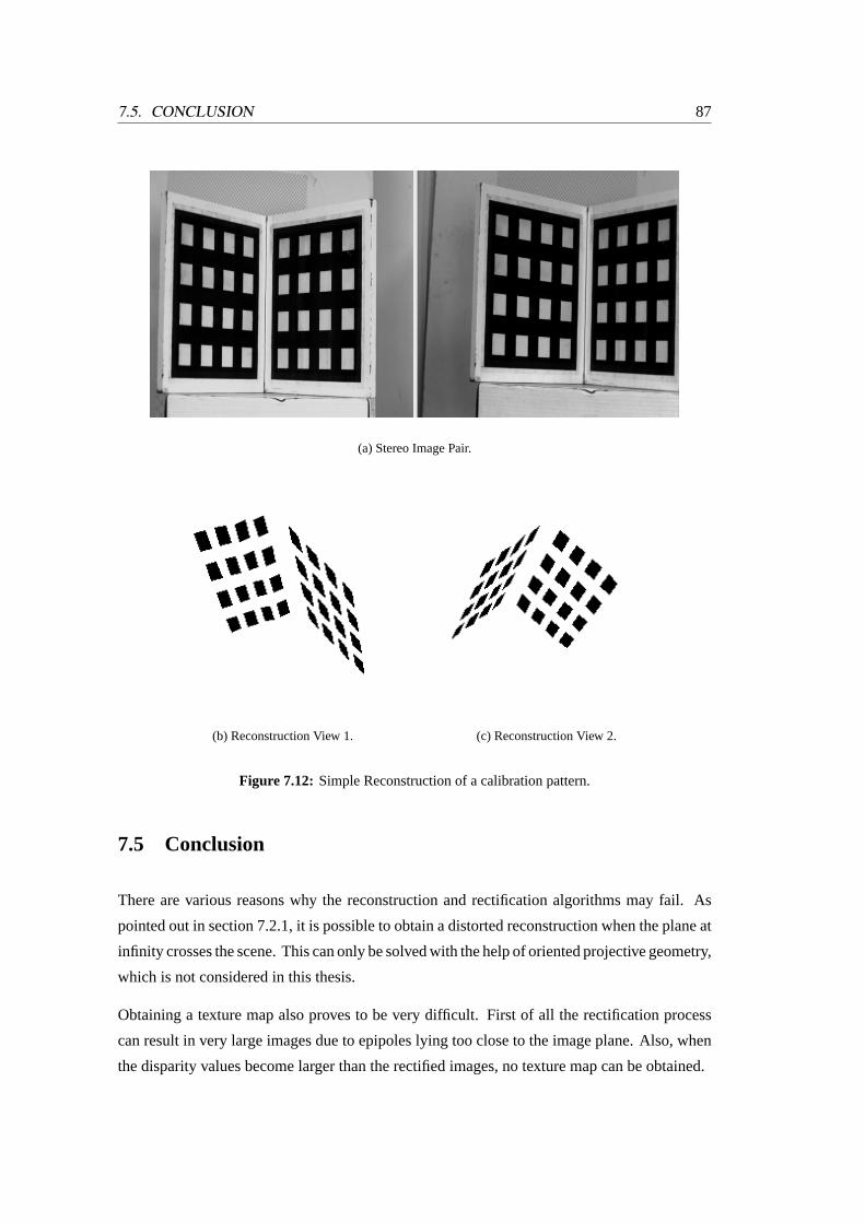
7.5. CONCLUSION 87
(a) Stereo Image Pair.
(b) Reconstruction View 1. (c) Reconstruction View 2.
Figure 7.12: Simple Reconstruction of a calibration pattern.
7.5 Conclusion
There are various reasons why the reconstruction and rectification algorithms may fail. As
pointed out in section 7.2.1, it is possible to obtain a distorted reconstruction when the plane at
infinity crosses the scene. This can only be solved with the help of oriented projective geometry,
which is not considered in this thesis.
Obtaining a texture map also proves to be very difficult. First of all the rectification process
can result in very large images due to epipoles lying too close to the image plane. Also, when
the disparity values become larger than the rectified images, no texture map can be obtained.

88 CHAPTER 7. STRATIFIED 3D RECONSTRUCTION
All those reasons made it difficult to obtain more reconstructions. The following chapter will
look at ways of solving the above problems.
Chapter 8
Conclusions
The work presented in this thesis deals with the extraction of 3D geometry from stereo images.
The problem is decomposed into a number of tasks, each task being associated with a specific
geometric group. Existing techniques have been implemented and combined to form a relatively
easy algorithm, which is straightforward to use. Minimal user intervention is achieved by
automating most of the tasks.
The matching algorithm incorporates the best aspects from two papers. The number of correct
initial matches has been improved and the algorithm is also capable of working only on a
few features. A disadvantage is the memory intensive evaluation of the correlation-weighted
proximity matrix if a few hundred features are detected in the images. A minimum of only
eight correspondences are needed for the fundamental matrix estimation, thus only the most
prominent corners should be extracted from the images. But with computing power increasing
rapidly and the cost of memory decreasing, the matching algorithm can easily operate on a
500× 500 proximity matrix.
The only part of the reconstruction algorithm which is not automated is the selection of the
imaged parallel lines in both images. It is possible to automatically select parallel lines by
detecting dominant line directions in histograms. But it is not possible to distinguish between
lines pointing in the same direction and lying on the same plane and lines pointing in the same
direction but lying on different planes. The only way to solve this is by making sure that parallel
lines in the scenes on different planes point in different directions.
The rectification algorithm implemented in this thesis works very well when the epipoles lie
far away from the images. It is impossible to make use of this algorithm if the epipoles lie
inside the images, as very large images are obtained. The rectification algorithm by Pollefeys,
89
90 CHAPTER 8. CONCLUSIONS
Koch and van Gool [39] should rather be implemented as the rectified images will always be
of a certain manageable size.
The problem with the dense stereo matching algorithm implemented in this thesis is that much of
the information on both sides of the rectified images is lost due to large calculated initial disparity
values. The only way to obtain a full textured model of the whole scene is by expanding the
stereo pair to a image sequence of the same scene. This would not only expand the possibilities
of the dense stereo matching algorithm, but it would also enable other algorithms such as the
modulus constraint[37] to be included in the reconstruction problem. It would be possible to
estimate the plane at infinity without having to define parallel lines in the scene.
Camera calibration could also be included directly in the reconstruction problem by estimating
Kruppa’s equations, instead of calibrating the camera separately. This would allow for a
system that is totally independent of any user intervention. Another interesting aspect would
be that cameras could be changed during a reconstruction task and recalibrate themselves again
automatically. But as pointed out in section 6.3.2, much work still needs to be done in that area
as the whole process of solving forKruppa’s equationsis very complex and computationally
expensive.
An advantage of breaking up the reconstruction problem into different tasks is that it makes
it possible to exchange algorithms for each part at a later stage. This is especially important
when developing this system further, without having to redefine a new approach.
A limitation of this thesis is that only rigid scenes can be considered in the reconstruction.
Moving objects in a scene would cause the reconstruction algorithm to fail. Possibly most of
the research in computer vision will be geared towards this area. An important application
must surely be the tracking of people inside a scene and obtaining a 3D model at the same time.
Appendix A
Feature Extraction
A.1 Corner Detection
A definition of a corner is "features formed at boundaries between only two image brightness
regions, where the boundary curvature is sufficiently high" [45]. One way of finding corners
in an image is by first segmenting the image in some way to find the shape of an object and
then using an edge detector to find the edge chains. Searching the edges for turnings in the
boundary will result in a corner. An example of this would be using theHough transformto
find straight lines in an image and then finding the end points of these lines. The problem
with these techniques is that they rely on prior segmentation of the shapes in the images and
inaccuracies will appear due to the segmentation. It is therefore important to find a corner
detector that operates on the image directly.
The two corner detection algorithms described here are theKitchen and Rosenfeld[23] and
Harris-Plessey[16] corner detectors. The latter one can also be used to refine the corners up
to subpixel accuracy.
A.1.1 Kitchen and Rosenfeld Corner Detector
TheKitchen and Rosenfeldcorner finder [23] is used to extract initial corners from the image
only up to pixel accuracy. This algorithm applies an edge detector to the gray level image and
finds changes in direction along the edges. These changes should correspond to turns in the
boundary of an object. This can be achieved by finding the gradient direction in the image,
91
92 APPENDIX A. FEATURE EXTRACTION
which is given by
tan(θ(x, y)) =I y(x, y)
Ix(x, y), (A.1)
whereIx andI y are the first partial derivatives of the imageI at point(x, y). The derivatives can
be calculated using horizontal and verticalSobeloperators to measure thex andy components
of the gradient in the image. TheSobeloperator is then applied to the gradient direction image
to find the changes in direction of the edge. This is the curvature measure, which is multiplied
by the gradient magnitude from the first image to obtain the corner magnitude measure.
Calculating the partial derivatives ofθ (here the arguments of functions are omitted for clarity):
θx =IxyIx − Ixx I y
I 2x + I 2
y
θy =I yyIx − IxyI y
I 2x + I 2
y
,
the corner magnitude is defined as follows:
κ =Ixθy − I yθx
I 2x + I 2
y
=Ixx I 2
y + I yyI 2x − 2IxyIx I y
I 2x + I 2
y
.
This expression finds the rate of change of gradient direction along the edge in the image,
multiplied by the gradient magnitude. It can be regarded as the curvature of a contour line.
Thresholding this image will result in points with high curvature being selected. The corners
lie along the strongest edges of the image.
A.1.2 Harris-Plessey Corner Detector
The Harris or Plesseycorner finder [16] also finds corners by considering points of high
curvature. It is based on theMoraveccorner detector [34].
The Moravec corner detector starts by looking for a large variation in intensity in some local
window in the image in every direction. This can be expressed mathematically by an autocor-
relation function, which, when thresholded, yields the desired corner points. The result was
found to be very noisy due to the rectangular nature of the window, and that the operator is very
sensitive to strong edges. Harris and Stephens [16] modified the Moravec operator by using a
circular Gaussian window.
A.1. CORNER DETECTION 93
Their autocorrelation function is as follows:
E(x, y) = Ax2+ 2Bxy+ Cy2, (A.2)
where
A = I 2x ⊗ w
B = Ixy ⊗ w
C = I 2y ⊗ w,
w = e−(winx2+winy2)/2σ2
is the smooth Gaussian window and⊗ is the convolution operator.
Variables winx and winy define the window size. The autocorrelation function can be rewritten
for small shifts:
E(x, y) = [x, y]G[x, y]T , (A.3)
where
G =
[A B
B C
](A.4)
is a 2× 2 matrix. The following operator is then used to extract corners from the image:
R(x, y) = det(G) − k (trace(G))2. (A.5)
The value fork is usually taken to be 0.04 to take into account high contrast pixel step edges
[54]. ThresholdingR will then give the desired corners.
A.1.3 Subpixel Corner Detection
To refine the corners estimated by theKitchen and RosenfeldorHarris-Plesseycorner detectors
to subpixel accuracy, an algorithm is implemented which was developed by Jean-Yves Bouguet
and included in theOpen Source Computer Vision Library(©2000 Intel Corporation)1 [6]. With
reference to figure A.1, it can be observed that every vector from the centreq to a point p in
the neighbourhood ofq is orthogonal to the image gradient atp and subject to image and
measurement noise. Pointq is the subpixel accurate corner location or sometimes also called
theradial saddle point.1The Open Source Computer Vision Library(©2000 Intel Corporation) can be downloaded from the official
website: http://www.intel.com/research/mrl/research/cvlib/ (accessed November 2000).
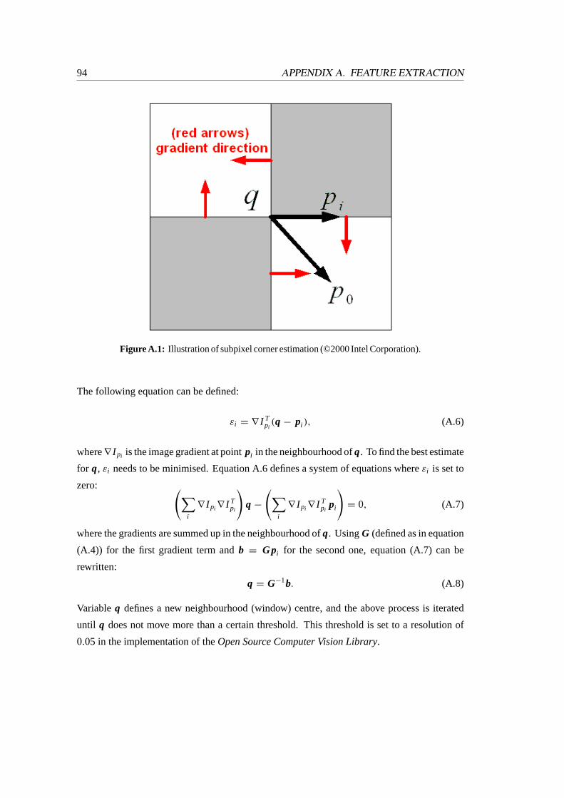
94 APPENDIX A. FEATURE EXTRACTION
Figure A.1: Illustration of subpixel corner estimation (©2000 Intel Corporation).
The following equation can be defined:
εi = ∇ I Tpi(q − pi ), (A.6)
where∇ I pi is the image gradient at pointpi in the neighbourhood ofq. To find the best estimate
for q, εi needs to be minimised. Equation A.6 defines a system of equations whereεi is set to
zero: (∑i
∇ I pi ∇ I Tpi
)q −
(∑i
∇ I pi ∇ I Tpi
pi
)= 0, (A.7)
where the gradients are summed up in the neighbourhood ofq. UsingG (defined as in equation
(A.4)) for the first gradient term andb = Gpi for the second one, equation (A.7) can be
rewritten:
q = G−1b. (A.8)
Variableq defines a new neighbourhood (window) centre, and the above process is iterated
until q does not move more than a certain threshold. This threshold is set to a resolution of
0.05 in the implementation of theOpen Source Computer Vision Library.
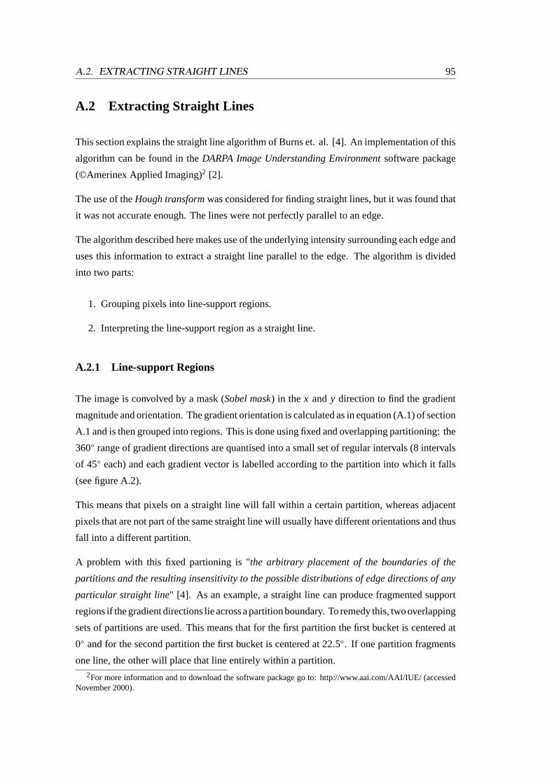
A.2. EXTRACTING STRAIGHT LINES 95
A.2 Extracting Straight Lines
This section explains the straight line algorithm of Burns et. al. [4]. An implementation of this
algorithm can be found in theDARPA Image Understanding Environmentsoftware package
(©Amerinex Applied Imaging)2 [2].
The use of theHough transformwas considered for finding straight lines, but it was found that
it was not accurate enough. The lines were not perfectly parallel to an edge.
The algorithm described here makes use of the underlying intensity surrounding each edge and
uses this information to extract a straight line parallel to the edge. The algorithm is divided
into two parts:
1. Grouping pixels into line-support regions.
2. Interpreting the line-support region as a straight line.
A.2.1 Line-support Regions
The image is convolved by a mask (Sobel mask) in the x andy direction to find the gradient
magnitude and orientation. The gradient orientation is calculated as in equation (A.1) of section
A.1 and is then grouped into regions. This is done using fixed and overlapping partitioning: the
360◦ range of gradient directions are quantised into a small set of regular intervals (8 intervals
of 45◦ each) and each gradient vector is labelled according to the partition into which it falls
(see figure A.2).
This means that pixels on a straight line will fall within a certain partition, whereas adjacent
pixels that are not part of the same straight line will usually have different orientations and thus
fall into a different partition.
A problem with this fixed partioning is "the arbitrary placement of the boundaries of the
partitions and the resulting insensitivity to the possible distributions of edge directions of any
particular straight line" [4]. As an example, a straight line can produce fragmented support
regions if the gradient directions lie across a partition boundary. To remedy this, two overlapping
sets of partitions are used. This means that for the first partition the first bucket is centered at
0◦ and for the second partition the first bucket is centered at 22.5◦. If one partition fragments
one line, the other will place that line entirely within a partition.2For more information and to download the software package go to: http://www.aai.com/AAI/IUE/ (accessed
November 2000).
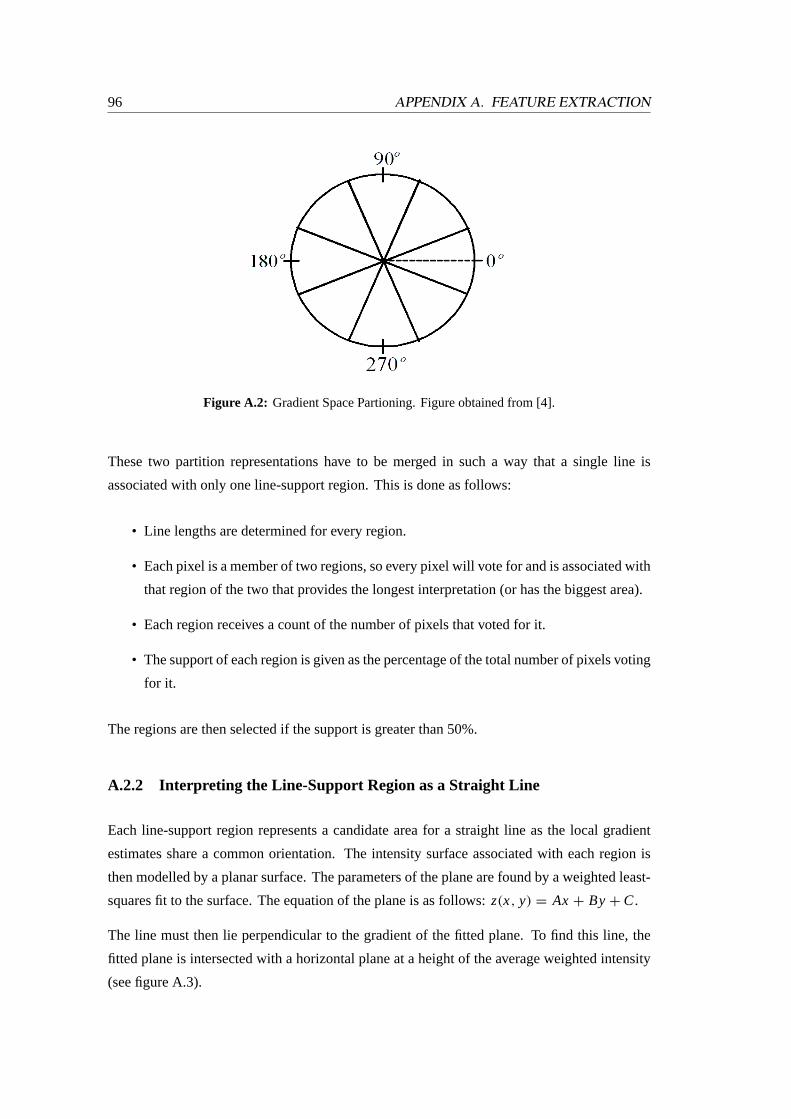
96 APPENDIX A. FEATURE EXTRACTION
Figure A.2: Gradient Space Partioning. Figure obtained from [4].
These two partition representations have to be merged in such a way that a single line is
associated with only one line-support region. This is done as follows:
• Line lengths are determined for every region.
• Each pixel is a member of two regions, so every pixel will vote for and is associated with
that region of the two that provides the longest interpretation (or has the biggest area).
• Each region receives a count of the number of pixels that voted for it.
• The support of each region is given as the percentage of the total number of pixels voting
for it.
The regions are then selected if the support is greater than 50%.
A.2.2 Interpreting the Line-Support Region as a Straight Line
Each line-support region represents a candidate area for a straight line as the local gradient
estimates share a common orientation. The intensity surface associated with each region is
then modelled by a planar surface. The parameters of the plane are found by a weighted least-
squares fit to the surface. The equation of the plane is as follows:z(x, y) = Ax + By + C.
The line must then lie perpendicular to the gradient of the fitted plane. To find this line, the
fitted plane is intersected with a horizontal plane at a height of the average weighted intensity
(see figure A.3).
A.2. EXTRACTING STRAIGHT LINES 97
Figure A.3: Two planes intersecting in a straight line. Figure obtained from [4].
The intersection is a straight line, which is parallel to the edge in the image. Once all these
lines have been found, only lines of a certain length or orientation are retained.
A comparison with the Hough transform is shown in figure A.4. The Hough transform is clearly
not as accurate as the algorithm outlined here. The reason for this is that the Hough transform
only searches for an edge and fits a line to it, while with the Burns line algorithm, the whole
area surrounding an edge is taken into account when fitting a line.
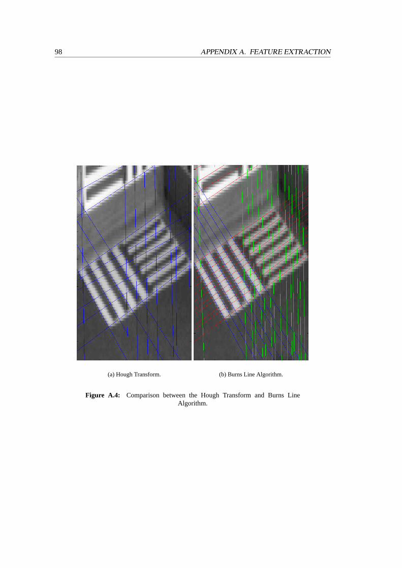
98 APPENDIX A. FEATURE EXTRACTION
(a) Hough Transform. (b) Burns Line Algorithm.
Figure A.4: Comparison between the Hough Transform and Burns LineAlgorithm.
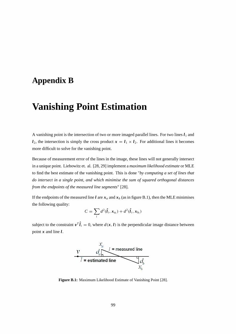
Appendix B
Vanishing Point Estimation
A vanishing point is the intersection of two or more imaged parallel lines. For two linesl 1 and
l 2, the intersection is simply the cross productx = l 1 × l 2. For additional lines it becomes
more difficult to solve for the vanishing point.
Because of measurement error of the lines in the image, these lines will not generally intersect
in a unique point. Liebowitz et. al. [28, 29] implement amaximum likelihood estimateor MLE
to find the best estimate of the vanishing point. This is done "by computing a set of lines that
do intersect in a single point, and which minimise the sum of squared orthogonal distances
from the endpoints of the measured line segments" [28].
If the endpoints of the measured linel arexa andxb (as in figure B.1), then the MLE minimises
the following quality:
C =
∑i
d2(l i , xai ) + d2(l i , xbi )
subject to the constraintvT l i = 0, whered(x, l ) is the perpendicular image distance between
point x and linel .
Figure B.1: Maximum Likelihood Estimate of Vanishing Point [28].
99

100 APPENDIX B. VANISHING POINT ESTIMATION
An initial solution forv is obtained from the null vector of the matrix[l 1, l 2, . . . , l n] via singular
value decomposition [28].
An implementation of this algorithm can be found in theDARPA Image Understanding Envi-
ronmentsoftware package (©Amerinex Applied Imaging)1.
1For more information and to download the software package go to: http://www.aai.com/AAI/IUE/ (accessedNovember 2000).
Appendix C
The Levenberg-Marquardt Algorithm
All minimisations in this thesis have been done using theLevenberg-Marquardtalgorithm
[35, 40]. A short description of the Levenberg-Marquardt algorithm is presented by Hartley
[17] and Pollefeys [38], and is outlined here. The algorithm is based on theNewton iteration
method, which is described first.
C.1 Newton Iteration
For a vector relationy = f (x), wherex and y are vectors in different dimensions, withy
a measured value fory, a desired vectorx needs to be calculated which satisfies the above
relation. Stated differently, a vectorx needs to be calculated which satisfiesy = f (x) + ε,
for which‖ε‖ is minimal. Newton’s iteration method starts with an initial valuex0 and refines
this value under the assumption that the functionf is locally linear [17, 38].
For y = f (x0)+ ε0, the functionf is approximated atx0 by f (x0 + δ) = f (x0)+ Jδ, where
J =∂ y∂x is the linear mapping represented by the Jacobian matrix. Then settingx1 = x0 + δ,
the following relation is obtained:
y − f (x1) = y − f (x0) − Jδ = ε0 − Jδ,
where‖ε0 − Jδ‖ needs to be minimised. This minimisation can be solved forδ using linear
least-squares:
JT Jδ = JTε0.
The above equation is called thenormal equation[17, 38].
101
102 APPENDIX C. THE LEVENBERG-MARQUARDT ALGORITHM
To summarise the above procedure, the solution can be found by starting with an initial estimate
x0 and approximating the equation
x i +1 = x i + δi ,
whereδi is the solution to the normal equationsJT Jδi = JTε i . Matrix J is the Jacobian at
x i andε i = y − f (x i ). As pointed out by Hartley [17] and Pollefeys [38], it is possible that
this algorithm will converge to a local minimum value or not converge at all, as it depends a
lot on the initial estimatex0.
C.2 Levenberg-Marquardt Iteration
This method varies slightly from the Newton method. The normal equationsNδ = JT Jδ =
JTε0 are augmented toN ′δ = JTε0, whereN ′i i = (1+λ)N i i and N ′
i j = N i j for i 6= j .
The value ofλ is initialised to a very small value, usuallyλ = 10−3. If the value obtained for
δ by the augmented normal equations reduces the error, then the increment is accepted andλ
is divided by 10 before the next iteration. If the error increases,λ is multiplied by 10 and the
augmented normal equations are solved until an increment is obtained which reduces the error.
The implementation of the Levenberg-Marquardt algorithm used in this thesis is from the
MINPACK1 library andDARPA Image Understanding Environmentsoftware package (©Amer-
inex Applied Imaging)2.
1For more information and to download the MINPACK software package go to: http://www.netlib.org (accessedNovember 2000).
2For more information and to download the Image Understanding Environment software package go to:http://www.aai.com/AAI/IUE/ (accessed November 2000).
Appendix D
Triangulation
The process of triangulation is needed to find the intersection of two known rays in space. Due
to measurement noise in images and some inaccuracies in the calibration matrices, these two
rays will not generally meet in a unique point. This section outlines a linear and a nonlinear
method to accurately estimate the best possible point of intersection.
D.1 Linear Triangulation
Let the 3D coordinate in space beM = [X, Y, Z, W]T and its corresponding image coordinates
bem1,2 = [u1,2, v1,2, 1]T . Then making use of the pinhole model equation (3.1) and the camera
projection matrices relating to the two images, the following two equations can be defined:
s1[u1, v1, 1]T
= P1[X, Y, Z, W]T , (D.1)
s2[u2, v2, 1]T
= P2[X, Y, Z, W]T , (D.2)
wheres1 ands2 are two arbitrary scalars. Writing thei th row of P1 and P2 as pT1i and pT
2i
respectively, the two scalarss1 ands2 can be eliminated by knowing the following:s1 = pT13M
ands2 = pT23M . The above two equations can then be rewritten in the form:
AM = 0, (D.3)
103
104 APPENDIX D. TRIANGULATION
whereA is a 4× 4 matrix:
A =
pT
11 − u1 pT13
pT12 − v1 pT
13
pT21 − u2 pT
23
pT22 − v2 pT
23
.
The solution is then the eigenvector of the matrixAT A associated with the smallest eigenvalue.
It is also possible to assume that no point is at infinity, and thenW = 1. The set of homogeneous
equations (D.3) is then reduced to a set of four non-homogeneous equations in three unknowns
[52].
D.2 Nonlinear Triangulation
The above linear method can be used as an initial estimate for a nonlinear optimisation problem.
Zhang [52] minimises the error measured in the image plane between the observation and the
projection of the reconstructed point:
(u1 −
pT11M
pT13M
)2
+
(v1 −
pT12M
pT13M
)2
+
(u2 −
pT21M
pT23M
)2
+
(v2 −
pT22M
pT23M
)2
. (D.4)
The nonlinear minimisation is done using theLevenberg-Marquardtalgorithm [35, 40], de-
scribed in appendix C.
Hartley and Sturm [21] define a different minimisation problem. Their method seeks a pair of
points that minimises the sum of squared distances subject to the epipolar constraint. But as
Zhang [52] points out in his paper, both the linear and nonlinear triangulation methods outlined
above will give optimum results.
Bibliography
[1] M.N. Armstrong. Self-Calibration from Image Sequences. PhD thesis, Department of
Engineering Science, University of Oxford, 1996.
[2] J.R. Beveridge, C. Graves, and C. Lesher. Some Lessons Learned from Coding the Burns
Line Extraction Algorithm in the DARPA Image Understanding Environment. Technical
Report CS-96-125, Computer Science Department, Colorado State University, October
1996.
[3] S. Birchfield. An Introduction to Projective Geometry (for Computer Vision). Stanford
University, March 1998.
[4] J.B. Burns, A.R. Hanson, and E.M. Riseman. Extracting Straight Lines.IEEE Transac-
tions on Pattern Analysis and Machine Intelligence, 8(4):425–455, July 1986.
[5] B. Caprile and V. Torre. Using Vanishing Points for Camera Calibration.International
Journal of Computer Vision, 4:127–140, 1990.
[6] Intel Corporation. Open Source Computer Vision Library Manual. See official website:
http://www.intel.com/research/mrl/research/cvlib/, 2000.
[7] O. Faugeras. What can be seen in three dimensions with an uncalibrated stereo rig?Com-
puter Vision-ECCV’92, Springer Verlag, Lecture Notes in Computer Science, 588:563–
578, 1992.
[8] O. Faugeras.Three-Dimensional Computer Vision: A Geometric Viewpoint. MIT Press,
1993.
[9] O. Faugeras. Stratification of 3-D vision: projective, affine, and metric representations.
Journal of the Optical Society of America, 12(3):465–484, March 1995.
105
106 BIBLIOGRAPHY
[10] O. Faugeras, Q.-T. Luong, and S. Maybank. Camera Self-Calibration: Theory and Ex-
periments. InComputer-Vision-ECCV’92, Lecture Notes in Computer Science, volume
588, pages 321–334. Springer-Verlag, 1992.
[11] O. Faugeras, L. Robert, S. Laveau, G. Csurka, C. Zeller, C. Gauclin, and I. Zoghlami.
3-D Reconstruction of Urban Scenes from Image Sequences.Computer Vision and Image
Understanding, 69(3):292–309, March 1998. Also Research Report No.2572, INRIA
Sophia-Antipolis.
[12] A. Fusiello, V. Roberto, and E. Trucco. Efficient stereo with multiple windowing. In
Proceedings of the IEEE Conference on Computer Vision and Pattern Recognition, pages
858–863, June 1997.
[13] A. Fusiello, E. Trucco, and A. Verri. Rectification with unconstrained stereo geometry.
In A.F. Clark, editor,Proceedings of the British Machine Vision Conference, pages 400–
409. BMVA Press, September 1997. Also Research Memorandum RM/98/12, 1998,
Department of Computing and Electrical Engineering, Heriot-Watt University, Edinburgh,
UK.
[14] A. Fusiello, E. Trucco, and A. Verri. A compact algorithm for rectification of stereo pairs.
Machine Vision and Applications, 12(1):16–22, 2000.
[15] G.H. Golup and C.F. van Loan.Matrix Computations. John Hopkins University Press,
2nd edition, 1996.
[16] C. Harris and M. Stephens. A Combined Corner and Edge Detector.Proceedings Alvey
Vision Conference, pages 189–192, 1988.
[17] R. Hartley. Euclidean Reconstruction from Uncalibrated Views. In J.L. Mundy, A. Zis-
serman, and D. Forsyth, editors,Applications of Invariance in Computer Vision, volume
825 ofLecture Notes in Computer Science, pages 237–256. Springer-Verlag, 1994.
[18] R. Hartley. In defense of the 8-point algorithm.IEEE Transactions on Pattern Analysis
and Machine Intelligence, 19(6):580–593, June 1997.
[19] R. Hartley. Kruppa’s Equations Derived from the Fundamental Matrix.IEEE Transactions
on Pattern Analysis and Machine Intelligence, 19(2):133–135, February 1997.
[20] R. Hartley and J.L. Mundy. The relationship between photogrammetry and computer
vision. In E.B. Barrett and D.M. McKeown, editors,SPIE Proceedings, volume 1944 of
Integrating Photogrammetric Techniques with Scene Analysis and Machine Vision, pages
92–105. SPIE Press, September 1993.
BIBLIOGRAPHY 107
[21] R. Hartley and P. Sturm. Triangulation.Computer Vision and Image Understanding,
68(2):146–157, 1997.
[22] J. Heikkilä and O. Silvén. A Four-step Camera Calibration Procedure with Implicit Image
Correction. InIEEE Computer Society Conference on Computer Vision and Pattern
Recognition (CVPR’97), San Juan, Puerto Rico, pages 1106–1112, 1997.
[23] L. Kitchen and A. Rosenfeld. Gray-level corner detection.Pattern Recognition Letters,
1(2):95–102, December 1982.
[24] R. Koch. Automatic Reconstruction of Buildings from Stereoscopic Image Sequences.
Proceedings of Eurographics ’93, 12(3):339–350, September 1993.
[25] R. Koch. 3-D Surface Reconstruction from Stereoscopic Image Sequences. InProc. 5th
International Conference on Computer Vision, Cambridge, MA., USA, pages 109–114,
June 1995.
[26] S. Laveau and O. Faugeras. Oriented Projective Geometry for Computer Vision. In
B. Buxton and R. Cipolla, editors,Computer-Vision-ECCV’96, Lecture Notes in Computer
Science, volume 1064, pages 147–156. Springer-Verlag, 1996.
[27] D. Liebowitz, A. Criminisi, and A. Zisserman. Creating Architectural Models from
Images. InProc. EuroGraphics, volume 18, pages 39–50, September 1999.
[28] D. Liebowitz and A. Zisserman. Metric Rectification for Perspective Images of Planes.
In Proceedings of the Conference on Computer Vision and Pattern Recognition, pages
482–488, 1998.
[29] D. Liebowitz and A. Zisserman. Combining Scene and Auto-calibration Constraints. In
Proc. 7th International Conference on Computer Vision, Kerkyra, Greece, pages 293–300,
September 1999.
[30] M.I.A. Lourakis and R. Deriche. Camera Self-Calibration Using the Singular Value
Decomposition of the Fundamental Matrix: From Point Correspondences to 3D Mea-
surements. Technical Report 3748, INRIA Sophia Antipolis, Project Robotvis, 1999.
[31] Q.-T. Luong and O. Faugeras. The Fundamental matrix: theory, algorithms, and stability
analysis.The International Journal of Computer Vision, 1(17):43–76, 1996.
[32] S.J. Maybank and O. Faugeras. A Theory of Self-Calibration of a Moving Camera.
International Journal of Computer Vision, 8(2):123–151, August 1992.
108 BIBLIOGRAPHY
[33] R. Mohr and B. Triggs. Projective Geometry for Image Analysis. InInternational
Symposium of Photogrammetry and Remote Sensing, Vienna, July 1996.
[34] H. Moravec. Obstacle Avoidance and Navigation in the Real World by a Seeing Robot
Rover. Technical Report CMU-RI-TR-3, Robotics Institute, Carnegie-Mellon University,
September 1980.
[35] J.J. Moré. The Levenberg-Marquardt Algorithm: Implementation and Theory. In
G.A. Watson, editor,Numerical Analysis, volume 630 ofLecture Notes in Mathemat-
ics. Springer-Verlag, 1977.
[36] M. Pilu. Uncalibrated Stereo Correspondence by Singular Value Decomposition. Tech-
nical Report HPL-97-96, Digital Media Department, HP Laboratories Bristol, August
1997.
[37] M. Pollefeys.Self-Calibration and Metric 3D Reconstruction from Uncalibrated Image
Sequences. PhD thesis, ESAT-PSI, K.U. Leuven, 1999.
[38] M. Pollefeys. Tutorial on 3D Modelling from Images. Tutorial organised in conjunction
with ECCV 2000, Dublin, Ireland, June 2000.
[39] M. Pollefeys, R. Koch, and L. van Gool. A simple and efficient rectification method for
general motion. InProc. 7th International Conference on Computer Vision, Kerkyra,
Greece, pages 496–501, September 1999.
[40] W. Press, B. Flannery, S. Teukolsky, and W. Vetterling.Numerical Recipes in C. Oxford
University Press, 1979.
[41] P.J. Rousseeuw and A.M. Leroy.Robust Regression and Outlier Detection. John Wiley
& Sons, New York, 1987.
[42] S. Roy, J. Meunier, and I. Cox. Cylindrical Rectification to Minimize Epipolar Distortion.
In Proceedings of the IEEE Conference on Computer Vision and Pattern Recognition,
pages 393–399, 1997.
[43] G. Scott and H. Longuet-Higgins. An algorithm for associating the features of two images.
Proc. Royal Society London, B244:21–26, 1991.
[44] J.G. Semple and G.T Kneebone.Algebraic Projective Geometry. Oxford University
Press, 1979.
BIBLIOGRAPHY 109
[45] S.M. Smith. Reviews of Optic Flow, Motion Segmentation, Edge finding and Corner Find-
ing. Technical Report TR97SMS1, Oxford Centre for Functional Magnetic Resonance
Imaging of the Brain (FMRIB), Department of Clinical Neurology, Oxford University,
Oxford, UK, 1997.
[46] C.J. Taylor and D.J. Kriegman. Structure and Motion from Line Segments in Multiple
Images.IEEE Transactions on Pattern Analysis and Machine Intelligence, 17(11):1021–
1032, November 1995.
[47] P. Torr. Motion Segmentation and Outlier Detection. PhD thesis, Department of Engi-
neering Science, University of Oxford, 1995.
[48] S. Ullman.The Interpretation of Visual Motion. MIT Press, Cambridge, MA, 1979.
[49] C. Zeller and O. Faugeras. Camera Self-Calibration from Video Sequences: the Kruppa
Equations Revisited. Technical Report 2793, INRIA Sophia Antipolis, Project Robotvis,
1996.
[50] Z. Zhang. A New Multistage Approach to Motion and Structure Estimation: From
Essential Parameters to Euclidean Motion via Fundamental Matrix. Technical Report
2910, INRIA Sophia-Antipolis, France, June 1996.
[51] Z. Zhang. A Flexible New Technique for Camera Calibration. Technical Report MSR-
TR-98-71, Microsoft Research, December 1998.
[52] Z. Zhang. Determining the Epipolar Geometry and its Uncertainty: A Review.The
International Journal of Computer Vision, 27(2):161–195, March 1998. Also Research
Report No.2927, INRIA Sophia-Antipolis.
[53] Z. Zhang. Flexible Camera Calibration by Viewing a Plane from Unknown Orientations.
In Proc. 7th International Conference on Computer Vision, Kerkyra, Greece, pages 666–
673, September 1999.
[54] Z. Zhang, R. Deriche, O. Faugeras, and Q.-T. Luong. A Robust Technique for Matching
Two Uncalibrated Images Through the Recovery of the Unknown Epipolar Geometry.
Artificial Intelligence Journal, 78:87–119, 1995. Also Research Report No.2273, INRIA
Sophia-Antipolis.