Embed Size (px)
Citation preview

JOURNAL OF GEOPHYSICAL RESEARCH: SOLID EARTH, VOL. 118, 2586–2617, doi:10.1002/jgrb.50124, 2013
3-D multiobservable probabilistic inversion for the compositional andthermal structure of the lithosphere and upper mantle. I: a prioripetrological information and geophysical observablesJ. C. Afonso,1 J. Fullea,2,3 W. L. Griffin,1 Y. Yang,1 A. G. Jones,2 J. A. D. Connolly,4and S. Y. O’Reilly1
Received 14 June 2012; revised 4 February 2013; accepted 6 February 2013; published 30 May 2013.
[1] Traditional inversion techniques applied to the problem of characterizing the thermaland compositional structure of the upper mantle are not well suited to deal with thenonlinearity of the problem, the trade-off between temperature and compositional effectson wave velocities, the nonuniqueness of the compositional space, and the dissimilarsensitivities of physical parameters to temperature and composition. Probabilisticinversions, on the other hand, offer a powerful formalism to cope with all thesedifficulties, while allowing for an adequate treatment of the intrinsic uncertaintiesassociated with both data and physical theories. This paper presents a detailed analysis ofthe two most important elements controlling the outputs of probabilistic (Bayesian)inversions for temperature and composition of the Earth’s mantle, namely the a prioriinformation on model parameters, �(m), and the likelihood function, L(m). The former ismainly controlled by our current understanding of lithosphere and mantle composition,while the latter conveys information on the observed data, their uncertainties, and thephysical theories used to relate model parameters to observed data.[2] The benefits of combining specific geophysical datasets (Rayleigh and Lovedispersion curves, body wave tomography, magnetotelluric, geothermal, petrological,gravity, elevation, and geoid), and their effects on L(m), are demonstrated by analyzingtheir individual and combined sensitivities to composition and temperature as well as theirobservational uncertainties. The dependence of bulk density, electrical conductivity, andseismic velocities to major-element composition is systematically explored using MonteCarlo simulations. We show that the dominant source of uncertainty in the identificationof compositional anomalies within the lithosphere is the intrinsic nonuniqueness incompositional space. A general strategy for defining �(m) is proposed based on statisticalanalyses of a large database of natural mantle samples collected from different tectonicsettings (xenoliths, abyssal peridotites, ophiolite samples, etc.). This strategy relaxesmore typical and restrictive assumptions such as the use of local/limited xenolith data orcompositional regionalizations based on age-composition relations. We demonstrate thatthe combination of our �(m) with a L(m) that exploits the differential sensitivities ofspecific geophysical observables provides a general and robust inference platform toaddress the thermochemical structure of the lithosphere and sublithospheric upper mantle.An accompanying paper deals with the integration of these two functions into a general3-D multiobservable Bayesian inversion method and its computational implementation.Citation: Afonso, J. C., J. Fullea, W. L. Griffin, Y. Yang, A. G. Jones, J. A. D. Connolly, and S. Y. O’Reilly (2013), 3-D multi-observable probabilistic inversion for the compositional and thermal structure of the lithosphere and upper mantle. I: a prioripetrological information and geophysical observables, J. Geophys. Res. Solid Earth, 118, 2586–2617, doi:10.1002/jgrb.50124.
Additional supporting information may be found in the online versionof this article.
Corresponding author: J. C. Afonso, Australian Research Council Cen-tre of Excellence for Core to Crust Fluid Systems/GEMOC, Departmentof Earth and Planetary Sciences, Macquarie University, Sydney, Australia.([email protected])
©2013. American Geophysical Union. All Rights Reserved.2169-9313/13/10.1002/jgrb.50124
1Australian Research Council Centre of Excellence for Core to CrustFluid Systems/GEMOC, Department of Earth and Planetary Sciences,Macquarie University, Sydney, Australia.
2Dublin Institute for Advanced Studies, 5 Merrion Square, Dublin,Ireland.
3Institute of Geosciences (IGEO) CSIC-UCM José Antonio Novais, 2,28040, Madrid, Spain.
4Institute of Geochemistry and Petrology, ETH Zurich, Switzerland.
2586

AFONSO ET AL.: THERMOCHEMICAL STATE OF THE MANTLE: BAYESIAN ANALYSIS I
1. Introduction[3] The conversion of geophysical observables [e.g.,
travel time curves, gravity anomalies, surface heat flow(SHF)] into robust estimates of the true thermochemicalstructure of the Earth’s interior is one of the most funda-mental goals of the Geosciences. It is the physical stateof the deep rocks that drives processes such as volcanism,seismic activity, and tectonism. Detailed knowledge of thethermal and compositional structure of the upper mantle isan essential requirement for understanding the formation,deformation, and destruction of continents, the physical andchemical interactions between the lithosphere and the con-vecting sublithospheric mantle, the long-term stability ofancient lithosphere, and the development and evolution ofsurface topography.
[4] Inferring physical parameters such as wave velocities,density, or electrical conductivity, within the Earth is infor-mative but not particularly useful if they are not convertedinto information about the Earth’s thermochemical structure.Ultimately, the ability to perform such conversions not onlydetermines our understanding of the Earth’s interior but alsohas the potential to directly inform about the location ofmineral and energy resources.
[5] Current knowledge of the thermal and compositionalstructure of the lithosphere and the sublithospheric mantle
essentially derives from four independent sources.[6] (i) The most widely applied modeling approach
uses gravity and/or SHF data to obtain a model ofthe temperature and/or density structure of the litho-sphere that fits the data to some acceptable level [e.g.,Zeyen and Fernàndez, 1994; Zeyen et al., 2005; Ebbinget al., 2006; Jiménez-Munt et al., 2008; Chappell andKusznir, 2008; Kaban et al., 2010]. Typically, the den-sity of the mantle is treated as constant or T-dependentonly. More sophisticated variants integrate concepts fromthermodynamics, mineral physics, heat transfer, and/orisostatic modeling to derive lithospheric/sublithosphericmodels that simultaneously fit two or more constrainingdatasets [e.g., Sobolev et al., 1997; Khan et al., 2007;Afonso et al., 2008; Fernàndez et al., 2010; Fulleaet al., 2009, 2010, 2011; Simmons et al., 2009; Kuskovet al., 2011].
[7] (ii) The second most common approach applied to thelithosphere and upper mantle is based on the modeling ofseismic data. The aim here is to test thermal and mineralog-ical (or density) models that are compatible with seismicdata (usually shear waves) by using either thermodynamicconcepts and/or experimental data from mineral physics[e.g., Bass and Anderson, 1984; Shapiro and Ritzwoller, ;Ritzwoller et al., 2004; Priestley and McKenzie, 2006;Ritsema et al., 2009; Cammarano et al., 2011]. Typically,these studies do not invert directly for composition butrather assume a priori “representative” compositional mod-els. These are then used to generate synthetic data that canbe compared with some seismological observation to testwhether or not the model is consistent with the observation.
[8] (iii) The third source of independent information isprovided by models and data derived from magnetotellurics(MT). MT is a natural-source electromagnetic method basedon the relationship between the temporal variations of elec-tric and magnetic fields at the Earth’s surface and its
subsurface electrical structure [cf. Jones, 1999]; the latter isthe output of an MT model. Since the electrical conductivityof solid aggregates is exponentially sensitive to tempera-ture through an Arrhenius relationship, MT has the potentialto provide relatively tight constraints on temperature in thelithosphere. Recent studies have shown encouraging resultstowards linking conductivity, composition, temperature, andseismic velocities through petrophysical parameters [e.g.,Xu et al., 2000; Khan et al., 2006; Jones et al., 2009; Fulleaet al., 2011 and references therein].
[9] (iv) Finally, the only direct approach is thepetrological-geochemical estimation of thermobarometricand chemical data from xenoliths (fragments of upper man-tle brought up to the surface by volcanism) and exhumedmantle sections. Where specific mineral assemblages (typ-ically olivine + orthopyroxene ˙ clinopyroxene ˙ gar-net) are present, xenoliths can be used to derive thecompositional and paleo-thermal structure beneath spe-cific localities [e.g., Griffin et al., 1984; O’Reilly andGriffin, 1996, 2006; Kukkonen and Peltonen, 1999; Jameset al., 2004]. Unfortunately, the spatial and temporal cover-age provided by this method is limited, and the extrapola-tions and interpolations needed to model large sections of themantle carry unquantifiable uncertainties (see below). Also,the bulk composition of specific xenolith suites may havebeen affected by the exhumation process [cf. O’Reilly andGriffin, 2012], and therefore, the question of whether theyprovide a representative picture of the mantle they sampledis raised.
[10] At present, there are often significant discrepanciesbetween the predictions from these four approaches [cf.O’Reilly et al., 2010]. Indeed, different research groupshave recently proposed mutually incompatible models ofthe lithosphere while using similar input data and/or meth-ods [e.g., Priestley and McKenzie, 2006; Deen et al., 2006;Li et al., 2008; Fishwick, 2010; Becker, 2012]. In partic-ular, given the trade-offs between temperature and com-position, seismic wave velocities alone are not sufficientto tightly constrain the thermal and compositional struc-tures of the upper mantle [e.g., Trampert et al., 2004;Afonso et al., 2010]. Moreover, as we show here, manydifferent ultramafic rocks (i.e., compositions) can producethe same seismic response, so nonuniqueness is inherent.Uncertainties associated with traditional seismic tomogra-phy methods, anisotropy, anelasticity, and geotherm estima-tions further complicate the task. All this leads to a lackof confidence in our knowledge of some important fea-tures of the Earth’s lithosphere and upper mantle [e.g., thelithosphere-asthenosphere boundary (LAB)].
[11] One strategy for obtaining more consistent and robustmodels, and at the same time understanding the root causesof the discrepancies between the different methods (animportant problem in itself), is to simultaneously fit all theavailable geophysical and petrological observables usingan internally consistent approach in which all observablesand model parameters are related through a unique androbust physical theory. In principle, such a scheme wouldreduce the uncertainties associated with the modeling ofindividual observables and could distinguish between ther-mal or compositional variations at different depths, sincedifferent observables respond differently to shallow/deep,thermal/compositional anomalies.
2587

AFONSO ET AL.: THERMOCHEMICAL STATE OF THE MANTLE: BAYESIAN ANALYSIS I
[12] Such an integrated modeling approach has beenproposed recently within a forward, user-guided scheme[Afonso et al., 2008; Fullea et al., 2009]. This method hastwo critical advantages over traditional inversion schemes:(i) the model can be made as complicated (i.e., realis-tic) as needed, given modest computational power, and (ii)modeler’s experience (i.e., “human intuition”) is maximizedduring the modeling process instead of relying purely ona fixed set of algorithms. However, the forward approachalso has three important drawbacks: (i) it requires contin-uous (time-consuming) input from the modeler as well asa high level of expertise, (ii) uncertainties and the unique-ness of the model are practically impossible to quantify, and(iii) erroneous preconceptions from the modeler can nega-tively affect the reliability of the model to a large extent.
[13] Inversion schemes, on the other hand, deal objec-tively with data and overcome most of the above limitations.Unfortunately, traditional (nonprobabilistic) inversion meth-ods used to make inferences about the thermochemicalstructure of the Earth’s mantle are not well suited to dealwith one or more of the following problems:
[14] (1) Strong nonlinearity of the system. Traditionallinearized inversions do not generally provide reliableestimates.
[15] (2) The temperature effect on geophysical observ-ables is in most cases greater than the compositional effect;therefore, the latter is more difficult to isolate.
[16] (3) Nonuniqueness of the compositional field. Differ-ent compositions can fit equally well seismic and potentialfield observations.
[17] (4) Intrinsic correlations between physical parameters(e.g., shear and compressional velocities) and/or betweengeophysical observables (e.g., dispersion data and apparentresistivity) are commonly ignored or modeled with simpleempirical equations (e.g., Birch’s law) that do not necessar-ily have general applicability.
[18] (5) Trade-off between temperature and compositionin wave speeds.
[19] The nonlinear thermodynamically self-consistentmethod of Khan et al. [2011a, 2011b] is a relevant exception.Their Bayesian method is truly nonlinear and inverts directlyfor composition and temperature. However, although it rep-resents one of the most advanced and well-suited meth-ods available, it has been applied only to low-resolutiontomographic problems (5ı � 5ı spacing) within a limitedcompositional space.
[20] In this work, we present a new nonlinear, 3-D, mul-tiobservable probabilistic inversion approach specificallydesigned to circumvent/minimize the abovementioned prob-lems. The method uses a probabilistic (Bayesian) inferenceapproach as the general framework to solve the inverseproblem. In the past 20 years, Bayesian methods appliedto inverse problems have become standard and powerfultools in geophysics, and many review papers and textbooksare now available on the subject [cf. Mosegaard, 1998;Bosch, 1999; Mosegaard and Tarantola, 2002; Mosegaardand Sambridge, 2002; Tarantola, 2005; Idier, 2008; Biegleret al., 2011]. Within this probabilistic framework, the objec-tive is to assign representative probabilities to competinghypotheses by combining information from observed data(measurements), physical theories, and any prior informa-tion we may have about the problem at hand.
1.1. Summary of Bayesian Inversion[21] In geophysics, we typically deal with a (continu-
ous or discontinuous) hypothesis space characterized bythe entire set of parameters defining “acceptable Earthmodels,” that is, models that reproduce or explain cer-tain observed/measured data to some “acceptable” degree.In this context, the most general solution to these kindsof inversion problems is represented by a probability den-sity function (PDF) known as the posterior PDF. ThisPDF contains all current information about the prob-lem at hand, and it can be thought of as an objectivemeasure of our best state of knowledge on the prob-lem. Formally, this posterior PDF can be written as[cf. Tarantola, 2005]
� (d, m) = k�(d, m)‚(d, m)
�(d, m)(1)
where � (d, m) is the posterior PDF (strictly, a joint PDF
in the parameter and data space), k a normalization con-stant, �(d, m) the joint prior PDF describing all a prioriinformation in the data and parameter space, ‚(d, m) a jointPDF describing the correlations and uncertainties of a par-ticular physical theory connecting model parameters andpredicted data, �(d, m) the homogenous joint PDF (constantin Cartesian spaces), m the vector of model parameters, andd the vector containing the observable data. The posteriorPDF so defined contains all available information on bothobservable data and a priori information on model parame-ters. Importantly, integrating out the data vector componentfrom � (d, m) gives the marginal PDF in the model space as
� (m) =Z� (d, m) dd (2)
[22] The latter gives the probability of all possible combi-nations of model parameters allowed for the vector m, andtherefore, it constitutes the solution to the inversion prob-lem. Under most circumstances, applying standard rules ofprobability theory allows us to define [cf. Tarantola, 2005]
‚(d, m) = � (d | m)�(m) (3)
�(d, m) = �(m) �(d) (4)
�(d, m) = �(m)�(d) (5)
where � (d | m) is the PDF for d conditional on m. This PDFplays the role of assigning uncertainties to the predictionsfrom the physical theories used to model the data (forwardproblem). Using equations (1)–(5), we can write
� (m) = k �(m) L(m) (6)
L(m) =Z�(d) � (d | m)
�(d)dd (7)
where �(m) is the prior PDF describing our a priori knowl-edge (or prejudice) on the model parameters and L(m) isthe so-called likelihood function, which measures how wella particular model explains the data. Clearly, � (m) is con-trolled by the respective forms of �(m) and L(m), and thus,particular care needs to be taken in defining/evaluating thesefunctions. For example, assume that we have a system with
2588

AFONSO ET AL.: THERMOCHEMICAL STATE OF THE MANTLE: BAYESIAN ANALYSIS I
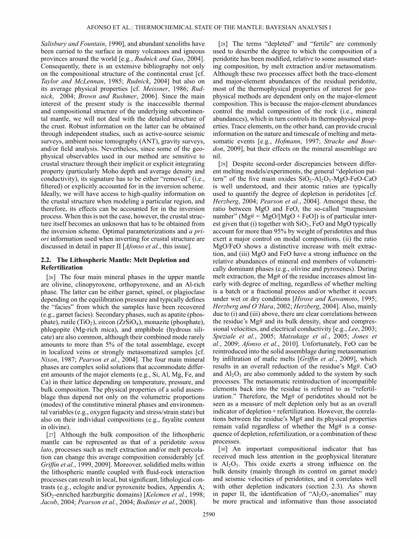
only one model parameter m0; if the observed data d(m0)are extremely sensitive to variations of this target parameter,and our physical theory describing the problem is exact, thenthe likelihood function L(m0) will have a very narrow peakabout the true value of m0, and so will � (m0) (Figures 1aand 1b). In this case, the true value of m0 is easily recov-ered (with high probability), regardless of the poor qualityof our prior knowledge �(m0). Conversely, if d(m0) is insen-sitive to m0 (Figures 1c and 1d), the posterior PDF, � (m0),will be entirely determined by our a priori information onm0. In reality, we typically deal with intermediate situa-tions in which our prior knowledge is somewhat vague, thephysical theory imperfect, and the sensitivity of geophysi-cal observables to some or all parameters of interest is oftennonlinear and relatively weak. Although L(m) usually canbe determined in a straightforward manner, the choice of�(m) is not trivial and often controversial [e.g., Scales andTenorio, 2001; Kitanidis, 2011a,2011b]. In essence, �(m)has to describe (i) everything we know about the problemthat is independent of the observed data and (ii) how cer-tain we are about this knowledge. This prejudice can affect(bias) our evaluation of � (m) to a large extent when theobservables at hand are not strongly sensitive to changes inmodel parameters.
[23] This paper focusses on the information that controlsthe estimations of L(m) and �(m) during the inversion ofgeophysical data for the thermochemical structure of thelithosphere and sublithospheric upper mantle. The likeli-hood function L(m) depends not only on the chosen data(i.e., geophysical observables), their associated uncertain-ties, and their intercorrelations but also on the physicaltheory relating these data to model parameters; the prior�(m) is controlled by our current understanding of mantlecomposition, thermal state, and thermophysical properties.An accompanying paper [Afonso et al., part II, this vol-ume] discusses in detail the general inversion methodologyin full 3-D geometry, its computational implementation(LitMod_4I), and synthetic examples. Readers interested in
the entire methodology will benefit from reading parts I andII together. The application of the method to a real-case sce-nario will be presented in a forthcoming publication [Afonsoet al., part III].
2. The A Priori Information: CompositionalParameters
[24] Any information about the model parameters anddata acquisition/processing that is independent of the actualresults of measurements (i.e., data values) can be treated asa priori information. It is customary in geophysical stud-ies to distinguish between a priori information on modelparameters m and on observable parameters d or data. Theformer often consists of an idea or prejudice about possi-ble distributions and associated uncertainties for the modelparameters, while the latter is related to the uncertaintiesaffecting the actual measurements. We refer the reader toDuijndam [1988] and Tarantola [2005] for more detaileddiscussions. We note here, however, that when a joint PDF�(d, m) = �M(m)�(d) can be defined, the prior PDF �(d)becomes part of the likelihood function L(m) (equation (7))[Mosegaard and Tarantola, 2002]. Therefore, we will dealwith this PDF when discussing L(m) in context of the actualdata and geophysical observables. In this section, we focuson the definition of the compositional parameters includedin our vector m, their associated �(m), and how to explorethem (by generating random and statistically independentsamples) in an efficient manner.
2.1. The Crust: Independent Information[25] Being the shallowest solid layer of the Earth, the con-
tinental crust has been extensively studied by geochemical,geophysical, petrological, and structural means. Entiresections down to lower crustal levels are accessible todirect observation/sampling in many orogenic belts [cf.
Likelihood L(m0)
a priori PDF ρ(m0)
parameter m0
parameter m0
parameter m0
parameter m0
true value of m0
posterior PDF σ(m0)
true value of m0
Likelihood L(m0)
a priori PDF ρ(m0)
true value of m0
posterior PDF σ(m0)
true value of m0
high
pro
babi
lity
high
pro
babi
lity
a b
c d
Figure 1. The posterior PDF is proportional to the product of L(m0) and �(m0). (a and b) Case wherethe observable is strongly sensitive to variations in the target parameter (m0) and our prior informationon model parameters is poor. The posterior PDF is controlled by L(m0) and it offers a good estimate ofthe true value. (c and d) Case where our prior knowledge of the parameter space is incorrectly biasedtowards wrong values and the observable is weakly sensitive to variations in the target parameter (m0).The posterior PDF is controlled by our faulted prior information and therefore the posterior PDF providesa high probability to wrong values.
2589
AFONSO ET AL.: THERMOCHEMICAL STATE OF THE MANTLE: BAYESIAN ANALYSIS I
Salisbury and Fountain, 1990], and abundant xenoliths havebeen carried to the surface in many volcanoes and igneousprovinces around the world [e.g., Rudnick and Gao, 2004].Consequently, there is an extensive bibliography not onlyon the compositional structure of the continental crust [cf.Taylor and McLennan, 1985; Rudnick, 2004] but also onits average physical properties [cf. Meissner, 1986; Rud-nick, 2004; Brown and Rushmer, 2006]. Since the maininterest of the present study is the inaccessible thermaland compositional structure of the underlying subcontinen-tal mantle, we will not deal with the detailed structure ofthe crust. Robust information on the latter can be obtainedthrough independent studies, such as active-source seismicsurveys, ambient noise tomography (ANT), gravity surveys,and/or field analysis. Nevertheless, since some of the geo-physical observables used in our method are sensitive tocrustal structure through their implicit or explicit integratingproperty (particularly Moho depth and average density andconductivity), its signature has to be either “removed” (i.e.,filtered) or explicitly accounted for in the inversion scheme.Ideally, we will have access to high-quality information onthe crustal structure when modeling a particular region, andtherefore, its effects can be accounted for in the inversionprocess. When this is not the case, however, the crustal struc-ture itself becomes an unknown that has to be obtained fromthe inversion scheme. Optimal parameterizations and a pri-ori information used when inverting for crustal structure arediscussed in detail in paper II [Afonso et al., this issue].
2.2. The Lithospheric Mantle: Melt Depletion andRefertilization
[26] The four main mineral phases in the upper mantleare olivine, clinopyroxene, orthopyroxene, and an Al-richphase. The latter can be either garnet, spinel, or plagioclasedepending on the equilibration pressure and typically definesthe “facies” from which the samples have been recovered(e.g., garnet facies). Secondary phases, such as apatite (phos-phate), rutile (TiO2), zircon (ZrSiO4), monazite (phosphate),phlogopite (Mg-rich mica), and amphibole (hydrous sili-cate) are also common, although their combined mode rarelyamounts to more than 5% of the total assemblage, exceptin localized veins or strongly metasomatized samples [cf.Nixon, 1987; Pearson et al., 2004]. The four main mineralphases are complex solid solutions that accommodate differ-ent amounts of the major elements (e.g., Si, Al, Mg, Fe, andCa) in their lattice depending on temperature, pressure, andbulk composition. The physical properties of a solid assem-blage thus depend not only on the volumetric proportions(modes) of the constitutive mineral phases and environmen-tal variables (e.g., oxygen fugacity and stress/strain state) butalso on their individual compositions (e.g., fayalite contentin olivine).
[27] Although the bulk composition of the lithosphericmantle can be represented as that of a peridotite sensulato, processes such as melt extraction and/or melt percola-tion can change this average composition considerably [cf.Griffin et al., 1999, 2009]. Moreover, solidified melts withinthe lithospheric mantle coupled with fluid-rock interactionprocesses can result in local, but significant, lithological con-trasts (e.g., eclogite and/or pyroxenite bodies, Appendix A;SiO2-enriched harzburgitic domains) [Kelemen et al., 1998;Jacob, 2004; Pearson et al., 2004; Bodinier et al., 2008].
[28] The terms “depleted” and “fertile” are commonlyused to describe the degree to which the composition of aperidotite has been modified, relative to some assumed start-ing composition, by melt extraction and/or metasomatism.Although these two processes affect both the trace-elementand major-element abundances of the residual peridotite,most of the thermophysical properties of interest for geo-physical methods are dependent only on the major-elementcomposition. This is because the major-element abundancescontrol the modal composition of the rock (i.e., mineralabundances), which in turn controls its thermophysical prop-erties. Trace elements, on the other hand, can provide crucialinformation on the nature and timescale of melting and meta-somatic events [e.g., Hofmann, 1997; Stracke and Bour-don, 2009], but their effects on the mineral assemblage arenil.
[29] Despite second-order discrepancies between differ-ent melting models/experiments, the general “depletion pat-tern” of the five main oxides SiO2-Al2O3-MgO-FeO-CaOis well understood, and their atomic ratios are typicallyused to quantify the degree of depletion in peridotites [cf.Herzberg, 2004; Pearson et al., 2004]. Amongst these, theratio between MgO and FeO, the so-called “magnesiumnumber” (Mg# = MgO/[MgO + FeO]) is of particular inter-est given that (i) together with SiO2, FeO and MgO typicallyaccount for more than 95% by weight of peridotites and thusexert a major control on modal compositions, (ii) the ratioMgO/FeO shows a distinctive increase with melt extrac-tion, and (iii) MgO and FeO have a strong influence on therelative abundances of mineral end members of volumetri-cally dominant phases (e.g., olivine and pyroxenes). Duringmelt extraction, the Mg# of the residue increases almost lin-early with degree of melting, regardless of whether meltingis a batch or a fractional process and/or whether it occursunder wet or dry conditions [Hirose and Kawamoto, 1995;Herzberg and O’Hara, 2002; Herzberg, 2004]. Also, mainlydue to (i) and (iii) above, there are clear correlations betweenthe residue’s Mg# and its bulk density, shear and compres-sional velocities, and electrical conductivity [e.g., Lee, 2003;Speziale et al., 2005; Matsukage et al., 2005; Jones etal., 2009; Afonso et al., 2010]. Unfortunately, FeO can bereintroduced into the solid assemblage during metasomatismby infiltration of mafic melts [Griffin et al., 2009], whichresults in an overall reduction of the residue’s Mg#. CaOand Al2O3 are also commonly added to the system by suchprocesses. The metasomatic reintroduction of incompatibleelements back into the residue is referred to as “refertil-ization.” Therefore, the Mg# of peridotites should not beseen as a measure of melt depletion only but as an overallindicator of depletion + refertilization. However, the correla-tions between the residue’s Mg# and its physical propertiesremain valid regardless of whether the Mg# is a conse-quence of depletion, refertilization, or a combination of theseprocesses.
[30] An important compositional indicator that hasreceived much less attention in the geophysical literatureis Al2O3. This oxide exerts a strong influence on thebulk density (mainly through its control on garnet mode)and seismic velocities of peridotites, and it correlates wellwith other depletion indicators (section 2.3). As shownin paper II, the identification of “Al2O3-anomalies” maybe more practical and informative than those associated
2590

AFONSO ET AL.: THERMOCHEMICAL STATE OF THE MANTLE: BAYESIAN ANALYSIS I
with FeO and/or MgO contents when inferring upper man-tle compositional domains through inversion of multiplegeophysical observables.
[31] Another incompatible “element” that affects thephysical properties of the mantle is water. Water is twoto three orders of magnitude more soluble in melts thanin mantle minerals [cf. Hirschmann, 2006]. Consequently,considering typical water contents in mantle rocks (<200–400 ppm), melt extractions of only <10% can effectively“dry out” the residue, significantly increasing its electricalresistivity and viscosity relative to its hydrated counterpart[e.g., Karato, 2008; Jones et al., 2012]. Note, however,that the expected average water contents of <400 ppm insubcontinental mantle rocks do not affect other relevantphysical parameters (Vs, Vp, density) to any significantextent (Appendix B).
[32] Another side effect of melt extraction is the removalof the highly incompatible radioactive elements K, Th, andU from the lithospheric mantle. The total contents of theseheat-producing elements determine the relative mantle con-tribution to the SHF and the temperature distribution withdepth in the lithosphere. Although it is usually expected thathighly depleted Archean xenoliths would have the lowestconcentrations of these elements, some compilations of cra-tonic, off-craton, and massif peridotite xenoliths [Rudnicket al., 1998] found an inverse correlation. These authorsinterpreted this “anomalous” behavior as being a conse-quence of several issues, such as postextrusion chemicalalteration, analytical detection limits, and sampling bias.However, Rudnick et al. [1998] concluded that the averagecontent of K, Th, and U from analyzed cratonic samplescannot be representative of the heat production of Archeanmantle roots. This indicates that melt extraction processes
are masked, in the case of these radioactive elements, byrefertilization processes, and therefore, the amount of meltextraction cannot be estimated or accounted for by meansof mass balance methods. Interestingly, anomalously highcontents of K, Th, and U in the lithospheric mantle, assuggested by some xenoliths, could locally increase thetemperature of the lithosphere above typical conductivegeotherms and produce detectable signatures in geophysicalobservables [Hieronymus and Goes, 2010].
2.3. Correlations Among Major Oxides[33] From the previous section, we can expect the major-
element contents of peridotites to be correlated to somedegree along melting or refertilization paths. In this section,we show that this holds true in real samples, which allows usto derive statistical correlations between the five main majoroxides in such a way that only two key element contents willbe needed as free compositional parameters in our inversionscheme in order to derive the entire set of thermophysicalproperties for a peridotitic rock.
[34] Figure 2 shows covariation plots of the main fiveoxides in peridotites from a large database (n > 2900)that includes xenoliths from both subcontinental lithosphericmantle (SCLM) and oceanic mantle as well as samplesfrom orogenic massifs and ophiolites (references in theSupporting Information). The Mg# of these samples rangesfrom � 84 to 96, thus covering most of the expectedvariability in mantle peridotites, from fertile (or refertil-ized) lithospheric mantle to highly depleted harzburgites anddunites from the Archean SCLM. Importantly, the negativecorrelation observed in the Al2O3-MgO and CaO-MgO plotsis one of the most robust features observed in peridotitesand is commonly interpreted as the result of either melt
30 35 40 45 50 5535
40
45
50
55
MgO
0
1
2
3
4
5
30 35 40 45 50 55
4
6
8
10
12
14
1
2
3
4
5
6
7
30 35 40 45 50 550
1
2
3
4
5
6
MgO
MgO
MgO
2
4
6
8
10
12
14
30 35 40 45 50 550
1
2
3
4
5
6
2
4
6
8
10
12
14
SiO
2
FeO
Al 2
O3
CaO
FeO
Al2O3 CaO
Figure 2. Covariation plots for our dataset (n > 2900). The color scales represent the content of a thirdoxide. Two polybaric perfect fractional melting paths [Herzberg, 2004] with different initial pressuresof melting are included for comparison; dashed line = 2 GPa, solid line = 7 GPa. The initial fertilecomposition for these melting paths is indicated by the white star.
2591

AFONSO ET AL.: THERMOCHEMICAL STATE OF THE MANTLE: BAYESIAN ANALYSIS I
depletion, late re-enrichment events, or a combination ofboth [cf. Griffin et al., 2009].
[35] Figure 3a shows a covariation plot of MgO andAl2O3 for our entire dataset. We have regressed the datawith both linear and polynomial models using a robustregression method based on an iterative weighted least-squares algorithm with a bisquare weight function[Rousseeuw and Leroy, 2003]. The final fitting modelobtained with this method is less sensitive to outliers in thedata as compared with ordinary least-squares methods. Thebest model was obtained with a second-order polynomialregression, which gives the lowest root mean square errorsand the highest R2 value (R2 = 0.772), respectively. A linearregression gives a R2 = 0.751, while higher-order poly-nomials overfit the data. Figure 3c also includes the 95%confidence interval of the predicted values. The meaning ofthis interval is straightforward. If one has a new sample forwhich the Al2O3 content is 3 wt%, then its MgO content hasa 95% probability of being between 37.5 and 42.5 wt% (i.e.,between the two confidence intervals). In addition, it is clear
from the data that the probability (or frequency) betweenthese two limits is not homogeneous, but it tends to follow aquasi-normal distribution. This is shown in Figures 3d and3e, which contain the frequency distribution for two Al2O3bins, each 1% wide. For comparison, Figures 3d and 3einclude two curves indicating the theoretical distributionsof two particular cases of the generalized Gaussian distri-bution: Laplacian (i.e., double exponential) and Gaussian(i.e., normal).
[36] A similar analysis can be applied to the covariation ofCaO and Al2O3 (Figure 4). In this case, there is no noticeableimprovement when fitting the data with higher-order modelsthan linear. The result of a robust linear regression is shownin Figure 4c, together with the two 95% confidence limits.As in the previous case, the distribution between these confi-dence limits is not homogeneous but follows a quasi-normaldistribution (Figures 4d and 4e).
[37] In contrast to CaO and MgO, SiO2 and FeO donot exhibit any significant correlation with either Al2O3 orCaO. Although the data show a tendency for SiO2 and FeO
0 1 2 3 4 5 630
35
40
45
50
55
α0 = 49.369 α1 = -4.106 α2 = 0.343
Al2O3
MgO = α0 + (α1 * Al2O3) + α2 * (Al2O3)2
0 1 2 3 4 5 630
35
40
45
50
55
Al2O3
Mg
O
CaO SiO2
0 1 2 3 4 5 630
35
40
45
50
55
Al2O3
1 2 3 4 5 6 7 38 40 42 44 46 48 50 52 54
R = 0.7722
a b c
34 36 38 40 42 44 46 48 50 520
20
40
60
80
100
120
140
160
34 36 38 40 42 44 46 480
10
20
30
40
50
60
70
80
MgO
Freq
uenc
y
Freq
uenc
y
MgO
1.0 < Al2O3 < 2.0 2.5 < Al2O3 < 3.5d e
Figure 3. Covariation plot of MgO with Al2O3 for all samples in our dataset. (a) Color scale indicates thecontent of CaO. (b) Color scale indicates the content of SiO2. (c) Results from a second-order polynomialrobust regression. Solid red line denotes the second-order polynomial fit; blue dashed lines denote the95% confidence limits from the regression. (d and e) Histograms of MgO content for two different Al2O3bins (from Figure 3a). The black solid lines are best-fitting Gauss (i.e., normal) distributions; the reddashed lines are best-fitting Laplace (i.e., double exponential) distributions. The 95% confidence limitsare shown as blue dashed lines.
2592

AFONSO ET AL.: THERMOCHEMICAL STATE OF THE MANTLE: BAYESIAN ANALYSIS I
0 1 2 3 4 5 60
1
2
3
4
5
6
Al2O3
CaO
MgO SiO2
0 1 2 3 4 5 60
1
2
3
4
5
6
Al2O3
34 36 38 40 42 44 46 48 50 38 40 42 44 46 48 50 52 54
0 1 2 3 4 5 60
1
2
3
4
5
6
CaO = α0 + α1 ∗ Al2O3 α0 = -0.164
α1 = 0.906
Al2O3
R = 0.6742
0 1 2 3 4 5 6 70
20
40
60
80
100
120
CaO
3.0 < Al2O3 < 4.0
Freq
uenc
y
0 1 2 3 4 5 6 70
10
20
30
40
50
60
70
80
CaO
2.0 < Al2O3 < 3.0
Freq
uenc
y
a b c
d e
Figure 4. Covariation plot of CaO with Al2O3 for all samples in our dataset. (a) Color scale indicatesthe content of MgO. (b) Color scale indicates the content of SiO2. (c) Results from a linear robust regres-sion. Solid red line denotes the linear fit; blue dashed lines denote the 95% confidence limits from theregression. (d and e) Histograms of CaO content for two different Al2O3 bins (from Figure 4a). Theblack solid lines are best-fitting Gauss (i.e., normal) distributions; the red dashed lines are best-fittingLaplace (i.e., double exponential) distributions. The 95% confidence limits are shown as blue dashedlines.
to increase with Al2O3 and decrease with MgO, in accor-dance with melting systematics, robust regression yields R2
values . 0.1 for both cases. This lack of correlation innatural samples reflects the interplay between mineral chem-istry, modes, and bulk composition. High-Mg olivine ororthopyroxene will have higher SiO2 contents (on a wt%basis) than the Fe-rich end member of each solid-solutionseries. On the other hand, in mantle peridotites, higher FeOcontents typically are found in more fertile rocks, whichwill have higher ratios of pyroxene (both opx and cpx) toolivine, raising SiO2 contents and countering the effect ofFe/Mg variations.
[38] Monte Carlo methods for sampling or exploring theparameter space of a model require the generation of manyrandom and statistically independent realizations (samples).For our purposes, such realizations will involve generatingrandom compositional samples (i.e., synthetic rock com-positions) within the system CaO-FeO-MgO-Al2O3-SiO2(CFMAS). In the most general case, we could define widelower and upper limits for the ranges of variation of each
oxide, assign a uniform probability density to all valueswithin this range, and then generate random samples for eachof them with the constraint that the sum of all five oxidesmust add to 100%. This approach would unavoidably samplethe entire parameter space, provided enough iterations areperformed, including those regions that are “empty” in thedata space (e.g., the region between 45 < MgO < 50 and 3 <Al2O3 < 4 in Figure 2). Conversely, when each oxide has adefinite and known probability distribution, we could samplethe compositional space much more efficiently by generatingsamples according to these distributions, thus avoiding over-sampling regions of low probability.
[39] In principle, the histograms in Figure 5 suggest pos-sible distributions. However, it is entirely possible, indeedlikely, that these distributions are the result of a samplingbias in existing databases, including ours. In particular,the double peaks in Al2O3 and CaO are controlled bythe Archean and Phanerozoic xenolith populations, whichtend to be numerically dominant in most global databases.This is simply because kimberlites, which preferentially
2593

AFONSO ET AL.: THERMOCHEMICAL STATE OF THE MANTLE: BAYESIAN ANALYSIS I
0 1 2 3 4 5 6 7 80
20
40
60
80
100
120
4 6 8 10 12 140
50
100
150
200
250
300
35 40 45 50 550
50
100
150
200
250
30 35 40 45 50 550
10
20
30
40
50
60
70
80
0 1 2 3 4 5 60
10
20
30
40
50
60
70
80
SiO2
MgO
FeO
Al2O3
CaO
Freq
uenc
yFr
eque
ncy
Freq
uenc
yFr
eque
ncy
Freq
uenc
y
0.3
0.2
0.1
PD
F
0.1
0.06
0.02
PD
F
0.1
0.3
0.5 PD
F
0.1
0.2
0.4
0.3 PD
F
0.1
0.2
0.4
0.3
PD
F
Figure 5. Histograms for the five major oxides in ourentire dataset (shown in Figure 2). Best-fitting densitydistributions are shown for each case. The latter havebeen calculated with a Gaussian kernel density estimator[Venables and Ripley, 1999]. If these probability densitieswere used to generate samples of the compositional space,samples with Al2O3 contents �1 would have much higherprobabilities than samples with Al2O3 contents >2. How-ever, this is a fictitious effect due to the dominance of“Archean” samples in the database (see text).
sample stable cratonic areas, and alkali basalts, which tendto sample young intraplate settings, are the most prolificsources of mantle xenoliths. By contrast, xenolith-rich vol-canic rocks are relatively rare in collisional settings (e.g.,island arcs), so these environments are under-represented inxenolith databases.
[40] There are other built-in biases in xenolith datasets.Alkali basalts typically sample shallow, less depletedmantle, with few samples from deeper than approximately60 km; garnet-bearing ultramafic xenoliths are rare or absentin most localities. Kimberlites typically sample down todepths of &180 km, but most studies of kimberlite-bornexenoliths have focussed on garnet-bearing samples, partlybecause they are amenable to P-T estimation; these xeno-liths are all from depths greater than approximately 80–100km. Shallower and/or more depleted (hence garnet-free) cra-tonic mantle is strongly under-represented in the publishedrecord. Published databases on kimberlite-borne ultramaficxenoliths also have been strongly dominated until recentyears by the abundant material from a small number ofkimberlites in the Western Terrane of the Kaapvaal Craton(Kimberley area), where mining has produced a veritablemountain of xenolith debris. Many of these samples arehighly enriched in orthopyroxene (high opx/oliv), and it hasbeen argued that the low FeO content of “average Archean”peridotites (Figure 2) simply reflects dilution by orthopy-roxene, rather than high-P melting [Simon et al., 2007;Pearson and Wittig, 2008]. However, the distinctive lowFeO contents of peridotite xenoliths from Archean cratonsare also observed in suites from North America, Siberia,and even other terranes of the Kaapvaal craton (e.g., N.Lesotho) where enrichment in orthopyroxene is not common[Griffin et al., 1999, 2009].
[41] Bearing in mind these considerations, any methodthat relies on a priori PDFs based on specific compilationsor on compositional/tectonic regionalizations (e.g., Archeandomains are assigned “Archean-like” compositions) can-not be considered entirely general. We therefore adopt asampling approach intermediate between the two extremesampling examples described above. Since statistically sig-nificant correlations between Al2O3 and CaO and Al2O3 andMgO are found in all published compilations of peridotiticsamples, regardless of their tectonic environment and/orfacies (see references in the Supporting Information), weassign more weight to these correlations (Figures 3 and 4)than to any specific univariate or multivariate probabilitydistribution (e.g., Figure 5). Therefore, in order to gen-erate random, statistically independent, and representativecompositional samples during our inversions, we proceedas follows:
[42] (i) Choose a wide initial variation range for Al2O3and FeO that covers >95% of the entire natural variability,and assign a uniform probability density within these ranges(i.e., equal probability to all values within the chosen range).Typically, we will use 0 < Al2O3 < 5.5 and 5 < FeO < 11(Figure 2), but these can be easily updated as more data isincluded in the database.
[43] (ii) Select a value for Al2O3 and FeO within theirrespective variation ranges using a random sampler.
[44] (iii) Use the selected Al2O3 value with the Al2O3-MgO and Al2O3-CaO regressions derived above (Figures 3
2594
AFONSO ET AL.: THERMOCHEMICAL STATE OF THE MANTLE: BAYESIAN ANALYSIS I
and 4) to obtain a preliminary (mean) value for MgO andCaO.
[45] (iv) Randomly select a new value for MgO andCaO from the known probability distributions associatedwith each Al2O3 value (Figures 3d and 3e and 4d and 4e).Typically, we will use a Gaussian distribution.
[46] (v) Calculate the SiO2 content of the present sampleas 100 – (FeO + CaO + MgO + Al2O3).
[47] This approach generates independent random sam-ples that cover the entire compositional spectrum observedin real mantle samples, without oversampling low-probability regions. Since it is based on well-establishedcorrelations between oxides (Figures 2–4) instead of whole-data PDFs (Figure 5), it is less sensitive to biases inthe dataset. Importantly, only two free parameters (Al2O3and FeO), instead of four, are needed in the random searchto obtain a complete representative compositional sample.As we show in paper II [Afonso et al., this volume], thisfeature is particularly useful when performing the full non-linear inversion in 3-D geometry, without compromising theresults to any extent in comparison to a full search withfour-free parameters.
3. Mineral Assemblages and InexactPhysical Theories
[48] As stated in section 1, the evaluation of the likelihoodfunction L(m) depends not only on the chosen observablesand their uncertainties but also on the physical theory usedto relate these observables to the model parameters. Theproblem of predicting the values of observable parame-ters d = (d1, d2, : : : dn) that would correspond to a certainmodel m = (m1, m2, : : :mn) is known as the forward prob-lem. In other words, the forward problem maps m into dthrough an operator g(�). This mapping, which can be non-linear, is usually written as d = g(m) [Tarantola, 2005].The operator g typically represents more than one physicaltheory (e.g., heat transfer and potential field), and the con-nection between them can be complex. In general, g willnot represent an exact (i.e., error-free) or perfect theory, andtherefore, it will be subject to modelization errors. However,the question of how to describe or quantify these errors is notstraightforward and depends on the actual theory and modeldiscretization (see below).
[49] In this work, the operator g is composed of suboper-ators associated with the solution of the following forwardproblems: Gibbs energy minimization gG, heat transfer gT,Maxwell’s equations gM, gravity potential gP, Love andRayleigh dispersion curves gD, and isostasy gI. An impor-tant part of the theoretical uncertainties associated with gG,gT, gI, and gM are intimately related to the actual physicaltheory (e.g., adopted solid-solution models, electrical con-ductivity as function of bulk composition, and local isostasyassumption) or assumed thermal parameters (e.g., radiogenicheat production and thermal conductivity), rather than to thediscretization of the model. Here, we discuss briefly the the-oretical uncertainties of gG, gM, gI, and gT that arise duringthe computation of the governing physical parameters (e.g.,electrical conductivity); those dominated by the discretiza-tion of the model and/or the numerical technique used tosolve the governing equations will be discussed in detail inpaper II.
3.1. Gibbs Energy Minimization (gG)[50] The thermodynamic (Gibbs energy minimization)
operator gG is used to obtain mineral assemblages frommajor-element compositions and given P-T conditions.The equilibrium mineral assemblages of all relevant ultra-mafic lithologies (i.e., eclogite, pyroxenites, and peridotites)and their relevant physical properties are computed withcomponents of the software Perple_X [Connolly, 2009]within the CFMAS system using the database and ther-modynamic formalism of Stixrude and Lithgow-Bertelloni[2011]. The CFMAS system accounts for &98 wt% ofthe Earth’s crust and mantle, and therefore, it is consid-ered to be an excellent starting basis for modeling phaseassemblages in the Earth. More complete systems, includ-ing, e.g., Na2O and H2O, can also be easily included inour method. However, as we show in Appendix B, theadded value of including additional elements in our compu-tations is insignificant when compared with the increase incomputational time.
[51] The estimation of the uncertainties associated withthe computation of the mineral assemblages (i.e., mineralmodes and their compositions) and their physical proper-ties can, in principle, be done by comparing laboratoryobservations with predictions. In practice, however, thisis problematic for two main reasons: (i) available labo-ratory “observations” on modal proportions of ultramaficrocks are subject to measurement uncertainties that are ofthe same order (sometimes significantly larger) as thoserelated to the modeling [cf. El-Hinnawi, 1966] and (ii)the lack of a large population of well-studied representa-tive mantle samples for which modal proportions, mineralchemistry, and physical properties have been measured withhigh precision at high P-T conditions. Typically, mineralmodes of real samples are estimated either by point-countingtechniques [cf. El-Hinnawi, 1966] or from bulk and min-eral chemical analyses by solving a least-square problemwith assumed density values for each phase. Although theuncertainties associated with these techniques depend onthe actual analyses and individual phase analyzed, val-ues between 1 and 3 wt% for two standard deviations arecommon. To illustrate the statement in point (i) above,we compare predicted and “observed” modal compositions(Table 1) for 10 representative xenoliths that span mostof the compositional range in our database (see also Afonsoand Schutt, 2012). In most cases, the difference betweenour predictions and the “observed” values is within theexperimental error, and when this is not the case, the dif-ference is negligible in terms of the associated changes inphysical properties.
[52] In this study, we use the standard Voigt-Reuss-Hillaverage for computing the elastic properties of the solidassemblage. A number of studies in which modes and elas-tic properties of polyphase materials have been measuredand compared with predictions from physical theories ofcomposites suggest that, as long as the modes are properlyaccounted for and the elastic parameters of the constituentphases are well known, predictions are typically within˙1.2% [e.g., Ji et al., 2003a; Ji, 2004; Afonso et al., 2005;Naus-Thijssen et al., 2011]. Interestingly, this value iscomparable to the differences between predictions fromstandard theories of composites and from different mineralphysics methods used to calculate the seismic properties of
2595

AFONSO ET AL.: THERMOCHEMICAL STATE OF THE MANTLE: BAYESIAN ANALYSIS I
Table 1. Comparison Between “Observed” and CalculatedModes for 10 Representative Samples From our Databasea
Sample phase obs. calc. �% 2STD
KGG13
Ol 68 68 0 2.48Opx 13 15 2 1.79Cpx 12 11 1 1.73Gt 7 6 1 1.36
KGG14
Ol 63 61 2 2.57Opx 11 14 3 1.66Cpx 10 9 1 1.60Gt 16 16 0 1.95
KGG06
Ol 72 71 1 2.39Opx 11 13 2 1.66Cpx 9 8 1 1.52Gt 8 8 0 1.44
KGG83
Ol 79 75 4 2.17Opx 9 14 5 1.52Cpx 5 5 0 1.16Gt 7 6 1 1.36
KGG88
Ol 72 68 4 2.39Opx 20 24 4 2.13Cpx 4 4 0 1.04Gt 4 4 0 1.04
FRB1684
Ol 69 72 3 2.46Opx 22 20 2 2.20Cpx 5 4 1 1.15Gt 4 4 0 1.04
FRB1685
Ol 63 65 2 2.57Opx 28 27 1 2.39Cpx 4 3 1 1.04Gt 5 5 0 1.16
PHN5304
Ol 73 76 3 2.36Opx 19 16 3 2.09Cpx 3 4 1 0.91Gt 5 4 1 1.16
PHN5316
Ol 60 60 0 2.61Opx 23 24 1 2.24Cpx 7 7 0 1.36Gt 10 9 1 1.60
U506
Ol 77 75 2 2.24Opx 16 18 2 2.01Cpx 3 3 0 0.91Gt 4 4 0 1.04
aThe thermodynamic database and formalism are that of Stixrude andLithgow-Bertelloni [2011]. All samples are garnet-bearing peridotites(KGG13, KGG14, KGG06, KGG83, and KGG88 from Franz et al.[1996]; FRB1684, FRB1685, PHN5304, and PHN5316 from Boydet al. [2004]; and U506 from Ionov et al. [2010], see references in theSupporting Information). �% is the absolute difference in modal per-cent between calculated and “observed” modes; 2STD is an estimationof the absolute error associated with the “observed” values (2 standarddeviations) computed as 1.85 � 0.6745
pk(100 – k)/n, where k is the
estimated mode of the phase in % and n the number of point counts,here assumed = 550 [El-Hinnawi, 1966].�% values larger than 2STDare shown in italics.
rocks [Ji, 2004; Schutt and Lesher, 2006; Afonso et al., 2008;Afonso and Schutt, 2012].
3.2. Electrical Conductivity of PolymineralicSamples (gM)
[53] Another important source of theoretical uncertaintyarises from the calculation of the electrical conductivity ofthe assemblage �. Several authors have recently reviewedthe connection between the composition and temperature of
peridotites, their water content, and their bulk electrical con-ductivity [e.g., Xu et al., 2000; Khan et al., 2006; Joneset al., 2009, 2012; Yoshino, 2010; Fullea et al., 2011, and ref-erences therein]. It is generally assumed that the dependenceof � on pressure, temperature, water content, and compo-sition for each phase can be adequately modeled by anequation of the form
� = �0 exp�
–�H(XFe, P)kBT
�+ �0i exp
�–�Hi
kBT
�
+ f (Cw) exp�
–�Hwet(Cw)kBT
�(8)
where kB is the Boltzmann constant and T the absolute tem-perature. The first to the third terms in the right-hand side ofequation (8) describe the contribution from small polarons(i.e., electron hopping and its associated lattice distortion),the contribution of Mg vacancies at high temperatures, andthe contribution by proton conduction (dependent on watercontent, Cw), respectively [cf. Jones et al., 2012 and ref-erences therein]. Pre-exponential parameters (�0, �0i, f (Cw))and activation enthalpies (�H(XFe, P), �Hi, �Hwet(Cw))are experimentally derived [cf. Jones et al., 2009; Fulleaet al., 2011].
[54] Fullea et al. [2011] have recently evaluated the cur-rent experimental discrepancies between different laborato-ries and their impact on the calculation of � for each phase.Using the maximum discrepancies between different exper-imental models of � as a proxy, we can assign the followingcompositional uncertainties to each phase: ��ol = 0.35for olivine; ��opx = ��cpx = 0.46 for clinopyroxene andorthopyroxene; and ��gt = 0.44 for garnet. Here, each ��represents a first-order estimate of the standard deviationassociated with log units (i.e., log(�)). The propagation ofthese phase uncertainties to the final estimation of the bulkrock electrical conductivity �T depends on the actual aver-aging method employed to calculate �T. Berryman [1995]and Jones et al. [2009] have discussed the available meth-ods for estimating the electrical conductivity of multiphasematerials and concluded that the Hashin-Shtrikman extremalbounds are the most reliable approach. In practice, the twoextreme bounds are rather similar and therefore their geo-metric mean can be taken as the best estimate of �T formost purposes. Using these equations and typical modalcompositions for peridotites, a standard error propagationanalysis results in a representative estimate of ��T � 0.4.Note that this value includes the uncertainty associated withtemperature (�0.3) [Xu et al., 1998].
[55] For the purposes of the present work, water contentCw will be considered known a priori and constant. Futurework will include Cw as an unknown to be retrieved from theinversion (Appendix B).
3.3. Isostasy and Elevation (gI)[56] The principle of isostasy is one of the oldest,
best-tested, and most powerful concepts in geophysics[cf. Turcotte and Schubert, 1982; Watts, 2001]. FollowingAfonso et al. [2008] and Fullea et al. [2009], we computeabsolute elevation under the assumption of local isostasy(see paper II for details). Except in regions of strong mantle
2596
AFONSO ET AL.: THERMOCHEMICAL STATE OF THE MANTLE: BAYESIAN ANALYSIS I
upwellings or subduction zones, local isostasy provides tightconstraints on the average (integrated) mass of lithosphericcolumns with areas & 1 � 104 km2 [Lachenbruch andMorgan, 1990; Turcotte and Schubert, 1982]. This holdstrue even when the wavelength of the density anomaly is lessthan 250–300 km, since corrections for flexural support canreadily be made when gravity anomalies are available [e.g.,Fullea et al., 2009].
[57] It is common in the literature to distinguishbetween crustal, thermal, and dynamic compensationmechanisms [cf. Phillips and Lambeck, 1980; Turcotteand Schubert, 1982; Nakiboglu and Lambeck, 1985;Lachenbruch and Morgan, 1990; Zhong, 1997; Hasterokand Chapman, 2007], depending on the nature of the densityanomaly compensating the associated topography. Of thesethree isostatic mechanisms, the first two typically accountfor more than 85% of the global surface elevation, regard-less of whether local or regional isostasy assumptions areused in the computations [Phillips and Lambeck, 1980;Mooney and Vidale, 2003; Kaban et al., 1999; Fullea et al.,2009]. In crustal isostasy, the density contrasts controllingelevation are those between mantle and crustal rocks atthe Moho and between air (or water) and surface topogra-phy. Thermal isostasy, on the other hand, refers to changesin topography due to temperature anomalies (strictly, tothe associated thermal expansion) in all or parts of thelithosphere (not only in oceans!). When the lithosphereis defined as a thermal boundary layer, the terms thermalisostasy and lithospheric isostasy can be used interchange-ably. Sublithospheric processes, such as plume impingementor forced convection, or intralithospheric processes, such asmantle delamination, can also modify surface topographythrough the generation and transfer of viscous stresses tothe surface (the so-called “dynamic effects”) [e.g., Marquartand Schmeling, 1989; Lithgow-Bertelloni and Silver, 1998;Petersen et al., 2010]. Results from convection simulationsindicate peak dynamic contributions to the total topogra-phy of the order of �400–800 m [Marquart and Schmeling,1989; Crameri et al., 2012] for relatively large plumes.However, these estimates need to be taken with caution,since convection computations rely on relatively uncertainparameters (e.g., asthenosphere viscosity and lithosphericstrength) and in some cases, inaccurate numerical schemes[cf. Crameri et al., 2012].
[58] Considering all of the above, we assign an averagetheoretical uncertainty of 15% to our computed elevation(with a minimum uncertainty of˙200 m), except in regionswhere evidence for large dynamic loads exists. In this case,higher local uncertainties or appropriate topographic correc-tions should be used.
3.4. Thermal Conductivity and RadiogenicHeat Production (gT)
[59] The main physical parameters controlling resultsfrom forward thermal modeling of the lithosphere are theradiogenic heat production RHP and thermal conductivitykt of the rocks. Both these parameters are known to varywithin relatively large ranges when different lithologies areconsidered. In particular, kt of the main silicate mineralscan vary from �1.6 to >7 W m–1 K–1 at room P-T con-ditions, although �90% of typical rocks exhibit kt valuesof 2–4 W m–1 K–1 [cf. Diment and Pratt, 1988; Clauser
and Huenges, 1995; Jokinen and Kukkonen, 1999; Jaupartand Mareschal, 2011]. Likewise, although RHP of typicallithospheric rocks can vary by as much as �0 to >10 �Wm–3 between individual samples, regional averages (moresuitable for lithospheric studies) are typically limited toRHP values <3.6 �W m–3 [Vilá et al., 2010; Jaupart andMareschal, 2011]. Using Monte Carlo simulations, Jokinenand Kukkonen [1999] showed that if the thermal conductiv-ity and RHP of crustal layers can be estimated with standarddeviations of 0.5–1.0 W m–1 K–1 and �2 �W m–3, respec-tively, then the uncertainty in calculated temperatures withinthe lithosphere would amount to˙45–80ıC. The uncertain-ties associated with calculated values of SHF, as estimatedby these authors, are of the order of ˙6–15 mW m–2. Com-parable, although somewhat larger, values were recentlyestimated by Vilá et al. [2010]. It therefore seems reasonableto assign minimum uncertainties of ˙80ıC and ˙10 mWm–2 to temperature and SHF predictions from gT, respec-tively. We will typically use the same uncertainty values fortemperatures at sublithospheric depths.
3.5. Putting Everything Into � (d | m)[60] With the above considerations, and in lieu of more
detailed information, we ignore the uncertainty in the com-putation of mineral modes and phase composition associatedwith gG, since it is the smallest estimated uncertainty. Forpredictions of the aggregate’s seismic properties, �, temper-ature, elevation, and SHF, we will assume Gaussian PDFs ofthe form (refer to equation (7))
� (d | m) =/ exp�
–12
(d – g(m))TC–1t (d – g(m))
�(9)
where Ct is the covariance matrix describing the theoreti-cal uncertainties. It is also expected that a certain amountof correlation exists between these theoretical uncertainties.We address these correlations and the computation of thefull-rank Ct in paper II.
[61] An important problem that arises when calculatingseismic velocities is the estimation of anelastic effects athigh temperatures. Anelasticity in mantle rocks, and theassociated attenuation of seismic waves, become impor-tant at temperatures >900ıC [e.g., Jackson et al., 2002;Jackson and Faul, 2010] . Since all of the sublithosphericupper mantle and up to �40% of the SCLM have tempera-tures higher than this limit, a correction to the anharmonicvelocities obtained from the minimization problem is neces-sary. Unfortunately, experimental studies at relevant seismicfrequencies and P-T conditions addressing the effects ofgrain sizes, volatile content, and bulk composition are eitherscarce or nonexistent. Moreover, meaningful comparisonsbetween mineral physics models and observations are prob-lematic due to the uncertainties affecting observations ofseismic attenuation [e.g., Dalton and Faul, 2010] and, moreimportantly, the uncertainties in the average grain size andtemperature structure of mantle sections. All these makeit difficult, if not impossible, to objectively quantify thetheoretical error associated with anelastic corrections. Afirst-order estimation of this error and its implementation inCt are discussed in paper II.
2597

AFONSO ET AL.: THERMOCHEMICAL STATE OF THE MANTLE: BAYESIAN ANALYSIS I
4. Geophysical Observables: Sensitivity andObservational Uncertainties4.1. Two Levels of Functional Relationships
[62] The fundamental goal of this study is the conver-sion of observations into robust estimates of temperatureand composition in the lithosphere and sublithospheric uppermantle. This requires the assessment of two different butrelated levels of functional relationships (or parameteriza-tions). The first is between the raw observations and theset of governing physical parameters, e.g., the physicalrelationship between travel times and the subsurface seis-mic velocity structure or between variations in the surfaceelectromagnetic field and the subsurface electrical conduc-tivity structure. The second level of functional relationshipis between the set of governing physical parameters (e.g.,seismic velocity) and a more fundamental set of modelparameters represented by the major-element composition,pressure, water content, and temperature of the aggregate.Since this set of fundamental parameters (e.g., composition)controls the second set of governing physical parameters(e.g., shear velocity), they are commonly referred to asthe primary and secondary parameters, respectively [Bosch,1999; Khan et al., 2007].
[63] The first level is the simplest and most widely usedin conventional inversion methods. Typically, an appropriatephysical theory (e.g., seismic wave propagation) is assumedand used to relate the secondary model parameters to theobservations during the inversion. The final result is one ormore sets of secondary physical parameters (i.e., Earth mod-els), such as shear velocity or electrical conductivity, whichexhibit an acceptable data fit. The second level of func-tional relationships is commonly ignored in inversion studiesor treated as a posteriori independent (not self-consistent)corrections. Partly because of this, but also due to its intrin-sic complexities (e.g., different compositions give the sameseismic velocity), this functional level and its relationshipwith different geophysical observables in joint inversions area less well-understood subject.
[64] In the following, we address both levels by dis-cussing (i) the strengths and weaknesses of our choice ofgeophysical observables as well as their experimental uncer-tainties (section 4.2) and (ii) the intrinsic sensitivities ofthe secondary parameters Vs, Vp, bulk density, and � tochanges in the primary parameters in peridotitc assemblages(sections 4.3 and 4.4).
4.2. The Need for Multiple Observables[65] The main purpose of inverting multiple geophysical
observables is to minimize the range of acceptable mod-els consistent with data. In other words, we aim to reducethe number of acceptable solutions to the inverse problemby taking into account more constraining data. It is there-fore not only desirable but necessary that each piece ofinformation (e.g., a new observable) newly added to the sys-tem has a different sensitivity to the model parameters ofinterest. If a new constraining dataset is added to the inver-sion, but its sensitivity to model parameters is similar to,or less than, that of the existent data, the inversion willnot provide new information about the state of the system.In this work, we will combine information from grav-ity and geoid anomalies, seismic velocities, SHF, absolute
elevation, and magnetotelluric data. We have purposelychosen these geophysical observables because they are dif-ferently sensitive to shallow/deep, thermal/compositionalanomalies, which allows superior control over the lateral andvertical variations in the mantle’s bulk properties. From aBayesian point of view, what we want to achieve by includ-ing different datasets in a probabilistic inversion is to narrowthe likelihood function L(m) towards “good” values. How-ever, the form of L(m) is largely controlled by the form of�(d), which in turn is controlled by the nature of the chosengeophysical observables, their associated uncertainties, andtheir intercorrelations (equations (7) and (9)). In this section,we discuss in detail the first two. The intercorrelationsbetween uncertainties (both theoretical and observational)are addressed in paper II.4.2.1. Gravity and Geoid Data
[66] Gravity and geoid anomalies are arguably thesimplest and most commonly used geophysical observ-ables for investigating lithospheric features [Zeyen andFernàndez, 1994; Zeyen et al., 2005; Ebbing et al., 2006;Jiménez-Munt et al., 2008; Chappell and Kusznir, 2008;Kaban et al., 2010; Watts, 2001; Jacoby and Smilde, 2009,amongst others]. Unfortunately, given the 1/r2 dependenceto the depth of the density anomaly, their sensitivity totypical lithospheric density anomalies decays to almostnil at depths &50 km, except for large-scale anomalieswith unusual density contrasts (e.g., continent-ocean bound-ary, Trans-European Suture Zone). Nevertheless, satellite-derived gravity anomalies offer one of the best spatialcoverages of all available observables and can be used toput strong constraints on possible short-wavelength densitydistributions for the shallow lithosphere, especially whenthey are combined with seismic information [e.g., Korenagaet al., 2001; Roy et al., 2005]. For example, gravity anoma-lies are particularly suited to estimating the structure ofthe Moho and the elastic thickness of the lithosphere [cf.Watts, 2001; Jacoby and Smilde, 2009]. Their measurementuncertainties are typically low, varying between 2 and 10mGal in global databases [Sandwell and Smith, 2009] tobetween 0.1 and 0.01 mGal in regional surveys.
[67] When the density anomaly is broad and deeper thanaround 50 km (e.g., within the SCLM), its signature in grav-ity anomalies becomes small and therefore, it is difficult toisolate the effects of the deep anomaly from those of othershallower anomalies, which dominate the signal. In this case,geoid anomalies (perturbations of the gravity potential) canprove a better constraint on the depth distribution of den-sity due to their sensitivity to nonzero density moments[Turcotte and Schubert, 1982]. These characteristics makegeoid anomalies better suited than gravity anomalies for con-straining deep density anomalies, e.g., those arising fromvariations in the LAB (Appendix C). Uncertainties associ-ated with recent geoid height models are extremely low,usually <5 cm accuracy down to 275 km half-wavelength[e.g., Reigber et al., 2005]. Modelization errors (e.g., fil-tering and discretization) are therefore the largest source ofuncertainty when fitting geoid heights (see paper II).4.2.2. Surface Wave Data
[68] Phase velocity dispersion maps obtained from thecombination of ANT with teleseismic surface wave tomog-raphy constitute one of the best sources of informationfor retrieving absolute Vs values in the lithosphere and
2598

AFONSO ET AL.: THERMOCHEMICAL STATE OF THE MANTLE: BAYESIAN ANALYSIS I
sublithospheric upper mantle [Yang et al., 2008]. The mainadvantage of this method is that while ANT providesdetailed information at short periods (shallow levels), tele-seismic earthquake methods such as multiple-plane-wavetomography (MPWT) [Yang et al., 2008] provide the com-plementary information at longer periods (deep levels). Theability to recover “good” values of Vs, however, dependson the uncertainties associated with the phase velocity dis-persion maps generated by each method. In the case ofANT, robust estimations of the uncertainties in phase veloc-ity maps can be obtained by the method of local Eikonaltomography [e.g., Lin et al., 2009]. This method constructsa phase travel time map centered on each station of a seis-mic array by tracking phase travel times measured fromcross-correlations of ambient noise between each stationand all other stations within the seismic array. Each station-centered phase time map is then converted (separately) toa phase velocity map based on the Eikonal equation [e.g.,Shearer, 1999]. The final phase velocity map is obtained byaveraging all the individual phase velocity maps centered atdifferent stations, and associated phase velocity uncertain-ties are estimated from the variations of multiple station-centered phase velocity maps. Lin et al. [2009] applied thisapproach to the EarthScope/US Array and showed that theperiod-averaged uncertainties associated with their disper-sion maps typically average to <10 m/s for stations locatedin the middle of the array and �20 m/s for stations nearthe edges. Phase velocity uncertainties estimated in this waydepend mainly on the quality of the travel time data and onthe total number of stations in the seismic array.
[69] In the case of MPWT, uncertainties are estimatedfrom the a posteriori model covariance matrix after solv-ing the nonlinear least-squares problem [Yang and Forsyth,2006].
�m =�GTC–1
nnG + C–1mm�–1 �GTC–1
nn�d – C–1mm[m – m0]
�(10)
where m0 is the original staring model, m is the currentmodel, �m is the change relative to the current model, �dis the difference between the observed and predicted datafor the current model, G is the partial derivative of d withrespect to perturbations of m, Cnn is data covariance matrixdescribing the data uncertainties, and Cmm is the prior modelcovariance matrix, which acts to damp or regularize the solu-tion. A minimum length criterion is employed for dampingby assigning a typical prior model variance of �0.2 kms–1 for phase velocity parameters to the diagonal term ofCmm and leaving all the off-diagonal terms to zero. For astudy region with dense station coverage and sufficientlylong duration of deployment, such as the US continent cov-ered by the USArray, the choice of different damping valueshas only marginal effects on both phase velocity maps anduncertainties. In such cases, the uncertainties of data (i.e.,surface wave phase and amplitude) are evaluated using anaverage data misfit for each event. Applying this method tothe USArray data in Western USA, Yang et al. [2008] esti-mated period-averaged uncertainties of 10–15 m/s at stationsnear the center of the array. For other arrays/study regions,however, the effects of different damping parameters maynot be marginal and thus, they need to be evaluated for thatparticular method and array (e.g., the choice of dampingin MPWT could be gauged by comparing resulting phase
velocity maps from MPWT at overlapped periods with thosefrom Eikonal tomography, which does not require dampingin obtaining phase velocity dispersion curves).
[70] With uncertainties of phase velocity maps both beingable to be estimated for ANT and MPWT, one can thenestimate uncertainties in Vs via Monte Carlo methods [e.g.,Yang et al., 2008]. In the case of the USArray data, thepropagation of the uncertainties in the dispersion maps men-tioned above results in uncertainties of 0.05–0.07 km/sin the absolute Vs structure of the mantle [Yang et al.,2008]. It is worth noting that the above uncertainty esti-mates are valid only for the particular method discussedhere, when using the dense USArray dataset. This exem-plifies the ideal case for the sort of inversions described inthis work. These uncertainties are not intended to be repre-sentative of the whole range of velocity models that wouldarise from the application of different methods. Specificuncertainties should be estimated from the particular methodused to obtain the dispersion data rather than by comparingresults from different methods (we do not use a mixture ofresults/data/methods).4.2.3. Body Wave Data
[71] Body wave data have been used extensively to mapthe lithosphere and upper mantle structures for over threedecades. Most regional body wave tomography use P-waveand/or S-wave travel time residuals that are calculated rela-tive to a 1-D reference model to constrain Vp and/or Vs val-ues of the lithosphere and sublithospheric upper mantle [e.g.,Rawlinson et al., 2006; Shomali et al., 2006]. In a regionaltomography, earthquakes are typically located outside thestudy region and therefore, in order to remove source patheffects, the resulting Vp model is usually a model of velocityperturbation rather than an absolute velocities. This meansthat in order to obtain estimates of temperature and com-position, one needs to first convert velocity anomalies intoabsolute velocities by superimposing the anomalies on thebackground reference model. However, using different ref-erence models in body wave tomography commonly resultsin similar perturbation models; in other words, different ref-erence models do not significantly affect the anomaly model.Thus, absolute velocity models based on regional body wavetomography only are not robust.
[72] In addition, due to differences in the methodologiesand parameterizations/regulations used by different researchgroups, body wave anomaly models tend to be considerablydifferent, even when using similar input data. For instance,Becker [2012] has recently compared several Vp models ofwestern USA constructed from P-wave travel times recordedat the dense and broad USArray. This author found that,although the pattern of anomalies at scales �200 km isremarkably consistent between different models, significantdifferences in both amplitudes and small-scale patterns arethe rule rather than the exception. Differences of several per-cent in the amplitudes of the anomalies are common betweendifferent models [Becker, 2012]. Such discrepancies are ofthe same order, if not larger, than those expected from largeand moderate compositional and thermal anomalies, respec-tively. This illustrates an important limitation of body wavetomography as a direct proxy for compositional and thermalanomalies in the lithosphere.
[73] Within the present Bayesian framework, an attrac-tive alternative that we discuss in paper II is to include
2599

AFONSO ET AL.: THERMOCHEMICAL STATE OF THE MANTLE: BAYESIAN ANALYSIS I
teleseismic arrival time residuals into the data vector dtogether with an additional operator gtt used to computesynthetic travel time residuals [Rawlinson and Sambridge,2004; Rawlinson et al., 2006]. Although this adds a newset of uncertainties to the problem (those associated withobserved and computed arrival times), it does guaranteethat the absolute velocity model used to compute traveltime residuals is simultaneously (and thermodynamically)consistent with dispersion data as well as with all otherobservables. This is, in itself, an important step forward forjoint inversions. In this context, the uncertainties associatedwith arrival times are important to judge whether a model isacceptable or not under the framework of a Bayesian inver-sion. However, travel time uncertainties are notoriously hardto estimate, and thus most body wave tomography studiesdo not address the problem. Based on the few studies thatattempted to estimate realistic uncertainties [e.g., de Wit etal., 2012; Gudmundsson et al., 1990; Amaru et al., 2008],values of 0.5–1 s seem reasonable for large-scale studies.When dense local seismic networks are used instead, uncer-tainties associated with relative arrival time residuals can be,in average, less than 0.1 s [e.g., Rawlinson et al., 2006].4.2.4. Magnetotelluric Data
[74] Experimental uncertainty in magnetotelluric datacomprises two types, random error and bias error. Randomerrors are well known and well understood, and modernjackknife-based methods give appropriate error estimateson the MT impedance tensor elements without assumptionsabout the distributions of the estimates [e.g., Chave andJones, 1997; Eisel and Egbert, 2001; Chave, 2012]. High-quality data can usually be acquired with random errors oforder 1% of the impedance values. In many places, however,the data errors are larger, mostly as a consequence of highnoise disturbances (DC trains etc.). Also, long period sig-nals can be lower, as signal strength is directly related to the11-year sunspot cycle.
[75] Far more difficult to quantify are bias errors thatare caused by distortion effects [e.g., Jones, 2012]. Thesetake two forms, either galvanic distortion that can lead par-ticularly to errors in primarily the magnitudes of the MTimpedances or inadequate dimensionality assumption, i.e.,interpreting 2-D data using 1-D methods or 3-D data using 2-D (or 1-D) methods. For the latter, there are dimensionalitytests that can be performed, and the one in most current use isthe Groom-Bailey approach [Groom and Bailey, 1989], par-ticularly the multisite, multifrequency code of McNeice andJones [2001]. For the former, there are approaches in use tocontrol the indeterminable part of distortion, the so-called“static shifts” [Jones, 1988]. Generally, for high-quality MTdata that are appropriately treated, experimental uncertaintyis of order some 1–2% of the impedance values.
[76] The mapping from experimental errors into modelerrors is difficult and fraught with high potential for misun-derstanding. Although there exists a uniqueness theorem in1-D and one of the 2-D modes for perfect MT data at all fre-quencies [Bailey, 1970], for real data with error, one must becognizant of the issues. The functional relationship betweenconductivity and observed response is highly nonlinear, andagain, there are random errors and bias errors. Randomerrors can be quantified through linearized approaches, suchas that of Schwalenberg et al. [2002] in two dimensions(2-D). Bias errors are far more difficult to quantify and
relate mainly to the insensitivity of inductive methods tothe resistivity of a resistive region, where “resistive” and“conductive” are relative terms. For example, the resistivityof the uppermost mantle directly below the crust is typi-cally impossible to determine accurately due to the presenceof conducting material in the lower crust [see, e.g., Jones1999, figure 3]. Only in cases where the crust is resistivefor its entire depth extent is it possible to determine theabsolute resistivity of the uppermost mantle [e.g., Jones andFerguson, 2001; Ledo et al., 2004]; otherwise, a minimumbound can be set for the resistivity, but not a maximumbound. Regularization errors will be discussed in paper II.4.2.5. Absolute Elevation
[77] Observational uncertainties associated with elevationare low, amounting to .15 m in high-resolution (30 arc sresolution) global databases [Becker et al., 2009]. In ourinversions, however, the area of the individual columns issufficiently large (�2500–10,000 km2) to include significantlocal variations in elevation that need to be averaged to asingle value with a representative uncertainty. We do this bycalculating the mean and standard deviation of the individualdata points within each column. In most cases, the standarddeviations so obtained are .150 m.4.2.6. Surface Heat Flow
[78] Surface heat flow measurements are expensive, par-ticularly in continents, and therefore they are scarce andheterogeneously distributed [e.g., Davies and Davies, 2010].In addition, SHF values are typically dominated bythe heat production of the crust and are significantlyaffected by shallow advection processes; their sensitiv-ity to deep mantle thermal anomalies is strongly dimin-ished when these are located at depths >180 km [cf.Jaupart and Mareschal, 2011]. For these reasons, litho-spheric/sublithospheric models based purely on SHF dataare not considered to be reliable. Despite these limitations,SHF nevertheless provides some constraints, albeit weak,and can be a useful “secondary” observable when dealingwith the mantle thermal structure. By secondary we meanthat, although the relative weight assigned to SHF duringthe inversion is low in comparison with other observables(e.g., seismic waves), any acceptable model of the litho-sphere/sublithosphric upper mantle must be consistent withSHF data as well.
[79] Typical uncertainties associated with SHF measure-ments in continents amount to˙5–10 mW m–2 [e.g., Powellet al., 1988], which is equivalent to a depth change in theLAB of �50 km (if the LAB is defined as an isotherm, e.g.,1300ıC). However, this equivalency is strictly valid only ifthe LAB change is confined to a depth range between �60and 180 km. At 250 km depth, an identical change in depthtranslates into a SHF change of only 5–8 mW m–2.4.3. Dependence of Physical Parameters onMajor-Element Composition4.3.1. An Illustrative Example
[80] Let us assume that we have laboratory measurementsof the (secondary) parameters Vs, Vp, electrical conductiv-ity �, and bulk density for a peridotite sample at P = 3 GPaand T = 900 ıC (assume that Vs and Vp are high-frequency,unrelaxed, velocities). Our task is to retrieve the truemajor-element composition of the sample by exploring theentire compositional space with a Monte Carlo method and
2600

AFONSO ET AL.: THERMOCHEMICAL STATE OF THE MANTLE: BAYESIAN ANALYSIS I
32 34 36 38 40 42 44 46 48 50 5235
40
45
50
55
32 34 36 38 40 42 44 46 48 50 525
6
7
8
9
10
11
32 34 36 38 40 42 44 46 48 50 520
1
2
3
4
5
6
32 34 36 38 40 42 44 46 48 50 520
1
2
3
4
5
6
5 15 25 35 45
MgO
MgO
MgO
MgO
CaO
Al2
O3
SiO
2
FeO
|predicted Vs - observed Vs| [m/s]
n = 2382
Mg# = 88
Mg# = 90
Mg# = 92
Figure 6. Ensemble of 2382 acceptable compositions from a total random population of 2500 samples.The only constraining parameter is the Vs velocity. The true (target) composition is indicated by the whitestar (SiO2 = 44.03, Al2O3 = 3.81, FeO = 8.08, and MgO = 40.82, CaO = 3.25) and the correspondingtarget Vs velocity is 4.634 km s–1 (calculated at T = 900 ıC, P = 3 GPa). The color scale representsthe misfit in absolute values. The sampling is performed following the steps explained in the text andtruncating the samples at the 95% confidence limits.
comparing our predictions to the observed parameters. Pre-dicted values of Vp, Vs, �, and bulk density for all testedcompositions are obtained by solving the Gibbs energy mini-mization problem (section 3.1). To make a (much simplified)comparison with real-case scenarios easier, further assumethat the measurements have associated uncertainties in Vsand Vp comparable to those from dense surface wave andrefraction studies (˙52 and ˙82 m s–1 for Vs and Vp,respectively). We warn the reader that these uncertainties,although realistic, are strictly valid for the present illustrativeexample only. More appropriate values (particularly for Vpand dispersion curves) will be used in a real 3-D inversion(paper II).
[81] We generate sets of 2500 random compositional sam-ples each, using the method described in section 2.3 (thisnumber is sufficient to sample well the entire compositionalfield indicated by real samples; Figure 2). During each sim-ulation, we save a subset containing the samples that fit thedata within their defined uncertainties. This subset then con-stitutes an ensemble of acceptable samples. Figure 6 showsthe result of one such simulations in which Vs is the onlyconstraining parameter. All samples in this subset fit the trueVs value within ˙52 m s–1 (the assumed uncertainty). Notethat the assumed uncertainty is close to the low end of repre-sentative uncertainty values in high-resolution surface wavestudies (section 4.2.2), and thus, this example represents thebest possible scenario. Even when the uncertainty is reduced
by a factor of two (unrealistically good), the resulting subsetof samples consistent with the data still spreads over a largecompositional range. This simple exercise demonstrates thatVs alone defines neither the composition of our syntheticsample nor the fine compositional structure of the Earth’supper mantle; it only suggests that a peridotitic compositionsensu lato is compatible with the observed Vs value.
[82] When Vp is used as the only constraint, the subset ofacceptable samples is smaller than when using Vs, but theacceptable compositional range remains large (Figure 7). Inthis case, the samples of this subset fit the true Vp valuewithin ˙82 m s–1, which is again close to the low end oftypical uncertainties in refraction studies. The reason forthe reduction on the number of acceptable samples whenusing Vp instead of Vs is mainly due to the disappearanceof the “low-Al2O3” samples (yellow-red dots in Figure 6).This is because, at equal MgO contents, the bulk modulus ofthe assemblage is more sensitive to changes in bulk Al2O3(i.e., garnet mode) than the shear modulus. Therefore, theacceptable Al2O3 range for samples with an identical MgOcontent is narrower in Figure 7. However, as in the Vs case,the compositional range allowed by Vp is large enough toinclude most of the natural variability (Figure 2). Note thetwo regions of low misfit (blue dots) at high and low MgOcontents. The low-residual samples at the high-Mg end areharzburgites (opx + ol) and dunites (mostly ol) while thoseat low-Mg end are lherzolites (cpx + opx + ol + gte). When
2601

AFONSO ET AL.: THERMOCHEMICAL STATE OF THE MANTLE: BAYESIAN ANALYSIS I
32 34 36 38 40 42 44 46 48 50 5235
40
45
50
55
10 20 30 40 50 60 70 80
32 34 36 38 40 42 44 46 48 50 525
6
7
8
9
10
11
32 34 36 38 40 42 44 46 48 50 520
1
2
3
4
5
6
32 34 36 38 40 42 44 46 48 50 520
1
2
3
4
5
6MgOMgO
MgO MgO
CaO
Al2
O3
SiO
2
FeO
|predicted Vp - observed Vp| [m/s]
n = 1363
Mg# = 88
Mg# = 90
Mg# = 92
Figure 7. Ensemble of 1363 acceptable compositions from a total random population of 2500 sam-ples. The only constraining parameter is the Vp velocity. The true (target) composition is the same as inFigure 6 (white star) and the corresponding target Vp velocity is 8.185 km s–1 (calculated at T = 900 ıC,P = 3 GPa). The color scale represents the misfit in absolute values. Sampling method as in Figure 6.
larger uncertainties are considered (˙120 m s–1), the sub-set of acceptable samples is larger, but the two regions oflow misfit at high and low MgO contents remain. In theideal case of small uncertainty in the observed Vp value(˙10 m s–1), the diagram would show two separate clustersof acceptable samples, and independent information wouldstill be needed to decide on the composition of the sample. This two-branched pattern in Vp has been recognizedbefore [Afonso and Schutt, 2012] and reflects the competi-tion between modal (phase abundances) and chemical (com-position of the phases) effects in peridotites as their Al2O3and CaO contents decrease. As expected, fitting Vp andVs simultaneously (or their ratio) produces similar resultsas those in Figure 7, and therefore, we do not include anadditional figure.
[83] At first glance, these results seem to be at oddswith the strong correlations between Vp/Vs and Mg%found in several previous studies [e.g., Lee, 2003; Spezialeet al., 2005; Afonso et al., 2010]. However, although the cor-relations are a robust result, the actual application of them toinfer the Mg% of mantle domains is hampered by the unre-alistically low uncertainties required for Vp, Vs, and/or �.When realistic uncertainties associated with these propertiesare considered (e.g., ˙0.02 for Vp/Vs ratio), the range ofpossible Mg% as given by the above correlations becomeslarge enough to cover most of the natural range in peridotites[compare with Figure 2 in Afonso et al., 2010]. This is pre-cisely what Figures 6 and 7 highlight; the contradictions aretherefore only apparent.
[84] Assigning uncertainties to density data in the uppermantle is more problematic, since traditional geophysicalmethods are weakly sensitive to absolute density valuesat small scales (<250 km). For our present (illustrative)purposes, an objective uncertainty can be estimated basedon the discrepancies between predictions from differ-ent thermodynamic [Holland and Powell, 1998 (revised2002); Stixrude and Lithgow-Bertelloni, 2011], hybrid[Afonso et al., 2008], and mineral physics methods [Schuttand Lesher, 2006] for identical compositions. We have com-pared predictions from the methods of Schutt and Lesher[2006], Afonso et al. [2008], and Stixrude and Lithgow-Bertelloni, [2011] for identical samples and found that theirdiscrepancies amount to <1% for conditions pertaining tothe upper mantle [see also Afonso and Schutt, 2012]. Withthese estimates, a simulation using density as the only con-straint generates the subset of acceptable samples shownin Figure 8. Since bulk density is the bulk property thatcorrelates best with Mg#, the compositional range alongthe MgO and FeO axes has been reduced compared withthose from Vs or Vp. Also, at identical MgO contents, therange in SiO2 content has been reduced. This is due to thesignificant effect of the low-density phase Opx (which iscontrolled by the SiO2 content of the sample) on bulk den-sity. Despite these improvements, the compositional rangestill is too large to provide a definite composition forour sample.
[85] Electrical conductivity alone does not represent anyimprovement with respect to the other parameters (Figure 9),
2602
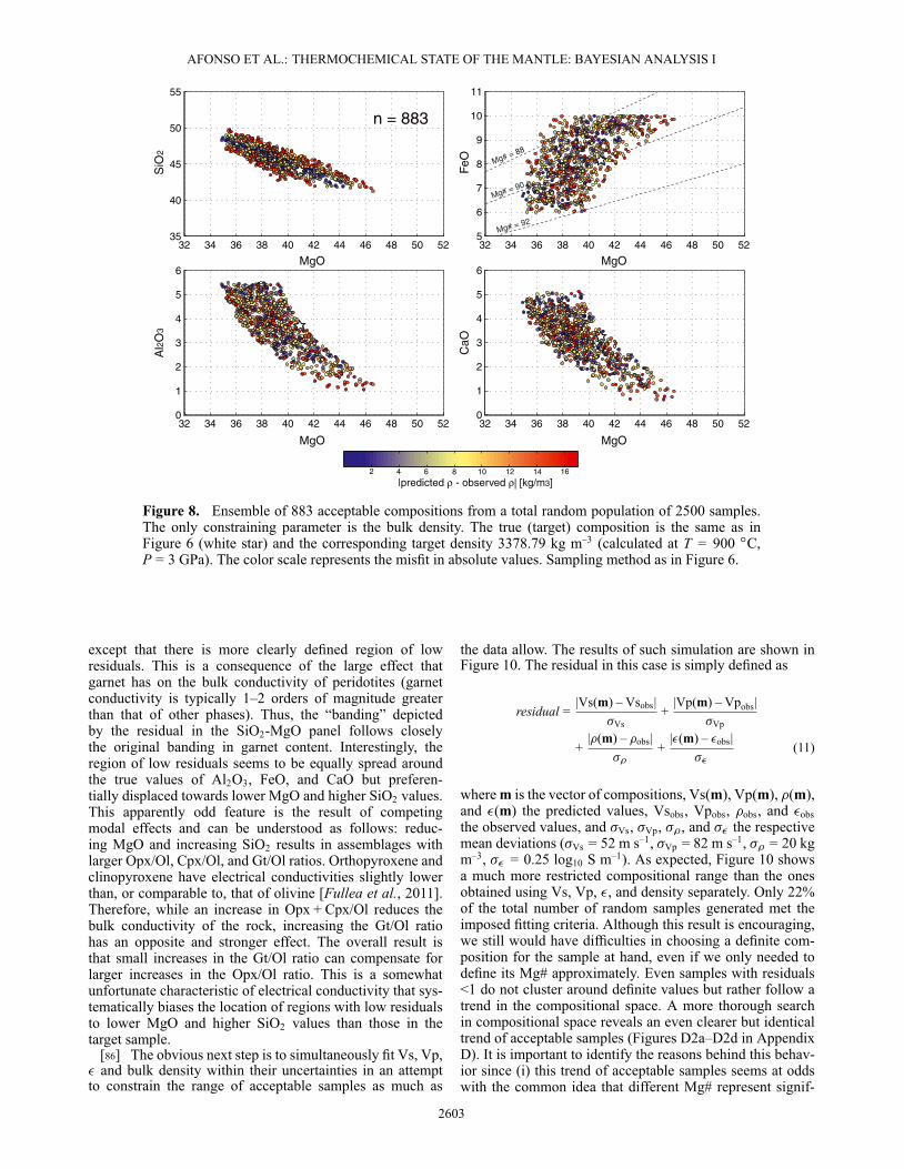
AFONSO ET AL.: THERMOCHEMICAL STATE OF THE MANTLE: BAYESIAN ANALYSIS I
32 34 36 38 40 42 44 46 48 50 5235
40
45
50
55
2 4 6 8 10 12 14 16
32 34 36 38 40 42 44 46 48 50 525
6
7
8
9
10
11
32 34 36 38 40 42 44 46 48 50 520
1
2
3
4
5
6
32 34 36 38 40 42 44 46 48 50 520
1
2
3
4
5
6MgOMgO
MgOMgO
CaO
Al2
O3
SiO
2
FeO
|predicted ρ - observed ρ| [kg/m3]
n = 883
Mg# = 88
Mg# = 90
Mg# = 92
Figure 8. Ensemble of 883 acceptable compositions from a total random population of 2500 samples.The only constraining parameter is the bulk density. The true (target) composition is the same as inFigure 6 (white star) and the corresponding target density 3378.79 kg m–3 (calculated at T = 900 ıC,P = 3 GPa). The color scale represents the misfit in absolute values. Sampling method as in Figure 6.
except that there is more clearly defined region of lowresiduals. This is a consequence of the large effect thatgarnet has on the bulk conductivity of peridotites (garnetconductivity is typically 1–2 orders of magnitude greaterthan that of other phases). Thus, the “banding” depictedby the residual in the SiO2-MgO panel follows closelythe original banding in garnet content. Interestingly, theregion of low residuals seems to be equally spread aroundthe true values of Al2O3, FeO, and CaO but preferen-tially displaced towards lower MgO and higher SiO2 values.This apparently odd feature is the result of competingmodal effects and can be understood as follows: reduc-ing MgO and increasing SiO2 results in assemblages withlarger Opx/Ol, Cpx/Ol, and Gt/Ol ratios. Orthopyroxene andclinopyroxene have electrical conductivities slightly lowerthan, or comparable to, that of olivine [Fullea et al., 2011].Therefore, while an increase in Opx + Cpx/Ol reduces thebulk conductivity of the rock, increasing the Gt/Ol ratiohas an opposite and stronger effect. The overall result isthat small increases in the Gt/Ol ratio can compensate forlarger increases in the Opx/Ol ratio. This is a somewhatunfortunate characteristic of electrical conductivity that sys-tematically biases the location of regions with low residualsto lower MgO and higher SiO2 values than those in thetarget sample.
[86] The obvious next step is to simultaneously fit Vs, Vp,� and bulk density within their uncertainties in an attemptto constrain the range of acceptable samples as much as
the data allow. The results of such simulation are shown inFigure 10. The residual in this case is simply defined as
residual =|Vs(m) – Vsobs|
�Vs+
|Vp(m) – Vpobs|�Vp
+|�(m) – �obs|
��+
|�(m) – �obs|��
(11)
where m is the vector of compositions, Vs(m), Vp(m), �(m),and �(m) the predicted values, Vsobs, Vpobs, �obs, and �obsthe observed values, and �Vs, �Vp, ��, and �� the respectivemean deviations (�Vs = 52 m s–1, �Vp = 82 m s–1, �� = 20 kgm–3, �� = 0.25 log10 S m–1). As expected, Figure 10 showsa much more restricted compositional range than the onesobtained using Vs, Vp, �, and density separately. Only 22%of the total number of random samples generated met theimposed fitting criteria. Although this result is encouraging,we still would have difficulties in choosing a definite com-position for the sample at hand, even if we only needed todefine its Mg# approximately. Even samples with residuals<1 do not cluster around definite values but rather follow atrend in the compositional space. A more thorough searchin compositional space reveals an even clearer but identicaltrend of acceptable samples (Figures D2a–D2d in AppendixD). It is important to identify the reasons behind this behav-ior since (i) this trend of acceptable samples seems at oddswith the common idea that different Mg# represent signif-
2603

AFONSO ET AL.: THERMOCHEMICAL STATE OF THE MANTLE: BAYESIAN ANALYSIS I
0.1 0.2 0.3 0.4 0.5
32 34 36 38 40 42 44 46 48 50 525
6
7
8
9
10
11
32 34 36 38 40 42 44 46 48 50 5235
40
45
50
55
32 34 36 38 40 42 44 46 48 50 520
1
2
3
4
5
6
32 34 36 38 40 42 44 46 48 50 520
1
2
3
4
5
6
MgO
MgO
MgO
MgO
|predicted log ε - observed log ε| [log S/m]
n = 2326
CaO
Al2
O3
SiO
2
FeO Mg# = 88
Mg# = 90
Mg# = 92
Gt
Figure 9. Ensemble of 2326 acceptable compositions from a total random population of 2500 sam-ples. The only constraining data is the bulk electrical conductivity. The true (target) composition isthe same as in Figure 6 (white star) and the corresponding target electrical conductivity is log10� = –3.9163
�log10 S m–1 (calculated at T = 900 ıC, P = 3 GPa). The black arrow indicates the direc-
tion of increasing garnet content in the samples. The color scale represents the misfit in absolute values.Sampling method as in Figure 6.
icantly different physical properties and (ii) it complicatesany inversion procedure within the compositional space.
[87] The trend of low misfit samples (blue dots), runningroughly from high-Mg/low-Al/high-Fe to low-Mg/high-Al/low-Fe, is the result of a combination of modal andcompositional effects. The high-Mg/low-Al/high-Fe sam-ples are basically harzburgites with anomalously high Aland Fe contents, while the low-Mg/high-Al/low-Fe samplesare lherzolites with anomalously low Fe contents (comparedwith natural samples in Figure 2). Over 95% of high-Mgperidotites in our database are depleted rocks with low con-tents of Al and Ca (Figure 2), which typically results inlow-density rocks with higher Vs and Vp velocities thantheir fertile counterparts. In the present case, however, theanomalously high FeO contents of the harzburgites pro-mote the stabilization of denser olivine (Fa-rich olivine)with lower Vp and Vs velocities than normal. Additionally,the relatively high Al contents of these samples result inhigher than normal contents of the dense phase garnet. Thefinal result is that the FeO and Al2O3 effects counterbal-ance the high-Mg effect, and thus the physical propertiesof the harzburgitic samples resemble those of more fertilelherzolites. This is the reason why the field of acceptablesamples is extended towards higher Mg# in Figure 10. Thecause of the extension towards lower Mg# can be understoodon similar grounds. The anomalously low FeO contentsin the lherzolitic samples of Figure 10 result in samples
with higher Vs and Vp and lower densities than averagenatural lherzolites (low-Fe end members are typically lessdense and have higher velocities). Importantly, note thatalthough the Al2O3 content is relatively high, this does nottranslate into significantly larger amounts of denser garnetdue to a “buffer” effect by the pyroxenes, which can accom-modate larger amounts of Al2O3 at low pressures [e.g.,Perkins and Newton, 1980]. This buffer effect is discussedfurther below.
[88] The existence of this trend complicates any attemptto constrain the composition of the sample, since all samplesare identical in terms of their relevant physical proper-ties (Table 2). This hitherto described problem representsa serious challenge for any inversion scheme attempting toprovide estimates of the compositional structure of the uppermantle. Interestingly, this modal-compositional effect is sig-nificantly minimized as the pressure increases, mainly due tothe disappearance of the buffer effect provided by pyroxenes(Appendix D). As mentioned above, the capacity of pyrox-enes to accommodate Al_2O_3 in their structure decreaseswith pressure [Perkins and Newton, 1980], which in turnamplifies the dependence of modal garnet on bulk Al2O3content. At the same time, the majoritic component of opxbecomes more soluble in garnet as pressure increases [e.g.,Irifune and Ringwood, 1993], thus increasing modal gt/opx.All this results in that even relatively small changes in Al2O3content at high pressures (P &10 GPa) can translate into
2604

AFONSO ET AL.: THERMOCHEMICAL STATE OF THE MANTLE: BAYESIAN ANALYSIS I
0.5 1 1.5 2 2.5
MgO
CaO
Al2
O3
SiO
2
FeO
MgO
MgO
MgO
combined residual (Eq. 11)
32 34 36 38 40 42 44 46 48 50 525
6
7
8
9
10
11
32 34 36 38 40 42 44 46 48 50 520
1
2
3
4
5
6
32 34 36 38 40 42 44 46 48 50 520
1
2
3
4
5
6
32 34 36 38 40 42 44 46 48 50 5235
40
45
50
55
n = 546
Mg# = 88
Mg# = 90
Mg# = 92
Figure 10. Ensemble of 546 acceptable compositions from a total random population of 2500 samples.These acceptable samples simultaneously fit Vs, Vp, electrical conductivity, and bulk density constraints(within uncertainties). True (target) composition and P-T conditions as in Figure 6, and the correspondingVp, Vs, �, and density as in Figures 6–9. The color scale represents the combined residual explained inthe text.
significant variations in the garnet mode. Since garnet is thedensest, fastest, and most conductive phase in the rock, mod-est variations in its mode significantly affect the physicalproperties of the rock. Because this modal effect is moreimportant than that exerted by modest variations in FeOcontent, the dependence of bulk density, Vs, Vp, and electricconductivity on compositional variations is effectively aug-mented at high pressures and thus the trend seen in Figure 10is much reduced (Appendix D). In summary, constrainingthe composition of an upper mantle peridotite using only its
physical properties is easier at depths &300 km. Thus, thedepth range over which constraining compositional anoma-lies with geophysical observables is less robust encompassesmost of the lithospheric mantle. Inversion schemes thatinclude a compositional space for the lithosphere shouldexplicitly consider this matter.4.3.2. A Simple Bayesian Strategy
[89] To this point, it would seem that the combinationof the four observations fails to define a good estimateof the sample’s composition, even when the experimental
Table 2. (a) Volumetric Proportions, Phase Compositions, and Physical Properties of a Peridotite Sample With Bulk Composition SiO2 =45.59, Al2O3 = 4.82, FeO = 7.0, MgO = 38.01, and CaO = 4.93. (b) Volumetric Proportions, Phase Compositions, and Physical Propertiesof a Peridotite Sample With Bulk Composition SiO2 = 42.27, Al2O3 = 2.50, FeO = 9.84, MgO = 45.00, and CaO = 0.57a
(a) Phases vol% SiO2 Al2O3 FeO MgO CaO � [kg m–3] Vs [km s–1] Vp [km s–1]
Ol 54.65 41.81 0.00 8.13 50.68 0.00 3324.0 4.65 8.20Opx 10.65 57.50 0.95 6.45 34.59 0.51 3300.3 4.53 7.73Cpx 17.26 54.82 0.89 1.36 18.36 24.57 3296.3 4.36 7.76Gt 17.43 42.52 23.95 8.96 20.76 3.81 3688.5 4.94 8.89Aggregate x 45.59 4.82 7.0 38.01 4.93 3380.2 4.63 8.18
(b) Phases vol% SiO2 Al2O3 FeO MgO CaO � [kg m–3] Vs [km s–1] Vp [km s–1]
Ol 83.04 40.83 0.00 9.99 49.17 0.00 3348.3 4.61 8.15Opx 7.11 57.26 0.89 7.49 33.87 0.47 3313.3 4.51 7.70Cpx 0.55 54.74 0.88 1.65 18.12 24.59 3299.9 4.36 7.76Gt 9.30 42.21 23.77 10.47 19.59 3.95 3711.8 4.93 8.86Aggregate x 42.27 2.50 9.84 45.00 0.57 3379.3 4.63 8.18
aCalculations were performed with Perple_X [Connolly, 2009] at P = 3 GPa, T = 900 ıC. The thermodynamic formalism and database are from Stixrudeand Lithgow-Bertelloni [2011].
2605
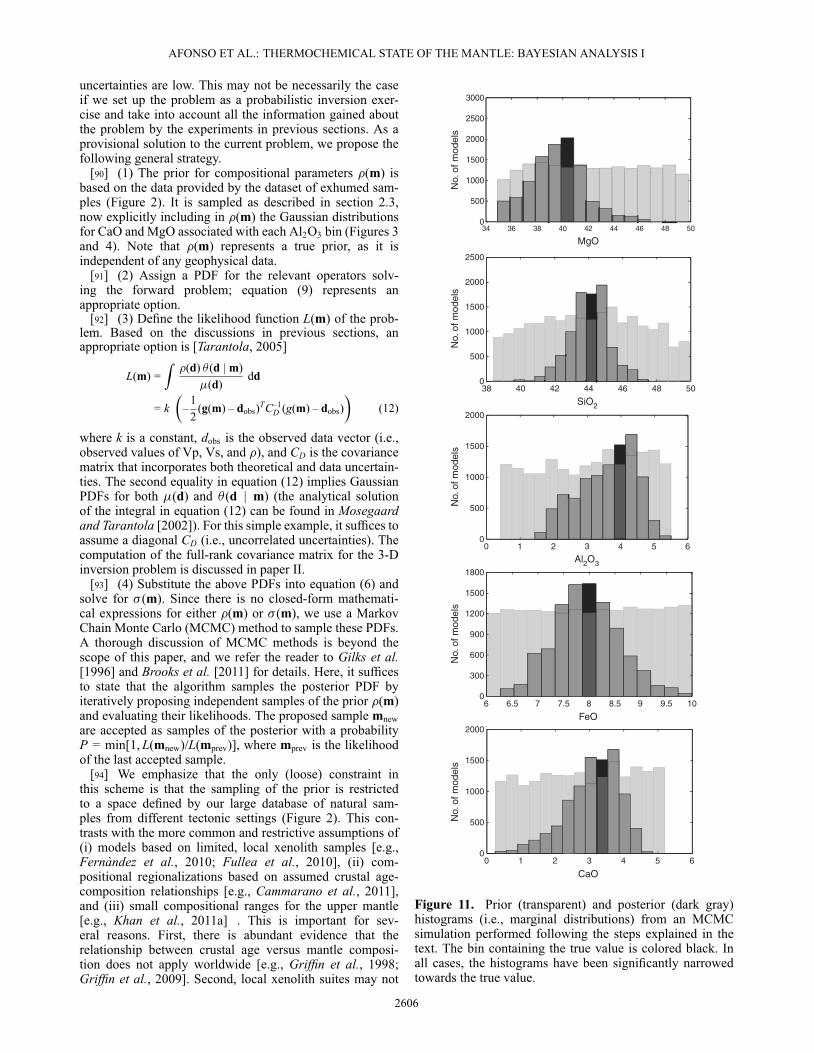
AFONSO ET AL.: THERMOCHEMICAL STATE OF THE MANTLE: BAYESIAN ANALYSIS I
uncertainties are low. This may not be necessarily the caseif we set up the problem as a probabilistic inversion exer-cise and take into account all the information gained aboutthe problem by the experiments in previous sections. As aprovisional solution to the current problem, we propose thefollowing general strategy.
[90] (1) The prior for compositional parameters �(m) isbased on the data provided by the dataset of exhumed sam-ples (Figure 2). It is sampled as described in section 2.3,now explicitly including in �(m) the Gaussian distributionsfor CaO and MgO associated with each Al2O3 bin (Figures 3and 4). Note that �(m) represents a true prior, as it isindependent of any geophysical data.
[91] (2) Assign a PDF for the relevant operators solv-ing the forward problem; equation (9) represents anappropriate option.
[92] (3) Define the likelihood function L(m) of the prob-lem. Based on the discussions in previous sections, anappropriate option is [Tarantola, 2005]
L(m) =Z�(d) � (d | m)
�(d)dd
= k�
–12
(g(m) – dobs)TC–1D (g(m) – dobs)
�(12)
where k is a constant, dobs is the observed data vector (i.e.,observed values of Vp, Vs, and �), and CD is the covariancematrix that incorporates both theoretical and data uncertain-ties. The second equality in equation (12) implies GaussianPDFs for both �(d) and � (d | m) (the analytical solutionof the integral in equation (12) can be found in Mosegaardand Tarantola [2002]). For this simple example, it suffices toassume a diagonal CD (i.e., uncorrelated uncertainties). Thecomputation of the full-rank covariance matrix for the 3-Dinversion problem is discussed in paper II.
[93] (4) Substitute the above PDFs into equation (6) andsolve for � (m). Since there is no closed-form mathemati-cal expressions for either �(m) or � (m), we use a MarkovChain Monte Carlo (MCMC) method to sample these PDFs.A thorough discussion of MCMC methods is beyond thescope of this paper, and we refer the reader to Gilks et al.[1996] and Brooks et al. [2011] for details. Here, it sufficesto state that the algorithm samples the posterior PDF byiteratively proposing independent samples of the prior �(m)and evaluating their likelihoods. The proposed sample mneware accepted as samples of the posterior with a probabilityP = min[1, L(mnew)/L(mprev)], where mprev is the likelihoodof the last accepted sample.
[94] We emphasize that the only (loose) constraint inthis scheme is that the sampling of the prior is restrictedto a space defined by our large database of natural sam-ples from different tectonic settings (Figure 2). This con-trasts with the more common and restrictive assumptions of(i) models based on limited, local xenolith samples [e.g.,Fernàndez et al., 2010; Fullea et al., 2010], (ii) com-positional regionalizations based on assumed crustal age-composition relationships [e.g., Cammarano et al., 2011],and (iii) small compositional ranges for the upper mantle[e.g., Khan et al., 2011a] . This is important for sev-eral reasons. First, there is abundant evidence that therelationship between crustal age versus mantle composi-tion does not apply worldwide [e.g., Griffin et al., 1998;Griffin et al., 2009]. Second, local xenolith suites may not
38 40 42 44 46 48 500
500
1000
1500
2000
2500
6 6.5 7 7.5 8 8.5 9 9.5 100
300
600
900
1200
1500
1800
0 1 2 3 4 5 60
500
1000
1500
2000
0 1 2 3 4 5 60
500
1000
1500
2000
No.
of m
odel
sN
o. o
f mod
els
No.
of m
odel
sN
o. o
f mod
els
34 36 38 40 42 44 46 48 500
500
1000
1500
2000
2500
3000
No.
of m
odel
s
MgO
SiO2
Al2O3
FeO
CaO
Figure 11. Prior (transparent) and posterior (dark gray)histograms (i.e., marginal distributions) from an MCMCsimulation performed following the steps explained in thetext. The bin containing the true value is colored black. Inall cases, the histograms have been significantly narrowedtowards the true value.
2606
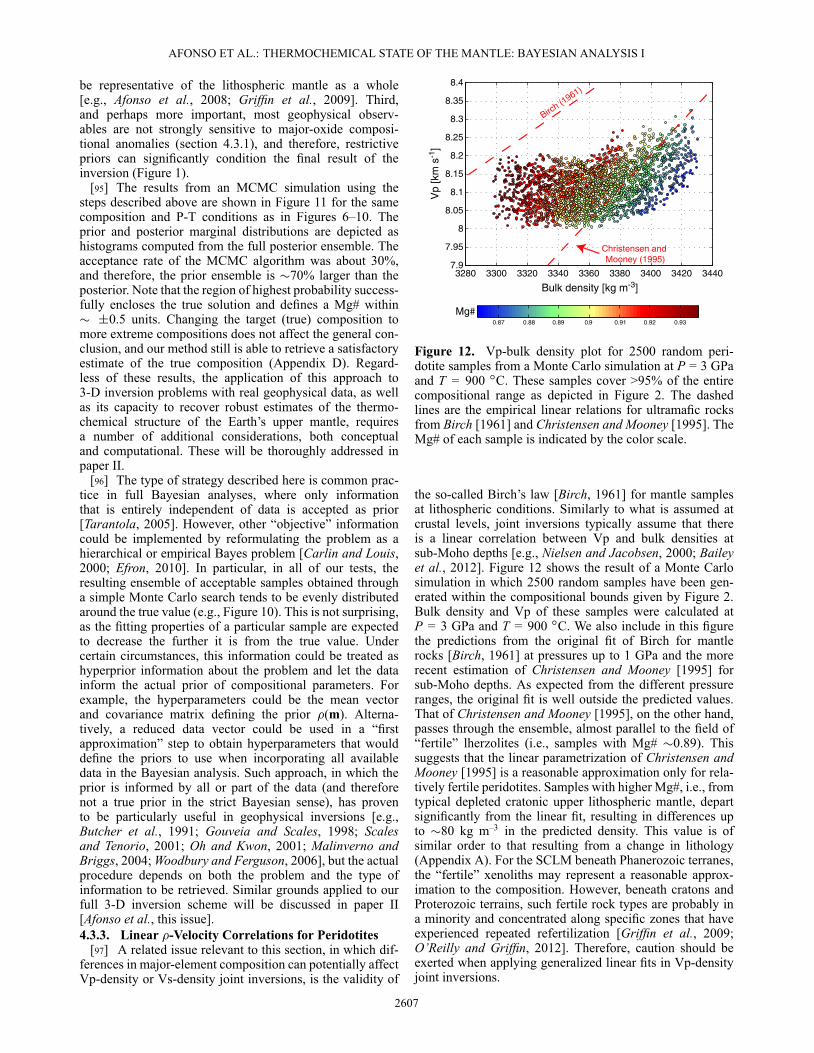
AFONSO ET AL.: THERMOCHEMICAL STATE OF THE MANTLE: BAYESIAN ANALYSIS I
be representative of the lithospheric mantle as a whole[e.g., Afonso et al., 2008; Griffin et al., 2009]. Third,and perhaps more important, most geophysical observ-ables are not strongly sensitive to major-oxide composi-tional anomalies (section 4.3.1), and therefore, restrictivepriors can significantly condition the final result of theinversion (Figure 1).
[95] The results from an MCMC simulation using thesteps described above are shown in Figure 11 for the samecomposition and P-T conditions as in Figures 6–10. Theprior and posterior marginal distributions are depicted ashistograms computed from the full posterior ensemble. Theacceptance rate of the MCMC algorithm was about 30%,and therefore, the prior ensemble is �70% larger than theposterior. Note that the region of highest probability success-fully encloses the true solution and defines a Mg# within� ˙0.5 units. Changing the target (true) composition tomore extreme compositions does not affect the general con-clusion, and our method still is able to retrieve a satisfactoryestimate of the true composition (Appendix D). Regard-less of these results, the application of this approach to3-D inversion problems with real geophysical data, as wellas its capacity to recover robust estimates of the thermo-chemical structure of the Earth’s upper mantle, requiresa number of additional considerations, both conceptualand computational. These will be thoroughly addressed inpaper II.
[96] The type of strategy described here is common prac-tice in full Bayesian analyses, where only informationthat is entirely independent of data is accepted as prior[Tarantola, 2005]. However, other “objective” informationcould be implemented by reformulating the problem as ahierarchical or empirical Bayes problem [Carlin and Louis,2000; Efron, 2010]. In particular, in all of our tests, theresulting ensemble of acceptable samples obtained througha simple Monte Carlo search tends to be evenly distributedaround the true value (e.g., Figure 10). This is not surprising,as the fitting properties of a particular sample are expectedto decrease the further it is from the true value. Undercertain circumstances, this information could be treated ashyperprior information about the problem and let the datainform the actual prior of compositional parameters. Forexample, the hyperparameters could be the mean vectorand covariance matrix defining the prior �(m). Alterna-tively, a reduced data vector could be used in a “firstapproximation” step to obtain hyperparameters that woulddefine the priors to use when incorporating all availabledata in the Bayesian analysis. Such approach, in which theprior is informed by all or part of the data (and thereforenot a true prior in the strict Bayesian sense), has provento be particularly useful in geophysical inversions [e.g.,Butcher et al., 1991; Gouveia and Scales, 1998; Scalesand Tenorio, 2001; Oh and Kwon, 2001; Malinverno andBriggs, 2004; Woodbury and Ferguson, 2006], but the actualprocedure depends on both the problem and the type ofinformation to be retrieved. Similar grounds applied to ourfull 3-D inversion scheme will be discussed in paper II[Afonso et al., this issue].4.3.3. Linear �-Velocity Correlations for Peridotites
[97] A related issue relevant to this section, in which dif-ferences in major-element composition can potentially affectVp-density or Vs-density joint inversions, is the validity of
3280 3300 3320 3340 3360 3380 3400 3420 34407.9
7.95
8
8.05
8.1
8.15
8.2
8.25
8.3
8.35
8.4
0.87 0.88 0.89 0.9 0.91 0.92 0.93
Vp
[km
s-1
]
Bulk density [kg m-3]
Mg#
Birch (1
961)
Christensen and Mooney (1995)
Figure 12. Vp-bulk density plot for 2500 random peri-dotite samples from a Monte Carlo simulation at P = 3 GPaand T = 900 ıC. These samples cover >95% of the entirecompositional range as depicted in Figure 2. The dashedlines are the empirical linear relations for ultramafic rocksfrom Birch [1961] and Christensen and Mooney [1995]. TheMg# of each sample is indicated by the color scale.
the so-called Birch’s law [Birch, 1961] for mantle samplesat lithospheric conditions. Similarly to what is assumed atcrustal levels, joint inversions typically assume that thereis a linear correlation between Vp and bulk densities atsub-Moho depths [e.g., Nielsen and Jacobsen, 2000; Baileyet al., 2012]. Figure 12 shows the result of a Monte Carlosimulation in which 2500 random samples have been gen-erated within the compositional bounds given by Figure 2.Bulk density and Vp of these samples were calculated atP = 3 GPa and T = 900 ıC. We also include in this figurethe predictions from the original fit of Birch for mantlerocks [Birch, 1961] at pressures up to 1 GPa and the morerecent estimation of Christensen and Mooney [1995] forsub-Moho depths. As expected from the different pressureranges, the original fit is well outside the predicted values.That of Christensen and Mooney [1995], on the other hand,passes through the ensemble, almost parallel to the field of“fertile” lherzolites (i.e., samples with Mg# �0.89). Thissuggests that the linear parametrization of Christensen andMooney [1995] is a reasonable approximation only for rela-tively fertile peridotites. Samples with higher Mg#, i.e., fromtypical depleted cratonic upper lithospheric mantle, departsignificantly from the linear fit, resulting in differences upto �80 kg m–3 in the predicted density. This value is ofsimilar order to that resulting from a change in lithology(Appendix A). For the SCLM beneath Phanerozoic terranes,the “fertile” xenoliths may represent a reasonable approx-imation to the composition. However, beneath cratons andProterozoic terrains, such fertile rock types are probably ina minority and concentrated along specific zones that haveexperienced repeated refertilization [Griffin et al., 2009;O’Reilly and Griffin, 2012]. Therefore, caution should beexerted when applying generalized linear fits in Vp-densityjoint inversions.
2607

AFONSO ET AL.: THERMOCHEMICAL STATE OF THE MANTLE: BAYESIAN ANALYSIS I
700 800 900 1000 11000
100
200
300
400F
requ
ency
Temperature [0C]
n = 990
92% of the total
700 800 900 1000 11000
800
200
600
400
Fre
quen
cy
n = 2326
a
b86% of the total
1.51 1.32 1.201.61
0.682.08 2.21
high
er p
oste
rior
PD
F
Figure 13. Histogram of 990 samples that fit Vp, Vs,bulk density, and electrical conductivity within uncertain-ties. Note that more than 92% of these samples are foundwithin the range 800 < T < 1000ıC. (b) as in (a) but exclud-ing electrical conductivity from the constraining parameters.The color scale denotes values of the normalized poste-rior PDF. Numbers between two temperature bins are theaverage residuals (as defined in equation (11)) for the twoadjacent bins. See text for details.
4.4. Dependence of Physical Parameterson Temperature
[98] The effect of temperature on anharmonic physi-cal properties of upper mantle minerals is generally betterunderstood than the compositional effects [cf. Ahrens, 1995,Anderson, 1995; Rubie et al., 2004; Yoshino, 2010;Price, 2009; Jones et al., 2012]. Therefore, we do notattempt to address this subject here; the interested reader canfind detailed reviews in the references given above. Morerelevant to us is the minimum range of temperatures thatour observables can constrain when compositional effectsare simultaneously included in the inversion. In Bayesianterms, we would like to know how broad the likelihoodfunction is (and therefore the posterior PDF) with respectto temperature. An instructive and simple way to achievethis is to add temperature to our vector of model parame-ters m and run Monte Carlo simulations to find acceptableensembles that fit the data within uncertainties. The strategyhere is first to generate 2500 random compositional sam-ples in the same way as in the previous section and then tocalculate their physical properties for 40 different tempera-ture bins of 25ıC each. This provides a sufficiently smoothsampling of temperature from 500 to 1500ıC (note that thetarget sample still is at T = 900 ıC). Thus, the total num-ber of random samples generated in this example amountsto 100,000.
[99] The results of this simulation for two cases, oneincluding electrical conductivity as a constraint and theother neglecting it, are shown in Figure 13. When theconstraining parameters include the electrical conductivity,the total number of acceptable samples is 990, which rep-resents �1% of the total number of generated samples.In this case, more than 90% of the samples comprisingthe acceptable ensemble are restricted to a temperaturerange of 200ıC (Figure 13a), and more than 62% lieswithin a range of 100ıC. Removing the electrical con-ductivity from the constraining parameters (i.e., Vp, Vs,and density only) results in an acceptable ensemble con-taining 2326 samples, �2.36% of the original samples.Approximately 90% of the ensemble now lies within atemperature range of 250ıC (Figure 13b), which reflectsthe fact that the electrical conductivity of solid assem-blages is much more sensitive to temperature changes thanthe other three parameters. While electrical conductivityis exponentially dependent on temperature (equation (8))[Jones et al., 2009; Fullea et al., 2011], Vp, Vs, and den-sity exhibit a quasi-linear or weakly nonlinear dependence(i.e., for most mantle phases the first temperature derivativeis dominant) [see Jones et al., 2009; Afonso et al., 2010, andreferences therein].
[100] The reason for obtaining larger acceptable ensem-bles when temperature is included as a free parameter istwofold. First, small changes in the temperature (i.e., fromone temperature bin to another) are likely to translate intosmall changes of the physical parameters, which in turn arelikely to remain within the assigned experimental uncer-tainties. For instance, a change from 500 to 525ıC resultsin changes of –2.51 kg m–3, –0.008 km s–1, and –0.014km s–1 in density, Vs, and Vp, respectively. These varia-tions are much smaller than the experimental uncertaintiesassigned to each variable (see previous section). The sec-ond factor is the well-known trade-off between temperatureand composition for some parameters [e.g., seismic veloci-ties) [Afonso et al., 2010], which has the potential to convertunacceptable samples at one temperature into acceptablesamples at another temperature. This is particularly evi-dent in Figure 13b, where larger numbers of acceptablesamples are found at temperatures lower than the truevalue. In this case, most of the samples with low FeOand low MgO, characterized by low relative densities andrejected in Figure 10, become acceptable at lower tempera-tures (i.e., they compensate their low compositional densitywith temperature). Since electrical conductivity constrainstemperature better, this effect is diminished in Figure 13a(albeit still visible).
[101] If we were to adopt a frequentist point of view, itwould be tempting to assign 875 and 825ıC as the mostlikely temperatures in these ensembles. However, using thedefinition in item 4 in section 4.3.3 for the posterior PDFand an MCMC simulation, the most likely temperature islocated within the range 875 < T < 925ıC in both cases.This is depicted in Figure 13 by superimposing a colorscale of the resulting marginal posterior on top of the MonteCarlo histograms. We emphasize that the histograms repre-sent the number of samples that are compatible with datawithin uncertainties (frequentist analysis), while the colorscale is the result of a full MCMC simulation (Bayesiananalysis) with a flat prior in the temperature range 500 < T
2608

AFONSO ET AL.: THERMOCHEMICAL STATE OF THE MANTLE: BAYESIAN ANALYSIS I
< 1500ıC. Although the marginal posterior for temperatureis narrower in the case which includes electrical conductiv-ity, the marginals for compositional parameters are slightlydeteriorated in comparison to the case with Vs, Vp, and den-sity only. This seems to be an unavoidable consequence ofthe intrinsic dependence of electrical conductivity on modalgarnet and bulk MgO content (section 4.3.1). The additionof fluids and/or carbon-rich phases to the system would addanother layer of complexity to the simultaneous treatmentof Vs, Vp, density, and electrical conductivity. However, wedeem that the results in this paper warrant a more compre-hensive exploration of the potential benefits (temperature?)and limitations (composition?) of incorporating electricalconductivity in multiobservable inversions.
5. Conclusion[102] In this paper, we have analyzed the main problems
associated with the definitions and use of a priori infor-mation on compositional parameters �(m) and likelihoodfunction L(m) for probabilistic inversion schemes aimed toconstrain the thermochemical structure of the Earth’s litho-sphere and sublithospheric upper mantle. Within this con-text, the need for combining multiple geophysical datasetsin a probabilistic manner has been justified and demon-strated by analyzing the sensitivity of each observable tocomposition and temperature, as well as their experimentaluncertainties. The dependence of physical parameters suchas bulk density, electrical conductivity, and seismic veloci-ties to major-element composition has been systematicallyaddressed using Monte Carlo simulations and an internallyconsistent thermodynamic formalism.
[103] Based on this analysis, we propose a generalstrategy to define �(m) that does not rely on restrictiveassumptions such as small ad hoc compositional ranges,limited/local xenolith populations, or predefined �(m) forspecific tectonic settings based on age-composition rela-tionships. This is important as there is ample evidenceof exceptions to such age-composition relationships; theseexceptions carry significant tectonic information and arethus one of the targets to be identified by the presentapproach. The problem of using age-composition rela-tionships as a priori information is aggravated by thefact that the likelihood, which should account for realis-tic uncertainties in data and theory, is only mildly sen-sitive to bulk compositional parameters. We have shownthe intrinsic difficulties in obtaining reliable compositionalestimates of peridotite samples when using geophysicalparameters/observables. Most importantly, by using simplesynthetic examples, we have shown that a wide range ofnaturally occurring compositions can equally well explainmultiple geophysical data. This nonuniqueness problem isheightened at lithospheric depths, where most of the com-positional variability is expected to occur, and thus, it rep-resents a major challenge not only for traditional linearizedinversions but also for explorative Monte Carlo methods.Any method attempting to estimate the compositional andthermal structure of the upper mantle should address theseproblems.
[104] In this first paper, we have demonstrated that amultiobservable Bayesian approach, in which the a prioriinformation is based on large databases of natural mantle
samples and robust correlations between major oxides offera promising and general inference platform to address theabovementioned difficulties. The two key elements of themethod are (i) the internally consistent combination of mul-tiple geophysical observables with differential sensitivitiesto compositional/thermal parameters and (ii) a priori com-positional information based on statistical analysis of largedatabases of natural mantle samples from many differenttectonic settings. This database can be updated as more sam-ples are analyzed, without affecting the general inversionscheme. We have shown that such approach can provideacceptable (probabilistic) estimates of both compositionalvariables and associated uncertainties. Nevertheless, theapplication of this probabilistic approach to 3-D inversionscenarios requires additional considerations at both techni-cal and conceptual levels. We address these in detail in anaccompanying paper [Afonso et al., paper II, this issue].
Appendix A: Eclogites and Pyroxenites[105] Eclogitic and pyroxenitic xenoliths are commonly
recovered in both cratonic and off-craton localities aroundthe world [Schulze, 1989; Jacob, 2004; Griffin and O’Reilly,2007]. Although in most these two lithologies are subordi-nate in comparison to peridotite xenoliths, some localitiesexhibit a clear dominance of eclogites/pyroxenites in theirxenolith population (e.g., Roberts Victor, South Africa).However, even in such cases, the relatively large abun-dance of eclogites is thought to be the result of eitherdifferential preservation effects during xenolith exhumationor sampling-depth bias [Jacob, 2004; Griffin and O’Reilly,2007]. In fact, although their origin and role in the evolu-tion of lithospheric mantle still are a matter of debate [Griffinand O’Reilly, 2007], it is commonly accepted that eclogitesand pyroxenites cannot make up more than �1% in vol-ume of the lithospheric mantle [Schulze, 1989], althoughhigher local concentrations could exist [e.g., Griffin andO’Reilly, 2007; Huang et al., 2012]. Since our method isdesigned to capture average compositional heterogeneitiesin the mantle with minimum vertical and horizontal exten-sions &40 and 80 km, respectively (Afonso et al., paper II,this volume), it is not suited for detecting sharp lithologicalcontrasts or volumetrically unimportant bodies.
[106] Although beyond the scope of this paper, we notethat detection of eclogitic bodies in the mantle by othergeophysical techniques is also difficult task [e.g., Ghentet al., 2004; Bascou et al., 2001], particularly becausenot all eclogites are characterized by significantly dif-ferent physical properties from those of peridotites. Forinstance, Figure A1 shows the Vs, Vp, and bulk densityof 2500 randomly generated eclogitic samples based onthe xenolith database of Huang et al. [2012]. The latter isdepicted in the figure as histograms indicating the relativeabundance of eclogitic xenoliths in terms of their Al2O3and FeO contents. This figure also includes the Vp, Vs,and density of typical mantle peridotites at the same P-T conditions (red shaded rectangles). Except for density,which is always lower in peridotites, Vp and Vs of man-tle peridotites lie within the compositional range observedin eclogitic xenoliths. More importantly, the compositionalregion at which the two lithologies have similar seismicvelocities coincides with that of the most abundant eclogitic
2609

AFONSO ET AL.: THERMOCHEMICAL STATE OF THE MANTLE: BAYESIAN ANALYSIS I
8 10 12 14 16 18 207.9
88.18.28.38.48.58.68.78.8
8 10 12 14 16 18 203350
3400
3450
3500
3550
3600
3650
3700
3750
4 6 8 10 12 14 163350
3400
3450
3500
3550
3600
3650
3700
3750
8 10 12 14 16 18 204.4
4.5
4.6
4.7
4.8
4.9
5
6
8
10
12
14
6
8
10
12
14
6
8
10
12
14
10
12
14
16
18
FeO
FeO
FeO
MgO
Al2O3 FeO
Den
sity
[kg/
m3 ]
Den
sity
[kg/
m3 ]
Vs
[km
/s]
Vp
[km
/s]
Al2O3 Al2O3
Figure A1. The figure shows the main physical parameters for 2500 random samples generated basedon the database of Huang et al. [2012]. Color scale as in Figure 2. The histograms indicate the frequencyof samples in the database. Shaded red bands denote typical values for mantle peridotite at identical P-Tconditions.
xenoliths (i.e., the isotropic seismic velocities of the mostcommonly sampled eclogites are not too different from thoseof surrounding peridotites). In particular, none of the sam-ples plotted in Figure A1 produces reflectivity coefficients>0.07, in agreement with previous studies [e.g., Bascouet al., 2001; Ji et al., 2003b]. This corroborates previoussuggestions that the simple contrast in physical propertiesbetween peridotite and eclogite is insufficient to produce thehigh-amplitude reflections inferred in some localities [e.g.,Bascou et al., 2001; Morgan et al., 2000; Ji et al., 2003b].However, interlayered heterogeneities (e.g., vertical layeringof peridotite-eclogite) with the proper thickness could pro-duce local constructive interference and high reflectivity.
Appendix B: Na-CFMAS and H2O-CFMASVersus CFMAS
[107] The addition of Na2O to the CFMAS systemrequires additional end members and more elaborated solid-solution models than in the simpler CFMAS system. Thistranslates into much longer computation times in the energyminimization problem, and thus, the performance of theinversion scheme is deteriorated. Therefore, the followingquestion arises: does the inclusion of Na2O into the CFMASsystem improve the result of the inversion scheme to a sig-nificant extent? In order to answer this question, we have runa number of Monte Carlo simulations at different P-T con-ditions and for different compositions. Figure B1 shows theresults of one of such simulations for identical P-T-C condi-tions as those used to obtain Figure 11. A visual comparisonof these figures suggest that the recovered fields of high a
posteriori probability (solution to the inverse problem) withand without Na2O are almost identical. Similar results wereobtained for other peridotite compositions and P-T condi-tions. Based on these results, and considering the modestsensitivity of geophysical observables to bulk composition,we conclude that there is no practical justification for, orobvious advantage in, including Na2O in our inversion. Wenote, however, that this is strictly valid if the assumption ofan upper mantle dominated by peridotite holds true. If largeamounts of basaltic or eclogitic material (>20 vol% of “nor-mal” mantle) are present as mechanically and chemicallyindependent lithologies, the need to consider Na2O in thecomputation could be justified [e.g., Xu et al., 2008]. Morework towards subjecting the “mixture hypothesis” to a rig-orous probabilistic test (using geophysical observables) andgeochemical/petrological arguments will be needed.
[108] The addition of water to the system implies a sub-stantial increase in the number of phases (e.g., micas andamphiboles) and solution models that need to be consid-ered during the minimization problem. The computationtime necessary to solve one minimization problem withinthe H2O-CFMAS can be as large as fivefold or more com-pared to the dry counterpart. We have explored the effectsof including H2O in our computations by using a modified-augmented version of Holland and Powell’s [1998] ther-modynamic database as described in Connolly and Kerrick[2002] and Afonso and Zlotnik [2011]. We found that, asan approximate rule-of-thumb, for every 1 wt% increasein H2O, there is a decrease of 1% and 2% in the anhar-monic Vs and bulk density of peridotites, respectively, dueto the appearance of “soft” hydrous minerals. This is con-sistent with other previous estimations [e.g., Carlson and
2610

AFONSO ET AL.: THERMOCHEMICAL STATE OF THE MANTLE: BAYESIAN ANALYSIS I
38 40 42 44 46 48 500
500
1000
1500
2000
2500
6 6.5 7 7.5 8 8.5 9 9.5 100
300
600
900
1200
1500
1800
0 1 2 3 4 5 60
500
1000
1500
2000
0 1 2 3 4 5 60
500
1000
1500
2000
No.
of m
odel
sN
o. o
f mod
els
No.
of m
odel
sN
o. o
f mod
els
34 36 38 40 42 44 46 48 500
500
1000
1500
2000
2500
3000
No.
of m
odel
s
MgO
SiO2
Al2O3
FeO
CaO
Figure B1. Results from an MCMC simulation using thesame target composition and P-T conditions as in Figure 11,but including Na2O in the energy minimization problem.The thermodynamic database and formalism are those ofStixrude and Lithgow-Bertelloni [2011].
Miller, 2003]. Since the typical water content in SCLMrocks is <400 ppm, or �0.04 wt%, the expected anhar-monic Vs and density reductions are �0.04% and 0.08%,respectively. Even in localized areas of volatile-rich peri-dotites (e.g., metasomatized veins/conduits) with averagewater contents twice or three times as high, the associateddecrease in Vs and density is not expected reach 0.1% and0.2%, respectively. Therefore, variations in water content ofthe order of a few hundreds ppm can be ignored when deal-ing with seismic and/or gravity data (except, of course, insubduction zone environments). Electrical conductivity, onthe other hand, is much more sensitive to small variationsin water content in mantle rocks, and in principle, it couldbe used to infer water contents that other observables cannotdetect [Jones et al., 2012]. The difficulty is that the necessaryexperimental information on the effects that water has on theconductivity of mantle minerals at upper mantle conditionsstill is subject to debate [see discussion in Jones et al., 2012].Also, water-assisted attenuation effects on nominally anhy-drous phases [Karato, 2012, and references therein] has notbeen included in this study due to the lack of robust quan-titative models. However, due to the low water content inSCLM rocks, this effect also would be negligible. Althougha thorough exploration of the possibility of mapping “wateranomalies” is beyond the scope of this paper, we notethat our method is perfectly suitable to accommodatesuch possibility.
Appendix C: Gravity and Geoid Sensitivities toShallow/Deep Density Structures
[109] Geoid anomalies are more sensitive to deep den-sity variations than gravity anomalies, and therefore, theyrepresent an important constraint in lithospheric modeling.Figure C1 shows a synthetic model with two topographicheights, one is compensated purely by crustal isostasy andthe other purely by thermal (lithospheric) isostasy. The dif-ference between these two heights in terms of the Bougueranomaly is only <18 mGals. Such low values could eas-ily be masked by small density variations at shallow lev-els and therefore, it would be difficult to identify thethinning in the lithosphere. The geoid anomaly, on theother hand, exhibits a difference of >8 m. This valuewould be difficult to explain by shallow density anomaliesonly, particularly because the magnitude of the anomaliesrequired to explain the geoid would seriously perturb thepredicted topography.
Appendix D: Different Compositions and PTConditions
[110] The Bayesian strategy described in the text has beenjustified by the results it predicts, but results for only onecomposition at specific P-T conditions were shown. Here,we show the method still is able to retrieve a robust estimateof the true composition when the target composition or theP-T conditions are changed.
[111] Figure D1 shows the results from an MCMC sim-ulation using the steps described in the text for a different,more depleted, composition (SiO2 = 44.04, Al2O3 = 1.26,FeO = 6.52, MgO = 46.95, and CaO = 1.21). Note that the
2611
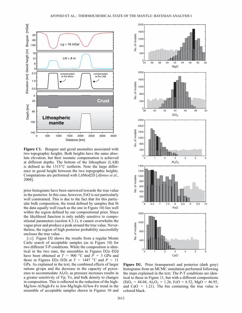
AFONSO ET AL.: THERMOCHEMICAL STATE OF THE MANTLE: BAYESIAN ANALYSIS I
Lithosphericmantle
Crust
2.0
1.0
0.0
-100
-60
-20
g < 18 mGal
compensatedat the LAB
compensatedat the Moho
Ele
vatio
n [k
m]
Geo
id h
eigt
h [m
]B
ougu
er [
mG
al]
Dep
th [k
m]
Distance [km]
N > 8 m
0
6
12
18
Figure C1. Bouguer and geoid anomalies associated withtwo topographic heights. Both heights have the same abso-lute elevation, but their isostatic compensation is achievedat different depths. The bottom of the lithosphere (LAB)is defined as the 1315ıC isotherm. Note the large differ-ence in geoid height between the two topographic heights.Computations are performed with LitMod2D [Afonso et al.,2008].
prior histograms have been narrowed towards the true valuein the posterior. In this case, however, FeO is not particularlywell constrained. This is due to the fact that for this partic-ular bulk composition, the trend defined by samples that fitthe data equally well (such as the one in Figure 10) lies wellwithin the region defined by our compositional prior. Sincethe likelihood function is only mildly sensitive to compo-sitional parameters (section 4.3.1), it cannot overwhelm thevague prior and produce a peak around the true value. Never-theless, the region of high posterior probability successfullyencloses the true value.
[112] Figure D2 shows the results from a regular MonteCarlo search of acceptable samples (as in Figure 10) fortwo different T-P conditions. While the composition is iden-tical in the two runs, the ensembles in Figures D2a–D2dhave been obtained at T = 900 ıC and P = 3 GPa andthose in Figures D2e–D2h at T = 1447 ıC and P = 11GPa. As explained in the text, the combined effects of largerrations gt/opx and the decrease in the capacity of pyrox-enes to accommodate Al2O3 as pressure increases results ina greater sensitivity of Vp, Vs, and bulk density to changesin composition. This is reflected in the reduction of the high-Mg/low-Al/high-Fe to low-Mg/high-Al/low-Fe trend in theensemble of acceptable samples shown in Figures 10 and
MgO
SiO2
Al2O3
FeO
CaO
34 36 38 40 42 44 46 48 500
400
800
1200
1600
2000
6 6.5 7 7.5 8 8.5 9 9.5 100
200
400
600
800
1000
1200
1400
0 1 2 3 4 5 60
400
800
1200
1600
2000
2400
0 1 2 3 4 5 60
400
800
1200
1600
38 40 42 44 46 48 500
400
800
1200
1600
2000
No.
of m
odel
sN
o. o
f mod
els
No.
of m
odel
sN
o. o
f mod
els
No.
of m
odel
s
Figure D1. Prior (transparent) and posterior (dark gray)histograms from an MCMC simulation performed followingthe steps explained in the text. The P-T conditions are iden-tical to those in Figure 11, but with a different compositions(SiO2 = 44.04, Al2O3 = 1.26, FeO = 6.52, MgO = 46.95,and CaO = 1.21). The bin containing the true value iscolored black.
2612

AFONSO ET AL.: THERMOCHEMICAL STATE OF THE MANTLE: BAYESIAN ANALYSIS I
32 34 36 38 40 42 44 46 48 50 5235
40
45
50
55
32 34 36 38 40 42 44 46 48 50 525
6
7
8
9
10
11
32 34 36 38 40 42 44 46 48 50 520
1
2
3
4
5
6
32 34 36 38 40 42 44 46 48 50 520
1
2
3
4
5
6
MgOMgO
MgOMgO
MgOMgO
MgOMgO
Al2
O3
CaO
SiO
2
FeO
Mg# = 88
Mg# = 90
Mg# = 92
32 34 36 38 40 42 44 46 48 50 5235
40
45
50
55
32 34 36 38 40 42 44 46 48 50 525
6
7
8
9
10
11
32 34 36 38 40 42 44 46 48 50 520
1
2
3
4
5
6
32 34 36 38 40 42 44 46 48 50 520
1
2
3
4
5
6
Al2
O3
CaO
SiO
2
FeO
Mg# = 88
Mg# = 90
Mg# = 92
a b
c d
e f
g h
Figure D2. Ensemble of acceptable samples from a Monte Carlo search with 5500 random samples attwo different P-T conditions [(a–d) T = 900 ıC and P = 3 GPa; (e–h): T = 1447 ıC and P = 11 GPa]. Notethat the high-Mg/low-Al/high-Fe to low-Mg/high-Al/low-Fe trend at P-T conditions pertaining to thelithospheric mantle (Figures D2a–D2d; also Figure 10) is reduced at high P-T conditions (Figures D2e–D2h). The sensitivity of parameters Vs, Vp, and density to compositional parameters tends to increasewith pressure. The true compositions is indicated by the black star. Only anharmonic velocities are used.
2613

AFONSO ET AL.: THERMOCHEMICAL STATE OF THE MANTLE: BAYESIAN ANALYSIS I
D2a–D2d (high-pressure ensembles tends to form a morecluster-like shape).
[113] Acknowledgments. We thank M. Fernàndez and A. Khan fortheir critical reading of a preliminary version of this manuscript. Also, wethank S. Fishwick, Uli Faul, and an anonymous reviewer for their insightfuland constructive reviews. Discussions with M. Sambridge, N. Rawlinson,B. Kennett, S. Lebedev, and the participants of the workshop ThermoDy-naMix III are acknowledged. The works of JCA and YY have been sup-ported by an Australian Research Council Discovery grant (DP120102372).AGJ acknowledges financial support from Science Foundation Ireland(grants 07/RFP/GEOF759 and 10/IN.1/I3022-STTF 11). JF was supportedby an SFI PI grant (10/IN.1/I3022) to AGJ for IRETHERM (http://www.iretherm.ie), by the JAE-DOC programme (CSIC-Spain), and by SpanishMinistry of Economy and Competitiveness grant CGL2012-37222. This iscontribution 217 from the Australian Research Council Centre of Excel-lence for Core to Crust Fluid Systems (http://www.ccfs.mq.edu.au) and 855in the GEMOC Key Centre (http://www.gemoc.mq.edu.au).
ReferencesAfonso, J. C., G. Ranalli, and M. Fernàndez (2005), Thermal expan-
sivity and elastic properties of the lithospheric mantle: Results frommineral physics of composites, Phys. Earth Planet. Int., 149, 279–306,doi:10.1016/j.pepi.2004.10.003.
Afonso, J. C., M. Fernàndez, G. Ranalli, W. L. Griffin, andJ. A. D. Connolly (2008), Integrated geophysical-petrological mod-elling of the lithospheric-sublithospheric upper mantle: Methodol-ogy and applications, Geochem. Geophys. Geosyst., 9, Q05008,doi:10.1029/2007GC001834.
Afonso, J. C., and S. Zlotnik (2011), The subductability of the continen-tal lithosphere: The before and after story, in Arc-Continent Collision,edited by D. Brown, and P. D. Ryan, Springer, New York, 5386, doi:10.1007/978-3-540-88558.
Afonso, J. C., and D. Schutt (2012), The effects of polybaric partial meltingon the density and seismic velocities of mantle restites, Lithos, 134-135,289–303, doi:10.1016/j.lithos.2012.01.009.
Afonso, J. C., G. Ranalli, M. Fernàndez, W. L. Griffin, S. Y. O’Reilly,and U. Faul (2010), On the Vp/Vs - Mg# correlation in mantle peri-dotites: Implications for the identification of thermal and compositionalanomalies in the upper mantle, Earth Planet. Sci. Lett., 289, 606–618,doi:10.1016/j.epsl.2009.12.005.
Ahrens, T. J. (ed.) (1995), Mineral Physics & Crystallography: A Handbookof Physical Constants, 354, AGU Ref. Shelf, vol. 2, AGU, Washington,D. C., doi:10.1029/RF002.
Amaru, M. L., W. Spakman, A. A. Villaseñor, S. Sandoval, and E. Kissling(2008), A new absolute arrival time data set for Europe, Geophys. J. Int.,173, 465–472, doi:10.1111/j.1365-246X.2008.03704.x.
Anderson, O. L. (1995), Equations of State of Solids for Geophysics andCeramic Science, Oxford University Press, Oxford.
Bailey, I. W., M. S. Miller, K. Liu, and A. Levander (2012), VS and densitystructure beneath the Colorado Plateau constrained by gravity anoma-lies and joint inversions of receiver function and phase velocity data, J.Geophys. Res., 117, B02313, doi:10.1029/2011JB008522.
Bailey, R. C. (1970), Inversion of the geomagnetic induction problem, Proc.R. Soc. London, A315, 185–194.
Bascou, J., G. Barruol, A. Vauchez, D. Mainprice, and M. Egydio-Silva(2001), EBSD-measured lattice-preferred orientations and seismic prop-erties of eclogites, Tectonophysics, 342(1-2), 61–80.
Bass, J. D., and D. L. Anderson (1984), Composition of the upper mantle:Geophysical tests of two petrological models, Geophys. Res. Lett., 11(3),229–232, doi:10.1029/GL011i003p00229.
Becker, J. J., et al. (2009), Global bathymetry and elevation data at 30 arcseconds resolution: SRTM30_PLUS, Mar. Geod., 32, 355–371.
Becker, T. W. (2012), On recent seismic tomography for the west-ern United States, Geochem. Geophys. Geosyst., 13, Q01W10,doi:10.1029/2011GC003977.
Berryman, J. G. (1995), Mixture theories for rock properties, in RockPhysics & Phase Relations: A Handbook of Physical Constants, editedby T. J. Ahrens, AGU Ref. Shelf, vol. 3, AGU, Washington, D. C.,205–228, doi:10.1029/RF003p0205.
Biegler, L. et al. (eds.) (2011), Large-Scale Inverse Problems and Quantifi-cation of Uncertainty, Wiley and Sons, UK.
Birch, F. (1961), The velocity of compressional waves in rocks to 10 kbar,Part 2, J. Geophys. Res., 66, 2199–2224.
Bodinier, J.-L., C. J. Garrido, I. Chanefo, O. Bruguier, and F. Gervilla(2008), Origin of pyroxenite-peridotite veined mantle by refertilization
reactions: Evidence from the ronda peridotite (Southern Spain), J. Petrol-ogy, 49(5), 999–1025, doi:10.1093/petrology/egn014.
Bosch, M. (1999), Lithologic tomography: From plural geophysicaldata to lithology estimation, J. Geophys. Res., 104 (B1), 749–766,doi:10.1029/1998JB900014.
Brooks, S., A. Gelman, G. L. Jones, and X.-L. Meng (eds.) (2011),Handbook of Markov Chain Monte Carlo, Chapman and Hall/CRC,USA.
Brown, M., and T. Rushmer (eds.) (2006), Evolution and Differentiation ofthe Continental Crust, Cambridge University Press, Cambridge.
Butcher, J. B., Medina, M. A., Jr., and C. M. Marin (1991), Empirical Bayesregionalization methods for spatial stochastic processes, Water Resour.Res., 27(1), 7–15, doi:10.1029/90WR01879.
Cammarano, F., P. Tackley, and L. Boschi (2011), Seismic, petrologicaland geodynamical constraints on thermal and compositional structure ofthe upper mantle: Global thermo-chemical models, Geophys. J. Int., 187,1301–1318, doi:10.1111/j.1365-246X.2011.05223.X.
Carlin, B. P., and T. A. Louis (2000), Bayes and Empirical Bayes Methodsfor Data Analysis 2nd ed., Chapman and Hall/CRC, USA.
Chappell, A. R., and N. J. Kusznir (2008), Three-dimensional gravityinversion for Moho depth at rifted continental margins incorporating alithosphere thermal gravity anomaly correction, Geophys. J. Int., 174(1),1–13, doi:10.1111/j.1365-246X.2008.03803.X.
Chave, A. D. (2012), Estimation of the magnetotelluric response func-tion, in The Magnetotelluric Method: Theory and Practice, edited byA. D. Chave, and A. G. Jones, Chapter 5, Cambridge University Press,Cambridge (UK) .
Chave, A. D., and A. G. Jones (1997), Electric and magnetic field gal-vanic distortion decomposition of BC87 data, J. Geomag. Geoelec.,49(6), 767–789.
Christensen, N. I., and W. D. Mooney (1995), Seismic velocity structure andcomposition of the continental crust: A global view, J. Geophys. Res.,100, 9761–9788.
Carlson, R. L., and D. J. Miller (2003), Mantle wedge water contentsestimated from seismic velocities in partially serpentinized peridotites,Geophys. Res. Lett., 30, 1250, doi:10.1029/2002GL016600.
Clauser, C., and E. Huenges (1995), Thermal conductivity of rocks andminerals, in Rock Physics and Phase Relations: A Handbook of Phys-ical Constants, edited by T. J. Ahrens, AGU Reference Shelf, vol. 3,105–126.
Connolly, J. A. D. (2009), The geodynamic equation of state: Whatand how, Geochem. Geophys. Geosys., 10, Q10014, doi:10.1029/2009GC002540.
Connolly, J. A. D., and D. M. Kerrick (2002), Metamorphic controls onseismic velocity of subducted oceanic crust at 100-250 km depth, EarthPlanet. Sci. Lett., 204, 61–74.
Crameri, F., H. Schmeling, G. J. Golabek, T. Duretz, R. Orendt, S. J. H.Buiter, D. A. May, B. J. P. Kaus, T. V. Gerya, and P. J. Tackley (2012), Acomparison of numerical surface topography calculations in geodynamicmodelling: An evaluation of the ‘sticky air’ method, Geophys J. Int., 189,38–54, doi:10.1111/j.1365-246X.2012.05388.X.
Dalton, C. A., and U. H. Faul (2010), The oceanic and cratonic upper man-tle: Clues from joint interpretation of global velocity and attenuationmodels, Lithos, 120, 160–172, doi:10.1016/j.lithos.2010.08.020.
Davies, J., and D. Davies (2010), Earth’s surface heat flux, Solid Earth, 1,5–24, doi:10.5194/se-1-5-2010.
de Wit, R. W. L., J. Trampert, and R. D. van der Hilst (2012), Toward quan-tifying uncertainty in travel time tomography using the null-space shuttle,J. Geophys. Res., 117, B03301, doi:10.1029/2011JB008754.
Deen, T., W. L. Griffin, G. Begg, S. Y. O’Reilly, and L. M. Natapov (2006),Thermal and compositional structure of the subcontinental lithosphericmantle: Derivation from shear-wave seismic tomography, Geochem.Geophys. Geosys., 7, Q07003, doi:10.1029/2005GC001120.
Diment, W. H., and H. R. Pratt, (1988), Thermal conductivity of somerock-forming minerals: A tabulation, Open file report 88-690, U.S. Geol.Survey.
Duijndam, A. J. W. (1988), Bayesian estimation in seismic inversion. PartI: Principles, Geophys. Prospect., 36, 878–898.
Ebbing, J., C. Braitenberg, and H.-J. Gøtze (2006), The lithosphericdensity structure of the Eastern Alps, Tectonophysics, 414, 145–155,doi:10.1016/j.tecto.2005.10.015.
Efron, B. (2010), Large-Scale Inference: Empirical Bayes Methodsfor Estimation, Testing, and Prediction, Cambridge University Press,Cambridge.
El-Hinnawi, E. E. (1966), Methods in Chemical and Mineral Microscopy,222, Elsevier, Amsterdam.
Eisel, M., and G. D. Egbert (2001), On the stability of magnetotelluric trans-fer function estimates and the reliability of their variances, Geophys. J.Int., 144(1), 65–82.
2614
AFONSO ET AL.: THERMOCHEMICAL STATE OF THE MANTLE: BAYESIAN ANALYSIS I
Fernàndez, M., J. C. Afonso, and G. Ranalli (2010), The deep lithosphericstructure of the Namibian volcanic margin, Tectonophysics, 481, 68–81,doi:10.1016/j.tecto.2009.02.036.
Fishwick, S. (2010), Surface wave tomography: Imaging of the lithosphere-asthenosphere boundary beneath central and southern Africa? Lithos,120, 63–73, doi:10.1016/j.lithos.2010.05.011.
Fullea, J., J. C. Afonso, J. A. D. Connolly, M. Fernàndez, D. Garcia-Castellanos, and H. Zeyen (2009), LitMod3D: An interactive 3-Dsoftware to model the thermal, compositional, density, seismologi-cal, and rheological structure of the lithosphere and sublithoshericupper mantle, Geochem. Geophys. Geosyst., 10, Q08019, doi:10.1029/2009GC002391.
Fullea, J., M. Fernàndez, J. C. Afonso, J. Vergés, and H. Zeyen (2010),The structure and evolution of the lithosphere-asthenosphere bound-ary beneath the Atlanitc-Mediterranean Transition Region, Lithos, 120,74–95.
Fullea, J., M. R. Muller, and A. G. Jones (2011), Electrical conduc-tivity of continental lithospheric mantle from integrated geophysicaland petrological modeling: Application to the Kaapvaal Craton andRehoboth Terrane, southern Africa, J. Geophys. Res., 116, B10202,doi:10.1029/2011JB008544.
Ghent, E. D., G. M. Dipple, and J. K. Russell (2004), Thermodynamicmodels for eclogitic mantle lithosphere, Earth Planet. Sci. Lett., 218,451–462, doi:10.1016/S0012-821X(03)00678-2.
Gilks, W. R., S. Richardson, and D. J. Spiegelhalter (eds.) (1996), MarkovChain Monte Carlo in Practice, Chapman and Hall, USA.
Gouveia, W. P., and J. A. Scales (1998), Bayesian seismic waveform inver-sion: Parameter estimation and uncertainty analysis, J. Geophys. Res.,103(B2), 2759–2779, doi:10.1029/97JB02933.
Griffin, W. L., S. O’Reilly, J. C. Afonso, and G. Begg (2009),The composition and evolution of lithospheric mantle: A re-evaluation and its tectonic implications, J. Petrol., 50 (7), 1185–1204,doi:10.1093/petrology/egn033.
Griffin, W. L., S. Y. O’Reilly, and C. G. Ryan (1999), The composition andorigin of sub-continental lithospheric mantle, in Mantle Petrology: FieldObservations and High-Pressure Experimentation: A Tribute to FrancisR. (Joe) Boyd, edited by Y. Fei, C. M. Berkta, and B. O. Mysen, TheGeochemical Society, Special Publication No 6., Houston, Tex., 13–45.
Griffin, W. L., and S. Y. O’Reilly (2007), Cratonic lithospheric mantle: Isanything subducted?, Episodes, 30(1), 43–53.
Griffin, W. L., S. Y. Wass, and J. D. Hollis (1984), Ultramafic xenolithsfrom Bullenmerri and Gnotuk maars, Victoria, Australia: Petrology of asubcontinental crust-mantle transition, J. Petrology, 25, 53–87.
Griffin, W. L., A. Zhang, S. Y. O’Reilly, and C. G. Ryan (1998), Phanero-zoic evolution of the lithosphere beneath the Sino-Korean Craton,in Mantle Dynamics and Plate Interactions in East Asia, edited byM. Flower, S. L. Chung, C. H. Lo, and T. Y. Lee, vol. 27, Amer. Geophys.Union Geodynamics, AGU, Washington, D. C., 107–126.
Groom, R. W., and R. C. Bailey (1989), Decomposition of magnetotelluricimpedance tensors in the presence of local three dimensional galvanicdistortion, J. Geophys. Res., 94, 1913–1925.
Gudmundsson, O., J. H. Davies, and R. W. Clayton (1990), Stochastic anal-ysis of global traveltime data: Mantle heterogeneity and random errors inthe ISC data, Geophys. J. Int., 102, 24–43.
Hasterok, D., and D. S. Chapman (2007), Continental thermalisostasy: 1. Methods and sensitivity, J. Geophys. Res., 112, B06414,doi:10.1029/2006JB004663.
Herzberg, C. (2004), Geodynamic information in peridotite petrology, J.Petrol., 45, 2507–2530, doi:10.1093/petrology/egh039.
Herzberg, C., and M. J. O’Hara (2002), Plume-associated ultramafic mag-mas of Phanerozoic age, J. Petrol., 43, 1857–1883.
Hieronymus, C. F., and S. Goes (2010), Complex cratonic seismic struc-ture from thermal models of the lithosphere: Effects of variations in deepradiogenic heating, Geophys. J. Int., 180, 999–1012, doi:10.1111/j.1365-246X.2009.04478.X.
Hirose, K., and T. Kawamoto (1995), Hydrous partial melting of lherzoliteat 1 GPa: The effect of H2O on the genesis of basaltic magmas, EarthPlanet. Sci. Lett., 133, 463–473.
Hirschmann, M. M. (2006), Water, melting, and the deep Earth’sH2O cycle, Ann. Rev. Earth Planet. Sci., 34, 629–653, doi:10.1146/annurev.earth.34.031405.125211.
Hofmann, A. W. (1997), Mantle geochemistry: The message from oceanicvolcanism, Nature, 385, 219–229, doi:10.1038/385219a0.
Holland, T., and R. Powell (1998), An internally consistent thermodynamicdata set for phases of petrological interest, J. Metamorph. Geol., 16,309–343.
Huang, J.-X., Y. Greau, W. L. Griffin, S. Y. O’Reilly, and N. Pearson(2012), Multi-stage origin for Roberts Victor eclogites: Isotopicevidence for metasomatic processes, Lithos, 142-143, 161–181,doi:10.1016/j.lithos.2012.03.002.
Idier, J. (2008), Bayesian Approach to Inverse Problems, Wiley and Sons,UK.
Irifune, T., and A. E. Ringwood (1993), Phase transformations in subductedoceanic crust and buoyancy relationships at depths of 600-800 km in themantle, Earth Planet. Sci. Lett., 117, 101–110.
Jacob, D. E. (2004), Nature and origin of eclogite xenoliths, Lithos, 77,295–316, doi:10.1016/j.lithos.2004.03.038.
Jacoby, W., and P. L. Smilde (2009), Gravity Interpretation, Springer,Berlin.
Jackson, I., J. D. FitzGerald, U. H. Faul, and B. H. Tan (2002), Grain-size-sensitive seismic wave attenuation in polycrystaline olivine, J. Geophys.Res., 107, B122360.
Jackson, I., and U. H. Faul (2010), Grainsize-sensitive viscoelasticrelaxation in olivine: Towards a robust laboratory-based model forseismological application, Phys. Earth Planet. Int., 183, 151–163,doi:10.1016/j.pepi.2010.09.005.
James, D. E., F. R. Boyd, D. Schutt, D. R. Bell, and R. W. Carlson(2004), Xenolith constraints on seismic velocities in the upper man-tle beneath southern Africa, Geochem. Geophys. Geosys., 5, Q01002,doi:10.1029/2003GC000551.
Jaupart, C., and J.-C. Mareschal (2011), Heat Generation and Transport inthe Earth, Cambridge University Press, Cambridge.
Ji, S., K. Saruwatari, D. Mainprice, R. Wirth, Z. Xu, and B. Xia(2003b), Microstructures, petrofabrics and seismic properties of ultrahigh-pressure eclogites from Sulu region, China: Implications for rhe-ology of subducted continental crust and origin of mantle reflec-tions, Tectonophysics, 370 (1-4), 49–76, doi:10.1016/S0040-1951(03)00177-X.
Ji, S. (2004), A generalized mixture rule for estimating the viscosityof solid-liquid suspensions and mechanical properties of polyphaserocks and composite materials, J. Geophys. Res., 109, B10207,doi:10.1029/2004JB003124.
Ji, S., P. Zhao, and B. Xia (2003a), Flow laws of multiphase materialsand rocks from end-member flow laws, Tectonophysics, 370, 129–145,doi:10.1016/S0040-1951(03)00182-3.
Jiménez-Munt, I., M. Fernàndez, J. Vergés, and J. P. Platt (2008), Litho-sphere structure underneath the Tibetan Plateau inferred from elevation,gravity and geoid anomalies, Earth. Planet. Sci. Lett., 267, 276–289,doi:10.1016/j.epsl.2007.11.045.
Jokinen, J., and I. T. Kukkonen (1999), Random modelling of the litho-spheric thermal regime: Forward simulations applied in uncertaintyanalysis, Tectonophysics, 306, 277–292.
Jones, A. G. (1988), Static shift of magnetotelluric data and its removal ina sedimentary basin environment, Geophysics, 53(7), 967–978.
Jones, A. G. (1999), Imaging the continental upper mantle using electro-magnetic methods, Lithos, 48(1-4), 57–80.
Jones, A. G. (2012), Distortion of magnetotelluric data: its identification andremoval, in The Magnetotelluric Method: Theory and Practice, edited byChave, A. D., and A. G. Jones, Chapter 6, Cambridge University Press,Cambridge (UK).
Jones, A. G., and I. J. Ferguson (2001), The electric moho, Nature, 409(6818), 331–333.
Jones, A. G., R. L. Evans, and D. W. Eaton (2009), Veloci-tyconductivity relationships for mantle mineral assem1 blages inArchean cratonic lithosphere based on a review of laboratorydata and HashinShtrikman extremal bounds, Lithos, 109, 131–143,doi:10.1016/j.lithos.2008.10.014.
Jones, A. G., J. Fullea, R. L. Evans, and M. R. Muller (2012),Water in cratonic lithosphere: Calibrating laboratory-determined mod-els of electrical conductivity of mantle minerals using geophysicaland petrological observations, Geochem. Geophys. Geosyst., in press.,doi:10.1029/2012GC004055, in press.
Kaban, M. K., M. Tesauro, and C. Cloetingh (2010), An integrated grav-ity model for Europe’s crust and upper mantle, Earth Planet. Sci. Lett.,296(3-4), 195–209, doi:10.1016/j.epsl.2010.04.041.
Kaban, M. K., P. Schwintzer, and S. A. Tikhotsky (1999), A global isostaticgravity model of the earth, Geophys. J. Int., 136, 519–536.
Karato, S.-I. (2008), Deformation of Earth Materials, Cambridge Univer-sity Press, Cambridge.
Karato, S.-I. (2012), On the origin of the asthenosphere, Earth Planet. Sci.Lett., 321-322, 95–103, doi:10.1016/j.epsl.2012.01.001.
Kelemen, P. B, S. T. Hart, and S. Bernstein (1998), Silica enrichment in thecontinental upper mantle via melt/rock reaction, Earth Planet. Sci. Lett.,164, 387–406.
Khan, A., A. Zunino, and F. Deschamps (2011b), The thermo-chemicaland physical structure beneath the North American continent fromBayesian inversion of surface-wave phase velocities, J. Geophys. Res.,116, B09304, doi:10.1029/2011JB008380.
Khan, A., J. A. D. Connolly, and N. Olsen (2006), Constraining the com-position and thermal state of the mantle beneath Europe from inversion
2615

AFONSO ET AL.: THERMOCHEMICAL STATE OF THE MANTLE: BAYESIAN ANALYSIS I
of long-period electromagnetic sounding data, J. Geophys. Res., 111,B10102, doi:10.1029/2006JB004270.
Khan, A., J. A. D. Connolly, J. Maclennan, and K. Mosegaard (2007), Jointinversion of seismic and gravity data for lunar composition and thermalstate, Geophys. J. Int., 168, 243, doi:10.1111/j.1365-246X.2006.03200.X.
Khan, A., L. Boschi, and J. A. D. Connolly (2011a), Mapping the Earth’sthermochemical and anisotropic structure using global surface wave data,J. Geophys. Res., 116, B01301, doi:10.1029/2010JB007828.
Kitanidis, P. K. (2011a), Bayesian and geostatistical approaches to inverseproblems, in Large-Scale Inverse Problems and Quantification of Uncer-tainty, edited by L. Biegler et al., Wiley and Sons, UK.
Kitanidis, P. K. (2011b), Generalized priors in Bayesian inversion problems,Adv. Water Res., 36, 3–10, doi:10.1016/j.advwatres.2011.05.005.
Korenaga, J., W. S. Holbrook, R. S. Detrick, and P. B. Kelemen (2001),Gravity anomalies and crustal structure across the Southeast Greenlandmargin, J. Geophys. Res., 106, 8853–8870.
Kukkonen, I. T., and P. Peltonen (1999), Xenolith-controlled geothermfor the central Fennoscandian Shield: Implications for lithosphere-asthenosphere relations, Tectonophysics, 304, 301–315.
Kuskov, O. L., V. A. Kronrod, and A. A. Prokofev (2011), Thermal structureand thickness of the lithospheric mantle underlying the Siberian Cratonfrom the Kraton and Kimberlit superlong seismic profiles, Izv. Phys. SolidEarth, 47, 155–175, doi:10.1134/S1069351310111011.
Lachenbruch, A. H., and P. Morgan (1990), Continental extension, magma-tism, and elevation: Formal relations and rules of thumb, Tectonophysics,174, 39–62.
Ledo, J., A. G. Jones, I. J. Ferguson, and L. Wolynec (2004),Lithospheric structure of the Yukon, northern Canadian Cordillera,obtained from magnetotelluric data, J. Geophys. Res., 109 (B4),doi:10.1029/2003JB002516.
Lee, C.-T. A. (2003), Compositional variation of density and seismic veloc-ities in natural peridotites at stp conditions: Implications for seismicimaging of compositional heterogeneites in the upper mantle, J. Geophys.Res., 108, doi:10.1029/2003JB002,413.
Li, C., R. D. van der Hilst, A. S. Meltzerb, and E. R. Engdahl (2008), Sub-duction of the Indian lithosphere beneath the Tibetan Plateau and Burma,Earth Planet. Sci. Lett., 274, 157–168, doi:10.1016/j.epsl.2008.07.016.
Lin, F.-C., M. H. Ritzwoller, and R. Snieder (2009), Eikonal Tomog-raphy: Surface wave tomography by phase-front tracking across aregional broad-band seismic array, Geophys. J. Int., 177(3), 1091–1110,doi:10.1111/j.1365-246X.2009.04105.x.
Lithgow-Bertelloni, C., and P. G. Silver (1998), Dynamic topography, platedriving forces and the African superswell, Nature, 395, 269–272.
Malinverno, A., and V. A. Briggs (2004), Expanded uncertainty quantifi-cation in inverse problems: Hierarchical Bayes and empirical Bayes,Geophysics, 69, 1005–1016, doi:10.1190/1.1778243.
Marquart, G., and H. Schmeling (1989), Topography and geoid undulationscaused by small scale convection beneath continental lithosphere of vari-able elastic thickness, Geophys. J. Int., 97, 511–527, doi:10.1111/j.1365-246X.1989.tb00520.X.
Matsukage, K. M., Y. Nishihara, and S. I. Karato (2005), Seismologicalsignature of chemical differentiation of Earth’s upper mantle, J. Geophys.Res., 110, B12305, doi:10.1029/2004JB003.
McNeice, G. W., and A. G. Jones (2001), Multisite, multifrequency tensordecomposition of magnetotelluric data, Geophysics, 66(1), 158–173.
Meissner, R. (1986), The Continental Crust: A Geophysical Approach, Int.Geophys. Series, vol. 34, Academic Press, London.
Mooney, W. D., and J. E. Vidale (2003), Thermal and chemical variationsin subcrustal cratonic lithosphere: Evidence from crustal isostasy, Lithos,71, 185–193, doi:10.1016/j.lithos.2003.07.004.
Morgan, R. P. L, P. J. Barton, M. Warner, J. Morgan, C. Price, andK. Jones (2000), Lithospheric structure north of Scotland-I P-wavemodelling, deep reflection profiles and gravity, Geophys. J. Int., 142,716–736.
Mosegaard, K. (1998), Resolution analysis of general inverse problemsthrough inverse Monte Carlo sampling, Inverse Prob., 14, 405–426.
Mosegaard, K., and A. Tarantola (2002), Probabilistic Approach to InverseProblems: Chapter for the International Handbook of Earthquake andEngineering Seismology, 237–265, Academic Press, New York.
Mosegaard, K., and M. Sambridge (2002), Monte Carlo analysis of inverseproblems, Inverse Prob., 18, R29–R54.
Nakiboglu, S. M., and K. Lambeck (1985), Comments on thermal isostasy,J. Geodyn., 2, 51–65.
Naus-Thijssen, F. M. J., A. J. Goupee, S. S. Vel, and S. E. Johnson (2011),The influence of microstructure on seismic wave speed anisotropy inthe crust: Computational analysis of quartz-muscovite rocks, Geophys. J.Int., 185, 609–621, doi:10.1111/j.1365-246X.2011.04978.X.
Nielsen, L., and B. H. Jacobsen (2000), Integrated gravity and widean-gle seismic inversion for two-dimensional crustal modelling, Geophys. J.Int., 140, 222–232.
Nixon, P. H. (1987), Mantle Xenoliths, Wiley, Chichester.Oh, S.-H., and B.-D. Kwon (2001), Geostatistical approach to bayesian
inversion of geophysical data: Markov chain Monte Carlo method, EarthPlanets Space, 53, 777–791.
O’Reilly, S. Y., and W. L. Griffin (2006), Imaging global chemical and ther-mal heterogeneity in the subcontinental lithospheric mantle with garnetsand xenoliths: Geophysical implications, Tectonophysics, 416, 289–309,doi:10.1016/j.tecto.2005.11.014.
O’Reilly, S. Y., and W. L. Griffin (1996), 4-D lithospheric mapping:A review of the methodology with examples, Tectonophysics, 262,3–18.
O’Reilly, S. Y., and W. L. Griffin (2012), Mantle metasomatism, in Meta-somatism and the Chemical Transformation of Rock, Springer, Berlin, inpress.
O’Reilly, S. Y., J. C. Afonso, W. L. Griffin, and S. van der Lee (eds.)(2010), The Lithosphere/Asthenosphere Boundary: Nature, Formation,and Evolution, vii-viii, Lithos Special Issue, Lithos, vol. 120, doi:10.1016/j.lithos.2010.09.017.
Pearson, D. G., and N. Wittig (2008), Formation of Archaean continen-tal lithosphere and its diamonds: The root of the problem, J. Geol. Soc.London, 165, 895–914, doi:10.1144/0016-76492008-003.
Pearson, D. G., D. Canil, and S. B. Shirey (2004), Mantle samples includedin volcanic rocks: Xenoliths and diamonds, in The Mantle and Core,edited by R. W. Carlson, H. D. Holland, and K. K. Turkeian, Treatise onGeochemistry, vol. 2, Elsevier-Pergamon, Oxford.
Perkins, D., III, and R. C. Newton (1980), The composition of coexistingpyroxenes and garnet in the system CaO- MgO- A1_20_3 -SiO2 at 900-1,100 C and high pressures, Contrib. Mineral. Petrol., 75, 291–300.
Petersen, K. D., S. B. Nielsen, O. R. Clausen, R. Stephenson, and T. Gerya(2010), Small-scale mantle convection produces stratigraphic sequencesin sedimentary basins, Science, 329(5993), 827–830.
Phillips, R. J., and K. Lambeck (1980), Gravity fields of the terres-trial planets: Long-wavelength anomalies and tectonics, Rev. Geophys.,18 (1), 27–76, doi:10.1029/RG018i001p00027.
Powell, W. G., D. S. Chapman, N. Balling, and A. E. Beck (1988),Continental heat-flow density, in Handbook of Terrestrial Heat-FlowDensity Determinations, edited by Haenel, R. et al., Kluwer AcademicPublishers, Dordrecht, 167–222.
Price, D. (ed.) (2009), Mineral Physics, Treatise of Geophysics, vol. 2,Elsevier, UK.
Priestley, K. F., and D. P. McKenzie (2006), The thermal structure of thelithosphere from shear wave velocities, Earth Planet. Sci. Lett., 244,285–301, doi:10.1016/j.epsl.2006.01.008.
Rawlinson, N., and M. Sambridge (2004), Wavefront evolution in stronglyheterogeneous layered media using the fast marching method, Geophys.J. Int., 156, 631–647, doi:10.1016/j.epsl.2006.01.008.
Rawlinson, N., A. M. Reading, and B. L. N. Kennett (2006), Lithosphericstructure of Tasmania from a novel form of teleseismic tomography, J.Geophys. Res., 111, B02301, doi:10.1029/2005JB003803.
Reigber, C., R. Schmidt, F. Flechtner, R. Konig, U. Meyer, K.-H.Neumayer, P. Schwintzer, and S. Y. Zhu (2005), An Earth gravityfield model complete to degree and order 150 from GRACE: EIGEN-GRACE02S, J. Geodyn., 39(1), 1–10, doi:10.1016/j.jog.2004.07.001.
Ritsema, J., P. Cupillard, B. Tauzin, W. Xu, L. Stixrude, and C. Lithgow-Bertelloni (2009), Joint mineral physics and seismic wave travel-time analysis of upper mantle temperature, Geology, 37, 363–366,doi:10.1130/G25428A.1.
Ritzwoller, M. H., N. M. Shapiro, and S. Zhong (2004), Cooling his-tory of the Pacific lithosphere, Earth Planet. Sci. Lett., 226, 69–84,doi:10.1016/j.epsl.2004.07.032.
Rousseeuw, P. J., and A. M. Leroy (2003), Robust Regression and OutlierDetection, Wiley Series in Probability and Statistics, Wiley and Sons,USA.
Roy, M., J. K. MacCarthy, and J. Selverstone (2005), Upper mantle struc-ture beneath the eastern Colorado Plateau and Rio Grande rift revealedby Bouguer gravity, seismic velocities, and xenolith data, Geochem.Geophys. Geosys., 6(10), Q10007, doi:10.1029/2005GC001008.
Rubie, D. C., E. Ohtani, and T. S. Duffy (eds.) (2004), New Developments inHigh-Pressure Mineral Physics and Applications to the Earth’s Interior,Elsevier, UK.
Rudnick, R. L. (ed.) (2004), The Crust, Vol 3, Treatise on Geochemistry(eds, Holland, H.D. and Turkeian, K.K), Elsevier-Pergamon, Oxford.
Rudnick, R. L., and S. Gao (2004), Composition of the continental crust, inThe Crust, edited by R. L. Rudnick, H. D. Holland, and K. K. Turkeian,Treatise on Geochemistry, vol. 3, Elsevier-Pergamon, Oxford.
Rudnick, R. L., W. F. McDonough, and R. J. O’Connell (1998), Thermalstructure, thickness and composition of continental lithosphere, Chem.Geol., 145, 395–411.
Sandwell, D. T., and W. H. F. Smith (2009), Global marine gravityfrom retracked Geosat and ERS-1 altimetry: Ridge segmentation
2616

AFONSO ET AL.: THERMOCHEMICAL STATE OF THE MANTLE: BAYESIAN ANALYSIS I
versus spreading rate, J. Geophys. Res., 114, B01411, doi:10.1029/2008JB006008.
Salisbury, M. H., and D. M. Fountain (1990), Exposed Cross-sections of theContinental Crust, 662, Kluwer Acad., Norwell, Mass.
Scales, J. A., and L. Tenorio (2001), Prior information and uncertainty ininverse problems, Geophysics, 66, 389–397.
Schulze, D. J. (1989), Constraints on the abundance of eclogite in the uppermantle, J. Geophys. Res., 94, 4205–4212.
Schutt, D. L., and C. E. Lesher (2006), Effects of melt depletion on thedensity and seismic velocity of garnet and spinel lherzolite, J. Geophys.Res., 111, B05401, doi:10.1029/2003JB002.
Schwalenberg, K., V. Rath, and V. Haak (2002), Sensitivity studies appliedto a two-dimensional resistivity model from the Central Andes, Geophys.J. Int., 150(3), 673–686.
Shapiro, N. M., and M. H. Ritzwoller (2004), Thermodynamic con-straints on seismic inversions, Geophys. J. Int., 157, 1175–1188,doi:10.1111/j.1365-246X.2004.02254.
Shearer, P. (1999), Introduction to Seismology, Cambridge University Press,Cambridge.
Shomali, Z. H., R. G. Roberts, L. B. Pedersen, and the TOR working group(2006), Lithospheric structure of the Tornquist Zone resolved by nonlin-ear P and S teleseismic tomography along the TOR array, Tectonophysics,416, 133–149, doi:10.1016/j.tecto.2005.11.019.
Simon, N. S. C., R. W. Carlson, D. G. Pearson, and G. R. Davies (2007),The origin and evolution of the Kaapvaal cratonic lithospheric mantle, J.Petrol., 48, 589–625, doi:10.1093/petrology/egl074.
Simmons, N. A., A. M. Forte, and S. P. Grand (2009), Joint seismic,geodynamic and mineral physical constraints on three-dimensional man-tle heterogeneity: Implications for the relative importance of thermalversus compositional heterogeneity, Geophys J. Int., 177, 1284–1304,doi:10.1111/j.1365-246X.2009.04133.x.
Sobolev, S. V., H. Zeyen, M. Granet, U. Achauer, C. Bauer, F. Werling,R. Altherr, and K. Fuchs (1997), Upper mantle temperatures andlithosphere-astenosphere system beneath the French Massif Centralconstrained by seismic, gravity, petrologic and thermal observations,Tectonophysics, 275(1-3), 143–164.
Speziale, S., F. Jiang, and T. S. Duffy (2005), Compositional dependence ofthe elastic wave velocities of mantle minerals: Implications for seismicproperties of mantle rocks, in Earth’s Deep Mantle: Structure, Composi-tion, and Evolution, edited by van der Hilst et al., Geophys. Monograph160, 301–320. AGU, Washington, D. C.
Stixrude, L., and C. Lithgow-Bertelloni (2011), Thermodynamics of man-tle minerals – II. Phase equilibria, Geophys. J. Int., 184, 1180–1213,doi:10.1111/j.1365-246X.2010.04890.X.
Stracke, A., and B. Bourdon (2009), The importance of melt extraction fortracing mantle heterogeneity, Geochim. Cosmochim. Acta, 73, 218–238,doi:10.1016/j.gca.2008.10.015.
Tarantola, A. (2005), Inverse Problem Theory and Model Parameter Esti-mation, Soc. for Ind. and Appl. Math., Philadelphia.
Taylor, S. R., and S. M. McLennan (1985), The Continental Crust: ItsComposition and Evolution, Blackwell, Oxford.
Trampert, J., F. Deschamps, J. Resovsky, and D. A. Yuen (2004), Proba-bilistic tomography maps chemical heterogenities throughout the mantle,Science, 306, 853–856, doi:10.1126/science.1101996.
Turcotte, D. L., and G. Schubert (1982), Geodynamics: Applications ofContinuum Physics to Geological Problems, John Wiley, New York.
Venables, W. N., and B. D. Ripley (1999), Modern Applied Statistics withS-PLUS 3rd ed., Springer-Verlag, New York.
Vilá, M., M. Fernàndez, and I. Jiménez-Munt (2010), Radiogenic heatproduction variability of some common lithological groups and itssignificance to lithospheric thermal modeling, Tectonophysics, 490,152–164 , doi:10.1016/j.tecto.2010.05.003.
Watts, A. B. (2001), Isostasy and Flexure of the Lithosphere, CambridgeUniversity Press, Cambridge.
Woodbury, A. D., and G. Ferguson (2006), Ground surface paleotemper-ature reconstruction using information measures and empirical Bayes,Geophys. Res. Lett., 33, L06702, doi:10.1029/2005GL025243.
Xu, W., C. Lithgow-Bertelloni, L. Stixrude, and J. Ritsema (2008), Theeffect of bulk composition and temperature on mantle seismic structure,Earth Planet. Sci. Lett., 275, 70–79, doi:10.1016/j.epsl.2008.08.012.
Xu, Y., B. T. Poe, T. J. Shankland, and D. C. Rubie (1998), Electricalconductivity of olivine, wadsleyite, and ringwoodite under upper-mantleconditions, Science, 280, 1415–1418.
Xu, Y., T. J. Shankland, and B. T. Poe (2000), Laboratory-based elec-trical conductivity in the Earth’s mantle, J. Geophys. Res., 105 (B12),27,865–27,875, doi:10.1029/2000JB900299.
Yang, Y., and D. W. Forsyth (2006), Regional tomographic inver-sion of amplitude and phase of Rayleigh waves with 2-D sensi-tivity kernels, Geophys. J. Int., 166, 1148–1160, doi:10.1111/j.1365-246X.2006.02972.x.
Yang, Y., M. H. Ritzwoller, F.-C. Lin, M. P. Moschetti, and N. M. Shapiro(2008), Structure of the crust and uppermost mantle beneath the westernUnited States revealed by ambient noise and earthquake tomography, J.Geophys. Res., 113, B12310, doi:10.1029/2008JB005833.
Yoshino, T. (2010), Laboratory electrical conductivity measurement ofmantle minerals, Surv. Geophys., 31, 163–206, doi:10.1007/s10712-009-9084-0.
Zeyen, H., and M. Fernàndez (1994), Integrated lithospheric modelingcombining thermal, gravity, and local isostasy analysis: Application tothe NE Spanish Geotransect, J. Geophys. Res., 99(B9), 18,089–18,102,doi:10.1029/94JB00898.
Zeyen, H., P. Ayarza, M. Fernàndez, and A. Rimi (2005), Lithosphericstructure under the western African-European plate boundary: A transectacross the Atlas Mountains and the Gulf of Cadiz, Tectonics, 24, TC2001,doi:10.1029/2004TC001639.
Zhong, S. (1997), Dynamics of crustal compensation and its influences oncrustal isostasy, J. Geophys. Res., 102, 15,287–15,299
2617