3d Morphing - 6.837 Final Project Proposalcompbio.mit.edu/publications/I03_Kamvysselis_3Dmorph_97.pdf · 3d Morphing - 6.837 Final Project Proposal 3 of 13 11/18/2003 5:43 PM Figure

3d Morphing - 6.837 Final Project Proposal http://web.mit.edu/manoli/morph/www/morph.html

1 of 13 11/18/2003 5:43 PM

3D MorphingManolis Kamvysselis - Matt D. Blum - Hooman Vassef - Krzysztof Gajos

{ manoli - mdblum - hvassef - kgajos } @mit.edu

Jump to: PipelineIdeasRenderingAlgorithmFutureExamplesSlides

Click on the icons below to see morphing animations

Abstract

This paper presents our work towards achieving a model based approach to three dimensional morphing. It describes the initialalgorithms and ideas that we envisioned, the final algorithm we developed and implemented, the environment we worked in, ourvisualization techniques, and future work planned on the subject.

Introduction: Different types of morphing

Morphing is an interpolation technique used to create from two objects a series of intermediate objects that change continuously to makea smooth transition from the source to the target. Morphing has been done in two dimensions by varying the values of the pixels of oneimage to make a different image, or in three dimensions by varying the values of three-dimensional pixels. We're presenting here a newtype of morphing, which transforms the geometry of three dimensional models, creating intermediate objects which are all clearly definedthree-dimensional objects, which can be translated, rotated, scaled, zoomed-into.

Two-dimensional morphing

Two-dimensional morphing is transforming an array of m by n pixels into another array progressively. An intermediate value betweentwo pixels can be obtained by interpolating rgb values of the source and end pixels in more or less complicated ways. However, straightcolor interpolation creates many unwanted side effects such as ghosting and unnatural transitions.

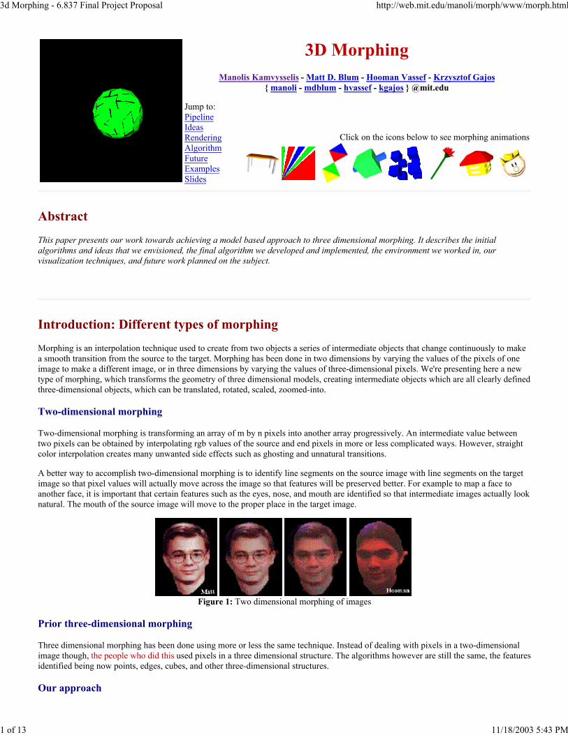
A better way to accomplish two-dimensional morphing is to identify line segments on the source image with line segments on the targetimage so that pixel values will actually move across the image so that features will be preserved better. For example to map a face toanother face, it is important that certain features such as the eyes, nose, and mouth are identified so that intermediate images actually looknatural. The mouth of the source image will move to the proper place in the target image.

Figure 1: Two dimensional morphing of images

Prior three-dimensional morphing

Three dimensional morphing has been done using more or less the same technique. Instead of dealing with pixels in a two-dimensionalimage though, the people who did this used pixels in a three dimensional structure. The algorithms however are still the same, the featuresidentified being now points, edges, cubes, and other three-dimensional structures.

Our approach


2 of 13 11/18/2003 5:43 PM

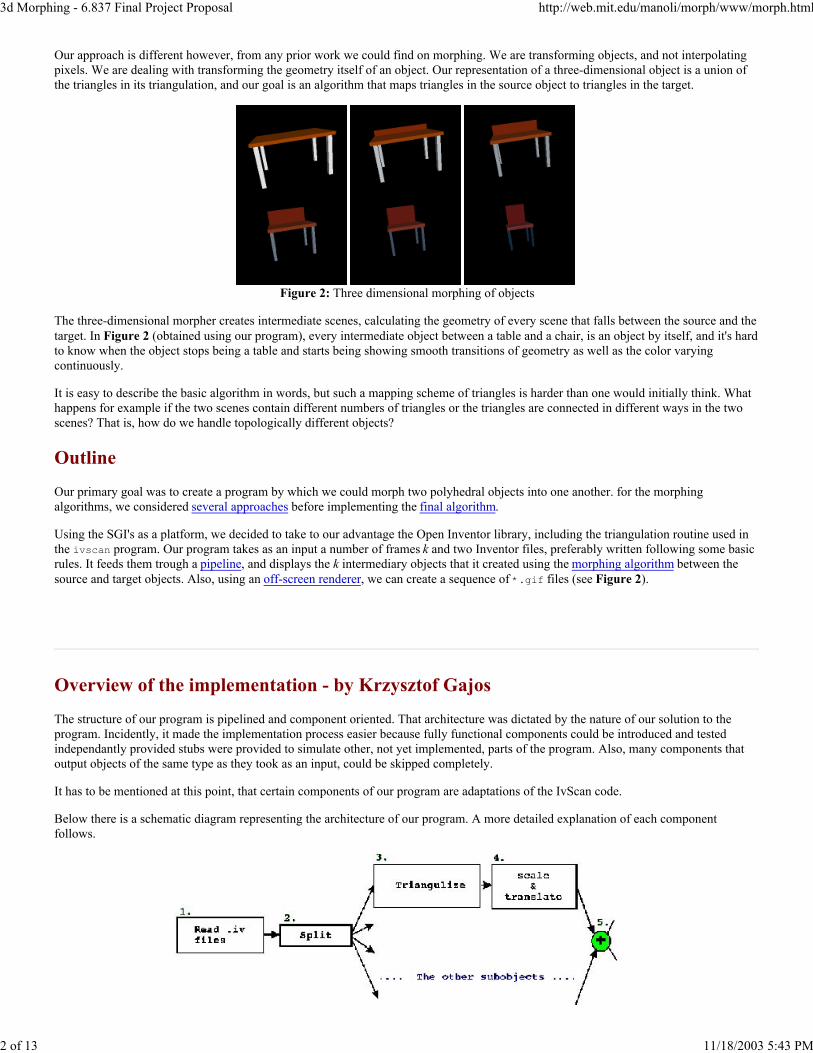
Our approach is different however, from any prior work we could find on morphing. We are transforming objects, and not interpolatingpixels. We are dealing with transforming the geometry itself of an object. Our representation of a three-dimensional object is a union ofthe triangles in its triangulation, and our goal is an algorithm that maps triangles in the source object to triangles in the target.

Figure 2: Three dimensional morphing of objects

The three-dimensional morpher creates intermediate scenes, calculating the geometry of every scene that falls between the source and thetarget. In Figure 2 (obtained using our program), every intermediate object between a table and a chair, is an object by itself, and it's hardto know when the object stops being a table and starts being showing smooth transitions of geometry as well as the color varyingcontinuously.

It is easy to describe the basic algorithm in words, but such a mapping scheme of triangles is harder than one would initially think. Whathappens for example if the two scenes contain different numbers of triangles or the triangles are connected in different ways in the twoscenes? That is, how do we handle topologically different objects?

Outline

Our primary goal was to create a program by which we could morph two polyhedral objects into one another. for the morphingalgorithms, we considered several approaches before implementing the final algorithm.

Using the SGI's as a platform, we decided to take to our advantage the Open Inventor library, including the triangulation routine used inthe ivscan program. Our program takes as an input a number of frames k and two Inventor files, preferably written following some basicrules. It feeds them trough a pipeline, and displays the k intermediary objects that it created using the morphing algorithm between the source and target objects. Also, using an off-screen renderer, we can create a sequence of *.gif files (see Figure 2).

Overview of the implementation - by Krzysztof Gajos

The structure of our program is pipelined and component oriented. That architecture was dictated by the nature of our solution to theprogram. Incidently, it made the implementation process easier because fully functional components could be introduced and testedindependantly provided stubs were provided to simulate other, not yet implemented, parts of the program. Also, many components thatoutput objects of the same type as they took as an input, could be skipped completely.

It has to be mentioned at this point, that certain components of our program are adaptations of the IvScan code.

Below there is a schematic diagram representing the architecture of our program. A more detailed explanation of each componentfollows.


3 of 13 11/18/2003 5:43 PM

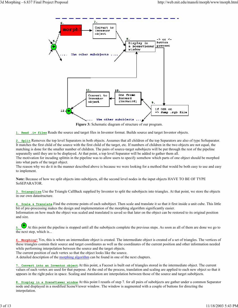
Figure 3: Schematic diagram of structure of our program.

1. Read .iv files Reads the source and target files in Inventor format. Builds source and target Inventor objects.

2. Split Removes the top level Separators in both objects. Assumes that all children of the top Separators are also of type SoSeparator.It matches the first child of the source with the first child of the target, etc. If numbers of children in the two objects are not equal, thematching is done for the smaller number of children. The pairs of source-target subobjects will be put through the rest of the pipelineseparatelly until they are to be displayed. At that point, a top level Separator will be added to gather them all. The motivation for incuding splittin in the pipeline was to allow users to specify somehow which parts of one object should be morphedinto what parts of the target object.The reason why we do it in the manner described above is because we were looking for a method that would be both easy to use and easyto implement.

Note: Because of how we split objects into subobjects, all the second level nodes in the input objects HAVE TO BE OF TYPESoSEPARATOR.

3. Triangulize Use the Triangle CallBack supplied by Inventor to split the subobjects into triangles. At that point, we store the objectsin our own datastructure.

4. Scale & Translate Find the extreme points of each subobject. Then scale and translate it so that it first inside a unit cube. This littlebit of pre-processing makes the design and implementation of the morphing algorithm significantly easier.Information on how much the object was scaled and translated is saved so that later on the object can be restored to its original positionand size.

5. At this point the pipeline is stopped until all the subobjects complete the previous steps. As soon as all of them are done we go tothe next step, which is...

6. Morphing! Yes, this is where an intermediate object is created. The intermediate object is created of a set of triangles. The vertices ofthese triangles contain their source and target coordinates as well as the coordinates of the current position and other information neededwhile performing interpolation between the source and the target objects. The current position of each vertex so that the object looks like the source.A detailed description of the morphing algorithm can be found in one of the next chapters.

7. Convert into an Inventor object At this point, a Faceset is built out of triangles stored in the intermediate object. The currentvalues of each vertex are used for that purpose. At the end of the process, translation and scaling are applied to each new object so that itappears in the right palce in space. Scaling and translation are interpolation between those of the source and target subobjects.

8. Display in a SceneViewer window At this point I resutls of step 7. for all pairs of subobjects are gather under a common Separatornode and displayed in a modified SceneViewer window. The window is augmented with a couple of buttons for directing theinterpolation.


4 of 13 11/18/2003 5:43 PM

9. If OSR is on => dump an .rgb file If the Off Screen Renderer flag is on, dump the current contents of the SceneViewer windowto an .rgb file so that it can be used for making movies. More information on the Off Screen Renderer and the movie making pipeline can be found in one of the next chapters.

10. One frame forward/backward Update the current position of each vertex in the intermediate structures corresponding to each of thesource-target subobject pairs. The new position corresponds to the next/previous frame in the morphing sequence. The values of thescaling and translating parameters are updated for each intermediate object as well.

11. Convert into an Inventor object Same as step 7.

12. Gathering all subobjects under a single Separator.

Possibilities for future improvements

Fuller handling of material properties. - At the moment the only material property that we do record and deal with is the diffuseColor. It would be desirable to include specular color, transparency, etc. for more pleasing effects.Finding Axis of Least Innertia - Let us imagine following input to our program: two sticks, one lying on the ground and the other standing up. At the moment, our program would morph the first stick into the second, by shrinking the first one in the X direction and expanding it in the Z direction. it is smooth and acceptable, though it would be much nicer if the stick rotated about the Y axis instead of growing and shrinking. In order to be able to achieve that, our program should be able to find an approximation to the axis of least inertia. We have actually designed a scheme that would handle the problem. The method would use the least squares approximation method to find the best fit line using only X and Y coordinates and another best fit line using only X and Z coordinates of the points. The first line would tell us the angle between the Z axis and the axis of least inertia and the other line would provide the angle between Y axis and the axis of least inertia.

That method is succeptible to errors and is only approximate but we believe it would be a good heuristic to work by. If the method were used, the objects would be rotated, before being scaled, translated and morphed, so that the computed axis of least inertia aligned with the Z axis. The rotation would be undone before dispalying the same way it is done wiht scaling and translation already.

A serious attempt had been made to solve that problem. Our team had acquired a copy of Matcomm software that provides an extensive library of math functions as well as a matlab to C++ compiler. We were not able to make the software fully functional (it would transalte but could not make libraries accessible for compilation) without installing it permanently on an SGI workstation. We may work on alternative methods.

Morphing Algorithms - by Manolis Kamvysselis and Hooman Vassef

In all the approaches we considered, the morphing process required some sort of matching between the triangles in the source an targetobjects, then transformations within these matches.

Explored approaches for the transformations

Consider the case where one polygon (triangle) maps to many. We must somehow create new triangles, and we considered twoapproaches: "shaping" and "spawning". The first one tries to shape a set of triangles inside the source triangle, the second one spawns allthe extra triangles off the edges of the source triangle.

But first, here is a description of how we spawn a vertex from an edge, a process that both approaches use.

Spawning a vertex comes down to creating a zero-area triangle with two vertices shared with an existantedge of the nearest source triangle, and a third vertex at its middle (or some nicer ratio).

Nicer ratio: suppose we need to place point A on an edge BC knowing that the whole will evolve into atriangle A'B'C'. We take the ratio A'B'/A'C', and we set A on BC such that it's the same as AB/AC.

Figure 4: Spawning a vertex


5 of 13 11/18/2003 5:43 PM

Shaping (Hooman)

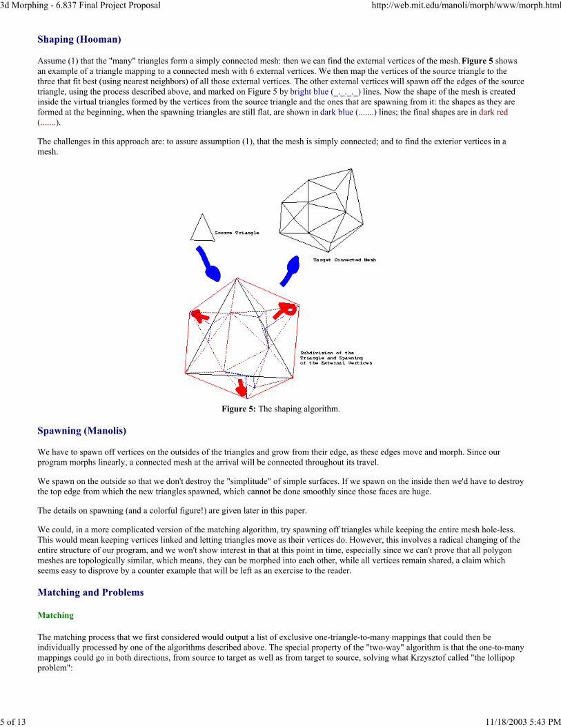
Assume (1) that the "many" triangles form a simply connected mesh: then we can find the external vertices of the mesh. Figure 5 showsan example of a triangle mapping to a connected mesh with 6 external vertices. We then map the vertices of the source triangle to thethree that fit best (using nearest neighbors) of all those external vertices. The other external vertices will spawn off the edges of the sourcetriangle, using the process described above, and marked on Figure 5 by bright blue (_._._._) lines. Now the shape of the mesh is createdinside the virtual triangles formed by the vertices from the source triangle and the ones that are spawning from it: the shapes as they areformed at the beginning, when the spawning triangles are still flat, are shown in dark blue (.......) lines; the final shapes are in dark red (.......).

The challenges in this approach are: to assure assumption (1), that the mesh is simply connected; and to find the exterior vertices in amesh.

Figure 5: The shaping algorithm.

Spawning (Manolis)

We have to spawn off vertices on the outsides of the triangles and grow from their edge, as these edges move and morph. Since ourprogram morphs linearly, a connected mesh at the arrival will be connected throughout its travel.

We spawn on the outside so that we don't destroy the "simplitude" of simple surfaces. If we spawn on the inside then we'd have to destroythe top edge from which the new triangles spawned, which cannot be done smoothly since those faces are huge.

The details on spawning (and a colorful figure!) are given later in this paper.

We could, in a more complicated version of the matching algorithm, try spawning off triangles while keeping the entire mesh hole-less.This would mean keeping vertices linked and letting triangles move as their vertices do. However, this involves a radical changing of theentire structure of our program, and we won't show interest in that at this point in time, especially since we can't prove that all polygonmeshes are topologically similar, which means, they can be morphed into each other, while all vertices remain shared, a claim whichseems easy to disprove by a counter example that will be left as an exercise to the reader.

Matching and Problems

Matching

The matching process that we first considered would output a list of exclusive one-triangle-to-many mappings that could then beindividually processed by one of the algorithms described above. The special property of the "two-way" algorithm is that the one-to-manymappings could go in both directions, from source to target as well as from target to source, solving what Krzysztof called "the lollipopproblem":


6 of 13 11/18/2003 5:43 PM

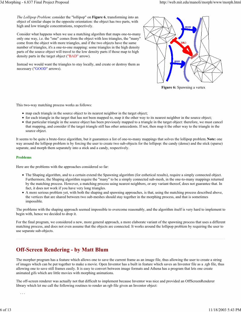
The Lollipop Problem: consider the "lollipop" on Figure 6, transforming into an object of similar shape in the opposite orientation: the object has two parts, withhigh and low triangle concentrations, respectively.

Consider what happens when we use a matching algorihm that maps one-to-manyonly one way, i.e. the "one" comes from the object with less triangles, the "many"come from the object with more triangles, and if the two objects have the samenumber of triangles, it's a one-to-one mapping: some triangles in the high densityparts of the source object will travel to the low density parts if those map to highdensity parts in the target object ("BAD" arrow).

Instead we would want the triangles to stay locally, and create or destroy them asnecessary ("GOOD" arrows).

Figure 6: Spawning a vertex

This two-way matching process works as follows:

map each triangle in the source object to its nearest neighbor in the target object;for each triangle in the target that has not been mapped to, map it the other way to its nearest neighbor in the source object;that particular triangle in the source object has been previously mapped to a triangle in the target object: therefore, we must cancelthat mapping, and consider if the target triangle still has other antecedents. If not, then map it the other way to the triangle in thesource object.

It seems to be quite a brute-force algorithm, but it guarantees a list of one-to-many mappings that solves the lollipop problem. Note: one way around the lollipop problem is by forcing the user to create two sub-objects for the lollipop: the candy (dense) and the stick (sparse)separate, and morph them separately into a stick and a candy, respectively.

Problems

Here are the problems with the approaches considered so far:

The Shaping algorithm, and to a certain extend the Spawning algorithm (for esthetical results), require a simply connected object.Furthermore, the Shaping algorithm require the "many" to be a simply connected sub-mesh, in the one-to-many mappings returnedby the matching process. However, a matching process using nearest neighbors, or any variant thereof, does not guarantee that. Infact, it does not work if you have very long triangles.A more serious problem yet, with both the shaping and spawning approaches, is that, using the matching process described above,the vertices that are shared between two sub-meshes should stay together in the morphing process, and that is sometimesimpossible.

The problems with the shaping approach seemed impossible to overcome reasonably, and the algorithm itself is very hard to implement tobegin with, hence we decided to drop it.

For the final program, we considered a new, more general approach, a more elaborate variant of the spawning process that uses a differentmatching process, and does not even assume that the objects are connected. It works around the lollipop problem by requiring the user touse separate sub-objects.

Off-Screen Rendering - by Matt Blum

The morpher program has a feature which allows one to save the current frame as an image file, thus allowing the user to create a stringof images which can be put together to make a movie. Open Inventor has a built in feature which saves an Inventor file as a .rgb file, thusallowing one to save still frames easily. It is easy to convert between image formats and Athena has a program that lets one createanimated gifs which are little movies with morphing animations.

The off-screen renderer was actually not that difficult to implement because Inventor was nice and provided an OffScreenRendererlibrary which let me call the following routines to render an rgb file given an Inventor object:

...


7 of 13 11/18/2003 5:43 PM

SoOffscreenRenderer *myRenderer = new SoOffscreenRenderer(myViewport); myRenderer->setBackgroundColor(SbColor(0,0,0)); /* black background */ if (!myRenderer->render(root)) { delete myRenderer; return FALSE; } /* output .rgb file */ FILE *fp = fopen(outputfile, "w"); myRenderer->writeToRGB (fp); ...

One little problem I experienced initially with the off-screen renderer was the requirement that the whole scene be under a singleSeparator node, but since our objects behaved this rule to begin with, it was not a problem. Another small problem with the OSR was thatit also initially needed a camera and light position specified in separate files camera.iv and light.iv, but the Inventor libraries in C++provide routines to dynamically get the camera and lighting information to produce a decent scene. Without this information, the OSRcamera position may default to a position pointing away from the object, which would not be very useful.

After getting the OSR to work properly all the time, I incorporated the code as a procedure in the main morphing program and added abutton on the main interface that will render the current scene immediately as an rgb file sceneX.rgb where X is the current framenumber. The morpher keeps track of the current frame from 1 to N so the frames will be always saved in the correct order.

Thus when the morphing was done, there would be a bunch of files frame1.rgb, frame2.rgb, ..., frameN.rgb which needed to be strungtogether in a movie. There is a utility on Athena called whirlgif which takes a group of .gif files and makes an animated gif from them(which is easily viewable in Netscape or any other web browser).

The last issue that remained was to convert from .rgb to .gif and there was no converter available. However, doing "man rgb" showed ashort 20 line C program on how to read a .rgb file and get its contents. Writing gifs is hard (because it involves a solid knowledge ofLZW encoding and a lot of bit manipulation), but writing a .ppm is easy (it is just a string of red, green, blue values) and there is a utilityon Athena to convert ppms to gifs, so combining all these tools, I wrote a little script called rgbtogif.

Now that I could make gifs from rgbs, I wrote a short script called makemovie which automatically senses all the files of the formframeX.rgb, converts them into gifs and strings them into an animated gif movie.

Interface between Open Inventor and Morphing

We want our morphing algorithm to have a natural user-friendly interface and also be interactive, requiring it to do graphics rendering onthe fly. Originally, we thought about having a program to take in two sets of triangles each of a specific format because all of ourmorphing algorithms mapped triangles to triangles. However, if we wanted to have the morpher handle more complicated objects such ascubes, cylinders or spheres, we would have to first manually convert these to triangles to run them through the morpher.

Ideally, we wanted a program that would take objects of a high-level language (such as Inventor format), and morph them interactively.We then realized that in Assignment 4, we used a scan converter that took an OpenInventor file and automatically triangulized it. Usingthis, it was then easy to put these triangles into our data structures for the morphing algorithm. Since SceneViewer is easily extendible, wecould write an extension of SceneViewer by adding a couple extra buttons to handle morphing interactively.

The interface we then decided on was to have the program read in a source and target Inventor files on the command line, bring up aSceneViewer window with added buttons "->" and "<-" to flip forward or backward through the stages of morphing. We set a morphingparameter k that went from 0 to N where k=0 is the source and k=N is the target and the other values represent intermediate scenes. Onceall the geometry was calculated at the beginning and the nearest neighbor, all the mappings were completed, then creating intermediatescenes varying k was very fast. In fact, we could have SceneViewer render the intermediate scene on the fly, so as one repeatedly clickedthe "->" button, he could see the object morphing continuously.

Later we added another option on the command line, which was the number of frames N or discrete steps k made. Large values made forsmoother morphing with more frames. Finally we added a little button to do the off-screen rendering. When one clicks this button, theOSR would render the current scene, keeping track of the index k and rendering an image called "image(k).rgb".

We also included a -debug option on the command line which would print out a verbose report on all the steps the morpher went throughso that if it had a problem, the problem could be pinpointed much easier. It is annoying to run a large program and all you see is"segmentation fault" and you have no idea where it broke. The -debug option also shows all the nearest neighbor calculations and how itmatched vertices from the source to the target.

The Algorithm - by Manolis Kamvysselis


8 of 13 11/18/2003 5:43 PM

We're describing in this part the low-level algorithm to match m polygons to n polygons, without preserving any structure. Note that thestructure in our structured morpher is obtained by calling this unstructured morphing algorithm iteratively on parts of the scene that theuser has specified he/she wants to map to each other, as described earlier in this paper.

We'll also note that we're mapping objects which have been scaled and translated, such that their xyz bounding box is a unit cube centeredat the origin.

Motivation

Two techniques (shaping and spawning) were already presented for creating new polygons. The same techniques apply for makingpolygons disappear (since one can reverse source and destination environments when doing the matching to guarantee creation instead ofdeletion of polygons).

Consider however a morphing alorithm which has no cost assigned to those creations and deletions. In an extreme such case, the programwould minimize to zero the old shapes, and create from zero the new shapes. We've taken all intelligence and progressivity out ofmorphing. We'll try and stay as far away from this as possible.

Thus, our main concern will be minimizing creation and deletion of polygons. Therefore we'll map as many polygons as we can in aone-to-one mapping, and only afterwards will we spawn off the rest as needed.

We'll start by examining the M-to-M mapping first, where m is the min number of polygons among the source and the target. We'll thenintroduce the Edge Ordering algorithm for doing such a mapping. Afterwards we'll examine the M to N mapping, and describe how newtriangles spawn off in the scene. Finally we'll describe the Incremental Edge Ordering algorithm, an extension to our original EdgeOrdering algorithm.

M to M mapping

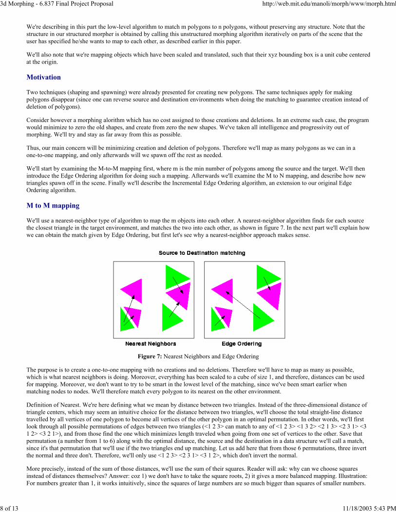
We'll use a nearest-neighbor type of algorithm to map the m objects into each other. A nearest-neighbor algorithm finds for each sourcethe closest triangle in the target environment, and matches the two into each other, as shown in figure 7. In the next part we'll explain howwe can obtain the match given by Edge Ordering, but first let's see why a nearest-neighbor approach makes sense.

Figure 7: Nearest Neighbors and Edge Ordering

The purpose is to create a one-to-one mapping with no creations and no deletions. Therefore we'll have to map as many as possible,which is what nearest neighbors is doing. Moreover, everything has been scaled to a cube of size 1, and therefore, distances can be usedfor mapping. Moreover, we don't want to try to be smart in the lowest level of the matching, since we've been smart earlier whenmatching nodes to nodes. We'll therefore match every polygon to its nearest on the other environment.

Definition of Nearest. We're here defining what we mean by distance between two triangles. Instead of the three-dimensional distance oftriangle centers, which may seem an intuitive choice for the distance between two triangles, we'll choose the total straight-line distancetravelled by all vertices of one polygon to become all vertices of the other polygon in an optimal permutation. In other words, we'll firstlook through all possible permutations of edges between two triangles (<1 2 3> can match to any of <1 2 3> <1 3 2> <2 1 3> <2 3 1> <31 2> <3 2 1>), and from those find the one which minimizes length traveled when going from one set of vertices to the other. Save thatpermutation (a number from 1 to 6) along with the optimal distance, the source and the destination in a data structure we'll call a match,since it's that permutation that we'll use if the two triangles end up matching. Let us add here that from those 6 permutations, three invertthe normal and three don't. Therefore, we'll only use <1 2 3> <2 3 1> <3 1 2>, which don't invert the normal.

More precisely, instead of the sum of those distances, we'll use the sum of their squares. Reader will ask: why can we choose squaresinstead of distances themselves? Answer: coz 1) we don't have to take the square roots, 2) it gives a more balanced mapping. Illustration:For numbers greater than 1, it works intuitively, since the squares of large numbers are so much bigger than squares of smaller numbers.


9 of 13 11/18/2003 5:43 PM

Example: sum of 1 10 1 is 12 in sum of distances, and 102 in sum of distances squared. However, 4 4 4 has a sum of distances of also 12,but a sum of squares of 48, which is largely smaller than 102. Therefore, for numbers greater than 1, a more balanced mapping would bechosen. Even though some may find it counter-intuitive, this reasoning also works for numbers which are all smaller than 1 (which is thecase in our program, since we're scaling everything to a cube of size 1 when doing the mapping). Example, in the case of .01 .01 and .1,the sum of squares is .0102 while the sum of the numbers is .12. For the same sum .12 we could have .04 .04 and .04, in which case thesum of squares would become .0048, which is smaller than .0102, therefore the balanced thing will stll get chosen. A simple argument(convince yourselves, just like we did) is that we can scale everything by 1000 maintaining ratios, and since the scaling is uniform andcan be eliminated in the inequality, we're still comparing squares of #'s bigger than 1. We'll therefore use sum of squares that yield morebalanced travels.

However, a nearest-neighbor algorithm doesn't guarantee we'll have unique matches for each polygon, as one can see in figure 7. We'llcall conflict a match which shares its source or its target with another match. An extended nearest neighbor would work if it has someway of resolving conflicts. It must either either resolve conflicts at the end, which can take a very long time and algorithms for which riskto be very complicated and recurse indefinitely, or if it can resolve conflicts incrementally, by mapping to the nearest polygon which isnot already matched with another, in which case the algorithm is partial since it will match the nodes visited first without guaranteeing aglobally optimal matching.

Edge Ordering

An alternative to a nearest-neighbor algorithm is the Edge Ordering Algorithm, introduced in 1997 by Manolis Kamvysselis, a junior incomputer science at MIT. He originally used it for his final project in Computer Graphics, and we'll use it here, since it seems fit.

In this algorithm, each triangle is a node, and each matching between two triangles is an edge between two nodes. Since matchings aredone only between the two non-intersecting spanning sets of sources and targets, the matching problem becomes the construction of abipartite graph which connects all nodes, and each node only once.

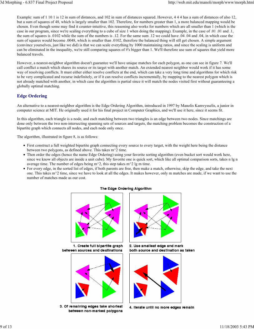
The algorithm, illustrated in figure 8, is as follows:

First construct a full weighted bipartite graph connecting every source to every target, with the weight here being the distancebetween two polygons, as defined above. This takes m^2 time.Then order the edges (hence the name Edge Ordering) using your favorite sorting algorithm (even bucket sort would work here,since we know all objects are inside a unit cube). My favorite one is quick sort, which like all optimal comparison sorts, takes n lg naverage time. The number of edges being m^2, this step takes m^2 lg m time.For every edge, in the sorted list of edges, if both parents are free, then make a match, otherwise, skip the edge, and take the nextone. This takes m^2 time, since we have to look at all the edges. It makes however, only m matches are made, if we want to use thenumber of matches made as our cost.


10 of 13 11/18/2003 5:43 PM

Figure 7: The Edge Ordering Algorithm

Correctness: When no more edges remain in our sorted list, we'll have achieved our bipartite graph. Proof: suppose at least one pair isunmatched. since our list contained an edge for every pair of nodes, it must have either not seen their edge (therefore we're not done,contradiction), or seen their edge and didn't connect them (therefore, one of the nodes must have been taken, therefore no unmatched pairof nodes exist).

Greedy strategy is optimal in polynomail time. The problem of finding the minimum length cycle in the full bipartite graph is NP hard,therefore, we can't wish to achieve an optimally optimal solution. However, our greedy approach does pretty well for its running time,since at each step it's adding the minimum weight edge available.

M to N mapping

We assume we've already mapped m polygons to m others, and there remain n-m of them unmatched all in the same environment (bycorrectness argument) either in the source or in the target environment, without loss of generality.

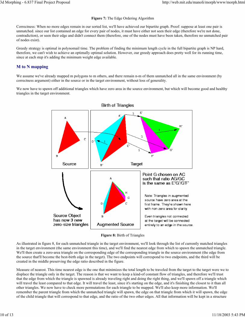
We now have to spawn off additional triangles which have zero area in the source environment, but which will become good and healthytriangles in the target environment.

Figure 8: Birth of Triangles

As illustrated in figure 8, for each unmatched triangle in the target environment, we'll look through the list of currently matched trianglesin the target environment (the same environment this time), and we'll find the nearest edge from which to spawn the unmatched triangle.We'll then create a zero-area triangle on the corresponding edge of the corresponding triangle in the source environment (the edge fromthe source that'll become the best-birth edge in the target). The two endpoints will correspond to two endpoints, and the third will becreated in the middle preserving the edge ratio described in the figure.

Measure of nearest. This time nearest edge is the one that minimizes the total length to be traveled from the target to the target were we todisplace the triangle only in the target. The reason is that we want to keep a kind-of constant flow of triangles, and therefore we'll trustthat the edge from which the triangle is spawned is already traveling right and doing the right thing, and we'll spawn off a triangle whichwill travel the least compared to that edge. It will travel the least, since it's starting on the edge, and it's finishing the closest to it than allother triangles. We now have to check more permutations for each triangle to be mapped. We'll also keep more information. We'llremember the parent triangle from which the unmatched triangle will spawn, the edge on that triangle from which it will spawn, the edgeof the child triangle that will correspond to that edge, and the ratio of the two other edges. All that information will be kept in a structure


11 of 13 11/18/2003 5:43 PM

we'll call a birth.

Incremental Edge Ordering Algorithm

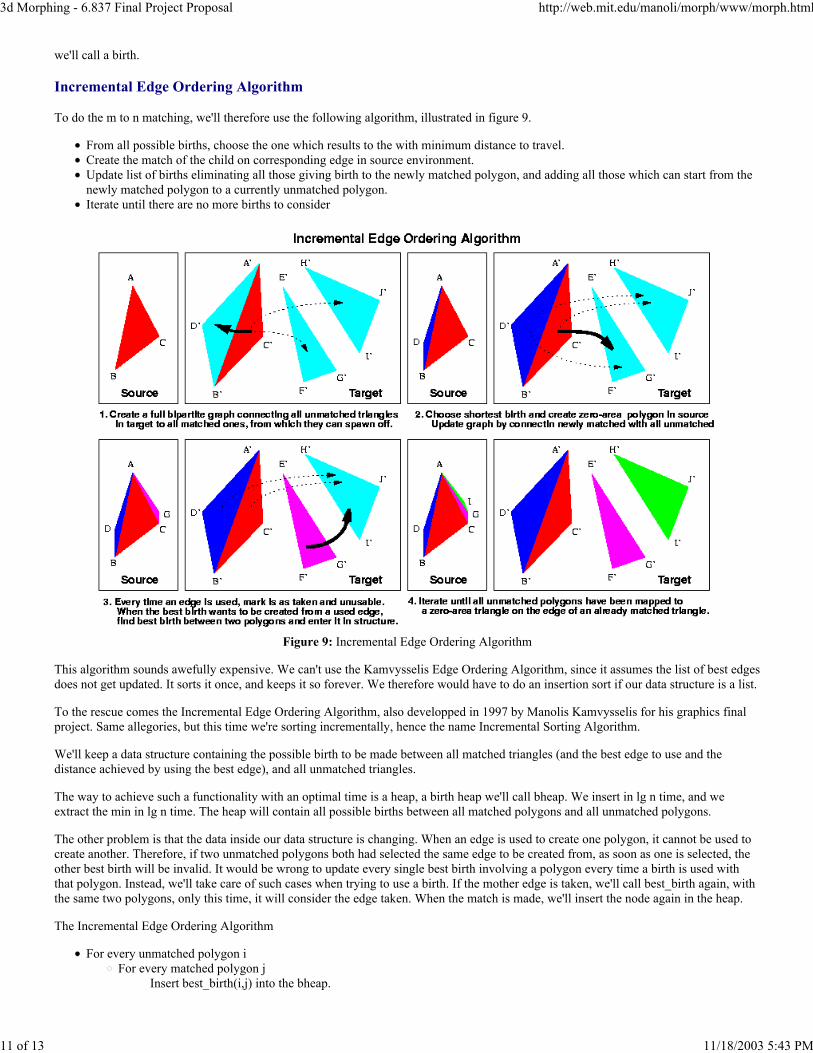
To do the m to n matching, we'll therefore use the following algorithm, illustrated in figure 9.

From all possible births, choose the one which results to the with minimum distance to travel.Create the match of the child on corresponding edge in source environment.Update list of births eliminating all those giving birth to the newly matched polygon, and adding all those which can start from thenewly matched polygon to a currently unmatched polygon.Iterate until there are no more births to consider

Figure 9: Incremental Edge Ordering Algorithm

This algorithm sounds awefully expensive. We can't use the Kamvysselis Edge Ordering Algorithm, since it assumes the list of best edgesdoes not get updated. It sorts it once, and keeps it so forever. We therefore would have to do an insertion sort if our data structure is a list.

To the rescue comes the Incremental Edge Ordering Algorithm, also developped in 1997 by Manolis Kamvysselis for his graphics finalproject. Same allegories, but this time we're sorting incrementally, hence the name Incremental Sorting Algorithm.

We'll keep a data structure containing the possible birth to be made between all matched triangles (and the best edge to use and thedistance achieved by using the best edge), and all unmatched triangles.

The way to achieve such a functionality with an optimal time is a heap, a birth heap we'll call bheap. We insert in lg n time, and weextract the min in lg n time. The heap will contain all possible births between all matched polygons and all unmatched polygons.

The other problem is that the data inside our data structure is changing. When an edge is used to create one polygon, it cannot be used tocreate another. Therefore, if two unmatched polygons both had selected the same edge to be created from, as soon as one is selected, theother best birth will be invalid. It would be wrong to update every single best birth involving a polygon every time a birth is used withthat polygon. Instead, we'll take care of such cases when trying to use a birth. If the mother edge is taken, we'll call best_birth again, withthe same two polygons, only this time, it will consider the edge taken. When the match is made, we'll insert the node again in the heap.

The Incremental Edge Ordering Algorithm

For every unmatched polygon iFor every matched polygon j

Insert best_birth(i,j) into the bheap.


12 of 13 11/18/2003 5:43 PM

Until no more polygons are unmatched ( O(n-m))Choose the birth with the smallest dist. ( O(lg ((n+m)*(n-m))) )1.If the child polygon is already matched, skip. loop.2.If the parent edge is taken, call best_birth on parent and child and insert birth into data structure, loop.3.Otherwise make birth happen. Mark the unmatched polygon as matched, and find best_births for each of the remainingunmatched polygons and insert them into the births heap. ( O (m * lg ((n+m)*(n-m))) )

4.

Mark the edge that gave birth as taken. Mark the edge that was born as also taken. The other two edges of new polygon cangive birth to unmatched polygons also.

5.

Correctness: at any time, at least all possible births are included in the data structure, and the optimal one is handed in by the call tobheap_return_min. No impossible birth will be made between two polygons, since we're checking all criteria that would disallow thematch. If, when the edge of a parent is already used, we're reconstructing a birth among those two polygons, we're guaranteed that it won'tbe better than any birth already used, since it's not better than the previous birth between those two polygons (otherwise, it would havebeen selected in the first time around), and the impossible birth is no better than any of the ones already used otherwise, it would havebeen extracted from the bheap earlier. Putting the new reconstructed birth and back, guarantees that if the birth leads to an optimalcombination later on, it will get selected.

Greediness: by arguments above, at each step we're making the optimal choice for a birth. Finding the one best combination is howeverNP hard, and we're doing pretty well for a polygomial (times logarithmic) time.

Possibilities for future improvements

An interesting extension to our three-dimensional morpher could be a hybrid between two and three-dimensional morphing by alsoincluding morphing of texture maps between objects. In most applications, scenes are rendered as simple objects but with complicatedtextures and morphing of texture maps would help to make the transition appear even more realistic.

Lessons Learned or How We Benefited From Doing This Project

Open Inventor - Through working on this project we had a chance to become intimately familiar with the Open Inventor. The first discovery that we made about it was that Open Inventor was not a closed program or system but an extensive collection of tools accessible to programmers.Morphing - We researched the field and learned about many interesting things that other people are doing. Unfortunatelly, we did not find any papers that were directly applicable to our problem. On the other hand, that allowed us to build an entirely new and entirely our own solution! Very rewarding. Let's get some patents on those nice algorithms! Free ticket to SIGGRAPH '99 after graduation :o)Software Engineering - For most of us it was a second team project in software developement. We learned a lot about how a team should work and what are the efficient and ineffictient ways of managind code and work.

Individual contributions (division of labor)

Matt - Off Screan Renderer, parsing command line arguments, movie-making pipeline, the 2D morphing demo for our front page.Manolis - Morphing - Matching - Edge Ordering Algorithm - Incremental Edge Ordering AlgorithmHooman - MorphingKrzysztof - Everything else, i.e. all of the pipeline described above except for the morphing and OSR.

Acknowledgements

The team would like to thank Jonathan Levene, the god of Inventor, who was a non-exhaustable source of insipration in our struggles with Open Inventor.

The team would also like to express its gratitude towards our project supervisor, Luke Weisman, for his patience (when needed), impatience (when nothing else worked), and cool ideas.

We would also like to thank our friends, brothers, sisters, parents, roomates, pets, stuffed animals, and last but not least the TA's of other classes too, who supported our efforts of spending endless hours on this project. Thanks!

Finally, the team would like to thank the Anonymous Genius who wrote the IvScan. A lot of our knowledge about the Open Inventor as well as numerous parts of our code come from his work.

Bibliography


13 of 13 11/18/2003 5:43 PM

The Inventor Mentor: Programming Object-Oriented 3D Graphics with Open Inventor, Release 2; SGI On-Line edition

The Team: MaD-HooK [email protected]

Manolis Kamvysselis Matt D. Blum Hooman Vassef Krzysztof Gajosmanoli mdblum hvassef kgajos

Final Project for 6.837, Computer Graphics. Professor: Seth Teller ([email protected]) TA: Luke Weisman([email protected])

Documents

3d Morphing - 6.837 Final Project Proposalcompbio.mit.edu/publications/I03_Kamvysselis_3Dmorph_97.pdf · 3d Morphing - 6.837 Final Project Proposal 3 of 13 11/18/2003 5:43 PM Figure