Copyright © 2019 by Author/s and Licensed by Modestum Ltd., UK. This is an open access article distributed under the Creative Commons Attribution License which permits unrestricted use, distribution, and reproduction in any medium, provided the original work is properly cited.

European Journal of Sustainable Development Research 2019, 3(2), em0081 ISSN: 2542-4742

3D Model Reconstruction from Two Orthographic Views using Fuzzy Surface Analysis

Hamid Haghshenas Gorgani 1, Alireza Jahantigh Pak 2, Sadegh Sadeghi 3*

1 Engineering Graphics Center, Sharif University of Technology, Tehran, IRAN 2 Head of Engineering Graphics Center, Sharif University of Technology, Tehran, IRAN 3 Department of Mechanical Engineering, Iran University of Science and Technology, Tehran, IRAN *Corresponding Author: sadeghsadeghi@mecheng.iust.ac.ir Citation: Gorgani, H. H., Pak, A. J. and Sadeghi, S. (2019). 3D Model Reconstruction from Two Orthographic Views using Fuzzy Surface Analysis. European Journal of Sustainable Development Research, 3(2), em0081. https://doi.org/10.29333/ejosdr/5726 Published: March 3, 2019 ABSTRACT The need for revision, the difficulty of visualization, and the impossibility of using 2D drawings as the input of manufacturing machines make us attempt to acquire a 3D model from 2D engineering drawings. However, the main problem in this process is that we encounter many potential uncertainties. In this paper, to overcome this problem, we used the fuzzy logic as a mathematical tool based on knowledge of an expert. One of the most outstanding advantages of using the fuzzy logic is that uncertainty in related equivalent elements in different orthographic views is reduced. Another important feature of this method is that only two orthographic views are used to reconstruct the 3D model, while in previous methods, three orthographic views were used. Reducing the limitations of reconstruction of 3D models will result lower cost because of simulation of production processes on a 3D model and direct connection to CAD/CAM Systems, conservation of natural resources and more security for documents by maintaining drawings in computer memory, improved education quality and increased health level as a result of better visualization using 3D Object which will ultimately lead to sustainable development.

Keywords: 3D reconstruction, fuzzy logic, surface analysis, engineering drawing, sustainable development

INTRODUCTION

Since the 18th century, when the projection theory and the descriptive geometry were introduced and used to solve engineering problems, 2D drawings were established in engineering design processes (Jeon et al., 2016; Lee and Han, 2005). Multi-view 2D drawings are not just a powerful presentation of the 3D object but a standard environment between design and manufacturing (Wen et al., 2015) as well and are sometimes used as the principal element showing the production and assembling process (Lee and Han, 2005; Wen et al., 2017a, 2017b). In today's societies, due to the limited resources of energy and so the need to quick production processes, the use of automatic systems is necessary (Banapurmath et al., 2018). It also leads to sustainable development that is essential for the modern economy (Elnashaie et al., 2018). In general, an accurate estimation of the geometric condition of the system can lead to a better understanding of the system's behavior and to prevent its possible and potentially harmful effects (Haghshenas et al., 2018; Jianu and Rosen, 2017; Shahriari et al., 2018). Most contemporary products are described using 2D drawings (Wang and Grinstein, 1993), however, since revising older product designs is a necessity, there are some unavoidable limitations to this type of drawing, some of which are as follows:

Gorgani et al. / 3D Model Reconstruction from Two Orthographic Views

2 / 13 © 2019 by Author/s

• Visualization in the form of 3D objects and the direct use of a 2D drawing without having its physical model is extremely difficult (Gorgani, 2016a);

• 2D drawings cannot be used as input for today’s manufacturing systems, and applications such as the analysis and prototyping are extremely difficult for them (Wang and Latif, 2007);

• Revision of 2D drawings is extremely time and cost consuming (Bai et al., 2010). Given the above limitations, obtaining 3D models from 2D drawings becomes very important (Biasotti et al.,

2016; Lahner et al., 2016). Obtaining 2D orthographic views form 3D models is a movement from high-level information to low-level information, and it is an easy procedure; however, since reconstructing 3D models from orthographic views is a movement from low-level information to high-level information, it is an extremely difficult task (Mura et al., 2016; Mura et al., 2014; Ochmann et al., 2016; Stephan and Cordy, 2013) . Such problems become more apparent when we start to realize that a lot of information is lost in the process of obtaining orthographic views from 3D models. Methods presented to reconstruct 3D models from 2D orthographic views can be categorized as follows:

• The B-Rep method (Boundary representation) (Bezdek, 1994; Shin and Shin, 1998; Soni and Gurumoorthy, 2003);

• The CSG method (Constructive Solid Geometry) (Aldefeld, 1983). The B-Rep method was started by Ideas and continued to develop by others (Sakurai and Gossard, 1983). This

method, which is a bottom-up method, can be described by the following steps (Sakurai and Gossard, 1983): 1. Transforming 2D vertices into 3D vertices; 2. Creating 3D line segments from 3D vertices; 3. Creating faces from 3D line segments; 4. Making 3D objects from faces.

The CSG method, a top-down method started by Aldefeld (1983), can also be explained as follows: 1. Obtaining 3D primary volumes from 2D drawings; 2. Performing Boolean operations on 3D primitives and identifying their participation; 3. Creating 3D solid as the final object.

While both of the above methods have good efficiency, they have serious problems as well. Compared with

CSG, the B-Rep method encompasses a wider range of shapes but cannot analyze complicated ones and encounters some uncertainties (Geng et al., 2002). Since it uses Boolean operations, CSG is more efficient in presenting unique solutions (López-Sastre et al., 2013). However, since it uses basic primary shapes to reconstruct 3D objects, it has serious limitations when dealing with complicated shapes.

In both methods, the most serious problem occurs when we want to correlate elements in two different orthographic views (Jiang and Fu, 2011; Su et al., 2013). In fact, this problem appears when there is uncertainty and we need expert opinion and knowledge (Haghshenas et al., 2018; Wang et al., 2013). One of the most important applications of the fuzzy logic theory as a mathematical method is to correlate vague data sets by making use of expert knowledge (Ross, 2009). This theory was first introduced in 1965 by Professor L. A. Zadeh (1965) and has since become a link between humans and computers, which helps to minimize conflicts in this relation (Dubois and Prade, 1993). Based on this theory, factors and ranges can be categorized without having any precise boundary. The fuzzy logic theory is very useful for solving real-world problems. Vague variables and their impact on the system are called ‘psycho-linguistic variables’. This theory can thus be used in various fields such as calculus, topology, the humanities, experimental sciences, engineering, and, in general, wherever expert knowledge is needed (Dubois and Prade, 1993; Gorgani et al., 2017).

In this paper, first, two orthographic views are collated. Using the surface analysis method, two different orthographic views of the two-dimensional object are interconnected. This method is, in fact, a mathematical method based on expert knowledge and is thus precise and flexible. Furthermore, in case 2D engineering drawings are scratched, this method can offer an approximate model for the 3D object. Another advantage is that only two orthographic views are used to reconstruct the 3D model while in methods presented so far, 3 orthographic views have been used. So, we can claim that “the degree of ideality” of our system has improved (Gorgani, 2016b).

One of the limitations of this method, however, is that it can be applied only to models with planar faces and does not include curved faces.

European Journal of Sustainable Development Research, 3(2), em0081

© 2019 by Author/s 3 / 13

EXPERT KNOWLEDGE: INTRODUCTION TO SURFACE ANALYSIS

The first and most difficult stage in the reconstruction of a three-dimensional object from two-dimensional orthographic views is to find the equivalent components in different views. To do this, we use the surface analysis method (Mottaghipour et al., 2018; Mottaghipour et al., 2017), described with an example as follows:

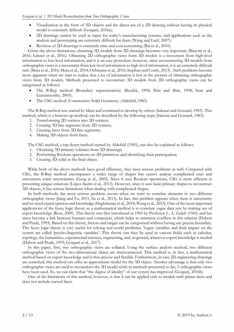
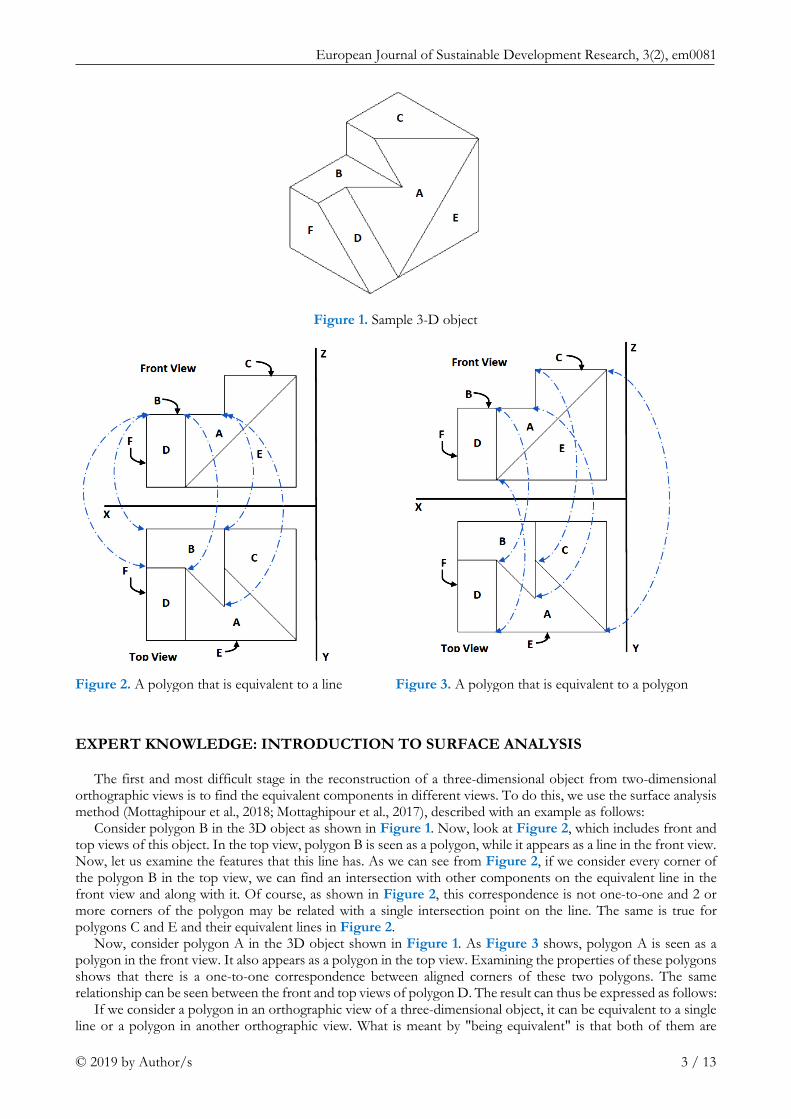
Consider polygon B in the 3D object as shown in Figure 1. Now, look at Figure 2, which includes front and top views of this object. In the top view, polygon B is seen as a polygon, while it appears as a line in the front view. Now, let us examine the features that this line has. As we can see from Figure 2, if we consider every corner of the polygon B in the top view, we can find an intersection with other components on the equivalent line in the front view and along with it. Of course, as shown in Figure 2, this correspondence is not one-to-one and 2 or more corners of the polygon may be related with a single intersection point on the line. The same is true for polygons C and E and their equivalent lines in Figure 2.

Now, consider polygon A in the 3D object shown in Figure 1. As Figure 3 shows, polygon A is seen as a polygon in the front view. It also appears as a polygon in the top view. Examining the properties of these polygons shows that there is a one-to-one correspondence between aligned corners of these two polygons. The same relationship can be seen between the front and top views of polygon D. The result can thus be expressed as follows:

If we consider a polygon in an orthographic view of a three-dimensional object, it can be equivalent to a single line or a polygon in another orthographic view. What is meant by "being equivalent" is that both of them are

Figure 1. Sample 3-D object

Figure 2. A polygon that is equivalent to a line Figure 3. A polygon that is equivalent to a polygon

Gorgani et al. / 3D Model Reconstruction from Two Orthographic Views

4 / 13 © 2019 by Author/s

different orthographic views of a single polygon. If the equivalent image is a polygon, it is necessary to have a one-to-one correspondence between the corners of this polygon and the first polygon corners. If, on the other hand, the equivalent image is a line, there must be an intersection point on the line in the direction of each of the first polygon corners. (This correspondence is not necessarily one-to-one, of course). Now, using this principle, we will create the necessary formulas and fuzzy rules in the proposed method.

DEFINITION OF VARIABLES AND ALGEBRAIC PHRASES

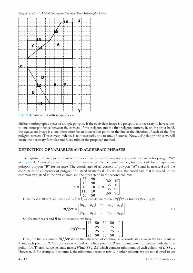
To explain this issue, we can start with an example. We are looking for an equivalent element for polygon “A” in Figure 4. All divisions are 10 mm × 10 mm squares. As mentioned earlier, first, we look for an equivalent polygon, polygon “B” for instance. The coordinates of all corners of polygon “A” stand in matrix 𝐴𝐴 and the coordinates of all corners of polygon “B” stand in matrix 𝐵𝐵. To do this, the coordinate that is related to the common axis, stand in the first column and the other stand in the second column:

𝐴𝐴 =

⎣⎢⎢⎢⎡

35 9010 9010 10

110 1060 50⎦

⎥⎥⎥⎤

,𝐵𝐵 = �

60 1035 1035 9060 90

�

If matrix 𝐴𝐴 is 𝑚𝑚 × 𝑛𝑛 and matrix 𝐵𝐵 is 𝑘𝑘 × 𝑙𝑙, we can define matrix 𝐷𝐷𝐷𝐷𝐷𝐷𝐷𝐷𝐷𝐷𝐷𝐷 as follows (See Eq.1):

𝐷𝐷𝐷𝐷𝐷𝐷𝐷𝐷𝐷𝐷𝐷𝐷 = �|𝑎𝑎11 − 𝑏𝑏11| ⋯ |𝑎𝑎𝑛𝑛1 − 𝑏𝑏11|

⋮ ⋱ ⋮|𝑎𝑎11 − 𝑏𝑏𝑘𝑘1| ⋯ |𝑎𝑎𝑛𝑛1 − 𝑏𝑏𝑘𝑘1|

� (1)

So, for matrices 𝐴𝐴 and 𝐵𝐵 in our example, we have:

𝐷𝐷𝐷𝐷𝐷𝐷𝐷𝐷𝐷𝐷𝐷𝐷 = �

25 50 50 50 00 25 25 75 250 25 25 75 25

25 50 50 50 0

�

Here, the first column of 𝐷𝐷𝐷𝐷𝐷𝐷𝐷𝐷𝐷𝐷𝐷𝐷 shows the difference of common axis coordinate between the first point of 𝐴𝐴 and each point of 𝐵𝐵. Our purpose is to find out which point of 𝐵𝐵 has the minimum difference with the first point of 𝐴𝐴. Therefore, we generate matrix 𝑀𝑀𝐷𝐷𝑛𝑛𝐷𝐷𝐷𝐷𝐷𝐷𝐷𝐷𝐷𝐷𝐷𝐷𝐴𝐴𝐵𝐵 which contains minimums of each column of 𝐷𝐷𝐷𝐷𝐷𝐷𝐷𝐷𝐷𝐷𝐷𝐷. However, if, for example, in column 1, the minimum occurs in row 1, in other columns we are not allowed to get

Figure 4. Sample 2D orthographic view

European Journal of Sustainable Development Research, 3(2), em0081

© 2019 by Author/s 5 / 13

row 1 as the minimum; and if the number of columns is greater than the number of rows for columns that do not have any row to obtain as the minimum, we can get 2×(maximum of matrix 𝐷𝐷𝐷𝐷𝐷𝐷𝐷𝐷𝐷𝐷𝐷𝐷) as the minimum. The reason is that it shows the first polygon has more corners from the second polygon, which is a negative score for their conformity. We call this “the penalty method”. Therefore, in our example, we have:

MinDifferAB = [25 25 25 50 150] Now, if 𝑀𝑀𝐷𝐷𝑛𝑛𝐷𝐷𝐷𝐷𝐷𝐷𝐷𝐷𝐷𝐷𝐷𝐷𝐴𝐴𝐵𝐵 is 1 × 𝑛𝑛, 𝑆𝑆𝑆𝑆𝑚𝑚𝐴𝐴𝐵𝐵 is defined as follows:

𝑆𝑆𝑆𝑆𝑚𝑚𝐴𝐴𝐵𝐵 = �𝑀𝑀𝐷𝐷𝑛𝑛𝐷𝐷𝐷𝐷𝐷𝐷𝐷𝐷𝐷𝐷𝐷𝐷𝐴𝐴𝐵𝐵1𝑖𝑖

𝑛𝑛

𝑖𝑖=1

(2)

which for our example will be: 𝑆𝑆𝑆𝑆𝑚𝑚𝐴𝐴𝐵𝐵 = 25 + 25 + 25 + 50 + 150 = 275.

We then repeat the above process for case 𝐵𝐵𝐴𝐴 (polygon 𝐵𝐵 as the first polygon and polygon 𝐴𝐴 as the equivalent element). So we will have:

𝐷𝐷𝐷𝐷𝐷𝐷𝐷𝐷𝐷𝐷𝐷𝐷 =

⎣⎢⎢⎢⎡25 0 0 2550 25 25 5050 25 25 5050 75 75 500 25 25 0 ⎦

⎥⎥⎥⎤

,𝑀𝑀𝐷𝐷𝑛𝑛𝐷𝐷𝐷𝐷𝐷𝐷𝐷𝐷𝐷𝐷𝐷𝐷𝐵𝐵𝐴𝐴 = [0 0 25 50], 𝑆𝑆𝑆𝑆𝑚𝑚𝐵𝐵𝐴𝐴 = 0 + 0 + 25 + 50 = 75.

Now, if 𝑀𝑀𝐷𝐷𝑛𝑛𝐷𝐷𝐷𝐷𝐷𝐷𝐷𝐷𝐷𝐷𝐷𝐷𝐴𝐴𝐵𝐵 is 1 × 𝑛𝑛 and 𝑀𝑀𝐷𝐷𝑛𝑛𝐷𝐷𝐷𝐷𝐷𝐷𝐷𝐷𝐷𝐷𝐷𝐷𝐵𝐵𝐴𝐴 is 1 × 𝑙𝑙, we define 𝐹𝐹𝐷𝐷𝑛𝑛𝑎𝑎𝑙𝑙𝐷𝐷𝐷𝐷𝐷𝐷𝐷𝐷 as follows:

𝐹𝐹𝐷𝐷𝑛𝑛𝑎𝑎𝑙𝑙𝐷𝐷𝐷𝐷𝐷𝐷𝐷𝐷 =max(𝑆𝑆𝑆𝑆𝑚𝑚𝐴𝐴𝐵𝐵, 𝑆𝑆𝑆𝑆𝑚𝑚𝐵𝐵𝐴𝐴)

max{(𝑛𝑛 × max(𝑀𝑀𝐷𝐷𝑛𝑛𝐷𝐷𝐷𝐷𝐷𝐷𝐷𝐷𝐷𝐷𝐷𝐷𝐴𝐴𝐵𝐵)), (𝑙𝑙 × max(𝑀𝑀𝐷𝐷𝑛𝑛𝐷𝐷𝐷𝐷𝐷𝐷𝐷𝐷𝐷𝐷𝐷𝐷𝐵𝐵𝐴𝐴))} (3)

So, in the mentioned example, we have:

𝐹𝐹𝐷𝐷𝑛𝑛𝑎𝑎𝑙𝑙𝐷𝐷𝐷𝐷𝐷𝐷𝐷𝐷 =max(275,75)

max{(5 × 150), (4 × 75)} =275750

= 0.367

𝐹𝐹𝐷𝐷𝑛𝑛𝑎𝑎𝑙𝑙𝐷𝐷𝐷𝐷𝐷𝐷𝐷𝐷 shows how much difference exists between two polygons after collating the nearest points together, because of the penalty method, the existence of an additional point in each polygon is considered a drawback in 𝐹𝐹𝐷𝐷𝑛𝑛𝑎𝑎𝑙𝑙𝐷𝐷𝐷𝐷𝐷𝐷𝐷𝐷. It is clear that 𝐹𝐹𝐷𝐷𝑛𝑛𝑎𝑎𝑙𝑙𝐷𝐷𝐷𝐷𝐷𝐷𝐷𝐷 is a number between 0 and 1 and if it is near 0, the possibility of conformity between the two polygons is greater. This variable is, therefore, a scale to check the first and second properties mentioned in the surface analysis.

After that, it is necessary to check the third property, i.e. the parallelism of two lines in equivalent polygons. If we show the number of the parallel line pairs of polygon “A” by 𝑃𝑃𝑎𝑎𝐷𝐷𝐴𝐴 and the parallel line pairs of polygon “B” by 𝑃𝑃𝑎𝑎𝐷𝐷𝐵𝐵, 𝑃𝑃𝑎𝑎𝐷𝐷𝐷𝐷𝐷𝐷𝐷𝐷𝐷𝐷 can be defined as follows:

𝑃𝑃𝑎𝑎𝐷𝐷𝐷𝐷𝐷𝐷𝐷𝐷𝐷𝐷 = �|𝑃𝑃𝑎𝑎𝐷𝐷𝐴𝐴 − 𝑃𝑃𝑎𝑎𝐷𝐷𝐵𝐵|

𝑀𝑀𝑎𝑎𝑀𝑀(𝑃𝑃𝑎𝑎𝐷𝐷𝐴𝐴,𝑃𝑃𝑎𝑎𝐷𝐷𝐵𝐵)for max(𝑃𝑃𝑎𝑎𝐷𝐷𝐴𝐴,𝑃𝑃𝑎𝑎𝐷𝐷𝐵𝐵) ≠ 0

0 for max(𝑃𝑃𝑎𝑎𝐷𝐷𝐴𝐴,𝑃𝑃𝑎𝑎𝐷𝐷𝐵𝐵) = 0 (4)

It is clear that, 𝑃𝑃𝑎𝑎𝐷𝐷𝐷𝐷𝐷𝐷𝐷𝐷𝐷𝐷 is a number between 0 and 1 and in case it is closer to 0, it signifies better conformity between the two polygons. In our example, for polygons “A” and “B” we have:

𝑃𝑃𝑎𝑎𝐷𝐷𝐴𝐴 = 1,𝑃𝑃𝑎𝑎𝐷𝐷𝐵𝐵 = 2𝑦𝑦𝑖𝑖𝑦𝑦𝑦𝑦𝑦𝑦𝑦𝑦�⎯⎯⎯� 𝑃𝑃𝑎𝑎𝐷𝐷𝐷𝐷𝐷𝐷𝐷𝐷𝐷𝐷 =

|1 − 2|2

= 0.5 After analyzing the conformity of the two polygons, we then present a method to find out the conformity of

one polygon with a line. This method is greatly similar to the other method with the difference that in matrix 𝐵𝐵, we substitute corners of polygon “B” with the intersection points on the noted line. For example, if we note line 𝐿𝐿1 as the equivalent element for polygon “A”, we will have:

𝐶𝐶 = �110 50110 1060 50

� , 𝐿𝐿1 = �110 9060 903510

9090

�

In ro

w 1

In ro

w 2

In ro

w 3

In ro

w 4

2×M

ax (7

5)

Gorgani et al. / 3D Model Reconstruction from Two Orthographic Views

6 / 13 © 2019 by Author/s

Then, same as the other method, we generate matrix 𝐷𝐷𝐷𝐷𝐷𝐷𝐷𝐷𝐷𝐷𝐷𝐷 as follows:

𝐷𝐷𝐷𝐷𝐷𝐷𝐷𝐷𝐷𝐷𝐷𝐷 = �0 0 50

50 50 075

10075

1002550

�

Now, we generate 𝑀𝑀𝐷𝐷𝑛𝑛𝐷𝐷𝐷𝐷𝐷𝐷𝐷𝐷𝐷𝐷𝐷𝐷𝐴𝐴𝐵𝐵 the same way as the other method but here, recurrence of the rows is permitted. The penalty method, however, is not used here since one intersection point can be equivalent to more than one corner. So, we have:

𝑀𝑀𝐷𝐷𝑛𝑛𝐷𝐷𝐷𝐷𝐷𝐷𝐷𝐷𝐷𝐷𝐷𝐷𝐴𝐴𝐵𝐵 = [0 0 0], 𝑆𝑆𝑆𝑆𝑚𝑚𝐴𝐴𝐵𝐵 = 0 + 0 + 0 = 0 Another difference with the other method is that here we do not perform the reverse process for the line as

the first element and the polygon as the equivalent and 𝑀𝑀𝐷𝐷𝑛𝑛𝐷𝐷𝐷𝐷𝐷𝐷𝐷𝐷𝐷𝐷𝐷𝐷𝐵𝐵𝐴𝐴 is, therefore, not calculated. Hence, if 𝑀𝑀𝐷𝐷𝑛𝑛𝐷𝐷𝐷𝐷𝐷𝐷𝐷𝐷𝐷𝐷𝐷𝐷𝐴𝐴𝐵𝐵 is 1 × 𝑛𝑛, for 𝐹𝐹𝐷𝐷𝑛𝑛𝑎𝑎𝑙𝑙𝐷𝐷𝐷𝐷𝐷𝐷𝐷𝐷 we have:

𝐹𝐹𝐷𝐷𝑛𝑛𝑎𝑎𝑙𝑙𝐷𝐷𝐷𝐷𝐷𝐷𝐷𝐷 = �𝑆𝑆𝑆𝑆𝑚𝑚𝐴𝐴𝐵𝐵

𝑛𝑛 × 𝑀𝑀𝑎𝑎𝑀𝑀(𝑀𝑀𝐷𝐷𝑛𝑛𝐷𝐷𝐷𝐷𝐷𝐷𝐷𝐷𝐷𝐷𝐷𝐷𝐴𝐴𝐵𝐵)for max(𝑀𝑀𝐷𝐷𝑛𝑛𝐷𝐷𝐷𝐷𝐷𝐷𝐷𝐷𝐷𝐷𝐷𝐷𝐴𝐴𝐵𝐵) ≠ 0

0 for max(𝑀𝑀𝐷𝐷𝑛𝑛𝐷𝐷𝐷𝐷𝐷𝐷𝐷𝐷𝐷𝐷𝐷𝐷𝐴𝐴𝐵𝐵) = 0 (5)

So, for polygon 𝐶𝐶 and line 𝐿𝐿1, we have: 𝐹𝐹𝐷𝐷𝑛𝑛𝑎𝑎𝑙𝑙𝐷𝐷𝐷𝐷𝐷𝐷𝐷𝐷 = 0.

As we know from expert knowledge, against each corner of the polygon, there should be an intersection point over the equivalent line. If such a point exists for corner number i, there is a zero in column i of matrix 𝐷𝐷𝐷𝐷𝐷𝐷𝐷𝐷𝐷𝐷𝐷𝐷. So, the number of columns of matrix 𝐷𝐷𝐷𝐷𝐷𝐷𝐷𝐷𝐷𝐷𝐷𝐷 which does not have any zero value is the number of corners of the polygon without any equivalent intersection point over the line. We can define variable 𝑆𝑆𝐷𝐷𝑛𝑛𝑆𝑆𝐶𝐶𝑆𝑆𝐷𝐷 as follows:

𝑆𝑆𝐷𝐷𝑛𝑛𝑆𝑆𝐶𝐶𝑆𝑆𝐷𝐷 =𝑁𝑁𝑆𝑆𝑚𝑚𝑏𝑏𝐷𝐷𝐷𝐷 𝑆𝑆𝐷𝐷 𝑐𝑐𝑆𝑆𝑙𝑙𝑆𝑆𝑚𝑚𝑛𝑛𝑐𝑐 𝑤𝑤𝐷𝐷𝑡𝑡ℎ𝑆𝑆𝑆𝑆𝑡𝑡 𝑧𝑧𝐷𝐷𝐷𝐷𝑆𝑆 𝑣𝑣𝑎𝑎𝑙𝑙𝑆𝑆𝐷𝐷 𝐷𝐷𝑛𝑛 𝑚𝑚𝑎𝑎𝑡𝑡𝐷𝐷𝐷𝐷𝑀𝑀 𝐷𝐷𝐷𝐷𝐷𝐷𝐷𝐷𝐷𝐷𝐷𝐷1

𝑀𝑀𝑎𝑎𝑀𝑀(𝑁𝑁𝑆𝑆𝑚𝑚𝑏𝑏𝐷𝐷𝐷𝐷 𝑆𝑆𝐷𝐷 𝑣𝑣𝐷𝐷𝐷𝐷𝑡𝑡𝐷𝐷𝑐𝑐𝐷𝐷𝑐𝑐 𝑆𝑆𝐷𝐷 𝑝𝑝𝑆𝑆𝑙𝑙𝑝𝑝𝑆𝑆𝑆𝑆𝑛𝑛,𝑁𝑁𝑆𝑆𝑚𝑚𝑏𝑏𝐷𝐷𝐷𝐷 𝑆𝑆𝐷𝐷 𝐷𝐷𝑛𝑛𝑡𝑡𝐷𝐷𝐷𝐷𝑐𝑐𝐷𝐷𝑐𝑐𝑡𝑡𝐷𝐷𝑆𝑆𝑛𝑛 𝑝𝑝𝑆𝑆𝐷𝐷𝑛𝑛𝑡𝑡𝑐𝑐 𝑆𝑆𝑣𝑣𝐷𝐷𝐷𝐷 𝑙𝑙𝐷𝐷𝑛𝑛𝐷𝐷) (6)

So in our example for polygon 𝐶𝐶 and line 𝐿𝐿1 we have:

𝑆𝑆𝐷𝐷𝑛𝑛𝑆𝑆𝐶𝐶𝑆𝑆𝐷𝐷 =04

= 0. It is clear that 𝑆𝑆𝐷𝐷𝑛𝑛𝑆𝑆𝐶𝐶𝑆𝑆𝐷𝐷 is a number between 0 and 1 and in case it is closer to 0, the conformity of the polygon

and the line is better.

FUZZY VARIABLES AND MEMBERSHIP FUNCTIONS

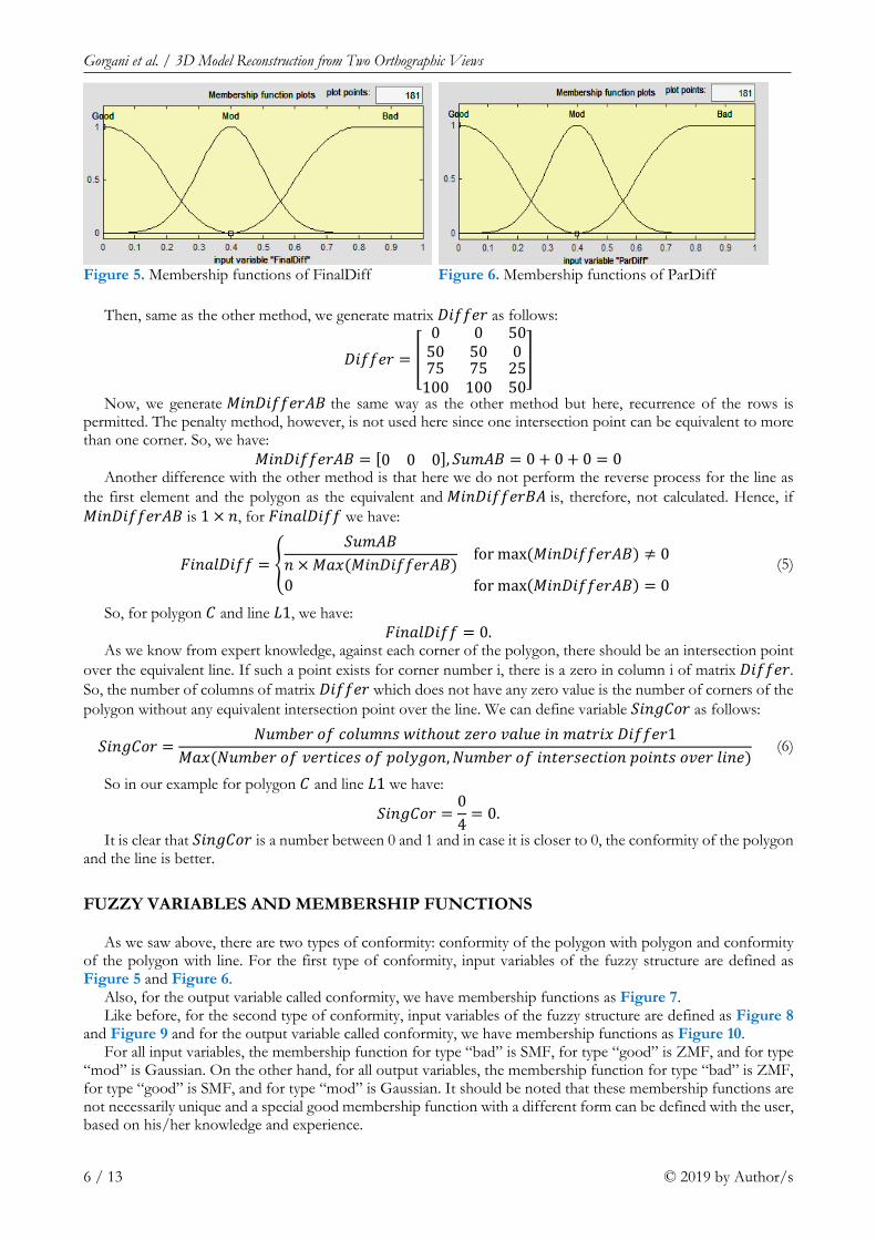
As we saw above, there are two types of conformity: conformity of the polygon with polygon and conformity of the polygon with line. For the first type of conformity, input variables of the fuzzy structure are defined as Figure 5 and Figure 6.

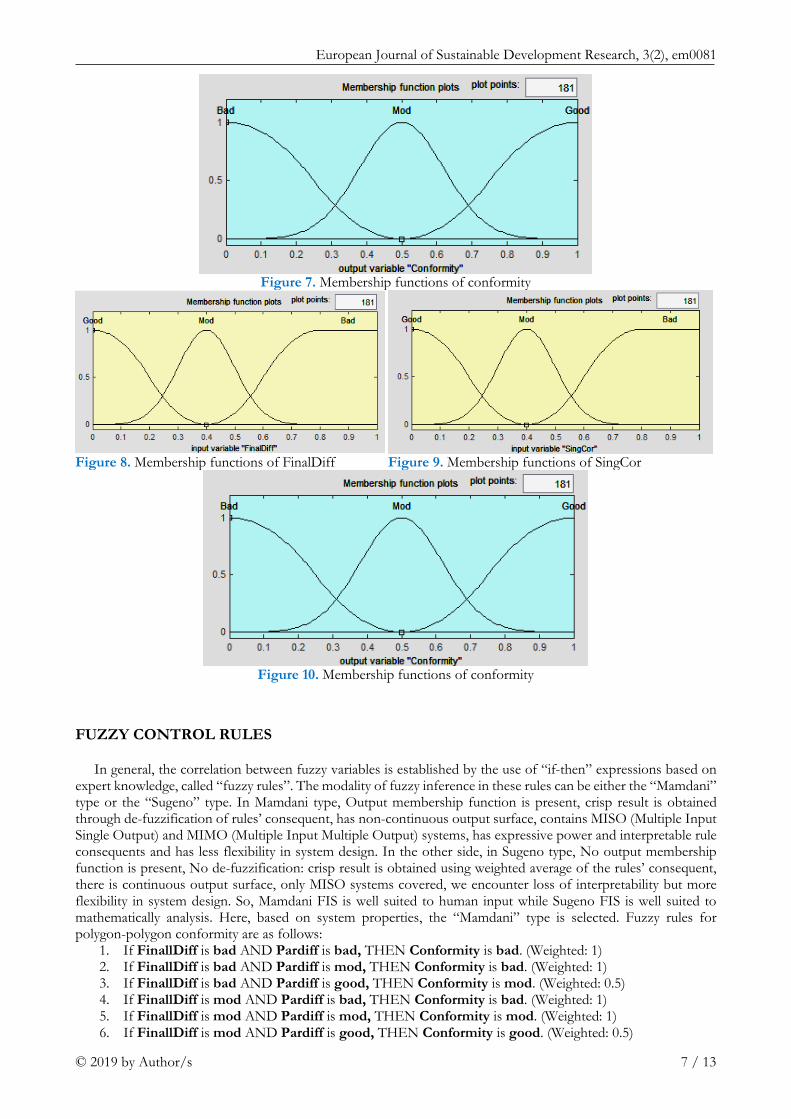
Also, for the output variable called conformity, we have membership functions as Figure 7. Like before, for the second type of conformity, input variables of the fuzzy structure are defined as Figure 8

and Figure 9 and for the output variable called conformity, we have membership functions as Figure 10. For all input variables, the membership function for type “bad” is SMF, for type “good” is ZMF, and for type

“mod” is Gaussian. On the other hand, for all output variables, the membership function for type “bad” is ZMF, for type “good” is SMF, and for type “mod” is Gaussian. It should be noted that these membership functions are not necessarily unique and a special good membership function with a different form can be defined with the user, based on his/her knowledge and experience.

Figure 5. Membership functions of FinalDiff Figure 6. Membership functions of ParDiff

European Journal of Sustainable Development Research, 3(2), em0081

© 2019 by Author/s 7 / 13

FUZZY CONTROL RULES

In general, the correlation between fuzzy variables is established by the use of “if-then” expressions based on expert knowledge, called “fuzzy rules”. The modality of fuzzy inference in these rules can be either the “Mamdani” type or the “Sugeno” type. In Mamdani type, Output membership function is present, crisp result is obtained through de-fuzzification of rules’ consequent, has non-continuous output surface, contains MISO (Multiple Input Single Output) and MIMO (Multiple Input Multiple Output) systems, has expressive power and interpretable rule consequents and has less flexibility in system design. In the other side, in Sugeno type, No output membership function is present, No de-fuzzification: crisp result is obtained using weighted average of the rules’ consequent, there is continuous output surface, only MISO systems covered, we encounter loss of interpretability but more flexibility in system design. So, Mamdani FIS is well suited to human input while Sugeno FIS is well suited to mathematically analysis. Here, based on system properties, the “Mamdani” type is selected. Fuzzy rules for polygon-polygon conformity are as follows:

1. If FinallDiff is bad AND Pardiff is bad, THEN Conformity is bad. (Weighted: 1) 2. If FinallDiff is bad AND Pardiff is mod, THEN Conformity is bad. (Weighted: 1) 3. If FinallDiff is bad AND Pardiff is good, THEN Conformity is mod. (Weighted: 0.5) 4. If FinallDiff is mod AND Pardiff is bad, THEN Conformity is bad. (Weighted: 1) 5. If FinallDiff is mod AND Pardiff is mod, THEN Conformity is mod. (Weighted: 1) 6. If FinallDiff is mod AND Pardiff is good, THEN Conformity is good. (Weighted: 0.5)

Figure 7. Membership functions of conformity

Figure 8. Membership functions of FinalDiff Figure 9. Membership functions of SingCor

Figure 10. Membership functions of conformity

Gorgani et al. / 3D Model Reconstruction from Two Orthographic Views

8 / 13 © 2019 by Author/s

7. If FinallDiff is good AND Pardiff is bad, THEN Conformity is bad. (Weighted: 0.5) 8. If FinallDiff is good AND Pardiff is mod, THEN Conformity is mod. (Weighted: 0.5) 9. If FinallDiff is good AND Pardiff is good, THEN Conformity is good. (Weighted: 1)

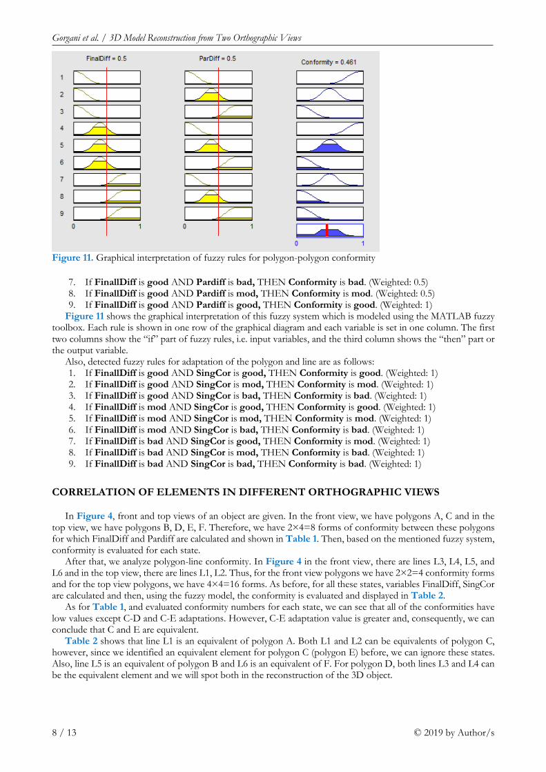
Figure 11 shows the graphical interpretation of this fuzzy system which is modeled using the MATLAB fuzzy toolbox. Each rule is shown in one row of the graphical diagram and each variable is set in one column. The first two columns show the “if” part of fuzzy rules, i.e. input variables, and the third column shows the “then” part or the output variable.

Also, detected fuzzy rules for adaptation of the polygon and line are as follows: 1. If FinallDiff is good AND SingCor is good, THEN Conformity is good. (Weighted: 1) 2. If FinallDiff is good AND SingCor is mod, THEN Conformity is mod. (Weighted: 1) 3. If FinallDiff is good AND SingCor is bad, THEN Conformity is bad. (Weighted: 1) 4. If FinallDiff is mod AND SingCor is good, THEN Conformity is good. (Weighted: 1) 5. If FinallDiff is mod AND SingCor is mod, THEN Conformity is mod. (Weighted: 1) 6. If FinallDiff is mod AND SingCor is bad, THEN Conformity is bad. (Weighted: 1) 7. If FinallDiff is bad AND SingCor is good, THEN Conformity is mod. (Weighted: 1) 8. If FinallDiff is bad AND SingCor is mod, THEN Conformity is bad. (Weighted: 1) 9. If FinallDiff is bad AND SingCor is bad, THEN Conformity is bad. (Weighted: 1)

CORRELATION OF ELEMENTS IN DIFFERENT ORTHOGRAPHIC VIEWS

In Figure 4, front and top views of an object are given. In the front view, we have polygons A, C and in the top view, we have polygons B, D, E, F. Therefore, we have 2×4=8 forms of conformity between these polygons for which FinalDiff and Pardiff are calculated and shown in Table 1. Then, based on the mentioned fuzzy system, conformity is evaluated for each state.

After that, we analyze polygon-line conformity. In Figure 4 in the front view, there are lines L3, L4, L5, and L6 and in the top view, there are lines L1, L2. Thus, for the front view polygons we have 2×2=4 conformity forms and for the top view polygons, we have 4×4=16 forms. As before, for all these states, variables FinalDiff, SingCor are calculated and then, using the fuzzy model, the conformity is evaluated and displayed in Table 2.

As for Table 1, and evaluated conformity numbers for each state, we can see that all of the conformities have low values except C-D and C-E adaptations. However, C-E adaptation value is greater and, consequently, we can conclude that C and E are equivalent.

Table 2 shows that line L1 is an equivalent of polygon A. Both L1 and L2 can be equivalents of polygon C, however, since we identified an equivalent element for polygon C (polygon E) before, we can ignore these states. Also, line L5 is an equivalent of polygon B and L6 is an equivalent of F. For polygon D, both lines L3 and L4 can be the equivalent element and we will spot both in the reconstruction of the 3D object.

Figure 11. Graphical interpretation of fuzzy rules for polygon-polygon conformity

European Journal of Sustainable Development Research, 3(2), em0081

© 2019 by Author/s 9 / 13

RECONSTRUCTION OF THE 3D OBJECT

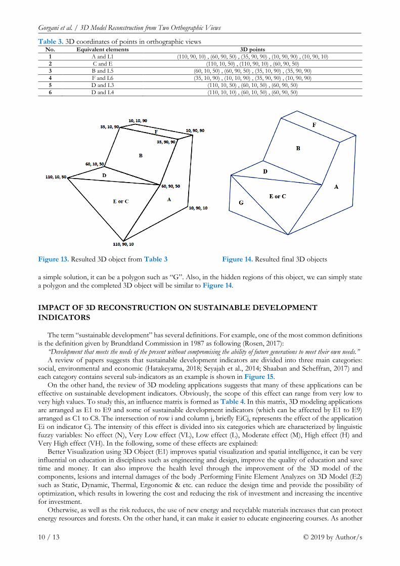
Based on the results of Tables 1 and 2 and as the x-axis is the common axis between the two views, it is sufficient to collate points in equivalent elements and obtain 3D coordinates of each point. Results are shown in Table 3.

Now, we locate the points of Table 3 in the 3D state. Figure 13 is obtained. The lower left corner of the 3D object is empty and based on the two given orthographic views, the noted region is a straight line in views, so, as

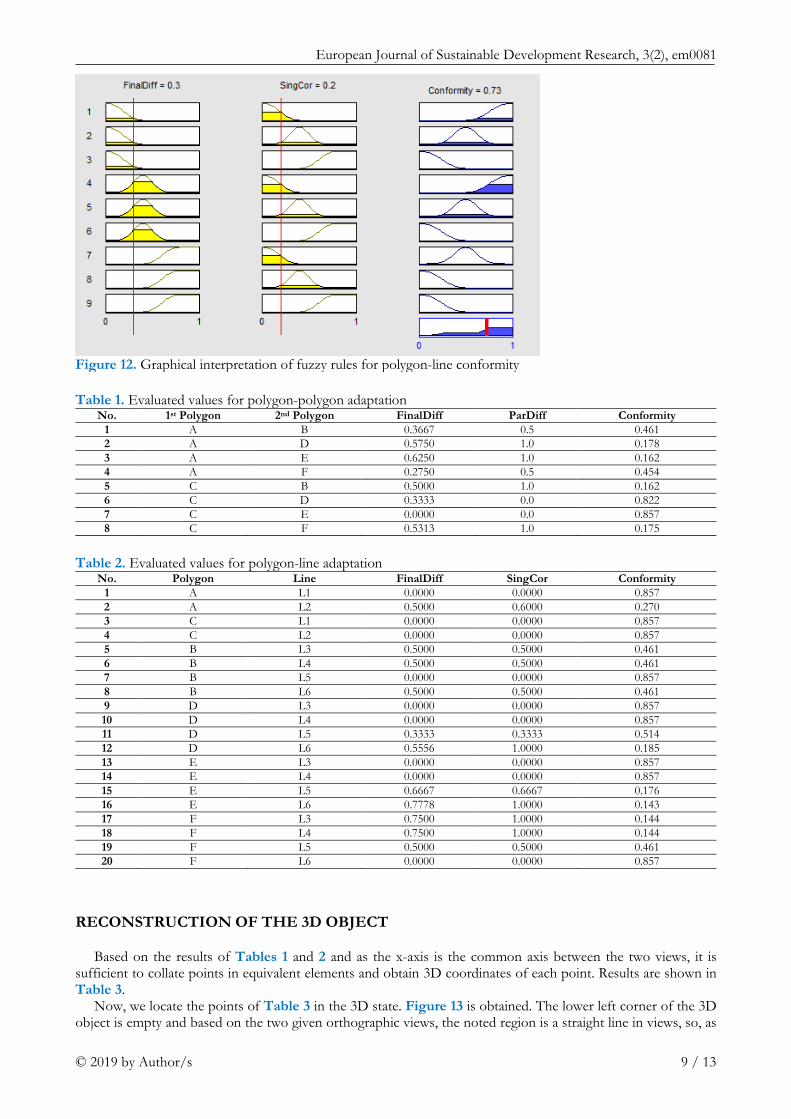
Figure 12. Graphical interpretation of fuzzy rules for polygon-line conformity

Table 1. Evaluated values for polygon-polygon adaptation No. 1st Polygon 2nd Polygon FinalDiff ParDiff Conformity

1 A B 0.3667 0.5 0.461 2 A D 0.5750 1.0 0.178 3 A E 0.6250 1.0 0.162 4 A F 0.2750 0.5 0.454 5 C B 0.5000 1.0 0.162 6 C D 0.3333 0.0 0.822 7 C E 0.0000 0.0 0.857 8 C F 0.5313 1.0 0.175

Table 2. Evaluated values for polygon-line adaptation No. Polygon Line FinalDiff SingCor Conformity

1 A L1 0.0000 0.0000 0.857 2 A L2 0.5000 0.6000 0.270 3 C L1 0.0000 0.0000 0.857 4 C L2 0.0000 0.0000 0.857 5 B L3 0.5000 0.5000 0.461 6 B L4 0.5000 0.5000 0.461 7 B L5 0.0000 0.0000 0.857 8 B L6 0.5000 0.5000 0.461 9 D L3 0.0000 0.0000 0.857 10 D L4 0.0000 0.0000 0.857 11 D L5 0.3333 0.3333 0.514 12 D L6 0.5556 1.0000 0.185 13 E L3 0.0000 0.0000 0.857 14 E L4 0.0000 0.0000 0.857 15 E L5 0.6667 0.6667 0.176 16 E L6 0.7778 1.0000 0.143 17 F L3 0.7500 1.0000 0.144 18 F L4 0.7500 1.0000 0.144 19 F L5 0.5000 0.5000 0.461 20 F L6 0.0000 0.0000 0.857

Gorgani et al. / 3D Model Reconstruction from Two Orthographic Views

10 / 13 © 2019 by Author/s

a simple solution, it can be a polygon such as “G”. Also, in the hidden regions of this object, we can simply state a polygon and the completed 3D object will be similar to Figure 14.

IMPACT OF 3D RECONSTRUCTION ON SUSTAINABLE DEVELOPMENT INDICATORS

The term “sustainable development” has several definitions. For example, one of the most common definitions is the definition given by Brundtland Commission in 1987 as following (Rosen, 2017):

“Development that meets the needs of the present without compromising the ability of future generations to meet their own needs.” A review of papers suggests that sustainable development indicators are divided into three main categories:

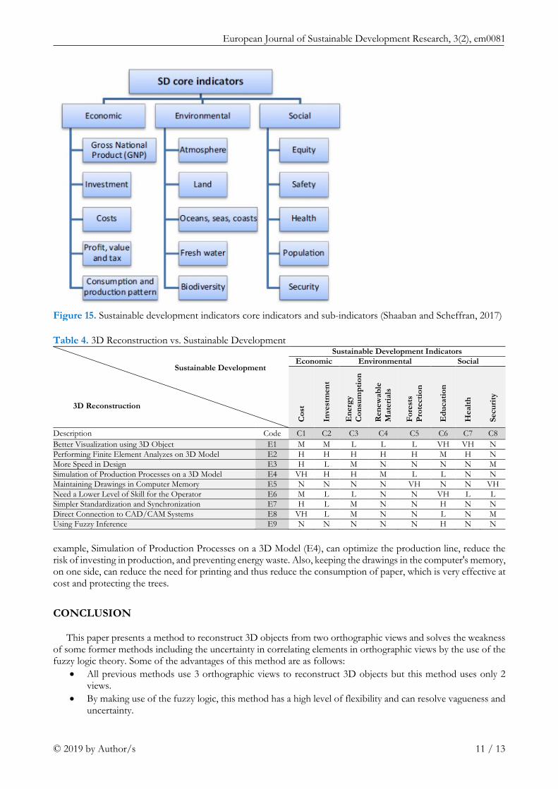
social, environmental and economic (Hatakeyama, 2018; Seyajah et al., 2014; Shaaban and Scheffran, 2017) and each category contains several sub-indicators as an example is shown in Figure 15.

On the other hand, the review of 3D modeling applications suggests that many of these applications can be effective on sustainable development indicators. Obviously, the scope of this effect can range from very low to very high values. To study this, an influence matrix is formed as Table 4. In this matrix, 3D modeling applications are arranged as E1 to E9 and some of sustainable development indicators (which can be affected by E1 to E9) arranged as C1 to C8. The intersection of row i and column j, briefly EiCj, represents the effect of the application Ei on indicator Cj. The intensity of this effect is divided into six categories which are characterized by linguistic fuzzy variables: No effect (N), Very Low effect (VL), Low effect (L), Moderate effect (M), High effect (H) and Very High effect (VH). In the following, some of these effects are explained:

Better Visualization using 3D Object (E1) improves spatial visualization and spatial intelligence, it can be very influential on education in disciplines such as engineering and design, improve the quality of education and save time and money. It can also improve the health level through the improvement of the 3D model of the components, lesions and internal damages of the body .Performing Finite Element Analyzes on 3D Model (E2) such as Static, Dynamic, Thermal, Ergonomic & etc. can reduce the design time and provide the possibility of optimization, which results in lowering the cost and reducing the risk of investment and increasing the incentive for investment.

Otherwise, as well as the risk reduces, the use of new energy and recyclable materials increases that can protect energy resources and forests. On the other hand, it can make it easier to educate engineering courses. As another

Table 3. 3D coordinates of points in orthographic views No. Equivalent elements 3D points

1 A and L1 (110, 90, 10) , (60, 90, 50) , (35, 90, 90) , (10, 90, 90) , (10, 90, 10) 2 C and E (110, 10, 50) , (110, 90, 10) , (60, 90, 50) 3 B and L5 (60, 10, 50) , (60, 90, 50) , (35, 10, 90) , (35, 90, 90) 4 F and L6 (35, 10, 90) , (10, 10, 90) , (35, 90, 90) , (10, 90, 90) 5 D and L3 (110, 10, 50) , (60, 10, 50) , (60, 90, 50) 6 D and L4 (110, 10, 10) , (60, 10, 50) , (60, 90, 50)

Figure 13. Resulted 3D object from Table 3 Figure 14. Resulted final 3D objects

European Journal of Sustainable Development Research, 3(2), em0081

© 2019 by Author/s 11 / 13

example, Simulation of Production Processes on a 3D Model (E4), can optimize the production line, reduce the risk of investing in production, and preventing energy waste. Also, keeping the drawings in the computer's memory, on one side, can reduce the need for printing and thus reduce the consumption of paper, which is very effective at cost and protecting the trees.

CONCLUSION

This paper presents a method to reconstruct 3D objects from two orthographic views and solves the weakness of some former methods including the uncertainty in correlating elements in orthographic views by the use of the fuzzy logic theory. Some of the advantages of this method are as follows:

• All previous methods use 3 orthographic views to reconstruct 3D objects but this method uses only 2 views.

• By making use of the fuzzy logic, this method has a high level of flexibility and can resolve vagueness and uncertainty.

Figure 15. Sustainable development indicators core indicators and sub-indicators (Shaaban and Scheffran, 2017)

Table 4. 3D Reconstruction vs. Sustainable Development

Sustainable Development

3D Reconstruction

Sustainable Development Indicators Economic Environmental Social

Cos

t

Inve

stm

ent

Ene

rgy

Con

sum

ptio

n

Ren

ewab

le

Mat

eria

ls

Fore

sts

Prot

ectio

n

Edu

catio

n

Hea

lth

Secu

rity

Description Code C1 C2 C3 C4 C5 C6 C7 C8 Better Visualization using 3D Object E1 M M L L L VH VH N Performing Finite Element Analyzes on 3D Model E2 H H H H H M H N More Speed in Design E3 H L M N N N N M Simulation of Production Processes on a 3D Model E4 VH H H M L L N N Maintaining Drawings in Computer Memory E5 N N N N VH N N VH Need a Lower Level of Skill for the Operator E6 M L L N N VH L L Simpler Standardization and Synchronization E7 H L M N N H N N Direct Connection to CAD/CAM Systems E8 VH L M N N L N M Using Fuzzy Inference E9 N N N N N H N N

Gorgani et al. / 3D Model Reconstruction from Two Orthographic Views

12 / 13 © 2019 by Author/s

• This method is based on expert knowledge, so there is very low possibility of the absolutism of computer systems.

• Since this method presents different possibilities for each adaptation state, it can be used to reconstruct final 3D objects of scratched engineering drawings.

Meanwhile, a limitation of this method is that it can only be applied to planar faces and does not include curved surfaces. In future research, it is suggested that its scope should be broadened to involve curved surfaces.

On the other hand, increasing the possibility of reconstruction of 3D Objects from 2D orthographic views will result lower cost, lower investment risk, reduced energy consumption, increased use of renewable materials, conservation of natural resources, improved education quality and increased health level, all of which means creating sustainable development in three areas: economic, social, and environmental.

REFERENCES

Aldefeld, B. (1983). On automatic recognition of 3D structures from 2D representations. Computer-Aided Design, 15(2), 59-64. https://doi.org/10.1016/0010-4485(83)90169-0

Bai, J., Gao, S., Tang, W., Liu, Y. and Guo, S. (2010). Design reuse oriented partial retrieval of CAD models. Computer-Aided Design, 42(12), 1069-1084. https://doi.org/10.1016/j.cad.2010.07.002

Banapurmath, N., Gadwal, S., Kamoji, M., Rampure, P. and Khandal, S. (2018). Impact of Injection Timing on the Performance of Single Cylinder DI Diesel Engine Fueled with Solid Waste Converted Fuel. European Journal of Sustainable Development Research, 2(4), 39. https://doi.org/10.20897/ejosdr/3914

Bezdek, J. (1994). Fuzziness vs. probability-again (!?). IEEE Transactions on Fuzzy systems, 2(1), 1-3. Biasotti, S., Cerri, A., Bronstein, A. and Bronstein, M. (2016). Recent trends, applications, and perspectives in 3D shape

similarity assessment. Paper presented at the Computer Graphics Forum. https://doi.org/10.1111/cgf.12734 Dubois, D. and Prade, H. (1993). Fuzzy sets and probability: misunderstandings, bridges and gaps. Paper presented at the

Second IEEE International Conference on Fuzzy Systems. https://doi.org/10.1109/FUZZY.1993.327367 Elnashaie, S., Danafar, F. and Abashar, M. (2018). Maximum Production Minimum Pollution (MPMP), Necessary

but not Sufficient for Sustainability. European Journal of Sustainable Development Research, 2(4), 41. https://doi.org/10.20897/ejosdr/3909

Geng, W., Wang, J. and Zhang, Y. (2002). Embedding visual cognition in 3D reconstruction from multi-view engineering drawings. Computer-Aided Design, 34(4), 321-336. https://doi.org/10.1016/S0010-4485(01)00092-6

Gorgani, H. H. (2016a). Improvements in Teaching Projection Theory Using Failure Mode and Effects Analysis (FMEA). Journal of Engineering and Applied Sciences, 100(1), 37-42.

Gorgani, H. H. (2016b). Innovative conceptual design on a tracked robot using TRIZ method for passing narrow obstacles. Indian Journal of Science and Technology, 9(7). https://doi.org/10.17485/ijst/2016/v9i7/87857

Gorgani, H. H., Neyestanaki, I. M. S. and Pak, A. J. (2017). Solid Reconstruction from Two Orthographic Views Using Extrusion and Comparative Projections. Journal of Engineering and Applied Sciences, 12(7), 1938-1945.

Haghshenas Gorgani, H. and Jahantigh Pak, A. (2018). A Genetic Algorithm based Optimization Method in 3D Solid Reconstruction from 2D Multi-View Engineering Drawings. Journal of Computational Applied Mechanics, 49(1), 161-170. https://doi.org/10.22059/jcamech.2018.249623.229

Haghshenas Gorgani, H., Maghsoudi, P. and Sadeghi, S. (2018). An Innovative Approach for Study of Thermal Behavior of an Unsteady Nanofluid Squeezing Flow between Two Parallel Plates Utilizing Artificial Neural Network. European Journal of Sustainable Development Research. https://doi.org/10.20897/ejosdr/3935

Hatakeyama, T. (2018). Sustainable development indicators: Conceptual frameworks of comparative indicators sets for local administrations in Japan. Sustainable Development. https://doi.org/10.1002/sd.1738

Jeon, S. M., Lee, J. H., Hahm, G. J. and Suh, H. W. (2016). Automatic CAD model retrieval based on design documents using semantic processing and rule processing. Computers in Industry, 77, 29-47. https://doi.org/10.1016/j.compind.2016.01.002

Jiang, S.-P. and Fu, Z.-G. (2011). Preprocessing for solid reconstruction from engineering drawing. Paper presented at the IEEE International Conference on Computer Science and Automation Engineering (CSAE).

Jianu, O. and Rosen, M. A. (2017). Preliminary Assessment of Noise Pollution Prevention in Wind Turbines Based on an Exergy Approach. European Journal of Sustainable Development Research, 1(2), 12. https://doi.org/10.20897/ejosdr.201712

Lahner, Z., Rodola, E., Schmidt, F. R., Bronstein, M. M. and Cremers, D. (2016). Efficient globally optimal 2d-to-3d deformable shape matching. Paper presented at the Proceedings of the IEEE Conference on Computer Vision and Pattern Recognition. https://doi.org/10.1109/CVPR.2016.240

Lee, H. and Han, S. (2005). Reconstruction of 3D interacting solids of revolution from 2D orthographic views. Computer-Aided Design, 37(13), 1388-1398. https://doi.org/10.1016/j.cad.2005.01.007

European Journal of Sustainable Development Research, 3(2), em0081

© 2019 by Author/s 13 / 13

López-Sastre, R. J., García-Fuertes, A., Redondo-Cabrera, C., Acevedo-Rodríguez, F. J. and Maldonado-Bascón, S. (2013). Evaluating 3d spatial pyramids for classifying 3d shapes. Computers & Graphics, 37(5), 473-483. https://doi.org/10.1016/j.cag.2013.04.003

Mottaghipour, A., Mottaghipour, M., Moradi, D. and Mottaghipour, M. (2018). Fundamentals of Engieering Drawing 2 (1 ed.): Sharif CAD/CAM.

Mottaghipour, M., Hamidi, S., Shirdel, H. R. and Mottaghipour, M. (2017). Fundamentals of Engineering Drawing 1 (4 ed.): Sharif CAD/CAM.

Mura, C., Mattausch, O. and Pajarola, R. (2016). Piecewise‐planar Reconstruction of Multi‐room Interiors with Arbitrary Wall Arrangements. Paper presented at the Computer Graphics Forum. https://doi.org/10.1111/cgf.13015

Mura, C., Mattausch, O., Villanueva, A. J., Gobbetti, E. and Pajarola, R. (2014). Automatic room detection and reconstruction in cluttered indoor environments with complex room layouts. Computers & Graphics, 44, 20-32. https://doi.org/10.1016/j.cag.2014.07.005

Ochmann, S., Vock, R., Wessel, R. and Klein, R. (2016). Automatic reconstruction of parametric building models from indoor point clouds. Computers & Graphics, 54, 94-103. https://doi.org/10.1016/j.cag.2015.07.008

Rosen, M. A. (2017). Sustainable Development: A Vital Quest. European Journal of Sustainable Development Research, 1(1), 2. https://doi.org/10.20897/ejosdr.201702

Ross, T. J. (2009). Fuzzy logic with engineering applications: John Wiley & Sons. Sakurai, H. and Gossard, D. C. (1983). Solid model input through orthographic views (Vol. 17): ACM.

https://doi.org/10.1145/800059.801155 Seyajah, N., Cheng, K. and Bateman, R. (2014). Development of Sustainable Design Index for Office Furniture Design and

its CAD-Based Implementation. Paper presented at the ASME 2014 International Design Engineering Technical Conferences and Computers and Information in Engineering Conference. https://doi.org/10.1115/DETC2014-35642

Shaaban, M. and Scheffran, J. (2017). Selection of sustainable development indicators for the assessment of electricity production in Egypt, 22, 65-73.

Shahriari, G., Maghsoudi, P. and Sadeghi, S. (2018). Impact of Viscous Dissipation on Temperature Distribution of a Two-dimensional Unsteady Graphene Oxide Nanofluid Flow between Two Moving Parallel Plates Employing Akbari-Ganji Method. European Journal of Sustainable Development Research, 2(2), 24. https://doi.org/10.20897/ejosdr/81574

Shin, B.-S. and Shin, Y. G. (1998). Fast 3D solid model reconstruction from orthographic views. Computer-Aided Design, 30(1), 63-76. https://doi.org/10.1016/S0010-4485(97)00054-7

Soni, S. and Gurumoorthy, B. (2003). Handling solids of revolution in volume-based construction of solid models from orthographic views. Journal of Computing and Information Science in Engineering, 3(3), 250-259. https://doi.org/10.1115/1.1604831

Stephan, M. and Cordy, J. R. (2013). A Survey of Model Comparison Approaches and Applications. Paper presented at the Modelsward.

Su, Z., Zhou, L., Li, W., Dai, Y. and Tang, W. (2013). Topology authentication for CAPD models based on Laplacian coordinates. Computers & Graphics, 37(4), 269-279. https://doi.org/10.1016/j.cag.2013.02.009

Wang, M., Gao, Y., Lu, K. and Rui, Y. (2013). View-based discriminative probabilistic modeling for 3D object retrieval and recognition. IEEE Transactions on Image Processing, 22(4), 1395-1407. https://doi.org/10.1109/TIP.2012.2231088

Wang, W. and Grinstein, G. G. (1993). A survey of 3D solid reconstruction from 2D projection line drawings. Paper presented at the Computer Graphics Forum. https://doi.org/10.1111/1467-8659.1220137

Wang, Z. and Latif, M. (2007). Reconstruction of 3D Solid Models Using Fuzzy Logic Recognition. Paper presented at the World Congress on Engineering.

Wen, R., Tang, W. and Su, Z. (2015). A 2D Engineering Drawing and 3D Model Matching Algorithm for Process Plant. Paper presented at the International Conference on the Virtual Reality and Visualization (ICVRV). https://doi.org/10.1111/1467-8659.1220137

Wen, R., Tang, W. and Su, Z. (2017a). Measuring 3D process plant model similarity based on topological relationship distribution. Computer-Aided Design and Applications, 14(4), 422-435. https://doi.org/10.1080/16864360.2016.1257185

Wen, R., Tang, W. and Su, Z. (2017b). Topology based 2D engineering drawing and 3D model matching for process plant. Graphical Models, 92, 1-15. https://doi.org/10.1016/j.gmod.2017.06.001

Zadeh, L. A. (1965). Fuzzy sets. Information and control, 8(3), 338-353. https://doi.org/10.1016/S0019-9958(65)90241-X