3D Mobile-to-Mobile Wireless Channel Model

Prasad T. Samarasinghe, Tharaka A. Lamahewa, Thushara D. Abhayapala and Rodney A. KennedyApplied Signal Processing Group,

Research School of Information Sciences and Engineering,

ANU College of Engineering and Computer Science,

The Australian National University,

Canberra ACT 0200, Australia

{prasad.samarasinghe,tharaka.lamahewa,thushara.abhayapala,rodney.kennedy}@anu.edu.au

Abstract—A three-dimensional single-input single-outputMobile-to-Mobile wireless channel model is developed in thispaper by considering the underlying physics of free spacewave propagation. Based on this channel model, the temporalcorrelation function for a general three dimensional scatteringenvironment is derived. The temporal correlation function ischaracterized by the joint angular power distribution at thetransmitter and receiver antennas and the speed of transmitterand receiver antennas. Using a von Mises-Fisher distribution asthe angular power distribution, the usefulness of the derivedtemporal correlation function is discussed.

I. INTRODUCTION

A communication system in which both the transmitterand receiver are in motion, can be called as a Mobile-to-Mobile (M2M) communication system. The main applicationsof M2M systems are in mobile ad-hoc wireless networks andintelligent transport systems. Dedicated Short Range Commu-nication (DSRC) and Wireless Access in a Vehicular Environ-ment (WAVE) are emerging standards for intelligent transportsystems focussed on improving traveler safety, efficiency andproductivity [1]. Understanding of M2M wireless channel andits behavior will support to improve the above applications.

In the literature, M2M channels have been modeled invarious ways. Akki and Harber [2, 3] were the first to pro-pose a statistical channel model for single-input single-output(SISO) M2M Rayleigh fading radio channel under non line ofsight conditions. Simulation methods for SISO M2M channelshave been proposed in [4–6]. Also, Patzold in [7] deriveda two-dimensional(2D) ray-tracing model for multiple-inputmultiple-output (MIMO) M2M narrowband channel by con-sidering a geometrical two-ring scattering model. Stuber in [8]proposed a similar 2D ray-tracing narrowband channel modelfor MIMO M2M channel based on ‘double-ring’ geometricalmodel. However, since the latter model is independent of thedistances between scatters and antenna elements, it is betterthan the former model. In [9] the narrowband channel modelproposed in [10] was extended to a 2D wideband model.In [11] and [12] these two 2D M2M channels models wereextended to 3D models by assuming scatterers are placed oncylinders. One shortcoming of these ray-tracing geometricalbased channel models is that they cannot be utilized torepresent general scattering scenarios.

In this paper we introduce a novel three-dimensional (3D)M2M channel model based on free-space wave propagationwhere the scattering environment surrounding the transmitterand the receiver is characterized using a random scatteringgain, which is a function of angle of departure (AOD) andangle of arrival (AOA). When compared with other modelsdiscussed above, this channel model can be used for any3D scattering environment whereas the other models arerestricted. Based on this channel model we derive the temporalcorrelation function for a general 3D scattering environment.The temporal correlation function is characterized by thejoint angular power distribution at the transmitter and receiverantennas and the speed of transmitter and receiver antennas.As a special case, in this paper we consider separable scat-tering environments, i.e., the angular power distribution at thereceiver is independent of that at the transmitter. In this case,using the von Mises-Fisher distribution as an example for theangular power distribution at each end of the channel, wecalculate the temporal correlation function for several fadingscenarios and discuss the usefulness of our proposed model.

The rest of the paper is organized as follows. In Section II,we present our new 3D M2M channel model. Using this chan-nel model, in Section III we derive the temporal correlationcorresponding to a general scattering environment. In SectionIV we provide numerical examples to show the strength of theproposed model. Finally, the concluding remarks are given inSection V.

Notations: Throughout the paper, the following notationswill be used: bold lower letters denote vectors, a unit vectoris represented by x and (·)∗ denotes the complex conjugateoperation. The symbol δ(·) denotes the Dirac delta functionwhile E {·} denotes the mathematical expectation. The scalarproduct between vectors x and y is denoted by x · y andi =

√−1.

II. MOBILE-TO-MOBILE CHANNEL MODEL

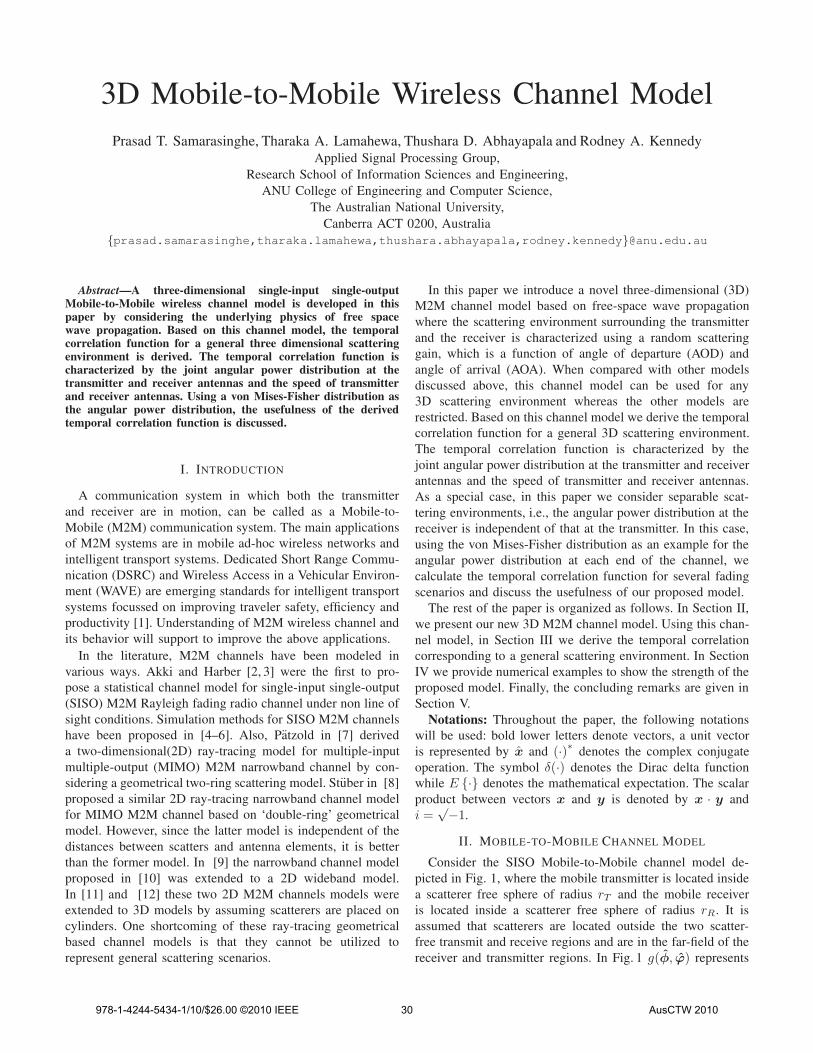
Consider the SISO Mobile-to-Mobile channel model de-picted in Fig. 1, where the mobile transmitter is located insidea scatterer free sphere of radius rT and the mobile receiveris located inside a scatterer free sphere of radius rR. It isassumed that scatterers are located outside the two scatter-free transmit and receive regions and are in the far-field of thereceiver and transmitter regions. In Fig. 1 g(φ, ϕ) represents

AusCTW 2010978-1-4244-5434-1/10/$26.00 ©2010 IEEE 30

)

ϕ

φ

g(φ,ϕ

(a)

(b)

(c)

^

^^

^

v

u

Scatterers

Receiver

Transmitter

Fig. 1. A general scattering model for a flat fading M2M wirelesscommunication system

the effective random complex scattering gain function for asignal leaving the transmitter scatter-free region at a directionφ (relative to the transmitter region origin) and entering thereceiver scatter-free region from a direction ϕ (relative to thereceiver region origin). Suppose the transmitter is moving atconstant velocity u in the direction of u and the receiver ismoving at constant velocity v in the direction of v. Followingthe derivation of fixed-to-mobile channel model given in [13],the signal received at the mobile receiver at time t can bewritten as

y(t) =

∫∫

S×S

x(t)g(φ, ϕ)e−iktuu·φeiktvv·ϕdφdϕ + n(t),

(1)

where x(t) is the baseband transmitted signal, k = 2π/λ is thewave number with λ being the wavelength, n(t) is the additivenoise at the receiver. The integration in (1) above is over aunit circle for a two dimensional scattering (or multipath)environment or over a unit sphere for a three dimensionalscattering environment.

The input-output relationship for the general case then canbe written as

y(t) = h(t)x(t) + n(t) (2)

where, comparing (1) and (2), the underlying time-varyingfading channel between the receiver and the transmitter canbe written as,

h(t) =

∫∫

S×S

g(φ, ϕ)e−iktuu·φeiktvv·ϕdφdϕ. (3)

The channel temporal correlation, which is the correlationbetween the channel gain at time t and time t− τ can then befound from

ρ(τ) ! E {h(t)h∗(t − τ)} .

=

∫

4E

{

g(φ, ϕ)g∗(φ′, ϕ′)}

eiku(−tu·φ+(t−τ)u·φ′)

×e−ikv(−tv·ϕ+(t−τ)v·ϕ′)dφdϕdφ′dϕ′, (4)

where we have introduced the shorthand∫

4 !∫∫

S×S

∫∫

S×S. In

this work we assume that the scattering environment is wide-sense stationary zero-mean and uncorrelated. Therefore, thesecond-order statistics of the scattering gain function g(φ, ϕ)can be written as [14]

E{

g(φ, ϕ)g∗(φ′, ϕ′)}

! G(φ, ϕ)δ(φ − φ′)δ(ϕ − ϕ′),

where G(φ, ϕ) = E{

|g(φ, ϕ)|2}

characterizes the joint

power spectral density (PSD) or the joint angular powerdistribution surrounding the transmitter and receiver regions.In this case the temporal correlation function in (4) furthersimplifies to

ρ(τ) =

∫∫

S×S

G(φ, ϕ)e−ikuτ u·φeikvτ v·ϕdφdϕ. (5)

From (5) above it can be seen that the temporal correlationfunction of a mobile-to-mobile fading channel is describedlargely by the joint angular power distribution G(φ, ϕ) andthe speed of transmitter and receiver.

III. 3-D SCATTERING ENVIRONMENT

Using the spherical harmonic expansion of plane waves, theplane wave eikx·y can be expanded in 3D as [15, page 32]

eikx·y =∞∑

n=0

n∑

m=−n

in4πjn(k‖x‖)Ynm(x)Y ∗nm(y), (6)

where jn(r) is the spherical function, which is related to theBessel function by

jn(r) =

√

π

2rJn+ 1

2

(r)

and Ynm(·) are the spherical harmonics, which are defined as,

Ynm(θ,ψ) !

√

2n + 1

4π

(n − |m|)!(n + |m|)!

P |m|n (cos θ)eimψ (7)

where 0 ≤ θ ≤ π and 0 ≤ ψ ≤ 2π are respectively theelevation and azimuth angles and Pm

n (·) are the associatedLegendre functions of the first kind. By applying the sphericalharmonic expansion (6) in (5), we obtain

ρ(τ) =(4π)2∞∑

n=0

n∑

m=−n

e−inπ/2jn(kuτ)Ynm(u)

∞∑

p=0

p∑

q=−p

eipπ/2jp(kvτ)Y ∗pq(v)βp,q

n,m, (8)

where

βp,qn,m =

∫∫

S2×S2

G(φ, ϕ)Yn,m(φ)Y ∗p,q(ϕ)dφdϕ (9)

are the scattering environment coefficients which characterizethe 3D scattering environment surrounding the receiver andtransmitter regions.According to (8), in addition to scattering coefficients, tempo-ral correlation depends on transmitter and receiver velocities (u

31

and v) and time between two received signals (τ ). Simulationresults in section IV further explain these relationships.

As shown in [16], spherical Bessel functions will exhibita high pass nature. Therefore, using this property the infinitesummations in (8) can be approximated as

ρ(τ) =(4π)2MT∑

n=0

n∑

m=−n

e−inπ/2jn(kuτ)Ynm(u)

MR∑

p=0

p∑

q=−p

eipπ/2jp(kvτ)Y ∗pq(v)βp,q

n,m, (10)

where NT ! &πerT /λ' and NR ! &πerR/λ'.

A. Special Case: Separable Channels

In this section we consider a special case of the jointangular power distribution G(φ, ϕ) and derive the scatteringenvironments coefficients βp,q

n,m corresponding to this specialcase.

When the angle of departure (AOD) φ is independent of theangle of arrival (AOA) ϕ, the joint angular power distributionG(φ, ϕ) can be written as

G(φ, ϕ) = GTx(φ)GRx(ϕ), (11)

where

GTx(φ) =

∫

S2

G(φ, ϕ)dϕ,

is the angular power distribution at the transmitter and

GRx(ϕ) =

∫

S2

G(φ, ϕ)dφ

is the angular power distribution at the receiver. Fadingchannels that satisfy (11) are known as separable channelsor Kronecker channels. As shown in [14], the separabilitycondition (11) can be assumed when there is a single scatteringcluster in the scattering environment.

In this case, the scattering environment coefficients aregiven by

βp,qn,m = β0,0

n,mβp,q0,0 , (12)

where

β0,0n,m =

∫

S2

GTx(φ)Yn,m(φ)dφ (13)

are the scattering environment coefficients at the transmitterand

βp,q0,0 =

∫

S2

GRx(ϕ)Y ∗p,q(ϕ)dϕ.

are the scattering environment coefficients at the receiver.Power distributions are mainly characterized by the mean

angle of arrival ϕ0 (or departure φ0) and the angular spreadσ at the receiver (or transmitter). A number of univariatepower distributions in 3D scattering environments1 have been

1In 2D scattering environments, researchers modeled the scattering envi-ronment using azimuthal power distribution models such as von-Mises [17],Laplacian, uniform-limited, truncated Gaussian, etc.

proposed in the literature for modeling the scattering distribu-tions GTx(φ) and GRx(ϕ) at the transmitter and the receiver,respectively. Few examples are, isotropic model [18], uniformlimited azimuth/elevation model [19] and spherical harmonicmodel [19].

In this paper we use the 3D von Mises-Fisher model tocharacterize the scattering power distribution at each endof the channel. In addition, using our temporal correlationfunction (8), we derive the temporal correlation function for aM2M channel in a 3D isotropic scattering environment.

IV. EXAMPLES

In this section we discuss temporal correlation for twoexample scattering distributions and their simulation results.For both examples we use carrier frequency as 5.9 GHz,symbol duration Ts = 0.0001 seconds and delay τ = 10Ts.

A. 3D Isotropic Scattering Distribution

If the waves are transmitting from the transmitter uniformlyto all direction in 3D space, i.e., GTx(φ) = 1/2π2, thescattering environment coefficients at the transmitter is givenby

β0,0n,m =

{ 1√4π

, n = m = 0

0, otherwise

Similarly, if the waves are impinging on the receiver uniformlyfrom all direction in 3D space, i.e., GRx(ϕ) = 1/2π2,the corresponding scattering environment coefficients at thereceiver is given by

βp,q0,0 =

{ 1√4π

, p = q = 0

0, otherwise

The temporal correlation function of the 3D M2M channel, inthis case, becomes

ρ(τ) = j0(kuτ)j0(kvτ). (14)

Note that in a 2D scattering environment, as shown in [2],the temporal correlation function in a 2D isotropic scatteringenvironment is given by ρ(τ) = J0(kuτ)J0(kvτ).

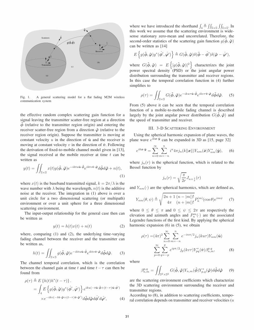
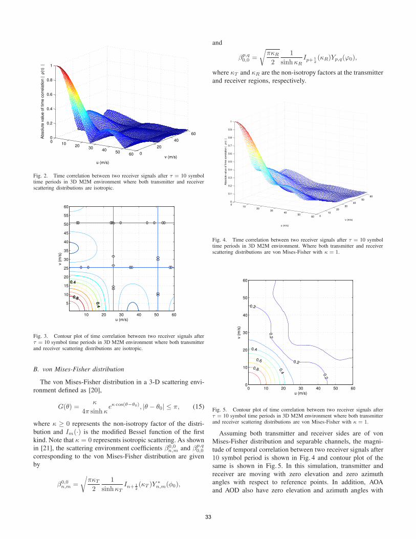
The magnitude of the time correlation between two receivedsignals after 10 symbol period versus magnitude of transmittervelocity and magnitude of receiver velocity are shown in Fig. 2and contour plot of the same is shown in Fig. 3, where bothtransmitter and receiver scattering distributions are isotropic.In this simulation, transmitter and receiver are moving withzero elevation and zero azimuth angles with respect to ref-erence points.The simulation result shows a high degree ofcorrelation (> 0.3) until both transmitter and receiver reach 20m/s and reduce to zero temporal correlation when transmitterand or receiver are at 25 m/s.

32

010

2030

4050

60 0

20

40

600

0.2

0.4

0.6

0.8

1

v (m/s)

u (m/s)

Abso

lute

valu

e o

f tim

e c

orr

ela

tion |

ρ(τ

) |

Fig. 2. Time correlation between two receiver signals after τ = 10 symboltime periods in 3D M2M environment where both transmitter and receiverscattering distributions are isotropic.

00

0

0

0

000

0

0

0

0

0.4

0.4

0.8

u (m/s)

v (m

/s)

00

0

0

0

000

0

0

0

0

0.4

0.4

0.8

10 20 30 40 50 60

5

10

15

20

25

30

35

40

45

50

55

60

Fig. 3. Contour plot of time correlation between two receiver signals afterτ = 10 symbol time periods in 3D M2M environment where both transmitterand receiver scattering distributions are isotropic.

B. von Mises-Fisher distribution

The von Mises-Fisher distribution in a 3-D scattering envi-ronment defined as [20],

G(θ) =κ

4π sinhκeκ cos(θ−θ0), |θ − θ0| ≤ π, (15)

where κ ≥ 0 represents the non-isotropy factor of the distri-bution and Im(·) is the modified Bessel function of the firstkind. Note that κ = 0 represents isotropic scattering. As shownin [21], the scattering environment coefficients β0,0

n,m and βp,q0,0

corresponding to the von Mises-Fisher distribution are givenby

β0,0n,m =

√

πκT

2

1

sinhκTIn+ 1

2

(κT )Y ∗n,m(φ0),

and

βp,q0,0 =

√

πκR

2

1

sinhκRIp+ 1

2

(κR)Yp,q(ϕ0),

where κT and κR are the non-isotropy factors at the transmitterand receiver regions, respectively.

010

2030

4050

60 0

10

20

30

40

50

60

0

0.1

0.2

0.3

0.4

0.5

0.6

0.7

0.8

0.9

1

v (m/s)

u (m/s)A

bso

lute

valu

e o

f tim

e c

orr

ela

tion |

ρ(τ

) |

Fig. 4. Time correlation between two receiver signals after τ = 10 symboltime periods in 3D M2M environment. Where both transmitter and receiverscattering distributions are von Mises-Fisher with κ = 1.

0.2

0.2

0.2

0.2

0.4

0.4

0.6

0.8

u (m/s)

v (m

/s)

0 10 20 30 40 50 600

10

20

30

40

50

60

Fig. 5. Contour plot of time correlation between two receiver signals afterτ = 10 symbol time periods in 3D M2M environment where both transmitterand receiver scattering distributions are von Mises-Fisher with κ = 1.

Assuming both transmitter and receiver sides are of vonMises-Fisher distribution and separable channels, the magni-tude of temporal correlation between two receiver signals after10 symbol period is shown in Fig. 4 and contour plot of thesame is shown in Fig. 5. In this simulation, transmitter andreceiver are moving with zero elevation and zero azimuthangles with respect to reference points. In addition, AOAand AOD also have zero elevation and azimuth angles with

33

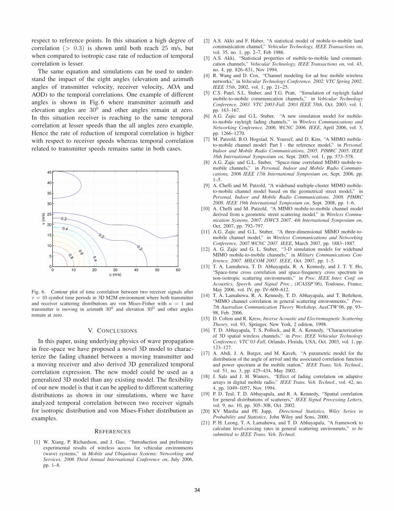
respect to reference points. In this situation a high degree ofcorrelation (> 0.3) is shown until both reach 25 m/s, butwhen compared to isotropic case rate of reduction of temporalcorrelation is lesser.

The same equation and simulations can be used to under-stand the impact of the eight angles (elevation and azimuthangles of transmitter velocity, receiver velocity, AOA andAOD) to the temporal correlations. One example of differentangles is shown in Fig. 6 where transmitter azimuth andelevation angles are 300 and other angles remain at zero.In this situation receiver is reaching to the same temporalcorrelation at lesser speeds than the all angles zero example.Hence the rate of reduction of temporal correlation is higherwith respect to receiver speeds whereas temporal correlationrelated to transmitter speeds remains same in both cases.

0.2

0.2

0.2

0.4

0.4

0.60.8

u (m/s)

v (m

/s)

0 10 20 30 40 50 600

5

10

15

20

25

30

35

40

45

Fig. 6. Contour plot of time correlation between two receiver signals afterτ = 10 symbol time periods in 3D M2M environment where both transmitterand receiver scattering distributions are von Mises-Fisher with κ = 1 andtransmitter is moving in azimuth 300 and elevation 300 and other anglesremain at zero.

V. CONCLUSIONS

In this paper, using underlying physics of wave propagationin free-space we have proposed a novel 3D model to charac-terize the fading channel between a moving transmitter anda moving receiver and also derived 3D generalized temporalcorrelation expression. The new model could be used as ageneralized 3D model than any existing model. The flexibilityof our new model is that it can be applied to different scatteringdistributions as shown in our simulations, where we haveanalyzed temporal correlation between two receiver signalsfor isotropic distribution and von Mises-Fisher distribution asexamples.

REFERENCES

[1] W. Xiang, P. Richardson, and J. Guo, “Introduction and preliminaryexperimental results of wireless access for vehicular environments(wave) systems,” in Mobile and Ubiquitous Systems: Networking andServices, 2006 Third Annual International Conference on, July 2006,pp. 1–8.

[2] A.S. Akki and F. Haber, “A statistical model of mobile-to-mobile landcommunication channel,” Vehicular Technology, IEEE Transactions on,vol. 35, no. 1, pp. 2–7, Feb 1986.

[3] A.S. Akki, “Statistical properties of mobile-to-mobile land communi-cation channels,” Vehicular Technology, IEEE Transactions on, vol. 43,no. 4, pp. 826–831, Nov 1994.

[4] R. Wang and D. Cox, “Channel modeling for ad hoc mobile wirelessnetworks,” in Vehicular Technology Conference, 2002. VTC Spring 2002.IEEE 55th, 2002, vol. 1, pp. 21–25.

[5] C.S. Patel, S.L. Stuber, and T.G. Pratt, “Simulation of rayleigh fadedmobile-to-mobile communication channels,” in Vehicular TechnologyConference, 2003. VTC 2003-Fall. 2003 IEEE 58th, Oct. 2003, vol. 1,pp. 163–167.

[6] A.G. Zajic and G.L. Stuber, “A new simulation model for mobile-to-mobile rayleigh fading channels,” in Wireless Communications andNetworking Conference, 2006. WCNC 2006. IEEE, April 2006, vol. 3,pp. 1266–1270.

[7] M. Patzold, B.O. Hogstad, N. Youssef, and D. Kim, “A MIMO mobile-to-mobile channel model: Part I - the reference model,” in Personal,Indoor and Mobile Radio Communications, 2005. PIMRC 2005. IEEE16th International Symposium on, Sept. 2005, vol. 1, pp. 573–578.

[8] A.G. Zajic and G.L. Stuber, “Space-time correlated MIMO mobile-to-mobile channels,” in Personal, Indoor and Mobile Radio Communi-cations, 2006 IEEE 17th International Symposium on, Sept. 2006, pp.1–5.

[9] A. Chelli and M. Patzold, “A wideband multiple-cluster MIMO mobile-to-mobile channel model based on the geometrical street model,” inPersonal, Indoor and Mobile Radio Communications, 2008. PIMRC2008. IEEE 19th International Symposium on, Sept. 2008, pp. 1–6.

[10] A. Chelli and M. Patzold, “A MIMO mobile-to-mobile channel modelderived from a geometric street scattering model,” in Wireless Commu-nication Systems, 2007. ISWCS 2007. 4th International Symposium on,Oct. 2007, pp. 792–797.

[11] A.G. Zajic and G.L. Stuber, “A three-dimensional MIMO mobile-to-mobile channel model,” in Wireless Communications and NetworkingConference, 2007.WCNC 2007. IEEE, March 2007, pp. 1883–1887.

[12] A. G. Zajic and G. L. Stuber, “3-D simulation models for widebandMIMO mobile-to-mobile channels,” in Military Communications Con-ference, 2007. MILCOM 2007. IEEE, Oct. 2007, pp. 1–5.

[13] T. A. Lamahewa, T. D. Abhayapala, R. A. Kennedy, and J. T. Y. Ho,“Space-time cross correlation and space-frequency cross spectrum innon-isotropic scattering environments,” in Proc. IEEE Inter. Conf. onAcoustics, Speech, and Signal Proc., (ICASSP’06), Toulouse, France,May 2006, vol. IV, pp. IV–609–612.

[14] T. A. Lamahewa, R. A. Kennedy, T. D. Abhayapala, and T. Betlehem,“MIMO channel correlation in general scattering environments,” Proc.7th Australian Communication Theory Workshop, AusCTW’06, pp. 93–98, Feb. 2006.

[15] D. Colton and R. Kress, Inverse Acoustic and Electromagnetic ScatteringTheory, vol. 93, Springer, New York, 2 edition, 1998.

[16] T. D. Abhayapala, T. S. Pollock, and R. A. Kennedy, “Characterizationof 3D spatial wireless channels,” in Proc. IEEE Vehicular TechnologyConference, VTC’03-Fall, Orlando, Florida, USA, Oct. 2003, vol. 1, pp.123–127.

[17] A. Abdi, J. A. Barger, and M. Kaveh, “A parametric model for thedistribution of the angle of arrival and the associated correlation functionand power spectrum at the mobile station,” IEEE Trans. Veh. Technol.,vol. 51, no. 3, pp. 425–434, May 2002.

[18] J. Salz and J. H. Winters, “Effect of fading correlation on adaptivearrays in digital mobile radio,” IEEE Trans. Veh. Technol., vol. 42, no.4, pp. 1049–1057, Nov. 1994.

[19] P. D. Teal, T. D. Abhayapala, and R. A. Kennedy, “Spatial correlationfor general distributions of scatterers,” IEEE Signal Processing Letters,vol. 9, no. 10, pp. 305–308, Oct. 2002.

[20] KV Mardia and PE Jupp, Directional Statistics, Wiley Series inProbability and Statistics, John Wiley and Sons, 2000.

[21] P. H. Leong, T. A. Lamahewa, and T. D. Abhayapala, “A framework tocalculate level-crossing rates in general scattering environmets,” to besubmitted to IEEE Trans. Veh. Technol.

34