3D Konstituvne Relacije Za Kost

Biomech Model Mechanobiol (2009) 8:149–165DOI 10.1007/s10237-008-0125-2

ORIGINAL PAPER

A three-dimensional elastic plastic damage constitutive lawfor bone tissue

David Garcia · Philippe K. Zysset ·Mathieu Charlebois · Alain Curnier

Received: 11 July 2007 / Accepted: 18 March 2008 / Published online: 9 April 2008© Springer-Verlag 2008

Abstract Motivated by mechanical analysis of bones andbone-implant systems, a 3D constitutive law describing themacroscopic mechanical behaviour of both cortical and tra-becular bone in cyclic (not fatigue) overloads is developed.The proposed model which mathematical formulation isestablished within the framework of generalized standardmaterials accounts for three distinct material evolution modeswhere elastic, plastic and damage aspects are closely related.The anisotropic elasticity of bone is described by a mor-phology-based model and distinct damage behaviour in ten-sion and compression by a halfspacewise generalized Hillcriterion. The plastic criterion is based on the intact elas-tic compliance tensor. The algorithm applies three distinctprojections based on the relationship between the internalvariables and criteria. Their respective consistent tangentoperators are presented. Numerical resolutions of severalboundary value problems and a biomechanical applicationare presented to illustrate the potential of the constitutivemodel and demonstrate the expected quadratic convergenceof the algorithm.

Keywords Bone tissue · Constitutive law · Damage ·Elasticity · Fabric · Plasticity

D. Garcia · A. CurnierLaboratory of Applied Mechanics and Reliability Analysis,Ecole Polytechnique Fédérale de Lausanne (EPFL),1015 Lausanne, Switzerland

P. K. Zysset (B) · M. CharleboisInstitute of Lightweight Design and Structural Biomechanics,Vienna University of Technology (TU-Wien),Gußhausstraße 27-29, 1040 Wien, Austriae-mail: [email protected]

1 Introduction

Bone tissue is traditionally subdivided into two types: cortical(compact) bone and trabecular (porous) bone, although theinterface between the two is somewhat fuzzy. This distinc-tion comes from its macroscopic appearance. At this level,the outer shell of a bone which is made of cortical bone can beclearly discerned from the inner core of the bone made of tra-becular bone. These two types of bone are identified by theirporosity, anisotropy and exhibit distinct material properties.

From a macroscopic mechanical point of view, both tissuesshow the same damage behaviour (i.e. progressive degrada-tion of their elastic properties Fondrk et al. 1999a; Keavenyet al. 1999) unless for excessive loads where trabecular bonecollapse occurs (not included in this study). A very similarmechanical behaviour is also observed between human andbovine bone tissue e.g. (Currey 2002; Fondrk et al. 1999a)suggesting that damage occurs at the ultrastructural level.Indeed, even if human and bovine bone differ at some hier-archical level of their structure e.g. Ascenzi et al. (1978), ifcortical and trabecular bone show different material proper-ties e.g. Cowin (2001); Fondrk et al. (1988), they share a sim-ilar ultrastructural organization (Rho et al. 1998) and showa qualitatively similar mechanical behaviour. Therefore, theobjective of this study is to formulate a single constitutivelaw which can be used for both types of bone.

Recently, new one-dimensional constitutive models forcortical bone tissue that straightforwardly predict the exper-imental damage stress–strain curve in cyclic uniaxial ten-sile and compressive loading at physiological strain rateswere proposed (Garcia 2006). As previous damage models(Fondrk et al. 1999b; Zysset 1994) did not succeed in describ-ing the reloading phase properly and/or did not include com-pressive loading, we chose to generalize to 3D the simplestrate-independent model presented in (Garcia 2006). The

123

150 D. Garcia et al.

approach chosen in this work is that of a macroscopic andphenomenological description of the mechanical behaviourof bone tissue. It accounts for three distinct evolution modesof deformation depending on two distinct criteria: an intactelastic regime, a simultaneous flow of rate-independentplasticity and damage and a rate-independent plasticitymode.

For a model to be applicable to both cortical and trabecularbone, it must be formulated in order to include the relevantarchitectural variables that can differentiate them i.e. vol-ume fraction (or structural density ρs defined by BV/TV i.e.bone volume/total volume) and fabric tensors that character-ize heterogeneity and anisotropy, respectively. Concerningthe elastic response of bone tissue, volume fraction (porous)and fabric-based elasticity models e.g. (Zysset and Curnier1995) have shown their validity (Zysset 2003) and were usedin our model. For the damaging behaviour of bone tissue, weopted for an alternative fabric-based damage criterion thatinvolves a reduced number of material constants (Zysset andRincón 2006) i.e. a halfspacewise generalization of the Hillcriterion that accounts for the distinct damage thresholds intension and compression of bone tissue. For simplicity, dam-age was defined as a scalar variable that affects equally allconstants of the elastic stiffness tensor which limits the appli-cability of the model to proportional loading and unloading.Furthermore, we restricted ourselves to the simplest aniso-tropic model for plasticity by choosing the fabric-based elas-tic compliance tensor to define the plastic yield criterion instress space e.g. Zysset and Curnier (1996).

The paper is organized as follows. Firstly, the constitu-tive model is formulated within the framework of general-ized standard materials in Sect. 2. Secondly, its algorithmicimplementation that involves consistent (algorithmic) tan-gent operators is presented in Sect. 3. Thirdly, the program-ming of the algorithm in a finite element code is validated inSect. 4 through a series of boundary value problems. Finally,the potential of the new 3D constitutive law is demonstratedby means of a mechanical analysis of the compression of avertebra in Sect. 5.

2 Constitutive model

2.1 Rheological setup and variables definition

The rheological model aims at describing the observedmacroscopic mechanical behaviour of bone tissue in cyclicoverloading situations. Interestingly, both cortical and tra-becular bone exhibit a similar mechanical behaviour sug-gesting that damage mechanisms occur at the ultrastructurallevel (Kotha and Guzelsu 2003; Keaveny et al. 2001, 1999;Fondrk et al. 1999a,b). Upon analyzing these experimentalresults, we retained three crucial regimes of deformation of

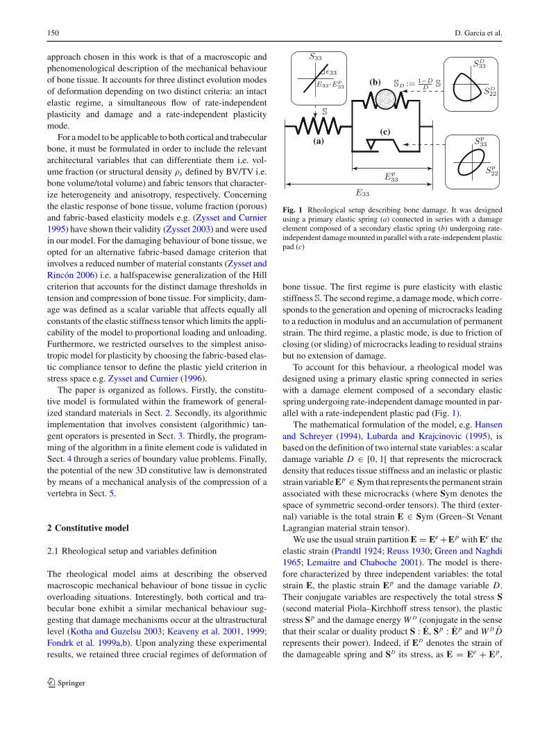
(a)

(b)

(c)

Fig. 1 Rheological setup describing bone damage. It was designedusing a primary elastic spring (a) connected in series with a damageelement composed of a secondary elastic spring (b) undergoing rate-independent damage mounted in parallel with a rate-independent plasticpad (c)

bone tissue. The first regime is pure elasticity with elasticstiffness S. The second regime, a damage mode, which corre-sponds to the generation and opening of microcracks leadingto a reduction in modulus and an accumulation of permanentstrain. The third regime, a plastic mode, is due to friction ofclosing (or sliding) of microcracks leading to residual strainsbut no extension of damage.

To account for this behaviour, a rheological model wasdesigned using a primary elastic spring connected in serieswith a damage element composed of a secondary elasticspring undergoing rate-independent damage mounted in par-allel with a rate-independent plastic pad (Fig. 1).

The mathematical formulation of the model, e.g. Hansenand Schreyer (1994), Lubarda and Krajcinovic (1995), isbased on the definition of two internal state variables: a scalardamage variable D ∈ [0, 1[ that represents the microcrackdensity that reduces tissue stiffness and an inelastic or plasticstrain variable Ep ∈ Sym that represents the permanent strainassociated with these microcracks (where Sym denotes thespace of symmetric second-order tensors). The third (exter-nal) variable is the total strain E ∈ Sym (Green–St VenantLagrangian material strain tensor).

We use the usual strain partition E = Ee +Ep with Ee theelastic strain (Prandtl 1924; Reuss 1930; Green and Naghdi1965; Lemaitre and Chaboche 2001). The model is there-fore characterized by three independent variables: the totalstrain E, the plastic strain Ep and the damage variable D.Their conjugate variables are respectively the total stress S(second material Piola–Kirchhoff stress tensor), the plasticstress Sp and the damage energy W D (conjugate in the sensethat their scalar or duality product S : E, Sp : Ep and W D Drepresents their power). Indeed, if ED denotes the strain ofthe damageable spring and SD its stress, as E = Ee + Ep,

123

Elastic plastic damage constitutive law for bone tissue 151

Ep = ED and S = Sp + SD , we have:

S : E = S : (Ee + Ep) = S : Ee + Sp : Ep + SD : ED. (1)

Three distinct evolutions in E, Ep, D space result formthe above described three regimes. In order to clarify the pre-sentation, we present now separately the properties of eachrheological element composing the model.

The primary linear spring with constant stiffness S (a pos-itive definite fourth-order tensor) mounted in series accountsfor the unaltered elastic response of the calcified extracellularbone matrix.

The plastic pad accounts for permanent strains due tomicrocracks. It is characterized by a plastic yield criterionwhich delimits a convex elastic domain in plastic stress space.If Sp denotes the stress in the plastic pad, let us define theelastic domain by:

Y p(Sp, D) ≤ 0 (2)

where Y p is the plastic yield function (to be defined) whichdepends on D to express the evolution of the domain withincreasing damage. The exact expression of Y p will be givenin Sect. 2.3 but let us mention that the initial radius of theelastic domain is chosen to be equal to 0 (i.e. Y p(Sp, 0) = 0)and that its hardening is isotropic.

The secondary linear (damageable) spring accounts forbone elastic damage due to microcracks. In analogy with theone-dimensional models presented by Garcia et al. (Garcia2006), the spring stiffness

SD := 1 − D

DS (3)

decreases from ∞ to 0 as the internal state variable D inc-reases from 0 to 1. As long as D is equal to zero, the stiffnessof the damageable spring is infinite due to the lack of ini-tial thickness of the crack and is thus equivalent to a rigidrod. Indeed, if the plastic pad is sliding, initially carrying nostress, the equivalent stiffness of the two springs mounted inseries becomes (1 − D) S which is the well-known result fora damaged elastic material. The damage variable D is there-fore limited between zero damage (D = 0) and full damage(D = 1) and has a simple interpretation e.g. (Lemaitre 1996).The assumption that damage affects equally all constants ofthe elastic stiffness tensor (isotropic damage) is not realisticeven for a linear elastic damageable material (e.g. He andCurnier 1995) but is reasonable for proportional loading.

Moreover, a damage threshold criterion which defines aconvex non-damaging domain is associated to the damage-able spring. If expressed in terms of the damage energy W D ,the non-damaging states are enclosed in the set

Y D(W D, D) ≤ 0 (4)

where Y D is the damage threshold function (to be defined)which also depends on D to express the evolution of thedomain with increasing damage. As many experiments onbone tissue have shown e.g. Cowin (2001), let us mentionthat the damage threshold criterion should include distincttensile and compressive threshold stresses (cf. Sect. 2.3).

2.2 Free energy and dissipation potentials

The nonlinear and rate-independent damage behaviour of themodel is entirely defined by two nonsmooth convex func-tions: a free energy potential that represents the stored elasticenergy density:

Ψ (E, Ep, D)

=

⎧⎪⎪⎨

⎪⎪⎩

12 (E − Ep) : S (E − Ep)

+ 12

1−DD Ep : S Ep + I[0,1[(D) if D > 0

12 E : S E + I{0}(Ep) if D = 0

(5)

and a dissipation potential that implicitly contains the evolu-tion rules for the internal variables:

Φ(Ep, D; E, Ep, D) := Φ p(Ep; D) + ΦD(D; E, Ep, D)

(6)

with

Φ p(Ep; D) := σ p(D)√

Ep : S Ep (7)

and

ΦD(D; E, Ep, D) := φ(D; E, Ep, D) + IR+(D) (8)

where

φ(D; E, Ep, D)

:={

h+(E, Ep, D)D if n(E, Ep) ≥ 0

h−(E, Ep, D)D if n(E, Ep) < 0. (9)

In Eqs. (5) and (8), I{.} is the indicator function of {.} definedas follows.

Let U be an arbitrary set and V a subset of U . We definethe indicator function of V as:

IV : U → {0,+∞}

x �→{

0 if x ∈ V+∞ if x /∈ V .

123


In Eq. (9), h± are the tensile/compressive damage energythresholds, respectively, defined by

h±(E, Ep, D)

:=

⎧⎪⎨

⎪⎩

r D2(D)

2(1 − D)2Ep : S Ep

S Ep : F±S Ep if ||Ep|| > 0

r D2(D)

2(1 − D)2E : S E

S E : F±S E if ||Ep|| = 0(10)

and n is the tension/compression criterion defined below.The functions σ p(D) and r D(D) that appear in Eqs. (7)

and (10) are the radii of the plastic and damage criteria,respectively. Their dependency with D expresses the increaseof stress during plastic flow and damage evolution. As men-tioned before, isotropic hardening will be considered in thiswork (cf. Sect. 2.3 for their explicit expression).

Distinct tensile and compressive threshold damagestresses are obtained with the halfspacewise generalizationof the Hill criterion proposed by Zysset and Rincón (2006).They appear in φ through the functions h± and the inter-face hyperplane n(E, Ep) = 0 dividing the strain space intotensile and compressive domains. The fourth-order tensorsF± define a non-symmetric non-damaging states set in dam-age stress space. The exact form of the criterion and of thehyperplane will be given in Sect. 2.3. In contrast with thevariables Ep and D, the arguments that appear in Φ afterthe semicolon symbol (;) (Eq. 6) are only parameters. Thedefinition (9) implies that the function φ, and thus Φ, is notcontinuous along Ep = 0. However, this discontinuity hasno incidence on the generalized standard material formalismbecause Ep is only a parameter (Ziegler 1983). The state lawswhich derive from the free energy potential are:

SΨ ∈ ∂ EΨ ={

S (E − Ep) if D ∈ ]0, 1[S E if D = 0

(11)

SpΨ ∈ −∂ EpΨ =

{S E − 1

D S Ep if D ∈ ]0, 1[Sym if D = 0

(12)

W DΨ ∈ −∂DΨ =

{1

2D2 Ep : S Ep if D ∈ ]0, 1[[0,∞[ if D = 0

(13)

where ∂ denotes the subdifferential e.g. Rockafellar (1970)and the ‘non-set’ quantities that appear in the right-hand sideof Eqs. (11)–(13) are to be considered as singletons. Thesame remark holds for further similar expressions.

To help the understanding of the model, let us define thestress in the damageable spring:

SD := SΨ − SpΨ ∈

{1−D

D S Ep if D ∈ ]0, 1[Sym if D = 0.

(14)

The complementary laws which derive from the dissipa-tion potential are:

SpΦ ∈ ∂ EpΦ

=

⎧⎪⎨

⎪⎩

σ p(D) S Ep√

Ep : S Epif ||Ep|| > 0

Sp | √Sp : E Sp − σ p(D) < 0 if ||Ep|| = 0

(15)

and

W DΦ ∈ ∂DΦ =

⎧⎪⎨

⎪⎩

φ′(E, Ep, D) if D >0

] − ∞, φ′(E, Ep, D)] if D =0

∅ if D <0

(16)

where E := S−1, φ′ is the derivative of φ with respect to

D, representing thus the tensile/compressive damage energythresholds h±, respectively, and ∅ is the empty set.

The dual dissipation potential is obtained via the Legen-dre–Fenchel transform:

Φ∗(Sp, W D; E, Ep, D)

:= supEp,D

[Sp : Ep + W D D − Φ(Ep, D; E, Ep, D)

].

As the dissipation potential is separate in Ep and D andas these variables are independent (uncoupled, mounted inparallel), the conjugate of the sum is simply the sum of theconjugates. Thus, we find:

Φ∗(Sp, W D; E, Ep, D)

= I[0,σ p(D)](√

Sp : E Sp) + I[−∞,φ′(E,Ep,D)](W D). (17)

The flow rules of the internal variables Ep and D are foundfrom the dual dissipation potential (inverse complementarylaws):

Ep ∈ ∂ SpΦ∗

=

⎧⎪⎪⎨

⎪⎪⎩

∅ if√

Sp : E Sp − σ p(D) > 0

Λp E Sp√Sp : ESp

if√

Sp : E Sp − σ p(D) = 0

0 if√

Sp : E Sp − σ p(D) < 0

(18)

with Λp ∈ [0,+∞[ a rate-like plastic Lagrangian multiplierand

D ∈ ∂ W D Φ∗

=

⎧⎪⎨

⎪⎩

0 if W D ∈ ] − ∞, φ′(E, Ep, D)[[0,+∞[ if W D = φ′(E, Ep, D)

∅ if W D > φ′(E, Ep, D)

. (19)

123


2.3 Elastic stiffness, plastic and damage criteria

Elastic stiffness

In order to reduce the number of elastic constants of ourmodel, we use the orthotropic morphology–based Zysset–Curnier model (Zysset and Curnier 1995; Zysset 1994) thatrelates the elastic properties of a porous material and its geo-metric symmetry.

The solid microstructure of an elastic porous solid likebone is characterized by the solid volume fraction ρs whereasits structural anisotropy by the second-order fabric tensor:

M := mi mi ⊗ mi (20)

where i = 1, 2, 3 and the normalization det (M) = 1 holds(Kanatani 1984; Cowin 1985). The eigenvectors mi (or prin-cipal directions) provide the normal directions of the ortho-tropic symmetry planes whereas the eigenvalues mi reflectthe extent of anisotropy. The tensors Mi = mi ⊗ mi arecalled the structural tensors.

In terms of the structural tensors, the compliance tensorE = S

−1 is given by:

E =3∑

i=1

1

εiMi ⊗ Mi −

3∑

i, j=1; i �= j

νi j

εiMi ⊗ M j

+3∑

i, j=1; i �= j

1

2µi jMi ⊗ M j (21)

where the orthotropic engineering constants are:

εi = ε0 ρks m2l

i , (22)

νi j = ν0ml

i

mlj

, (23)

µi j = µ0 ρks ml

i mlj (24)

and the double tensorial product of second-order tensors isdefined by (Curnier et al. 1995):

(A ⊗ B)X = 1

2AXBT ∀X = XT (25)

The constants ε0, ν0 and µ0 represent the extrapolated elasticconstants of the plain (poreless) isotropic material. Thus, theorthotropic elasticity of bone tissue is approximated by theconstants ε0, ν0 and µ0, the porosity exponent k, the anisot-ropy exponent l, the volume fraction ρs and the fabric tensorM. The good results obtained by Zysset (1994) for the elasticconstants of compact bone extrapolated from those of tra-becular bone show the relevance of using morphology-basedelasticity for bone tissue (see also Zysset 2003).

Plastic criterion

The relation (15) defines a convex elastic domain which ischaracterized by the plastic yield function Y p(Sp, D) alreadymentioned in (2) and now defined by:

Y p(Sp, D) := √Sp : E Sp − σ p(D). (26)

The function σ p(D) describes the radius of the plastic yieldcriterion and its evolution with increasing damage (isotropichardening). By analogy with the one-dimensional models ofGarcia (2006), let us define:

σ p(D) := χ p(1 − exp(−wD)) (27)

where χ p and w are two positive plastic hardening parame-ters, to be identified on experimental grounds.

In the Kuhn–Tucker form, the flow rule and the elasticdomain read:

Ep = Λp Np(Sp), Np(Sp) := ∂Y p

∂Sp (Sp),

Y p(Sp, D) ≤ 0, Λp ≥ 0, Λp Y p(Sp, D) = 0.(28)

The first line of equations is the associated flow rule whichdefines the plastic strain rate direction as an outward normal(not unitary) to the convex elastic domain in stress space.The second line of inequalities expresses the plastic yieldand consistency conditions. Note that we restricted ourselvesto the simplest anisotropic model for plasticity by choosingthe elastic compliance tensor E to define the convex elasticdomain (Zysset 1994). As mentioned before (Sect. 2.1), thechoice σ p(0) = 0 is made i.e. in the absence of damage, theplastic pad carries zero stress.

Damage criterion

Equation (16) leads us to define the damage threshold func-tion Y D that delimits a non-damaging convex domain. For||Ep|| > 0 and D �= 0, it reads:

Y D(W D; E, Ep, D)

:=

⎧⎪⎪⎪⎪⎪⎪⎨

⎪⎪⎪⎪⎪⎪⎩

√

2(1 − D)2W D S Ep : F+S Ep

Ep : S Ep

−r D(D) ≤ 0 if n(E, Ep) ≥ 0√

2(1 − D)2W D S Ep : F−S Ep

Ep : S Ep

−r D(D) ≤ 0 if n(E, Ep) < 0

(29)

123


and for ||Ep|| = 0 and D �= 0:

Y D(W D; E, 0, D)

:=

⎧⎪⎪⎪⎪⎪⎨

⎪⎪⎪⎪⎪⎩

√

2(1 − D)2W D S E: F+S EE: S E

−r D(D) ≤ 0 if n(E, 0) ≥ 0√

2(1 − D)2W D S E: F−S EE: S E

−r D(D) ≤ 0 if n(E, 0) < 0

(30)

which is strictly equivalent to the following halfspacewisegeneralized Hill criterion (Hill 1950):

Y D(SD; D)

:={√

SD : F+ SD − r D(D) ≤ 0 if m(SD) ≥ 0√

SD : F− SD − r D(D) ≤ 0 if m(SD) < 0(31)

where m(SD) is the stress interface plane defined below.The damage criterion (29) for ||Ep|| > 0 and D �= 0

is non-smoothly connected to the damage criterion (30) for||Ep|| = 0 and D �= 0 because of the non-continuous defi-nition of the damage dissipation potential along Ep = 0, cf.Eq. (8). However, the parallel mounting of the plastic pad andof the damage element associated to the definition of theirrespective criteria avoids any significant numerical problem.Indeed, for D �= 0, Ep vanishes only when the plastic pad issliding alone with no accumulation of damage (pure plasticmode, cf. Sect. 3.1).

For D = 0, W D and thus SD are undefined (cf. Eqs. (13)and (14)) and a global equivalent criterion must be definedas done in Sect. 3.1, Eq. (44).

The function n(E, Ep) already introduced in (9) is thefunction dividing the strain space into tensile and compres-sive domains. It can be shown (Curnier et al. 1995) that:

n(E, Ep) ={

N : Ep if ||Ep|| �= 0

N : E if ||Ep|| = 0(32)

where N is the unit normal tensor to the interface hyperplanen(E, Ep) = 0 which expression will be given below (Eq.40). Complementarily, the function m(SD) is the functiondividing the damage stress space into tensile and compres-sive domains. It reads (Curnier et al. 1995):

m(SD) = N : SD (33)

where N is the unit normal tensor to the interface hyperplanem(SD) = 0.

In terms of volume fraction and the fabric tensor, the gen-eral forms of the fourth-order tensors F± are (Zysset andRincón 2006):

F+ =3∑

i=1

1

(σ+i i )2

Mi ⊗ Mi −3∑

i, j=1; i �= j

χ+i j

(σ+i i )2

Mi ⊗ M j

+3∑

i, j=1; i �= j

1

2τ 2i j

Mi⊗M j (34)

F− =3∑

i=1

1

σ−i i

2 Mi ⊗ Mi −3∑

i, j=1; i �= j

χ−i j

(σ−i i )2

Mi ⊗ M j

+3∑

i, j=1; i �= j

1

2τ 2i j

Mi⊗M j (35)

σ+i i (ρs, m1, m2, m3) and σ−

i i (ρs, m1, m2, m3) are the uniax-ial tensile and compressive strengths along the axis of indexi = 1, 2, 3, τi j (ρs, m1, m2, m3) are the shear strengths in theplane of index i, j = 1, 2, 3; i �= j , χ+

i j (ρs, m1, m2, m3)

and χ−i j (ρs, m1, m2, m3) are stress interaction coefficients.

Following the approach used in fabric elasticity (Zysset andCurnier 1995), power functions are selected for the depen-dence of the material properties with volume fraction andfabric eigenvalues:

σ+i i = σ+

0 ρp

s m2qi , σ−

i i = σ−0 ρ

ps m2q

i , τi j = τ0ρp

s mqi mq

j ,

χ+i j = χ+

0

m2qi

m2qj

, χ−i j = χ−

0

m2qi

m2qj

, (36)

where σ+0 and σ−

0 are the uniaxial tensile and compressivestrengths, τ0 is the shear strength, χ+

0 and χ−0 are interaction

coefficients for a poreless (ρs = 1) bone material with atleast cubic symmetry (m1 = m2 = m3 = 1). These valuescan be obtained by multiple linear regression of experimen-tal anisotropic strength data of bone tissue, e.g. Zysset andRincón (2006). The exponent p is associated with porosityand q is associated with anisotropy of the fabric-based dam-age criterion Y D .

Continuity and differentiability of the damage criterionY D leads to:

χ−0 + 1

(σ−0 )2

= χ+0 + 1

(σ+0 )2

(37)

and to an expression for the normal hyperplane tensor (Zyssetand Rincón 2006):

N = αi Mi (38)

where Mi are the structural tensors and αi the interface hyper-plane coefficients given by:

αi =

√√√√√

1m4q

i∑3

i=11

m4qi

. (39)

123


Fig. 2 Left: Shape of damagethreshold criterion in the spaceof normal damage stresses withrespect to the orthotropic planesof symmetry of bone tissue.Middle: Its intersection with theplane SD

11 = SD22 that contains

the axis of hydrostatic pressure.Right: Its intersection with theplane SD

33 = 0. The hyperplanem(SD) = 0 which orientationdepends on the fabriceigenvalues divides the damagestress space into tensile andcompressive domains

The normal tensor in strain space is given by (Curnier et al.1995):

N = F−1+ N = F

−1− N. (40)

Finally, let us define the radius of the damage criterionr D(D). It evolves with increasing damage according to (iso-tropic hardening):

r D(D) := R(1 + χ D (1 − exp(−vD))

)(41)

where χ D and v are two damage hardening parameters. Theconstant R is an additional (redundant) parameter whichcould be omitted and incorporated in the definition of F±. Itcorresponds to the initial radius of the damage criterion.

In summary, given volume fraction and fabric values, a setof six material constants define the non-symmetric damagecriterion (plus two for the isotropic hardening function). Theshape of the halfspacewise damage criterion is illustrated inFig. 2.

3 Numerical algorithm

In order to implement the model in a finite element mechani-cal analysis software, the elastic plastic damage evolution lawneeds to be discretized in time. Its algorithmic implementa-tion is presented in detail in the following as it applies threenon-trivial projections based on the relationship between thetwo internal variables and their corresponding criteria.

3.1 Time integration algorithm with projections

Assume that we have an initial strain state En , Epn , Dn to

start with for any given discretized time increment tn withinitial damage Dn �= 0. To this state corresponds the uniqueinitial stress state Sn , Sp

n , W Dn defined by the state laws (11),

(12) and (13). W Dn is the initial damage energy. This state is

supposed to be plastically and damageably admissible in thesense that it satisfies both plastic and damage criteria:

Y p(Spn , Dn) ≤ 0 and Y D(W D

n , En, Epn , Dn) ≤ 0. (42)

Given a new total strain En+1, integrating the flow ruleconsists of finding a new plastic strain Ep

n+1 and a new dam-age state variable Dn+1 such that the final state defined forthe time instant tn+1 by En+1, Ep

n+1, Dn+1 and correspond-ing final stress state Sn+1, Sp

n+1, W Dn+1 will also be plastically

and damageably admissible i.e.

Y p(Spn+1, Dn+1) ≤ 0 and

Y D(W Dn+1, En+1, Ep

n+1, Dn+1) ≤ 0. (43)

To this end, a trial strain state is first considered in theform En+1, Ep

n , Dn and corresponding trial stress state ST :=S(En+1, Ep

n ), SpT :=Sp(En+1, Ep

n , Dn), W DT :=W D(Ep

n , Dn)

which may be non-admissible. The final state is then reachedby projecting the trial state on the convex plastic and dam-age sets enclosed by the corresponding yield and thresholdsurfaces.

If Dn = 0, then SpT and W D

T are undefined (Eqs. (12) and(13)). Thus, the yield and damage criteria cannot be tested.The indetermination can be lifted by defining a global equiv-alent criterion which depends on the trial total stress:

Y (ST) :=⎧⎨

⎩

√ST : F+ ST − r D(0) if m(ST) ≥ 0

√ST : F− ST − r D(0) if m(ST) < 0

. (44)

In the case of damage process i.e.Y (ST) > 0, the final valuesof Sp

n+1 and W Dn+1 are well defined at the projection point

Y p(Spn+1, Dn+1)=0 and Y D(W D

n+1, En+1, Epn+1, Dn+1)=0

and normality of the flow rule is guaranteed through the incre-mental process.

In the following, we assume that Dn �= 0 and present thethree distinct projections for the three modes of evolution ofthe model.

123


a) Elastic mode: Y p(SpT , Dn) ≤ 0 and Y D(W D

T , En+1, Epn ,

Dn) ≤ 0

In this case, we simply have Epn+1 = Ep

n and Dn+1 = Dn .

b) Pure plastic mode: Y p(SpT , Dn) > 0 and Y D(W D

T , En+1,

Epn , Dn) ≤ 0

In this case, we only must satisfy Y p(Spn+1, Dn+1) = 0. The

relation between the initial and new plastic strains is givenby the incremental flow rule for ∆Ep

n+1 :

∆Epn+1 = λp Np(Sp

n+1) (45)

where ∆Epn+1 is the plastic strain increment, λp is the plastic

Lagrangian multiplier and Np(Spn+1) is the outward normal

of the plastic criterion, cf. Eq. (28), evaluated at the finalunknown stress state Sp

n+1. Therefore, it is an implicit pro-jection algorithm (Simo and Hughes 1999).

Combining Epn+1 = Ep

n + ∆Epn+1 and Dn+1 = Dn and

solving for Spn+1, we get the analytical expression for the

plastic multiplier (Curnier 1993):

λp = Dn Y p(SpT , Dn). (46)

As the final plastic stress is collinear to the trial stress, theprojection is radial (Wilkins 1964; Moreau 1979).

c) Damage and plastic mode: Y p(SpT , Dn) > 0 and Y D

(W DT , En+1, Ep

n , Dn) > 0

In this case, we must satisfy simultaneously:

{Y p(Sp

n+1, Dn+1) = 0 and

Y D(W Dn+1, En+1, Ep

n+1, Dn+1) = 0.

The final plastic strain is again computed via the incrementalflow rule for ∆Ep

n+1 i.e. Epn+1 = Ep

n + ∆Epn+1 with ∆Ep

n+1given by Eq. (45). This time, the final damage must be deter-mined and is given by the rule Dn+1 = Dn + ∆Dn+1 where∆Dn+1 is the damage increment.

By computing the final plastic stress and injecting itsexpression in the plastic criterion, the following plastic mul-tiplier is found (Garcia 2006):

λp =√

(Dn+1En+1 − Epn ) : S (Dn+1En+1 − Ep

n )

−Dn+1 σ p(Dn+1). (47)

The final damage state variable Dn+1 remains to be found.To this end, we use the projection of W D

T (or equivalently ofSD

T ) on the damage criterion.By computing the final damage stress SD

n+1 as a functionof En+1, Ep

n and Dn+1, let us define the damage solutionfunction f± : [0, 1[ → R by:

f±(Dn+1) := SDn+1 : F± SD

n+1 − r D2(Dn+1)

=(

1 − Dn+1

λp + Dn+1 σ p(Dn+1)

)2

×(λp2

S En+1 : F±S En+1++ 2λpσ p(Dn+1) S En+1 : F±S Ep

n ++ σ p2(Dn+1) S Ep

n : F±S Epn

)− r D2(Dn+1)

(48)

with F+ for m(SDT ) > 0 and F− for m(SD

T ) < 0, respectively,and λp = λp(Dn+1) given by (47). As En+1 is assumed tobe known (or predicted), the value of Dn+1 can be found bysolving f±(Dn+1) = 0.

We use the generalized Newton method (Alart and Curnier1991) in order to solve this nonsmooth C0 nonlinear equationi.e. if D j

n+1 is the damage variable at iteration j :

D j+1n+1 = D j

n+1 − f±(D jn+1)

f±′(D jn+1)

with

j = 0, 1, 2, . . . and D0n+1 = Dn (49)

where f±′ is the derivative of f± with respect to Dn+1. Onlyonce the final damage variable Dn+1 has been found, theplastic multiplier λp defined in Eq. (47) has to be updated.

3.2 Incremental linearization algorithm

For a uniform deformation test with a homogeneous stressstate, a situation occurring in a single finite element, the prob-lem is equivalent to the following local problem: find En+1

such that the equation of force equilibrium is satisfied i.e.:

S(En+1, Epn+1, Dn+1) − S = 0

where S denotes the imposed stress. We also use the gener-alized Newton method to solve this problem i.e. if Ei is thestrain tensor at iteration i :

Ei+1n+1 = Ei

n+1 + ∆Ein+1 with i = 0, 1, 2, . . . (50)

where

∆Ein+1 = −P

−1(Ein+1, Ep

n+1, Dn+1)

×(

S(Ein+1, Ep

n+1, Dn+1) − S)

(51)

is the total strain increment at iteration i and P := dSdE is the

total stress derivative with respect to the strain. That meansthat the determination of En+1 requires the computation ofthe tangent operator P. Two different tangent operators canbe defined depending on the type of flow and evolution ruleswhich are linearized. The linearization of the continuum rules

123


leads to the continuous tangent operator whereas the line-arization of the incremental rules leads to the algorithmic(consistent) tangent operator. In order to simplify the nota-tions of the continuous and incremental tangent operators,we omitted the subscripts n+1 wherever they have to be usedi.e. for the internal variables and the different stresses. Theiranalytic expressions are presented in the following two sub-sections, cf. Garcia (2006) for a detailed description of theircomputation.

3.3 Continuous tangent operators

We present now the continuous tangent operator P := dSdE

required by the Newton method (50) for the three evolutionmodes of the model (Pe for the elastic, P

p for the plastic andP

D for the damage mode, respectively). The word continuousrefers to a velocity-based definition of the tangent operator,opposed to an incremental definition.

a) Elastic mode: case Ep = 0 and D = 0

In this case, we simply have:

Pe = S. (52)

b) Plastic mode: case Ep �= 0 and D = 0

The plastic stiffness tensor reads:

Pp = S − D

S Np(Sp) ⊗ S Np(Sp)

Np(Sp) : S Np(Sp). (53)

It is a rank-1 modification of the elasticity tensor as usual,but this modification is scaled by the damage intensity D.

c) Damage mode: case Ep �= 0 and D > 0

The expression of the damage continuous tangent operatoris:

PD =S − D

[Np(Sp) : S Np(Sp)

+(1 − D)D2 ∂Y p

∂ D + Np(Sp) : S Ep

D2 ∂Y D

∂ D − ND(SD) : S Ep·

·ND(SD) : S Np(Sp)]−1

S Np(Sp) ⊗ S Np(Sp) (54)

with ND(SD) := ∂Y D

∂SD the outward normal of the damage

criterion in stress space. The damage stiffness tensor is againa scaled rank-1 modification of the elasticity tensor, but thescaling factor is more complicated due to the hardening rulesof both plastic and damage criteria. The damage continuumtangent operator is symmetric.

3.4 Incremental tangent operators

For any discretized computer implementation of the consti-tutive law, the total strain increment does not tend to zero.Therefore, the incremental or algorithmic form Pa of the con-tinuous tangent operator P has to be determined (Simo andTaylor 1985).

Once again, we proceed in three steps and only present thefinal results (Pe

a for the elastic, Ppa for the plastic and P

Da for

the damage algorithmic tangent operator, respectively). Theinterested reader will find a concise derivation of P

pa and P

Da

in the appendix. We remind that all internal variables and thedifferent stresses appearing in the following expressions areto be evaluated at the final (pseudo) time instant tn+1.

a) Elastic mode: case ∆Ep = 0 and ∆D = 0

As in the continuous case, we have:

Pea = S. (55)

b) Plastic mode: case ∆Ep �= 0 and ∆D = 0

In that mode, we find:

Ppa = (1 − D) S + D

[

Sa − Sa Np(Sp) ⊗ Sa Np(Sp)

Np(Sp) : Sa Np(Sp)

]

(56)

where Sa :=[E + λp

D Hp(Sp)

]−1and H

p(Sp) := ∂2Y p

∂Sp2 .

If λp = 0, then Sa = S and Ppa = P

p, which is consis-tent with the continuous description. In the absence of thedamageable spring, dS = dSp. Thus

Pa = Sa − Sa Np(Sp) ⊗ Sa Np(Sp)

Np(Sp) : Sa Np(Sp)

which is the algorithmic tangent operator for perfect elasto-plasticity found by Rakotomanana et al. (1991).

c) Damage mode: case ∆Ep �= 0 and ∆D > 0

The damage incremental tangent operator has the form:

PDa =S [I−A]−1[ (I−A)−D (I−E Sad)− D

αE Sad (I−A) B ]

(57)

with I the symmetric fourth-order identity tensor,

A := (1 − D) Ep ⊗ S ND(SD)

ND( SD) : S Ep − ∂Y D

∂ D D2, (58)

Sad :=[

E + λp

D(I − A) H

p(Sp)

]−1

, (59)

123


α := Np(Sp) : Sad (I − A)Np(Sp) − ∂Y p

∂ DD(1 − D) ·

· D ND(SD) : S Np(Sp)−λp ND(SD) : S Hp(Sp) Sad (I−A) Np(Sp)

ND(SD) : S Ep − ∂Y D

∂ D D2

(60)

and

B :=[

Np(Sp) ⊗ Sad Np(Sp)+

+∂Y p

∂ DD(1 − D)λp

× Np(Sp) ⊗ ND(SD)

ND(SD) : S Ep − ∂Y D

∂ D D2S H

p(Sp) Sad

]

.

(61)

If λp = 0, then Sad = S, B = Np(Sp) ⊗ S Np(Sp) and α =Np(Sp) : S Np(Sp)−(1−D)

Np( Sp): S Ep+ ∂Y p∂ D D2

ND( SD): S Ep− ∂Y D∂ D D2

ND(SD) :S Np(Sp), which is consistent with the continuous descrip-tion. In the absence of the damageable spring ND(SD) = 0,thus A vanishes and Sad = Sa . Thus P

Da = P

pa which is the

algorithmic tangent operator for perfect elasto-plasticity.

4 Validation

The validation was first achieved by testing a single finite ele-ment with appropriate one-dimensional schedules and thenboundary value problems were chosen in order to check theconvergence of the implicit projection algorithms. But firstof all, let us present the material constants used in our simu-lations.

4.1 Material constants

Volume fraction and fabric

The values are summarized in Table 1. We use the classi-cal mean value of 0.9 for cortical bone volume fraction thataccounts for residual porosity associated with the vascularHavers and Volkmann canals as well as the lacunae (Cowin2001). For simplicity, we choose a 1 to 10 ratio between tra-becular and cortical bone volume fraction which is somewhatarbitrary. The mean values found by Zysset (1994) are usedfor fabric, with the normalization det(M) = 1.

Table 1 Volume fraction and fabric values from Cowin (2001), Zysset(1994)

ρcorts ρtrab

s m1 m2 m3

0.9 0.09 0.894 0.894 1.252

Table 2 Fabric-based Zysset–Curnier elasticity model parameters fromZysset (1994)

ε0 (GPa) µ0 (GPa) ν0 k l

15.75 5.28 0.32 2.0 1.0

Table 3 Material constants of the fabric-based halfspacewise damagecriterion identified for trabecular bone in Zysset and Rincón (2006),Rincón (2003)

σ−0 (MPa) σ+

0 (MPa) τ0 (MPa) χ−0 χ+

0 p q

58.4 43.3 23.1 0.31 −0.28 1.32 0.56

Table 4 Identified hardening parameters, based on our own corticalbone uniaxial tests (Garcia 2006)

χ p (MPa1/2) w χ D v Rcort Rtrab

0.12 14 5.12 14 0.33 1.0

Morphology-elasticity

We use the porous elasticity described by volume fractionand the second-order fabric tensor (Zysset–Curnier model,Eq. 21). Table 2 summarizes the values of the constants ofthe plain isotropic bone together with the exponents k andl characterizing its volume fraction and anisotropy, respec-tively.

Halfspacewise damage criterion

As the damage criterion is also expressed in terms of volumefraction and fabric, the constants presented in Table 3 areused to define its shape in stress space for both cortical andtrabecular bone (cf. Eq. 31). Its initial radius R is specifiedfor both types of bone in Table 4.

Plastic and damage hardening parameters

Table 4 shows the values used for the plastic and damagehardening parameters (Eqs. (27) and (41)).

As some of these material constants are based on humanand other on bovine bone experiments, the latter valuesshould be identified in subsequent human studies. However,we expect to obtain satisfying qualitative results due to thesimilar composition of these tissues. Note that as both dissi-pative mechanisms (plastic and damage) are closely related(there is no damage evolution without plastic slip), a separateidentification of the corresponding parameters is a difficulttask. Indeed, the hardening function of plasticity influencesthe extent of the hysteresis during the purely plastic modewhile both plasticity and damage hardening functions con-tribute to the hardening curve during the combined damage

123


12

3

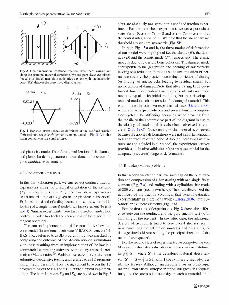
Fig. 3 One-dimensional confined traction experiment carried outalong the principal material direction (left) and pure shear experiment(right) of a single linear eight-node brick element with one integrationpoint. u(t) denotes the prescribed displacement

Strain Strain

Fig. 4 Imposed strain schedules definition of the confined traction(left) and pure shear (right) experiments presented in Fig. 3. All otherstrain components are equal to zero.

and plasticity mode. Therefore, identification of the damageand plastic hardening parameters was done in the sense of agood qualitative agreement.

4.2 One-dimensional tests

In this first validation part, we carried out confined tractionexperiments along the principal orientation of the material(E11 = E22 = 0, E33 = E33) and pure shear experiments(with material constants given in the previous subsection).Each test consisted of a displacement-based, saw-tooth likeloading of a single linear 8-node brick finite element (Figs. 3and 4). Similar experiments were then carried out under loadcontrol in order to check the correctness of the algorithmictangent operators.

The correct implementation of the constitutive law in acommercial finite element software (ABAQUS, version 6.4,HKS, Inc.), referred to as 3D programming, was checked bycomparing the outcome of the aforementioned simulationswith those resulting from an implementation of the law in acommercial computing software without any space discret-ization (Mathematica�, Wolfram Research, Inc.), the lattersubmitted to extensive testing and referred to as 1D program-ming. Figure 5 a and b show the agreement between the 1Dprogramming of the law and its 3D finite element implemen-tation. The lateral stresses S11 and S22 are not shown in Fig. 5

a but are obviously non-zero in this confined traction exper-iment. For the pure shear experiment, we get a pure shearstate S31 �= 0, S12 = S23 = 0 and S11 = S22 = S33 = 0 atthe central integration point. We note that the shear damagethreshold stresses are symmetric (Fig. 5b).

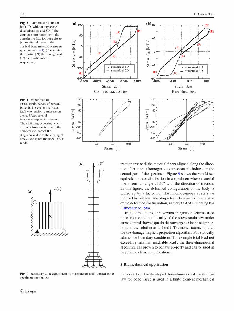
In both Figs. 5 a and b, the three modes of deformationof our model were highlighted i.e. the elastic (E), the dam-age (D) and the plastic mode (P), respectively. The elasticmode is due to reversible bone cohesion. The damage modecorresponds to the generation and opening of microcracksleading to a reduction in modulus and accumulation of per-manent strains. The plastic mode is due to friction of closing(or sliding) of microcracks leading to residual strains butno extension of damage. Note that after having been over-loaded, bone tissue unloads and then reloads with an elasticmodulus equal to its initial modulus, but then develops areduced modulus characteristic of a damaged material. Thisis confirmed by our own experimental tests (Garcia 2006)which shows respectively one and several tension–compres-sion cycles. The stiffening occurring when crossing fromthe tensile to the compressive part of the diagram is due tothe closing of cracks and has also been observed in con-crete (Ortiz 1985). No softening of the material is observedbecause the applied deformations were not important enoughto lead to fracture of the bone. Although these two last fea-tures are not included in our model, the experimental curvesprovide a qualitative validation of the proposed model for theadequate (moderate) range of deformation.

4.3 Boundary values problems

In this second validation part, we investigated the pure trac-tion and compression of a bar starting with one single finiteelement (Fig. 7 a) and ending with a cylindrical bar madeof 800 elements (not shown here). Then, we discretized thegeometry of the traction specimens that were investigatedexperimentally in a previous work (Garcia 2006) into 1848-node brick linear elements (Fig. 7 b).

For the first class of experiments, Fig. 8 shows the differ-ence between the confined and the pure traction test (withshrinking of the element). In the latter case, the additionaldegrees of freedom (related to zero lateral stresses) resultin a lower longitudinal elastic modulus and thus a higherdamage threshold stress along the principal direction of thematerial as expected.

For the second class of experiments, we computed the vonMises equivalent stress distribution in the specimen, defined

as√

32 ||S′|| where S′ is the deviatoric material stress ten-

sor (S′ := S − 13 Tr S I, with I the symmetric second-order

identity tensor). Although inappropriate for an orthotropicmaterial, von Mises isotropic criterion still gives an adequateimage of the stress state intensity in such a material. In a

123


Fig. 5 Numerical results forboth 1D (without any spacediscretization) and 3D (finiteelement) programming of theconstitutive law for bone tissue(simulation done with thecortical bone material constantsgiven in Sect. 4.1). (E) denotesthe elastic, (D) the damage and(P) the plastic mode,respectively

numerical 1Dnumerical 1Dnumerical 3Dnumerical 3D

(E)

(E)

(E)

(E)

(E)

(E)(P)

(P)

(P)(P)

(D)

(D)

(D)

Strain E33

Stre

ssS

33[M

Pa]

Strain E31

Stre

ssS

31[M

Pa]

Confined traction test Pure shear test

(a) (b)

Fig. 6 Experimentalstress–strain curves of corticalbone during cyclic overloads.Left: one tension–compressioncycle. Right: severaltension–compression cycles.The stiffening occurring whencrossing from the tensile to thecompressive part of thediagrams is due to the closing ofcracks and is not included in ourmodel

Stre

ss[M

Pa]

Strain [−]St

ress

[ MP

a]

Strain [−]

(a)

(b)

Fig. 7 Boundary value experiments: a pure traction and b cortical bonespecimen traction test

traction test with the material fibers aligned along the direc-tion of traction, a homogeneous stress state is induced in thecentral part of the specimen. Figure 9 shows the von Misesequivalent stress distribution in a specimen whose materialfibers form an angle of 30o with the direction of traction.In this figure, the deformed configuration of the body isscaled up by a factor 50. The inhomogeneous stress stateinduced by material anisotropy leads to a well-known shapeof the deformed configuration, namely that of a buckling bar(Timoshenko 1968).

In all simulations, the Newton integration scheme usedto overcome the nonlinearity of the stress-strain law understress control showed quadratic convergence in the neighbor-hood of the solution as it should. The same statement holdsfor the damage implicit projection algorithm. For staticallyadmissible boundary conditions (for example total load notexceeding maximal reachable load), the three-dimensionalalgorithm has proven to behave properly and can be used inlarge finite element applications.

5 Biomechanical application

In this section, the developed three-dimensional constitutivelaw for bone tissue is used in a finite element mechanical

123


Strain E33

Stre

ssS

33[M

Pa]

confined tractionpure traction

Fig. 8 Confined and pure traction tests carried out on a single finiteelement whose principal material direction is aligned along the directionof traction (for the same material constants as Fig. 5)

Fig. 9 Traction test carried out on cortical bone specimen with materialfibers forming an angle of 30o with the direction of traction (deforma-tion scale: ×50). The specimen twist is characteristic of orthotropy

analysis software (ABAQUS) in order to assess the mechan-ical state of a lumbar vertebra under uniaxial load by means oftwo plano-parallel polymethyl methacrylate (PMMA) plates.The vertebra is constituted of an external cortical bone shelland an internal trabecular bone core. As we consider trabecu-lar bone as porous cortical bone, mechanically speaking, thesame damage model is used for both bone tissues but withdifferent material constants. We are aware that the predic-tions concerning the internal state of the lumbar vertebra areonly illustrative and are intended to show the potential of thenovel three-dimensional law.

The mesh of the vertebral body was generated from highresolution quantitative computed tomography (Xtreme CT,

Scanco Medical, Switzerland). The mesh of the twosurrounding PMMA plates were extruded from the superiorand inferior endplate. Both cortical and trabecular bone ele-ments are 10-node quadratic tetrahedron elements (forming atotal of 65, 131 elements). Several simplifications were madeconcerning the material orientations of the bone elementsand their material constants. Firstly, the material symmetrywas assumed to be transverse isotropic with a uniform direc-tion of anisotropy following the direction of the mechani-cal solicitation (vertical). Secondly, the material constants ofboth cortical and trabecular bone elements (and particularlytheir densities) were assumed to be uniform. The materialconstants together with the directions of anisotropy used inthis simulation were given in Sect. 4.1. The cranial and cau-dal PMMA plates were assumed to be isotropic and linearlyelastic (with Young’s modulus ε = 3.0 GPa and Poisson’sration ν = 0.3). The vertebral body was vertically loadedthrough the intermediate of the cranial PMMA plate. Thecaudal plate remained fixed whereas the cranial plate wassubject to a uniform distributed stress of 10 MPa, that cor-responds to a load of approximately 9 kN. This is severalorders of magnitude higher than the weight of the body. Thisnon-physiological high load should emphasize the qualita-tive growth of damage zones. It is emphasized that this purelycompressive load does not correspond to in vivo conditionswhich involve intervertebral discs and perhaps a bendingload.

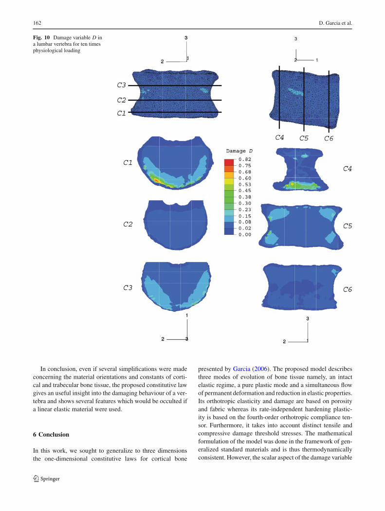
The simulation was run on a 8 processors SGI Origin 2000workstation. The computation required ten time increments.Within each increment, convergence of the projection algo-rithm was reached in one single iteration for the elastic modeand typically three iterations for the damaging mode. Inter-estingly, important damage values are strongly localized andaffect mainly the anterior trabecular bone elements which arenear the endplates (Fig. 10). This suggests that the contribu-tion of the trabecular bone to the total load depends on thelocation within the vertebra. Near the endplates, the trabecu-lar bone carries most of the load, whereas toward the middleof the vertebra the load is more evenly distributed betweenthe cortical shell and the trabecular bone. This result is con-firmed in the study of Liebschner et al. (2001). This strongand localized accumulation of damage may thus cause theanterior part of the vertebral body to crush, forming an ante-rior wedge fracture. Generally, ten times physiological load-ing happens only during extraordinary severe trauma suchas an automobile crash or a hard fall. However, we expectsimilar damage accumulation mechanisms and compressionfracture patterns at lower loads in cases of moderate or severeosteoporosis. A uniform distribution of the load within thevertebra is usually the case in healthy bones. Osteoporoticvertebrae exhibit an altered micro-architecture which couldresult in an uneven distribution of the load, facilitating local-ized damage.

123


Fig. 10 Damage variable D ina lumbar vertebra for ten timesphysiological loading

In conclusion, even if several simplifications were madeconcerning the material orientations and constants of corti-cal and trabecular bone tissue, the proposed constitutive lawgives an useful insight into the damaging behaviour of a ver-tebra and shows several features which would be occulted ifa linear elastic material were used.

6 Conclusion

In this work, we sought to generalize to three dimensionsthe one-dimensional constitutive laws for cortical bone

presented by Garcia (2006). The proposed model describesthree modes of evolution of bone tissue namely, an intactelastic regime, a pure plastic mode and a simultaneous flowof permanent deformation and reduction in elastic properties.Its orthotropic elasticity and damage are based on porosityand fabric whereas its rate-independent hardening plastic-ity is based on the fourth-order orthotropic compliance ten-sor. Furthermore, it takes into account distinct tensile andcompressive damage threshold stresses. The mathematicalformulation of the model was done in the framework of gen-eralized standard materials and is thus thermodynamicallyconsistent. However, the scalar aspect of the damage variable

123


restricts the applicability of the model to proportional loadingand unloading.

The numerical implementation of the three-dimensionallaw into a mechanical analysis software was done in astraightforward manner. Implicit (radial return) projectionalgorithms are used for plastic flow calculation and the gener-alized Newton method is used to overcome the nonlinearitiesassociated with damage evolution and hardening. Consistent(algorithmic) tangent operators are derived in order to ensurerapid convergence of the global Newton algorithm. Severalvalidation tests have proven the accuracy and convergenceof the final algorithm.

Finally, the biomechanical evaluation of a compressionof a human vertebra showed the potential of the proposedmodel. The same constitutive laws were used for corticaland trabecular bone, but with different porosities. The simu-lation results show a strong localization of damage within thetrabecular compartment which may cause the anterior part ofthe vertebral body to crush.

Acknowledgments This work was mainly supported by the SwissNational Science Foundation, Grant no. 32-6194400. The authors wouldlike to thank T. Kitzler (TU-WIEN) for providing the finite elementmesh of the lumbar vertebra.

Appendix

In order to find the incremental tangent operator, we mustfind the relation:

dS = Pad(∆E) (62)

where ∆E is the total strain increment. As S = S (E − Ep),we have:

dS = S d(∆E) − S d(∆Ep). (63)

The incremental flow rule to be linearized is:

∆Ep = λpNp(Sp) (64)

b) Plastic mode: case ∆Ep �= 0 and ∆D = 0

In that case, we find:

d(∆Ep) = dλp Np(Sp) + λpH

p(Sp) dSp (65)

As Sp = S E − 1D S Ep and ∆D = 0, we get:

dSp = S d(∆E) − 1

DS d(∆Ep) (66)

or with substitution of (65)

dSp = S d(∆E) − dλp

DS Np(Sp) − λp

DS H

p(Sp) dSp

(67)

or equivalently:

dSp = Sa d(∆E) − dλp

DSa Np(Sp) (68)

with Sa := [E + λp

D Hp(Sp)]−1. As S = Sp + SD , we have:

dS = dSp + dSD. (69)

Furthermore, as SD = 1−DD S Ep, we get:

dSD = 1 − D

DS d(∆Ep). (70)

From (63), we have:

S d(∆Ep) = S d(∆E) − dS, (71)

thus

dSD = 1 − D

DS [d(∆E) − E dS] . (72)

Combining with (69), we get:

dS = (1 − D) S d(∆E) + D dSp (73)

or with (68):

dS = (1 − D) S d(∆E) + D Sa d(∆E) − dλpSa Np(Sp).

(74)

As Y p(Sp, D) = 0, we have dY p = Np(Sp) : dSp = 0.Thus with (68):

dλp = DNp(Sp) : Sa d(∆E)

Np(Sp) : Sa Np(Sp). (75)

Using (74), we finally get the desired result:

dS =[

(1 − D) S

+D

(

Sa − Sa Np(Sp) ⊗ Sa Np(Sp)

Np(Sp) : Sa Np(Sp)

)]

d(∆E).

(76)

123


c) Damage mode: case ∆Ep �= 0 and ∆D �= 0

For conciseness of the presentation and as the method is verysimilar to case b), we only present the major changes withthat case.Instead of (66), we must write:

dSp = S d(∆E) − 1

DS d(∆Ep) + d(∆D)

D2 S Ep. (77)

Equation (70) becomes:

dSD = 1 − D

DS d(∆Ep) − d(∆D)

D2 S Ep. (78)

As Y D(SD, D) = 0 holds in that mode, we have:

dY D = ND(SD) : dSD + ∂Y D

∂ Dd(∆D) = 0. (79)

Combining (78) and (79), one gets an expression for d(∆D).The term dλp appearing in the linearization of the incremen-tal flow rule (65) can be found by making use of Y p(Sp, D) =0 i.e.

dY p = Np(Sp) : dSp + ∂Y p

∂ Dd(∆D) = 0. (80)

The incremental tangent operator presented in (57) is foundafter some algebraic rearrangements, cf. Garcia (2006).

References

Alart P, Curnier A (1991) A mixed formulation for frictional contactproblems prone to Newton like solution methods. Comput Meth-ods Appl Mech Eng 92:353–375

Ascenzi A, Bonucci E, Ripamonti A, Roveri N (1978) X-ray diffrac-tion and electron microscope study of osteons during calcification.Calcified Tissue Res 25:133–143

Cowin SC (1985) The relationship between the elasticity tensor and thefabric tensor. Mech Mater 4(2):137–147

Cowin SC (2001) Bone mechanics handbook, 2nd edn. CRC Press,Boca Raton

Curnier A (1993) Méthodes numériques en mécanique des solides.Presses Polytechniques et Universitaires Romandes (PPUR),Lausanne

Curnier A, He Q-C, Zysset PK (1995) Conewise linear elastic materi-als. J Elast 37:1–38

Currey JD (2002) Bones: structure and mechanics. Princeton Univer-sity Press, Princeton

Fondrk MT, Bahniuk EH, Davy DT, Michaels C (1988) Some visco-plastic characteristics of bovine and human cortical bone.J Biomech 21(8):623–630

Fondrk MT, Bahniuk EH, Davy DT (1999a) Inelastic strain accumu-lation in cortical bone during rapid transient tensile loading.J Biomech Eng 121:616–621

Fondrk MT, Bahniuk EH, Davy DT (1999b) A damage model for non-linear tensile behavior of cortical bone. J Biomed Eng 121:533–541

Garcia D (2006) Elastic plastic damage constitutive laws for cor-tical bone. PhD thesis, Ecole Polytechnique Fédérale de Lau-sanne (EPFL), Lausanne. Available online at: http://library.epfl.ch/theses/?nr=3435. Accessed 4 June 2007

Green AE, Naghdi PM (1965) A general theory of an elastic-plasticcontinuum. Arch Rational Mech Anal 18(4):251–281

Hansen NR, Schreyer HL (1994) A thermodynamically consistentframework for theories of elastoplasticity coupled with damage.Int J Solids Struct 31:359–389

He Q-C, Curnier A (1995) A more fundamental approach to damagedelastic stress-strain relations. Int J Solids Struct 32(10):1433–1457

Hill R (1950) The mathematical theory of plasticity. Oxford UniversityPress, London

Kanatani KI (1984) Distribution of directional data and fabric tensors.Int J Eng Sci 22(2):149–164

Keaveny TM, Wachtel EF, Kopperdahl DL (1999) Mechanical behaviorof human trabecular bone after overloading. J Orthop Res 17:346–353

Keaveny TM, Morgan EF, Niebur GL, Yeh OC (2001) Biomechanicsof trabecular bone. Annu Rev Biomed Eng 3:307–333

Kotha SP, Guzelsu N (2003) Tensile damage and its effects on corticalbone. J Biomech 36(11):1683–1689

Lemaitre J (1996) A course on damage mechanics, 2nd edn. Springer,New York

Lemaitre J, Chaboche JL (2001) Mécanique des matériaux solides, 2eédn. Dunod, Paris

Liebschner MAK, Kopperdahl DL, Rosenberg WS, Keaveny TM(2001) Contribution of cortical shell and endplate to vertebralbody stiffness. In: BED-Vol. 50, 2001 Bioengineering conference,ASME

Lubarda VA, Krajcinovic D (1995) Some fundamental issues in ratetheory of damage-elastoplasticity. Int J Plast 11:763–797

Moreau JJ (1979) Application of convex analysis to some problems ofdry friction. In: Zorski H (ed) Trends in applications of pure math-ematics to mechanics II. Pitman, London pp 263–280

Ortiz M (1985) A constitutive theory for the inelastic behavior of con-crete. Mech Mater 4(1):67–93

Prandtl L (1924) Spannungsverteilung in plastischen Körpern. In:Biezeno CB, J.M.B. (eds) Proceedings of the first interna-tional congress for applied mechanics. Technische Boekhandel enDruckerij, Waltman J Jr. Delft, pp 43–54

Rakotomanana RL, Curnier A, Leyvraz PF (1991) An objective aniso-tropic elastic plastic model and algorithm applicable to bonemechanics. Eur J Mech A/Solids 10(3):327–342

Reuss A (1930) Berücksichtigung der elastischen Formänderung inder Plastizitätstheorie. Zeitschrift Angewandte Math Mech 10:266–274

Rho J-Y, Kuhn-Spearing L, Zioupos P (1998) Mechanical propertiesand the hierarchical structure of bone. Med Eng Phys 20(2):92–102

Rincón L (2003) Identification of a multiaxial failure criterion for humantrabecular bone. PhD thesis, Ecole Polytechnique Fédérale deLausanne (EPFL), Lausanne. Available online at: http://library.epfl.ch/theses/?nr=2812. Accessed 4 June 2007

Rockafellar RT (1970) Convex analysis. Princeton University Press,Princeton

Simo JC, Taylor RL (1985) Consistent tangent operators for rate-independent elastoplasticity. Comput Methods Appl Mech Eng48(1):101–118

Simo JC, Hughes TJR (1999) Computational inelasticity. Springer,Berlin

Timoshenko S (1968) Résistance des matériaux, vol 2. Dunod, ParisWilkins ML (1964) Calculation of elastic-plastic flow. Methods

Comput Phys 3:211–263Ziegler H (1983) An introduction to thermomechanics, 2nd edn. North-

Holland, Amsterdam

123

http://library.epfl.ch/theses/?nr=3435





Zysset P (1994) A constitutive law for trabecular bone. PhD thesis, EcolePolytechnique Fédérale de Lausanne (EPFL), Lausanne. Availableonline at: http://library.epfl.ch/theses/?nr=1252. Accessed 4 June2007

Zysset PK, Curnier A (1996) An implicit projection algorithm forsimultaneous flow of plasticity and damage in standard generalizedmaterials. Int J Numer Methods Eng 39:3065–3082

Zysset PK, Curnier A (1995) An alternative model for anisotropicelasticity based on fabric tensors. Mech Mater 21(4):243–250

Zysset PK (2003) A review of morphology-elasticity relationships inhuman trabecular bone: theories and experiments. J Biomech36:1469–1485

Zysset PK, Rincón L (2006) An alternative fabric-based yield and fail-ure criterion for trabecular bone. In: Holzapfel GA, Ogden RW(eds) Mechanics of biological tissue. Springer, Berlin pp 457–470

123


Documents

3D Konstituvne Relacije Za Kost