3D imaging of Mars’ polar ice caps using orbital radar data imaging of Mars’ polar ice caps using orbital radar data ... to date is NASA’s Mars Reconnaissance Orbiter (MRO) mission,

Special Section: Remote sensing January 2017 THE LEADING EDGE 43

3D imaging of Mars’ polar ice caps using orbital radar data

AbstractSince its arrival in early 2006, various instruments aboard

NASA’s Mars Reconnaissance Orbiter (MRO) have been col-lecting a variety of scientific and engineering data from orbit around Mars. Among these is the Shallow Radar (SHARAD) instrument, supplied by Agenzia Spaziale Italiana (ASI) and designed for subsurface sounding in the 15–25 MHz frequency band. As of this writing, MRO has completed more than 46,000 nearly polar orbits of Mars, 30% of which have included active SHARAD data collection. By 2009, a sufficient density of SHA-RAD coverage had been obtained over the polar regions to support 3D processing and analysis of the data. Using tools and techniques commonly employed in terrestrial seismic data processing, we have processed subsets of the resulting collection of SHARAD observations covering the north and south polar regions as SHA-RAD 3D volumes, imaging the interiors of the north and south polar ice caps known, respectively, as Planum Boreum and Planum Australe. After overcoming a series of challenges revealed during the 3D processing and analysis, a completed Planum Boreum 3D volume is being used currently for scientific research. Lessons learned in the northern work fed forward into our 3D processing and analysis of the Planum Australe 3D volume, currently under way. We discuss our experiences with these projects and present results and scientific insights stemming from these efforts.

IntroductionThe exploration of other planets in our solar system has been

a dream of humankind since ancient times. Modern space explora-tion has turned that dream into reality through the successful building, launch, and delivery of spacecraft to fly by, orbit, or land on every planetary body in the solar system. For no other planet has there been more of this remote exploration than for Mars, with some 44 Mars missions launched worldwide since 1960 and 21 of these successful to some degree. Among the most successful to date is NASA’s Mars Reconnaissance Orbiter (MRO) mission, which launched in August 2005, entered orbit around Mars in March 2006, and began collecting scientific observations in November 2006 (Zurek and Smrekar, 2007). After orbit insertion and aerobraking, the spacecraft was placed into a subpolar (87.4° inclination) and near-circular (ranging from 250 to 316 km eleva-tion, with periapsis near the south pole) orbit of ~112 minutes in duration. MRO’s observation coverage of the planet’s surface has grown steadily during the more than 46,000 orbits completed as of the time of this writing. MRO carries six science instruments, including three cameras (HiRISE, the High Resolution Imaging Science Experiment; CTX, the Context Camera; and MARCI, the Mars Color Imager), a spectrometer (CRISM, the Compact Reconnaissance Imaging Spectrometer for Mars), a radiometer

Frederick J. Foss II1, Nathaniel E. Putzig2, Bruce A. Campbell3, and Roger J. Phillips4

(MCS, the Mars Climate Sounder), and a radar sounder (SHA-RAD, the Shallow Radar).

The scientific observations and data provided by these instru-ments have directly led to significant discoveries about the geologi-cal and climatological histories of Mars. Apart from major SHARAD-related findings in the polar regions (discussed later), some of the most important MRO discoveries, sorted roughly by the geologic time period to which they apply, include:

• MRO data provide evidence that the Tharsis volcanic plateau is underlain by part of an enormous elliptical basin, suggesting that the hemispheric dichotomy (northern lowlands versus southern highlands) is the result of a giant impact very early in Martian history (Andrews-Hanna et al., 2008).

• MRO data indicate that ancient impacts produced extensive glass, which has important implications for early cratering rates and habitability (Schultz et al., 2015).

• MRO found evidence that hydrothermal alteration occurred at regionally variable depths, and that older crust at greater depths was intruded by plutons (Wray et al., 2013). In addition, new evidence has been found for fluvial/volcanic interactions in the shallow crust (Dundas and Keszthelyi, 2013).

• A broad diversity of ancient environments has been revealed through detection of carbonates, exhumed hydrothermal deposits, and the spatial density of aqueous deposits. The data show that liquid water was once at and near the surface and that differing environments (wet/neutral or dry/acidic) did not evolve over time in a smooth progression but instead may have occurred repeatedly or coexisted in adjacent locations (Ehlmann and Edwards, 2014).

• Remnant debris-covered glaciers and other near-surface ices in the mid-latitudes have been discovered and characterized with MRO data. These features provide a record of past cli-mates when ice was accumulating in these areas during times of higher obliquity (tilt of the planet’s spin axis) (Holt et al., 2008; Plaut et al., 2009).

• The discovery of recurring slope lineae (RSL) suggests that seepage of water is occurring seasonally today (McEwen et al., 2014). Within the RSL, observed changes in hydrated perchlorates provide support to flowing brines as the RSL source (Ojha et al., 2015).

• MRO has identified hundreds of new impact craters emplaced during the course of the mission, adding new data on the present-day cratering rate at Mars. Many such impacts have exposed water ice, extending the boundary of shallow ice closer to the equator in both hemispheres than inferred previously from thermal and neutron spectrometer data (Dundas et al., 2014).

1Freestyle Analytical & Quantitative Services, LLC.2Planetary Science Institute.3Smithsonian Institution.4Department of Earth and Planetary Sciences and McDonnell Center

for the Space Sciences, Washington University in St. Louis.

http://dx.doi.org/10.1190/tle36010043.1.

Special Section: Remote sensing44 THE LEADING EDGE January 2017

• MRO has discovered and characterized nonuniform distribu-tions of dust and ice clouds in the atmosphere, which have been found to give rise to many of the observed circulation features in the Martian atmosphere (Heavens et al., 2011).

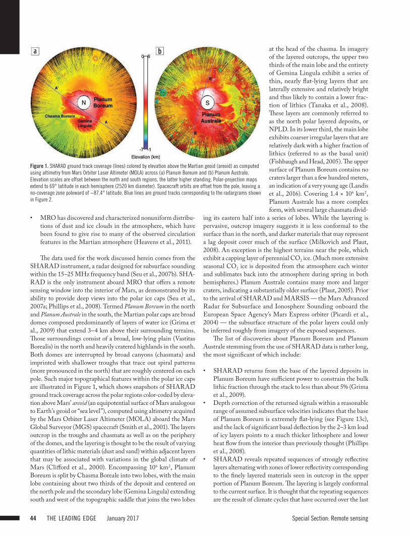
The data used for the work discussed herein comes from the SHARAD instrument, a radar designed for subsurface sounding within the 15–25 MHz frequency band (Seu et al., 2007b). SHA-RAD is the only instrument aboard MRO that offers a remote sensing window into the interior of Mars, as demonstrated by its ability to provide deep views into the polar ice caps (Seu et al., 2007a; Phillips et al., 2008). Termed Planum Boreum in the north and Planum Australe in the south, the Martian polar caps are broad domes composed predominantly of layers of water ice (Grima et al., 2009) that extend 3–4 km above their surrounding terrains. Those surroundings consist of a broad, low-lying plain (Vastitas Borealis) in the north and heavily cratered highlands in the south. Both domes are interrupted by broad canyons (chasmata) and imprinted with shallower troughs that trace out spiral patterns (more pronounced in the north) that are roughly centered on each pole. Such major topographical features within the polar ice caps are illustrated in Figure 1, which shows snapshots of SHARAD ground track coverage across the polar regions color-coded by eleva-tion above Mars’ areoid (an equipotential surface of Mars analogous to Earth’s geoid or “sea level”), computed using altimetry acquired by the Mars Orbiter Laser Altimeter (MOLA) aboard the Mars Global Surveyor (MGS) spacecraft (Smith et al., 2001). The layers outcrop in the troughs and chasmata as well as on the periphery of the domes, and the layering is thought to be the result of varying quantities of lithic materials (dust and sand) within adjacent layers that may be associated with variations in the global climate of Mars (Clifford et al., 2000). Encompassing 106 km2, Planum Boreum is split by Chasma Boreale into two lobes, with the main lobe containing about two thirds of the deposit and centered on the north pole and the secondary lobe (Gemina Lingula) extending south and west of the topographic saddle that joins the two lobes

at the head of the chasma. In imagery of the layered outcrops, the upper two thirds of the main lobe and the entirety of Gemina Lingula exhibit a series of thin, nearly flat-lying layers that are laterally extensive and relatively bright and thus likely to contain a lower frac-tion of lithics (Tanaka et al., 2008). These layers are commonly referred to as the north polar layered deposits, or NPLD. In its lower third, the main lobe exhibits coarser irregular layers that are relatively dark with a higher fraction of lithics (referred to as the basal unit) (Fishbaugh and Head, 2005). The upper surface of Planum Boreum contains no craters larger than a few hundred meters, an indication of a very young age (Landis et al., 2016). Covering 1.4 × 106 km2, Planum Australe has a more complex form, with several large chasmata divid-

ing its eastern half into a series of lobes. While the layering is pervasive, outcrop imagery suggests it is less conformal to the surface than in the north, and darker materials that may represent a lag deposit cover much of the surface (Milkovich and Plaut, 2008). An exception is the highest terrains near the pole, which exhibit a capping layer of perennial CO2 ice. (Much more extensive seasonal CO2 ice is deposited from the atmosphere each winter and sublimates back into the atmosphere during spring in both hemispheres.) Planum Australe contains many more and larger craters, indicating a substantially older surface (Plaut, 2005). Prior to the arrival of SHARAD and MARSIS — the Mars Advanced Radar for Subsurface and Ionosphere Sounding onboard the European Space Agency’s Mars Express orbiter (Picardi et al., 2004) — the subsurface structure of the polar layers could only be inferred roughly from imagery of the exposed sequences.

The list of discoveries about Planum Boreum and Planum Australe stemming from the use of SHARAD data is rather long, the most significant of which include:

• SHARAD returns from the base of the layered deposits in Planum Boreum have sufficient power to constrain the bulk lithic fraction through the stack to less than about 5% (Grima et al., 2009).

• Depth correction of the returned signals within a reasonable range of assumed subsurface velocities indicates that the base of Planum Boreum is extremely flat-lying (see Figure 13c), and the lack of significant basal deflection by the 2–3 km load of icy layers points to a much thicker lithosphere and lower heat flow from the interior than previously thought (Phillips et al., 2008).

• SHARAD reveals repeated sequences of strongly reflective layers alternating with zones of lower reflectivity corresponding to the finely layered materials seen in outcrop in the upper portion of Planum Boreum. The layering is largely conformal to the current surface. It is thought that the repeating sequences are the result of climate cycles that have occurred over the last

Figure 1. SHARAD ground track coverage (lines) colored by elevation above the Martian geoid (areoid) as computed using altimetry from Mars Orbiter Laser Altimeter (MOLA) across (a) Planum Boreum and (b) Planum Australe. Elevation scales are offset between the north and south regions, the latter higher standing. Polar-projection maps extend to 69° latitude in each hemisphere (2520 km diameter). Spacecraft orbits are offset from the pole, leaving a no-coverage zone poleward of ~87.4° latitude. Blue lines are ground tracks corresponding to the radargrams shown in Figure 2.


4 million years of Martian history (Phillips et al., 2008; Putzig et al., 2009). A shallow unconformity seen in SHARAD data appears to correspond to a suspected retreat from an episode of midlatitude glaciation 370,000 years ago (Smith et al., 2016).

• Mapping of layering unconformities in SHARAD data shows that Chasma Boreale is a center of near-zero net deposition rather than an erosional feature, having developed in conjunction with variable deposition rates across the region. In contrast, a paleo-chasma of similar size to Chasma Boreale that existed early in Planum Boreum history appears to have been infilled, leaving no appreciable surface expres-sion (Holt et al., 2010).

• Below the spiral troughs in Planum Boreum, layering dis-continuities in SHARAD data extend downward, often to several hundred meters depth. These trough-bounding surfaces map out a poleward progression of the troughs over time while demonstrating that the troughs form largely as a result of aeolian erosion of water ice from their steeper poleward slopes and redeposition on their shallower equatorward slopes (Smith and Holt, 2010).

• While SHARAD also reveals layering sequences beneath Planum Australe, they have characteristics distinct from those in the north, including truncation very near the surface in many locations (Seu et al., 2007a), and the signal-to-noise (S/N) ratio at depth is often attenuated, perhaps due to a broadly distributed scatterer in the near-surface (Campbell et al., 2015).

• SHARAD data show several regions in Planum Australe near the south pole that contain materials with extremely low reflectivity (see Figures 11a and 11b). These deposits have been shown to be made up of nearly pure CO2 ice, containing enough material to double Martian atmospheric pressure if sublimated (Phillips et al., 2011). The deposits occur in three layers that likely correspond to episodes of atmospheric collapse during times of low obliquity extending back at least 370,000 years, each capped by a ~30 m layer of water ice sufficient to prevent sublimation of the CO2 in subsequent returns to higher obliquity (Bierson et al., 2016).

The SHARAD instrument transmits and receives via a 10 m dipole antenna, emitting a 10 W linearly down-swept chirp from 25 to 15 MHz over 85.05 μs at a pulse repetition frequency (PRF) of 700.28 Hz. The terrain-following receive window is 135 μs in duration, within which the returned radar signal is sampled at a rate of 37.5 ns, giving a total of 3600 voltage samples per radar frame (analogous to a trace in the seismic realm). Note that the sampling frequency (26.66 MHz) gives a fundamental frequency range of 0–13.33 MHz, which means that the non-baseband signal spectrum is fully aliased upon sampling. With these parameters and the spacecraft’s altitude and velocity, SHARAD samples any target within the 20.25 km range window with a 3–6 km Fresnel zone at the surface (improvable with Doppler processing along-track to 0.3–1 km) and 15/√εr m along range (so 15 m in free space and lower within the ice caps de-pending on the real dielectric constant εr). For further details about SHARAD and its counterpart MARSIS, see (Picardi et al., 2004; Seu et al., 2007b).

Over time, as the planet has rotated below (rotational period is 24 hours and 37 minutes), the nearly polar orbit of MRO has resulted in relatively dense coverage (when compared with the rest of the planet) of the polar regions with SHARAD observa-tions. After years of mapping and analysis using collections of SHARAD data from individual orbit passes, it became clear that the structural complexity of the polar ice caps was sufficient to merit 3D treatment of the SHARAD data. In 2010, after the SHARAD coverage density over the poles became sufficient to support 3D processing, we began work on the north polar SHA-RAD 3D project. At that time, we limited our effort to about 500 observations (data collected continuously over a given orbit segment) distributed across Planum Boreum, but we later expanded the coverage to a final count of more than 2300 observations. We further expanded our efforts in 2013 with another SHARAD 3D project for Planum Australe. These two projects have resulted in the first high-fidelity 3D images of the interiors of Mars’ polar ice caps, samples of which we include herein.

SHARAD preprocessingBefore application of 3D processing, the recorded (2D) SHA-

RAD data has undergone both onboard processing and Earth-based processing (Campbell and Phillips, 2014). The onboard processing simply consists of coherent (with respect to the so-called Doppler bandwidth) summation of radar frames, typically by a factor of eight for this data set, to reduce the data volume transmit-ted to Earth. The processing on Earth consists of:

1) Range compression (Campbell et al., 2011): cross correlation of each radar frame with a model of the transmitted chirp. The chirp’s phase is modified with an estimate of the ionospheric phase distortion modeled via a focusing metric derived from the data, thereby approximately removing the significant effects on the data of the signal’s passage through the Martian ionosphere. This process is implemented in the frequency domain, after which the redundant half of the spectrum is set to zero and the result is inverse Fourier transformed to obtain the corresponding (complex) analytic signal.

2) Synthetic Aperture Radar (SAR) processing: the range-com-pressed analytic data are assembled into a complex 2D pro-cessing array (the synthetic aperture, with a predetermined set of frames comprising the columns of the array) and the following operations are performed relative to the center location within the aperture resulting in an along-track focus-ing of the data:a) Range migration: up-range shifting of frames to align returns

from the surface at the synthetic aperture center.b) Doppler shift correction: frequency-dependent, location-

dependent along-track phase rotation to correct the Doppler shift caused by the relative motion of the space-craft and synthetic aperture center.

c) Coherent summation: to increase the S/N, iso-range delay samples along rows in the synthetic aperture are Fourier transformed and the total power in the spectrum com-puted and output at each time delay index to form each output frame, the collection of such frames along-track comprising the so-called “radargram.”


3) Residual ionospheric time delays correction (Campbell et al., 2014):a) Residual ionospheric time delays revealed and modeled

as a linear regression between differential time delays and corresponding differential ionospheric distortion parameter values (derived in Step 1) measured using colocated frames from different observations within high-latitude, high-fold “gathers” (see discussion below).

b) Corrections applied to every frame through a polynomial fit of the derived differential time delays against solar zenith angle (SZA) for every frame.

4) Datuming: the radargram is datumed to 10,125 m above Mars’ areoid.

Every such radargram and its processing description using the aforementioned preprocessing workflow are available in NASA’s Planetary Data System (PDS) archive (Campbell and Phillips, 2014). Note that we widened the Doppler bandwidth (used in Step 2b above) for the radargrams used in 3D processing over that used for the radargrams delivered to the PDS, as we found that doing so better preserved radar returns with steeper slopes. It is important to emphasize that Step 3 in this preprocessing workflow

is a direct consequence of the analysis of a set of high-latitude, high-fold “gathers” (quotes to indicate that the data is zero-offset, so there is no offset distribution typical of terrestrial seismic gathers), each composed of frames taken from different radargrams falling within a common spatial bin. Because the ionosphere is a sun-driven dynamic distortion medium for any electromagnetic signal above its plasma frequency5, radargrams sufficiently sepa-rated in their acquisition timing are likely to be affected differently by the ever-changing ionosphere, including with respect to their relative signal phases at crossover locations. The gather analysis revealed such residual relative ionospheric time delays that there-tofore had not been assessed in individual radargrams, thereby providing valuable feedback that has benefited the SHARAD preprocessing workflow.

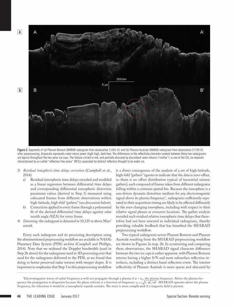
Two typical radargrams across Planum Boreum and Planum Australe resulting from the SHARAD preprocessing workflow are shown in Figures 2a resp. 2b. In scrutinizing and comparing these observations, the SHARAD signal character difference between the two ice caps is rather apparent, with Planum Boreum returns having a higher S/N and more subsurface reflection in-terfaces, including a distinct basal reflection event. The interior reflectivity of Planum Australe is more sparse and obscured by

5Electromagnetic waves of radial frequency ω will not propagate through a plasma if ω < ωp, the plasma frequency. Above the plasma fre-quency the propagation is dispersive because the phase velocity is a function of frequency v0 = c0 1−ω p

2 /ω 2 . SHARAD operates above the plasma frequency, for otherwise it would be a ionospheric topside sounder. The story is more complicated if a magnetic field is present.

Figure 2. Segments of (a) Planum Boreum SHARAD radargram from observation 11301-01 and (b) Planum Australe SHARAD radargram from observation 27199-01 after preprocessing. Grayscale represents radar return power (light high, dark low). The differences in the reflectivity character evident between these two radargrams are typical throughout the two polar ice caps. The feature circled in red, and partially obscured by discordant radar returns (“clutter”), is one of the CO2 ice deposits characterized by so-called “reflection free zones” (RFZs) separated by distinct reflectors thought to be water ice.


relatively high-power background noise informally referred to as “fog” (Campbell et al., 2015). One particular subsurface feature (circled in red) is a wedge-shaped CO2 deposit characterized by three layers having no internal reflectivity, so-called “reflection free zones” (RFZs), and separated by distinct bright reflectors (Phillips et al., 2011). This feature is rather obscured in this 2D preprocessed radargram by radar returns that have not been properly handled by the 2D preprocessing outlined above (thus it appears as “clutter” in the radargram). We’ll see later that this feature is clarified quite remarkably after 3D processing.

3D processing and analysis of SHARAD dataWe have developed and applied 3D processing and analysis

workflows to more than 4400 SHARAD radargrams initially processed as those shown in Figure 2, about 2300 covering Planum Boruem in the north and about 2100 covering Planum Australe in the south. This effort has resulted in the first fully 3D processed orbital radar volumes in history, and the revelations and lessons learned from examining and analyzing the data used to produce these volumes have been and continue to be fed forward to produce better radargrams and thus better 3D volumes in ever shorter turn-around times. To produce these 3D volumes, the rather large respec-tive collections of radargrams covering each pole were assigned map coordinates in an appropriate polar projection system, rectilinearly binned, and 3D processed and imaged. To manage these large 3D data sets and to leverage existing technology, we used Landmark Graphics Corporation’s ProMAX/SeisSpace for the 3D processing and SeisWare’s interpretation software. This crossover of terrestrial seismic exploration technology into the realm of extraterrestrial orbital radar is novel and has proven to be very successful.

While the 2D preprocessing previously described is more or less standard in the realm of orbital radar, the resulting radargrams are not entirely suitable for immediate use in 3D processing. Specifi-cally, the range migration step is undesirable prior to 3D processing since it is essentially a 2D migration along the ground track of each observation. This is only a partial migration in a 3D structural setting, and since all the ground tracks over the poles have a full range of azimuths, the only practical way to accommodate this step is to reverse it to the extent possible with the application of a 2D demigration of each radargram followed by a full 3D migration of the 3D volume of demigrated data. Also, processing radargrams whose radar return samples are power-valued rather than ampli-tude-valued is not ideal, but, for a variety of reasons, unwinding this step from the other SAR processing steps is complicated and we chose not to attempt it for these initial projects. For Planum Boreum data, we simply used the radar return power while for Planum Australe data, we took the square root of the power-valued samples to convert them to so-called reflection strength (Taner et al., 1979) as doing so better accommodated the lower S/N, debiasing each frame prior to subsequent 3D processing.

In preparation for 3D processing, the following 2D processing workflow was applied to every 2D preprocessed radargram:

1) Redatuming: use the spacecraft and areoid radii to reverse the range delay windowing and areoid reference datuming imposed during SAR processing and thereby restore the radar signal timing to its original orbit datum range delay timing.

2) Demigration: approximately reverse the along-track range migration performed during SAR processing.

3) Common reference datuming: remove the intra- and interorbital variation in spacecraft altitude, thereby referencing to a common constant orbit radius datum derived as the average spacecraft orbit radius taken over a representative subset of the radargrams used for 3D processing.

4) Bulk shift: strip away most of the traveltime above the first returns for storage efficiency by applying a constant negative time shift and truncating every frame commensurately.

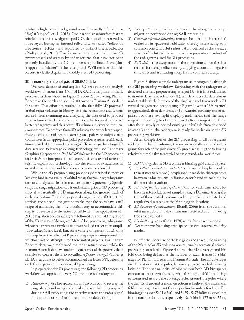
Figure 3 shows a single radargram as it progresses through this 2D processing workflow. Beginning with the radargram as delivered after 2D preprocessing as input (3a), it is first redatumed to its orbit delay time reference (3b), which renders the data almost undetectable at the bottom of the display panel (even with a 7:1 vertical exaggeration, reappearing in Figure 3c with a 272:1 vertical exaggeration), then demigrated (3d). Careful scrutiny and com-parison of these two right display panels shows that the range migration focusing has been removed after demigration. Then, after the relatively minor redatuming and bulk shifting described in steps 3 and 4, the radargram is ready for inclusion in the 3D processing workflow.

After completion of the 2D processing of all radargrams included in the 3D volumes, the respective collections of radar-grams for each of the poles were 3D processed using the following relatively simple (by terrestrial seismic standards) workflow:

1) 3D binning: define 3D rectilinear binning grid and bin space.2) 3D reflection correlation autostatics: derive and apply intra-bin

trim statics to remove (unexplained) time delay discrepancies between radar returns in frames contributed to each bin by different observations.

3) 3D interpolation and regularization: for each time slice, bi-linearly interpolate input samples using a Delaunay triangula-tion of their spatial locations and output the interpolated and regularized samples at the binning grid locations.

4) 3D downward continuation (Biondi, 2006) from the common orbit radius datum to the maximum areoid radius datum using free space velocity.

5) 3D Stolt migration (Stolt, 1978) using free space velocity.6) Depth conversion using free space-ice cap interval velocity

model.

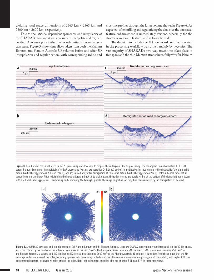
But for the sheer size of the bin grids and spaces, the binning of the Mars polar 3D volumes was routine by terrestrial seismic processing standards. Figure 4 shows the 3D coverage and bin fold (fold being defined as the number of radar frames in a bin) maps for Planum Boreum and Planum Australe. The 3D coverages are densest nearest the poles, becoming sparser with decreasing latitude. The vast majority of bins within both 3D bin spaces contain at most two frames, with the higher fold bins being concentrated nearest the coverage holes around the poles where the density of ground track intersections is highest, the maximum folds reaching 51 resp. 64 frames per bin for only a few bins. The binning grids span 5401 × 5401 and 5475 × 5475 inlines × crosslines in the north and south, respectively. Each bin is 475 m × 475 m,


yielding total space dimensions of 2565 km × 2565 km and 2600 km × 2600 km, respectively.

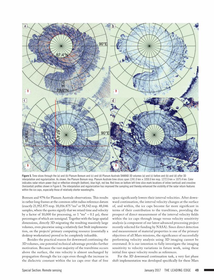
Due to the latitude-dependent sparseness and irregularity of the SHARAD coverage, it was necessary to interpolate and regular-ize the 3D volumes prior to the downward continuation and migra-tion steps. Figure 5 shows time slices taken from both the Planum Boreum and Planum Australe 3D volumes before and after 3D interpolation and regularization, with corresponding inline and

crossline profiles through the latter volume shown in Figure 6. As expected, after infilling and regularizing the data over the bin space, feature enhancement is immediately evident, especially for the shorter wavelength features and at lower latitudes.

The decision to include the 3D downward continuation step in the processing workflow was driven mainly by necessity. The vast majority of SHARAD’s two-way traveltime takes place in free space and the thin Martian atmosphere, fully 98% for Planum

Figure 3. Results from the initial steps in the 2D processing workflow used to prepare the radargrams for 3D processing. The radargram from observation 11301-01 across Planum Boreum (a) immediately after SAR processing (vertical exaggeration 242:1), (b) and (c) immediately after redatuming to the observation’s original orbit datum (vertical exaggerations 7:1 resp. 272:1), and (d) immediately after demigration at this same datum (vertical exaggeration 272:1). Color indicates radar return power (blue high, red low). After redatuming the input radargram back to its orbit datum, the radar returns are barely visible at the bottom of the lower left panel (even with a 7:1 vertical exaggeration). Scrutinizing and comparing the two right panels, the range migration focusing has been removed by the demigration as desired.

Figure 4. SHARAD 3D coverage and bin fold maps for (a) Planum Boreum and (b) Planum Australe. Lines are SHARAD observation ground tracks within the 3D bin space, each bin colored by the number of radar frames contained in the bin (“fold”). The bin space dimensions are 5401 inlines × 5401 crosslines spanning 2565 km2 for the Planum Boreum 3D volume and 5475 inlines × 5475 crosslines spanning 2600 km2 for the Planum Australe 3D volume. It is evident from these maps that the 3D coverage is densest nearest the poles, becoming sparser with decreasing latitude, and the 3D volumes are overwhelmingly single and double fold, with higher fold bins concentrated nearest the coverage holes around the poles. Note that inline resp. crossline bins are oriented S-N resp. E-W in these map views.


Figure 5. Time slices through the (a) and (b) Planum Boreum and (c) and (d) Planum Australe SHARAD 3D volumes (a) and (c) before and (b) and (d) after 3D interpolation and regularization. As shown, the Planum Boreum resp. Planum Australe time slices span 1241.0 km × 1050.0 km resp. 1272.0 km × 1075.4 km. Color indicates radar return power (top) or reflection strength (bottom), blue high, red low. Red lines on bottom left time slice mark locations of inline (vertical) and crossline (horizontal) profiles shown in Figure 6. The interpolation and regularization has improved the sampling and thereby enhanced the visibility of the radar return features within the ice caps, especially those of relatively shorter wavelengths.

Boreum and 97% for Planum Australe observations. This results in rather long frames at the common orbit radius reference datum (exactly 21,952.875 resp. 18,016.875 “ms” or 58,542 resp. 48,046 samples, where the quotes signify that we retard time and velocity by a factor of 10,000 for processing, so 1 “ms” = 0.1 μs), these percentages of which are nonsignal. Together with the large spatial dimensions, directly 3D migrating the resulting massively large volumes, even piecewise using a relatively fast Stolt implementa-tion, on the projects’ primary computing resource (essentially a desktop workstation) proved to be completely infeasible.

Besides the practical reason for downward continuing the 3D volumes, one potential technical advantage provides further motivation. Because the vast majority of the traveltime occurs above the surface, the rms velocity is almost unchanged by propagation through the ice caps even though the increase in the dielectric constant within the ice caps over that of free

space significantly lowers their interval velocities. After down-ward continuation, the interval velocity changes at the surface of, and within, the ice caps become far more significant in terms of their contribution to the traveltimes, providing the prospect of direct measurement of the interval velocity fields within the ice caps through image versus velocity sensitivity analysis (a component of our latest advanced processing project recently selected for funding by NASA). Since direct detection and measurement of material properties is one of the primary objectives of all Mars missions, the significance of successfully performing velocity analysis using 3D imaging cannot be overstated. It is our intention to fully investigate the imaging sensitivity to velocity variations in future work, using these initial free space velocity results as references.

For the 3D downward continuation task, a very fast phase shift implementation was developed specifically for these Mars


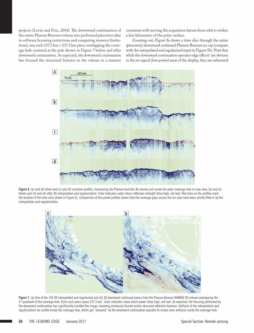
Figure 6. (a) and (b) Inline and (c) and (d) crossline profiles, transecting the Planum Australe 3D volume just inside the polar coverage hole in map view, (a) and (c) before and (b) and (d) after 3D interpolation and regularization. Color indicates radar return reflection strength (blue high, red low). Red lines on the profiles mark the location of the time slice shown in Figure 5c. Comparison of the paired profiles shows that the coverage gaps across the ice caps have been mostly filled in by the interpolation and regularization.

Figure 7. (a) One of the 144 3D interpolated and regularized and (b) 3D downward continued pieces from the Planum Boreum SHARAD 3D volume overlapping the 3rd quadrant of the coverage hole. Each such piece spans 237.5 km2. Color indicates radar return power (blue high, red low). As expected, the focusing performed by the downward continuation has significantly clarified the image, revealing previously blurred and/or obscured reflection features. Artifacts of the interpolation and regularization are visible inside the coverage hole, which get “smeared” by the downward continuation operator to create more artifacts inside the coverage hole.

projects (Levin and Foss, 2014). The downward continuation of the entire Planum Boreum volume was performed piecewise (due to software licensing restrictions and computing resource limita-tions), one such 237.5 km × 237.5 km piece overlapping the cover-age hole centered at the pole shown in Figure 7 before and after downward continuation. As expected, the downward continuation has focused the structural features in the volume in a manner

consistent with moving the acquisition datum from orbit to within a few kilometers of the polar surface.

Zooming out, Figure 8a shows a time slice through the entire (piecewise) downward continued Planum Boreum ice cap (compare with the interpolated and regularized input in Figure 5b). Note that while the downward continuation operator edge effects6 are obvious in the no-signal (low power) areas of the display, they are subsumed


6Parameter testing revealed these can be eliminated by increasing the inline and crossline overlap between adjacent pieces by a factor of 3, but at a rather significant premium of 5–6 times more compute time.

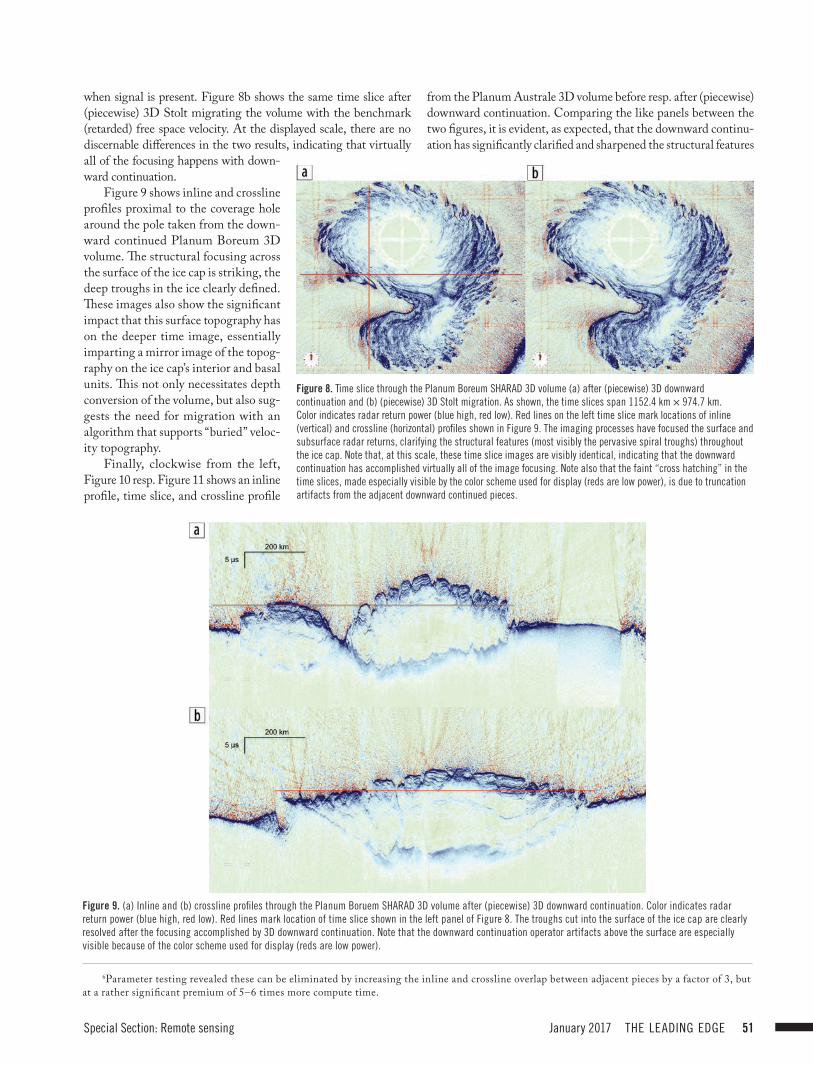
Figure 8. Time slice through the Planum Boreum SHARAD 3D volume (a) after (piecewise) 3D downward continuation and (b) (piecewise) 3D Stolt migration. As shown, the time slices span 1152.4 km × 974.7 km. Color indicates radar return power (blue high, red low). Red lines on the left time slice mark locations of inline (vertical) and crossline (horizontal) profiles shown in Figure 9. The imaging processes have focused the surface and subsurface radar returns, clarifying the structural features (most visibly the pervasive spiral troughs) throughout the ice cap. Note that, at this scale, these time slice images are visibly identical, indicating that the downward continuation has accomplished virtually all of the image focusing. Note also that the faint “cross hatching” in the time slices, made especially visible by the color scheme used for display (reds are low power), is due to truncation artifacts from the adjacent downward continued pieces.

Figure 9. (a) Inline and (b) crossline profiles through the Planum Boruem SHARAD 3D volume after (piecewise) 3D downward continuation. Color indicates radar return power (blue high, red low). Red lines mark location of time slice shown in the left panel of Figure 8. The troughs cut into the surface of the ice cap are clearly resolved after the focusing accomplished by 3D downward continuation. Note that the downward continuation operator artifacts above the surface are especially visible because of the color scheme used for display (reds are low power).

when signal is present. Figure 8b shows the same time slice after (piecewise) 3D Stolt migrating the volume with the benchmark (retarded) free space velocity. At the displayed scale, there are no discernable differences in the two results, indicating that virtually all of the focusing happens with down-ward continuation.

Figure 9 shows inline and crossline profiles proximal to the coverage hole around the pole taken from the down-ward continued Planum Boreum 3D volume. The structural focusing across the surface of the ice cap is striking, the deep troughs in the ice clearly defined. These images also show the significant impact that this surface topography has on the deeper time image, essentially imparting a mirror image of the topog-raphy on the ice cap’s interior and basal units. This not only necessitates depth conversion of the volume, but also sug-gests the need for migration with an algorithm that supports “buried” veloc-ity topography.

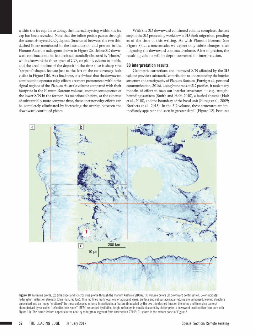
Finally, clockwise from the left, Figure 10 resp. Figure 11 shows an inline profile, time slice, and crossline profile

from the Planum Australe 3D volume before resp. after (piecewise) downward continuation. Comparing the like panels between the two figures, it is evident, as expected, that the downward continu-ation has significantly clarified and sharpened the structural features


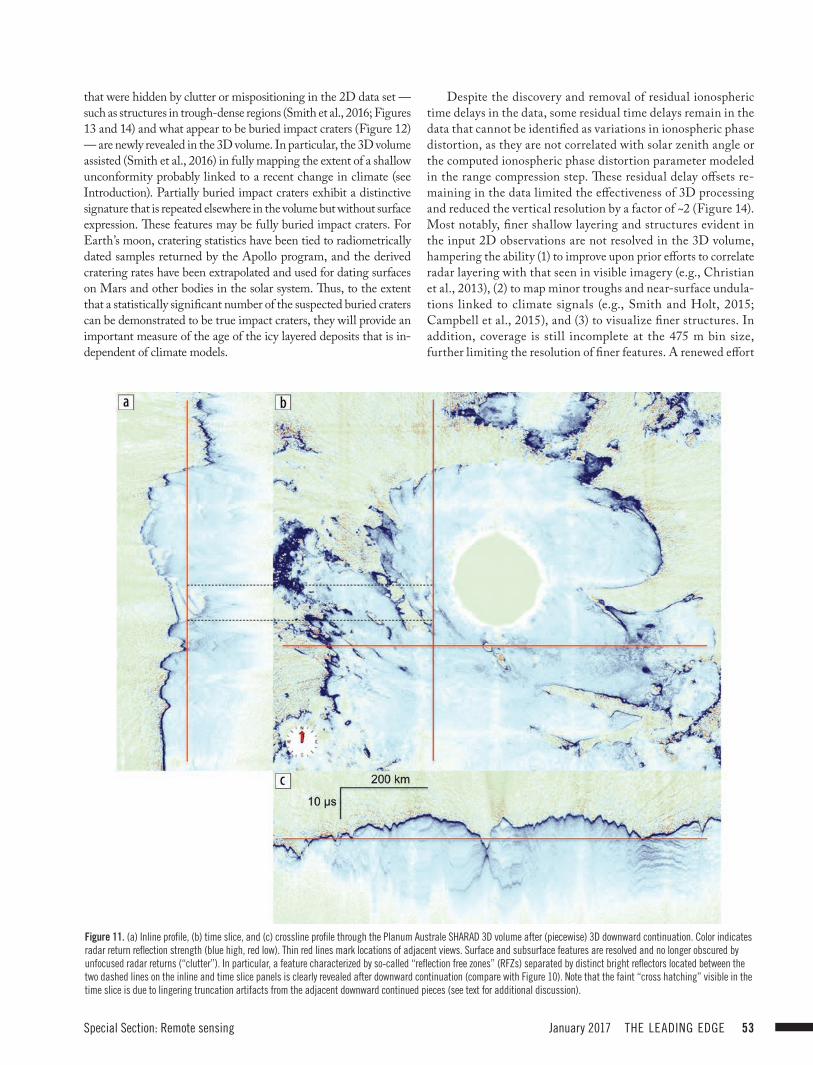
within the ice cap. In so doing, the internal layering within the ice cap has been revealed. Note that the inline profile passes through the same tri-layered CO2 deposit (bracketed between the two thin dashed lines) mentioned in the Introduction and present in the Planum Australe radargram shown in Figure 2b. Before 3D down-ward continuation, this feature is substantially obscured by “clutter,” while afterward the three layers of CO2 are plainly evident in profile, and the areal outline of the deposit in the time slice is sharp (the “serpent”-shaped feature just to the left of the no-coverage hole visible in Figure 11b). As a final note, it is obvious that the downward continuation operator edge effects are more pronounced within the signal regions of the Planum Australe volume compared with their footprint in the Planum Boreum volume, another consequence of the lower S/N in the former. As mentioned before, at the expense of substantially more compute time, these operator edge effects can be completely eliminated by increasing the overlap between the downward continued pieces.

Figure 10. (a) Inline profile, (b) time slice, and (c) crossline profile through the Planum Australe SHARAD 3D volume before 3D downward continuation. Color indicates radar return reflection strength (blue high, red low). Thin red lines mark locations of adjacent views. Surface and subsurface radar returns are unfocused, leaving structure unresolved and an image “cluttered” by these unfocused returns. In particular, a feature (bracketed by the two thin dashed lines on the inline and time slice panels) characterized by so-called “reflection free zones” (RFZs) separated by distinct bright reflectors is mostly obscured by clutter prior to downward continuation (compare with Figure 11). This same feature appears in the near-by radargram segment from observation 27199-01 shown in the bottom panel of Figure 2.

With the 3D downward continued volume complete, the last step in the 3D processing workflow is 3D Stolt migration, pending as of the time of this writing. As with Planum Boreum (see Figure 8), at a macroscale, we expect only subtle changes after migrating the downward continued volume. After migration, the resulting volume will be depth converted for interpretation.

3D interpretation resultsGeometric corrections and improved S/N afforded by the 3D

volume provide a substantial contribution to understanding the interior structure and stratigraphy of Planum Boreum (Putzig et al., personal communication, 2016). Using hundreds of 2D profiles, it took many months of effort to map out interior structures — e.g., trough-bounding surfaces (Smith and Holt, 2010), a buried chasma (Holt et al., 2010), and the boundary of the basal unit (Putzig et al., 2009; Brothers et al., 2015). In the 3D volume, these structures are im-mediately apparent and seen in greater detail (Figure 12). Features


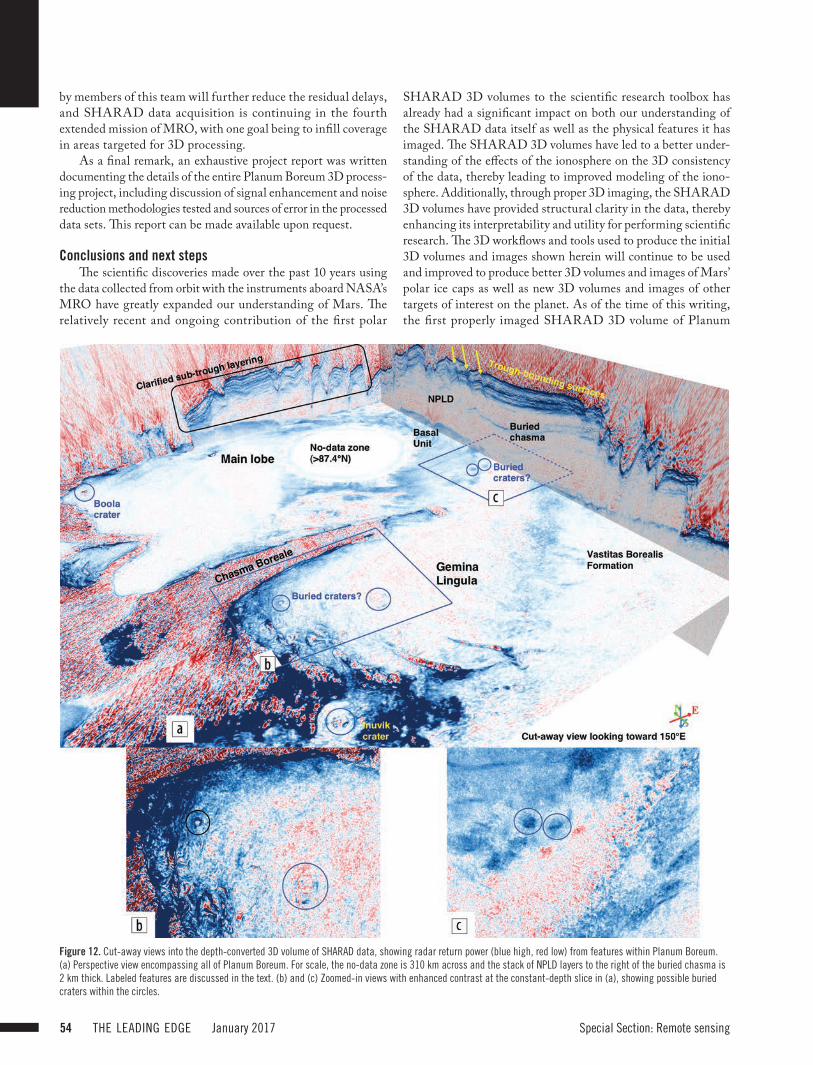
that were hidden by clutter or mispositioning in the 2D data set — such as structures in trough-dense regions (Smith et al., 2016; Figures 13 and 14) and what appear to be buried impact craters (Figure 12) — are newly revealed in the 3D volume. In particular, the 3D volume assisted (Smith et al., 2016) in fully mapping the extent of a shallow unconformity probably linked to a recent change in climate (see Introduction). Partially buried impact craters exhibit a distinctive signature that is repeated elsewhere in the volume but without surface expression. These features may be fully buried impact craters. For Earth’s moon, cratering statistics have been tied to radiometrically dated samples returned by the Apollo program, and the derived cratering rates have been extrapolated and used for dating surfaces on Mars and other bodies in the solar system. Thus, to the extent that a statistically significant number of the suspected buried craters can be demonstrated to be true impact craters, they will provide an important measure of the age of the icy layered deposits that is in-dependent of climate models.

Despite the discovery and removal of residual ionospheric time delays in the data, some residual time delays remain in the data that cannot be identified as variations in ionospheric phase distortion, as they are not correlated with solar zenith angle or the computed ionospheric phase distortion parameter modeled in the range compression step. These residual delay offsets re-maining in the data limited the effectiveness of 3D processing and reduced the vertical resolution by a factor of ~2 (Figure 14). Most notably, finer shallow layering and structures evident in the input 2D observations are not resolved in the 3D volume, hampering the ability (1) to improve upon prior efforts to correlate radar layering with that seen in visible imagery (e.g., Christian et al., 2013), (2) to map minor troughs and near-surface undula-tions linked to climate signals (e.g., Smith and Holt, 2015; Campbell et al., 2015), and (3) to visualize finer structures. In addition, coverage is still incomplete at the 475 m bin size, further limiting the resolution of finer features. A renewed effort

Figure 11. (a) Inline profile, (b) time slice, and (c) crossline profile through the Planum Australe SHARAD 3D volume after (piecewise) 3D downward continuation. Color indicates radar return reflection strength (blue high, red low). Thin red lines mark locations of adjacent views. Surface and subsurface features are resolved and no longer obscured by unfocused radar returns (“clutter”). In particular, a feature characterized by so-called “reflection free zones” (RFZs) separated by distinct bright reflectors located between the two dashed lines on the inline and time slice panels is clearly revealed after downward continuation (compare with Figure 10). Note that the faint “cross hatching” visible in the time slice is due to lingering truncation artifacts from the adjacent downward continued pieces (see text for additional discussion).


Figure 12. Cut-away views into the depth-converted 3D volume of SHARAD data, showing radar return power (blue high, red low) from features within Planum Boreum. (a) Perspective view encompassing all of Planum Boreum. For scale, the no-data zone is 310 km across and the stack of NPLD layers to the right of the buried chasma is 2 km thick. Labeled features are discussed in the text. (b) and (c) Zoomed-in views with enhanced contrast at the constant-depth slice in (a), showing possible buried craters within the circles.

SHARAD 3D volumes to the scientific research toolbox has already had a significant impact on both our understanding of the SHARAD data itself as well as the physical features it has imaged. The SHARAD 3D volumes have led to a better under-standing of the effects of the ionosphere on the 3D consistency of the data, thereby leading to improved modeling of the iono-sphere. Additionally, through proper 3D imaging, the SHARAD 3D volumes have provided structural clarity in the data, thereby enhancing its interpretability and utility for performing scientific research. The 3D workflows and tools used to produce the initial 3D volumes and images shown herein will continue to be used and improved to produce better 3D volumes and images of Mars’ polar ice caps as well as new 3D volumes and images of other targets of interest on the planet. As of the time of this writing, the first properly imaged SHARAD 3D volume of Planum

by members of this team will further reduce the residual delays, and SHARAD data acquisition is continuing in the fourth extended mission of MRO, with one goal being to infill coverage in areas targeted for 3D processing.

As a final remark, an exhaustive project report was written documenting the details of the entire Planum Boreum 3D process-ing project, including discussion of signal enhancement and noise reduction methodologies tested and sources of error in the processed data sets. This report can be made available upon request.

Conclusions and next stepsThe scientific discoveries made over the past 10 years using

the data collected from orbit with the instruments aboard NASA’s MRO have greatly expanded our understanding of Mars. The relatively recent and ongoing contribution of the first polar


Boreum has been completed, with the first such volume of Planum Australe almost complete and to be followed by other volumes imaging smaller targets at lower latitudes. Efforts are under way to archive the SHARAD 3D processing methodology and the resulting 3D data volumes in NASA’s Planetary Data System, thereby making them available to the broader scientific community. Additionally, because of the diagnostic power of 3D data analysis, there is an effort under way to detect and winnow out lingering ionospheric time delays and other timing inconsistencies between the individual radargrams that, if successful, will improve the resolution and thus interpretability of the SHARAD 3D volumes. Finally, through iterative sensitivity analysis and refinement of the 3D image provided by the SHARAD volumes, we hope to extract velocity and corresponding dielectric constant information for the

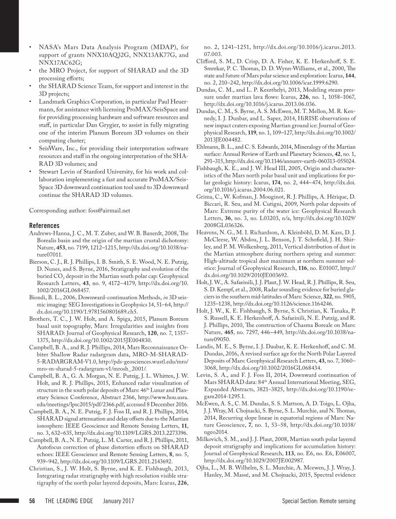
Figure 14. Detailed views of upper-left quadrants of panels in Figure 13 showing improvements to clutter interference and geometries afforded by the 3D processing. Segment where the surface is poorly sampled by MOLA laser altimetry data (‘MOLA “hole”’) is corrected in the 3D views using the SHARAD data itself.

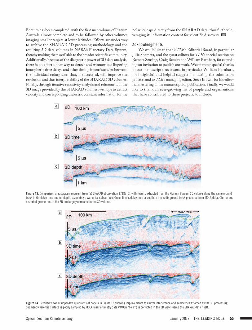
Figure 13. Comparison of radagram segment from (a) SHARAD observation 17187-01 with results extracted from the Planum Boreum 3D volume along the same ground track in (b) delay time and (c) depth, assuming a water-ice subsurface. Green line is delay time or depth to the nadir ground track predicted from MOLA data. Clutter and distorted geometries in the 2D are largely corrected in the 3D volume.

polar ice caps directly from the SHARAD data, thus further le-veraging its information content for scientific discovery.

AcknowledgmentsWe would like to thank TLE ’s Editorial Board, in particular

Julie Shemeta, and the guest editors for TLE ’s special section on Remote Sensing, Craig Beasley and William Barnhart, for extend-ing an invitation to publish our work. We offer our special thanks to our manuscript’s reviewers, in particular William Barnhart, for insightful and helpful suggestions during the submission process, and to TLE ’s managing editor, Steve Brown, for his edito-rial mastering of the manuscript for publication. Finally, we would like to thank an ever-growing list of people and organizations that have contributed to these projects, to include:


• NASA’s Mars Data Analysis Program (MDAP), for support of grants NNX10AQ32G, NNX13AK77G, and NNX17AC62G;

• the MRO Project, for support of SHARAD and the 3D processing efforts;

• the SHARAD Science Team, for support and interest in the 3D projects;

• Landmark Graphics Corporation, in particular Paul Heuer-mann, for assistance with licensing ProMAX/SeisSpace and for providing processing hardware and software resources and staff, in particular Dan Grygier, to assist in fully migrating one of the interim Planum Boreum 3D volumes on their computing cluster;

• SeisWare, Inc., for providing their interpretation software resources and staff in the ongoing interpretation of the SHA-RAD 3D volumes; and

• Stewart Levin of Stanford University, for his work and col-laboration implementing a fast and accurate ProMAX/Seis-Space 3D downward continuation tool used to 3D downward continue the SHARAD 3D volumes.

Corresponding author: [email protected]

ReferencesAndrews-Hanna, J. C., M. T. Zuber, and W. B. Banerdt, 2008, The

Borealis basin and the origin of the martian crustal dichotomy: Nature, 453, no. 7199, 1212–1215, http://dx.doi.org/10.1038/na-ture07011.

Bierson, C. J., R. J. Phillips, I. B. Smith, S. E. Wood, N. E. Putzig, D. Nunes, and S. Byrne, 2016, Stratigraphy and evolution of the buried CO2 deposit in the Martian south polar cap: Geophysical Research Letters, 43, no. 9, 4172–4179, http://dx.doi.org/10. 1002/2016GL068457.

Biondi, B. L., 2006, Downward-continuation Methods, in 3D seis-mic imaging: SEG Investigations in Geophysics 14, 51–64, http://dx.doi.org/10.1190/1.9781560801689.ch5.

Brothers, T. C., J. W. Holt, and A. Spiga, 2015, Planum Boreum basal unit topography, Mars: Irregularities and insights from SHARAD: Journal of Geophysical Research, 120, no. 7, 1357–1375, http://dx.doi.org/10.1002/2015JE004830.

Campbell, B. A., and R. J. Phillips, 2014, Mars Reconnaissance Or-biter Shallow Radar radargram data, MRO-M-SHARAD-5-RADARGRAM-V1.0, http://pds-geosciences.wustl.edu/mro/mro-m-sharad-5-radargram-v1/mrosh_2001/.

Campbell, B. A., G. A. Morgan, N. E. Putzig, J. L. Whitten, J. W. Holt, and R. J. Phillips, 2015, Enhanced radar visualization of structure in the south polar deposits of Mars: 46th Lunar and Plan-etary Science Conference, Abstract 2366, http://www.hou.usra.edu/meetings/lpsc2015/pdf/2366.pdf, accessed 8 December 2016.

Campbell, B. A., N. E. Putzig, F. J. Foss II, and R. J. Phillips, 2014, SHARAD signal attenuation and delay offsets due to the Martian ionosphere: IEEE Geoscience and Remote Sensing Letters, 11, no. 3, 632–635, http://dx.doi.org/10.1109/LGRS.2013.2273396.

Campbell, B. A., N. E. Putzig, L. M. Carter, and R. J. Phillips, 2011, Autofocus correction of phase distortion effects on SHARAD echoes: IEEE Geoscience and Remote Sensing Letters, 8, no. 5, 939–942, http://dx.doi.org/10.1109/LGRS.2011.2143692.

Christian, S., J. W. Holt, S. Byrne, and K. E. Fishbaugh, 2013, Integrating radar stratigraphy with high resolution visible stra-tigraphy of the north polar layered deposits, Mars: Icarus, 226,

no. 2, 1241–1251, http://dx.doi.org/10.1016/j.icarus.2013. 07.003.

Clifford, S. M., D. Crisp, D. A. Fisher, K. E. Herkenhoff, S. E. Smrekar, P. C. Thomas, D. D. Wynn-Williams, et al., 2000, The state and future of Mars polar science and exploration: Icarus, 144, no. 2, 210–242, http://dx.doi.org/10.1006/icar.1999.6290.

Dundas, C. M., and L. P. Keszthelyi, 2013, Modeling steam pres-sure under martian lava flows: Icarus, 226, no. 1, 1058–1067, http://dx.doi.org/10.1016/j.icarus.2013.06.036.

Dundas, C. M., S. Byrne, A. S. McEwen, M. T. Mellon, M. R. Ken-nedy, I. J. Dunbar, and L. Saper, 2014, HiRISE observations of new impact craters exposing Martian ground ice: Journal of Geo-physical Research, 119, no. 1, 109–127, http://dx.doi.org/10.1002/ 2013JE004482.

Ehlmann, B. L., and C. S. Edwards, 2014, Mineralogy of the Martian surface: Annual Review of Earth and Planetary Sciences, 42, no. 1, 291–315, http://dx.doi.org/10.1146/annurev-earth-060313-055024.

Fishbaugh, K. E., and J. W. Head III, 2005, Origin and character-istics of the Mars north polar basal unit and implications for po-lar geologic history: Icarus, 174, no. 2, 444–474, http://dx.doi.org/10.1016/j.icarus.2004.06.021.

Grima, C., W. Kofman, J. Mouginot, R. J. Phillips, A. Hérique, D. Biccari, R. Seu, and M. Cutigni, 2009, North polar deposits of Mars: Extreme purity of the water ice: Geophysical Research Letters, 36, no. 3, no. L03203, n/a, http://dx.doi.org/10.1029/ 2008GL036326.

Heavens, N. G., M. I. Richardson, A. Kleinböhl, D. M. Kass, D. J. McCleese, W. Abdou, J. L. Benson, J. T. Schofield, J. H. Shir-ley, and P. M. Wolkenberg, 2011, Vertical distribution of dust in the Martian atmosphere during northern spring and summer: High-altitude tropical dust maximum at northern summer sol-stice: Journal of Geophysical Research, 116, no. E01007, http://dx.doi.org/10.1029/2010JE003692.

Holt, J. W., A. Safaeinili, J. J. Plaut, J. W. Head, R. J. Phillips, R. Seu, S. D. Kempf, et al., 2008, Radar sounding evidence for buried gla-ciers in the southern mid-latitudes of Mars: Science, 322, no. 5905, 1235–1238, http://dx.doi.org/10.1126/science.1164246.

Holt, J. W., K. E. Fishbaugh, S. Byrne, S. Christian, K. Tanaka, P. S. Russell, K. E. Herkenhoff, A. Safaeinili, N. E. Putzig, and R. J. Phillips, 2010, The construction of Chasma Boreale on Mars: Nature, 465, no. 7297, 446–449, http://dx.doi.org/10.1038/na-ture09050.

Landis, M. E., S. Byrne, I. J. Daubar, K. E. Herkenhoff, and C. M. Dundas, 2016, A revised surface age for the North Polar Layered Deposits of Mars: Geophysical Research Letters, 43, no. 7, 3060–3068, http://dx.doi.org/10.1002/2016GL068434.

Levin, S. A., and F. J. Foss II, 2014, Downward continuation of Mars SHARAD data: 84th Annual International Meeting, SEG, Expanded Abstracts, 3821–3825, http://dx.doi.org/10.1190/se-gam2014-1295.1.

McEwen, A. S., C. M. Dundas, S. S. Mattson, A. D. Toigo, L. Ojha, J. J. Wray, M. Chojnacki, S. Byrne, S. L. Murchie, and N. Thomas, 2014, Recurring slope lineae in equatorial regions of Mars: Na-ture Geoscience, 7, no. 1, 53–58, http://dx.doi.org/10.1038/ngeo2014.

Milkovich, S. M., and J. J. Plaut, 2008, Martian south polar layered deposit stratigraphy and implications for accumulation history: Journal of Geophysical Research, 113, no. E6, no. E6, E06007, http://dx.doi.org/10.1029/2007JE002987.

Ojha, L., M. B. Wilhelm, S. L. Murchie, A. Mcewen, J. J. Wray, J. Hanley, M. Massé, and M. Chojnacki, 2015, Spectral evidence


for hydrated salts in recurring slope lineae on Mars: Nature Geoscience, 8, no. 11, 829–832, http://dx.doi.org/10.1038/ngeo2546.

Phillips, R. J., M. T. Zuber, S. E. Smrekar, M. T. Mellon, J. W. Head, K. L. Tanaka, N. E. Putzig, et al., 2008, Mars north polar deposits: stratigraphy, age, and geody-namical response: Science, 320, no. 5880, 1182–1185, http://dx.doi.org/10.1126/sci-ence.1157546.

Phillips, R. J., B. J. Davis, K. L. Tanaka, S. Byrne, M. T. Mellon, N. E. Putzig, R. M. Haberle, et al., 2011, Massive CO₂ ice deposits sequestered in the south polar layered deposits of Mars: Science, 332, no. 6031, 838–841, http://dx.doi.org/10.1126/sci-ence.1203091.

Picardi, G., D. Biccari, R. Seu, J. Plaut, W. T. K. Johnson, R. L. Jordan, A. Safaeinili, et al., 2004, MARSIS: Mars advanced radar for subsurface and ionosphere sound-ing, in Mars express: A European mission to the red planet, European Space Agency Special Publication: ESA SP, 1240, 51–69.

Plaut, J. J., 2005, An inventory of impact craters on the Martian south polar layered de-posits: Presented at Lunar and Planetary Science XXXVI, Abstract 2319.

Plaut, J. J., A. Safaeinili, J. W. Holt, R. J. Phillips, J. W. Head III, R. Seu, N. E. Put-zig, and A. Frigeri, 2009, Radar evidence for ice in lobate debris aprons in the mid-northern latitudes of Mars: Geophysical Research Letters, 36, no. 2, no. L2203, n/a, http://dx.doi.org/10.1029/2008GL036379.

Putzig, N. E., R. J. Phillips, B. A. Campbell, J. W. Holt, J. J. Plaut, L. M. Carter, A. F. Egan, F. Bernardini, A. Safaeinili, and R. Seu, 2009, Subsurface structure of Planum Boreum from Mars Reconnaissance Orbiter shallow radar soundings: Ica-rus, 204, no. 2, 443–457, http://dx.doi.org/10.1016/j.icarus.2009.07.034.

Schultz, P. H., R. S. Harris, S. J. Clemett, K. L. Thomas-Keprta, and M. Zarate, 2015, Preserved flora and organics in impact melt breccia: Geology, 43, 635–638, http://dx.doi.org/10.1130/G35343.1.

Seu, R., R. J. Phillips, G. Alberti, D. Biccari, F. Bonaventura, M. Bortone, D. Calabrese, et al., 2007a, Accumulation and erosion of Mars’ south polar layered deposits: Science, 317, no. 5845, 1715–1718, http://dx.doi.org/10.1126/science.1144120.

Seu, R., R. J. Phillips, D. Biccari, R. Orosei, A. Masdea, G. Picardi, A. Safaeinili, et al., 2007b, SHARAD sounding radar on the Mars Reconnaissance Orbiter: Journal of Geophysical Research, 112, no. E5, no. E05505, 1–18, http://dx.doi.org/10.1029/2006JE002745.

Smith, D. E., M. T. Zuber, H. V. Frey, J. B. Garvin, J. W. Head, D. O. Muhleman, G. H. Pettengill, et al., 2001, Orbiter laser altimeter: Experiment summary after the first year of global mapping of Mars: Journal of Geophysical Research, 106, no. E10, no. E10, 23689–23722, http://dx.doi.org/10.1029/2000JE001364.

Smith, I. B., and J. W. Holt, 2010, Onset and migration of spiral troughs on Mars re-vealed by orbital radar: Nature, 465, no. 7297, 450–453, http://dx.doi.org/10.1038/nature09049.

Smith, I. B., and J. W. Holt, 2015, Spiral trough diversity on the north pole of Mars, as seen by Shallow Radar (SHARAD): Journal of Geophysical Research, 120, no. 3, 362–387, http://dx.doi.org/10.1002/2014JE004720.

Smith, I. B., N. E. Putzig, R. J. Phillips, and J. W. Holt, 2016, A record of Martian ice ages: Science, 352, no. 6289, 1075–1078, http://dx.doi.org/10.1126/science.aad6968.

Stolt, R. H., 1978, Migration by Fourier transform: Geophysics, 43, no. 1, 23–48, http://dx.doi.org/10.1190/1.1440826.

Tanaka, K. L., J. A. P. Rodriguez, J. A. Skinner Jr., M. C. Bourke, C. M. Fortezzo, K. E. Herkenhoff, E. J. Kolb, and C. H. Okubo, 2008, North polar region of Mars: Ad-vances in stratigraphy, structure, and erosional modification: Icarus, 196, no. 2, 318–358, http://dx.doi.org/10.1016/j.icarus.2008.01.021.

Taner, M. T., F. Koehler, and R. E. Sheriff, 1979, Complex seismic trace analysis: Geo-physics, 44, no. 6, 1041–1063, http://dx.doi.org/10.1190/1.1440994.

Wray, J. J., S. T. Hansen, J. Dufek, G. A. Swayze, S. L. Murchie, F. P. Seelos, J. R. Skok, R. P. Irwin III, and M. S. Ghiorso, 2013, Prolonged magmatic activity on Mars in-ferred from the detection of felsic rocks: Nature Geoscience, 6, no. 12, 1013–1017, http://dx.doi.org/10.1038/ngeo1994.

Zurek, R. W., and S. E. Smrekar, 2007, An overview of the Mars Reconnaissance Or-biter (MRO) science mission: Journal of Geophysical Research, 112, no. E05S01, 1–22, http://dx.doi.org/10.1029/2006JE002701.

All sensors Processing 3D modelling 3D inversion Visualisation Analysis Utilities

Minerals Petroleum Near Surface Government Contracting Consulting Education

ModelVision Magnetic & Gravity

Interpretation System

with 30 years of applied research

www.tensor-research.com.au

Tel:

Documents

3D imaging of Mars’ polar ice caps using orbital radar data imaging of Mars’ polar ice caps using orbital radar data ... to date is NASA’s Mars Reconnaissance Orbiter (MRO) mission,