3D FFT with 2D decomposition

Roland Schulz

04/27/08

Abstract

Many scientific applications including molecular dynamics (MD)require a fast fourier transform (FFT). As the number of processorsfor high performance computer increases this transform has to be par-allelized to larger number of processors to remove it as a bottleneckfor the parallelization. This requires the decomposition to be changedfrom 1D to 2D. Such a 2D decomposed 3D FFT was implemented asthis project. With the 2D decomposition the limiting factor becomesthe required global transpose. This transpose can be speeded up byusing FFTW transpose instead of the standard MPI MPI_Alltoall.Having this 2D decomposed 3D FFTW allows to improve the scalingof the fastest available MD software.

1 Introduction

Fast fourier transform (FFT) is used for many scientific applications. Tobe able to show its importance and my interest in it I explain its usage inthe application I am most interested in which is molecular dynamics (MD)simulations. Because this requires some introduction into MD it is little bitlonger and can be skipped if only the FFT itself is of interest to the reader.

MD simulations give unique insides into dynamical processes on the atomiclevel for biological macromolecules and non-biological materials, because thecombination of times and length scales are not accessible to experiments.Recently the importance of high performance MD was discussed in nature-news [1] and portrayed as a competition between Schulten’s NAMD andD.E. Shaw’s Desmond. But contrary to this article, depending on the usedcommunication library, the fastest or second fastest MD software is GRO-MACS [2, 3] about even with Desmond as shown in Fig. 1. Because Desmondis not publically available, GROMACS is by large margin the fastest avail-able MD software for systems of the size of this standard benchmark. MDis computational challenging because we would like to simulate systems con-taining several million atoms for up to one millisecond of simulation time.MD requires to compute the force on each atom for every time-step. A time-step length is limited to 2 to 5fs. Thus to reach the desired simulation timesthe compute time for each time-step is limited to a thenth millisecond. The

1

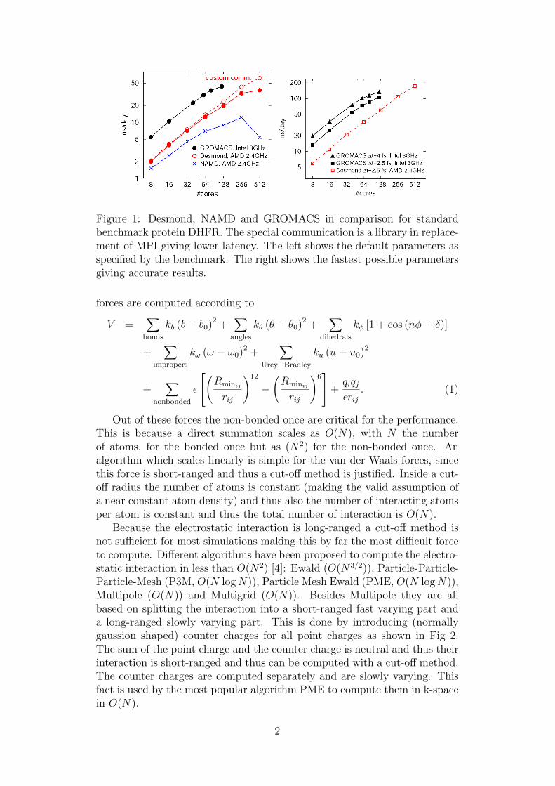
Figure 1: Desmond, NAMD and GROMACS in comparison for standardbenchmark protein DHFR. The special communication is a library in replace-ment of MPI giving lower latency. The left shows the default parameters asspecified by the benchmark. The right shows the fastest possible parametersgiving accurate results.

forces are computed according to

V =∑

bonds

kb (b− b0)2 +

∑

angles

kθ (θ − θ0)2 +

∑

dihedrals

kφ [1 + cos (nφ− δ)]

+∑

impropers

kω (ω − ω0)2 +

∑

Urey−Bradley

ku (u− u0)2

+∑

nonbonded

ε

(Rminij

rij

)12

−(

Rminij

rij

)6 +

qiqj

εrij

. (1)

Out of these forces the non-bonded once are critical for the performance.This is because a direct summation scales as O(N), with N the numberof atoms, for the bonded once but as (N2) for the non-bonded once. Analgorithm which scales linearly is simple for the van der Waals forces, sincethis force is short-ranged and thus a cut-off method is justified. Inside a cut-off radius the number of atoms is constant (making the valid assumption ofa near constant atom density) and thus also the number of interacting atomsper atom is constant and thus the total number of interaction is O(N).

Because the electrostatic interaction is long-ranged a cut-off method isnot sufficient for most simulations making this by far the most difficult forceto compute. Different algorithms have been proposed to compute the electro-static interaction in less than O(N2) [4]: Ewald (O(N3/2)), Particle-Particle-Particle-Mesh (P3M, O(N log N)), Particle Mesh Ewald (PME, O(N log N)),Multipole (O(N)) and Multigrid (O(N)). Besides Multipole they are allbased on splitting the interaction into a short-ranged fast varying part anda long-ranged slowly varying part. This is done by introducing (normallygaussion shaped) counter charges for all point charges as shown in Fig 2.The sum of the point charge and the counter charge is neutral and thus theirinteraction is short-ranged and thus can be computed with a cut-off method.The counter charges are computed separately and are slowly varying. Thisfact is used by the most popular algorithm PME to compute them in k-spacein O(N).

2

Figure 2: Counter charges used for long range electrostatic methods

Data can be transformed into from the k-space using the three dimen-sional fourier transform. It has been discovered several times independentfrom each other (most popular Cooley and Turkey 1965, first Gauss around1805) that this can be done by a divide and conquer algorithm in O(N log N).Thus also the full PME scales as O(N log N).

The discrete fourier transformation can be written as [5]

Xk =N−1∑

n=0

xne−2πiN

nk (2)

where Xk are the transformed values, xn are the input values and N are thenumber of input values. By splitting the sum into two parts with the oddand even ones, one gets the recursion formula:

Xk =

N2−1∑

m=0

x2me−2πiN

(2m)k +

N2−1∑

m=0

x2m+1e− 2πi

N(2m+1)k (3)

=M−1∑

m=0

x2me−2πiM

mk + e−2πiN

kM−1∑

m=0

x2m+1e− 2πi

Mmk (4)

=

{Ek + e−

2πiN

kOk if k < M

Ek−M − e−2πiN

(k−M)Ok−M if k ≥ M(5)

with M = N/2. Because Ok (and Ek) can be computed as Xk with theodd (respectively even) part of the input values this formula can be appliedrecursively until only two numbers are left. Formulas with other radix then2 also exists. This formula can be easily extended from this one dimensionalcase to the n-dimensional case by applying the 1D formula in turn onto eachdimension of the input data. A special case is real data which is very oftenthe input including for PME. The result is complex but because half of theresult is identical to the other half only half as much data has to be computedand stored as for complex input data. Complex data with this symmetry canin turn be back transformed to real data again in half as much CPU time.

”Fastest Fourier Transform in the West” (FFTW) [6] is a very fast im-plementation of one and multidimensional FFT, of arbitrary size, with real

3

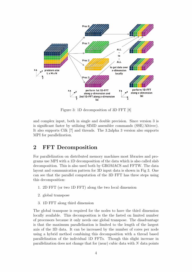
Figure 3: 1D decomposition of 3D FFT [8]

and complex input, both in single and double precision. Since version 3 isis significant faster by utilizing SIMD assembler commands (SSE/Altivec).It also supports Cilk [7] and threads. The 3.2alpha 3 version also supportsMPI for parallelization.

2 FFT Decomposition

For parallelization on distributed memory machines most libraries and pro-grams use MPI with a 1D decomposition of the data which is also called slabdecomposition. This is also used both by GROMACS and FFTW. The datalayout and communication pattern for 3D input data is shown in Fig 3. Onecan see that the parallel computation of the 3D FFT has three steps usingthis decomposition:

1. 2D FFT (or two 1D FFT) along the two local dimension

2. global transpose

3. 1D FFT along third dimension

The global transpose is required for the nodes to have the third dimensionlocally available. This decomposition is the the fasted on limited numberof processors because it only needs one global transpose. The disadvantageis that the maximum parallelization is limited to the length of the largestaxis of the 3D data. It can be increased by the number of cores per nodeusing a hybrid method combining this decomposition with a thread basedparallelization of the individual 1D FFTs. Though this slight increase inparallelization does not change that for (near) cubic data with N data points

4

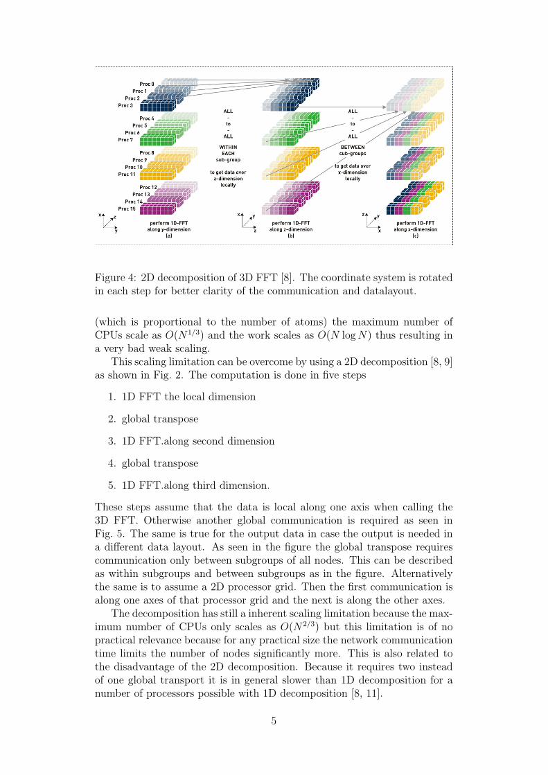
Figure 4: 2D decomposition of 3D FFT [8]. The coordinate system is rotatedin each step for better clarity of the communication and datalayout.

(which is proportional to the number of atoms) the maximum number ofCPUs scale as O(N1/3) and the work scales as O(N log N) thus resulting ina very bad weak scaling.

This scaling limitation can be overcome by using a 2D decomposition [8, 9]as shown in Fig. 2. The computation is done in five steps

1. 1D FFT the local dimension

2. global transpose

3. 1D FFT.along second dimension

4. global transpose

5. 1D FFT.along third dimension.

These steps assume that the data is local along one axis when calling the3D FFT. Otherwise another global communication is required as seen inFig. 5. The same is true for the output data in case the output is needed ina different data layout. As seen in the figure the global transpose requirescommunication only between subgroups of all nodes. This can be describedas within subgroups and between subgroups as in the figure. Alternativelythe same is to assume a 2D processor grid. Then the first communication isalong one axes of that processor grid and the next is along the other axes.

The decomposition has still a inherent scaling limitation because the max-imum number of CPUs only scales as O(N2/3) but this limitation is of nopractical relevance because for any practical size the network communicationtime limits the number of nodes significantly more. This is also related tothe disadvantage of the 2D decomposition. Because it requires two insteadof one global transport it is in general slower than 1D decomposition for anumber of processors possible with 1D decomposition [8, 11].

5

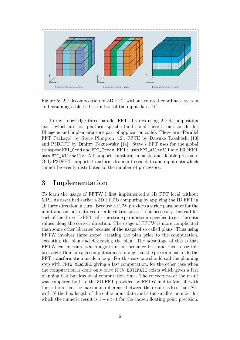
Figure 5: 2D decomposition of 3D FFT without rotated coordinate systemand assuming a block distribution of the input data [10]

To my knowledge three parallel FFT libraries using 2D decompositionexist, which are non platform specific (additional there is one specific forBluegene and implementations part of application code). These are “ParallelFFT Package” by Steve Plimpton [12], FFTE by Daisuke Takahashi [13]and P3DFFT by Dmitry Pekurovsky [14]. Steve’s FFT uses for the globaltranspose MPI_Send and MPI_Irecv, FFTE uses MPI_AlltoAll and P3DFFTuses MPI_Alltoallv. All support transform in single and double precision.Only P3DFFT supports transforms from or to real data and input data whichcannot be evenly distributed to the number of processors.

3 Implementation

To learn the usage of FFTW I first implemented a 3D FFT local withoutMPI. As described earlier a 3D FFT is computing by applying the 1D FFT inall three direction in turn. Because FFTW provides a stride parameter for theinput and output data vector a local transpose is not necessary. Instead foreach of the three 1D FFT calls the stride parameter is specified to get the datavalues along the correct direction. The usage of FFTW is more complicatedthan some other libraries because of the usage of so called plans. Thus usingFFTW involves three steps: creating the plan prior to the computation,executing the plan and destroying the plan. The advantage of this is thatFFTW can measure which algorithm performance best and then reuse thisbest algorithm for each computation assuming that the program has to do theFFT transformation inside a loop. For this case one should call the planningstep with FFTW_MEASURE giving a fast computation, for the other case whenthe computation is done only once FFTW_ESTIMATE exists which gives a fastplanning fast but less ideal computation time. The correctness of the resultwas compared both to the 3D FFT provided by FFTW and to Matlab withthe criteria that the maximum difference between the results is less than N3εwith N the box length of the cubic input data and ε the smallest number forwhich the numeric result is 1 + ε > 1 for the chosen floating point precision.

6

Since Matlab also internally uses FFTW this does not test the correctness ofFFTW but only the correctness of the usage of the library. Since FFTW isvery commonly used and has its built in tests, its correctness was assumed.

As a next step the 2D decomposition was implemented with MPI. Theglobal transpose is done with MPI_Alltoall and the 1D FFT by callingFFTW. I chose MPI_Alltoall for the global transpose because performancemeasurements on P3DFFT prior to the project showed that MPI_Alltoallvis significant slower than MPI_Alltoall and implementing an own fast globaltranspose based on MPI_Send and MPI_Recv is beyond the scope of theproject. I chose to use MPI_Alltoall without derived datatypes becauseI knew that they are not very efficient on the Cray MPI based on MPICH.

MPI_Alltoall without derived datatypes requires the data for each pro-cessor to be consecutive in memory. Additional the matrix transpose has dobe done locally after the submatrix are globally transposed by MPI_Alltoall.This local transpose could be avoided by using stride as was done in the localimplementation but because the memory has to be rearranged anyhow it isfaster to also do the local transpose so that FFTW can operate cache friendly.This also has the advantage to be able to measure this rearrangement timeindependent of the FFT time.

It is non trivial to implement this local memory rearrangement correctlybecause of the number of involved indices and the rotating coordinate system.Thus I implemented it in steps to reduce the initial complexity. The finalimplementation requires only that the input data is cubic and that the datacan be evenly distributed on the processor grid. It allows any size of cube ascomplex input both in single and double precision. The notation to describethe implemention steps is: N box length of data, P total number of processor,Px and Py are the number of processors along the sides of 2D processor grid,Nx = N/Px and Ny = N/Py. The steps are then:

1. each processor has only one input number, squared processor gridNx = Ny = 1

2. any size of data, squared processor gridPx = Py, Nx = Ny, Nx mod Px = 0

3. any size of data, any processor grid able to evenly divide dataNx mod Px = 0, Ny mod Py = 0

The first implementation did not require any local transpose and the secondimplementation had much simpler local transpose. The limitation of the finalimplementation to allow only evenly dividable data is caused by the choiceof MPI_Alltoall which does not allow to communicate different amountsof data per destination respectively source. The same reason applies to thelimitation to not allow transforms from or to real data but only complexto complex. The amount of data for real is (N + 1)/2. This means formost number of processor and input cube sizes the data will not be dividableevenly both for real and complex at the same time and thus the amountof data which would have to be communicated would vary. I started toimplement a version which also allows non cubic input data, but it complicate

7

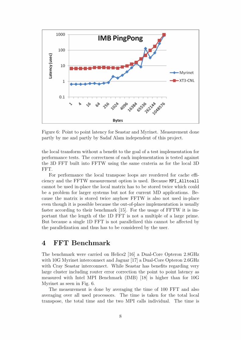
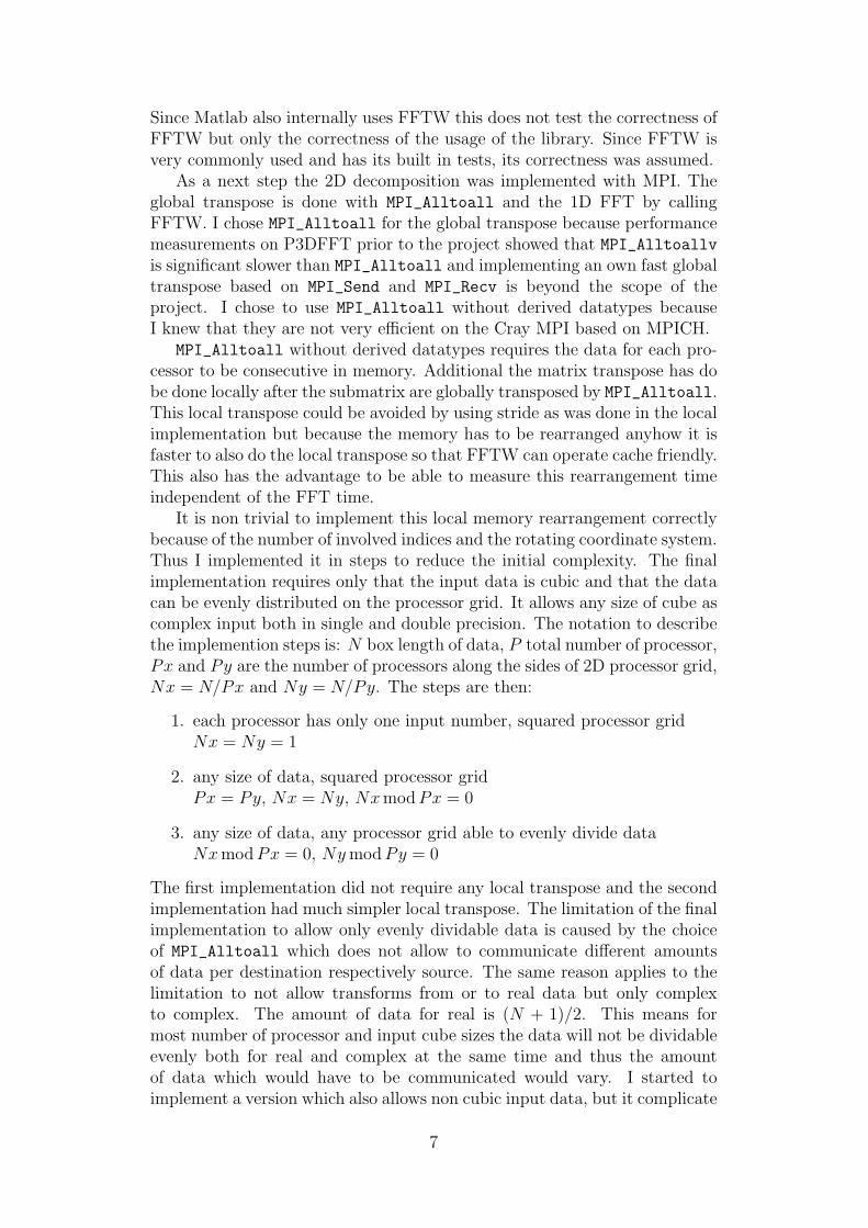
Figure 6: Point to point latency for Seastar and Myrinet. Measurement donepartly by me and partly by Sadaf Alam independent of this project.

the local transform without a benefit to the goal of a test implementation forperformance tests. The correctness of each implementation is tested againstthe 3D FFT built into FFTW using the same crateria as for the local 3DFFT.

For performance the local transpose loops are reordered for cache effi-ciency and the FFTW measurement option is used. Because MPI_Alltoall

cannot be used in-place the local matrix has to be stored twice which couldbe a problem for larger systems but not for current MD applications. Be-cause the matrix is stored twice anyhow FFTW is also not used in-placeeven though it is possible because the out-of-place implementation is usuallyfaster according to their benchmark [15]. For the usage of FFTW it is im-portant that the length of the 1D FFT is not a multiple of a large prime.But because a single 1D FFT is not parallelized this cannot be affected bythe parallelization and thus has to be considered by the user.

4 FFT Benchmark

The benchmark were carried on Helics2 [16] a Dual-Core Opteron 2.8GHzwith 10G Myrinet interconnect and Jaguar [17] a Dual-Core Opteron 2.6GHzwith Cray Seastar interconnect. While Seastar has benefits regarding verylarge cluster including router error correction the point to point latency asmeasured with Intel MPI Benchmark (IMB) [18] is higher than for 10GMyrinet as seen in Fig. 6.

The measurement is done by averaging the time of 100 FFT and alsoaveraging over all used processors. The time is taken for the total localtranspose, the total time and the two MPI calls individual. The time is

8

measure by MPI_Wtime. From measurement done prior to this project I knowthat 2D decomposition can be faster than 1D decomposition starting fromaround N = 128. Benchmarking my FFT implemented showed directly thatmost of the time is spent in the two MPI_Alltoall calls:

CPU Grid Local transpose FFT 1st MPI 2nd MPI2x64 0.30+/-0.01 0.66+/-0.01 122.93+/-87.64 3.24+/-26.724x32 0.25+/-0.01 0.65+/-0.01 59.01+/-42.27 4.04+/-25.748x16 0.25+/-0.01 0.65+/-0.01 92.38+/-26.07 8.94+/-33.2016x8 0.26+/-0.01 0.65+/-0.01 84.88+/-33.86 19.64+/-58.73

This data is for Helics2 but the conclusion is true also for Jaguar. The largestandard deviation originates from load implance. This can be seen by addinga MPI_Barrier before the first MPI_Wtime and after the second MPI_Wtime.This way timing of a task cannot be affected by the load imbalance fromthe task before. Of course one cannot add up the timings of the individualtask in this case because the effect of the load imbalance is not measuredaccurately anymore. The effect can be seen in the next measurement:

CPU Grid Local transpose FFT 1st MPI 2nd MPI16x8 0.25+/-0.00 0.65+/-0.01 4.18+/-13.03 75.93+/-60.12

The percentage of the MPI_Alltoall increases with larger number of pro-cessors because MPI_Alltoall decreases much slower than linearly. Becausemost time is spent in the global transpose I focused by benchmarking efforton this.

5 Global Transpose Benchmark

For the global transpose benchmark I used IMB both on Helics2 and Jaguar.I chose not to use my own code, so I wouldn’t have the overhead of the FFTand can clearly see the FFT by itself. Also IMB provides a nice matrix forthe timing in dependence both of message size and the number of processors,which is convenient not to have to write by oneself. For the MPI implemen-tation I used both the default implementation which is in both cases a vendormodified version of MPICH and the OpenMPI implementation with back-end for the highperformance interconnect. For Jaguar the version use werext-mpt/2.0.33 and openmpi/1.3a1r17992. On Helics2 I used MPICH-MX1.2.7..5 and OpenMPI 1.2.5.

By searching on the Internet for advice on global transpose I found the“FFTW MPI Transposes” [19] in FFTW 3.2alpha3. It is more general thanthe standard MPI_Alltoall but can be used as a compatible replacementfor MPI_Alltoall. It is not as general as MPI_Alltoallv but does supportdifferent message sizes per processor. It has three builtin implementation forthe communication. One is using direct point-to-point communication withprecomputed ordering to reduce the number of collisions. The second is usinga recursive ”radix-r” approach to reduce the number of messages to O(p log p)for p processors. The third implementation calls directly MPI_Alltoall orMPI_Alltoallv depending on whether the data is evenly dividable.

I had not seen this transpose in the FFTW documentation before becauseI mainly used the released version and did not look at the details of their

9

MPI implementation because it only uses slab decomposition. I added animplementation to IMB calling the FFTW MPI Transpose. As for the FFT,FFTW uses a planning phase to measure the fastest possible communicationpattern out of the three mentioned implementations. The timing is withoutthe planning phase assuming that it neglectable for long runs because it onlyhas to be executed once.

I used the normal scheduler and did not request a special reservationfor the benchmark. Thus the processors were in most cases not contiguousassigned. Heike Jagode has shown that on BlueGene the precise placing onthe 3D torus is very important [8]. Because Jaguar also uses a 3D torusis could potentially also be very important, even though according to JohnLevesque in a personal communication this effect should be small on Jaguar.Since I did not want to request a special reservation for this project I couldnot test it. Helics2 has a full-bisection diameter-3 Clos network and thus Ido not expect large effect on the placing. Again I did not request a specialreservation to test assumption.

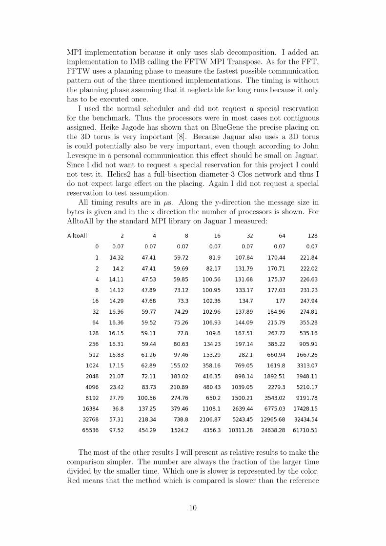
All timing results are in µs. Along the y-direction the message size inbytes is given and in the x direction the number of processors is shown. ForAlltoAll by the standard MPI library on Jaguar I measured:

The most of the other results I will present as relative results to make thecomparison simpler. The number are always the fraction of the larger timedivided by the smaller time. Which one is slower is represented by the color.Red means that the method which is compared is slower than the reference

10

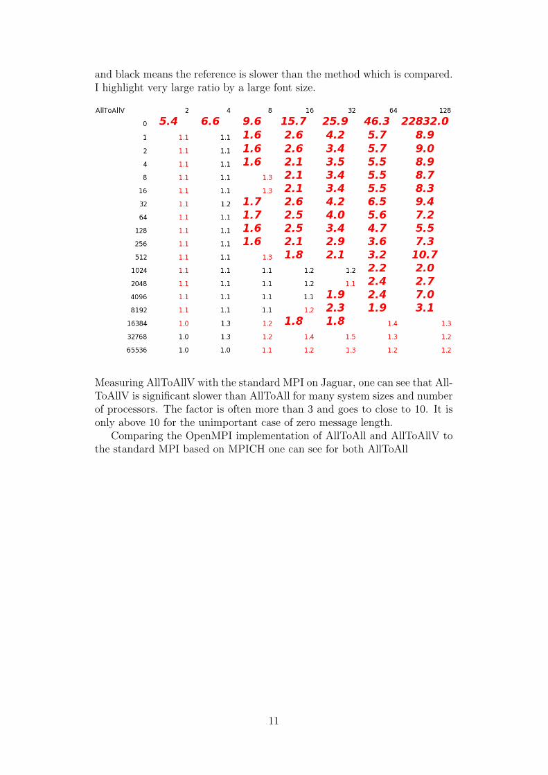
and black means the reference is slower than the method which is compared.I highlight very large ratio by a large font size.

Measuring AllToAllV with the standard MPI on Jaguar, one can see that All-ToAllV is significant slower than AllToAll for many system sizes and numberof processors. The factor is often more than 3 and goes to close to 10. It isonly above 10 for the unimportant case of zero message length.

Comparing the OpenMPI implementation of AllToAll and AllToAllV tothe standard MPI based on MPICH one can see for both AllToAll

11

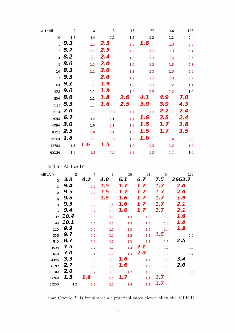
and for AllToAllV

that OpenMPI is for almost all practical cases slower than the MPICH

12

based MPI. The only expectation for practical cases and significant differenceis for some message sizes for 128 processors.

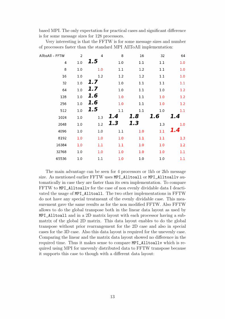
Very interesting is that the FFTW is for some message sizes and numberof processors faster than the standard MPI AllToAll implementation:

The main advantage can be seen for 4 processors or 1kb or 2kb messagesize. As mentioned earlier FFTW uses MPI_Alltoall or MPI_Alltoallv au-tomatically in case they are faster than its own implementation. To compareFFTW to MPI_Alltoallv for the case of non evenly dividable data I deacti-vated the usage of MPI_Alltoall. The two other implementations in FFTWdo not have any special treatmeant of the evenly dividable case. This mea-surement gave the same results as for the non modified FFTW. Also FFTWallows to do the global transpose both in the linear data layout as used byMPI_Alltoall and in a 2D matrix layout with each processor having a sub-matrix of the global 2D matrix. This data layout enables to do the globaltranspose without prior rearrangement for the 2D case and also in specialcases for the 3D case. Also this data layout is required for the unevenly case.Comparing the linear and the matrix data layout showed no difference in therequired time. Thus it makes sense to compare MPI_Alltoallv which is re-quired using MPI for unevenly distributed data to FFTW transpose becauseit supports this case to though with a different data layout:

13

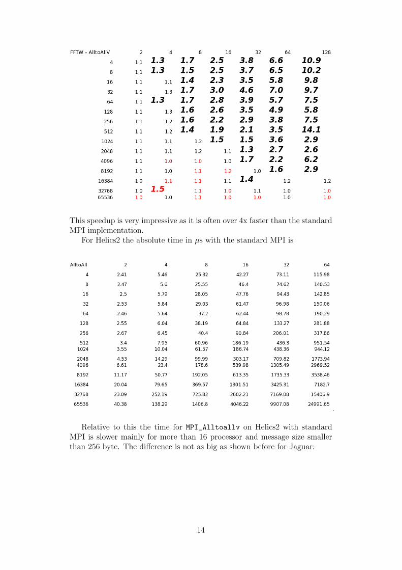
This speedup is very impressive as it is often over 4x faster than the standardMPI implementation.

For Helics2 the absolute time in µs with the standard MPI is

.

Relative to this the time for MPI_Alltoallv on Helics2 with standardMPI is slower mainly for more than 16 processor and message size smallerthan 256 byte. The difference is not as big as shown before for Jaguar:

14

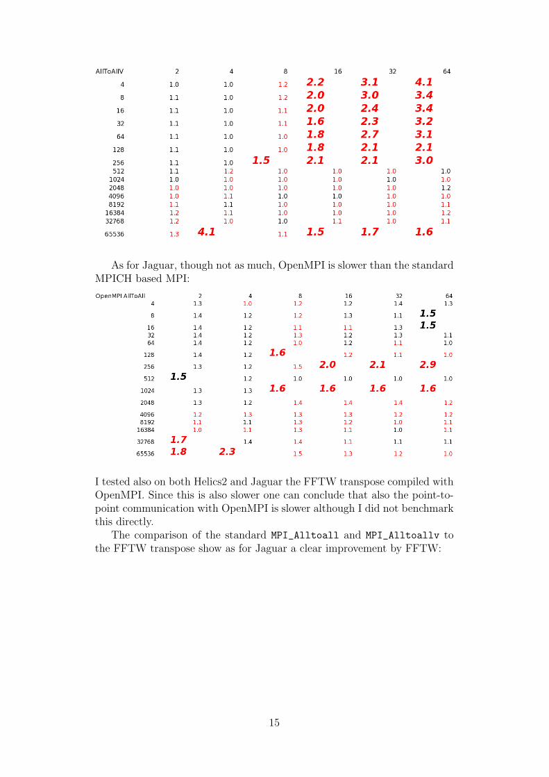
As for Jaguar, though not as much, OpenMPI is slower than the standardMPICH based MPI:

I tested also on both Helics2 and Jaguar the FFTW transpose compiled withOpenMPI. Since this is also slower one can conclude that also the point-to-point communication with OpenMPI is slower although I did not benchmarkthis directly.

The comparison of the standard MPI_Alltoall and MPI_Alltoallv tothe FFTW transpose show as for Jaguar a clear improvement by FFTW:

15

Eventhough one usually cannot choose the hardware to improve the li-brary performance, I think it is non the less interesting to compare Seastarto Myri 10G. Relative to Seastar Myri 10G is faster by:

16

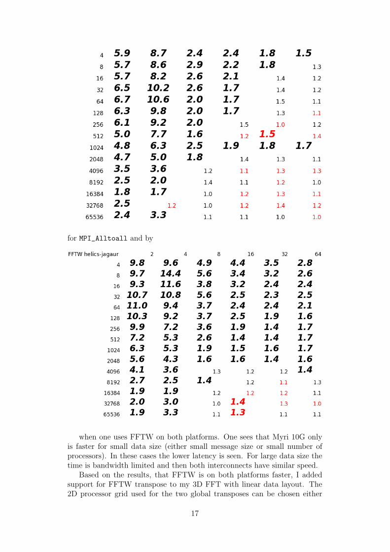
for MPI_Alltoall and by

when one uses FFTW on both platforms. One sees that Myri 10G onlyis faster for small data size (either small message size or small number ofprocessors). In these cases the lower latency is seen. For large data size thetime is bandwidth limited and then both interconnects have similar speed.

Based on the results, that FFTW is on both platforms faster, I addedsupport for FFTW transpose to my 3D FFT with linear data layout. The2D processor grid used for the two global transposes can be chosen either

17

(almost) square or very rectangular. Thus in the two global transpose thenumber of processors communicating to eachother is equal to the size of thegrid in this direction. The message size is for both communication the same.From the transpose results one can see that the time is increasing fasterthan linearly with the number of processors thus it is better to use a veryrectangular processor grid unless the application using the 3D FFT requiresa square processor grid. Thus I did not add a planning phase, as used byFFTW, to my 3D FFT because no parameter has to be optimized.

6 Possible further steps

It is also possible to use the matrix data layout for 3D matrices becauseFFTW transpose has a parameter “howmany” to specify blocks of data whichare kept consecutive during the transpose. Since this can only be appliedto consecutive data it applies only to dimemsion 1 (number from slowestdimension) thus it can only be applied to a transpose of dimension 2 and 3.As can be seen in the diagrams showing the commincation pattern for the2D decomposed FFT these two dimensions are not transposed but insteaddimension 1 and 2 and 1 and 3 are transposed. Thus also the matrix datalayout requires a local data reordering. I was not able to implement this afterI got the results from the transpose benchmarking.

Having implemented this data reordering, the matrix data layout FFTWtranspose will allow unevenly distributed data without a performance penalty.This allows for any size of input data and also real to complex transforms.The reduced amount of data for the real data should according to the trans-pose measurements give an improvement of 30%. The usage of real data andFFTW transpose should make the library faster than all other libraries andmore general than all but P3DFFT.

7 Conclusion

I have implemented a correct 3D FFT which is not limited by the datadecomposition as is FFTW and the FFT implemented in GROMACS. Thelimiting factor is the global transpose which was optimized by using theFFTW transpose. The measurements have shown that this FFTW transposeis faster both on Seastar and Myri 10G interconnect. This enables to extendthis implementation also to not dividable input sizes and real to complextransforms.

References

[1] Brendan Borrell. Chemistry: Power play. Nature News, 2008.

[2] B. Hess, C. Kutzner, D. Vanderspoel, and E. Lindahl. Gromacs 4: Al-gorithms for highly efficient, load-balanced, and scalable molecular sim-ulation. J. Chem. Theory Comput., February 2008.

18

[3] Gromacs. http://www.gromacs.org, 2008.

[4] C. Sagui and T. A. Darden. Molecular dynamics simulations of biomole-cules: long-range electrostatic effects. Annu Rev Biophys Biomol Struct,28:155–179, 1999.

[5] http://en.wikipedia.org/wiki/Cooley-Tukey_FFT_algorithm.

[6] http://www.fftw.org.

[7] http://supertech.csail.mit.edu/cilk.

[8] Heike Jagode. Fourier transforms for the bluegene/l communicationnetwork. Master’s thesis, The University of Edinburgh, 2005.

[9] Maria Eleftheriou, Jose E. Moreira, Blake G. Fitch, and Robert S. Ger-main. A volumetric fft for bluegene/l. pages 194–203. 2003.

[10] M. Eleftheriou, B. G. Fitch, A. Rayshubskiy, T. J. C. Ward, and R. S.Germain. Scalable framework for 3d ffts on the blue gene/l super-computer: Implementation and early performance measurements. IBMJournal of Research and Development, 49, 2005.

[11] Dmitry Pekurovsky. personal communication, 2008.

[12] Steve Plimpton. http://www.sandia.gov/~sjplimp/docs/fft/README.html.

[13] Daisuke Takahashi. http://www.ffte.jp/.

[14] Dmitry Pekurovsky. http://www.sdsc.edu/us/resources/p3dfft.php.

[15] http://www.fftw.org/speed/opteron-2.2GHz-64bit/.

[16] http://helics.iwr.uni-heidelberg.de.

[17] http://www.nccs.gov/computing-resources/jaguar.

[18] http://www3.intel.com/cd/software/products/asmo-na/eng/219848.htm.

[19] http://www.fftw.org/fftw-3.2alpha3-doc/FFTW-MPI-Transposes.html.

19