Embed Size (px)
Citation preview
INSTITUT FÜRSTATIK UND DYNAMIKDER LUFT- UNDRAUMFAHRTKONSTRUKTIONEN
UNIVERSITÄT STUTTGART
H. Matthias Deuschle
Be
rich
ta
us
de
mIn
stitu
t
3D Failure Analysis ofUD Fibre Reinforced Composites:Puck’s Theory within FEA
57-2
010

3D Failure Analysis ofUD Fibre Reinforced Composites:
Puck’s Theory within FEA
A thesis accepted by the Faculty of Aerospace Engineering and Geodesyof the Universitat Stuttgart in partial fulfilment of the requirements
for the degree of Doctor of Engineering Sciences (Dr.-Ing.)
byDipl.-Ing. H. Matthias Deuschle
born in Karlsruhe
Main referee: Prof. Dr.-Ing. habil. Bernd-Helmut KroplinCo-referee: Prof. Dr. rer. nat. Siegfried SchmauderDate of defence: September 6, 2010
Institute of Statics and Dynamics of Aerospace StructuresUniversitat Stuttgart
2010
Herausgeber: Prof. Dr.-Ing. Bernd Kroplin
D93
ISBN 3-930683-99-7
Dieses Werk ist urheberrechtlich geschutzt. Die dadurch begrundeten Rechte, insbesondere die der Uber-setzung, des Nachdrucks, des Vortrags, der Entnahme von Abbildungen und Tabellen, der Funksendung,der Mikroverfilmung oder der Vervielfaltigung auf anderen Wegen und der Speicherung in Datenverar-beitungsanlagen, bleiben, auch bei nur auszugsweiser Verwertung, vorbehalten. Eine Vervielfaltigungdieses Werkes oder von Teilen dieses Werkes ist auch im Einzelfall nur in den Grenzen der gesetzlichenBestimmungen des Urheberrechtsgesetzes der Bundesrepublik Deutschland vom 9. September 1965 in derjeweils geltenden Fassung zulassig. Sie ist grundsatzlich vergutungspflichtig. Zuwiderhandlungen unter-liegen den Strafbestimmungen des Urheberrechtsgesetzes.
c⃝ Institut fur Statik und Dynamik der Luft- und Raumfahrtkonstruktionen,Universitat Stuttgart, Stuttgart, 2010
Dieser Bericht kann uber das Institut fur Statik und Dynamik der Luft- und Raumfahrtkonstruktio-nen, Universitat Stuttgart, Pfaffenwaldring 27, 70569 Stuttgart, Telefon: (0711) 6856-63612, Fax:(0711) 6856-63706, bezogen werden.
Preface
The present work is the achievement of my activity as a research associate with the Institutfur Statik und Dynamik der Luft- und Raumfahrtkonstruktionen (ISD) at the UniversitatStuttgart. The completion of this dissertation has been possible thanks to the support ofmany people I would like to acknowledge:
Neither the participation in the WWFE-II nor the present thesis could have been realisedwithout the continuous support of Professor Alfred Puck. The phase-wise daily coopera-tion has been of inestimable value for both, me personally and for the project. Thank youfor your tireless effort to promote, generously share and impartially discuss your ideas.Your intellectual and literal hospitality will be a shining example to me.
I am deeply indebted to Professor Bernd-H. Kroplin who created and preserved an at-mosphere of free thinking, mutual trust, independence and personal responsibility at hisinstitute. These values have turned out to be precious in times of an increasing economi-sation and schoolification of the academic landscape. I am extremely grateful for theopportunity to benefit from as well as to contribute to the character of his outstandinginstitute.
Special thanks to Gunther Lutz and the Institute of Plastics Processing at RWTH AachenUniversity who generously provided the opportunity to introduce myself to the ”Puckcommunity” in 2008. The daily backing of my ISD colleagues has however been just asimportant. I am particularly grateful to Dr. Thomas Wallmersperger and Manfred Hahnwho have repeatedly delved deeply into my numerical and fracture mechanical problems.Thanks to the colleagues who made the effort to influence my way of thinking and formedthe particular spirit of the ISD and to all undergraduate students who worked on relevantsubjects within their theses.
I wish to express particular gratitude to my parents for providing a loving and respectfulparental home. They have constantly striven to open new worlds of experience to me be-sides reliably funding my education. Eventually they have handed me over to my personalmaterials science consultant, my beloved wife who patiently takes excellent care of me inall aspects.
Stuttgart, September 2010
H. Matthias Deuschle

Abstract
Unidirectionally fibre reinforced composites (UD FRCs) are an aspiring material wherehigh strength, adjustable stiffness, extraordinary durability and low weight is required.Their layer-wise processing into laminates enables the realisation of complex geometrieswith locally strongly differing properties. The design concept of integral constructionmakes use of this feature and combines different tasks in just one component. The in-creasing proportion of integral components brings significant savings in terms of struc-tural weight and maintenance cost of the overall system. This development is currentlyopposed by an enormous experimental effort which comes along with the application ofFRCs. The dimensioning of FRC laminates in terms of stiffness and strength has onlyhesitantly been included into efficient, computer-aided design processes. For the three-dimensional prediction of failure and post-failure behaviour there is currently no failuretheory available, which would have been implemented into a powerful design tool likeFinite Element Analysis (FEA) up to application maturity.
With Puck’s fracture criteria for unidirectionally fibre reinforces polymer composites (UDFRPCs), however, there is a per se three-dimensional failure hypothesis, which has provenits capability in the case of plane states of stress and which is successfully applied withinthe according restrictions. The present work aims on the verification of this failure modelfor a general three-dimensional load case, its appropriate extension and the combinationwith the capabilities of a commercial FE software package. The result is an implementa-tion which covers the layer-wise failure of a lamina and the successive damage evolutionwithin the laminate. Together with the interlaminar damage analysis which is alreadycomprised in such software packages, a comprehensive prediction tool for the damageprocess in UD FRC composites is generated.
The present work contains problems and approaches which are related to the achievementof the above mentioned goal. Starting with the representation of the nonlinear consti-tutive behaviour of an isolated lamina there occur specific three-dimensional problems.For example the material bears much more shear load under hydrostatic pressure, thancomprised in the uniaxially determined experimental stress-strain relation. Such cases aretreated by the self-similar scaling of the experimental curves. Being a stress-based crite-rion Puck’s Theory requires the full spacial stress tensor, as soon as a three-dimensionalprediction is striven for. It is shown that only few of the commercially implemented fi-nite element formulations are capable of providing these results in the case of shell-like
viii
structures. The quality of the results is evaluated by means of the analytical solutionfollowing Pagano. Puck’s criteria for fibre and inter-fibre fracture (IFF) include someextensions which gain importance particularly in the three-dimensional stress case. Theinfluences of fibre-parallel stress on the inter-fibre fracture and vice versa are presentedin the present work and their fracture-mechanical basis is demonstrated. In particular theinfluence of stresses, which are not acting on the fracture plane, strongly increases in thethree-dimensional case. The versatility of Puck’s inter-fibre fracture criterion is provedby its adjustment to the application to isotropic and not intrinsically brittle materials. Re-garding the successive three-dimensional damage after the occurrence of an inter-fibrefracture the existing degradation methods have been identified as insufficient. A fractureangle-dependent approach is developed, which homogenises the effect of the fracturesand defines the impact on the several stiffnesses. Virtual material tests on representativelaminate sections which contain discrete cracks prove the applicability of the developedrelations. The described failure and post-failure degradation models are prepared for theapplication within an implicit Finite Element Analysis. Their implementation into thecommercial software package ABAQUS is modular whereas the post-processing of con-ventionally derived or existing stress fields is sufficient for a pure failure prediction. Onlyif the post-failure degradation process is to be analysed, deeper manipulations of the FEanalysis in form of a user-defined material subroutine are necessary. The applicabilityof the generated implementation is proved by the analysis of twelve test cases which areprovided by the second World Wide Failure Exercise (WWFE-II). The given test casescomprise the failure and post-failure analysis of pure matrix material, of isolated laminaeand of laminates subjected to three-dimensional load. All the test cases are treated withan identical subroutine, hence with a single, consistent failure theory and the results areinterpreted regarding the actual material behaviour and the underlying failure predictionapproaches. It is shown that the application of Puck’s fracture hypotheses within a Fi-nite Element Analysis is a versatile and efficient tool for the three-dimensional failureprediction in UD FRC laminates.
Zusammenfassung
Unidirektional faserverstarkte Verbundwerkstoffe sind uberall dort ein zukunftstrachtigesMaterial, wo hohe Festigkeit, variable Steifigkeit, außerordentliche Haltbarkeit und leich-tes Gewicht von Vorteil sind. Ihre schichtweise Verarbeitung zu Laminaten erlaubt es,komplexe Geometrien mit lokal stark unterschiedlichen Eigenschaften zu erzeugen. Daskonstruktive Konzept der Integralbauweise macht sich diese Fahigkeiten zunutze und ver-eint so mehrere Aufgaben in einem Bauteil. Der zunehmende Anteil an Integralbauteilenerlaubt bedeutende Einsparungen hinsichtlich Gewicht und Wartungskosten des Gesamt-systems. Dieser Entwicklung steht momentan ein hoher experimenteller Aufwand ent-gegen, der mit der Verwendung von Faserverbund-Laminaten einher geht. Die Ausle-gung von Faserverbund-Laminaten hinsichtlich Steifigkeit und Festigkeit hat erst zoger-lich Eingang in effiziente, computer-unterstutzte Entwurfsprozesse gefunden. Fur diedreidimensionale Vorhersage des Versagens- und Nachversagensverhalten steht momen-tan kein Versagensmodell bereit, das bis zur Anwendungsreife in ein leistungsfahigesAuslegungswerkzeug wie die Finite Elemente (FE) Analyse integriert ware.
Mit den Puck’schen Bruchkriterien fur unidirektional faserverstarkte Polymer-Verbundesteht jedoch eine per se dreidimensionale Versagenshypothese zur Verfugung, derenLeistungsfahigkeit fur den ebenen Spannungsfall bereits bewiesen wurde und mit denentsprechenden Einschrankungen erfolgreich eingesetzt wird. Die vorliegende Arbeitverfolgt das Ziel, dieses Versagensmodell fur den allgemeinen, dreidimensionalen Span-nungsfall zu ertuchtigen, gegebenenfalls zu erweitern und mit der Leistungsfahigkeiteiner kommerziellen FE-Software zu verbinden. Ergebnis ist eine Implementierung, diedas schichtweise Versagen eines Laminates und die fortschreitende Schadigung des Ver-bundes umfasst. Zusammen mit den interlaminaren Schadigungsmodellen, die bereitsin derartigen Softwarepaketen enthalten sind, ergibt sich so eine umfassende Vorher-sagemoglichkeit des Schadigungsprozesses in Faserverbund-Laminaten.
Die vorliegende Arbeit behandelt Probleme und Losungsansatze, die mit dem Er-reichen dieses Ziels verbunden sind. Bereits bei der Abbildung des nichtlinearen kon-stitutiven Verhaltens einer Einzelschicht treten spezifisch dreidimensionale Problemeauf. Beispielsweise ertragt der Werkstoff unter hydrostatischem Druck weit mehrSchubbeanspruchung, als die einachsig ermittelte Schubspannungs-Scherungskurve um-fasst. Solche Falle werden durch die selbstahnliche Skalierung der experimentellenKurven behandelt. Als spannngsbasiertes Kriterium benotigt Puck’s Theorie den kom-
x
pletten raumlichen Spannungstensor, sobald eine dreidimensionale Vorhersage getrof-fen werden soll. Es wird gezeigt, dass nur wenige der kommerziell implementiertenfiniten Elementformulierungen in der Lage sind, dieses Ergebnis fur schalenartige Struk-turen bereit zu stellen. Die Gute dieser Ergebnisse wird anhand der analytischenLosung nach Pagano beurteilt. Die Puck’schen Kriterien fur Faser- und Zwischen-faserbruch umfassen eine Reihe von Erweiterungen, die gerade im raumlichen Span-nungsfall an Relevanz gewinnen. Die Einflusse von faserparallelen Spannungen auf denZwischenfaserbruch und umgekehrt werden in dieser Arbeit dargelegt und ihr bruch-mechanischer Hintergrund beleuchtet. Insbesondere der Einfluss der Spannungen, dienicht auf der Bruchebene wirken, nimmt im dreidimensionalen Fall stark zu. Die Viel-seitigkeit des Puck’schen Zwischenfaserbruch-Kriteriums wird dadurch bewiesen, dasses an die Anwendung auf isotrope und nicht intrinsisch sprode Werkstoffe angepasstwird. Hinsichtlich der fortschreitenden dreidimensionalen Schadigung nach Eintreteneines Zwischenfaserbruches haben sich die vorhanden Degradationsmethoden als unzure-ichend erwiesen. Es wird ein bruchwinkelabhangiges Verfahren entwickelt, mit demdie Auswirkung der Schadigung homogenisiert und den entsprechenden Steifigkeitenzugeschlagen wird. Durch virtuelle Materialtests an Laminat-Ausschnitten, die diskreteRisse enthalten, wird die Anwendbarkeit der entwickelten Zusammenhange bestatigt. Diebeschriebenen Versagens- und Degradationsmodelle werden zur Anwendung innerhalbeiner impliziten FE Analyse aufbereitet. Ihre Implementierung in das kommerzielle Pro-grammpaket ABAQUS kann modular erfolgen, wobei fur die reine Versagensvorhersageein Postprocessing von konventionell erzeugten oder bereits vorhandenen Spannungs-feldern ausreicht. Erst wenn das Degradationsverhalten entsprechend abgebildet wer-den soll, werden tiefere Eingriffe in die FE-Analyse in Form einer benutzerdefiniertenMaterial-Subroutine notwendig. Die Anwendungstauglichkeit der entstandenen Imple-mentierung wird durch die Analyse von zwolf Testfallen bewiesen, die dem World WideFailure Exercise II entspringen. Die gegebenen Testfalle umfassen die Versagens- undNachversagensanalyse von reinem Matrixmaterial, von Einzelschichten und Laminatenunter raumlicher Beanspruchung. Alle Testfalle werden mit der selben Subroutine, dem-nach mit einem konsistenten Versagensmodell bearbeitet und die Ergebnisse werden hin-sichtlich des Materialverhaltens und modelltheoretisch interpretiert. Es wird gezeigt, dassdie Anwendung der Puck’schen Bruchhypothesen im Rahmen der Finite Elemente Meth-ode ein vielseitiges und effizientes Werkzeug zur dreidimensionalen Schadensvorhersagein Faserverbund-Laminaten darstellt.
Contents
1 Introduction 1
1.1 Motivation . . . . . . . . . . . . . . . . . . . . . . . . . . . . . . . . . . 1
1.2 Problems and aims . . . . . . . . . . . . . . . . . . . . . . . . . . . . . 2
1.3 Structure of the present work . . . . . . . . . . . . . . . . . . . . . . . . 3
2 Failure of UD fibre-reinforced composites 7
2.1 Scales and coordinate systems of the material . . . . . . . . . . . . . . . 72.1.1 Micro-mechanical level . . . . . . . . . . . . . . . . . . . . . . . 72.1.2 Lamina level . . . . . . . . . . . . . . . . . . . . . . . . . . . . 82.1.3 Laminate level . . . . . . . . . . . . . . . . . . . . . . . . . . . 82.1.4 Structural level . . . . . . . . . . . . . . . . . . . . . . . . . . . 9
2.2 Types of failure . . . . . . . . . . . . . . . . . . . . . . . . . . . . . . . 92.2.1 Micro-damage . . . . . . . . . . . . . . . . . . . . . . . . . . . 92.2.2 Fibre fracture . . . . . . . . . . . . . . . . . . . . . . . . . . . . 102.2.3 Inter-fibre fracture . . . . . . . . . . . . . . . . . . . . . . . . . 112.2.4 Delamination . . . . . . . . . . . . . . . . . . . . . . . . . . . . 12
2.3 Successive failure . . . . . . . . . . . . . . . . . . . . . . . . . . . . . . 122.3.1 Damage evolution in a confined lamina . . . . . . . . . . . . . . 132.3.2 Successive failure of a laminate . . . . . . . . . . . . . . . . . . 14
2.4 Failure on the structural level . . . . . . . . . . . . . . . . . . . . . . . . 152.4.1 Torsion spring . . . . . . . . . . . . . . . . . . . . . . . . . . . 152.4.2 Integral vehicle rear suspension . . . . . . . . . . . . . . . . . . 162.4.3 Pressure vessel . . . . . . . . . . . . . . . . . . . . . . . . . . . 17
3 3D stress analysis in laminates and structures 19
3.1 Constitutive behaviour of a lamina . . . . . . . . . . . . . . . . . . . . . 193.1.1 Transverse isotropy and orthotropy . . . . . . . . . . . . . . . . 193.1.2 Nonlinearities in the constitutive behaviour . . . . . . . . . . . . 21
xii CONTENTS
3.1.3 Interaction between transverse and shear deformation . . . . . . . 23
3.2 FE representation of laminates and laminate structures . . . . . . . . . . 25
3.2.1 Equivalent single layer approaches . . . . . . . . . . . . . . . . . 27
3.2.2 Layer-wise approach . . . . . . . . . . . . . . . . . . . . . . . . 28
3.3 Laminate and laminate structures in commercial FE codes . . . . . . . . 29
3.3.1 Material definitions for laminates . . . . . . . . . . . . . . . . . 29
3.3.2 Element types for laminate structures . . . . . . . . . . . . . . . 30
3.4 Reference: Analytical solution following Pagano . . . . . . . . . . . . . 33
3.5 Generalised laminate behaviour: FEA of an RVE . . . . . . . . . . . . . 38
3.6 Geometric nonlinearity . . . . . . . . . . . . . . . . . . . . . . . . . . . 41
3.6.1 Load application . . . . . . . . . . . . . . . . . . . . . . . . . . 42
3.6.2 Engineering vs. true stresses and strains . . . . . . . . . . . . . . 42
3.7 Residual stresses . . . . . . . . . . . . . . . . . . . . . . . . . . . . . . 44
4 Puck’s failure theory 45
4.1 Introduction to failure prediction . . . . . . . . . . . . . . . . . . . . . . 45
4.2 Puck’s inter-fibre fracture criterion . . . . . . . . . . . . . . . . . . . . . 47
4.2.1 Action plane-related fracture criterion . . . . . . . . . . . . . . . 47
4.2.2 Application-oriented aspects of Puck’s IFF criterion . . . . . . . 51
4.2.3 Visual and mathematical representation – the MFB . . . . . . . . 54
4.2.4 IFF fracture modes classification for 3D analysis . . . . . . . . . 58
4.3 Influences on the IFF beyond Mohr’s hypothesis . . . . . . . . . . . . . . 60
4.3.1 Influences of fibre-parallel stress 𝜎1 . . . . . . . . . . . . . . . . 60
4.3.2 Influence of non-fracture plane stresses . . . . . . . . . . . . . . 63
4.4 Puck’s IFF criteria and the Mohr’ circle . . . . . . . . . . . . . . . . . . 68
4.5 Confined laminae – the In-Situ Effect . . . . . . . . . . . . . . . . . . . 71
4.6 Application of Puck’s IFF criterion to special cases . . . . . . . . . . . . 71
4.6.1 Application to isotropic material . . . . . . . . . . . . . . . . . . 71
4.6.2 Application to not intrinsically brittle materials . . . . . . . . . . 73
4.7 Puck’s fibre fracture criterion . . . . . . . . . . . . . . . . . . . . . . . . 74
xiii
5 Post-failure degradation analysis 77
5.1 Stability of the damage evolution in a laminate . . . . . . . . . . . . . . 77
5.2 Smeared crack representation . . . . . . . . . . . . . . . . . . . . . . . . 78
5.3 Existing degradation procedures . . . . . . . . . . . . . . . . . . . . . . 79
5.3.1 Excessive IFF stress exposure . . . . . . . . . . . . . . . . . . . 80
5.3.2 Constant IFF stress exposure . . . . . . . . . . . . . . . . . . . . 82
5.4 Variable IFF stress exposure . . . . . . . . . . . . . . . . . . . . . . . . 84
5.5 3D degradation procedure . . . . . . . . . . . . . . . . . . . . . . . . . . 84
5.6 RVE-studies on a discrete cracks . . . . . . . . . . . . . . . . . . . . . . 88
5.6.1 Derivation of the equivalent stiffness of a damaging lamina . . . . 90
5.6.2 Results of the RVE virtual material tests . . . . . . . . . . . . . . 92
5.7 Application-oriented summary . . . . . . . . . . . . . . . . . . . . . . . 98
6 Implementation of Puck’s Theory in ABAQUS 99
6.1 Implicit and explicit FEA . . . . . . . . . . . . . . . . . . . . . . . . . . 99
6.2 User-defined material behaviour subroutine . . . . . . . . . . . . . . . . 101
7 World Wide Failure Exercise II 105
7.1 Degradation aspects of the WWFE-II . . . . . . . . . . . . . . . . . . . . 105
7.2 Results of the WWFE-II test cases . . . . . . . . . . . . . . . . . . . . . 106
7.2.1 Homogeneous isotropic matrix test case . . . . . . . . . . . . . . 108
7.2.2 Lamina test cases . . . . . . . . . . . . . . . . . . . . . . . . . . 109
7.2.3 Laminate test cases . . . . . . . . . . . . . . . . . . . . . . . . . 115
8 Conclusion and Outlook 121
Appendix 127
A Derivation of the Pagano analytical solution . . . . . . . . . . . . . . . . 127
B WWFE-II test cases . . . . . . . . . . . . . . . . . . . . . . . . . . . . . 132
B.1 Given Instructions . . . . . . . . . . . . . . . . . . . . . . . . . 132
B.2 Given material parameters . . . . . . . . . . . . . . . . . . . . . 134

xiv CONTENTS
B.3 Given load cases . . . . . . . . . . . . . . . . . . . . . . . . . . 136
C Material data of HexPly 8551-7 (IM7) . . . . . . . . . . . . . . . . . . . 137
Bibliography 148
Notation
Coordinate Systems
𝑥, 𝑦, 𝑧 Global coordinate system of a laminate𝑥1, 𝑥2, 𝑥3 Coordinate system of a UD lamina, 𝑥1 being fibre-parallel,
𝑥3 in through-thickness direction𝑥∥, 𝑥⊥ Cylindrical coordinate system of a UD lamina, 𝑥∥ being fibre-parallel𝑥1, 𝑥𝑛, 𝑥𝑡 Coordinate system of an action plane, 𝑥1 being fibre-parallel
Arabic characters
𝑐 Index denoting compression𝐸 Stiffness matrix𝑓 Index denoting fibres’ figures𝑓𝐸 Stress exposure𝑓𝑆 Stretch factor𝑓𝑟, 𝑓𝑝 Index denoting fracture / fracture plane𝐹𝐹, 𝐼𝐹𝐹 Index denoting figures concerning fibre fracture / inter-fibre fracture𝑚 Minimum of the weakening factor 𝜂𝑤1𝑚𝜎𝑓 Magnification factor for matrix stresses𝑘 Shear impact degradation measure𝑙 Stress exposure impact degradation measure𝑛 Orientation impact degradation measure𝑝 Inclination parameter𝑅 Strength of the material𝑅𝐴 Fracture resistance of the action plane𝑠 Threshold of the 𝜂𝑤1 influence𝑆 Integrated standardised stress exposure𝑆 Compliance matrix𝑡 Index denoting tension
xvi CONTENTS
Greek characters
𝛼 Thermal expansion coefficient𝛽 Orientation of a lamina within an laminate𝛾 Shear strain𝛿 Macroscopic crack density𝜖 Normal strain𝜂 Degradation progress measure𝜂𝑚+𝑝 Weakening factor due to micro-damage and probabilistics𝜂𝑤1 Weakening factor due to fibre-parallel stresses 𝜎1
𝜃 Orientation of an action plane𝜈 Poisson’s ratio𝜎 Normal stress𝜏 Shear stress𝜑 Second angle unambiguously defining an action plane in isotropic material𝜓 Direction of the resultant shear in an action plane
xvii
Abbreviations
2D two-dimensional3D three-dimensionalBMBF Bundesministerium fur Bildung und Forschung
Federal Ministry of Education and researchCAE computer aided designCFRC carbon fibre reinforced compositeCLT classical laminate theoryCPU central processing unitESL equivalent single layerFE finite elementFEA finite element analysisFF fibre fractureFRC fibre reinforced compositeFRPC fibre reinforced polymer compositeFSDT first-order shear deformation theoryGFRC glass fibre reinforced compositeGMC generalised method of cellsHSDT higher-order shear deformation theoryIFF inter-fibre fractureMFB Master Fracture BodyLW layer-wisePVD principle of virtual displacementRMVT Reissner’s mixed variational theoremRVE representative volume elementSFB Sonderforschungsbereich / collaborative research centreUD unidirectional / unidirectionallyUMAT user material behaviour subroutineWWFE World Wide Failure Exercise

1 Introduction
1.1 Motivation
Engineering composite materials have been present in research and industry for severaldecades. Starting in the 1950s designs have been realised which heavily rely on the mainfeatures of unidirectionally fibre-reinforced composite (UD FRC) laminates – the lowweight to strength ratio and the individually adjustable constitutive characteristics. Alongwith comprehensive experimental effort extraordinary durable designs of lightweight cov-erings and casings as well as first structurally integrated parts in sail-planes, wind turbinesand yachts have been realised. In the beginning the advantages of UD FRCs in terms ofstrength, weight, and manufacturing outbalanced the high necessary safety factors due tothe lack of predictability of the material’s behaviour. Nowadays, however, security fac-tors are opposed to commercial aspects and the material selection is stronger influencedby the expense and reliability of its behaviour prediction than by the material’s capabili-ties itself. In this context numerical predictions gain more and more importance in orderto omit expensive experiments.
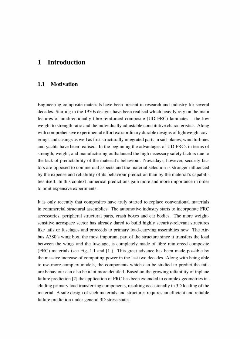
It is only recently that composites have truly started to replace conventional materialsin commercial structural assemblies. The automotive industry starts to incorporate FRCaccessories, peripheral structural parts, crash boxes and car bodies. The more weight-sensitive aerospace sector has already dared to build highly security-relevant structureslike tails or fuselages and proceeds to primary load-carrying assemblies now. The Air-bus A380’s wing box, the most important part of the structure since it transfers the loadbetween the wings and the fuselage, is completely made of fibre reinforced composite(FRC) materials (see Fig. 1.1 and [1]). This great advance has been made possible bythe massive increase of computing power in the last two decades. Along with being ableto use more complex models, the components which can be studied to predict the fail-ure behaviour can also be a lot more detailed. Based on the growing reliability of inplanefailure prediction [2] the application of FRC has been extended to complex geometries in-cluding primary load transferring components, resulting occasionally in 3D loading of thematerial. A safe design of such materials and structures requires an efficient and reliablefailure prediction under general 3D stress states.
2 CHAPTER 1. INTRODUCTION
Figure 1.1: The application of composite materials in the Airbus A380. (By courtesy ofAirbus)
1.2 Problems and aims
Within the collaborative research centre SFB-381 (1994-2006, [3]) the Univeritat Stuttgarthas generated significant knowledge on the Characterisation of Damage Development inComposite Materials Using Nondestructive Methods (SFB title). The project has iden-tified damage mechanisms on different lengths-scales and developed the experimentalapproaches to detect and monitor their occurrence, evolution and interaction. The re-vealed relations have been covered by appropriate mathematical descriptions and the as-sociated parameters have been determined for various material systems like wood, shortand long fibre reinforced polymer composites or steel reinforced concrete. The resultingtheories span from statistical descriptions of the successive fibre fracture (fibre bundlemodels), over the description of stress concentration fields around successively failingfibres up to macroscopic post-failure degradation models. The sub-project Numerical si-mulation of damage evolution included the implementation of the generated knowledgeinto application-oriented engineering tools. Aiming on the convenient application withina generally three-dimensional stress analysis, the Institute of Statics and Dynamics ofAerospace Structures (ISD) has evaluated several failure prediction approaches for UDFRPCs. The main requirements were a fracture mechanical basis and an open, accessiblestructure which allows the incorporation of various actual and future aspects.
Puck’s action plane-related failure criteria for unidirectional (UD) fibre reinforced poly-mer composites [4] are three-dimensional formulations ab initio which have alreadyproven their capability in the first World-Wide Failure Exercise [5, 6]. From the beginning
1.3. STRUCTURE OF THE PRESENT WORK 3
of their development Puck’s key-note has been the fracture mechanical interpretation ofnumerous experimental results [7]. His decided distinction between fibre and inter-fibrefracture provides efficient access points for systematic enhancements and adjustments.Accordingly Puck’s Theory has been chosen as the most promising approach for the pre-diction of lamina failures and of the post failure load redistribution process in laminates.Being a stress-based theory, the quality of its failure prediction is strongly influenced bythe preceding stress analysis. Aiming on complex geometries far beyond a plane layercomposition, analytical tools making use of the Classical Laminate Theory (CLT) areobviously falling short of a Finite Element Analysis (FEA). In particular, commercialFEA packages like ABAQUS [8] provide verified user-friendly algorithms for all kinds ofnonlinear constitutive behaviour, the simulation of the curing process and the predictionof interface failure (delamination). Joining these capabilities with reliable intralaminarfailure criteria results in a comprehensive failure prediction tool for UD FRPC laminates.
Although Puck’s Theory is based on fully three-dimensional fracture mechanics, its appli-cation on load cases beyond plane states of stress has been neglected in the past. Existingenhancements regarding fibre fracture (see Sec. 4.7) or the interaction between transverseand shear deformation (see Sec. 3.1.3) have not been fully brought to a 3D applicationmaturity whereas the specific 3D enhancement of the 𝜂𝑚+𝑝-correction (see Sec. 4.3.2)seemed ignored by the users due to its alleged empirical character. The fracture angle-dependent three-dimensional behaviour of a successively damaging lamina has not beencovered by any post failure degradation rule so far. It is the declared aim of the presentwork to close the gap between Puck’s Theory and its unhindered three-dimensional ap-plication within contemporary computer aided engineering (CAE) processes. The presentwork focuses on the three-dimensional work-over and verification1 of Puck’s Theory, thedevelopment of an adequate 3D degradation procedure and the application-oriented im-plementation into the established FEA tool ABAQUS. The second World Wide FailureExercise (WWFE-II) initiated in 2007 provides the adequate 3D test cases to prove theapplicability and versatility of the developed approaches.
1.3 Structure of the present work
The present documentation aims at imparting a profound perception of the mechanismsacting in damaging laminae and laminates and a deep understanding of Puck’s Theory, itsenhancements and the produced results. Furthermore it intends to encourage the readerto comprehend the presented implementation in order to apply the developed approaches
1Does the model in 3D cases behave as it was originally intended to?
4 CHAPTER 1. INTRODUCTION
within his individual design process.
A deliberate application of any failure criteria requires an overview of the material’s char-acteristics, its composition and its inherent failure mechanisms. Chapter 2 describes thescales of UD FRC laminae and laminates (see Sec. 2.1), the different types of failure ina lamina (see Sec. 2.2) and the successive failure of a laminate (see Sec. 2.3.1). Threeexamples of failure in automotive structures (see Sec. 2.4) complete the chapter.
The basis of any failure analysis, the determination of the stresses acting in a structure, alaminate and eventually every single lamina, is addressed in chapter 3. After the presen-tation of the constitutive model including nonlinear extensions (see Secs. 3.1.1 to 3.1.3),the sections 3.2 and 3.3 address the theoretical and practical aspects of Finite Elementrepresentations of laminates and laminate structures. The different approaches are evalu-ated by means of the analytical solution for multilayered plates be Pagano (see Sec. 3.4).Regarding the determination of the general behaviour of laminate materials, section 3.5introduces the Representative Volume Element (RVE) or Unitcell approach before thediscussion of geometric nonlinearity (see Sec. 3.6) and of residual stresses (see Sec. 3.7)conclude the chapter.
Chapter 4 presents Puck’s Theory for unidirectionally fibre-reinforced polymer compositelaminae. Divided into inter-fibre fracture (see Sec. 4.2) and fibre fracture (see Sec. 4.7),the former requires a more detailed description. In addition to application-oriented as-pects (see Sec. 4.2.2), section 4.3.1 addresses the influence of fibre-parallel stresses onthe inter-fibre fracture (IFF) whereas section 4.3.2 covers the influences of non-fractureplane stresses particular important in the case of 3D load cases. The presented relationbetween fracture plane stresses and the Mohr’s circle demonstrate the meaning of an ac-tion plane-related fracture criterion (see Sec. 4.4). The application of Puck’s IFF criteriato isotropic and not intrinsically brittle materials rounds out the Puck’s Theory chapter(see Sec. 4.6).
After a macroscopic inter-fibre fracture has been predicted by Puck’s criteria, the post-failure degradation analysis starts (see Ch. 5) and section 5.2 describes the underlyingsmeared crack representation of the successively damaging lamina. The following sec-tion 5.3 provides an overview on existing – mainly two-dimensional – degradation rulesbefore the development of a 3D degradation rule is described in detail (see Sec. 5.5).The approach is validated by virtual material tests on RVEs containing discrete cracks insection 5.6.
The implementation of the introduced and developed material behaviour descriptions ispresented in chapter 6 before the generated user material behaviour subroutine is applied
1.3. STRUCTURE OF THE PRESENT WORK 5
to the twelve test cases of the WWFE-II (see Ch. 7). The experiences and findings gainedfrom the three-dimensional verification and extension of Puck’s failure and post-failuretheory, the implementation and the application to the test cases is summarised in chapter 8.

2 Failure of UD fibre-reinforced composites
Composites are fixed assemblies of at least two phases of originally separated materials.The present work deals with laminates which are to be categorised as composites in twosenses – they are a composition of stacked laminae which themselves are a combinationof fibres and an embedding matrix. The present work is based on and valid for materialsconsisting of idealised infinite glass or carbon fibres and polymer matrices. However,aiming at the physical mechanisms rather than the empirical correlations, the presentedfindings are expected to be transferable to different material systems with comparablesetups. The present chapter provides a definition of terms, scales and coordinate systemsof UD fibre-reinforced composites (see Sec. 2.1), an overview on failure mechanisms inlaminae and laminates (see Secs. 2.2 and 2.3) and exemplary cases and definitions offailure (see Sec. 2.4). The relevance regarding the material models and failure analysisdescribed in the following chapters is pointed out.
2.1 Scales and coordinate systems of the material
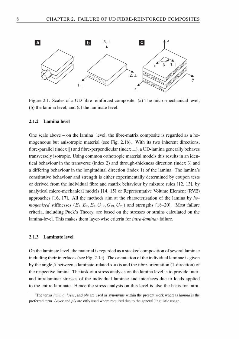
According to the setup of UD fibre-reinforced composites there are four levels on whichthe composite can be analysed.
2.1.1 Micro-mechanical level
On the smallest, the micro-mechanical level, the fibres and the matrix are treated as sepa-rate materials with different constitutive behaviour (see Fig. 2.1a). This is the level, wherefibre-matrix and fibre-fibre interactions are studied. For example the bonding betweenindividual fibres and their surrounding matrix has been investigated experimentally andnumerically [9]. Furthermore, combined numerical and experimental results concerningthe load redistribution due to successive fibre failure [10] have been incorporated into sta-tistical fibre-bundle models [11]. Regarding Puck’s failure criteria, the micro-mechaniclevel is not explicitly analysed but major mechanisms are condensed and transferred tothe lamina level (see Sec. 4.3).
8 CHAPTER 2. FAILURE OF UD FIBRE-REINFORCED COMPOSITES
3, ^
2, ^
1, ||
y
x
z
x b 1, ||
a cb
Figure 2.1: Scales of a UD fibre reinforced composite: (a) The micro-mechanical level,(b) the lamina level, and (c) the laminate level.
2.1.2 Lamina level
One scale above – on the lamina1 level, the fibre-matrix composite is regarded as a ho-mogeneous but anisotropic material (see Fig. 2.1b). With its two inherent directions,fibre-parallel (index ∥) and fibre-perpendicular (index ⊥), a UD-lamina generally behavestransversely isotropic. Using common orthotropic material models this results in an iden-tical behaviour in the transverse (index 2) and through-thickness direction (index 3) anda differing behaviour in the longitudinal direction (index 1) of the lamina. The lamina’sconstitutive behaviour and strength is either experimentally determined by coupon testsor derived from the individual fibre and matrix behaviour by mixture rules [12, 13], byanalytical micro-mechanical models [14, 15] or Representative Volume Element (RVE)approaches [16, 17]. All the methods aim at the characterisation of the lamina by ho-mogenised stiffnesses (𝐸1, 𝐸2, 𝐸3, 𝐺12, 𝐺13, 𝐺23) and strengths [18–20]. Most failurecriteria, including Puck’s Theory, are based on the stresses or strains calculated on thelamina-level. This makes them layer-wise criteria for intra-laminar failure.
2.1.3 Laminate level
On the laminate level, the material is regarded as a stacked composition of several laminaeincluding their interfaces (see Fig. 2.1c). The orientation of the individual laminae is givenby the angle 𝛽 between a laminate-related x-axis and the fibre-orientation (1-direction) ofthe respective lamina. The task of a stress analysis on the lamina level is to provide inter-and intralaminar stresses of the individual laminae and interfaces due to loads appliedto the entire laminate. Hence the stress analysis on this level is also the basis for intra-
1The terms lamina, layer, and ply are used as synonyms within the present work whereas lamina is thepreferred term. Layer and ply are only used where required due to the general linguistic usage.
2.2. TYPES OF FAILURE 9
laminar failure analysis and delamination prediction. In contrast to the lamina level, aUD fibre-reinforced lamina may react truly orthotropic when confined within a laminateregarding strength, this is called the in-situ effect (see Sec. 4.5).
2.1.4 Structural level
On the structural level, whole components are regarded. These may be of complex ge-ometry and therefore of complex local stacking sequence (see Figs. 2.8 and 2.9). Stressanalyses on the structural level provide the local state of stress at an arbitrary positionwithin the component due to the external load applied to the component. The aim ofany application-oriented failure analysis has to be a reliable failure prediction within astructural level analysis.
2.2 Types of failure
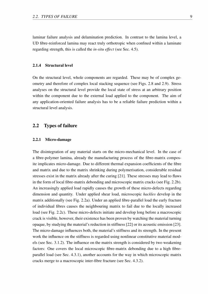
2.2.1 Micro-damage
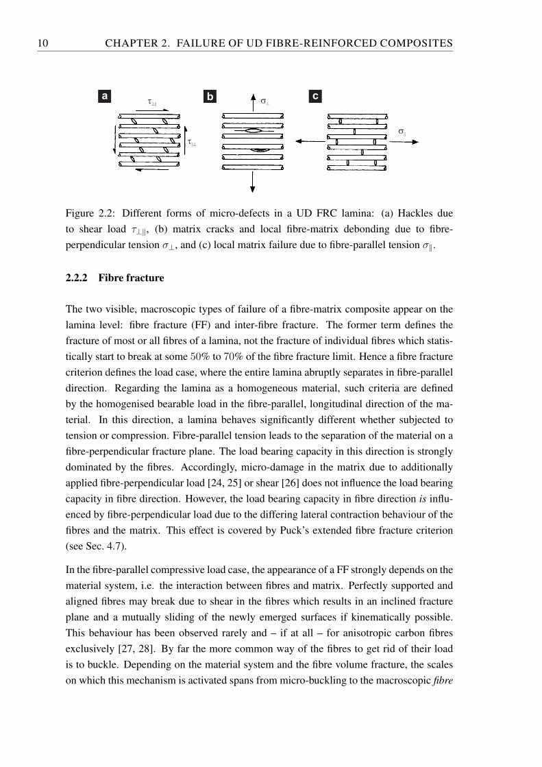
The disintegration of any material starts on the micro-mechanical level. In the case ofa fibre-polymer lamina, already the manufacturing process of the fibre-matrix compos-ite implicates micro-damage. Due to different thermal expansion coefficients of the fibreand matrix and due to the matrix shrinking during polymerisation, considerable residualstresses exist in the matrix already after the curing [21]. These stresses may lead to flawsin the form of local fibre-matrix debonding and microscopic matrix cracks (see Fig. 2.2b).An increasingly applied load rapidly causes the growth of these micro-defects regardingdimension and quantity. Under applied shear load, microscopic hackles develop in thematrix additionally (see Fig. 2.2a). Under an applied fibre-parallel load the early fractureof individual fibres causes the neighbouring matrix to fail due to the locally increasedload (see Fig. 2.2c). These micro-defects initiate and develop long before a macroscopiccrack is visible, however, their existence has been proven by watching the material turningopaque, by studying the material’s reduction in stiffness [22] or its acoustic emission [23].The micro-damage influences both, the material’s stiffness and its strength. In the presentwork the influence on the stiffness is regarded using nonlinear constitutive material mod-els (see Sec. 3.1.2). The influence on the matrix strength is considered by two weakeningfactors: One covers the local microscopic fibre-matrix debonding due to a high fibre-parallel load (see Sec. 4.3.1), another accounts for the way in which microscopic matrixcracks merge to a macroscopic inter-fibre fracture (see Sec. 4.3.2).
10 CHAPTER 2. FAILURE OF UD FIBRE-REINFORCED COMPOSITES
t^||
t||^
s||
s^
a cb
Figure 2.2: Different forms of micro-defects in a UD FRC lamina: (a) Hackles dueto shear load 𝜏⊥∥, (b) matrix cracks and local fibre-matrix debonding due to fibre-perpendicular tension 𝜎⊥, and (c) local matrix failure due to fibre-parallel tension 𝜎∥.
2.2.2 Fibre fracture
The two visible, macroscopic types of failure of a fibre-matrix composite appear on thelamina level: fibre fracture (FF) and inter-fibre fracture. The former term defines thefracture of most or all fibres of a lamina, not the fracture of individual fibres which statis-tically start to break at some 50% to 70% of the fibre fracture limit. Hence a fibre fracturecriterion defines the load case, where the entire lamina abruptly separates in fibre-paralleldirection. Regarding the lamina as a homogeneous material, such criteria are definedby the homogenised bearable load in the fibre-parallel, longitudinal direction of the ma-terial. In this direction, a lamina behaves significantly different whether subjected totension or compression. Fibre-parallel tension leads to the separation of the material on afibre-perpendicular fracture plane. The load bearing capacity in this direction is stronglydominated by the fibres. Accordingly, micro-damage in the matrix due to additionallyapplied fibre-perpendicular load [24, 25] or shear [26] does not influence the load bearingcapacity in fibre direction. However, the load bearing capacity in fibre direction is influ-enced by fibre-perpendicular load due to the differing lateral contraction behaviour of thefibres and the matrix. This effect is covered by Puck’s extended fibre fracture criterion(see Sec. 4.7).
In the fibre-parallel compressive load case, the appearance of a FF strongly depends on thematerial system, i.e. the interaction between fibres and matrix. Perfectly supported andaligned fibres may break due to shear in the fibres which results in an inclined fractureplane and a mutually sliding of the newly emerged surfaces if kinematically possible.This behaviour has been observed rarely and – if at all – for anisotropic carbon fibresexclusively [27, 28]. By far the more common way of the fibres to get rid of their loadis to buckle. Depending on the material system and the fibre volume fracture, the scaleson which this mechanism is activated spans from micro-buckling to the macroscopic fibre
2.2. TYPES OF FAILURE 11
kinking, where the fibres of large continuous regions deflect in a common direction. Incontrast to the fibre fractures due to tension, the supporting capacity of the matrix plays arole under compression. Hence the presence of matrix defects due to fibre-perpendicularor shear load influences the compressive load bearing capacity of the lamina [26] but thiseffect has not yet been incorporated into Puck’s Theory. Note that any fibre fracture inone or more laminae is currently defined as the application limit of the laminate.
2.2.3 Inter-fibre fracture
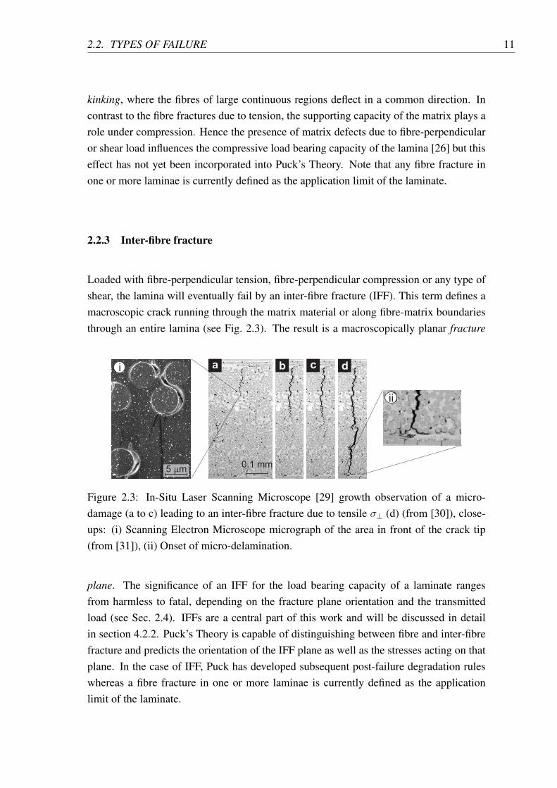
Loaded with fibre-perpendicular tension, fibre-perpendicular compression or any type ofshear, the lamina will eventually fail by an inter-fibre fracture (IFF). This term defines amacroscopic crack running through the matrix material or along fibre-matrix boundariesthrough an entire lamina (see Fig. 2.3). The result is a macroscopically planar fracture
a cb d
0.1 mm5 mm
ii
i
Figure 2.3: In-Situ Laser Scanning Microscope [29] growth observation of a micro-damage (a to c) leading to an inter-fibre fracture due to tensile 𝜎⊥ (d) (from [30]), close-ups: (i) Scanning Electron Microscope micrograph of the area in front of the crack tip(from [31]), (ii) Onset of micro-delamination.
plane. The significance of an IFF for the load bearing capacity of a laminate rangesfrom harmless to fatal, depending on the fracture plane orientation and the transmittedload (see Sec. 2.4). IFFs are a central part of this work and will be discussed in detailin section 4.2.2. Puck’s Theory is capable of distinguishing between fibre and inter-fibrefracture and predicts the orientation of the IFF plane as well as the stresses acting on thatplane. In the case of IFF, Puck has developed subsequent post-failure degradation ruleswhereas a fibre fracture in one or more laminae is currently defined as the applicationlimit of the laminate.
12 CHAPTER 2. FAILURE OF UD FIBRE-REINFORCED COMPOSITES
2.2.4 Delamination
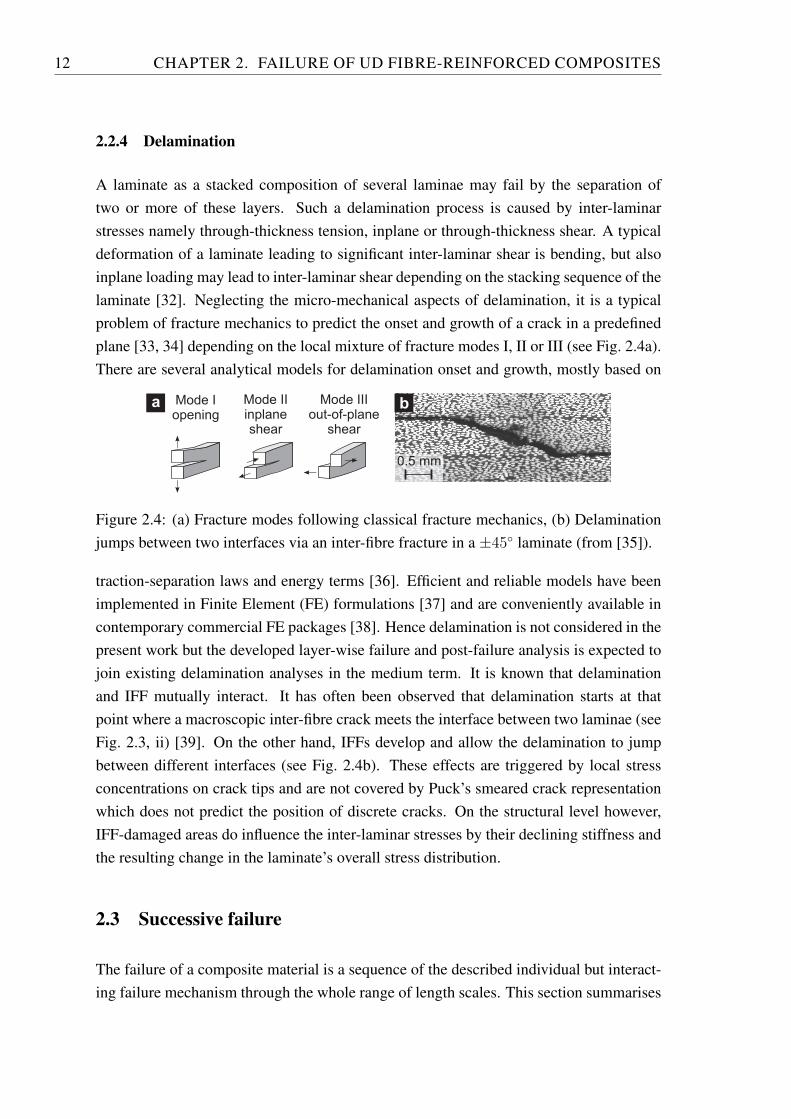
A laminate as a stacked composition of several laminae may fail by the separation oftwo or more of these layers. Such a delamination process is caused by inter-laminarstresses namely through-thickness tension, inplane or through-thickness shear. A typicaldeformation of a laminate leading to significant inter-laminar shear is bending, but alsoinplane loading may lead to inter-laminar shear depending on the stacking sequence of thelaminate [32]. Neglecting the micro-mechanical aspects of delamination, it is a typicalproblem of fracture mechanics to predict the onset and growth of a crack in a predefinedplane [33, 34] depending on the local mixture of fracture modes I, II or III (see Fig. 2.4a).There are several analytical models for delamination onset and growth, mostly based on
Mode IIinplaneshear
Mode Iopening
Mode IIIout-of-plane
shear
a b
0.5 mm
Figure 2.4: (a) Fracture modes following classical fracture mechanics, (b) Delaminationjumps between two interfaces via an inter-fibre fracture in a ±45∘ laminate (from [35]).
traction-separation laws and energy terms [36]. Efficient and reliable models have beenimplemented in Finite Element (FE) formulations [37] and are conveniently available incontemporary commercial FE packages [38]. Hence delamination is not considered in thepresent work but the developed layer-wise failure and post-failure analysis is expected tojoin existing delamination analyses in the medium term. It is known that delaminationand IFF mutually interact. It has often been observed that delamination starts at thatpoint where a macroscopic inter-fibre crack meets the interface between two laminae (seeFig. 2.3, ii) [39]. On the other hand, IFFs develop and allow the delamination to jumpbetween different interfaces (see Fig. 2.4b). These effects are triggered by local stressconcentrations on crack tips and are not covered by Puck’s smeared crack representationwhich does not predict the position of discrete cracks. On the structural level however,IFF-damaged areas do influence the inter-laminar stresses by their declining stiffness andthe resulting change in the laminate’s overall stress distribution.
2.3 Successive failure
The failure of a composite material is a sequence of the described individual but interact-ing failure mechanism through the whole range of length scales. This section summarises
2.3. SUCCESSIVE FAILURE 13
the history of events in a damaging lamina and laminate and introduces the relevant termsand definitions regarding Puck’s Theory.
2.3.1 Damage evolution in a confined lamina
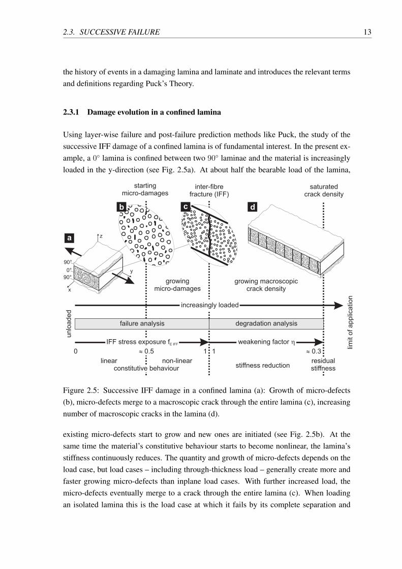
Using layer-wise failure and post-failure prediction methods like Puck, the study of thesuccessive IFF damage of a confined lamina is of fundamental interest. In the present ex-ample, a 0∘ lamina is confined between two 90∘ laminae and the material is increasinglyloaded in the y-direction (see Fig. 2.5a). At about half the bearable load of the lamina,
un
loa
de
d
limit o
f a
pp
lica
tio
n
failure analysis
inter-fibrefracture (IFF)
y
x
z
90°
0°
90°
0
IFF stress exposure fE IFF
» 0.5
growingmicro-damages
increasingly loaded
growing macroscopiccrack density
startingmicro-damages
saturatedcrack density
degradation analysis
stiffness reductionlinear non-linear
constitutive behaviourresidualstiffness
weakening factor h
11 » 0.3
a
cb d
Figure 2.5: Successive IFF damage in a confined lamina (a): Growth of micro-defects(b), micro-defects merge to a macroscopic crack through the entire lamina (c), increasingnumber of macroscopic cracks in the lamina (d).
existing micro-defects start to grow and new ones are initiated (see Fig. 2.5b). At thesame time the material’s constitutive behaviour starts to become nonlinear, the lamina’sstiffness continuously reduces. The quantity and growth of micro-defects depends on theload case, but load cases – including through-thickness load – generally create more andfaster growing micro-defects than inplane load cases. With further increased load, themicro-defects eventually merge to a crack through the entire lamina (c). When loadingan isolated lamina this is the load case at which it fails by its complete separation and
14 CHAPTER 2. FAILURE OF UD FIBRE-REINFORCED COMPOSITES
looses its entire load bearing capacity. Consistently a layer-wise criterion like Puck de-fines inter-fibre fracture meaning a macroscopic crack through the entire lamina as failureof a lamina. Although the arisen fracture plane does no longer transmit any load, in thecase of a confined lamina the neighbouring laminae still induce load into the sound sec-tions of the damaging lamina. The result is a growing number of macroscopic cracksif more load is applied (see Fig. 2.5d). The amount of load which is induced into andhence carried by the damaging lamina depends on the size of the sound sections. Accord-ingly, with a growing macroscopic crack density, the portion of the applied load whichis carried by the damaging lamina reduces and more and more load is redistributed tothe neighbouring laminae. At a specific crack density – the saturated crack density, thesound sections of the damaging lamina have become so small that the induced load is nolonger sufficient for producing further cracks. At this point the damage development inthe considered lamina is completed, even if more load is applied.
Following Puck’s Theory, the prediction of the whole damage development consists oftwo parts: the failure analysis and the post failure degradation analysis. The former eval-uates a state of stress regarding fibre and – in the present example – inter-fibre fracture.The central parameter is the IFF stress exposure 𝑓𝐸 𝐼𝐹𝐹 running linearly from 0 (un-loaded) to 1 (inter-fibre fracture) with linearly increasing stresses. Micro-damage startsat a value of 𝑓𝐸 𝐼𝐹𝐹 ≈ 0.5 and its influence on the load bearing capacity is regarded byweakening factors (see Sec. 4.3). The failure analysis is preferably based on a nonlinearstress analysis which includes the effects of micro-defects on the material’s stiffness (seeSec. 3.1.2). Having reached the IFF limit, in the subsequent post failure degradation anal-ysis the material’s stiffness is reduced according to the applied load or the resulting crackdensity respectively. A central measure is the weakening factor 𝜂 which develops from1 (no stiffness reduction) to exemplary 0.3 (residual stiffness) when having reached thesaturated crack density. Regarding the numerical realisation the failure analysis is a post-processing of calculated stresses which means it can independently follow any kind ofstress analysis. The degradation analysis, however, is constantly changing the material’sconstitutive behaviour and therefore stress and degradation analysis are two mutually in-teracting parts of a numerical prediction beyond IFF.
2.3.2 Successive failure of a laminate
The successive damage of a balanced 0∘/90∘ laminate loaded in the y-direction (seeFig. 2.6) is representative for the complex and interacting failure process of UD fibre-reinforced composites. Loaded inplane by a tensile load 𝐹 , the first damage occurs inthe 0∘ laminae where fibre-transverse tensile 𝜎𝑡2 ⊥ produces the first ply failure in form
2.4. FAILURE ON THE STRUCTURAL LEVEL 15
a cb
y
x
z
F
F
y
x
z
F
F
y
x
z
F
F
90°
0°
0°
90°
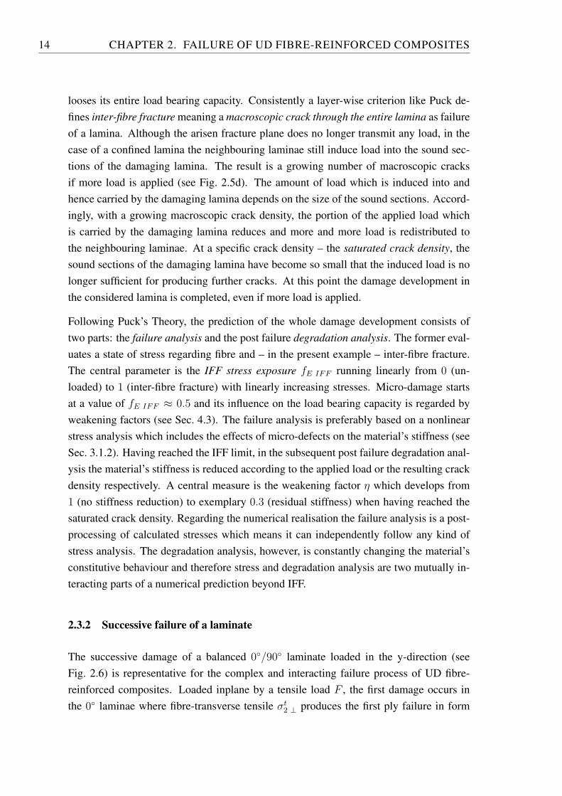
Figure 2.6: Section of a balanced 0∘/90∘ laminate increasingly loaded: first ply failureIFFs in the 0∘ laminae (a), second ply failure IFFs in the 90∘ laminae (b) and third plyfailure FFs in the 90∘ laminae (c).
of vertical IFFs (𝜃𝑓𝑝 = 0∘). Increasingly loaded, in the 0∘ laminae develop more andmore IFFs (see Fig. 2.6a) going along with the decrease of stiffness – the degradation –of these laminae. The result is a load redistribution from the damaging laminae to theneighbouring ones. Accordingly the tensile 𝜎𝑡1 ∥ in the 90∘ laminae increases togetherwith the laminae’s lateral contraction due to the Poisson’s effect. Impeded by the fibresof the 0∘ laminae (they carry compressive 𝜎𝑐1 ∥), the result is a fibre-transverse tension𝜎𝑡2 ⊥ in the 90∘ laminae producing the second ply failure: vertical IFFs in the 90∘ laminae(b). Still capable of bearing the load 𝐹 , the laminate may be increasingly loaded until thefollowing fibre fractures in the 90∘ laminae mark the third ply failure and the final failureof the laminate (c). This example proves the importance of the distinction between fibrefracture (FF) and inter-fibre fracture (IFF) regarding failure analysis in a damage-tolerantdesign process.
2.4 Failure on the structural level
The aim of any failure analysis is the prediction of when the application limit of a materialor a component will be reached. The definitions of these limits are as widespread as thefields of application of fibre-reinforced composites or as their successive modes of failure.
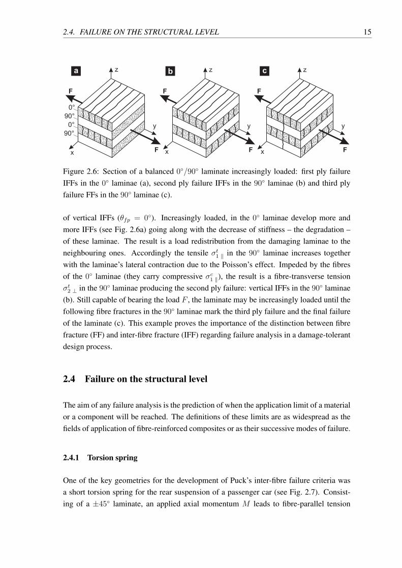
2.4.1 Torsion spring
One of the key geometries for the development of Puck’s inter-fibre failure criteria wasa short torsion spring for the rear suspension of a passenger car (see Fig. 2.7). Consist-ing of a ±45∘ laminate, an applied axial momentum 𝑀 leads to fibre-parallel tension
16 CHAPTER 2. FAILURE OF UD FIBRE-REINFORCED COMPOSITES
𝜎𝑡1 ∥ together with fibre-transverse compression 𝜎𝑐2 ⊥ in the outer lamina (white) and tofibre-parallel compression 𝜎𝑐1 ∥ together with fibre-transverse tension 𝜎𝑡2 ⊥ in the innerlamina (grey). Repeatedly loaded, the inter-fibre fractures (IFFs) in the inner lamina (see
Mtyx
txy
txy
tyx
s s1 2
c t
|| ^,
txy
s s1 2
t c
|| ^,
tyx
txy
tyxs2
c
^
s2
t
^
a
b
q »fp 54°
Figure 2.7: Torsion spring made of UD Glass Fibre Reinforced Composite (GFRC): (a)Fatal and (b) tolerable inter-fibre fracture (IFF).
Fig. 2.7b) turned out to be completely harmless for the structure and its load bearing ca-pacity although these fractures had already occurred in large numbers after few cycles.After the crack density of these cracks had reached its saturation, the spring survived 106
cycles as long as no IFF in the outer lamina occurred. In contrast to this a single IFF in theouter lamina immediately led to the total failure of the complete structure (see Fig. 2.7a).The inclined fracture plane (𝜃𝑓𝑝 ≈ 54∘) transmitting pressure leads to the wedge effectwhere parts of the transmitted forces are deflected in trough-thickness direction. In thepresent case these forces in positive and negative radial direction either cause the innerlamina to collapse or the outer lamina to be blasted – both with the result of an immediatetotal collapse of the loaded spring [4, 39, 40]. Although the example above is a fatigue ex-periment and is hence far beyond the failure prediction topic and the scope of the presentwork, it proves the importance of the distinction between different modes of inter-fibrefracture.
2.4.2 Integral vehicle rear suspension
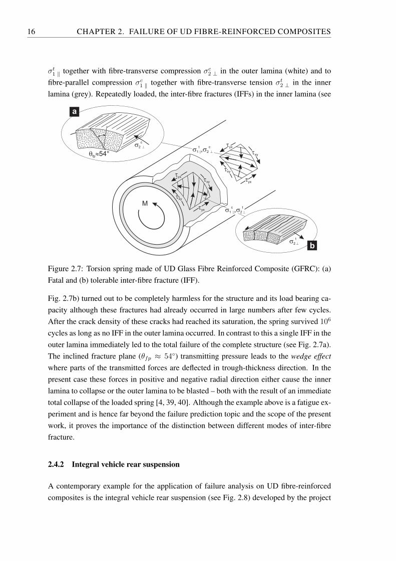
A contemporary example for the application of failure analysis on UD fibre-reinforcedcomposites is the integral vehicle rear suspension (see Fig. 2.8) developed by the project
2.4. FAILURE ON THE STRUCTURAL LEVEL 17
Aktives Leichtbaufahrwerk (Active Lightweight chassis) of the German Bundesminis-terium fur Bildung und Forschung (BMBF – Federal Ministry of Education and Research).The aim is a lighter chassis due to the application of lightweight, multifunctional andadaptive materials and the integration of currently a large number of structural assembliesinto a single suspension component. The fact that one single component is intended to
Figure 2.8: Starting point for the future integral vehicle rear suspension: Wheel-guidingtransverse leaf spring axle (grey) made of fibre-reinforced composite (FRC), additionallyvisible suspension components (white) are to be integrated into the final construction(from [41]).
transmit forces between the wheels and the vehicle and at the same time to cushion theseforces leads to a particularly narrow design space regarding stiffness [42]. Attached to apassenger car, the customer requires maintenance-free components without the need forhealth monitoring. Hence the design space regarding strength is also limited since a finitelife, damage-tolerant design is excluded. In this project a stress analysis by Finite ElementMethod (FEM) combined with a failure analysis based on Puck’s Theory could identifythe overlapping of the two design spaces mentioned. This example proves the need for anaccurate damage initiation analysis including reliable information about the safety factor.
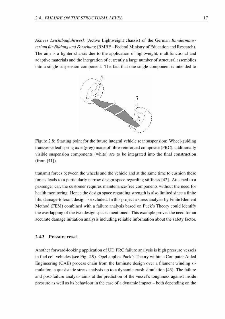
2.4.3 Pressure vessel
Another forward-looking application of UD FRC failure analysis is high pressure vesselsin fuel cell vehicles (see Fig. 2.9). Opel applies Puck’s Theory within a Computer AidedEngineering (CAE) process chain from the laminate design over a filament winding si-mulation, a quasistatic stress analysis up to a dynamic crash simulation [43]. The failureand post-failure analysis aims at the prediction of the vessel’s toughness against insidepressure as well as its behaviour in the case of a dynamic impact – both depending on the
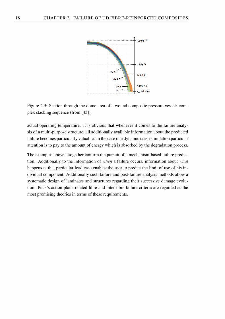
18 CHAPTER 2. FAILURE OF UD FIBRE-REINFORCED COMPOSITES
X / mm
cyl
po
Figure 2.9: Section through the dome area of a wound composite pressure vessel: com-plex stacking sequence (from [43]).
actual operating temperature. It is obvious that whenever it comes to the failure analy-sis of a multi-purpose structure, all additionally available information about the predictedfailure becomes particularly valuable. In the case of a dynamic crash simulation particularattention is to pay to the amount of energy which is absorbed by the degradation process.
The examples above altogether confirm the pursuit of a mechanism-based failure predic-tion. Additionally to the information of when a failure occurs, information about whathappens at that particular load case enables the user to predict the limit of use of his in-dividual component. Additionally such failure and post-failure analysis methods allow asystematic design of laminates and structures regarding their successive damage evolu-tion. Puck’s action plane-related fibre and inter-fibre failure criteria are regarded as themost promising theories in terms of these requirements.
3 3D stress analysis in laminates and structures
According to the multiscale character of the material (see Sec. 2.1) the task of a stressanalysis is related to the respective level. On the lamina level the stress analysis assigns astate of stress to any state of strain or vice versa, i.e. this is the level where the constitutivebehaviour of the individual lamina is interpreted (see Sec. 3.1). On the laminate level thestress analysis determines the distribution of load among the involved laminae due toloads which are applied to the laminate material as a whole. This may happen as part ofan analysis on the structural level whose task is the determination of the local states ofstress and strain at an arbitrary position of the structure due to loads which are appliedon specific positions in the form of forces or displacements (see Sec. 3.3.2). The secondimportant application of the stress analysis on the laminate level is the determination ofgeneralised laminate behaviour. In that context the presented RVE approach replacesthe established Classical Laminate Theory (CLT) in the case of applied 3D loads (seeSec. 3.5). The mentioned levels are hierarchical in the sense that analysis on a higher levelrequire all those on the levels below. In the following sections the theoretical and practicalaspects of the stress analysis are treated whereas the primary attention is drawn to theapplication within a Finite Element Analysis (see Sec. 3.2) – the commercial FE packageABAQUS [8] in particular (see Sec. 3.3). Furthermore the quality of the presented FErepresentations is determined by the comparison with the analytical solution followingPagano (see Sec. 3.4) and considerations about geometric nonlinearity (see Sec. 3.6) andthermally induced residual stresses are presented (see Sec. 3.7).
3.1 Constitutive behaviour of a lamina
3.1.1 Transverse isotropy and orthotropy
Neglecting mechanism on smaller scales the individual lamina is regarded as an homoge-neous but anisotropic material (see Sec. 2.1). In the undamaged state it behaves equallyin the transverse 2-direction and the through-thickness 3-direction which allows to reducethe general anisotropy to a transversely isotropic behaviour with only a fibre-parallel ∥and fibre-perpendicular ⊥ direction (see Fig. 2.1b). The constitutive behaviour, i.e. thematerial law which relates states of stress to states of strain is then defined by the compli-
20 CHAPTER 3. 3D STRESS ANALYSIS IN LAMINATES AND STRUCTURES
ance matrix 𝑆 in Voight notation:
⎡⎢⎢⎢⎢⎢⎢⎢⎢⎣
𝜖1
𝜖2
𝜖3
𝛾12
𝛾13
𝛾23
⎤⎥⎥⎥⎥⎥⎥⎥⎥⎦=
⎡⎢⎢⎢⎢⎢⎢⎢⎢⎣
1/𝐸∥ −𝜈⊥∥/𝐸⊥ −𝜈⊥∥/𝐸⊥ 0 0 0
−𝜈∥⊥/𝐸∥ 1/𝐸⊥ −𝜈⊥⊥/𝐸⊥ 0 0 0
−𝜈∥⊥/𝐸∥ −𝜈⊥⊥/𝐸⊥ 1/𝐸⊥ 0 0 0
0 0 0 1/𝐺∥⊥ 0 0
0 0 0 0 1/𝐺∥⊥ 0
0 0 0 0 0 1/𝐺⊥⊥
⎤⎥⎥⎥⎥⎥⎥⎥⎥⎦⋅
⎡⎢⎢⎢⎢⎢⎢⎢⎢⎣
𝜎1
𝜎2
𝜎3
𝜏12
𝜏13
𝜏23
⎤⎥⎥⎥⎥⎥⎥⎥⎥⎦(3.1)
A 3D state of stress 𝜎 consists of three normal stresses 𝜎𝑖 and three shear stresses 𝜏𝑖𝑗 ,accordingly a 3D state of strain 𝜖 of three normal strains 𝜖𝑖 and three shear strains 𝛾𝑖𝑗 . Thematerial is characterised by common engineering constants namely Young’s moduli 𝐸𝑖and shear moduli𝐺𝑖𝑗
1 and the quantities 𝜈𝑖𝑗 . The latter have the physical interpretation ofPoisson’s ratios that characterise the transverse strain in the 𝑗-direction, when the materialis stressed in the 𝑖-direction. In general, 𝜈𝑖𝑗 is not equal to 𝜈𝑗𝑖 – they are related by𝜈𝑖𝑗/𝐸𝑖 = 𝜈𝑗𝑖/𝐸𝑗 .
For the pure failure analysis of a UD fibre reinforced composite (see Ch. 4), the trans-versely isotropic material description is generally adequate but within the post-failuredegradation process the lamina starts to behave truly orthotropic if not completelyanisotropic (see Ch. 5). Whereas the latter behaviour is currently academic (see Sec. 5.6)the orthotropic material model (see Eq. 3.2) is set to the standard for the implementationdeveloped within this work (see Ch. 6) and for 3D stress analyses of laminae in general.
⎡⎢⎢⎢⎢⎢⎢⎢⎢⎣
𝜖1
𝜖2
𝜖3
𝛾12
𝛾13
𝛾23
⎤⎥⎥⎥⎥⎥⎥⎥⎥⎦=
⎡⎢⎢⎢⎢⎢⎢⎢⎢⎣
1/𝐸1 −𝜈21/𝐸2 −𝜈31/𝐸3 0 0 0
−𝜈12/𝐸1 1/𝐸2 −𝜈32/𝐸2 0 0 0
−𝜈13/𝐸1 −𝜈23/𝐸3 1/𝐸⊥ 0 0 0
0 0 0 1/𝐺12 0 0
0 0 0 0 1/𝐺13 0
0 0 0 0 0 1/𝐺23
⎤⎥⎥⎥⎥⎥⎥⎥⎥⎦⋅
⎡⎢⎢⎢⎢⎢⎢⎢⎢⎣
𝜎1
𝜎2
𝜎3
𝜏12
𝜏13
𝜏23
⎤⎥⎥⎥⎥⎥⎥⎥⎥⎦(3.2)
Being a displacement-based approach a FE analysis requires a material description in theform of 𝜎 (𝜖) = 𝐸 ⋅ 𝜖 (see Ch. 6) whereas the stiffness matrix 𝐸 is the inverse of the
1Within the present work Young’s moduli and shear moduli are addressed together by the term stiff-nesses.
3.1. CONSTITUTIVE BEHAVIOUR OF A LAMINA 21
compliance matrix 𝑆 (see Eq. 3.3).⎡⎢⎢⎢⎢⎢⎢⎢⎢⎣
𝜎1
𝜎2
𝜎3
𝜏12
𝜏13
𝜏23
⎤⎥⎥⎥⎥⎥⎥⎥⎥⎦=
⎡⎢⎢⎢⎢⎢⎢⎢⎢⎣
𝐷1111 𝐷1122 𝐷1133 0 0 0
𝐷2222 𝐷2233 0 0 0
𝐷3333 0 0 0
𝐷1212 0 0
sym. 𝐷1313 0
𝐷2323
⎤⎥⎥⎥⎥⎥⎥⎥⎥⎦⋅
⎡⎢⎢⎢⎢⎢⎢⎢⎢⎣
𝜖1
𝜖2
𝜖3
𝛾12
𝛾13
𝛾23
⎤⎥⎥⎥⎥⎥⎥⎥⎥⎦(3.3)
The components of 𝐸 are
𝐷1111 =𝐸1 (1− 𝜈23𝜈32)Υ
𝐷2222 =𝐸2 (1− 𝜈13𝜈31)Υ
𝐷3333 =𝐸3 (1− 𝜈12𝜈21)Υ
𝐷1122 =𝐸1 (𝜈21 + 𝜈31𝜈23)Υ = 𝐸2 (𝜈12 + 𝜈32𝜈13)Υ
𝐷1133 =𝐸1 (𝜈31 + 𝜈21𝜈32)Υ = 𝐸3 (𝜈13 + 𝜈12𝜈23)Υ
𝐷2233 =𝐸2 (𝜈32 + 𝜈12𝜈31)Υ = 𝐸3 (𝜈23 + 𝜈21𝜈13)Υ
𝐷1212 =𝐺12
𝐷1313 =𝐺13
𝐷2323 =𝐺23
(3.4)
whereΥ =
1
1− 𝜈12𝜈21 − 𝜈23𝜈32 − 𝜈13𝜈31 − 2𝜈21𝜈32𝜈13. (3.5)
The stability restrictions on the engineering constants are
𝐸1, 𝐸2, 𝐸3, 𝐺12, 𝐺13, 𝐺23 > 0
∣𝜈12∣ < (𝐸1/𝐸2)1/2 or ∣𝜈21∣ < (𝐸2/𝐸1)
1/2
∣𝜈13∣ < (𝐸1/𝐸3)1/2 or ∣𝜈31∣ < (𝐸3/𝐸1)
1/2
∣𝜈23∣ < (𝐸2/𝐸3)1/2 or ∣𝜈32∣ < (𝐸3/𝐸2)
1/2
1− 𝜈12𝜈21 − 𝜈23𝜈32 − 𝜈13𝜈31 − 2𝜈21𝜈32𝜈13 > 0 .
(3.6)
3.1.2 Nonlinearities in the constitutive behaviour
In contrast to the nonlinear elastic-plastic behaviour of metals a suitable nonlinear or-thotropic material model for glass- or carbon-fibre polymer-matrix composites is not com-monly included in contemporary FEA packages. It is however straightforward to includeat least those nonlinear stress-strain relations which are determined by uniaxial material
22 CHAPTER 3. 3D STRESS ANALYSIS IN LAMINATES AND STRUCTURES
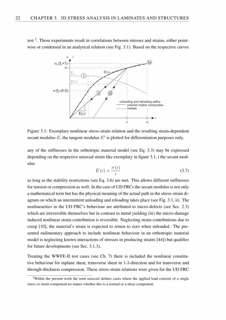
test 2. Those experiments result in correlations between stresses and strains, either point-wise or condensed in an analytical relation (see Fig. 3.1). Based on the respective curves
s
s »E(f 0.5)
E( )e
E( )te
E
Elin
E( )e
ii
i
iii
unloading and reloading paths:polymer-matrix compositesmetalls
e
s
e efr
sfr E(f =1) iv
Figure 3.1: Exemplary nonlinear stress-strain relation and the resulting strain-dependentsecant modulus 𝐸, the tangent modulus 𝐸𝑡 is plotted for differentiation purposes only.
any of the stiffnesses in the orthotripic material model (see Eq. 3.3) may be expresseddepending on the respective uniaxial strain like exemplary in figure 3.1, i the secant mod-ulus
𝐸 (𝜖) =𝜎 (𝜖)
𝜖(3.7)
as long as the stability restrictions (see Eq. 3.6) are met. This allows different stiffnessesfor tension or compression as well. In the case of UD FRCs the secant modulus is not onlya mathematical term but has the physical meaning of the actual path in the stress-strain di-agram on which an intermittent unloading and reloading takes place (see Fig. 3.1, ii). Thenonlinearities in the UD FRC’s behaviour are attributed to micro-defects (see Sec. 2.3)which are irreversible themselves but in contrast to metal yielding (iii) the micro-damageinduced nonlinear strain contribution is reversible. Neglecting strain contributions due tocreep [10], the material’s strain is expected to return to zero when unloaded. The pre-sented rudimentary approach to include nonlinear behaviour in an orthotropic materialmodel is neglecting known interactions of stresses in producing strains [44]) but qualifiesfor future developments (see Sec. 3.1.3).
Treating the WWFE-II test cases (see Ch. 7) there is included the nonlinear constitu-tive behaviour for inplane shear, transverse shear in 1-3-direction and for transverse andthrough-thickness compression. These stress-strain relations were given for the UD FRC
2Within the present work the term uniaxial defines cases where the applied load consists of a singlestress or strain component no matter whether this is a normal or a shear component.
3.1. CONSTITUTIVE BEHAVIOUR OF A LAMINA 23
material (see App. B). Where the nonlinear constitutive behaviours of the fibres and thematrix were given separately, the application of mixture rules was judged to be less reli-able than using the linear relations.
3.1.3 Interaction between transverse and shear deformation
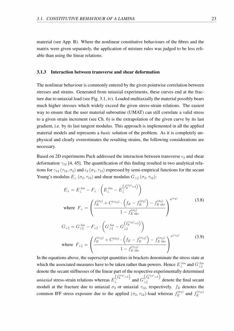
The nonlinear behaviour is commonly entered by the given pointwise correlation betweenstresses and strains. Generated from uniaxial experiments, these curves end at the frac-ture due to uniaxial load (see Fig. 3.1, iv). Loaded multiaxially the material possibly bearsmuch higher stresses which widely exceed the given stress-strain relations. The easiestway to ensure that the user material subroutine (UMAT) can still correlate a valid stressto a given strain increment (see Ch. 6) is the extrapolation of the given curve by its lastgradient, i.e. by its last tangent modulus. This approach is implemented in all the appliedmaterial models and represents a basic solution of the problem. As it is completely un-physical and clearly overestimates the resulting strains, the following considerations arenecessary.
Based on 2D experiments Puck addressed the interaction between transverse 𝜖2 and sheardeformation 𝛾12 [4, 45]. The quantification of this finding resulted in two analytical rela-tions for 𝛾12 (𝜏12, 𝜎2) and 𝜖2 (𝜎2, 𝜏12) expressed by semi-empirical functions for the secantYoung’s modulus 𝐸⊥ (𝜎2, 𝜏12) and shear modulus 𝐺⊥∥ (𝜎2, 𝜏12):
𝐸⊥ = 𝐸 𝑙𝑖𝑛⊥ − 𝐹⊥ ⋅
(𝐸 𝑙𝑖𝑛
⊥ − 𝐸
(𝑓(𝜎2)𝐸 =1
)⊥
)
where 𝐹⊥ =
⎛⎝𝑓 (𝜎2)𝐸 + 𝐶(𝜏12) ⋅
(𝑓𝐸 − 𝑓
(𝜎2)𝐸
)− 𝑓
(𝜎2)𝐸 𝑡ℎ𝑟
1− 𝑓(𝜎2)𝐸 𝑡ℎ𝑟
⎞⎠𝑛(𝜎2) (3.8)
𝐺⊥∥ = 𝐺 𝑙𝑖𝑛⊥∥ − 𝐹⊥∥ ⋅
(𝐺 𝑙𝑖𝑛
⊥∥ −𝐺
(𝑓(𝜏12)𝐸 =1
)⊥∥
)
where 𝐹⊥∥ =
⎛⎝𝑓 (𝜏12)𝐸 + 𝐶(𝜎2) ⋅
(𝑓𝐸 − 𝑓
(𝜏12)𝐸
)− 𝑓
(𝜏12)𝐸 𝑡ℎ𝑟
1− 𝑓(𝜏12)𝐸 𝑡ℎ𝑟
⎞⎠𝑛(𝜏12) (3.9)
In the equations above, the superscript quantities in brackets denominate the stress state atwhich the associated measures have to be taken rather than powers. Hence 𝐸 𝑙𝑖𝑛
⊥ and 𝐺 𝑙𝑖𝑛⊥∥
denote the secant stiffnesses of the linear part of the respective experimentally determined
uniaxial stress-strain relations whereas 𝐸
(𝑓(𝜎2)𝐸 =1
)⊥ and 𝐺
(𝑓(𝜏12)𝐸 =1
)⊥∥ denote the final secant
moduli at the fracture due to uniaxial 𝜎2 or uniaxial 𝜏12, respectively. 𝑓𝐸 denotes thecommon IFF stress exposure due to the applied (𝜎2, 𝜏12)-load whereas 𝑓 (𝜎2)
𝐸 and 𝑓 (𝜏12)𝐸
24 CHAPTER 3. 3D STRESS ANALYSIS IN LAMINATES AND STRUCTURES
denote the IFF stress exposure due to the isolated 𝜎2-component or due to the isolated𝜏12-component, respectively. The rest of the parameters in equations 3.8 and 3.9 havebeen experimentally derived [23, 26]:
CFRC GFRC(𝜎2) (𝜏12) (𝜎2) (𝜏12)
𝑓𝐸 𝑡ℎ𝑟 0.3 0.3 0.3 0.3𝑛 2.5 1.7 3.0 2.0𝐶 0.6 0.6 0.6 0.6
Table 3.1: Parameters for the inplane transverse and shear deformation interaction [4].
These resulting stress-strain-curves perfectly reproduce the experimental results for thestress ratios under consideration 𝜎2/∣𝜏21∣ = [−2; 1] and are valid up to fracture due tocombined load. The physical background of this approach is the idea that nonlinearitiesin fibre/polymer composites result from cumulative micromechanical damage [23]. If acombined load leads to higher bearable stresses in terms of macroscopic fracture, it isreasonable to expect the influence of micro-damage also being shifted to higher stresslevels. Mainly based on the ratios between the stress exposure due to uniaxial load 𝑓 (𝜏21)
𝐸
or 𝑓 (𝜎2)𝐸 , respectively and the stress exposure due to the combined load 𝑓𝐸 , the approach
is generally transferable into 3D space.
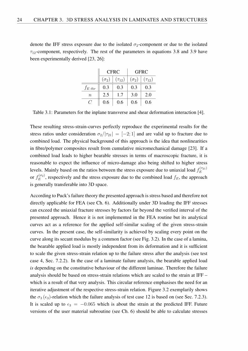
According to Puck’s failure theory the presented approach is stress based and therefore notdirectly applicable for FEA (see Ch. 6). Additionally under 3D loading the IFF stressescan exceed the uniaxial fracture stresses by factors far beyond the verified interval of thepresented approach. Hence it is not implemented in the FEA routine but its analyticalcurves act as a reference for the applied self-similar scaling of the given stress-straincurves. In the present case, the self-similarity is achieved by scaling every point on thecurve along its secant modulus by a common factor (see Fig. 3.2). In the case of a lamina,the bearable applied load is mostly independent from its deformation and it is sufficientto scale the given stress-strain relation up to the failure stress after the analysis (see testcase 4, Sec. 7.2.2). In the case of a laminate failure analysis, the bearable applied loadis depending on the constitutive behaviour of the different laminae. Therefore the failureanalysis should be based on stress-strain relations which are scaled to the strain at IFF –which is a result of that very analysis. This circular reference emphasises the need for aniterative adjustment of the respective stress-strain relation. Figure 3.2 exemplarily showsthe 𝜎3 (𝜖3)-relation which the failure analysis of test case 12 is based on (see Sec. 7.2.3).It is scaled up to 𝜖3 = −0.065 which is about the strain at the predicted IFF. Futureversions of the user material subroutine (see Ch. 6) should be able to calculate stresses
3.2. FE REPRESENTATION OF LAMINATES AND LAMINATE STRUCTURES 25
[ ]
[
]
Figure 3.2: Scaled self-similar constitutive behaviour in through-thickness direction fortest case 12 (residual stresses neglected).
from stress-strain relations, which have been scaled according to information availablefrom the preceding load increment.
3.2 FE representation of laminates and laminate structures
Laminates and laminate structures commonly have geometries with small thicknessescompared to their lateral expansion. Accordingly there is the legitimate desire to representthe three-dimensional continuum by a condensed two-dimensional structural model [46].The governing equations and the associated boundary conditions of the reduced modelare than derived upon an elimination of the thickness coordinate by integrating alongthe thickness the partial differential equations of the three-dimensional continuum [47].A large number of theories and associated finite element definitions have been createdover the years to achieve the compliance with the basic requirements for the stress, strainand displacement fields over a laminate’s through-thickness direction (see Secs. 3.2.1 and3.2.2).
The considerations about the slope and the boundary conditions of stress and strain fieldsthroughout the laminate’s thickness is based on the perception of a laminate as a stack ofdifferent homogeneous and anisotropic layers which are perfectly bonded together. Sincethe mechanical properties of the interfaces are neglected, the interlaminar boundaries aresurfaces of abrupt discontinuities in the material properties. The perfect bond conditionrequires a continuous displacement field 𝑢 over the bi-material interface and a continuousthrough-thickness stress and shear stress field 𝜎𝑧, 𝜏𝑥𝑧 and 𝜏𝑦𝑧 is required for equilibriumreasons. This results in a discontinuity in the through-thickness strain and shear strain
26 CHAPTER 3. 3D STRESS ANALYSIS IN LAMINATES AND STRUCTURES
fields 𝜖𝑧, 𝛾𝑥𝑧 and 𝛾𝑦𝑧 due to the difference in elastic properties of the adjoining layers. Asa consequence the through-thickness displacement 𝑢𝑧 has a slope discontinuity across theinterface.
The continuous displacement field over the interface results in continuous inplane strainsand shear strains 𝜖𝑥, 𝜖𝑥 and 𝛾𝑥𝑦 which results in discontinuous inplane stresses and shearstresses 𝜎𝑥, 𝜎𝑦 and 𝜏𝑥𝑦 due to the difference in elastic properties of the adjoining layers.Hence through-thickness shear stresses 𝜏𝑥𝑧 and 𝜏𝑦𝑧 generally have a slope discontinu-ity in their through-thickness distribution due to equilibrium reasons. On the contrarythe continuity of the interlaminar through-thickness shear stresses 𝜏𝑥𝑧 and 𝜏𝑦𝑧 force thethrough-thickness stress 𝜎𝑧 to have a continuous derivative along the through-thicknesscoordinate [48].
behaviour overslope
slopebi-material interface continuity
displacements𝑢𝑥, 𝑢𝑦 cont. kink𝑢𝑧 cont. kink
strains
𝜖𝑥, 𝜖𝑦 cont.𝜖𝑧 jump𝛾𝑥𝑦 cont.
𝛾𝑥𝑧, 𝛾𝑦𝑧 jump
stresses
𝜎𝑥, 𝜎𝑦 jump𝜎𝑧 cont. cont.𝜏𝑥𝑦 jump
𝜏𝑥𝑧, 𝜏𝑦𝑧 cont. kink
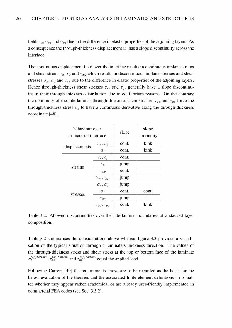
Table 3.2: Allowed discontinuities over the interlaminar boundaries of a stacked layercomposition.
Table 3.2 summarises the considerations above whereas figure 3.3 provides a visuali-sation of the typical situation through a laminate’s thickness direction. The values ofthe through-thickness stress and shear stress at the top or bottom face of the laminate𝜎𝑡𝑜𝑝/𝑏𝑜𝑡𝑡𝑜𝑚𝑧 , 𝜏 𝑡𝑜𝑝/𝑏𝑜𝑡𝑡𝑜𝑚𝑥𝑧 and 𝜏 𝑡𝑜𝑝/𝑏𝑜𝑡𝑡𝑜𝑚𝑦𝑧 equal the applied load.
Following Carrera [49] the requirements above are to be regarded as the basis for thebelow evaluation of the theories and the associated finite element definitions – no mat-ter whether they appear rather academical or are already user-friendly implemented incommercial FEA codes (see Sec. 3.3.2).
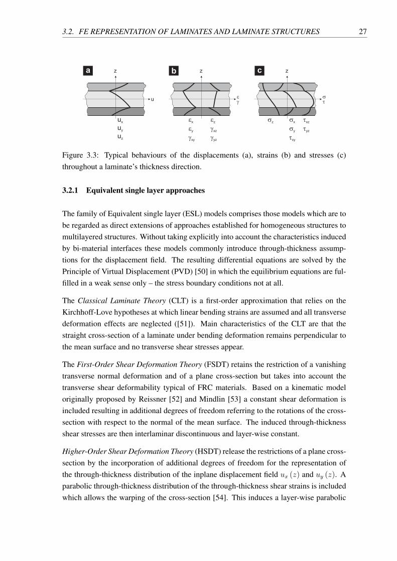
3.2. FE REPRESENTATION OF LAMINATES AND LAMINATE STRUCTURES 27
a cbz z z
u seg t
u
u
u
x
y
z
txz
tyz
s
t
x
xy
sy
szex
e
gy
xy
e
g
g
z
xz
yz
Figure 3.3: Typical behaviours of the displacements (a), strains (b) and stresses (c)throughout a laminate’s thickness direction.
3.2.1 Equivalent single layer approaches
The family of Equivalent single layer (ESL) models comprises those models which are tobe regarded as direct extensions of approaches established for homogeneous structures tomultilayered structures. Without taking explicitly into account the characteristics inducedby bi-material interfaces these models commonly introduce through-thickness assump-tions for the displacement field. The resulting differential equations are solved by thePrinciple of Virtual Displacement (PVD) [50] in which the equilibrium equations are ful-filled in a weak sense only – the stress boundary conditions not at all.
The Classical Laminate Theory (CLT) is a first-order approximation that relies on theKirchhoff-Love hypotheses at which linear bending strains are assumed and all transversedeformation effects are neglected ([51]). Main characteristics of the CLT are that thestraight cross-section of a laminate under bending deformation remains perpendicular tothe mean surface and no transverse shear stresses appear.
The First-Order Shear Deformation Theory (FSDT) retains the restriction of a vanishingtransverse normal deformation and of a plane cross-section but takes into account thetransverse shear deformability typical of FRC materials. Based on a kinematic modeloriginally proposed by Reissner [52] and Mindlin [53] a constant shear deformation isincluded resulting in additional degrees of freedom referring to the rotations of the cross-section with respect to the normal of the mean surface. The induced through-thicknessshear stresses are then interlaminar discontinuous and layer-wise constant.
Higher-Order Shear Deformation Theory (HSDT) release the restrictions of a plane cross-section by the incorporation of additional degrees of freedom for the representation ofthe through-thickness distribution of the inplane displacement field 𝑢𝑥 (𝑧) and 𝑢𝑦 (𝑧). Aparabolic through-thickness distribution of the through-thickness shear strains is includedwhich allows the warping of the cross-section [54]. This induces a layer-wise parabolic
28 CHAPTER 3. 3D STRESS ANALYSIS IN LAMINATES AND STRUCTURES
𝑧-distribution3 of the through-thickness shear stresses whereas the required shear stressconditions at the top and bottom surface of the laminate can be satisfied by an appropriatechoice of the thickness polynomials. In particular third-order shear deformation theorieshave attained a wide acceptance [55].
Theories including transverse normal deformation overcome the simplification of the the-ories presented above concerning 𝜖𝑧 = 0. This kind of theories are usually based on HSDTbut take into account the full 3D constitutive law [56, 57]. Most kinematic models assumea quadratic through-thickness distribution of the displacement 𝑢𝑧 (𝑧) which results in lin-ear through-thickness strain 𝜖𝑧 whereas the expansion of the inplane displacements hasbeen based on polynomials of different order.
The approaches presented above either neglect through-thickness strain fields 𝜖𝑧 or forcethem to be continuous in the z-direction and are thus not capable of exactly fulfilling thethrough-thickness equilibrium at the bi-material interface. Rigorously judged, the appli-cation of ESL models is restricted to the analysis of the global response of the laminate[58, 59], but the through-thickness stress and shear predictions of acceptable accuracy canbe obtained by post-processing operations [60–62].
3.2.2 Layer-wise approach
Assuming a separate displacement field for each layer – i.e. layer-wise (LW) – is astraightforward approach to explicitly account for the heterogeneos cross-section of alaminate. On the laminate level, the expressions of the layer-wise assumptions are as-sembled without enforcing a continuous through-thickness strain field. This leaves thepossibility for the through-thickness normal and shear stresses to be continuous at the bi-material interfaces. However not all the requirements of table 3.2 are automatically metby solely displacement-based layer-wise formulations. For example a layer-wise linearz-distribution of inplane displacements 𝑢𝑥 or 𝑢𝑦 results in layer-wise constant through-thickness shear stresses which violates the interlaminar equilibrium condition. The fulfil-ment of the interlaminar equilibrium condition by solely displacement-based LW formu-lations generally requires higher-order polynomial approximations [60].
The requirements summarised in table 3.2 refer to displacement, strain and stress mea-sures. Accordingly those approaches which exactly fulfil all these conditions are basedon displacement and/or stress fields. Lekhnitskii defined a layer-wise stress-based func-tion derived the exact solution of the equilibrium equations associated with the two-dimensional problem of a bent cantilever beam. His approach neglects the through-
3i.e. the distribution of a measure along the z-direction.
3.3. LAMINATE AND LAMINATE STRUCTURES IN COMMERCIAL FE CODES 29
thickness normal stress [63]. Although the stress-based approach of Ambartsumyan [64]neglects through-thickness stress and strain, his formulations have turned out to be adapt-able to many laminate geometries and advanced kinematics [62]. The formulations ofthe Reissner’s Mixed Variational Theorem (RMVT) are based on stress and strain mea-sures, thus allow to fulfil the requirements of table 3.2 a priori [65, 66]. His formulationsare regarded to be the most promising [46] but due to their mixed nature they have notyet been implemented in application-ready commercial FEA packages which currentlysupport displacement-based element formulations exclusively. The analytical solutionfollowing Pagano (see Sec. 3.4 and [67]) is also derived from layer-wise equilibriumequations and completely fulfils the requirements of table 3.2. It is based on the com-plete 3D orthotropic material law and neglects neither of the stress or strain componentsof the full 3D space. However its validity is restricted to thin laminate plates because itskinematics neglect the through-thickness shear arising from a bending deformation.
3.3 Laminate and laminate structures in commercial FE codes
The representations of laminate materials and laminate structures available in commer-cial FE packages like ABAQUS [8] are based on the theories presented above but arenot generally attributable to one specific theory. Most available approaches are combi-nations of several aspects mentioned above accepting compromises between accuracy,versatility, applicability and computational cost. The following overview on commonlyavailable approaches enables the user to choose the appropriate material representation(see Sec. 3.3.1) and element type (see Sec. 3.3.2) for his particular problem based on acomparison of their capabilities (see Sec. 3.4). Most presented approaches are availablefor both implicit and explicit FE analysis. For a differentiation between the both and foran appropriate choice between them please refer to section 6.1.
3.3.1 Material definitions for laminates
Although it has been stated, that the availability of advanced multi-layered plate theo-ries is limited in commercial FE codes, the described fundamental difference betweenequivalent single layer (ESL) and layer-wise (LW) approach (see Secs. 3.2.1 and 3.2.2)is also reflected in the way in which the laminate behaviour is provided to a commer-cial FEA. Whereas the ESL approach condenses the inhomogeneity of the material inthrough-thickness direction in just one material description, the LW approach preserves
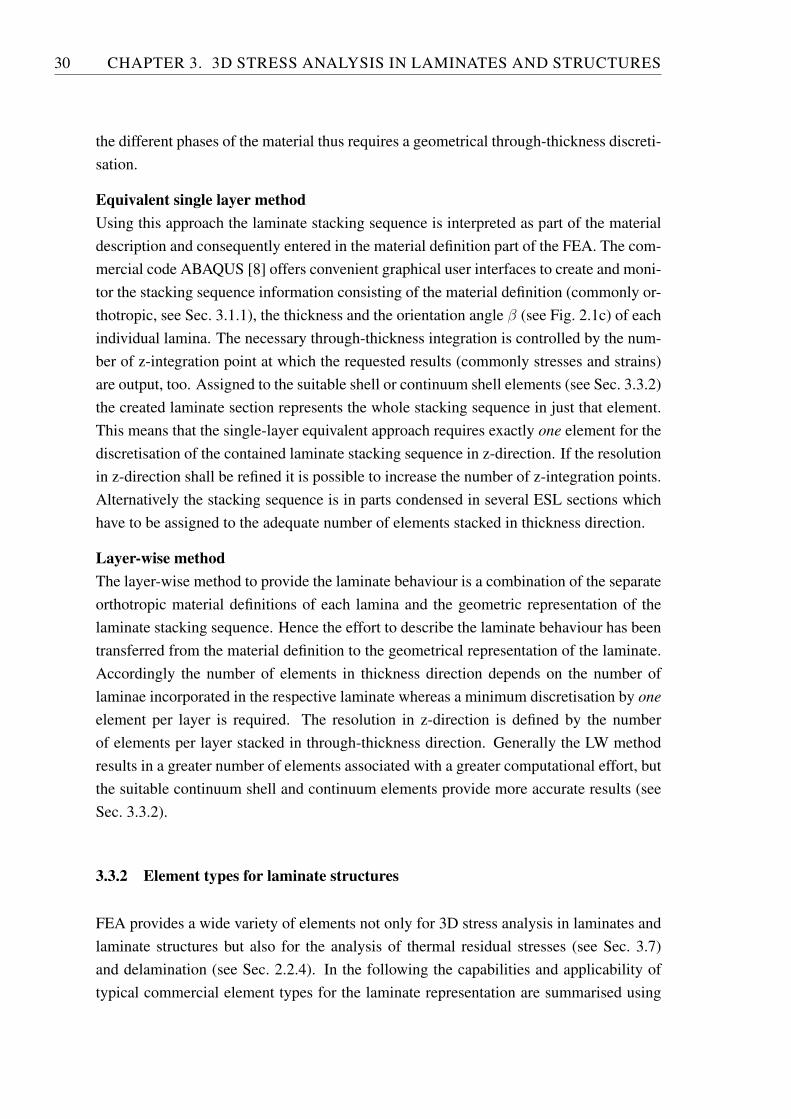
30 CHAPTER 3. 3D STRESS ANALYSIS IN LAMINATES AND STRUCTURES
the different phases of the material thus requires a geometrical through-thickness discreti-sation.
Equivalent single layer methodUsing this approach the laminate stacking sequence is interpreted as part of the materialdescription and consequently entered in the material definition part of the FEA. The com-mercial code ABAQUS [8] offers convenient graphical user interfaces to create and moni-tor the stacking sequence information consisting of the material definition (commonly or-thotropic, see Sec. 3.1.1), the thickness and the orientation angle 𝛽 (see Fig. 2.1c) of eachindividual lamina. The necessary through-thickness integration is controlled by the num-ber of z-integration point at which the requested results (commonly stresses and strains)are output, too. Assigned to the suitable shell or continuum shell elements (see Sec. 3.3.2)the created laminate section represents the whole stacking sequence in just that element.This means that the single-layer equivalent approach requires exactly one element for thediscretisation of the contained laminate stacking sequence in z-direction. If the resolutionin z-direction shall be refined it is possible to increase the number of z-integration points.Alternatively the stacking sequence is in parts condensed in several ESL sections whichhave to be assigned to the adequate number of elements stacked in thickness direction.
Layer-wise methodThe layer-wise method to provide the laminate behaviour is a combination of the separateorthotropic material definitions of each lamina and the geometric representation of thelaminate stacking sequence. Hence the effort to describe the laminate behaviour has beentransferred from the material definition to the geometrical representation of the laminate.Accordingly the number of elements in thickness direction depends on the number oflaminae incorporated in the respective laminate whereas a minimum discretisation by oneelement per layer is required. The resolution in z-direction is defined by the numberof elements per layer stacked in through-thickness direction. Generally the LW methodresults in a greater number of elements associated with a greater computational effort, butthe suitable continuum shell and continuum elements provide more accurate results (seeSec. 3.3.2).
3.3.2 Element types for laminate structures
FEA provides a wide variety of elements not only for 3D stress analysis in laminates andlaminate structures but also for the analysis of thermal residual stresses (see Sec. 3.7)and delamination (see Sec. 2.2.4). In the following the capabilities and applicability oftypical commercial element types for the laminate representation are summarised using
3.3. LAMINATE AND LAMINATE STRUCTURES IN COMMERCIAL FE CODES 31
laminatestructure
laminaterepresentation
mean surfacereduction
fully 3D
geometricalrepresentation
equivalentsingle layer
layer-wise
elementtype
shell continuum shell solid continuum
ux
uy
uz
rx
ry
rz
ux
uy
uz
ux
uy
uz
ex, , ,
, , , ( , )
e g
s s t t ty xy
x y xy xz yz
g gxz yz, ex, , , , ,
, , , , ,
e e g g g
s s s t t ty y xy xz yz
x y y xy xz yz
availablequantities
Figure 3.4: FE modelling strategies for laminate structures.
the example of ABAQUS [8]. All the mentioned elements are also provided including athermo-mechanical coupling for an analysis including residual stresses. The first step inchoosing an appropriate element type is the decision how the local thicknesses of the lam-inate structure shall be represented in the FE model. For the representation of geometrieswith small thicknesses compared to their lateral extension it may be reasonable to reducethe geometry to its mean surface, thus to a flat, locally 2D geometry without a geometricalextension in through-thickness direction. In this case the local thickness of the structureis interpreted as a material parameter. Alternatively the local thickness of the structuremay be retained in the discretised geometry which results in a fully three-dimensionalFE representation of the structure (see Fig. 3.4). This decision regarding the geometricrepresentation of the structure influences the choice of element types described below andthus the suitable material definition method (see Sec. 3.3.1).
Shell elements
The most conventional group of element types associated with the representation of ge-ometries with small thicknesses compared to their lateral extension are shell elements.
32 CHAPTER 3. 3D STRESS ANALYSIS IN LAMINATES AND STRUCTURES
These elements are used to discretise geometries without any expansion in thickness di-rection – i.e. locally two-dimensional. The thickness information of the represented struc-ture goes into the material definition. Shell elements are provided for thin structures basedon the Kirchhoff kinematics as well as for thick structures based on Reissner kinematicsincluding through-thickness shear contributions due to bending deformation [68]. Ap-plied in a 3D modelling space, thin shell elements feature three translatory degrees offreedom 𝑢 = [𝑢𝑥, 𝑢𝑦, 𝑢𝑧] but only two rotatoric 𝑟𝑦 and 𝑟𝑦 from which the inplane straincomponents 𝜖𝑥, 𝜖𝑦 and 𝛾𝑥𝑦 are evaluated. Thick shell elements feature the full set of trans-latory 𝑢 and rotatoric 𝑟 degrees of freedom from which through-thickness the shear strains𝛾𝑥𝑧 and 𝛾𝑦𝑧 are derived additionally. In both cases, only the inplane stress components 𝜎𝑥,𝜎𝑦 and 𝜏𝑥𝑦 are comprised in the governing differential equations, accordingly only thesemeasures are a result of the solution derived by the Principle of Virtual Displacement(PVD). Furthermore ABAQUS provides through-thickness shear stress results 𝜏𝑥𝑧 and 𝜏𝑦𝑧which are postprocessed by means of the equilibrium equations
∂𝜎𝑥∂𝑥
+∂𝜏𝑦𝑥∂𝑦
+∂𝜏𝑧𝑥∂𝑧
= 0
∂𝜏𝑥𝑦∂𝑥
+∂𝜎𝑦∂𝑦
+∂𝜏𝑧𝑦∂𝑧
= 0
∂𝜏𝑥𝑧∂𝑥
+∂𝜏𝑦𝑧∂𝑦
+∂𝜎𝑧∂𝑧
= 0 .
(3.10)
Neither stress 𝜎𝑧 nor strain components 𝜖𝑧 in through-thickness direction are output. Us-ing a shell element any applied boundary condition is related to the mean surface in gen-eral. Only if advanced FEA packages offer the possibility to apply boundary conditionsto the outmost integration points in z-direction the required continuous displacement fieldover the bi-material interfaces (see Tab. 3.2) can be enforced in a stacked shell discreti-sation. If this is not the case, the z-stacking of shell elements for the representation oflaminates and laminate structures is not recommended. This interdicts a layer-wise mate-rial representation as well.
Continuum shell elements
Continuum shell element are generally based on the kinematics and equations of workdefined for conventional shell elements. However they are used to discretise fully 3Dgeometries. They automatically derive the shell thickness information from geometryif the shell normal has been correctly defined by the user. The necessary shell-analogstrain measures are related to the exclusively available translatory degrees of freedomat the eight corner nodes. Continuum shell elements generally provide the same output
3.4. REFERENCE: ANALYTICAL SOLUTION FOLLOWING PAGANO 33
information as conventional shell elements – no stress 𝜎𝑧 and no strain components 𝜖𝑧either – but they have an unlimited z-stacking capability. Accordingly they are availablefor either equivalent single layer or layer-wise laminate descriptions. The laminates z-direction may be discretised by a single continuum shell element comprising an equivalentsingle layer laminate description or by one or more continuum shell elements per layertogether with the orthotropic material descriptions of the respective laminae.
Solid continuum elements
Solid continuum elements are not commonly recommended for the discretisation of ge-ometries with small thicknesses compared to their lateral extension because the accuracyof these groups of elements relies on balanced spatial proportions. In the case of lami-nate structures this requirement eventually results in a lateral discretisation density whichequals at least the lamina thickness. If possible at all this is extremely computationallyexpensive. The representation of a laminate by solid continuum elements is however freeof axiomatic assumptions regarding the displacement, stress or strain field hence the re-sults are expected to converge against the requirements of table 3.2 for a growing numberof elements stacked in z-direction. A further unique feature is the availability of stress 𝜎𝑧and strain components 𝜖𝑧 in through-thickness direction. Aiming on a truly 3D failure andpost-failure analysis (see Chs. 4 and 5) this output is extremely valueable and suggests theuse of solid continuum elements at least for the detailed analysis of generalised laminatebehaviour (see Sec. 3.5).
3.4 Reference: Analytical solution following Pagano
The numerous combinations of laminate material definitions and laminate structure rep-resentations presented above perform significantly different in terms of output quantitiesand their quality. In the following a number of modelling strategies are compared to ananalytical solution for laminates by Pagano [67]. It is derived from layer-wise equilibriumequations (see App. A) and completely fulfils the requirements of table 3.2. It is basedon the complete 3D orthotropic material law and neglects neither of the stress or straincomponents of the full 3D space. However it does not include the Reissner kinematics[68] regarding through-thickness shear components arising from a bending deformation.Hence the Pagano analytical solution is restricted to thin laminate plates. It is valid forrectangular, simply supported laminate plates under an sinusoidal load applied to the top
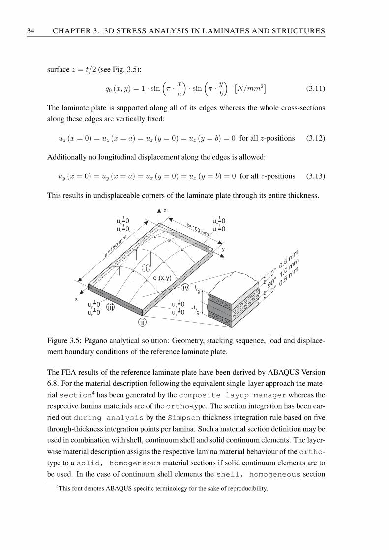
34 CHAPTER 3. 3D STRESS ANALYSIS IN LAMINATES AND STRUCTURES
surface 𝑧 = 𝑡/2 (see Fig. 3.5):
𝑞0 (𝑥, 𝑦) = 1 ⋅ sin(𝜋 ⋅ 𝑥
𝑎
)⋅ sin
(𝜋 ⋅ 𝑦
𝑏
) [𝑁/𝑚𝑚2
](3.11)
The laminate plate is supported along all of its edges whereas the whole cross-sectionsalong these edges are vertically fixed:
𝑢𝑧 (𝑥 = 0) = 𝑢𝑧 (𝑥 = 𝑎) = 𝑢𝑧 (𝑦 = 0) = 𝑢𝑧 (𝑦 = 𝑏) = 0 for all 𝑧-positions (3.12)
Additionally no longitudinal displacement along the edges is allowed:
𝑢𝑦 (𝑥 = 0) = 𝑢𝑦 (𝑥 = 𝑎) = 𝑢𝑥 (𝑦 = 0) = 𝑢𝑥 (𝑦 = 𝑏) = 0 for all 𝑧-positions (3.13)
This results in undisplaceable corners of the laminate plate through its entire thickness.
y
x
z
a=15
0 m
m
b=100 mm
0° 0
.5 m
m
90° 1
.0 m
m
0° 0
.5 m
m
t/2
t- /2
q (x,y)0
u =0
u =0x
z
!
!
u =0
u =0y
z
!
!
u =0
u =0y
z
!
!
u =0
u =0x
z
!
!
iii
i
ii
iv
Figure 3.5: Pagano analytical solution: Geometry, stacking sequence, load and displace-ment boundary conditions of the reference laminate plate.
The FEA results of the reference laminate plate have been derived by ABAQUS Version6.8. For the material description following the equivalent single-layer approach the mate-rial section4 has been generated by the composite layup manager whereas therespective lamina materials are of the ortho-type. The section integration has been car-ried out during analysis by the Simpson thickness integration rule based on fivethrough-thickness integration points per lamina. Such a material section definition may beused in combination with shell, continuum shell and solid continuum elements. The layer-wise material description assigns the respective lamina material behaviour of the ortho-type to a solid, homogeneous material sections if solid continuum elements are tobe used. In the case of continuum shell elements the shell, homogeneous section
4This font denotes ABAQUS-specific terminology for the sake of reproducibility.
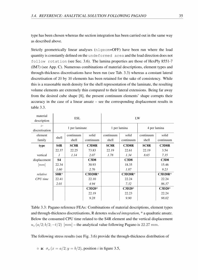
3.4. REFERENCE: ANALYTICAL SOLUTION FOLLOWING PAGANO 35
type has been chosen whereas the section integration has been carried out in the same wayas described above.
Strictly geometrically linear analyses (nlgeom=OFF) have been run where the loadquantity is constantly defined on the undeformed area and the load direction does notfollow rotation (see Sec. 3.6). The lamina properties are those of HexPly 8551-7(IM7) (see App. C). Numerous combinations of material descriptions, element types andthrough-thickness discretisations have been run (see Tab. 3.3) whereas a constant lateraldiscretisation of 20 by 30 elements has been retained for the sake of consistency. Whilethis is a reasonable mesh density for the shell representation of the laminate, the resultingvolume elements are extremely thin compared to their lateral extensions. Being far awayfrom the desired cube shape [8], the present continuum elements’ shape corrupts theiraccuracy in the case of a linear ansatz – see the corresponding displacement results intable 3.3.
materialESL LW
description𝑧-
1 per laminate 1 per lamina 4 per laminadiscretisation
elementshell
continuum solid continuum solid continuum solidfamily shell continuum shell continuum shell continuum
type S4R SC8R C3D8R SC8R C3D8R SC8R C3D8R22.37 22.25 73.83 22.19 22.61 22.19 3.54
vertical 1 1.14 2.07 1.78 1.34 8.65 7.35displacement S4 C3D8 C3D8 C3D8
[𝑚𝑚] 22.34 30.93 18.35 15.461.60 2.76 1.87 9.23
relative S8R* C3D20R* C3D20R* C3D20R*CPU time 22.41 22.10 22.24 22.24
2.01 4.94 7.32 86.37C3D20* C3D20* C3D20*
22.19 22.23 22.249.28 9.90 98.02
Table 3.3: Pagano reference FEAs: Combinations of material descriptions, element typesand through-thickness discretisations, R denotes reduced integration, * a quadratic ansatz.Below the consumed CPU time related to the S4R element and the vertical displacement𝑢𝑧 (𝑎/2; 𝑏/2;−𝑡/2) [𝑚𝑚] – the analytical value following Pagano is 22.27𝑚𝑚.
The following stress results (see Fig. 3.6) provide the through-thickness distribution of
∘ a: 𝜎𝑥 (𝑥 = 𝑎/2; 𝑦 = 𝑏/2), position 𝑖 in figure 3.5,
36 CHAPTER 3. 3D STRESS ANALYSIS IN LAMINATES AND STRUCTURES
∘ b: 𝜎𝑦 (𝑥 = 𝑎/2; 𝑦 = 𝑏/2), position 𝑖 in figure 3.5,
∘ c: 𝜎𝑧 (𝑥 = 𝑎/2; 𝑦 = 𝑏/2), position 𝑖 in figure 3.5,
∘ d: 𝜏𝑥𝑦 (𝑥 = 𝑎; 𝑦 = 𝑏), position 𝑖𝑖 in figure 3.5,
∘ e: 𝜏𝑥𝑧 (𝑥 = 𝑎; 𝑦 = 𝑏/2), position 𝑖𝑖𝑖 in figure 3.5, and
∘ f: 𝜏𝑦𝑧 (𝑥 = 𝑎/2; 𝑦 = 𝑏), position 𝑖𝑣 in figure 3.5
for selected discretisations and element types and compares them to the analytical solu-tion. Looking at these analytical solutions provides a deeper understanding of the through-thickness distributions:
∘ The inplane stresses 𝜎𝑥 and 𝜎𝑦 (see Figs. 3.6a and b) exhibit the expected jumpsover the bi-material interfaces due to the required continuous strain fields. Thestresses in those laminae are higher, which possess the higher stiffness against thecorresponding strain component, i.e. have their fibres oriented in the direction ofthat strain component.
∘ The through-thickness stress 𝜎𝑧 (see Fig. 3.6c) takes the value of the externallyapplied stress on the top surface (𝑧 = 1) and equals 0 on the bottom face (𝑧 = −1)according to the free surface condition.
∘ The inplane shear stress 𝜏𝑥𝑦 is a straight line through the plate’s whole thicknessknown from isotropic material (see Fig. 3.6d). As all layers are made of the samelamina material, they possess an identical stiffness against inplane shear no matterwhat their orientations are.
∘ Despite their different appearance, the distributions of the two through-thicknessshear stresses 𝜏𝑥𝑧 and 𝜏𝑦𝑧 (see Figs. 3.6e and f) differ in quantity only. The generallyshow the same continuous slope and fulfil the free surface condition, i.e. no shearstresses, on the top and bottom of the laminate.
For the comparison between different FEA results figure 3.6 concentrates on four modelrepresentations:
∘ ESL, S4R: An equivalent single layer discretisation (see Sec. 3.2.1) with four-nodelinear shell elements with reduced integration. This model representation is com-putationally extremely cheap and is used for, e.g., complete vehicle simulations.The provided stress results show excellent agreement with the analytical solutions
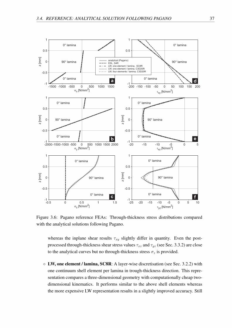
3.4. REFERENCE: ANALYTICAL SOLUTION FOLLOWING PAGANO 37
-1
-0.5
0
0.5
1
-1500 -1000 -500 0 500 1000 1500
sx [N/mm2]
z [
mm
]
-1
-0.5
0
0.5
1
-2000-1500-1000 -500 0 500 1000 1500 2000
z [
mm
]
sy [N/mm2]
-1
-0.5
0
0.5
1
-0.5 0 0.5 1 1.5
z [
mm
]
sz [N/mm2]
-1
-0.5
0
0.5
1
-200 -150 -100 -50 0 50 100 150 200
txy [N/mm2]
-1
-0.5
0
0.5
1
-20 -15 -10 -5 0 5
z [
mm
]
txz [N/mm2]
-1
-0.5
0
0.5
1
-25 -20 -15 -10 -5 0 5 10
z [
mm
]
tyz [N/mm2]
ESL, S4R
LW, one element / lamina, SC8R
LW, one element / lamina, C3D20R
LW, four elements / lamina, C3D20R
analytical (Pagano)
a
c
b e
d
f
0° lamina
0° lamina
90° lamina
0° lamina
0° lamina
90° lamina
0° lamina
0° lamina
90° lamina
0° lamina
0° lamina
90° lamina
0° lamina
0° lamina
90° lamina
0° lamina
0° lamina
90° lamina
Figure 3.6: Pagano reference FEAs: Through-thickness stress distributions comparedwith the analytical solutions following Pagano.
whereas the inplane shear results 𝜏𝑥𝑦 slightly differ in quantity. Even the post-processed through-thickness shear stress values 𝜏𝑥𝑧 and 𝜏𝑦𝑧 (see Sec. 3.3.2) are closeto the analytical curves but no through-thickness stress 𝜎𝑧 is provided.
∘ LW, one element / lamina, SC8R: A layer-wise discretisation (see Sec. 3.2.2) withone continuum shell element per lamina in trough-thickness direction. This repre-sentation compares a three-dimensional geometry with computationally cheap two-dimensional kinematics. It performs similar to the above shell elements whereasthe more expensive LW representation results in a slightly improved accuracy. Still
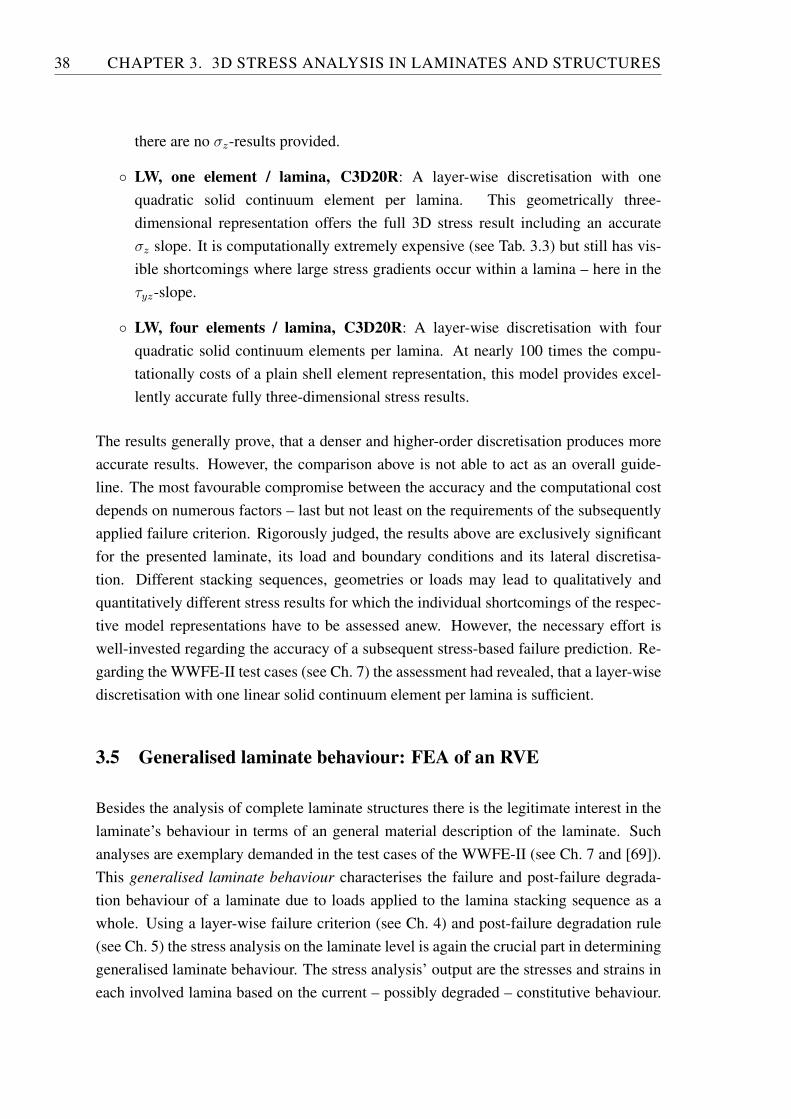
38 CHAPTER 3. 3D STRESS ANALYSIS IN LAMINATES AND STRUCTURES
there are no 𝜎𝑧-results provided.
∘ LW, one element / lamina, C3D20R: A layer-wise discretisation with onequadratic solid continuum element per lamina. This geometrically three-dimensional representation offers the full 3D stress result including an accurate𝜎𝑧 slope. It is computationally extremely expensive (see Tab. 3.3) but still has vis-ible shortcomings where large stress gradients occur within a lamina – here in the𝜏𝑦𝑧-slope.
∘ LW, four elements / lamina, C3D20R: A layer-wise discretisation with fourquadratic solid continuum elements per lamina. At nearly 100 times the compu-tationally costs of a plain shell element representation, this model provides excel-lently accurate fully three-dimensional stress results.
The results generally prove, that a denser and higher-order discretisation produces moreaccurate results. However, the comparison above is not able to act as an overall guide-line. The most favourable compromise between the accuracy and the computational costdepends on numerous factors – last but not least on the requirements of the subsequentlyapplied failure criterion. Rigorously judged, the results above are exclusively significantfor the presented laminate, its load and boundary conditions and its lateral discretisa-tion. Different stacking sequences, geometries or loads may lead to qualitatively andquantitatively different stress results for which the individual shortcomings of the respec-tive model representations have to be assessed anew. However, the necessary effort iswell-invested regarding the accuracy of a subsequent stress-based failure prediction. Re-garding the WWFE-II test cases (see Ch. 7) the assessment had revealed, that a layer-wisediscretisation with one linear solid continuum element per lamina is sufficient.
3.5 Generalised laminate behaviour: FEA of an RVE
Besides the analysis of complete laminate structures there is the legitimate interest in thelaminate’s behaviour in terms of an general material description of the laminate. Suchanalyses are exemplary demanded in the test cases of the WWFE-II (see Ch. 7 and [69]).This generalised laminate behaviour characterises the failure and post-failure degrada-tion behaviour of a laminate due to loads applied to the lamina stacking sequence as awhole. Using a layer-wise failure criterion (see Ch. 4) and post-failure degradation rule(see Ch. 5) the stress analysis on the laminate level is again the crucial part in determininggeneralised laminate behaviour. The stress analysis’ output are the stresses and strains ineach involved lamina based on the current – possibly degraded – constitutive behaviour.
3.5. GENERALISED LAMINATE BEHAVIOUR: FEA OF AN RVE 39
The procedure described below is intended to determine a general material behaviourwhich is independent from the laminate’s inplane dimensions. Accordingly in an appro-priate stress analysis on the laminate level the laminate’s dimension in x- and y-directionmay only play a limited role as auxiliary quantities.
While analytical algorithms like Classical Laminate Theory (CLT) are most efficientlyused for the prediction of inplane behaviour [70–73], 3D load cases clearly exceed theirapplicability. Though there are analytical approaches to the 3D-stress analysis of lami-nates, closed form solutions are only known for few specific cases of rectangular laminatesunder sinusoidal transverse load (see Sec. 3.4 and [67]). Alternatively the RepresentativeVolume Element (RVE) or unit cell approach currently gains more and more importancein the numerical determination of generalised material behaviour of multiphase materials[74, 75]. The basic idea behind RVEs is that the elastic energy stored inside a unit cell isidentical to the one stored inside the represented homogenised continuum. The RVE is avolume that is microstructurally typical of the material system. Therefore, it must containan adequate number of the different material phases, inclusions, defects, voids or cracks.In principle, the inner structure of a unit cell is arbitrary, structured or not, but with therequirement to replicate periodically in space. The method is capable of modelling thematerial behaviour of multi-phase composites, cellular solids or multi-dissipative materi-als, e.g., as long as homogenisation is permitted [16].
Within the desired representation the determined behaviour of the material should notdepend on the dimension of the analysed material section, accordingly the determinedgeneral material behaviour is called statistically homogeneous [18–20]. The smallest vol-ume where this condition applies defines the Representative Volume Element (RVE) orunit cell. By definition an RVE is microscopically large enough to include the relevantinhomogeneities and macroscopically small enough to be regarded as a single materialpoint. The behaviour of the unit cell represents the average response of the material tothe applied loading. This average in form of a macroscopic stress-strain state can be cal-culated in various manners. Efficient analytical solutions are available for simple caseswith respect to geometry, material behaviour and loading conditions [14, 15]. SimpleRVEs can be combined to build up more complex microstructures. This procedure callsfor a combination of analytical and numerical solutions – the generalised method of cells(GMC). The Structures and Acoustics Division of the NASA implemented this techniqueto provide a micromechanical analysis tool [17]. Increasing computational power weak-ened the need for analytical solutions, and ab-initio numerical solutions for unit cellsbecame computationally affordable. Since FEA is the standard tool for the structuralanalysis, its application to the RVE computation is straightforward. Numerical solutiontechniques entail the advantages to include geometric (see Sec. 3.6) and material nonlin-
40 CHAPTER 3. 3D STRESS ANALYSIS IN LAMINATES AND STRUCTURES
earities (see Sec. 3.1.2) as well as complex interface, boundary and loading conditions.Complex non-continuous structures can be represented in a much more refined way aswell (see Fig. 5.7).
Whereas FEA is a common tool for the stress analysis on the structural level, the determi-nation of general material behaviour of a laminate or a non-continuous (see Sec. 5.6) ornon-homogeneous structure [76] is a field of application which requires further consider-ations. The abstract aim is the determination of the general behaviour of a volume (herethe RVE) independent from interfering effects of clamping or load induction. By defini-tion an RVE has to contain all the material inhomogeneities in a representative manner.Transferring this requirement to a laminate, the material inhomogeneities consist of thedifferent laminae and their stacking sequence in z-direction only (see Fig. 3.7) and theRVEs inplane dimensions are arbitrary. The x-z- and y-z-faces have to fulfil the periodic-ity requirement whereas the x-y-faces (top and bottom) are except from this because theseRVE faces represent free surfaces of the material.
x
yz
A
Breference
point
PA
PB
referencepoint
uB
uPB
uPA
uA
Figure 3.7: FE model: RVE representation of the laminate including exemplary x-displacement constraints for two opposed nodes.
Periodic boundary conditions are not commonly implemented in commercial FEA pack-ages. The requirement that a deformed or undeformed RVE has to allow its periodicallyassembly to an endless row in any coordinate direction results in the requirement of equaltopography of opposed faces. This is achieved by the introduction of one additional ref-erence point per face [77]. The approach is exemplary shown in figure 3.7 for the twoy-z-faces of the RVE. The two reference points 𝑃𝐴 and 𝑃𝐵 are allowed to move in orderto enable an overall normal or shear deformation of the RVE. However the relative dis-placement between an arbitrary node on the surface 𝐴 and its reference point 𝑃𝐴 is setequal to the relative displacement between the respective partner node on the opposite
3.6. GEOMETRIC NONLINEARITY 41
surface 𝐵 and its reference point 𝑃𝐵:
𝑢𝐴 − 𝑢𝑃𝐴= 𝑢𝐵 − 𝑢𝑃𝐵
(3.14)
This procedure ensures that the deformation of face 𝐴 is equal to the one of face 𝐵whereas the two faces are still allowed the relative motion between each other. The ap-proach requires an equal FE mesh on opposed faces and may result in a large number ofdisplacement constraints in the case of complex geometries (see Sec. 5.6). Earlier appli-cations of the developed approach [78] revealed that the periodicity requirement not onlyrefers to displacements but to stresses as well. Analysing unsymmetric RVE geometriesor loads the stress periodicity is not achieved by the measures described above. The def-inition of stress boundary conditions however requires finite elements with mixed stress-strain-formulations [46] which are currently not available in commercial FEA packages.
Regarding the discretisation of the laminate RVE the FE model needs no discretisationalong the two inplane directions due to the RVE’s arbitrary inplane dimensions. Neglect-ing bending load cases and unsymmetric laminates, there are only homogeneous statesof stress throughout the lamina’s thickness direction expected. Thus only one elementper lamina is sufficient for the WWFE-II load cases (see Fig. 3.7). Though commercialFE packages offer various shell elements for the representation of laminates and laminatestructures (see Sec. 3.3.2), their 3D capabilities in terms of stress results are still limited(see Sec. 3.4). Thus the RVE model applied to the WWFE-II test cases (see Ch. 7) usesfully integrated linear volume elements.
3.6 Geometric nonlinearity
UD FRC laminae are highly orthotropic materials with considerably different constitutivebehaviour in the respective directions. When subjected to a load the material’s reactiondepends on its orientation towards that load. In the case of UD FRCs very little variancesin the orientation may have significant effects – particularly in the case of fibre-parallelapplied load. Increasingly loaded the material’s orientation might change during the pro-cess and therewith changes its orientation towards and its reaction due to this appliedload.
A static Finite Element Analysis offers two ways of forming the equilibrium - geomet-rically linear based on the original geometry or nonlinear based on the actual geometry.The reasons above highly recommend to run geometrically nonlinear analyses when pre-dicting UD FRC’s failure and post-failure behaviour, particularly in the case of largedeformations above 5% or in shear load cases. This approach automatically includes the
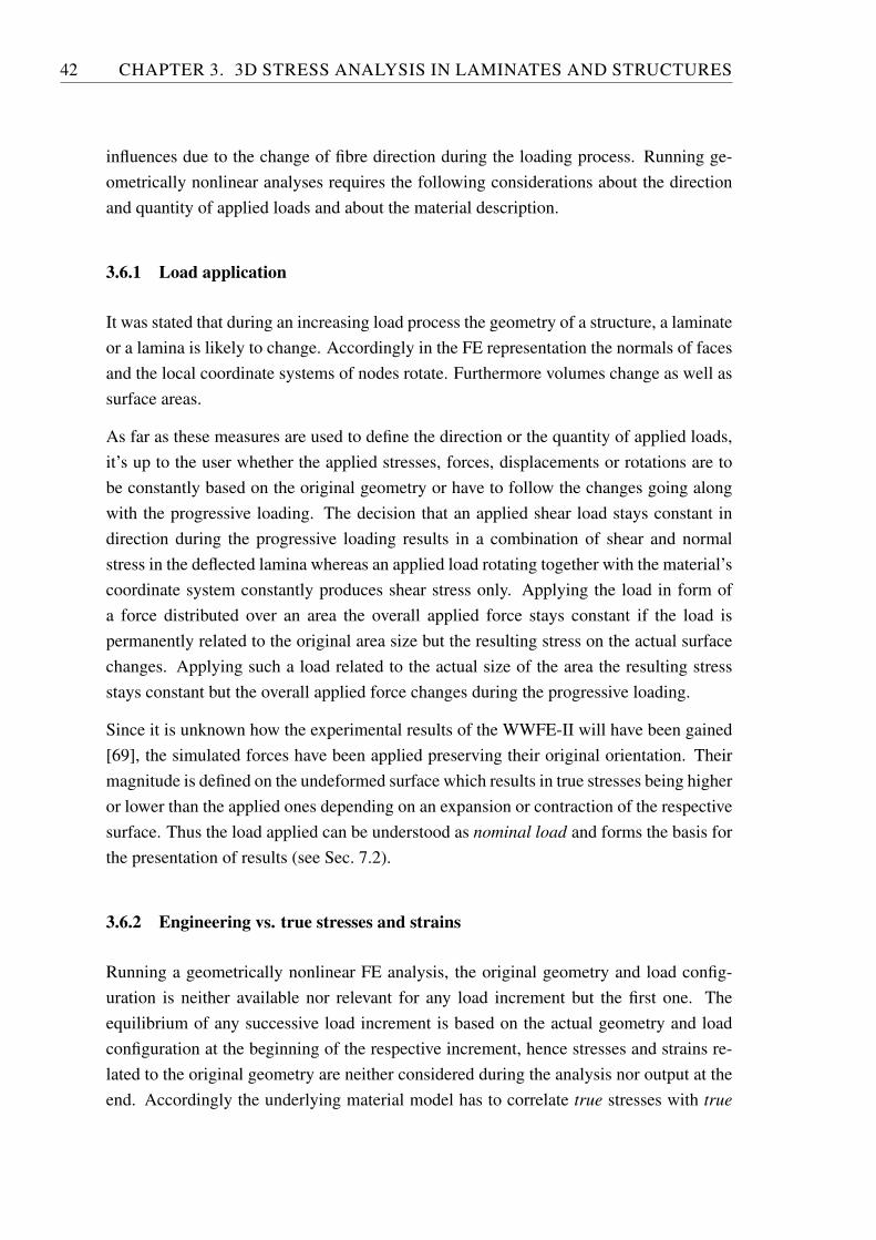
42 CHAPTER 3. 3D STRESS ANALYSIS IN LAMINATES AND STRUCTURES
influences due to the change of fibre direction during the loading process. Running ge-ometrically nonlinear analyses requires the following considerations about the directionand quantity of applied loads and about the material description.
3.6.1 Load application
It was stated that during an increasing load process the geometry of a structure, a laminateor a lamina is likely to change. Accordingly in the FE representation the normals of facesand the local coordinate systems of nodes rotate. Furthermore volumes change as well assurface areas.
As far as these measures are used to define the direction or the quantity of applied loads,it’s up to the user whether the applied stresses, forces, displacements or rotations are tobe constantly based on the original geometry or have to follow the changes going alongwith the progressive loading. The decision that an applied shear load stays constant indirection during the progressive loading results in a combination of shear and normalstress in the deflected lamina whereas an applied load rotating together with the material’scoordinate system constantly produces shear stress only. Applying the load in form ofa force distributed over an area the overall applied force stays constant if the load ispermanently related to the original area size but the resulting stress on the actual surfacechanges. Applying such a load related to the actual size of the area the resulting stressstays constant but the overall applied force changes during the progressive loading.
Since it is unknown how the experimental results of the WWFE-II will have been gained[69], the simulated forces have been applied preserving their original orientation. Theirmagnitude is defined on the undeformed surface which results in true stresses being higheror lower than the applied ones depending on an expansion or contraction of the respectivesurface. Thus the load applied can be understood as nominal load and forms the basis forthe presentation of results (see Sec. 7.2).
3.6.2 Engineering vs. true stresses and strains
Running a geometrically nonlinear FE analysis, the original geometry and load config-uration is neither available nor relevant for any load increment but the first one. Theequilibrium of any successive load increment is based on the actual geometry and loadconfiguration at the beginning of the respective increment, hence stresses and strains re-lated to the original geometry are neither considered during the analysis nor output at theend. Accordingly the underlying material model has to correlate true stresses with true
3.6. GEOMETRIC NONLINEARITY 43
strains rather than engineering values as they are commonly determined in experiments.Whereas engineering stresses are the quotient of the force 𝐹 and the original cross-section
F
A0 A
x
yz
a0
b0
a b
F
F+ FD
Dl(F)
D Dl( F)
l0
l
Figure 3.8: Change of material’s cross-section area (a) and length (b) due to an uniaxiallyapplied tensile load 𝐹 .
area 𝐴0 (see Fig. 3.8a), the true stress is derived by using the deformed cross-section area𝐴 (𝐹 ):
𝜎𝑒𝑛𝑔𝑖𝑛 =𝐹
𝐴0
and 𝜎𝑡𝑟𝑢𝑒 =𝐹
𝐴 (𝐹 )=
𝐹
𝐴 (𝜖𝑥)=
𝐹
𝑎 (𝜖𝑥) ⋅ 𝑏 (𝜖𝑥) (3.15)
The strain in x-direction 𝜖𝑥 induces the two lateral contractions
𝜖𝑦 = −𝜈𝑥𝑦 ⋅ 𝜖𝑥 and 𝜖𝑧 = −𝜈𝑥𝑧 ⋅ 𝜖𝑥 (3.16)
whereas the quantitative effects on the dimensions are
𝑎 = 𝑎0 ⋅ (1 + 𝜖𝑦) and 𝑏 = 𝑏0 ⋅ (1 + 𝜖𝑧) . (3.17)
From equations 3.15 to 3.17 the relation between true and engineering stress is
𝜎𝑡𝑟𝑢𝑒 =𝜎𝑒𝑛𝑔𝑖𝑛
1− (𝜈𝑥𝑦 + 𝜈𝑥𝑧) ⋅ 𝜖𝑥 + 𝜈𝑥𝑦 ⋅ 𝜈𝑥𝑧 ⋅ 𝜖2𝑥. (3.18)
Note that equation 3.18 differs from the commonly cited Ludwik law 𝜎𝑡𝑟𝑢𝑒 = 𝜎𝑒𝑛𝑔𝑖𝑛 ⋅(1 + 𝜖𝑥) which postulates a costant volume [79]. This relation is valid for fully plasticdeformation only, thus is not relevant here.
An analogous consideration relates true and engineering strains by means of figure 3.8bwhere a load increase by Δ𝐹 results in an additional elongation Δ𝑙 (Δ𝐹 ):
Δ𝜖𝑒𝑛𝑔𝑖𝑛 =Δ𝑙 (Δ𝐹 )
𝑙0and Δ𝜖𝑡𝑟𝑢𝑒 =
Δ𝑙 (Δ𝐹 )
𝑙 (𝐹 )=
Δ𝑙 (Δ𝐹 )
𝑙0 +Δ𝑙 (𝐹 )(3.19)
Integrating from 𝑙0 to a deformed 𝑙 represents a summation of infinitesimally small loadincrements [80] and the result is
𝜖𝑡𝑟𝑢𝑒 = ln
(𝑙
𝑙0
)in contrast to 𝜖𝑒𝑛𝑔𝑖𝑛 =
𝑙 − 𝑙0𝑙0
. (3.20)
Equation 3.20 points out why true strains are often referred to by the term logarithmicstrains.
44 CHAPTER 3. 3D STRESS ANALYSIS IN LAMINATES AND STRUCTURES
3.7 Residual stresses
UD fibre reinforced laminae show orthotropic behaviour in terms of thermal expansion.In the process of curing a laminate, this leads to residual stresses in the final laminate. Theprocess is chemically and thermodynamically challenging. Influences like tempering his-tory, ambient pressure and humidity are hardly to cover in a structural mechanics context.However the representation of the process by a simple cooling from stress free temper-ature to room temperature using linear thermal coefficients is intuitive but overestimatesthe resulting residual stresses according to our experience [5, 6]. Puck assumes the trueresidual stresses to reach half the values calculated from this approach. Accordingly thepresented analyses are based on half the temperature drop from the stress free temperatureto ambient temperature (see Sec. 7.2).
Including thermal expansion within a thermo-mechanically coupled analysis is a standardprocedure in contemporary commercial FE packages and is carried out independentlyfrom Puck’s Theory contained in the user-defined material description (see Ch. 6). Notethat in the case of FEA, the thermally induced residual stresses are automatically subjectto the nonlinear constitutive behaviour of the material. In contrast to most analytical ap-proaches, the residual stresses are not calculated at first and then constantly superposedbut they are incrementally computed from the residual strains and the current secant stiff-ness.
4 Puck’s failure theory
The present chapter concentrates on the fracture criteria for unidirectionally fibre rein-forced polymer composites (UD FRPCs) developed by Puck. As the first World-WideFailure Exercise [2] encyclopedically compares currently available failure criteria, thepresent work does not compare Puck’s criteria with competitive approaches. After a shortintroduction to failure hypothesis in general (see Sec. 4.1), the chapter describes Puck’sinter-fibre fracture criterion (see Sec. 4.2) and the associated extensions beyond Mohr’shypothesis (see Sec. 4.3). Before the fibre fracture is addressed in section 4.7, the appli-cation within a laminate (see Sec. 4.5) and to special cases (see Sec. 4.6) is discussed.
4.1 Introduction to failure prediction
The task of a failure criterion is the determination whether an arbitrary load applied tothe lamina leads to a fracture or not. This is commonly achieved by a fracture hypothesiswhich comprehends the set of all possible states of fracture. It is important to understandthe fracture conditions as hypothetical in the sense that they give statements regardingan infinite number of states on the basis of very few known states of fracture. Theseknown – i.e. experimentally accessible, hence determinable states of fracture are referredto as basic strengths. In the case of UD FRCs these are the fractures due to appliedfibre-parallel or fibre-perpendicular tension and compression (𝑅𝑡
∥, 𝑅𝑐∥ , 𝑅𝑡
⊥ and 𝑅𝑐⊥) and
due to inplane and out-of-plane shear (𝑅⊥∥ and 𝑅⊥⊥). These basic strengths may beexpressed in terms of stress or strain, but as Puck’s criteria are stress-based [21] no strainthresholds are considered within this work. The fracture criterion defines a closed surfacein the six-dimensional stress space (𝜎1, 𝜎2, 𝜎3, 𝜏12, 𝜏13, 𝜏23), includes – in the best case –all the available experimental determined strengths and predicts reasonable fractures atall other stress combinations (see Fig. 4.1). This task in mind it becomes evident that afracture criterion can never be more than an hypothesis – i.e. a model representation –of what happens in cases which are not experimentally proven. As an hypothesis fracturecriteria may be proven or contradicted by further experimental results if the criterion is notversatile enough to be adapted to the later findings. The hypothesis may be based on puremathematical considerations regarding a surface-definition or on fracture-mechanical orphysical considerations. The rising number of experimental results has however pointedout the advantage of physically-based fracture conditions of which Puck’s Theory is the
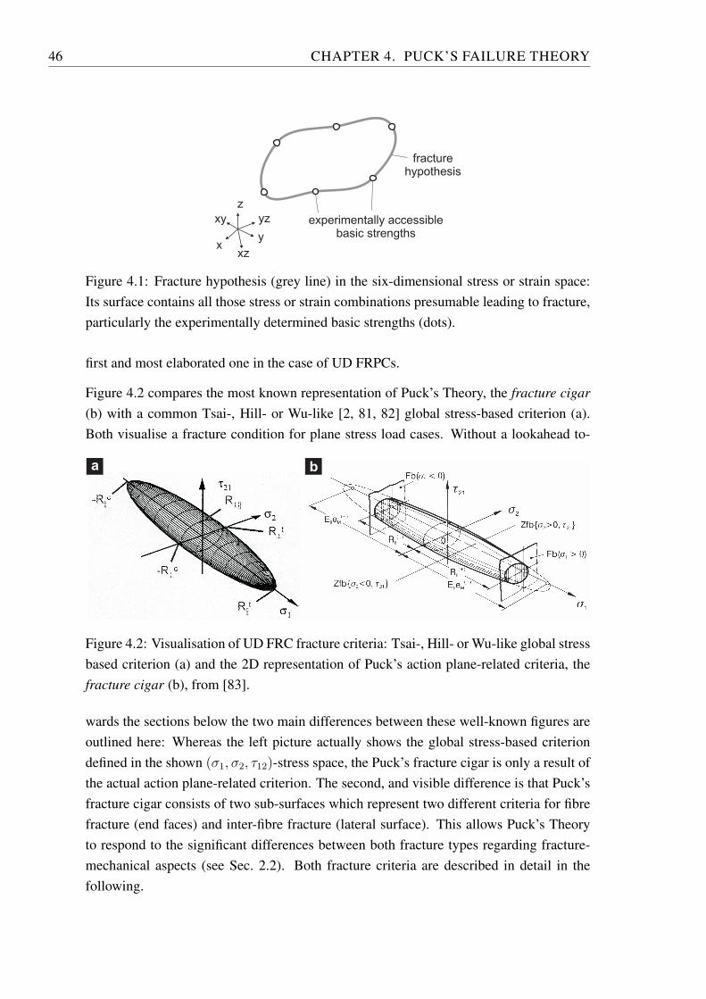
46 CHAPTER 4. PUCK’S FAILURE THEORY
xy
z
xy yz
xz
experimentally accessiblebasic strengths
fracturehypothesis
Figure 4.1: Fracture hypothesis (grey line) in the six-dimensional stress or strain space:Its surface contains all those stress or strain combinations presumable leading to fracture,particularly the experimentally determined basic strengths (dots).
first and most elaborated one in the case of UD FRPCs.
Figure 4.2 compares the most known representation of Puck’s Theory, the fracture cigar(b) with a common Tsai-, Hill- or Wu-like [2, 81, 82] global stress-based criterion (a).Both visualise a fracture condition for plane stress load cases. Without a lookahead to-
ba
Figure 4.2: Visualisation of UD FRC fracture criteria: Tsai-, Hill- or Wu-like global stressbased criterion (a) and the 2D representation of Puck’s action plane-related criteria, thefracture cigar (b), from [83].
wards the sections below the two main differences between these well-known figures areoutlined here: Whereas the left picture actually shows the global stress-based criteriondefined in the shown (𝜎1, 𝜎2, 𝜏12)-stress space, the Puck’s fracture cigar is only a result ofthe actual action plane-related criterion. The second, and visible difference is that Puck’sfracture cigar consists of two sub-surfaces which represent two different criteria for fibrefracture (end faces) and inter-fibre fracture (lateral surface). This allows Puck’s Theoryto respond to the significant differences between both fracture types regarding fracture-mechanical aspects (see Sec. 2.2). Both fracture criteria are described in detail in thefollowing.
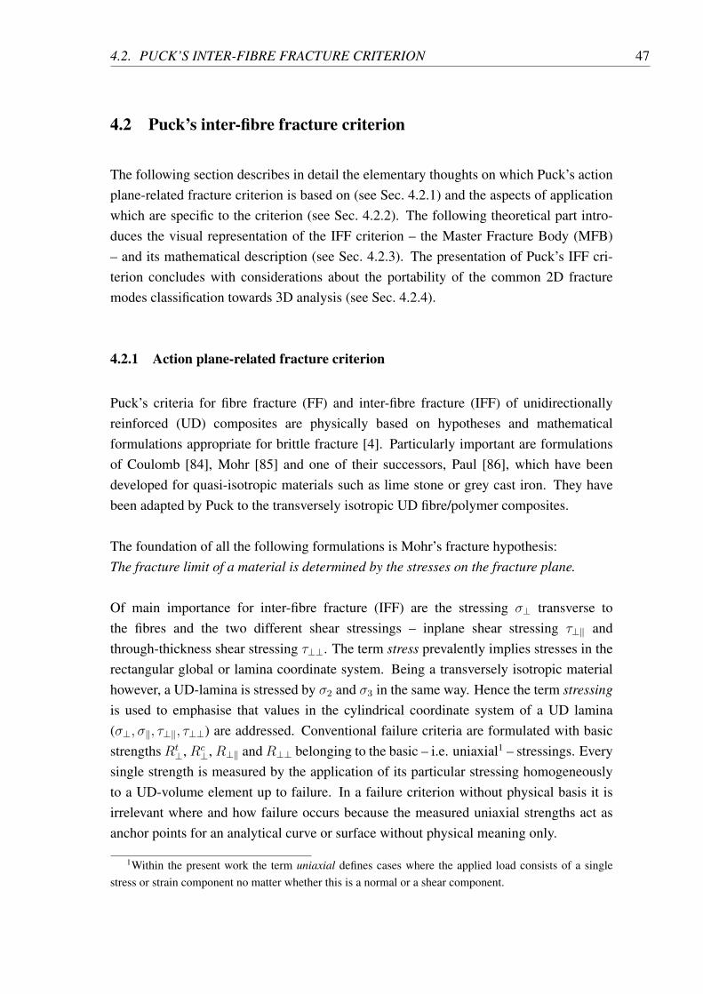
4.2. PUCK’S INTER-FIBRE FRACTURE CRITERION 47
4.2 Puck’s inter-fibre fracture criterion
The following section describes in detail the elementary thoughts on which Puck’s actionplane-related fracture criterion is based on (see Sec. 4.2.1) and the aspects of applicationwhich are specific to the criterion (see Sec. 4.2.2). The following theoretical part intro-duces the visual representation of the IFF criterion – the Master Fracture Body (MFB)– and its mathematical description (see Sec. 4.2.3). The presentation of Puck’s IFF cri-terion concludes with considerations about the portability of the common 2D fracturemodes classification towards 3D analysis (see Sec. 4.2.4).
4.2.1 Action plane-related fracture criterion
Puck’s criteria for fibre fracture (FF) and inter-fibre fracture (IFF) of unidirectionallyreinforced (UD) composites are physically based on hypotheses and mathematicalformulations appropriate for brittle fracture [4]. Particularly important are formulationsof Coulomb [84], Mohr [85] and one of their successors, Paul [86], which have beendeveloped for quasi-isotropic materials such as lime stone or grey cast iron. They havebeen adapted by Puck to the transversely isotropic UD fibre/polymer composites.
The foundation of all the following formulations is Mohr’s fracture hypothesis:The fracture limit of a material is determined by the stresses on the fracture plane.
Of main importance for inter-fibre fracture (IFF) are the stressing 𝜎⊥ transverse tothe fibres and the two different shear stressings – inplane shear stressing 𝜏⊥∥ andthrough-thickness shear stressing 𝜏⊥⊥. The term stress prevalently implies stresses in therectangular global or lamina coordinate system. Being a transversely isotropic materialhowever, a UD-lamina is stressed by 𝜎2 and 𝜎3 in the same way. Hence the term stressingis used to emphasise that values in the cylindrical coordinate system of a UD lamina(𝜎⊥, 𝜎∥, 𝜏⊥∥, 𝜏⊥⊥) are addressed. Conventional failure criteria are formulated with basicstrengths𝑅𝑡
⊥,𝑅𝑐⊥,𝑅⊥∥ and𝑅⊥⊥ belonging to the basic – i.e. uniaxial1 – stressings. Every
single strength is measured by the application of its particular stressing homogeneouslyto a UD-volume element up to failure. In a failure criterion without physical basis it isirrelevant where and how failure occurs because the measured uniaxial strengths act asanchor points for an analytical curve or surface without physical meaning only.
1Within the present work the term uniaxial defines cases where the applied load consists of a singlestress or strain component no matter whether this is a normal or a shear component.
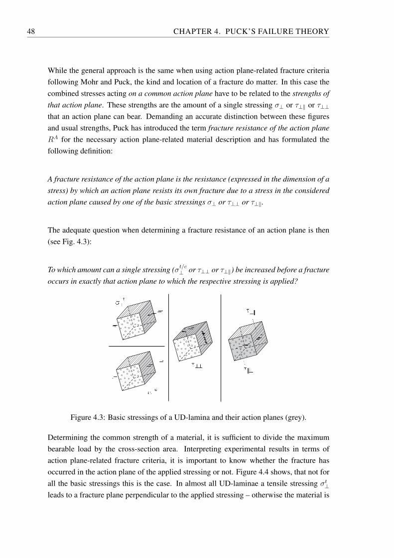
48 CHAPTER 4. PUCK’S FAILURE THEORY
While the general approach is the same when using action plane-related fracture criteriafollowing Mohr and Puck, the kind and location of a fracture do matter. In this case thecombined stresses acting on a common action plane have to be related to the strengths ofthat action plane. These strengths are the amount of a single stressing 𝜎⊥ or 𝜏⊥∥ or 𝜏⊥⊥that an action plane can bear. Demanding an accurate distinction between these figuresand usual strengths, Puck has introduced the term fracture resistance of the action plane𝑅𝐴 for the necessary action plane-related material description and has formulated thefollowing definition:
A fracture resistance of the action plane is the resistance (expressed in the dimension of astress) by which an action plane resists its own fracture due to a stress in the consideredaction plane caused by one of the basic stressings 𝜎⊥ or 𝜏⊥⊥ or 𝜏⊥∥.
The adequate question when determining a fracture resistance of an action plane is then(see Fig. 4.3):
To which amount can a single stressing (𝜎𝑡/𝑐⊥ or 𝜏⊥⊥ or 𝜏⊥∥) be increased before a fractureoccurs in exactly that action plane to which the respective stressing is applied?
Figure 4.3: Basic stressings of a UD-lamina and their action planes (grey).
Determining the common strength of a material, it is sufficient to divide the maximumbearable load by the cross-section area. Interpreting experimental results in terms ofaction plane-related fracture criteria, it is important to know whether the fracture hasoccurred in the action plane of the applied stressing or not. Figure 4.4 shows, that not forall the basic stressings this is the case. In almost all UD-laminae a tensile stressing 𝜎𝑡⊥leads to a fracture plane perpendicular to the applied stressing – otherwise the material is
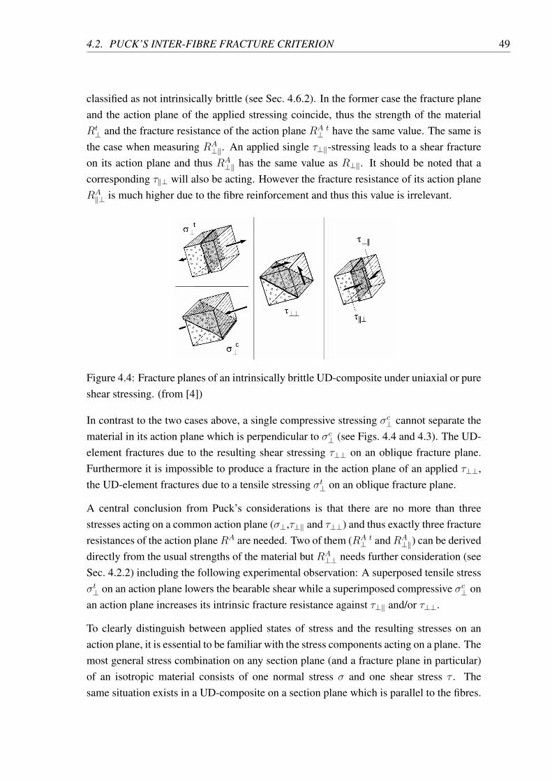
4.2. PUCK’S INTER-FIBRE FRACTURE CRITERION 49
classified as not intrinsically brittle (see Sec. 4.6.2). In the former case the fracture planeand the action plane of the applied stressing coincide, thus the strength of the material𝑅𝑡
⊥ and the fracture resistance of the action plane 𝑅𝐴 𝑡⊥ have the same value. The same is
the case when measuring 𝑅𝐴⊥∥. An applied single 𝜏⊥∥-stressing leads to a shear fracture
on its action plane and thus 𝑅𝐴⊥∥ has the same value as 𝑅⊥∥. It should be noted that a
corresponding 𝜏∥⊥ will also be acting. However the fracture resistance of its action plane𝑅𝐴
∥⊥ is much higher due to the fibre reinforcement and thus this value is irrelevant.
Figure 4.4: Fracture planes of an intrinsically brittle UD-composite under uniaxial or pureshear stressing. (from [4])
In contrast to the two cases above, a single compressive stressing 𝜎𝑐⊥ cannot separate thematerial in its action plane which is perpendicular to 𝜎𝑐⊥ (see Figs. 4.4 and 4.3). The UD-element fractures due to the resulting shear stressing 𝜏⊥⊥ on an oblique fracture plane.Furthermore it is impossible to produce a fracture in the action plane of an applied 𝜏⊥⊥,the UD-element fractures due to a tensile stressing 𝜎𝑡⊥ on an oblique fracture plane.
A central conclusion from Puck’s considerations is that there are no more than threestresses acting on a common action plane (𝜎⊥,𝜏⊥∥ and 𝜏⊥⊥) and thus exactly three fractureresistances of the action plane𝑅𝐴 are needed. Two of them (𝑅𝐴 𝑡
⊥ and𝑅𝐴⊥∥) can be derived
directly from the usual strengths of the material but 𝑅𝐴⊥⊥ needs further consideration (see
Sec. 4.2.2) including the following experimental observation: A superposed tensile stress𝜎𝑡⊥ on an action plane lowers the bearable shear while a superimposed compressive 𝜎𝑐⊥ onan action plane increases its intrinsic fracture resistance against 𝜏⊥∥ and/or 𝜏⊥⊥.
To clearly distinguish between applied states of stress and the resulting stresses on anaction plane, it is essential to be familiar with the stress components acting on a plane. Themost general stress combination on any section plane (and a fracture plane in particular)of an isotropic material consists of one normal stress 𝜎 and one shear stress 𝜏 . Thesame situation exists in a UD-composite on a section plane which is parallel to the fibres.
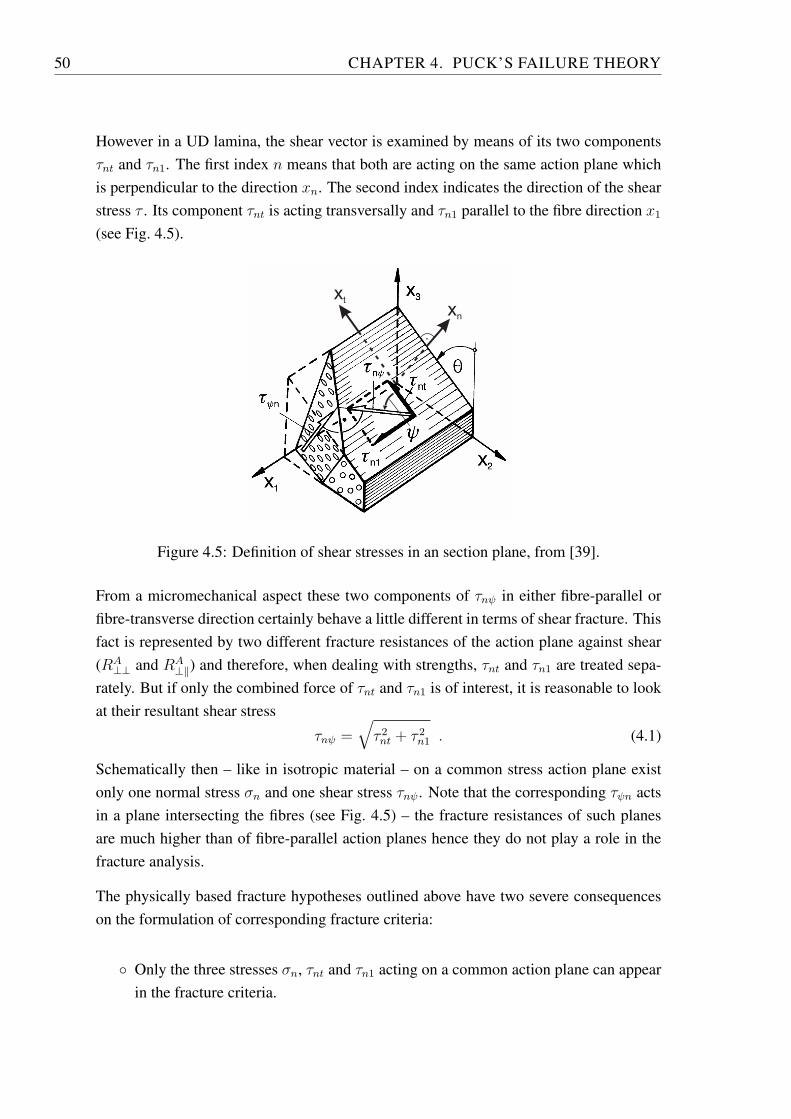
50 CHAPTER 4. PUCK’S FAILURE THEORY
However in a UD lamina, the shear vector is examined by means of its two components𝜏𝑛𝑡 and 𝜏𝑛1. The first index 𝑛 means that both are acting on the same action plane whichis perpendicular to the direction 𝑥𝑛. The second index indicates the direction of the shearstress 𝜏 . Its component 𝜏𝑛𝑡 is acting transversally and 𝜏𝑛1 parallel to the fibre direction 𝑥1(see Fig. 4.5).
xt
xn
Figure 4.5: Definition of shear stresses in an section plane, from [39].
From a micromechanical aspect these two components of 𝜏𝑛𝜓 in either fibre-parallel orfibre-transverse direction certainly behave a little different in terms of shear fracture. Thisfact is represented by two different fracture resistances of the action plane against shear(𝑅𝐴
⊥⊥ and 𝑅𝐴⊥∥) and therefore, when dealing with strengths, 𝜏𝑛𝑡 and 𝜏𝑛1 are treated sepa-
rately. But if only the combined force of 𝜏𝑛𝑡 and 𝜏𝑛1 is of interest, it is reasonable to lookat their resultant shear stress
𝜏𝑛𝜓 =√𝜏 2𝑛𝑡 + 𝜏 2𝑛1 . (4.1)
Schematically then – like in isotropic material – on a common stress action plane existonly one normal stress 𝜎𝑛 and one shear stress 𝜏𝑛𝜓. Note that the corresponding 𝜏𝜓𝑛 actsin a plane intersecting the fibres (see Fig. 4.5) – the fracture resistances of such planesare much higher than of fibre-parallel action planes hence they do not play a role in thefracture analysis.
The physically based fracture hypotheses outlined above have two severe consequenceson the formulation of corresponding fracture criteria:
∘ Only the three stresses 𝜎𝑛, 𝜏𝑛𝑡 and 𝜏𝑛1 acting on a common action plane can appearin the fracture criteria.
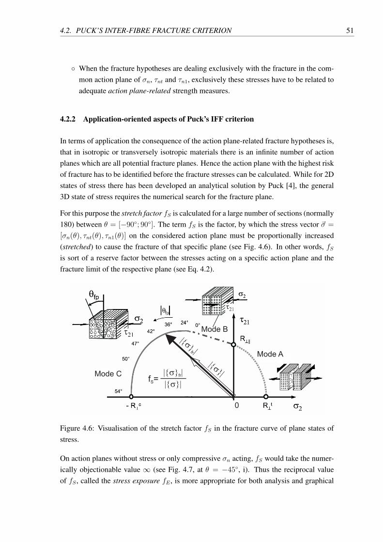
4.2. PUCK’S INTER-FIBRE FRACTURE CRITERION 51
∘ When the fracture hypotheses are dealing exclusively with the fracture in the com-mon action plane of 𝜎𝑛, 𝜏𝑛𝑡 and 𝜏𝑛1, exclusively these stresses have to be related toadequate action plane-related strength measures.
4.2.2 Application-oriented aspects of Puck’s IFF criterion
In terms of application the consequence of the action plane-related fracture hypotheses is,that in isotropic or transversely isotropic materials there is an infinite number of actionplanes which are all potential fracture planes. Hence the action plane with the highest riskof fracture has to be identified before the fracture stresses can be calculated. While for 2Dstates of stress there has been developed an analytical solution by Puck [4], the general3D state of stress requires the numerical search for the fracture plane.
For this purpose the stretch factor 𝑓𝑆 is calculated for a large number of sections (normally180) between 𝜃 = [−90∘; 90∘]. The term 𝑓𝑆 is the factor, by which the stress vector �� =
[𝜎𝑛(𝜃), 𝜏𝑛𝑡(𝜃), 𝜏𝑛1(𝜃)] on the considered action plane must be proportionally increased(stretched) to cause the fracture of that specific plane (see Fig. 4.6). In other words, 𝑓𝑆is sort of a reserve factor between the stresses acting on a specific action plane and thefracture limit of the respective plane (see Eq. 4.2).
f =S
|{s}|fr
|{s}|
|{s} |fr
|{s}|
0
Mode A
Mode B
Mode C
Figure 4.6: Visualisation of the stretch factor 𝑓𝑆 in the fracture curve of plane states ofstress.
On action planes without stress or only compressive 𝜎𝑛 acting, 𝑓𝑆 would take the numer-ically objectionable value ∞ (see Fig. 4.7, at 𝜃 = −45∘, i). Thus the reciprocal valueof 𝑓𝑆 , called the stress exposure 𝑓𝐸 , is more appropriate for both analysis and graphical
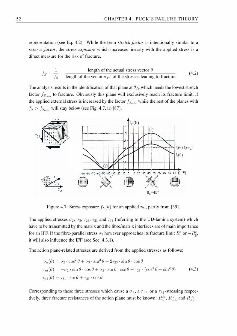
52 CHAPTER 4. PUCK’S FAILURE THEORY
representation (see Eq. 4.2). While the term stretch factor is intentionally similar to areserve factor, the stress exposure which increases linearly with the applied stress is adirect measure for the risk of fracture.
𝑓𝐸 =1
𝑓𝑆=
length of the actual stress vector ��length of the vector ��𝑓𝑟 of the stresses leading to fracture
(4.2)
The analysis results in the identification of that plane at 𝜃𝑓𝑝 which needs the lowest stretchfactor 𝑓𝑆𝑚𝑖𝑛
to fracture. Obviously this plane will exclusively reach its fracture limit, ifthe applied external stress is increased by the factor 𝑓𝑆𝑚𝑖𝑛
while the rest of the planes with𝑓𝑆 > 𝑓𝑆𝑚𝑖𝑛
will stay below (see Fig. 4.7, ii) [87].
i
ii
f ( )E q
f ( )E q ×f ( )S fpq
qfp=45°
1
Figure 4.7: Stress exposure 𝑓𝐸(𝜃) for an applied 𝜏23, partly from [39].
The applied stresses 𝜎2, 𝜎3, 𝜏23, 𝜏21 and 𝜏31 (referring to the UD-lamina system) whichhave to be transmitted by the matrix and the fibre/matrix interfaces are of main importancefor an IFF. If the fibre-parallel stress 𝜎1 however approaches its fracture limit 𝑅𝑡
∥ or −𝑅𝑐∥,
it will also influence the IFF (see Sec. 4.3.1).
The action plane-related stresses are derived from the applied stresses as follows:
𝜎𝑛(𝜃) = 𝜎2 ⋅ cos2 𝜃 + 𝜎3 ⋅ sin2 𝜃 + 2𝜏23 ⋅ sin 𝜃 ⋅ cos 𝜃𝜏𝑛𝑡(𝜃) = −𝜎2 ⋅ sin 𝜃 ⋅ cos 𝜃 + 𝜎3 ⋅ sin 𝜃 ⋅ cos 𝜃 + 𝜏23 ⋅
(cos2 𝜃 − sin2 𝜃
)𝜏𝑛1(𝜃) = 𝜏31 ⋅ sin 𝜃 + 𝜏21 ⋅ cos 𝜃
(4.3)
Corresponding to these three stresses which cause a 𝜎⊥, a 𝜏⊥⊥ or a 𝜏⊥∥-stressing respec-tively, three fracture resistances of the action plane must be known: 𝑅𝐴𝑡
⊥ , 𝑅 𝐴⊥⊥ and 𝑅 𝐴
⊥∥.
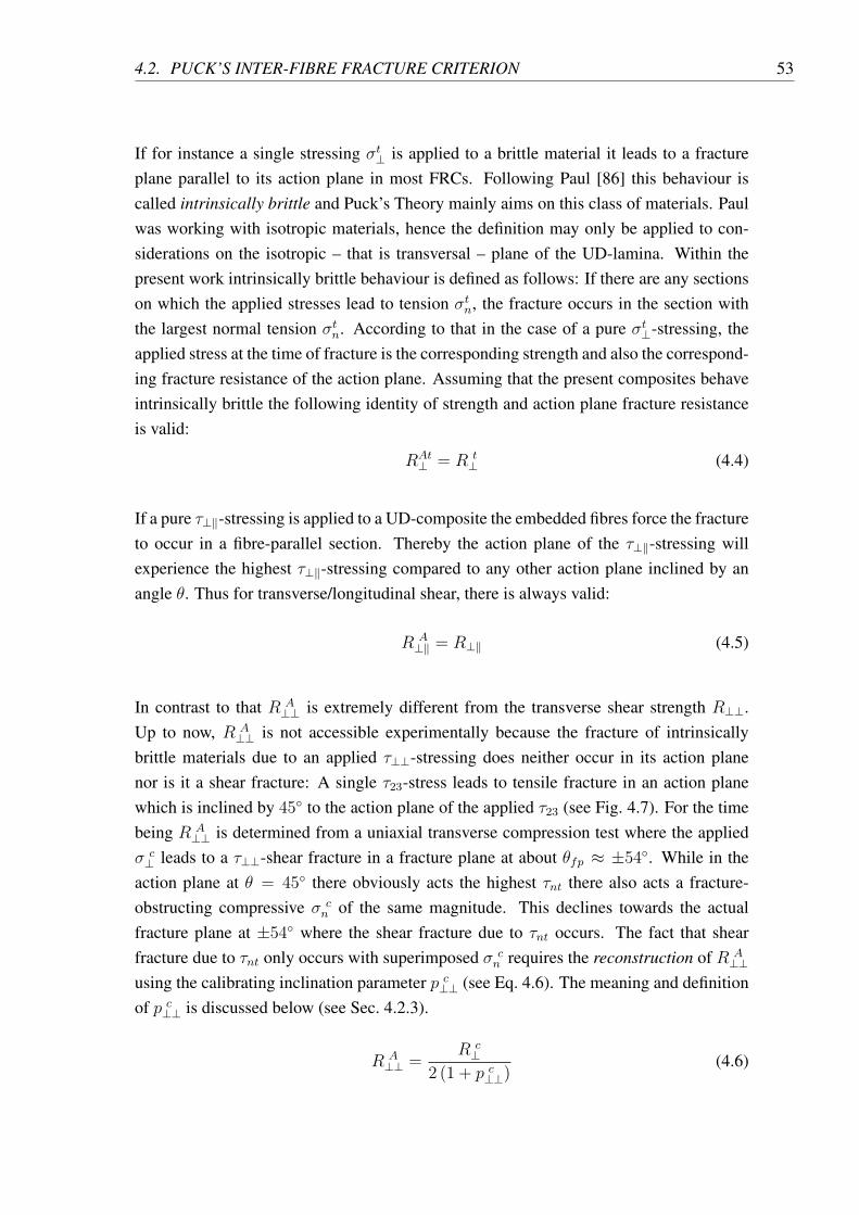
4.2. PUCK’S INTER-FIBRE FRACTURE CRITERION 53
If for instance a single stressing 𝜎𝑡⊥ is applied to a brittle material it leads to a fractureplane parallel to its action plane in most FRCs. Following Paul [86] this behaviour iscalled intrinsically brittle and Puck’s Theory mainly aims on this class of materials. Paulwas working with isotropic materials, hence the definition may only be applied to con-siderations on the isotropic – that is transversal – plane of the UD-lamina. Within thepresent work intrinsically brittle behaviour is defined as follows: If there are any sectionson which the applied stresses lead to tension 𝜎𝑡𝑛, the fracture occurs in the section withthe largest normal tension 𝜎𝑡𝑛. According to that in the case of a pure 𝜎𝑡⊥-stressing, theapplied stress at the time of fracture is the corresponding strength and also the correspond-ing fracture resistance of the action plane. Assuming that the present composites behaveintrinsically brittle the following identity of strength and action plane fracture resistanceis valid:
𝑅𝐴𝑡⊥ = 𝑅 𝑡
⊥ (4.4)
If a pure 𝜏⊥∥-stressing is applied to a UD-composite the embedded fibres force the fractureto occur in a fibre-parallel section. Thereby the action plane of the 𝜏⊥∥-stressing willexperience the highest 𝜏⊥∥-stressing compared to any other action plane inclined by anangle 𝜃. Thus for transverse/longitudinal shear, there is always valid:
𝑅 𝐴⊥∥ = 𝑅⊥∥ (4.5)
In contrast to that 𝑅 𝐴⊥⊥ is extremely different from the transverse shear strength 𝑅⊥⊥.
Up to now, 𝑅 𝐴⊥⊥ is not accessible experimentally because the fracture of intrinsically
brittle materials due to an applied 𝜏⊥⊥-stressing does neither occur in its action planenor is it a shear fracture: A single 𝜏23-stress leads to tensile fracture in an action planewhich is inclined by 45∘ to the action plane of the applied 𝜏23 (see Fig. 4.7). For the timebeing 𝑅 𝐴
⊥⊥ is determined from a uniaxial transverse compression test where the applied𝜎 𝑐⊥ leads to a 𝜏⊥⊥-shear fracture in a fracture plane at about 𝜃𝑓𝑝 ≈ ±54∘. While in the
action plane at 𝜃 = 45∘ there obviously acts the highest 𝜏𝑛𝑡 there also acts a fracture-obstructing compressive 𝜎 𝑐
𝑛 of the same magnitude. This declines towards the actualfracture plane at ±54∘ where the shear fracture due to 𝜏𝑛𝑡 occurs. The fact that shearfracture due to 𝜏𝑛𝑡 only occurs with superimposed 𝜎 𝑐
𝑛 requires the reconstruction of 𝑅 𝐴⊥⊥
using the calibrating inclination parameter 𝑝 𝑐⊥⊥ (see Eq. 4.6). The meaning and definition
of 𝑝 𝑐⊥⊥ is discussed below (see Sec. 4.2.3).
𝑅 𝐴⊥⊥ =
𝑅 𝑐⊥
2 (1 + 𝑝 𝑐⊥⊥)
(4.6)
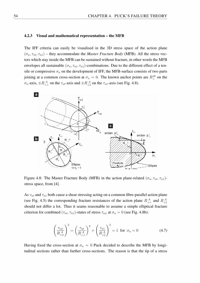
54 CHAPTER 4. PUCK’S FAILURE THEORY
4.2.3 Visual and mathematical representation – the MFB
The IFF criteria can easily be visualised in the 3D stress space of the action plane(𝜎𝑛, 𝜏𝑛𝑡, 𝜏𝑛1) – they accommodate the Master Fracture Body (MFB). All the stress vec-tors which stay inside the MFB can be sustained without fracture, in other words the MFBenvelopes all sustainable (𝜎𝑛, 𝜏𝑛𝑡, 𝜏𝑛1)-combinations. Due to the different effect of a ten-sile or compressive 𝜎𝑛 on the development of IFF, the MFB-surface consists of two partsjoining at a common cross-section at 𝜎𝑛 = 0. The known anchor points are 𝑅𝐴𝑡
⊥ on the𝜎𝑛-axis, ±𝑅 𝐴
⊥⊥ on the 𝜏𝑛𝑡-axis and ±𝑅 𝐴⊥∥ on the 𝜏𝑛1-axis (see Fig. 4.8).
a
b
c
3
A
A
A
t
At
At
Figure 4.8: The Master Fracture Body (MFB) in the action plane-related (𝜎𝑛, 𝜏𝑛𝑡, 𝜏𝑛1)-stress space, from [4].
As 𝜏𝑛𝑡 and 𝜏𝑛1 both cause a shear stressing acting on a common fibre-parallel action plane(see Fig. 4.5) the corresponding fracture resistances of the action plane 𝑅 𝐴
⊥⊥ and 𝑅 𝐴⊥∥
should not differ a lot. Thus it seams reasonable to assume a simple elliptical fracturecriterion for combined (𝜏𝑛𝑡, 𝜏𝑛1)-states of stress 𝜏𝑛𝜓 at 𝜎𝑛 = 0 (see Fig. 4.8b):
(𝜏𝑛𝜓𝑅 𝐴
⊥𝜓
)2
=
(𝜏𝑛𝑡𝑅 𝐴
⊥⊥
)2
+
(𝜏𝑛1𝑅 𝐴
⊥∥
)2
= 1 for 𝜎𝑛 = 0 (4.7)
Having fixed the cross-section at 𝜎𝑛 = 0 Puck decided to describe the MFB by longi-tudinal sections rather than further cross-sections. The reason is that the tip of a stress
4.2. PUCK’S INTER-FIBRE FRACTURE CRITERION 55
vector, which is proportionally stretched by the stretch factor 𝑓𝑆 (see Sec. 4.2.2), is mov-ing in a longitudinal section of the MFB. This fact leads to a rather simple equation for alongitudinal section.
Those parts of the MFB surface where an applied plane (𝜎2, 𝜏21)-stress combination leadsto a fracture in its own action plane (𝜃𝑓𝑝 = 0∘), can easily be investigated experimentally.This is the case in the whole positive range of 𝜎2 > 0 and a small part of the negative𝜎2 ≈ [−0.4 𝑅𝑐
⊥ ; 0]. Within these two ranges there is 𝜃𝑓𝑝 = 0∘ and accordingly 𝜎2 = 𝜎𝑛,𝜏21 = 𝜏𝑛1 and 𝜏𝑛𝑡 = 0. That means that all the resulting IFF fractures are placed on alongitudinal contour line of the MFB in the (𝜏𝑛𝑡 = 0)-plane.
For positive 𝜎𝑛 the (𝜎𝑛, 𝜏𝑛1)-fracture curve can be described well by a branch of an ellipsewhich cuts the 𝜎𝑛-axis perpendicularly at 𝜎𝑛 = 𝑅𝐴𝑡
⊥ and the positive 𝜏𝑛1-axis at 𝜏𝑛1 = 𝑅 𝐴⊥∥
with a declining slope of about 𝛿𝜏𝑛1
𝛿𝜎𝑛= −0.3 (see Fig. 4.8a). According to Coulomb [84]
the fracture curve continues in the negative 𝜎𝑛-region as an inclined straight line. To en-sure conservative results however, a diminishing dependence of the fracture resistances ofthe action plane against shear from negative 𝜎𝑛 is assumed. Thus Puck chose a paraboliccontour line in this region [4] see p. 54ff. This assumption follows Mohr’s idea that thestrengthening effect of compressive 𝜎𝑛 decreases with growing compressive 𝜎𝑛.
Finally the whole MFB arises from the set of ellipse/parabola-contour lines for all angles𝜓. For positive 𝜎𝑛 the result is a calotte with the utmost point on the 𝜎𝑛-axis at 𝜎𝑛 = 𝑅𝐴𝑡
⊥and 𝜏𝑛𝜓 = 0. Looking in negative 𝜎𝑛-direction, the MFB looks like an infinite, slightlywidening funnel. This meets the fact that 𝜎𝑛 alone never causes fracture. There is alwaysa specific amount of 𝜏𝑛𝜓 necessary for fracture and this amount grows with increasingcompressive 𝜎𝑛.
In the following a contour line of the MFB is described by an ellipse in the 𝜎𝑛 ≥ 0 halfspace and by a parabola in the 𝜎𝑛 < 0 half space:
(𝜏𝑛𝜓𝑅 𝐴
⊥𝜓
)2
+ 𝑐1𝜎𝑛𝑅𝐴𝑡
⊥+ 𝑐2
(𝜎𝑛𝑅𝐴𝑡
⊥
)2
= 1 for 𝜎𝑛 ≥ 0 (4.8)
(𝜏𝑛𝜓𝑅 𝐴
⊥𝜓
)2
+ 𝑐 𝜎𝑛 = 1 for 𝜎𝑛 < 0 (4.9)
The ellipse has to include three anchor points (see Fig. 4.8c) which are[𝜎𝑛
𝜏𝑛𝜓
]=
[𝑅𝐴𝑡
⊥0
]on the 𝜎𝑛-axis and
[0
±𝑅𝐴⊥𝜓
]on the 𝜏𝑛𝜓-axis. (4.10)
56 CHAPTER 4. PUCK’S FAILURE THEORY
With equation 4.1 and the geometric relations 𝜏𝑛𝑡 = 𝜏𝑛𝜓 cos𝜓 and 𝜏𝑛1 = 𝜏𝑛𝜓 sin𝜓 itfollows from equation 4.7:
𝑅 𝐴⊥𝜓 =
⎡⎣(cos𝜓
𝑅 𝐴⊥⊥
)2
+
(𝑠𝑖𝑛𝜓
𝑅 𝐴⊥∥
)2⎤⎦− 1
2
(4.11)
While the ellipse crosses the 𝜎𝑛-axis perpendicularly it should cross the 𝜏𝑛𝜓-axis withan inclination which can be chosen within specific limits (see Eq. 4.12). Recommendedvalues will be presented later in this section.
(𝛿𝜏𝑛𝜓𝛿𝜎𝑛
)𝑒𝑙𝑙𝑖𝑝𝑠𝑒𝜎𝑛=0
=
⎧⎨⎩−𝑝𝑡⊥𝜓 for 𝜏𝑛𝜓 > 0
𝑝𝑡⊥𝜓 for 𝜏𝑛𝜓 < 0(4.12)
The parabola describing the contour line of the MFB in areas 𝜎𝑛 < 0 starts at the anchorpoints
(𝜎𝑛 = 0, 𝜏𝑛𝜓 = ±𝑅 𝐴
⊥𝜓)
and its inclination may differ slightly from the inclinationof the ellipse joining at that point:
(𝛿𝜏𝑛𝜓𝛿𝜎𝑛
)𝑝𝑎𝑟𝑎𝑏𝑜𝑙𝑎𝜎𝑛=0
=
⎧⎨⎩−𝑝𝑐⊥𝜓 for 𝜏𝑛𝜓 > 0
𝑝𝑐⊥𝜓 for 𝜏𝑛𝜓 < 0(4.13)
With the above conditions the constants 𝑐1, 𝑐2 and 𝑐 (see Eqs. 4.8 and 4.9) become
𝑐1 = 2𝑝𝑡⊥𝜓 𝑅
𝐴𝑡⊥
𝑅𝐴⊥𝜓
(4.14)
𝑐2 = 1− 2𝑝𝑡⊥𝜓 𝑅
𝐴𝑡⊥
𝑅 𝐴⊥𝜓
(4.15)
𝑐 = 2𝑝𝑐⊥𝜓𝑅𝐴
⊥𝜓. (4.16)
For the inclination values at 𝜓 = 90∘, that means the longitudinal section of the MFBwhere only 𝜎𝑛 and 𝜏𝑛1 exist (𝜏𝑛𝑡 = 0), there is some experimental experience concerningthe inclination parameters 𝑝𝑡⊥𝜓 and 𝑝𝑐⊥𝜓 which are named 𝑝𝑡⊥∥ and 𝑝𝑐⊥∥ in that particularcase. The present analysis follows the recommendations given in [88, 89] also for thevalues 𝑝𝑡⊥⊥ and 𝑝𝑐⊥⊥ valid in the longitudinal section of the MFB at 𝜓 = 0∘ (see Tab. 4.1).
Having chosen the inclinations of the contour lines at 𝜓 = 0∘ and 90∘, Puck uses thefollowing interpolation procedure (see Eq. 4.17) to define the values of 𝑝𝑡⊥𝜓 and 𝑝𝑐⊥𝜓 at
4.2. PUCK’S INTER-FIBRE FRACTURE CRITERION 57
𝑝𝑡⊥∥ 𝑝𝑐⊥∥ 𝑝𝑡⊥⊥, 𝑝𝑐⊥⊥GFRP 0.30 0.25 0.20 to 0.25CFRP 0.35 0.30 0.25 to 0.30
Table 4.1: Recommended inclination parameters.
any angle 𝜓. The procedure ensures a harmonic behaviour of the change in inclinationaround the circumference of the MFB.
𝑝𝑡,𝑐⊥𝜓𝑅𝐴
⊥𝜓=𝑝𝑡,𝑐⊥⊥𝑅𝐴
⊥⊥cos2 𝜓 +
𝑝𝑡,𝑐⊥∥𝑅𝐴
⊥∥sin2 𝜓 (4.17)
with
cos2 𝜓 =𝜏 2𝑛𝑡
𝜏 2𝑛𝑡 + 𝜏 2𝑛1(4.18)
and
sin2 𝜓 =𝜏 2𝑛1
𝜏 2𝑛𝑡 + 𝜏 2𝑛1(4.19)
With equation 4.7 the MFB is completely described by equations 4.8 and 4.9 which arepolynomials of second order of the stresses. The right hand side of the equations setto one makes them a fracture condition. This means, 𝜎𝑛 and 𝜏𝑛𝜓 calculated using theseequations are stresses at IFF. If stresses lower than these are inserted in the left hand sideof the equations 4.8 and 4.9, the result is a figure lower than one. Though this indicates,that these stresses are bearable without IFF, the figure itself does not represent the stressexposure (see Sec. 4.2.2). It was stated that the stress exposure 𝑓𝐸 should increase linearlywith proportionally increasing stresses – this is not the case in the quadratic equations 4.8and 4.9. Thus they have to be rearranged to form a homogeneous function in the firstdegree of the stresses. This can be easily achieved by dividing the stress terms of thefirst order by 𝑓𝐸 and those of the second order by 𝑓 2
𝐸 . Then the general solution of theresulting quadratic equation for 𝑓𝐸 can be written
𝑓𝐸 =1
2
(∑𝐿+
√(∑𝐿)2
+ 4∑
𝑄
)(4.20)
where∑𝐿 is the sum of the stress terms of first order,
∑𝑄 the sum of those of second
order. Applying this term to the fracture conditions (Eqs. 4.8 and 4.9) leads to the twocentral expressions of Puck’s IFF criterion:
58 CHAPTER 4. PUCK’S FAILURE THEORY
𝑓𝐸 𝐼𝐹𝐹 (𝜃) =
√√√√√⎷[(
1
𝑅𝐴𝑡⊥
− 𝑝𝑡⊥𝜓𝑅𝐴
⊥𝜓︸︷︷︸Eq. 4.23
)𝜎𝑛(𝜃)
]2+
(𝜏𝑛𝑡(𝜃)
𝑅𝐴⊥⊥︸︷︷︸
Eq. 4.6
)2
+
(𝜏𝑛1(𝜃)
𝑅𝐴⊥∥
)2
+𝑝𝑡⊥𝜓𝑅𝐴
⊥𝜓︸︷︷︸Eq. 4.23
𝜎𝑛(𝜃)
(4.21)
for 𝜎𝑛 ≥ 0 and
𝑓𝐸 𝐼𝐹𝐹 (𝜃) =
√√√√√⎷(𝜏𝑛𝑡(𝜃)
𝑅𝐴⊥⊥︸︷︷︸
Eq. 4.6
)2
+
(𝜏𝑛1(𝜃)
𝑅𝐴⊥∥
)2
+
(𝑝𝑐⊥𝜓𝑅𝐴
⊥𝜓︸︷︷︸Eq. 4.23
𝜎𝑛(𝜃)
)2
+𝑝𝑐⊥𝜓𝑅𝐴
⊥𝜓︸︷︷︸Eq. 4.23
𝜎𝑛(𝜃) (4.22)
for 𝜎𝑛 < 0
where
𝑝𝑡,𝑐⊥𝜓𝑅𝐴
⊥𝜓=
𝑝𝑡,𝑐⊥⊥𝑅𝐴
⊥⊥︸︷︷︸Eq. 4.6
cos2 𝜓︸ ︷︷ ︸Eq. 4.18
+𝑝𝑡,𝑐⊥∥𝑅𝐴
⊥∥sin2 𝜓︸ ︷︷ ︸Eq. 4.19
(4.23)
Setting 𝑓𝐸 = 1 and 𝜃 = 𝜃𝑓𝑝, equations 4.21 and 4.22 are a different form of the fracturecondition equations 4.8 and 4.9.
Using these two equations (Eqs. 4.21 and 4.22) the orientation 𝜃𝑓𝑝 of the expected fractureplane can be identified:
[𝑓𝐸 𝐼𝐹𝐹 (𝜃)]𝑚𝑎𝑥 = 𝑓𝐸 𝐼𝐹𝐹 (𝜃𝑓𝑝) (4.24)
The associated value of the stress exposure is generally referred to as 𝑓𝐸 𝐼𝐹𝐹 associatedwith a specific state of applied stress and is also the central parameter for the post-failuredegradation analysis (see Ch. 5).
4.2.4 IFF fracture modes classification for 3D analysis
In the design of critical components it is of extraordinary importance to know, whichstresses and strengths of the material are of primary relevance for a failure. RegardingIFF, Puck’s action plane-related fracture criteria now offer the relevant information byidentifying the orientation of the fracture plane and the stresses acting on it.
4.2. PUCK’S INTER-FIBRE FRACTURE CRITERION 59
In his first publication about the new fracture plane-related IFF criteria [21] Puck hasextensively discussed the general shape of the experimentally well captured (𝜎2, 𝜏21)-fracture curve (see Fig. 4.6) and the basic observations associated with the occurringfracture plane orientations. These observations led to the distinction of three differentsections of the fracture curve. Starting from 𝜎2 = 𝑅𝑡
⊥, via 𝜏21 = 𝑅⊥∥ and ending at𝜎2 = −𝑅𝑐
⊥ (see Fig. 4.6) there consecutively occur different stress combinations on thefracture plane leading to different modes of IFF (see Tab. 4.2).
The most important conclusion from the considerations above is: All the presented frac-ture modes are described exclusively by equations 4.21 and 4.22. This is possible due toa two-stage analysis: First the criteria are used to identify the orientation of the fractureplane 𝜃𝑓𝑝 and in a second step they are used to calculate the fracture stresses on that veryplane.
The application of an arbitrary 3D load could potentially produce more states of stress onthe fracture plane than those encountered under 2D load. The most likely case is that allthe three stresses 𝜎𝑛, 𝜏𝑛𝑡 and 𝜏𝑛1 are acting together on the fracture plane. The substantialdifference between all the possible combinations is the algebraic sign of 𝜎𝑛. The mechan-ical difference lies in the fact that a tensile stress 𝜎𝑛 > 0 promotes IFF while compressivestress 𝜎𝑛 < 0 impedes it (see Sec. 4.2.1). Mathematically this fact is expressed by twodifferent fracture conditions, one for positive and one for negative 𝜎𝑛 (see Sec. 4.2.3). It isalso conceivable, that pure shear (𝜏𝑛1 and/or 𝜏𝑛𝑡) acts on the fracture plane. According tothis there is a complete scheme of conceivable stress combinations on the fracture plane(see Tab. 4.3).
Although in the 3D case the categorisation into Modes A, B and C seems no longer ad-equate, the differentiation between fractures with positive or negative 𝜎𝑛 on their frac-ture plane is still significant regarding the consequences of the fracture: While fractureswith 𝜎𝑡𝑛 acting on their fracture plane are generally supposed to be tolerable if the loadcan be redistributed to neighbouring laminae, fracture planes with 𝜎𝑐𝑛 indicate the risk ofan abrupt fatal disintegration (local splitting and delamination) of the laminate by theirwedge effect [6, 39] if a compressive 𝜎2 is present. The considerations above are relevant
Mode A Mode B Mode C𝜃𝑓𝑝 = 0∘ 𝜃𝑓𝑝 = 0∘ 𝜃𝑓𝑝 ∕= 0∘
{𝜎𝑡𝑛 0 0} {𝜎𝑐𝑛 0 𝜏𝑛1} {𝜎𝑐𝑛 𝜏𝑛𝑡 𝜏𝑛1}{𝜎𝑡𝑛 0 𝜏𝑛1} {𝜎𝑐𝑛 𝜏𝑛𝑡 0}{0 0 𝜏𝑛1}
Table 4.2: Possible 2D stress combinations leading to the different IFF fracture modes.
60 CHAPTER 4. PUCK’S FAILURE THEORY
𝜎𝑛 < 0 𝜎𝑛 = 0 𝜎𝑛 > 0
{𝜎𝑐𝑛 𝜏𝑛𝑡 𝜏𝑛1} {0 𝜏𝑛𝑡 𝜏𝑛1} {𝜎𝑡𝑛 𝜏𝑛𝑡 𝜏𝑛1}{𝜎𝑐𝑛 𝜏𝑛𝑡 0} {0 𝜏𝑛𝑡 0} ** {𝜎𝑡𝑛 𝜏𝑛𝑡 0} **{𝜎𝑐𝑛 0 𝜏𝑛1} {0 0 𝜏𝑛1} {𝜎𝑡𝑛 0 𝜏𝑛1}{𝜎𝑐𝑛 0 0} * {𝜎𝑡𝑛 0 0}* A fracture plane on which 𝜎𝑐𝑛 acts exclusively is not conceivablebecause the fracture resistance of the action plane against compres-sive stress is 𝑅𝐴 𝑐
⊥ = ∞ (see Sec. 4.2.3).
** In UD-composites with common ratios between materialstrengths 𝑅𝑐
⊥ and 𝑅𝑡⊥ these combinations do not appear.
Table 4.3: Possible 3D stress combinations on a fracture plane.
for the post-failure degradation analysis and are resumed in chapter 5.
4.3 Influences on the IFF beyond Mohr’s hypothesis
In the context of this section it is important to stress that Puck’s IFF criteria predict brittlemacroscopic IFF failure by means of cracks through the entire thickness of the lamina.Pre-fracture micro-damage-induced constitutive nonlinearities (see Fig. 2.5) are not con-sidered by Puck’s failure theory itself but by the preceding nonlinear stress analysis (seeSec. 3.1.2). However the extended theory accounts for the influence of micro-damage onthe load bearing capacity of the material.
It was previously stated that only stresses acting on the fracture plane (𝜎𝑛, 𝜏𝑛1, 𝜏𝑛𝑡) arerelevant for the fracture itself (see Sec. 4.2). In accordance with Mohr [85], neither thefibre-parallel stress 𝜎1 nor the levels of IFF stress exposures on planes other than thefracture plane have been included so far. Considering the gradual development of anIFF due to the progressive formation of micro cracks and for probabilistic reasons (seeSec. 2.1), there are states of stress where a pure Mohr approach is expected to be on thenon-conservative side. Therefore the following two extensions of the IFF criteria havebeen developed by Puck beyond Mohr’s hypothesis (see Secs. 4.3.1 and 4.3.2).
4.3.1 Influences of fibre-parallel stress 𝜎1
According to Mohr, the stress 𝜎1 does not have any influence on an IFF because that stress’action plane is perpendicular to any possible IFF fracture plane – thus 𝜎𝑛(𝜃), 𝜏𝑛1(𝜃) and𝜏𝑛𝑡(𝜃) are independent from 𝜎1. Experiments, however, have revealed a series of effects
4.3. INFLUENCES ON THE IFF BEYOND MOHR’S HYPOTHESIS 61
which require the inclusion of a 𝜎1-term to reduce the IFF strength somewhat [39]. Themost essential effect is explained by the statistical scatter in the fibre strength. Macro-scopically detected fibre fracture (FF) at ∣𝜎1∣ = 𝑅∥ is the moment, when a very largenumber of elementary fibres breaks and the UD lamina looses most of its load-bearingcapacity in fibre direction. Statistical laws state that some elementary fibres will alreadyhave been broken before the fibre fracture limit 𝑅∥ of the UD lamina has been reached– this is the case for both fibre fractures (tensile 𝜎1) and fibre kinking (compressive 𝜎1).The result of those micro fibre fractures is a local damage of the UD lamina in the formof a local fibre-matrix debonding and micro-fractures in the highly loaded neighbouringmatrix material [10]. They weaken the overall fibre-matrix cohesion and thus reduce itsresistance against IFF.
In order to include the weakening effect of 𝜎1 in the IFF analysis, the fracture resistancesof the action planes are reduced by a weakening factor 𝜂𝑤1 = [0; 1]. This factor canbe used in the tensile and compressive range of 𝜎1 in the same way. For the sake ofsimplicity 𝜂𝑤1 has the same value for all the three fracture resistances 𝑅𝐴𝑡
⊥ , 𝑅𝐴⊥⊥ and 𝑅𝐴
⊥∥.This assumption has the effect that the orientation of the fracture plane 𝜃𝑓𝑝 is independentfrom 𝜂𝑤1 since 𝜎1 is independent from 𝜃 [4]. That means the identification of the fractureplane will be carried out the same way whether including the 𝜎1-influence or not.
ii
i
iii
hw1
fE FF
fE IFF
s1
s2
1
1
-
Figure 4.9: (𝜎1, 𝜎2)-fracture curve including the 𝜎1-influence on IFF.
Regarding the definition of 𝜂𝑤1, the considerations of Puck and Schurmann [6, 39] maybe explained by studying the fracture curve of a simple (𝜎2, 𝜎1)-load case (see Fig. 4.9)in the first quadrant. Gradually starting at a specific 𝜎1-value (horizontal tangent, seeFig. 4.9, i) the weakening effect increases with increasing 𝜎1 but presumably leaves someIFF fracture resistance when reaching the fibre fracture limit (ii). Hence the weakening isdescribed by a fracture curve in the form of a segment of an ellipse. The segment startsat 𝑠 ⋅ 𝑅∥(𝑠 = [0; 1]) and ends at the FF-limit ∣𝜎1∣ = 𝑅∥. Here, the bearable 𝜎2 reaches its
62 CHAPTER 4. PUCK’S FAILURE THEORY
minimum 𝑚 ⋅ 𝑅𝑡⊥(𝑚 = [0; 1]). Both 𝑚 and 𝑠 can be chosen freely between their limits
and may differ for compressive or tensile 𝜎1. Without adequate experimental results thecurrently suggested values are 𝑚 = 𝑠 = 0.5 [88] but as soon as the authors get to knowrelevant data these parameters may be adjusted.
Aiming on the stress exposures 𝑓𝐸 𝐹𝐹 and 𝑓𝐸 𝐼𝐹𝐹 being the central parameters in the 𝜂𝑤1-definition also, the (𝜎2, 𝜎1)-fracture curve may be transferred into a 𝑓𝐸 𝐼𝐹𝐹 (𝜎2) against𝑓𝐸 𝐹𝐹 (𝜎1) curve by dividing 𝜎2 by 𝑅𝑡
⊥ or −𝑅𝑐⊥ and 𝜎1 by 𝑅𝑡
∥ or −𝑅𝑐∥, respectively. This
operation results in solely positive values between [0; 1] and now the former curves ofquadrant 1 and 4 coincide in one curve valid for tensile 𝜎1 and the former curves ofquadrant 2 and 3 coincide in another curve valid for compressive 𝜎1 – now both in thefirst quadrant. If compressive and tensile 𝜎1 are treated equally regarding 𝑠 and 𝑚, bothremaining curves are identical and for simplicity reasons this case is shown in figure 4.9.
Accepting the hypothesis above, that high 𝜎1 – hence high fibre fracture stress exposure𝑓𝐸 𝐹𝐹 (see Sec. 4.7) – weakens all the IFF fracture resistances of all the action planes inthe same way, the considerations may be continued without distinction whether 𝜎2 or anyother combination of applied stresses leads to the IFF. Thus the first quadrant of figure 4.9simultaneously shows the generally bearable 𝑓𝐸 𝐼𝐹𝐹 against 𝑓𝐸 𝐹𝐹 . In order to stick to thegeneral fracture condition 𝑓𝐸 = 1, the bearable IFF stress exposure 𝑓𝐸 𝐼𝐹𝐹 is correctedby (𝜂𝑤1)
−1 which represents a reduction of the fracture resistances:
𝑓𝐸 𝐼𝐹𝐹𝑤1 =𝑓𝐸 𝐼𝐹𝐹 (𝜃𝑓𝑝)
𝜂𝑤1(4.25)
Setting 𝑓𝐸 𝐼𝐹𝐹 = 1 (fracture condition) in equations 4.21 and 4.22 and multiplying all thefracture resistances of the action planes by the same 𝜂𝑤1-value, it may be brought to theleft hand side and accordingly the first quadrant of figure 4.9 also shows the value of 𝜂𝑤1against 𝑓𝐸 𝐹𝐹 . The weakening factor 𝜂𝑤1 (𝑓𝐸 𝐹𝐹 ) is now defined by an elliptical functionfor 𝑓𝐸 𝐹𝐹 = [𝑠; 1]:
𝜂𝑤1 (𝑓𝐸 𝐹𝐹 ) =
√1− (𝑓𝐸 𝐹𝐹 − 𝑠)2
𝑎2with 𝑎 =
1− 𝑠√1−𝑚2
(4.26)
Now that we have defined the conditions on the fracture curve we address a general loadcase:An 𝜂𝑤1-value is not only valid for a specific point on the fracture curve but it is applied toall the load cases whose proportional increase leads to that specific fracture (see Eq. 4.25).The set of these load cases forms a straight line in figure 4.9, iii with an equal ratiobetween 𝑓𝐸 𝐼𝐹𝐹 and 𝑓𝐸 𝐹𝐹 . Accordingly the correlation 𝜂𝑤1 (𝑓𝐸 𝐹𝐹 ) has to be transferred
4.3. INFLUENCES ON THE IFF BEYOND MOHR’S HYPOTHESIS 63
into 𝜂𝑤1(𝑓𝐸 𝐼𝐹𝐹
𝑓𝐸 𝐹𝐹
). The relation between 𝑓𝐸 𝐼𝐹𝐹
𝑓𝐸 𝐹𝐹and 𝑓𝐸 𝐹𝐹 is given by the fact that 𝑓𝐸 𝐹𝐹
is the abscissa value of the intersection between the line and the segment of the ellipse:
𝑓𝐸 𝐹𝐹 =𝑠+
√𝑠2 − (1 + 𝑎2𝑐2)(𝑠2 − 𝑎2)
1 + 𝑎2𝑐2with 𝑐 =
𝑓𝐸 𝐼𝐹𝐹 (𝜃𝑓𝑝)
𝑓𝐸 𝐹𝐹
(4.27)
Equation 4.27 inserted into equation 4.26 the weakening factor is
𝜂𝑤1
(𝑓𝐸 𝐼𝐹𝐹
𝑓𝐸 𝐹𝐹
)=𝑐(𝑎√𝑐2 (𝑎2 − 𝑠2) + 1 + 𝑠
)(𝑐𝑎)2 + 1
for1
𝑠≥ 𝑓𝐸 𝐼𝐹𝐹 (𝜃𝑓𝑝)
𝑓𝐸 𝐹𝐹
≥ 𝑚 . (4.28)
Note that for 𝑓𝐸 𝐼𝐹𝐹 (𝜃𝑓𝑝)
𝑓𝐸 𝐹𝐹> 1
𝑠, there is no 𝜎1-influence (𝜂𝑤1=1) while for 𝑓𝐸 𝐼𝐹𝐹 (𝜃𝑓𝑝)
𝑓𝐸 𝐹𝐹< 𝑚
there is no IFF [4]see p. 86.
4.3.2 Influence of non-fracture plane stresses
Micromechanical studies show that an IFF does not happen suddenly without any advancenotice (see Sec. 2.3.1). Once the standardised IFF stress exposure
𝑓 ′𝐸 𝐼𝐹𝐹 (𝜃) =
𝑓𝐸 𝐼𝐹𝐹 (𝜃)
𝑓𝐸 𝐼𝐹𝐹 (𝜃𝑓𝑝)(4.29)
exceeds a threshold value of about 𝑓 ′𝐸 𝐼𝐹𝐹 (𝜃) ≈ 0.5, instances of micro-damage to the
fibre-matrix composite will occur which increase progressively with increasing stress ex-posure. In the example of a transverse/longitudinal shear stressing 𝜏⊥∥, these are thefamiliar 45∘ micro cracks (hackles) [21] which are stopped at the fibres and cause tinydebondings. It is only when micro-fractures have exceeded a certain magnitude that theIFF will suddenly occur. Generally the micro-fractures resulting from one or more spe-cific stressings have a weakening effect on the fracture resistances 𝑅𝐴 of all fibre-parallelsections.
Additionally every real fibre-matrix composite contains flaws – in the form of curingcracks, flat air entrapments (voids) or local imperfections in the fibre-matrix bonding.Flaws of that kind do have a sense of direction. There is a high probability that a sectionwith an orientation other than the theoretically defined 𝜃𝑓𝑝 contains a flaw which triggersthe fracture despite its somewhat lower 𝑓𝐸 𝐼𝐹𝐹 (𝜃). This is a probabilistic effect. It addsuncertainty to the prediction of the fracture angle and causes the fracture stresses at IFFto be lower than those calculated following Mohr strictly.
In both examples there is a mixture of effects of micro-damage and of probabilisticeffects – they cannot be treated separately. In the analysis both effects are treated by a
64 CHAPTER 4. PUCK’S FAILURE THEORY
weakening factor 𝜂𝑚+𝑝. Generalising, these examples lead to the following conclusion:
It is to be expected that the effects of micro-damage and probabilistic reducing themagnitude of IFF stresses will rise with the number of fibre-parallel sections whichexperience relatively high IFF stress exposures.
In the following the weakening effect of micro-damage and probabilistics on the loadbearing capacity of the material is discussed by means of combined (𝜎2, 𝜎3)-load caseswith varying ratios. Figure 4.10a presents sections of the fracture curves – the dashedline is the fracture curve predicted by the IFF fracture criterion described above (seeSec. 4.2) whereas the bold line represents the fracture curve including micro-damage andprobabilistic effects as experimentally observed. Figures 4.10b - d show the standardisedstress exposure curves for the three load ratios discussed in detail:
b Solely applied 𝜎2 (𝜎3 = 0) or cases with a small additional amount of 𝜎3 lead toonly few highly stressed action planes in a small interval around the fracture angle𝜃𝑝𝑓 = 0∘. Only few of the contained flaws are sensitive against the applied load anddevelop into correspondingly oriented micro-cracks (see insert). These few micro-defects have only a limited weakening effect on the load bearing capacity of thematerial (see Fig. 4.10a, i). The associated weakening factor 𝜂𝑚+𝑝 is only slightlybelow 1.
c Load cases with a higher ratio between 𝜎3 and 𝜎2 lead to considerably more actionplanes where the threshold for micro-damage (here 𝑓 ′
𝐸 𝐼𝐹𝐹𝑡ℎ𝑟= 0.5 [88]) has been
exceeded. More flaws are activated and develop to micro-defects with a largervariety of orientations (see insert) but their weakening effect is considered to beorientation-independent. The associated weakening factor 𝜂𝑚+𝑝 is noticeably below1 and the fracture curve is accordingly corrected to lower bearable stresses (seeFig. 4.10a, ii).
d Load cases with a 𝜎3/𝜎2-ratio approaching 1 are close to the extreme case whereall the sections are experiencing the same stress exposure, i.e. 𝑓 ′
𝐸 𝐼𝐹𝐹 (𝜃) = 1 =
𝑐𝑜𝑛𝑠𝑡𝑎𝑛𝑡 for 𝜎3 = 𝜎2. Having only tensile load components applied, in case 𝑑the normal stress 𝜎𝑛 is nearly equally high on all action planes and all kinds ofcontained flaws are activated (see insert). The resulting micro-defects significantlyweaken the load bearing capacity of the material which is represented by an associ-ated 𝜂𝑚+𝑝 ≈ 0.7 (see Fig. 4.10a, iii).
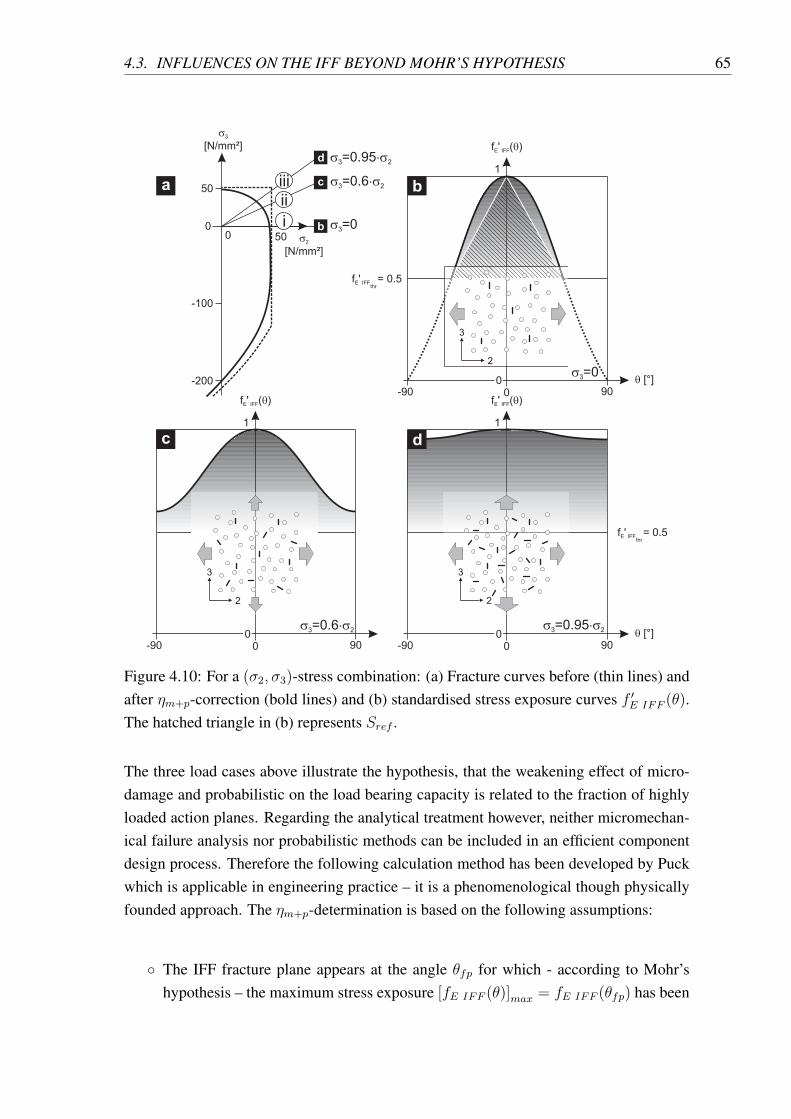
4.3. INFLUENCES ON THE IFF BEYOND MOHR’S HYPOTHESIS 65
c
b
f ' ( )E IFF q
s3
[N/mm²]
s ×s3 2=0.6
s ×s3 2=0.95
50
0 50 s2
[N/mm²]
-100
-200
0 s3=0
= 0.5f 'E IFFthr
-900
0 90q [°]
1
f ' ( )E IFF q
= 0.5f 'E IFFthr
-900
0 90
1
f ' ( )E IFF q
-900
0 90q [°]
1
s ×s3 2=0.6
a
d
2
3
2
3
s ×s3 2=0.95
s3=02
3
ii
i
iii
b
c
d
Figure 4.10: For a (𝜎2, 𝜎3)-stress combination: (a) Fracture curves before (thin lines) andafter 𝜂𝑚+𝑝-correction (bold lines) and (b) standardised stress exposure curves 𝑓 ′
𝐸 𝐼𝐹𝐹 (𝜃).The hatched triangle in (b) represents 𝑆𝑟𝑒𝑓 .
The three load cases above illustrate the hypothesis, that the weakening effect of micro-damage and probabilistic on the load bearing capacity is related to the fraction of highlyloaded action planes. Regarding the analytical treatment however, neither micromechan-ical failure analysis nor probabilistic methods can be included in an efficient componentdesign process. Therefore the following calculation method has been developed by Puckwhich is applicable in engineering practice – it is a phenomenological though physicallyfounded approach. The 𝜂𝑚+𝑝-determination is based on the following assumptions:
∘ The IFF fracture plane appears at the angle 𝜃𝑓𝑝 for which - according to Mohr’shypothesis – the maximum stress exposure [𝑓𝐸 𝐼𝐹𝐹 (𝜃)]𝑚𝑎𝑥 = 𝑓𝐸 𝐼𝐹𝐹 (𝜃𝑓𝑝) has been
66 CHAPTER 4. PUCK’S FAILURE THEORY
calculated (see Eqs. 4.21 and 4.22).
∘ The IFF fracture stresses are obtained by correcting the fracture stresses {𝜎}Mohr𝑓𝑟
calculated from 𝑓𝐸 𝐼𝐹𝐹 (𝜃𝑓𝑝) to lower stresses {𝜎}𝑚+𝑝 using the correction factor𝜂𝑚+𝑝 = [0; 1] (see Eq. 4.30). Correspondingly, the IFF stress exposures calculatedby Mohr 𝑓𝐸 𝐼𝐹𝐹 (𝜃𝑓𝑝) are corrected to higher values 𝑓𝐸 𝐼𝐹𝐹𝑚+𝑝 by dividing them by𝜂𝑚+𝑝 (see Eq. 4.31).
{𝜎}𝑚+𝑝 = {𝜎}Mohr𝑓𝑟 ⋅ 𝜂𝑚+𝑝 =
{𝜎}𝑓𝐸 𝐼𝐹𝐹 (𝜃𝑓𝑝)
⋅ 𝜂𝑚+𝑝 ={𝜎}
𝑓𝐸 𝐼𝐹𝐹𝑚+𝑝
(4.30)
𝑓𝐸 𝐼𝐹𝐹𝑚+𝑝 =𝑓𝐸 𝐼𝐹𝐹 (𝜃𝑓𝑝)
𝜂𝑚+𝑝
or =𝑓𝐸 𝐼𝐹𝐹𝑤1
𝜂𝑚+𝑝
, respectively (4.31)
The integrated amount 𝑆 of standardised stress exposure on all the relevant fibre-parallelsections represents the area below the respective 𝑓 ′
𝐸 𝐼𝐹𝐹 (𝜃)-curve (see Fig. 4.10b) and iscalculated as follows:
𝑆 =
∫all planes*
(𝑓 ′𝐸 𝐼𝐹𝐹 (𝜃)− 𝑓 ′
𝐸 𝐼𝐹𝐹𝑡ℎ𝑟
)𝑑𝜃 ≈
179∘∗∑0∘
(𝑓 ′𝐸 𝐼𝐹𝐹 (𝜃)− 𝑓 ′
𝐸 𝐼𝐹𝐹𝑡ℎ𝑟
) ⋅ △𝜃 (4.32)
* only including planes where 𝑓 ′𝐸 𝐼𝐹𝐹 (𝜃) ≥ 𝑓 ′
𝐸 𝐼𝐹𝐹𝑡ℎ𝑟
The summing formula as presented above is valid for angular increments of △𝜃 = 1∘.The integration or summing with a zero line shifted by 𝑓 ′
𝐸 𝐼𝐹𝐹𝑡ℎ𝑟results in a considerably
higher weight of high 𝑓 ′𝐸 𝐼𝐹𝐹 (𝜃)-values than of low ones.
Puck has described the dependence of 𝜂𝑚+𝑝 on the integrated standardised stress exposure𝑆 by
𝜂𝑚+𝑝 = 1−△𝑚𝑎𝑥𝑆 − 𝑆𝑟𝑒𝑓
𝑆𝑚𝑎𝑥 − 𝑆𝑟𝑒𝑓(4.33)
with 𝑆𝑚𝑎𝑥 = 90∘ and 𝑆𝑟𝑒𝑓 = 30∘ [88].
The reference value 𝑆𝑟𝑒𝑓 achieves a reasonable sensitivity on 𝜂𝑚+𝑝 against the differencesin the 𝑆-values of different states of stress. 𝑆𝑟𝑒𝑓 represents large parts of that area belowthe standardised stress exposure curve which is already contained below a uniaxial loadcase curve (see Fig. 4.10b, hatched triangle) and hence contained below every standard-ised stress exposure. The value △𝑚𝑎𝑥 = [0.15; 0.25] calibrates the 𝜂𝑚+𝑝-correction.
Note that {𝜎}Mohr𝑓𝑟 and 𝑓𝐸 𝐼𝐹𝐹 (𝜃𝑓𝑝) (Eqs. 4.30 and 4.31) have to be calculated by a cor-
rected set of material parameters. The reason is that the experimentally determined
4.3. INFLUENCES ON THE IFF BEYOND MOHR’S HYPOTHESIS 67
strengths 𝑅𝑡⊥, 𝑅𝑐
⊥ and 𝑅⊥∥ (the anchor points of the IFF criteria) ab initio include micro-damage and probabilistic effects. Thus the analytical procedure of the 𝜂𝑚+𝑝-correctionsshould not degrade these values a second time – the experimentally measured basic ma-terial strengths have just to be met by an analysis including 𝜂𝑚+𝑝.
Correcting the material strengths suggests the correction of the inclination parameters 𝑝𝑡,𝑐⊥∥and 𝑝𝑡,𝑐⊥⊥, too. This matter is discussed in detail in [4] see p. 94ff but up to now the exper-imental data is limited to (𝜎2, 𝜏21)-fracture curves which prove the following correctionfor 𝑝𝑐⊥∥:
𝑝𝑐⊥∥ 𝑐𝑜𝑟𝑝𝑐⊥∥
= 1 + 0.6 ⋅ △𝑚𝑎𝑥
𝑝𝑐⊥∥(4.34)
for 0.15 ≤ △𝑚𝑎𝑥 ≤ 0.25 and 0.25 ≤ 𝑝𝑐⊥∥ ≤ 0.35
The remaining inclination parameters 𝑝𝑡⊥∥ and 𝑝𝑡,𝑐⊥⊥ stay unmodified for the time being.
The corrected strengths 𝑅𝑡⊥ 𝑐𝑜𝑟, 𝑅
𝑐⊥ 𝑐𝑜𝑟 and 𝑅⊥∥ 𝑐𝑜𝑟 on which a fracture analysis including
the 𝜂𝑚+𝑝-corrections has to be based are derived by
𝑅𝑐𝑜𝑟 =𝑅
𝜂𝑚+𝑝
(4.35)
The 𝜂𝑚+𝑝-values in the denominator have to be calculated from the respective load cases– uniaxial tension 𝜎𝑡⊥, uniaxial compression 𝜎𝑐⊥ and pure inplane shear 𝜏⊥∥ – by equa-tions 4.32 and 4.33. The fact that the calculation of the 𝑓 ′
𝐸 𝐼𝐹𝐹 (𝜃)-values should alreadybe based on corrected strengths reveals a circular reference. In general this prohibits aclosed-form solution but the problem may easily be solved using contemporary numeri-cal software.
Regarding the pure inplane shear case 𝜏⊥∥, such a procedure can be omitted due to thefact that 𝜏⊥∥(𝜃) = cos(𝜃) ⋅ 𝜏21 is the only stress component on any action plane. Usingthe standardised stress exposure in equation 4.32, the values 𝑅⊥∥ or 𝑅⊥∥ 𝑐𝑜𝑟 are of noimportance and 𝑆⊥∥ = 39, 24∘ exclusively results from the integration of the cosine shapeof 𝑓 ′
𝐸 𝐼𝐹𝐹 (𝜃) independent from the material. The result is the value 𝑅⊥∥ 𝑐𝑜𝑟 which exactlymeets the fracture condition 𝑓𝐸 𝐼𝐹𝐹𝑚+𝑝 = 1 for an applied inplane shear of 𝜏21 = 𝑅⊥∥.
The uniaxial compression case may be simplified accordingly: Using equation 4.6 andassuming an unmodified 𝑝𝑐⊥⊥, the compressive strength 𝑅𝑐
⊥ remains the only material pa-rameter and vanishes after the the standardisation (Eq. 4.29). Hence the value 𝑆𝑐⊥ dependson 𝑝𝑐⊥⊥ only and is about 36∘ for the suggested values of 𝑝𝑐⊥⊥ (see Tab. 4.1). The result-ing 𝑅𝑐
⊥ 𝑐𝑜𝑟 leads to 𝑓𝐸 𝐼𝐹𝐹𝑚+𝑝 = 1 for an applied 𝜎2 = −𝑅𝑐⊥. Equation 4.6 provides the
associated 𝑅𝐴⊥⊥ 𝑐𝑜𝑟.
68 CHAPTER 4. PUCK’S FAILURE THEORY
Only in the case of a uniaxial tension there are more than one mutually independentmaterial parameters relevant in equation 4.21 and the shape of 𝑓 ′
𝐸 𝐼𝐹𝐹 (𝜃) depends onboth, 𝑅𝐴
⊥⊥ 𝑐𝑜𝑟 and 𝑅𝑡⊥ 𝑐𝑜𝑟 (assuming an unmodified 𝑝𝑡⊥⊥). However, using the 𝑅𝐴
⊥⊥ 𝑐𝑜𝑟
defined in the step above, an 𝑅𝑡⊥ 𝑐𝑜𝑟 can be found which leads to 𝑓𝐸 𝐼𝐹𝐹𝑚+𝑝 = 1 for an
applied 𝜎2 = 𝑅𝑡⊥. The 𝜂𝑚+𝑝-influence for this load case is expected to be rather small
and may be neglected if no adequate numerical software is at hand. In general it is highlyadvisable to use the 𝜂𝑚+𝑝-corrections. Even if based on uncorrected material parametersthe IFF prediction including 𝜂𝑚+𝑝 will be more accurate than any analysis neglecting theinfluence of micro-damage and probabilistics.
4.4 Puck’s IFF criteria and the Mohr’ circle
It has been stated that Puck’s Theory for IFF is based on Coulomb’s and Mohr’s fracturecriterion (see Sec. 4.2). In the following section the relation between Puck’s action plane-related IFF criterion and Mohr’s perception of stresses is outlined.
The Mohr’s circle of stresses is a graphical approach to derive the stress components(𝜎𝐴, 𝜏𝐴
)acting on an arbitrary section 𝐴 due to applied plane stress (𝜎𝑥, 𝜎𝑦, 𝜏𝑥𝑦) (see
Fig. 4.11a). Figure 4.11c defines the relevant orientations and includes the principalstresses associated with the applied load. It is these principal stresses, between whichthe Mohr’s circle is spanned (c) but it may also be constructed by the following definitionof its centre and radius:
𝜎𝑀 =1
2(𝜎𝑥 + 𝜎𝑦) (4.36)
𝑟 =
√(𝜎𝑥 − 𝜎𝑦
2
)2
+ 𝜏 2𝑥𝑦 (4.37)
Neglecting the 1-direction, the situation described above is equivalent to a lamina sub-jected to the fibre-perpendicular stress components (𝜎2, 𝜎3, 𝜏23) (b) and thus the Mohr’scircle also provides the possible combinations (𝜎𝑛, 𝜏𝑛𝑡) of all the relevant action planesin a lamina (see Fig. 4.5). Transferred to the lamina the abscissa has the meaning of an𝜎𝑛-axis and the ordinate of an 𝜏𝑛𝑡-axis. Interpreted in that sense, the Mohr’s circle asso-ciated with a particular state of stress in a lamina may be combined with the illustrationof the Master Fracture Body (see Sec. 4.2.3). The Mohr’s circle lies in the 𝜎𝑛-𝜏𝑛𝑡-planeof the MFB and serves as the basis for the additional shear components 𝜏𝑛1 (𝜃) followingequation 4.3. They are plotted as a vertical vector starting from the respective position onthe Mohr’s circle. The result is a closed curve in the (𝜎𝑛, 𝜏𝑛𝑡, 𝜏𝑛1)-space which representsthe set of possible stress combinations acting on all the action planes (see Fig. 4.12). As
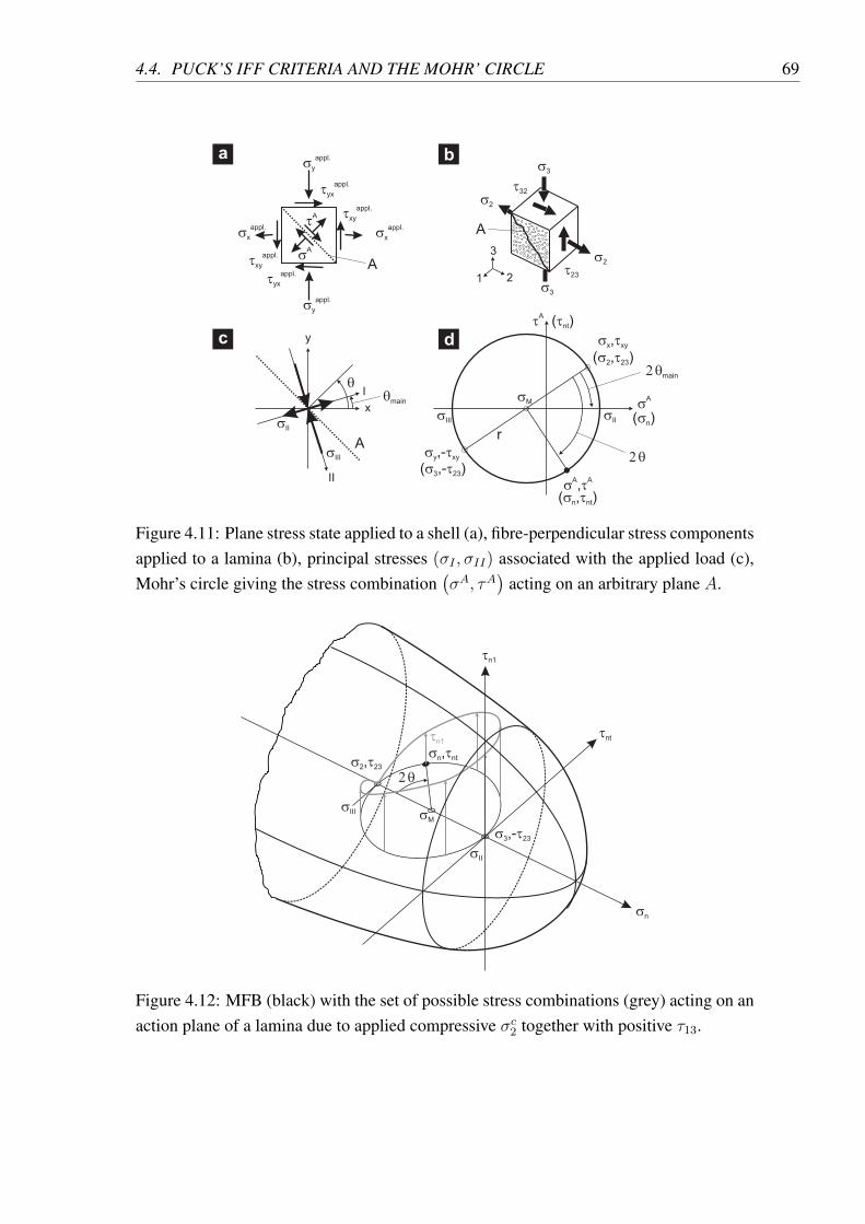
4.4. PUCK’S IFF CRITERIA AND THE MOHR’ CIRCLE 69
1
3
2
a b
txy
appl.
sy
appl.
sy
appl.
sx
appl.sx
appl.
tyx
appl.
tyx
appl.
txy
appl.
s3
s2
t23
t32
s3
s2
sA
tA
sA
tA
sIIsIII
x
y
I
II
sII
sIII
s tx xy,
s ty xy,-
qmain
q2 qmain
2 q
s tA A,
c d
A
A
A
sM
r
( , )s t2 23
( ,- )s t3 23
( , )s tn nt
( )sn
( )tnt
Figure 4.11: Plane stress state applied to a shell (a), fibre-perpendicular stress componentsapplied to a lamina (b), principal stresses (𝜎𝐼 , 𝜎𝐼𝐼) associated with the applied load (c),Mohr’s circle giving the stress combination
(𝜎𝐴, 𝜏𝐴
)acting on an arbitrary plane 𝐴.
sII
sIII
2 q
sM
s t2 23,
s t3 23,-
s tn nt,
sn
tnt
tn1
tn1
Figure 4.12: MFB (black) with the set of possible stress combinations (grey) acting on anaction plane of a lamina due to applied compressive 𝜎𝑐2 together with positive 𝜏13.
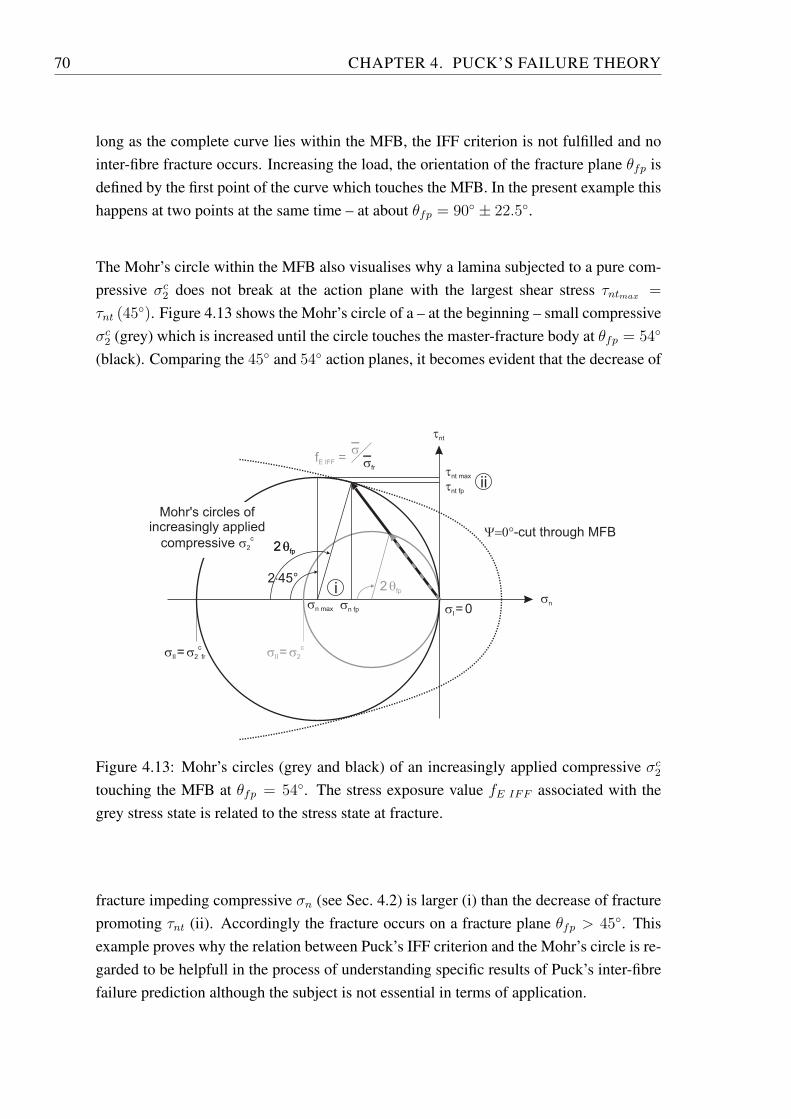
70 CHAPTER 4. PUCK’S FAILURE THEORY
long as the complete curve lies within the MFB, the IFF criterion is not fulfilled and nointer-fibre fracture occurs. Increasing the load, the orientation of the fracture plane 𝜃𝑓𝑝 isdefined by the first point of the curve which touches the MFB. In the present example thishappens at two points at the same time – at about 𝜃𝑓𝑝 = 90∘ ± 22.5∘.
The Mohr’s circle within the MFB also visualises why a lamina subjected to a pure com-pressive 𝜎𝑐2 does not break at the action plane with the largest shear stress 𝜏𝑛𝑡𝑚𝑎𝑥 =
𝜏𝑛𝑡 (45∘). Figure 4.13 shows the Mohr’s circle of a – at the beginning – small compressive
𝜎𝑐2 (grey) which is increased until the circle touches the master-fracture body at 𝜃𝑓𝑝 = 54∘
(black). Comparing the 45∘ and 54∘ action planes, it becomes evident that the decrease of
tnt fp
tnt max
Y=0°-cut through MFB
tnt
sn
sI=0
s sII 2=c
2 qfp
2 45°×2 qfp
2 qfp
sII= s2 fr
c
sn fpsn max
Mohr's circles ofincreasingly applied
compressive s2
c
f =E IFF sfr
s
i
ii
Figure 4.13: Mohr’s circles (grey and black) of an increasingly applied compressive 𝜎𝑐2touching the MFB at 𝜃𝑓𝑝 = 54∘. The stress exposure value 𝑓𝐸 𝐼𝐹𝐹 associated with thegrey stress state is related to the stress state at fracture.
fracture impeding compressive 𝜎𝑛 (see Sec. 4.2) is larger (i) than the decrease of fracturepromoting 𝜏𝑛𝑡 (ii). Accordingly the fracture occurs on a fracture plane 𝜃𝑓𝑝 > 45∘. Thisexample proves why the relation between Puck’s IFF criterion and the Mohr’s circle is re-garded to be helpfull in the process of understanding specific results of Puck’s inter-fibrefailure prediction although the subject is not essential in terms of application.
4.5. CONFINED LAMINAE – THE IN-SITU EFFECT 71
4.5 Confined laminae – the In-Situ Effect
When confined into a laminate, the lamina’s IFF strengths are observed to be higher thanmeasured in isolated UD laminae [90]. The lay-up configuration apparently obstructsthe development of Mode A and B cracks (see Sec. 4.2.4). While the effect itself isindisputable, there is only little information on its quantity. Therefore in all the laminatetest cases (cases 8 to 12) the measured basic strengths are multiplied with the followingroughly estimated factors:
∘ Inplane transverse tensile strength 𝑅𝑡⊥2: 1.35
∘ Inplane transverse/longitudinal shear strength 𝑅⊥∥21: 1.175
The transverse compressive strength 𝑅𝑐⊥2 and the through-thickness strengths including
shear (𝑅𝑡/𝑐⊥3 and 𝑅⊥∥31) are assumed to be unaffected. While the present implementation
accounts for different values for 𝑅𝑡⊥2 and 𝑅𝑡
⊥3 (see Sec. 7.2.2) it enforces 𝑅⊥∥21 = 𝑅⊥∥31.Furthermore, the present implementation does not yet distinguish between embedded andouter plies, although it is known that the in-situ effect on outer plies is smaller if notnegligible. Taking into account the in-situ effect by increasing the strengths of materialsis another case where the given nonlinear stress-strain relations are exceeded as they endat the original strengths. Thus the affected curves have been scaled in a self-similar wayaccording to section 3.1.2.
4.6 Application of Puck’s IFF criterion to special cases
4.6.1 Application to isotropic material
The fundamental difference between fracture of a UD-composite and an isotropic purematrix material is that in the latter case the fracture may occur in a plane at any orientation(𝜃, 𝜑) (see Fig. 4.14). In a UD-composite fracture may only occur in planes parallel to thefibres and thus one angle 𝜃 unambiguously defines possible fracture planes (see Fig. 4.5).
Therefore in the isotropic case, the stresses acting on an action plane are 𝜎𝑛(𝜃, 𝜑) and𝜏𝑛𝜓(𝜃, 𝜑). Once these stresses are calculated from the applied stresses [91], the searchfor the plane with the largest stress exposure may be performed using a slightly modifiedformulation of the usual 𝑓𝐸 now depending on (𝜃, 𝜑):
In an isotropic material there are no different fracture resistances of the action planeagainst the two shear stresses 𝜏𝑛1 and 𝜏𝑛𝑡 and accordingly 𝑅𝐴
⊥⊥ and 𝑅𝐴⊥∥ can be replaced
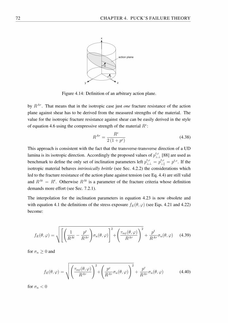
72 CHAPTER 4. PUCK’S FAILURE THEORY
x
zy
action plane
q
j
Figure 4.14: Definition of an arbitrary action plane.
by 𝑅𝐴𝜏 . That means that in the isotropic case just one fracture resistance of the actionplane against shear has to be derived from the measured strengths of the material. Thevalue for the isotropic fracture resistance against shear can be easily derived in the styleof equation 4.6 using the compressive strength of the material 𝑅𝑐:
𝑅𝐴𝜏 =𝑅𝑐
2 (1 + 𝑝𝑐)(4.38)
This approach is consistent with the fact that the transverse-transverse direction of a UDlamina is its isotropic direction. Accordingly the proposed values of 𝑝𝑡,𝑐⊥⊥ [88] are used asbenchmark to define the only set of inclination parameters left 𝑝𝑡,𝑐⊥⊥ = 𝑝𝑡,𝑐⊥∥ = 𝑝𝑡,𝑐. If theisotropic material behaves intrinsically brittle (see Sec. 4.2.2) the considerations whichled to the fracture resistance of the action plane against tension (see Eq. 4.4) are still validand 𝑅𝐴𝑡 = 𝑅𝑡. Otherwise 𝑅𝐴𝑡 is a parameter of the fracture criteria whose definitiondemands more effort (see Sec. 7.2.1).
The interpolation for the inclination parameters in equation 4.23 is now obsolete andwith equation 4.1 the definitions of the stress exposure 𝑓𝐸(𝜃, 𝜑) (see Eqs. 4.21 and 4.22)become:
𝑓𝐸(𝜃, 𝜑) =
√√√⎷[( 1
𝑅𝐴𝑡− 𝑝𝑡
𝑅𝐴𝜏
)𝜎𝑛(𝜃, 𝜑)
]2+
(𝜏𝑛𝜓(𝜃, 𝜑)
𝑅𝐴𝜏
)2
+𝑝𝑡
𝑅𝐴𝜏𝜎𝑛(𝜃, 𝜑) (4.39)
for 𝜎𝑛 ≥ 0 and
𝑓𝐸(𝜃, 𝜑) =
√√√⎷(𝜏𝑛𝜓(𝜃, 𝜑)𝑅𝐴𝜏
)2
+
(𝑝𝑐
𝑅𝐴𝜏𝜎𝑛(𝜃, 𝜑)
)2
+𝑝𝑐
𝑅𝐴𝜏𝜎𝑛(𝜃, 𝜑) (4.40)
for 𝜎𝑛 < 0
4.6. APPLICATION OF PUCK’S IFF CRITERION TO SPECIAL CASES 73
For the sake of simplicity we will assume in the following 𝑝𝑐 = 𝑝𝑡 = 𝑝.
The procedure above leads to a rotationally symmetric MFB (see Fig. 4.8a) with identicallongitudinal sections for any angle 𝜓. This representation equals the reduction of theMFB to a Master Fracture Curve (see Fig. 4.8c) depending only on 𝜎𝑛 and 𝜏𝑛𝜓 as it wasstated for isotropic materials in the very beginning (see Sec. 4.2). It goes without sayingthat in isotropic material neither the 𝑥1-direction does have the usual exceptional positionnor the FF criterion is of any significance.
The modified Puck’s IFF criterion for isotropic material has been applied to the test case1 of the WWFE-II (see Sec. 7.2.1)
4.6.2 Application to not intrinsically brittle materials
While intrinsically brittle behaviour (see Sec. 4.2.2) may be assumed for most FRCs, apure matrix material as given in test case 1 of the WWFE-II (see Sec. 7.2.1) may requirefurther consideration. For MY750 the given shear strength 𝑅𝜏 = 54 MPa is considerablylower than the given tensile strength 𝑅𝑡 = 80 MPa (see App. B.2). Applied shear stressleads to a maximum tensile stress 𝜎𝑡𝑛 of equal magnitude on a section inclined by 45∘. Soif the given material was intrinsically brittle, then 𝑅𝜏 would be close or equal to 𝑅𝑡 andthis section would be the fracture plane. As this is obviously not the case here, fractureis probably driven by a mixed-mode stressing (𝜎𝑛, 𝜏𝑛𝜓) on the fracture plane. Havingdetected this behaviour for an applied pure shear stress, there is no reason to expect ex-clusively 𝜎𝑡𝑛-driven fractures due to an applied uniaxial tensile stress – a mixed-modefracture on a section inclined against the action plane of the applied uniaxial tension willprobably occur. Thus equation 4.4 is no longer valid and there are now two unknowns,mutually dependent model parameters to determine: 𝑝 and 𝑅𝐴𝑡.
As the calibration of the model demands the determination of two parameters, we usethose two given states of stress leading to fracture (𝜎𝑡 = 𝑅𝑡 and 𝜏 = 𝑅𝜏 ) which havenot yet been incorporated into any other relation (𝜎𝑐 = −𝑅𝑐 is already used in equa-tion 4.38). For both cases it is possible to determine the set of value pairs (𝑅𝐴𝑡, 𝑝) wherethe model exactly predicts the given failure stresses for uniaxial tension and pure shear(see Fig. 4.15). The use of an analytical tool is the most efficient way to derive the pre-sented chart [92]. Based on the parameters met by both curves (see Fig. 4.15), the resultsof test case 1 are summarised in figure 7.1.
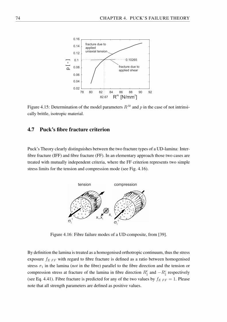
74 CHAPTER 4. PUCK’S FAILURE THEORY
0.02
0.04
0.06
0.08
0.1
0.12
0.14
0.16
78 80 82 84 86 88 90 92
p [
- ]
R [N/mm ]2At
fracture due toapplied shear
fracture due toapplieduniaxial tension
0.10265
82.67
Figure 4.15: Determination of the model parameters 𝑅𝐴𝑡 and 𝑝 in the case of not intrinsi-cally brittle, isotropic material.
4.7 Puck’s fibre fracture criterion
Puck’s Theory clearly distinguishes between the two fracture types of a UD-lamina: Inter-fibre fracture (IFF) and fibre fracture (FF). In an elementary approach those two cases aretreated with mutually independent criteria, where the FF criterion represents two simplestress limits for the tension and compression mode (see Fig. 4.16).
tension compression
x^x ,x1 ||
s||
t
s||
c
Figure 4.16: Fibre failure modes of a UD-composite, from [39].
By definition the lamina is treated as a homogenised orthotropic continuum, thus the stressexposure 𝑓𝐸 𝐹𝐹 with regard to fibre fracture is defined as a ratio between homogenisedstress 𝜎1 in the lamina (not in the fibre) parallel to the fibre direction and the tension orcompression stress at fracture of the lamina in fibre direction 𝑅𝑡
∥ and −𝑅𝑐∥ respectively
(see Eq. 4.41). Fibre fracture is predicted for any of the two values by 𝑓𝐸 𝐹𝐹 = 1. Pleasenote that all strength parameters are defined as positive values.
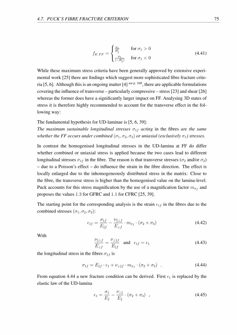
4.7. PUCK’S FIBRE FRACTURE CRITERION 75
𝑓𝐸 𝐹𝐹 =
⎧⎨⎩𝜎1𝑅𝑡
∥for 𝜎1 > 0
𝜎1(−𝑅𝑐
∥)for 𝜎1 < 0
(4.41)
While these maximum stress criteria have been generally approved by extensive experi-mental work [25] there are findings which suggest more sophisticated fibre fracture crite-ria [5, 6]. Although this is an ongoing matter [4] see p. 16ff, there are applicable formulationscovering the influence of transverse – particularly compressive – stress [23] and shear [26]whereas the former does have a significantly larger impact on FF. Analysing 3D states ofstress it is therefore highly recommended to account for the transverse effect in the fol-lowing way:
The fundamental hypothesis for UD-laminae is [5, 6, 39]:The maximum sustainable longitudinal stresses 𝜎1𝑓 acting in the fibres are the samewhether the FF occurs under combined (𝜎1, 𝜎2, 𝜎3) or uniaxial (exclusively 𝜎1) stresses.
In contrast the homogenised longitudinal stresses in the UD-lamina at FF do differwhether combined or uniaxial stress is applied because the two cases lead to differentlongitudinal stresses 𝜎1𝑓 in the fibre. The reason is that transverse stresses (𝜎2 and/or 𝜎3)– due to a Poisson’s effect – do influence the strain in the fibre direction. The effect islocally enlarged due to the inhomogeneously distributed stress in the matrix: Close tothe fibre, the transverse stress is higher than the homogenised value on the lamina-level.Puck accounts for this stress magnification by the use of a magnification factor 𝑚𝜎𝑓 andproposes the values 1.3 for GFRC and 1.1 for CFRC [25, 39].
The starting point for the corresponding analysis is the strain 𝜖1𝑓 in the fibres due to thecombined stresses (𝜎1, 𝜎2, 𝜎3):
𝜖1𝑓 =𝜎1𝑓𝐸∥𝑓
− 𝜈∥⊥𝑓𝐸⊥𝑓
⋅𝑚𝜎𝑓 ⋅ (𝜎2 + 𝜎3) (4.42)
With𝜈∥⊥𝑓𝐸⊥𝑓
=𝜈⊥∥𝑓𝐸∥𝑓
and 𝜖1𝑓 = 𝜖1 (4.43)
the longitudinal stress in the fibres 𝜎1𝑓 is
𝜎1𝑓 = 𝐸∥𝑓 ⋅ 𝜖1 + 𝜈⊥∥𝑓 ⋅𝑚𝜎𝑓 ⋅ (𝜎2 + 𝜎3) . (4.44)
From equation 4.44 a new fracture condition can be derived. First 𝜖1 is replaced by theelastic law of the UD-lamina
𝜖1 =𝜎1𝐸∥
− 𝜈⊥∥𝐸∥
⋅ (𝜎2 + 𝜎3) , (4.45)
76 CHAPTER 4. PUCK’S FAILURE THEORY
then the fibre stress 𝜎1𝑓 by the fracture resistance of the fibre 𝑅∥𝑓
𝑅∥𝑓 = 𝐸∥𝑓 ⋅ 𝜖𝐹𝐹𝑓and 𝑅∥ = 𝐸∥ ⋅ 𝜖𝐹𝐹
with 𝜖𝐹𝐹𝑓=𝜖𝐹𝐹−−−−−−−−→ 𝑅∥𝑓 =
𝐸∥𝑓𝐸∥
⋅𝑅∥ . (4.46)
The resulting FF condition for UD-lamina is:
1
±𝑅𝑡,𝑐∥
[𝜎1 −
(𝜈⊥∥ − 𝜈⊥∥𝑓 ⋅𝑚𝜎𝑓
𝐸∥𝐸∥𝑓
)(𝜎2 + 𝜎3)
]= 1 (4.47)
with
⎧⎨⎩𝑅𝑡∥ for [...] ≥ 0
−𝑅𝑐∥ for [...] < 0
The fracture function is homogeneous of grade 1 and thus can directly be understood as aformulation for the stress exposure 𝑓𝐸 𝐹𝐹 of UD-lamina with regard to fibre fracture:
𝑓𝐸 𝐹𝐹 =1
±𝑅𝑡,𝑐∥
[𝜎1 −
(𝜈⊥∥ − 𝜈⊥∥𝑓 ⋅𝑚𝜎𝑓
𝐸∥𝐸∥𝑓
)(𝜎2 + 𝜎3)
](4.48)
with
⎧⎨⎩𝑅𝑡∥ for [...] ≥ 0
−𝑅𝑐∥ for [...] < 0
Please note that 𝜈⊥∥ and 𝜈⊥∥𝑓 are the major Poisson’s ratios of the UD-lamina and thefibres, respectively. The first index denotes the direction of the lateral strain caused by thestress acting in the direction of the second index.
Puck has found that in the case of plane (𝜎1, 𝜎2, 𝜏21)-stress, the results of equations 4.41and 4.48 differ by only a few percent. However, the influence of transverse stresses onFF can become important in the region of combined compressive 𝜎𝑐2 and 𝜎𝑐3 of similarmagnitude, where ∣𝜎2∣ and ∣𝜎3∣ can exceed the transverse compressive strength 𝑅𝑐
⊥ by afactor of up to 4 [23] (see Sec. 7.2.2).
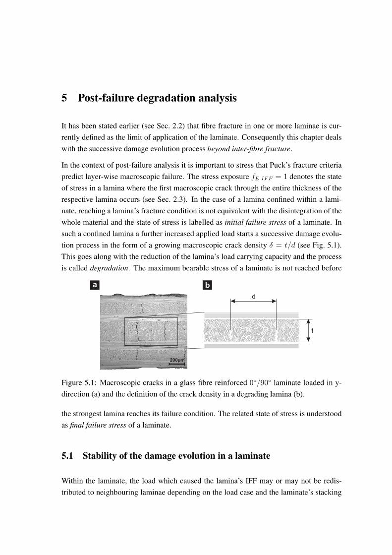
5 Post-failure degradation analysis
It has been stated earlier (see Sec. 2.2) that fibre fracture in one or more laminae is cur-rently defined as the limit of application of the laminate. Consequently this chapter dealswith the successive damage evolution process beyond inter-fibre fracture.
In the context of post-failure analysis it is important to stress that Puck’s fracture criteriapredict layer-wise macroscopic failure. The stress exposure 𝑓𝐸 𝐼𝐹𝐹 = 1 denotes the stateof stress in a lamina where the first macroscopic crack through the entire thickness of therespective lamina occurs (see Sec. 2.3). In the case of a lamina confined within a lami-nate, reaching a lamina’s fracture condition is not equivalent with the disintegration of thewhole material and the state of stress is labelled as initial failure stress of a laminate. Insuch a confined lamina a further increased applied load starts a successive damage evolu-tion process in the form of a growing macroscopic crack density 𝛿 = 𝑡/𝑑 (see Fig. 5.1).This goes along with the reduction of the lamina’s load carrying capacity and the processis called degradation. The maximum bearable stress of a laminate is not reached before
a b
d
t
Figure 5.1: Macroscopic cracks in a glass fibre reinforced 0∘/90∘ laminate loaded in y-direction (a) and the definition of the crack density in a degrading lamina (b).
the strongest lamina reaches its failure condition. The related state of stress is understoodas final failure stress of a laminate.
5.1 Stability of the damage evolution in a laminate
Within the laminate, the load which caused the lamina’s IFF may or may not be redis-tributed to neighbouring laminae depending on the load case and the laminate’s stacking
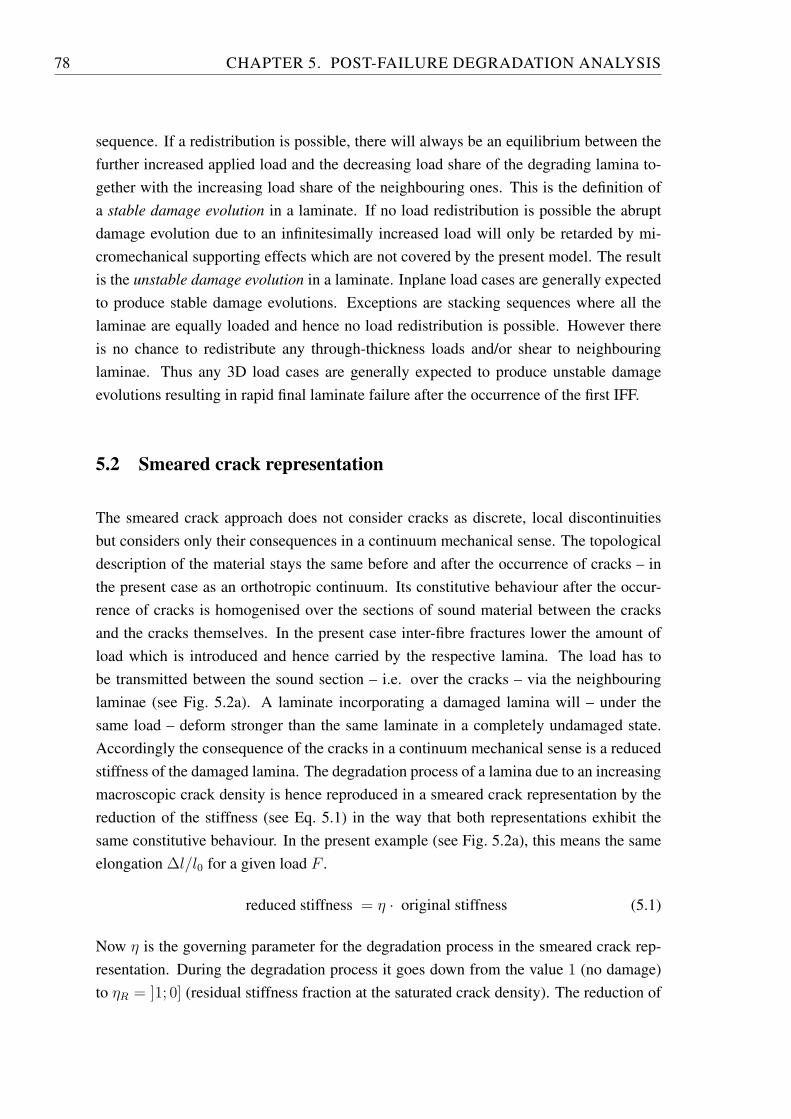
78 CHAPTER 5. POST-FAILURE DEGRADATION ANALYSIS
sequence. If a redistribution is possible, there will always be an equilibrium between thefurther increased applied load and the decreasing load share of the degrading lamina to-gether with the increasing load share of the neighbouring ones. This is the definition ofa stable damage evolution in a laminate. If no load redistribution is possible the abruptdamage evolution due to an infinitesimally increased load will only be retarded by mi-cromechanical supporting effects which are not covered by the present model. The resultis the unstable damage evolution in a laminate. Inplane load cases are generally expectedto produce stable damage evolutions. Exceptions are stacking sequences where all thelaminae are equally loaded and hence no load redistribution is possible. However thereis no chance to redistribute any through-thickness loads and/or shear to neighbouringlaminae. Thus any 3D load cases are generally expected to produce unstable damageevolutions resulting in rapid final laminate failure after the occurrence of the first IFF.
5.2 Smeared crack representation
The smeared crack approach does not consider cracks as discrete, local discontinuitiesbut considers only their consequences in a continuum mechanical sense. The topologicaldescription of the material stays the same before and after the occurrence of cracks – inthe present case as an orthotropic continuum. Its constitutive behaviour after the occur-rence of cracks is homogenised over the sections of sound material between the cracksand the cracks themselves. In the present case inter-fibre fractures lower the amount ofload which is introduced and hence carried by the respective lamina. The load has tobe transmitted between the sound section – i.e. over the cracks – via the neighbouringlaminae (see Fig. 5.2a). A laminate incorporating a damaged lamina will – under thesame load – deform stronger than the same laminate in a completely undamaged state.Accordingly the consequence of the cracks in a continuum mechanical sense is a reducedstiffness of the damaged lamina. The degradation process of a lamina due to an increasingmacroscopic crack density is hence reproduced in a smeared crack representation by thereduction of the stiffness (see Eq. 5.1) in the way that both representations exhibit thesame constitutive behaviour. In the present example (see Fig. 5.2a), this means the sameelongation Δ𝑙/𝑙0 for a given load 𝐹 .
reduced stiffness = 𝜂 ⋅ original stiffness (5.1)
Now 𝜂 is the governing parameter for the degradation process in the smeared crack rep-resentation. During the degradation process it goes down from the value 1 (no damage)to 𝜂𝑅 = ]1; 0] (residual stiffness fraction at the saturated crack density). The reduction of
5.3. EXISTING DEGRADATION PROCEDURES 79
the stiffnesses is then
reduction = 1− 𝜂 (5.2)
and starts from 0 (no damage) and increases up to 1− 𝜂𝑅.
a
b
x
z
90°
0°
90°y
F
FF
F
original stiffness
reduced stiffness
l +l(F)
0 D
flux of force
s m e a r e d c r a c k s
d i s c r e t e c r a c k s
Figure 5.2: Discrete crack (a) and smeared crack representation (b) of a confined degrad-ing lamina.
There are numerous approaches to correlate the density, form, size and position of crackswith their effects on the stiffness [93], but the following degradation rules are exclusivelydefined in the smeared crack representation of the degrading lamina. Hence it is importantfor the development and validation1 to keep in mind that the degradation process is agrowth of crack density in reality, but neither the actual value of the crack density 𝛿 norpossible correlations between the discrete and smeared crack representation do play a rolein this work.
5.3 Existing degradation procedures
It is obvious, that the amount of load beyond the IFF, the thereby generated crack densityand the according degradation parameter 𝜂 of the smeared crack representation are tobe correlated to define a valid material behaviour for a post-failure degradation analysis.Keeping strictly inside the smeared crack representation, the detour via the crack densitymay be omitted and the correlation between the amount of load beyond the IFF and thedegradation parameter 𝜂 or the resulting reduced stiffnesses is the remaining task of anydegradation rule.
1Does the model meet the reality?
80 CHAPTER 5. POST-FAILURE DEGRADATION ANALYSIS
5.3.1 Excessive IFF stress exposure
Early experiments with laminates loaded inplane (𝜎𝑦 and/or 𝜏𝑥𝑦) beyond IFF [39] led toan empirical correlation between the applied load beyond the IFF and the degradationparameter 𝜂 via the IFF stress exposure persistently calculated with original stiffnesses(see Eq. 5.3). Calculating 𝑓𝐸 𝐼𝐹𝐹 with the unchanged original stiffnesses results in values𝑓𝐸 𝐼𝐹𝐹 > 1 for load cases beyond an IFF.
𝜂 (𝑓𝐸 𝐼𝐹𝐹 ) =1− 𝜂𝑅
1 + 𝑎 (𝑓𝐸 𝐼𝐹𝐹 − 1)𝜁+ 𝜂𝑅 for 𝑓𝐸 𝐼𝐹𝐹 > 1 (5.3)
The definition (Eq. 5.3) results in 𝜂 = 1 for the onset of damage (𝑓𝐸 𝐼𝐹𝐹 = 1) andconverges against the residual stiffness fraction 𝜂𝑅 at the saturated crack density for𝑓𝐸 𝐼𝐹𝐹 → ∞. Loading a laminate inplane, the laminae are subjected to transverse stress𝜎2 and inplane shear stress 𝜏12 only. Hence only the transverse Young’s modulus 𝐸2 andthe inplane shear modulus 𝐺12 are available for degradation (see Eq. 5.4). It is obvi-ous, that IFFs continue to transmit pressure 𝜎𝑛 < 0 over the crack edges hence there isno reduction of the respective stiffness in these cases. In the early development stagesalso the Poisson’s ratios were degraded but later experiments strongly suggested keepingthem constant [94]. Accordingly no Poisson’s ratio degradation is specified throughoutthe present work.
𝐸𝑟𝑒𝑑2 =
⎧⎨⎩𝜂 ⋅ 𝐸𝑜𝑟𝑖𝑔2 for tensile 𝜎𝑛 on the fracture plane
𝐸𝑜𝑟𝑖𝑔2 for compressive 𝜎𝑛 on the fracture plane
(5.4)
𝐺𝑟𝑒𝑑12 = 𝜂 ⋅𝐺𝑜𝑟𝑖𝑔
12
The mentioned original stiffnesses (index orig) which are used to calculate the exceededIFF stress exposure are the secant moduli at the IFF limit, thus the last valid secant moduliin the case of a nonlinear constitutive material model (see Sec. 3.1.2).
Further experiments [95, 96] have revealed that reasonable parameters for equation 5.3are 𝑎 = [0.95; 5.5] and 𝜁 = [1.17; 1.5] depending on the material. These studies alsosuggest to reduce 𝐺12 less than 𝐸2. Using the excessive IFF stress exposure approach thisis implemented in equation 5.3 by different residual stiffness fractions 𝜂𝑅𝐸
= 0.03 and𝜂𝑅𝐺
= 0.25 for GFRC or 𝜂𝑅𝐺= 0.6 for CFRC [88]. The suggested values are equivalent
with the reduction of 𝐺12 by only 𝑘 = 77% for CFRC and 𝑘 = 41% for GFRC of thereduction of 𝐸2:
𝐸𝑟𝑒𝑑2 =
⎧⎨⎩𝐸𝑜𝑟𝑖𝑔2 ⋅ (1− reduction) for tensile 𝜎𝑛 on the fracture plane
𝐸𝑜𝑟𝑖𝑔2 for compressive 𝜎𝑛 on the fracture plane
(5.5)
𝐺𝑟𝑒𝑑12 = 𝐺𝑜𝑟𝑖𝑔
12 ⋅ (1− 𝑘 ⋅ reduction)
5.3. EXISTING DEGRADATION PROCEDURES 81
It has been stated in earlier works that the approach has proven its applicability on a widerange of materials and stacking sequences [4, 94]. However aiming on a completely 3Dfailure and post-failure analysis, this approach is judged as strictly limited to inplane loadcases without the potential of being extended to 3D load cases. The approach completelyneglects that a stable damage evolution process requires and is governed by a load re-distribution process. In the case of loads or stacking sequences leading to an unstabledamage evolution process or even for an isolated single lamina, the excessive IFF stressexposure approach predicts an unrealistic, smooth degradation process of the damaginglaminae. The application of this method is restricted to the analysis of doubtlessly stabledamage evolution processes under inplane load.
Validity check
Puck’s Theory is a stress-based, layer-wise fracture criterion, it defines the maximumbearable stress state in a lamina. Increasing the applied load beyond IFF there is noreason why the laminate should be able to bear more stress, in fact it partly gets rid of itsload by a redistribution in the process of the reduction of stiffnesses and the associatedincrease of strain. A degradation procedure which plausibly predicts this process enablesto associate any given state of strain in a lamina (beyond IFF) with the transmitted loadby the lamina or the state of stress in the smeared crack representation of the lamina,respectively. However the procedure may not define a state of strain for an arbitrary highamount of stress, because the stress-based fracture criterion defines a stress threshold,beyond which the states of stress are just not bearable.
Applying the excessive IFF stress exposure approach to any given state of strain beyondIFF, the original stiffnesses provide a state of stress based on which the IFF stress ex-posure takes a value of 𝑓𝐸 𝐼𝐹𝐹 > 1. Equation 5.3 leads to a value of 𝜂 = ]1; 𝜂𝑅] andequation 5.5 provides the reduced stiffnesses of the degrading lamina. The application ofthese stiffnesses to the given state of strain leads to the associated state of stress in thesmeared crack representation of the degrading lamina. The excessive IFF stress exposureapproach also permits to assign a state of strain to any given state of stress beyond IFF.At a given state of stress beyond IFF, the IFF stress exposure takes a value of 𝑓𝐸 𝐼𝐹𝐹 > 1,equation 5.3 leads to a value of 𝜂 = ]1; 𝜂𝑅] and equation 5.5 offers the reduced stiffnesses.Applying these stiffnesses to the given state of stress leads to the associated state of strainin the smeared crack representation of the degrading lamina. This result is completelyunphysical and does not qualify the presented approach for a general application.
82 CHAPTER 5. POST-FAILURE DEGRADATION ANALYSIS
5.3.2 Constant IFF stress exposure
The constant IFF stress exposure approach overcomes the purely empirical nature of theapproach above and is based on physical and mechanical considerations [5, 6]. The ap-proach conserves the meaning of the value 𝑓𝐸 𝐼𝐹𝐹 = 1 as a fracture criterion and isin accordance with degradation procedures based on different failure criteria which alsopostulate the failure criterion to be the degradation governing measure [97]. There is noconceivable situation in which a sound lamina experiences an IFF stress exposure above1. When the stress exposure of a lamina reaches this value an IFF occurs and therewiththe lamina gets rid of parts of its load by a redistribution or all of its load by separation,respectively. In reverse the density of cracks emerging due to an increasing load beyondthe IFF permanently adjusts to that value at which the IFF stress exposure threshold of𝑓𝐸 𝐼𝐹𝐹 = 1 is not exceeded. This means for the degradation process of a lamina, that– at a given state of strain beyond IFF – the degradation parameter 𝜂 takes exactly thatvalue, for which the the resulting stresses generate an IFF stress exposure of 1. There isno longer an analytical degradation rule like equation 5.3 but the amount of degradationis defined by the threshold
𝑓𝐸 𝐼𝐹𝐹 = 1 = constant . (5.6)
For inplane load cases, the impact of the degradation on the respective stiffnesses definedin equation 5.5 stays valid but the residual stiffnesses are no longer accounted for by resid-ual stiffness fractions 𝜂𝑅. Now the impact of the degradation process on the respectivestiffness is stopped when it has reached its experimentally determined residual stiffnessvalue. The degradation process in the respective lamina is completed when – after a sta-ble damage evolution process – a valid solution for 𝜂 can no longer be found. This is thecase after all the relevant stiffnesses have already been degraded down to their residualstiffness values.
The approach meets the requirements of the validity check above (see Sec. 5.3.1). For anygiven state of strain beyond the IFF the original stiffnesses result in 𝑓𝐸 𝐼𝐹𝐹 > 1 but therewill generally be a value of 𝜂 which reduces the stiffnesses and hence the stresses down tothe state where 𝑓𝐸 𝐼𝐹𝐹 = 1. For any given state of stress beyond the IFF there will be novalue of 𝜂 within its domain of definition [1; 0] which is able to generate 𝑓𝐸 𝐼𝐹𝐹 = 1. As aresult the approach does not provide a valid solution for unstable damage evolution wherethe stresses in the laminae inevitably rise with an increasingly applied load beyond IFF.Accordingly the approach is capable of identifying unstable damage evolution processes.The approach has proven its capability and reliability in the WWFE-I inplane load cases[5, 6] and it is implemented in the material subroutines in the present work (see Ch. 6). Inthe course of the application there were however identified two problems of the method:
5.3. EXISTING DEGRADATION PROCEDURES 83
Degradation locking in the case of fibre-perpendicular compression
Using equation 5.5 for the definition of the impact of the degradation on the respectivestiffnesses results in no valid solution for 𝜂 in the case of fibre-perpendicular compressionalthough compression in the y-direction might result in a stable damage evolution processup to a certain point. Experimental experience however suggests, that inclined IFFs dueto inplane compression in the respective lamina (Modus C fractures, see Sec. 4.2.4) definethe limit of use of the laminate (see Sec. 2.3). The amount of load beyond the IFF, whichcan be transmitted over the crack edges before the wedge effect leads to a sudden disin-tegration of the laminate, is currently unpredictable. Accordingly such IFFs are classifiedas non-tolerable fractures and no post-failure degradation analysis is started after suchfractures. There are currently no experimental results concerning the damage evolutionin a laminate subjected to compression in the z-direction. This kind of applied load isexpected to result in a crushing of the damaging lamina which is a mechanism far beyondthe capabilities of a continuum based smeared crack representation. Within the presentwork aiming on macroscopic and physical (in contrast to empirical) material descriptionssuch post-failure behaviour is classified as currently unpredictable.
Lack of adjustability to experimental results
Although the extremely limited availability of experimental degradation process data,the lack of adjustability of the constant IFF stress exposure approach is identified as adrawback. This becomes even more evident if the following theoretical aspect is con-sidered: The applied threshold for the occurrence of further inter-fibre fractures duringthe degradation process 𝑓𝐸 𝐼𝐹𝐹 = 1 is defined in the smeared crack representation of thedamaging lamina, but the actual crack presumably emerges in the centre of a sound sec-tion of the lamina between two discrete cracks (see Fig. 5.2). Predicting fractures in thesound sections of the discrete crack representation with a criterion based on the smearedcrack representation implies identical states of stress in both of them. Comprehending thederivation of the reduced stiffnesses of the smeared crack representation (see Sec. 5.6.1)identifies the approach above to be based on a reasonable but simplifying assumption.Without further experimental or numerical investigations 𝑓𝐸 𝐼𝐹𝐹 = 1 = constant is anacceptable degradation approach, but the enhancement described below (see Sec. 5.4)prepares the degradation rule for future findings.
84 CHAPTER 5. POST-FAILURE DEGRADATION ANALYSIS
5.4 Variable IFF stress exposure
The degradation rule described above (see Sec. 5.3.2) becomes adjustable to experimen-tal findings if the threshold IFF stress exposure 𝑓𝐸 𝐼𝐹𝐹 , at which new inter-fibre fracturesemerge, is not constantly 1 but depends on the progress in the degradation process [98].As the central degradation parameter is 𝜂, a linear dependence of 𝑓 𝑟𝑒𝑑𝐸 𝐼𝐹𝐹 (𝜂) is a straight-forward ansatz. Now the degradation process has not only an impact on the stiffnessesaccording to equation 5.5 but also on the bearable stress exposure of the lamina:
𝑓 𝑟𝑒𝑑𝐸 𝐼𝐹𝐹 = 𝑓 𝑜𝑟𝑖𝑔𝐸 𝐼𝐹𝐹 ⋅ (1− 𝑙 ⋅ reduction) = 1− 𝑙 ⋅ reduction (5.7)
Latest experiments suggest the bearable IFF stress exposure to decline in the course of thedegradation process. This finding is in accordance with theoretical aspects arising fromthe smeared crack representation (see Secs. 5.2 and 5.6.1, particular Eq. 5.13). Howeverit has to be assured that the involved stiffnesses decline faster that the bearable stressexposure – otherwise no valid solution for 𝜂 can be found. Without further experimentsthe range for the impact factor 𝑙 is theoretically limited to ]0; 𝑘[ for inplane load casesbut more detailed information is currently not available. The question whether there is aresidual bearable IFF stress exposure or not is currently unanswered. Hence the variableIFF stress exposure approach is not implemented in the material subroutines in the presentwork (see Ch. 6).
5.5 3D degradation procedure
The existing degradation procedures have been developed, validated and calibrated forinplane load cases. The aim of providing a comprehensive failure prediction for UD fibre-reinforced laminates with complex geometries and under 3D load (see Ch. 1) requires thedevelopment of a 3D post-failure degradation analysis even if it has been stated, thatthrough-thickness load and/or shear will in the majority of cases lead to unstable damageevolution processes (see Sec. 5.1). The desired output of a 3D degradation analysis willeither be
∘ the reliable information that an unstable damage evolution process starts when ex-ceeding the IFF criterion,
∘ or the 3D constitutive behaviour of a degrading lamina at any state of a stable dam-age evolution process.
5.5. 3D DEGRADATION PROCEDURE 85
If only the stable damage evolution process is to be analysed it is sufficient to definethose reduced stiffnesses, which influence the load redistribution process. If the structurefulfils multiple purposes or is subjected to cyclic load (see Sec. 2.4) it is furthermoreimportant to know how the damaged structure behaves under a general load case which isdifferent from the one which produced the damage. This analysis task requires the full 3Dconstitutive behaviour of the damaging lamina at any state during its degradation process.
The previous sections have outlined that a degradation procedure consists of two defini-tions:
∘ The definition, how far a degradation process progresses due to an applied loadbeyond IFF (see Eqs. 5.3, 5.6 or 5.7):The application of the excessive IFF stress exposure approach disqualifies for the3D case due to its disability to identify unstable damage evolution. The variable IFFstress exposure approach is not even experimentally confirmed for inplane cases,hence the constant IFF stress exposure approach is chosen to be the governing rulefor the 3D degradation procedure.
∘ The definition of the impact of the degradation process on the involved measures(see Eqs. 5.4, 5.5 or 5.7):In the 3D case there are significantly more stiffnesses available for a degradationbeyond IFF – 𝐸2, 𝐸3, 𝐺12, 𝐺13 and 𝐺23. The impact of the degradation processon the respective stiffness is depending on the orientation of the IFF fracture plane𝜃𝑓𝑝. Existing considerations on these dependencies [76] have turned out to be in-complete but are the basis for the described development of the approach.
For the development of a fracture angle-dependent degradation rule the relevant questionis, which fracture plane orientation degrades which stiffness to which amount. The inves-tigation is expected to be more efficient if the question is changed to:Which are the two fracture plane orientations which have the most direct and the leastimpact on the load bearing capacity of a lamina against the respective types of load?The results are regarded to be transferable to the impact of the fracture plane orientationon the degradation of the associated stiffnesses one-to-one. It has been stated earlier thattension and compression are affected unequally by the degradation hence positive andnegative loads are treated separately. Regarding transverse tension (see Fig. 5.3) a frac-ture plane orientation of 𝜃𝑓𝑝 = 0∘ is expected to have the most direct impact on the loadbearing capacity whereas a fracture at 𝜃𝑓𝑝 = 90∘ has no influence. In the case of through-thickness tension it is vice versa and in the compressive cases no impact of any fractureplane orientation on the respectice load bearing capacity is determinable.
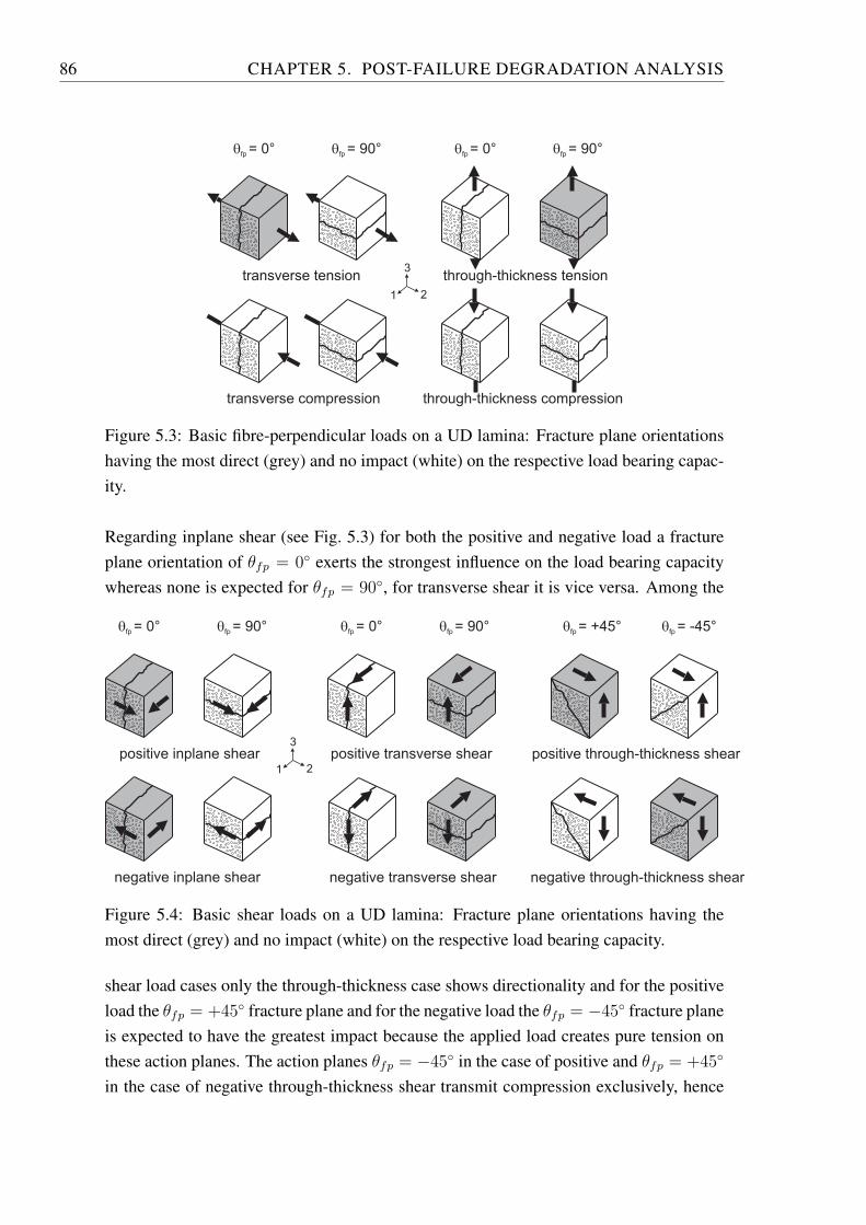
86 CHAPTER 5. POST-FAILURE DEGRADATION ANALYSIS
1
3
2
through-thickness compression
through-thickness tension
transverse compression
transverse tension
qfp = 0° qfp = 90° qfp = 0° qfp = 90°
Figure 5.3: Basic fibre-perpendicular loads on a UD lamina: Fracture plane orientationshaving the most direct (grey) and no impact (white) on the respective load bearing capac-ity.
Regarding inplane shear (see Fig. 5.3) for both the positive and negative load a fractureplane orientation of 𝜃𝑓𝑝 = 0∘ exerts the strongest influence on the load bearing capacitywhereas none is expected for 𝜃𝑓𝑝 = 90∘, for transverse shear it is vice versa. Among the
positive inplane shear
negative inplane shear
positive transverse shear
negative transverse shear
positive through-thickness shear
negative through-thickness shear
qfp = 0° qfp = 90° qfp = +45° qfp = -45°qfp = 0° qfp = 90°
1
3
2
Figure 5.4: Basic shear loads on a UD lamina: Fracture plane orientations having themost direct (grey) and no impact (white) on the respective load bearing capacity.
shear load cases only the through-thickness case shows directionality and for the positiveload the 𝜃𝑓𝑝 = +45∘ fracture plane and for the negative load the 𝜃𝑓𝑝 = −45∘ fracture planeis expected to have the greatest impact because the applied load creates pure tension onthese action planes. The action planes 𝜃𝑓𝑝 = −45∘ in the case of positive and 𝜃𝑓𝑝 = +45∘
in the case of negative through-thickness shear transmit compression exclusively, hence
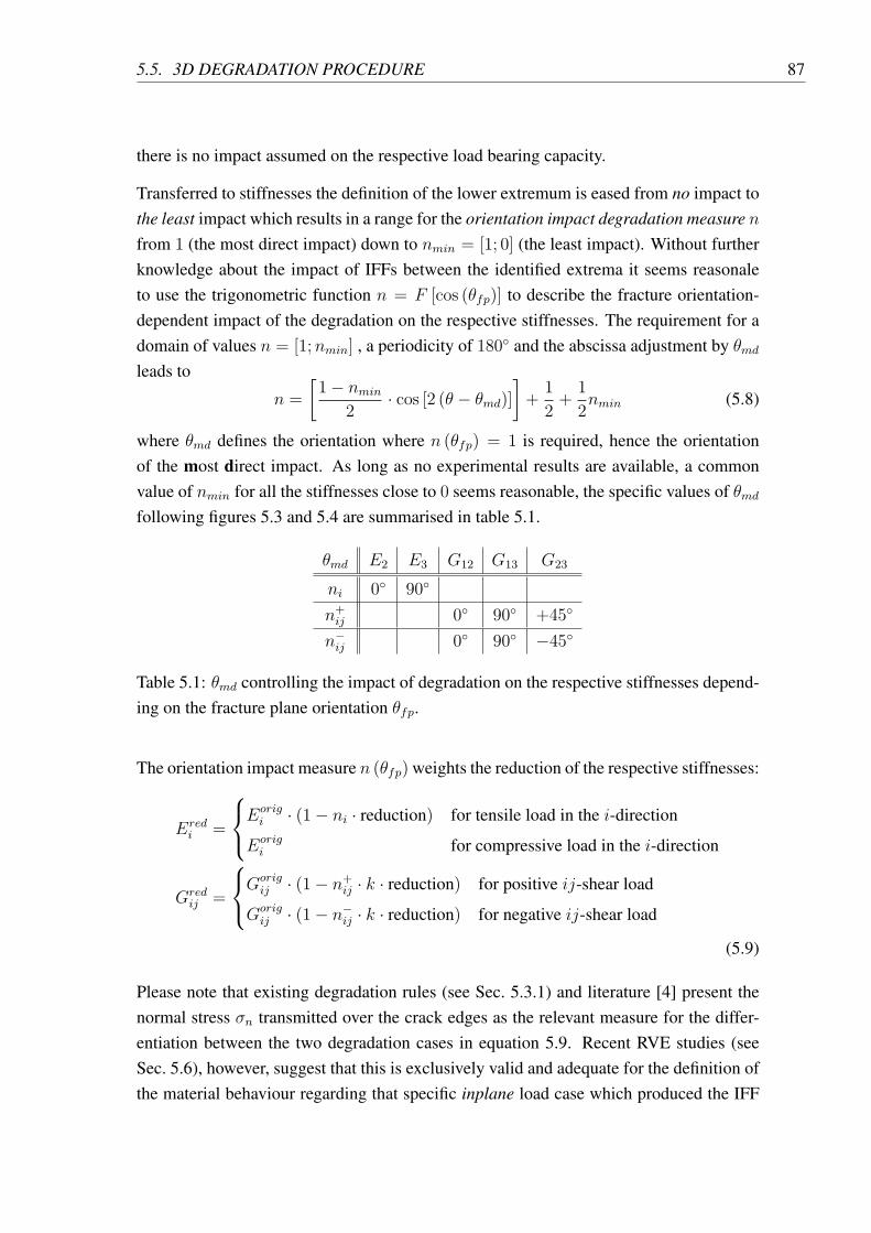
5.5. 3D DEGRADATION PROCEDURE 87
there is no impact assumed on the respective load bearing capacity.
Transferred to stiffnesses the definition of the lower extremum is eased from no impact tothe least impact which results in a range for the orientation impact degradation measure 𝑛from 1 (the most direct impact) down to 𝑛𝑚𝑖𝑛 = [1; 0] (the least impact). Without furtherknowledge about the impact of IFFs between the identified extrema it seems reasonaleto use the trigonometric function 𝑛 = 𝐹 [cos (𝜃𝑓𝑝)] to describe the fracture orientation-dependent impact of the degradation on the respective stiffnesses. The requirement for adomain of values 𝑛 = [1;𝑛𝑚𝑖𝑛] , a periodicity of 180∘ and the abscissa adjustment by 𝜃𝑚𝑑leads to
𝑛 =
[1− 𝑛𝑚𝑖𝑛
2⋅ cos [2 (𝜃 − 𝜃𝑚𝑑)]
]+
1
2+
1
2𝑛𝑚𝑖𝑛 (5.8)
where 𝜃𝑚𝑑 defines the orientation where 𝑛 (𝜃𝑓𝑝) = 1 is required, hence the orientationof the most direct impact. As long as no experimental results are available, a commonvalue of 𝑛𝑚𝑖𝑛 for all the stiffnesses close to 0 seems reasonable, the specific values of 𝜃𝑚𝑑following figures 5.3 and 5.4 are summarised in table 5.1.
𝜃𝑚𝑑 𝐸2 𝐸3 𝐺12 𝐺13 𝐺23
𝑛𝑖 0∘ 90∘
𝑛+𝑖𝑗 0∘ 90∘ +45∘
𝑛−𝑖𝑗 0∘ 90∘ −45∘
Table 5.1: 𝜃𝑚𝑑 controlling the impact of degradation on the respective stiffnesses depend-ing on the fracture plane orientation 𝜃𝑓𝑝.
The orientation impact measure 𝑛 (𝜃𝑓𝑝) weights the reduction of the respective stiffnesses:
𝐸𝑟𝑒𝑑𝑖 =
⎧⎨⎩𝐸𝑜𝑟𝑖𝑔𝑖 ⋅ (1− 𝑛𝑖 ⋅ reduction) for tensile load in the 𝑖-direction
𝐸𝑜𝑟𝑖𝑔𝑖 for compressive load in the 𝑖-direction
𝐺𝑟𝑒𝑑𝑖𝑗 =
⎧⎨⎩𝐺𝑜𝑟𝑖𝑔𝑖𝑗 ⋅ (1− 𝑛+
𝑖𝑗 ⋅ 𝑘 ⋅ reduction) for positive 𝑖𝑗-shear load
𝐺𝑜𝑟𝑖𝑔𝑖𝑗 ⋅ (1− 𝑛−
𝑖𝑗 ⋅ 𝑘 ⋅ reduction) for negative 𝑖𝑗-shear load
(5.9)
Please note that existing degradation rules (see Sec. 5.3.1) and literature [4] present thenormal stress 𝜎𝑛 transmitted over the crack edges as the relevant measure for the differ-entiation between the two degradation cases in equation 5.9. Recent RVE studies (seeSec. 5.6), however, suggest that this is exclusively valid and adequate for the definition ofthe material behaviour regarding that specific inplane load case which produced the IFF
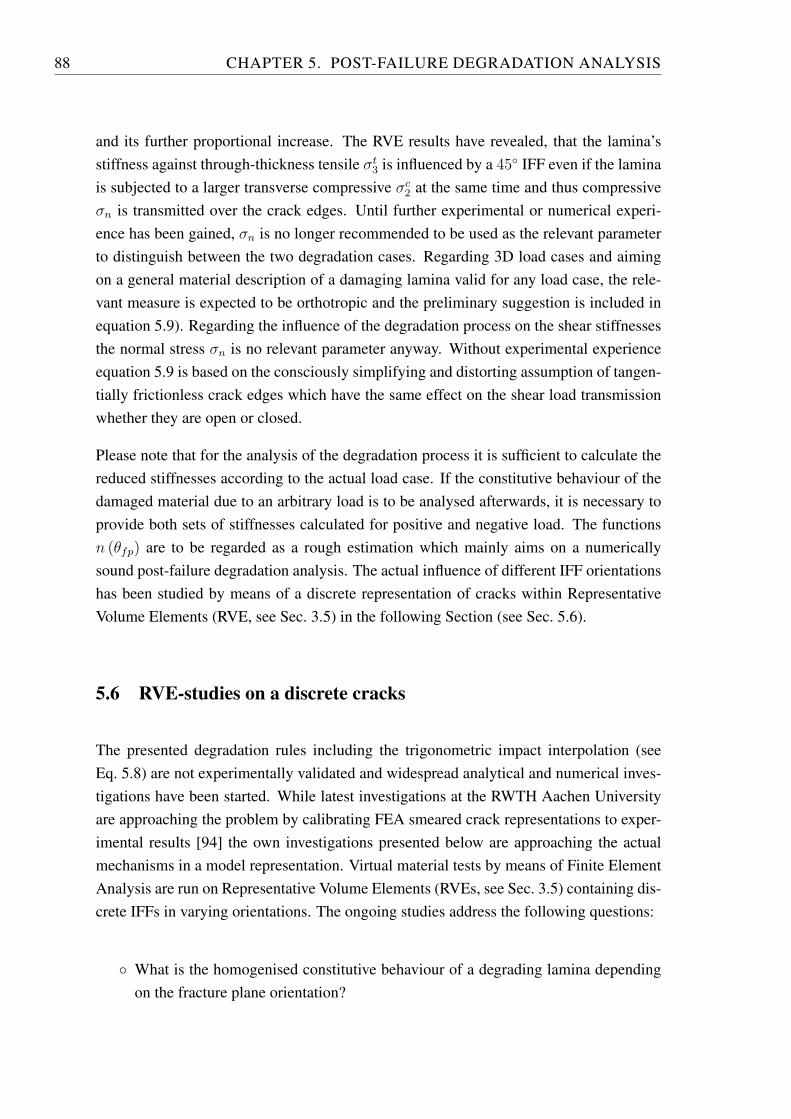
88 CHAPTER 5. POST-FAILURE DEGRADATION ANALYSIS
and its further proportional increase. The RVE results have revealed, that the lamina’sstiffness against through-thickness tensile 𝜎𝑡3 is influenced by a 45∘ IFF even if the laminais subjected to a larger transverse compressive 𝜎𝑐2 at the same time and thus compressive𝜎𝑛 is transmitted over the crack edges. Until further experimental or numerical experi-ence has been gained, 𝜎𝑛 is no longer recommended to be used as the relevant parameterto distinguish between the two degradation cases. Regarding 3D load cases and aimingon a general material description of a damaging lamina valid for any load case, the rele-vant measure is expected to be orthotropic and the preliminary suggestion is included inequation 5.9). Regarding the influence of the degradation process on the shear stiffnessesthe normal stress 𝜎𝑛 is no relevant parameter anyway. Without experimental experienceequation 5.9 is based on the consciously simplifying and distorting assumption of tangen-tially frictionless crack edges which have the same effect on the shear load transmissionwhether they are open or closed.
Please note that for the analysis of the degradation process it is sufficient to calculate thereduced stiffnesses according to the actual load case. If the constitutive behaviour of thedamaged material due to an arbitrary load is to be analysed afterwards, it is necessary toprovide both sets of stiffnesses calculated for positive and negative load. The functions𝑛 (𝜃𝑓𝑝) are to be regarded as a rough estimation which mainly aims on a numericallysound post-failure degradation analysis. The actual influence of different IFF orientationshas been studied by means of a discrete representation of cracks within RepresentativeVolume Elements (RVE, see Sec. 3.5) in the following Section (see Sec. 5.6).
5.6 RVE-studies on a discrete cracks
The presented degradation rules including the trigonometric impact interpolation (seeEq. 5.8) are not experimentally validated and widespread analytical and numerical inves-tigations have been started. While latest investigations at the RWTH Aachen Universityare approaching the problem by calibrating FEA smeared crack representations to exper-imental results [94] the own investigations presented below are approaching the actualmechanisms in a model representation. Virtual material tests by means of Finite ElementAnalysis are run on Representative Volume Elements (RVEs, see Sec. 3.5) containing dis-crete IFFs in varying orientations. The ongoing studies address the following questions:
∘ What is the homogenised constitutive behaviour of a degrading lamina dependingon the fracture plane orientation?
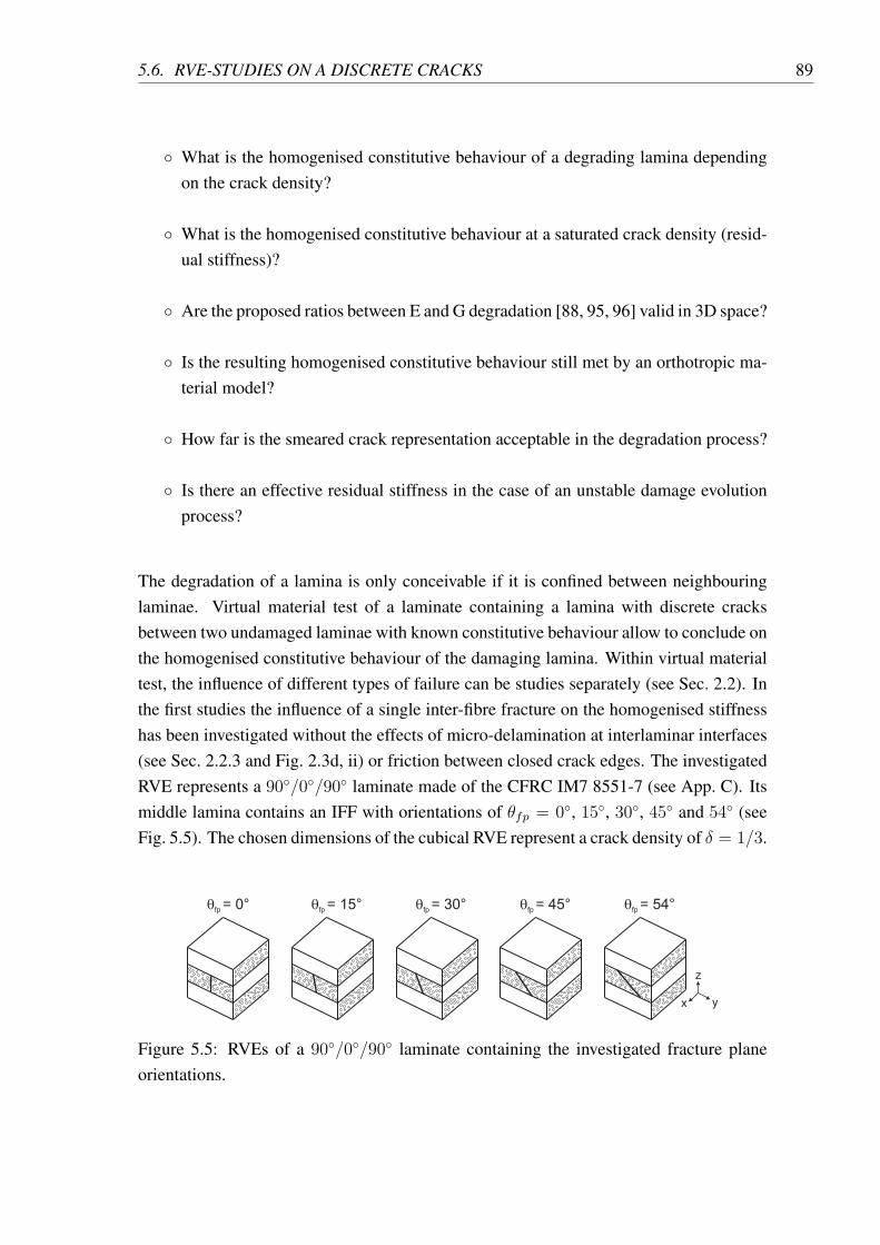
5.6. RVE-STUDIES ON A DISCRETE CRACKS 89
∘ What is the homogenised constitutive behaviour of a degrading lamina dependingon the crack density?
∘ What is the homogenised constitutive behaviour at a saturated crack density (resid-ual stiffness)?
∘ Are the proposed ratios between E and G degradation [88, 95, 96] valid in 3D space?
∘ Is the resulting homogenised constitutive behaviour still met by an orthotropic ma-terial model?
∘ How far is the smeared crack representation acceptable in the degradation process?
∘ Is there an effective residual stiffness in the case of an unstable damage evolutionprocess?
The degradation of a lamina is only conceivable if it is confined between neighbouringlaminae. Virtual material test of a laminate containing a lamina with discrete cracksbetween two undamaged laminae with known constitutive behaviour allow to conclude onthe homogenised constitutive behaviour of the damaging lamina. Within virtual materialtest, the influence of different types of failure can be studies separately (see Sec. 2.2). Inthe first studies the influence of a single inter-fibre fracture on the homogenised stiffnesshas been investigated without the effects of micro-delamination at interlaminar interfaces(see Sec. 2.2.3 and Fig. 2.3d, ii) or friction between closed crack edges. The investigatedRVE represents a 90∘/0∘/90∘ laminate made of the CFRC IM7 8551-7 (see App. C). Itsmiddle lamina contains an IFF with orientations of 𝜃𝑓𝑝 = 0∘, 15∘, 30∘, 45∘ and 54∘ (seeFig. 5.5). The chosen dimensions of the cubical RVE represent a crack density of 𝛿 = 1/3.
x
z
y
qfp = 0° qfp = 15° qfp = 30° qfp = 45° qfp = 54°
Figure 5.5: RVEs of a 90∘/0∘/90∘ laminate containing the investigated fracture planeorientations.
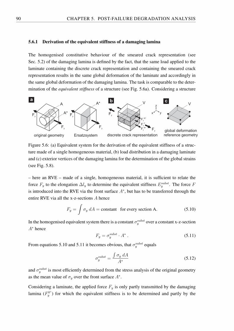
90 CHAPTER 5. POST-FAILURE DEGRADATION ANALYSIS
5.6.1 Derivation of the equivalent stiffness of a damaging lamina
The homogenised constitutive behaviour of the smeared crack representation (seeSec. 5.2) of the damaging lamina is defined by the fact, that the same load applied to thelaminate containing the discrete crack representation and containing the smeared crackrepresentation results in the same global deformation of the laminate and accordingly inthe same global deformation of the damaging lamina. The task is comparable to the deter-mination of the equivalent stiffness of a structure (see Fig. 5.6a). Considering a structure
x
z
y
Fy
Fy
A*
Fy
Fy
A
Fy
Fy
A*
original geometry Ersatzsystem discrete crack representation
a b
global deformationreference geometry
c
Fy
0°
Fy
90°
Fy
90°
V V
Figure 5.6: (a) Equivalent system for the derivation of the equivalent stiffness of a struc-ture made of a single homogeneous material, (b) load distribution in a damaging laminateand (c) exterior vertices of the damaging lamina for the determination of the global strains(see Fig. 5.8).
– here an RVE – made of a single, homogeneous material, it is sufficient to relate theforce 𝐹𝑦 to the elongation Δ𝑙𝑦 to determine the equivalent stiffness 𝐸𝑠𝑢𝑏𝑠𝑡
𝑦 . The force 𝐹is introduced into the RVE via the front surface 𝐴∗, but has to be transferred through theentire RVE via all the x-z-sections 𝐴 hence
𝐹𝑦 =
∫𝜎𝑦 𝑑𝐴 = constant for every section A. (5.10)
In the homogenised equivalent system there is a constant 𝜎𝑠𝑢𝑏𝑠𝑡𝑦 over a constant x-z-section𝐴∗ hence
𝐹𝑦 = 𝜎𝑠𝑢𝑏𝑠𝑡𝑦 ⋅ 𝐴∗ . (5.11)
From equations 5.10 and 5.11 it becomes obvious, that 𝜎𝑠𝑢𝑏𝑠𝑡𝑦 equals
𝜎𝑠𝑢𝑏𝑠𝑡𝑦 =
∫𝜎𝑦 𝑑𝐴
𝐴∗ (5.12)
and 𝜎𝑠𝑢𝑏𝑠𝑡𝑦 is most efficiently determined from the stress analysis of the original geometryas the mean value of 𝜎𝑦 over the front surface 𝐴∗.
Considering a laminate, the applied force 𝐹𝑦 is only partly transmitted by the damaginglamina (𝐹 0∘
𝑦 ) for which the equivalent stiffness is to be determined and partly by the
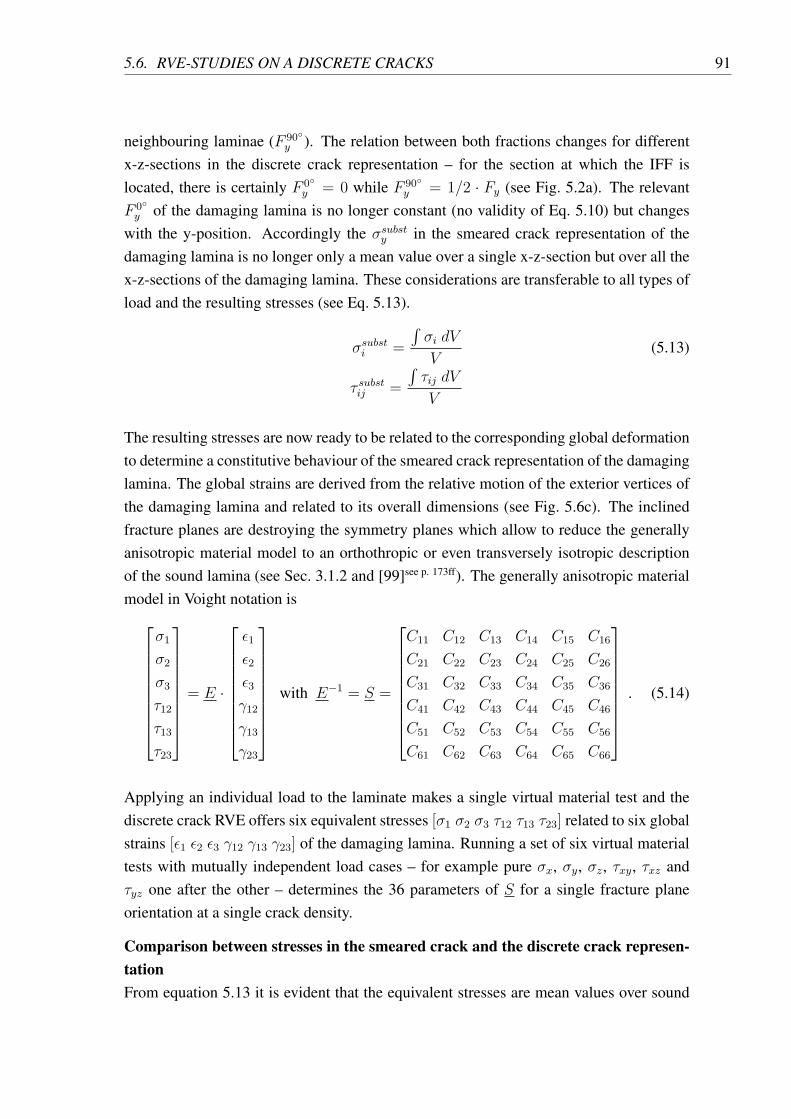
5.6. RVE-STUDIES ON A DISCRETE CRACKS 91
neighbouring laminae (𝐹 90∘𝑦 ). The relation between both fractions changes for different
x-z-sections in the discrete crack representation – for the section at which the IFF islocated, there is certainly 𝐹 0∘
𝑦 = 0 while 𝐹 90∘𝑦 = 1/2 ⋅ 𝐹𝑦 (see Fig. 5.2a). The relevant
𝐹 0∘𝑦 of the damaging lamina is no longer constant (no validity of Eq. 5.10) but changes
with the y-position. Accordingly the 𝜎𝑠𝑢𝑏𝑠𝑡𝑦 in the smeared crack representation of thedamaging lamina is no longer only a mean value over a single x-z-section but over all thex-z-sections of the damaging lamina. These considerations are transferable to all types ofload and the resulting stresses (see Eq. 5.13).
𝜎𝑠𝑢𝑏𝑠𝑡𝑖 =
∫𝜎𝑖 𝑑𝑉
𝑉(5.13)
𝜏 𝑠𝑢𝑏𝑠𝑡𝑖𝑗 =
∫𝜏𝑖𝑗 𝑑𝑉
𝑉
The resulting stresses are now ready to be related to the corresponding global deformationto determine a constitutive behaviour of the smeared crack representation of the damaginglamina. The global strains are derived from the relative motion of the exterior vertices ofthe damaging lamina and related to its overall dimensions (see Fig. 5.6c). The inclinedfracture planes are destroying the symmetry planes which allow to reduce the generallyanisotropic material model to an orthothropic or even transversely isotropic descriptionof the sound lamina (see Sec. 3.1.2 and [99]see p. 173ff). The generally anisotropic materialmodel in Voight notation is⎡⎢⎢⎢⎢⎢⎢⎢⎢⎣
𝜎1
𝜎2
𝜎3
𝜏12
𝜏13
𝜏23
⎤⎥⎥⎥⎥⎥⎥⎥⎥⎦= 𝐸 ⋅
⎡⎢⎢⎢⎢⎢⎢⎢⎢⎣
𝜖1
𝜖2
𝜖3
𝛾12
𝛾13
𝛾23
⎤⎥⎥⎥⎥⎥⎥⎥⎥⎦with 𝐸−1 = 𝑆 =
⎡⎢⎢⎢⎢⎢⎢⎢⎢⎣
𝐶11 𝐶12 𝐶13 𝐶14 𝐶15 𝐶16
𝐶21 𝐶22 𝐶23 𝐶24 𝐶25 𝐶26
𝐶31 𝐶32 𝐶33 𝐶34 𝐶35 𝐶36
𝐶41 𝐶42 𝐶43 𝐶44 𝐶45 𝐶46
𝐶51 𝐶52 𝐶53 𝐶54 𝐶55 𝐶56
𝐶61 𝐶62 𝐶63 𝐶64 𝐶65 𝐶66
⎤⎥⎥⎥⎥⎥⎥⎥⎥⎦. (5.14)
Applying an individual load to the laminate makes a single virtual material test and thediscrete crack RVE offers six equivalent stresses [𝜎1 𝜎2 𝜎3 𝜏12 𝜏13 𝜏23] related to six globalstrains [𝜖1 𝜖2 𝜖3 𝛾12 𝛾13 𝛾23] of the damaging lamina. Running a set of six virtual materialtests with mutually independent load cases – for example pure 𝜎𝑥, 𝜎𝑦, 𝜎𝑧, 𝜏𝑥𝑦, 𝜏𝑥𝑧 and𝜏𝑦𝑧 one after the other – determines the 36 parameters of 𝑆 for a single fracture planeorientation at a single crack density.
Comparison between stresses in the smeared crack and the discrete crack represen-tationFrom equation 5.13 it is evident that the equivalent stresses are mean values over sound
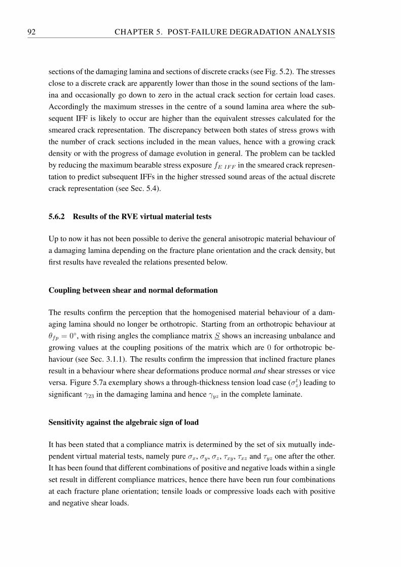
92 CHAPTER 5. POST-FAILURE DEGRADATION ANALYSIS
sections of the damaging lamina and sections of discrete cracks (see Fig. 5.2). The stressesclose to a discrete crack are apparently lower than those in the sound sections of the lam-ina and occasionally go down to zero in the actual crack section for certain load cases.Accordingly the maximum stresses in the centre of a sound lamina area where the sub-sequent IFF is likely to occur are higher than the equivalent stresses calculated for thesmeared crack representation. The discrepancy between both states of stress grows withthe number of crack sections included in the mean values, hence with a growing crackdensity or with the progress of damage evolution in general. The problem can be tackledby reducing the maximum bearable stress exposure 𝑓𝐸 𝐼𝐹𝐹 in the smeared crack represen-tation to predict subsequent IFFs in the higher stressed sound areas of the actual discretecrack representation (see Sec. 5.4).
5.6.2 Results of the RVE virtual material tests
Up to now it has not been possible to derive the general anisotropic material behaviour ofa damaging lamina depending on the fracture plane orientation and the crack density, butfirst results have revealed the relations presented below.
Coupling between shear and normal deformation
The results confirm the perception that the homogenised material behaviour of a dam-aging lamina should no longer be orthotropic. Starting from an orthotropic behaviour at𝜃𝑓𝑝 = 0∘, with rising angles the compliance matrix 𝑆 shows an increasing unbalance andgrowing values at the coupling positions of the matrix which are 0 for orthotropic be-haviour (see Sec. 3.1.1). The results confirm the impression that inclined fracture planesresult in a behaviour where shear deformations produce normal and shear stresses or viceversa. Figure 5.7a exemplary shows a through-thickness tension load case (𝜎𝑡𝑧) leading tosignificant 𝛾23 in the damaging lamina and hence 𝛾𝑦𝑧 in the complete laminate.
Sensitivity against the algebraic sign of load
It has been stated that a compliance matrix is determined by the set of six mutually inde-pendent virtual material tests, namely pure 𝜎𝑥, 𝜎𝑦, 𝜎𝑧, 𝜏𝑥𝑦, 𝜏𝑥𝑧 and 𝜏𝑦𝑧 one after the other.It has been found that different combinations of positive and negative loads within a singleset result in different compliance matrices, hence there have been run four combinationsat each fracture plane orientation; tensile loads or compressive loads each with positiveand negative shear loads.
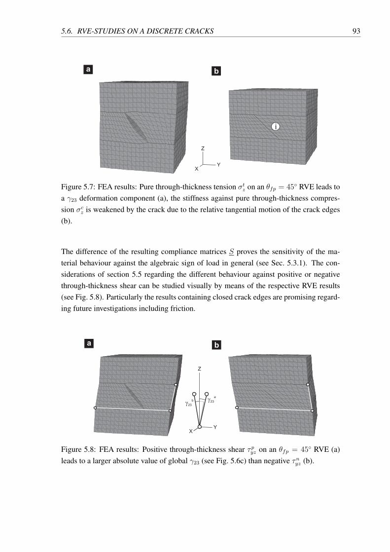
5.6. RVE-STUDIES ON A DISCRETE CRACKS 93
XY
Z
a b
i
Figure 5.7: FEA results: Pure through-thickness tension 𝜎𝑡𝑧 on an 𝜃𝑓𝑝 = 45∘ RVE leads toa 𝛾23 deformation component (a), the stiffness against pure through-thickness compres-sion 𝜎𝑐𝑧 is weakened by the crack due to the relative tangential motion of the crack edges(b).
The difference of the resulting compliance matrices 𝑆 proves the sensitivity of the ma-terial behaviour against the algebraic sign of load in general (see Sec. 5.3.1). The con-siderations of section 5.5 regarding the different behaviour against positive or negativethrough-thickness shear can be studied visually by means of the respective RVE results(see Fig. 5.8). Particularly the results containing closed crack edges are promising regard-ing future investigations including friction.
XY
Z
a b
g23
a
g23
b
Figure 5.8: FEA results: Positive through-thickness shear 𝜏 𝑝𝑦𝑧 on an 𝜃𝑓𝑝 = 45∘ RVE (a)leads to a larger absolute value of global 𝛾23 (see Fig. 5.6c) than negative 𝜏𝑛𝑦𝑧 (b).
94 CHAPTER 5. POST-FAILURE DEGRADATION ANALYSIS
Results concerning the orthotropic material model
Neglecting the coupling positions of the resulting compliance matrices 𝑆 which have tobe 0 in an orthotropic compliance matrix (see Sec. 3.1.1) and averaging the unbalancedpositions, the results of the discrete crack RVE are transferable to the impact of degrada-tion on the common material parameters of an orthotropic material model 𝐸2, 𝐸3, 𝐺12,𝐺13 and 𝐺23 (see Sec. 5.5). By means of these parameters related to the fracture planeorientation (see Fig. 5.9) the analytical thoughts summarised in section 5.5 are reviewedin the following.
0
1000
2000
3000
4000
5000
6000
7000
8000
9000
0 10 20 30 40 50 60
stiffn
ess [
N/m
m2]
qfp [°]
E2E3G12G13G23 a
c
b
d
0
1000
2000
3000
4000
5000
6000
7000
8000
9000
0 10 20 30 40 50 60
stiffn
ess [
N/m
m2]
qfp [°]
0
1000
2000
3000
4000
5000
6000
7000
8000
9000
0 10 20 30 40 50 60
stiffn
ess [
N/m
m2]
qfp [°]
0
1000
2000
3000
4000
5000
6000
7000
8000
9000
0 10 20 30 40 50 60
stiffn
ess [
N/m
m2]
qfp [°]
ii
iviii
i
ii
i
ii
ii
ii
iiiiv
v
iiiiii
v
v
v
tension & positive shear tension & negative shear
compression & positive shear compression & negative shear
Figure 5.9: Orthotropic stiffnesses derived from the compliance matrices of different vir-tual material test sets: (a) tensile loads and positive shear loads, (b) tensile loads andnegative shear loads, (c) compressive loads and positive shear loads and (d) compressiveloads and negative shear loads.
Looking at the reduced stiffnesses resulting from the four load sets (see Fig. 5.9a-d), theorientation-dependent behaviour of 𝐺12 and 𝐺13 is equal in all the four cases (i). Hencetheir insensitivity against the algebraic sign of the shear load assumed in section 5.5 isconfirmed by the RVE results. 𝐺23 behaves equally in both combinations comprisingpositive shear (a and c) and in both combinations comprising negative shear (b and d)hence it does behave sensitive against the algebraic sign of through-thickness shear load
5.6. RVE-STUDIES ON A DISCRETE CRACKS 95
(see Fig. 5.9, ii). The same is the case for 𝐸2 and 𝐸3 which behave in the tensile (aand b) load sets different from the compressive (c and d) ones (see Fig. 5.9, iii). Theresults furthermore confirm that 0∘ IFFs have a large impact on𝐸𝑡
2 whereas𝐸𝑡3 is basically
unaffected (iv). Accordingly these IFFs have the expected impact on 𝐺12 whereas 𝐺13 isunaffected (v).
Figure 5.10 compares the orientation-dependent slope of the RVE results with the stiff-nesses resulting from equation 5.9. The degradation measure 𝜂 has been adjusted to the𝐸𝑡
2 (0∘) so that the crack density of the RVE 𝛿 = 1/3 corresponds to a degradation
progress measure of 𝜂 = 0.678. The shear impact degradation measure 𝑘 has subse-quently been adjusted to meet the 𝐺12 (0
∘) resulting in 𝑘 = 0, 755. This value is close to0.77 proposed for CFRC in section 5.3.1.
a b0
1000
2000
3000
4000
5000
6000
7000
8000
9000
0 10 20 30 40 50 60
Yo
un
g’s
mo
du
li [N
/mm
2]
qfp [°]
0
1000
2000
3000
4000
5000
6000
0 10 20 30 40 50 60
sh
ea
r m
od
uli
[N/m
m2]
qfp [°]
G12
G13
G23+
G23-
E2t
E2c
E3t
E3c
ii
iv
iii
i
v
iv
Figure 5.10: Comparison between the orthotropically reduced results of the RVE and theprediction of the 3D degradation procedure (see Sec. 5.5): (a) Young’s Moduli and (b)shear moduli.
The most obvious difference between the degradation rule and the RVE results is theorientation-dependent behaviour of the compressive Young’s moduli (see Fig. 5.10a, i).While 𝐸𝑐
2 and 𝐸𝑐3 are unaffected by 0∘ IFFs, the assumption that the compressive Young’s
moduli 𝐸𝑐2 and 𝐸𝑐
3 are generally unaffected by IFFs can be identified as strongly sim-plifying by means of the RVE results at highter 𝜃 values. The reason is that the closedcrack edges do transmit the compressive 𝜎𝑛 furthermore, but the tangential load com-ponent arising with a growing 𝜃𝑓𝑝 leads to a tangential motion of the crack edges (seeFig. 5.7b, i). This goes along with the reduction of the effective transverse compressivestiffness 𝐸𝑐
2 and the through-thickness compressive stiffness 𝐸𝑐3 . The amount of this tan-
gential motion depends on the pressure on the crack edges and the friction between them.The presented RVE results are based on a frictionless behaviour, accordingly the effectof IFFs in the compressive stiffnesses is strongly overestimated here and as far as no ex-perimental results are available, it is furthermore suggested to keep 𝐸𝑐
2 and 𝐸𝑐3 constant
96 CHAPTER 5. POST-FAILURE DEGRADATION ANALYSIS
during a degradation analysis.
In the case of 𝐸𝑡3 and 𝐺13 the RVE results and the degradation rule prediction correspond
well. The orientation dependence of 𝐸𝑡2 is however strongly overestimated by the predic-
tion in the examined range of 𝜃𝑓𝑝 = [0∘; 54∘] (see Fig. 5.10a, ii). A virtual material testwith an RVE containing a 90∘ crack proves that the slope of 𝐸𝑡
2 (𝜃𝑓𝑝) rises to its undam-aged value there but the complete slope of the curve is currently unknown. In contrast tothrough-thickness loads, inplane loads are not partly transmitted by sound areas (who’ssize depends on the fracture orientation) but the whole load has to be transmitted over thecrack by the neighbouring laminae no matter what the fracture plane orientation is (seeFig. 5.2a). Being 𝜃𝑓𝑝 = 90∘ the only exception from this, such a slope is not sufficientlypredictable by equation 5.8 and further inquiries are necessary. The same is the case forthe slope of the stiffness against the second inplane load 𝐺12 (see Fig. 5.10b, iii). Cur-rently it cannot be decided whether it is more accurate to run a post-failure analysis witha 𝜃𝑓𝑝-independent 𝐸𝑡
2 and 𝐺12 which neglects the exceptional position of 90∘ cracks or touse equation 5.8.
Looking at the shear moduli at 𝜃𝑓𝑝 = 0∘, the common 𝑘 value which is adjusted to𝐺𝑡12 (0
∘)
results in good predictions for 𝐺23 (0∘) and 𝐺13 in general (see Fig. 5.10b, iv). This sug-
gest to keep the proposed ratios between the degradation of Young’s and shear moduli (seeSec. 5.3.1) unchanged for the 3D post failure degradation analysis. Although the slopesof 𝐺23 generally differ between RVE and prediction (v), the different character of 𝐺+
23
and 𝐺−23 is met by equation 5.9 and it can reasonably be used until further experimental
results become available.
Regarding the fibre-parallel 1-direction the RVE results prove that 𝐸1, 𝜈12 and 𝜈13 areunaffected by any IFF orientation but 𝜈23 changes with different 𝜃𝑓𝑝 and even leaves thecommon range [0; 0.5] for homogeneous materials. This is judged to be reasonable dueto the fact that here a continuum-based material model is used to describe the generalbehaviour of an non-continuous structure. Without reasonable analytical thoughts (seeSec. 5.5) however, there is currently no description of 𝜈23 (𝜃𝑓𝑝) suggested.
In summary the comparison between RVE virtual material test results and the 3D degra-dation rule (see Sec. 5.5) document the general applicability of the presented rules. Inthat context it is important to have in mind that the RVE itself contains significant sim-plifications like the lack of friction between the crack edges. Furthermore the influenceof the constitutive behaviour of the two neighbouring laminae is completely unknown atthis time just as the influence of micro-delamination (see Sec. 2.2.3 and Fig. 2.3d, ii).Generally the reduction of the compliance matrices to an orthotropic material model isas arguable as the representation of the constitutive behaviour of a damaging lamina by
5.6. RVE-STUDIES ON A DISCRETE CRACKS 97
such a continuum-based model itself. Accordingly the presented comparison is not rec-ommended as the basis of any parameter fitting.
Studies on residual stiffnesses
After having reached the saturated crack density, a confined lamina is still transmittingload (see Sec. 2.3). This fact is included in the smeared crack representation by resid-ual stiffnesses which are constantly assigned to the damaged lamina after the degradationprocess has reached the saturated level (see Sec. 5.3.2). Numerous experiments suggestthat the assumption of the saturated crack density at 𝛿 = 1 is a reasonable guess for amajority of UD fibre reinforced 0∘/90∘ laminates under inplane tensile load independentfrom their lamina thickness [100–102]. Although newer investigations revealed a signif-icant dependence on load types and laminate stacking sequences [30, 103], the presenteddiscrete crack RVE has geometrically been adjusted to represent a 𝛿 = 1 crack density of0∘ IFFs. Using the materials given in the WWFE-II (see Ch. 7) the results of the virtualmaterial tests with an applied tensile 𝜎𝑡𝑦 provide first information about the significanceof the numerical approach for the determination of residual stiffnesses (see Tab. 5.2).
MaterialIM7 T300 A-S S2-glass E-glass
8851-7 PR-319 Epoxy1 Epoxy2 MY750CFRC GFRC
𝜂𝐸𝑡
2𝑅 0.31 0.31 0.29 0.26 0.22
𝜂𝐺12𝑅 0.67 0.77 0.69 0.83 0.83
Table 5.2: Results of a 0∘ RVE representing the crack density 𝛿 = 1: Residual stiffnessfraction 𝜂𝑅 .
It has been found, that in the present RVE geometry the maximum stresses in the damagedlamina is below the IFF fracture criterion, thus the analysed crack density 𝛿 = 1 representsa state of damage beyond the saturated crack density which will never be reached inreality. Hence the resulting residual stiffness fraction values (see Tab. 5.2) are generallysuspected to be underestimated.
Keeping in mind that neither this RVE analysis includes micro-defects or micro-delamination (see Sec. 2.2.3) nor it is known how close the actual saturated crack densityis to the assumed value 𝛿 = 1, it is less surprising that the values above do not corre-late well with those determined experimentally (see Sec. 5.3.1 and [88]). The results doconfirm the finding, that the residual shear modulus fraction is higher that the residual
98 CHAPTER 5. POST-FAILURE DEGRADATION ANALYSIS
Young’s Modulus fraction. The numerical 𝜂𝐸𝑡2
𝑅 however is ten times larger than the ex-perimental value 0.03 from [88] which itself is the lowest value compared with numerousother sources [100–103]. Looking at CFRC the 𝜂𝐺12
𝑅 values correspond well with the ex-perimentally determined value of 0.6 but the lower experimental value for GFRC is notnumerically confirmed. Using the same RVE geometry only differing by the material’sconstitutive behaviour does not explain the experimentally determined difference betweenCFRC and GFRC residual stiffnesses. As a result these two groups of materials are ei-ther expected to differ due to a different evolution of those damage types which are notincluded in the RVE or due to different saturated crack densities. Furthermore the influ-ence of the constitutive behaviour of the neighbouring laminae is currently unknown anda subject of further investigations.
5.7 Application-oriented summary
The current post-failure degradation implementation developed in this work (see Ch. 6) in-cludes the constant IFF stress exposure approach 𝑓𝐸 𝐼𝐹𝐹 = 1 = 𝑐𝑜𝑛𝑠𝑡𝑎𝑛𝑡 (see Sec. 5.3.2)to govern the degradation progress represented by the degradation progress measure 𝜂.The degradation’s impact on the different orthotropic stiffnesses of the damaging laminadepends on the orientation of the IFF fracture plane and is implemented by the developed3D degradation procedure (see Sec. 5.5). The reduced stiffnesses of the damaging laminaresult from the orientation impact measure 𝑛 applied to the respective original stiffnesses(see Eq. 5.9) whereas 𝑛 (𝜃𝑓𝑝) (see Eq. 5.8 and Tab. 5.1) preliminary follows the results ofbasic considerations (see Figs. 5.3 and 5.4). Their comparison with virtual material tests(see Sec. 5.6) revealed an acceptable level of agreement which qualifies the developed3D degradation routine for a general application for the time being. The residual stiffnessfraction values are currently taken from [88].
The implemented approach reliably results in an orthotropic lamina behaviour not onlyvalid for the load which led to the respective state of damage but for an arbitrary load casewith arbitrary combinations of positive and negative stress components. The approachgives reasonable results for both stable and unstable degradation processes (see Sec. 5.1)and identifies fibre-perpendicular compressive load cases leading to the hazardous wedgeeffect or an unpredictable crushing by a degradation locking (see Sec. 5.3.2).
6 Implementation of Puck’s Theory in ABAQUS
The implementation of Puck’s fracture criteria and post-failure degradation rules com-pletes the prediction capabilities of commercial FE packages regarding UD FRCs. Theavailable codes provide a large variety of element definitions for the representation oflaminates and laminate structures (see Sec. 3.3). The inter-laminar behaviour between therespective laminae (delamination, see Sec. 2.2.4) is satisfactory representable by the pro-vided interface elements which predict the separation onset and evolution. With the imple-mentation of Puck’s Theory and its enhancements an FE analysis covers all macroscopicand mesoscopic aspects of damage and damage evolution in UD FRCs (see Sec. 2.1).Puck’s Theory meets FEA on the level of the material description. Whereas the pure fail-ure analysis (see Ch. 4) may be accomplished in form of a post-processing of the stressresults, the presented failure and post-failure analysis (see Ch. 5) requires the presentedimplementation within a subroutine for user-defined material behaviour UMAT [8].
6.1 Implicit and explicit FEA
The difference between an implicit or explicit FEA does not play a central role regard-ing the FE-representation of laminates and laminate structures (see Sec. 3.3) whereas itcomes into play when a user-defined material is to be implemented. Puck’s Theory hasbeen developed and verified for nonrecurring, uninterrupted, slow loading processes withapplied combinations of proportionally increasing stress or strain components [4]. Ac-cordingly Puck’s Theory predicts material behaviour in the quasi-static domain wheretime and thus velocity or inertia do neither play a role nor are considered in the respec-tive material models and the related analyses (in contrast to the dynamic domain). In thecontext of nonlinear FEA the mentioned situation is generally related to an implicit solu-tion of the equation systems. Accordingly the following section describes the generationof a material user subroutine in the case of an implicit FEA in detail. However Puck’sTheory is expected to be transferable to dynamic situations in which generally an explicitsolution approach is recommended. The difference between the implicit and explicit so-lution strategy for differential equations is fundamental not only in terms of mathematicalapproaches [104] but the appropriate choice is up to the user and significantly influencesthe accuracy and the computational costs of an FEA. Note that explicit and implicit ap-proaches are not exclusively attributed to dynamic or quasi-static situations respectively.
100 CHAPTER 6. IMPLEMENTATION OF PUCK’S THEORY IN ABAQUS
Thus the integration steps are commonly referred to as time increments whereas its mean-ing is tacitly reduced to load increments in the case of quasi-static analyses.
Both processes involve a numerical time integration scheme to solve for the unknowndisplacement solution at the end of the respective time step. This solution is the basisfor the calculation of the resulting strains and stresses. Explicit integration schemes (e.g.the Central Difference method [105]) assume a linear change in displacement over eachtime step. They calculate the displacements at the end of the time step based on the statevariables – which include the material description in the case of damage analysis – at thebeginning of the time step. The updated state variables are then the basis for the calcu-lation of the subsequent time step. The procedure corresponds to a linear extrapolationbased on the material’s tangent moduli (see Fig. 3.1) and – in dynamic situations – thevelocity and acceleration at the beginning of the time step.
Implicit integration schemes (e.g. the Newmark Forward Differencing method [106]) as-sume a constant average load increase and – in dynamic situations – constant accelerationover each time step. The governing equation is evaluated at the end of the time stepbased on the actual state variables. The major difference between implicit and explicitalgorithms is that the implicit solution method requires a matrix inversion of the struc-tural stiffness matrix, the explicit solution does not. However, unlike the implicit solutionscheme, which is unconditionally stable for large time steps, the explicit scheme is onlystable if the size of the time step is smaller than the critical time step size for the struc-ture being simulated. The undamped critical time step size is 2/𝜔𝑚𝑎𝑥 (where 𝜔𝑚𝑎𝑥 is thelargest natural circular frequency), which is usually a very small value. This very smalltime step size requirement for stability thereby makes explicit solutions recommendablefor short transient situations. But, even though the number of time steps in an explicitsolution may be orders of magnitude greater than that of an implicit solution, it may bemore efficient than an implicit solution since no matrix inversion is required. Neither animplicit nor explicit solution is the clear winner in all cases.
Regarding the implementation of a degrading material behaviour the difference betweenthe explicit and implicit approach lies in the requirements for the material user subrou-tine. Whereas the explicit approach eventually relies on the definition of the material’sconstitutive behaviour in terms of tangent moduli, there is no corresponding requirementin the case of an the implicit approach. ABAQUS finds an acceptable implicit solutionby guessing a displacement field for the end of the respective time step (called attemptwithin ABAQUS). Based on the actual constitutive behaviour associated with that guessthe solver evaluates whether the equilibrium equations are fulfilled within specified toler-ances or not. If this is not the case the guess will be corrected. Both, the original guess
6.2. USER-DEFINED MATERIAL BEHAVIOUR SUBROUTINE 101
and the corrections are based on the material’s Jacobian Matrix calculated at the end ofthe past time increment or attempt. This matrix defines the change of the resulting stresscomponent increments depending on a change of each individual strain component in-crements ∂△ 𝜎/∂△ 𝜖. It effectively includes information corresponding to the tangentstiffnesses which means that in both cases their definition is inevitable. In the case of anexplicit approach the quality of the tangent stiffnesses definition directly determines theaccuracy of the results whereas in the implicit case it only influences the quality of theguesses, i.e. it influences the process of solution convergence but not the solution itself.
6.2 User-defined material behaviour subroutine
The presented User-defined material behaviour subroutine (UMAT) is written for implicitFEAs (see Sec. 6.1) and includes all the presented parts of Puck’s Theory for the fibrefracture and inter-fibre fracture prediction (see Ch. 4), of the 3D degradation rule (seeCh. 5) and the nonlinear material behaviour (see Ch. 3) unless otherwise stated in therespective sections.
The task of the UMAT is to provide
∘ the particular state of stress for an input state of strain.
∘ the relevant parameters and state variables of Puck’s failure theory.
∘ the Jacobian matrix ∂△𝜎/∂△𝜖 for all stress/strain components.
The subroutine is provided with the strain at the beginning of the load increment𝜖 𝑏𝑒𝑔𝑖𝑛 𝑖𝑛𝑐𝑟., the guessed strain increment for the current load increment Δ𝜖 𝑖𝑛𝑐𝑟. and thedegradation progress 𝜂 𝑏𝑒𝑔𝑖𝑛 𝑖𝑛𝑐𝑟. by the main program and follows a straight forwardstructure to determine the associated stresses and failure or degradation parameters (seeFig. 6.1). If the respective load increment is part of the failure analysis period 𝜂 = 1
(see Fig. 2.5), the stiffnesses are derived from given nonlinear stress strain relations (seeSec. 3.1.2). If the respective increment is part of the post-failure period 𝜂 < 1, the reducedstiffnesses are derived from the stiffness reduction process according to equation 5.9. Theresulting stresses are calculated based on the orthotropic material law (see Eq. 3.3). Fromthese stresses, the fibre fracture stress exposure 𝑓𝐸 𝐹𝐹 is derived (see Eq. 4.48) and a FF-flag is switched on if appropriate. Then the IFF stress exposure 𝑓𝐸 𝐼𝐹𝐹 (see Eq. 4.24)is addressed by the calculation of numerous 𝑓𝐸 𝐼𝐹𝐹 (𝜃), currently for 180 different val-ues of 𝜃 (see Eqs. 4.21 and 4.22). The calculated 𝑓𝐸 𝐹𝐹 is then used to determine the
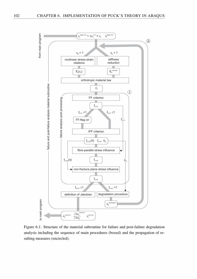
102 CHAPTER 6. IMPLEMENTATION OF PUCK’S THEORY IN ABAQUS
Figure 6.1: Structure of the material subroutine for failure and post-failure degradationanalysis including the sequence of main procedures (boxed) and the propagation of re-sulting measures (encircled).
6.2. USER-DEFINED MATERIAL BEHAVIOUR SUBROUTINE 103
weakening effect 𝜂𝑤1 due to the fibre-parallel stress (see Sec. 4.3.1). The calculated stressexposures of all action planes 𝑓𝐸 𝐼𝐹𝐹 (𝜃) are used to determine the weakening effect 𝜂𝑚+𝑝
due to non-fracture plane stresses (see Sec. 4.3.2). The result is in both cases an increased𝑓𝐸 𝐼𝐹𝐹 . If its value is ≤ 1 at the end, the task of the subroutine is completed and the Jako-bian matrix is determined by a difference quotient approach. In the case of 𝑓𝐸 𝐼𝐹𝐹 > 0
the degradation progress measure 𝜂 is decreased by a predefined increment or ratio andthe orientation impact degradation measures 𝑛𝑖𝑗 are calculated from 𝜃𝑓𝑝 (see Eq. 5.8). Theoverall impact of the degradation on the respective stiffnesses is represented by stiffness-specific 𝜂𝑖𝑗 values and the degradation loop is started. The degradation measure 𝜂 whichfulfils the 𝑓𝐸 𝐼𝐹𝐹 = 1 requirement is determined iteratively.
Figure 6.1 reveals that the failure analysis part of the subroutine (i) may be separated toact as a pure post-processing for conventionally derived FEA stress results or even forexisting stress fields. Hence the application of Puck’s failure criteria requires a relativelysmall adaption of common analysis procedures without the need for further theoreticalstudies of FE solution approaches, material definition requirements and the associatedsyntax of the respective software. The computational cost for the determination of thestress exposure values is definitely small compared to the knowledge gain regarding theanalysed laminate or laminate structure. On the other hand, the implementation of Puck’sTheory including degradation (see Fig. 6.1, ii) is a procedure which resides deeper insidethe FEA. Numerical matters like load increment size, determination algorithm for theJacobian, the degradation progress increments and numerical damping parameters haveto be adjusted carefully to ensure accurate results and acceptable computational effort[107].
The presented subroutine contains two iterative parameter-determinations which is gener-ally inefficient and complicates the application of Puck’s Theory within an explicit FEAcontext. There the small time increments require the material subroutine to run extremelyoften and iterative procedures are serious disadvantages. Accordingly there are currentattempts to express the 𝑓𝐸 𝐼𝐹𝐹 (𝜃𝑓𝑝) in a closed analytical form as already possible inthe case of inplane load [4]. The same is aimed for the determination of the degrada-tion progress measure 𝜂 and – in the ultimate consequence – also for the Jacobian matrix[108].

7 World Wide Failure Exercise II
After the World Wide Failure Exercise which addressed inplane failure and post failureprediction of UD FRPCs [2], a second World-Wide Failure Exercise (WWFE-II) waslaunched by Kaddour and Hinton [69], to assess the capability and maturity of current3D failure criteria. In the exercise, the originators of composite failure theories were in-vited to take part by agreeing to provide two papers (Part A and Part B) describing theirmodel and its correlation with test data. The organisers provided a set of 12 test cases(see App. B.3) to challenge the current failure criteria, a set of material parameters (seeApp. B.2) and a set of guidelines (see App. B.1). The author, after a personal consultationwith Puck, has accepted to participate as the exercise was seen to provide an opportunityto illustrate the usefulness of Puck’s Theory and to validate its applicability to problemsinvolving 3D stresses [109]. The results presented below (see Sec. 7.2) are blind pre-dictions based on the provided information. The generation of these results involves thepreparation of Puck’s failure (see Ch. 4) and post failure approaches for an unrestrictedthree-dimensional use (see Ch. 5), the implementation into a powerfull FE stress analysisenvironment (see Ch. 6) and the identification and solution of particular problems arisingfrom the individual load cases. This includes the considerations about 3D degradationpresented below before the actual test case results are discussed in section 7.2.
7.1 Degradation aspects of the WWFE-II
In order to ensure the unlimited 3D applicability of the developed approaches and analysistools, the whole work aims on general three-dimensional load cases, particular in terms ofpost-failure degradation (see Ch. 5). However load redistribution from weaker to strongerlaminae is excluded in cases where any load has to be transmitted in through-thicknessdirection of the laminate (𝜎𝑧, 𝜏𝑥𝑧 and 𝜏𝑦𝑧 namely) or where all the laminae are experienc-ing equal stress exposures. In these cases a lamina can not dispose of any load reducingits stiffness. From the numerical point of view the smallest further increase of the appliedload leads to an immediate increase of the crack density up to infinity. This process iscalled unstable degradation (see Sec. 5.1). Neglecting damping or statistical effects, intheses cases the curves of initial and final failure stress coincide.
After reaching the final failure stress there are laminate and load configurations which
106 CHAPTER 7. WORLD WIDE FAILURE EXERCISE II
allow a further deformation of the material at constant or declining applied loads beforeit completely disintegrates. As Puck’s Theory is stress based on the one hand and thedefinition of a complete disintegration is arguable on the other hand, there is no finalfailure strain information provided in these cases.
A special case occurs for damage due to compressive 𝜎2 and/or 𝜎3 in a lamina becausethe resulting cracks are still capable of transmitting compressive forces in the respectivedirections. In these cases the lamina does transmit increasing applied stresses after ex-ceeding the IFF fracture criterion up to a point where the laminate starts breaking due tothe wedge effect or starts crushing due to through-thickness compression (see Sec. 5.3.2).Both effects are ruled by mechanisms on a microscopic level far below the capabilitiesof a smeared crack representation and a continuum-based constitutive model. The ongo-ing effort of covering such damage evolutions by granular media-based simulations [110]has not reached a level of applicability to classify the processes as a predictable – hencetolerable – damage evolution. As long as this is not the case the limits of applicationare considered to be reached when the stress exposure in one or more laminae reaches𝑓𝐸 = 1.
Regarding the WWFE-II none of the test cases meets the above mentioned requirementsfor a reliably stable post-failure degradation. Where the test cases ask for failure stresses(see test cases 8, 10 and 11, Secs. 7.2.3 and 7.2.3) the initial and final failure curve fol-lowing the above definition coincide. Only a few load cases of test case 8 are consideredto reach a final fibre failure after an initial inter-fibre failure. In test case 9 (see Sec. 7.2.3)all laminae are experiencing an equal stress exposure and in test case 12 (see Sec. 7.2.3)the applied pressure 𝜎𝑧 leads to damage resulting from compressive 𝜎3 in the lamina.
7.2 Results of the WWFE-II test cases
The developed user-defined material subroutine (see Ch. 6) is employed to predict the re-sponse of 12 test cases provided by the organisers of the WWFE-II. These test cases coverpure, isotropic polymer material (see Sec. 7.2.1), unidirectional laminae (see Sec. 7.2.2)and multidirectional laminates (see Sec. 7.2.3) made from glass/epoxy and carbon/epoxy.The cases include full three-dimensional loadings including superposed shear. The detailsof material properties, lay-ups and loadings as well as guidelines are described in [69] andappendix B. The following presentation of the results is not only intended to prove theapplicability and versatility of Puck’s Theory and its implementation but it provides use-ful examples for the understanding of the complex lamina and laminate behaviour andthe functionality of Puck’s Theory in particular. For this purpose every test case setup is
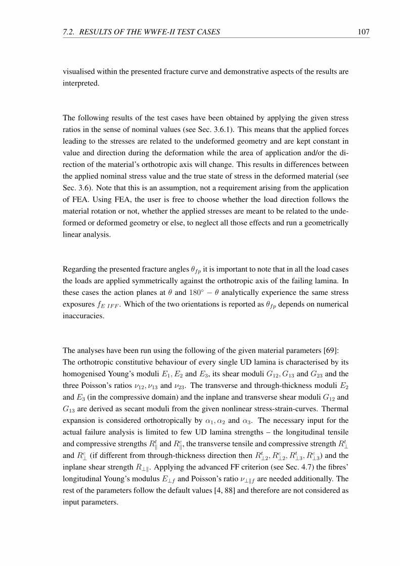
7.2. RESULTS OF THE WWFE-II TEST CASES 107
visualised within the presented fracture curve and demonstrative aspects of the results areinterpreted.
The following results of the test cases have been obtained by applying the given stressratios in the sense of nominal values (see Sec. 3.6.1). This means that the applied forcesleading to the stresses are related to the undeformed geometry and are kept constant invalue and direction during the deformation while the area of application and/or the di-rection of the material’s orthotropic axis will change. This results in differences betweenthe applied nominal stress value and the true state of stress in the deformed material (seeSec. 3.6). Note that this is an assumption, not a requirement arising from the applicationof FEA. Using FEA, the user is free to choose whether the load direction follows thematerial rotation or not, whether the applied stresses are meant to be related to the unde-formed or deformed geometry or else, to neglect all those effects and run a geometricallylinear analysis.
Regarding the presented fracture angles 𝜃𝑓𝑝 it is important to note that in all the load casesthe loads are applied symmetrically against the orthotropic axis of the failing lamina. Inthese cases the action planes at 𝜃 and 180∘ − 𝜃 analytically experience the same stressexposures 𝑓𝐸 𝐼𝐹𝐹 . Which of the two orientations is reported as 𝜃𝑓𝑝 depends on numericalinaccuracies.
The analyses have been run using the following of the given material parameters [69]:The orthotropic constitutive behaviour of every single UD lamina is characterised by itshomogenised Young’s moduli 𝐸1, 𝐸2 and 𝐸3, its shear moduli 𝐺12, 𝐺13 and 𝐺23 and thethree Poisson’s ratios 𝜈12, 𝜈13 and 𝜈23. The transverse and through-thickness moduli 𝐸2
and 𝐸3 (in the compressive domain) and the inplane and transverse shear moduli 𝐺12 and𝐺13 are derived as secant moduli from the given nonlinear stress-strain-curves. Thermalexpansion is considered orthotropically by 𝛼1, 𝛼2 and 𝛼3. The necessary input for theactual failure analysis is limited to few UD lamina strengths – the longitudinal tensileand compressive strengths 𝑅𝑡
∥ and 𝑅𝑐∥, the transverse tensile and compressive strength 𝑅𝑡
⊥and 𝑅𝑐
⊥ (if different from through-thickness direction then 𝑅𝑡⊥2, 𝑅
𝑐⊥2, 𝑅
𝑡⊥3, 𝑅
𝑐⊥3) and the
inplane shear strength 𝑅⊥∥. Applying the advanced FF criterion (see Sec. 4.7) the fibres’longitudinal Young’s modulus 𝐸⊥𝑓 and Poisson’s ratio 𝜈⊥∥𝑓 are needed additionally. Therest of the parameters follow the default values [4, 88] and therefore are not considered asinput parameters.
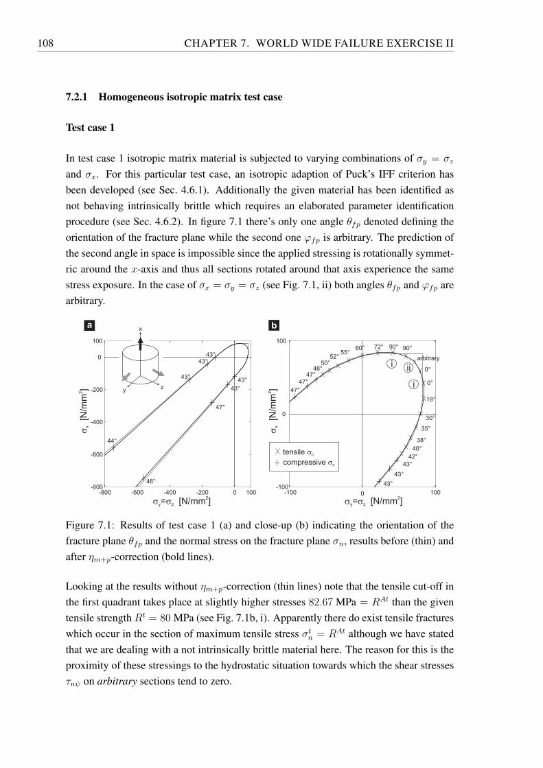
108 CHAPTER 7. WORLD WIDE FAILURE EXERCISE II
7.2.1 Homogeneous isotropic matrix test case
Test case 1
In test case 1 isotropic matrix material is subjected to varying combinations of 𝜎𝑦 = 𝜎𝑧
and 𝜎𝑥. For this particular test case, an isotropic adaption of Puck’s IFF criterion hasbeen developed (see Sec. 4.6.1). Additionally the given material has been identified asnot behaving intrinsically brittle which requires an elaborated parameter identificationprocedure (see Sec. 4.6.2). In figure 7.1 there’s only one angle 𝜃𝑓𝑝 denoted defining theorientation of the fracture plane while the second one 𝜑𝑓𝑝 is arbitrary. The prediction ofthe second angle in space is impossible since the applied stressing is rotationally symmet-ric around the 𝑥-axis and thus all sections rotated around that axis experience the samestress exposure. In the case of 𝜎𝑥 = 𝜎𝑦 = 𝜎𝑧 (see Fig. 7.1, ii) both angles 𝜃𝑓𝑝 and 𝜑𝑓𝑝 arearbitrary.
-800
-600
-400
-200
0
-800 -600 -400 -200 0
sx
[N/m
m]
2
sy z=s [N/mm ]2
100
100 1000-100
0
100
-100
sx
[N/m
m]
2
sy z= [N/mm ]2
s
a b
43°
43°43°
47°
47°
47°
50°52°
55°60° 72° 90° 90°
arbitrary
0°
0°
18°
30°
35°
38°
40°
43°
43°
43°
43°
43°
47°
42°
i
i
tensile sn
compressive sn
48°
44°
46°
ii
z
x
y
Figure 7.1: Results of test case 1 (a) and close-up (b) indicating the orientation of thefracture plane 𝜃𝑓𝑝 and the normal stress on the fracture plane 𝜎𝑛, results before (thin) andafter 𝜂𝑚+𝑝-correction (bold lines).
Looking at the results without 𝜂𝑚+𝑝-correction (thin lines) note that the tensile cut-off inthe first quadrant takes place at slightly higher stresses 82.67 MPa = 𝑅𝐴𝑡 than the giventensile strength𝑅𝑡 = 80 MPa (see Fig. 7.1b, i). Apparently there do exist tensile fractureswhich occur in the section of maximum tensile stress 𝜎𝑡𝑛 = 𝑅𝐴𝑡 although we have statedthat we are dealing with a not intrinsically brittle material here. The reason for this is theproximity of these stressings to the hydrostatic situation towards which the shear stresses𝜏𝑛𝜓 on arbitrary sections tend to zero.
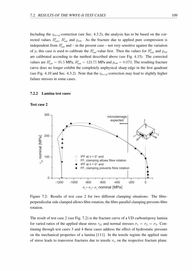
7.2. RESULTS OF THE WWFE-II TEST CASES 109
Including the 𝜂𝑚+𝑝-correction (see Sec. 4.3.2), the analysis has to be based on the cor-rected values 𝑅𝑡
cor, 𝑅𝑐cor and 𝑝cor. As the fracture due to applied pure compression is
independent from 𝑅𝑡cor and – in the present case – not very sensitive against the variation
of 𝑝, this case is used to calibrate the 𝑅𝑐cor-value first. Then the values for 𝑅𝑡
cor and 𝑝cor
are calibrated according to the method described above (see Fig. 4.15). The correctedvalues are 𝑅𝑡
cor = 95.5 MPa, 𝑅𝑐cor = 123.71 MPa and 𝑝cor = 0.073. The resulting fracture
curve does no longer exhibit the completely unphysical sharp edge in the first quadrant(see Fig. 4.10 and Sec. 4.3.2). Note that the 𝜂𝑚+𝑝-correction may lead to slightly higherfailure stresses in some cases.
7.2.2 Lamina test cases
Test case 2
microdamageexpected
[ ]
[
] 1
3
2
Figure 7.2: Results of test case 2 for two different clamping situations: The fibre-perpendicular side clamped allows fibre rotation, the fibre-parallel clamping prevents fibrerotation.
The result of test case 2 (see Fig. 7.2) is the fracture curve of a UD carbon/epoxy laminafor varied ratios of the applied shear stress 𝜏21 and normal stresses 𝜎1 = 𝜎2 = 𝜎3. Con-tinuing through test cases 3 and 4 these cases address the effect of hydrostatic pressureon the mechanical properties of a lamina [111]. In the tensile regime the applied stateof stress leads to transverse fractures due to tensile 𝜎𝑛 on the respective fracture plane.
110 CHAPTER 7. WORLD WIDE FAILURE EXERCISE II
These fractures are promoted by additional 𝜏𝑛1 due to the applied 𝜏21. In the compressiveregime the equal amount of 𝜎2 and 𝜎3 excludes fractures due to 𝜏𝑛𝑡 on any action plane(see Eq. 4.3). At the same time the bearable 𝜏𝑛1 rises with increasing compressive stress𝜎𝑐𝑛 on the fracture plane resulting in a high amount of bearable 𝜏21 if it is combined withhigh 𝜎2 = 𝜎3-values. For a decreasing ratio between 𝜏21 and compressive 𝜎1 = 𝜎2 = 𝜎3
the failure mode eventually changes to fibre fracture due to compressive 𝜎1. Using theextended FF criterion (see Sec. 4.7), the lamina bears more compressive 𝜎1 than the givenlongitudinal compressive strength 𝑅𝑐
∥ = 950 MPa. The according true FF stress is −1463
MPa, which is reached at the plotted nominal value of −1165 MPa.
Although having stated that a compressive 𝜎2 = 𝜎3 does not lead to an IFF according tothe application of Puck’s Theory, which predicts – by definition – macroscopic fracture,there are experimental findings that micro-damage starts at 𝜎2 = 𝜎3 ≈ −2𝑅𝑐
⊥. Thisconclusion has been drawn from acoustic emission studies [23], but the prediction ofthese micro-defects merging to a macroscopic crack [110] is still a challenging task andfar beyond engineering application. Hence the corresponding thresholds are included (seeSecs. 7.2.2 and 7.2.2) for information only but there is the possibility that micro-defectsmerge to macroscopic IFF before the predicted failures at high hydrostatic pressures mayoccur.
The high amount of bearable 𝜏21 leads to a considerable change in fibre direction if per-mitted by the applied boundary conditions. For the nominal hydrostatic pressure of −600
MPa the 𝛾21-results of test case 4 (see Fig. 7.4) provide the magnitude of the fibres’ ro-tation. Rotations of that magnitude increase the discrepancy between applied nominalstresses and the true stresses which the failure analysis is based on. Therefore the plotshows the results for two different boundary conditions where either the (𝑥1, 𝑥3)- or the(𝑥2, 𝑥3)-plane of the material is fixed in space. Regarding the FF, the bearable 𝜎1 slightlyincreases with rotated fibres because now 𝜎1 is only partly acting in the fibre’s longitudinaldirection.
Note that in the present case of a geometrically nonlinear analysis the constitutive be-haviour influences the stress results as they are derived from the deformed geometry (seeSec. 3.6). As the bearable shear stresses are considerably above those bearable under apure 𝜏21-loading, the given nonlinear 𝜏21(𝛾21)-relation is exceeded. In such cases we haveproposed the use of a self-similarly scaled stress-strain relation (see Sec. 3.1.2). Howeverin the present case of rather small nonlinearities in the given 𝜏21(𝛾21)-relation the effort ofa separate iteration for every point on the fracture curve seems not rewarding, hence wedecided to step back to a linear 𝜏21(𝛾21)-relation for test case 2 and 3.
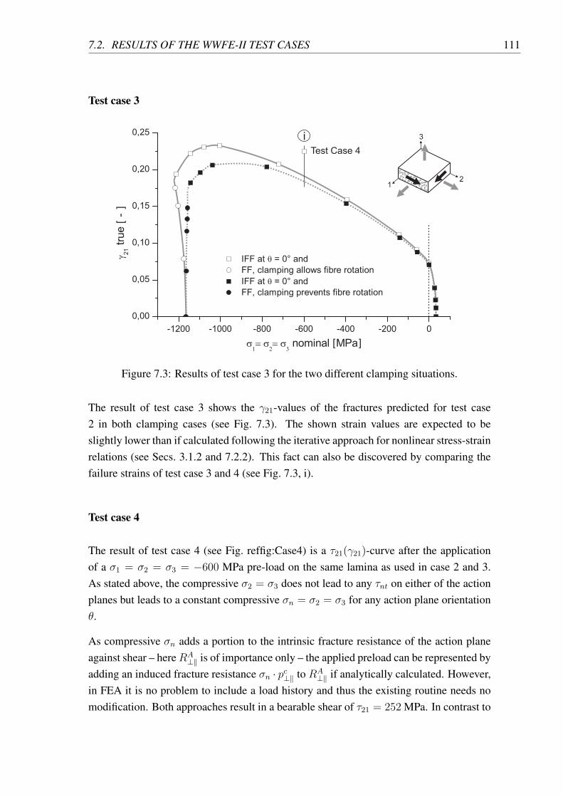
7.2. RESULTS OF THE WWFE-II TEST CASES 111
Test case 3
[ ]
[ ]
i
Test Case 4
1
3
2
Figure 7.3: Results of test case 3 for the two different clamping situations.
The result of test case 3 shows the 𝛾21-values of the fractures predicted for test case2 in both clamping cases (see Fig. 7.3). The shown strain values are expected to beslightly lower than if calculated following the iterative approach for nonlinear stress-strainrelations (see Secs. 3.1.2 and 7.2.2). This fact can also be discovered by comparing thefailure strains of test case 3 and 4 (see Fig. 7.3, i).
Test case 4
The result of test case 4 (see Fig. reffig:Case4) is a 𝜏21(𝛾21)-curve after the applicationof a 𝜎1 = 𝜎2 = 𝜎3 = −600 MPa pre-load on the same lamina as used in case 2 and 3.As stated above, the compressive 𝜎2 = 𝜎3 does not lead to any 𝜏𝑛𝑡 on either of the actionplanes but leads to a constant compressive 𝜎𝑛 = 𝜎2 = 𝜎3 for any action plane orientation𝜃.
As compressive 𝜎𝑛 adds a portion to the intrinsic fracture resistance of the action planeagainst shear – here𝑅𝐴
⊥∥ is of importance only – the applied preload can be represented byadding an induced fracture resistance 𝜎𝑛 ⋅ 𝑝𝑐⊥∥ to 𝑅𝐴
⊥∥ if analytically calculated. However,in FEA it is no problem to include a load history and thus the existing routine needs nomodification. Both approaches result in a bearable shear of 𝜏21 = 252 MPa. In contrast to
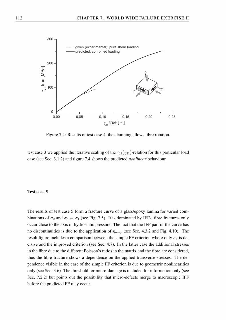
112 CHAPTER 7. WORLD WIDE FAILURE EXERCISE II
[ ]
[ ]
1
3
2
Figure 7.4: Results of test case 4, the clamping allows fibre rotation.
test case 3 we applied the iterative scaling of the 𝜏21(𝛾21)-relation for this particular loadcase (see Sec. 3.1.2) and figure 7.4 shows the predicted nonlinear behaviour.
Test case 5
The results of test case 5 form a fracture curve of a glass/epoxy lamina for varied com-binations of 𝜎2 and 𝜎3 = 𝜎1 (see Fig. 7.5). It is dominated by IFFs, fibre fractures onlyoccur close to the axis of hydrostatic pressure. The fact that the IFF part of the curve hasno discontinuities is due to the application of 𝜂𝑚+𝑝 (see Sec. 4.3.2 and Fig. 4.10). Theresult figure includes a comparison between the simple FF criterion where only 𝜎1 is de-cisive and the improved criterion (see Sec. 4.7). In the latter case the additional stressesin the fibre due to the different Poisson’s ratios in the matrix and the fibre are considered,thus the fibre fracture shows a dependence on the applied transverse stresses. The de-pendence visible in the case of the simple FF criterion is due to geometric nonlinearitiesonly (see Sec. 3.6). The threshold for micro-damage is included for information only (seeSec. 7.2.2) but points out the possibility that micro-defects merge to macroscopic IFFbefore the predicted FF may occur.
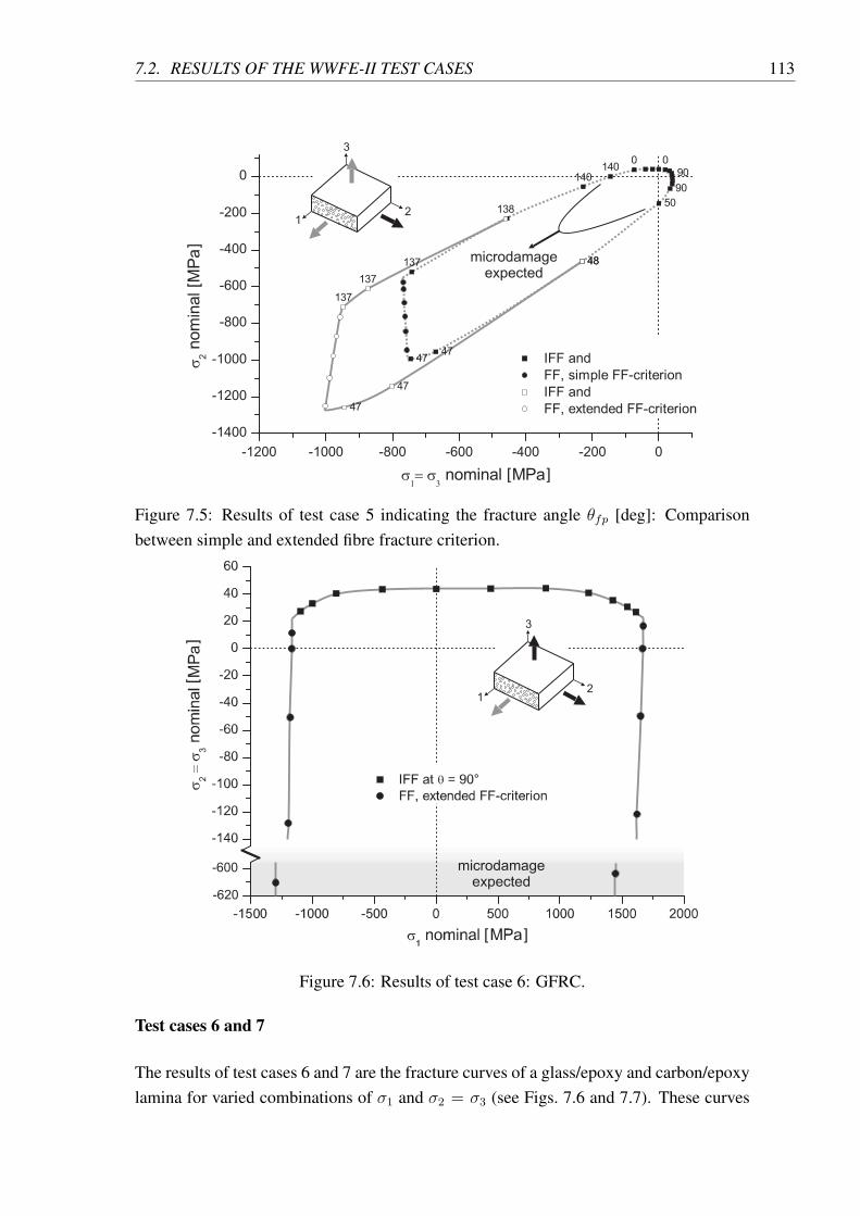
7.2. RESULTS OF THE WWFE-II TEST CASES 113
microdamageexpected
[ ]
[ ]
1
3
2
Figure 7.5: Results of test case 5 indicating the fracture angle 𝜃𝑓𝑝 [deg]: Comparisonbetween simple and extended fibre fracture criterion.
[ ]
[ ]
-600
-620
microdamageexpected
1
3
2
Figure 7.6: Results of test case 6: GFRC.
Test cases 6 and 7
The results of test cases 6 and 7 are the fracture curves of a glass/epoxy and carbon/epoxylamina for varied combinations of 𝜎1 and 𝜎2 = 𝜎3 (see Figs. 7.6 and 7.7). These curves
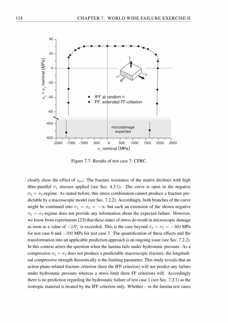
114 CHAPTER 7. WORLD WIDE FAILURE EXERCISE II
microdamageexpected
[ ]
[ ]
-600
-620
1
3
2
Figure 7.7: Results of test case 7: CFRC.
clearly show the effect of 𝜂𝑤1: The fracture resistance of the matrix declines with highfibre-parallel 𝜎1 stresses applied (see Sec. 4.3.1). The curve is open in the negative𝜎2 = 𝜎3-regime. As stated before, this stress combination cannot produce a fracture pre-dictable by a macroscopic model (see Sec. 7.2.2). Accordingly, both branches of the curvemight be continued into 𝜎2 = 𝜎3 = −∞ but such an extension of the shown negative𝜎2 = 𝜎3-regime does not provide any information about the expected failure. However,we know from experiments [23] that these states of stress do result in microscopic damageas soon as a value of −2𝑅𝑐
⊥ is exceeded. This is the case beyond 𝜎2 = 𝜎3 = −360 MPafor test case 6 and −300 MPa for test case 7. The quantification of these effects and thetransformation into an applicable prediction approach is an ongoing issue (see Sec. 7.2.2).In this context arises the question when the lamina fails under hydrostatic pressure. As acompressive 𝜎2 = 𝜎3 does not produce a predictable macroscopic fracture, the longitudi-nal compressive strength theoretically is the limiting parameter. This study reveals that anaction plane-related fracture criterion (here the IFF criterion) will not predict any failureunder hydrostatic pressure whereas a stress limit (here FF criterion) will. Accordinglythere is no prediction regarding the hydrostatic failure of test case 1 (see Sec. 7.2.1) as theisotropic material is treated by the IFF criterion only. Whether – in the lamina test cases
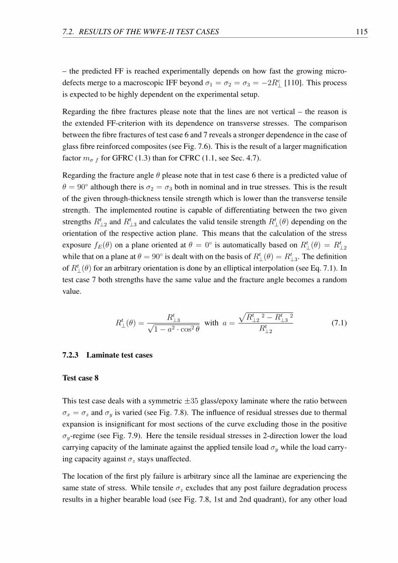
7.2. RESULTS OF THE WWFE-II TEST CASES 115
– the predicted FF is reached experimentally depends on how fast the growing micro-defects merge to a macroscopic IFF beyond 𝜎1 = 𝜎2 = 𝜎3 = −2𝑅𝑐
⊥ [110]. This processis expected to be highly dependent on the experimental setup.
Regarding the fibre fractures please note that the lines are not vertical – the reason isthe extended FF-criterion with its dependence on transverse stresses. The comparisonbetween the fibre fractures of test case 6 and 7 reveals a stronger dependence in the case ofglass fibre reinforced composites (see Fig. 7.6). This is the result of a larger magnificationfactor 𝑚𝜎 𝑓 for GFRC (1.3) than for CFRC (1.1, see Sec. 4.7).
Regarding the fracture angle 𝜃 please note that in test case 6 there is a predicted value of𝜃 = 90∘ although there is 𝜎2 = 𝜎3 both in nominal and in true stresses. This is the resultof the given through-thickness tensile strength which is lower than the transverse tensilestrength. The implemented routine is capable of differentiating between the two givenstrengths 𝑅𝑡
⊥2 and 𝑅𝑡⊥3 and calculates the valid tensile strength 𝑅𝑡
⊥(𝜃) depending on theorientation of the respective action plane. This means that the calculation of the stressexposure 𝑓𝐸(𝜃) on a plane oriented at 𝜃 = 0∘ is automatically based on 𝑅𝑡
⊥(𝜃) = 𝑅𝑡⊥2
while that on a plane at 𝜃 = 90∘ is dealt with on the basis of 𝑅𝑡⊥(𝜃) = 𝑅𝑡
⊥3. The definitionof 𝑅𝑡
⊥(𝜃) for an arbitrary orientation is done by an elliptical interpolation (see Eq. 7.1). Intest case 7 both strengths have the same value and the fracture angle becomes a randomvalue.
𝑅𝑡⊥(𝜃) =
𝑅𝑡⊥3√
1− 𝑎2 ⋅ cos2 𝜃 with 𝑎 =
√𝑅𝑡
⊥22 −𝑅𝑡
⊥32
𝑅𝑡⊥2
(7.1)
7.2.3 Laminate test cases
Test case 8
This test case deals with a symmetric ±35 glass/epoxy laminate where the ratio between𝜎𝑥 = 𝜎𝑧 and 𝜎𝑦 is varied (see Fig. 7.8). The influence of residual stresses due to thermalexpansion is insignificant for most sections of the curve excluding those in the positive𝜎𝑦-regime (see Fig. 7.9). Here the tensile residual stresses in 2-direction lower the loadcarrying capacity of the laminate against the applied tensile load 𝜎𝑦 while the load carry-ing capacity against 𝜎𝑧 stays unaffected.
The location of the first ply failure is arbitrary since all the laminae are experiencing thesame state of stress. While tensile 𝜎𝑧 excludes that any post failure degradation processresults in a higher bearable load (see Fig. 7.8, 1st and 2nd quadrant), for any other load
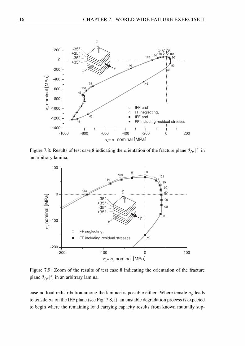
116 CHAPTER 7. WORLD WIDE FAILURE EXERCISE II
x z
y
[ ]
[
]i i i
z
y
x
-35°+35°-35°+35°
Figure 7.8: Results of test case 8 indicating the orientation of the fracture plane 𝜃𝑓𝑝 [∘] inan arbitrary lamina.
x z
y
[ ]
[ ]
z
y
x
-35°+35°-35°+35°
Figure 7.9: Zoom of the results of test case 8 indicating the orientation of the fractureplane 𝜃𝑓𝑝 [∘] in an arbitrary lamina.
case no load redistribution among the laminae is possible either. Where tensile 𝜎𝑦 leadsto tensile 𝜎𝑛 on the IFF plane (see Fig. 7.8, i), an unstable degradation process is expectedto begin where the remaining load carrying capacity results from known mutually sup-
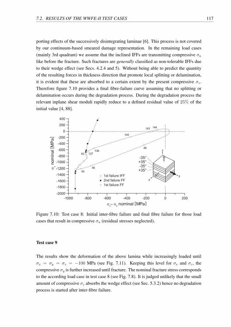
7.2. RESULTS OF THE WWFE-II TEST CASES 117
porting effects of the successively disintegrating laminae [6]. This process is not coveredby our continuum-based smeared damage representation. In the remaining load cases(mainly 3rd quadrant) we assume that the inclined IFFs are transmitting compressive 𝜎𝑛like before the fracture. Such fractures are generally classified as non-tolerable IFFs dueto their wedge effect (see Secs. 4.2.4 and 5). Without being able to predict the quantityof the resulting forces in thickness direction that promote local splitting or delamination,it is evident that these are absorbed to a certain extent by the present compressive 𝜎𝑧.Therefore figure 7.10 provides a final fibre-failure curve assuming that no splitting ordelamination occurs during the degradation process. During the degradation process therelevant inplane shear moduli rapidly reduce to a defined residual value of 25% of theinitial value [4, 88].
y[ ]
-1600
-1800
-2000
400
x z[ ]
1st failure IFF
2nd failure FF
1st failure FF
z
y
x
-35°+35°-35°+35°
Figure 7.10: Test case 8: Initial inter-fibre failure and final fibre failure for those loadcases that result in compressive 𝜎𝑛 (residual stresses neglected).
Test case 9
The results show the deformation of the above lamina while increasingly loaded until𝜎𝑥 = 𝜎𝑦 = 𝜎𝑧 = −100 MPa (see Fig. 7.11). Keeping this level for 𝜎𝑥 and 𝜎𝑧, thecompressive 𝜎𝑦 is further increased until fracture. The nominal fracture stress correspondsto the according load case in test case 8 (see Fig. 7.8). It is judged unlikely that the smallamount of compressive 𝜎𝑧 absorbs the wedge effect (see Sec. 5.3.2) hence no degradationprocess is started after inter-fibre failure.
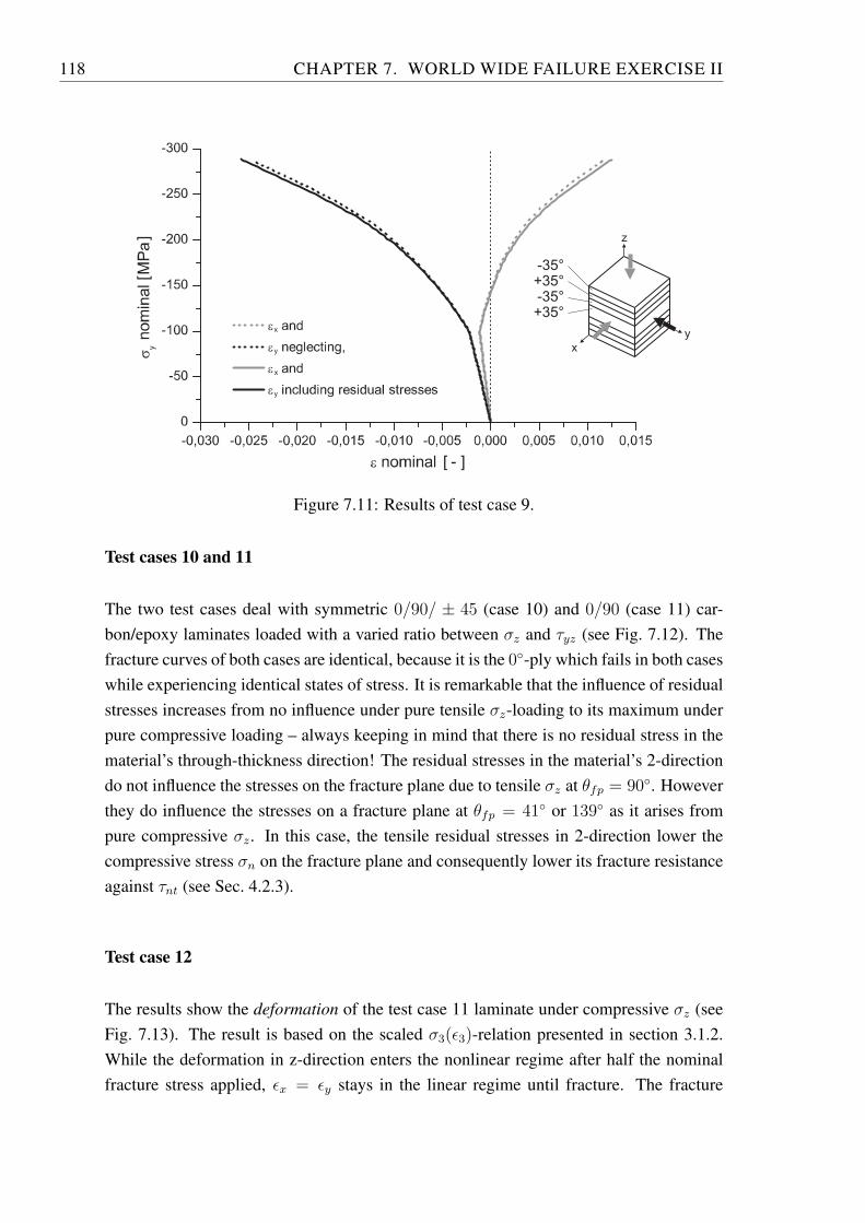
118 CHAPTER 7. WORLD WIDE FAILURE EXERCISE II
x
y
x
yy
[ ]
[
] z
y
x
-35°+35°-35°+35°
Figure 7.11: Results of test case 9.
Test cases 10 and 11
The two test cases deal with symmetric 0/90/ ± 45 (case 10) and 0/90 (case 11) car-bon/epoxy laminates loaded with a varied ratio between 𝜎𝑧 and 𝜏𝑦𝑧 (see Fig. 7.12). Thefracture curves of both cases are identical, because it is the 0∘-ply which fails in both caseswhile experiencing identical states of stress. It is remarkable that the influence of residualstresses increases from no influence under pure tensile 𝜎𝑧-loading to its maximum underpure compressive loading – always keeping in mind that there is no residual stress in thematerial’s through-thickness direction! The residual stresses in the material’s 2-directiondo not influence the stresses on the fracture plane due to tensile 𝜎𝑧 at 𝜃𝑓𝑝 = 90∘. Howeverthey do influence the stresses on a fracture plane at 𝜃𝑓𝑝 = 41∘ or 139∘ as it arises frompure compressive 𝜎𝑧. In this case, the tensile residual stresses in 2-direction lower thecompressive stress 𝜎𝑛 on the fracture plane and consequently lower its fracture resistanceagainst 𝜏𝑛𝑡 (see Sec. 4.2.3).
Test case 12
The results show the deformation of the test case 11 laminate under compressive 𝜎𝑧 (seeFig. 7.13). The result is based on the scaled 𝜎3(𝜖3)-relation presented in section 3.1.2.While the deformation in z-direction enters the nonlinear regime after half the nominalfracture stress applied, 𝜖𝑥 = 𝜖𝑦 stays in the linear regime until fracture. The fracture
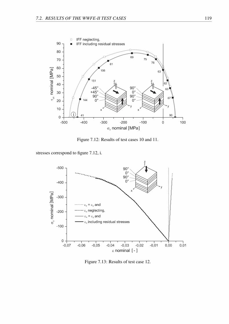
7.2. RESULTS OF THE WWFE-II TEST CASES 119
z
yz
[ ]
[ ]
i
z
y
x
90°0°
90°0°
z
y
x
-45°+45°
90°0°
Figure 7.12: Results of test cases 10 and 11.
stresses correspond to figure 7.12, i.
x
z
y
x
z
y
z
[ ]
[ ]
z
y
x
90°0°
90°0°
Figure 7.13: Results of test case 12.

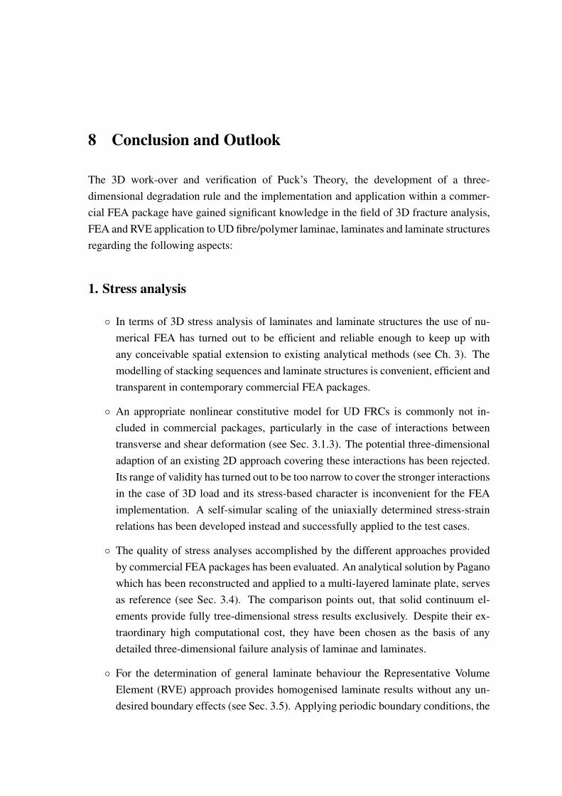
8 Conclusion and Outlook
The 3D work-over and verification of Puck’s Theory, the development of a three-dimensional degradation rule and the implementation and application within a commer-cial FEA package have gained significant knowledge in the field of 3D fracture analysis,FEA and RVE application to UD fibre/polymer laminae, laminates and laminate structuresregarding the following aspects:
1. Stress analysis
∘ In terms of 3D stress analysis of laminates and laminate structures the use of nu-merical FEA has turned out to be efficient and reliable enough to keep up withany conceivable spatial extension to existing analytical methods (see Ch. 3). Themodelling of stacking sequences and laminate structures is convenient, efficient andtransparent in contemporary commercial FEA packages.
∘ An appropriate nonlinear constitutive model for UD FRCs is commonly not in-cluded in commercial packages, particularly in the case of interactions betweentransverse and shear deformation (see Sec. 3.1.3). The potential three-dimensionaladaption of an existing 2D approach covering these interactions has been rejected.Its range of validity has turned out to be too narrow to cover the stronger interactionsin the case of 3D load and its stress-based character is inconvenient for the FEAimplementation. A self-simular scaling of the uniaxially determined stress-strainrelations has been developed instead and successfully applied to the test cases.
∘ The quality of stress analyses accomplished by the different approaches providedby commercial FEA packages has been evaluated. An analytical solution by Paganowhich has been reconstructed and applied to a multi-layered laminate plate, servesas reference (see Sec. 3.4). The comparison points out, that solid continuum el-ements provide fully tree-dimensional stress results exclusively. Despite their ex-traordinary high computational cost, they have been chosen as the basis of anydetailed three-dimensional failure analysis of laminae and laminates.
∘ For the determination of general laminate behaviour the Representative VolumeElement (RVE) approach provides homogenised laminate results without any un-desired boundary effects (see Sec. 3.5). Applying periodic boundary conditions, the
122 CHAPTER 8. CONCLUSION AND OUTLOOK
results represent the material behaviour of the entire laminate independent from itslateral extensions.
∘ The ability of contemporary FEA packages to perform geometrically nonlinearanalysis is particularly valuable in the present case. When running a geometricallynonlinear FE analysis the incremental load is applied to the deformed geometry.Regarding UD composites this means that fibre rotations are considered in all theresults automatically (see Secs. 3.6 and 7.2.2).
∘ Regarding thermal residual stresses, the combination of Puck’s Theory and FEAoffers a complete decoupling of the failure analysis from that topic. The coolingdown process of the laminate is represented in a separate analysis step before theouter load is applied. The following failure analysis needs no modification, whetherthermal stresses are considered or not (see Sec. 3.7).
2. Puck’s failure theory
∘ The physical and fracture mechanical basis and the spacial character of Puck’s fibre-and inter-fibre fracture criteria have been thoroughly approved by the present work.Where adaptions of the previously published relations have been made they are tobe attributed to the commonly inplane focussing of the model’s application, neverto two-dimensional restrictions of the actual theory (see Ch. 4).
∘ It has become evident that an applied 3D stress state may result in a significantlylarger number of highly loaded action planes than a two-dimensional problem willever be able to. Accordingly Puck’s 𝜂𝑚+𝑝-extension to Mohr’s fracture hypothesisgains superior importance (see Sec. 4.3.2). It accounts for the stress exposures onall the action planes by adding a portion to the stress exposure of the fracture plane.
∘ Despite the decided differentiation between fibre and inter-fibre fracture,Puck’s Theory accounts for mutual influences between fibre-parallel and fibre-perpendicular load. The 𝜂𝑤1-extension accounts for the influence of fibre-parallelstresses on inter-fibre fractures. Thus a 𝜎1-loading close to the longitudinal strengthof a lamina significantly lowers its IFF resistance (see Sec. 4.3.1). The extended fi-bre fracture criterion accounts for the influence of transverse and through-thicknessstresses on the fibre fracture. Both, the Poisson’s effects and the local stress con-centration around the fibres, are included (see Sec. 4.7).
123
∘ Originally developed for intrinsically brittle UD FRPC laminae, Puck’s Theoryturned out to be extraordinary versatile. Is has successfully been adapted toisotropic, pure matrix material which does not behave intrinsically brittle in thepresent case (see Secs. 4.6 and 7.2.1).
∘ In the 3D context it is emphasised that Puck’s Theory is capable of differentiatingbetween given strengths in the transverse and through-thickness direction. Withinthe WWFE-II the routine accounts for the two given strengths 𝑅𝑡
⊥2 and 𝑅𝑡⊥3 and
calculates the valid tensile strength 𝑅𝑡⊥(𝜃) depending on the orientation of the re-
spective action plane (see Sec. 7.2.2).
3. Three-dimensional post failure degradation analysis
∘ Existing degradation processes have turned out to be insufficient for the applica-tion withhin fully three-dimensional post-failure degradation analyses (see Ch. 5).Having several Young’s moduli and shear stiffnesses available for degradation, theappropriate 3D procedure has to be related to the fracture plane orientation.
∘ The degradation of a lamina confined within a laminate is a process based on loadredistribution among neighbouring laminae. The requirements for such a stabledegradation have been identified. The ability of potential degradation approachesto differ between stable and unstable damage evolution has been judged to be themain attribute (see Sec. 5.1).
∘ Based on analytical thoughts the angle-dependent impact of the degradation on thedifferent stiffnesses has been characterised (see Sec. 5.5). The approach is based onthe constant stress exposure hypothesis (see Sec. 5.3.2) and relates the reduction ofthe relevant stiffnesses to the current fracture plane orientation.
∘ The developed approach has been validated by means of virtual material test. RVEsof laminates containing discrete cracks were loaded in several directions to deter-mine the homogenised material behaviour in the sense of a smeared crack repre-sentation (see Sec. 5.6). The results have proven the basic applicability of the de-veloped analytical relations until the general material behaviour depending on thefracture plane orientation and the crack density will have been determined.
∘ The RVE-results have revealed, that an orthotropic material is insufficient to de-scribe the constitutive behaviour of a successively damaging lamina. Couplings
124 CHAPTER 8. CONCLUSION AND OUTLOOK
between shear and normal deformations have been identified as well as a sensitivityagainst the algebraic sign of load (see Sec. 5.6.2).
4. Implementation into FEA
∘ The implementation and application of Puck’s action plane-related fibre and inter-fibre fracture criteria in the frame of the commercial FE-package ABAQUS turnedout to be straightforward (see Ch. 6). Being a stress-based and three-dimensionaltheory ab initio, the calculation of the stress exposures including the corrections𝜂𝑤1 and 𝜂𝑚+𝑝 may be carried out within a simple post processing routine. This factqualifies Puck’s criteria for the application to conventionally derived or even alreadyexisting FE analysis results for a large group of application-orientated users.
∘ Only if advanced problems like coupled nonlinearities or degradation processesare to be included, more demanding extensions to the standard FE analysis arenecessary in form of a user defined material model.
∘ The present implementation takes into account nonlinear constitutive behaviour forshear, transverse, and through-thickness compression. However, being subject tocombined compressive 𝜎2 and 𝜎3, the material bears much higher loadings than theuniaxial experiments provide stress-strain relations for. As the interval of validityof existing formulations has been exceeded by far, a self-similar scaling approachhas been developed (see Sec. 3.1.3).
∘ Regarding explicit FE analysis for dynamic situations, the currently iterative deter-mination of the IFF stress exposure and the degradation measure has been identifiedas a drawback.
5. Application
∘ Implementing Puck’s Theory into FEA has resulted in a consistent method for theanalysis of all 12 test cases (see Ch. 7). An identical user-defined material subrou-tine has been applied to isotropic, lamina and laminate material and qualified forthe application on the specimen or structural level.
∘ Although being an action plane-related fracture criterion, it requires less experimen-tally determined parameters than competing approaches. Puck’s Theory includes
125
many additional parameters for adjustment purposes whose recommended valuesare profoundly based on existing experimental data.
∘ Puck’s Theory predicts open IFF fracture curves in cases of equal compressive 𝜎2and 𝜎3 (see test cases 1, 6 and 7, Secs. 7.2.1 and 7.2.2). Going along with the in-tuitive imagination that such a combination will not be able to produce any macro-scopic IFF, this load combination clearly excesses the capability of a macroscopicmodel. It is known, when the micro-damage starts yet the speed at which thesenuclei merge to a macroscopic failure is expected to be strongly dependent on theexperimental setup and its prediction within a continuum-based model is highlyquestionable. In the hydrostatic pressure case the fracture curves are closed bypredicted fibre fractures (see test case 5, Sec. 7.2.2).
∘ The three-dimensional load cases of the WWFE-II rarely enabled a stable degra-dation process to start (see Sec. 7.1). The determination of the complete three-dimensional constitutive behaviour of a damaging lamina is judged to be ratherimportant in the case of changing applied loads than for the analysis of a damageevolution process due to 3D load.
The identified future issues are as widespread as the FEA failure analysis of UD FRCsitself and concern various numerical and experimental fields. Regarding the pre-fractureconstitutive behaviour, the development of a sophisticated material model including three-dimensionally interacting nonlinearities is an outstanding problem. Due to the expectedgrowing complexity of the material description the more efficient FE representation ofstructures which are thin compared to their lateral extension becomes inevitable. In thiscontext the further negligence of through-thickness quantities is not acceptable for a de-tailed failure analysis. The determination of the fracture angle-dependent homogenisedbehaviour of a damaging lamina is an issue to both, the experimental and numerical field.RVEs containing the discrete crack representation of a damaging laminate will be of greatvalue if their required periodicity is expanded from displacement to stress boundary con-ditions. The general applicability of Puck’s Theory to complex geometries and load his-tories will rise after closed solutions for the stress exposure and the degradation measurehave been derived as available for inplane load cases.
In summary Puck’s Theory turned out to be an promising failure and post failure predic-tion approach in terms of three-dimensional application. It’s modular structure allows theused-friendly implementation within FEA despite the fact that it is stress-based and thedegradation procedures rely on secant moduli. The presented results emphatically suggestthe use of Puck’s Theory within FEA. The present work reveals an extraordinary positive
126 CHAPTER 8. CONCLUSION AND OUTLOOK
ratio between additional effort and additional knowledge about the failure and post failureprocesses within the analysed lamina.
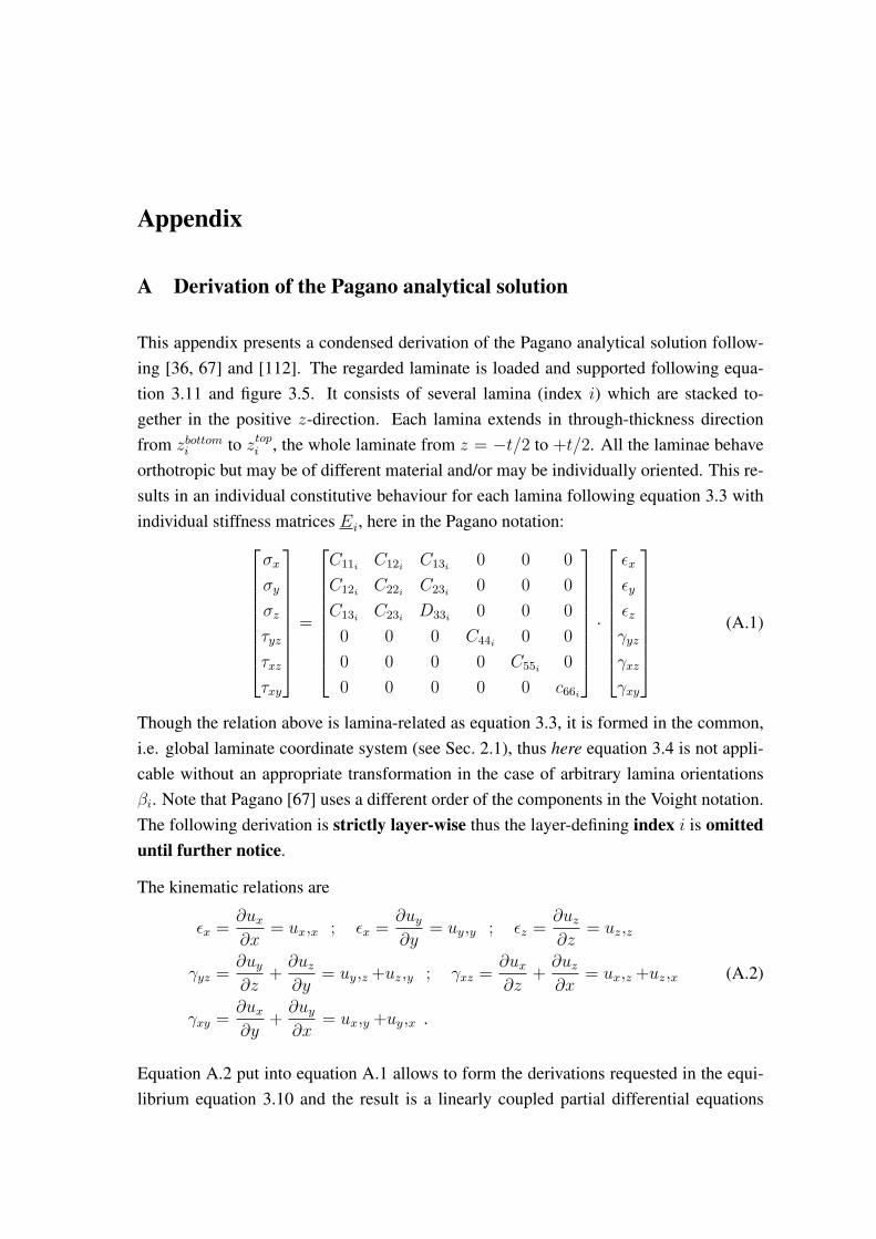
Appendix
A Derivation of the Pagano analytical solution
This appendix presents a condensed derivation of the Pagano analytical solution follow-ing [36, 67] and [112]. The regarded laminate is loaded and supported following equa-tion 3.11 and figure 3.5. It consists of several lamina (index 𝑖) which are stacked to-gether in the positive 𝑧-direction. Each lamina extends in through-thickness directionfrom 𝑧𝑏𝑜𝑡𝑡𝑜𝑚𝑖 to 𝑧𝑡𝑜𝑝𝑖 , the whole laminate from 𝑧 = −𝑡/2 to +𝑡/2. All the laminae behaveorthotropic but may be of different material and/or may be individually oriented. This re-sults in an individual constitutive behaviour for each lamina following equation 3.3 withindividual stiffness matrices 𝐸𝑖, here in the Pagano notation:⎡⎢⎢⎢⎢⎢⎢⎢⎢⎣
𝜎𝑥
𝜎𝑦
𝜎𝑧
𝜏𝑦𝑧
𝜏𝑥𝑧
𝜏𝑥𝑦
⎤⎥⎥⎥⎥⎥⎥⎥⎥⎦=
⎡⎢⎢⎢⎢⎢⎢⎢⎢⎣
𝐶11𝑖 𝐶12𝑖 𝐶13𝑖 0 0 0
𝐶12𝑖 𝐶22𝑖 𝐶23𝑖 0 0 0
𝐶13𝑖 𝐶23𝑖 𝐷33𝑖 0 0 0
0 0 0 𝐶44𝑖 0 0
0 0 0 0 𝐶55𝑖 0
0 0 0 0 0 𝑐66𝑖
⎤⎥⎥⎥⎥⎥⎥⎥⎥⎦⋅
⎡⎢⎢⎢⎢⎢⎢⎢⎢⎣
𝜖𝑥
𝜖𝑦
𝜖𝑧
𝛾𝑦𝑧
𝛾𝑥𝑧
𝛾𝑥𝑦
⎤⎥⎥⎥⎥⎥⎥⎥⎥⎦(A.1)
Though the relation above is lamina-related as equation 3.3, it is formed in the common,i.e. global laminate coordinate system (see Sec. 2.1), thus here equation 3.4 is not appli-cable without an appropriate transformation in the case of arbitrary lamina orientations𝛽𝑖. Note that Pagano [67] uses a different order of the components in the Voight notation.The following derivation is strictly layer-wise thus the layer-defining index 𝑖 is omitteduntil further notice.
The kinematic relations are
𝜖𝑥 =∂𝑢𝑥∂𝑥
= 𝑢𝑥,𝑥 ; 𝜖𝑥 =∂𝑢𝑦∂𝑦
= 𝑢𝑦,𝑦 ; 𝜖𝑧 =∂𝑢𝑧∂𝑧
= 𝑢𝑧,𝑧
𝛾𝑦𝑧 =∂𝑢𝑦∂𝑧
+∂𝑢𝑧∂𝑦
= 𝑢𝑦,𝑧 +𝑢𝑧,𝑦 ; 𝛾𝑥𝑧 =∂𝑢𝑥∂𝑧
+∂𝑢𝑧∂𝑥
= 𝑢𝑥,𝑧 +𝑢𝑧,𝑥
𝛾𝑥𝑦 =∂𝑢𝑥∂𝑦
+∂𝑢𝑦∂𝑥
= 𝑢𝑥,𝑦 +𝑢𝑦,𝑥 .
(A.2)
Equation A.2 put into equation A.1 allows to form the derivations requested in the equi-librium equation 3.10 and the result is a linearly coupled partial differential equations
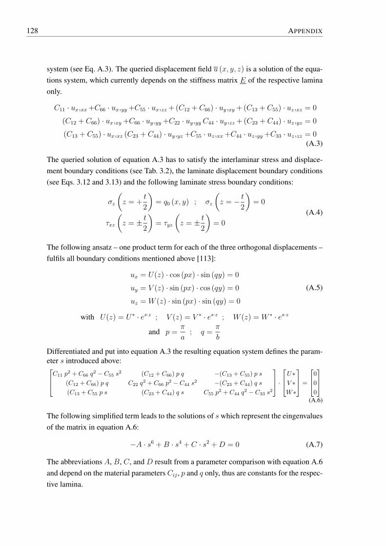
128 APPENDIX
system (see Eq. A.3). The queried displacement field 𝑢 (𝑥, 𝑦, 𝑧) is a solution of the equa-tions system, which currently depends on the stiffness matrix 𝐸 of the respective laminaonly.
𝐶11 ⋅ 𝑢𝑥,𝑥𝑥+𝐶66 ⋅ 𝑢𝑥,𝑦𝑦 +𝐶55 ⋅ 𝑢𝑥,𝑧𝑧 +(𝐶12 + 𝐶66) ⋅ 𝑢𝑦,𝑥𝑦 +(𝐶13 + 𝐶55) ⋅ 𝑢𝑧,𝑥𝑧 = 0
(𝐶12 + 𝐶66) ⋅ 𝑢𝑥,𝑥𝑦 +𝐶66 ⋅ 𝑢𝑦,𝑦𝑦 +𝐶22 ⋅ 𝑢𝑦,𝑦𝑦 𝐶44 ⋅ 𝑢𝑦,𝑧𝑧 +(𝐶23 + 𝐶44) ⋅ 𝑢𝑧,𝑦𝑧 = 0
(𝐶13 + 𝐶55) ⋅ 𝑢𝑥,𝑥𝑧 (𝐶23 + 𝐶44) ⋅ 𝑢𝑦,𝑦𝑧 +𝐶55 ⋅ 𝑢𝑧,𝑥𝑥+𝐶44 ⋅ 𝑢𝑧,𝑦𝑦 +𝐶33 ⋅ 𝑢𝑧,𝑧𝑧 = 0(A.3)
The queried solution of equation A.3 has to satisfy the interlaminar stress and displace-ment boundary conditions (see Tab. 3.2), the laminate displacement boundary conditions(see Eqs. 3.12 and 3.13) and the following laminate stress boundary conditions:
𝜎𝑧
(𝑧 = +
𝑡
2
)= 𝑞0 (𝑥, 𝑦) ; 𝜎𝑧
(𝑧 = − 𝑡
2
)= 0
𝜏𝑥𝑧
(𝑧 = ± 𝑡
2
)= 𝜏𝑦𝑧
(𝑧 = ± 𝑡
2
)= 0
(A.4)
The following ansatz – one product term for each of the three orthogonal displacements –fulfils all boundary conditions mentioned above [113]:
𝑢𝑥 = 𝑈(𝑧) ⋅ cos (𝑝𝑥) ⋅ sin (𝑞𝑦) = 0
𝑢𝑦 = 𝑉 (𝑧) ⋅ sin (𝑝𝑥) ⋅ cos (𝑞𝑦) = 0
𝑢𝑧 = 𝑊 (𝑧) ⋅ sin (𝑝𝑥) ⋅ sin (𝑞𝑦) = 0
(A.5)
with 𝑈(𝑧) = 𝑈∗ ⋅ 𝑒𝑠⋅𝑧 ; 𝑉 (𝑧) = 𝑉 ∗ ⋅ 𝑒𝑠⋅𝑧 ; 𝑊 (𝑧) = 𝑊 ∗ ⋅ 𝑒𝑠⋅𝑧
and 𝑝 =𝜋
𝑎; 𝑞 =
𝜋
𝑏
Differentiated and put into equation A.3 the resulting equation system defines the param-eter 𝑠 introduced above:⎡⎢⎣𝐶11 𝑝
2 + 𝐶66 𝑞2 − 𝐶55 𝑠
2 (𝐶12 + 𝐶66) 𝑝 𝑞 −(𝐶13 + 𝐶55) 𝑝 𝑠
(𝐶12 + 𝐶66) 𝑝 𝑞 𝐶22 𝑞2 + 𝐶66 𝑝
2 − 𝐶44 𝑠2 −(𝐶23 + 𝐶44) 𝑞 𝑠
(𝐶13 + 𝐶55 𝑝 𝑠 (𝐶23 + 𝐶44) 𝑞 𝑠 𝐶55 𝑝2 + 𝐶44 𝑞
2 − 𝐶33 𝑠2
⎤⎥⎦ ⋅
⎡⎢⎣𝑈∗𝑉 ∗𝑊∗
⎤⎥⎦ =
⎡⎢⎣000
⎤⎥⎦(A.6)
The following simplified term leads to the solutions of 𝑠 which represent the eingenvaluesof the matrix in equation A.6:
−𝐴 ⋅ 𝑠6 +𝐵 ⋅ 𝑠4 + 𝐶 ⋅ 𝑠2 +𝐷 = 0 (A.7)
The abbreviations 𝐴, 𝐵, 𝐶, and 𝐷 result from a parameter comparison with equation A.6and depend on the material parameters 𝐶𝑖𝑗 , 𝑝 and 𝑞 only, thus are constants for the respec-tive lamina.
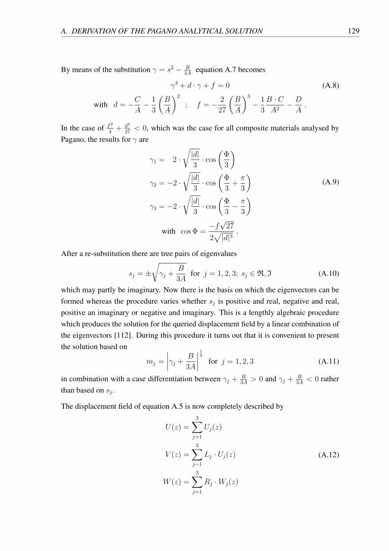
A. DERIVATION OF THE PAGANO ANALYTICAL SOLUTION 129
By means of the substitution 𝛾 = 𝑠2 − 𝐵3𝐴
equation A.7 becomes
𝛾3 + 𝑑 ⋅ 𝛾 + 𝑓 = 0 (A.8)
with 𝑑 = −𝐶𝐴
− 1
3
(𝐵
𝐴
)2
; 𝑓 = − 2
27
(𝐵
𝐴
)3
− 1
3
𝐵 ⋅ 𝐶𝐴2
− 𝐷
𝐴.
In the case of 𝑓2
4+ 𝑑3
27< 0, which was the case for all composite materials analysed by
Pagano, the results for 𝛾 are
𝛾1 = 2 ⋅√
∣𝑑∣3
⋅ cos(Φ
3
)𝛾2 = −2 ⋅
√∣𝑑∣3
⋅ cos(Φ
3+𝜋
3
)𝛾3 = −2 ⋅
√∣𝑑∣3
⋅ cos(Φ
3− 𝜋
3
) (A.9)
with cosΦ =−𝑓√27
2√∣𝑑∣3 .
After a re-substitution there are tree pairs of eigenvalues
𝑠𝑗 = ±√𝛾𝑗 +
𝐵
3𝐴for 𝑗 = 1, 2, 3; 𝑠𝑗 ∈ ℜ, ℑ (A.10)
which may partly be imaginary. Now there is the basis on which the eigenvectors can beformed whereas the procedure varies whether 𝑠𝑗 is positive and real, negative and real,positive an imaginary or negative and imaginary. This is a lengthly algebraic procedurewhich produces the solution for the queried displacement field by a linear combination ofthe eigenvectors [112]. During this procedure it turns out that it is convenient to presentthe solution based on
𝑚𝑗 =
∣∣∣∣𝛾𝑗 + 𝐵
3𝐴
∣∣∣∣ 12 for 𝑗 = 1, 2, 3 (A.11)
in combination with a case differentiation between 𝛾𝑗 + 𝐵3𝐴
> 0 and 𝛾𝑗 + 𝐵3𝐴
< 0 ratherthan based on 𝑠𝑗 .
The displacement field of equation A.5 is now completely described by
𝑈(𝑧) =3∑𝑗=1
𝑈𝑗(𝑧)
𝑉 (𝑧) =3∑𝑗=1
𝐿𝑗 ⋅ 𝑈𝑗(𝑧)
𝑊 (𝑧) =3∑𝑗=1
𝑅𝑗 ⋅𝑊𝑗(𝑧)
(A.12)
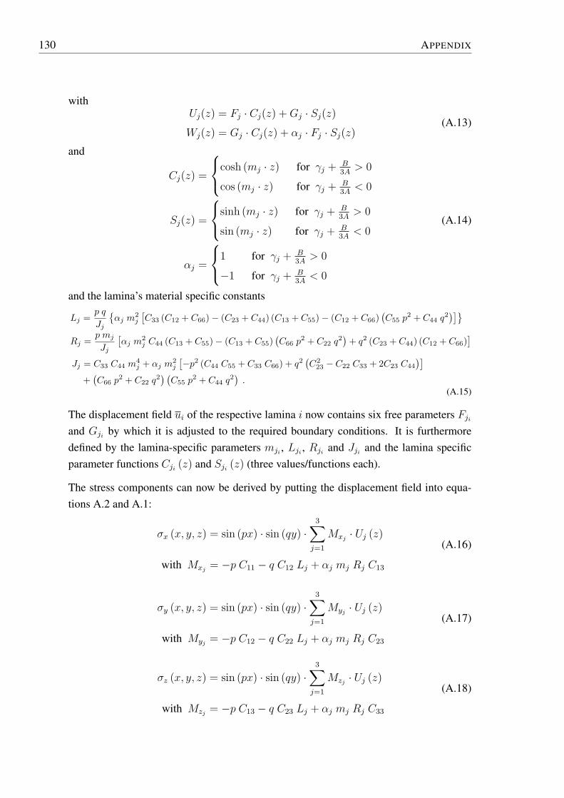
130 APPENDIX
with𝑈𝑗(𝑧) = 𝐹𝑗 ⋅ 𝐶𝑗(𝑧) +𝐺𝑗 ⋅ 𝑆𝑗(𝑧)𝑊𝑗(𝑧) = 𝐺𝑗 ⋅ 𝐶𝑗(𝑧) + 𝛼𝑗 ⋅ 𝐹𝑗 ⋅ 𝑆𝑗(𝑧)
(A.13)
and
𝐶𝑗(𝑧) =
⎧⎨⎩cosh (𝑚𝑗 ⋅ 𝑧) for 𝛾𝑗 + 𝐵3𝐴> 0
cos (𝑚𝑗 ⋅ 𝑧) for 𝛾𝑗 + 𝐵3𝐴< 0
𝑆𝑗(𝑧) =
⎧⎨⎩sinh (𝑚𝑗 ⋅ 𝑧) for 𝛾𝑗 + 𝐵3𝐴> 0
sin (𝑚𝑗 ⋅ 𝑧) for 𝛾𝑗 + 𝐵3𝐴< 0
𝛼𝑗 =
⎧⎨⎩1 for 𝛾𝑗 + 𝐵3𝐴> 0
−1 for 𝛾𝑗 + 𝐵3𝐴< 0
(A.14)
and the lamina’s material specific constants
𝐿𝑗 =𝑝 𝑞
𝐽𝑗
{𝛼𝑗 𝑚
2𝑗
[𝐶33 (𝐶12 + 𝐶66)− (𝐶23 + 𝐶44) (𝐶13 + 𝐶55)− (𝐶12 + 𝐶66)
(𝐶55 𝑝
2 + 𝐶44 𝑞2)]}
𝑅𝑗 =𝑝 𝑚𝑗
𝐽𝑗
[𝛼𝑗 𝑚
2𝑗 𝐶44 (𝐶13 + 𝐶55)− (𝐶13 + 𝐶55)
(𝐶66 𝑝
2 + 𝐶22 𝑞2)+ 𝑞2 (𝐶23 + 𝐶44) (𝐶12 + 𝐶66)
]𝐽𝑗 = 𝐶33 𝐶44 𝑚
4𝑗 + 𝛼𝑗 𝑚
2𝑗
[−𝑝2 (𝐶44 𝐶55 + 𝐶33 𝐶66) + 𝑞2(𝐶2
23 − 𝐶22 𝐶33 + 2𝐶23 𝐶44
)]+(𝐶66 𝑝
2 + 𝐶22 𝑞2) (
𝐶55 𝑝2 + 𝐶44 𝑞
2)
.(A.15)
The displacement field 𝑢𝑖 of the respective lamina 𝑖 now contains six free parameters 𝐹𝑗𝑖and 𝐺𝑗𝑖 by which it is adjusted to the required boundary conditions. It is furthermoredefined by the lamina-specific parameters 𝑚𝑗𝑖 , 𝐿𝑗𝑖 , 𝑅𝑗𝑖 and 𝐽𝑗𝑖 and the lamina specificparameter functions 𝐶𝑗𝑖 (𝑧) and 𝑆𝑗𝑖 (𝑧) (three values/functions each).
The stress components can now be derived by putting the displacement field into equa-tions A.2 and A.1:
𝜎𝑥 (𝑥, 𝑦, 𝑧) = sin (𝑝𝑥) ⋅ sin (𝑞𝑦) ⋅3∑𝑗=1
𝑀𝑥𝑗 ⋅ 𝑈𝑗 (𝑧)
with 𝑀𝑥𝑗 = −𝑝 𝐶11 − 𝑞 𝐶12 𝐿𝑗 + 𝛼𝑗 𝑚𝑗 𝑅𝑗 𝐶13
(A.16)
𝜎𝑦 (𝑥, 𝑦, 𝑧) = sin (𝑝𝑥) ⋅ sin (𝑞𝑦) ⋅3∑𝑗=1
𝑀𝑦𝑗 ⋅ 𝑈𝑗 (𝑧)
with 𝑀𝑦𝑗 = −𝑝 𝐶12 − 𝑞 𝐶22 𝐿𝑗 + 𝛼𝑗 𝑚𝑗 𝑅𝑗 𝐶23
(A.17)
𝜎𝑧 (𝑥, 𝑦, 𝑧) = sin (𝑝𝑥) ⋅ sin (𝑞𝑦) ⋅3∑𝑗=1
𝑀𝑧𝑗 ⋅ 𝑈𝑗 (𝑧)
with 𝑀𝑧𝑗 = −𝑝 𝐶13 − 𝑞 𝐶23 𝐿𝑗 + 𝛼𝑗 𝑚𝑗 𝑅𝑗 𝐶33
(A.18)
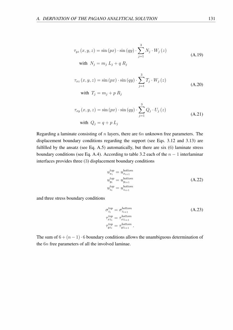
A. DERIVATION OF THE PAGANO ANALYTICAL SOLUTION 131
𝜏𝑦𝑧 (𝑥, 𝑦, 𝑧) = sin (𝑝𝑥) ⋅ sin (𝑞𝑦) ⋅3∑𝑗=1
𝑁𝑗 ⋅𝑊𝑗 (𝑧)
with 𝑁𝑗 = 𝑚𝑗 𝐿𝑗 + 𝑞 𝑅𝑗
(A.19)
𝜏𝑥𝑧 (𝑥, 𝑦, 𝑧) = sin (𝑝𝑥) ⋅ sin (𝑞𝑦) ⋅3∑𝑗=1
𝑇𝑗 ⋅𝑊𝑗 (𝑧)
with 𝑇𝑗 = 𝑚𝑗 + 𝑝 𝑅𝑗
(A.20)
𝜏𝑥𝑦 (𝑥, 𝑦, 𝑧) = sin (𝑝𝑥) ⋅ sin (𝑞𝑦) ⋅3∑𝑗=1
𝑄𝑗 ⋅ 𝑈𝑗 (𝑧)
with 𝑄𝑗 = 𝑞 + 𝑝 𝐿𝑗
(A.21)
Regarding a laminate consisting of 𝑛 layers, there are 6𝑛 unknown free parameters. Thedisplacement boundary conditions regarding the support (see Eqs. 3.12 and 3.13) arefulfilled by the ansatz (see Eq. A.5) automatically, but there are six (6) laminate stressboundary conditions (see Eq. A.4). According to table 3.2 each of the 𝑛− 1 interlaminarinterfaces provides three (3) displacement boundary conditions
𝑢𝑡𝑜𝑝𝑥𝑖 = 𝑢𝑏𝑜𝑡𝑡𝑜𝑚𝑥𝑖+1
𝑢𝑡𝑜𝑝𝑦𝑖 = 𝑢𝑏𝑜𝑡𝑡𝑜𝑚𝑦𝑖+1
𝑢𝑡𝑜𝑝𝑧𝑖 = 𝑢𝑏𝑜𝑡𝑡𝑜𝑚𝑧𝑖+1
(A.22)
and three stress boundary conditions
𝜎𝑡𝑜𝑝𝑧𝑖 = 𝜎𝑏𝑜𝑡𝑡𝑜𝑚𝑧𝑖+1(A.23)
𝜏 𝑡𝑜𝑝𝑥𝑧𝑖= 𝜏 𝑏𝑜𝑡𝑡𝑜𝑚𝑥𝑧𝑖+1
𝜏 𝑡𝑜𝑝𝑦𝑧𝑖= 𝜏 𝑏𝑜𝑡𝑡𝑜𝑚𝑦𝑧𝑖+1
.
The sum of 6+ (𝑛− 1) ⋅ 6 boundary conditions allows the unambiguous determination ofthe 6𝑛 free parameters of all the involved laminae.
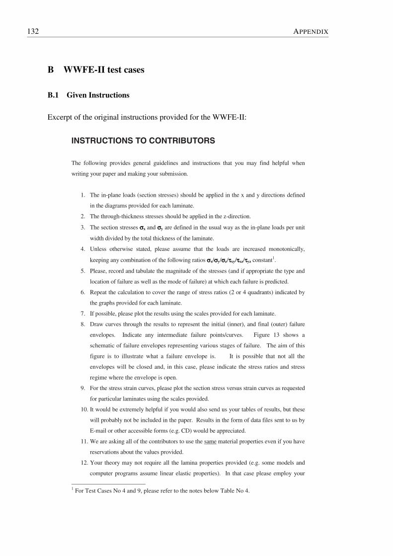
132 APPENDIX
B WWFE-II test cases
B.1 Given Instructions
Excerpt of the original instructions provided for the WWFE-II:
B. WWFE-II TEST CASES 133
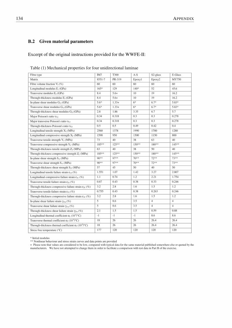
134 APPENDIX
B.2 Given material parameters
Excerpt of the original instructions provided for the WWFE-II:
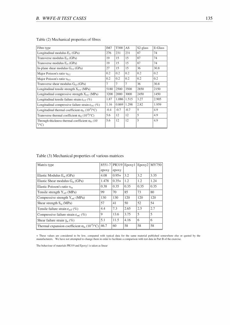
B. WWFE-II TEST CASES 135
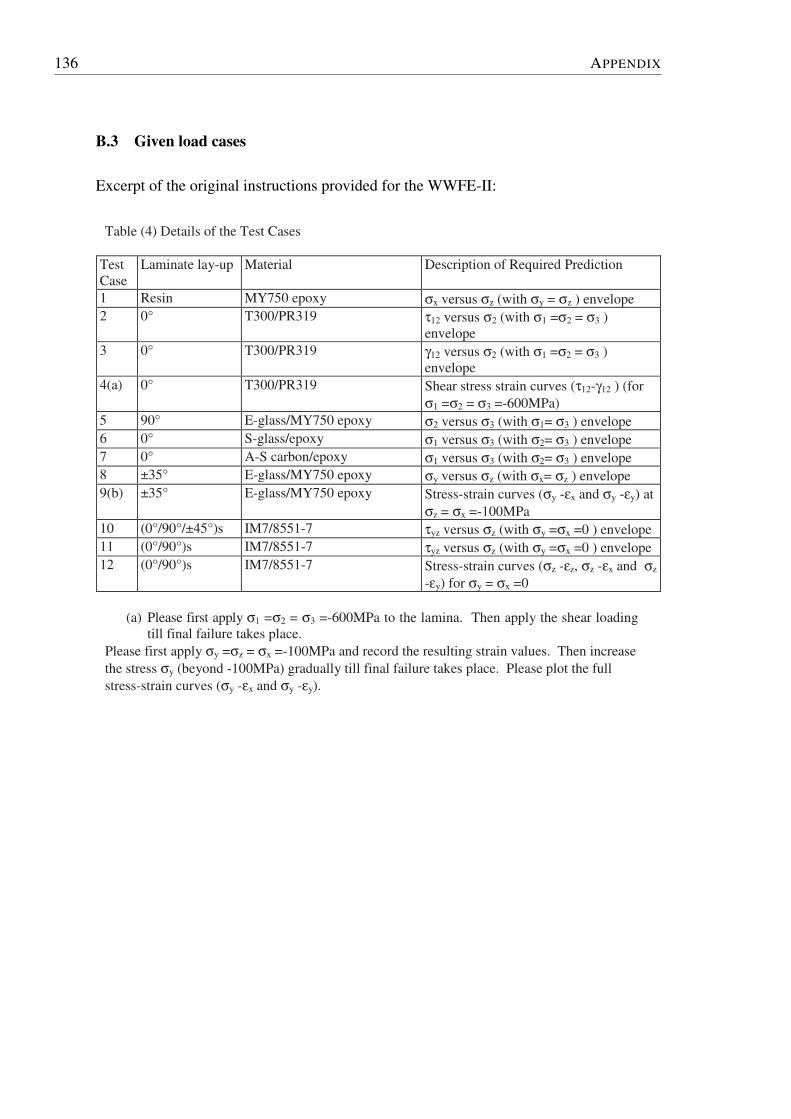
136 APPENDIX
B.3 Given load cases
Excerpt of the original instructions provided for the WWFE-II:
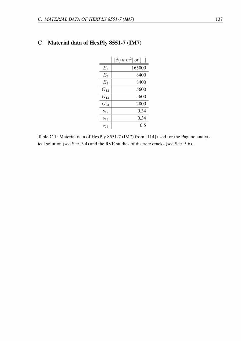
C. MATERIAL DATA OF HEXPLY 8551-7 (IM7) 137
C Material data of HexPly 8551-7 (IM7)
[𝑁/𝑚𝑚2] or [−]
𝐸1 165000𝐸2 8400𝐸3 8400𝐺12 5600𝐺13 5600𝐺23 2800𝜈12 0.34𝜈13 0.34𝜈23 0.5
Table C.1: Material data of HexPly 8551-7 (IM7) from [114] used for the Pagano analyt-ical solution (see Sec. 3.4) and the RVE studies of discrete cracks (see Sec. 5.6).

Bibliography
[1] G. Marsh. Composites lift off in primary aerostructures. Reinforced Plastics,48(4):22–27, 2004.
[2] M.J. Hinton, A.S. Kaddour, and P.D. Soden (Eds.). Failure Criteria in Fibre Rein-forced Polymer Composites: The World-Wide Failure Exercise. Elsevier, 2004.
[3] G. Busse, B.-H. Kroplin, and F.K.Wittel (Eds.). Damage and its Evolution in Fiber-Composite Materials. ISD Verlag, 2006.
[4] M. Knops. Analysis of Failure in Fiber Polymer Laminates: The Theory of AlfredPuck. Springer, 2008.
[5] A. Puck and H. Schurmann. Failure analysis of FRP laminates by means ofphysically based phenomenological models. Composites Science and Technology,58(7):1045–1067, 1998.
[6] A. Puck and H. Schurmann. Failure analysis of FRP laminates by means ofphysically based phenomenological models. Composites Science and Technology,62(12/13):1633–1662, 2002.
[7] A. Puck. Festigkeitsberechnung an Glasfaser/Kunststoff-Laminaten bei zusam-mengesetzter Beanspruchung: Bruchhypothese und schichtenweise Bruchanalyse.Kunststoffe, 59:780–787, 1969.
[8] ABAQUS Inc. ABAQUS Analysis User’s manual, v6.61 edition, 2006.
[9] H.M. Deuschle, W. Lutz, H. Gerger, and S. Schmauder. Simulation of Photoelas-ticity in a Glass Fibre Polymer Matrix Composite. In G. Busse, B.-H. Kroplin, andF.K.Wittel, editors, Damage and its Evolution in Fiber-Composite Materials. ISDVerlag, Stuttgart, 2006.
[10] H.M. Deuschle, F.K. Wittel, H. Gerhard, G. Busse, and B.-H. Kroplin. Investiga-tion of progressive failure in composites by combined simulated and experimentalphotoelasticity. Computational Materials Science, 38(1):1–8, 2006.
[11] F. Raischel, F. Kun, R.C. Hidalgo, and H.J. Herrmann. Statistical Damage Models:Fibre Bundle Models. In G. Busse, B.-H. Kroplin, and F.K.Wittel, editors, Damageand its Evolution in Fiber-Composite Materials. ISD Verlag, Stuttgart, 2006.
140 BIBLIOGRAPHY
[12] R.M. Jones. Mechanics of Composite Materials. McGawn-Hill, 1975.
[13] A. Puck. Zur Beanspruchung und Verformung von GFK-Mehrschichtverbund-Bauelementen – Teil 1: Grundlagen der Spannungs- und Verformungsanalyse.Kunststoffe, 57(4):284–293, 1967.
[14] L.J. Gibson and M.F. Ashby. Cellular Solids: Structure and Properties. CambridgeUniversity Press, 2nd edition, 1999.
[15] R. Talreja (Ed.). Comprehensive Composite Materials. Elsevier, 2000.
[16] J. Aboudi. Mechanics of Composite Materials – A Unified Micromechanical Ap-proach. Elsevier, 1991.
[17] M. Paley and J. Aboudi. Micromechanical Analysis of Composites by the Gener-alized Cells Model. Mechanics of Materials, 14:127–139, 2006.
[18] J. Lemaitre and J.L. Chaboche. Mechanics of Solid Materials. Cambridge Univer-sity Press, 1990.
[19] J. Lemaitre. A Course on Damage Mechanics. Springer, 2nd edition, 1996.
[20] D. Raabe. Computational Material Science: The Simulation of Material’s Mi-crostructures and Properties. Wiley-WCH, 1998.
[21] A. Puck. Should Fibre-Plastics Composites be designed with Strain or Stress Cri-teria. Kunststoffe - German Plastics, 82(5):34–38 & 431–434, 1992.
[22] B. Schlehofer and A. Mattern. Research of the suitability of GRP pipes for longdistance hot water transportation. Fernwarme Int., 10(4):194–198, 1981.
[23] J.W. Kopp. Contribution to the Stress and Strength Analysis of UnidirectionallyFibre Reinforced Plastics. PhD thesis, RWTH Aachen, Institut fur Kunststoffver-arbeitung (IKV), 2000.
[24] W. Michaeli, M. Knops, O. Fischer, and D. Eifel. Investigations on the fiber fracturebehaviour of carbon fiber reinforced plastics. In Proceedings of Intern. SAMPESymposium & Exhibition. Long Beach, CA, 2002.
[25] O. Fischer. Fibre Fracture Behaviour in Fibre Reinforced Plastics. PhD thesis,RWTH Aachen, Institut fur Kunststoffverarbeitung (IKV), 2003.
BIBLIOGRAPHY 141
[26] M. Mannigel. Influence of Shear Stresses on the Fibre Failure Behaviour in Car-bon Fibre Reinforced Plastics (CFRP). PhD thesis, RWTH Aachen, Institut furKunststoffverarbeitung (IKV), 2007.
[27] L.J. Hart-Smith. Predictions of a generalized maximum-shear-stress failure crite-rion for certain fibrous composite laminates. Composites Science and Technology,special issue 58:1179–1208, 1998.
[28] L.J. Hart-Smith. Predictions of the original and truncated maximum strain failuremodels for certain fibrous composite laminates. Composites Science and Technol-ogy, special issue 58:1151–1178, 1998.
[29] S. Lutze. Confocal laser scanning photoelasicity: Improvement of precision forquantitative photoelastic studies on model composite materials. SCANNING TheJ. of Scanning Microscopies, 23(4):273–278, 2001.
[30] F.K. Wittel, F. Kun, and H.J. Herrmann. Simulation of Damage and Fracture inComposites using a Dicrete Element Approach. In G. Busse, B.-H. Kroplin, andF.K.Wittel, editors, Damage and its Evolution in Fiber-Composite Materials. ISDVerlag, Stuttgart, 2006.
[31] S. Predak, H. Gerhard, I. Solodov, O. Bullinger, N. Davidson, and W. Lutz. Shortfibre reinforced thermoplastics. In G. Busse, B.-H. Kroplin, and F.K.Wittel, editors,Damage and its Evolution in Fiber-Composite Materials. ISD Verlag, Stuttgart,2006.
[32] D. Huybrechts. Ein erster Beitrag zur Verifikation des wirkebenebezogenenZwischenfaserbruchkriteriums nach Puck. Verlagshaus Mainz, Aachen, 1996.Technisch-wissenschaftlicher Bericht IKV, vol.44.
[33] R. Kruger. Delaminationswachstum in Faserverbundlaminaten. PhD thesis, Uni-versitat Stuttgart, ISD, 1996.
[34] S. Essebier. Berechnung dynamischer Delaminationsvorgange in Faserverbund-platten. PhD thesis, Universitat Stuttgart, ISD, 1999.
[35] M. D’Ottavio and M. Konig. Numerical Models for Delamination. In G. Busse, B.-H. Kroplin, and F.K.Wittel, editors, Damage and its Evolution in Fiber-CompositeMaterials. ISD Verlag, Stuttgart, 2006.
[36] N.J. Pagano (Ed.). Interlaminar Response of Composite Materials. Elsevier, 1989.
142 BIBLIOGRAPHY
[37] P.P. Camanho and C.G. Davila. Mixed-Mode Decohesion Finite Elements for theSimulation of Delamination in Composite Materials. NASA/TM, 211737(4):1–37,2002.
[38] ABAQUS Inc. ABAQUS Analysis User’s manual, v6.5 edition, 2004. Sec. 18.5.
[39] A. Puck. Festigkeitsanalyse von Faser-Matrix-Laminaten: Modelle fur diePraxis. Hanser Verlag, 1996. available online at http://www.klub.tu-darmstadt.de/forschung/download.php.
[40] J. Garbe and A. Puck. Erfahrungen mit Bruchkriterien an schwellend belastetenGFK-Drehfedern. Kunststoffe, 83(5):406–411, 1993.
[41] ZF Friedrichshafen AG. Focus on ultralight chassis. Technical report, 25.06.2009.press release.
[42] P. Gall. FE-Analyse einer Fahrzeugachse aus Faserverbund. Master’s thesis, ISDUniveritat Stuttgart, 2009.
[43] S. Fell, T. Gull, R. Immel, T. Schutz, V. Schultheis, M. Shubert, and W. Oelerich.CAE-Prozesskette zur Festikeits- und Crashanalyse von Hochdrucktanks aus nass-gewickeltem Faser-Kunststoff-Verbund. NAFEMS Magazin, 9(1):20–33, 2008.
[44] I.M. Daniel and O. Ishai. Engineering Mechanics of Composite Materials. OxfordUniversity Press, 1994.
[45] A. Puck and M. Mannigel. Physically based nonlinear stress-strain relations for theinter-fibre fracture analysis of FRP laminates. Composites Science and Technology,67(9):1955–1964, 2007.
[46] M. D’Ottavio. Advanced Hierarchical Models of Multilayered Plates and Shells In-cluding Mechanical and electrical Interfaces. PhD thesis, Universitat Stuttgart, In-stitut fur Statik und Dynamik der Luft- und Raumfahrtkonstruktionen (ISD), 2008.
[47] K. Washizu. Variational Methods in Elasticity and Plasticity. Pergamon Press, 3rdedition, 1982.
[48] A.J.M. Spencer. Deformation of Fibre-reinforced Materials. Oxford UniversityPress, 1972.
[49] E. Carrera. 𝐶0𝑧 -Requirements – models for the two-dimensional analysis of multi-
layered structures. Composite Structures, 37:373–383, 1997.
BIBLIOGRAPHY 143
[50] J.N. Reddy. Energy Principles and Variational Methods in Applied Mechanics.John Wiley, 2002.
[51] H. Kraus. Thin Elastic Shells. John Wiley & Sons, 1967.
[52] E. Reissner. The effect of transverse shear deformation on the bending of elasticplates. J. of Applied Mechanics, 12:69–76, 1945.
[53] R.D. Mindlin. Influence of rotatory inertia and shear on fluxural vibrations ofisotropic, elastic plates. J. of Applied Mechanics, 18:31–38, 1951.
[54] Y.M. Ghugal and R.P. Shimpi. A review of refined shear deformation theories ofisoropic and anisotropic laminated plates. J. of Reinforced Plastics and Compos-ites, 21:775–813, 2002.
[55] K.P. Saldatos. A redifined laminated plate and shell theory with applications. Jour-nal of Sound and Vibration, 144:109–129, 1991.
[56] P.R. Hildebrand, E. Reissner, and G.B. Thomas. Notes on the foundations of theoryof small displacements of orthotropic shells. National Advisory Commitee forAeronautics, 1949. Technical Report 1833.
[57] K.H. Lo, R.M. Christensen, and E.M. Wu. A high-order theory of plate defor-mation – Part 1: Homogenious plates, Part 2: Laminated Plates. J. of appliedMechanics, 44:663–668 & 669–676, 1978.
[58] A.K. Noor and W.S. Burton. Assessment of computational models for multilayeredshells. Applied Mechanics Review, 43:67–97, 1990.
[59] J.N. Reddy and D.H. Robbins Jr. Theories and computational models for compositelaminates. Applied Mechanics Review, 47:147–169, 1994.
[60] E. Carrera. An assessment of mixed and classical theories on global and localresponse of multilayered orthotropic plates. Composite Structures, 50:183–198,2000.
[61] K.H. Lo, R.M. Christensen, and E.M. Wu. Stress solution determination for highorder plate theory. Int. J. of Solids and Structures, 14:655–662, 1978.
[62] J.M. Whitney. The effect of transverse shear deformation on the bending of lami-nated plates. J. of Composite Material, 3:534–547, 1969.
[63] E. Carrera. Historical review of zig-zag theories for multilayered plates and shells.Applied Mechanics Review, 56:287–308, 2003.
144 BIBLIOGRAPHY
[64] S.A. Ambartsumyan. Theory of Anisotropic Plates. Technomic Publishing Com-pany, 1970.
[65] E. Reissner. On a certain mixed variational theorem and a proposed application.Int. J. of Numerical Methods in Engineering, 20(7):1366–1368, 1984.
[66] E. Reissner. On a mixed variational theorem and on shear deformable plate theory.Int. J. of Numerical Methods in Engineering, 23(2):193–198, 1986.
[67] N.J. Pagano. Exact Solutions for Rectangular bidirectional Composites and Sand-wich Plates. Journal of Composite Materials, 4:20–34, 1969.
[68] K. Girkmann. Flachentragwerke. Springer, 1946.
[69] A.S. Kaddour and M.J. Hinton. 3D properties of unidirectional composite laminaeand test problems used in WWFE-II. to be published.
[70] W. Michaeli, D. Huybrechts, and M. Wegener. Dimensionieren mit Faserverbund-kunststoffen. Hanser, 1995.
[71] J.R. Vinson and R.L. Sierakowski. The Behaviour of Composite Materials. Marti-nus Nijhoff Publishers, 1986.
[72] S.W. Tsai. Composite Design – Think Composites. Dayton, 1988.
[73] K. Moser. Faser-Kunststoff-Verbund. VDI-Verlag, 1992.
[74] R. Hill. Elastic properties of reinforced solids: Some theoretical principles. J. ofthe Mechanics and Physics of Solids, 11:352–372, 1963.
[75] S. Nemat-Nasser and M. Hori. Micromechanics: Overall properties of heteroge-neous materials. North-Holland, 1998.
[76] M. D’Ottavio, F.K. Wittel, and J.Reiser. Mechanisms based Toolbox: PrototypicalImplementation of Tools. In G. Busse, B.-H. Kroplin, and F.K.Wittel, editors,Damage and its Evolution in Fiber-Composite Materials. ISD Verlag, Stuttgart,2006.
[77] M. Willamowski. Untersuchung des Degradationsverhaltens von unidirektionalverstarkten Faserverbundschichten im Fall von Zwischenfaserbruchen. Master’sthesis, Institut fur Statik und Dynamik der Luft- und Raumfahrtkonstruktionen(ISD), Universitat Stuttgart, 2008.
BIBLIOGRAPHY 145
[78] J. Loose. Bestimmung der mechanischen Eigenschaften inhomogener Werkstoffemit Hilfe des Konzeptes der reprasentativen Volumenelemente. Master’s thesis, In-stitut fur Statik und Dynamik der Luft- und Raumfahrtkonstruktionen (ISD), Uni-versitat Stuttgart, 2007.
[79] P. Ludwik. Elemente der technologischen Mechanik. J. Springer, 1909.
[80] L. Issler, H. Ruoß, and P. Hafele. Festigkeitslehre – Grundlagen. Springer, 2ndedition, 2003.
[81] S.W. Tsai and E. Wu. A General Theory of Strength for Anisotropic Materials.Journal of Composite Materials, 5(1):58–80, 1971.
[82] K.S. Liu and S.W. Tsai. A Progressive quadratic failure criterion for a laminate –Part A. Composites Science and Technology, 58:1023–1032, 1998.
[83] M. Knops. Die wirkebenenbezogenen Bruchkriterien von Puck. In Proc. of Di-mensionieren mit Faserverstarkten Kunststoffen – IKV Fachtagung zur Kunststof-fverarbeitung. Aachen, 2008.
[84] C.A. Coulomb. Sur une Application des Regles de Maximis et Minimis a quelquesProblemes de Statique relatives a l’Architecture. In Memoires de Mathematique etde Physique: Anne 1773. Academie Royal des Sciences par divers Savans, Paris,France, 1776.
[85] O. Mohr. Welche Umstande bedingen die Elastizitatsgrenze und den Bruch einesMaterials. Zeitschrift des VDI, 24(45/46):1524–1541 & 1572–1577, 1900.
[86] B. Paul. A Modification of the Coulomb-Mohr Theory of Fracture. Journal ofApplied Mechanics, 28:259–268, 1961.
[87] G. Lutz. The Puck theory of failure in laminates in the context of the new guidelineVDI2014 Part 3. In Proceedings of Conference on Damage in Composite Materi-als. Stuttgart, 2006. available online at http://www.ndt.net/v11n12.htm.
[88] VDI 2014/3. Development of Fibre-Reinforced Plastics components: Analysis.Technical report, Verein Deutscher Ingenieure e.V., Dusseldorf, 2006.
[89] A. Puck, J. Kopp, and M. Knops. Guidelines for the determination of the parame-ters in Puck’s action plane strength criterion. Composites Science and Technology,62(3 & 9):371–378 & 1275, 2002.
146 BIBLIOGRAPHY
[90] P.P. Camanho, P. Maimı, and C.G. Davila. Prediction of size effects in notched lam-inates using continuum damage mechanics. Composites Science and Technology,67:2715–2727, 2007.
[91] I.V. Papadopoulos. Critical plane approaches in high-cycle fatigue: On the defini-tion of amplitude and mean value of shear stress acting on the critical plane. Fatigueand Fracture of engineering Materials and Structures, 21(3):269–285, 1998.
[92] Institut fur Kunststoffverarbeitung (IKV), RWTH Aachen. COMPOSITOR: Hilfs-mittel zur Analyse von Laminaten aus Faserverbundkunststoffen, 3.0 edition, 2007.
[93] S. Weihe, B. Kroplin, and R. de Borst. Classification of smeared crack modelsbased on material and structural properties. Int. Journal of Solids and Structures,35(12):1289–1308, 1998.
[94] L. Lambrecht. Numerische Experimente zur Analyse der Einflussgroßen auf dieDegradation von mehrschichtigem GFK-Laminat. Master’s thesis, Institut fur Kun-ststoffverarbeitung (IKV), RWTH Aachen, 2003.
[95] M. Knops. Gradual failure process in fibre/polymer laminates. PhD thesis, RWTHAachen, Institut fur Kunststoffverarbeitung (IKV), 2003.
[96] M. Knops and C. Bogle. Gradual failure process in fibre/polymer laminates. Com-posites Science and Technology, 66(5):616–625, 2006.
[97] A. Matzenmiller, J. Lubliner, and R.L. Taylor. A constitutive model for anisotropicdamage in fiber-composites. Mechanics of Materials, 20:125–152, 1995.
[98] A. Puck and H.M. Deuschle. A simple physically based degradation model forFRP-UD laminate after onset of cracking caused by inter fibre fracture. 2009.short note submitted to Composites Science and Technology.
[99] H. Schurmann. Konstruieren mit Faser-Kunststoff-Verbunden. Springer, 2nd edi-tion, 2007.
[100] A.L. Highsmith and K.L. Reifsnider. Damage in Composite Materials. In K.L.Reifsnider, editor, ASTM STP 775. American Society for Testing and Materials,Philadelphia, PA, 1982.
[101] R. Talreja. Transverse cracking and stiffness reduction in cross ply laminates ofdifferent matrix toughness. Journal of Composite Materials, 26:1644–1663, 1992.
BIBLIOGRAPHY 147
[102] J.W. Hoover, D. Kujawski, and F. Ellyin. Transverse cracking of symmetric andunsymmetric glass-fibre/epoxy-resin laminates. Composites Science and Technolo-gie, 57:1513–1526, 1997.
[103] C. Li, F. Ellyin, and A. Wharmby. On matrix crack saturation in composite lami-nates. Composites Part B. Engineering, 34:473–480, 2003.
[104] E. Hinton and D.R.J. Owen. An introduction to finite element computations. Piner-idge Press, 1981.
[105] G.D. Smith. Numerical solution of partial differential equations: finite differencemethods. Oxford University Press, 1985.
[106] K.H. Huebner, D.L. Dewhirst, D.E. Smith, and T.G. Byrom. The Finite ElementMethod for Engineers. John Wiley & Sons, 4th edition, 2001.
[107] D. Quabis. FEM-based Failure Analysis of UD Composites following Puck. Mas-ter’s thesis, Institut fur Statik und Dynamik der Luft- und Raumfahrtkonstruktionen(ISD), Universitat Stuttgart, 2009.
[108] T. Lindemann. Analytische Verfeinerungen der Puckschen Versagenshypothesenfur Faserverbundmaterial. Master’s thesis, Institut fur Statik und Dynamik derLuft- und Raumfahrtkonstruktionen (ISD), Universitat Stuttgart, 2009.
[109] H.M. Deuschle and B.-H. Kroplin. FE Implementation of Puck’s Failure Theoryfor Fibre Reinforced Composites under 3D-Stress. 2009. submitted to CompositesScience and Technology.
[110] F.K.Wittel. Diskrete Elemente - Modelle zur Bestimmung der Festigkeitsevolutionin Verbundwerkstoffen. PhD thesis, Universitat Stuttgart, ISD, 2006.
[111] P.J. Hine, R.A. Duckett, A.S.Kaddour, M.J.Hinton, and G.M. Wells. The effectof hydrostatic pressure on the mechanical properties of glass fibre/epoxy unidirec-tional composites. Composites Part A, 36:279–289, 2005.
[112] M. Hahn. 3D Spannungsanalyse von Faserverbundlaminaten: Vergleich vonFiniten Volumen- und Schalenelementen mit der analytischen Losung nachPagano. Master’s thesis, Institut fur Statik und Dynamik der Luft- und Raum-fahrtkonstruktionen (ISD), Universitat Stuttgart, 2008.
[113] C. Navier. Memoires sur les lois de l’equilibre et du mouvement des corps solideselastiques. Mem. Acad. Sci. Inst. Fr., 7:375–393, 1824.

148 BIBLIOGRAPHY
[114] Hexcel Company. Product Data HexPly 8551-7 (IM7).http://www.hexcel.com/NR/rdonlyres/C7264B73-64EE-4CA1-ADC2-5573E6E98FB4/0/HexPly 8551 7 us.pdf, 2009.
Vita
Particulars:
Name Heiko Matthias DeuschleDate / place of birth July 18, 1977 in KarlsruheMarital status marriedNationality German
Schools:
1984 – 1988 Pestalozzi Grundschule Rheinstetten1988 – 1997 Walahfrid-Strabo-Gymnasium Rheinstetten
Allgemeine Hochschulreife 05/1997
Civilian Service:
1997 – 1998 Arbeiter-Samariter-Bund Rheinstetten
Studies:
1998 – 2004 Aero- and astronautics engineering at theUniversitat Stuttgart
Diplom-Ingenieur aer. 09/2004Doktor-Ingenieur aer. 09/2010
Professional activity:
since 09/2004 Research associate with the Institut furStatik und Dynamik der Luft- undRaumfahrtkonstruktionenat the Universitat Stuttgart
since 01/2007 Teaching assistant with the Institut furStatik und Dynamik der Luft- undRaumfahrtkonstruktionenat the Universitat Stuttgart
since 09/2010 FEM Calculation Engineer withKolt Engineering,Boblingen, Germany


ISBN 3-930683-99-7
![A Review on Natural Fibre Reinforced Polymer Composites · natural fibre reinforced polymer composites increase with increasing fibre loading. Khoathane et al. [1] found that the](https://img.pdfslide.us/doc/110x75/5e21837fc2d50e18910e61ca/a-review-on-natural-fibre-reinforced-polymer-composites-natural-fibre-reinforced.jpg)