3D Computer Graphics

3D computer graphics 3D computer graphics software 3D model 3D projection 3DcAmbient occlusion Back-face culling Beam tracing Bilinear filtering Bloom (shadereffect) Bounding volume Box modeling Bui Tuong Phong Bump mapping Carmack'sReverse Catmull-Clark subdivision surface Cel-shaded animation Cg programminglanguage Clipmap COLLADA Comparison of Direct3D and OpenGL Cone tracingConstructive solid geometry Conversion between quaternions and Euler anglesCornell Box Crowd simulation Cube mapping Diffuse reflection Digital puppetryDilution of precision (computer graphics) Direct3D Displacement mapping Distancefog Draw distance Euler boolean operation Flat shading Forward kinematicanimation Fragment (computer graphics) Gelato (software) Geometric modelGeometry pipelines Geometry Processing GLEE GLEW Glide API Globalillumination GLSL GLU GLUI Gouraud shading Graphics pipeline Hidden lineremoval Hidden surface determination High dynamic range imaging High dynamicrange rendering High Level Shader Language Humanoid Animation Image basedlighting Image plane Inverse kinematic animation Inverse kinematics IrregularZ-buffer Isosurface Joint constraints Lambert's cosine law Lambertian reflectanceLevel of detail (programming) Low poly MegaTexture Mesa 3D Metaballs Metropolislight transport Micropolygon Mipmap Morph target animation Motion captureNewell's algorithm Normal mapping Open Inventor OpenGL OpenGL ES OpenGLUtility Toolkit OpenGL++ OpenRT Painter's algorithm Parallax mapping Particlesystem Path Tracing Per-pixel lighting Perlin noise Phong reflection model Phongshading Photon mapping Photorealistic (Morph) PLIB Polygon (computer graphics)Polygon mesh Polygonal modeling Pre-rendered Precomputed Radiance TransferProcedural generation Procedural texture Pyramid of vision Qualitative invisibilityQuaternions and spatial rotation Radiosity Ray casting Ray tracing Ray tracinghardware Reflection mapping Render layers Rendering (computer graphics)Retained mode S3 Texture Compression Scanline rendering Scene graph ShaderShading language Shadow mapping Shadow volume Silhouette edge Solidmodelling Specular highlight Specularity Stencil buffer Stencil shadow volumeSubdivision surface Subsurface scattering Surface caching Surface normalSynthespian Tao (software) Texel (graphics) Texture filtering Texture mappingTransform and lighting Unified lighting and shadowing Utah teapot UV mappingVertex Viewing frustum Volume rendering Volumetric lighting Voxel W-bufferingZ-buffering Z-fighting

#Clipping #Display #fn_1 #fn_1_back #Lighting #Modeling transformation #Projection transformation #ref_cgHome #ref_Debevec97 #ref_Debevec98 #ref_fxcomp #ref_gelatoHome #ref_glslangResources #ref_glslangSamplers#ref_glslangSpec #ref_glslangUniforms #ref_multitexturing #ref_nvdeveloper #ref_oldFrag #ref_oldVtx #ref_pipeline #ref_RMSpec #ref_stages #Scan conversion or rasterization #Texturing or shading #Viewing transformation.kkrieger 16-bit 1940s 1966 1968 1971 1972 1975 1977 1983 1984 1985 1990s 1994 1996 1999 19th century 2000 2002 2003 2004 2005 2006 2006-05-16 20th century 24-bit 27 October 2D computer graphics 2D geometric model 3-Dcomputer graphics 3-sphere 32-bit 3D animation 3D computer graphics 3D computer graphics software 3D computer graphics#Modelling 3D display 3D geometric model 3D geometry 3D graphics 3D graphics card 3D model 3Dmodeler 3D modeling 3D modelling 3d motion controller 3D projection 3D rendering 3d scanner 3D Studio 3D Studio Max 3Dc 3dfx 3Dlabs 4D 6 March 6DOF 8-bit AABB Aberration_in_optical_systems absorption absorption (optics)Academy Awards acceleration accuracy and precision ACIS ACM Press ACM Transactions on Graphics acquisition Act of War: High Treason Activision actor Actual state Ada programming language Adobe Illustrator AdobePremiere Pro Adobe Systems AfterBurn Age of Empires III AGL (API) Aki Ross algorithm algorithmic algorithms Alias Systems Corporation aliasing Allegro library almost everywhere Alpha blending alpha channel Alpha compositingAmapi(software) ambient light ambient occlusion Anaglyph image analysis anatomical position anatomy angle Anim8or Animation animation control Animation#Styles and techniques of animation animator anime anisotropicAnisotropic filtering Anisotropic_Filtering Anthony A. Apodaca anthropomorphism Anti-Aliasing Antialiasing API Apple Computer Appleseed Application programming interface application software applied mathematics arcadegame Architecture Review Board array Art of Illusion Arthur Appel artifact (observational) Artificial intelligence artist Ascendant assembly language assembly modelling Association for Computing Machinery associativity astrologyATI ATI Technologies ATI_Technologies Atomic Betty August 23 August 9 Auto Modellista AutoCAD Autodesk Autodesk_Media_and_Entertainment Autodesk_Media_and_Entertainment#Combustion autodessys, Inc. AutoQ3Dautostereogram AUX Avid Technology avionics Axis_of_rotation B-spline Back-face_culling bandwidth Barycentric coordinates (mathematics) batch BBC beam tracing Beauty and the Beast (1991 film) BeOS Bet on SoldierBeyblade: The Movie - Fierce Battle Bezier curve bi-directional path tracing Bicubic interpolation Bidirectional Reflectance Distribution Function bilinear filtering bilinear interpolation binary space partitioningBinary_space_partitioning binding (computer science) binocular biomedical computing Bioshock Birch bit bitmap bitmap textures Black & White (game) black body Blender (software) Blinn-Phong shading Bloom (shader effect)BMRT Bomberman Generation Bomberman Jetters bone Boolean Boundary representation bounding cylinder bounding sphere bounding volume bounding volume hierarchies box modeling box splines brain branch Brazil r/sBresenham's line algorithm Brian Paul brightness BRL-CAD Brothers in Arms: Earned in Blood Brothers In Arms: Hell's Highway Brothers in Arms: Road to Hill 30 Bryce (software) BSD license BSP tree Buck 65 buffer buffer(computer science) Bugs Bunny Bui Tuong Phong bump mapping bumpmapping Butterfly byte C programming language C Sharp programming language C++ C4 Engine cache cache coherency cache memory CAD CAD#Historycalculation calculus Call of Duty 2 Caltech CAM Canada's Worst Driver Carbon (API) cardinal point (optics) Carmack's Reverse Carrara (software) cartesian coordinate system cartoon Cass Everitt casting cat CATIA Catmull-Clarksubdivision surface Caustic (optics) Caustic_(optics) caustics Cel Damage Cel-shaded_animation Cell (microprocessor) celluloid cellulose acetate central processing unit CG Cg programming language CGL change state Characteranimation Charge-coupled device Charts on SO(3) chemistry chirality chromatic aberration chrominance Cinema 4D cinematography CinePaint Circle circumference ClanLib Class of the Titans clean room design Clifford algebra ClipMapping Clipping (computer graphics) Clipping_(computer_graphics) Cocoa (API) CODE V collinear collision detection color color buffer comic book Comm. ACM Command & Conquer: Tiberian series Commutative operationCompact disc Comparison of Direct3D and OpenGL compiler Compiz complement (set theory) complex analysis complex number complex polygon Component Object Model composite pattern compositing Compression artifactscomputation computational fluid dynamics computational geometry Computational_geometry computed axial tomography Computed tomography computer Computer Aided Design computer and video games Computer animationcomputer cluster computer display computer file computer game computer games computer generated image computer graphics Computer hardware Computer History Museum Computer keyboard Computer mouse computerprogram Computer programming computer science computer software computer storage Computer-aided design Computer-aided design#Capabilities computer-aided manufacturing computer-generated imagery concave cone(solid) Cone tracing Conjugacy_class#Conjugacy_as_group_action consortium constraints Constructive solid geometry continuous function contrast ratio conversion between quaternions and Euler angles convex convex hullconvex set coordinate coordinate rotation Coordinate system Coordinate_rotation#Three_dimensions coordinates CorelDRAW Cornell Box Cornell University cosine Cosmo 3D Counter-Strike: Source covering mapCovering_space#Elementary_properties CPU Crazyracing Kartrider Creative Labs Cross platform cross product cross-platform crowd psychology Crysis Crystal Space Crytek cube cube (geometry) cube map cube mapping cuboidcurve curvilinear coordinates cut scene cyclic permutation cylinder cylinder (geometry) D.I.C.E. D3DX Daily Planet (TV series) Dark Cloud 2 Darwyn Peachey Data (computing) data compression data structure datatype David S. ElbertDay of Defeat: Source decal December 24 Decimal separator degrees of freedom (engineering) Delilah and Julius Dell, Inc. Delta Force (computer game) Demo (computer programming) demo effect Demo effects demoscene densitydepth buffer depth of field depth perception Deus Ex: Invisible War device driver diameter diffraction diffuse inter-reflection diffuse interreflection Diffuse reflection diffusion digital digital camera digital content creation DigitalEquipment Corporation digital image Digital image processing digital images digital puppetry digital signal processing Dilution of precision (computer graphics) dimension Dimensionless number direct illumination Direct3DDirect3D vs. OpenGL DirectDraw DirectDraw Surface directly proportional DirectX DirectX Graphics Disney's California Adventure dispersion (optics) displacement mapping Display Generator distance fog Distance_fog distributedray tracing Doctor of Science Doctor Who dodecahedron Doo-Sabin Doom Doom 3 Doom engine dot product Dragon Ball Z: Budokai 2 Dragon Ball Z: Budokai 3 Dragon Ball Z: Budokai Tenkaichi Dragon Booster Dragon Quest VIIIDTP Duck Dodgers Duke Nukem 3d Duke Nukem Forever dust DVD dxf DXT5 dynamic link library dynamic range dynamical simulation earth science edge (graph theory) edge modeling educational film Edwin Catmull EidosInteractive elbow Elite (computer game) ellipse Elmsford, New York embedded device Emergent behavior emission spectrum emulate Enemy Territory: Quake Wars energy Engineering Engineering drawing entertainmentenvironment map environment mapping environmental audio extensions Eovia Epic Games Epic Megagames Eric Lengyel Eric Veach Euclidean geometry Euclidean space Euler angle Euler angles Euler characteristic Evans &Sutherland execute buffer Exile (BBC computer game) Exposure (photography) extrusion eye E³ F. Kenton Musgrave F.E.A.R. Facet Facial motion capture fad Fahrenheit graphics API Fairly OddParents Family Guy Far Cry Far CryInstincts: Predator Farbrausch FarCry Fear Effect February 2 field of view file format film Film editing Final Cut Pro Final Fantasy: The Spirits Within Final gathering Final-Render Finding Nemo Finger protocol Finite difference finiteelement Finite element analysis Finite element method finite state machine Finite_element_analysis FireGL first-person shooter fisheye lens Fixed-point Fixed-point arithmetic flat shading flight dynamics Flight simulator floatingpoint Floating point unit FLOPS FLTK fluid flow FMV game fog form factor (radiative transfer) formZ Fortran 90 forward kinematic animation FOURCC fractal Fractal landscape Fraction (mathematics) fragment Fragment (computergraphics) Frame (film) frame buffer Frame rate framebuffer frames per second Frank Crow free software Freeform surface Freeform surface modelling freeglut Frontier (computer game) frustum full motion video full screen effectFull_motion_video function (mathematics) function (programming) function composition functional programming Funky Cops Futurama FXT1 G.I. Joe: Sigma 6 Game Developers Conference game physics game programmerGameCube gamma correction gamma radiation gamut Gaussian distribution Gears of War GeForce GeForce 2 GeForce 256 GeForce 6 GeForce 6 Series GeForce 7 GeForce 7 Series GeForce 8 Series GeForce FX GeForce2 GeForce3GeForce4 Gelato (software) Genus (mathematics) Geologic modeling geometric geometric primitive geometric space geometrical optics geometry geophysics Ghost in the Shell: S.A.C. 2nd GIG Ghost in the Shell: Stand AloneComplex gigabytes glass cockpit GLEE GLEW Glide API Global illumination glossy GLSL GLU glucose transporter GLUI GLUT GLX GNU General Public License GNU GPL GoForce Gollum Google Earth gouraud shading GPGPUGPU gradient Grand Theft Auto (game) Grand Theft Auto (series) Grand Theft Auto 3 granite granularity graph theory graphic art Graphics graphics card Graphics cards graphics hardware Graphics pipeline graphics processing unitGraphics_cards Graphics_processing_unit gravity grayscale green Greg Ward Gregory Ward group (mathematics) group action group dynamics group theory GTK+ GUI Gundam Seed Gungrave half precision Half-Life 2 Half-Life 2:Episode One Half-Life 2: Lost Coast Halo (optical phenomenon) Halo 2 hardware hardware acceleration Harvest Moon: Save the Homeland He-Man and the Masters of the Universe (2002) heat heat transfer heightfield heightmaphemicube Henri Gouraud (computer scientist) Henrik Wann Jensen heuristic (computer science) Hewlett-Packard Hexagon(software) hidden face removal hidden line removal Hidden surface determinationHidden_surface_determination high dynamic range imaging High dynamic range rendering High Level Shader Language high-definition highlight History of 3D Graphics HLSL homogeneous coordinates Hoops3D horoscope HotWheels Highway 35 World Race Houdini (software) Hounsfield_scale HSV color space HTML hue human eye Huxley MMOFPS hypotenuse I-DEAS Ian Bell IBM icosahedron Id Software IEEE Transactions on Computers IHV illusionimage image compression image order image plane image processing image resolution image-based lighting Image_compression immediate-mode rendering implementation Implicit function implicit model implicit surface impulse(physics) in-joke infinitesimal Initial D injection molding Injection moulding Innocence: Ghost in the Shell input device input/output integer integral Intel Intel GMA interaction point interactive manipulation interactivity InternationalBusiness Machines International Organization for Standardization interpolate Interpolation intersection (set theory) Invader Zim inverse kinematic animation Inverse kinematics Inversion invisibility IRIS iris (anatomy) Iris Inventor IrisPerformer irradiance Irregular Z-buffer Irrlicht isocontour isometric projection isotropic Ivan Sutherland Jade Cocoon jaggies James D. Foley James H. Clark Japan Jar Jar Binks Jar-Jar Binks Java 3D Java OpenGL Javaprogramming language JavaScript Jet Set Radio Jet Set Radio Future Jim Blinn Jim Henson Jitendra Malik JOGL Johann Heinrich Lambert John Carmack joint JSR 184 Juiced July 28 July 29 Jurassic Park (film) Kameo: Elements ofPower kd-tree Ken Perlin Kermit the Frog keyframing Khronos (consortium) Khronos Group Killer 7 Kilobytes kinematic decoupling kinematics Kirby: Right Back at Ya! Klonoa 2 kluge KML knuckle Kobbelt Kurt Akeley L-System L2cache Lambert's cosine law lambertian Lambertian diffuse lighting model Lambertian reflectance Lance Williams Larry Gritz laser Lathe (tool) Latin lazy evaluation LED Lego Exo-Force Lenna lens flare Leonidas J. Guibas Level ofdetail (programming) level set LGPL library (computer science) light light absorption light probe light tracing Light transport theory Light Weight Java Game Library lighting lighting model lightmap Lightwave LightWave 3DLine-sphere intersection Lineage II linear Linear algebra Linear interpolation linear transformation linked list Linux Lipschitz continuous Liquid crystal display List of 3D Artists List of cel-shaded video games List of software patentsList of vector graphics markup languages Live & Kicking load balancing logarithmic logical operator Logluv TIFF Looney Tunes: Back In Action Loop subdivision surfaces Lord of the Rings Lorentz group lossless compression lossydata compression Low poly luminance luminous energy M. C. Escher M. E. Newell Mac OS Mac OS X Machinima Macromedia Flash Magic Eye magnetic resonance imaging manifold Maple marble Marc Levoy Marching cubes MarkKilgard Martin Newell (computer graphics) MASSIVE (animation) Match moving mathematical Mathematical Applications Group, Inc. mathematical plane matrix (math) matrix (mathematics) Matrox matte (surface) MAXON Maya Maya(software) medical image processing medical imaging medical ultrasonography Medical ultrasonography#Doppler ultrasonography medicine Mega Man X Command Mission Mega Man X7 MegaMan NT Warrior Melitta Mental RayMesa (OpenGL) Mesa 3D mesh Messiah (video game) metaball metal Metal Gear Acid 2 Metal Gear Solid 3 Metal Gear Solid 3: Snake Eater meteorology metropolis light transport Metropolis-Hastings algorithm Michael Abrashmicropolygon microscope Microsoft Microsoft .NET Microsoft Corporation Microsoft Train Simulator Microsoft Windows Midedge milk MilkShape 3D milling MIMD MiniGL minimax Mip-mapping mipmap mipmapping MIT Licensemobile phone Mode 7 modeling program Modelview Matrix Modo (software) Modulation transfer function Mono development platform Monster House Monster Rancher Monsters Inc. Monte Carlo method Moray modeler morph motion(physics) motion blur Motion capture Motion control photography Mountain View, California movie studio movies multi pass rendering Multi-agent system multimedia multiprocessing Muppet Natal chart Nearest neighborinterpolation Need For Speed Underground 2 Need for Speed: Underground 2 network transparency New Line Cinema New York New Zealand Newell's_algorithm NeWS NewTek nForce nForce 500 nForce2 nForce3 nForce4 NintendoNintendo 64 Nitrocellulose Noctis node (graph theory) noise non-photorealistic rendering nonlinear programming nonlinearity normal map Normal mapping normal vector normalize NovaLogic NSOpenGL nuclear physics numericalnumerical analysis numerical instability nunchaku nurbs NV1 NV2 NVIDIA NVIDIA Quadro NVidia Scene Graph NVIDIA_Corporation NX (Unigraphics) Nyquist-Shannon sampling theorem OBB OBB tree obect-oriented programmingobj object (computer science) object oriented object-oriented object-oriented model octahedron October 2005 octree OGRE OGRE Engine Old Saint Paul's on the fly opcodes Open Directory Project Open Inventor open source openstandard OpenAL OpenEXR OpenGL OpenGL ARB OpenGL Architecture Review Board OpenGL ES OpenGL Performer OpenGL plus plus OpenGL Shading Language OpenGL++ OpenGLUT OpenML OpenRT OpenSceneGraphOpenSG OpenSL ES Operating system operating systems operation Operation Flashpoint: Elite Operators in C and C Plus Plus optical axis optical coating Optical lens design Optical path length optical resonator optical spectrumOptics Optimization (computer science) Orange (fruit) Organ (anatomy) Orientability orientation orthogonal orthogonal matrix orthographic projection OSLO OSType out-of-order execution P. G. Tait Paging paint painter's algorithmPanda3D Panoscan Parallax parallax mapping parallel computing parameter parametric feature based modeler Parasolid Pariah (computer game) parietal bone partial derivative particle physics Particle system Particle Systems LtdPat Hanrahan Path Tracing Paul Debevec Paul E. Debevec Paul Heckbert PDF Pearson distribution Pencil tracing Pentium Perfect Dark Zero Performance capture Performer (Computer Graphics API) Perl Perlin noise perpendicularPersonal Computer personal computers Personal digital assistant perspective (visual) perspective distortion perspective projection perspective transform Peter Jackson's King Kong pharmacology PHIGS Philip Mittelman PhilippSlusallek phonemes Phong reflection model phong shading photograph photographic lens photography photon Photon mapping photorealism Photorealistic (Morph) photoshopping physical law physical simulation pi Pikeprogramming language Pipeline (computer) Pixar Pixel Pixel (webcomic) pixel buffer Pixel image editor pixel shaders pixels Pixologic planar plane (mathematics) plasma displays platform (computing) platonic solid PlayStationPlayStation 2 Playstation 3 PlayStation Portable PLIB plug-in plugin Poincaré group Point (geometry) Point location point spread function pointer Polarized glasses polygon Polygon (computer graphics) Polygon mesh Polygonmodeling polygonal modeling polygons polyhedron polynomial polytope polyurethane Portal rendering porting portmanteau Poser position post-processing POV-Ray Povray PowerAnimator Powerwall Pre-rendered primitive(geometry) Prism (geometry) Pro/ENGINEER Procedural animation Procedural generation procedural model Procedural texture procedural textures procedure process (computer science) product visualization profile Programmerprogramming programming language Project Gotham Racing 3 Project Offset projection Projection Matrix Proprietary software Puppeteer puppeteers Puppets pyramid Pyramid (geometry) Pythagorean theorem Python programminglanguage QSDK Qt (toolkit) Quadratic function quadric Quadrilateral Quadro quadtree Quake Quake computer game Quake III Quake III Arena Quantization (image processing) Quartz Compositor quaternion quaternions Quaternionsand spatial rotation Quesa Racing game Radeon Radeon R300 Radeon R420 Radeon R520 Radeon X800 radian radiance Radiance (software) radiant flux radiation exposure radiative heat transfer radiosity RAM Randi Rost RandimaFernando rapid prototyping Raster graphics raster image Raster Manager Raster scan rasterisation Rasterization Ratz RatzRun Raven Software ray (optics) ray casting Ray Processing Unit Ray tracer ray tracing ray tracing hardwareray transfer matrix analysis ray-sphere intersection raycasting raytracing real number real-time real-time computer graphics real-time computing RealFlow Reality Engine Reality Lab ReBoot reconstruction rectangle red Red HatLinux Red Orchestra: Ostfront 41-45 reference frame Reference Rasterizer referential transparency reflectance spectrum reflection Reflection (physics) Reflection mapping Reflectivity Refraction refractive index render render farmrender monkey renderer rendering Rendering (computer graphics) rendering equation Rendering_(computer_graphics) Renderman Renderman Pro Server RenderMorphics RenderWare Rescue Heroes: The Movie research retainedmode Retroreflector reverse engineering Reyes rendering RGB RGBA Rhinoceros 3D right triangle right-hand rule RIVA 128 RIVA TNT RIVA TNT2 Robert L. Cook RoboCop 2 Robotech: Battlecry robotics rock (geology) Roguelikerotation group rotations Rotoscope round-off error rounding Runaway: A Road Adventure runtime RWTH S3 Graphics S3 Texture Compression SaarCOR Saarland University saddle point Salt Lake City, Utah Sample_(signal)saturation arithmetic Savage 3D scalar (computing) scalar product Scaling (geometry) Scan line scanline Scanline rendering scattering scene description language scene graph science scientific computing scientific visualizationscreensaver sculpting secondary animation sector Sega Sega Dreamcast Separating Axis Theorem Serious Sam Serious Sam II set set theory Shader shader language shader model Shader_Model shaders shading shading languageShading_language shadow shadow mapping Shadow of the Colossus Shadow volume Shadow_volume Shake (software) Shin Megami Tensei III: Nocturne Shin Megami Tensei: Digital Devil Saga Shin Megami Tensei: Digital DevilSaga 2 shockwave shoulder Shrek Side Effects Software SIGGRAPH silhouette Silhouette edge Silicon Graphics Silicon Graphics, Inc. Silicon Integrated Systems Sim Dietrich SIMD Simple DirectMedia Layer Simplex noisesimulation sine skeletal animation Sketch based modeling sketchup skin skull skybox (video games) Skyland SL(2,C) Slashdot Slerp Sly 2: Band of Thieves Sly Cooper Sly Cooper and the Thievius Raccoonus smoke SO(3) SO(4)Softimage Softimage XSI software Software agent software application software engineering Software license Software maintenance software patent Software release Soldier of Fortune (computer game) solid angle solid modelingsolid modelling SolidEdge SolidWorks Sonic X Sony Sony Computer Entertainment Sound SoundStorm Source engine space Spartan: Total Warrior spatial rotation Special effects animation Spectralon specular Specular highlightspecular lighting Specular reflection specularity SpeedTree Sphere Spherical harmonic spherical harmonics spherical wrist Spider-Man: The New Animated Series spinor group Splash Damage spline (mathematics) Spore (computergame) Spore (game) sprite (computer graphics) Square (geometry) square root stack (data structure) Stan Winston Stanford Bunny Star Wars: Clone Wars Star Wars: Knights of the Old Republic StarFlight steam stencil stencil bufferstencil shadow volume Stencil shadow volume#External links Stencil shadow volumes steradian Steve Baker Steve Upstill Steven Worley Stranglehold stream processing stream processor Stream_processor Strehl ratio Stuart Little3: Call of the Wild SU(2) Subdivision subdivision surface subsurface scattering Sumac Sun Sun Microsystems Super Mario 64 Super Monkey Ball Super Nintendo Superior Defender Gundam Force Superman 64 supersamplingsupersonic surface surface integral Surface normal surface_normal SUSE suspension of disbelief Suzanne (Blender primitive) SWAT 4 SWAT 4: The Stetchkov Syndicate Swift3D swizzling Symbian OS synthesizer synthetic T&LTachikoma Days Tales of Symphonia Tangent space TAO (software) Target state technical drawing technological telescope tensor terminator (solar) tessellation tetrahedron Texel (graphics) texture texture filtering texture mappedTexture mapping Texture Splatting Texture_mapping The Animatrix The Black Lotus The chicken or the egg The Chronicles of Riddick: Escape from Butcher Bay The Elder Scrolls IV: Oblivion The House of the Dead 3 The InquirerThe Iron Giant The Jim Henson Hour The Legend of Zelda: Phantom Hourglass The Legend of Zelda: The Wind Waker The Littlest Robo The Lord of the Rings The Lord of the Rings: The Battle for Middle-earth The Lord of the Rings:The Battle for Middle-earth II The Muppets The Polar Express (film) The Sentinel (computer game) The Simpsons The Tech Report theatre theme park thermoforming thespian Thief: Deadly Shadows Thread (computer science)threshold thumb Tim Heidmann TimeShift Tom and Jerry Blast Off to Mars Tom Clancy's Ghost Recon: Advanced Warfighter Tom Clancy's Splinter Cell: Chaos Theory Tom Clancy's Splinter Cell: Double Agent Tomb Raider: Legendtone mapping Tony Hawk's American Sk8land tool Total Annihilation Toy Story TracePro trademark traditional animation transfer function Transform and lighting Transformation (mathematics) Transformation matrix TransformersCybertron Transformers Energon translation (geometry) translucent Transparency (optics) tree data structure Treehouse of Horror VI triangle triangle (geometry) triangulation Tribes Vengeance trigonometry trilinear filtering Trojanroom coffee pot Tron (movie) Tron 2.0 Tron_(film) TruDimension trueSpace turbulence Turner Whitted Turok: Dinosaur Hunter Turtle Talk with Crush typography Ubisoft Ultimate Spider-Man (video game) UltraShadow ultrasoundultraviolet Unified lighting and shadowing union (set theory) unit vector United States United States Department of Defense units University of Utah Unix Unix manual Unreal Championship 2 Unreal Engine Unreal Tournament 2007USA Utah teapot V-Ray valence Valve Corporation Valve Hammer Editor Valve Software Vanguard: Saga of Heroes Vector (spatial) vector field Vector format vector graphics Vector processor vector product vectors velocity vertexVertex (Buck 65) vertex (graph theory) Vertex and pixel shaders vertex normals Vertex shader vertices video Video game video game console video game developer video game industry video game publisher video games videogameVietnam viewing frustum viewport Viewtiful Joe Virtual model Virtual reality VirtualGL Virtualization visibility visibility function visibility problem visible spectrum visitor pattern Visual Basic Visual effects visual system visualizationvolume Volume ray casting volume rendering volumetric display volumetric flow rate volumetric model volumetric sampling Voodoo voxel VRML w-buffering Wacky Races Waldo C. Graphic Walt Disney Imagineering Walt DisneyWorld Walt Disney's The Classics Warpath (PC game) Wavefront wavelength web design web page Website Wellington Westwood Studios Weta Digital WGL white white noise widget toolkit Wii Wild Arms 3 Will Wright William RowanHamilton wind windowing system Windows 95 Windows Display Driver Model Windows Graphics Foundation Windows Vista Windows XP Wine (software) wing Winged edge Wings 3D Wings_3D Winx Club wire frame modelwireframe Wolfenstein 3d wood Worcester Polytechnic Institute Workstation (computer hardware) wrapper pattern wrist wxWindows X-Men Legends II: Rise of Apocalypse X-ray X11 Window System X3D Xbox Xbox 360 xerographyXGI XHTML XIII (game) XML schema XScreensaver YafRay Z-buffer z-buffering Z-fighting Z-order ZBrush (software) Zemax zero set Zion's Co-operative Mercantile Institution Zoids Zone of the Enders: The 2nd Runner zoom

3D ComputerGraphics

3Dc-

Z-fighting

H. Hees

3D C

om

pu

ter Grap

hics

DRAF

T3D Comput-er Graphics

3Dc

-

Z-fighting

compiled by H. Hees

DRAF

T

3D Computer GraphicsCompiled by: H. Hees

Date: 20.07.2006

BookId: uidrpqgpwhpwilvl

All articles and pictures of this book were retrieved from the Wikipedia Project(wikipedia.org) on 02.07.2006. The articles are free to use under the termsof the GNU Free Documentation License. A copy of this license is included inthe section entitled "GNU Free Documentation License". Images in this bookhave diverse licenses and you can find a list of figures and the correspondinglicenses in the section "List of Figures". The version history of all articles canbe retrieved from wikipedia.org. Each Article in this book has a reference tothe original article. The principal authors of articles are referenced at the endof each article unless technical difficulties did not allow for a proper determi-nation of the principal authors.

Logo design by Jörg Pelka

Printed by InstaBook Corporation (instabook.net)

Published by pediapress.com a service offered by brainbot technologies AG ,Mainz, Germany

DRAF

T

Articles . . . . . . . . . . . . . . . . . . . . . . . . . . . . . . . . . . . . . . . . . . . . . . . . . . . . . . 13Dc . . . . . . . . . . . . . . . . . . . . . . . . . . . . . . . . . . . . . . . . . . . . . . . . . . . . . . . 13D computer graphics . . . . . . . . . . . . . . . . . . . . . . . . . . . . . . . . . . . . . . . 23D computer graphics software . . . . . . . . . . . . . . . . . . . . . . . . . . . . . . 113D model . . . . . . . . . . . . . . . . . . . . . . . . . . . . . . . . . . . . . . . . . . . . . . . . . 143D projection . . . . . . . . . . . . . . . . . . . . . . . . . . . . . . . . . . . . . . . . . . . . . . 16Ambient occlusion . . . . . . . . . . . . . . . . . . . . . . . . . . . . . . . . . . . . . . . . . 22Back-face culling . . . . . . . . . . . . . . . . . . . . . . . . . . . . . . . . . . . . . . . . . . . 25Beam tracing . . . . . . . . . . . . . . . . . . . . . . . . . . . . . . . . . . . . . . . . . . . . . . 26Bilinear filtering . . . . . . . . . . . . . . . . . . . . . . . . . . . . . . . . . . . . . . . . . . . 28Blinn–Phong shading model . . . . . . . . . . . . . . . . . . . . . . . . . . . . . . . . . 32Bloom (shader effect) . . . . . . . . . . . . . . . . . . . . . . . . . . . . . . . . . . . . . . 33Bounding volume . . . . . . . . . . . . . . . . . . . . . . . . . . . . . . . . . . . . . . . . . . 34Box modeling . . . . . . . . . . . . . . . . . . . . . . . . . . . . . . . . . . . . . . . . . . . . . 38Bui Tuong Phong . . . . . . . . . . . . . . . . . . . . . . . . . . . . . . . . . . . . . . . . . . . 39Bump mapping . . . . . . . . . . . . . . . . . . . . . . . . . . . . . . . . . . . . . . . . . . . . 40Carmack’s Reverse . . . . . . . . . . . . . . . . . . . . . . . . . . . . . . . . . . . . . . . . . 42Catmull-Clark subdivision surface . . . . . . . . . . . . . . . . . . . . . . . . . . . . 43Cel-shaded animation . . . . . . . . . . . . . . . . . . . . . . . . . . . . . . . . . . . . . . 45Cg programming language . . . . . . . . . . . . . . . . . . . . . . . . . . . . . . . . . . 52Clipmap . . . . . . . . . . . . . . . . . . . . . . . . . . . . . . . . . . . . . . . . . . . . . . . . . . 56COLLADA . . . . . . . . . . . . . . . . . . . . . . . . . . . . . . . . . . . . . . . . . . . . . . . . . 56Comparison of Direct3D and OpenGL . . . . . . . . . . . . . . . . . . . . . . . . . 58Cone tracing . . . . . . . . . . . . . . . . . . . . . . . . . . . . . . . . . . . . . . . . . . . . . . 67Constructive solid geometry . . . . . . . . . . . . . . . . . . . . . . . . . . . . . . . . . 67Conversion between quaternions and Euler angles . . . . . . . . . . . . . . 69Cornell Box . . . . . . . . . . . . . . . . . . . . . . . . . . . . . . . . . . . . . . . . . . . . . . . 71Crowd simulation . . . . . . . . . . . . . . . . . . . . . . . . . . . . . . . . . . . . . . . . . . 73Cube mapping . . . . . . . . . . . . . . . . . . . . . . . . . . . . . . . . . . . . . . . . . . . . . 75Diffuse reflection . . . . . . . . . . . . . . . . . . . . . . . . . . . . . . . . . . . . . . . . . . . 75Digital puppetry . . . . . . . . . . . . . . . . . . . . . . . . . . . . . . . . . . . . . . . . . . . 76Dilution of precision (computer graphics) . . . . . . . . . . . . . . . . . . . . . 79Direct3D . . . . . . . . . . . . . . . . . . . . . . . . . . . . . . . . . . . . . . . . . . . . . . . . . . 79Displacement mapping . . . . . . . . . . . . . . . . . . . . . . . . . . . . . . . . . . . . . . 83Distance fog . . . . . . . . . . . . . . . . . . . . . . . . . . . . . . . . . . . . . . . . . . . . . . . 85Draw distance . . . . . . . . . . . . . . . . . . . . . . . . . . . . . . . . . . . . . . . . . . . . . 86Euler boolean operation . . . . . . . . . . . . . . . . . . . . . . . . . . . . . . . . . . . . 87Flat shading . . . . . . . . . . . . . . . . . . . . . . . . . . . . . . . . . . . . . . . . . . . . . . . 87Forward kinematic animation . . . . . . . . . . . . . . . . . . . . . . . . . . . . . . . . 88Fragment (computer graphics) . . . . . . . . . . . . . . . . . . . . . . . . . . . . . . . 89Gelato (software) . . . . . . . . . . . . . . . . . . . . . . . . . . . . . . . . . . . . . . . . . . 89

DRAF

T

Geometric model . . . . . . . . . . . . . . . . . . . . . . . . . . . . . . . . . . . . . . . . . . . 91Geometry pipelines . . . . . . . . . . . . . . . . . . . . . . . . . . . . . . . . . . . . . . . . . 92Geometry Processing . . . . . . . . . . . . . . . . . . . . . . . . . . . . . . . . . . . . . . . 92GLEE . . . . . . . . . . . . . . . . . . . . . . . . . . . . . . . . . . . . . . . . . . . . . . . . . . . . . 93GLEW . . . . . . . . . . . . . . . . . . . . . . . . . . . . . . . . . . . . . . . . . . . . . . . . . . . . 94Glide API . . . . . . . . . . . . . . . . . . . . . . . . . . . . . . . . . . . . . . . . . . . . . . . . . 94Global illumination . . . . . . . . . . . . . . . . . . . . . . . . . . . . . . . . . . . . . . . . . 95GLSL . . . . . . . . . . . . . . . . . . . . . . . . . . . . . . . . . . . . . . . . . . . . . . . . . . . . . 97GLU . . . . . . . . . . . . . . . . . . . . . . . . . . . . . . . . . . . . . . . . . . . . . . . . . . . . 101GLUI . . . . . . . . . . . . . . . . . . . . . . . . . . . . . . . . . . . . . . . . . . . . . . . . . . . 102Gouraud shading . . . . . . . . . . . . . . . . . . . . . . . . . . . . . . . . . . . . . . . . 103Graphics pipeline . . . . . . . . . . . . . . . . . . . . . . . . . . . . . . . . . . . . . . . . 105Hidden line removal . . . . . . . . . . . . . . . . . . . . . . . . . . . . . . . . . . . . . . 108Hidden surface determination . . . . . . . . . . . . . . . . . . . . . . . . . . . . . 109High dynamic range imaging . . . . . . . . . . . . . . . . . . . . . . . . . . . . . . 111High dynamic range rendering . . . . . . . . . . . . . . . . . . . . . . . . . . . . . 115High Level Shader Language . . . . . . . . . . . . . . . . . . . . . . . . . . . . . . . 128Humanoid Animation . . . . . . . . . . . . . . . . . . . . . . . . . . . . . . . . . . . . . 129Image based lighting . . . . . . . . . . . . . . . . . . . . . . . . . . . . . . . . . . . . . 130Image plane . . . . . . . . . . . . . . . . . . . . . . . . . . . . . . . . . . . . . . . . . . . . . 131Inverse kinematic animation . . . . . . . . . . . . . . . . . . . . . . . . . . . . . . . 131Inverse kinematics . . . . . . . . . . . . . . . . . . . . . . . . . . . . . . . . . . . . . . . 132Irregular Z-buffer . . . . . . . . . . . . . . . . . . . . . . . . . . . . . . . . . . . . . . . . 133Isosurface . . . . . . . . . . . . . . . . . . . . . . . . . . . . . . . . . . . . . . . . . . . . . . . 135Joint constraints . . . . . . . . . . . . . . . . . . . . . . . . . . . . . . . . . . . . . . . . . 136Lambertian reflectance . . . . . . . . . . . . . . . . . . . . . . . . . . . . . . . . . . . . 137Lambert’s cosine law . . . . . . . . . . . . . . . . . . . . . . . . . . . . . . . . . . . . . 138Level of detail (programming) . . . . . . . . . . . . . . . . . . . . . . . . . . . . . 141Low poly . . . . . . . . . . . . . . . . . . . . . . . . . . . . . . . . . . . . . . . . . . . . . . . . 143MegaTexture . . . . . . . . . . . . . . . . . . . . . . . . . . . . . . . . . . . . . . . . . . . . 144Mesa 3D . . . . . . . . . . . . . . . . . . . . . . . . . . . . . . . . . . . . . . . . . . . . . . . . 145Metaballs . . . . . . . . . . . . . . . . . . . . . . . . . . . . . . . . . . . . . . . . . . . . . . . 146Metropolis light transport . . . . . . . . . . . . . . . . . . . . . . . . . . . . . . . . . 147Micropolygon . . . . . . . . . . . . . . . . . . . . . . . . . . . . . . . . . . . . . . . . . . . 148Mipmap . . . . . . . . . . . . . . . . . . . . . . . . . . . . . . . . . . . . . . . . . . . . . . . . 149Morph target animation . . . . . . . . . . . . . . . . . . . . . . . . . . . . . . . . . . . 151Motion capture . . . . . . . . . . . . . . . . . . . . . . . . . . . . . . . . . . . . . . . . . . 152Newell’s algorithm . . . . . . . . . . . . . . . . . . . . . . . . . . . . . . . . . . . . . . . 163Normal mapping . . . . . . . . . . . . . . . . . . . . . . . . . . . . . . . . . . . . . . . . . 164OpenGL . . . . . . . . . . . . . . . . . . . . . . . . . . . . . . . . . . . . . . . . . . . . . . . . 168OpenGL++ . . . . . . . . . . . . . . . . . . . . . . . . . . . . . . . . . . . . . . . . . . . . . 178

DRAF

T

OpenGL ES . . . . . . . . . . . . . . . . . . . . . . . . . . . . . . . . . . . . . . . . . . . . . . 180OpenGL Utility Toolkit . . . . . . . . . . . . . . . . . . . . . . . . . . . . . . . . . . . . 182Open Inventor . . . . . . . . . . . . . . . . . . . . . . . . . . . . . . . . . . . . . . . . . . . 183OpenRT . . . . . . . . . . . . . . . . . . . . . . . . . . . . . . . . . . . . . . . . . . . . . . . . 186Painter’s algorithm . . . . . . . . . . . . . . . . . . . . . . . . . . . . . . . . . . . . . . . 187Parallax mapping . . . . . . . . . . . . . . . . . . . . . . . . . . . . . . . . . . . . . . . . 188Particle system . . . . . . . . . . . . . . . . . . . . . . . . . . . . . . . . . . . . . . . . . . . 191Path Tracing . . . . . . . . . . . . . . . . . . . . . . . . . . . . . . . . . . . . . . . . . . . . . 194Perlin noise . . . . . . . . . . . . . . . . . . . . . . . . . . . . . . . . . . . . . . . . . . . . . 196Per-pixel lighting . . . . . . . . . . . . . . . . . . . . . . . . . . . . . . . . . . . . . . . . . 197Phong reflection model . . . . . . . . . . . . . . . . . . . . . . . . . . . . . . . . . . . 198Phong shading . . . . . . . . . . . . . . . . . . . . . . . . . . . . . . . . . . . . . . . . . . . 200Photon mapping . . . . . . . . . . . . . . . . . . . . . . . . . . . . . . . . . . . . . . . . . 202Photorealistic (Morph) . . . . . . . . . . . . . . . . . . . . . . . . . . . . . . . . . . . . 204PLIB . . . . . . . . . . . . . . . . . . . . . . . . . . . . . . . . . . . . . . . . . . . . . . . . . . . 205Polygonal modeling . . . . . . . . . . . . . . . . . . . . . . . . . . . . . . . . . . . . . . 206Polygon (computer graphics) . . . . . . . . . . . . . . . . . . . . . . . . . . . . . . 210Polygon mesh . . . . . . . . . . . . . . . . . . . . . . . . . . . . . . . . . . . . . . . . . . . 211Precomputed Radiance Transfer . . . . . . . . . . . . . . . . . . . . . . . . . . . . 212Pre-rendered . . . . . . . . . . . . . . . . . . . . . . . . . . . . . . . . . . . . . . . . . . . . 213Procedural generation . . . . . . . . . . . . . . . . . . . . . . . . . . . . . . . . . . . . 213Procedural texture . . . . . . . . . . . . . . . . . . . . . . . . . . . . . . . . . . . . . . . 218Pyramid of vision . . . . . . . . . . . . . . . . . . . . . . . . . . . . . . . . . . . . . . . . 222Qualitative invisibility . . . . . . . . . . . . . . . . . . . . . . . . . . . . . . . . . . . . 222Quaternions and spatial rotation . . . . . . . . . . . . . . . . . . . . . . . . . . . 223Radiosity . . . . . . . . . . . . . . . . . . . . . . . . . . . . . . . . . . . . . . . . . . . . . . . 245Ray casting . . . . . . . . . . . . . . . . . . . . . . . . . . . . . . . . . . . . . . . . . . . . . . 248Ray tracing . . . . . . . . . . . . . . . . . . . . . . . . . . . . . . . . . . . . . . . . . . . . . . 251Ray tracing hardware . . . . . . . . . . . . . . . . . . . . . . . . . . . . . . . . . . . . . 261Reflection mapping . . . . . . . . . . . . . . . . . . . . . . . . . . . . . . . . . . . . . . . 262Rendering (computer graphics) . . . . . . . . . . . . . . . . . . . . . . . . . . . . 266Render layers . . . . . . . . . . . . . . . . . . . . . . . . . . . . . . . . . . . . . . . . . . . . 279Retained mode . . . . . . . . . . . . . . . . . . . . . . . . . . . . . . . . . . . . . . . . . . 281S3 Texture Compression . . . . . . . . . . . . . . . . . . . . . . . . . . . . . . . . . . 281Scanline rendering . . . . . . . . . . . . . . . . . . . . . . . . . . . . . . . . . . . . . . . 284Scene graph . . . . . . . . . . . . . . . . . . . . . . . . . . . . . . . . . . . . . . . . . . . . . 286Shader . . . . . . . . . . . . . . . . . . . . . . . . . . . . . . . . . . . . . . . . . . . . . . . . . 292Shading language . . . . . . . . . . . . . . . . . . . . . . . . . . . . . . . . . . . . . . . . 298Shadow mapping . . . . . . . . . . . . . . . . . . . . . . . . . . . . . . . . . . . . . . . . 302Shadow volume . . . . . . . . . . . . . . . . . . . . . . . . . . . . . . . . . . . . . . . . . . 309Silhouette edge . . . . . . . . . . . . . . . . . . . . . . . . . . . . . . . . . . . . . . . . . . 311

DRAF

T

Solid modelling . . . . . . . . . . . . . . . . . . . . . . . . . . . . . . . . . . . . . . . . . . 312Specular highlight . . . . . . . . . . . . . . . . . . . . . . . . . . . . . . . . . . . . . . . . 317Specularity . . . . . . . . . . . . . . . . . . . . . . . . . . . . . . . . . . . . . . . . . . . . . . 321Stencil buffer . . . . . . . . . . . . . . . . . . . . . . . . . . . . . . . . . . . . . . . . . . . . 321Stencil shadow volume . . . . . . . . . . . . . . . . . . . . . . . . . . . . . . . . . . . 322Subdivision surface . . . . . . . . . . . . . . . . . . . . . . . . . . . . . . . . . . . . . . . 325Subsurface scattering . . . . . . . . . . . . . . . . . . . . . . . . . . . . . . . . . . . . . 327Surface caching . . . . . . . . . . . . . . . . . . . . . . . . . . . . . . . . . . . . . . . . . . 329Surface normal . . . . . . . . . . . . . . . . . . . . . . . . . . . . . . . . . . . . . . . . . . 329Synthespian . . . . . . . . . . . . . . . . . . . . . . . . . . . . . . . . . . . . . . . . . . . . . 331Tao (software) . . . . . . . . . . . . . . . . . . . . . . . . . . . . . . . . . . . . . . . . . . . 332Texel (graphics) . . . . . . . . . . . . . . . . . . . . . . . . . . . . . . . . . . . . . . . . . 332Texture filtering . . . . . . . . . . . . . . . . . . . . . . . . . . . . . . . . . . . . . . . . . . 333Texture mapping . . . . . . . . . . . . . . . . . . . . . . . . . . . . . . . . . . . . . . . . . 334Transform and lighting . . . . . . . . . . . . . . . . . . . . . . . . . . . . . . . . . . . 336Unified lighting and shadowing . . . . . . . . . . . . . . . . . . . . . . . . . . . . 336Utah teapot . . . . . . . . . . . . . . . . . . . . . . . . . . . . . . . . . . . . . . . . . . . . . 338UV mapping . . . . . . . . . . . . . . . . . . . . . . . . . . . . . . . . . . . . . . . . . . . . . 342Vertex . . . . . . . . . . . . . . . . . . . . . . . . . . . . . . . . . . . . . . . . . . . . . . . . . . 343Viewing frustum . . . . . . . . . . . . . . . . . . . . . . . . . . . . . . . . . . . . . . . . . 344Volume rendering . . . . . . . . . . . . . . . . . . . . . . . . . . . . . . . . . . . . . . . . 345Volumetric lighting . . . . . . . . . . . . . . . . . . . . . . . . . . . . . . . . . . . . . . . 350Voxel . . . . . . . . . . . . . . . . . . . . . . . . . . . . . . . . . . . . . . . . . . . . . . . . . . . 350W-buffering . . . . . . . . . . . . . . . . . . . . . . . . . . . . . . . . . . . . . . . . . . . . . 353Z-buffering . . . . . . . . . . . . . . . . . . . . . . . . . . . . . . . . . . . . . . . . . . . . . . 353Z-fighting . . . . . . . . . . . . . . . . . . . . . . . . . . . . . . . . . . . . . . . . . . . . . . . 356

GNU Free Documentation License . . . . . . . . . . . . . . . . . . . . . . . . . . . . 358

List of Figures . . . . . . . . . . . . . . . . . . . . . . . . . . . . . . . . . . . . . . . . . . . . . 362

Index . . . . . . . . . . . . . . . . . . . . . . . . . . . . . . . . . . . . . . . . . . . . . . . . . . . . . 365

DRAF

T

1

3Dc

3Dc

3Dc is a lossy data compression algorithm for normal maps invented and firstimplemented by ATI. It builds upon the earlier DXT5 algorithm and is an openstandard. 3Dc is now implemented by both ATI and NVIDIA.

Target ApplicationThe target application, normal mapping, is an extension of bump mapping thatsimulates lighting on geometric surfaces by reading surface normals from a rec-tilinear grid analogous to a texture map - giving simple models the impressionof increased complexity.

Although processing costs are reduced, memory costs are greatly increased.Pre-existing lossy compression algorithms implemented on consumer 3d hard-ware lacked the precision necessary for reproducing normal maps without ex-cessive visible artefacts, justifying the development of 3Dc.

Although 3Dc was formally introduced with the ATI x800 series cards, there isalso an S3TC compatible version planned for the older R3xx series, and cardsfrom other companies. The quality and compression will not be as good, butthe visual errors will still be significantly less than offered by standard S3TC.

AlgorithmSurface normals are three dimensional vectors of unit length. Because of thelength constraint only two elements of any normal need be stored. The inputis therefore an array of two dimensional values.

Compression is performed in 4x4 blocks. In each block the two components ofeach value are compressed separately. This produces two sets of 16 numbersfor compression.

The compression is achieved by finding the lowest and highest values of the16 to be compressed and storing each of those as an 8-bit quantity. Individualelements within the 4x4 block are then stored with 3-bits each, representingtheir position on an 8 step linear scale from the lowest value to the highest.

Total storage is 128 bits per 4x4 block once both source components are fac-tored in. In an uncompressed scheme with similar 8-bit precision, the sourcedata is 32 8-bit values for the same area, occupying 256 bits. The algorithmtherefore produces a 2:1 compression ratio.

The compression ratio is sometimes stated as being "up to 4:1" as it is com-mon to use 16-bit precision for input data rather than 8-bit. This produces

DRAF

T

2

3D computer graphics

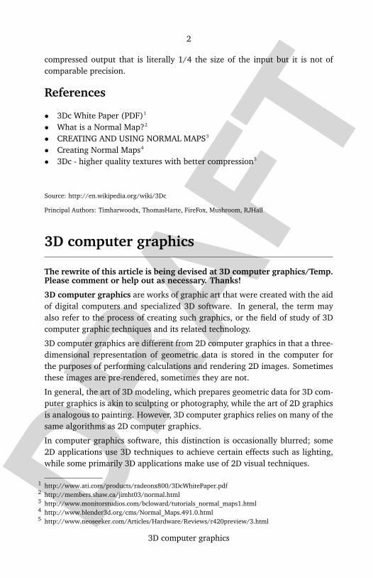
compressed output that is literally 1/4 the size of the input but it is not ofcomparable precision.

References

• 3Dc White Paper (PDF)1

• What is a Normal Map?2

• CREATING AND USING NORMAL MAPS3

• Creating Normal Maps4

• 3Dc - higher quality textures with better compression5

Source: http://en.wikipedia.org/wiki/3Dc

Principal Authors: Timharwoodx, ThomasHarte, FireFox, Mushroom, RJHall


The rewrite of this article is being devised at 3D computer graphics/Temp.Please comment or help out as necessary. Thanks!

3D computer graphics are works of graphic art that were created with the aidof digital computers and specialized 3D software. In general, the term mayalso refer to the process of creating such graphics, or the field of study of 3Dcomputer graphic techniques and its related technology.

3D computer graphics are different from 2D computer graphics in that a three-dimensional representation of geometric data is stored in the computer forthe purposes of performing calculations and rendering 2D images. Sometimesthese images are pre-rendered, sometimes they are not.

In general, the art of 3D modeling, which prepares geometric data for 3D com-puter graphics is akin to sculpting or photography, while the art of 2D graphicsis analogous to painting. However, 3D computer graphics relies on many of thesame algorithms as 2D computer graphics.

In computer graphics software, this distinction is occasionally blurred; some2D applications use 3D techniques to achieve certain effects such as lighting,while some primarily 3D applications make use of 2D visual techniques.

http://www.ati.com/products/radeonx800/3DcWhitePaper.pdf1

http://members.shaw.ca/jimht03/normal.html2

http://www.monitorstudios.com/bcloward/tutorials_normal_maps1.html3

http://www.blender3d.org/cms/Normal_Maps.491.0.html4

http://www.neoseeker.com/Articles/Hardware/Reviews/r420preview/3.html5

DRAF

T

3


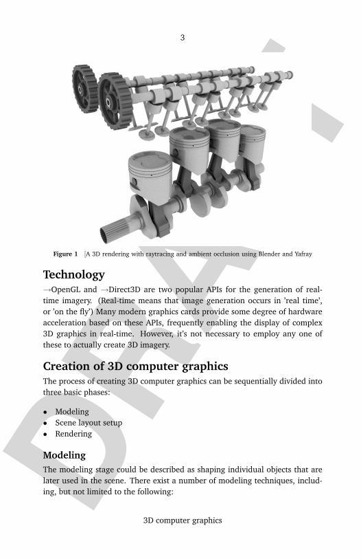
Figure 1 [A 3D rendering with raytracing and ambient occlusion using Blender and Yafray

Technology→OpenGL and →Direct3D are two popular APIs for the generation of real-time imagery. (Real-time means that image generation occurs in ’real time’,or ’on the fly’) Many modern graphics cards provide some degree of hardwareacceleration based on these APIs, frequently enabling the display of complex3D graphics in real-time. However, it’s not necessary to employ any one ofthese to actually create 3D imagery.

Creation of 3D computer graphicsThe process of creating 3D computer graphics can be sequentially divided intothree basic phases:

• Modeling• Scene layout setup• Rendering

ModelingThe modeling stage could be described as shaping individual objects that arelater used in the scene. There exist a number of modeling techniques, includ-ing, but not limited to the following:

DRAF

T

4


Figure 2 Architectural rendering compositing of modeling and lighting finalized by renderingprocess

• constructive solid geometry• NURBS modeling• polygonal modeling• subdivision surfaces• implicit surfaces

Modeling processes may also include editing object surface or material proper-ties (e.g., color, luminosity, diffuse and specular shading components — morecommonly called roughness and shininess, reflection characteristics, trans-parency or opacity, or index of refraction), adding textures, bump-maps andother features.

Modeling may also include various activities related to preparing a 3D modelfor animation (although in a complex character model this will become a stageof its own, known as rigging). Objects may be fitted with a skeleton, a centralframework of an object with the capability of affecting the shape or movementsof that object. This aids in the process of animation, in that the movement ofthe skeleton will automatically affect the corresponding portions of the model.See also →Forward kinematic animation and →Inverse kinematic animation.

DRAF

T

5


At the rigging stage, the model can also be given specific controls to makeanimation easier and more intuitive, such as facial expression controls andmouth shapes (phonemes) for lipsyncing.

Modeling can be performed by means of a dedicated program (e.g., LightwaveModeler, Rhinoceros 3D, Moray), an application component (Shaper, Lofter in3D Studio) or some scene description language (as in POV-Ray). In some cases,there is no strict distinction between these phases; in such cases modellingis just part of the scene creation process (this is the case, for example, withCaligari trueSpace).

Process

Scene layout setupScene setup involves arranging virtual objects, lights, cameras and other enti-ties on a scene which will later be used to produce a still image or an anima-tion. If used for animation, this phase usually makes use of a technique called"keyframing", which facilitates creation of complicated movement in the scene.With the aid of keyframing, instead of having to fix an object’s position, rota-tion, or scaling for each frame in an animation, one needs only to set up somekey frames between which states in every frame are interpolated.

Lighting is an important aspect of scene setup. As is the case in real-worldscene arrangement, lighting is a significant contributing factor to the resultingaesthetic and visual quality of the finished work. As such, it can be a difficultart to master. Lighting effects can contribute greatly to the mood and emotionalresponse effected by a scene, a fact which is well-known to photographers andtheatrical lighting technicians.

Tessellation and meshesThe process of transforming representations of objects, such as the middlepoint coordinate of a sphere and a point on its circumference into a polygonrepresentation of a sphere, is called tessellation. This step is used in polygon-based rendering, where objects are broken down from abstract representations("primitives") such as spheres, cones etc, to so-called meshes, which are nets ofinterconnected triangles.

Meshes of triangles (instead of e.g. squares) are popular as they have provento be easy to render using scanline rendering.

Polygon representations are not used in all rendering techniques, and in thesecases the tessellation step is not included in the transition from abstract repre-sentation to rendered scene.

DRAF

T

6


RenderingRendering is the final process of creating the actual 2D image or animationfrom the prepared scene. This can be compared to taking a photo or filmingthe scene after the setup is finished in real life.

Rendering for interactive media, such as games and simulations, is calculatedand displayed in real time, at rates of approximately 20 to 120 frames persecond. Animations for non-interactive media, such as video and film, arerendered much more slowly. Non-real time rendering enables the leveragingof limited processing power in order to obtain higher image quality. Renderingtimes for individual frames may vary from a few seconds to an hour or morefor complex scenes. Rendered frames are stored on a hard disk, then possiblytransferred to other media such as motion picture film or optical disk. Theseframes are then displayed sequentially at high frame rates, typically 24, 25, or30 frames per second, to achieve the illusion of movement.

There are two different ways this is done: →Ray tracing and GPU based real-time polygonal rendering. The goals are different:

Figure 3 An example of a ray-traced image that typically takes seconds or minutes torender. The photo-realism is apparent.

DRAF

T

7


In ray-tracing, the goal is photo-realism. Rendering often takes of the order ofseconds or sometimes even days (for a single image/frame). This is the basicmethod employed in films, digital media, artistic works, etc;

In real time rendering, the goal is to show as much information as possible asthe eye can process in a 30th of a second. The goal here is primarily speedand not photo-realism. In fact, here exploitations are made in the way the eye’perceives’ the world, and thus the final image presented is not necessarily thatof the real-world, but one which the eye can closely associate to. This is thebasic method employed in games, interactive worlds, VRML;

Photo-realistic image quality is often the desired outcome, and to this endseveral different, and often specialized, rendering methods have been de-veloped. These range from the distinctly non-realistic wireframe renderingthrough polygon-based rendering, to more advanced techniques such as: scan-line rendering, ray tracing, or radiosity.

Rendering software may simulate such visual effects as lens flares, depth offield or motion blur. These are attempts to simulate visual phenomena result-ing from the optical characteristics of cameras and of the human eye. Theseeffects can lend an element of realism to a scene, even if the effect is merely asimulated artifact of a camera.

Techniques have been developed for the purpose of simulating other naturally-occurring effects, such as the interaction of light with various forms of mat-ter. Examples of such techniques include particle systems (which can simulaterain, smoke, or fire), volumetric sampling (to simulate fog, dust and other spa-tial atmospheric effects), caustics (to simulate light focusing by uneven light-refracting surfaces, such as the light ripples seen on the bottom of a swimmingpool), and subsurface scattering (to simulate light reflecting inside the volumesof solid objects such as human skin).

The rendering process is computationally expensive, given the complex vari-ety of physical processes being simulated. Computer processing power hasincreased rapidly over the years, allowing for a progressively higher degree ofrealistic rendering. Film studios that produce computer-generated animationstypically make use of a render farm to generate images in a timely manner.However, falling hardware costs mean that it is entirely possible to create smallamounts of 3D animation on a home computer system.

Often renderers are included in 3D software packages, but there are some ren-dering systems that are used as plugins to popular 3D applications. Theserendering systems include Final-Render, Brazil r/s, V-Ray, mental ray, POV-Ray,and Pixar Renderman.

DRAF

T

8


The output of the renderer is often used as only one small part of a completedmotion-picture scene. Many layers of material may be rendered separately andintegrated into the final shot using compositing software.

Projection

Figure 4 Perspective Projection

Since the human eye sees three dimensions, the mathematical model repre-sented inside the computer must be transformed back so that the human eyecan correlate the image to a realistic one. But the fact that the display device- namely a monitor - can display only two dimensions means that this math-ematical model must be transferred to a two-dimensional image. Often thisis done using projection; mostly using perspective projection. The basic ideabehind the perspective projection, which unsurprisingly is the way the humaneye works, is that objects that are further away are smaller in relation to thosethat are closer to the eye. Thus, to collapse the third dimension onto a screen,a corresponding operation is carried out to remove it - in this case, a divisionoperation.

Orthogonal projection is used mainly in CAD or CAM applications where sci-entific modelling requires precise measurements and preservation of the thirddimension.

Reflection and shading modelsModern 3D computer graphics rely heavily on a simplified reflection modelcalled →Phong reflection model (not to be confused with →Phong shading).In refraction of light, an important concept is the refractive index. In most 3Dprogramming implementations, the term for this value is "index of refraction,"usually abbreviated "IOR."

DRAF

T

9


Figure 5 An example of cel shading in the OGRE3D engine.

Popular reflection rendering techniques in 3D computer graphics include:

• →Flat shading: A technique that shades each polygon of an object basedon the polygon’s "normal" and the position and intensity of a light source.

• →Gouraud shading: Invented by H. Gouraud in 1971, a fast and resource-conscious vertex shading technique used to simulate smoothly shaded sur-faces.

• →Texture mapping: A technique for simulating a large amount of surfacedetail by mapping images (textures) onto polygons.

• →Phong shading: Invented by Bui Tuong Phong, used to simulate specularhighlights and smooth shaded surfaces.

• →Bump mapping: Invented by Jim Blinn, a normal-perturbation techniqueused to simulate wrinkled surfaces.

• Cel shading: A technique used to imitate the look of hand-drawn animation.

DRAF

T

10


3D graphics APIs3D graphics have become so popular, particularly in computer games, that spe-cialized APIs (application programmer interfaces) have been created to easethe processes in all stages of computer graphics generation. These APIs havealso proved vital to computer graphics hardware manufacturers, as they pro-vide a way for programmers to access the hardware in an abstract way, whilestill taking advantage of the special hardware of this-or-that graphics card.

These APIs for 3D computer graphics are particularly popular:

• →OpenGL and the OpenGL Shading Language• →OpenGL ES 3D API for embedded devices• →Direct3D (a subset of DirectX)• RenderMan• RenderWare• →Glide API• TruDimension LC Glasses and 3D monitor API

There are also higher-level 3D scene-graph APIs which provide additional func-tionality on top of the lower-level rendering API. Such libraries under activedevelopment include:

• QSDK• Quesa• Java 3D• JSR 184 (M3G)• NVidia Scene Graph• OpenSceneGraph• OpenSG• OGRE• Irrlicht• Hoops3D

See also

• →3D model• 3D modeler• →3D projection• →Ambient occlusion• Anaglyph image - Anaglyphs are stereo pictures that are viewed with red-

blue glasses, that allow a 3D image to be perceived as 3D by the humaneye.

DRAF

T

11

3D computer graphics software

• Animation• Graphics• History of 3D Graphics - Major Milestones/Influential peo-

ple/Hardware+Software Develoments• List of 3D Artists• Magic Eye autostereograms• →Rendering (computer graphics)• Panda3D• Polarized glasses - Another method to view 3D images as 3D• VRML• X3D• 3d motion controller

Source: http://en.wikipedia.org/wiki/3D_computer_graphics

Principal Authors: Frecklefoot, Dormant25, Flamurai, Wapcaplet, Pavel Vozenilek, Michael Hardy,

Furrykef, Blaatkoala, Mikkalai, Blueshade


→3D computer graphics software is a program or collection of programs usedto create 3D computer-generated imagery. There are typically many stages inthe "pipeline" that studios use to create 3D objects for film and games, and thisarticle only covers some of the software used. Note that most of the 3D pack-ages have a very plugin-oriented architecture, and high-end plugins costingtens or hundreds of thousands of dollars are often used by studios. Larger stu-dios usually create enormous amounts of proprietary software to run alongsidethese programs.

If you are just getting started out in 3D, one of the major packages is usuallysufficient to begin learning. Remember that 3D animation can be very difficult,time-consuming, and unintuitive; a teacher or a book will likely be necessary.Most of the high-end packages have free versions designed for personal learn-ing.

Major PackagesMaya (Autodesk) is currently the leading animation program for cinema; near-ly every studio uses it. It is known as difficult to learn, but it is possibly themost powerful 3D package. When studios use Maya, they typically replaceparts of it with proprietary software. Studios will also render using Pixar’s

DRAF

T

12


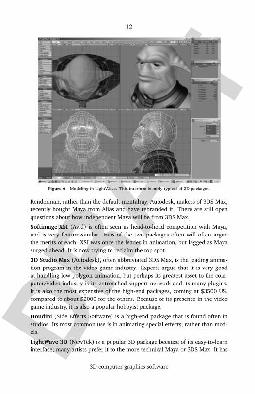
Figure 6 Modeling in LightWave. This interface is fairly typical of 3D packages.

Renderman, rather than the default mentalray. Autodesk, makers of 3DS Max,recently bought Maya from Alias and have rebranded it. There are still openquestions about how independent Maya will be from 3DS Max.

Softimage|XSI (Avid) is often seen as head-to-head competition with Maya,and is very feature-similar. Fans of the two packages often will often arguethe merits of each. XSI was once the leader in animation, but lagged as Mayasurged ahead. It is now trying to reclaim the top spot.

3D Studio Max (Autodesk), often abbreviated 3DS Max, is the leading anima-tion program in the video game industry. Experts argue that it is very goodat handling low-polygon animation, but perhaps its greatest asset to the com-puter/video industry is its entrenched support network and its many plugins.It is also the most expensive of the high-end packages, coming at $3500 US,compared to about $2000 for the others. Because of its presence in the videogame industry, it is also a popular hobbyist package.

Houdini (Side Effects Software) is a high-end package that is found often instudios. Its most common use is in animating special effects, rather than mod-els.

LightWave 3D (NewTek) is a popular 3D package because of its easy-to-learninterface; many artists prefer it to the more technical Maya or 3DS Max. It has

DRAF

T

13


weaker modeling and particularly animation features than some of the largerpackages, but it is still used widely in film and broadcasting.

Cinema 4D (MAXON) is a lighter package than the others. Its main asset isits artist-friendliness, avoiding the complicated technical nature of the otherpackages. For example, a popular plugin, BodyPaint, allows artists to drawtextures directly onto the surface of models.

formZ (autodessys, Inc.) is a general purpose 3D modeler. Its forte is mod-eling. Many of its users are architects, but also include designers from manyfields including interior designers, illustrators, product designers, set design-ers. Its default renderer uses the LightWorks rengering engine for raytracingand radiosity. formZ has been around since 1991, available for both the Mac-intosh and Windows operating systems.

Other packagesFree

Blender is a free software package that mimics the larger packages. It is beingdeveloped under the GPL, after its previous owner, Not a Number Technologies,went bankrupt. Art of Illusion is another free software package developedunder the GPL. Wings 3D is a BSD-licensed, minimal modeler. Anim8or isanother free 3d rendering and animation package.

Not Free

MilkShape 3D is a shareware/trialware polygon 3D modelling program withextensive import/export capabilities.

Carrara (Eovia) is a 3D complete tool set package for 3D modeling, texturinganimation and rendering; and Amapi and Hexagon (Eovia) are 3D packagesoften used for high-end abstract and organic modeling respectively. Bryce (DAZproductions) is most famous for landscapes. modo, created by developers whosplintered from NewTek, is a new modeling program. Zbrush(Pixologic) is adigital sculpting tool that combines 3D/2.5D modeling, texturing and painting.

RenderersPixar’s RenderMan is the premier renderer, used in many studios. Animationpackages such as 3DS Max and Maya can pipeline to RenderMan to do all therendering. mental ray is another popular renderer, and comes default withmost of the high-end packages. POV-Ray and YafRay are two free renderers.

DRAF

T

14

3D model

Related to 3D softwareSwift3D is a package for transforming models in Lightwave or 3DS Max in-to Flash animations. Match moving software is commonly used to match livevideo with computer-generated video, keeping the two in sync as the cameramoves. Poser is the most popular program for modeling people. After pro-ducing video, studios then edit or composite the video using programs such asAdobe Premiere or Apple Final Cut at the low end, or Autodesk Combustion orApple Shake at the high end.

Source: http://en.wikipedia.org/wiki/3D_computer_graphics_software

Principal Authors: Bertmg, Goncalopp, ShaunMacPherson, Snarius, Skybum

3D model

Figure 7 A 3D model of a character in the 3D modeler LightWave, shown in various manners andfrom different perspectives

A 3D model is a 3D polygonal representation of an object, usually displayedwith a computer or via some other video device. The object can range from a

DRAF

T

15

3D model

real-world entity to fictional, from atomic to huge. Anything that can exist inthe physical world can be represented as a 3D model.

3D models are most often created with special software applications called 3Dmodelers, but they need not be. Being a collection of data (points and other in-formation), 3D models can be created by hand or algorithmically. Though theymost often exist virtually (on a computer or a file on disk), even a descriptionof such a model on paper can be considered a 3D model.

3D models are widely used anywhere 3D graphics are used. Actually, theiruse predates the widespread use of 3D graphics on personal computers. Manycomputer games used pre-rendered images of 3D models as sprites before com-puters could render them in real-time.

Today, 3D models are used in a wide variety of fields. The medical industry us-es detailed models of organs. The movie industry uses them as characters andobjects for animated and real-life motion pictures. The video game industry us-es them as assets for computer and video games. The science sector uses themas highly detailed models of chemical compounds. The architecture industryuses them to demonstrate proposed buildings and landscapes. The engineer-ing community uses them as designs of new devices, vehicles and structures aswell as a host of other uses. In recent decades the earth science communityhas started to construct 3D geological models as a standard practice.

A 3D model by itself is not visual. It can be rendered as a simple wireframeat varying levels of detail, or shaded in a variety of ways. Many 3D models,however, are covered in a covering called a texture (the process of aligning thetexture to coordinates on the 3D model is called texture mapping). A textureis nothing more than a graphic image, but gives the model more detail andmakes it look more realistic. A 3D model of a person, for example, looks morerealistic with a texture of skin and clothes, than a simple monochromatic modelor wireframe of the same model.

Other effects, beyond texturing, can be done to 3D models to add to theirrealism. For example, the surface normals can be tweaked to effect how theyare lit, certain surfaces can have bump mapping applied and any other numberof 3D rendering tricks can be applied.

3D models are often animated for some uses. For example, 3D model are heav-ily animated for use in feature films and computer and video games. They canbe animated from within the 3D modeler that created them or externally. Oftenextra data is added to the model to make it easier to animate. For example,some 3D models of humans and animals have entire bone systems so they willlook realistic when they move and can be manipulated via joints and bones.

DRAF

T

16

3D projection

Source: http://en.wikipedia.org/wiki/3D_model

Principal Authors: Frecklefoot, Furrykef, HolgerK, Equendil, ZeroOne

3D projection

A 3D projection is a mathematical transformation used to project three di-mensional points onto a two dimensional plane. Often this is done to simulatethe relationship of the camera to subject. 3D projection is often the first stepin the process of representing three dimensional shapes two dimensionally incomputer graphics, a process known as rendering.

The following algorithm was a standard on early computer simulations andvideogames, and it is still in use with heavy modifications for each particularcase. This article describes the simple, general case.

Data necessary for projectionData about the objects to render is usually stored as a collection of points,linked together in triangles. Each point is a series of three numbers, represent-ing its X,Y,Z coordinates from an origin relative to the object they belong to.Each triangle is a series of three points or three indexes to points. In addition,the object has three coordinates X,Y,Z and some kind of rotation, for example,three angles alpha, beta and gamma, describing its position and orientationrelative to a "world" reference frame.

Last comes the observer (the term camera is the one commonly used). Thecamera has a second set of three X,Y,Z coordinates and three alpha, beta andgamma angles, describing the observer’s position and the direction along whichit is pointing.

All this data is usually stored in floating point, even if many programs convertit to integers at various points in the algorithm, to speed up the calculations.

• Warning: The author has used the × symbol to denote multiplication ofmatrices, e.g. ‘A×B’ to mean ‘A times B’. This is confusing since in thisfield this symbol is instead used to indicate the cross product of vectors, i.e.‘A×B’ usually means ‘A cross B’. The two operators are different. In matrixalgebra A times B is usually written as ‘A B’. I have NOT edited the rest ofthe document to reflect this.

DRAF

T

17

3D projection

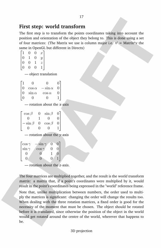
First step: world transformThe first step is to transform the points coordinates taking into account theposition and orientation of the object they belong to. This is done using a setof four matrices: (The Matrix we use is column major i.e. v’ = Matrix*v thesame in OpenGL but different in Directx)

1 0 0 x

0 1 0 y

0 0 1 z

0 0 0 1

— object translation

1 0 0 0

0 cosα − sinα 0

0 sin α cosα 0

0 0 0 1

— rotation about the x-axis

cosβ 0 sinβ 0

0 1 0 0

− sinβ 0 cosβ 0

0 0 0 1

— rotation about the y-axis

cos γ − sin γ 0 0

sin γ cos γ 0 0

0 0 1 0

0 0 0 1

— rotation about the z-axis.

The four matrices are multiplied together, and the result is the world transformmatrix: a matrix that, if a point’s coordinates were multiplied by it, wouldresult in the point’s coordinates being expressed in the "world" reference frame.

Note that, unlike multiplication between numbers, the order used to multi-ply the matrices is significant: changing the order will change the results too.When dealing with the three rotation matrices, a fixed order is good for thenecessity of the moment that must be chosen. The object should be rotatedbefore it is translated, since otherwise the position of the object in the worldwould get rotated around the centre of the world, wherever that happens tobe.

DRAF

T

18

3D projection

World transform = Translation × Rotation

To complete the transform in the most general way possible, another matrixcalled the scaling matrix is used to scale the model along the axes. This matrixis multiplied to the four given above to yield the complete world transform.The form of this matrix is:

sx 0 0 0

0 sy 0 0

0 0 sz 0

0 0 0 1

— where sx, sy, and sz are the scaling factors along the three co-ordinateaxes.

Since it is usually convenient to scale the model in its own model space or co-ordinate system, scaling should be the first transformation applied. The finaltransform thus becomes:

World transform = Translation × Rotation × Scaling

(as in some computer graphics book or some computer graphic programmingAPI such as Directx, it use mactrics with translation vectors in the bottom row,in this scheme, the order of matrices would be reversed.)

sx cos γ cosβ −sy sin γ cosβ sz sin β x

sx cos γ sin β sin α + sx sin γ cosα sy cos γ cosα − sy sin γ sin β sin α −sz cosβ sin α y

sx sin γ sinα − sx cos γ sin β cosα sy sin γ sinβ cosα + sy sin α cos γ sz cosβ cosα z

0 0 0 1

— final result of Translation × x × y × z × Scaling.

Second step: camera transformThe second step is virtually identical to the first one, except for the fact that ituses the six coordinates of the observer instead of the object, and the inversesof the matrixes should be used, and they should be multiplied in the oppo-site order. (Note that (A×B)-1=B-1×A-1.) The resulting matrix can transformcoordinates from the world reference frame to the observer’s one.

The camera looks in its z direction, the x direction is typically left, and the ydirection is typically up.

1 0 0 −x

0 1 0 −y

0 0 1 −z

0 0 0 1

DRAF

T

19

3D projection

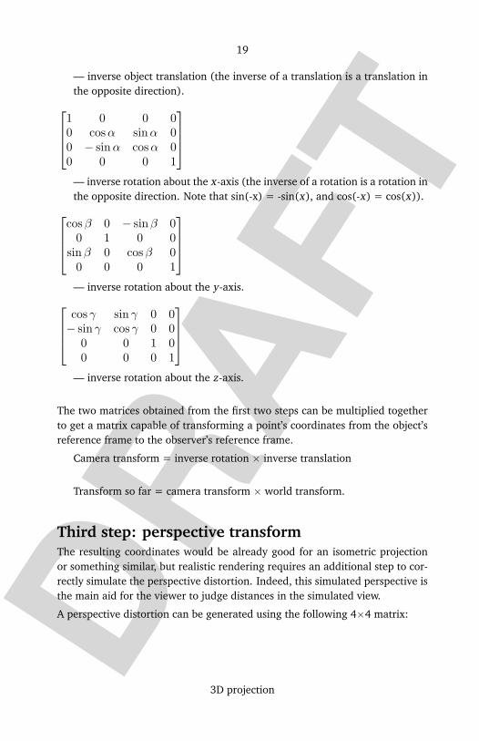
— inverse object translation (the inverse of a translation is a translation inthe opposite direction).

1 0 0 0

0 cosα sinα 0

0 − sin α cosα 0

0 0 0 1

— inverse rotation about the x-axis (the inverse of a rotation is a rotation inthe opposite direction. Note that sin(-x) = -sin(x), and cos(-x) = cos(x)).

cosβ 0 − sinβ 0

0 1 0 0

sin β 0 cosβ 0

0 0 0 1

— inverse rotation about the y-axis.

cos γ sin γ 0 0

− sinγ cos γ 0 0

0 0 1 0

0 0 0 1

— inverse rotation about the z-axis.

The two matrices obtained from the first two steps can be multiplied togetherto get a matrix capable of transforming a point’s coordinates from the object’sreference frame to the observer’s reference frame.

Camera transform = inverse rotation × inverse translation

Transform so far = camera transform × world transform.

Third step: perspective transformThe resulting coordinates would be already good for an isometric projectionor something similar, but realistic rendering requires an additional step to cor-rectly simulate the perspective distortion. Indeed, this simulated perspective isthe main aid for the viewer to judge distances in the simulated view.

A perspective distortion can be generated using the following 4×4 matrix:

DRAF

T

20

3D projection

1/ tanµ 0 0 0

0 1/ tanν 0 0

0 0B+F

B−F

−2BF

B−F

0 0 1 0

where µ is the angle between a line pointing out of the camera in z directionand the plane through the camera and the right-hand edge of the screen, andν is the angle between the same line and the plane through the camera andthe top edge of the screen. This projection should look correct, if you arelooking with one eye; your actual physical eye is located on the line through thecentre of the screen normal to the screen, and µ and ν are physically measuredassuming your eye is the camera. On typical computer screens as of 2003, tan µis probably about 11/3 times tan ν, and tan µ might be about 1 to 5, dependingon how far from the screen you are.

F is a positive number representing the distance of the observer from the frontclipping plane, which is the closest any object can be to the camera. B isa positive number representing the distance to the back clipping plane, thefarthest away any object can be. If objects can be at an unlimited distancefrom the camera, B can be infinite, in which case (B + F)/(B - F) = 1 and-2BF/(B - F) = -2F.

If you are not using a Z-buffer and all objects are in front of the camera, youcan just use 0 instead of (B + F)/(B - F) and -2BF/(B - F). (Or anything youwant.)

All the calculated matrices can be multiplied together to get a final transfor-mation matrix. One can multiply each of the points (represented as a vector ofthree coordinates) by this matrix, and directly obtain the screen coordinate atwhich the point must be drawn. The vector must be extended to four dimen-sions using homogeneous coordinates:

x′

y′

z′

ω′

=[

Perspective transform]

×

[

Camera transform]

×

[

World transform]

×

x

y

z

1

.

Note that in computer graphics libraries, such as →OpenGL, you should givethe matrices in the opposite order as they should be applied, that is, first the

DRAF

T

21

3D projection

perspective transform, then the camera transform, then the object transform, asthe graphics library applies the transformations in the opposite order than yougive the transformations in! This is useful, since the world transform typical-ly changes more often than the camera transform, and the camera transformchanges more often than the perspective transform. One can, for example,pop the world transform off a stack of transforms and multiply a new worldtransform on, without having to do anything with the camera transform andperspective transform.

Remember that x’/ω’, y’/ω’ is the final coordinates, where -1, -1 is typicallythe bottom left corner of the screen, 1, 1 is the top right corner of the screen,1, -1 is the bottom right corner of the screen and -1, 1 is the top left cornerof the screen.

If the resulting image may turn out upside down, swap the top and bottom.

If using a Z-buffer, a z’/ω’ value of -1 corresponds to the front of the Z-buffer,and a value of 1 corresponds to the back of the Z-buffer. If the front clippingplane is too close, a finite precision Z-buffer will be more inaccurate. The sameapplies to the back clipping plane, but to a significantly lesser degree; a Z-buffer works correctly with the back clipping plane at an infinite distance, butnot with the front clipping plane at 0 distance.

Objects should only be drawn where -1 ≤ z’/ω’ ≤ 1. If it is less than -1, theobject is in front of the front clipping plane. If it is more than 1, the object isbehind the back clipping plane. To draw a simple single-colour triangle, x’/ω’,y’/ω’ for the three corners contains sufficient information. To draw a texturedtriangle, where one of the corners of the triangle is behind the camera, all thecoordinates x’, y’, z’, ω’ for all three points are needed, otherwise the texturewould not have the correct perspective, and the point behind the camera wouldnot appear in the correct location. In fact, the projection of a triangle where apoint is behind the camera is not technically a triangle, since the area is infiniteand two of the angles sum to more than 180, the third angle being effectivelynegative. (Typical modern graphics libraries use all four coordinates, and cancorrectly draw "triangles" with some points behind the camera.) Also, if a pointis on the plane through the camera normal to the camera direction, ω’ is 0, andx’/ω’, y’/ω’ is meaningless.

Simple versionX2D = X3D − DX

Z3D+Eye distance ×X3D

Y2D = Y3D − DYZ3D+Eye distance × Y3D

DRAF

T

22

Ambient occlusion

where DXDY is the distance between the eye and the 3D point in the X/Y axis, a

large positive Z is towards the horizon and 0 is screen.

See also

• Computer graphics• →3D computer graphics• Graphics card• →Transform and lighting• →Texture mapping• Perspective distortion

Source: http://en.wikipedia.org/wiki/3D_projection

Principal Authors: Michael Hardy, Cyp, Alfio, Oleg Alexandrov, Bobbygao

Ambient occlusion

Ambient occlusion is a shading method used in→3D computer graphics whichhelps add realism to local reflection models by taking into account attenuationof light due to occlusion. Unlike local methods like →Phong shading, ambientocclusion is a global method, meaning the illumination at each point is a func-tion of other geometry in the scene. However, it is a very crude approximationto full global illumination. The soft appearance achieved by ambient occlusionalone is similar to the way an object appears on an overcast day.

Ambient occlusion is most often calculated by casting rays in every directionfrom the surface. Rays which reach the background or “sky” increase thebrightness of the surface, whereas a ray which hits any other object contributesno illumination. As a result, points surrounded by a large amount of geometryare rendered dark, whereas points with little geometry on the visible hemi-sphere appear light.

Ambient occlusion is related to accessibility shading, which determines appear-ance based on how easy it is for a surface to be touched by various elements(e.g., dirt, light, etc.). It has been popularized in production animation dueto its relative simplicity and efficiency. In industry, ambient occlusion is oftenreferred to as "sky light."

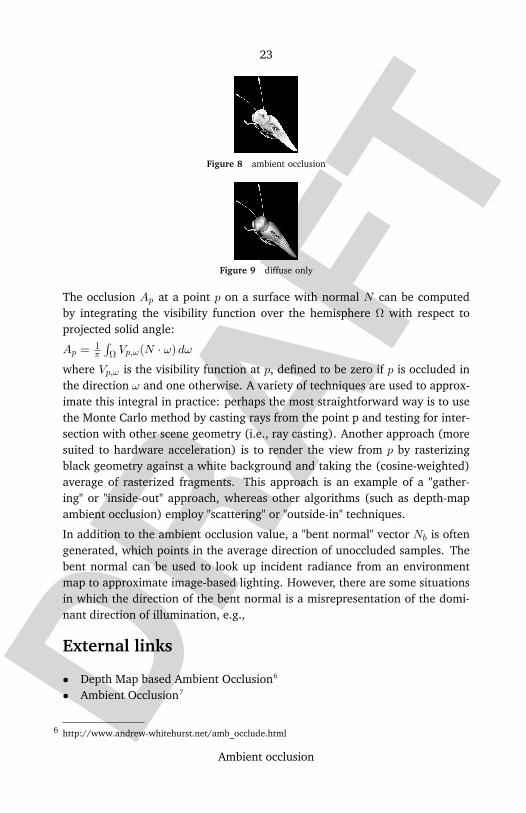
DRAF

T

23

Ambient occlusion

Figure 8 ambient occlusion

Figure 9 diffuse only

The occlusion Ap at a point p on a surface with normal N can be computedby integrating the visibility function over the hemisphere Ω with respect toprojected solid angle:

Ap = 1π

∫Ω Vp,ω(N · ω) dω

where Vp,ω is the visibility function at p, defined to be zero if p is occluded inthe direction ω and one otherwise. A variety of techniques are used to approx-imate this integral in practice: perhaps the most straightforward way is to usethe Monte Carlo method by casting rays from the point p and testing for inter-section with other scene geometry (i.e., ray casting). Another approach (moresuited to hardware acceleration) is to render the view from p by rasterizingblack geometry against a white background and taking the (cosine-weighted)average of rasterized fragments. This approach is an example of a "gather-ing" or "inside-out" approach, whereas other algorithms (such as depth-mapambient occlusion) employ "scattering" or "outside-in" techniques.

In addition to the ambient occlusion value, a "bent normal" vector Nb is oftengenerated, which points in the average direction of unoccluded samples. Thebent normal can be used to look up incident radiance from an environmentmap to approximate image-based lighting. However, there are some situationsin which the direction of the bent normal is a misrepresentation of the domi-nant direction of illumination, e.g.,

External links

• Depth Map based Ambient Occlusion6

• Ambient Occlusion7

http://www.andrew-whitehurst.net/amb_occlude.html6

DRAF

T

24

Ambient occlusion

Figure 10 combinedambient and diffuse

Figure 11 am-bient occlusion

• Assorted notes about ambient occlusion8

• Ambient Occlusion Fields9 — real-time ambient occlusion using cube maps• Fast Precomputed Ambient Occlusion for Proximity Shadows10 real-time

ambient occlusion using volume textures• Dynamic Ambient Occlusion and Indirect Lighting11 a real time self ambient

occlusion method from Nvidia’s GPU Gems 2 book• ShadeVis12 an open source tool for computing ambient occlusion

Source: http://en.wikipedia.org/wiki/Ambient_occlusion

Principal Authors: Mrtheplague, ALoopingIcon, SimonP, Gaius Cornelius, Jotapeh

http://www-viz.tamu.edu/students/bmoyer/617/ambocc/7

http://www.cs.unc.edu/~coombe/research/ao/8

http://www.tml.hut.fi/~janne/aofields/9

http://www.inria.fr/rrrt/rr-5779.html10

http://download.nvidia.com/developer/GPU_Gems_2/GPU_Gems2_ch14.pdf11

http://vcg.sourceforge.net/tiki-index.php?page=ShadeVis12

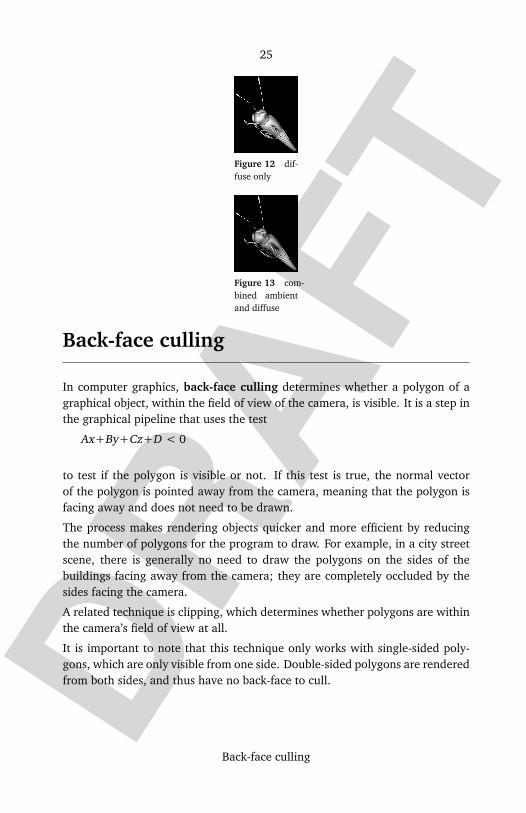
DRAF

T

25

Back-face culling

Figure 12 dif-fuse only

Figure 13 com-bined ambientand diffuse

Back-face culling

In computer graphics, back-face culling determines whether a polygon of agraphical object, within the field of view of the camera, is visible. It is a step inthe graphical pipeline that uses the test

Ax+By+Cz+D < 0

to test if the polygon is visible or not. If this test is true, the normal vectorof the polygon is pointed away from the camera, meaning that the polygon isfacing away and does not need to be drawn.

The process makes rendering objects quicker and more efficient by reducingthe number of polygons for the program to draw. For example, in a city streetscene, there is generally no need to draw the polygons on the sides of thebuildings facing away from the camera; they are completely occluded by thesides facing the camera.

A related technique is clipping, which determines whether polygons are withinthe camera’s field of view at all.

It is important to note that this technique only works with single-sided poly-gons, which are only visible from one side. Double-sided polygons are renderedfrom both sides, and thus have no back-face to cull.

DRAF

T

26

Beam tracing

Figure 14 am-bient occlusion

Figure 15 dif-fuse only

Further reading

• Geometry Culling in 3D Engines13, by Pietari Laurila

Source: http://en.wikipedia.org/wiki/Back-face_culling

Principal Authors: Eric119, Charles Matthews, Mdd4696, Deepomega, Canderson7

Beam tracing

Beam tracing is a derivative of the ray tracing algorithm that replaces rays,which have no thickness, with beams. Beams are shaped like unbounded pyra-mids, with (possibly complex) polygonal cross sections. Beam tracing was firstproposed by Paul Heckbert and Pat Hanrahan.

In beam tracing, a pyramidal beam is initially cast through the entire viewingfrustum. This initial viewing beam is intersected with each polygon in theenvironment, from nearest to farthest. Each polygon that intersects with thebeam must be visible, and is removed from the shape of the beam and added toa render queue. When a beam intersects with a reflective or refractive polygon,a new beam is created in a similar fashion to ray-tracing.

A variant of beam tracing casts a pyramidal beam through each pixel of theimage plane. This is then split up into sub-beams based on its intersection with

http://www.gamedev.net/reference/articles/article1212.asp13

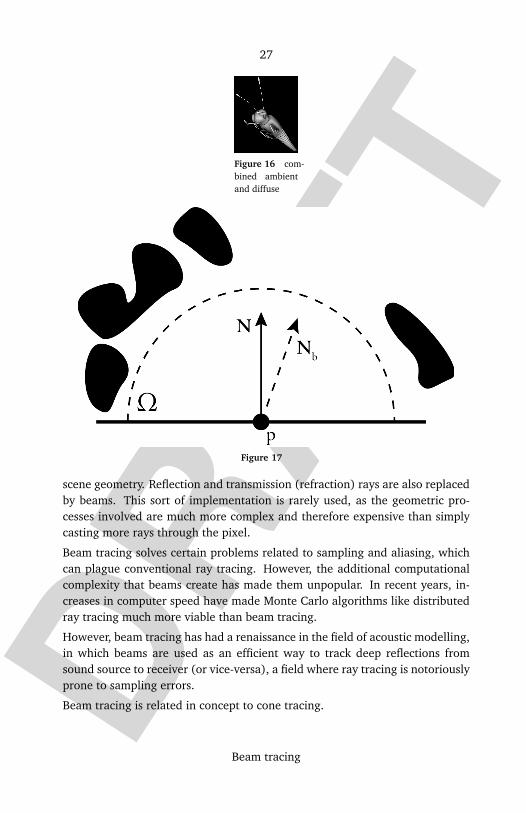
DRAF

T

27

Beam tracing

Figure 16 com-bined ambientand diffuse

Figure 17

scene geometry. Reflection and transmission (refraction) rays are also replacedby beams. This sort of implementation is rarely used, as the geometric pro-cesses involved are much more complex and therefore expensive than simplycasting more rays through the pixel.

Beam tracing solves certain problems related to sampling and aliasing, whichcan plague conventional ray tracing. However, the additional computationalcomplexity that beams create has made them unpopular. In recent years, in-creases in computer speed have made Monte Carlo algorithms like distributedray tracing much more viable than beam tracing.

However, beam tracing has had a renaissance in the field of acoustic modelling,in which beams are used as an efficient way to track deep reflections fromsound source to receiver (or vice-versa), a field where ray tracing is notoriouslyprone to sampling errors.

Beam tracing is related in concept to cone tracing.

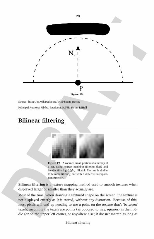
DRAF

T

28

Bilinear filtering

Figure 18

Source: http://en.wikipedia.org/wiki/Beam_tracing

Principal Authors: Kibibu, Reedbeta, RJFJR, Hetar, RJHall

Bilinear filtering

Figure 19 A zoomed small portion of a bitmap ofa cat, using nearest neighbor filtering (left) andbicubic filtering (right). Bicubic filtering is similarto bilinear filtering but with a different interpola-tion function.

Bilinear filtering is a texture mapping method used to smooth textures whendisplayed larger or smaller than they actually are.

Most of the time, when drawing a textured shape on the screen, the texture isnot displayed exactly as it is stored, without any distortion. Because of this,most pixels will end up needing to use a point on the texture that’s ’between’texels, assuming the texels are points (as opposed to, say, squares) in the mid-dle (or on the upper left corner, or anywhere else; it doesn’t matter, as long as

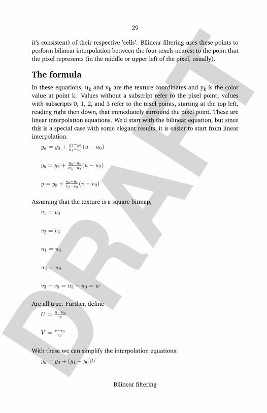
DRAF

T

29

Bilinear filtering

it’s consistent) of their respective ’cells’. Bilinear filtering uses these points toperform bilinear interpolation between the four texels nearest to the point thatthe pixel represents (in the middle or upper left of the pixel, usually).

The formulaIn these equations, uk and vk are the texture coordinates and yk is the colorvalue at point k. Values without a subscript refer to the pixel point; valueswith subscripts 0, 1, 2, and 3 refer to the texel points, starting at the top left,reading right then down, that immediately surround the pixel point. These arelinear interpolation equations. We’d start with the bilinear equation, but sincethis is a special case with some elegant results, it is easier to start from linearinterpolation.

ya = y0 + y1−y0u1−u0

(u− u0)

yb = y2 + y3−y2u3−u2

(u− u2)

y = yb + yb−yav2−v0

(v − v0)

Assuming that the texture is a square bitmap,

v1 = v0

v2 = v3

u1 = u3

u2 = u0

v3 − v0 = u3 − u0 = w

Are all true. Further, define

U = u−u0w

V = v−v0w

With these we can simplify the interpolation equations:

ya = y0 + (y1 − y0)U

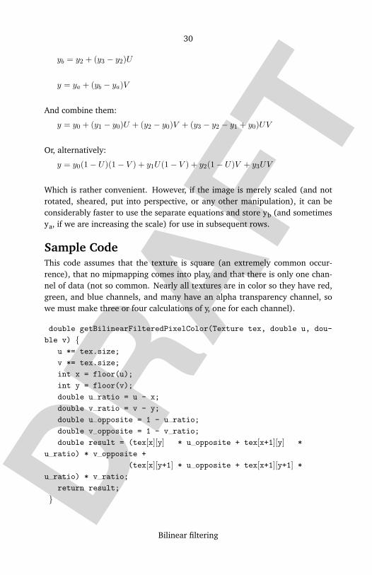
DRAF

T

30

Bilinear filtering

yb = y2 + (y3 − y2)U

y = ya + (yb − ya)V

And combine them:

y = y0 + (y1 − y0)U + (y2 − y0)V + (y3 − y2 − y1 + y0)UV

Or, alternatively:

y = y0(1− U)(1− V ) + y1U(1− V ) + y2(1− U)V + y3UV

Which is rather convenient. However, if the image is merely scaled (and notrotated, sheared, put into perspective, or any other manipulation), it can beconsiderably faster to use the separate equations and store yb (and sometimesya, if we are increasing the scale) for use in subsequent rows.

Sample CodeThis code assumes that the texture is square (an extremely common occur-rence), that no mipmapping comes into play, and that there is only one chan-nel of data (not so common. Nearly all textures are in color so they have red,green, and blue channels, and many have an alpha transparency channel, sowe must make three or four calculations of y, one for each channel).

double getBilinearFilteredPixelColor(Texture tex, double u, dou-

ble v) u *= tex.size;

v *= tex.size;

int x = floor(u);

int y = floor(v);

double u ratio = u - x;

double v ratio = v - y;

double u opposite = 1 - u ratio;

double v opposite = 1 - v ratio;

double result = (tex[x][y] * u opposite + tex[x+1][y] *

u ratio) * v opposite +

(tex[x][y+1] * u opposite + tex[x+1][y+1] *

u ratio) * v ratio;

return result;

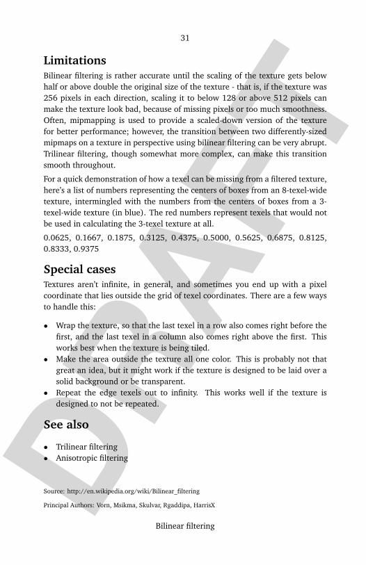
DRAF

T

31

Bilinear filtering

LimitationsBilinear filtering is rather accurate until the scaling of the texture gets belowhalf or above double the original size of the texture - that is, if the texture was256 pixels in each direction, scaling it to below 128 or above 512 pixels canmake the texture look bad, because of missing pixels or too much smoothness.Often, mipmapping is used to provide a scaled-down version of the texturefor better performance; however, the transition between two differently-sizedmipmaps on a texture in perspective using bilinear filtering can be very abrupt.Trilinear filtering, though somewhat more complex, can make this transitionsmooth throughout.

For a quick demonstration of how a texel can be missing from a filtered texture,here’s a list of numbers representing the centers of boxes from an 8-texel-widetexture, intermingled with the numbers from the centers of boxes from a 3-texel-wide texture (in blue). The red numbers represent texels that would notbe used in calculating the 3-texel texture at all.

0.0625, 0.1667, 0.1875, 0.3125, 0.4375, 0.5000, 0.5625, 0.6875, 0.8125,0.8333, 0.9375

Special casesTextures aren’t infinite, in general, and sometimes you end up with a pixelcoordinate that lies outside the grid of texel coordinates. There are a few waysto handle this:

• Wrap the texture, so that the last texel in a row also comes right before thefirst, and the last texel in a column also comes right above the first. Thisworks best when the texture is being tiled.

• Make the area outside the texture all one color. This is probably not thatgreat an idea, but it might work if the texture is designed to be laid over asolid background or be transparent.

• Repeat the edge texels out to infinity. This works well if the texture isdesigned to not be repeated.

See also

• Trilinear filtering• Anisotropic filtering

Source: http://en.wikipedia.org/wiki/Bilinear_filtering

Principal Authors: Vorn, Msikma, Skulvar, Rgaddipa, HarrisX

DRAF

T

32

Blinn–Phong shading model

Blinn–Phong shading model

The Blinn-Phong shading model (also called Blinn-Phong reflection modelor modified Phong reflection model) is a modification to the →Phong reflec-tion model, trading visual precision for computing efficiency.

In Phong shading, one must continually recalculate the angle R · V between aviewer (V) and the beam from a light-source (L) reflected (R) on a surface.

If we instead calculate a halfway vector between the viewer and light-sourcevectors,

H = L+V|L+V |

we can replace R · V with N ·H.

This dot product represents the cosine of an angle that is half of the anglerepresented by Phong’s dot product, if V, L, N and R all lie in the same plane.The angle between N and H is therefore sometimes called the halfway angle.

The halfway angle is smaller than the angle we want in Phong’s model, butconsidering that Phong is using (R · V )α, we can set an exponent α′ so that(N ·H)α′ is closer to the former expression.

Blinn-Phong is the default shading model used in →OpenGL, and is carried outon each vertex as it passes down the graphics pipeline; pixel values betweenvertices are interpolated by →Gouraud shading by default, rather than themore expensive →Phong shading.

See also

• →Phong reflection model for Phong’s corresponding model• →Phong shading• →Gouraud shading

Source: http://en.wikipedia.org/wiki/Blinn%E2%80%93Phong_shading_model

DRAF

T

33

Bloom (shader effect)

Bloom (shader effect)

Figure 20 Doom 3 mini-mod showing the bloom shader effect (screenshot by Motoxpro @doom3world )

Bloom (sometimes referred to as Light bloom) is a computer graphics shadereffect used by computer games.

In high dynamic range rendering (HDR) applications, it is used when the neces-sary brightness exceeds the contrast ratio that a computer monitor can display.A bloom works by radiating, or blooming, the high intensity light around thevery bright object, so that the bright light appears to be coming from aroundthe object, not only from the object itself. This gives the illusion that the objectis brighter than it really is. It can be used without HDR rendering to representa surface that is being illuminated with an extremely bright light source, andas a result, is often mistaken for a full implementation of HDR Rendering.

Bloom became very popular after Tron 2.0 and is used in many games andmodifications. The first game to use blooming was Deus Ex: Invisible War.

DRAF

T

34

Bounding volume

See also

• →High dynamic range rendering• Tone mapping

Source: http://en.wikipedia.org/wiki/Bloom_%28shader_effect%29

Bounding volume

Figure 21 A bounding box for a three dimensional model

In computer graphics and computational geometry, a bounding volume fora set of objects is a closed volume that completely contains the union of theobjects in the set. Bounding volumes are used to improve the efficiency of geo-metrical operations by using simple volumes to contain more complex objects.Normally, simpler volumes have simpler ways to test for overlap.

DRAF

T

35

Bounding volume

A bounding volume for a set of objects is also a bounding volume for the singleobject consisting of their union, and the other way around. Therefore it is pos-sible to confine the description to the case of a single object, which is assumedto be non-empty and bounded (finite).

Uses of bounding volumesBounding volumes are most often used to accelerate certain kinds of tests.

In ray tracing, bounding volumes are used in ray-intersection tests, and inmany rendering algorithms, it is used for viewing frustum tests. If the ray orviewing frustum does not intersect the bounding volume, it cannot intersectthe object contained in the volume. These intersection tests produce a list ofobjects that must be displayed. Here, displayed means rendered or rasterized.

In collision detection, when two bounding volumes do not intersect, then thecontained objects cannot collide, either.

Testing against a bounding volume is typically much faster than testing againstthe object itself, because of the bounding volume’s simpler geometry. This isbecause an ’object’ is typically composed of polygons or data structures thatare reduced to polygonal approximations. In either case, it is computationallywasteful to test each polygon against the view volume if the object is not visible.(Onscreen objects must be ’clipped’ to the screen, regardless of whether theirsurfaces are actually visible.)

To obtain bounding volumes of complex objects, a common way is to break theobjects/scene down using a scene graph or more specifically bounding volumehierarchies like e.g. OBB trees. The basic idea behind this is to organize a scenein a tree-like structure where the root comprises the whole scene and each leafcontains a smaller subpart.

Common types of bounding volumeThe choice of the type of bounding volume for a given application is deter-mined by a variety of factors: the computational cost of computing a boundingvolume for an object, the cost of updating it in applications in which the objectscan move or change shape or size, the cost of determining intersections, andthe desired precision of the intesection test. It is common to use several typesin conjunction, such as a cheap one for a quick but rough test in conjunctionwith a more precise but also more expensive type.

The types treated here all give convex bounding volumes. If the object beingbounded is known to be convex, this is not a restriction. If non-convex bound-ing volumes are required, an approach is to represent them as a union of a

DRAF

T

36

Bounding volume

number of convex bounding volumes. Unfortunately, intersection tests becomequickly more expensive as the bounding boxes become more sophisticated.

A bounding sphere is a sphere containing the object. In 2-D graphics, thisis a circle. Bounding spheres are represented by centre and radius. They arevery quick to test for collision with each other: two spheres intersect when thedistance between their centres does not exceed the sum of their radii. Thismakes bounding spheres appropriate for objects that can move in any numberof dimensions.

A bounding cylinder is a cylinder containing the object. In most applicationsthe axis of the cylinder is aligned with the vertical direction of the scene. Cylin-ders are appropriate for 3-D objects that can only rotate about a vertical axisbut not about other axes, and are constrained to move by horizontal transla-tion only, orthogonal to the vertical axis. Two vertical-axis-aligned cylindersintersect when, simultaneously, their projections on the vertical axis intersect –which are two line segments – as well their projections on the horizontal plane– two circular disks. Both are easy to test. In video games, bounding cylindersare often used as bounding volumes for people standing upright.

A bounding box is a cuboid, or in 2-D a rectangle, containing the object. Indynamical simulation, bounding boxes are preferred to other shapes of bound-ing volume such as bounding spheres or cylinders for objects that are roughlycuboid in shape when the intersection test needs to be fairly accurate. Thebenefit is obvious, for example, for objects that rest upon other, such as a carresting on the ground: a bounding sphere would show the car as possibly in-tersecting with the ground, which then would need to be rejected by a moreexpensive test of the actual model of the car; a bounding box immediatelyshows the car as not intersecting with the ground, saving the more expensivetest.

In many applications the bounding box is aligned with the axes of the co-ordinate system, and it is then known as an axis-aligned bounding box(AABB). To distinguish the general case from an AABB, an arbitrary boundingbox is sometimes called an oriented bounding box (OBB). AABBs are muchsimpler to test for intersection than OBBs, but have the disadvantage that theycannot be rotated.

A discrete oriented polytope (DOP) generalizes the AABB. A DOP is a convexpolytope containing the object (in 2-D a polygon; in 3-D a polyhedron), con-structed by taking a number of suitably oriented planes at infinity and movingthem until they collide with the object. The DOP is then the convex polytoperesulting from intersection of the half-spaces bounded by the planes. Popularchoices for constructing DOPs in 3-D graphics include the axis-aligned bound-ing box, made from 6 axis-aligned planes, and the beveled bounding box,

DRAF

T

37

Bounding volume

made from 10 (if beveled only on vertical edges, say) 18 (if beveled on alledges), or 26 planes (if beveled on all edges and corners). A DOP constructedfrom k planes is called a k -DOP; the actual number of faces can be less than k,since some can become degenerate, shrunk to an edge or a vertex.

A convex hull is the smallest convex volume containing the object. If the objectis the union of a finite set of points, its convex hull is a polytope, and in factthe smallest possible containing polytope.

Basic Intersection ChecksFor some types of bounding volume (OBB and Convex Polyhedra), an effectivecheck is that of the Separating Axis Test. The idea here is that, if there existsan axis by which the objects do not overlap, then the objects do not intersect.Usually the axes checked are those of the basic axes for the volumes (the unitaxes in the case of an AABB, or the 3 base axes from each OBB in the caseof OBBs). Often, this is followed by also checking the cross-products of theprevious axes (one axis from each object).

In the case of an AABB, this tests becomes a simple set of overlap tests in termsof the unit axes. For an AABB defined by M,N against one defined by O,P theydo not intersect if (Mx>Px) or (Ox>Nx) or (My>Py) or (Oy>Ny) or (Mz>Pz)or (Oz>Nz).

An AABB can also be projected along an axis, for example, if it has edges oflength L and is centered at C, and is being projected along the axis N:r=0.5Lx|Nx|+0.5Ly|Ny|+0.5Lz|Nz|, and b=C*N or b=CxNx+CyNy+CzNz, andm=b-r, n=b+rwhere m and n are the minimum and maximum extents.

An OBB is similar in this respect, but is slightly more complicated. For an OBBwith L and C as above, and with I, J, and K as the OBB’s base axes, then:r=0.5Lx|N*I|+0.5Ly|N*J|+0.5Lz|N*K|m=C*N-r and n=C*N+r

For the ranges m,n and o,p it can be said that they do not intersect if m>por o>n. Thus, by projecting the ranges of 2 OBBs along the I, J, and K axesof each OBB, and checking for non-intersection, it is possible to detect non-intersection. By additionally checking along the cross products of these axes(I0×I1, I0×J1, ...) one can be more certain that intersection is impossible.

This concept of determining non-intersection via use of axis projection alsoextends to Convex Polyhedra, however with the normals of each polyhedralface being used instead of the base axes, and with the extents being based on

DRAF

T

38

Box modeling

the minimum and maximum dot products of each vertex against the axes. Notethat this description assumes the checks are being done in world space.

External link

• Illustration of several DOPs for the same model, from epicgames.com14

Source: http://en.wikipedia.org/wiki/Bounding_volume

Principal Authors: Gdr, Lambiam, Jaredwf, Tosha, Frank Shearar

Box modeling

Box modeling is a technique in 3D modeling where the model is created bymodifying primitive shapes in a way to create a "rough draft" of the final model.This is in contrast with the edge modeling method, where the modeler edits in-dividual vertices. While a primary function of box modeling involves extrudingand scaling the flat planes that make up a model, called faces, another, moreprominent feature of this art style gives it a second, less rudimentary name ofsubdivision modeling.

SubdivisionSubdivision modeling is derived from the idea that as a work is progressed,should the artist want to make his work appear less sharp, or "blocky", eachface would be divided up into smaller, more detailed faces (usually into sets offour). However, more experienced box modelers manage to create their modelwithout subdividing the faces of the model. Basically, box modeling is brokendown into the very basic concept of polygonal management.

QuadsQuadrilateral faces, or quads, are the fundamental entity in box modeling. Ob-viously, if one were to start off from a cube, the artist would have six quad facesto work with before extrusion. While most applications for three-dimensionalart provide abilities for faces up to any size, results are often more predictableand consistent by working with quads. This is so because of the fact if youwere to draw an X connecting the corner vertices of a quad, the surface nor-mal is nearly always the same. (We say nearly under the logic that should a

http://udn.epicgames.com/Two/CollisionTutorial/kdop_sizes.jpg14

DRAF

T

39

Bui Tuong Phong

quad be something other than a perfect parallelogram, such as a rhombus, ora trapezoid, the surface normal would not be the same.)

Advantages and disadvantagesBox modeling is a modeling method that is quick and easy to learn. It is alsoappreciably faster than placing each point individually. However, it is difficultto add high amounts of detail to models created using this technique withoutpractice.

Box modeling in web designBox modeling is also a technique used in web design to lay out the variouselements of a web page before the design is implemented in HTML or XHTML.

Source: http://en.wikipedia.org/wiki/Box_modeling

Principal Authors: Greatpoo, Furrykef, Scott5114, Jonburney, Derbeth

Bui Tuong Phong

Bui Tuong Phong (1942–1975) was a Vietnamese-born computer graphics re-searcher and pioneer. His works are most often indexed under his family name,Bui Tuong (from the Vietnamese Bùi Tuòng), which comes before his givenname by Vietnamese name convention. But his inventions are rememberedunder his given name Phong.

Dr. Bui Tuong was the inventor of the →Phong reflection model and the→Phong shading interpolation method, techniques widely used in computergraphics. Bui Tuong published the description of the algorithms in his 1973PhD dissertation15 and a 1975 paper16. He received his Ph.D. from the Univer-sity of Utah in 1973.

References

Source: http://en.wikipedia.org/wiki/Bui_Tuong_Phong

Principal Authors: Dicklyon, T-tus, Hathawayc, Calvin08, Mikkalai

Bui Tuong Phong, Illumination of Computer-Generated Images, Department of Computer Science,15

University of Utah, UTEC-CSs-73-129, July 1973.Bui Tuong Phong, "Illumination for Computer Generated Images," Comm. ACM, Vol 18(6):311-317,16

June 1975.

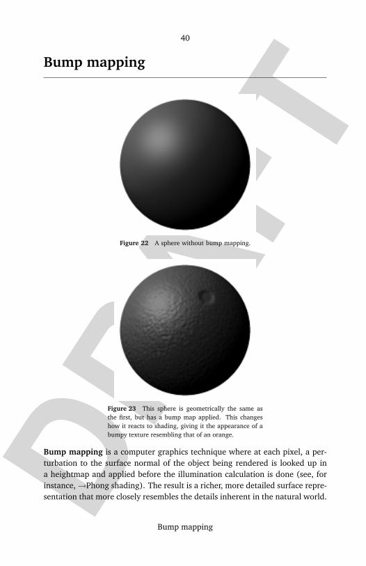
DRAF

T

40

Bump mapping

Bump mapping

Figure 22 A sphere without bump mapping.

Figure 23 This sphere is geometrically the same asthe first, but has a bump map applied. This changeshow it reacts to shading, giving it the appearance of abumpy texture resembling that of an orange.

Bump mapping is a computer graphics technique where at each pixel, a per-turbation to the surface normal of the object being rendered is looked up ina heightmap and applied before the illumination calculation is done (see, forinstance, →Phong shading). The result is a richer, more detailed surface repre-sentation that more closely resembles the details inherent in the natural world.

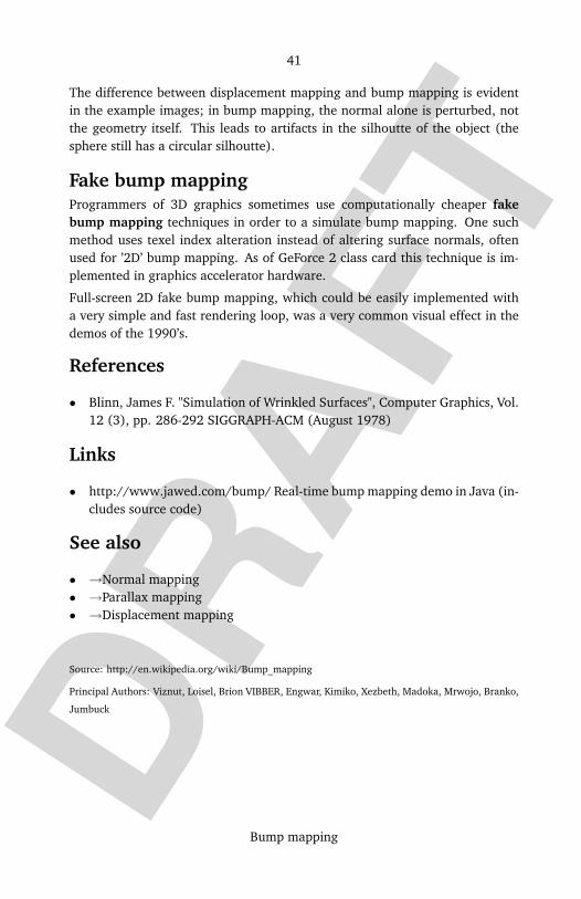
DRAF

T

41

Bump mapping

The difference between displacement mapping and bump mapping is evidentin the example images; in bump mapping, the normal alone is perturbed, notthe geometry itself. This leads to artifacts in the silhoutte of the object (thesphere still has a circular silhoutte).

Fake bump mappingProgrammers of 3D graphics sometimes use computationally cheaper fakebump mapping techniques in order to a simulate bump mapping. One suchmethod uses texel index alteration instead of altering surface normals, oftenused for ’2D’ bump mapping. As of GeForce 2 class card this technique is im-plemented in graphics accelerator hardware.

Full-screen 2D fake bump mapping, which could be easily implemented witha very simple and fast rendering loop, was a very common visual effect in thedemos of the 1990’s.

References

• Blinn, James F. "Simulation of Wrinkled Surfaces", Computer Graphics, Vol.12 (3), pp. 286-292 SIGGRAPH-ACM (August 1978)

Links

• http://www.jawed.com/bump/ Real-time bump mapping demo in Java (in-cludes source code)

See also

• →Normal mapping• →Parallax mapping• →Displacement mapping

Source: http://en.wikipedia.org/wiki/Bump_mapping

Principal Authors: Viznut, Loisel, Brion VIBBER, Engwar, Kimiko, Xezbeth, Madoka, Mrwojo, Branko,

Jumbuck

DRAF

T

42

Carmack’s Reverse

Carmack’s Reverse

Carmack’s Reverse is a →3D computer graphics technique for stencil shadowvolumes that solves the problem of when the viewer’s "eye" enters the shadowvolume by tracing backwards from some point at infinity to the eye of thecamera. It is named for one of its inventors, game programmer John Carmack.

According to a widely reported forum posting, Sim Dietrich may have pre-sented the technique to the public at a developer’s forum in 1999. WilliamBilodeau and Michael Songy filed a US patent application for the techniquethe same year. U.S. Patent 638482217 entitled "Method for rendering shadowsusing a shadow volume and a stencil buffer" issued in 2002.

Bilodeau and Songy assigned their patent ownership rights to Creative Labs.Creative Labs, in turn, granted Id Software a license to use the invention freeof charge in exchange for future support of EAX technology.

Carmack independently invented the algorithm in 2000 during the develop-ment of Doom 3. He is generally given credit for it since he, unlike Bilodeauand Songy, advertised his discovery to the larger public.

References

• Creative Pressures id Software With Patents18. Slashdot. (July 28, 2004).Retrieved on 2006-05-16.

• Creative patents Carmack’s reverse19. The Tech Report. (July 29, 2004).Retrieved on 2006-05-16.

• Creative gives background to Doom III shadow story20. The Inquirer. (July29, 2004). Retrieved on 2006-05-16.

See also

• List of software patents

Source: http://en.wikipedia.org/wiki/Carmack%27s_Reverse

Principal Authors: Frecklefoot, AlistairMcMillan, Rl, Fredrik, CesarB, Andymadigan

http://patft.uspto.gov/netacgi/nph-Parser?patentnumber=638482217

http://games.slashdot.org/games/04/07/28/1529222.shtml18

http://techreport.com/onearticle.x/711319

http://www.theinquirer.net/?article=1752520

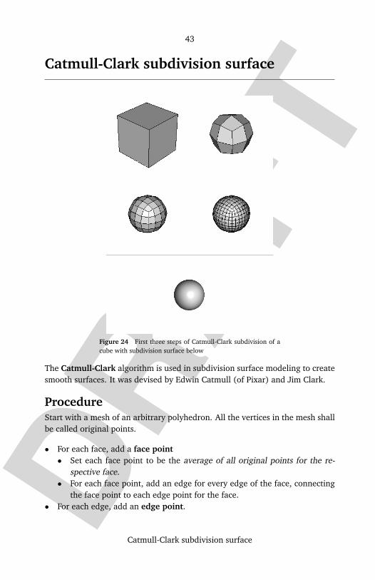
DRAF

T

43

Catmull-Clark subdivision surface


Figure 24 First three steps of Catmull-Clark subdivision of acube with subdivision surface below

The Catmull-Clark algorithm is used in subdivision surface modeling to createsmooth surfaces. It was devised by Edwin Catmull (of Pixar) and Jim Clark.

ProcedureStart with a mesh of an arbitrary polyhedron. All the vertices in the mesh shallbe called original points.

• For each face, add a face point• Set each face point to be the average of all original points for the re-

spective face.• For each face point, add an edge for every edge of the face, connecting

the face point to each edge point for the face.• For each edge, add an edge point.

DRAF

T

44


• Set each edge point to be the average of all neighbouring face pointsand original points.

• For each original point P, take the average F of all n face points for facestouching P, and take the average E of all n edge points for edges touchingP. Move each original point to the point F+2E+(n−3)P

n .

The new mesh will consist only of quadrilaterals, which won’t in general beflat. The new mesh will generally look smoother than the old mesh.

Repeated subdivision results in smoother meshes. It can be shown that thelimit surface obtained by this refinement process is at least C1

at extraordinaryvertices and C2

everywhere else.

Software using Catmull-Clark subdivision surfaces

• Art of Illusion• Blender• Wings 3D

External links

• Recursively generated B-spline surfaces on arbitrary topological surfaces21,by E. Catmull and J. Clark ( Computer-Aided Design22 10(6):350-355,November 1978).

• Catmull-Clark Subdivision Surfaces23

Source: http://en.wikipedia.org/wiki/Catmull-Clark_subdivision_surface

Principal Authors: Orderud, Ati3414, Rasmus Faber, Cyp, Mystaker1

http://www.idi.ntnu.no/~fredrior/files/Recursively%20generated%20B-spline%20surfaces%20on%20ar-21

bitrary%20topological%20surfaces.PDFhttp://www.sciencedirect.com/science/journal/0010448522

http://symbolcraft.com/graphics/subdivision/23

DRAF

T

45

Cel-shaded animation


Figure 25 Object with a basic cel-shader (AKA "toon shader") and border detection.

Cel-shaded animation (also called "cel-shading", "cell-shading", or "toonshading") is a type of non-photorealistic rendering designed to make computergraphics appear to be hand-drawn. Cel-shading is often used to mimic the styleof a comic book or cartoon. It is a quite recent addition to computer graphics,most commonly turning up in console video games. Though the end result ofcel-shading has a very simplistic feel like that of hand-drawn animation, theprocess is complex. The name comes from the clear sheets of acetate, calledcels, that are painted on for use in traditional 2D animation, such as Disneyclassics.

Process

Hand-drawn animation

Main article: Traditional animation

In hand-drawn animation or traditional animation, from the mid-19th cen-tury onwards, artists would start by creating pencil drawings; these would then

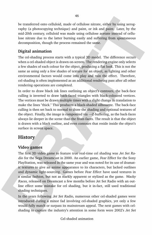
DRAF

T

46


be transferred onto celluloid, made of cellulose nitrate, either by using xerog-raphy (a photocopying technique) and paint, or ink and paint. Later, by themid-20th century, celluloid was made using cellulose acetate instead of cellu-lose nitrate due to the latter burning easily and suffering from spontaneousdecomposition, though the process remained the same.

Digital animationThe cel-shading process starts with a typical 3D model. The difference occurswhen a cel-shaded object is drawn on-screen. The rendering engine only selectsa few shades of each colour for the object, producing a flat look. This is not thesame as using only a few shades of texture for an object, as lighting and otherenvironmental factors would come into play and ruin the effect. Therefore,cel-shading is often implemented as an additional rendering pass after all otherrendering operations are completed.

In order to draw black ink lines outlining an object’s contours, the back-faceculling is inverted to draw back-faced triangles with black-coloured vertices.The vertices must be drawn multiple times with a slight change in translation tomake the lines "thick." This produces a black-shaded silhouette. The back-faceculling is then set back to normal to draw the shading and optional textures ofthe object. Finally, the image is composited via →Z-buffering, as the back-facesalways lie deeper in the scene than the front-faces. The result is that the objectis drawn with a black outline, and even contours that reside inside the object’ssurface in screen space.

History

Video gamesThe first 3D video game to feature true real-time cel shading was Jet Set Ra-dio for the Sega Dreamcast in 2000. An earlier game, Fear Effect for the SonyPlayStation, was released in the same year and was noted for its use of dramat-ic textures to give an anime appearance to its characters, but lacked outlinesand dynamic light-sourcing. Games before Fear Effect have used textures ina similar fashion, but not as starkly apparent or stylized as the game. WackyRaces, released on Dreamcast a few months before Jet Set Radio with an out-line effect some mistake for cel shading, but it in-fact, still used traditionalshading techniques.

In the years following Jet Set Radio, numerous other cel-shaded games wereintroduced during a minor fad involving cel-shaded graphics, yet only a fewwould fully match or surpass its mainstream appeal. The next games with cel-shading to capture the industry’s attention in some form were 2002’s Jet Set

DRAF

T

47


Figure 26 The Legend of Zelda: The Wind Waker is a well-known cel-shaded game

Radio Future and Sly Cooper and the Thievius Raccoonus. Over time, morecel-shaded titles such as Dark Cloud 2, Cel Damage, Klonoa 2, the Viewti-ful Joe series, and XIII were released with positive feedback, though nonewere considered blockbusters in terms of sales figures. Originally the only cel-shaded games to receive both positive ratings and sales after Sly Cooper andthe Thievius Raccoonus were The Legend of Zelda: The Wind Waker and Sly2: Band of Thieves.

NOTE: Some dispute whether games like Klonoa 2 and Sly Cooper are cel-shaded. Like Wacky Races, they use the black outline effects associated withcel-shading, but they feature smoothly shaded surfaces with gentle lightinggradiants as opposed to the harsh contrasts associated with the cel-shadingtechnique

Originally, Sega’s The House of the Dead 3 for the Xbox was cel-shaded. Ear-ly in HotD3’s development Sega released screenshots of the then current cel-shaded graphics to the gaming community. Shorty after those initial screen-shots were released, Sega announced that they were dropping the cel-shadedgraphics in favour of conventional graphic techniques. There are several sus-pected reasons for Sega’s change of heart, the most popular and most likelyis that the screenshots met much negative response from gamers who dislikedthe cel-shaded graphical style. Many gamers claimed the cel-shading was used

DRAF

T

48


purely as a gimmick in an attempt to sell more games. HotD3 was a bloody,gory and very violent light gun game which featured zombies and other mutat-ed and deformed creatures. Many felt the cel-shaded look clashed greatly withthe game’s themes and content.

The use of cel-shading in video games has slowed somewhat since its inception,but the technique continues to be employed in the modern era. Recent andupcoming examples include Dragon Quest VIII, Killer 7, Metal Gear Acid 2,and Okami.

Examples of digital cel-shadingMain article: List of cel-shaded video games

Some of the more prominent films that have featured cel-shaded graphics are:

• Appleseed• The Animatrix short films• Beyblade: The Movie - Fierce Battle• Various sequences from Futurama, a US TV series• Parts of Ghost in the Shell: Stand Alone Complex, a Japanese TV series

• The Tachikoma Days sequences at the end of the episodes are entirelyCG using cel-shading.

• Ghost in the Shell: S.A.C. 2nd GIG and Innocence: Ghost in the Shell• Hot Wheels Highway 35 World Race• Lego Exo-Force• Rescue Heroes: The Movie• Various sequences from Sonic X, a Japanese TV series• Star Wars: Clone Wars• Stuart Little 3: Call of the Wild• The Iron Giant• Tom and Jerry Blast Off to Mars

Some of the more prominent games that have featured cel-shaded graphicsare:

• Auto Modellista• Bomberman Generation• Bomberman Jetters• Cel Damage• Crazyracing Kartrider• Dark Cloud 2• Dragon Ball Z: Budokai 2, 3, and Tenkaichi

DRAF

T

49


• Dragon Quest VIII• Gungrave series• Harvest Moon: Save the Homeland• Jet Set Radio series• Killer 7• Klonoa 2• The Legend of Zelda: Phantom Hourglass• The Legend of Zelda: The Wind Waker• Mega Man X7• Mega Man X Command Mission• Metal Gear Acid 2• Monster Rancher 3• Robotech: Battlecry• Runaway: A Road Adventure• Shin Megami Tensei III: Nocturne• Shin Megami Tensei: Digital Devil Saga and Digital Devil Saga 2• Sly Cooper series• Ultimate Spider-Man• Tales of Symphonia• Tony Hawk’s American Sk8land• Viewtiful Joe series• Wild Arms 3• XIII• X-Men Legends II: Rise of Apocalypse• Zone of the Enders: The 2nd Runner

In addition, some TV series and commercials also use cel-shading effects:

• Atomic Betty• Canada’s Worst Driver• Class of the Titans• Daily Planet (2005-2006 season)• Delilah and Julius• D.I.C.E.• Dragon Booster• Duck Dodgers• Family Guy• Fairly OddParents• Funky Cops• Futurama (mainly in scene-setting shots)• G.I. Joe: Sigma 6• Gundam Seed

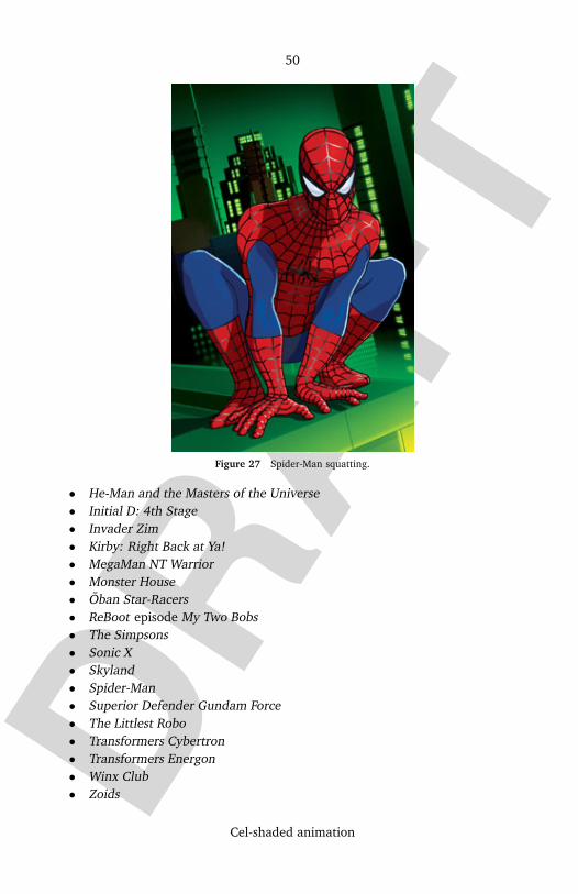
DRAF

T

50


Figure 27 Spider-Man squatting.

• He-Man and the Masters of the Universe• Initial D: 4th Stage• Invader Zim• Kirby: Right Back at Ya!• MegaMan NT Warrior• Monster House• Oban Star-Racers• ReBoot episode My Two Bobs• The Simpsons• Sonic X• Skyland• Spider-Man• Superior Defender Gundam Force• The Littlest Robo• Transformers Cybertron• Transformers Energon• Winx Club• Zoids

DRAF

T

51


• Lego Exo-Force (commercial)• McCain’s Zwak Punch (commercial)• Sola/Nero/Vena/Olera/Zonte sparking wine (commercial)

See also

• List of cel-shaded video games

Other types of animation

• Traditional animation• Special effects animation• Character animation• Computer animation and →3D computer graphics• Skeletal animation• See Animation#Styles and techniques of animation for more info

References

• CelShading.com24. More information on 3D cel-shading including an imagegallery.

• Celshader.com FAQ25. Retrieved August 2, 2005.• IGN: Jet Grind Radio Review26. Retrieved August 4, 2005.• GameDev.net - Cel-Shading27. Retrieved August 5, 2005.

Source: http://en.wikipedia.org/wiki/Cel-shaded_animation

Principal Authors: Joshfist, Jacob Poon, Andrevan, GrumpyTroll, Jacoplane, CyberSkull, MIT Trekkie,

Sherool

http://www.celshading.com/24

http://www.celshader.com/FAQ.html25

http://dreamcast.ign.com/articles/163/163512p1.html26


DRAF

T

52

Cg programming language


Cg or C for Graphics is a High level shader language created by NVIDIA forprogramming vertex and pixel shaders.

Cg is based on the C programming language and although they share the samesyntax, some features of C were modified and new data types were added tomake Cg more suitable for programming graphics processing units.

BackgroundAs a result of technical advancements in graphics cards, some areas of 3Dgraphics programming have become quite complex. To simplify the process,new features were added to graphics cards, including the ability to modifytheir rendering pipelines using vertex and pixel shaders.

In the beginning, vertex and pixel shaders were programmed at a very low levelwith only the assembly language of the graphics processing unit. Althoughusing the assembly language gave the programmer complete control over codeand flexibility, it was fairly hard to use. A portable, higher level languagefor programming the GPU was needed, so Cg was created to overcome theseproblems and make shader development easier.

Some of the benefits of using Cg over assembly are:

• High level code is easier to learn, program, read, and understand than as-sembly code.

• Cg code is portable to a wide range of hardware and platforms, unlikeassembly code, which usually depends on hardware and the platforms it’swritten for.

• The Cg compiler can optimize code and do lower level tasks automatically,which are hard to do and error prone in assembly.

Details

Data typesCg has six basic data types, some of them are the same as in C, others areespecially added for GPU programming, these types are:

• float - a 32bit floating point number• half - a 16bit floating point number• int - a 32bit integer• fixed - a 12bit fixed point number

DRAF

T

53


• bool - a boolean variable• sampler* - represents a texture object

Cg also features vector and matrix data types that are based on the basic datatypes, such as float3, float4x4, such data types are quite common when dealingwith 3D graphics programming, Cg also has struct and array data types, whichwork in a similar way to C equivalents.

OperatorsCg supports a wide range of operators, including the common arithmetic op-erators from C, the equivalent arithmetic operators for vector and matrix datatypes, and the common logical operators.

Functions and control structuresCg shares the basic control structures with C, like if/else, while, and for. It alsohas a similar way of defining functions.

The standard Cg libraryAs in C, Cg features a set of functions for common tasks in GPU programming.Some of the functions have equivalents in C, like the mathematical functionsabs and sin, while others are specialized in GPU programming tasks, like thetexture mapping functions tex1D and tex2D.

The Cg runtime libraryCg programs are merely vertex and pixel shaders, and they need supportingprograms that handle the rest of the rendering process, Cg can be used withtwo APIs, →OpenGL or DirectX, each has its own set of Cg functions to com-municate with the Cg program, like setting the current Cg shader, passing pa-rameters, and such tasks.

A sample Cg vertex shader

// input vertex

struct VertIn float4 pos : POSITION;

float4 color : COLOR0;

;

// output vertex

struct VertOut float4 pos : POSITION;

float4 color : COLOR0;

DRAF

T

54


;

// vertex shader main entry

VertOut main(VertIn IN, uniform float4x4 modelViewProj) VertOut OUT;

OUT.pos = mul(modelViewProj, IN.pos); // calculate out-

put coords

OUT.color = IN.color; // copy input color to output

OUT.color.z = 1.0f; // blue component of color = 1.0f

return OUT;

Applications and games that use Cg

• Far Cry• PlayStation 3 compatibility• Crystal Space• OGRE• Virtools Dev

Further reading

• Randima Fernando, Mark J. Kilgard, The Cg Tutorial: The Definitive Guideto Programmable Real-Time Graphics, Addison-Wesley Professional, ISBN0-32119-496-9

• Randima Fernando, GPU Gems: Programming Techniques, Tips, and Tricksfor Real-Time Graphics, Addison-Wesley Professional, ISBN 0-32122-832-4

• William R. Mark, R. Steven Glanville, Kurt Akeley, Mark J. Kilgard, Cg: ASystem for Programming Graphics Hardware in a C-like Language 28, Pro-ceedings of SIGGRAPH 200329.

• Mark J. Kilgard, Cg in Two Pages 30, 2003.

See also

• Computer programming• Computer graphics• Vertex and pixel shaders• High level shader language

http://www.cs.utexas.edu/~billmark/papers/Cg/28

http://www.cs.brown.edu/~tor/sig2003.html29

http://xxx.lanl.gov/ftp/cs/papers/0302/0302013.pdf30

DRAF

T

55


• OpenGL shading language• Shader Model• →OpenGL• DirectX

External links

• Cg in Two Pages31

• NVIDIA32

• Cg home page33

• OpenGL home page34

• DirectX home page35

• CgShaders.org36

• NeHe Cg vertex shader tutorial37

• Far Cry38

• A glimpse at Cg Shader Toolkit39

• Virtools40

Source: http://en.wikipedia.org/wiki/Cg_programming_language

Principal Authors: Ayman, Optim, Orderud, T-tus, RJHall

http://xxx.lanl.gov/ftp/cs/papers/0302/0302013.pdf31

http://www.nvidia.com/32

http://developer.nvidia.com/page/cg_main.html33

http://www.opengl.org34

http://www.microsoft.com/windows/directx/default.aspx35

http://www.cgshaders.org/36

http://nehe.gamedev.net/data/lessons/lesson.asp?lesson=4737

http://www.farcry-thegame.com/38

http://deathfall.com/feature.php?op=showcontent&id=1239

http://www.virtools.com40

DRAF

T

56

COLLADA

Clipmap

Clipmapping is a method of clipping a mipmap to a subset of data pertinentto the geometry being displayed. This is useful for loading as little data aspossible when memory is limited, such as on a graphics card.

External Links

• SGI paper from 200241

• SGI paper from 199642

• Description from SGI’s developer library43

Source: http://en.wikipedia.org/wiki/Clipmap

COLLADA

COLLADA is a COLLAborative Design Activity for establishing an interchangefile format for interactive 3D applications.

COLLADA defines a standard XML schema for data interchange.

Originally established by Sony Computer Entertainment as the official formatfor PlayStation 3 and PlayStation Portable development, COLLADA continuesto evolve through the efforts of the Khronos contributors. Dozens of commer-cial game studios and game engines have adopted the standard.

COLLADA version 1.4, released in January 2006, supports features such ascharacter skinning and morph targets, rigid body dynamics and shader effectsfor multiple shading languages including the →Cg programming language,GLSL and HLSL.

Solutions exist to transport data from one Digital Content Creation (DCC) toolto another. Supported DCCs include Maya (using ColladaMaya), 3D StudioMax (using ColladaMax), Softimage XSI and Blender. Game engines, such asUnreal engine and the open-source C4 Engine, have also adopted this format.

http://www.cs.virginia.edu/~gfx/Courses/2002/BigData/papers/Texturing/Clipmap.pdf41

http://www.sgi.com/products/software/performer/presentations/clipmap_intro.pdf42

http://techpubs.sgi.com/library/tpl/cgi-bin/getdoc.cgi?coll=0650&db=bks&srch=&fname=/SGI_De-43

veloper/Perf_PG/sgi_html/ch15.html

DRAF

T

57

COLLADA

Google Earth (release 4) has adopted COLLADA (1.4) as their native formatfor describing the objects populating the earth. Users can simply drag anddrop a COLLADA (.dae) file on top of the virtual earth. Alternatively, Googlesketchup can also be used to create .kmz files, a zip file containing a KML file,a COLLADA (.dae) file, and all the texture images.

Two open-source utility libraries are available to simplify the import and ex-port of COLLADA documents: the COLLADA DOM and the FCollada library.The COLLADA DOM is generated at compile-time from the COLLADA schema.It provides a low-level interface that eliminates the need for hand-written pars-ing routines, but is limited to reading and writing only one version of COLLA-DA, making it difficult to upgrade as new versions are released. In contrast,Feeling Software’s FCollada provides a higher-level interface and can importall versions of COLLADA. FCollada is used in ColladaMaya, ColladaMax andseveral commercial game engines.

See also

• X3D• List of vector graphics markup languages

External links

• Official homepage44

• Forum45

• COLLADA book46

• COLLADA tools including: ColladaMaya, ColladaMax, FCollada and theFeeling Viewer47

• COLLADA DOM, COLLADA RT, and COLLADA FX libraries are onsourceforge48

• Bullet Physics Library - First open source rigid body dynamics simulatorwith COLLADA Physics import49

Source: http://en.wikipedia.org/wiki/COLLADA

Principal Authors: Racklever, Karada, Agentsoo, Who, Khalid hassani, N00body

http://www.khronos.org/collada/44

http://collada.org/45

http://www.akpeters.com/product.asp?ProdCode=287646

http://www.feelingsoftware.com47

http://sourceforge.net/projects/collada-dom48

http://bullet.sourceforge.net49

DRAF

T

58

Comparison of Direct3D and OpenGL


In computer software, →Direct3D is a proprietary API designed by MicrosoftCorporation that provides a standardized API for hardware 3D acceleration onthe Windows platform. Direct3D is implemented, like OpenGL on the sameplatform, in the display driver.

→OpenGL is an open standard Application Programming Interface that pro-vides a number of functions for the rendering of 2D and 3D graphics. Animplementation is available on most modern operating systems.

Following is a comparison of the two APIs, structured around various consid-erations mostly relevant to game development.

PortabilityFor the most part, Direct3D is only implemented on Microsoft’s Windows familyof operating systems, including the embedded versions used in the Xbox familyof video game consoles. Several partially functional ports of the Direct3D APIhave been implemented by Wine, a project to port common Windows APIs toLinux, but this work is difficult due to the dependency of DirectX as a wholeon many other components of the Windows operating systems. Microsoft oncestarted development on a port to Apple Computer’s Mac OS, but later aban-doned this project.

OpenGL, on the other hand, has implementations available across a wide va-riety of platforms including Microsoft Windows, Linux, UNIX-based systems,Mac OS X and game consoles by Nintendo and Sony, such as the PlayStation 3and Wii. With the exception of Windows, all operating systems that allow forhardware-accelerated 3D graphics have chosen OpenGL as the primary API.Even more operating systems have OpenGL software renderers.

Microsoft’s supplied OpenGL driver in Windows (including Vista) provides nohardware acceleration or direct support for extensions. Microsoft’s stance onthis is that eliminating OpenGL inconveniences few and allows them to supportmore hardware in the same testing time. Other platforms supply very fewdrivers for any hardware, OpenGL or otherwise.

Windows thus requires the correct drivers from the GPU’s manufacturer orvendor for OpenGL hardware support, as well as the full performance inits Direct3D support. These manufacturer-supplied drivers nearly all includeOpenGL support through the ICD (Installable Client Driver).

In terms of portability, Direct3D is a much more limiting choice; however, this"lock-in" will only be a problem for some applications. Those aiming at the

DRAF

T

59


desktop computer gaming market should consider that its non-Windows seg-ment is still relatively small. On the other hand, while Microsoft’s segment ofthe console market is growing, it is very small, especially compared to that ofSony’s, and predicted by analysts to remain so. While no current or upcom-ing console uses exactly standard graphics APIs, the Microsoft Xbox 360 usesa variant of Direct3D while the Sony PlayStation 3 uses a variant of →OpenGLES.

Ease of useIn its earliest incarnation, Direct3D was known to be rather clumsy to use— to perform a state change, for instance, it required a number of complexoperations. For example, to enable alpha blending, one had to create a so-called execute buffer, lock it, fill it with the correct opcodes (along with astructure header telling how many opcodes the buffer contained and a special"exit" opcode), unlock it, and finally send it to the driver for execution. Incontrast, OpenGL only requires a single "glEnable(GL_BLEND);" call. The Di-rect3D model frustrated many programmers. The most famous complaint wasprobably made by high-profile game developer John Carmack in the .plan filein which he urged Microsoft to abandon Direct3D in favor of OpenGL.

Version 5 (the second version, but it was released with DirectX 5) abandonedexecute buffers and improved the API significantly, but it was still cumbersomeand didn’t provide much in terms of texture management or vertex array man-agement. Direct3D 7 provided texture management, and Direct3D 8, amongother things, provided vertex array management. Currently, Direct3D’s APIis a well-designed API. Direct3D and OpenGL still follow different paradigms,though.

Direct3D is built upon Microsoft’s COM. The use of this framework means thatC++ code is a little unusual. Functions for acquiring values don’t return thevalue in the return argument for the function because all COM functions returnan "HRESULT" that tells whether the function executed correctly or not. Theplus side of using COM is that you can use the same API in any COM-awarelanguage. These include Visual Basic and Visual Basic Script, among others.

OpenGL is a specification based on the C programming language. It is builtaround the concept of a finite state machine, though more recent OpenGL ver-sions have transformed it into much more of an object based system. Thoughthe specification is built on C, it can be implemented in other languages as well.

In general, Direct3D is designed to be a 3D hardware interface. The featuresetof D3D is derived from the featureset of what hardware provides. OpenGL, onthe other hand, is designed to be a 3D rendering system that may be hardware

DRAF

T

60


accelerated. As such, its featureset is derived from that which users find use-ful. These two API’s are fundamentally designed under two separate modes ofthought. The fact that the two APIs have become so similar in functionalityshows how well hardware is converging into user functionality.

Even so, there are functional differences in how the two APIs work. Direct3Dexpects the application to manage hardware resources; OpenGL makes theimplementation do it. This makes it much easier for the user in terms of writinga valid application, but it leaves the user more succeptible to implementationbugs that the user may be unable to fix. At the same time, because OpenGLhides hardware details (including whether hardware is even being used), theuser is unable to query the status of various hardware resources. So the usermust trust that the implementation is using hardware resources "best".

Until recently, another functional difference between the APIs was the waythey handled rendering to textures: the Direct3D method (SetRenderTarget())is convenient, while previous versions of OpenGL required the manipulation ofP-buffers (pixel buffers). This was cumbersome and risky: if the programmer’scodepath was different from that anticipated by the driver manufacturer, thecode would have fallen back to software rendering, causing a substantial per-formance drop. According to a Gamasutra article50 (registration required), theaforementioned John Carmack considered switching from OpenGL to Direct3Dbecause of the contrived use of P-buffers. However, widespread support for the"frame buffer objects" extension, which provides an OpenGL equivalent of theDirect3D method, has successfully addressed this shortcoming.

Outside of a few minor functional differences, typically with regard to render-ing to textures (the "framebuffer objects" extension did not cover everything,but the ARB is working to address this), the two APIs provide nearly the samelevel of functionality.

PerformanceShortly after the establishment of both Direct3D and OpenGL as viable graph-ics libraries, Microsoft and SGI engaged in what has been called the "API Wars".Much of the argument revolved around which API offered superior perfor-mance. This question was relevant due to the very high cost of graphics accel-erators during this time, which meant the consumer market was using softwarerenderers implemented by Microsoft for both Direct3D and OpenGL.

Microsoft had marketed Direct3D as faster based on in-house performancecomparisons of these two software libraries. The performance deficit wasblamed on the rigorous specification and conformance required of OpenGL.

http://www.gamasutra.com/features/20040830/mcguire_02.shtml50

DRAF

T

61


This perception was changed at the 1996 SIGGRAPH (Special Interest Groupon Computer Graphics) conference. At that time, SGI challenged Microsoftwith their own optimized Windows software implementation of OpenGL calledCosmoGL which in various demos matched or exceeded the performance of Di-rect3D. For SGI, this was a critical milestone as it showed that OpenGL’s poorsoftware rendering performance was due to Microsoft’s inferior implementa-tion, and not to design flaws in OpenGL itself.

Direct3D 9 and below have a particular disadvantage with regard to perfor-mance. Drawing a vertex array in Direct3D requires that the CPU switch tokernel-mode and call the graphics driver immediately. In OpenGL, because anOpenGL driver has portions that run in user-mode, can perform marshallingactivities to limit the number of kernel-mode switches and batch numerouscalls in one kernel-mode switch. In effect, the number of vertex array drawingcalls in a D3D application is limitted to the speed of the CPU, as switching tokernel-mode is a fairly slow and CPU intensive operation.

Direct3D 10 allows portions of drivers to run in user-mode, thus allowingD3D10 applications to overcome this performance limitation.

Outside of this, Direct3D and OpenGL applications have no significant perfor-mance differences.

StructureOpenGL, originally designed for then-powerful SGI workstations, includes anumber of features that are only useful for workstation applications. The APIas a whole contains about 250 calls, but only a subset of perhaps 100 are usefulfor game development. However, no official gaming-specific subset was everdefined. MiniGL, released by 3Dfx as a stopgap measure to support glQuake,might have served as a starting point, but additional features like stencil weresoon adopted by games, and support for the entire OpenGL standard contin-ued. Today, workstations and consumer machines use the same architecturesand operating systems, and so modern incarnations of the OpenGL standardstill include these features, although only special workstation-class video cardsaccelerate them.

OpenGL is designed as a feature rich API regardless of hardware support.The specification often drives the implementation of hardware acceleration forthese features. For example, when the GeForce 256 graphics card came out in1999, games like Quake III Arena could already benefit from its accelerationof Transform & Lighting, because the API was designed to provide this feature.Meanwhile, Direct3D developers had to wait for the next version of Direct3Dto be released and rewrite their games to use the new API before they couldtake advantage of hardware-based Transform and Lighting.

DRAF

T

62


The advantage of OpenGL’s inclusive, extensible approach is limited in practice,however, by the market dominance Direct3D has achieved. In recent years,games have rarely implemented features until Direct3D has supported them,and graphics cards vendors have been reluctant to implement features thatcurrent or upcoming versions of Direct3D will not support.

ExtensionsThe OpenGL extension mechanism is probably the most heavily disputed dif-ference between the two APIs. OpenGL includes a mechanism where any drivercan advertise its own extensions to the API, thus introducing new functionalitysuch as blend modes, new ways of transferring data to the GPU, or differenttexture wrapping parameters. This allows new functionality to be exposedquickly, but can lead to confusion if different vendors implement similar exten-sions with different APIs. Many of these extensions are periodically standard-ized by the OpenGL Architecture Review Board, and some are made a core partof future OpenGL revisions.

On the other hand, Direct3D is specified by one vendor (Microsoft) only, lead-ing to a more consistent API, but denying access to vendor-specific features.nVidia’s UltraShadow51 technology, for instance, is not available in the stockDirect3D APIs at the time of writing. It should be noted that Direct3D doessupport texture format extensions (via so-called FourCC’s). These were oncelittle-known and rarely used, but are now used for DXT texture compression.

When graphics cards added support for pixel shaders (known on OpenGL as"fragment programs"), Direct3D provided a single "Pixel Shader 1.1" (PS1.1)standard which the GeForce 3 and up, and Radeon 8500 and up, claimed com-patibility with. Under OpenGL the same functionality was accessed through avariety of custom extensions.

In theory, the Microsoft approach allows a single code path to support bothbrands of card, whereas under OpenGL the programmer had to write two sep-arate systems. In reality, though, because of the limits on pixel processing ofthose early cards, Pixel Shader 1.1 was nothing more than a pseudo-assemblylanguage version of the nVidia-specific OpenGL extensions. For the most part,the only cards that claimed PS 1.1 functionality were nVidia cards, and that isbecause they were built for it natively. When the Radeon 8500 was released,Microsoft released an update to Direct3D that included Pixel Shader 1.4, whichwas nothing more than a pseudo-assembly language version of the ATi-specificOpenGL extensions. The only cards that claimed PS 1.4 support were ATi cardsbecause they were designed with the precise hardware necessary to make that

http://www.nvidia.com/object/feature_ultrashadow.html51

DRAF

T

63


functionality happen. In terms of early Pixel shaders, D3D’s attempt at a singlecode path fared no better than the OpenGL mechanism.

Fortunately, this situation only existed for a short time under both APIs.Second-generation pixel shading cards were much more similar in function-ality, with each architecture evolving towards the same kind of pixel pro-cessing conclusion. As such, Pixel Shader 2.0 allowed a unified code pathunder Direct3D. Around the same time OpenGL introduced its own ARB-approved vertex and pixel shader extensions (GL_ARB_vertex_program andGL_ARB_fragment_program), and both sets of cards supported this standardas well.

The Windows Vista IssueAn issue has arisen between Direct3D and OpenGL recently (mid-to-late 2005),with regard to support for Microsoft’s new operating system, Windows Vista.The Vista OS has a feature called Desktop Compositing (which is similar inconcept to Mac OS X’s Quartz Compositor or Compiz on Linux based systems)that allows individual windows to blend into the windows beneath them aswell as a number of other cross-window effects. The new OS’s rendering systemthat allows this to function operates entirely through Direct3D; as such, everyWindows application is automatically a Direct3D application.

The ICD driver model used in prior versions of Windows will still functionhowever. There is one important caveat: activating an ICD will cause Vista todeactivate Desktop Compositing.

Note that this functionality only truly matters for applications running in win-dowed mode. Full-screen applications, the way most people run games, willnot be affected. Desktop compositing wouldn’t affect them regardless, and theuser won’t notice that windows that the user can’t see have had desktop com-positing deactivated. However, the problem remains for running windowedOpenGL ICDs.

Microsoft has also updated their own implementation of OpenGL. In pre-VistaOSs, if you didn’t select a device context from an ICD driver, you were givenMicrosoft’s OpenGL implementation. This was a software OpenGL implemen-tation which was frozen at version 1.1. In Vista, Microsoft’s implementationhas become a wrapper around Direct3D, supporting GL versions through 1.3.Activating this driver does not turn off desktop compositing, since it is just aD3D wrapper.

The potential problem with the wrapper is that, at the time of writing this, itis known to only support OpenGL 1.4. Since 1.4 was released, GL versionshave progressed to 2.0. The features introduced into the core of 2.0 have giv-en OpenGL significant functionality improvements, particularly as it relates to

DRAF

T

64


shaders. Before 2.0, developers had to rely on widely-supported extensions forshaders; only 2.0 and beyond have shader functionality built in. Additionally,Microsoft’s OpenGL 1.4 implementation will not support extensions, so userswill not be able to use shaders on that implementation.

According to IHVs, the problem with ICD’s turning off desktop compositingcan be solved in the ICDs themselves. However, in order to do so, the IHVs willneed to be provided with information about the inner workings of the desktopcompositing subsystem of Vista. As of yet, it is unknown whether Microsofthas supplied IHVs with the necessary information or not. Speculation maysuggest that, since Vista is in beta, the necessary information may actuallychange between now and release, so the release of such information shouldwait until the release of Vista comes closer.

Update, as of March 15, 2006:

It would appear that this issue has been resolved. According to a MicrosoftBlog52, there are 2 OpenGL paths under Vista. An application can use thedefault implementation, frozen at OpenGL version 1.4. An application can usean ICD as well, which comes in two flavors: legacy and Vista-compatible. Alegacy ICD functions as specified above: the activation of one will turn offthe desktop compositor. A Vista-compatible ICD, made by IHVs using a newinternal API path provided by Microsoft, will be completely compatible with thedesktop compositor. Given the statements made by the two primary OpenGLICD vendors (ATi and nVidia), it would be reasonable to expect both to providefull Vista-compatible ICDs for Windows Vista.

UsersOpenGL has always seen more use in the professional graphics market thanDirectX (Microsoft even acknowledges OpenGL’s advantage in this field), whileDirectX is used mostly for computer games.

At one point many professional graphics cards only supported OpenGL, howev-er, nowadays all the major professional card manufacturers (Nvidia, ATI Tech-nologies and Matrox) support both OpenGL and Direct3D on Microsoft Win-dows.

The reasons for OpenGL’s advantage in the professional market is partly histori-cal. Many professional graphics applications (for example, Softimage|3D, AliasPowerAnimator) were originally written in IRIS GL for high-end SGI worksta-tions, then ported to OpenGL. Even long after SGI no longer dominated themarket, many professional graphics cards only supported OpenGL.

http://blogs.msdn.com/kamvedbrat/archive/2006/02/22/537624.aspx52

DRAF

T

65


The many extra features of OpenGL that were previously mentioned as notuseful for game development are also a factor in OpenGL’s professional marketadvantage, because many of them are useful in professional applications.

The other reason for OpenGL’s advantage there is marketing and design. Di-rectX is a set of APIs that were not marketed towards professional graphicsapplications. Indeed, they were not even designed with those applications inmind. DirectX was an API designed for low-level, high-performance hardwareaccess for the purpose of game development. OpenGL is a much more gen-eral purpose 3D API, so it provides features that aren’t necessarily exclusivetowards any particular kind of user.

The principal reason for Direct3D’s dominance in the gaming industry is his-torical. In the earliest days of hardware-accelerated 3D graphics, 3dfx was thedominant force, and their →Glide API was used by far more games than D3Dor OpenGL. Glide was much lower-level than D3D or OpenGL, and thus its per-formance was greater than either. Performance is the most important facet forgame developers, so the less easy to use Glide API was preferred over the oth-er two. This helped catapult 3DFx into the forefront of 3D hardware in thosedays.

As hardware got faster, however, the performance advantages of Glide beganto be outweighted by the ease of use. Also, because Glide was restricted to3dfx hardware, and 3dfx was not being as smart about hardware design as itsmain competitor nVidia, a hardware neutral API was needed. The very earliestversions of Direct3D (part of DirectX version 3) was not the simplest API to use.The next Direct3D version (in DirectX 5) was much more lucid. As interest inmaking Glide only games or games with multiple renderers dropped, there wasa choice to make: OpenGL or Direct3D 5.

Making games that use OpenGL while using the non-Direct3D portion of theDirectX API is no more difficult than making a game using all of the DirectX API.The decision to use Direct3D over OpenGL was made from simple pragmatism:in those days, OpenGL implementations were difficult to work with. Writingan OpenGL implementation requires implementing every feature of OpenGL,even if the hardware doesn’t support it. If the hardware can’t do it, you haveto write a software rasterizer that can handle that feature.

Different GL implementations would, when activating some feature, sponta-neously go into a slow software renderer. Because OpenGL has no mechanismfor telling the user whether or not a feature, or combination of features, willkick the renderer into software mode, users of OpenGL had to carefully testeverything that they did on every piece of hardware that they were going tosupport.

DRAF

T

66


Adding to that is the fact that an OpenGL implementation is a complex pieceof code. It is much more than a simple graphics driver that is just a low-levelinterface to hardware registers. It needs to keep track of a great deal of stateinformation, and that requires a lot of code. In the early days of OpenGLimplementations, the implementations themselves were quite buggy. Indeed,a perfectly functioning game could break when downloading a new graphicsdriver; this is a complication that many game developers didn’t want to haveto deal with. This feature is very useful if performance is not a primary goal,such as in professional graphics applications or off-line renderers; it guaranteesthe existence of functionality. However, in a game situation, where a loss ofperformance can destroy the feeling of the game, it is more desirable to knowthat the functionality doesn’t exist and to simply avoid using it.

Direct3D didn’t have these problems. A Direct3D driver is (or, was in thosedays) just a low-level interface to hardware registers. And D3D has a querymechanism that tells the application whether or not a particular feature isavailable in hardware. So game developers chose to use it because it did whatthey needed. While IHVs did resolve the bug issue to a significant degree, theissue of hardware specificity was never addressed. Even so, the need for it hasdecreased as more and more OpenGL specified functionality becomes imple-mented in hardware. Later versions of OpenGL would rarely add functionalitythat wasn’t actually widely available in hardware. As such, the issue has, forthe most part, become a non-issue.

At this point, the Windows Vista issue aside, the reason for using one over theother is typically inertia. It is what they have used in the past, so it is what theyuse now.

See also

• Fahrenheit graphics API

External links

• Direct3D vs. OpenGL: Which API to Use When, Where, and Why53

Source: http://en.wikipedia.org/wiki/Comparison_of_Direct3D_and_OpenGL

Principal Authors: Sesse, Korval, Racklever, Warrens, Rufous, LesmanaZimmer, Imroy, Joe Jarvis,

Gargaj, Smccandlish


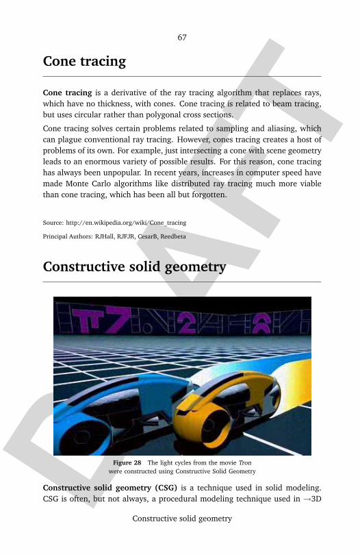
DRAF

T

67

Constructive solid geometry

Cone tracing

Cone tracing is a derivative of the ray tracing algorithm that replaces rays,which have no thickness, with cones. Cone tracing is related to beam tracing,but uses circular rather than polygonal cross sections.

Cone tracing solves certain problems related to sampling and aliasing, whichcan plague conventional ray tracing. However, cones tracing creates a host ofproblems of its own. For example, just intersecting a cone with scene geometryleads to an enormous variety of possible results. For this reason, cone tracinghas always been unpopular. In recent years, increases in computer speed havemade Monte Carlo algorithms like distributed ray tracing much more viablethan cone tracing, which has been all but forgotten.

Source: http://en.wikipedia.org/wiki/Cone_tracing

Principal Authors: RJHall, RJFJR, CesarB, Reedbeta


Figure 28 The light cycles from the movie Tronwere constructed using Constructive Solid Geometry

Constructive solid geometry (CSG) is a technique used in solid modeling.CSG is often, but not always, a procedural modeling technique used in →3D

DRAF

T

68


computer graphics and CAD. Constructive solid geometry allows a modelerto create a complex surface or object by using Boolean operators to combineobjects. Often CSG presents a model or surface that appears visually complex,but is actually little more than cleverly combined or decombined objects. (Insome cases, constructive solid geometry is performed on polygonal meshes,and may or may not be procedural and/or parametric.)

The simplest solid objects used for the representation are called primitives.Typically they are the objects of simple shape: cuboids, cylinders, prisms, pyra-mids, spheres, cones. The set of allowable primitives is limited by each soft-ware package. Some software packages allow CSG on curved objects whileother packages do not.

It is said that an object is constructed from primitives by means of allowableoperations, which are typically Boolean operations on sets: union, intersectionand difference.

OperationsIn modeling packages, basic geometric objects such as the cube or ’box’, sphereor ellipse, torus, and a number of other shapes that can be described using amathematical formula, are commonly known as primitives. These objects cantypically be described by a procedure which accepts some number of parame-ters; for example, a sphere may be described by the coordinates of its centerpoint, along with a radius value. These primitives can be combined into com-pound objects using operations like these:

Boolean union Boolean difference Boolean intersection

The merger of two objects intoone.

The subtraction of one objectfrom another.

The portion common to bothobjects.

Table 1 Operations in constructive solid geometry

DRAF

T

69

Conversion between quaternions and Euler angles

Applications of CSGConstructive solid geometry has a number of practical uses. It is used in caseswhere simple geometric objects are desired, or where mathematical accuracyis important. The Unreal engine uses this system, as do Hammer (the mappingengine for the Source engine) and Quake. (Hammer actually started out as aneditor for Quake.) BRL-CAD is a solid modeling CAD package that is fundamen-tally based on CSG modeling techniques. CSG is popular because a modelercan use a set of relatively simple objects to create very complicated geometry.When CSG is procedural or parametric, the user can revise their complex geom-etry by changing the position of objects or by changing the Boolean operationused to combine those objects.

Source: http://en.wikipedia.org/wiki/Constructive_solid_geometry

Principal Authors: Oleg Alexandrov, Mikkalai, Michael Hardy, Operativem, Merovingian

Conversion between quaternions and Eu-ler angles

Spatial rotations in three dimensions can be parametrized using both Euler an-gles and unit quaternions. This article explains how to convert between thetwo representations. Actually this simple use of "quaternions" was first pre-sented by Euler some seventy years earlier than Hamilton to solve the problemof "magic squares." For this reason the dynamics community commonly refersto quaternions in this application as "Euler parameters".

A unit quaternion can be described as:

q =

[

q0 q1 q2 q3

]T

|q|2 = q20 + q21 + q22 + q23 = 1

q0 = cos(α/2)

q1 = sin(α/2) cos(βx)

q2 = sin(α/2) cos(βy)

DRAF

T

70

Conversion between quaternions and Euler angles

q3 = sin(α/2) cos(βz)

where α is a simple rotation angle and βx, βy , βz , are the "direction cosines"locating the axis of rotation (Euler’s Theorem).

Figure 29

Similarly for Euler angles, we use (in terms of flight dynamics):

• Roll - φ: rotation about the X-axis• Pitch - θ: rotation about the Y-axis• Yaw - ψ: rotation about the Z-axis

where the X-axis points forward, Y-axis to the right and Z-axis downward andin the example to follow the rotation occurs in the order yaw, pitch, roll (aboutbody-fixed axes).

Rotation matricesThe orthogonal matrix corresponding to a rotation by the unit quaternion q isgiven by

1 − 2(q2

2+ q

2

3) 2(q1q2 − q0q3) 2(q0q2 + q1q3)

2(q1q2 + q0q3) 1 − 2(q2

1+ q

2

3) 2(q2q3 − q0q1)

2(q1q3 − q0q2) 2(q0q1 + q2q3) 1 − 2(q2

1+ q

2

2)

The orthogonal matrix corresponding to a rotation with Euler angles φ, θ ψ, isgiven by

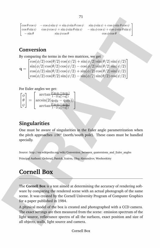
DRAF

T

71

Cornell Box

cos θ cosψ − cosφ sinψ + sinφ sin θ cosψ sinφ sinψ + cosφ sin θ cosψ

cos θ sinψ cosφ cosψ + sinφ sin θ sinψ − sinφ cosψ + cosφ sin θ sinψ

− sin θ sinφ cos θ cosφ cos θ

ConversionBy comparing the terms in the two matrices, we get

q =

cos(φ/2) cos(θ/2) cos(ψ/2) + sin(φ/2) sin(θ/2) sin(ψ/2)sin(φ/2) cos(θ/2) cos(ψ/2) − cos(φ/2) sin(θ/2) sin(ψ/2)cos(φ/2) sin(θ/2) cos(ψ/2) + sin(φ/2) cos(θ/2) sin(ψ/2)cos(φ/2) cos(θ/2) sin(ψ/2) − sin(φ/2) sin(θ/2) cos(ψ/2)

For Euler angles we get:

φ

θ

ψ

=

arctan2(q0q1+q2q3)1−2(q2

1+q

2

2)

arcsin(2(q0q2 − q3q1))

arctan2(q0q3+q1q2)1−2(q2

2+q

2

3)

SingularitiesOne must be aware of singularities in the Euler angle parametrization whenthe pitch approaches ±90o (north/south pole). These cases must be handledspecially.

Source: http://en.wikipedia.org/wiki/Conversion_between_quaternions_and_Euler_angles

Principal Authors: Orderud, Patrick, Icairns, Oleg Alexandrov, Woohookitty

Cornell Box

The Cornell Box is a test aimed at determining the accuracy of rendering soft-ware by comparing the rendered scene with an actual photograph of the samescene. It was created by the Cornell University Program of Computer Graphicsfor a paper published in 1984.

A physical model of the box is created and photographed with a CCD camera.The exact settings are then measured from the scene: emission spectrum of thelight source, reflectance spectra of all the surfaces, exact position and size ofall objects, walls, light source and camera.

DRAF

T

72

Cornell Box

Figure 30 Standard Cornell Box rendered with POV-Ray

The same scene is then reproduced in the renderer, and the output file is com-pared with the photography.

The basic environment consists of:

• One light source in the center of a white ceiling• A green right wall• A red left wall• A white back wall• A white floor

Objects are often placed inside the box. The first objects placed inside theenvironment were two white boxes. Another common version first used to testphoton mapping includes two spheres: one with a perfect mirror surface andone made of glass.

The physical properties of the box are designed to show diffuse interreflection.For example, some light should reflect off the red and green walls and bounceonto the white walls, so parts of the white walls should appear slightly red orgreen.

DRAF

T

73

Crowd simulation

Today, the Cornell Box is often used to show off renderers in a similar way asthe Stanford Bunny, the →Utah teapot, and Lenna: computer scientists oftenuse the scene just for its visual properties without comparing it to test datafrom a physical model.

See also

• →Utah teapot• Lenna• Stanford Bunny• Suzanne

External links

• The Cornell Box website54

Source: http://en.wikipedia.org/wiki/Cornell_Box

Principal Authors: SeeSchloss, T-tus, John Fader, 1983, Reedbeta

Crowd simulation

Crowd simulation is the process of simulating the movement of a large num-ber of objects or characters, now often appearing in →3D computer graphicsfor film.

The need for crowd simulation arises when a scene calls for more charactersthan can be practically animated using conventional systems, such as skele-tons/bones.

Animators typically create a library of motions, either for the entire charac-ter or for individual body parts. To simplify processing, these animations aresometimes baked as morphs. Alternatively, the motions can be generated pro-cedurally - i.e. choreographed automatically by software.

The actual movement and interactions of the crowd is typically done in one oftwo ways:

• Particle Motion: The characters are attached to point particles, which arethen animated by simulating wind, gravity, attractions, and collisions. The

http://www.graphics.cornell.edu/online/box/54

DRAF

T

74

Crowd simulation

particle method is usually inexpensive to implement, and can be done inmost 3D software packages. However, the method is not very realistic be-cause it is difficult to direct individual entities when necessary, and becausemotion is generally limited to a flat surface.

• Crowd AI : The entities - also called agents - are given artificial intelligence,which guides the entities based on one or more of sight, hearing, basicemotion, energy level, aggressiveness level, etc.. The entities are givengoals and then interact with each other as members of a real crowd would.They are often programmed to respond to changes in environment, en-abling them to climb hills, jump over holes, scale ladders, etc. This systemis much more realistic than particle motion, but is very expensive to pro-gram and implement.

The most notable examples of AI simulation can be seen in New Line Cinema’sThe Lord of the Rings films, where AI armies of many thousands battle eachother. The crowd simulation was done using Weta Digital’s MASSIVE software.Crowd simulation can also refer to simulations based on group dynamics andcrowd psychology, often in public safety planning. In this case, the focus is justthe behavior of the crowd, and not the visual realism of the simulation.

See also

• →3D computer graphics• Artificial intelligence• Emergent behavior• MASSIVE (animation)• Multi-agent system• →Particle system

External links

• NetLogo55, a free software for multi-agent modeling, simulation, and thelike.

• MASSIVE56, the software used in The Lord of the Rings films.

Source: http://en.wikipedia.org/wiki/Crowd_simulation

Principal Authors: Aniboy2000, The Anome, Pmkpmk, Kuru, JonHarder

http://ccl.northwestern.edu/netlogo55

http://massivesoftware.com56

DRAF

T

75

Diffuse reflection

Cube mapping

In computer graphics, cube mapping is a technique that takes a three dimen-sional texture coordinate and returns a texel from a given cube map (verysimilar to a skybox’s texture’s format). This texture coordinate is a vector thatspecifies which way to look from the center of the cube mapped cube to get thedesired texel.

See also:

• Skybox (video games)• Cube mapped reflection

Source: http://en.wikipedia.org/wiki/Cube_mapping

Principal Authors: TopherTG

Diffuse reflection

Diffuse reflection is the reflection of light from an uneven or granular surfacesuch that an incident ray is seemingly reflected at a number of angles. It isthe complement to specular reflection. If a surface is completely nonspecular,

DRAF

T

76

Digital puppetry

the reflected light will be evenly spread over the hemisphere surrounding thesurface (2×π steradians).

The most familiar example of the distinction between specular and diffuse re-flection would be matte and glossy paints as used in home painting. Mattepaints have a higher proportion of diffuse reflection, while gloss paints have agreater part of specular reflection.

Diffuse interreflection is a process whereby light reflected from an objectstrikes other objects in the surrounding area, illuminating them. Diffuse in-terreflection specifically describes light reflected from objects which are notshiny or specular. In real life terms what this means is that light is reflectedoff non-shiny surfaces such as the ground, walls, or fabric, to reach areas notdirectly in view of a light source. If the diffuse surface is colored, the reflectedlight is also colored, resulting in similar coloration of surrounding objects.

In →3D computer graphics, diffuse interreflection is an important componentof global illumination. There are a number of ways to model diffuse inter-reflection when rendering a scene. →Radiosity and photon mapping are twocommonly used methods.

See also

• Optics• Reflectivity• Specular reflection• →Lambertian reflectance

Source: http://en.wikipedia.org/wiki/Diffuse_reflection

Principal Authors: JohnOwens, Srleffler, Patrick, Francs2000, Flamurai

Digital puppetry

Digital puppetry is the manipulation and performance of digitally animated2D or 3D figures and objects in a virtual environment that are rendered in real-time by computers. It is most commonly used in film and television production,but has also been utilized in interactive theme park attractions and live theatre.

The exact definition of what is and is not digital puppetry is subject to debatewithin the puppetry and computer graphics communities, but it is generallyagreed that digital puppetry differs from conventional computer animation in

DRAF

T

77

Digital puppetry

that it involves performing characters in real time, rather than animating themframe by frame.

Digital puppetry is closely associated with motion capture technologies and 3Danimation. It is sometimes referred to as Performance Animation. Machinimais a form of digital puppetry, although most machinima creators do not identifythemselves as puppeteers.

History & UsageDigital puppetry was pioneered by the late Jim Henson, creator of The Mup-pets. The character Waldo C. Graphic in the Muppet television series The JimHenson Hour is widely regarded to have been the first example of a digitallyanimated figure being performed and rendered in real-time on television andgrew out of experiments Henson conducted in 1987 with a computer generat-ed version of Kermit the Frog for InnerTube, which was the unaired televisionpilot for Jim Henson Hour.

Another early digital puppet was Mike Normal, which was developed by com-puter graphics company deGraf/Wahrman and was first demonstrated at the1988 SIGGRAPH convention. The system developed by deGraf/Wahrman toperform Mike Normal was later used to create a representation of the villainCain in the motion picture RoboCop 2, which is believed to be the first exam-ple of digital puppetry being used to create a character in a full-length motionpicture.

In 1994, the BBC introduced a live digital puppet cat called Ratz, in the TVshow Live & Kicking. He became the first real-time rendered digital puppet toappear on live TV. He also co-presented Children’s BBC, and was eventuallygiven his own show, RatzRun.

A more recent example of digital puppetry from 2003 is "Bugs Live", a digitalpuppet of Bugs Bunny created by Phillip Reay for Warner Brothers Pictures.The puppet was created using hand drawn frames of animation that were pup-peteered by Bruce Lanoil and David Barclay. The Bugs Live puppet was used tocreate nearly 900 minutes of live, fully interactive interviews of 2D animatedBugs character about his role in then recent movie Looney Tunes: Back In Ac-tion in English and Spanish. Bugs Live also appeared at the 2004 SIGGRAPHDigital Puppetry Special Session with the Muppet puppet Gonzo.

In 2004 Walt Disney Imagineering used digital puppetry techniques to createthe Turtle Talk with Crush attractions at the Walt Disney World and Disney’sCalifornia Adventure theme parks. In the attraction, a hidden puppeteer per-forms and voices a digital puppet of Crush, the laid-back sea turtle from FindingNemo, on a large rear-projection screen. To the audience Crush appears to be

DRAF

T

78

Digital puppetry

swimming inside an aquarium and engages in unscripted, real-time conversa-tions with theme park guests.

Types of Digital PuppetryWaldo Puppetry - A digital puppet is controlled onscreen by a puppeteer whouses a telemetric input device connected to the computer. The X-Y-Z axis move-ment of the input device causes the digital puppet to move correspondingly. Akeyboard is sometimes used in place of a telemetric input device.

Motion Capture Puppetry (Mocap Puppetry) - An object (puppet) or humanbody is used as a physical representation of a digital puppet and manipulatedby a puppeteer. The movements of the object or body are matched correspond-ingly by the digital puppet in real-time.

Machinima - A production technique that can be used to perform digitalpuppets. Machinima as a production technique concerns the rendering ofcomputer-generated imagery (CGI) using low-end 3D engines in video games.Players act out scenes in real-time using characters and settings within a gameand the resulting footage is recorded and later edited in to a finished film.

See also

• →Motion capture• Machinima• Puppets• Puppeteer

External links

• Machin-X57 - Discussion of theories, tools and applications of digital pup-petry as well as news from the digital puppetry community.

• Machinima.com58 - Large web portal for machinima.

Source: http://en.wikipedia.org/wiki/Digital_puppetry

http://machin-x.blogspot.com57

http://www.machinima.com58

DRAF

T

79

Direct3D

Dilution of precision (computer graphics)

Dilution of precision is an algorithmic trick used to handle difficult problemsin hidden line removal, caused when horizontal and vertical edges lay on topof each other due to numerical instability. Numerically, the severity escalateswhen a CAD model is viewed along the principal axii or when a geometric formis viewed end-on. The trick is to alter the view vector by a small amount, there-by hiding the flaws. Unfortunately, this mathematical modification introducesnew issues of its own, namely that the exact nature of the original problem hasbeen destroyed, and visible artifacts of this kluge will continue to haunt thealgorithm. One such issue is that edges that were well defined and hidden willnow be problematic. Another common issue is that the bottom edges on circlesviewed end-on will often become visible and propagate their visibility thoughtthe problem.

External link

Source: http://en.wikipedia.org/wiki/Dilution_of_precision_%28computer_graphics%29

Principal Authors: Wheger, David Levy, RJHall, Whitepaw

Direct3D

Direct3D is part of Microsoft’s DirectX API. Direct3D is only available for Mi-crosoft’s various Windows operating systems (Windows 95 and above) andis the base for the graphics API on the Xbox and Xbox 360 console systems.Direct3D is used to render three dimensional graphics in applications whereperformance is important, such as games. Direct3D also allows applications torun fullscreen instead of embedded in a window, though they can still run in awindow if programmed for that feature. Direct3D uses hardware accelerationif it is available on the graphic board.

Direct3D is a 3D API. That is, it contains many commands for 3D rendering,but contains few commands for rendering 2D graphics.59 Microsoft strives tocontinually update Direct3D to support the latest technology available on 3Dgraphics cards. Direct3D offers full vertex software emulation but no pixel

Microsoft DirectX SDK Readme (December 2005)(http://msdn.microsoft.com/directx/sdk/read-59

mepage/default.aspx)

DRAF

T

80

Direct3D

software emulation for features not available in hardware. For example, if aprogram programmed using Direct3D requires pixel shaders and the graphicscard on the user’s computer does not support that feature, Direct3D will notemulate it. The program will most likely exit with an error message. The APIdoes define a Reference Rasterizer (or REF device), which emulates a genericgraphics card, although it’s too slow to be used in any application to emulatepixel shaders and is usually ignored.

Direct3D’s main competitor is →OpenGL. There are numerous features andissues that proponents for either API disagree over, see comparison of Direct3Dand OpenGL for a summary.

Version historyIn 1992, Servan Keondjian started a company named RenderMorphics, whichdeveloped a 3D graphics API named Reality Lab, which was used in medicalimaging and CAD software. Two versions of this API were released. Microsoftbought RenderMorphics in February 1995, bringing Keondjian on board to im-plement a 3D graphics engine for Windows 95. This resulted in the first versionof Direct3D.

In DirectX version 7.0, the .dds texture format was introduced.

As of DirectX version 8.0, Direct3D was rolled up into a package called Direc-tX Graphics. DirectX Graphics was meant to be a combination of DirectDrawand Direct3D, but in reality was just Direct3D with a few DirectDraw featuresadded. Most users still refer to DirectX Graphics as Direct3D.

Direct3D was not considered to be user friendly, but as of DirectX version 8.1,many usability problems were resolved. Direct3D (DX8) contained many verypowerful 3D graphics features, such as vertex shaders, pixel shaders, fog, bumpmapping and texture mapping.

DirectX version 9.0 added a new version of the →High Level Shader Language,support for high dynamic range lighting, multiple render targets, and vertexbuffer indexing.

Direct3D 10Microsoft is currently working on a large update to Direct3D API. Originallycalled Windows Graphics Foundation, DirectX 10, and later DirectX Next, butcurrently referred to as Direct3D 10, it will appear as part of Windows Vista.Version 10 will represent a departure from the driver model of DirectX Graph-ics 9.0, with the addition of a scheduler and memory virtualization system.Direct3D 10 will forego the current DirectX practice of using "capability bits" toindicate which features are active on the current hardware. Instead, Direct3D

DRAF

T

81

Direct3D

10 will define a minimum standard of hardware capabilities which must besupported for a display system to be "Direct3D 10 compatible". According toMicrosoft, Direct3D 10 will be able to display graphics up to 8 times morequickly than DirectX Graphics 9.0c. In addition, Direct3D 10 will incorporateMicrosoft Shader Model 4.0.

Vista will ship with Windows Graphics Foundation (WGF) 1.0. WGF 2.0 willship later (after Vista). Beneath the WGF is either legacy (XP) drivers with lim-ited functionality or Windows Display Driver Model (WDDM) drivers in one oftwo flavors: Basic (for existing hardware) and Advanced (for post-Vista hard-ware). What’s currently referred to as DX10 is really WGF 2.0 atop AdvancedWDDM drivers running on post-Vista hardware. WGF 1.0 (atop either flavorof WDDM), as shipping with Vista, is referred to by MS as DX9.L – it’s mostdefinitely not DX10. It certainly does have some benefits – managed resourcesfor "unlimited" memory (limited by virtual memory), better gamma controland text rendering, some performance improvements, etc – but it’s a relativelyminor upgrade, and it’s not going to drive radical new development in eithergames or GPUs.

DX10 functionality will require WGF 2.0, and will require the Advanced WD-DM, which in turn will require new graphics hardware, even beyond uni-fied shaders and an updated shader model: it includes things like additionalpipeline stages (geometry shaders), hardware virtualization (to allow multiplethreads/processes time-sliced use of the GPU), demand-paged virtual graphicsmemory, offload of various operations from the CPU to the GPU, and more. NoGPU is going to be available with the full WGF 2.0 featureset in 2006.

Note also that games that take advantage of WGF 1.0 will run successfully onVista atop existing hardware. However, once they make the transition to WGF2.0 it’s unclear if they’ll be able to degrade gracefully to 1.0, meaning that thefirst "must have" game using WGF 2.0 is going to require not just Vista but anew video card: while there will be XP drivers for "DX10" hardware XP won’tsupport WGF 2.0, and older cards running Vista will at most support WGF 1.0and Basic WDDM drivers. So the first WGF 2.0 games will be looking at a fairlysmall market with the requisite hardware base, and thus there may be a bit ofdelay until such titles are released (fortunately the new hardware should offerenough of an improvement on existing titles that we won’t see a chicken-and-egg situation develop).

New Features

DRAF

T

82

Direct3D

• Fixed pipeline60 is being done away with in favor of a fully programmablepipeline (often referred to as a unified pipeline architecture), which can beprogrammed to emulate the same.

• Paging of graphics memory, to allow data to be loaded to Video RAM whenneeded and move it out when not needed. This enables usage of the systemmemory to hold graphics data, such as textures, thereby allowing use ofmore and higher resolution textures in games.

• There is no limit on the number of objects which can be rendered, providedenough resources are available.61

• Virtualization of the graphics hardware, to allow multiplethreads/processes to use it, in turns.

• New state object to enable the GPU to change states efficiently.• Shader Model 4.0, enhances the programmability of the graphics pipeline.

It adds instructions for integer and bitwise calculations.• Geometry shaders, which work on indivdual triangles which form a mesh.• Texture arrays enable swapping of textures in GPU without CPU interven-

tion.• Resource View enables pre-caching of resources, thereby reducing latency.• Predicated Rendering allows drawing calls to be ignored based on some

other conditions. This enables rapid occlusion culling, which prevents ob-jects from being rendered if it is not visible or too far to be visible.

Related toolsDirectX comes with D3DX, a library of tools designed to perform commonmathematical calculations and several more complicated tasks, such as compil-ing or assembling shaders used for 3D graphic programming. It also includesseveral classes that simplify the use of 3D-models and, for example, particlesystems. D3DX is provided as a dynamic link library (DLL).

DXUT (also called the sample framework) is a layer built on top of the Direct3DAPI. The framework is designed to help the programmer spend less time withmundane tasks, such as creating a window, creating a device, processing Win-dows messages and handling device events.

CNet News(http://news.com.com/An+inside+look+at+Windows+Vista+-+page+4/2100-104360

_3-6051736-4.html?tag=st.num)SDK March 2006(http://www.ati.com/developer/radeonSDK.html?tag=Radeon)61

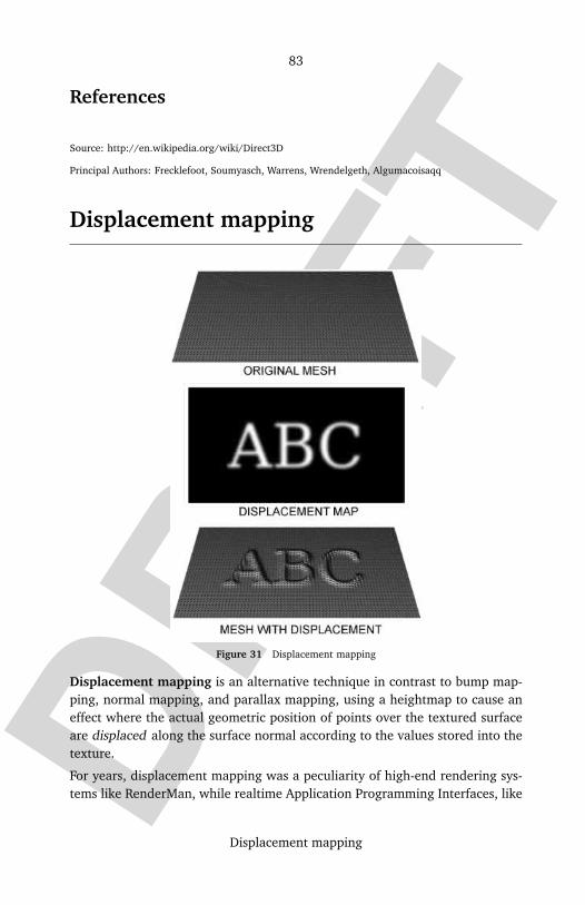
DRAF

T

83

Displacement mapping

References

Source: http://en.wikipedia.org/wiki/Direct3D

Principal Authors: Frecklefoot, Soumyasch, Warrens, Wrendelgeth, Algumacoisaqq


Figure 31 Displacement mapping

Displacement mapping is an alternative technique in contrast to bump map-ping, normal mapping, and parallax mapping, using a heightmap to cause aneffect where the actual geometric position of points over the textured surfaceare displaced along the surface normal according to the values stored into thetexture.

For years, displacement mapping was a peculiarity of high-end rendering sys-tems like RenderMan, while realtime Application Programming Interfaces, like

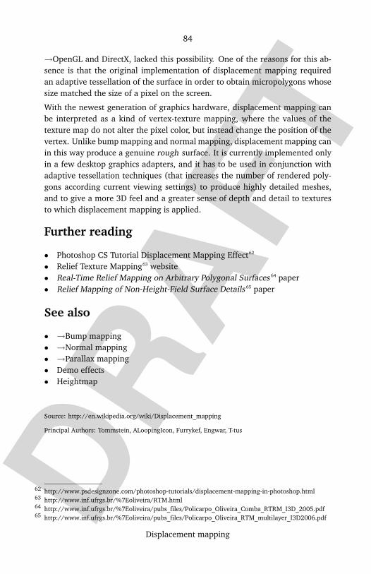
DRAF

T

84


→OpenGL and DirectX, lacked this possibility. One of the reasons for this ab-sence is that the original implementation of displacement mapping requiredan adaptive tessellation of the surface in order to obtain micropolygons whosesize matched the size of a pixel on the screen.

With the newest generation of graphics hardware, displacement mapping canbe interpreted as a kind of vertex-texture mapping, where the values of thetexture map do not alter the pixel color, but instead change the position of thevertex. Unlike bump mapping and normal mapping, displacement mapping canin this way produce a genuine rough surface. It is currently implemented onlyin a few desktop graphics adapters, and it has to be used in conjunction withadaptive tessellation techniques (that increases the number of rendered poly-gons according current viewing settings) to produce highly detailed meshes,and to give a more 3D feel and a greater sense of depth and detail to texturesto which displacement mapping is applied.

Further reading

• Photoshop CS Tutorial Displacement Mapping Effect62

• Relief Texture Mapping63 website• Real-Time Relief Mapping on Arbitrary Polygonal Surfaces 64 paper• Relief Mapping of Non-Height-Field Surface Details 65 paper

See also

• →Bump mapping• →Normal mapping• →Parallax mapping• Demo effects• Heightmap

Source: http://en.wikipedia.org/wiki/Displacement_mapping

Principal Authors: Tommstein, ALoopingIcon, Furrykef, Engwar, T-tus

http://www.psdesignzone.com/photoshop-tutorials/displacement-mapping-in-photoshop.html62

http://www.inf.ufrgs.br/%7Eoliveira/RTM.html63

http://www.inf.ufrgs.br/%7Eoliveira/pubs_files/Policarpo_Oliveira_Comba_RTRM_I3D_2005.pdf64

http://www.inf.ufrgs.br/%7Eoliveira/pubs_files/Policarpo_Oliveira_RTM_multilayer_I3D2006.pdf65

DRAF

T

85

Distance fog

Distance fog

Distance fog is a technique used in →3D computer graphics to enhance theperception of distance.

Because many of the shapes in graphical environments are relatively simple,and complex shadows are difficult to render, many graphics engines employ a"fog" gradient, so that objects further from the camera are progressively moreobscured by haze. This technique works because of light scattering, whichcauses more distant objects to appear hazier to the eye, especially in outdoorenvironments.

Figure 32 Example of fog

Fogging is another use of distance fog in mid to late nineties games, whereprocessing power was not enough to render far viewing distances, and clippingwas employed. However, the effect could be very distracting, and by applying amedium-ranged fog, the clipped polygons would fade in more realistically fromthe haze, even though the effect may have been considered unrealistic in somecases. Many early Nintendo 64 games used this effect — most (in)famously inTurok: Dinosaur Hunter and Superman 64.

See also

• Computer graphics• Virtual reality

Source: http://en.wikipedia.org/wiki/Distance_fog

Principal Authors: Graft, SimonP, Reedbeta, WolfenSilva, RJHall

DRAF

T

86

Draw distance

Draw distance

Draw distance is a computer graphics term, defined as the distance in a 3dimensional scene that is still drawn by the rendering engine. Polygons that liebehind the draw distance won’t be drawn to the screen.

As the draw distance increases more polygons need to be drawn onto the screenwhich requires more computing power. This means the graphic quality andrealism of the scene will increase as draw distance increases, but the overallperformance (frames per second) will decrease. Many games and applicationswill allow users to manually set the draw distance to balance performance andvisuals.

Older games had far shorter draw distances, most noticeable in vast, openscenes. Racing arcade games were particularly infamous, as the open high-ways and roads often led to "pop-up graphics" - an effect where distant objectssuddenly appear without warning as the camera gets closer to it. This is a hall-mark of poor draw distance, and still plagues large, open-ended games like theGrand Theft Auto series.

A common trick used in games to disguise a short draw distance is to obscurethe area with a distance fog. Alternative methods have been developed tosidestep the problem altogether using level of detail manipulation. Black &White was one of the earlier games to use adaptive level of detail to decreasethe number of polygons in objects as they moved away from the camera, al-lowing it to have a massive draw distance while maintaining detail in close-upviews.

Grand Theft Auto 3 made particular use of fogging, however, this made thegame less playable when driving or flying at high speed, as object would pop-up out of the fog and cause you to crash into them.

Source: http://en.wikipedia.org/wiki/Draw_distance

Principal Authors: Goncalopp, 25, Deepomega, Oswax, Xhin

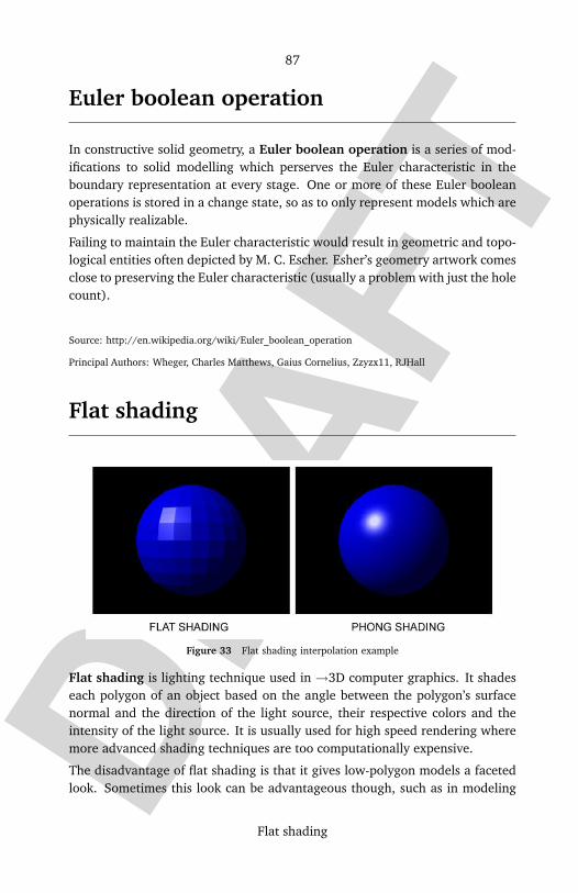
DRAF

T

87

Flat shading

Euler boolean operation

In constructive solid geometry, a Euler boolean operation is a series of mod-ifications to solid modelling which perserves the Euler characteristic in theboundary representation at every stage. One or more of these Euler booleanoperations is stored in a change state, so as to only represent models which arephysically realizable.

Failing to maintain the Euler characteristic would result in geometric and topo-logical entities often depicted by M. C. Escher. Esher’s geometry artwork comesclose to preserving the Euler characteristic (usually a problem with just the holecount).

Source: http://en.wikipedia.org/wiki/Euler_boolean_operation

Principal Authors: Wheger, Charles Matthews, Gaius Cornelius, Zzyzx11, RJHall

Flat shading

Figure 33 Flat shading interpolation example

Flat shading is lighting technique used in →3D computer graphics. It shadeseach polygon of an object based on the angle between the polygon’s surfacenormal and the direction of the light source, their respective colors and theintensity of the light source. It is usually used for high speed rendering wheremore advanced shading techniques are too computationally expensive.

The disadvantage of flat shading is that it gives low-polygon models a facetedlook. Sometimes this look can be advantageous though, such as in modeling

DRAF

T

88

Forward kinematic animation

boxy objects. Artists sometimes use flat shading to look at the polygons of a sol-id model they are creating. More advanced and realistic lighting and shadingtechniques include →Gouraud shading and →Phong shading.

See also: computer graphics

Source: http://en.wikipedia.org/wiki/Flat_shading

Principal Authors: RJFJR, Mrwojo, AndreasB, Poccil, Whitepaw, D3

Forward kinematic animation

Forward kinematic animation is a method in →3D computer graphics foranimating models.

The essential concept of forward kinematic animation is that the positions ofparticular parts of the model at a specified time are calculated from the positionand orientation of the object, together with any information on the joints of anarticulated model. So for example if the object to be animated is an arm withthe shoulder remaining at a fixed location, the location of the tip of the thumbwould be calculated from the angles of the shoulder, elbow, wrist, thumb andknuckle joints. Three of these joints (the shoulder, wrist and the base of thethumb) have more than one degree of freedom, all of which must be takeninto account. If the model were an entire human figure, then the location ofthe shoulder would also have to be calculated from other properties of themodel.

Forward kinematic animation can be distinguished from inverse kinematic an-imation by this means of calculation - in inverse kinematics the orientation ofarticulated parts is calculated from the desired position of certain points on themodel. It is also distinguished from other animation systems by the fact thatthe motion of the model is defined directly by the animator - no account istaken of any physical laws that might be in effect on the model, such as gravityor collision with other models.

Source: http://en.wikipedia.org/wiki/Forward_kinematic_animation

Principal Authors: Onebyone, Jiang, TimBentley, Charles Matthews, Bryan Derksen

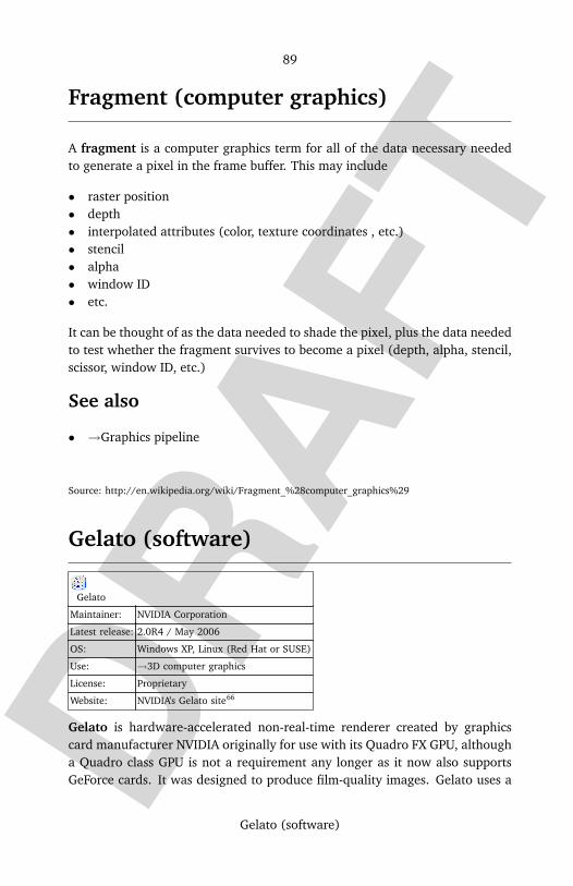
DRAF

T

89

Gelato (software)

Fragment (computer graphics)

A fragment is a computer graphics term for all of the data necessary neededto generate a pixel in the frame buffer. This may include

• raster position• depth• interpolated attributes (color, texture coordinates , etc.)• stencil• alpha• window ID• etc.

It can be thought of as the data needed to shade the pixel, plus the data neededto test whether the fragment survives to become a pixel (depth, alpha, stencil,scissor, window ID, etc.)

See also

• →Graphics pipeline

Source: http://en.wikipedia.org/wiki/Fragment_%28computer_graphics%29

Gelato (software)

Gelato

Maintainer: NVIDIA Corporation

Latest release: 2.0R4 / May 2006

OS: Windows XP, Linux (Red Hat or SUSE)

Use: →3D computer graphics

License: Proprietary

Website: NVIDIA’s Gelato site66

Gelato is hardware-accelerated non-real-time renderer created by graphicscard manufacturer NVIDIA originally for use with its Quadro FX GPU, althougha Quadro class GPU is not a requirement any longer as it now also supportsGeForce cards. It was designed to produce film-quality images. Gelato uses a

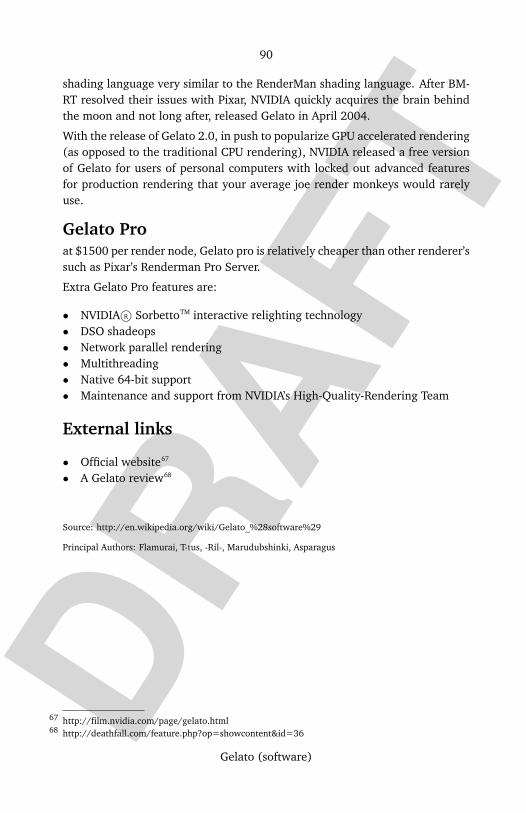
DRAF

T

90

Gelato (software)

shading language very similar to the RenderMan shading language. After BM-RT resolved their issues with Pixar, NVIDIA quickly acquires the brain behindthe moon and not long after, released Gelato in April 2004.

With the release of Gelato 2.0, in push to popularize GPU accelerated rendering(as opposed to the traditional CPU rendering), NVIDIA released a free versionof Gelato for users of personal computers with locked out advanced featuresfor production rendering that your average joe render monkeys would rarelyuse.

Gelato Proat $1500 per render node, Gelato pro is relatively cheaper than other renderer’ssuch as Pixar’s Renderman Pro Server.

Extra Gelato Pro features are:

• NVIDIA R© SorbettoTM interactive relighting technology• DSO shadeops• Network parallel rendering• Multithreading• Native 64-bit support• Maintenance and support from NVIDIA’s High-Quality-Rendering Team

External links

• Official website67

• A Gelato review68

Source: http://en.wikipedia.org/wiki/Gelato_%28software%29

Principal Authors: Flamurai, T-tus, -Ril-, Marudubshinki, Asparagus

http://film.nvidia.com/page/gelato.html67

http://deathfall.com/feature.php?op=showcontent&id=3668

DRAF

T

91

Geometric model

Geometric model

A geometric model describes the shape of a physical or mathematical objectby means of geometric concepts. Geometric model(l)ing is the constructionor use of geometric models. Geometric models are used in computer graphics,computer-aided design and manufacturing, and many applied fields such asmedical image processing.

Geometric models can be built for objects of any dimension in any geometricspace. Both 2D and 3D geometric models are extensively used in comput-er graphics. 2D models are important in computer typography and technicaldrawing. 3D models are central to computer-aided design and manufacturing,and many applied technical fields such as geology and medical image process-ing.

Geometric models are usually distinguished from procedural and object-oriented models, which define the shape implicitly by an algorithm. They arealso contrasted with digital images and volumetric models; and with implicitmathematical models such as the zero set of an arbitrary polynomial. How-ever, the distinction is often blurred: for instance, geometric shapes can berepresented by objects; a digital image can be interpreted as a collection ofcolored squares; and geometric shapes such as circles are defined by implicitmathematical equations. Also, the modeling of fractal objects often requires acombination of geometric and procedural techniques.

See also

• Computational geometry

Source: http://en.wikipedia.org/wiki/Geometric_model

Principal Authors: Oleg Alexandrov, Mdd, Jorge Stolfi, Kbdank71, Patrick

DRAF

T

92

Geometry Processing

Geometry pipelines

Geometry Pipelines, also called Geometry Engines (GE) are the first stage in aclassical Graphics Pipeline, such as the Reality Engine. They do the transforma-tion from 3D coordinates used to specify the geometry to a unified coordinatesystem used by the Raster Manager (RM) to rasterize the geometry into frame-buffer pixels. The Display Generator (DG) scans these pixels into a video signalunderstood by a monitor. In →OpenGL, this transformation is defined by theModelview Matrix and the Projection Matrix. Typically, the modelview matrixdefines the transformation of the incoming vertices into world coordinates, acoordinate system used for all vertices. The projection matrix defines how this3-dimensional coordinate space is projected to the Viewport. In addition to thistransformation, the GEs compute the vertex colors based on the light settings,may perform texture coordinate generation as well as clipping of the geometry.The Geforce graphics cards from nVidia introduced these functionalities for thefirst time in the consumer market, labelled as hardware-based Transform andLighting (T&L).

See also

• Computer graphics• James H. Clark• Silicon Graphics, Inc.

Source: http://en.wikipedia.org/wiki/Geometry_pipelines

Principal Authors: Jpbowen, Bumm13, JoJan, Joyous!

Geometry Processing

Geometry Processing is a fast-growing area of research that uses conceptsfrom applied mathematics, computer science, and engineering to design ef-ficient algorithms for the acquisition, reconstruction, analysis, manipulation,simulation and transmission of complex 3D models. Applications of geometryprocessing algorithms already cover a wide range of areas from multimedia,entertainment, and classical computer-aided design, to biomedical computing,reverse engineering, and scientific computing.

DRAF

T

93

GLEE

See also

• Computer-aided design (CAD)

External links

• " Digital Geometry Processing69", by Peter Schroder and Wim Sweldens

• Symposium on Geometry Processing70

• Multi-Res Modeling Group71, Caltech

• Compter Graphics & Multimedia Department72, RWTH-Aachen University

Source: http://en.wikipedia.org/wiki/Geometry_Processing

Principal Authors: Betamod, RJHall

GLEE

The OpenGL Easy Extension library (GLee) automatically links →OpenGL ex-tensions and core functions at initialisation time. This saves programmers theeffort of manually linking every required extension, and effectively brings theOpenGL library up to date.

GLee is compatible with Windows, Linux and FreeBSD platforms. It is alsolikely to be compatible with other unix-like systems which use X windows.

External links

Source: http://en.wikipedia.org/wiki/GLEE

http://www.multires.caltech.edu/pubs/DGPCourse/DGP.pdf69

http://www.geometryprocessing.org/70

http://www.multires.caltech.edu/71

http://www-i8.informatik.rwth-aachen.de/index.html72

DRAF

T

94

Glide API

GLEW

The OpenGL Extension Wrangler Library (GLEW) is a cross-platform C/C++library that helps in querying and loading →OpenGL extensions. GLEW pro-vides efficient run-time mechanisms for determining which OpenGL extensionsare supported on the target platform. all OpenGL extensions are exposed in asingle header file, which is machine-generated from the official extension list.GLEW is available for a variety of operating systems, including Windows, Lin-ux, Mac OS X, FreeBSD, Irix, and Solaris.

External linksGLEW English surname meaning wise. Believed to be from the wiseman of thetribe.Source: http://en.wikipedia.org/wiki/GLEW

Glide API

Glide was a proprietary 3D graphics API developed by 3dfx used on theirVoodoo graphics cards. It was dedicated to gaming performance, supportinggeometry and texture mapping primarily, in data formats identical to thoseused internally in their cards. The Voodoo cards were the first to offer per-formance to really make 3D games work well, and Glide became fairly widelyused as a result. The introduction of DirectX and full OpenGL implementationsfrom other vendors eventually doomed Glide, and 3dfx along with it.

Glide is based on the basic geometry and "world view" of →OpenGL. OpenGLis a very large library with about 250 calls in the API, many of which are oflimited use. Glide was an effort to select those features that were truly usefulfor gaming, leaving the rest out. The result was an API that was small enoughto be implemented entirely in hardware. That hardware, of course, was 3dfx’sown Voodoo cards. This led to several odd limitations in Glide – for instance,it only supported 16-bit color.

The combination of the Voodoo’s raw performance and Glide’s easy-to-use APIresulted in Voodoo cards generally dominating the gaming market from themid to late 1990s. The name Glide was chosen to be indicative of the GL un-derpinnings, while being different enough to avoid trademark problems. 3dfxalso supported a low-level MiniGL driver, making their cards particularly pop-ular for players of the various Quake-derived games. MiniGL was essentially a

DRAF

T

95

Global illumination

"different Glide" with a wider selection of OpenGL calls and lacking the dedi-cation to a single hardware platform. Due to the Voodoo’s "GL-like" hardware,MiniGL on Voodoo was very "thin" and ran almost as well as Glide.

As new cards entered the market 3dfx managed to hold the performance crownfor a short time, based largely on the tight integration between Glide andtheir hardware. This allowed them to be somewhat lax in hardware terms,which was important as the small gamer-only market 3dfx sold into wasn’tlarge enough to support a large development effort. It was not long beforeofferings from nVidia and ATI Technologies were able to outperform the latestVoodoo cards using standard APIs. 3dfx responded by releasing Glide as anopen source API, but it was too late. By late 1999 they announced that almostall games had moved to →Direct3D, and to a lesser extent, OpenGL.

Today old Glide supporting games can often be run on modern graphics cardswith help of a Glide wrapper. Numerous such computer programs exist.

External links

• GLIDE programming manual73

• Glide Wrappers74 at VoodooFiles

Source: http://en.wikipedia.org/wiki/Glide_API

Principal Authors: Maury Markowitz, Lproven, Doug Bell, The Anome, GreatWhiteNortherner

Global illumination

Global illumination algorithms used in →3D computer graphics are thosewhich, when determining the light falling on a surface, take into account notonly the light which has taken a path directly from a light source (direct illu-mination), but also light which has undergone reflection from other surfacesin the world (indirect illumination).

Images rendered using global illumination algorithms are more photorealisticthan images rendered using local illumination algorithms. However, they arealso much slower and more computationally expensive. A common approach isto compute the global illumination of a scene and store that information with

http://www.gamers.org/dEngine/xf3D/glide/glidepgm.htm73

http://www.voodoofiles.com/type.asp?cat_id=1474

DRAF

T

96

Global illumination

the geometry (ie. radiosity). That stored data can then be used to generate im-ages from different viewpoints for generating walkthroughs of a scene withouthaving to go through expensive lighting calculations.

→Radiosity, ray tracing, beam tracing, cone tracing, →Path Tracing, metropolislight transport and photon mapping are examples of algorithms used in globalillumination, some of which may be used together.

These algorithms model diffuse inter-reflection which is a very important partof global illumination, however most of these (excluding radiosity) also modelspecular reflection too which makes them more accurate algorithms to solvethe lighting equation and provide a more realistic globally illuminated scene.

The algorithms used to calculate the distribution of light energy between sur-faces of a scene are closely related to heat transfer simulations performed usingfinite-element methods in engineering design.

In real-time 3D graphics, global illumination is sometimes approximated by an"ambient" term in the lighting equation.

Figure 34 An example of a global illumination rendering, demonstrating how surface materialsare reflected in other surfaces.

See also

• Povray free rendering software featuring global illumination• YafRay free rendering software featuring global illumination• Radiance - highly accurate ray-tracing software system for UNIX computers.

Free to non-commercial users. It has been open-sourced.

DRAF

T

97

GLSL

External links

• PBRT75 - Literate programming, has a great accompanying book.• Vraywiki76 - Vraywiki website.• SplutterFish77 - developers of Brazil, a rendering system based on global

illumination. The site has an extensive gallery of contributed images• Perceptuum78 - good source for photon mapping, and other global illumina-

tion techniques.• Mental Images79 - makers of the MentalRay renderer. The renderer is used

in packages such as Softimage XSI, Maya and 3D Studio Max

Source: http://en.wikipedia.org/wiki/Global_illumination

Principal Authors: Dormant25, Reedbeta, Paranoid, Heron, Nohat, Jsnow, Peter bertok, Arru, RJHall,

Jose Ramos

GLSL

GLSL - OpenGL Shading Language also known as GLslang is a high levelshading language based on the C programming language. It was created by theOpenGL ARB for programming graphics processing units directly, thus givingdevelopers control of the graphics pipeline at the lowest level.

BackgroundWith the recent advancements in graphics cards, new features have been addedto allow for increased flexibility in the rendering pipeline at the vertex and frag-ment level. Programmability at this level is achieved with the use of fragmentand vertex shaders.

Originally, this functionality was achieved through the use of shaders written inassembly language. Assembly language is non-intuitive and rather complex fordevelopers to use. The OpenGL ARB created the OpenGL Shading Languageto provide a more intuitive method for programming the graphics processingunit while maintaining the open standards advantage that has driven OpenGLthroughout its history.

http://pbrt.org/75

http://www.vraywiki.com/76

http://www.splutterfish.com/77

http://www.hxa7241.org/perceptuum/perceptuum.html78

http://www.mentalimages.com/79

DRAF

T

98

GLSL

Originally introduced as an extension to OpenGL 1.5, the OpenGL ARB formal-ly included GLSL into the →OpenGL 2.0 core. →OpenGL 2.0 is the first majorrevision to →OpenGL since the creation of →OpenGL 1.0 in 1992.

Some benefits of using GLSL are:

• Cross platform compatibility on multiple operating systems, including Win-dows and Linux.

• The ability to write shaders that can be used on any hardware vendor’sgraphics card that supports the OpenGL Shading Language.

• Each hardware vendor includes the GLSL compiler in their driver, thus al-lowing each vendor to create code optimized for their particular graphicscard’s architecture.

Details

Data typesThe OpenGL Shading Language Specification defines 22 basic data types, someare the same as used in the C programming language, while others are specificto graphics processing.

• void – used for functions that do not return a value• bool – conditional type, values may be either true or false• int – a signed integer• float – a floating point number• vec2 – a 2 component floating point vector• vec3 – a 3 component floating point vector• vec4 – a 4 component floating point vector• bvec2 – a 2 component Boolean vector• bvec3 – a 3 component Boolean vector• bvec4 – a 4 component Boolean vector• ivec2 – a 2 component vector of integers• ivec3 – a 3 component vector of integers• ivec4 – a 4 component vector of integers• mat2 – a 2X2 matrix of floating point numbers• mat3 – a 3X3 matrix of floating point numbers• mat4 – a 4X4 matrix of floating point numbers• sampler1D – a handle for accessing a texture with 1 dimension• sampler2D – a handle for accessing a texture with 2 dimensions• sampler3D – a handle for accessing a texture with 3 dimensions• samplerCube – a handle for accessing cube mapped textures

DRAF

T

99

GLSL

• sampler1Dshadow – a handle for accessing a depth texture in one dimen-sion

• sampler2Dshadow – a handle for accessing a depth texture in two dimen-sions

OperatorsThe OpenGL Shading Language provides many operators familiar to those witha background in using the C programming language. This gives shader devel-opers flexibility when writing shaders. GLSL contains the operators in C andC++, with the exception of bitwise operators and pointers...

Functions and control structuresSimilar to the C programming language, GLSL supports loops and branching,including if, else, if/else, for, do-while, break, continue, etc.

User defined functions are supported, and a wide variety of commonly usedfunctions are provided built-in as well. This allows the graphics card manu-facturer the ability to optimize these built in functions at the hardware level ifthey are inclined to do so. Many of these functions are similar to those found inthe C programming language such as exp() and abs() while others are specificto graphics programming such as smoothstep() and texture2D().

Compilation and ExecutionGLSL shaders are not stand-alone applications; they require an applicationthat utilizes the →OpenGL API. C, C++, C#, Delphi and Java all support the→OpenGL API and have support for the OpenGL Shading Language.

GLSL shaders themselves are simply a set of strings that are passed to thehardware vendor’s driver for compilation from within an application using theOpenGL API’s entry points. Shaders can be created on the fly from within anapplication or read in as text files, but must be sent to the driver in the form ofa string.

A sample trivial GLSL Vertex Shader

void main(void)

gl Position = ftransform();

DRAF

T

100

GLSL

A sample trivial GLSL Fragment Shader

void main(void)

gl FragColor = vec4(1.0, 0.0, 0.0, 1.0);

References

• Rost, Randi. OpenGL Shading Language. 1st ed. Pearson Education, Inc,2004. ISBN 0321197895

• Kessenich, John, & Baldwin, David, & Rost, Randi. The OpenGL ShadingLanguage. Version 1.10.59. 3Dlabs, Inc. Ltd. http://developer.3dlabs.com/documents/index.htm

See also

• Shader Languages• Computer programming• Computer graphics• →OpenGL• Shaders

External links

• The Official OpenGL Web Site80

• GLSL Resources and Documentation81

• Tutorials and Examples from Lighthouse3D82

• Tutorials and Examples from Nehe83

• A GLSL Development Environment84

• RenderMonkey Shader Development Environment85

Source: http://en.wikipedia.org/wiki/GLSL

Principal Authors: Csl77, Zemyla, Rufous, Enochlau, Fritz Saalfeld

http://www.opengl.org80

http://developer.3dlabs.com/81

http://www.lighthouse3d.com/opengl/82

http://nehe.gamedev.net83

http://www.typhoonlabs.com84

http://www.ati.com/developer/rendermonkey/85

DRAF

T

101

GLU

GLU

GLU is the →OpenGL Utility Library.

It consists of a number of functions that use the base OpenGL library to providehigher-level drawing routines from the more primitive routines that OpenGLprovides. It is usually distributed with the base OpenGL package.

Among these features are mapping between screen- and world-coordinates,generation of texture mipmaps, drawing of quadric surfaces, NURBS, tessella-tion of polygonal primitives, interpretation of OpenGL error codes, an extend-ed range of transformation routines for setting up viewing volumes and simplepositioning of the camera, generally in more human-friendly terms than theroutines presented by OpenGL. It also provides additional primitives for use inOpenGL applications, including spheres, cylinders and disks.

GLU functions can be easily recognized by looking at them because they allhave glu as a prefix. An example function is gluOrtho2D() which defines a twodimensional orthographic projection matrix.

Specifications for GLU are available at the OpenGL specification page86

See also

• GLUT• →GLUI

Source: http://en.wikipedia.org/wiki/GLU

Principal Authors: LesmanaZimmer, Elie De Brauwer, Tipiac, Segv11, Joseph Myers

http://www.opengl.org/documentation/specs/86

DRAF

T

102

GLUI

GLUI

GLUI is a GLUT-based C++ user interface library which provides controls suchas buttons, checkboxes, radio buttons, and spinners to OpenGL applications. Itis window- and operating-system independent, relying on GLUT to handle allsystem-dependent issues, such as window and mouse management.

It lacks the features of a more full-fledged GUI toolkit such as QT, wxWindows,or FLTK, but it has a very small footprint and is extremely easy to use. Aresearch or demonstration program using only GLUT can be modified in just acouple of hours, by someone new to the toolkit, to have a useful control panel.Weaknesses include the lack of a file chooser (perhaps the most frustratingomission) and mediocre responsiveness.

It was first written by Paul Rademacher to help him with his academic work. Itis now maintained by Nigel Stewart.

See Also

• →GLU• GLUT

External links

• Main Site (download)87

• GLUI SourceForge Project88

Source: http://en.wikipedia.org/wiki/GLUI

Principal Authors: Nigosh, Inike, Niteowlneils, Mark Foskey, LesmanaZimmer

http://glui.sourceforge.net/87

http://sourceforge.net/projects/glui/88

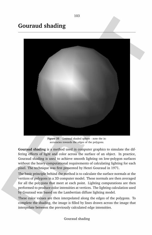
DRAF

T

103

Gouraud shading

Gouraud shading

Figure 35 Gouraud shaded sphere - note the in-accuracies towards the edges of the polygons.

Gouraud shading is a method used in computer graphics to simulate the dif-fering effects of light and color across the surface of an object. In practice,Gouraud shading is used to achieve smooth lighting on low-polygon surfaceswithout the heavy computational requirements of calculating lighting for eachpixel. The technique was first presented by Henri Gouraud in 1971.

The basic principle behind the method is to calculate the surface normals at thevertices of polygons in a 3D computer model. These normals are then averagedfor all the polygons that meet at each point. Lighting computations are thenperformed to produce color intensities at vertices. The lighting calculation usedby Gouraud was based on the Lambertian diffuse lighting model.

These color values are then interpolated along the edges of the polygons. Tocomplete the shading, the image is filled by lines drawn across the image thatinterpolate between the previously calculated edge intensities.

DRAF

T

104

Gouraud shading

Gouraud shading is much less processor intensive than →Phong shading, butdoes not calculate all desirable lighting effects as accurately. For instance, thewhite shiny spot on the surface of an apple (called a specular highlight) ishighly dependent on the normal within that spot. If a model’s vertices are notwithin that spot, their colors are blended across it, making it disappear alto-gether. This problem is made more obvious when the light source is relocated,moving the highlight across a vertex. Using Gouraud shading, the specularhighlight will appear mysteriously and grow in intensity as the light moves to-ward a position of reflection from the observer across the vertex. The desiredresult would be to see the highlight move smoothly rather than fade out and inbetween vertices.

Despite the drawbacks, Gouraud shading is much superior to flat shadingwhich requires significantly less processing than Gouraud, but gives low-polygon models a sharp, faceted look.

Original publications

• H. Gouraud, "Continuous shading of curved surfaces," IEEE Transactions onComputers, 20(6):623–628, 1971.

• H. Gouraud, Computer Display of Curved Surfaces, Doctoral Thesis, Uni-versity of Utah, USA, 1971.

• H. Gouraud, Continuous shading of curved surfaces. In Rosalee Wolfe (ed-itor), Seminal Graphics: Pioneering efforts that shaped the field89, ACMPress, 1998. ISBN 1-58113-052-X.

See also

• →Blinn–Phong shading model

Source: http://en.wikipedia.org/wiki/Gouraud_shading

Principal Authors: Jpbowen, Blueshade, Kocio, Michael Hardy, Mrwojo, Jaxl, Zundark, Poccil, The

Anome

http://www.siggraph.org/publications/seminal-graphics.html89

DRAF

T

105

Graphics pipeline

Graphics pipeline

In 3D computer graphics, the terms graphics pipeline or rendering pipelinemost commonly refer to the current state of the art method of rasterization-based rendering as supported by commodity graphics hardware. The graphicspipeline typically accepts some representation of a 3D scene as an input andresults in a 2D raster image as output.

Stages of the graphics pipeline:

• Modeling transformation• Lighting• Viewing transformation• Projection transformation• Clipping• Scan conversion or rasterization• Texturing or shading• Display

Modeling transformationIn this stage the 3D geometry provided as input is established in what is knownas 3D world-space—a conceptual orientation and arrangement in 3D space.This could include transformations on the local object-space of geometric prim-itives such as translation and rotation.

LightingGeometry in the complete 3D scene is lit according to the defined locationsof light sources and reflectance and other surface properties. Current hard-ware implementations of the graphics pipeline compute lighting only at thevertices of the polygons being rendered. The lighting values between verticesare then interpolated during rasterization. Per-pixel lighting can be done onmodern graphics hardware as a post-rasterization process by means of a frag-ment shader program.

Viewing transformationObjects are transformed from 3D world-space coordinates into a 3D coordinatesystem based on the position and orientation of a virtual camera. This resultsin the original 3D scene as seen from the camera’s point of view, defined inwhat it called eye-space or camera-space.

DRAF

T

106

Graphics pipeline

Projection transformationIn this stage of the graphics pipeline, geometry is transformed from the eye-space of the rendering camera into 2D image-space, mapping the 3D sceneonto a plane as seen from the virtual camera.

Clipping

For more details on this topic, see Clipping (computer graphics).

Geometric primitives that now fall outside of the viewing frustum will not bevisible and are discarded at this stage. Clipping is not necessary to achievea correct image output, but it accelerates the rendering process by eliminat-ing the unneeded rasterization and post-processing on primitives that will notappear anyway.

Scan conversion or rasterizationRasterization is the process by which the 2D image-space representation of thescene is converted into raster format and the correct resulting pixel values aredetermined.

Texturing or shadingAt this stage of the pipeline individual fragments (or pre-pixels) are assigneda color based on values interpolated from the vertices during rasterization orfrom a texture in memory.

DisplayThe final colored pixels can then be displayed on a computer monitor or otherdisplay.

The Graphics Pipeline in HardwareThe rendering pipeline is mapped onto current graphics acceleration hardwaresuch that the input to the graphics card (GPU) is in the form of vertices. Thesevertices then undergo transformation and per-vertex lighting. At this point inmodern GPU pipelines a custom vertex shader program can be used to ma-nipulate the 3D vertices prior to rasterization. Once transformed and lit, thevertices undergo clipping and rasterization resulting in fragments. A secondcustom shader program can then be run on each fragment before the finalpixel values are output to the frame buffer for display.

The graphics pipeline is well suited to the rendering process because it allowsthe GPU to function as a stream processor since all vertices and fragments

DRAF

T

107

Graphics pipeline

can be thought of as independent. This allows all stages of the pipeline tobe used simultaneously for different vertices or fragments as they work theirway through the pipe. In addition to pipelining vertices and fragments, theirindependence allows graphics processors to use parallel processing units toprocess multiple vertices or fragments in a single stage of the pipeline at thesame time.

References

1. ↑ Graphics pipeline. (n.d.). Computer Desktop Encyclopedia. RetrievedDecember 13, 2005, from Answers.com Web site: 90

2. ↑ Raster Graphics and Color91 2004 by Greg Humphreys at the Universityof Virginia

See also

• Rendering• Graphics Processing Unit• Stream Processor• →Shader• NVIDIA• ATI

External links

• MIT OpenCourseWare Computer Graphics, Fall 200392

• Answers.com overview of the graphics pipeline93

• OpenGL94

• DirectX95

Source: http://en.wikipedia.org/wiki/Graphics_pipeline

Principal Authors: Flamurai, Seasage, Sfingram, Piotrus, Hellisp

http://www.answers.com/topic/graphics-pipeline90

http://www.cs.virginia.edu/~gfx/Courses/2004/Intro.Fall.04/handouts/01-raster.pdf91

http://ocw.mit.edu/OcwWeb/Electrical-Engineering-and-Computer-Science/6-837Fall2003/CourseHome92

/index.htmhttp://www.answers.com/topic/graphics-pipeline93

http://www.opengl.org/about/overview.html94

http://www.microsoft.com/windows/directx/default.aspx95

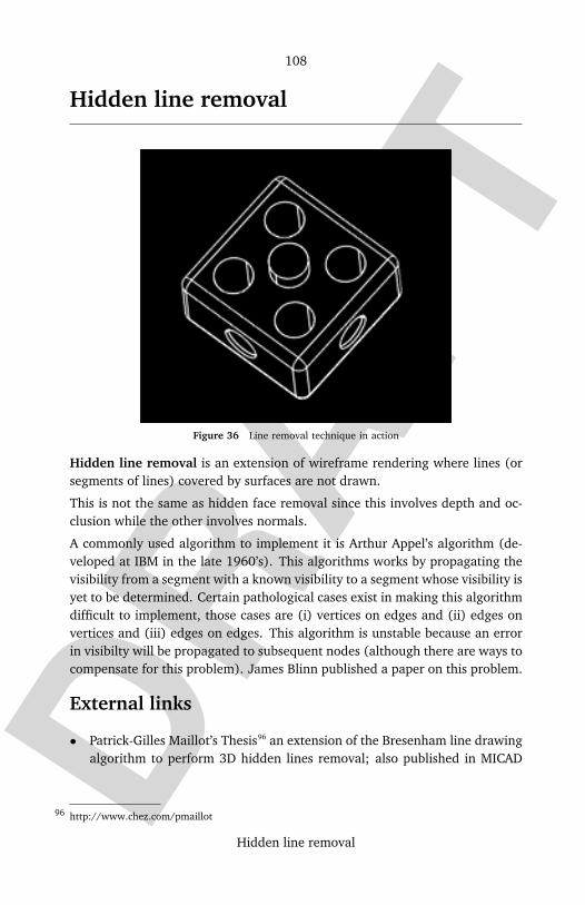
DRAF

T

108

Hidden line removal

Hidden line removal

Figure 36 Line removal technique in action

Hidden line removal is an extension of wireframe rendering where lines (orsegments of lines) covered by surfaces are not drawn.

This is not the same as hidden face removal since this involves depth and oc-clusion while the other involves normals.

A commonly used algorithm to implement it is Arthur Appel’s algorithm (de-veloped at IBM in the late 1960’s). This algorithms works by propagating thevisibility from a segment with a known visibility to a segment whose visibility isyet to be determined. Certain pathological cases exist in making this algorithmdifficult to implement, those cases are (i) vertices on edges and (ii) edges onvertices and (iii) edges on edges. This algorithm is unstable because an errorin visibilty will be propagated to subsequent nodes (although there are ways tocompensate for this problem). James Blinn published a paper on this problem.

External links

• Patrick-Gilles Maillot’s Thesis96 an extension of the Bresenham line drawingalgorithm to perform 3D hidden lines removal; also published in MICAD

http://www.chez.com/pmaillot96

DRAF

T

109

Hidden surface determination

’87 proceedings on CAD/CAM and Computer Graphics, page 591 - ISBN2-86601-084-1.

• Vector Hidden Line Removal97 An article by Walter Heger with a furtherdescription (of the pathelogical cases) and more citations.

Source: http://en.wikipedia.org/wiki/Hidden_line_removal

Principal Authors: MrMambo, Grutness, Qz, RJHall, Oleg Alexandrov


In →3D computer graphics, hidden surface determination is the process usedto determine which surfaces and parts of surfaces are not visible from a cer-tain viewpoint. A hidden surface determination algorithm is a solution to thevisibility problem, which was one of the first major problems in the field of3D computer graphics. The process of hidden surface determination is some-times called hiding, and such an algorithm is sometimes called a hider. Theanalogue for line rendering is hidden line removal.

Hidden surface determination is necessary to render an image correctly, asparts of the image that are not visible should not be drawn. It also speeds uprendering since objects that aren’t visible can be removed from the graphicspipeline.

There are many techniques for hidden surface determination, and the core dif-ferences between most rendering algorithms is how they handle this problem.There are also different stages of hidden surface determination. These stagesinclude:

Backface culling

Since meshes are hollow shells, not solid objects, the back side of somefaces, or polygons, in the mesh will never face the camera. Typically, thereis no reason to draw such faces. This is responsible for the effect often seenin computer and video games in which, if the camera happens to be insidea mesh, rather than seeing the "inside" surfaces of the mesh, it disappearscompletely (all faces are seen from behind, and are culled).

Viewing frustum culling

http://wheger.tripod.com/vhl/vhl.htm97

DRAF

T

110


The viewing frustum is a geometric representation of the volume visibleto the virtual camera. Naturally, objects outside this volume will not bevisible in the final image, so they are discarded. Often, objects lie on theboundary of the viewing frustum. These objects are cut into pieces alongthis boundary in a process called clipping, and the pieces that lie outsidethe frustum are discarded.

Occlusion culling

Occlusion culling is the process of determining which portions of objectsare hidden by other objects from a given viewpoint. This is one of thefundamental problems in computer graphics, and many different occlusionculling algorithms have been developed. The simplest is painter’s algo-rithm, in which polygons are sorted, then drawn back to front. The mostcommon in real-time computer graphics is z-buffering, in which the depthvalue at each pixel is stored as each polygon is rendered. The pixel is onlyoverwritten if the depth value of the current point is less than the depth val-ue stored in the z-buffer. Both of these methods operate on polygon meshes.

Contribution culling

Often, objects are so far away that they do not contribute significantly tothe final image. These objects are thrown away if their screen projection istoo small.

Though hidden surface determination is most often used to determine what isvisible in the final image, it is also has other applications, such as determiningwhich parts of objects are in shadow.

Visible surface determinationSometimes the majority of surfaces is invisible, so why ever touch them? Thisapproach is opposite to hidden surface removal and used in:

• Ray tracer : →Ray tracing, which can also operate on parametric geometry,attempts to model the path of light rays into a viewpoint by tracing raysfrom the viewpoint into the scene. The first object the ray intersects isrendered, as it naturally is the object visible to the camera. Additional datastructures used to solve this sorting problem include bsp trees and octrees.

• Portal rendering• some Heightfield renderers work this way. Google Earth certainly does not

process the whole earth for every frame.

DRAF

T

111

High dynamic range imaging

Source: http://en.wikipedia.org/wiki/Hidden_surface_determination

Principal Authors: Flamurai, Fredrik, B4hand, Connelly, Arnero


Figure 37 Tone Mapped HDRI example showing stained glass windows in south alcove of OldSaint Paul’s, Wellington, New Zealand.

In computer graphics and cinematography, high dynamic range imaging(HDRI for short) is a set of techniques that allow a far greater dynamic rangeof exposures than normal digital imaging techniques. The intention is to accu-rately represent the wide range of intensity levels found in real scenes, rangingfrom direct sunlight to the deepest shadows.

This provides the opportunity to shoot a scene and have total control of thefinal imaging from the beginning to the end of the photography project. Anexample would be that it provides the possibility to re-expose. One can captureas wide a range of information as possible on location and choose what iswanted later.

Gregory Ward is widely considered to be the founder of the file format for highdynamic range imaging. The use of high dynamic range imaging in computergraphics has been pioneered by Paul Debevec. He is considered to be the first

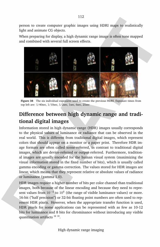
DRAF

T

112


person to create computer graphic images using HDRI maps to realisticallylight and animate CG objects.

When preparing for display, a high dynamic range image is often tone mappedand combined with several full screen effects.

Figure 38 The six individual exposures used to create the previous HDRI. Exposure times fromtop left are: 1/40sec, 1/10sec, 1/2sec, 1sec, 6sec, 25sec

Difference between high dynamic range and tradi-tional digital imagesInformation stored in high dynamic range (HDR) images usually correspondsto the physical values of luminance or radiance that can be observed in thereal world. This is different from traditional digital images, which representcolors that should appear on a monitor or a paper print. Therefore HDR im-age formats are often called scene-referred, in contrast to traditional digitalimages, which are device-referred or output-referred. Furthermore, tradition-al images are usually encoded for the human visual system (maximizing thevisual information stored in the fixed number of bits), which is usually calledgamma encoding or gamma correction. The values stored for HDR images arelinear, which means that they represent relative or absolute values of radianceor luminance (gamma 1.0).

HDR images require a higher number of bits per color channel than traditionalimages, both because of the linear encoding and because they need to repre-sent values from 10−4 to 108 (the range of visible luminance values) or more.16-bit ("half precision") or 32-bit floating point numbers are often used to rep-resent HDR pixels. However, when the appropriate transfer function is used,HDR pixels for some applications can be represented with as few as 10-12bits for luminance and 8 bits for chrominance without introducing any visiblequantization artifacts 98 99.

DRAF

T

113


Example HDR Images

Figure 39 Nave in Old Saint Paul’s,Wellington, NewZealand. Eight exposures ranging from 1/20th of a secondto 30 seconds

See also

• →High dynamic range rendering (rendering virtual scenes using high dy-namic range lighting calculation, notably in computer games)

• OpenEXR• Radiance file format• Logluv TIFF file format• CinePaint image editor• Pixel image editor• Panoscan

http://www.anyhere.com/gward/hdrenc/hdr_encodings.html98

http://www.mpi-sb.mpg.de/resources/hdrvideo/99

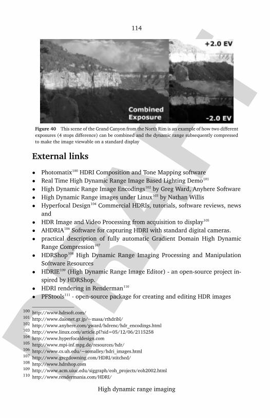
DRAF

T

114


Figure 40 This scene of the Grand Canyon from the North Rim is an example of how two differentexposures (4 stops difference) can be combined and the dynamic range subsequently compressedto make the image viewable on a standard display

External links

• Photomatix100 HDRI Composition and Tone Mapping software• Real Time High Dynamic Range Image Based Lighting Demo101

• High Dynamic Range Image Encodings102 by Greg Ward, Anyhere Software• High Dynamic Range images under Linux103 by Nathan Willis• Hyperfocal Design104 Commercial HDRIs, tutorials, software reviews, news

and• HDR Image and Video Processing from acquisition to display105

• AHDRIA106 Software for capturing HDRI with standard digital cameras.• practical description of fully automatic Gradient Domain High Dynamic

Range Compression107

• HDRShop108 High Dynamic Range Imaging Processing and ManipulationSoftware Resources

• HDRIE109 (High Dynamic Range Image Editor) - an open-source project in-spired by HDRShop.

• HDRI rendering in Renderman110

• PFStools111 - open-source package for creating and editing HDR images

http://www.hdrsoft.com/100

http://www.daionet.gr.jp/~masa/rthdribl/101

http://www.anyhere.com/gward/hdrenc/hdr_encodings.html102

http://www.linux.com/article.pl?sid=05/12/06/2115258103

http://www.hyperfocaldesign.com104

http://www.mpi-inf.mpg.de/resources/hdr/105

http://www.cs.uh.edu/~somalley/hdri_images.html106

http://www.gregdowning.com/HDRI/stitched/107

http://www.hdrshop.com108

http://www.acm.uiuc.edu/siggraph/eoh_projects/eoh2002.html109

http://www.rendermania.com/HDRI/110

DRAF

T

115

High dynamic range rendering

Photography:

• High Dynamic Range (HDR) in Photography112 - Implementation in Photo-shop CS2

HDR displays:

• http://www.brightsidetech.com/ High Dynamic Range Displays• Technical information on HDR displays113

Studio rendering:

• http://www.hdri-studio.com Commercial HDR maps derived from studiolighting setups

• http://www.sachform.com Commercial HDR panoramas and viewer.• PixelBox Academy HDRI Tutorial114 HDRI in PRMan using Image Based Il-

lumination

On Rendering, but need descriptions, should be deleted otherwise:

Source: http://en.wikipedia.org/wiki/High_dynamic_range_imaging

Principal Authors: Imroy, Tnikkel, Rafm, Deanpemberton, Diliff, Noclip, Toytoy


High dynamic range rendering (HDRR or HDR Rendering) or less common-ly, high dynamic range lighting (HDR Lighting), is the rendering of 3D com-puter graphics scenes by using lighting calculations done in a high dynamicrange. Specifically it refers to the new lighting model used to illuminate 3Dworlds. Video games and computer generated movies greatly benefit from thisas it creates far more realistic scenes than with conventional lighting models.

http://www.mpi-inf.mpg.de/resources/pfstools/111

http://www.cambridgeincolour.com/tutorials/high-dynamic-range.htm112

http://www.cs.ubc.ca/~heidrich/Projects/HDRDisplay113

http://pbacademy.com.sapo.pt/tutorials/renderman/hdri.htm114

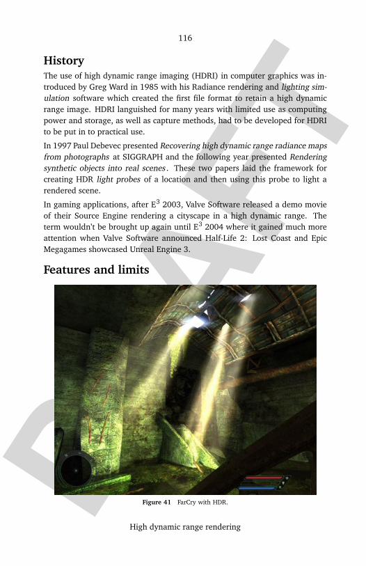
DRAF

T

116


HistoryThe use of high dynamic range imaging (HDRI) in computer graphics was in-troduced by Greg Ward in 1985 with his Radiance rendering and lighting sim-ulation software which created the first file format to retain a high dynamicrange image. HDRI languished for many years with limited use as computingpower and storage, as well as capture methods, had to be developed for HDRIto be put in to practical use.

In 1997 Paul Debevec presented Recovering high dynamic range radiance mapsfrom photographs at SIGGRAPH and the following year presented Renderingsynthetic objects into real scenes . These two papers laid the framework forcreating HDR light probes of a location and then using this probe to light arendered scene.

In gaming applications, after E3 2003, Valve Software released a demo movieof their Source Engine rendering a cityscape in a high dynamic range. Theterm wouldn’t be brought up again until E3 2004 where it gained much moreattention when Valve Software announced Half-Life 2: Lost Coast and EpicMegagames showcased Unreal Engine 3.

Features and limits

Figure 41 FarCry with HDR.

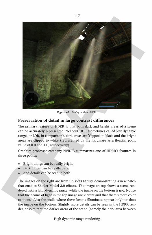
DRAF

T

117


Figure 42 FarCry without HDR.

Preservation of detail in large contrast differencesThe primary feature of HDRR is that both dark and bright areas of a scenecan be accurately represented. Without HDR (sometimes called low dynamicrange, or LDR, in comparison), dark areas are ’clipped’ to black and the brightareas are clipped to white (represented by the hardware as a floating pointvalue of 0.0 and 1.0, respectively).

Graphics processor company NVIDIA summarizes one of HDRR’s features inthree points:

• Bright things can be really bright• Dark things can be really dark• And details can be seen in both

The images on the right are from Ubisoft’s FarCry, demonstrating a new patchthat enables Shader Model 3.0 effects. The image on top shows a scene ren-dered with a high dynamic range, while the image on the bottom is not. Noticethat the beams of light in the top image are vibrant and that there’s more colorto them. Also the walls where these beams illuminate appear brighter thanthe image on the bottom. Slightly more details can be seen in the HDRR ren-der, despite that the darker areas of the scene (namely the dark area between

DRAF

T

118


the two beams) have about the same amount of visibility in both pictures. Inregards to color vibrance, the scene without HDR appears dull.

Accurate reflection of light

Figure 43 From Half-Life 2: Lost Coast, a comparison image between the same scene renderedwith HDRR and without HDRR.

Without HDRR, the sun and most lights are clipped to 100% (1.0 in the frame-buffer). When this light is reflected the result must then be less than or equalto 1.0, since the reflected value is calculated by multiplying the original valueby the surface’s reflectiveness, usually in the range [0, 1]. This makes the lightsappear dull. Using HDR the light produced by the sun and other lights can berepresented with appropriately high values, exceeding the 1.0 clamping limitin the frame buffer, with the sun possibly being stored as 60000. When thelight from them is reflected it will remain relatively high (even for very poorreflectors), which will be clipped to white or properly tonemapped when ren-dered. Looking at the example picture above, from Valve’s Half-Life 2: LostCoast, you can see these reflection differences upon the water and the sand.

An exampleImagine a dark room lit with moonlight, with a desk against the wall, a comput-er monitor on that desk, and a poster on the wall directly behind the monitor.If the scene was rendered in 3D using either 8-bit, 16-bit, or 32-bit lightingprecision, there would be very little difference due to the low dynamic rangeinherent in the scene. Now if the monitor is displaying this web page, the dy-namic range would be high. Human eyes could depict the detail on both theposter and monitor simultaneously better than say a digital camera could, be-cause the digital camera can only "see" in a 256:1 contrast ratio of perception(assuming a linear response curve, which is the case for most CCD-based tech-nology), whereas human eyes can perceive a much higher contrast ratio. This

DRAF

T

119


would mean that the digital camera would have to capture the scene with abit of bias between brightening the scene or darkening the scene by adjustingits exposure. If the scene was brightened, the text upon the monitor would bewashed out in order for the poster to be seen. If the scene was darkened, thedetail on the poster would be lost in favor upon capturing the text displayedon the monitor.

If this scene was rendered with HDR rendering, the detail on both the monitorand the poster would be preserved, without placing bias on brightening ordarkening the scene.

LimitationsThe human eye supports its high dynamic range in part through better bright-ness resolution than what can be done with 8 bits, but it also needs the iristo move its range of sensivity from nearly pitch-black to a white wall in directsunlight at the same time and computer displays can’t do either.

A natural scene exposed in the sunlight can display a contrast of about50,000:1. Negative black and white film can capture a dynamic range of about4096:1 (12 stops) maximum, while color slide film reach can typically cap-ture a dynamic range of 64:1 (6 stops). Printing has the same problems asdisplaying on LDR monitors as color paper only has about 64:1 (6 stops).

On average, most computer monitors have a specified contrast ratio between500:1 and 1000:1, sometimes 1500:1. Current plasma displays are specifiedat a 10,000:1 contrast ratio (most are 50% lower). However, the contrast ofcommercial displays is measured as the ratio of a full white screen to a fullblack screen in a completely dark room. The simultaneous contrast of realcontent under normal viewing conditions is significantly lower.

One of the few monitors that can display in true HDR is the BrightSideTechnologies115 HDR monitor, which has a simultaneous contrast ratio ofaround 200,000:1 for a brightness of 3000 cd.m-2, measured on a checker-board image. In fact this higher contrast is equivalent to a ANSI9 contrastof 60,000:1, or about 60 times higher that the one of a TFT screen (about1000:1). The brightness is 10 times higher that the one of the most CRT orTFT. But such display should only be useful if it needs to operate in a pitch-black room and in two seconds under bright lightning, and the eye should beable to see a full dynamic range on the display in both situations.

This means that HDR rendering systems have to map the full dynamic rangeto what the eye would see in the rendered situation. This tone mapping isdone relative to what the virtual scene camera sees, combined with several full

http://www.brightsidetech.com/115

DRAF

T

120


screen effects, e.g. to simulate dust in the air which is lit by direct sunlight ina dark cavern.

There is currently two graphical effects used to combat these limitations, tonemapping and light blooming, which are often used together.

However, due to the stressing nature of HDRR, it’s not recommended that fullscreen anti-aliasing (FSAA) be enabled while HDRR is enabled at the sametime on current hardware, as this will cause a severe performance drop. Manygames that support HDRR will only allow FSAA or HDRR. However somegames which use a simpler HDR rendering model will allow FSAA at the sametime.

Tone mapping

Figure 44 A screenshot of Day of Defeat: Source. While looking into a dark interior from theoutside, it appears dark.

The limitations of display devices (whose gamuts are very limited comparedto a gamut which supports HDR colors) prevent colors in HDR from beingdisplayed properly. Tone mapping attempts to solve the problem of displayingHDR colors on a LDR display device by mapping colors in a HDR image to LDR.Many different tone mapping operators exist, and vary wildly in complexity

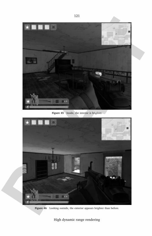
DRAF

T

121


Figure 45 Inside, the interior is brighter.

Figure 46 Looking outside, the exterior appears brighter than before.

DRAF

T

122


Figure 47 But the exterior’s brightness normalizes as one goes outside.

and visual results. Some tone mapping algorithms are also time dependant,as seen in the above images, in an attempt to approximate a human eye’s irisregulation of light entering the eye.

Light Bloom

Main article: →Bloom (shader effect)

Light blooming "spreads" out a light source. For example, a bright light in thebackground will appear to bleed over onto objects in the foreground. This ef-fect is achieved by multiplying the image of the screen (lighten lighter areasand darken darker areas,) blurring the image, and drawing it over top of theoriginal image. If there’s a light source that is "brighter" than what the moni-tor can show, light blooming helps to create an illusion that makes the objectappear brighter than it is, but at the cost of softening the scene. A commonmisconception is that a game that uses a bloom filter uses HDR. This is untrue,however, as blooming is often used alongside HDR, but is not a component ofHDR.

The reason blooming is used alongside HDR is that when a saturated LDRimage is blurred, the result is equivalent to blurring an image with lots of white

DRAF

T

123


areas, simply because values above 1.0 aren’t preserved, so bright areas bur togradients in the range of 1.0 -> 0.0. The result is simply a linear white to blackgradient, regardless of the original color of the bright part. HDR, on the otherhand, preserves colors above 1.0, so the blur result in a gradient between thesaturated value that slowly becomes less and less saturated. A bright blue lightmay appear white at its center, but with HDR it retains the blue color in a haloaround it when the image is blurred.

Applications in computer entertainmentCurrently HDRR has been prevalent in games. Though these games are most-ly for the PC, it is also possible to render scenes in a high dynamic range inMicrosoft’s Xbox 360, Sony’s PlayStation 3, and Nintendo’s Wii. It has alsobeen simulated on the PlayStation 2, GameCube, and Xbox. In desktop pub-lishing and gaming, colour values are often processed several times over. Asthis includes multiplication and division it is useful to have the extended accu-racy and range of 16 bit integer or 16 bit floating point format. This is usefulirrespective of the abovementioned limitations in some hardware.

The development of HDRR into real time rendering mostly came from Mi-crosoft’s DirectX API.

DirectX’s role in HDRR developmentComplex shader effects began its days back with the release of Shader Model1.0 with DirectX 8. Shader Model 1.0 illuminated 3D worlds with what is nowcalled standard lighting. However, standard lighting had two problems:

1. Lighting precision was confined to 8 bit integers, which limited the contrastratio to 256:1. Using the HVS color model, the value (V), or brightness ofa color has a range of 0 - 255. This means the brightest white ( a value of255 ) is only 256 times brighter than the darkest black ( a value of 0 ).

2. Lighting calculations were integer based, which didn’t offer much accuracybecause the real world is not confined to whole numbers 116.

Before HDRR was fully developed and implemented, games would fake theillusion of HDR by using light blooming and sometimes using an option called"Enhanced Contrast Settings" (Need For Speed Underground 2 had this as anoption, while Metal Gear Solid 3 had it on at all times).

On December 24, 2002, Microsoft released a new version of DirectX. DirectX9.0 introduced Shader Model 2.0 which offered one of the necessary compo-nents to enable rendering of high dynamic range rendering, lighting precision

http://download.nvidia.com/developer/presentations/2004/6800_Leagues/6800_Leagues_HDR.pdf116

DRAF

T

124


was not limited to just 8-bits. Although 8-bits was minimum in applications,programmers could choose up to a maximum of 24-bits for lighting precision.However, all calculations were still integer based. One of the first graphicscards to take advantage of DirectX 9.0 was Ati’s Radeon 9700, though the ef-fect wasn’t programmed into games for years to come. On August 23, 2003,Microsoft updated DirectX to DirectX 9.0b, which enabled Pixel Shader 2.x(Extended) profile for ATI’s Radeon X series and NVIDIA’s GeForce FX series ofgraphics processing units.

On August 9, 2004, Microsoft updated DirectX once more to DirectX 9.0c.This also exposed the Shader Model 3.0 profile for high level shader language(HLSL). Shader Model 3.0’s lighting precision, according to Dr. Sim DietrichJr., has a minimum of 32-bits as opposed to 2.0’s 8-bit minimum. Also all light-ing precision calculations are now floating-point based. NVIDIA states thatcontrast ratios using Shader Model 3.0 can be as high as 65535:1 using 32-bitlighting precision. At first, HDRR was only capable on video cards capable ofShader Model 3.0 effects, but software developers soon added compatibilityfor Shader Model 2.0. The difference between an HDRR scene rendered inShader Model 3.0 or 2.0 is negligible at this point. As a side note, when re-ferred as Shader Model 3.0 HDR, the HDRR is really done by FP16 blending.FP16 blending is not part of Shader Model 3.0, but supported only by cardsalso capable of Shader Model 3.0, excluding the GeForce 6200 models as theylack the capabilities. FP16 blending is used as a faster way to render HDR invideo games.

It is unsure what HDR upgrades will be available from Shader Model 4.0 (tobe released with DirectX 10).

Graphics cards which support HDRRThis is a list of Graphics cards that may or can support HDRR. It is implied thatbecause the minimum requirement for HDR rendering is Shader Model 2.0 (orin this case DirectX 9), any graphics card that supports Shader Model 2.0 cando HDR rendering. However, HDRR may greatly impact the performance ofthe software using it, refer to your software’s recommended specifications inorder to run with acceptable performance.

Graphics cards designed for gamesShader Model 2 Compliant (Includes versions 2.0, 2.0a and 2.0b)

From ATI R300 series: 9500, 9500 Pro, 9550, 9550 SE, 9600, 9600 SE, 9600 AIW, 9600Pro, 9600 XT, 9650, 9700, 9700 AIW, 9700 Pro, 9800, 9800 SE, 9800 AIW,9800 Pro, 9800XT, X300, X300 SE, X550, X600 AIW, X600 Pro, X600 XT R420series: X700, X700 Pro, X700 XT, X800, X800SE, X800 GT, X800 GTO, X800Pro, X800 AIW, X800 XL, X800 XT, X800 XTPE, X850 Pro, X850 XT, X850XTPE

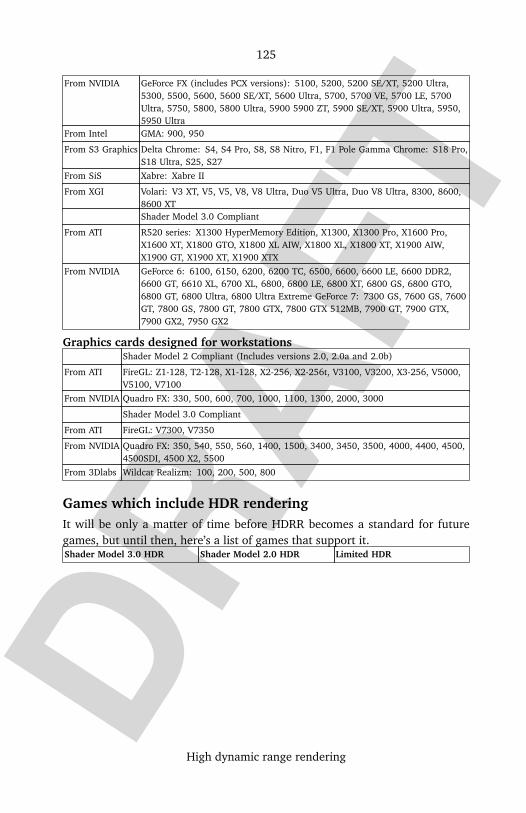
DRAF

T

125


From NVIDIA GeForce FX (includes PCX versions): 5100, 5200, 5200 SE/XT, 5200 Ultra,5300, 5500, 5600, 5600 SE/XT, 5600 Ultra, 5700, 5700 VE, 5700 LE, 5700Ultra, 5750, 5800, 5800 Ultra, 5900 5900 ZT, 5900 SE/XT, 5900 Ultra, 5950,5950 Ultra

From Intel GMA: 900, 950

From S3 Graphics Delta Chrome: S4, S4 Pro, S8, S8 Nitro, F1, F1 Pole Gamma Chrome: S18 Pro,S18 Ultra, S25, S27

From SiS Xabre: Xabre II

From XGI Volari: V3 XT, V5, V5, V8, V8 Ultra, Duo V5 Ultra, Duo V8 Ultra, 8300, 8600,8600 XTShader Model 3.0 Compliant

From ATI R520 series: X1300 HyperMemory Edition, X1300, X1300 Pro, X1600 Pro,X1600 XT, X1800 GTO, X1800 XL AIW, X1800 XL, X1800 XT, X1900 AIW,X1900 GT, X1900 XT, X1900 XTX

From NVIDIA GeForce 6: 6100, 6150, 6200, 6200 TC, 6500, 6600, 6600 LE, 6600 DDR2,6600 GT, 6610 XL, 6700 XL, 6800, 6800 LE, 6800 XT, 6800 GS, 6800 GTO,6800 GT, 6800 Ultra, 6800 Ultra Extreme GeForce 7: 7300 GS, 7600 GS, 7600GT, 7800 GS, 7800 GT, 7800 GTX, 7800 GTX 512MB, 7900 GT, 7900 GTX,7900 GX2, 7950 GX2

Graphics cards designed for workstationsShader Model 2 Compliant (Includes versions 2.0, 2.0a and 2.0b)

From ATI FireGL: Z1-128, T2-128, X1-128, X2-256, X2-256t, V3100, V3200, X3-256, V5000,V5100, V7100

From NVIDIA Quadro FX: 330, 500, 600, 700, 1000, 1100, 1300, 2000, 3000

Shader Model 3.0 Compliant

From ATI FireGL: V7300, V7350

From NVIDIA Quadro FX: 350, 540, 550, 560, 1400, 1500, 3400, 3450, 3500, 4000, 4400, 4500,4500SDI, 4500 X2, 5500

From 3Dlabs Wildcat Realizm: 100, 200, 500, 800

Games which include HDR renderingIt will be only a matter of time before HDRR becomes a standard for futuregames, but until then, here’s a list of games that support it.Shader Model 3.0 HDR Shader Model 2.0 HDR Limited HDR

DRAF

T

126


• Act of War: High Treason• Age of Empires III• Bet on Soldier• Bioshock• Brothers In Arms: Hell’s

Highway• Crysis• Duke Nukem Forever• Far Cry

• (with patch 1.3installed)

• Far Cry Instincts: Predator

Romani in Spatiu

• Gears of War• Huxley• Juiced

• (PC version only)• Kameo: Elements of Power• The Lord of the Rings: The

Battle for Middle-earth• The Lord of the Rings: The

Battle for Middle-earth II• Lineage II

• (with Chronicle 4updated)

• Project Gotham Racing 3• Project Offset• Perfect Dark Zero• Serious Sam II• Stranglehold• The Elder Scrolls IV:

Oblivion• TimeShift• Tom Clancy’s Ghost Recon:

Advanced Warfighter• Tom Clancy’s Splinter Cell:

Chaos Theory• (PC version only)

• Tom Clancy’s Splinter Cell:Double Agent• (PC and Xbox 360

version only)• Tomb Raider: Legend

• (PC and Xbox 360version only)

• Unreal Tournament 2007• Vanguard: Saga of Heroes

• Act of War: High Treason• Bioshock• Brothers In Arms: Hell’s

Highway• Brothers in Arms: Earned in

Blood• Brothers in Arms: Road to

Hill 30• Call of Duty 2• Counter-Strike: Source

• (Limited to certainmaps)

• Crysis• Day of Defeat: Source• Far Cry

• (SM 2.0 HDR patchsoon)

• Gears of War• Half-Life 2: Episode One• Half-Life 2: Lost Coast• Huxley• Red Orchestra: Ostfront

41-45• Stranglehold• Tom Clancy’s Splinter Cell:

Chaos Theory• (PC version only with

patch 1.4 installed)• Tom Clancy’s Splinter Cell:

Double Agent• (PC version only)

• Unreal Tournament 2007• Vanguard: Saga of Heroes

• Deus Ex: Invisible War• Need for Speed:

Underground 2• Shadow of the Colossus• Operation Flashpoint: Elite• Pariah• Metal Gear Solid 3: Snake

Eater• Spartan: Total Warrior• SWAT 4• SWAT 4: The Stetchkov

Syndicate• Thief: Deadly Shadows• Tribes Vengeance• Unreal Championship 2• WarPath

DRAF

T

127


Links

External links and sources

• NVIDIA’s HDRR technical summary117 (PDF)• Microsoft’s technical brief on SM3.0 in comparison with SM2.0118

• High Dynamic Range Rendering in Photoshop CS2119 - Applications to digi-tal photography

• Horror Blog120

• Tom’s Hardware: New Graphic Card Features of 2006121

• The Contrast Ratio Number Game122

• List of GPU’s compiled by Chris Hare123

• techPowerUp! GPU Database124

Software developer websites

• Source Engine Licensing125 (see Source Engine for more)• Half-Life 2126

• Unreal Engine 3127

• Emergent’s Gamebryo128

• CryEngine129

• FarCry130

Real-time HDR rendering

• Real time HDR demo for PCs131

• 3D Engine with HDR previewing132

• Unigine with HDR Rendering Demos133

http://download.nvidia.com/developer/presentations/2004/6800_Leagues/6800_Leagues_HDR.pdf117

http://www.microsoft.com/whdc/winhec/partners/shadermodel30_NVIDIA.mspx118

http://www.cambridgeincolour.com/tutorials/high-dynamic-range.htm119

http://www.codinghorror.com/blog/archives/000324.html|Coding120

http://www.tomshardware.com/2006/01/13/new_3d_graphics_card_features_in_2006/121

http://www.practical-home-theater-guide.com/contrast-ratio.html122

http://users.erols.com/chare/video.htm123

http://www.techpowerup.com/gpudb/124

http://www.valvesoftware.com/sourcelicense/125

http://www.half-life2.com/126

http://www.unrealtechnology.com/html/technology/ue30.shtml127

http://www.emergent.net128

http://www.crytek.com129

http://www.farcry-thegame.com130

http://www.daionet.gr.jp/~masa/rthdribl/131

http://powerrender.com/132

http://unigine.com/133

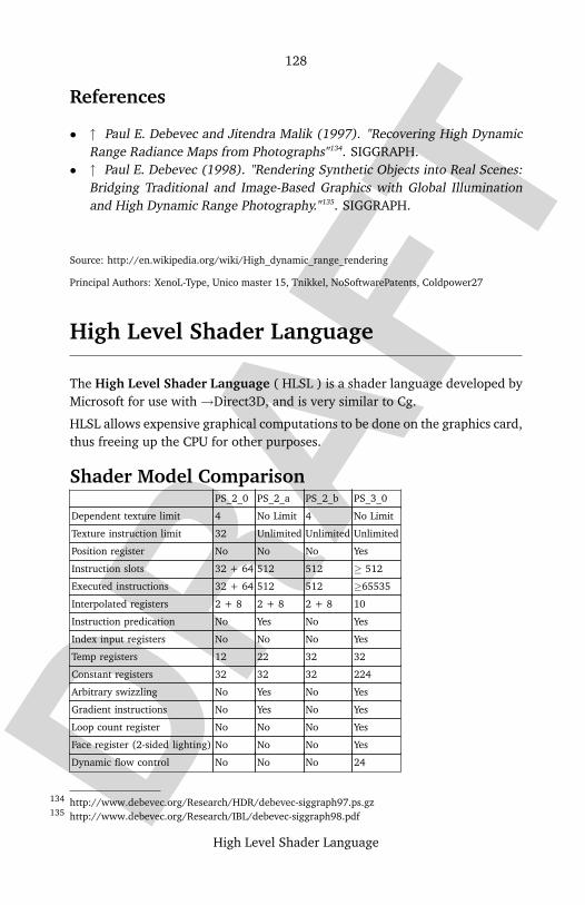
DRAF

T

128

High Level Shader Language

References

• ↑ Paul E. Debevec and Jitendra Malik (1997). "Recovering High DynamicRange Radiance Maps from Photographs"134. SIGGRAPH.

• ↑ Paul E. Debevec (1998). "Rendering Synthetic Objects into Real Scenes:Bridging Traditional and Image-Based Graphics with Global Illuminationand High Dynamic Range Photography."135. SIGGRAPH.

Source: http://en.wikipedia.org/wiki/High_dynamic_range_rendering

Principal Authors: XenoL-Type, Unico master 15, Tnikkel, NoSoftwarePatents, Coldpower27

High Level Shader Language

The High Level Shader Language ( HLSL ) is a shader language developed byMicrosoft for use with →Direct3D, and is very similar to Cg.

HLSL allows expensive graphical computations to be done on the graphics card,thus freeing up the CPU for other purposes.

Shader Model ComparisonPS_2_0 PS_2_a PS_2_b PS_3_0

Dependent texture limit 4 No Limit 4 No Limit

Texture instruction limit 32 Unlimited Unlimited Unlimited

Position register No No No Yes

Instruction slots 32 + 64 512 512 ≥ 512

Executed instructions 32 + 64 512 512 ≥65535

Interpolated registers 2 + 8 2 + 8 2 + 8 10

Instruction predication No Yes No Yes

Index input registers No No No Yes

Temp registers 12 22 32 32

Constant registers 32 32 32 224

Arbitrary swizzling No Yes No Yes

Gradient instructions No Yes No Yes

Loop count register No No No Yes

Face register (2-sided lighting) No No No Yes

Dynamic flow control No No No 24

http://www.debevec.org/Research/HDR/debevec-siggraph97.ps.gz134

http://www.debevec.org/Research/IBL/debevec-siggraph98.pdf135

DRAF

T

129

Humanoid Animation

• PS_2_0 = DirectX 9.0 original Shader Model 2 specification.• PS_2_a = NVIDIA GeForce FX-optimized model, DirectX 9.0a.• PS_2_b = ATI Radeon X700, X800, X850 shader model, DirectX 9.0b.• PS_3_0 = Shader Model 3.

External links

• HLSL Introduction136

• Shader Model Comparison at Beyond3D137

Source: http://en.wikipedia.org/wiki/High_Level_Shader_Language

Principal Authors: Swaaye, Nabla, TheSock, Unixxx, Soumyasch

Humanoid Animation

Humanoid Animation (H-Anim) is an approved ISO standard for humanoidmodeling and animation. H-Anim defines a specification for defining inter-changeable human figures so that those characters can be used across a varietyof 3D games and simulation environments.

External links

• Humanoid Animation Working Group138

• Web3D Consortium139

• X3D Specification140

• ISO/IEC 19774:2006 Humanoid Animation (H-Anim)141

Source: http://en.wikipedia.org/wiki/Humanoid_Animation

Principal Authors: Mditto, X42bn6, Perfecto

http://www.neatware.com/lbstudio/web/hlsl.html136

http://www.beyond3d.com/reviews/ati/r420_x800/index.php?p=8137

http://www.h-anim.org138

http://www.web3d.org139

http://www.web3d.org/x3d/specifications140

http://www.iso.org/iso/en/CatalogueDetailPage.CatalogueDetail?CSNUMBER=33912141

DRAF

T

130

Image based lighting

Image based lighting

Image based lighting is a global illumination method used in 3D photo re-alistic rendering in which an image is used to light the scene in conjunctionwith tradional light models. Image based lighting, or IBL, is generally HDR,although LDR can be used, and provides a larger range of light sampling thencan be obtained through traditional light models. LDR, low dynamic range,works similar to HDR, but offers a much smaller range of lighting information.

Almost every modern renderer offers some type of image based lighting, how-ever the terminology used in their application might be slightly different.

Image based lighting is also starting to show up in game technology since mostgame consoles and computers have such an immense amount of processingpower today.

References

• Tutorial142

See also

• →Ambient occlusion• Final gathering• →Global illumination• →High dynamic range imaging• Light transport theory

Source: http://en.wikipedia.org/wiki/Image_based_lighting

http://www.debevec.org/CGAIBL2/ibl-tutorial-cga2002.pdf142

DRAF

T

131

Inverse kinematic animation

Image plane

In →3D computer graphics, the image plane is that plane in the world whichis identified with the plane of the monitor. If one makes the analogy of taking aphotograph to rendering a 3D image, the surface of the film is the image plane.In this case, the viewing transformation is a projection that maps the worldonto the image plane. A rectangular region of this plane, called the viewingwindow or viewport, maps to the monitor. This establishes the mapping be-tween pixels on the monitor and points (or rather, rays) in the 3D world.

Source: http://en.wikipedia.org/wiki/Image_plane

Principal Authors: TheParanoidOne, RJHall, CesarB, Reedbeta

Inverse kinematic animation

Inverse kinematic animation (IKA) refers to a process utilized in 3D comput-er graphic animation, to calculate the required articulation of a series of limbsor joints, such that the end of the limb ends up in a particular location. Incontrast to forward kinematic animation, where each movement for each com-ponent must be planned, only the starting and ending locations of the limb arenecessary.

For example, when one wants to reach for a door handle, their brain mustmake the necessary calculations to position his limbs and torso such that thehand locates near the door. The main objective is to move the hand but themany complex articulations of several joints must occur to get the hand tothe desired location. Similarly with many technological applications, inversekinematic mathematical calculations must be performed to articulate limbs inthe correct ways to meet desired goals.

One example where inverse kinematic calculations are often essential isrobotics, where an operator wants to position a tool using a robot arm butcertainly doesn’t want to manipulate each robot joint individually. Other ap-plications include computer animation where animators may want to operatea computer generated character, but find it impossibly difficult to animate in-dividual joints. The solution is to model the virtual joints of the puppet andallow the animator to move the hands feet and torso, and the computer auto-matically generates the required limb positions to accomplish this using inversekinematics.

DRAF

T

132

Inverse kinematics

Key to the successful implementation of inverse kinematics is animation withinconstraints: computer characters’ limbs must behave within reasonable anthro-pomorphic limits. Similarly, robotic devices have physical constraints such asthe environment they operate in, the limitations of the articulations their jointsare capable of, and the finite physical loads and speeds at which they are ableto operate.

See also: →Inverse kinematics

Source: http://en.wikipedia.org/wiki/Inverse_kinematic_animation

Principal Authors: Stevertigo, FrenchIsAwesome, Diberri, Stefan, Bryan Derksen

Inverse kinematics

Inverse kinematics is the process of determining the parameters of a jointedflexible object in order to achieve a desired pose. For example, with a 3Dmodel of a human body, what are the required wrist and elbow angles to movethe hand from a resting position to a waving position? This question is vitalin robotics, where manipulator arms are commanded in terms of joint angles.Inverse kinematics are also relevant to game programming and→3D modeling,though its importance there has decreased with the rise of use of large librariesof motion capture data.

An articulated figure consists of a set of rigid segments connected with joints.Varying angles of the joints yields an indefinite number of configurations. Thesolution to the forward kinematics problem, given these angles, is the poseof the figure. The more difficult solution to the inverse kinematics problemis to find the joint angles given the desired configuration of the figure (i.e.,end-effector). In the general case there is no analytic solution for the inversekinematics problem. However, inverse kinematics may be solved via nonlin-ear programming techniques. Certain special kinematic chains—those with aspherical wrist—permit kinematic decoupling. This treats the end-effector’sorientation and position independently and permits an efficient closed-formsolution.

For animators, the inverse kinematics problem is of great importance. Theseartists find it far simpler to express spatial appearance rather than joint angles.Applications of inverse kinematic algorithms include interactive manipulation,animation control and collision avoidance.

See also: →Inverse kinematic animation

DRAF

T

133

Irregular Z-buffer

External links

• Inverse Kinematics algorithms143

• Robot Inverse Kinematics144

• HowStuffWorks.com article How do the characters in video games move sofluidly? 145 with an explanation of inverse kinematics

• 3D Theory Kinematics146

• Protein Inverse Kinematics147

Source: http://en.wikipedia.org/wiki/Inverse_kinematics

Principal Authors: Frecklefoot, GTubio, K.Nevelsteen, Charles Matthews, Dvavasour

Irregular Z-buffer

The irregular Z-buffer is an algorithm designed to solve the visibility problemin real-time 3-d computer graphics. It is related to the classical Z-buffer in thatit maintains a depth value for each image sample and uses these to determinewhich geometric elements of a scene are visible. The key difference, however,between the classical Z-buffer and the irregular Z-buffer is that the latter allowsarbitrary placement of image samples in the image plane, whereas the formerrequires samples to be arranged in a regular grid (See Figure 1).

These depth samples are explicitly stored in a two-dimensional spatial datastructure. During rasterization, triangles are projected onto the image plane asusual, and the data structure is queried to determine which samples overlapeach projected triangle. Finally, for each overlapping sample, the standardZ-compare and (conditional) frame buffer update are performed.

http://freespace.virgin.net/hugo.elias/models/m_ik2.htm143

http://www.learnaboutrobots.com/inverseKinematics.htm144

http://entertainment.howstuffworks.com/question538.htm145

http://www.euclideanspace.com/physics/kinematics/joints/index.htm146

http://cnx.org/content/m11613/latest/147

DRAF

T

134

Irregular Z-buffer

ImplementationThe classical rasterization algorithm projects each polygon onto the imageplane, and determines which sample points from a regularly-spaced set lie in-side the projected polygon. Since the locations of these samples (i.e. pixels)are implicit, this determination can be made by testing the edges against theimplicit grid of sample points. If, however the locations of the sample pointsare irregularly spaced and cannot be computed from a formula, then this ap-proach does not work. The irregular Z-buffer solves this problem by storingsample locations explicitly in a two-dimensional spatial data structure, and lat-er querying this structure to determine which samples lie within a projectedtriangle. This latter step is referred to as "irregular rasterization".

Although the particular data structure used may vary from implementation toimplementation, the two studied approaches are the kd-tree, and a grid oflinked lists. A balanced kd-tree implementation has the advantage that it guar-antees O(log(N)) access. It’s chief disadvantage is that parallel construction ofthe kd-tree may be difficult, and traversal requires expensive branch instruc-tions. The grid of lists has the advantage that it can be implemented moreeffectively on GPU hardware, which is designed primarily for the classical Z-buffer.

ApplicationsThe irregular Z-buffer can be used for any application which requires visibilitycalculations at arbitrary locations in the image plane. It has been shown to beparticularly adept at shadow mapping, an image space algorithm for renderinghard shadows. In addition to shadow rendering, potential applications includeadaptive anti-aliasing, jittered sampling, and environment mapping.

External links

• The Irregular Z-Buffer And Its Application to Shadow Mapping148 (pdf warn-ing)

• Alias-Free Shadow Maps149 (pdf warning)

Source: http://en.wikipedia.org/wiki/Irregular_Z-buffer

Principal Authors: Fooberman, DabMachine

http://www.cs.utexas.edu/ftp/pub/techreports/tr04-09.pdf148

http://www.tml.hut.fi/~timo/publications/aila2004egsr_paper.pdf149

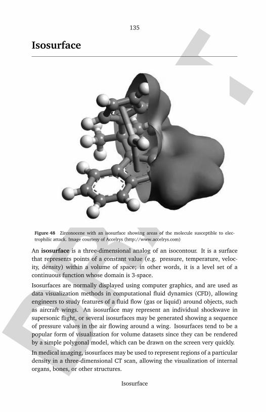
DRAF

T

135

Isosurface

Isosurface

Figure 48 Zirconocene with an isosurface showing areas of the molecule susceptible to elec-trophilic attack. Image courtesy of Accelrys (http://www.accelrys.com)

An isosurface is a three-dimensional analog of an isocontour. It is a surfacethat represents points of a constant value (e.g. pressure, temperature, veloc-ity, density) within a volume of space; in other words, it is a level set of acontinuous function whose domain is 3-space.

Isosurfaces are normally displayed using computer graphics, and are used asdata visualization methods in computational fluid dynamics (CFD), allowingengineers to study features of a fluid flow (gas or liquid) around objects, suchas aircraft wings. An isosurface may represent an individual shockwave insupersonic flight, or several isosurfaces may be generated showing a sequenceof pressure values in the air flowing around a wing. Isosurfaces tend to be apopular form of visualization for volume datasets since they can be renderedby a simple polygonal model, which can be drawn on the screen very quickly.

In medical imaging, isosurfaces may be used to represent regions of a particulardensity in a three-dimensional CT scan, allowing the visualization of internalorgans, bones, or other structures.

DRAF

T

136

Joint constraints

Numerous other disciplines that are interested in three-dimensional data of-ten use isosurfaces to obtain information about pharmacology, chemistry, geo-physics and meteorology.

A popular method of constructing an isosurface from a data volume is themarching cubes algorithm.

Source: http://en.wikipedia.org/wiki/Isosurface

Principal Authors: StoatBringer, The demiurge, Michael Hardy, RedWolf, Taw

Joint constraints

Joint constraints are rotational constraints on the joints of an artificial bonesystem. They are used in an inverse kinematics chain, for such things as 3Danimation or robotics. Joint constraints can be implemented in a number ofways, but the most common method is to limit rotation about the X, Y and Zaxis independently. An elbow, for instance, could be represented by limitingrotation on Y and Z axis to 0 degress of freedom, and constraining the X-axisrotation to 130 degrees of freedom.

To simulate joint constrains more accurately, dot-products can be used with anindependent axis to repulse the child bones orientation from the unreachableaxis. Limiting the orientation of the child bone to a border of vectors tangentto the surface of the joint, repulsing the child bone away from the border, canalso be useful in the precise restriction of shoulder movement.

Source: http://en.wikipedia.org/wiki/Joint_constraints

Principal Authors: Rofthorax, Dreadlocke, Salmar, Ravedave, Banana04131

DRAF

T

137

Lambertian reflectance

Lambertian reflectance

If a surface exhibits Lambertian reflectance, light falling on it is scatteredsuch that the apparent brightness of the surface to an observer is the sameregardless of the observer’s angle of view. More technically, the surface lumi-nance is the same regardless of angle of view. For example, unfinished woodexhibits roughly Lambertian reflectance, but wood finished with a glossy coatof polyurethane does not (depending on the viewing angle, specular highlightsmay appear at different locations on the surface). Not all rough surfaces areperfect Lambertian reflectors, but this is often a good approximation when thecharacteristics of the surface are unknown.

In computer graphics, Lambertian reflection is often used as a model for diffusereflection, and is calculated by taking the dot product of the surface’s normal-ized normal vector N and a normalized vector L pointing from the surface tothe light source. This number is then multiplied by the color of the surface andthe intensity of the light hitting the surface:

ID = L · N ∗ C ∗ IL,

where ID is the intensity of the diffusely reflected light (surface brightness), Cis the color and IL is the intensity of the incoming light. Because

L · N = |N ||L| cosα,

where α is the angle between the direction of the two vectors, the intensitywill be the highest if the normal vector points in the same direction as the lightvector (cos (0) = 1, the surface will be perpendicular to the direction of thelight), and the lowest if the normal vector is perpendicular to the light vector(cos (π) = 0, the surface runs parallel with the direction of the light).

Lambertian reflection is typically accompanied by specular reflection, wherethe surface luminance is highest when the observer’s angle is the same as theangle of the light source. This is simulated in computer graphics with →Phongshading.

Spectralon is a material which is designed to exhibit almost perfect Lambertianreflectance.

DRAF

T

138

Lambert’s cosine law

See also

• →Lambert’s cosine law• Specular reflection• →Diffuse reflection

Source: http://en.wikipedia.org/wiki/Lambertian_reflectance

Principal Authors: Srleffler, KYN, Pedrose, PAR, Pflatau


Lambert’s cosine law says that the total radiant power observed from a "Lam-bertian" surface is directly proportional to the cosine of the angle θ betweenthe observer’s line of sight and the surface normal. The law is also known asthe cosine emission law or Lambert’s emission law. It is named after JohannHeinrich Lambert, from his Photometria, published in 1760.

An important consequence of Lambert’s cosine law is that when an area ele-ment on the surface is viewed from any angle, it has the same radiance. Thismeans, for example, that to the human eye it has the same apparent brightness(or luminance). It has the same radiance because although the emitted pow-er from an area element is reduced by the cosine of the emission angle, theobserved size (solid angle) of the area element is also reduced by that sameamount, so that while the area element appears smaller, its radiance is thesame. For example, in the visible spectrum, the Sun is almost a Lambertianradiator, and as a result the brightness of the Sun is almost the same every-where on an image of the solar disk. Also, a black body is a perfect Lambertianradiator.

Lambertian reflectorsWhen an area element is radiating as a result of being illuminated by an exter-nal source, the irradiance (energy or photons/time/area) landing on that areaelement will be proportional to the cosine of the angle between the illuminat-ing source and the normal. A Lambertian reflector will then reflect this lightaccording to the same cosine law as a Lambertian emitter. This means thatalthough the radiance of the surface depends on the angle from the normal tothe illuminating source, it will not depend on the angle from the normal to theobserver. For example, if the moon were a Lambertian reflector, one would ex-pect to see its reflected brightness appreciably diminish towards the terminator

DRAF

T

139


due to the increased angle at which sunlight hit the surface. The fact that itdoes not diminish illustrates that the moon is not a Lambertian reflector, and infact tends to reflect more light into the oblique angles than would a Lambertianreflector.

Details of equal brightness effect

Figure 57 Figure 1: Emission rate (photons/s) in a normal and off-normal direction. The num-ber of photons/sec directed into any wedge is proportional to the area of the wedge.

DRAF

T

140


Figure 58 Figure 2: Observed intensity (photons/(s·cm2·sr)) for a normal and off-normal ob-server; dA 0 is the area of the observing aperture and dΩ is the solid angle subtended by theaperture from the viewpoint of the emitting area element.

This situation for a Lambertian reflector is illustrated in Figures 1 and 2. Forconceptual clarity we will think in terms of photons rather than energy or lu-minous energy. The wedges in the circle each represent an equal angle dΩ andthe number of photons per second emitted into each wedge is proportional tothe area of the wedge.

It can be seen that the height of each wedge is the diameter of the circle timescos(θ). It can also be seen that the maximum rate of photon emission perunit solid angle is along the normal and diminishes to zero for θ = 90. Inmathematical terms, the radiance along the normal is I photons/(s·cm2·sr)and the number of photons per second emitted into the vertical wedge is I dΩdA. The number of photons per second emitted into the wedge at angle θ isI cos(θ) dΩ dA.

Figure 2 represents what an observer sees. The observer directly above thearea element will be seeing the scene through an aperture of area dA 0 and thearea element dA will subtend a (solid) angle of dΩ0. We can assume withoutloss of generality that the aperture happens to subtend solid angle dΩ when"viewed" from the emitting area element. This normal observer will then berecording I dΩ dA photons per second and so will be measuring a radiance of

I0 = I dΩ dAdΩ0 dA0

photons/(s·cm2·sr).

DRAF

T

141

Level of detail (programming)

The observer at angle θ to the normal will be seeing the scene through thesame aperture of area dA 0 and the area element dA will subtend a (solid)angle of dΩ0 cos(θ). This observer will be recording I cos(θ) dΩ dA photonsper second, and so will be measuring a radiance of

I0 = I cos(θ) dΩ dAdΩ0 cos(θ) dA0

= I dΩ dAdΩ0 dA0

photons/(s·cm2·sr),

which is the same as the normal observer.

Source: http://en.wikipedia.org/wiki/Lambert%27s_cosine_law

Principal Authors: PAR, Dbenbenn, Srleffler, Oleg Alexandrov, Michael Hardy


In computer programming and computer graphics, level of detail involves de-creasing the detail of a model or object as it moves away from the viewer.Level of detail is used in computer and video games because it increases theefficiency of rendering by decreasing the polygon count — a desirable effect.The reduced visual quality of the model or object is, ideally, unnoticed due tothe distance of the object. This, of course, depends on the individual system orgame.

Black & White was one of the first games to use level of detail effects in itsrendering. Each map consisted of a single, large island, sometimes populatedwith hundreds of villagers. As the player zoomed the camera out, progressivelylower-detailed models were substituted for the villagers, buildings, and eventhe island itself. While not perfect, the technique allowed for a huge island tohave detail in close-ups, but still be visible without slow-down when zoomedout. Messiah used a similar technique and was released before Black & White.150

Halo 2 used level of detail adjustments to allow for much greater detail incutscenes and maps, but at the cost of a "detail pop-in" effect when a level orscene was first loaded. Models would appear to have little or no detail at first,with more detail suddenly appearing over time as the more detailed modelsand textures loaded.

In order to make the detail decrease less obvious, fog is commonly used incomputer and video games to reduce the visibility of details on the object,

http://pc.ign.com/articles/123/123117p1.html150

DRAF

T

142


simulating the haze that falls over distant objects in reality. When the object isout of the range of visibility, it won’t be rendered anymore.

One of the most common methods used in automatic level of detail construc-tion is based on the edge collapse transformation of a 3D mesh. Each pair ofvertices in the 3D mesh are given a weighted error metric based on curvatureor other criteria. The pair with the least given error is then merged/collapsedinto one vertex. This is repeated until the desired triangle count is reached.

Other more advanced methods include the creation of lists containing precal-culated edge collapse and vertex split values. Such lists can then be used forrealtime calculation of level of detail objects. This method is often referred toas progressive meshes.

More advanced level of detail runtime systems use algorithms that are ableto merge several 3D objects and simplify the merged objects in order to en-hance reduction. Such algorithms are referred to as hierarchical level of detailalgorithms.

External links

• Level of Detail for 3D Graphics151, by D. Luebke et. al.; one of the mostcomplete books on level of detail for computer graphics

• Phd disertation on hierarchical levels of details (PDF)152

• Donya research153; research and development of level of detail softwarecompany

Source: http://en.wikipedia.org/wiki/Level_of_detail_%28programming%29

Principal Authors: ZS, Drat, Jtalledo, Deepomega, GreatWhiteNortherner

http://lodbook.com/151

http://www.cs.unc.edu/~geom/HLOD/Dissertation/Dissertation.pdf152

http://www.donya.se153

DRAF

T

143

Low poly

Low poly

→Low poly is a term used by videogame creators, players and journalists aliketo describe a three-dimensional computer generated character or object thatappears to be lacking in polygons.

In computer technology, polygons are what designers typically use to createany three-dimensional object that is output to the screen. The polygons areusually triangles. The more triangles that are used to create an object, themore detailed it will appear, but the more computing power it will take torender the object. Because of this, designers of videogames often have to becreative or cut corners with their polygon budget (the number of polygons thatcan be rendered per frame in a scene). This leads to objects that are oftendescribed as being low poly.

Objects that are said to be low poly often appear blocky (square heads) andlacking in detail (no individual fingers). Objects that are supposed to be circu-lar or spherical are most obviously low poly, as the number of triangles neededto make a circle is high relative to other shapes, due to the curved line that isa circle.

The low poly issue is mostly confined to videogames and other software thatthe user manipulates in real time, e.g. the parts of a game that are playable.Low poly and polygon budgets are not an issue in, for example, computer-generated imagery effects like Gollum from the Lord of the Rings films or theentirety of Pixar animated films because they are created on large networksof computers called render farms. Each frame takes about an hour to create,despite the enormous computer power involved. This is why FMV sequencesin videogames look so much better than the games themselves.

Low poly is a phrase which is used relative to the time it is released. As com-puting power inevitably increases, the number of polygons that can be usedincreases as well. For example, Super Mario 64 would be considered low polytoday, but was considered a stunning achievement when it was released in1996.

See also

• →Bump mapping• →Normal mapping• Sprites• Nurbs

DRAF

T

144

MegaTexture

Source: http://en.wikipedia.org/wiki/Low_poly

Principal Authors: RJHall, David Levy, Plasmatics, Praetor alpha, Josh Parris

MegaTexture

MegaTexture refers to a texture mapping technique used in Splash Damage’supcoming game, Enemy Territory: Quake Wars. It was developed by id Soft-ware technical director John Carmack. MegaTexture is a design to eliminaterepeating textures over an environment. The original version of the Doom 3engine was criticized over its perceived inability to handle landscapes and largeoutdoor areas. The MegaTexture technology addresses this issue by introduc-ing a means to create expansive outdoor scenes. By painting a single massivetexture (About 32000x32000 pixels, or 1 gigapixel) covering the entire poly-gon map and highly detailed terrain, the desired effects can be achieved. TheMegaTexture can also store physical information about the terrain such as theamount of traction in certain areas or indicate what sound effect should beplayed when walking over specific terrain types on the map. i.e. walking onrock will sound different from walking on grass. It is expected that this willresult in a considerably more detailed scene than the majority of existing tech-nologies, using tiled textures, allow.

It has been suggested that MegaTexture technique is a modification of ClipMapping.

See also

• →Texture mapping• id Software• Enemy Territory: Quake Wars• Doom 3

External links

• id Software154

• Splash Damage155

http://www.idsoftware.com154

http://www.splashdamage.com155

DRAF

T

145

Mesa 3D

• John Carmack on MegaTexture156

• Arnout van Meer on Quake Wars157

Source: http://en.wikipedia.org/wiki/MegaTexture

Principal Authors: Mojohompo, R. Koot, Skrapion, Vahid83, Amren

Mesa 3D

Mesa 3D is an open source graphics library, initially developed by Brian Paul inAugust 1993, that provides a generic →OpenGL implementation for renderingthree-dimensional graphics on multiple platforms. Though Mesa is not an offi-cially licensed OpenGL implementation, the structure, syntax and semantics ofthe API is that of OpenGL.

Advantages

• In its current form, Mesa 3D is available and can be compiled on virtuallyall modern platforms.

• Though not an official OpenGL implementation for licensing reasons, theMesa 3D authors have worked to keep the API in line with the most currentOpenGL standards and conformance tests, as set forth by the OpenGL ARB.

• Mesa 3D is distributed under the MIT License.

• Whilst Mesa 3D supports several hardware graphics accelerators, it may al-so be compiled as a software-only renderer. Since it is also Open Sourced,it is possible to use it to study the internal workings of an →OpenGL-compatible renderer.

• It is sometimes possible to find subtle bugs in OpenGL applications by link-ing against Mesa 3D and using a conventional debugger to track problemsinto the lower level library.

http://www.gamerwithin.com/?view=article&article=1319&cat=2156

http://www.beyond3d.com/interviews/etqw/157

DRAF

T

146

Metaballs

External links

• Mesa 3D Homepage158 - Information and documentation for the latest ver-sion of Mesa 3D.

Source: http://en.wikipedia.org/wiki/Mesa_3D

Principal Authors: Imroy, SteveBaker, Agentsoo, Caiyu, Aegis Maelstrom

Metaballs

Figure 59 Two metaballs

Metaballs, in computer graphics terms, are organic-looking n-dimensional ob-jects. The technique for rendering metaballs was invented by Jim Blinn in theearly 1980s.

http://www.mesa3d.org/158

DRAF

T

147

Metropolis light transport

Each metaball is defined as a function in n-dimensions (ie. for three dimen-sions, f(x, y, z); three-dimensional metaballs tend to be most common). Athresholding value is also chosen, to define a solid volume. Then,∑

n

i=0metaball i(x, y, z) ≤ threshold

represents whether the volume enclosed by the surface defined by n metaballsis filled at (x, y, z) or not.

A typical function chosen for metaballs is f(x, y, z) = 1/((x − x0)2 + (y −y0)2 + (z− z0)2), where (x0, y0, z0) is the center of the metaball. However, dueto the divide, it is computationally expensive. For this reason, approximatepolynomial functions are typically used (examples?).

There are a number of ways to render the metaballs to the screen. The twomost common are brute force raycasting and the marching cubes algorithm.

2D metaballs used to be a very common demo effect in the 1990s. The effectis also available as an XScreensaver module.

Further reading

• Blinn, James F. "A Generalization of Algebraic Surface Drawing." ACMTransactions on Graphics 1(3), July 1982, pp. 235–256.

Source: http://en.wikipedia.org/wiki/Metaballs

Principal Authors: Iron Wallaby, Viznut, T-tus, Kibibu, Felsir

Metropolis light transport

This SIGGRAPH 1997 paper by Eric Veach and Leonidas J. Guibas describesan application of a variant of the Monte Carlo method called the Metropolis-Hastings algorithm to the rendering equation for generating images from de-tailed physical descriptions of three dimensional scenes.

The procedure constructs paths from the eye to a light source using bi-directional path tracing, then constructs slight modifications to the path. Somecareful statistical calculation (the Metropolis algorithm) is used to computethe appropriate distribution of brightness over the image. This procedure hasthe advantage, relative to bidirectional path tracing, that once a path has beenfound from light to eye, the algorithm can then explore nearby paths; thus

DRAF

T

148

Micropolygon

difficult-to-find light paths can be explored more thoroughly with the samenumber of simulated photons.

In short, the algorithm generates a path and stores the paths ’nodes’ in a list. Itcan then modify the path by adding extra nodes and creating a new light path.While creating this new path, the algorithm decides how many new ’nodes’ toadd and whether or not these new nodes will actually create a new path.

External link

• Metropolis project at Stanford159

Source: http://en.wikipedia.org/wiki/Metropolis_light_transport

Principal Authors: Pfortuny, Loisel, Aarchiba, The Anome, Levork

Micropolygon

In →3D computer graphics, a micropolygon is a polygon that is at least assmall as the size of a pixel in the output image. The concept of micropoly-gons was developed to be used by the Reyes algorithm. At rendering time,the geometric primitive is tessellated into a rectangular grid of tiny four-sidedpolygons or micropolygons. A shader later assigns colors to the vertices ofthese faces. Commonly the size of these micropolygons is the same as the areaof a pixel. Using micropolygons allows the renderer to create a highly detailedimage.

Shaders that operate on micropolygons can process an entire grid at once inSIMD fashion. This often leads to faster shader execution, and allows shadersto compute spatial derivatives (e.g. for texture filtering) by comparing valuesat neighboring micropolygon vertices.

A renderer that uses micropolygons can support displacement mapping simplyby perturbing micropolygon vertices during shading.

Further reading

• Steve Upstill: The RenderMan Companion: A Programmer’s Guide to Real-istic Computer Graphics, Addison-Wesley, ISBN 0-201-50868-0

• Anthony A. Apodaca, Larry Gritz: Advanced RenderMan: Creating CGI forMotion Pictures, Morgan Kaufmann Publishers, ISBN 1-55860-618-1

http://graphics.stanford.edu/papers/metro/159

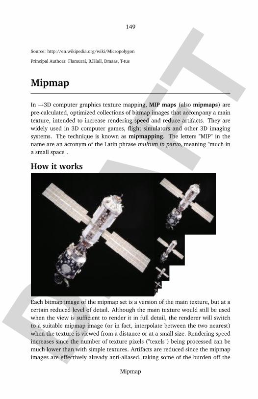
DRAF

T

149

Mipmap

Source: http://en.wikipedia.org/wiki/Micropolygon

Principal Authors: Flamurai, RJHall, Dmaas, T-tus

Mipmap

In →3D computer graphics texture mapping, MIP maps (also mipmaps) arepre-calculated, optimized collections of bitmap images that accompany a maintexture, intended to increase rendering speed and reduce artifacts. They arewidely used in 3D computer games, flight simulators and other 3D imagingsystems. The technique is known as mipmapping. The letters "MIP" in thename are an acronym of the Latin phrase multum in parvo, meaning "much ina small space".

How it works

Each bitmap image of the mipmap set is a version of the main texture, but at acertain reduced level of detail. Although the main texture would still be usedwhen the view is sufficient to render it in full detail, the renderer will switchto a suitable mipmap image (or in fact, interpolate between the two nearest)when the texture is viewed from a distance or at a small size. Rendering speedincreases since the number of texture pixels ("texels") being processed can bemuch lower than with simple textures. Artifacts are reduced since the mipmapimages are effectively already anti-aliased, taking some of the burden off the

DRAF

T

150

Mipmap

real-time renderer. Scaling down and up is made more efficient with mipmapsas well.

If the texture has a basic size of 256 by 256 pixels (textures are typically squareand must have side lengths equal to a power of 2), then the associated mipmapset may contain a series of 8 images, each one-fourth the size of the previousone: 128×128 pixels, 64×64, 32×32, 16×16, 8×8, 4×4, 2×2, 1×1 (a singlepixel). If, for example, a scene is rendering this texture in a space of 40×40pixels, then an interpolation of the 64×64 and the 32×32 mipmaps would beused. The simplest way to generate these textures is by successive averaging,however more sophisticated algorithms (perhaps based on signal processingand Fourier transforms) can also be used.

The increase in storage space required for all of these mipmaps is a third ofthe original texture, because the sum of the areas 1/4 + 1/16 + 1/256 + ...converges to 1/3. (This assumes compression is not being used.) This is amajor advantage to this selection of resolutions. However, in many instances,the filtering should not be uniform in each direction (it should be anisotropic,as opposed to isotropic), and a compromise resolution is used. If a higherresolution is used, the cache coherence goes down, and the aliasing is increasedin one direction, but the image tends to be clearer. If a lower resolution is used,the cache coherence is improved, but the image is overly blurry, to the pointwhere it becomes difficult to identify.

To help with this problem, nonuniform mipmaps (also known as rip-maps)are sometimes used. With a 16×16 base texture map, the rip-map resolutionswould be 16×8, 16×4, 16×2, 16×1, 8×16, 8×8, 8×4, 8×2, 8×1, 4×16, 4×8,4×4, 4×2, 4×1, 2×16, 2×8, 2×4, 2×2, 2×1, 1×16, 1×8, 1×4, 1×2 and 1×1.

The unfortunate problem with this approach is that rip-maps require four timesas much memory as the base texture map, and so rip-maps have been veryunpopular.

To reduce the memory requirement, and simultaneously give more resolutionsto work with, summed-area tables were conceived. Given a texture (tjk), wecan build a summed area table (sjk) as follows. The summed area table hasthe same number of entries as there are texels in the texture map. Then, define

smn :=∑

1≤j≤m, 1≤k≤n tjk

Then, the average of the texels in the rectangle (a1,b1] × (a2,b2] is given bysa2b2−sa1b2−sa2b1 +sa1b1

(a2−a1)(b2−b1)

DRAF

T

151

Morph target animation

However, this approach tends to exhibit poor cache behavior. Also, a summedarea table needs to have wider types to store the partial sums sjk than theword size used to store tjk. For these reasons, there isn’t any hardware thatimplements summed-area tables today.

A compromise has been reached today, called anisotropic mip-mapping. In thecase where an anisotropic filter is needed, a higher resolution mipmap is used,and several texels are averaged in one direction to get more filtering in thatdirection. This has a somewhat detrimental effect on the cache, but greatlyimproves image quality.

OriginMipmapping was invented by Lance Williams in 1983 and is described in hispaper Pyramidal parametrics. From the abstract: "This paper advances a ’pyra-midal parametric’ prefiltering and sampling geometry which minimizes aliasingeffects and assures continuity within and between target images." The "pyra-mid" can be imagined as the set of mipmaps stacked on top of each other.

See also

• Anti-aliasing

Source: http://en.wikipedia.org/wiki/Mipmap

Principal Authors: MIT Trekkie, RJHall, Spoon!, Mat-C, Tarquin, Grendelkhan

Morph target animation

Morph target animation (or per-vertex animation) is a method of 3D com-puter animation that is sometimes used in alternative to skeletal animation.Morph target animation is stored as a series of vertex positions. In eachkeyframe of the animation, the vertices are moved to a different position.

Depending on the renderer, the vertices will move along paths to fill in theblank time between the keyframes or the renderer will simply switch betweenthe different positions, creating a somewhat jerky look. The former is usedmore commonly.

There are advantages to using morph target animation over skeletal animation.The artist has more control over the movements because he or she can definethe individual positions of the vertices within a keyframe, rather than being

DRAF

T

152

Motion capture

constrained by skeletons. This can be useful for animation cloth, skin, andfacial expressions because it can be difficult to conform those things to thebones that are required for skeletal animation.

However, there are also disadvantages. Vertex animation is usually a lot moretime-consuming than skeletal animation because every vertex position wouldhave to be calculated. (3D models in modern computer and video games of-ten contain something to the order of 4,000-9,000 vertices.) Also, in methodsof rendering where vertices move from position to position during in-betweenframes, a distortion is created that doesn’t happen when using skeletal anima-tion. This is described by critics of the technique as looking "shaky." Howerver,there are some who like this slightly distorted look.

Not all morph target animation has to be done by actually editting vertex po-sitions. It is also possible to take vertex positions found in skeletal animationand then use those rendered as morph target animation.

Sometimes, animation done in one 3D application suite will need to be takeninto another for rendering. To avoid issues in export, animation will often beconverted from whatever format it was in to morph target animation. This issometimes necessary because things such as bones and special effects are notprogrammed using consistent systems among different 3D application suties.

See also

• Skeletal animation• Computer and video games• →3D computer graphics

Source: http://en.wikipedia.org/wiki/Morph_target_animation

Motion capture

Motion capture, or mocap, is a technique of digitally recording movementsfor entertainment, sports and medical applications.

It started as an analysis tool in biomechanics research, but has grown increas-ingly important as a source of motion data for computer animation as well aseducation, training and sports and recently for both cinema and video games.A performer wears a set of one type of marker at each joint: acoustic, inertial,LED, magnetic or reflective markers, or combinations, to identify the motion

DRAF

T

153

Motion capture

Figure 60 A dancer wearing a suit used in an optical motion capture system

of the joints of the body. Sensors track the position or angles of the mark-ers, optimally at least two times the rate of the desired motion. The motioncapture computer program records the positions, angles, velocities, accelera-tions and impulses, providing an accurate digital representation of the motion.This can reduce the costs of animation, which otherwise requires the animatorto draw each frame, or with more sophisticated software, key frames whichare interpolated by the software. Motion capture saves time and creates morenatural movements than manual animation, but is limited to motions that areanatomically possible. Some applications might require additional impossiblemovements like animated super hero martial arts.

Optical systems triangulate the 3D position of a marker with a number of cam-eras with high precision (sub-millimeter resolution or better). These systemsproduce data with 3 degrees of freedom for each marker, and rotational infor-mation must be inferred from the relative orientation of three or more markers;for instance shoulder, elbow and wrist markers providing the angle of the el-bow. A related technique match moving can derive 3D camera movement froma single 2D image sequence without the use of photogrammetry, but is oftenambiguous below centimeter resolution, due to the inability to distinguish pose

DRAF

T

154

Motion capture

and scale characteristics from a single vantage point. One might extrapolatethat future technology might include full-frame imaging from many cameraangles to record the exact position of every part of the actor’s body, clothing,and hair for the entire duration of the session, resulting in a higher resolutionof detail than is possible today. A newer technique discussed below uses higherresolution linear detectors to derive the one dimensional positions, requiringmore sensors and more computations, but providing higher resolutions (submillimeter down to 10 micrometres time averaged) and speeds than possibleusing area arrays 160 161 162.

Passive optical systems use reflective markers and triangulate each markerfrom its relative location on a 2D map with multiple cameras calibrated toprovide overlapping projections combined to calculate 3D positions. Data canbe cleaned up with the aid of kinematic constraints and predictive gap fillingalgorithms. Passive systems typically use sensors such as Micron’s 163 where thesensor captures an image of the scene, reduces it to bright spots and finds thecentroid. These 1.3 megapixel sensors can run at frame rates up to 60,000,000pixels per second divided by the resolution, so at 1.3 megapixels they can op-erate at 500 frames per second. The 4 megapixel sensor costs about $1,000and can run at 640,000,000 pixels per second divided by the applied resolu-tion. By decreasing the resolution down to 640 x 480, they can run at 2,000frames per second, but then trade off spatial resolution for temporal resolution.At full resolution they run about 166 frames per second, with about 200 LEDstrobes syncronized to the CMOS sensor. The ease of combining a hundreddollars worth of LEDs to a $1,000 sensor has made these system very popu-lar. Professional vendors have sophisticated software to reduce problems frommarker swapping since all markers appear identical. These systems are popularfor entertainment, biomechanics, engineering, and virtual reality applications;tracking a large number of markers and expanding the capture area with theaddition of more cameras. Unlike active marker systems and magnetic systems,passive systems do not require the user to wear wires or electronic equipment.Passive markers are usually spheres or hemispheres made of plastic or foam25 to 3mm in diameter with special retroreflective tape. This type of systemis the dominate favorite among entertainment and biomechanics groups cur-rently due to its ability to capture large numbers of markers at frame rates ashigh as 2000fps and high 3D accuracy. Active marker system run into a disad-vantage when marker counts climb as they perform "frame slicing", providing

http://www.ndigital.com160

http://www.phasespace.com/161

http://www.vicon.com/162

http://www.micron.com/products/imaging/products/MT9M413.html163

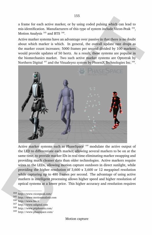
DRAF

T

155

Motion capture

a frame for each active marker, or by using coded pulsing which can lead tomis-identification. Manufacturers of this type of system include Vicon-Peak 164,Motion Analysis 165 and BTS 166.

Active marker systems have an advantage over passive in that there is no doubtabout which marker is which. In general, the overall update rate drops asthe marker count increases; 5000 frames per second divided by 100 markerswould provide updates of 50 hertz. As a result, these systems are popular inthe biomechanics market. Two such active marker systems are Optotrak byNorthern Digital 167 and the Visualeyez system by PhoeniX Technologies Inc.168.

Active marker systems such as PhaseSpace 169 modulate the active output ofthe LED to differentiate each marker, allowing several markers to be on at thesame time, to provide marker IDs in real time eliminating marker swapping andproviding much cleaner data than older technologies. Active markers requirewires to the LEDs, allowing motion capture outdoors in direct sunlight, whileproviding the higher resolution of 3,600 x 3,600 or 12 megapixel resolutionwhile capturing up to 480 frames per second. The advantage of using activemarkers is intelligent processing allows higher speed and higher resolution ofoptical systems at a lower price. This higher accuracy and resolution requires

http://www.viconpeak.com/164

http://www.motionanalysis.com165

http://www.bts.it166

http://www.ndigital.com167

http://www.ptiphoenix.com/168

http://www.phasespace.com/169

DRAF

T

156

Motion capture

more processing than older passive technologies, but the additional processingis done at the camera to improve resolution via a subpixel or centroid process-ing, providing both high resolution and high speed. By using newer processingand technology, these motion capture systems are about 1/3 the cost of oldersystems.

Magnetic systems, calculate position and orientation by the relative magneticflux of three orthogonal coils on both the transmitter and each receiver. The rel-ative intensity of the voltage or current of the three coils allows these systemsto calculate both range and orientation by meticulously mapping the trackingvolume. Since the sensor output is 6DOF, useful results can be obtained withtwo-thirds the number of markers required in optical systems; one on upperarm and one on lower arm for elbow position and angle. The markers are notoccluded by nonmetallic objects but are susceptible to magnetic and electricalinterference from metal objects in the environment, like rebar (steel reinforc-ing bars in concrete) or wiring, which affect the magnetic field, and electricalsources such as monitors, lights, cables and computers. The sensor responseis nonlinear, epecially toward edges of the capture area. The wiring from thesensors tends to preclude extreme performance movements. The capture vol-umes for magnetic systems are dramatically smaller than they are for opticalsystems. With the magnetic systems, there is a distinction between "AC" and"DC" systems: one uses square pulses, the other uses sine wave pulses. Twomagnetic systems are Ascension technology170 and Polhemus171.

A motion capture session records only the movements of the actor, not his vi-sual appearance. These movements are recorded as animation data which aremapped to a 3D model (human, giant robot, etc.) created by a computer artist,to move the model the same way. This is comparable to the older technique ofrotoscope where the visual appearance of the motion of an actor was filmed,then the film used as a guide for the frame by frame motion of a hand-drawnanimated character.

Inertial systems use devices such as accelerometers or gyroscopes to measurepositions and angles. They are often used in conjunction with other systemsto provide updates and global reference, since they only measure relativechanges, not absolute position.

RF (radio frequency) positioning systems are becoming more viable as higherfrequency RF devices allow greater precision than older RF technologies. Thespeed of light is 30 centimeters per nanosecond (billionth of a second), so a10 gigahertz (billion cycles per second) RF signal enables an accuracy of about

http://www.ascension-tech.com/170

http://www.polhemus.com/171

DRAF

T

157

Motion capture

3 centimeters. By measuring amplitude to a quarter wavelength, it is possibleto improve the resolution down to about 8 mm. To achieve the resolutionof optical systems, frequencies of 50 gigahertz or higher are needed, whichare almost as line of sight and as easy to block as optical systems. Multipathand reradiation of the signal are likely to cause additional problems, but thesetechnologies will be ideal for tracking larger volumes with reasonable accuracy,since the required resolution at 100 meter distances isn’t likely to be as high.

Mechanical motion capture systems directly track body joint angles and are of-ten referred to as exo-skeleton motion capture systems, due to the way the sen-sors are attached to the body. A performer attaches the skeletal-like structureto their body and as they move so do the articulated mechanical parts, mea-suring the performer’s relative motion. Mechanical motion capture systems arereal-time, relatively low-cost, free-of-occlusion, and wireless (untethered) sys-tems that have unlimited capture volume. Typically, they are rigid structuresof jointed, straight metal or plastic rods linked together with potentiometersthat articulate at the joints of the body. However, a newer and more flexibletake on exo-skeleton motion capture systems is the ShapeWrap II 172 system byMeasurand Inc.173ShapeWrap II offers a mocap system based on ShapeTapes 174

that flex. By conforming to limbs instead of following rigid paths, ShapeWrapII moves with the body to capture fine details of shape on a wide variety ofbody types.

http://www.measurand.com/products/ShapeWrap.html172

http://www.measurand.com/173

http://www.measurand.com/products/ShapeTape.html174

DRAF

T

158

Motion capture

The procedureIn the motion capture session, the movements of one or more actors are sam-pled many times per second. High resolution optical motion capture systemscan be used to sample body, facial and finger movement at the same time

If desired, a camera can pan, tilt, or dolly around the stage while the actor isperforming and the motion capture system can capture the camera and propsas well. This allows the computer generated characters, images and sets, tohave the same perspective as the video images from the camera. A computerprocesses the data and displays the movements of the actor, as inferred fromthe 3D position of each marker.

After processing, the software exports animation data, which computer anima-tors can associate with a 3D model and then manipulate using normal comput-er animation software such as Maya or 3D Studio Max. If the actor’s perfor-mance was good and the software processing was accurate, this manipulationis limited to placing the actor in the scene that the animator has created andcontrolling the 3D model’s interaction with objects.

AdvantagesMocap offers several advantages over traditional computer animation of a 3Dmodel:

• Mocap can take far fewer man-hours of work to animate a character. Oneactor working for a day (and then technical staff working for many daysafterwards to clean up the mocap data) can create a great deal of animationthat would have taken months for traditional animators.

• Mocap can capture secondary animation that traditional animators mightnot have had the skill, vision, or time to create. For example, a slight move-ment of the hip by the actor might cause his head to twist slightly. Thisnuance might be understood by a traditional animator but be too time con-suming and difficult to accurately represent, but it is captured accuratelyby mocap, which is why mocap animation often seems shockingly realisticcompared with hand animated models. Incidentally, one of the hallmarksof rotoscope in traditional animation is just such secondary "business."

• Mocap can accurately capture difficult-to-model physical movement. Forexample, if the mocap actor does a backflip while holding nunchaku by thechain, both sticks of the nunchucks will be captured by the cameras movingin a realistic fashion. A traditional animator might not be able to physicallysimulate the movement of the sticks adequately due to other motions by theactor. Secondary motion such as the ripple of a body as an actor is punched

DRAF

T

159

Motion capture

or is punching requires both higher speed and higher resolution as well asmore markers.

DisadvantagesOn the negative side, mocap data requires special programs and time to manip-ulate once captured and processed, and if the data is wrong, it is often easierto throw it away and reshoot the scene rather than trying to manipulate thedata. Many systems allow real time viewing of the data to decide if the takeneeds to be redone.

Another important point is that while it is common and comparatively easyto mocap a human actor in order to animate a biped model, applying motioncapture to animals like horses can be difficult.

Motion capture equipment costs tens of thousands of dollars for the digitalvideo cameras, lights, software, and staff to run a mocap studio, and this tech-nology investment can become obsolete every few years as better software andtechniques are invented. Some large movie studios and video game publishershave established their own dedicated mocap studios, but most mocap work iscontracted to individual companies that specialize in mocap.

ApplicationsVideo games use motion capture for football, baseball and basketball playersor the combat moves of a martial artist.

Movies use motion capture for CG effects, in some cases replacing tradition-al cell animation, and for completely computer-generated creatures, such asGollum, Jar-Jar Binks, and King Kong, in live-action movies.

Virtual Reality and Augmented Reality require real time input of the user’s po-sition and interaction with their environment, requiring more precision andspeed than older motion capture systems could provide. Noise and errorsfrom low resolution or low speed systems, and overly smoothed and filtereddata with long latency contribute to "simulator sickness" where the lag andmismatch between visual and vistibular cues and computer generated imagescaused nasea and discomfort.

High speed - high resolution active marker systems can provide smooth data atlow latency, allowing real time visualization in virtual and augmented realitysystems. The remaining challenge that is almost possible with powerful graphiccards is mapping the images correctly to the real perspectives to prevent imagemismatch.

Motion capture technology is frequently used in digital puppetry systems to aidin the performance of computer generated characters in real-time.

DRAF

T

160

Motion capture

Related techniquesFacial motion capture is utilized to record the complex movements in a humanface, especially while speaking with emotion. This is generally performed withan optical setup using multiple cameras arranged in a hemisphere at closerange, with small markers glued or taped to the actor’s face.

Performance capture is a further development of these techniques, where bothbody motions and facial movements are recorded. This technique was used inmaking of The Polar Express, where all actors were animated this way.

An alternative approach was developed by a Russian compa-ny VirtuSphere175, where the actor is given an unlimited walk-ing area through the use of a rotating sphere, similar to a

, which con-tains internal sensors recording the angular movements, removing the needfor external cameras and other equipment. Even though this technology couldpotentially lead to much lower costs for mocap, the basic sphere is only capa-ble of recording a single continuous direction. Additional sensors worn on theperson would be needed to record anything more.

http://www.virtusphere.net/175

DRAF

T

161

Motion capture

See also

• Animation• Rotoscope• Match moving, also known as "motion tracking"

External links

• Perspective Studios176- Motion Capture Studio located in New York.• LUKOtronic177 - Portable optical motion capture systems.• Motion Analysis178 - Maker of optical motion capture systems.• Vicon Peak179 - Maker of optical motion capture systems.• Audiomotion Studios180 - Award Winning Motion Capture Service Provider

Based in the UK.• VirtualCinematography.org181 - several papers on Universal Capture use in

Matrix films• Motion Reality Inc.182 - A company specializing in motion capture systems

and applications• Measurand Inc.183 - A company specializing in motion capture systems and

applications• Motion Reality Golf184 - A golf training application using motion capture

technology• Optical Motion Capture185 - Active Marker LED based real time motion

tracking hardware and software for VR, AR, Telerobotics, medical and en-tertainment applications.

• Giant Studios Inc.186 - A company specializing in motion capture systemsand software (Polar Express, Chronicles of Narnia)

• motionVR Corporation187 - A company that produces software for creatingsemi-3D models of real life locations.

http://www.perspectivestudios.com/176

http://www.LUKOtronic.com/177

http://www.motionanalysis.com/178

http://www.vicon.com/179

http://www.audiomotion.com/180

http://www.virtualcinematography.org/181

http://www.motionrealityinc.com/182


http://www.motionrealitygolf.com/184

http://www.PhaseSpace.com/185

http://www.giantstudios.com/186

http://www.motionVR.com187

DRAF

T

162

Motion capture

• VirtuSphere Inc.188 - A company designed an alternative way of motion cap-ture.

• Mocap.ca189 - Motion Capture resources and services including software andmotion capture data.

• House of Moves190 - Motion Capture Facility based in Los Angeles

Motion capture hardware

• LUKOtronic - Motion Capture Systems191 - Commercially available motioncapture systems and tools

• The ShapeWrap II & ShapeHand Motion Capture Systems192 - Commerciallyavailable motion capture systems and tools

• PhaseSpace Optical Motion Capture193 - Active Marker LED based real timemotion tracking hardware and software for VR, AR, Telerobotics, medicaland entertainment applications.

• PhoeniX Technologies Inc. - Real-time Motion Capture194 - Features the Vi-sualeyez real-time, active-optical motion capture system. Hardware andsoftware for diverse applications: biomechanics research, virtual environ-mnents, animation, game development, tele-robotics, and more.

Source: http://en.wikipedia.org/wiki/Motion_capture

Principal Authors: Tmcsheery, Myf, Tempshill, Plowboylifestyle, Paranoid, Lindosland, RobertM52,

Sergeyy, Michael Snow

http://www.virtusphere.net/188

http://www.mocap.ca/189

http://www.moves.com/190

http://www.LUKOtronic.com/191


http://www.PhaseSpace.com/193

http://www.ptiphoenix.com/194

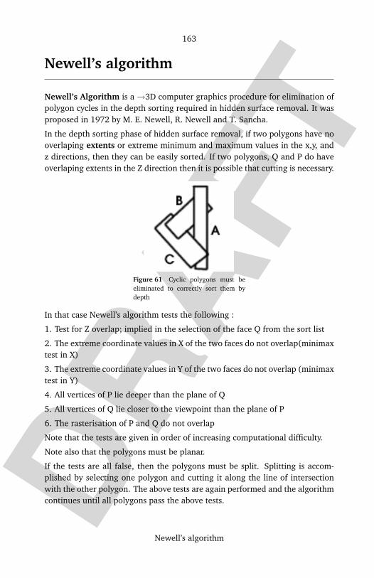
DRAF

T

163

Newell’s algorithm

Newell’s algorithm

Newell’s Algorithm is a →3D computer graphics procedure for elimination ofpolygon cycles in the depth sorting required in hidden surface removal. It wasproposed in 1972 by M. E. Newell, R. Newell and T. Sancha.

In the depth sorting phase of hidden surface removal, if two polygons have nooverlaping extents or extreme minimum and maximum values in the x,y, andz directions, then they can be easily sorted. If two polygons, Q and P do haveoverlaping extents in the Z direction then it is possible that cutting is necessary.

Figure 61 Cyclic polygons must beeliminated to correctly sort them bydepth

In that case Newell’s algorithm tests the following :

1. Test for Z overlap; implied in the selection of the face Q from the sort list

2. The extreme coordinate values in X of the two faces do not overlap(minimaxtest in X)

3. The extreme coordinate values in Y of the two faces do not overlap (minimaxtest in Y)

4. All vertices of P lie deeper than the plane of Q

5. All vertices of Q lie closer to the viewpoint than the plane of P

6. The rasterisation of P and Q do not overlap

Note that the tests are given in order of increasing computational difficulty.

Note also that the polygons must be planar.

If the tests are all false, then the polygons must be split. Splitting is accom-plished by selecting one polygon and cutting it along the line of intersectionwith the other polygon. The above tests are again performed and the algorithmcontinues until all polygons pass the above tests.

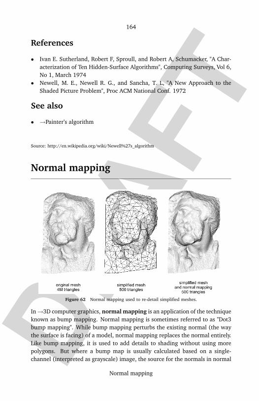
DRAF

T

164

Normal mapping

References

• Ivan E. Sutherland, Robert F, Sproull, and Robert A, Schumacker, "A Char-acterization of Ten Hidden-Surface Algorithms", Computing Surveys, Vol 6,No 1, March 1974

• Newell, M. E., Newell R. G., and Sancha, T. L, "A New Approach to theShaded Picture Problem", Proc ACM National Conf. 1972

See also

• →Painter’s algorithm

Source: http://en.wikipedia.org/wiki/Newell%27s_algorithm

Normal mapping

Figure 62 Normal mapping used to re-detail simplified meshes.

In→3D computer graphics, normal mapping is an application of the techniqueknown as bump mapping. Normal mapping is sometimes referred to as "Dot3bump mapping". While bump mapping perturbs the existing normal (the waythe surface is facing) of a model, normal mapping replaces the normal entirely.Like bump mapping, it is used to add details to shading without using morepolygons. But where a bump map is usually calculated based on a single-channel (interpreted as grayscale) image, the source for the normals in normal

DRAF

T

165

Normal mapping

mapping is usually a multichannel image (that is, channels for "red", "green"and "blue" as opposed to just a single color) derived from a set of more detailedversions of the objects.

Normal mapping is usually found in two varieties: object-space and tangent-space normal mapping. They differ in coordinate systems in which the normalsare measured and stored.

One of the most interesting uses of this technique is to greatly enhance theappearance of a low poly model exploiting a normal map coming from a highresolution model. While this idea of taking geometric details from a high res-olution model had been introduced in "Fitting Smooth Surfaces to Dense Poly-gon Meshes" by Krishnamurthy and Levoy, Proc. SIGGRAPH 1996, where thisapproach was used for creating displacement maps over nurbs, its applicationto more common triangle meshes came later. In 1998 two papers were pre-sented with the idea of transferring details as normal maps from high to lowpoly meshes: "Appearance Preserving Simplification", by Cohen et al. SIG-GRAPH 1998, and "A general method for recovering attribute values on sim-plified meshes" by Cignoni et al. IEEE Visualization ’98. The former presenteda particular constrained simplification algorithm that during the simplificationprocess tracks how the lost details should be mapped over the simplified mesh.The latter presented a simpler approach that decouples the high and low polyg-onal mesh and allows the recreation of the lost details in a way that is not de-pendent on how the low model was created. This latter approach (with someminor variations) is still the one used by most of the currently available tools.

How it worksTo calculate the lambertian (diffuse) lighting of a surface, the unit vector fromthe shading point to the light source is dotted with the unit vector normal tothat surface, and the result is the intensity of the light on that surface. Manyother lighting models also involve some sort of dot product with the normalvector. Imagine a polygonal model of a sphere - you can only approximate theshape of the surface. By using an RGB bitmap textured across the model, moredetailed normal vector information can be encoded. Each color channel in thebitmap (red, green and blue) corresponds to a spatial dimension (X, Y andZ). These spatial dimensions are relative to a constant coordinate system forobject-space normal maps, or to a smoothly varying coordinate system (basedon the derivatives of position with respect to texture coordinates) in the caseof tangent-space normal maps. This adds much more detail to the surface of amodel, especially in conjunction with advanced lighting techniques.

DRAF

T

166

Normal mapping

Normal mapping in computer entertainmentInteractive normal map rendering was originally only possible on PixelFlow, aparallel graphics machine built at the University of North Carolina at ChapelHill. It was later possible to perform normal mapping on high-end SGI worksta-tions using multi-pass rendering and frame buffer operations or on low end PChardware with some tricks using paletted textures. However, with the increas-ing processing power and sophistication of home PCs and gaming consoles,normal mapping has spread to the public consciousness through its use in sev-eral high-profile games, including: Far Cry (Crytek), Deus Ex: Invisible War(Eidos Interactive), Thief: Deadly Shadows (Eidos Interactive), The Chroniclesof Riddick: Escape from Butcher Bay (Vivendi Universal), Halo 2 (Microsoft),and Doom 3 (id Software), Half-Life 2 (Valve Software), Call of Duty 2 (Activi-sion), and Tom Clancy’s Splinter Cell: Chaos Theory (Ubisoft). It is also usedextensively in the upcoming third version of the Unreal engine (Epic Games).Normal mapping’s increasing popularity amongst video-game designers is dueto its combination of excellent graphical quality and decreased processing re-quirements versus other methods of producing similar effects. This decreasedprocessing requirement translates into better performance and is made possi-ble by distance-indexed detail scaling, a technique which decreases the detailof the normal map of a given texture (cf. mipmapping). Basically, this meansthat more distant surfaces require less complex lighting simulation. This inturn cuts the processing burden, while maintaining virtually the same level ofdetail as close-up textures.

Currently, normal mapping has been utilized successfully and extensively onboth the PC and gaming consoles. Initially, Microsoft’s Xbox was the onlyhome game console to fully support this effect, whereas other consoles usea software-only implementation as they don’t support it directly on hardware.Next generation consoles such as the Xbox360 rely heavily on normal mapping,and even use parallax mapping.

See also

• →Bump mapping• →Parallax mapping• →Displacement mapping• Linear algebra

DRAF

T

167

Normal mapping

External links

• GIMP normalmap plugin195

• Photoshop normalmap plugin196

• normal mapping tutorials197, Ben Cloward• Free xNormal normal mapper tool198, Santiago Orgaz• Maya normal mapping plugin199, Olivier Renouard• Normal Mapping with paletted textures200 using old OpenGL extensions.• Normal Mapping without hardware assistance201, Lux aeterna luceat eis

Amiga demo from Ephidrena• ZMapper202, Pixologic

Bibliography

• Fitting Smooth Surfaces to Dense Polygon Meshes203, Krishnamurthy andLevoy, SIGGRAPH 1996

• (PDF) Appearance-Preserving Simplification204, Cohen et. al, SIGGRAPH1998

• (PDF) A general method for recovering attribute values on simplifedmeshes205, Cignoni et al, IEEE Visualization 1998

• (PDF) Realistic, Hardware-accelerated Shading and Lighting206, Heidrichand Seidel, SIGGRAPH 1999

Source: http://en.wikipedia.org/wiki/Normal_mapping

Principal Authors: Xmnemonic, Tommstein, AlistairMcMillan, CobbSalad, ALoopingIcon, Andrew

pmk

http://nifelheim.dyndns.org/%7ecocidius/normalmap/195

http://developer.nvidia.com/object/photoshop_dds_plugins.html196

http://www.monitorstudios.com/bcloward/tutorials_normal_maps1.html197

http://www.santyesprogramadorynografista.net/projects.aspx198

http://www.drone.org/tutorials/displacement_maps.html199

http://vcg.isti.cnr.it/activities/geometryegraphics/bumpmapping.html200

http://ada.untergrund.net/showdemo.php?demoid=534&pv=1#Comments201

http://206.145.80.239/zbc/showthread.php?t=031281202

http://www-graphics.stanford.edu/papers/surfacefitting/203

http://www.cs.unc.edu/~geom/APS/APS.pdf204

http://vcg.isti.cnr.it/publications/papers/rocchini.pdf205

http://www.cs.ubc.ca/~heidrich/Papers/Siggraph.99.pdf206

DRAF

T

168

OpenGL

OpenGL

Figure 63 OpenGL official logo

OpenGL (Open Graphics Library) is a standard specification defining a cross-language cross-platform API for writing applications that produce →3D com-puter graphics (and 2D computer graphics as well). The interface consists ofover 250 different function calls which can be used to draw complex three-dimensional scenes from simple primitives. OpenGL was developed by Sili-con Graphics and is popular in the video games industry where it competeswith →Direct3D on Microsoft Windows platforms (see Direct3D vs. OpenGL).OpenGL is widely used in CAD, virtual reality, scientific visualization, informa-tion visualization, flight simulation and video game development.

SpecificationAt its most basic level, OpenGL is a specification, meaning it is simply a docu-ment that describes a set of functions and the precise behaviours that they mustperform. From this specification, hardware vendors create implementations— libraries of functions created to match the functions stated in the OpenGLspecification, making use of hardware acceleration where possible. Hardwarevendors have to meet specific tests to be able to qualify their implementationas an OpenGL implementation.

Efficient vendor-supplied implementations of OpenGL (making use of graphicsacceleration hardware to a greater or lesser extent) exist for Mac OS, Windows,Linux, many Unix platforms and PlayStation 3. Various software implementa-tions exist, bringing OpenGL to a variety of platforms that do not have ven-dor support. Notably, the open source library Mesa is a fully software-based

DRAF

T

169

OpenGL

graphics API which is code-compatible with OpenGL. However to avoid licens-ing costs associated with formally calling itself an OpenGL implementation, itclaims merely to be a "very similar" API.

The OpenGL specification is currently overseen by the OpenGL ArchitectureReview Board (ARB), which was formed in 1992. The ARB consists of a setof companies with a vested interest in creating a consistent and widely avail-able API. Voting members of the ARB as of April 2006 include 3D hardwaremanufacturers SGI, 3Dlabs, ATI Technologies, NVIDIA and Intel, and computermanufacturers IBM, Apple Computer, Dell, and Sun Microsystems. Microsoft,one of the founding members, left in March 2003. Aside from these corpora-tions, each year many other companies are invited to be part of the OpenGLARB for one-year terms. With so many companies involved with such a diverseset of interests, OpenGL has become very much a general-purpose API with awide range of capabilities.

According to current plans, control of OpenGL will pass to the Khronos Groupby the end of 2006. This is being done in order to improve the marketingof OpenGL, and to remove barriers between the development of OpenGL and→OpenGL ES.

Kurt Akeley and Mark Segal authored the original OpenGL specification. ChrisFrazier edited version 1.1. Jon Leech edited versions 1.2 through the presentversion 2.0.

DesignOpenGL serves two main purposes:

• To hide the complexities of interfacing with different 3D accelerators, bypresenting the programmer with a single, uniform API.

• To hide the differing capabilities of hardware platforms, by requiring thatall implementations support the full OpenGL feature set (using softwareemulation if necessary).

OpenGL’s basic operation is to accept primitives such as points, lines and poly-gons, and convert them into pixels. This is done by a graphics pipeline knownas the OpenGL state machine207. Most OpenGL commands either issue prim-itives to the graphics pipeline, or configure how the pipeline processes theseprimitives. Prior to the introduction of OpenGL 2.0, each stage of the pipelineperformed a fixed function and was configurable only within tight limits but inOpenGL 2.0 several stages are fully programmable using →GLSL.

http://www.opengl.org/documentation/specs/version1.1/state.pdf207

DRAF

T

170

OpenGL

OpenGL is a low-level, procedural API, requiring the programmer to dictatethe exact steps required to render a scene. This contrasts with descriptive(aka scene graph or retained mode) APIs, where a programmer only needs todescribe a scene and can let the library manage the details of rendering it.OpenGL’s low-level design requires programmers to have a good knowledge ofthe graphics pipeline, but also gives a certain amount of freedom to implementnovel rendering algorithms.

OpenGL has historically been influential on the development of 3D accelera-tors, promoting a base level of functionality that is now common in consumer-level hardware:

• Rasterised points, lines and polygons as basic primitives• A transform and lighting pipeline• →Z-buffering• →Texture mapping• Alpha blending

Many modern 3D accelerators provide functionality far above this baseline, butthese new features are generally enhancements of this basic pipeline ratherthan radical reinventions of it.

ExampleWe first clear the color buffer, in order to start with a blank canvas:

glClear( GL COLOR BUFFER BIT );

We now set the modelview matrix, which controls the position of the camerarelative to the primitives we render. We move it backwards 3 units along the Zaxis, which leaves it pointing towards the origin:

glMatrixMode( GL MODELVIEW ); /* Subsequent matrix com-

mands will affect the modelview matrix */

glLoadIdentity(); /* Initialise the modelview

to identity */

glTranslatef( 0, 0, -3 ); /* Translate the modelview 3

units along the Z axis */

The projection matrix governs the perspective effect applied to primitives, andis controlled in a similar way to the modelview matrix:

DRAF

T

171

OpenGL

glMatrixMode( GL PROJECTION ); /* Subsequent matrix com-

mands will affect the projection matrix */

glLoadIdentity(); /* Initialise the projection

matrix to identity */

glFrustum( -1, 1, -1, 1, 1, 1000 ); /* Apply a perspective-

projection matrix */

Finally, we issue a polygon - a green square oriented in the XY plane:

glBegin( GL POLYGON ); /* Begin issuing a polygon

*/

glColor3f( 0, 1, 0 ); /* Set the current color to

green */

glVertex3f( -1, -1, 0 ); /* Issue a vertex */

glVertex3f( -1, 1, 0 ); /* Issue a vertex */

glVertex3f( 1, 1, 0 ); /* Issue a vertex */

glVertex3f( 1, -1, 0 ); /* Issue a vertex */

glEnd(); /* Finish issuing the poly-

gon */

DocumentationPart of the popularity of OpenGL is the excellence of its official documentation.

The OpenGL ARB released a series of manuals along with the specificationwhich have been updated to track changes in the API. These are almost univer-sally known by the colors of their covers:

• The Red Book - The OpenGL Programmer’s guide. ISBN 0321335732• : A readable tutorial and reference book - this is a ’must have’ book for

OpenGL programmers.• The Blue Book - The OpenGL Reference manual. ISBN 032117383X• : Essentially a hard-copy printout of the man pages for OpenGL.• : Includes a poster-sized fold-out diagram showing the structure of an ide-

alised OpenGL implementation.• The Green Book - Programming OpenGL for the X Window System. ISBN

0201483599• : A book about X11 interfacing and GLUT.• The Alpha Book (which actually has a white cover) - OpenGL Programming

for Windows 95 and Windows NT. ISBN 0201407094• : A book about interfacing OpenGL to Microsoft Windows.

Then, for OpenGL 2.0 and beyond:

DRAF

T

172

OpenGL

• The Orange Book - The OpenGL Shading Language. ISBN 0321334892• : A readable tutorial and reference book for GLSL.

ExtensionsThe OpenGL standard allows individual vendors to provide additional func-tionality through extensions as new technology is created. Extensions may in-troduce new functions and new constants, and may relax or remove restrictionson existing OpenGL functions. Each vendor has an alphabetic abbreviation thatis used in naming their new functions and constants. For example, NVIDIA’sabbreviation (NV) is used in defining their proprietary function glCombinerPa-rameterfvNV() and their constant GL_NORMAL_MAP_NV. It may happen thatmore than one vendor agrees to implement the same extended functionality.In that case, the abbreviation EXT is used. It may further happen that theArchitecture Review Board "blesses" the extension. It then becomes known asa standard extension, and the abbreviation ARB is used. The first ARB ex-tension was GL_ARB_multitexture, introduced in version 1.2.1. Following theofficial extension promotion path, multitexturing is no longer an optionally im-plemented ARB extension, but has been a part of the OpenGL core API sinceversion 1.3.

Before using an extension a program must first determine its availability, andthen obtain pointers to any new functions the extension defines. The mech-anism for doing this is platform-specific and libraries such as →GLEW and→GLEE exist to simplify the process.

Specifications for nearly all extensions can be found at the official extensionregistry 208.

Associated utility librariesSeveral libraries are built on top of or beside OpenGL to provide features notavailable in OpenGL itself. Libraries such as →GLU can always be found withOpenGL implementations, and others such as GLUT and SDL have grown overtime and provide rudimentary cross platform windowing and mouse function-ality and if unavailable can easily be downloaded and added to a developmentenvironment. Simple graphical user interface functionality can be found inlibraries like →GLUI or FLTK. Still others libraries like AUX are deprecated li-braries that have been superseded by functionality commonly available in morepopular libraries, but code still exists out there particularly in simple tutorials.Other libraries have been created to provide OpenGL application developersa simple means of managing OpenGL extensions and versioning, examples of

http://oss.sgi.com/projects/ogl-sample/registry/208

DRAF

T

173

OpenGL

these libraries include →GLEW "The OpenGL Extension Wrangler Library" and→GLEE "The OpenGL Easy Extension library".

In addition to the aforementioned simple libraries other higher level object ori-ented scene graph retained mode libraries exist such as →PLIB, OpenScene-Graph, and OpenGL Performer, these are available as cross platform OpenSource or proprietary programming interfaces written on top of OpenGL andsystems libraries to enable the creation of real-time visual simulation applica-tions.

→Mesa 3D (209) is an Open Sourced implementation of OpenGL. It supportspure software rendering as well as providing hardware acceleration for several3D graphics cards under Linux. As of February 2 2006 it implements the 1.5standard, and provides some of its own extensions for some platforms.

BindingsIn order to emphasize its multi-language and multi-platform characteristics,various bindings and ports have been developed for OpenGL in many lan-guages. Most notably, the Java 3D library can rely on OpenGL for its hardwareacceleration. Direct bindings are also available like the Lightweight Java GameLibrary210 which has a direct binding of OpenGL for Java and other game re-lated components. Very recently, Sun has released beta versions of the JOGLsystem, which provides direct bindings to C OpenGL commands, unlike Java3D which does not provide such low level support. The OpenGL official page 211

lists various bindings for Java, Fortran 90, Perl, Pike, Python, Ada, and VisualBasic. Bindings are also available for C++ and C#, see 212.

Higher level functionalityOpenGL was designed to be graphic output-only: it provides only renderingfunctions. The core API has no concept of windowing systems, audio, print-ing to the screen, keyboard/mouse or other input devices. While this seemsrestrictive at first, it allows the code that does the rendering to be completelyindependent of the operating system it is running on, allowing cross-platformdevelopment. However some integration with the native windowing systemis required to allow clean interaction with the host system. This is performedthrough the following add-on APIs:

http://www.mesa3d.org209

http://lwjgl.org/210

http://www.opengl.org/211

http://www.exocortex.org/3dengine/212

DRAF

T

174

OpenGL

• GLX - X11 (including network transparency)• WGL - Microsoft Windows

Additionally the GLUT and SDL libraries provide functionality for basic win-dowing using OpenGL, in a portable manner. Mac OS X has three APIs to getOpenGL support: AGL for Carbon, NSOpenGL for Cocoa and CGL for lower-level access.

HistoryToday the digital generation of animated scenes in three dimensions is a reg-ular fixture in everyday life. Scientists utilize computer graphics to analyzesimulations of every possibility. Engineers and architects design virtual modelsusing computer graphics. Movies employ computer graphics to create stunningspecial effects or entire animated films. And over the past few years, comput-er games have brought computer graphics technology to regular consumers,using graphics to bring their players into worlds that could never exist.

Bringing digital graphics technology to such widespread use was not withoutits challenges. Fifteen years ago, developing software that could function witha wide range of graphics hardware and all of their different interfaces wastime consuming. Each team of programmers developed interfaces separately,and there was consequently much duplicated code. This was hindering thegrowing industry of computer graphics.

Silicon Graphics Incorporated specializes in the creation of specialized graphicshardware and software. By the early 1990’s, SGI had become the world leaderin 3D graphics, and its programming API, IrisGL, had become a defacto indus-try standard, over-shadowing the open-standards-based PHIGS. There wereseveral reasons for the market superiority: SGI usually had the best and fastesthardware; the IrisGL programming interface (API) was elegant, easy-to-use,and, importantly, supported immediate-mode rendering. By contrast, PHIGSwas clunky, hard to use, and was several generations behind IrisGL in func-tion and capability, primarily due to the dysfunctional PHIGS standardizationprocess. None-the-less, competing vendors, including Sun, Hewlett-Packardand IBM were able to bring to market credible 3D hardware, supported byproprietary extensions to PHIGS. By the early 90’s, 3D graphics hardware tech-nology was fairly well understood by a large number of competitors and wasno longer a discriminating factor in computer systems purchases. Thus, ratherthan prolonging a contentious and dangerous fight between IrisGL and PHIGS,SGI sought to turn a defacto standard into a true open standard.

The IrisGL API itself wasn’t suitable for opening (although it had been previous-ly licensed to IBM and others), in part because it had accumulated cruft over

DRAF

T

175

OpenGL

the years. For example, it included a windowing, keyboard and mouse API,in part because it was developed before the X11 Window System versus Sun’sNeWS battle had resolved. Thus, the API to be opened needed to be cleanedup. In addition, IrisGL had a large software vendor (ISV) portfolio; the changeto the OpenGL API would keep ISV’s locked onto SGI (and IBM) hardwarefor a few years while market support for OpenGL matured. Meanwhile, SGIwould continue to try to maintain a vendor lock by pushing the higher-leveland proprietary Iris Inventor and Iris Performer programming API’s.

The result is known as OpenGL. OpenGL standardised access to hardware, andpushed the development responsibility of hardware interface programs, some-times called device drivers, to hardware manufacturers and delegated window-ing functions to the underlying operating system. With so many different kindsof graphic hardware, getting them all to speak the same language in this wayhad a remarkable impact by giving software developers a higher level platformfor 3D-software development.

In 1992, SGI led the creation of the OpenGL architectural review board(OpenGL ARB), the group of companies that would maintain and expand theOpenGL specification for years to come. OpenGL evolved from (and is verysimilar in style to) SGI’s earlier 3D interface, IrisGL. One of the restrictions ofIrisGL was that it only provided access to features supported by the underlyinghardware. If the graphics hardware did not support a feature, then the appli-cation could not use it. OpenGL overcame this problem by providing supportin software for features unsupported by hardware, allowing applications to useadvanced graphics on relatively low-powered systems.

In 1994 SGI played with the idea of releasing something called "→OpenGL++"which included elements such as a scene-graph API (presumably based aroundtheir Performer technology). The specification was circulated among a fewinterested parties - but never turned into a product.

When →Direct3D was released in 1995, Microsoft, SGI, and Hewlett-Packardinitiated the Fahrenheit project, which was a joint effort with the goal of unify-ing the OpenGL and Direct3D interfaces - and again, adding a scene-graph API.It initially showed some promise of bringing order to the world of interactive3D computer graphics APIs, but on account of financial constraints at SGI andgeneral lack of industry support it was abandoned. The engineers involved atSGI held a beach party in celebration - complete with bonfires on which theyburned piles of Fahrenheit documentation.

DRAF

T

176

OpenGL

OpenGL 2.0OpenGL 2.0 was conceived by 3Dlabs to address concerns that OpenGL wasstagnating and lacked a strong direction. 3Dlabs proposed a number of ma-jor additions to the standard, the most significant of which was →GLSL (theOpenGL Shading Language, also slang). This would enable the programmer toreplace the OpenGL fixed-function vertex and fragment pipelines with shaderswritten in a C-like language, massively expanding the range of graphical ef-fects possible. GLSL was notable for making relatively few concessions to thelimitations of the hardware then available; this harkened back to the earliertradition of OpenGL setting an ambitious, forward-looking target for 3D accel-erators rather than merely tracking the state of currently available hardware.The final OpenGL 2.0 specification 213 includes support for GLSL, but omitsmany of the other features originally proposed which were deferred to laterversions of OpenGL (although many are now available as extensions).

Sample renderings

See also

• →GLSL - OpenGL’s shading language• Cg - nVidia’s shading language that works with OpenGL• Java OpenGL - Java bindings for OpenGL• →OpenGL ES - OpenGL for embedded systems• OpenAL - The Open Audio Library - designed to work well with OpenGL.• OpenSL ES - Another audio library.• →Graphics pipeline

OpenGL support libraries

• GLUT - The OpenGL utility toolkit.• →GLU - Some additional functions for OpenGL programs.

Other graphics API’s

• →Mesa 3D - An OpenSourced implementation of OpenGL.• →Direct3D and →Comparison of Direct3D and OpenGL - A competitor to

OpenGL.

http://www.opengl.org/documentation/specs/version2.0/glspec20.pdf213

DRAF

T

177

OpenGL

• Light Weight Java Game Library• VirtualGL

Further reading

• Richard S. Wright Jr. and Benjamin Lipchak: OpenGL Superbible, ThirdEdition, Sams Publishing, 2005, ISBN 0-67232-601-9

• Astle, Dave and Hawkins, Kevin: Beginning OpenGL Game Programming,Course Technology PTR, ISBN 1-59200-369-9

• Fosner, Ron: OpenGL Programming for Windows 95 and Windows NT, Ad-dison Wesley, ISBN 0-20140-709-4

• Kilgard, Mark: OpenGL for the X Window System, Addison-Wesley, ISBN0-20148-359-9

• Lengyel, Eric: The OpenGL Extensions Guide, Charles River Media, ISBN1-58450-294-0

• OpenGL Architecture Review Board, et al: OpenGL Reference Manual: TheOfficial Reference Document to OpenGL, Version 1.4, Addison-Wesley, ISBN0-32117-383-X

• OpenGL Architecture Review Board, et al: OpenGL Programming Guide:The Official Guide to Learning OpenGL, Version 2, Fifth Edition, Addison-Wesley, ISBN 0-32133-573-2

• Rost, Randi J.: OpenGL Shading Language, Addison-Wesley, ISBN 0-32119-789-5

External links


• Official OpenGL wiki215

• SGI’s OpenGL website216

• Red Book217 - Online copy of an early edition of The OpenGL ProgrammingGuide.

• Blue Book218 - Online copy of an early edition of The OpenGL ReferenceManual.

• MSDN219 - Microsoft’s OpenGL reference

http://www.opengl.org/214

http://www.opengl.org/wiki215

http://www.sgi.com/products/software/opengl/216

http://www.opengl.org/documentation/red_book/217

http://www.opengl.org/documentation/blue_book/218

http://msdn.microsoft.com/library/default.asp?url=/library/en-us/opengl/apxb4_82lh.asp219

DRAF

T

178

OpenGL++

• OpenGL 2.0 specification220 (PDF)• OpenGL tutorials, software, etc221 at the Open Directory Project

Source: http://en.wikipedia.org/wiki/OpenGL

Principal Authors: SteveBaker, 0waldo, Klassobanieras, Haakon, Imroy, Robertbowerman, Stoat-

Bringer, BSTRhino, Fresheneesz, Flamurai

OpenGL++

OpenGL++ was intended to be a powerful layer above the →OpenGL 3Dgraphics system written in C++ that supported object-oriented data structures.The project started as the result of a partnership between SGI, IBM and Intel(and later Digital Equipment Corporation as well) to provide a higher levelAPI than the "bare metal" support of OpenGL. Work on OpenGL++ endedwhen SGI decided to partner with Microsoft instead, leading to the Fahrenheitproject, which also died.

DevelopmentOpenGL++ (OGL++) was intended to offer a selection of routines and stan-dardized data structures to dramatically simplify writing "real" programs usingOpenGL. Instead of the programmer having to keep track of the objects in the3D world and make sure they were culled properly, OpenGL++ would includeits own scene graph system and handle many of the basic manipulation dutiesfor the programmer. In addition, OGL++ included a system for modifying thescene graph on the fly, re-arranging it for added performance.

Much of OGL++ was a combination of ideas from earlier SGI projects in thesame vein, namely →Open Inventor which offered ease-of-use, and OpenGLPerformer which was written separately from Inventor to deliver a system thatoptimized scene graphs for increased performance and exploited scalable ar-chitectures. It was later intended that a new design could get the best of bothworlds while forming the underlying framework for several projects includingCAD, image processing, visual simulation, scientific visualization and user in-terfaces or 3D manipulators allowing them to interoperate, thereby offeringboth rapid development and high performance.

http://www.opengl.org/documentation/specs/version2.0/glspec20.pdf220

http://dmoz.org/Computers/Programming/Graphics/Libraries/OpenGL/221

DRAF

T

179

OpenGL++

SGI had already almost completed one effort to merge the functionality ofscene graphsCosmo 3D, Cosmo 3D was in fact the spinoff from an earlier col-laboration with Sun which was supposed to produce a scene graph for Java inconjunction with SGI’s new scene graph, Sun and SGI went their separate wayswith Java3D and Cosmo3D. When SGI announced the OGL++ effort, theyhalted development of Cosmo3D when it had just reached a beta release. Bythen a CAD/"Large Model Visualization" layer of functionality called OpenGLOptimizer had already been implemented on Cosmo3D and then released asa product. Other "front end" packages like, Cosmo Code, a VRML authoringtool, were produced by a different division and use of the Cosmo name wasmerely part of a broader marketing strategy, it ran on OpenGL. OGL++ wasintended to be a cleaned up and more flexible version of Cosmo3D, most of theCosmo3D team started work on OGL++ and a lot of the effort was aimed at aspecification and implementation that could deliver on the promise of a trulypowerful yet generic scene graph.

At the endIn the end, there is little to show for any of these efforts. Parnerships with SunMicrosystems, Intel and IBM and Microsoft all led to nothing as SGI jumpedfrom project to project. In retrospect, SGI reacted badly to a rapidly changingenvironment. An internal desire to create a new improved generic but exten-sible scene graph was constantly sidetracked by a belief that SGI couldn’t go italone. Partnerships were formed and later abandoned due to irreconcilable dif-ferences or simply as priorities and internal pressures shifted. OGL++ was themost nacent of these efforts and although it was the option that rapidly gainedthe strongest interest the power of the idea forced an unholy alliance betweenMicrosoft and SGI in the form of Fahrenheit, SGI joining because of its longheld belief that it couldn’t go it alone and Microsoft because it wanted to avertthe possibility of a truly open 3D scene graph. Ancillary issues like powerfulCAD APIs running on Cosmo3D complicated the picture. In the final analysisthe new unified scene graph concept was bounced from project to project, andeventually died in 2000 when Fahrenheit was killed.

Today, no such standardized scene graph exists, and SGI has all but exited theAPI world. SGI has released the earlier Open Inventor code into open source,but the source to OGL++ was never completed to any satisfactory degree.No specification exists and as with OpenGL the spec and idea behind such anopen platform would have been what lent it it’s lasting value, not a singleimplementation of a scene graph idea.

Source: http://en.wikipedia.org/wiki/OpenGL%2B%2B

DRAF

T

180

OpenGL ES

Principal Authors: Maury Markowitz, Tim Starling, Michael Hardy, Heron, Engwar, Zondor, Jwest-

brook, Nikola Smolenski

OpenGL ES

OpenGL ES (OpenGL for Embedded Systems) is a subset of the →OpenGL3D graphics API designed for embedded devices such as mobile phones, PDAs,and video game consoles. It is defined and promoted by the Khronos Group,graphics hardware and software industry consortium interested in open APIsfor graphics and multimedia.

In creating OpenGL ES 1.0 much functionality has been stripped from the orig-inal OpenGL API and a little bit added, two of the more significant differencesbetween OpenGL ES and OpenGL are the removal of the glBegin–glEnd callingsemantics for primitive rendering (in favor of vertex arrays) and the introduc-tion of fixed-point data types for vertex coordinates and attributes to bettersupport the computational abilities of embedded processors, which often lackan FPU. Many other areas of functionality have been removed in version 1.0 toproduce a lightweight interface: for example, quad and polygon primitive ren-dering, texgen, line and polygon stipple, polygon mode, antialiased polygonrendering (with alpha border fragments, not multisample), ARB_Image classpixel operation functionality, bitmaps, 3D texture, drawing to the frontbuffer,accumulation buffer, copy pixels, evaluators, selection, feedback, display lists,push and pop state attributes, two-sided lighting, and user defined clip planes.

Several versions of the OpenGL ES specification now exist. OpenGL ES 1.0is drawn up against the OpenGL 1.3 specification, OpenGL ES 1.1 is definedrelative to the OpenGL 1.5 specification and OpenGL ES 2.0 is defined rela-tive to the OpenGL 2.0 specification. Version 1.0 and 1.1 both have commonand common lite profiles, the difference being that the common lite profileonly supports fixed-point in lieu of floating point data type support, whereascommon supports both.

OpenGL ES 1.1 adds to the OpenGL ES 1.0 functionality by introducing ad-ditional features such as mandatory support for multitexture, better multitex-ture support (with combiners and dot product texture operations), automaticmipmap generation, vertex buffer objects, state queries, user clip planes, andgreater control over point rendering.

The common profile for OpenGL ES 2.0, publicly released in August 2005,completely eliminates all fixed-function API support in favor of an entirely pro-grammable model, so features like the specification of surface normals in the

DRAF

T

181

OpenGL ES

API for use in a lighting calculation are eliminated in favor of abstract variables,the use of which is defined in a shader written by the graphics programmer.

OpenGL ES also defines an additional safety-critical profile that is intended tobe testable and demonstrably robust subset for safety-critical embedded appli-cations such as glass cockpit avionics displays.

OpenGL ES has been chosen as the official graphics API used for PlayStation 3gaming platform development and as the official 3D graphics API in SymbianOS.

Further reading

• Astle, Dave and David Durnil: OpenGL ES Game Development, CourseTechnology PTR, ISBN 1-592-00370-2

External links


• Open Source Software Implementation of OpenGL ES 1.0223

• ALT Software’s Commercial Implementation of OpenGL ES224

• A Swedish wiki dedicated to OpenGL/OpenGL ES and the developmentround it.225

Source: http://en.wikipedia.org/wiki/OpenGL_ES

Principal Authors: Flamurai, Gaius Cornelius, Nova77, Cmdrjameson, Orderud

http://www.khronos.org/opengles/222

http://ogl-es.sourceforge.net/223

http://www.altsoftware.com/products/opengl/224

http://www.opengl.se225

DRAF

T

182

OpenGL Utility Toolkit

OpenGL Utility Toolkit

This article is about the OpenGL toolkit. GLUT can also stand for glucosetransporter.

The →OpenGL Utility Toolkit (GLUT) is a library of utilities for OpenGL pro-grams, which primarily perform system-level I/O with the host operating sys-tem. Functions performed include window definition, window control, andmonitoring of keyboard and mouse input. Routines for drawing a number ofgeometric primitives (both in solid and wireframe mode) are also provided,including cubes, spheres, and the →Utah teapot. GLUT even has some limitedsupport for creating pop-up windows.

GLUT was written by Mark J. Kilgard, author of OpenGL Programming for theX Window System and The CG Tutorial: The Definitive Guide to ProgrammableReal-Time Graphics while he was working for Silicon Graphics Inc.

The two aims of GLUT are to allow the creation of rather portable code betweenoperating systems (GLUT is cross-platform) and to make learning OpenGLeasier. Getting started with OpenGL programming while using GLUT oftentakes only a few lines of code and requires no knowledge of operating system–specific windowing APIs.

All GLUT functions start with the glut prefix (for example, glutPostRedisplayrerenders the current screen).

freeglut and its spin-off, OpenGLUT, are free software alternatives to GLUT.Freeglut attempts to be a fairly exact clone, OpenGLUT adds a number of newfeatures to the API. Both have the advantage of licensing that permits users tomodify and redistribute the library.

See also

• →GLU• →GLUI

External links

• GLUT documentation226

• OpenGLUT227

• FreeGLUT228

http://www.opengl.org/documentation/specs/glut/spec3/spec3.html226

http://openglut.sourceforge.net/227

DRAF

T

183

Open Inventor

Source: http://en.wikipedia.org/wiki/OpenGL_Utility_Toolkit

Principal Authors: SteveBaker, Orderud, Elie De Brauwer, MarSch, Bogdangiusca

Open Inventor

Open Inventor, originally IRIS Inventor, is a C++ object oriented “retainedmode” 3D graphics API designed by SGI to provide a higher layer of program-ming for →OpenGL. Its main goals are better programmer convenience andefficiency.

Early historyAround 1988–1989, Wei Yen asked Rikk Carey to lead the IRIS Inventor project.Their goal was to create a toolkit that made developing 3D graphics applica-tions easier to do. The strategy was based on the premise that people werenot developing enough 3D applications with OpenGL because it was too time-consuming to do so with the low-level interface provided by OpenGL. If 3Dprogramming were made easier, through the use of an object oriented API,then more people would create 3D applications and SGI would benefit. There-fore, the credo was always “ease of use” before “performance”, and soon thetagline “3D programming for humans” was being used widely.

Raison d’êtreOpenGL (OGL) is a low level library that takes lists of simple polygons andrenders them as quickly as possible. To do something more practical like “drawa house”, the programmer must break down the object into a series of simpleOGL instructions and send them into the engine for rendering. One problemis that OGL performance is highly sensitive to the way these instructions aresent into the system, requiring the user to know which instructions to send andin which order, and forcing them to carefully cull the data to avoid sending inobjects that aren’t even visible in the resulting image. For simple programs atremendous amount of programming has to be done just to get started.

Open Inventor (OI) was written to address this issue, and provide a commonbase layer to start working with. Objects could be subclassed from a number ofpre-rolled shapes like cubes and polygons, and then easily modified into newshapes. The “world” to be drawn was placed in a scene graph run by OI, with

http://freeglut.sourceforge.net/228

DRAF

T

184

Open Inventor

the system applying occlusion culling on objects in the graph automatically. OIalso included a number of controller objects and systems for applying them tothe scene, making common interaction tasks easier. Finally, OI also supplieda common file format for storing “worlds”, and the code to automatically saveor load a world from these files. Basic 3D applications could then be writtenin a few hundred lines under OI, by tying together portions of the toolkit with“glue” code.

On the downside OI tended to be slower than hand-written code, as 3D tasksare notoriously difficult to make perform well without shuffling the data in thescene graph by hand. Another practical problem was that OI could only beused with its own file format, forcing developers to write converters to andfrom the internal system.

TGS Open InventorOpen Inventor was later opened for 3rd-party licensing, which is when itswitched from “IRIS” to “Open“. It was licensed to two third party develop-ers, Template Graphics Software (TGS)229 and Portable Graphics. TGS laterbought Portable Graphics, making them the sole licensee. In 2004 TGS was ac-quired by Mercury Computer Systems230, who continue to develop and supportOI.

PerformerAbout a year into the Inventor project, a different philosophy began to emerge.Instead of simply making it easy to write applications on SGI systems, nowthe goal was to make it difficult to write slow applications. Members of theInventor team left to form their own group, forming the basis of the OpenGLPerformer project (then still known as IRIS Performer). Performer was alsobased on an internal scene graph, but was allowed to modify it for better speedas it saw fit, even dropping “less important” objects and polygons in order tomaintain guaranteed performance levels. Performer also used a number ofprocesses to run tasks in parallel for added performance, allowing it to be run(in one version) on multiple processors. Unlike Inventor, Performer remainedproprietary so that SGI would have the agility to modify the API as needed tokeep in step with the latest hardware enhancements.

http://www.mc.com/tgs229

http://www.mc.com230

DRAF

T

185

Open Inventor

Mid 1990sAt some point in the mid-1990s it was realized that there was no good reasonthat the two systems could not be combined, resulting in a single high-level APIwith both performance and programmability. SGI started work on yet anotherproject aimed at merging the two, eventually culminating in Cosmo 3D. How-ever Cosmo had a number of practical problems that could have been avoidedwith better design.

Eventually all of these ideas would come together to create the OpenGL++ ef-fort, along with Intel, IBM and DEC. Essentially a cleaned up and more “open”version of Cosmo 3D, work on Cosmo ended and SGI turned to OpenGL++ fulltime. The OpenGL++ effort would drag on and eventually be killed, and SGIthen tried again with Microsoft with the similar Fahrenheit project, which alsodied. During this time SGI ignored OI, and eventually spun it off completely toTGS.

Recent historyAfter many years of Inventor being solely available under proprietary licensingfrom TGS, it was released under an open source license in August 2000, whichis available from SGI.

At approximately the same time, an API clone library called “Coin”231 was re-leased by the company Systems in Motion232. The Coin library had been writ-ten in a clean room fashion from scratch, sharing no code with the originalSGI Inventor library, but implementing the same API for compatibility reasons.Systems in Motion’s Coin library is released under a dual licensing scheme,available both under the GNU GPL (for Free Software development) and acommercially sold license for proprietary software development.

The open source version from SGI has since fallen into obscurity, as SGI has notshown any commitment to do further development of the library, and seems tospend little resources even on maintenance.

Systems in Motion’s Coin library and TGS’s Inventor are still thriving under ac-tive development, and both have added numerous improvements to the origi-nal Inventor API like extensive support for the VRML standard.

Despite its age, the Open Inventor API is still widely used for a wide rangeof scientific and engineering visualization systems around the world, havingproven itself well designed for effective development of complex 3D applicationsoftware.

http://www.coin3d.org231

http://www.sim.no232

DRAF

T

186

OpenRT

External links

• Official SGI Open Inventor Site233

• Coin3D: independent implementation of the API234

Source: http://en.wikipedia.org/wiki/Open_Inventor

Principal Authors: Maury Markowitz, Mortene, RedWolf, ENGIMa, Engwar

OpenRT

The goal of the "OpenRT Real Time Ray Tracing Project" is to develop ray trac-ing to the point where it offers an alternative to the current rasterization basedapproach for interactive 3D graphics. Therefore the project consists of severalparts: a highly optimized ray tracing core, the OpenRT-API which is similarto →OpenGL and many applications ranging from dynamically animated mas-sive models and global illumination, via high quality prototype visualization tocomputer games.

External links

• Official site of the OpenRT project235

• Official site of inTrace GmbH, distributor of OpenRT236

See also

• ray tracing hardware

Source: http://en.wikipedia.org/wiki/OpenRT

http://oss.sgi.com/projects/inventor/233

http://www.coin3d.org234

http://www.openrt.de/235

http://www.inTrace.com/236

DRAF

T

187

Painter’s algorithm

Painter’s algorithm

The painter’s algorithm is one of the simplest solutions to the visibility prob-lem in →3D computer graphics. When projecting a 3D scene onto a 2D plane,it is at some point necessary to decide which polygons are visible and whichare hidden.The name "painter’s algorithm" refers to a simple-minded painter who paintsthe distant parts of a scene at first and then covers them by those parts whichare nearer. The painter’s algorithm sorts all the polygons in a scene by theirdepth and then paints them in this order. It will over-paint the parts that arenormally not visible and thus solves the visibility problem.

Figure 64 The distant mountains are painted first, followed by the closer meadows; finally, theclosest objects in this scene, the trees, are painted.

Figure 65 Overlapping polygons cancause the algorithm to fail

The algorithm can fail in certain cases. In this example, Polygons A, B and Coverlap each other. It’s not possible to decide which polygon is above the oth-ers or when two polygons intersect one another in three dimensions. In thiscase the offending polygons must be cut in some way to allow sorting to occur.Newell’s algorithm proposed in 1972 gives a method for cutting such polygons.Numerous methods have also been proposed in the field of computational ge-ometry .

In basic implementations, the painter’s algorithm can be inefficient. It forcesthe system to render each point on every polygon in the visible set, even if that

DRAF

T

188

Parallax mapping

polygon is occluded in the finished scene. This means that, for detailed scenes,the painter’s algorithm can overly tax the computer hardware.

A Reverse painter’s algorithm is sometimes used in which objects nearest tothe viewer are painted first - with the rule that paint must never be applied toparts of the image that are already painted. In a computer graphic system, thiscan be made to be very efficient since it is not necessary to calculate the colors(using lighting, texturing and such) for parts of the more distant scene that arehidden by nearby objects. However, the reverse algorithm suffers from manyof the same problems as the normal version.

These and other flaws with the algorithm led to the development of Z-buffertechniques, which can be viewed as a development of the painter’s algorithmby resolving depth conflicts on a pixel-by-pixel basis, reducing the need for adepth-based rendering order. Even in such systems, a variant of painter’s algo-rithm is sometimes employed. As Z-buffer implementations generally rely onfixed-precision depth-buffer registers implemented in hardware, there is scopefor visibility problems due to rounding error. These are overlaps or gaps atjoins between polygons. To avoid this, some graphics engine implementations"overrender", drawing the affected edges of both polygons in the order givenby painter’s algorithm. This means that some pixels are actually drawn twice(as in the full painters algorithm) but this happens on only small parts of theimage and has a negligible performance effect.

Source: http://en.wikipedia.org/wiki/Painter%27s_algorithm

Principal Authors: Fredrik, Sverdrup, Finell, RadRafe, Bryan Derksen

Parallax mapping

Parallax Mapping (also, Photonic Mapping, Offset Mapping or Virtual Dis-placement Mapping) is an enhancement of the bump mapping or normal map-ping techniques applied to textures in 3D rendering applications such as videogames. To the end user, this means that textures (such as wooden floorboards)will have more apparent depth and realism with less of an influence on thespeed of the game.

Parallax mapping is done by displacing the texture coordinates such that thetexture occludes itself in accordance with a height map. Next-generation 3Dapplications may employ parallax mapping as new graphics algorithms are de-veloped.

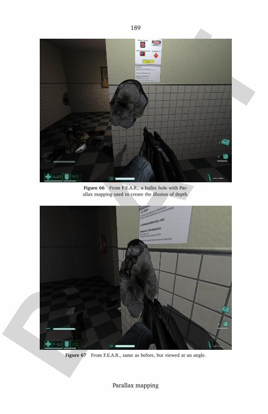
DRAF

T

189

Parallax mapping

Figure 66 From F.E.A.R., a bullet hole with Par-allax mapping used to create the illusion of depth.

Figure 67 From F.E.A.R., same as before, but viewed at an angle.

DRAF

T

190

Parallax mapping

Figure 68 From F.E.A.R., when viewed at an ex-treme angle, the illusion of depth disappears.

An easy way to understand this concept is to close one eye, take a pencil, pointit at your eye, and move your head left and right. Parallax mapping takes thatpixel on the far left of the pencil when it was facing you directly and stretchesit accordingly to simulate your angle in comparison to the pencil.

Parallax mapping is also a way of faking displacement mapping where the ac-tual geometric position of points surface is displaced along the surface normalaccording to the values stored into the texture: in Parallax mapping, like innormal and bump mapping, the silhouette of the object is unaffected.

See also

• Parallax

External links

• Detailed Shape Representation with Parallax Mapping237

• Parallax mapping implementation in DirectX, forum topic238

http://vrsj.t.u-tokyo.ac.jp/ic-at/ICAT2003/papers/01205.pdf237

http://www.gamedev.net/community/forums/topic.asp?topic_id=387447238

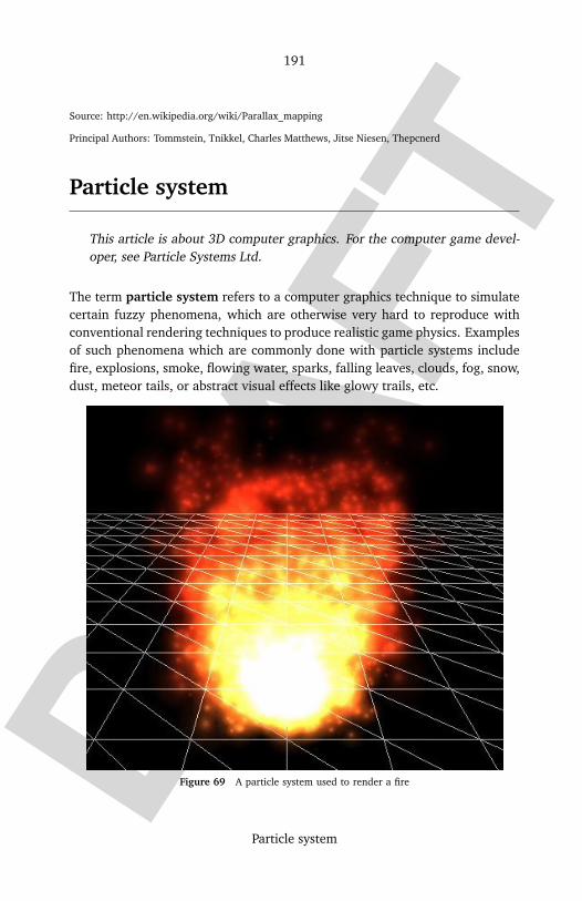
DRAF

T

191

Particle system

Source: http://en.wikipedia.org/wiki/Parallax_mapping

Principal Authors: Tommstein, Tnikkel, Charles Matthews, Jitse Niesen, Thepcnerd

Particle system

This article is about 3D computer graphics. For the computer game devel-oper, see Particle Systems Ltd.

The term particle system refers to a computer graphics technique to simulatecertain fuzzy phenomena, which are otherwise very hard to reproduce withconventional rendering techniques to produce realistic game physics. Examplesof such phenomena which are commonly done with particle systems includefire, explosions, smoke, flowing water, sparks, falling leaves, clouds, fog, snow,dust, meteor tails, or abstract visual effects like glowy trails, etc.

Figure 69 A particle system used to render a fire

DRAF

T

192

Particle system

Figure 70 A particle system used to render a galaxy

Figure 71 An abstract trail of particles

DRAF

T

193

Particle system

Typical implementationTypically the particle system’s position in 3D space or motion therein is con-trolled by what is called the emitter.

The emitter is mainly characterized by a set of particle behavior parametersand a position in 3D space. The particle behavior parameters might includespawning rate (how many particles are generated per unit of time), particleinitial velocity vector (i.e. which way will it go when it is emitted), particle life(how much time does each individual particle live before being extinguished),particle color and variations throughout its life, and many more. It is commonfor all or most of these parameters to be fuzzy, in the sense that instead of ab-solute values, some central value and allowable random variation is specified.

A typical particle system update loop (which is performed for each frameof animation) can be separated into two distinct stages, the parameter up-date/simulation stage and the rendering stage.

Simulation stageDuring the simulation stage, the amount of new particles that must be createdis calculated based on spawning rates and interval between updates, and eachof them is spawned in a specific position in 3D space based on emitter positionand spawning area specified. Also each of the particle’s parameters, like veloc-ity, color, life, etc, are initialized based on the emitter’s parameters. Then allthe existing particles are checked to see if they have exceeded their lifetime,in which case they are removed from the simulation. Otherwise their positionand other characteristics are modified based on some sort of physical simula-tion, which can be as simple as adding the velocity to the current position, andmaybe accounting for friction by modulating the velocity, or as complicated asperforming physically-accurate trajectory calculations taking into account ex-ternal forces. Also it is common to perform some sort of collision checking withspecified 3D objects in order to make the particles bounce off obstacles in theenvironment. However particle-particle collisions are rarely used, as they arecomputationally expensive and not really useful for most of the simulations.

A particle system has its own rules that are applied to every particle. Oftenthese rules involve interpolating values over the lifetime of a particle. Forexample, many systems have particles fade out to nothingness by interpolatingthe particle’s alpha value (opacity) during the lifetime of the particle.

Rendering stageAfter the update is complete, each particle is rendered usually in the formof a textured billboarded quad (i.e. a quadrilateral that is always facing the

DRAF

T

194

Path Tracing

viewer). However, this is not necessary, the particle may be rendered as justa single pixel in small resolution/limited processing power environments, oreven as a metaball in off-line rendering (isosurfaces computed from particle-metaballs make quite convincing liquid surfaces). Finally 3D meshes can alsobe used to render the particles.

Artist-friendly particle system toolsParticle systems can be created and modified natively in many 3D modelingand rendering packages including 3D Studio Max, Maya and Blender. Theseeditor programs allow artists to have instant feedback on how a particle sys-tem might look given properties and rules that they can specify. There is alsoplug-in software available that provide enhanced particle effects, such as After-Burn and RealFlow (for liquids). Compositing software such as Combustion orspecialized, particle-only software such as Particle Studio, can be used for thecreation of particle systems for film and video.

External links

• Particle Systems: A Technique for Modeling a Class of Fuzzy Objects239 –William T. Reeves (ACM Transactions on Graphics, April 1983)

Source: http://en.wikipedia.org/wiki/Particle_system

Principal Authors: Jtsiomb, Ashlux, Mrwojo, Sideris, The Merciful, MarSch

Path Tracing

Path tracing is a technique by James Kajiya when he presented his paper onthe Rendering Equation in the 1980s. The main goal of path tracing is to fullysolve the rendering equation.

A form of ray tracing whereby each ray is recursively traced along a path untilit reaches a light emitting source where the light contribution along the path iscalculated. This recursive tracing helps for solving the lighting equation moreaccurately than conventional ray tracing.

A simple path tracing pseudocode might look something like this:

http://portal.acm.org/citation.cfm?id=357320239

DRAF

T

195

Path Tracing

Color TracePath(Ray r,depth) if(depth==MaxDepth)

return Black; // bounced enough times

r.FindNearestObject();

if(r.hitSomething==false)

return Black; // nothing was hit

Material &m=r.thingHit->material;

Color emittance=m.emittance;

// pick a random direction from here and keep going

Ray newRay;

newRay.origin=r.pointWhereObjWasHit;

newRay.direction=RandomUnitVectorInHemisphereOf(r.normalWhereObjWasHit);

float cost=DotProduct(newRay.direction,r.normalWhereObjWasHit);

Color BRDF=m.reflectance/PI;

float scale=1.0*PI;

Color reflected=TracePath(newRay,depth+1);

return emittance + ( BRDF * scale * cost * reflected );

In the above example if every surface of a closed space emitted and reflected(0.5,0.5,0.5) then every pixel in the image would be white.

A variation of this algorithm is to trace rays in the opposite direction, fromlight sources to the camera, this is called light tracing. Furthermore these twoalgorithms can be combined to enhance the image results and which is calledbi-directional path tracing.

Source: http://en.wikipedia.org/wiki/Path_Tracing

Principal Authors: Icairns, RJHall

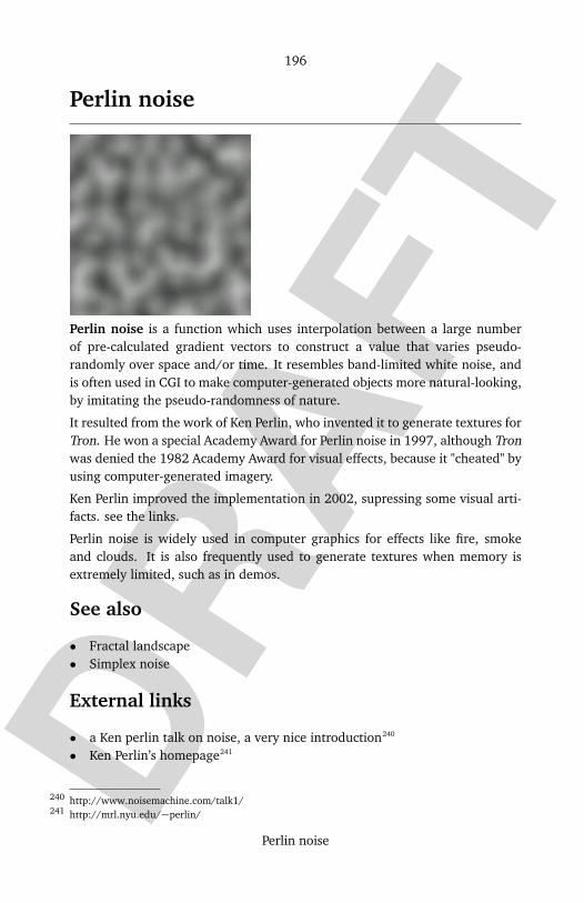
DRAF

T

196

Perlin noise

Perlin noise

Perlin noise is a function which uses interpolation between a large numberof pre-calculated gradient vectors to construct a value that varies pseudo-randomly over space and/or time. It resembles band-limited white noise, andis often used in CGI to make computer-generated objects more natural-looking,by imitating the pseudo-randomness of nature.

It resulted from the work of Ken Perlin, who invented it to generate textures forTron. He won a special Academy Award for Perlin noise in 1997, although Tronwas denied the 1982 Academy Award for visual effects, because it "cheated" byusing computer-generated imagery.

Ken Perlin improved the implementation in 2002, supressing some visual arti-facts. see the links.

Perlin noise is widely used in computer graphics for effects like fire, smokeand clouds. It is also frequently used to generate textures when memory isextremely limited, such as in demos.

See also

• Fractal landscape• Simplex noise

External links

• a Ken perlin talk on noise, a very nice introduction240

• Ken Perlin’s homepage241

http://www.noisemachine.com/talk1/240

http://mrl.nyu.edu/~perlin/241

DRAF

T

197

Per-pixel lighting

• Ken perlin’s improved noise (2002) java source code242

• Ken Perlin’s Academy Award page243

• Matt Zucker’s Perlin noise math FAQ244

• A very good explanation and implementation of Perlin noise, with pseudocode245

Source: http://en.wikipedia.org/wiki/Perlin_noise

Principal Authors: Michael Hardy, Charles Matthews, Reedbeta, Maa, Saga City, Gordmoo

Per-pixel lighting

In computer graphics, per-pixel lighting is commonly used to refer to a setof methods for computing illumination at each rendered pixel of an image.These generally produce more realistic images than vertex lighting, which onlycalculates illumination at each vertex of a →3D model and then interpolatesthe resulting values to calculate the per-pixel color values.

Per-pixel lighting is commonly used with other computer graphics techniquesto help improve render quality, including bump mapping, specularity, phongshading and shadow volumes.

Real-time applications, such as computer games, which use modern graph-ics cards will normally implement per-pixel lighting algorithms using pixelshaders. Per-pixel lighting is also performed on the CPU in many high-endcommercial rendering applications which typically do not render at interactiveframerates.

See also

• →Phong shading• Stencil shadow volumes• →Unified lighting and shadowing

Source: http://en.wikipedia.org/wiki/Per-pixel_lighting

http://mrl.nyu.edu/~perlin/noise/242

http://www.mrl.nyu.edu/~perlin/doc/oscar.html243

http://www.cs.cmu.edu/~mzucker/code/perlin-noise-math-faq.html244

http://freespace.virgin.net/hugo.elias/models/m_perlin.htm245

DRAF

T

198

Phong reflection model

Principal Authors: Mikkalai, Alphonze, Jheriko, David Wahler


Not to be confused with →Phong shading.

The Phong reflection model is an illumination and shading model, used in→3D computer graphics for assigning shades to points on a modeled surface.It was developed by →Bui Tuong Phong in his University of Utah Ph.D. disser-tation "Illumination for Computer Generated Pictures" in 1973, in conjunctionwith a method for interpolating the calculation for each individual pixel thatis rasterized from a polygonal surface model; the interpolation technique isknown as →Phong shading, even when it is used with a reflection model otherthan Phong’s.

The Phong reflection model can be treated as a simplification of the more gen-eral rendering equation; it takes advantage of the following simplificationswhen deciding the shade of a point on a surface:

1. It is a local reflection model, i.e. it doesn’t account for second-order reflec-tions, as do raytracing or radiosity. In order to compensate for the loss ofsome reflected light, an extra ambient lighting term is added to the scenethat is rendered.

2. It divides the reflection from a surface into three subcomponents, specularreflection, diffuse reflection, and ambient reflection.

If we first define, for each light source in the scene to be rendered, the com-ponents is and id, where these are the intensities (often as RGB values) ofthe specular and diffuse components of the light sources respectively. A singleia term controls the ambient lighting; it is sometimes computed as a sum ofcontributions from the light sources.

If we then define, for each material (which is typically assigned 1-to-1 for theobject surfaces in the scene):

ks: specular reflection constant, the ratio of reflection of the specular termof incoming light

kd: diffuse reflection constant, the ratio of reflection of the diffuse term ofincoming light

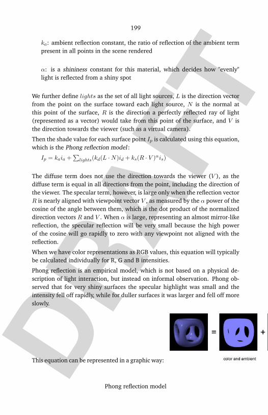
DRAF

T

199


ka: ambient reflection constant, the ratio of reflection of the ambient termpresent in all points in the scene rendered

α: is a shininess constant for this material, which decides how "evenly"light is reflected from a shiny spot

We further define lights as the set of all light sources, L is the direction vectorfrom the point on the surface toward each light source, N is the normal atthis point of the surface, R is the direction a perfectly reflected ray of light(represented as a vector) would take from this point of the surface, and V isthe direction towards the viewer (such as a virtual camera).

Then the shade value for each surface point Ip is calculated using this equation,which is the Phong reflection model :

Ip = kaia +∑

lights(kd(L ·N)id + ks(R · V )αis)

The diffuse term does not use the direction towards the viewer (V ), as thediffuse term is equal in all directions from the point, including the direction ofthe viewer. The specular term, however, is large only when the reflection vectorR is nearly aligned with viewpoint vector V , as measured by the α power of thecosine of the angle between them, which is the dot product of the normalizeddirection vectors R and V . When α is large, representing an almost mirror-likereflection, the specular reflection will be very small because the high powerof the cosine will go rapidly to zero with any viewpoint not aligned with thereflection.

When we have color representations as RGB values, this equation will typicallybe calculated individually for R, G and B intensities.

Phong reflection is an empirical model, which is not based on a physical de-scription of light interaction, but instead on informal observation. Phong ob-served that for very shiny surfaces the specular highlight was small and theintensity fell off rapidly, while for duller surfaces it was larger and fell off moreslowly.

This equation can be represented in a graphic way:

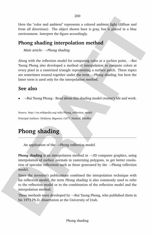
DRAF

T

200

Phong shading

Here the "color and ambient" represents a colored ambient light (diffuse andfrom all directions). The object shown here is gray, but is placed in a blueenvironment. Interpret the figure accordingly.

Phong shading interpolation methodMain article: →Phong shading

Along with the reflection model for computing color at a surface point, →BuiTuong Phong also developed a method of interpolation to compute colors atevery pixel in a rasterized triangle representing a surface patch. These topicsare sometimes treated together under the term →Phong shading, but here thelatter term is used only for the interpolation method.

See also

• →Bui Tuong Phong : Read about this shading model creator’s life and work.

Source: http://en.wikipedia.org/wiki/Phong_reflection_model

Principal Authors: Dicklyon, Bignoter, Csl77, Nixdorf, Srleffler

Phong shading

An application of the →Phong reflection model.

Phong shading is an interpolation method in →3D computer graphics, usinginterpolation of surface normals in rasterizing polygons, to get better resolu-tion of specular reflections such as those generated by the →Phong reflectionmodel.

Since the inventor’s publications combined the interpolation technique withhis reflection model, the term Phong shading is also commonly used to referto the reflection model or to the combination of the reflection model and theinterpolation method.

These methods were developed by →Bui Tuong Phong, who published them inhis 1973 Ph.D. dissertation at the University of Utah.

DRAF

T

201

Phong shading

Phong illumination or reflection modelMain article: →Phong reflection model

Phong reflection is a local illumination model that can produce a certain degreeof realism in three-dimensional objects by combining three elements: diffuse,specular, and ambient lighting for each considered point on a surface.

The reflection model has nothing specific to polygons or pixels, unlike the in-terpolation method.

Phong interpolation

Figure 72 Phong shading interpolation example

As a rendering method, Phong shading can be regarded as an improvement on→Gouraud shading that provides a better approximation to a point-by-pointapplication of an underlying reflection model by assuming a smoothly vary-ing surface normal vector. The Phong interpolation method works better thanGouraud shading when applied to the Phong reflection model or to any reflec-tion model that has small specular highlights.

The main problem with Gouraud shading is that when a specular highlightoccurs near the center of a large triangle, it will usually be missed entirely, dueto the interpolation of colors between vertices. This problem is fixed by Phongshading.

We are given three vertices in two dimensions, v 1, v 2 and v 3, as well as sur-face normals for each vertex n 1, n 2 and n 3; we assume these are of unit length.Unlike →Gouraud shading, which interpolates colors across triangles, in Phongshading we linearly interpolate a normal vector N across the surface of the tri-angle, from the three given normals. This is done for each pixel in the triangle,and at each pixel we normalize N and use it in the Phong illumination modelto obtain the final pixel color.

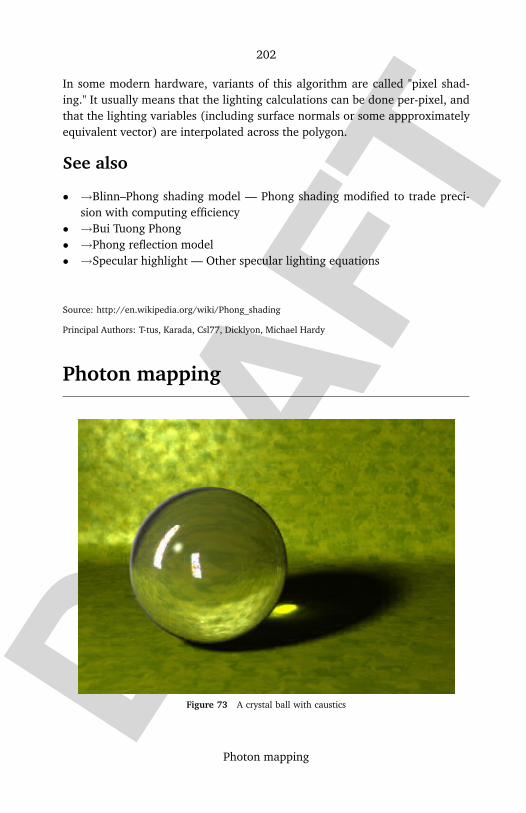
DRAF

T

202

Photon mapping

In some modern hardware, variants of this algorithm are called "pixel shad-ing." It usually means that the lighting calculations can be done per-pixel, andthat the lighting variables (including surface normals or some appproximatelyequivalent vector) are interpolated across the polygon.

See also

• →Blinn–Phong shading model — Phong shading modified to trade preci-sion with computing efficiency

• →Bui Tuong Phong• →Phong reflection model• →Specular highlight — Other specular lighting equations

Source: http://en.wikipedia.org/wiki/Phong_shading

Principal Authors: T-tus, Karada, Csl77, Dicklyon, Michael Hardy

Photon mapping

Figure 73 A crystal ball with caustics

DRAF

T

203

Photon mapping

In computer graphics, photon mapping is a global illumination algorithmbased on ray tracing used to realistically simulate the interaction of light withdifferent objects. Specifically, it is capable of simulating the refraction of lightthrough a transparent substance, such as glass or water, diffuse interreflectionsbetween illuminated objects, and some of the effects caused by particulate mat-ter such as smoke or water vapor. It was developed by Henrik Wann Jensen.

In the context of the refraction of light through a transparent medium, the de-sired effects are called caustics. A caustic is a pattern of light that is focused ona surface after having had the original path of light rays bent by an intermedi-ate surface. An example is a glass of wine on a table. As light rays pass throughthe glass and the liquid, they are refracted and focused on the table the glass isstanding on. The wine in the glass also produces interesting effects, changingthe pattern of light as well as its color.

With photon mapping, light packets (photons) are sent out into the scene fromthe light source. Whenever a photon intersects with a surface, the intersec-tion point, incoming direction, and energy of the photon are stored in a cachecalled the photon map. As each photon is bounced or refracted by intermedi-ate surfaces, the energy gets absorbed until no more is left. We can then stoptracing the path of the photon. Often we stop tracing the path after a prede-fined number of bounces in order to save time. One of the great advantagesof photon mapping is the independence of the scene’s description. That is, thescene can be modelled using any type of geometric primitive as for instancetriangles, spheres, etc.

Another technique is to send out groups of photons instead of individual pho-tons. In this case, each group of photons always has the same energy, thus thephoton map need not store energy. When a group intersects with a surface, itis either completely transmitted or completely absorbed. This is a Monte Carlomethod called Russian roulette.

To avoid emitting unneeded photons, the direction of the outgoing rays is oftenconstrained. Instead of simply sending out photons in random directions, theyare sent in the direction of a known object that we wish to use as a photon ma-nipulator to either focus or diffuse the light. There are many other refinementsthat can be made to the algorithm like deciding how many photons to send,and where and in what pattern to send them.

Photon mapping is generally a preprocess and is carried out before the mainrendering of the image. Often the photon map is stored on disk for later use.Once the actual rendering is started, every intersection of an object by a rayis tested to see if it is within a certain range of one or more stored photonsand if so, the energy of the photons is added to the energy calculated using a

DRAF

T

204

Photorealistic (Morph)

standard illumination equation. The slowest part of the algorithm is searchingthe photon map for the nearest photons to the point being illuminated.

The BRL-CAD ray tracer includes an open source implementation of photonmapping. Although photon mapping was designed to work primarily with raytracers, it can also be used with scanline renderers.

External links

• Realistic Image Synthesis Using Photon Mapping 246 ISBN 1568811470• Photon mapping introduction247 from Worcester Polytechnic Institute

• Global Illumination using Photon Maps - Henrik Wann Jensen 248

Source: http://en.wikipedia.org/wiki/Photon_mapping

Principal Authors: Flamurai, MichaelGensheimer, Curps, Phrood, Patrick, Brlcad, Fnielsen, Nilmerg

Photorealistic (Morph)

Photorealistic computer graphics can be created by taking an original 3D ren-dering, which resembles a photograph, and morphing the image in photoshop.This creates a life-like 3D model, using a real image, that is a time consumingchore for 3D animators.

An example of a photorealistic morph looks like this image below

http://graphics.ucsd.edu/~henrik/papers/book/246

http://www.cs.wpi.edu/~emmanuel/courses/cs563/write_ups/zackw/photon_mapping/PhotonMap-247

ping.htmlhttp://graphics.ucsd.edu/~henrik/papers/ewr7/egwr96.pdf248

DRAF

T

205

PLIB

See also

• 3D Rendering• photoshopping

Source: http://en.wikipedia.org/wiki/Photorealistic_%28Morph%29

PLIB

PLIB is a suite of Open Sourced portable computer game libraries, originallywritten by Steve Baker in 1997 and licensed under the LGPL.

PLIB includes sound effects, music, a complete 3D engine, font rendering, asimple windowing library, a game scripting language, a GUI, networking, 3Dmath library and a collection of utility functions. All are 100% portable acrossnearly all modern computing platforms. Each library component is fairly in-dependent of the others - so if you want to use SDL, GTK+, GLUT, or FLTKinstead of PLIB’s ’PW’ windowing library, you can.

PLIB is used by many projects (not all games - and not all OpenSourced).

See also

• Allegro• OpenML• Simple DirectMedia Layer• DirectX• →OpenGL• ClanLib

External links

• PLIB website249

Source: http://en.wikipedia.org/wiki/PLIB

http://plib.sourceforge.net/249

DRAF

T

206

Polygonal modeling

Polygonal modeling

In →3D computer graphics, polygonal modeling is an approach for modelingobjects by representing or approximating their surfaces using polygons. Polyg-onal modeling is well suited to scanline rendering and is therefore the methodof choice for real-time computer graphics. Alternate methods of representing3D objects include NURBS surfaces, subdivision surfaces, and equation-basedrepresentations used in ray tracers.

Geometric Theory and PolygonsThe basic object used in mesh modeling is a vertex, a point in three dimen-sional space. Two vertices connected by a straight line become an edge. Threevertices, connected to the each other by three edges, define a triangle, whichis the simplest polygon in Euclidean space. More complex polygons can be cre-ated out of multiple triangles, or as a single object with more than 3 vertices.Four sided polygons (generally referred to as quads) and triangles are the mostcommon shapes used in polygonal modeling. A group of polygons, connectedto each other by shared vertices, is generally referred to as an element. Eachof the polygons making up an element is called a face.

In Euclidean geometry, any three points determine a plane. For this reason,triangles always inhabit a single plane. This is not necessarily true of morecomplex polygons, however. The flat nature of triangles makes it simple to de-termine their surface normal, a three-dimensional vector perpendicular to thetriangle’s edges. Surface normals are useful for determining light transport inray tracing, and are a key component of the popular →Phong shading model.Some rendering systems use vertex normals instead of surface normals to cre-ate a better-looking lighting system at the cost of more processing. Note thatevery triangle has two surface normals, which face away from each other. Inmany systems only one of these normals is considered valid – the other side ofthe polygon is referred to as a backface, and can be made visible or invisibledepending on the programmer’s desires.

Many modeling programs do not strictly enforce geometric theory; for exam-ple, it is possible for two vertices to have two distinct edges connecting them,occupying the exact same spatial location. It is also possible for two vertices toexist at the same spatial coordinates, or two faces to exist at the same location.Situations such as these are usually not desired by the user, and must be fixedmanually.

DRAF

T

207

Polygonal modeling

A group of polygons which are connected together by shared vertices is referredto as a mesh. In order for a mesh to appear attractive when rendered, it is de-sirable that it be non-self-intersecting, meaning that no edge passes through apolygon. Another way of looking at this is that the mesh cannot pierce itself. Itis also desirable that the mesh not contain any errors such as doubled vertices,edges, or faces. For some purposes it is important that the mesh be a manifold– that is, that it does not contain holes or singularities (locations where twodistinct sections of the mesh are connected by a single vertex).

Construction of Polygonal MeshesAlthough it is possible to construct a mesh by manually specifying vertices andfaces, it is much more common to build meshes using a variety of tools. A widevariety of 3d graphics software packages are available for use in constructingpolygon meshes.

One of the more popular methods of constructing meshes is box modeling,which uses two simple tools:

• The subdivide tool splits faces and edges into smaller pieces by adding newvertices. For example, a square would be subdivided by adding one vertexin the center and one on each edge, creating four smaller squares.

• The extrude tool is applied to a face or a group of faces. It creates a newface of the same size and shape which is connected to each of the existingedges by a face. Thus, performing the extrude operation on a square facewould create a cube connected to the surface at the location of the face.

A second common modeling method is sometimes referred to as inflation mod-eling or extrusion modeling. In this method, the user creates a 2d shapewhich traces the outline of an object from a photograph or a drawing. The us-er then uses a second image of the subject from a different angle and extrudesthe 2d shape into 3d, again following the shape’s outline. This method is es-pecially common for creating faces and heads. In general, the artist will modelhalf of the head and then duplicate the vertices, invert their location relative tosome plane, and connect the two pieces together. This ensures that the modelwill be symmetrical.

Another common method of creating a polygonal mesh is by connecting to-gether various primitives, which are predefined polygonal meshes created bythe modeling environment. Common primitives include:

• Cubes• Pyramids

DRAF

T

208

Polygonal modeling

• Cylinders• 2D primitives, such as squares, triangles, and disks• Specialized or esoteric primitives, such as the Utah Teapot or Suzanne,

Blender’s monkey mascot.• Spheres - Spheres are commonly represented in one of two ways:

• Icospheres are icosahedrons which possess a sufficient number of tri-angles to resemble a sphere.

• UV Spheres are composed of quads, and resemble the grid seen on someglobes - quads are larger near the "equator" of the sphere and smallernear the "poles," eventually terminating in a single vertex.

Finally, some specialized methods of constructing high or low detail meshesexist. Sketch based modeling is a user-friendly interface for constructing low-detail models quickly, while 3d scanners can be used to create high detail mesh-es based on existing real-world objects in almost automatic way. These devicesare very expensive, and are generally only used by researchers and industryprofessionals but can generate high accuracy sub-millimetric digital represen-tations.

ExtensionsOnce a polygonal mesh has been constructed, further steps must be taken be-fore it is useful for games, animation, etc. The model must be texture mappedto add colors and texture to the surface and it must be given an inverse kine-matics skeleton for animation. Meshes can also be assigned weights and cen-ters of gravity for use in physical simulation.

In order to display a model on a computer screen outside of the modelingenvironment, it is necessary to store that model in one of the file formats listedbelow, and then use or write a program capable of loading from that format.The two main methods of displaying 3d polygon models are →OpenGL and→Direct3D. Both of these methods can be used with or without a graphicscard.

Advantages and disadvantagesThere are many disadvantages to representing an object using polygons. Poly-gons are incapable of accurately representing curved surfaces, so a large num-ber of them must be used to approximate curves in a visually appealing manner.The use of complex models has a cost in lowered speed. In scanline conver-sion, each polygon must be converted and displayed, regardless of size, andthere are frequently a large number of models on the screen at any given time.

DRAF

T

209

Polygonal modeling

Often, programmers must use multiple models at varying levels of detail to rep-resent the same object in order to cut down on the number of polygons beingrendered.

The main advantage of polygons is that they are faster than other represen-tations. While a modern graphics card can show a highly detailed scene at aframe rate of 60 frames per second or higher, raytracers, the main way of dis-playing non-polygonal models, are incapable of achieving an interactive framerate (10 fps or higher) with a similar amount of detail.

File FormatsA variety of formats are available for storing 3d polygon data. The most popu-lar are:

• .3ds, .max, which is associated with 3D Studio Max• .mb and .ma, which are associated with Maya• .lwo, which is associated with Lightwave• .obj (Wavefront’s "The Adanced Visualizer")• .C4d associated with Cinema 4D• .dxf, .dwg, .dwf, associated with AutoCAD• .md3, .md2, associated with the Quake series of games• .fbx (Alias)• .rwx (Renderware)• .wrl (VRML 2.0)

External links

• Free models in a variety of formats: 3dcafe250

• Computer graphics latest news, reviews, tutorials and interviews:InsideCG251

• Computer graphics news: CG Channel252

• Computer graphics forums, reviews, and contests: CG Society253

• Open Source 3d modeling program: Blender 254

• Simple, small and open source 3D modelling program: Wings 3D 255

• Open Source 3D modeling program: AutoQ3D 256

http://www.3dcafe.com/250

http://www.insidecg.com/251

http://www.cgchannel.com/252

http://www.cgsociety.org/253

http://www.blender.org/254

http://www.Wings3D.com/255

http://autoq3d.ecuadra.com/256

DRAF

T

210

Polygon (computer graphics)

ReferencesOpenGL SuperBible (3rd ed.), by Richard S Wright and Benjamin Lipchak ISBN0672326019

OpenGL Programming Guide: The Official Guide to Learning OpenGL, Version1.4, Fourth Edition by OpenGL Architecture Review Board ISBN 0321173481

OpenGL(R) Reference Manual : The Official Reference Document to OpenGL,Version 1.4 (4th Edition) by OpenGL Architecture Review Board ISBN032117383X

Blender documentation: http://www.blender.org/cms/Documentation.628.0.html

Maya documentation: packaged with Alias Maya, http://www.alias.com/eng/index.shtml

See also

• Finite element analysis / method• →Polygon mesh• Vector graphics

Source: http://en.wikipedia.org/wiki/Polygonal_modeling

Principal Authors: Furrykef, Jreynaga, KenArthur, Peter L, TenOfAllTrades, RJFJR

Polygon (computer graphics)

Polygons are used in computer graphics to compose images that are three-dimensional in appearance. Usually (but not always) triangular, polygons arisewhen an object’s surface is modeled, vertices are selected, and the object isrendered in a wire frame model. This is quicker to display than a shadedmodel; thus the polygons are a stage in computer animation. The polygoncount refers to the number of polygons being rendered per frame.

Competing methods for rendering polygons thatavoid seams

• point

DRAF

T

211

Polygon mesh

• floating point• Fixed-point• polygon• because of rounding, every scanline has its own direction in space and

may show its front or back side to the viewer.• Fraction (mathematics)

• Bresenham’s line algorithm• polygons have to be split into triangles• the whole triangle shows the same side to the viewer• the point numbers from the →Transform and lighting stage have to con-

verted to Fraction (mathematics)• Barycentric coordinates (mathematics)

• used in raytracing

See also

• Polygon, for general polygon information• →Polygon mesh, for polygon object representation• Polygon modeling

Source: http://en.wikipedia.org/wiki/Polygon_%28computer_graphics%29

Principal Authors: Michael Hardy, Arnero, Orderud, SimonP, BlazeHedgehog

Polygon mesh

A polygon mesh is a collection of vertices and polygons that define the shapeof an object in →3D computer graphics.

Meshes usually consists of triangles, quadrilaterals or other simple convex poly-gons, since this simplifies rendering, but they can also contain objects made ofgeneral polygons with optional holes.

Examples of internal mesh structure representations:

• Simple list of vertices with a list of indices describing which vertices arelinked to form polygons; additional information can describe a list of holes

• List of vertices + list of edges (pairs of indices) + list of polygons that linkedges

• Winged edge data structure

DRAF

T

212

Precomputed Radiance Transfer

The choice of the data structure is governed by the application: it’s easier todeal with triangles than general polygons, especially in computational geome-try. For optimized algorithms it is necessary to have a fast access to topologicalinformations such as edges or neighbouring faces; this requires more complexstructures such as the winged-edge representation.

Source: http://en.wikipedia.org/wiki/Polygon_mesh

Principal Authors: Orderud, Furrykef

Precomputed Radiance Transfer

Precomputed Radiance Transfer (PRT) is a technique used to render a scenein real time with complex light interactions precomputed. →Radiosity canbe used to determine the diffuse lighting of the scene, however PRT offers amethod to dynamically change the lighting environment.

In essense, PRT computes the illumination of a point as a linear combinationof incident irradiance. An efficient method must be used to encode this data,such as Spherical harmonics.

Reference: Sloan, Peter-Pike, Jan Kautz, and John Snyder. "Precomputed Ra-diance Transfer for Real-Time Rendering in Dynamic, Low-Frequency LightingEnvironments". ACM Transactions on Graphics, Proceedings of the 29th Annu-al Conference on Computer Graphics and Interactive Techniques (SIGGRAPH),pp. 527-536. New York, NY: ACM Press, 2002.

Source: http://en.wikipedia.org/wiki/Precomputed_Radiance_Transfer

Principal Authors: Bhouston

DRAF

T

213

Procedural generation

Pre-rendered

Pre-rendered graphics, in computer graphics, is a video footage which is notbeing rendered in real-time by the hardware that is outputing or playing backthe video. Instead, the video is a recording of a footage that was previouslyrendered on a different equipment (typically one that is more powerful thanthe hardware used for playback). The advantage of pre-rendering is the abilityto use graphic models that are more complex and computationally intensivethan what can be rendered in real-time, due to the possibility of using multiplecomputers over extended periods of time to render the end results. The dis-advantage of pre-rendering, in the case of video game graphics, is a generallylower level of interactivity, if any, with the player.

CG movies such as Toy Story, Shrek and Final Fantasy: The Spirits Within areentirely pre-rendered. Pre-rendered graphics are used primarily as cut scenesin modern video games, where they are also known as full motion video.

See also

• →Rendering (computer graphics)• FMV game

Source: http://en.wikipedia.org/wiki/Pre-rendered


Procedural generation is a widely used term to indicate the possibility to cre-ate content on the fly, as opposed to creating it before distribution. This is oftenrelated to computer graphics applications.

Procedural synthesis is actually the correct term for this kind of approach, re-calling as "electronic sounds" have been (and still are) generated by synthe-sizers from nothing but electricity and user’s creativity.[citation needed ] In thisdocument, the terms "synthesis" and "generation" are used interchangeably.

More generally, the term ’procedural’ is strictly related to a procedure used tocompute particular functions. This concept is similar to a fractal, although thelatter is considered to be much more math-involved. Most common procedu-rally generated content include textures and meshes. Sound is seldom proce-durally generated in PC applications. While procedural generation techniques

DRAF

T

214


have been employed for years in countless games, few actually used this ap-proach extensively. The exception is Will Wright’s Spore, a highly-anticipatedvideo game title populated entirely with procedurally generated content. Some"procedurally generated" elements also appeared in previous games: the firstSoldier of Fortune from Raven Software used simple routines to add randomdetail to enemy models. To a certain degree, it could be said that the lightingin Doom 3 from id Software is "procedurally generated" because it does notrely on lightmaps precomputed using a radiosity process.

The modern demoscene uses procedural generation for squeezing a lot of im-pressive audiovisual content into very small executable programs. Farbrauschis a team famous for its achievements in this area, although many similar tech-niques were already implemented by The Black Lotus in the 1990’s.

Procedural generation as an application of func-tional programmingProcedurally generated content such as textures and landscapes may exhibitvariation, but the generation of a particular item or landscape must be identicalfrom frame to frame. Accordingly, the functions used must be referentiallytransparent, always returning the same result for the same point, so that theymay be called in any order and their results freely cached as necessary. This issimilar to lazy evaluation in functional programming languages.

Procedural generation in video gamesThe earliest computer games were severely limited by memory constraints.This forced content like maps to be generated algorithmically on the fly: theresimply wasn’t enough space to store premade levels and artwork. Today, mostgames include thousands of times as much data in terms of memory as algo-rithmic mechanics. For example, all of the buildings in the large gameworld ofGrand Theft Auto were individually designed and placed by artists.

In a typical modern video game, game content such as textures and characterand environment models are created by artists beforehand, then rendered inthe game engine. As the technical capabilities of computers and video gameconsoles increases, the amount of work required by artists also increases. First,high-end gaming PCs and next-generation game consoles like the Xbox 360and PlayStation 3 are capable of rendering scenes containing many very de-tailed objects with high-resolution textures in high-definition. This means thatartists must invest a great deal more time in creating a single character, vehicle,building, or texture, since gamers will tend to expect ever-increasingly detailedenvironments.

DRAF

T

215


Secondly, the number of unique objects displayed in a video game is increas-ing. In addition to highly detailed models, players expect a variety of modelsthat appear substantially different from one another. In older games, a singlecharacter or object model might have been used over and over again through-out a game. With the increased visual fidelity of modern games, however, it isvery jarring (and threatens the suspension of disbelief) to see many copies ofa single object, while the real world contains far more variety. Again, artistswould be required to complete orders of magnitude more work in order to cre-ate many different varieties of a particular object. The need to hire larger artstaffs is one of the reasons for skyrocketing game development budgets.

Some initial approaches to procedural synthesis attempted to solve these prob-lems by shifting the burden of content generation from the artists to program-mers who can create code which automatically generates different meshes ac-cording to input parameters. Although sometimes this still happens, what hasbeen recognized is that applying a purely procedural model is often hard atbest, requiring huge amounts of time to evolve into a functional, usable andrealistic-looking method. Instead of writing a procedure that completely buildscontent procedurally, it has been proven to be much cheaper and more effectiveto rely on artist created content for some details. For example, SpeedTree isa middleware used to generate trees procedurally with a large variety yet leaftextures can be fetched from regular files often representing digitally acquiredreal foliage. Other effective methods to generate hybrid content is to procedu-rally merge different pre-made assets or to procedurally apply some distortionsto them.

Supposing, however, a single algorithm can be envisioned to generate arealistic-looking tree, the algorithm could be called to generate random trees,thus filling a whole forest at runtime, instead of storing all the vertices requiredby the various models. This would save storage media space and reduce theburden on artist, while providing richer experience. The same method wouldrequire far more processing power in respect to a mere disk loading, but withCPUs getting faster, the problem is gradually becoming smaller. Please note,developing such algorithm is non-trivial for a single tree, let alone for a varietyof species (compare Sumac, Birch, Maple and its species), moreover assemblinga forest could not be done by just assembling trees because in real world thisintroduces interactions between the various trees which dramatically changetheir appearance (although this is probably a minor detail).

In 2004, a PC first-person shooter called .kkrieger was released that madeheavy use of procedural synthesis: while quite short and very simple, the ad-vanced video effects were packed into just 96 Kilobytes. In contrast, manymodern games are released across several CDs, often exceeding 2 gigabytes in

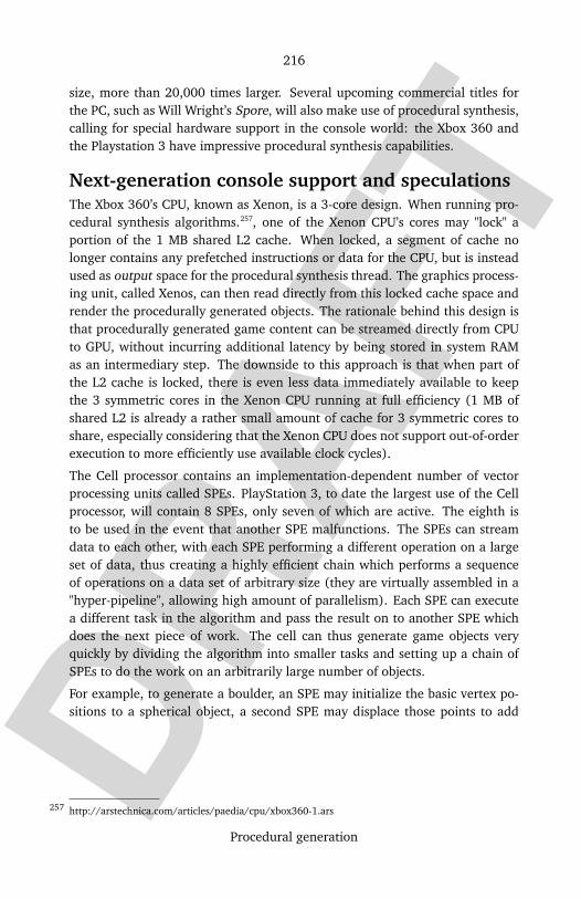
DRAF

T

216


size, more than 20,000 times larger. Several upcoming commercial titles forthe PC, such as Will Wright’s Spore, will also make use of procedural synthesis,calling for special hardware support in the console world: the Xbox 360 andthe Playstation 3 have impressive procedural synthesis capabilities.

Next-generation console support and speculationsThe Xbox 360’s CPU, known as Xenon, is a 3-core design. When running pro-cedural synthesis algorithms.257, one of the Xenon CPU’s cores may "lock" aportion of the 1 MB shared L2 cache. When locked, a segment of cache nolonger contains any prefetched instructions or data for the CPU, but is insteadused as output space for the procedural synthesis thread. The graphics process-ing unit, called Xenos, can then read directly from this locked cache space andrender the procedurally generated objects. The rationale behind this design isthat procedurally generated game content can be streamed directly from CPUto GPU, without incurring additional latency by being stored in system RAMas an intermediary step. The downside to this approach is that when part ofthe L2 cache is locked, there is even less data immediately available to keepthe 3 symmetric cores in the Xenon CPU running at full efficiency (1 MB ofshared L2 is already a rather small amount of cache for 3 symmetric cores toshare, especially considering that the Xenon CPU does not support out-of-orderexecution to more efficiently use available clock cycles).

The Cell processor contains an implementation-dependent number of vectorprocessing units called SPEs. PlayStation 3, to date the largest use of the Cellprocessor, will contain 8 SPEs, only seven of which are active. The eighth isto be used in the event that another SPE malfunctions. The SPEs can streamdata to each other, with each SPE performing a different operation on a largeset of data, thus creating a highly efficient chain which performs a sequenceof operations on a data set of arbitrary size (they are virtually assembled in a"hyper-pipeline", allowing high amount of parallelism). Each SPE can executea different task in the algorithm and pass the result on to another SPE whichdoes the next piece of work. The cell can thus generate game objects veryquickly by dividing the algorithm into smaller tasks and setting up a chain ofSPEs to do the work on an arbitrarily large number of objects.

For example, to generate a boulder, an SPE may initialize the basic vertex po-sitions to a spherical object, a second SPE may displace those points to add

http://arstechnica.com/articles/paedia/cpu/xbox360-1.ars257

DRAF

T

217


randomness, a third to generate normals, tangent and binormals for bumpmap-ping while a fourth SPE may add volume texture coordinates (possibly in paral-lel with the third SPE). Note that this example assumes the compiler can guesscorrect parallelism opportunity.

The Cell’s counterpart to Xenon "cache locking" is each SPE’s 256 KiB localstore, essentially L2 cache memory which can be accessed directly, rather thanbeing used to speed up access to main memory. This approach has both perksand flaws, as it allows each SPE to work extremely quickly, but only on a smallsubset of the total data of a program. There is also a direct 35 GB/s linkbetween the Cell and the PS3’s "Reality Synthesizer" GPU, allowing objects tobe sent directly to the GPU to be rendered as soon as they are generated.

See also

• →Procedural texture• Procedural animation• Fractal landscape• L-System

Software using procedural generation

• Elite (everything about the universe - planet positions, names, politics andgeneral descriptions - is generated procedurally; Ian Bell has released thealgorithms in C as text elite258)

• Exile• Frontier: Elite 2• Noctis• StarFlight• The Sentinel (computer game)• Most Roguelikes procedurally generate gameworlds.• Dozens of demos procedurally generate complex textures, sounds and 3D

objects.• SpeedTree is a widely known middleware to procedurally generate trees at

various levels in the production pipeline or at runtime using L-systems.• The Elder Scrolls IV: Oblivion• Many games using the upcoming Unreal Engine 3.

• Spore• Jade Cocoon (The merged minions were procedurally generated based on

body part sizes)

http://www.iancgbell.clara.net/elite/text/index.htm258

DRAF

T

218

Procedural texture

External links

• Real-time procedural generation of ‘pseudo infinite’ cities259 - ACM• The Future Of Content260 - Will Wright keynote on Spore & procedural gen-

eration at the Game Developers Conference 2005. (Scroll down 3/4 ofpage, registration required to view video).

• Procedural 3D Content Generation261 - Dean Macri and Kin Pallister - Intel- An excellent two-part article with an accompanying demo (including fullC++ source code).

• Darwinia262 - development diary263 procedural generation of terrains andtrees.

Source: http://en.wikipedia.org/wiki/Procedural_generation

Principal Authors: Jacoplane, MaxDZ8, Ashley Y, Viznut, Lapinmies, Tlogmer, Praetor alpha, Jess-

martin, ChopMonkey, Lupin

Procedural texture

A procedural texture is a computer generated image created using an algo-rithm intended to create a realistic representation of natural elements such aswood, marble, granite, metal, stone, and others.

Usually, the natural look of the rendered result is achieved by the usage offractal noise and turbulence functions. These functions are used as a numericalrepresentation of the “randomness” found in everything that surrounds us.

In general, these noise and fractal functions are simply used to “disturb” thetexture in a natural way such as the undulations of the veins of the wood. Inother cases, like marbles’ textures, they are based on the graphical representa-tion of fractal noise.


http://www.pqhp.com/cmp/gdctv/260

http://www.intel.com/cd/ids/developer/asmo-na/eng/20247.htm261

http://www.darwinia.co.uk/262

http://www.darwinia.co.uk/extras/development.html263

http://www.spiralgraphics.biz/gallery.htm264

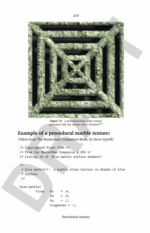
DRAF

T

219

Procedural texture

Figure 74 A procedural floor grate texturegenerated with the texture editor Genetica264.

Example of a procedural marble texture:(Taken from The Renderman Companion Book, by Steve Upstill)

/* Copyrighted Pixar 1988 */

/* From the RenderMan Companion p.355 */

/* Listing 16.19 Blue marble surface shader*/

/*

* blue marble(): a marble stone texture in shades of blue

* surface

*/

blue marble(

float Ks = .4,

Kd = .6,

Ka = .1,

roughness = .1,

DRAF

T

220

Procedural texture

txtscale = 1;

color specularcolor = 1)

point PP; /* scaled point in shader space */

float csp; /* color spline parameter */

point Nf; /* forward-facing normal */

point V; /* for specular() */

float pixelsize, twice, scale, weight, turbulence;

/* Obtain a forward-facing normal for lighting calculations.

*/

Nf = faceforward( normalize(N), I);

V = normalize(-I);

/*

* Compute "turbulence" a la [PERLIN85]. Turbulence is a sum

of

* "noise" components with a "fractal" 1/f power spectrum.

It gives the

* visual impression of turbulent fluid flow (for example, as

in the

* formation of blue marble from molten color splines!). Use

the

* surface element area in texture space to control the num-

ber of

* noise components so that the frequency content is appro-

priate

* to the scale. This prevents aliasing of the texture.

*/

PP = transform("shader", P) * txtscale;

pixelsize = sqrt(area(PP));

twice = 2 * pixelsize;

turbulence = 0;

for (scale = 1; scale > twice; scale /= 2)

turbulence += scale * noise(PP/scale);

/* Gradual fade out of highest-frequency component near limit

*/

if (scale > pixelsize) weight = (scale / pixelsize) - 1;

weight = clamp(weight, 0, 1);

DRAF

T

221

Procedural texture

turbulence += weight * scale * noise(PP/scale);

/*

* Magnify the upper part of the turbulence range 0.75:1

* to fill the range 0:1 and use it as the parameter of

* a color spline through various shades of blue.

*/

csp = clamp(4 * turbulence - 3, 0, 1);

Ci = color spline(csp,

color (0.25, 0.25, 0.35), /* pale blue */

color (0.25, 0.25, 0.35), /* pale blue */

color (0.20, 0.20, 0.30), /* medium blue */



color (0.25, 0.25, 0.35), /* pale blue */

color (0.25, 0.25, 0.35), /* pale blue */

color (0.15, 0.15, 0.26), /* medium dark blue */

color (0.15, 0.15, 0.26), /* medium dark blue */

color (0.10, 0.10, 0.20), /* dark blue */

color (0.10, 0.10, 0.20), /* dark blue */

color (0.25, 0.25, 0.35), /* pale blue */

color (0.10, 0.10, 0.20) /* dark blue */

);

/* Multiply this color by the diffusely reflected light. */

Ci *= Ka*ambient() + Kd*diffuse(Nf);

/* Adjust for opacity. */

Oi = Os;

Ci = Ci * Oi;

/* Add in specular highlights. */

Ci += specularcolor * Ks * specular(Nf,V,roughness);

This article was taken from The Photoshop Roadmap265 with written authoriza-tion

http://www.photoshoproadmap.com265

DRAF

T

222

Qualitative invisibility

See also

• →Perlin noise• →Procedural generation

Source: http://en.wikipedia.org/wiki/Procedural_texture

Principal Authors: MaxDZ8, Wikedit, TimBentley, Volfy, Viznut

Pyramid of vision

Pyramid of vision is a →3D computer graphics term: the infinite pyramid intothe real world, with an apex at the observer’s eye and faces passing throughthe edges of the viewport ("window").

Source: http://en.wikipedia.org/wiki/Pyramid_of_vision

Qualitative invisibility

In CAD/CAM, Qualitative Invisibility (QI) is the number of solid bodies ob-scuring a point in space as projected onto a plane (called [vector] hidden lineremoval used by the Vector format). Oftentimes, when a CAD engineer cre-ates a projection of his model into a plane [the drawing], he wishes to denotethe edges which are visible by a solid segment and those which are hiddenby dashed or dimmed segments. The idea of keeping track of the number ofobscuring bodies gives rise to an algorithm which propages the quantitative in-visibility throughout the model. This technique uses edge coherence to speedup the calculations in the algorithm. However, QI really only works well whenbodies are larger solids, non-interpenetrating, and not transparent. A tech-nique like this would fall apart when trying to render soft organic tissue asfound in the human body, because there is not always a clear delineation ofstructures. Also, when images become too cluttered and intertwined, then thecontribution of this algorithm is marginal.

Qualitative Invisibility is a term coined by Arthur Appel of the graphics groupat IBM Watson Research and used in several of his papers.

DRAF

T

223

Quaternions and spatial rotation

External link

• Vector Hidden Line Removal and Fractional Quantitative Invisibility266

ReferenceAppel, A., "The Notion of Quantitative Invisibility and the Machine Renderingof Solids," Proceedings ACM National Conference, Thompson Books, Washing-ton, DC, 1967, pp. 387-393, pp. 214-220.

Source: http://en.wikipedia.org/wiki/Qualitative_invisibility

Principal Authors: Wheger, Ulayiti, Patrick, Frencheigh


The main article on quaternions describes the history and purely mathe-matical properties of the algebra of quaternions. The focus of this article isthe practical application of these mathematical ideas in engineered physicalsystems.

The algebra of quaternions is a useful mathematical tool for formulating thecomposition of arbitrary spatial rotations, and establishing the correctness ofalgorithms founded upon such compositions. These methods find broad appli-cation in computer generated graphics, robotics, global navigation, and thespatial orientation of instruments. (citation: Quaternions and rotation Se-quences: a Primer with Applications to Orbits, Aerospace, and Virtual Reality,Kuipers, Jack B., Princeton University Press copyright 1999)

Familiarity with the definition of a quaternion and the associated arithmeticalrudiments is assumed. These may be gleaned from a cursory examination of afew paragraphs in the article on quaternions.

IntroductionThe 1909 edition of Webster’s unabridged dictionary (citation: Webster’s NewInternational Dictionary, G. & C. Merriam Co. copyright 1909, pp1752) definesa quaternion as

http://wheger.tripod.com/vhl/vhl.htm266

DRAF

T

224


5. Math. The quotient of two vectors ... Such is the view of the inventor,Sir Wm. Rowan Hamilton, and his disciple, Prof. P. G. Tait; but authoritiesare not yet quite agreed as to what a quaternion is or ought to be.

This definition together with the excised "..." is technically correct if the defini-tion of "vector" is restricted to its three dimensional conception, but the wag-gish remark serves to anecdotally illustrate the aura of arcane and possiblyirrational esotericism that encumbered the mathematical discipline in its earlydays. To some degree, the disrepute of those early perceptions persist today.

The purpose of this introduction is to demystify the quaternions by demon-strating that the underlying concepts are pervasive in the everyday experienceof ordinary people. This will establish a solid intuitive foundation upon whichthe mathematical and algorithmic content of the remainder of the article maybe constructed. In fact, when approached from a geometric perspective, thequaternion algebra is as easy to understand, utilize, and apply as the algebraof complex numbers.

Non-commutativityWhen considered as a purely numerical algebraic system, the non-commutativity of quaternion multiplication strikes many initiates as capriciousand counter-intuitive. The following simple exercise demonstrates otherwise.

Consider an asymmetrical object, for example, a book. Set it on a table so thatthe spine is to the left and the front cover is visible with the title readable.Define the three orthonormal spatial axes as follows: positive z extends upfrom the table, and x and y oriented as usual, i.e. x extending from left toright, and y extending away from the viewer.

The application of two rotation operators to the book will demonstrate non-commutativity. First, rotate the book 90 degrees clockwise about the z axis,so that the spine is facing away. Next rotate the book 180 degrees clockwiseabout the y axis, so that now the front cover faces down and the spine facesaway.

The application of these same two rotation operators in reverse order, firstyields the book in a position with the cover facing down and spine facing right.After applying the z rotation, the book rests in its final position with the coverfacing down and the spine facing forward, demonstrating zy 6=yz. In fact, thecomposition zy represents a single rotation of 180 degrees about the [-1 1 0]axis, and yz represents a single rotation of 180 degrees about the [1 1 0] axis.

In general, the composition of two different rotations about two distinct spatialaxes will not commute. This is a truth that all of us subconsciously understand

DRAF

T

225


and apply every day. Quaternion algebra is simply a mathematical formulationof this truth.

Double coveringThis second exercise demonstrates the property of a quaternion rotation op-erator that for each complete turn of the angular parameter, the image of theobject to which the operator is applied turns twice.

In a sitting position extend the forearm from the waist with the palm open andup. Place a small object, such as a coin on the open palm, so that only gravityholds the coin in the palm. When this exercise is complete, the palm (and coin)will have rotated 720 degrees or two turns, without dropping or squeezing thecoin.

Define the three orthonormal spatial axes as follows: positive z extends upfrom the palm, and x and y oriented as usual, i.e. x extending from left toright through the shoulder sockets, and y extending away from the viewer.

Four pivot axes are of interest. The first is attached to the shoulder socket andaligned with the y axis. The second is attached to the elbow, and is alignedorthogonal to the upper arm and forearm. The third is aligned with the fore-arm, and the fourth is aligned orthogonal to this at the wrist in the plane of thepalm.

First rotate the palm clockwise 180 degrees (counter-clockwise for left handedpeople). The various pivot axes will turn in synchrony in order to maintainthe palm facing up, so that the palm comes to rest over the shoulder with thefingers pointing back. Next rotate the palm another 180 degrees clockwise,with the gimbals modulating so that the palm comes to rest with the fingerspointing forward and the upper arm extended upward with the forearm angledup.

Similarly, continue with another 180 degrees, so that the palm lingers with thefingers pointing back under the armpit with the elbow akimbo up and backwith the upper arm extended horizontally. Finally rotate the last 180 degrees,bringing the arm to rest in the original position. It is much easier to do thisthan to describe it.

The movement is a composition of continuously applied incremental rotationsabout the four pivot axes, which notably, do not have fixed alignment with theorthonormal coordinate system. Each pivot traverses, in various combinations,180 degrees clockwise, and 180 degrees counterclockwise, for a total of 360degrees. For example, the wrist first flexes 90 degrees back, then 180 degreesforward, and finally 90 degrees back. In contrast, the elbow closes 90 degrees,

DRAF

T

226


then opens 90 degrees, and then repeats the sequence. The palm (and coin),which is the image of the operation, traverses 720 degrees clockwise about thez coordinate axis.

Quaternion algebra provides an intuitive means for modelling these operationsusing the naturally defined variably oriented axes established by the physicalcircumstances. Any other method requires grappling with a tangle of trigono-metric identities which convert the motions to the unnatural orthonormal ref-erence frame.

ChiralityIf a person endeavors to rotate the left hand so that it coincides with the righthand - palms facing in the same direction, thumbs and corresponding fingersaligned, the impossibility of the effort will soon become clear. The left andright hands are mirror images of each other, and a reflection is required tobring them into coincidence. Everyone understands instinctively that this isnot possible in three dimensions. The generalization of this concept of "hand-edness" is known as chirality.

Chiral properties depend on the dimension of the space objects are constrainedto occupy. For example consider the letter "L" located at the origin in the x-yplane. It is not possible to form the reflection of the letter across the y axisby using rotations constrained to lie entirely in the x-y plane. It is, however,possible to rotate the letter about the y axis, out of the plane 180 degrees, sothat the image returns to lie in the plane.

A two dimensional reflection can be seen to be the two dimensional projectionof a 180 degree three dimensional rotation. From the perspective of a threedimensional observer, the image is not a reflection, since it is possible for suchan observer to go around behind the plane, where looking at the back side ofthe image, the "L" appears normal. A three dimensional chiral object must havethree asymmetries.

So for example, if it were possible to rotate the left hand 180 degrees throughthe fourth dimension and back into three dimensional space, the left handcould be made to coincide with the right hand simply by applying a rotation.Of course from the perspective of a four dimensional observer, the image ofthe hand is not a reflection, for the observer can go around "behind" the threespace, where looking at the "back" side, the hand looks normal. Naturally it isdifficult to visualize this, except by analogy. A four dimensional chiral objectmust have four dimensions of asymmetry. This process can be extrapolated adinfinitum, but for the purposes of this article, four dimensions suffice.

DRAF

T

227


It is worth noticing that if the aforementioned left hand is biological, it is notpossible to bring it into coincidence with the right hand at the molecular levelby rotating it through the fourth dimension. The reason is that all of the righthanded DNA will be converted to left handed DNA by the rotation operation.To see this clearly, consider constructing the two-dimensional "L" out of righthanded L-shaped tiles, nested together, say four along the short leg, and sixalong the long leg. Once reflected in the y axis, each tile will be left handed,and so will not coincide with a left handed "L" constructed from right handedtiles.

Chirality gives a four dimensional insight into the nature of double covering,demonstrates the fundamental importance of the simple concept of a reflection,and illustrates that three dimensional rotations are just a subset of fully gener-al four dimensional rotations. The algebra of quaternions is four dimensionalbecause it models four dimensional rotation operations, which necessarily in-clude all three dimensional operations as a proper subset.

DefinitionsIn keeping with the empirical perspective of this article the presentation fo-cuses on the practical needs of an implementor of a technological subsystemembodying quaternion algebra. Typically, such subsystems are software sys-tems executing on a digital computer. In contrast to a pure mathematician,a practitioner is always concerned with the low level detail of a representa-tion, for these details ultimately determine whether a system works correctlyor fails. Wherever possible, the details will be hidden by an abstraction whichapproaches a pre-existing mathematical ideal, but due to the finite nature ofcomputing, such abstractions necessarily fall short of pure mathematics.

In keeping with this approach, the terminology and notation is chosen to reflectmodern mathematical use wherever possible, and deviates to reflect modern

DRAF

T

228


technological use in aspects where details are important or known to be trou-blesome. These sections define the concepts, terminology, and notation usefulin this presentation.

ConceptsIt is important to clearly define the distinct mathematical concepts in order toseparate their utilization and incompatibilities when implementing a geometri-cal algorithm. The resulting taxonomy can be implemented with the class defi-nition facilities available in more modern programming languages. In practice,an amalgam of different, incompatible concepts is necessary in a given appli-cation, and the transition between them is accomplished by ad hoc methods.Careful definition minimizes the potential for operational error.

Euclidean spaceEuclidean space is the set of absolute positions in n-dimensional space, typ-ically represented by an n-tuple referred to an orthonormal basis. In threedimensions, it is a representation of the classical physical world we live in, andin four dimensions, it can represent various abstract extensions of that world,including the physicist’s space-time, other non-Euclidean geometries, or thefour dimensional analogue of our world.

Addition of two positions is not well defined in Euclidean space. This can beseen by considering that an n-tuple representation of an object depends uponthe choices of origin and basis orientation, which are arbitrary. Therefore,the sum of two positions in one representation produces an absolute position,which will not equal the absolute position implied by the sum produced inanother representation. This problem arises when simply translating the originsome small distance from the original representation. (illustrative figure here)The positions are unique absolute physical positions, whereas the n-tuple ismerely a symbolic abstraction.

The addition of a difference of two positions is, however, well defined, yieldinga unique absolute position independent of coordinate representation. Such adifference is traditionally called a vector in contradistinction to a position. Ithas a fixed length, which is called the distance between two positions. Thislength is easily computed using the familiar Euclidean metric. The Euclideanmetric is invariant under rigid transformations of the space, i.e. under rotationsand translations.

Any two positions [a] and [b] define two vectors [v] = [a - b], and -[v] = [b -a]. While the specific n-tuple defining [v] varies with coordinate representa-tion, the addition of [v] to a position referred to the same basis produces an

DRAF

T

229


n-tuple referred to that basis, representative of an absolute position which isindependent of the particular basis chosen for performing the computations.

In practice, Euclidean space is the world or rendering space of a computergraphics system, or the space in which servos and sensors operate in a controlsystem. It is the space in which object definitions are instantiated by placingthem at specific positions in the world space. It is the target space of a seriesof computations.

Affine spaceAffine space is the set of differentials on Euclidean space. Since all of theelements are differences, addition of two elements produces another differ-ence, so addition is well defined, independent of the coordinate system chosenfor the underlying Euclidean space. Affine space is commonly called a vec-tor space, and admits scalar multiplication as well as the Euclidean metric,although these are optional.

In practice, affine space is the space in which objects are defined, referred toa basis which varies from object to object, and which is typically chosen for itsconvenience for defining the object at hand.

Projective spaceProjective space is one possible non-Euclidean affine space. As the name im-plies, projective space is a set well suited to defining and manipulating pro-jective transformations, more generally called möbius transformations. Theseinclude, in particular, the all important perspective transformations of com-puter graphics and imaging systems. The Euclidean metric is not preservedby möbius transformations, but the cross-ratio, which measures the relativeproportion of a differential to two other differentials, is invariant.

There are several ways to represent projective space, but perhaps the most com-mon is the homogeneous representation. This method establishes an equiva-lence class among points on a line through the origin in a space with dimensionone greater than the target space. Thus, for example, a point in three dimen-sional projective space is represented by the quadruple [w x y z] with [1 x/wy/w z/w] considered to be the canonical representation. Two points are equiv-alent if and only if their canonical representations are equal. More detailed de-scriptions of projective geometries may be found in (citation: Projective Geom-etry, H.S.M. Coxeter, Blaisdell Publishing Company, copyright 1964) (citation:The Real Projective Plane, H.S.M. Coxeter, Cambridge University Press, copy-right 1955 & Springer-Verlag, copyright 1993) (citation: Geometry - A Com-prehensive Course, Dan Pedoe, Cambridge University Press, copyright 1970)

DRAF

T

230


A projective geometry is a dual space in which a one to one equivalence is es-tablished between points in the space and the set of n-1 dimensional subspaces.One consequence is that a projective space is not orientable. For example, intwo dimensions, the projective space can be created from the Euclidean planeby adjoining to the Euclidean set a line at infinity, which is dual to the origin.Subsequently, it is not possible to say which "side" of a line a point is on, sinceit is always possible to go around through the line at infinity, and the absenceof the Euclidean metric makes the notion of distance meaningless. A practicalconsequence of non-orientability in a graphics system is that objects behindthe viewpoint can wrap around through infinity and show up as backgroundclutter in a rendering. This problem is usually accommodated by including arear clipping plane during rendering.

In practice, three dimensional projective space is the space of choice for per-forming the coordinate transformations necessary to instantiate a database ofobject descriptions in a world space. The Euclidean metric and orientability areusually implemented in various ad hoc ways - see for example (citation: Ori-ented Projective Geometry: a Framework for Geometric Computations, JorgeStolfi, Academic Press, copyright 1991) (citation: Curves and Surfaces forComputer Aided Geometric Design: a Practical guide, Gerald E. Farin, Aca-demic Press, copyright 1988).

Operator spaceAn operator space is a set of endomorphic mappings on an object space. Thecomposition of two operators yields another mapping on the object space, sothe composition is contained within the operator space.

For example, the set of 3x3 matrices is an operator space on three dimensionalEuclidean space, and the set of 4x4 matrices is an operator space on threedimensional projective space. Composition can be matrix multiplication oraddition. Application of the operator is achieved via matrix multiplication. Ifthe object space is considered a row vector, the operator is right applicative, i.e.it is a postfix operator. If the object space is considered a column vector, theoperator is left applicative, i.e. it is a prefix operator. In these two examples,the operator and object spaces are disjoint, and the only interface between thetwo is the definition of operator application.

This need not be the case. The quaternions form an operator space on 4-vectors. Composition can be quaternion multiplication or quaternion addition.Application, in the most general sense, is quaternion multiplication or addition,and may be right or left applicative. Most importantly, there is a one to onecorrespondence between each 4-vector and each quaternion operator, i.e. each

DRAF

T

231


4-vector may be interpreted as an operator and vice versa. The identity be-tween these two sets can lead to much confusion, so it is important to separatethe definitions.

The set of 4-vectors is simply an affine vector space. The quaternions are adivision algebra. In the parlance of computer programming, they are two dif-ferent data types. The interface between the types includes the definitions ofoperator application, and a pair of explicit type conversion functions. Mixed ex-pressions outside these limits will cause implicit type conversion errors duringcompilation in strongly typed programming languages and produce executionexceptions or incorrect operation in other languages.

The larger purpose of this article is to establish the equivalence of traditionalmatrix operator representations and the quaternion operator representation,together with conversion algorithms. In practice, a quaternion representa-tion is more adaptable to creating intuitive user interfaces, while the matrixrepresentation is more computationally efficient. User interface routines aretherefore typically implemented with quaternions for code clarity and ease ofmodification, while execution engines are implemented with matrices for per-formance. Robust and correct conversion procedures are therefore necessary.

[This article is under reconstruction. The preceding text is essential complete,except for minor editing, such as checking spelling, formatting, and link inser-tion. The following text still needs attention]

Terminology

HistoricalSome of the historical terminology has its origin in the writings of Sir WilliamRowan Hamilton, the inventor of quaternions. Other terms simply illustratethe evolution of language in the diverse, sometimes incompatible, endeavorsof a broad topical area such as mathematics. The only historical terms thatare used in this article are norm and the usage of conjugate with origins incomplex analysis.

Tensor

Derived from the Latin tendere, tensum - to stretch the term tensor has amodern usage completely disjoint from its usage in early papers on quater-nions, where it was synonymous with the magnitude of a quaternion. The1909 Webster’s defines the quaternion tensor

2. Geom. The ratio of the mere lengths of two vectors; - so called asmerely stretching one vector into another. The tensor, denoted by Tq , of

DRAF

T

232


a quaternion w+ix+jy+kz is√(w2 +x2 + y2 + z2), the square root of itsnorm.

Versor

Derived from the Latin vertere, versum - to turn the term versor may be en-countered in early papers on quaternions and refers to what is now calleda unit quaternion, i.e. a quaternion whose magnitude is unity. The termversor is now obsolete, and completely anachronistic.

Conjugate

Used as a noun, the term refers to the counterpart of a given quaternionwhose scalar component is identical to the given scalar component, andwhose spatial component is the given spatial component negated. Used inthis sense, a quaternion conjugate is analogous to the complex conjugateof complex number theory. The formation of a conjugate is the comple-mentary operation of a reflection: a reflection negates a one dimensionalsubspace and fixes the remainder; in contrast, a conjugate fixes one dimen-sion, and negates the remainder. Given [q], [q*] denotes the conjugate of[q].

Used as a verb, it may mean to form a quaternion conjugate, a meaningwhich has its origins in complex analysis. It may also mean to form [q*vq],or [pvq] where [p] and [q] are unit quaternions, and [v] is a 3-vector in theformer case, and a 4-vector in the latter. This second meaning has its ori-gins in group theory, and may be expressed "conjugate [v] by [q]". In orderto avoid confusion, this article avoids this second usage and expresses thesame idea by the phrase "apply [q] to [v]".

Norm

The Oxford English Dictionary (citation: Oxford English Dictionary, OxfordUniversity Press, copyright 1933, Vol. N, pp207) defines norm as

b. Algebra. (See quot.) 1866 Brande & Cox Dict. Sci., etc. II 228/2the product a2 + b2 of a complex number a+ b

√(−1) and its conjugatea− b

√(−1) is called its norm.

Notice this definition reinforces the implicit definition in the citation under"tensor" above, and shows the usage in most modern works, which definesthe norm as synonymous with magnitude, is a relatively recent change

DRAF

T

233


in terminology. Notably, John Conway, in his recent work (citation: OnQuaternions and Octonions: their geometry, arithmetic, and symmetry,Conway, John H. & Smith, Derek A., A. K. Peters, copyright 2003) resur-rects this older usage to good effect. This article conforms to this olderusage in order to unambiguously distinguish between the concepts of normand magnitude as well as to clarify the presentation of the generalizedpythagorean theorem.

Scalar part

The real number component of a quaternion.

Imaginary part

Analogous to a complex number a+bi, a quaternion may be written asa+bu where [u] is a unit 3-vector. The set a+bu where [u] is fixed and aand b are arbitrary real numbers is isomorphic to the complex numbers. Inparticular , note that [u2]=-1. The quaternions therefore comprise infinitelymany copies of the complex numbers, each defined by a vector [u] on thesurface of the unit sphere in three dimensional space. As such, this articlerefers to the imaginary component as the spatial component, or a 3-vector.

Pure quaternion

A quaternion whose scalar component is zero, i.e. is purely imaginary. Inthis article, such an entity is simply called a 3-vector.

Modernn-tuple

a linear array of n real numbers [a0 a1 ... a(n-1)] with a(i) typically repre-sented as a floating point number.

orthonormal basis

n mutually orthogonal unit vectors which span an n-dimensional space.

vector

An n-tuple interpreted as the coordinates of a spatial position referred toan orthonormal basis.

DRAF

T

234


3-vector

A three dimensional spatial position referred to the orthonormal basis

• i=[0 1 0 0]• j=[0 0 1 0]• k=[0 0 0 1]

4-vector

A four dimensional spatial position referred to the 3-vector’s basis aug-mented by the unit vector

• h=[1 0 0 0]

quaternion

a 4-vector resulting from the polynomial product of two 3-vectors where[i2]=[j2]=[k2]=[ijk]=-1 and [h2]=[h], i.e. [h]=1. A quaternion may bethought of as the sum of a scalar (the [h] coordinate) and a 3-vector.

NotationThe notation used herein is an amalgam of various mathematical notations incommon use, and notations which have proven convenient in programmingsystems. The decision to use a particular element in the notation was governedby the following considerations in decreasing priority.

• Established precedent in existing mathematical discourse, leading to read-ability

• Unambiguous representation of concepts, thereby avoiding confusion• Harmonious cohesion with other elements, allowing concise expression• Practical specification of detail, providing utility• Linear denotation, for ease of editing

Apart from the specific amalgam, there is one feature that distinguishes thenotation from other mathematical notations: the notation forms a context freegrammar. Expressions in the notation may therefore easily be interpreted bymachine, or compiled into executable code. Moreover, the notation may easilybe adapted to any existing programming language, by running it through a pre-processor which converts the notation into the appropriate, but less readable,series of library function calls.

DRAF

T

235


ElementsThere are two essential attributes of any data object: the actual representationof the object, and the address where it is stored. The former may be eitheran atomic element, specific to a particular architecture, e.g. a byte of mem-ory, or a linear array of such atoms, i.e. an n-tuple. The specific meaning orformatting associated with these essentials is an interpretation layered on top.What follows is an explication of semantics associated with the typographicalrepresentation of these essentials.

Scalars

are denoted by italic text, e.g. a, b, c, s, etc. In keeping with mathematicalnotation and existing programming conventions of static and automaticallocation, the address of a scalar’s storage location is implicit.

n-tuples

are typically dynamically allocated, and access to addresses (pointers) isimportant. The address of the storage location of an n-tuple is denotedby bold text, e.g. u, v, w, p, q, etc. The actual data value is denoted by[address], e.g. [v], [q], etc. This usage is an amalgam of the long standingtextual denotation of matrices and vectors found in mathematical tracts,and the usage of a simlar notation for dereferencing addresses found inmany assembly language syntaxes. It also reflects the notation for arraysubscripting used in many higher level languages. The symbols [] may bethought of as a dereferencing operator, more fully described below.

Rectangular arrays

are n-tuples with n = (l)(m) and an interpretation imposed which viewssuccessive l-tuples as the rows of an l x m array. These arrays are denotedby bold capital text in the same fashion as n-tuples, e.g. [A], [B], [M], [N], etc.

Arithmetic operationsMultiplication

e.g. (a)(b), a[b] = [ab], [a][b] = [q].

Division

e.g. a/b, [a/b] = [q].

DRAF

T

236


Addition

e.g. a+b, [a+b].

Subtraction

e.g. a-b, [a-b].

Bracket operations[a]

the n-tuple pointed to by a, i.e. a dereferenced. [] has an operator prece-dence higher than all other operators, and like parentheses, may be nested,and is evaluated from innermost to outer most.

[a|the n-tuple [a] interpreted as a row vector.

|b]

the n-tuple [b] interpreted as a column vector, i.e. the transpose of a rowvector.

[a|b]

the inner product (i.e. matrix product) of the row vector [a| and the columnvector |b], which reflects the notation used by physicist’s in a way whichis harmonious with the notation for the fundamental semantic here: finiten-tuples.

[A|the rectangular array [A].

|A]

the transpose of the rectangular array [A]. The transposition operator issecond in priority only to the dereferencing operator [].

[A|A]

the matrix product of the array [A| and its transpose |A].

DRAF

T

237


[a b]

the wedge product of [a] and [b]. In three dimensions, this is the crossproduct, and reflects the notation used in many european mathematicaltracts. It also follows the notation of Grassman algebras, where is fourdimensions, [a b c] denotes a generalized cross product, i.e. a vector or-thogonal to the parallelepiped defined by [a], [b], and [c], with magnitudeequal to its volume.

[A B]

the matrix product of two compatible square arrays.

||a||the norm of the n-tuple [a], i.e. the determinant of [a|a].

||A||the determinant of [A|A]

|a|the absolute value or magnitude of the n-tuple [a], i.e. the Euclidean metricequal to the square root of the norm.

|A|the square root of ||A||, where [A] is an l x m array, i.e. the m-volume of theparallelepiped defined by the m rows of [A] in l dimensional space. (cita-tion: k-Volume in Rn and the Generalized Pythagorean Theorem, Gerald J.Porter, American Mathematical Monthly vol. 103 #3 pp252, MathematicalAssociation of America, copyright March 1996)

Conventions

ExampleA typical three dimensional projective space viewing transformation in left ap-plicative form is denoted by:

[w] = [P:T:R:S|v]

Where P, T, R, S are perpective, translational, rotational, and scaling matricesrespectively. The same operation denoted in right applicative form is:

DRAF

T

238


[w] = [v|S:R:T:P]

That is, each matrix is transposed immediately following dereferencing, so thestored representation of each matrix is identical for both computations, andthe resulting n-tuple is identical.

ReflectionsGeometrically, a reflection in an n dimensional space is defined as the opera-tor which fixes an (n-1) dimensional subspace and negates the correspondingmutually exclusive one dimensional subspace. This mutually exclusive one di-mensional subspace is called the axis of reflection.

A reflection may be thought of as negating a single coordinate in a given rep-resentation, keeping all of the remaining coordinates unchanged. Since thechoice of origin and basis are arbitrary, any arbitrary reflection may be so de-fined by a suitable choice of origin, and selecting one coordinate, say the firstin the n-tuple, to represent the orthogonal projection of each vector onto theaxis of reflection.

In two dimensions, the line orthogonal to the axis of reflection is called themirror axis. In three dimensions, the plane orthogonal to the axis of reflectionis called the mirror plane. In higher dimensions, the n-1 dimensional subspaceorthogonal to the axis of reflection is called the mirror space. Vectors containedwithin the mirror space project onto the axis of reflection with zero magnitude.Such vectors are therefore unchanged by the reflection, and so it is clear whythe (n-1) dimensional mirror space is called the fixed space of a reflection.

Analytic form of a reflectionArbitrary vectors may be uniquely decomposed into the sum of a vector inthe fixed space and a vector on the axis of reflection. The tool for computingsuch a decomposition is the inner product [a|v]. A reflection may therefore beconcretely represented by a vector [a] along the axis of reflection. For computa-tional convenience, [a] is assumed to have unit magnitude. There are two suchunit vectors for each reflection, and for the purposes of computing a simplereflection, both are equivalent.

Define m(a,v) to be the reflection represented by [a] applied to an arbitraryvector [v]. Then

m(a,v) = [v-2[a|v]a]

That is, geometrically, subtracting from [v] the projection of [v] onto [a] moves[v] into the fixed space, and subtracting the same quantity again yields themirror image of [v] on the other side of the mirror space.

DRAF

T

239


RotationsGeometrically, a rotation in an n dimensional space is defined as the operatorwhich fixes an (n-2) dimensional subspace. The corresponding mutually ex-clusive two dimensional subspace is said to be rotated if distances within thisplane are also preserved. This mutually exclusive two dimensional subspace iscalled the plane of rotation. The set of rotations of a space form a proper sub-set of the rigid motions of the space, which comprises all reflections, rotations,and translations.

In two dimensions the point orthogonal to the plane of rotation is called thecenter of rotation. In three dimensions the line orthogonal to the plane ofrotation is called the axis of rotation. Logically, in higher dimensions the (n-2) dimensional subspace orthogonal to the plane of rotation would be calledthe subspace of rotation, but this terminology is apt to be confused with theplane of rotation, and will be avoided. It will suffice to refer to this orthogonalsubspace as the fixed space of a rotation.

The progression of terminology is instructive, however, for it makes plain thatthe essence of a rotation, like a reflection, is the space which moves, and thefixed space is more ambiguous, depending on the dimension of the objects un-der consideration. Given human immersion in an ostensibly three dimensionalEuclidean space, rotations are commonly thought of in terms of the axis ofrotation, but this is a misdirection. Spatial rotations are fundamentally fourdimensional quantities, which move a plane and fix an orthogonal plane. Thistruth is an implication of the Hurwitz-Frobenius Theorem, which states that theonly division algebras over the real numbers are the real numbers, the complexnumbers, the quaternions, and the octonians. There is no three dimensionaldivision algebra, so even though we can not perceive a fixed fourth dimensionin any physical rotation, it implicitly exists in the underlying mathematical ab-stractions.

Rotation: the composition of two reflections

Quaternion representation of a rotation

General rotations in four dimensional space

Canonical form[This article is under reconstruction. The preceding text is in transition. Thefollowing text still embodies concepts not yet incorporated in the revision.]

DRAF

T

240


Algebraic rulesEvery quaternion z = a + bi + cj + dk can be viewed as a sum a + u of areal number a (called the “real part” of the quaternion) and a 3-vector u = (b,c, d) = b i + cj + dk in R3 (called the “imaginary part”).

Two such quaternions are added by adding the real parts and the imaginaryparts separately:

(a + u) + (b + v) = (a + b) + (u + v)

The multiplication of quaternions translates into the following rule:

(a + u) (b + v) = (ab - <u, v>) + (av + bu + u × v)

Here, <u, v> denotes the scalar product and u × v the vector product of u andv.

This formula shows that two quaternions z and w commute, i.e., zw = wz, ifand only if their imaginary parts are collinear vectors (because, in this case, thevector product of their imaginary parts will simply be equal to the zero vector).

Other propertiesConsider the quaternions with modulus 1. They form a multiplicative group,acting on R3: for any such quaternion z = cos α2 + sin α

2 v, the mapping f(x) =z x z * is a counterclockwise rotation through an angle α about an axis v; -z isthe same rotation. Composition of arbitrary rotations in R3 corresponds to thefairly simple operation of quaternion multiplication.

A pair of quaternions also allows for compact representations of rotations in4D space; this is because the four-dimensional rotation group SO(4) may bewritten as a semi-direct product of the three-dimensional rotation group SO(3).The quaternions are, in turn, closely related to the double covering of SO(3)by SU(2). Also closely related are the Lorentz group SL(2,C) and the Poincarégroup.

Quaternion rotationIt is well known that the vector product is related to rotation in space. The goalthen is to find a formula which expresses rotation in 3D space using quaternionmultiplication, similar to the formula for a rotation in 2D using complex mul-tiplication,

f(w) = zw,

DRAF

T

241


where

z = eαi

is used for rotation by an angle α.

The formula in 3D cannot be a simple multiplication with a quaternion, becauserotating a vector should yield a vector. Multiplying a vector with a non-trivialquaternion yields a result with non-zero real part, and thus not a vector.

It turns out that we can cancel the real part if we multiply by a quaternion fromone side and with its inverse from the other side. Let z = a + u be a non-zeroquaternion, and consider the function

f(v) = z v z -1

where z -1 is the multiplicative inverse of z and v is a vector, considered as aquaternion with zero real part. The function f is known as conjugation by z.Note that the real part of f(v) is zero, because in general zw and wz have thesame real part for any quaternions z and w, and soR(z v z

−1) = R(v z−1

z) = R(v 1) = 0

(note that this proof requires the associativity of quaternion multiplication).Furthermore, f is R-linear and we have f(v) = v if and only if v and the imagi-nary part u of z are collinear (because f(v) = v means v z = z v). Hence f isa rotation whose axis of rotation passes through the origin and is given by thevector u.

Note that conjugation with z is the equivalent to conjugation with rz for anyreal number r. We can thus restrict our attention to the quaternions of absolutevalue 1, the so-called unit quaternions. Note that even then z and -z representthe same rotation. (The absolute value |z| of the quaternion z = a + v isdefined as the square root of a 2 + ||v||2, which makes it multiplicative: |zw|= |z| |w|.) Inverting unit quaternions is especially easy: If |z| = 1, then z -1 =z * (the conjugate z * of the quaternion z = a + v is defined as z * = a - v) andthis makes our rotation formula even easier.

It turns out that the angle of rotation α is also easy to read off if we are dealingwith a unit quaternion z = a + v: we have

a = cos α2 .

To summarize, a counterclockwise rotation through an angle α about an axis vcan be represented via conjugation by the unit quaternion z

DRAF

T

242


z = cos α2 + sin α2 v

where v is the normalized vector

v = v||v|| .

The composition of two rotations corresponds to quaternion multiplication: ifthe rotation f is represented by conjugation with the quaternion z and therotation g is represented by conjugation with w, then the composition f g isrepresented by conjugation with zw.

If one wishes to rotate about an axis that doesn’t pass through the origin, thenone first translates the vectors into the origin, conjugates, and translates back.

The angle between two quaternions should not be confused with the angleof rotation involved in the rotation between the orientations correspondingto these quaternions: the former is half of the latter (or 180 minus half thelatter). The angle between the axes of two rotations is again different.

For example the quaternion for the identity is ±1 and for a 180 rotation aboutthe z-axis is ±k. The angle between the two quaternions is 90. The anglebetween the axes of the two rotations is in this case undefined.

An exampleConsider the rotation f around the axis u = i + j + k, with a rotation angle of120, or 2π/3 radians.

α = 2π3 = 120

The length of u is√

3, the half angle is π/3 (60) with cosine 1/2 (cos 60 = 0.5)and sine

√3/2 (sin 60 = 0.866). We are therefore dealing with a conjugation

by the unit quaternion

z = cos α2 + sin α2 u

z = cos 60 + sin 60 u

z = 12 +

√3

2 · u

z = 12 +

√3

2 · (i+j+k)√3

z = 1+i+j+k2 .

DRAF

T

243


Concretely,

f(ai + bj + ck) = z (ai + bj + ck) z∗ .

Note that z∗ = 1/z, as z has unit modulus; here z∗ = (1-i -j -k)/2. This can besimplified, using the ordinary rules for quaternion arithmetic, to

f(ai + bj + ck) = ci + aj + bk,

as expected: the rotation corresponds to keeping a cube held fixed at one point,and rotating it 120 about the long diagonal through the fixed point (observehow the three axes are permuted cyclically).

Quaternions versus other representations of rota-tionsThe representation of a rotation as a quaternion (4 numbers) is more compactthan the representation as an orthogonal matrix (9 numbers). Furthermore, fora given axis and angle, one can easily construct the corresponding quaternion,and conversely, for a given quaternion one can easily read off the axis and theangle. Both of these are much harder with matrices or Euler angles.

In computer games and other applications, one is often interested in “smoothrotations,” meaning that the scene should slowly rotate and not in a singlestep. This can be accomplished by choosing a curve such as the spherical linearinterpolation in the quaternions, with one endpoint being the identity transfor-mation 1 (or some other initial rotation) and the other being the intended finalrotation. This is more problematic with other representations of rotations.

When composing several rotations on a computer, rounding errors necessarilyaccumulate. A quaternion that’s slightly off still represents a rotation afterbeing normalised—a matrix that’s slightly off need not be orthogonal anymoreand therefore is harder to convert back to a proper orthogonal matrix.

The orthogonal matrix corresponding to a rotation by the unit quaternion z =a + bi + cj + dk (with |z| = 1) is given by

a2 + b

2− c

2− d

2 2bc− 2ad 2ac + 2bd

2ad + 2bc a2− b

2 + c2− d

2 2cd − 2ab

2bd− 2ac 2ab + 2cd a2− b

2− c

2 + d2

(Compare the equivalent general formula for a 3 × 3 rotation matrix in termsof the axis and the angle.)

DRAF

T

244


See also: Charts on SO(3), Euler angles

Pairs of unit quaternions as rotations in 4D spaceA pair of unit quaternions z l and z r can represent any rotation in 4D space.Given a four dimensional vector v, and pretending that it is a quaternion, wecan rotate the vector v like this:

f(v) = zlvzr =

al −bl −cl −dl

bl al −dl cl

cl dl al −bl

dl −cl bl al

ar −br −cr −dr

br ar dr −cr

cr −dr ar br

dr cr −br ar

w

x

y

z

It is straightforward to check that for each matrix M M T = I, that is, thateach matrix (and hence both matrices together) represents a rotation. Notethat since (z l v) z r = z l (v z r), the two matrices must commute. Therefore,there are two commuting subgroups of the set of four dimensional rotations.Arbitrary four dimensional rotations have 6 degrees of freedom, each matrixrepresents 3 of those 6 degrees of freedom.

Since an infinitesimal four-dimensional rotation can be represented by a pairof quaternions (as follows), all (non-infinitesimal) four-dimensional rotationscan also be represented.

zlvzr =

1 −dtab −dtac −dtad

dtab 1 −dtbc −dtbddtac dtbc 1 −dtcd

dtad dtbd dtcd 1

w

x

y

z

zl =(1 + dtab+dtcd

2 i+ dtac−dtbd2 j + dtad+dtbc

2 k)

zr =(1 + dtab−dtcd

2 i+ dtac+dtbd2 j + dtad−dtbc

2 k)

Quaternions are used in computer graphics and related fields because they al-low for compact representations of rotations, or correspondingly, orientations,in 3D space:

See also

• Slerp — spherical linear interpolation• conversion between quaternions and Euler angles• rotation group• coordinate rotations• Clifford algebras• spinor group

DRAF

T

245

Radiosity

• covering map• 3-sphere

External links and resources

• [ftp://ftp.cis.upenn.edu/pub/graphics/shoemake/quatut.ps.Z Shoemake.Quaternion tutorial]

• Hart, Francis, Kauffman. Quaternion demo267

• Dam, Koch, Lillholm. Quaternions, Interpolation and Animation268

• Byung-Uk Lee, Unit Quaternion Representation of Rotation269

Source: http://en.wikipedia.org/wiki/Quaternions_and_spatial_rotation

Principal Authors: Patrick, Cyp, Fropuff, Enosch, AxelBoldt, Orderud, Michael Hardy

Radiosity

Radiosity is a global illumination algorithm used in →3D computer graphicsrendering. Unlike direct illumination algorithms (such as ray tracing), whichtend to simulate light reflecting only once off each surface, global illuminationalgorithms such as Radiosity simulate the many reflections of light around ascene, generally resulting in softer, more natural shadows.

As a rendering method, Radiosity was introduced in 1984 by researchers atCornell University (C. Goral, K. E. Torrance, D. P. Greenberg and B. Battaile)in their paper "Modeling the interaction of light between diffuse surfaces". Thetheory had been in use in engineering to solve problems in radiative heat trans-fer since about 1950.

Notable commercial Radiosity engines have been Lightscape (now incorporat-ed into the Autodesk 3D Studio Max internal render engine), and Radiozity byAuto*Des*Sys. Radiance (http://radsite.lbl.gov/radiance/), an open sourceSynthetic Image System that seeks physical accurate lightning effects, alsomakes use of the Radiosity method.

http://graphics.stanford.edu/courses/cs348c-95-fall/software/quatdemo/267

http://www.diku.dk/publikationer/tekniske.rapporter/1998/98-5.ps.gz268

http://home.ewha.ac.kr/~bulee/quaternion.pdf269

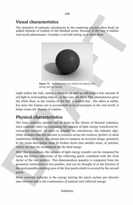
DRAF

T

246

Radiosity

Visual characteristicsThe inclusion of radiosity calculations in the rendering process often lends anadded element of realism to the finished scene, because of the way it mimicsreal-world phenomena. Consider a red ball sitting on a white floor.

Figure 75 Demonstration of a hybrid of radiosity ren-dering and ray tracing

Light strikes the ball, casting a shadow, as well as reflecting a tiny amount ofred light to surrounding objects - in this case, the floor. This phenomenon givesthe white floor, in the vicinity of the ball, a reddish hue. The effect is subtle,but since the human eye is accustomed to its counterpart in the real world, ithelps create the illusion of realism.

Physical characteristicsThe basic radiosity method has its basis in the theory of thermal radiation,since radiosity relies on computing the amount of light energy transferred be-tween two surfaces. In order to simplify the calculations, the radiosity algo-rithm assumes that this amount is constant across the surfaces (perfect or idealLambertian surfaces); this means that to compute an accurate image, geometryin the scene description must be broken down into smaller areas, or patches,which can then be recombined for the final image.

After this breakdown, the amount of light energy transfer can be computed byusing the known reflectivity of the reflecting patch, combined with the formfactor of the two patches. This dimensionless quantity is computed from thegeometric orientation of two patches, and can be thought of as the fraction ofthe total possible emitting area of the first patch which is covered by the secondpatch.

More correctly radiosity is the energy leaving the patch surface per discretetime interval and is the combination of emitted and reflected energy:

DRAF

T

247

Radiosity

BidAi = EidAi +Ri∫j BjFjidAj

Where:

• Bi is the radiosity of patch i.• Ei is emitted energy.• Ri is the reflectivity of the patch, giving reflected energy by multiplying by

the incident energy (the energy which arrives from other patches).• All j (j 6= i) in the rendered environment are integrated for BjFjidAj, to

determine the energy leaving each patch j that arrives at patch i.• Fji is a constant form factor for the geometric relation between patch i and

each patch j.

The reciprocity:

FijAi = FjiAj

gives:

Bi = Ei +Ri∫j BjFij

For ease of use the integral is replaced and constant radiosity is assumed overthe patch, creating the simpler:

Bi = Ei +Ri∑n

j=1BjFji

This equation can then be applied to each patch. The equation is monochro-matic, so color radiosity rendering requires calculation for each of the requiredcolors.

The constant Fji can be calculated in a number of ways. Early methods useda hemicube (an imaginary cube centered upon the first surface to which thesecond surface was projected, devised by Cohen and Greenberg in 1985) toapproximate the form factor, which also solved the intervening patch problem.This is quite computationally expensive, because ideally form factors must bederived for every possible pair of patches, leading to a quadratic increase incomputation with added geometry.

LimitationsAs radiosity only deals with the global radiance transfer between objects,position-dependent effects such as reflection (including specular lighting) and

DRAF

T

248

Ray casting

refraction cannot be simulated directly with this method. However, some sys-tems use hybrid approaches, making use of radiosity for illumination and raytracing (or some other technique) for position-dependent effects.

External links

• Radiosity, by Hugo Elias270 (also provides a general overview of lightingalgorithms, along with programming examples)

• Radiosity, by Allen Martin271 (a slightly more mathematical explanation ofradiosity)

Source: http://en.wikipedia.org/wiki/Radiosity

Principal Authors: Wapcaplet, Osmaker, Sallymander, Snorbaard, Uriyan, Mintleaf

Ray casting

Ray casting is not a synonym for ray tracing, but can be thought of as anabridged, and significantly faster, version of the ray tracing algorithm. Both areimage order algorithms used in computer graphics to render three dimensionalscenes to two dimensional screens by following rays of light from the eye ofthe observer to a light source. Ray casting does not compute the new tangentsa ray of light might take after intersecting a surface on its way from the eyeto the source of light. This eliminates the possibility of accurately renderingreflections, refractions, or the natural fall off of shadows – however all of theseelements can be faked to a degree, by creative use of texture maps or othermethods. The high speed of calculation made ray casting a handy method forthe rendering in early real-time 3D video games.

In nature, a light source emits a ray of light which travels, eventually, to asurface that interrupts its progress. One can think of this "ray" as a stream ofphotons travelling along the same path. At this point, any combination of threethings might happen with this light ray: absorption, reflection, and refraction.The surface may reflect all or part of the light ray, in one or more directions.It might also absorb part of the light ray, resulting in a loss of intensity of the

http://freespace.virgin.net/hugo.elias/radiosity/radiosity.htm270

http://web.cs.wpi.edu/~matt/courses/cs563/talks/radiosity.html271

DRAF

T

249

Ray casting

reflected and/or refracted light. If the surface has any transparent or translu-cent properties, it refracts a portion of the light beam into itself in a differentdirection while absorbing some (or all) of the spectrum (and possibly alteringthe color). Between absorption, reflection, and refraction, all of the incominglight must be accounted for, and no more. A surface cannot, for instance, re-flect 66% of an incoming light ray, and refract 50%, since the two would addup to be 116%. From here, the reflected and/or refracted rays may strike othersurfaces, where their absorptive, refractive, and reflective properties are againcalculated based on the incoming rays. Some of these rays travel in such away that they hit our eye, causing us to see the scene and so contribute to thefinal rendered image. Attempting to simulate this real-world process of tracinglight rays using a computer can be considered extremely wasteful, as only aminuscule fraction of the rays in a scene would actually reach the eye.

The first ray casting (versus ray tracing) algorithm used for rendering waspresented by A. Appel in 1968. The idea behind ray casting is to shoot raysfrom the eye, one per pixel, and find the closest object blocking the path ofthat ray - think of an image as a screen-door, with each square in the screenbeing a pixel. This is then the object the eye normally sees through that pixel.Using the material properties and the effect of the lights in the scene, thisalgorithm can determine the shading of this object. The simplifying assumptionis made that if a surface faces a light, the light will reach that surface and not beblocked or in shadow. The shading of the surface is computed using traditional3D computer graphics shading models. One important advantage ray castingoffered over older scanline algorithms is its ability to easily deal with non-planar surfaces and solids, such as cones and spheres. If a mathematical surfacecan be intersected by a ray, it can be rendered using ray casting. Elaborateobjects can be created by using solid modelling techniques and easily rendered.

Ray casting for producing computer graphics was first used by scientists atMathematical Applications Group, Inc., (MAGI) of Elmsford, New York, NewYork. In 1966 the company was created to perform radiation exposure calcula-tions for the Department of Defense. MAGI’s software calculated not only howthe gamma rays bounced off of surfaces (ray casting for radiation had beendone since the 1940s), but also how they penetrated and refracted within.These studies helped the government to determine certain military applica-tions ; constructing military vehicles that would protect troops from radiation,designing re-entry vehicles for space exploration. Under the direction of Dr.Philip Mittelman, the scientists developed a method of generating images us-ing the same basic software. In 1972 MAGI became a commercial animationstudio. This studio used ray casting to generate 3-D computer animation for

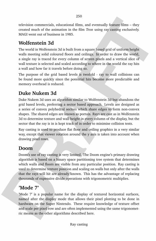
DRAF

T

250

Ray casting

television commercials, educational films, and eventually feature films – theycreated much of the animation in the film Tron using ray casting exclusively.MAGI went out of business in 1985.

Wolfenstein 3dThe world in Wolfenstein 3d is built from a square based grid of uniform heightwalls meeting solid coloured floors and ceilings. In order to draw the world,a single ray is traced for every column of screen pixels and a vertical slice ofwall texture is selected and scaled according to where in the world the ray hitsa wall and how far it travels before doing so.

The purpose of the grid based levels is twofold - ray to wall collisions canbe found more quickly since the potential hits become more predictable andmemory overhead is reduced.

Duke Nukem 3dDuke Nukem 3d uses an algorithm similar to Wolfenstein 3d but abandons thegrid based levels, preferring a sector based approach. Levels are designed asa series of convex polyhedral sectors which share edges to form non-convexshapes. The shared edges are known as portals. Rays are cast as in Wolfenstein3d to determine texture and wall height in every column of the display, but thesector that the ray is in is kept track of in order to minimise collision tests.

Ray casting is used to produce flat floor and ceiling graphics in a very similarway, except that viewer rotation around the y axis is taken into account whendrawing pixel rows.

DoomDoom’s use of ray casting is very limited. The Doom engine’s primary drawingalgorithm is based on a binary space partitioning tree system that determineswhich walls and floors are visible from any particular position. Ray casting isused to determine texture position and scaling on walls but only after the wallsthat the rays will hit are already known. This has the advantage of replacingthousands of expensive divide operations with trigonometric multiplies.

’Mode 7’’Mode 7’ is a popular name for the display of textured horizontal surfaces,named after the display mode that allows their pixel plotting to be done inhardware on the Super Nintendo. These require knowledge of texture offsetand scale per pixel row and are often implemented using the same trigonomet-ric means as the other algorithms described here.

DRAF

T

251

Ray tracing

References and External links

• Wolfenstein style Ray-Casting Tutorial by F. Permadi272

• Programming a Raycasting Engine Tutorial(QBasic) by Joe King273

• James D. Foley : Computer Graphics: Principles and Practice, Addison-Wesley 1995, ISBN 02-018-4840-6

Source: http://en.wikipedia.org/wiki/Ray_casting

Principal Authors: Mikhajist, RzR, DaveGorman, Pinbucket, Iamhove, Silsor, Reedbeta

Ray tracing

Figure 76 A ray-traced scene

http://www.permadi.com/tutorial/raycast/272

http://killfest.sytes.net/deltacode/tutorials1.shtml273

DRAF

T

252

Ray tracing

Ray tracing is a general technique from geometrical optics of modelling thepath taken by light by following rays of light as they interact with opticalsurfaces. It is used in the design of optical systems, such as camera lenses,microscopes, telescopes and binoculars. The term is also applied to mean aspecific rendering algorithmic approach in →3D computer graphics, wheremathematically-modelled visualisations of programmed scenes are producedusing a technique which follows rays from the eyepoint outward, rather thanoriginating at the light sources. It produces results similar to ray casting andscanline rendering, but facilitates more advanced optical effects, such as ac-curate simulations of reflection and refraction, and is still efficient enough tofrequently be of practical use when such high quality output is sought.

Broad description of ray tracing computer algo-rithm

Figure 77 Three spheres, that reflect off the floor and each other

Ray tracing describes a more realistic method than either ray casting or scan-line rendering, for producing visual images constructed in →3D computergraphics environments. It works by tracing in reverse, a path that could havebeen taken by a ray of light which would intersect the imaginary camera lens.As the scene is traversed by following in reverse the path of a very large number

DRAF

T

253

Ray tracing

of such rays, visual information on the appearance of the scene as viewed fromthe point of view of the camera, and in lighting conditions specified to the soft-ware, is built up. The ray’s reflection, refraction, or absorption are calculatedwhen it intersects objects and media in the scene.

Scenes in raytracing are described mathematically, usually by a programmer, orby a visual artist using intermediary tools, but they may also incorporate datafrom images and models captured by various technological means, for instancedigital photography.

Following rays in reverse is many orders of magnitude more efficient at build-ing up the visual information than would be a genuine simulation of light inter-actions, since the overwhelming majority of light rays from a given light sourcedo not wind up providing significant light to the viewers eye, but instead maybounce around until they diminish to almost nothing, or bounce off to infinity.A computer simulation starting with the rays emitted by the light source andlooking for ones which wind up intersecting the viewpoint is not practicallyfeasible to execute and obtain accurate imagery.

The obvious shortcut is to pre-suppose that the ray ends up at the viewpoint,then trace backwards. After a stipulated number of maximum reflections hasoccurred, the light intensity of the point of last intersection is estimated using anumber of algorithms, which may include the classic rendering algorithm, andmay perhaps incorporate other techniques such as radiosity.

Detailed description of ray tracing computer algo-rithm and its genesis

What happens in natureIn nature, a light source emits a ray of light which travels, eventually, to asurface that interrupts its progress. One can think of this "ray" as a stream ofphotons travelling along the same path. In a perfect vacuum this ray will be astraight line. In reality, any combination of three things might happen with thislight ray: absorption, reflection, and refraction. A surface may reflect all or partof the light ray, in one or more directions. It might also absorb part of the lightray, resulting in a loss of intensity of the reflected and/or refracted light. If thesurface has any transparent or translucent properties, it refracts a portion of thelight beam into itself in a different direction while absorbing some (or all) ofthe spectrum (and possibly altering the color). Between absorption, reflection,and refraction, all of the incoming light must be accounted for, and no more.A surface cannot, for instance, reflect 66% of an incoming light ray, and refract

DRAF

T

254

Ray tracing

50%, since the two would add up to be 116%. From here, the reflected and/orrefracted rays may strike other surfaces, where their absorptive, refractive, andreflective properties are again calculated based on the incoming rays. Someof these rays travel in such a way that they hit our eye, causing us to see thescene and so contribute to the final rendered image. Attempting to simulatethis real-world process of tracing light rays using a computer can be consideredextremely wasteful, as only a minuscule fraction of the rays in a scene wouldactually reach the eye.

Ray casting algorithmThe first ray casting (versus ray tracing) algorithm used for rendering waspresented by Arthur Appel in 1968. The idea behind ray casting is to shootrays from the eye, one per pixel, and find the closest object blocking the pathof that ray - think of an image as a screen-door, with each square in the screenbeing a pixel. This is then the object the eye normally sees through that pixel.Using the material properties and the effect of the lights in the scene, thisalgorithm can determine the shading of this object. The simplifying assumptionis made that if a surface faces a light, the light will reach that surface and not beblocked or in shadow. The shading of the surface is computed using traditional3D computer graphics shading models. One important advantage ray castingoffered over older scanline algorithms is its ability to easily deal with non-planar surfaces and solids, such as cones and spheres. If a mathematical surfacecan be intersected by a ray, it can be rendered using ray casting. Elaborateobjects can be created by using solid modelling techniques and easily rendered.

Ray casting for producing computer graphics was first used by scientists atMathematical Applications Group, Inc., (MAGI) of Elmsford, New York, NewYork. In 1966, the company was created to perform radiation exposure calcula-tions for the Department of Defense. MAGI’s software calculated not only howthe gamma rays bounced off of surfaces (ray casting for radiation had beendone since the 1940s), but also how they penetrated and refracted within.These studies helped the government to determine certain military applica-tions ; constructing military vehicles that would protect troops from radiation,designing re-entry vehicles for space exploration. Under the direction of Dr.Philip Mittelman, the scientists developed a method of generating images us-ing the same basic software. In 1972, MAGI became a commercial animationstudio. This studio used ray casting to generate 3-D computer animation fortelevision commercials, educational films, and eventually feature films – theycreated much of the animation in the film Tron using ray casting exclusively.MAGI went out of business in 1985.

DRAF

T

255

Ray tracing

Ray tracing algorithmThe next important research breakthrough came from Turner Whitted in 1979.Previous algorithms cast rays from the eye into the scene, but the rays weretraced no further. Whitted continued the process. When a ray hits a surface,it could generate up to three new types of rays: reflection, refraction, andshadow. A reflected ray continues on in the mirror-reflection direction from ashiny surface. It is then intersected with objects in the scene; the closest objectit intersects is what will be seen in the reflection. Refraction rays travelingthrough transparent material work similarly, with the addition that a refractiveray could be entering or exiting a material. To further avoid tracing all raysin a scene, a shadow ray is used to test if a surface is visible to a light. A rayhits a surface at some point. If the surface at this point faces a light, a ray (tothe computer, a line segment) is traced between this intersection point and thelight. If any opaque object is found in between the surface and the light, thesurface is in shadow and so the light does not contribute to its shade. This newlayer of ray calculation added more realism to ray traced images.

Advantages of ray tracingRay tracing’s popularity stems from its basis in a realistic simulation of light-ing over other rendering methods (such as scanline rendering or ray casting).Effects such as reflections and shadows, which are difficult to simulate usingother algorithms, are a natural result of the ray tracing algorithm. Relativelysimple to implement yet yielding impressive visual results, ray tracing oftenrepresents a first foray into graphics programming.

Disadvantages of ray tracingA serious disadvantage of ray tracing is performance. Scanline algorithms andother algorithms use data coherence to share computations between pixels,while ray tracing normally starts the process anew, treating each eye ray sepa-rately. However, this separation offers other advantages, such as the ability toshoot more rays as needed to perform anti-aliasing and improve image qual-ity where needed. Although it does handle interreflection and optical effectssuch as refraction accurately, traditional Ray Tracing is also not necessarilyphotorealistic. True photorealism occurs when the rendering equation is close-ly approximated or fully implemented. Implementing the rendering equationgives true photorealism. As the equation describes every physical effect of lightflow. However, this is usually infeasable given the computing resources re-quired. The realism of all rendering methods, then, must be evaluated as an

DRAF

T

256

Ray tracing

approximation to the equation, and in the case of Ray Tracing, it is not neces-sarily the most realistic. Other methods, including photon mapping, are basedupon raytracing for certain parts of the algorithm, yet give far better results.

Reversed direction of traversal of scene by the raysThe process of shooting rays from the eye to the light source to render an im-age is sometimes referred to as backwards ray tracing, since it is the oppositedirection photons actually travel. However, there is confusion with this termi-nology. Early ray tracing was always done from the eye, and early researcherssuch as James Arvo used the term backwards ray tracing to refer to shootingrays from the lights and gathering the results. As such, it is clearer to distin-guish eye-based versus light-based ray tracing. Research over the past decadeshas explored combinations of computations done using both of these direc-tions, as well as schemes to generate more or fewer rays in different directionsfrom an intersected surface. For example, radiosity algorithms typically workby computing how photons emitted from lights affect surfaces and storing theseresults. This data can then be used by a standard recursive ray tracer to cre-ate a more realistic and physically correct image of a scene. In the context ofglobal illumination algorithms, such as photon mapping and →Metropolis lighttransport, ray tracing is simply one of the tools used to compute light transferbetween surfaces.

Algorithm: classical recursive ray tracing

For each pixel in image Create ray from eyepoint passing through this pixel

Initialize NearestT to INFINITY and NearestObject to NULL

For every object in scene If ray intersects this object

If t of intersection is less than NearestT Set NearestT to t of the intersection

Set NearestObject to this object

If NearestObject is NULL Fill this pixel with background color

Else Shoot a ray to each light source to check if in shadow

DRAF

T

257

Ray tracing

If surface is reflective, generate reflection ray: recurse

If surface is transparent, generate refraction ray: re-

curse

Use NearestObject and NearestT to compute shading function

Fill this pixel with color result of shading function

Ray tracing in real timeThere has been some effort for implementing ray tracing in real time speedsfor interactive 3D graphics applications such as computer and video games.

The→OpenRT project includes a highly-optimized software core for ray tracingalong with an →OpenGL-like API in order to offer an alternative to the currentrasterization based approach for interactive 3D graphics.

→Ray tracing hardware, such as the experimental Ray Processing Unit devel-oped at the Saarland University, has been designed to accelerate some of thecomputationally intensive operations of ray tracing.

Some real-time software 3D engines based on ray tracing have been developedby hobbyist demo programmers since the late 1990’s. The ray tracers usedin demos, however, often use inaccurate approximations and even cheating inorder to attain reasonably high frame rates. 274

In optical designRay tracing in computer graphics derives its name and principles from a mucholder technique used for lens design since the 1900s. Geometric ray tracing isused to describe the propagation of light rays through a lens system or opticalinstrument, allowing the image-forming properties of the system to be mod-eled. This is used to optimize the design of the instrument (e.g. to minimizeeffects such as chromatic and other aberrations) before it is built. Ray tracing isalso used to calculate optical path differences through optical systems, whichare used to calculate optical wavefronts, which in turn are used to calculatesystem diffraction effects such as point spread function, MTF, and Strehl ratio.It is not only used for designing lenses, as for photography, but can also be usedfor longer wavelength applications such as designing microwave or even radiosystems, and for shorter wavelengths, such as ultraviolet and X-ray optics.

http://www.acm.org/tog/resources/RTNews/demos/overview.htm274

DRAF

T

258

Ray tracing

The principles of ray tracing for computer graphics and optical design are sim-ilar, but the technique in optical design usually uses much more rigorous andphysically correct models of how light behaves. In particular, optical effectssuch as dispersion, diffraction and the behaviour of optical coatings are impor-tant in lens design, but are less so in computer graphics.

Before the advent of the computer, ray tracing calculations were performed byhand using trigonometry and logarithmic tables. The optical formulas of manyclassic photographic lenses were optimized by rooms full of people, each ofwhom handled a small part of the large calculation. Now they are worked outin optical design software such as OSLO or TracePro from Lambda Research,Code-V or Zemax. A simple version of ray tracing known as ray transfer matrixanalysis is often used in the design of optical resonators used in lasers.

ExampleAs a demonstration of the principles involved in raytracing, let us considerhow one would find the intersection between a ray and a sphere. The generalequation of a sphere, where I is a point on the surface of the sphere, C is itscentre and r is its radius, is |I − C|2 = r2. Equally, if a line is defined by itsstarting point S (consider this the starting point of the ray) and its direction d(consider this the direction of that particular ray), each point on the line maybe described by the expression

S + td ,

where t is a constant defining the distance along the line from the startingpoint (hence, for simplicity’s sake, d is generally a unit vector). Now, in thescene we know S, d, C, and r. Hence we need to find t as we substitute in forI:

|S + td− C|2 = r2 .

Let V ≡ S− C for simplicity, then

|V + td|2 = r2

V 2 + t2d2 + 2V · dt = r2

d2t2 + 2V · dt+ V 2 − r2 = 0 .

Now this quadratic equation has solutions

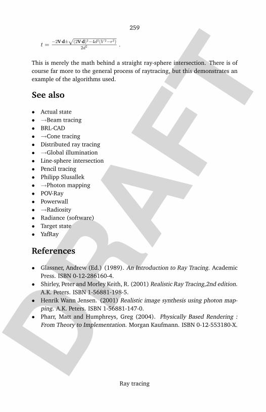
DRAF

T

259

Ray tracing

t = −2V·d±√

(2V·d)2−4d2(V 2−r2)2d2 .

This is merely the math behind a straight ray-sphere intersection. There is ofcourse far more to the general process of raytracing, but this demonstrates anexample of the algorithms used.

See also

• Actual state• →Beam tracing• BRL-CAD• →Cone tracing• Distributed ray tracing• →Global illumination• Line-sphere intersection• Pencil tracing• Philipp Slusallek• →Photon mapping• POV-Ray• Powerwall• →Radiosity• Radiance (software)• Target state• YafRay

References

• Glassner, Andrew (Ed.) (1989). An Introduction to Ray Tracing. AcademicPress. ISBN 0-12-286160-4.

• Shirley, Peter and Morley Keith, R. (2001) Realistic Ray Tracing,2nd edition.A.K. Peters. ISBN 1-56881-198-5.

• Henrik Wann Jensen. (2001) Realistic image synthesis using photon map-ping. A.K. Peters. ISBN 1-56881-147-0.

• Pharr, Matt and Humphreys, Greg (2004). Physically Based Rendering :From Theory to Implementation. Morgan Kaufmann. ISBN 0-12-553180-X.

DRAF

T

260

Ray tracing

External links

• The Ray Tracing News275 - short research articles and new links to resources• Games using realtime raytracing276

• A series of raytracing tutorials for the implementation of an efficient ray-tracer using C++277

• Mini ray tracers written equivalently in various languages278

Raytracing software

• POV-Ray279

• PBRT280 - a Physically Based Raytracer• Tachyon281

• Rayshade282

• OpenRT283 - realtime raytracing library• Raster3D284

• RealStorm Engine285 - a realtime raytracing engine• BRL-CAD286

• More ray tracing source code links287

• Zemax288

• Radiance289

• Yafray290

• OSLO291 - Lens design and optimization software; OSLO-EDU is a freedownload

• TracePro292 - Straylight and illumination software with a CAD-like interface

http://www.raytracingnews.org/275

http://graphics.cs.uni-sb.de/RTGames/276

http://www.devmaster.net/articles/raytracing_series/part1.php277

http://www.ffconsultancy.com/free/ray_tracer/languages.html278

http://www.povray.org/279

http://www.pbrt.org280

http://jedi.ks.uiuc.edu/~johns/raytracer281

http://graphics.stanford.edu/~cek/rayshade282

http://www.openrt.de/283

http://www.bmsc.washington.edu/raster3d/raster3d.html284

http://www.realstorm.com285

http://brlcad.org/286

http://www.acm.org/tog/Software.html#ray287

http://www.zemax.com/288

http://radsite.lbl.gov/radiance/289

http://www.yafray.org290

http://www.lambdares.com/products/oslo/291

http://www.lambdares.com/products/tracepro/292

DRAF

T

261

Ray tracing hardware

Source: http://en.wikipedia.org/wiki/Ray_tracing

Principal Authors: Pinbucket, DrBob, Srleffler, Jawed, Osmaker, Carrionluggage, ToastieIL, Steverti-

go, Viznut, Ed g2s

Ray tracing hardware

Ray tracing hardware is a special purpose computer hardware design for ac-celerating real-time ray tracing.

Ray Tracing vs. RasterizationThe problem of rendering 3D graphics can be conceptually presented as findingall intersections between a set of "primitives" (typically triangles or polygons)and a set of "rays" (typically one or more per pixel).

Typical graphic acceleration boards, so called GPUs use rasterization algorithm.In this approach, in each step, the GPU finds all intersections of a single prim-itive and all rays of the screen. Well known brands such as intel, NVIDIA andATI have developed very efficient algorithms to do so.

The ray tracing algorithm solves the rendering problem in a different way. Ineach step, it finds all intersections of a single ray with all primitives of thescene. The ray tracing algorithm has been around for some decades, but onlyrecent research from the Universities of Saarland and Utah, as well as inTraceGmbH have led to the first interactive ray tracing application that is able tocompute this algorithm at several frames per second.

Both approaches have different benefits and drawbacks. Rasterization can beperformed in a stream-like manner, one triangle at the time, and access tocomplete scene is not needed. The drawback of rasterization is that non-localeffects, like reflections, refraction, shadows and realistic lighting, are very dif-ficult to compute.

The ray tracing algorithm can also be parallelized very well, if one considerseach ray separately, however its memory bandwidth is crucial as various partsof the scene need to be accessed. But it can easily compute various kindsof physically correct effects, providing much more realistic impression thanrasterization.

An additional advantage is logarithmic complexity of ray tracing in number ofscene objects and possibility of using more complex primitives without their

DRAF

T

262

Reflection mapping

prior triangulation. The biggest drawback for real time ray tracing is the needfor quite costly recomputations of spatial index structures in case of highlydynamic scenes. Some problems remain to be solved, such as ray tracing oflines and text.

ImplementationsToday there are two existing implementations of ray tracing hardware:

• There is the ART VPS company, situated in the UK, that sells ray tracinghardware for offline rendering.

• There is the Saarland University, striving to develop a real-time ray tracingchip, so far they have published two designs: SaarCOR and the RPU.

See also

• →OpenRT Only available real time ray tracing software

External links

• ART VPS293

Source: http://en.wikipedia.org/wiki/Ray_tracing_hardware

Reflection mapping

In Computer Graphics, reflection mapping is an efficient method of simulatinga complex mirroring surface by means of a precomputed texture image. Thetexture is used to store the image of the environment surrounding the renderedobject. There are several ways of storing the surrounding enviromnent; themost common ones are the Standard Environment Mapping in which a singletexture contains the image of the surrounding as reflected on a mirror ball, orthe Cubic Environment Mapping in which the envirornment is unfolded ontothe six faces of a cube and stored therefore as six square textures.

This kind of approach is more efficient than the classical ray tracing approachof computing the exact reflection by shooting a ray and following its optically

http://www.art-render.com/293

DRAF

T

263

Reflection mapping

Figure 78 An example of reflection mapping. Observe the crudeness of the output.

exact path, but it should be noted that these are (sometimes crude) approxima-tion of the real reflection. A typical drawback of this technique is the absenceof self reflections: you cannot see any part of the reflected object inside thereflection itself.

Types of Reflection Mapping

Standard Environment MappingStandard environment mapping, more commonly known as spherical envi-ronment mapping, involves the use of a textured sphere infinitely far awayfrom the object that reflects it. By creating a spherical texture using a fisheyelens or via prerendering or with a light probe, this texture is mapped to a hol-low sphere, and the texel colors are determined by calculating the light vectorsfrom the points on the object to the texels in the environment map. This tech-nique is similar to raytracing, but incurs less of a performance hit because allof the colors of the points to be referenced are known beforehand by the GPU,so all it has to do is to calculate the angles of incidence and reflection.

There are a few glaring limitations to spherical mapping. For one thing, dueto the nature of the texture used for the map, there is an abrupt point of sin-gularity on the backside of objects using spherical mapping. Cube mapping

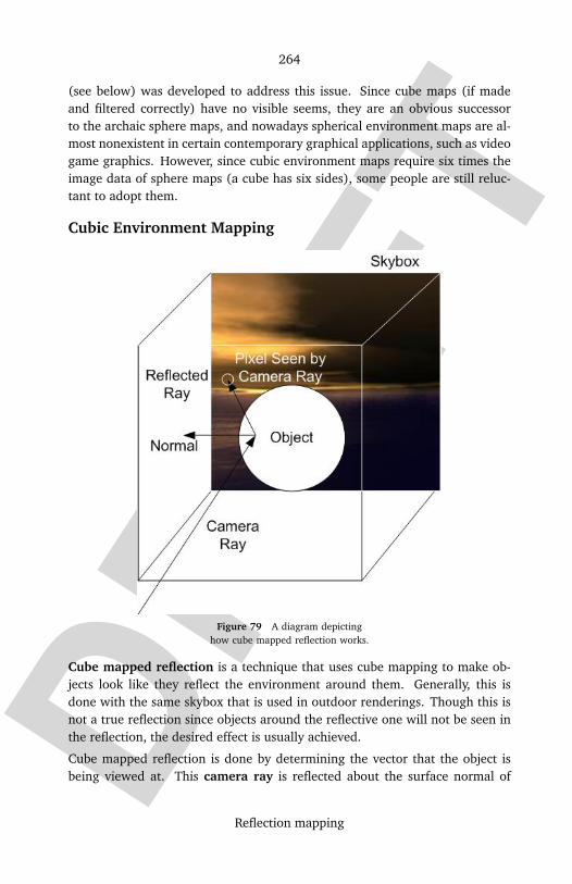
DRAF

T

264

Reflection mapping

(see below) was developed to address this issue. Since cube maps (if madeand filtered correctly) have no visible seems, they are an obvious successorto the archaic sphere maps, and nowadays spherical environment maps are al-most nonexistent in certain contemporary graphical applications, such as videogame graphics. However, since cubic environment maps require six times theimage data of sphere maps (a cube has six sides), some people are still reluc-tant to adopt them.

Cubic Environment Mapping

Figure 79 A diagram depictinghow cube mapped reflection works.

Cube mapped reflection is a technique that uses cube mapping to make ob-jects look like they reflect the environment around them. Generally, this isdone with the same skybox that is used in outdoor renderings. Though this isnot a true reflection since objects around the reflective one will not be seen inthe reflection, the desired effect is usually achieved.

Cube mapped reflection is done by determining the vector that the object isbeing viewed at. This camera ray is reflected about the surface normal of

DRAF

T

265

Reflection mapping

where the camera vector intersects the object. This results in the reflected raywhich is then passed to the cube map to get the texel which the camera thensees as if it is on the surface of the object. This creates the effect that the objectis reflective.

Application in Real-Time 3D Graphics

Standard Environment Mapping

Cubic Environment Mapping

Figure 80 Example of a three-dimensionalmodel using cube mapped reflection

Cube mapped reflection, when used correctly, may be the fastest method ofrendering a reflective surface. To increase the speed of rendering, each vertexcalculates the position of the reflected ray. Then, the position is interpolatedacross polygons to which the vertex is attached. This eliminates the need forrecalculating every pixel’s reflection.

DRAF

T

266

Rendering (computer graphics)

See Also

• The Story of Reflection mapping294 cured by Paul Debevec• Skybox (video games)• →Cube mapping

Source: http://en.wikipedia.org/wiki/Reflection_mapping

Principal Authors: ALoopingIcon, Gaius Cornelius, Abdull, Srleffler, Freeformer


Rendering is the process of generating an image from a model, by means ofa software program. The model is a description of three dimensional objectsin a strictly defined language or data structure. It would contain geometry,viewpoint, texture and lighting information. The image is a digital image orraster graphics image. The term may be by analogy with an "artist’s rendering"of a scene. ’Rendering’ is also used to describe the process of calculating effectsin a video editing file to produce final video output.

It is one of the major sub-topics of →3D computer graphics, and in practicealways connected to the others. In the ’graphics pipeline’ it’s the last major step,giving the final appearance to the models and animation. With the increasingsophistication of computer graphics since the 1970s onward, it has become amore distinct subject.

It has uses in: computer and video games, simulators, movies or TV special ef-fects, and design visualisation, each employing a different balance of featuresand techniques. As a product, a wide variety of renderers are available. someare integrated into larger modelling and animation packages, some are stand-alone, some are free open-source projects. On the inside, a renderer is a care-fully engineered program, based on a selective mixture of disciplines relatedto: light physics, visual perception, mathematics, and software development.

In the case of 3D graphics, rendering may be done slowly, as in pre-rendering,or in real time. Pre-rendering is a computationally intensive process that istypically used for movie creation, while real-time rendering is often done for

http://www.debevec.org/ReflectionMapping/294

DRAF

T

267


3D video games which rely on the use of graphics cards with 3D hardwareaccelerators.

UsageWhen the pre-image (a wireframe sketch usually) is complete, rendering isused, which adds in bitmap textures or procedural textures, lights, bump map-ping, and relative position to other objects. The result is a completed imagethe consumer or intended viewer sees.

For movie animations, several images (frames) must be rendered, and stitchedtogether in a program capable of making an animation of this sort. Most 3Dimage editing programs can do this.

FeaturesA rendered image can be understood in terms of a number of visible features.Rendering research and development has been largely motivated by findingways to simulate these efficiently. Some relate directly to particular algorithmsand techniques, while others are produced together.

• shading — how the color and brightness of a surface varies with lighting• texture-mapping — a method of applying detail to surfaces• bump-mapping — a method of simulating small-scale bumpiness on sur-

faces• fogging/participating medium — how light dims when passing through

non-clear atmosphere or air• shadows — the effect of obstructing light• soft shadows — varying darkness caused by partially obscured light

sources• reflection — mirror-like or highly glossy reflection• transparency — sharp transmission of light through solid objects• translucency — highly scattered transmission of light through solid objects• refraction — bending of light associated with transparency• indirect illumination — surfaces illuminated by light reflected off other

surfaces, rather than directly from a light source• caustics (a form of indirect illumination) — reflection of light off a shiny

object, or focusing of light through a transparent object, to produce brighthighlights on another object

• depth of field — objects appear blurry or out of focus when too far in frontof or behind the object in focus

• motion blur — objects appear blurry due to high-speed motion, or themotion of the camera

DRAF

T

268


• photorealistic morphing — photoshopping 3D renderings to appear morelife-like

• non-photorealistic rendering — rendering of scenes in an artistic style,intended to look like a painting or drawing

TechniquesMany rendering algorithms have been researched, and software used for ren-dering may employ a number of different techniques to obtain a final image.

Tracing every ray of light in a scene would be impractical and would takegigantic amounts of time. Even tracing a portion large enough to produce animage takes an inordinate amount of time if the sampling is not intelligentlyrestricted.

Therefore, four loose families of more-efficient light transport modelling tech-niques have emerged: rasterisation, including scanline rendering, considersthe objects in the scene and projects them to form an image, with no facili-ty for generating a point-of-view perspective effect; ray casting considers thescene as observed from a specific point-of-view, calculating the observed imagebased only on geometry and very basic optical laws of reflection intensity, andperhaps using Monte Carlo techniques to reduce artifacts; radiosity uses fi-nite element mathematics to simulate diffuse spreading of light from surfaces;and ray tracing is similar to ray casting, but employs more advanced opticalsimulation, and usually uses Monte Carlo techniques, to obtain more realisticresults, at a speed which is often orders of magnitude slower.

Most advanced software combines two or more of the techniques to obtaingood-enough results at reasonable cost.

Scanline rendering and rasterisationA high-level representation of an image necessarily contains elements in a dif-ferent domain from pixels. These elements are referred to as primitives. In aschematic drawing, for instance, line segments and curves might be primitives.In a graphical user interface, windows and buttons might be the primitives. In3D rendering, triangles and polygons in space might be primitives.

If a pixel-by-pixel approach to rendering is impractical or too slow for sometask, then a primitive-by-primitive approach to rendering may prove useful.Here, one loops through each of the primitives, determines which pixels in theimage it affects, and modifies those pixels accordingly. This is called rasteriza-tion, and is the rendering method used by all current graphics cards.

DRAF

T

269


Rasterization is frequently faster than pixel-by-pixel rendering. First, large ar-eas of the image may be empty of primitives; rasterization will ignore theseareas, but pixel-by-pixel rendering must pass through them. Second, rasteri-zation can improve cache coherency and reduce redundant work by taking ad-vantage of the fact that the pixels occupied by a single primitive tend to be con-tiguous in the image. For these reasons, rasterization is usually the approach ofchoice when interactive rendering is required; however, the pixel-by-pixel ap-proach can often produce higher-quality images and is more versatile becauseit does not depend on as many assumptions about the image as rasterization.

Rasterization exists in two main forms, not only when an entire face (primitive)is rendered but when the vertices of a face are all rendered and then the pixelson the face which lie between the vertices rendered using simple blending ofeach vertex colour to the next, this version of rasterization has overtaken theold method as it allows the graphics to flow without complicated textures (arasterized image when used face by face tends to have a very block like effectif not covered in complex textures, the faces aren’t smooth because there isno gradual smoothness from one pixel to the next,) this meens that you canutilise the graphics card’s more taxing shading functions and still achieve betterperformance because you have freed up space o the card because complextextures aren’t necessary. sometimes people will use one rasterization methodon some faces and the other method on others based on the angle at whichthat face meets other joined faces, this can increase speed and not take awaytoo much from the images overall effect.

Ray castingRay casting is primarily used for realtime simulations, such as those used in3D computer games and cartoon animations, where detail is not important, orwhere it is more efficient to manually fake the details in order to obtain betterperformance in the computational stage. This is usually the case when a largenumber of frames need to be animated. The results have a characteristic ’flat’appearance when no additional tricks are used, as if objects in the scene wereall painted with matt finish, or had been lightly sanded.

The geometry which has been modelled is parsed pixel by pixel, line by line,from the point of view outward, as if casting rays out from the point of view.Where an object is intersected, the colour value at the point may be evaluatedusing several methods. In the simplest, the colour value of the object at thepoint of intersection becomes the value of that pixel. The colour may be de-termined from a texture-map. A more sophisticated method is to modify thecolour value by an illumination factor, but without calculating the relationship

DRAF

T

270


to a simulated light source. To reduce artifacts, a number of rays in slightlydifferent directions may be averaged.

Rough simulations of optical properties may be additionally employed: com-monly, making a very simple calculation of the ray from the object to the pointof view. Another calculation is made of the angle of incidence of light raysfrom the light source(s). And from these and the specified intensities of thelight sources, the value of the pixel is calculated.

Or illumination plotted from a radiosity algorithm could be employed. Or acombination of these.

Radiosity→Radiosity is a method which attempts to simulate the way in which reflectedlight, instead of just reflecting to another surface, also illuminates the areaaround it. This produces more realistic shading and seems to better capturethe ’ambience’ of an indoor scene. A classic example used is of the way thatshadows ’hug’ the corners of rooms.

The optical basis of the simulation is that some diffused light from a given pointon a given surface is reflected in a large spectrum of directions and illuminatesthe area around it.

The simulation technique may vary in complexity. Many renderings have a veryrough estimate of radiosity, simply illuminating an entire scene very slightlywith a factor known as ambiance. However, when advanced radiosity estima-tion is coupled with a high quality ray tracing algorithim, images may exhibitconvincing realism, particularly for indoor scenes.

In advanced radiosity simulation, recursive, finite-element algorithms ’bounce’light back and forth between surfaces in the model, until some recursion limitis reached. The colouring of one surface in this way influences the colouringof a neighbouring surface, and vice versa. The resulting values of illuminationthroughout the model (sometimes including for empty spaces) are stored andused as additional inputs when performing calculations in a ray-casting or ray-tracing model.

Due to the iterative/recursive nature of the technique, complex objects areparticularly slow to emulate. Advanced radiosity calculations may be reservedfor calulating the ambiance of the room, from the light reflecting off walls, floorand celiing, without examining the contribution that complex objects make tothe radiosity – or complex objects may be replaced in the radiosity calculationwith simpler objects of similar size and texture.

DRAF

T

271


If there is little rearrangement of radiosity objects in the scene, the same radios-ity data may be reused for a number of frames, making radiosity an effectiveway to improve on the flatness of ray casting, without seriously impacting theoverall rendering time-per-frame.

Because of this, radiosity has become the leading real-time rendering method,and has been used to beginning-to-end create a large number of well-knownrecent feature-length animated 3D-cartoon films.

Ray tracingRay tracing is an extension of the same technique developed in scanline ren-dering and ray casting. Like those, it handles complicated objects well, and theobjects may be described mathematically. Unlike scanline and casting, ray trac-ing is almost always a Monte Carlo technique, that is one based on averaginga number of randomly generated samples from a model.

In this case, the samples are imaginary rays of light intersecting the viewpointfrom the objects in the scene. It is primarily beneficial where complex andaccurate rendering of shadows, refraction or reflection are issues.

In a final, production quality rendering of a ray traced work, multiple rays aregenerally shot for each pixel, and traced not just to the first object of intersec-tion, but rather, through a number of sequential ’bounces’, using the knownlaws of optics such as "angle of incidence equals angle of reflection" and moreadvanced laws that deal with refraction and surface roughness.

Once the ray either encounters a light source, or more probably once a set lim-iting number of bounces has been evaluated, then the surface illumination atthat final point is evaluated using techniques described above, and the changesalong the way through the various bounces evaluated to estimate a value ob-served at the point of view. This is all repeated for each sample, for each pixel.

In some cases, at each point of intersection, multiple rays may be spawned.

As a brute-force method, raytracing has been too slow to consider for realtime,and until recently too slow even to consider for short films of any degree ofquality, although it has been used for special effects sequences, and in advertis-ing, where a short portion of high quality (perhaps even photorealistic) footageis required.

However, efforts at optimising to reduce the number of calculations needed inportions of a work where detail is not high or does not depend on raytracingfeatures have led to a realistic possibility of wider use of ray tracing. There isnow some hardware accelerated ray tracing equipment, at least in prototype

DRAF

T

272


phase, and some game demos which show use of realtime software or hardwareray tracing.

Optimisation

Optimisations used by an artist when a scene is being devel-opedDue to the large number of calulations, a work in progress is usually onlyrendered in detail appropriate to the portion of the work being developed at agiven time, so in the initial stages of modelling, wireframe and ray casting maybe used, even where the target output is ray tracing with radiosity. It is alsocommon to render only parts of the scene at high detail, and to remove objectsthat are not important to what is currently being developed.

Common optimisations for real time renderingFor real-time, it is appropriate to simplify one or more common approxima-tions, and tune to the exact parameters of the scenery in question, which isalso tuned to the agreed parameters to get the most ’bang for buck’.

There are some lesser known approaches to rendering, such as spherical har-monics. These techniques are lesser known often due to slow speed, lack ofpractical use or simply because they are in early stages of development; maybesome will offer a new solution.

Sampling and filteringOne problem that any rendering system must deal with, no matter which ap-proach it takes, is the sampling problem. Essentially, the rendering processtries to depict a continuous function from image space to colors by using a fi-nite number of pixels. As a consequence of the Nyquist theorem, the scanningfrequency must be twice the dot rate, which is proportional to image resolu-tion. In simpler terms, this expresses the idea that an image cannot displaydetails smaller than one pixel.

If a naive rendering algorithm is used, high frequencies in the image functionwill cause ugly aliasing to be present in the final image. Aliasing typicallymanifests itself as jaggies, or jagged edges on objects where the pixel grid isvisible. In order to remove aliasing, all rendering algorithms (if they are toproduce good-looking images) must filter the image function to remove highfrequencies, a process called antialiasing.

DRAF

T

273


See also

• the painter’s algorithm• Scanline algorithms like Reyes• Z-buffer algorithms• →Global illumination• →Radiosity• →Ray tracing• →Volume rendering

Rendering for movies often takes place on a network of tightly connected com-puters known as a render farm.

The current state of the art in 3-D image description for movie creation isthe RenderMan scene description language designed at Pixar. (compare withsimpler 3D fileformats such as VRML or APIs such as →OpenGL and DirectXtailored for 3D hardware accelerators).

Movie type rendering software includes:

• RenderMan compliant renderers• Mental Ray• Brazil• Blender (may also be used for modeling)• LightWave (includes modelling module)

Academic coreThe implementation of a realistic renderer always has some basic element ofphysical simulation or emulation — some computation which resembles or ab-stracts a real physical process.

The term "physically-based " indicates the use of physical models and approxi-mations that are more general and widely accepted outside rendering. A par-ticular set of related techniques have gradually become established in the ren-dering community.

The basic concepts are moderately straightforward, but intractable to calcu-late; and a single elegant algorithm or approach has been elusive for moregeneral purpose renderers. In order to meet demands of robustness, accuracy,and practicality, an implementation will be a complex combination of differenttechniques.

Rendering research is concerned with both the adaptation of scientific modelsand their efficient application.

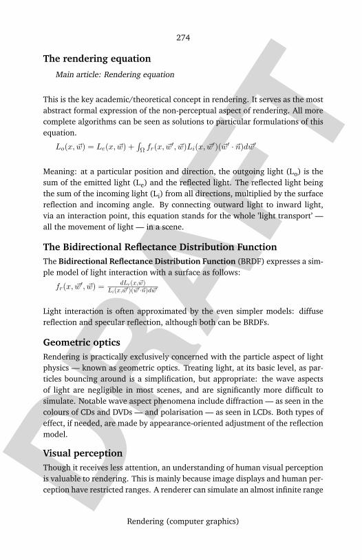
DRAF

T

274


The rendering equation

Main article: Rendering equation

This is the key academic/theoretical concept in rendering. It serves as the mostabstract formal expression of the non-perceptual aspect of rendering. All morecomplete algorithms can be seen as solutions to particular formulations of thisequation.

Lo(x, ~w) = Le(x, ~w) +∫Ω fr(x, ~w

′, ~w)Li(x, ~w′)(~w′ · ~n)d~w′

Meaning: at a particular position and direction, the outgoing light (Lo) is thesum of the emitted light (Le) and the reflected light. The reflected light beingthe sum of the incoming light (Li) from all directions, multiplied by the surfacereflection and incoming angle. By connecting outward light to inward light,via an interaction point, this equation stands for the whole ’light transport’ —all the movement of light — in a scene.

The Bidirectional Reflectance Distribution FunctionThe Bidirectional Reflectance Distribution Function (BRDF) expresses a sim-ple model of light interaction with a surface as follows:

fr(x, ~w′, ~w) = dLr(x,~w)Li(x,~w′)(~w′·~n)d~w′

Light interaction is often approximated by the even simpler models: diffusereflection and specular reflection, although both can be BRDFs.

Geometric opticsRendering is practically exclusively concerned with the particle aspect of lightphysics — known as geometric optics. Treating light, at its basic level, as par-ticles bouncing around is a simplification, but appropriate: the wave aspectsof light are negligible in most scenes, and are significantly more difficult tosimulate. Notable wave aspect phenomena include diffraction — as seen in thecolours of CDs and DVDs — and polarisation — as seen in LCDs. Both types ofeffect, if needed, are made by appearance-oriented adjustment of the reflectionmodel.

Visual perceptionThough it receives less attention, an understanding of human visual perceptionis valuable to rendering. This is mainly because image displays and human per-ception have restricted ranges. A renderer can simulate an almost infinite range

DRAF

T

275


of light brightness and color, but current displays — movie screen, computermonitor, etc. — cannot handle so much, and something must be discarded orcompressed. Human perception also has limits, and so doesn’t need to be givenlarge-range images to create realism. This can help solve the problem of fittingimages into displays, and, furthermore, suggest what short-cuts could be usedin the rendering simulation, since certain subtleties won’t be noticeable. Thisrelated subject is tone mapping.

Mathematics used in rendering includes: linear algebra, calculus, numericalmathematics, signal processing, monte carlo.

Chronology of important published ideas

• 1970 Scan-line algorithm (Bouknight, W. J. (1970). A procedure forgeneration of three-dimensional half-tone computer graphics presentations.Communications of the ACM)

• 1971 Gouraud shading (Gouraud, H. (1971). Computer display of curvedsurfaces. IEEE Transactions on Computers 20 (6), 623–629.)

• 1974 Texture mapping (Catmull, E. (1974). A subdivision algorithm forcomputer display of curved surfaces. PhD thesis, University of Utah.)

• 1974 Z-buffer (Catmull, E. (1974). A subdivision algorithm for computerdisplay of curved surfaces. PhD thesis)

• 1975 Phong shading (Phong, B-T. (1975). Illumination for computer gen-erated pictures. Communications of the ACM 18 (6), 311–316.)

• 1976 Environment mapping (Blinn, J.F., Newell, M.E. (1976). Textureand reflection in computer generated images. Communications of the ACM19, 542–546.)

• 1977 Shadow volumes (Crow, F.C. (1977). Shadow algorithms for com-puter graphics. Computer Graphics (Proceedings of SIGGRAPH 1977) 11(2), 242–248.)

• 1978 Shadow buffer (Williams, L. (1978). Casting curved shadows oncurved surfaces. Computer Graphics (Proceedings of SIGGRAPH 1978) 12(3), 270–274.)

• 1978 Bump mapping (Blinn, J.F. (1978). Simulation of wrinkled surfaces.Computer Graphics (Proceedings of SIGGRAPH 1978) 12 (3), 286–292.)

• 1980 BSP trees (Fuchs, H. Kedem, Z.M. Naylor, B.F. (1980). On visible sur-face generation by a priori tree structures. Computer Graphics (Proceedingsof SIGGRAPH 1980) 14 (3), 124–133.)

• 1980 Ray tracing (Whitted, T. (1980). An improved illumination modelfor shaded display. Communications of the ACM 23 (6), 343–349.)

DRAF

T

276


• 1981 Cook shader (Cook, R.L. Torrance, K.E. (1981). A reflectance mod-el for computer graphics. Computer Graphics (Proceedings of SIGGRAPH1981) 15 (3), 307–316.)

• 1983 Mipmaps (Williams, L. (1983). Pyramidal parametrics. ComputerGraphics (Proceedings of SIGGRAPH 1983) 17 (3), 1–11.)

• 1984 Octree ray tracing (Glassner, A.S. (1984). Space subdivision for fastray tracing. IEEE Computer Graphics & Applications 4 (10), 15–22.)

• 1984 Alpha compositing (Porter, T. Duff, T. (1984). Compositing digi-tal images. Computer Graphics (Proceedings of SIGGRAPH 1984) 18 (3),253–259.)

• 1984 Distributed ray tracing (Cook, R.L. Porter, T. Carpenter, L. (1984).Distributed ray tracing. Computer Graphics (Proceedings of SIGGRAPH1984) 18 (3), 137–145.)

• 1984 Radiosity (Goral, C. Torrance, K.E. Greenberg, D.P. Battaile, B.(1984). Modelling the interaction of light between diffuse surfaces. Com-puter Graphics (Proceedings of SIGGRAPH 1984) 18 (3), 213–222.)

• 1985 Hemi-cube radiosity (Cohen, M.F. Greenberg, D.P. (1985). Thehemi-cube: a radiosity solution for complex environments. ComputerGraphics (Proceedings of SIGGRAPH 1985) 19 (3), 31–40.)

• 1986 Light source tracing (Arvo, J. (1986). Backward ray tracing. SIG-GRAPH 1986 Developments in Ray Tracing course notes)

• 1986 Rendering equation (Kajiya, J.T. (1986). The rendering equation.Computer Graphics (Proceedings of SIGGRAPH 1986) 20 (4), 143–150.)

• 1987 Reyes algorithm (Cook, R.L. Carpenter, L. Catmull, E. (1987). Thereyes image rendering architecture. Computer Graphics (Proceedings ofSIGGRAPH 1987) 21 (4), 95–102.)

• 1991 Hierarchical radiosity (Hanrahan, P. Salzman, D. Aupperle, L.(1991). A rapid hierarchical radiosity algorithm. Computer Graphics (Pro-ceedings of SIGGRAPH 1991) 25 (4), 197–206.)

• 1993 Tone mapping (Tumblin, J. Rushmeier, H.E. (1993). Tone reproduc-tion for realistic computer generated images. IEEE Computer Graphics &Applications 13 (6), 42–48.)

• 1993 Subsurface scattering (Hanrahan, P. Krueger, W. (1993). Reflec-tion from layered surfaces due to subsurface scattering. Computer Graphics(Proceedings of SIGGRAPH 1993) 27 (), 165–174.)

• 1995 Photon mapping (Jensen, H.J. Christensen, N.J. (1995). Photonmaps in bidirectional monte carlo ray tracing of complex objects. Com-puters & Graphics 19 (2), 215–224.)

DRAF

T

277


See also

• →Pre-rendered• →Graphics pipeline• Virtual model

Books and summaries

• Foley; Van Dam; Feiner; Hughes (1990). Computer Graphics: PrinciplesAnd Practice. Addison Wesley. ISBN 0201121107.

• Glassner (1995). Principles Of Digital Image Synthesis. Morgan Kaufmann.ISBN 1558602763.

• Pharr; Humphreys (2004). Physically Based Rendering. Morgan Kaufmann.ISBN 012553180X.

• Dutre; Bala; Bekaert (2002). Advanced Global Illumination. AK Peters.ISBN 1568811772.

• Jensen (2001). Realistic Image Synthesis Using Photon Mapping. AK Pe-ters. ISBN 1568811470.

• Shirley; Morley (2003). Realistic Ray Tracing (2nd ed.). AK Peters. ISBN1568811985.

• Glassner (1989). An Introduction To Ray Tracing. Academic Press. ISBN0122861604.

• Cohen; Wallace (1993). Radiosity and Realistic Image Synthesis. AP Pro-fessional. ISBN 0121782700.

• Akenine-Moller; Haines (2002). Real-time Rendering (2nd ed.). AK Peters.ISBN 1568811829.

• Gooch; Gooch (2001). Non-Photorealistic Rendering. AKPeters. ISBN1568811330.

• Strothotte; Schlechtweg (2002). Non-Photorealistic Computer Graphics.Morgan Kaufmann. ISBN 1558607870.

• Blinn (1996). Jim Blinns Corner - A Trip Down The Graphics Pipeline.Morgan Kaufmann. ISBN 1558603875.

• Description of the ’Radiance’ system295

http://radsite.lbl.gov/radiance/papers/sg94.1/295

DRAF

T

278


External links

• SIGGRAPH296 The ACMs special interest group in graphics — the largestacademic and professional association and conference.

• Ray Tracing News297 A newsletter on ray tracing technical matters.• Real-Time Rendering resources298 A list of links to resources, associated with

the Real-Time Rendering book.• http://www.graphicspapers.com/ Database of graphics papers citations.• http://www.cs.brown.edu/~tor/ List of links to (recent) siggraph papers

(and some others) on the web.• http://www.pointzero.nl/renderers/ List of links to all kinds of renderers.• ’Radiance’ renderer.299 A highly accurate ray-tracing software system.• Pixie300 An efficient and free RenderMan compatible OpenSource renderer.• ’Aqsis’ renderer301 A free RenderMan compatible OpenSource REYES ren-

derer.• http://www.povray.org/ A free ray tracer.• ’jrMan’ renderer302 A RenderMan compatible OpenSource REYES renderer

written in Java.

Source: http://en.wikipedia.org/wiki/Rendering_%28computer_graphics%29

Principal Authors: Hxa7241, Pinbucket, Reedbeta, Imroy, The Anome, Patrick, Lindosland, Bendman,

Pixelbox, P3d0

http://www.siggraph.org/296

http://www.raytracingnews.org/297

http://www.realtimerendering.com/298

http://radsite.lbl.gov/radiance/299

http://pixie.sourceforge.net/300

http://www.aqsis.org/301

http://www.jrman.org/302

DRAF

T

279

Render layers

Render layers

What are Render Passes?When creating computer-generated imagery or →3D computer graphics, finalscenes appearing in movies and television productions are usually producedby →Rendering (computer graphics) more than one "layer" or "pass," whichare multiple images designed to be put together through digital compositing toform a completed frame.

Rendering in passes is based on a traditions in Motion control photographywhich pre-date CGI. As an example, in motion control photography for a visualeffects shot, a camera could be programmed to move past a physical model ofa spaceship in one pass to film the fully lit beauty pass of the ship, and then torepeat the exact same camera move passing the ship again to photograph ad-ditional elements such as the illuminated windows in the ship or its thrusters.Once all of the passes were filmed, they could then be optically printed togetherto form a completed shot.

The terms "Render Layers" and "Render Passes" are sometimes used inter-changeably. However, rendering in layers refers specifically to separating dif-ferent objects into separate images, such as a foreground characters layer, asets layer, a distant landscape layer, and a sky layer. Rendering in passes, onthe other hand, refers to separating out different aspects of the scene, such asshadows, highlights, or reflections, each into a separate image.

Render Layer Overview (still needs editing)Render Layers allows objects to be rendered into separate plates to saveon render time, re-rendering, render crashing. But render layers can ren-der more than just individual objects. Render layes can also render dif-ferent visual aspects and qualities of objects. For instance a render layercan consist solely of an object’s specularity, transparency (alpha), or evenit occlusion and reflectivity.

Simple render passes include: Beauty, alpha, shadow, reflectivity and specular-ity. Though many artists and studios may use more this set of five will covermany aspects involved with successfully utilizing render layers. Other renderpasses include: depth, color, diffuse and occlusion.

Beauty: This is the most common render pass as it encompasses the colors ofobjects, the specularity and shadowing of the objects as well.

DRAF

T

280

Render layers

Alpha / Geometry Mattes: This render layer, most often seen as a side effect ofrendering a scene with

Shadow: This render layer encompasses the shadows cast from one objectsonto other objects. A large reason to render the shadows as a separate pass itto later control the density and range of shadows in post production.

Reflectivity: Any colors or objects reflected onto the object is now renderedinside this layer. This is often used when adding a slight dreamy feel to asequence by slightly blurring the reflections off objects.

Specularity: Though this is already rendered in the Color and Beauty renderlayers, it is often also required to separate out the specularity from the colorsof the objects.

___Other Render Layer Types___

Depth: In order for a compositing package to understand how to layers ob-jects in post production, often times depth masks (or channels) are rendered,making it easier to sort objects in post without requiring alpha channel trickery.

Color: This render layer describes the color of the rendered objects. In Maya 7it covers both the diffuse and specular colors of the given objects without theobject’s shadowing.

Diffuse: This layer is responsible for rendering strictly the color, having nothingto do with specularity or self-shadowing.

Occlusion: An occlusion pass is a visual stunner. It is often used to add a higherlevel of depth in the imagery. In essence, its purpose is to darken all the nooksand crannies of the objects. The closer objects are to each other the darkerthose parts will appear in the occlusion pass. This simulates the effect of lightbeing blocked out by narrow spaces and close objects.

Uses: Rendering in layers saves a lot of time when rendering. Although morerendering is done, and more images are created, the renderer deals with asmaller number of objects and render qualities when rendering each image.Render Layers make it easier to add visual effects in post production, where it ismuch cheaper (by cost of time and cpu intensity) to create such effects. RenderLayers also make it easier to create a desired visual effect in post production.Post production is where color, tonal, density, luminance, chroma, saturationand other such visual qualities are edited and perfected creating an overall,cohesive look to the image.

Lighting: Creating render layers also allows post production artists to havemore control of scene lighting by rendering objects into separate layers as de-fined by the lights. For instance, if all objects are put into 3 render layers

DRAF

T

281

S3 Texture Compression

each render layer can have its own light. Thereby allowing the post productionartists to have control of the lighting in post production.

Note: This essay written with a practice and understanding Maya 7. Other 3Drendering packages may have differences in their terminology or execution.

Source: http://en.wikipedia.org/wiki/Render_layers

Retained mode

Retained mode refers to a programming style for 3D graphics where a per-sistent representation of graphical objects, their spatial relationships, their ap-pearance and the position of the viewer, is held in memory and managed by alibrary layer. The programmer performs less low-level work in loading, man-aging, culling and rendering the data and can focus on higher application levelfunctions.

See also

• →OpenGL• →Scene graph

Source: http://en.wikipedia.org/wiki/Retained_mode


S3 Texture Compression (S3TC) (sometimes also called DXTn or DXTC) isa group of related image compression algorithms originally developed by S3Graphics, Ltd. for use in their Savage 3D computer graphics accelerator. Unlikeprevious image compression algorithms, S3TC’s fast random access to individ-ual pixels made it uniquely suited for use in compressing textures in hardwareaccelerated→3D computer graphics. Its subsequent inclusion in Microsoft’s Di-rectX 6.0 led to widespread adoption of the technology among hardware andsoftware makers. While S3 Graphics is no longer a leading competitor in thegraphics accelerator market, license fees are still levied and collected for theuse of S3TC technology, for example in consoles.

DRAF

T

282


CodecsThere are five variations of the S3TC algorithm (named DXT1 through DXT5,referring to the FOURCC code assigned by Microsoft to each format), eachdesigned for specific types of image data. All convert a 4x4 block of pixelsto a 64-bit or 128-bit quantity, resulting in compression ratios of 8:1 or 4:1with 32-bit RGBA input data. S3TC is a lossy compression algorithm, resultingin image quality degradation, but for most purposes the resulting images aremore than adequate. (The notable exception is the compression of normalmap data, which usually results in annoyingly visible artifacts. ATI’s →3Dccompression algorithm is a modification of DXT5 designed to overcome S3TC’sshortcomings in this area.)

Like many modern image compression algorithms, S3TC only specifies themethod used to decompress images, allowing implementers to design the com-pression algorithm to suit their specific needs. The early compression routineswere not optimal, and although since greatly improved, hindered early adop-tion of S3TC by developers. The nVidia GeForce 1 through to GeForce 4 cardsalso used 16 bit interpolation to render DXT1 textures, which resulted in band-ing when unpacking textures with color gradients. Again, this created an unfa-vorable impression of texture compression, not related to the fundamentals ofthe codec itself.

DXT1DXT1 is the smallest variation of S3TC, storing 16 input pixels in 64 bits ofoutput, consisting of two 16-bit RGB 5:6:5 color values and a 4x4 two bitlookup table.

If the first color value (c0) is numerically greater than the second color value(c1), then two other colors are calculated, such that c2 = 2

3 c0 + 13 c1 and c3 =

13 c0 + 2

3 c1.

Otherwise, if c0 ≤ c1, then c2 = 12 c0 + 1

2 c1 and c3 is transparent.

The lookup table is then consulted to determine the color value for each pixel,with a value of 0 corresponding to c0 and a value of 3 corresponding to c3.DXT1 does not support texture alpha data.

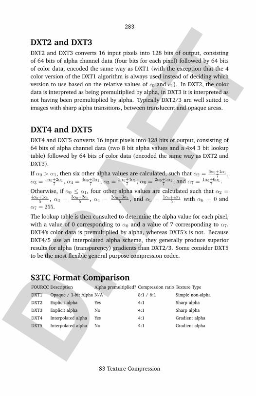
DRAF

T

283


DXT2 and DXT3DXT2 and DXT3 converts 16 input pixels into 128 bits of output, consistingof 64 bits of alpha channel data (four bits for each pixel) followed by 64 bitsof color data, encoded the same way as DXT1 (with the exception that the 4color version of the DXT1 algorithm is always used instead of deciding whichversion to use based on the relative values of c0 and c1). In DXT2, the colordata is interpreted as being premultiplied by alpha, in DXT3 it is interpreted asnot having been premultiplied by alpha. Typically DXT2/3 are well suited toimages with sharp alpha transitions, between translucent and opaque areas.

DXT4 and DXT5DXT4 and DXT5 converts 16 input pixels into 128 bits of output, consisting of64 bits of alpha channel data (two 8 bit alpha values and a 4x4 3 bit lookuptable) followed by 64 bits of color data (encoded the same way as DXT2 andDXT3).

If α0 > α1, then six other alpha values are calculated, such that α2 = 6α0+1α17 ,

α3 = 5α0+2α17 , α4 = 4α0+3α1

7 , α5 = 3α0+4α17 , α6 = 2α0+5α1

7 , and α7 = 1α0+6α17 .

Otherwise, if α0 ≤ α1, four other alpha values are calculated such that α2 =4α0+1α1

5 , α3 = 3α0+2α15 , α4 = 2α0+3α1

5 , and α5 = 1α0+4α15 with α6 = 0 and

α7 = 255.

The lookup table is then consulted to determine the alpha value for each pixel,with a value of 0 corresponding to α0 and a value of 7 corresponding to α7.DXT4’s color data is premultiplied by alpha, whereas DXT5’s is not. BecauseDXT4/5 use an interpolated alpha scheme, they generally produce superiorresults for alpha (transparency) gradients than DXT2/3. Some consider DXT5to be the most flexible general purpose compression codec.

S3TC Format ComparisonFOURCC Description Alpha premultiplied? Compression ratio Texture Type

DXT1 Opaque / 1-bit Alpha N/A 8:1 / 6:1 Simple non-alpha

DXT2 Explicit alpha Yes 4:1 Sharp alpha

DXT3 Explicit alpha No 4:1 Sharp alpha

DXT4 Interpolated alpha Yes 4:1 Gradient alpha

DXT5 Interpolated alpha No 4:1 Gradient alpha

DRAF

T

284

Scanline rendering

See also

• →3Dc• FXT1• DirectDraw Surface

External links

• NVIDIA Texture Tools303

• ATI Developer: Tools304

• MSDN Compressed Texture Resources305

• Comparison between S3TC and FXT1 texture compression306

• The Truth about S3TC307 Note: This article used an early S3TC compressionengine, not nVidia’s or ATI’s updated codecs.

Source: http://en.wikipedia.org/wiki/S3_Texture_Compression

Principal Authors: Timharwoodx, NJM, Paul-Jan, N00body, Ilya K

Scanline rendering

Scanline rendering is a rendering technique, or family of algorithms, in →3Dcomputer graphics that works on a row-by-row basis rather than a polygon-by-polygon or pixel-by-pixel basis. All of the polygons to be rendered are firstsorted by the top y coordinate at which they first appear, then each row orscan line of the image is computed using the intersection of a scan line withthe polygons on the front of the sorted list, while the sorted list is updated todiscard no-longer-visible polygons as the active scan line is advanced down thepicture.

The asset of this method is that it is not necessary to translate the coordinatesof all vertices from the main memory into the working memory—only vertices

http://developer.nvidia.com/object/nv_texture_tools.html303

http://www.ati.com/developer/tools.html304

http://msdn.microsoft.com/library/default.asp?url=/library/en-us/directx9_c/directx/graphics/Pro-305

grammingGuide/GettingStarted/Direct3DTextures/compressed/compressedtextureresources.asphttp://www.digit-life.com/articles/reviews3tcfxt1/306

http://web.archive.org/web/20030618083605/www.hardwarecentral.com/hardwarecentral/reports307

/140/1/

DRAF

T

285

Scanline rendering

defining edges that intersect the current scan line need to be in active memory,and each vertex is read in only once. The main memory is often very slow com-pared to the link between the central processing unit and cache memory, andthus avoiding re-accessing vertices in main memory can provide a substantialspeedup.

This kind of algorithm can be easily integrated with the →Phong reflectionmodel, the Z-buffer algorithm, and many other graphics techniques.

Scanline rendering is used by most modern graphics cards and is typically ac-cessed by the programmer using some 3D API such as→OpenGL or→Direct3D.

HistoryThe first publication of the scanline rendering technique was probably byWylie, Romney, Evans, and Erdahl in 1967.308

Other early developments of the scanline rendering method were by Bouknightin 1969,309 and Newell, Newell, and Sancha in 1972.310 Much of the early workon these methods was done in Ivan Sutherland’s graphics group at the Univer-sity of Utah, and at the Evans & Sutherland company in Salt Lake City, Utah.

References

External Links[http://accad.osu.edu/~waynec/history/tree/utah.html University of UtahGraphics Group History

See also

• Scan line• Pixel• Raster scan

Source: http://en.wikipedia.org/wiki/Scanline_rendering

Principal Authors: Dicklyon, Samwisefoxburr, Nixdorf, Kc9cqj, Timo Honkasalo

Wylie, C, Romney, G W, Evans, D C, and Erdahl, A, "Halftone Perspective Drawings by Computer,"308

Proc. AFIPS FJCC 1967, Vol. 31, 49Bouknight W.J, "An Improved Procedure for Generation of Half-tone Computer Graphics Representa-309

tion," UI, Coordinated Science Laboratory, Sept 1969Newell, M E, Newell R. G, and Sancha, T.L, "A New Approach to the Shaded Picture Problem," Proc310

ACM National Conf. 1972

DRAF

T

286

Scene graph

Scene graph

A scene-graph is a general data structure commonly used by vector-basedgraphics editing applications and modern computer games. Examples of suchprograms include AutoCAD, Adobe Illustrator and CorelDRAW.

The scene-graph is an object-oriented structure that arranges the logical andoften (but not necessarily) spatial representation of a graphical scene. Thedefinition of a scene-graph is fuzzy, due to the fact that programmers whoimplement scene-graphs in applications and in particular the games industrytake the basic principles and adapt these to suit a particular application. Thismeans there is no hard and fast rule what a scene-graph should be or shouldn’tbe.

Scene-graphs are a collection of nodes in a graph or tree structure. This meansthat a node may have many children but often only a single parent, the effectof a parent is apparent to all its child nodes - An operation applied to a groupautomatically propagates its effect to all of its members. In many programs,associating a geometrical transformation matrix (see also transformation andmatrix) at each group level and concatenating such matrices together is anefficient and natural way to process such operations. A common feature, forinstance, is the ability to group related shapes/objects into a compound objectwhich can then be moved, transformed, selected, etc. as easily as a singleobject.

Scene-graphs in graphics editing toolsIn vector-based graphics editing, each node in a scene graph represents someatomic unit of the document, usually a shape such as an ellipse or Bezier path.Although shapes themselves (particularly paths) can be decomposed furtherinto nodes such as spline nodes, it is practical to think of the scene graph ascomposed of shapes rather than going to a lower level of representation.

Another useful and user-driven node concept is the layer. A layer acts like atransparent sheet upon which any number of shapes and shape groups canbe placed. The document then becomes a set of layers, any of which can beconveniently made invisible, dimmed, and/or locked (made read-only). Someapplications place all layers in a linear list while others support sublayers (i.e.,layers within layers, to any desired depth).

Internally, there may be no real structural difference between layers and groupsat all, since they are both just nested scenegraphs. If differences are needed,a common type declaration in C++ would be to make a generic scenegraph

DRAF

T

287

Scene graph

class, and then derive layers and groups as subclasses. A visibility member, forexample, would be a feature of a layer but not necessarily of a group.

Scene-graphs in games and 3D applicationsScene graphs are ideal for modern games using 3D graphics and increasinglylarge worlds or levels. In such applications, nodes in a scene-graph (generally)represent entities or objects in the scene.

For instance, a game might define a logical relationship between a knight anda horse so that the knight is considered an extension to the horse. The scenegraph would have a ’horse’ node with a ’knight’ node attached to it.

As well as describing the logical relationship, the scene-graph may also describethe spatial relationship of the various entities: the knight moves through 3Dspace as the horse moves.

In these large applications, memory requirements are major considerationswhen designing a scene-graph. For this reason many large scene-graph sys-tems use instancing to reduce memory costs and increase speed. In our exam-ple above, each knight is a separate scene node, but the graphical represen-tation of the knight (made up of a 3D mesh, textures, materials and shaders)is instanced. This means that only a single copy of the data is kept, which isthen referenced by any ’knight’ nodes in the scene-graph. This allows a reducedmemory budget and increased speed, since when a new knight node is created,the appearance data does not need to be duplicated.

Scene-graph ImplementationThe simplest form of scene graph uses an array or linked list data structure, anddisplaying its shapes is simply a matter of linearly iterating the nodes one byone. Other common operations, such as checking to see which shape intersectsthe mouse pointer (e.g., in a GUI-based applications) are also done via linearsearches. For small scenegraphs, this tends to suffice.

Larger scenegraphs cause linear operations to become noticeably slow and thusmore complex underlying data structures are used, the most popular being atree. This is the most common form of scene-graph. In these scene-graphs thecomposite design pattern is often employed to create the hierarchical represen-tation of group-nodes and leaf-nodes.

Group Nodes - Can have any number of child nodes attached to it. Groupnodes includes transformations and switch nodes.

DRAF

T

288

Scene graph

Leaf Nodes - Are nodes that are actually rendered or see the effect of an oper-ation. These include objects, sprites, sounds, lights and anything that could beconsidered ’rendered’ in some abstract sense.

Scene-graph Operations and DispatchIn order to apply an operation to a scene-graph some way of dispatching anoperation based upon what node is currently being considered is needed. Forexample in a render operation a transformation group-node would do nothingmore than accumulate its transformation (generally this is matrix multiplica-tion but could involve operations with vector displacement and quaternions orEuler angles instead). Whereas an object leaf-node would send the object offfor rendering to the renderer (some implementations might render the objectdirectly but this can integrate the underlying rendering API - e.g. OpenGL orDirectX too tightly and rigidly - it is better to separate the scene-graph andrenderer systems as this promotes good OOP style and extensibility).

In order to dispatch differently for different node types several different ap-proaches can be taken, each have pros and cons and are widely disputed amongprogrammers arguing which is best.

In Object-Oriented languages such as C++ this can easily be achieved by virtu-al functions, the node base class has virtual functions for every operation thatcan be performed on the nodes. This is simple to do but prevents the additionof new operations by other programmers that don’t have access to the source.

Alternatively the visitor pattern can be used - this is relatively simple andfaster than virtual functions where the operation to be performed is decided bymultiple dispatch. This has a similar disadvantage in that it is similarly difficultto add new node types.

Other techniques involve the use of RTTI (Run-Time-Type-Information) the op-eration can be realised as a class which is passed the current node, it thenqueries the nodes type (RTTI) and looks up the correct operation in an array ofcallbacks or functors. This requires that at initialisation the user/system regis-ters functors/callbacks with the different operations so they can be looked upin the array. This system offers massive flexibility, speed and extensibility ofnew nodes and operations.

Variations on these techniques exist and new methods can offer added benefits- one alternative is scene-graph re-building where the scene-graph is re-built foreach of the operations performed, this however can be very slow but producesa highly optimised scene-graph. This demonstrates that a good scene-graphimplementation depends heavily on the application it is used in.

DRAF

T

289

Scene graph

TraversalsTraversals are the key to the power of applying operations to scene-graphs. Atraversal generally consists of starting at some arbitrary node (often the root ofthe scene-graph), applying the operation(s) often the updating and renderingoperations are applied one after the other, and recursively moving down thescene-graph(tree) to the child nodes, until a leaf node is reached. At this pointmany scene-graphs then traverse back up the tree possibly applying a simi-lar operation. As an example - Rendering: While recursively traversing downthe scene-graph hierarchy the operations applies a PreRender operation, oncereaching a leaf node it begin traversing back up the tree applying a PostRenderoperation - This nicely allows certain nodes push a state for child nodes andpop the state afterward.

Some scene-graph operations are actually more efficient when nodes are tra-versed in a different order - This is where some systems implement scene-graphre-building to reorder the scene-graph into an easier to parse format or tree.

For example:

In 2D cases, scenegraphs typically render themselves by starting at the tree’sroot node and then recursively drawing the child nodes. The tree’s leavesrepresent the most foreground objects. Since drawing proceeds from back tofront with closer objects simply overwriting farther ones, the process is knownas employing the →Painter’s algorithm. In 3D systems, which often employdepth buffers, it is more efficient to draw the closest objects first, since fartherobjects often need only be depth-tested instead of actually rendered.

Scene-graph and Bounding Volume Hierarchies (BVHs)Bounding Volume Hierarchies (BVHs) are useful for numerous tasks - includingefficient culling and speeding up collision detection between objects. A BVHis a spatial structure but doesn’t have to partition the geometry (see spatialpartitioning, below).

A BVH is a tree of bounding volumes (often spheres, AABBs or/and OBBs).At the bottom of the hierarchy the size of the volume is just large enough toencompass a single object tightly (or possibly even some smaller fraction of anobject in high resolution BVHs), as you walk up the hierarchy each node hasits own volume which tightly encompasses all the volumes beneath it. At theroot of the tree is a volume that encompasses all the volumes in the tree (thewhole scene).

BVHs are useful for speeding up collision detection between objects. If anobject’s bounding volume does not intersect a volume higher in the tree then

DRAF

T

290

Scene graph

it cannot intersect any object below that node (so they are all rejected veryquickly).

Obviously there are some similarities between BVHs and scene-graphs. Ascene-graph can easily be adapted to include/become a BVH - if each node hasa volume associated or there’s purpose built ’bound node’ added in at conve-nient location in the hierarchy. This may not be the typical view of scene-graphbut there are benefits to including a BVH in a scene-graph.

Scene-graphs and Spatial PartitioningAn effective way of combining spatial partitioning and scene-graphs is by cre-ating a scene leaf node that contains the spatial partitioning data - This data isusually static and generally contains non-moving level data in some partitionedform. Some systems may have the systems separate and render them separate-ly, this is fine and there are no real advantages to either method. In particularit is bad to have the scene-graph contained within the spatial partitioning sys-tem, this is because the scene-graph is better thought of as the grander systemto the spatial partitioning.

When it is useful to combine themIn short: Spatial partitioning will/should considerably speed up the processingand rendering time of the scene-graph.

Very large drawings, or scene graphs that are generated solely at runtime (ashappens in ray tracing rendering programs), require defining of group nodesin a more automated fashion. A raytracer, for example, will take a scene de-scription of a 3D model and build an internal representation that breaks up itsindividual parts into bounding boxes (also called bounding slabs). These boxesare grouped hierarchically so that ray intersection tests (as part of visibility de-termination) can be efficiently computed. A group box that does not intersectan eye ray, for example, can entirely skip having to test any of its members.

A similar efficiency holds in 2D applications as well. If the user has magnifieda document so that only part of it is visible on his computer screen, and thenscrolls said document, it is useful to use a bounding box (or in this case, abounding rectangle scheme) to quickly determine which scenegraph elementsare visible and thus actually need to be drawn.

Depending on the particulars of the application’s drawing performance, a largepart of the scenegraph’s design can be impacted by rendering efficiency con-siderations. In 3D video games such as Quake, for example, binary space par-titioning (BSP) trees are heavily favored to minimize visibility tests. BSP trees,

DRAF

T

291

Scene graph

however, take a very long time to compute from design scenegraphs, and mustbe recomputed if the design scenegraph changes so the levels tend to remainstatic and dynamic characters aren’t generally considered in the spatial parti-tioning scheme.

Scenegraphs for dense regular objects such as heightfields and polygon meshestend to employ quadtrees and octrees, which are specialized variants of a 3Dbounding box hierarchy. Since a heightfield occupies a box volume itself, recur-sively subdividing this box into eight subboxes (hence the ’oct’ in octree) untilindividual heightfield elements are reached is efficient and natural. A quadtreeis simply a 2D octree.

PHIGSPHIGS was the first commercial scene-graph specification, and became an ANSIstandard in 1988. Disparate implementations were provided by Unix hardwarevendors. The "HOOPS 3D Graphics System"311 appears to have been the firstcommercial scene graph library provided by a single software vendor. It wasdesigned to run on disparate lower-level 2D and 3D interfaces, with the firstmajor production version (v3.0) completed in 1991. Shortly thereafter, SiliconGraphics released IRIS Inventor 1.0 (1992), which was a scene-graph built ontop of the IRIS GL 3D API. It was followed up with →Open Inventor in 1994,a portable scene graph built on top of OpenGL. More 3D scenegraph librariescan be found in 3D Scenegraph APIs.

References

Books

• Leler, Wm and Merry, Jim (1996) 3D with HOOPS, Addison-Wesley• Wernecke, Josie (1994) The Inventor Mentor: Programming Object-

Oriented 3D Graphics with Open Inventor, Addison-Wesley, ISBN 0-201-62495-8 (Release 2)

Web sites and articles

• Strauss, Paul (1993). "IRIS Inventor, a 3D Graphics Toolkit"312

• Helman, Jim; Rohlf, John (1994). "IRIS Performer: A High PerformanceMultiprocessing Toolkit for Real-Time 3D Graphics"313

http://www.hoops3d.com311



DRAF

T

292

Shader

• Carey, Rikk and Bell, Gavin (1997). "The Annotated VRML 97 ReferenceManual"314

• PEXTimes 315

• Bar-Zeev, Avi. "Scenegraphs: Past, Present, and Future"316

• Open Scene Graph317

• OpenSG318

Source: http://en.wikipedia.org/wiki/Scene_graph

Principal Authors: Mortene, Mikkalai, Tommstein, CamTarn, WillC2 45220, Reinyday, Engwar

Shader

A shader is a computer program used in →3D computer graphics to determinethe final surface properties of an object or image. This often includes arbitrarilycomplex descriptions of light absorption, diffusion, texture mapping, reflection,refraction, shadowing, surface displacement and post-processing effects.

By design, shaders are ideal candidates for parallel execution by multiplegraphic processors, which are usually located on a video card, allowing forscalable multiprocessing and lessening the burden on the CPU for renderingscenes.

Because of the goals shaders are designed to address, they are usually writ-ten using a shading language, a specifically designed programming languagebuilt around the intrinsic strengths and weaknesses of the different compu-tational model. Although limited in some ways when compared to tradition-al approaches, the parallel architecture exposed by shaders has been used tocombine highly scalable processing power with the flexibility of programmabledevices, which is a boon in addressing the growing demands for graphics qual-ity.

The increasing performance and programmability of shader-based architec-tures attracted researchers trying to exploit the new parallel model for GeneralPurpose computation on GPUs. This demonstrated that shaders could be used

http://www.jwave.vt.edu/~engineer/vrml97book/ch1.htm314

http://www.jch.com/jch/vrml/PEXTimes.txt315

http://www.realityprime.com/scenegraph.php316

http://www.openscenegraph.org317

http://www.opensg.org318

DRAF

T

293

Shader

to process a large variety of information, and not just rendering-specific tasks.This new programming model, which resembles stream processing, allows highcomputational rates at extremely low cost that will operate on wide installedbase (e.g. the common home PC).

Real-time Shader StructureThere are different approaches to shading, mainly because of the various appli-cations of the targeted technology. Production shading languages are usuallyat a higher abstraction level, avoiding the need to write specific code to handlelighting or shadowing. In contrast, real-time shaders integrate light and shad-owing computations. In those languages, the lights are passed to the shaderitself as parameters.

There are actually two different applications of shaders in real-time shadinglanguages. Although the feature set actually converged (so it’s possible to writea vertex shader using the same functions of a fragment shader), the differentpurposes of computation impose limitations to be acknowledged.

Vertex ShadersVertex shaders are applied for each vertex and run on a programmable vertexprocessor. Vertex shaders define a method to compute vector space transfor-mations and other linearizable computations.

A vertex shader expects various inputs:

• Uniform variables are constant values for each shader invocation. It is al-lowed to change the value of each uniform variable between different shad-er invocation batches. This kind of variable is usually a 3-component arraybut this does not need to be. Usually, only basic datatypes are allowed tobe loaded from external APIs so complex structures must be broken down.Uniform variables can be used to drive simple conditional execution on aper-batch basis. Support for this kind of branching at a vertex level hasbeen introduced in shader model 2.0.

• Vertex attributes, which are a special case of variant variables, which areessentially per-vertex data such as vertex positions. Most of the time, eachshader invocation performs computation on different data sets. The exter-nal application usually does not access these variables "directly" but man-ages as large arrays. Besides this little detail, applications are usually ca-pable of changing a single vertex attribute with ease. Branching on vertexattributes requires a finer degree of control which is supported with extend-ed shader model 2.

DRAF

T

294

Shader

Vertex shader computations are meant to provide following stages of the graph-ics pipeline with interpolable fragment attributes. Because of this, a vertexshader must output at least the transformed homogeneous vertex position (inGLSL this means the variable gl_Position must be written). Outputs from differ-ent vertex shader invocations from the same batch will be linearly interpolatedacross the primitive being rendered. The result of this linear interpolation isfetched to the next pipeline stage.

Some examples of vertex shader’s functionalities include arbitrary mesh de-formation (possibly faking lens effects such as fish-eye) and vertex displace-ments in general, computing linearizable attributes for later pixel-shaders suchas texture coordinate transformations. Actually, vertex shaders cannot createvertices.

Pixel ShadersPixel shaders are used to compute properties which, most of the time, arerecognized as pixel colors.

Pixel shaders are applied for each pixel. They are run on a pixel processor,which usually features much more processing power than its vertex-orientedcounterpart. As of October 2005, some architectures are merging the two pro-cessors in a single one to increase transistor usage and provide some kind ofload balancing.

As previously stated, the pixel shaders expects input from interpolated vertexvalues. This means there are three sources of information:

• Uniform variables can still be used and provide interesting opportunities.A typical example is passing an integer providing a number of lights tobe processed and an array of light parameters. Textures are special casesof uniform values and can be applied to vertices as well, although vertextexturing is often more expensive.

• Varying attributes is a special name to indicate fragment’s variant variables,which are the interpolated vertex shader output. Because of their origin, theapplication has no direct control on the actual value of those variables.

Branching on the pixel processor has also been introduced with an extendedpixel shader 2 model but hardware supporting this efficiently is beginning to becommonplace only now (6 March 2006), usually with full pixel shader model3 support.

A fragment shader is allowed to discard the results of its computation, meaningthat the corresponding framebuffer position must retain its actual value.

DRAF

T

295

Shader

Fragment shaders also don’t need to write specific color information becausethis is not always wanted. Not producing color output when expected howevergives undefined results in GLSL.

Fragment shaders have been employed to apply accurate lighting models, sim-ulate multi-layer surface properties, simulating natural phenomena such as tur-bulence (vector field simulations in general) and applying depth of field to ascene or other color-space transformations.

TexturingNote: the following information on texture mapping with shaders appliesspecifically to →GLSL. Those statements may not hold true for DirectX HLSL.

The functionality by itself continues to be applied "as usual" with shading lan-guages providing special ad-hoc functions and opaque objects.

It has been stated that textures are special uniform variables. The shading lan-guages define special variables to be used as textures called samplers. Eachsampler does have a specific lookup mode assigned explicitly in the name.Looking up a texture actually means to get an interpolated texel color at aspecified position. For example, in GLSL sampler2D will access a specific tex-ture performing bidimensional texturing and filtering to be used with a tex2Dfunction call. Other details are specified by the function used to actually per-form the lookup. For cube map textures, a samplerCube would be used witha textureCube function call.

Understanding completely the model also needs to know a little about the pre-vious shading model, commonly referred as multitexturing or texture cascade.For our purposes, we’ll just assume there is a limited set of units which can belinked to specific textures and somehow produce color results, possibly combin-ing them in a sequential order. This is redundant with the new programmingmodel which allows much greater flexibility.

To lookup to a specific texture, the sampler really needs to know what of thosetexture units needs to be used with the specified lookup mode. This meanssamplers are really integers referring to the texture unit used to carry on thelookup. It will now be possible to bind to each texture unit an image texturejust as usual. It will happen that those units are actually a subset of "legacy"texture units and are referred as image units. Most implementation actuallyallow more image units than texture units because of the lower complexity toimplement them but also to push for the new programming model. In short,samplers are really linked to image units, which are bound to textures.

DRAF

T

296

Shader

For final users, this extra flexibility results in both improved performance andricher content because of the better hardware utilization and resources.

Lighting & ShadowingConsidering the lighting equation, we have seen the trend to move evaluationsto fragment granularity. Initially, the lighting computations were performedat vertex level (phong lighting model) but improvements in fragment proces-sor designs allowed to evaluate much more complex lighting equations suchas the blinn lighting model, often referred as bump mapping. In this lattertechnique, vertex shaders are used to set up a vertex local space (also calledtangent space) which is then used to compute per-pixel lighting vectors. Theactual math for this can be quite involved and is beyond the scope of this arti-cle.

It is well acknowledged that lighting really needs hardware support for dynam-ic loops (this is often referred as DirectX Pixel Shader Model 3.0) because thisallows to process many lights of the same type with a single shader. By con-trast, previous shading models would have need the application to use multipass rendering (an expensive operation) because of the fixed loops. This ap-proach would also have needed more complicated machinery. For example,after finding there are 13 "visible" lights, the application would have the needto use a shader to process 8 lights (suppose this is the upper hardware limi-tation) and another shader to process the remaining 5. If there are 7 lightsthe application would have needed a special 7-light shader. By contrast, withdynamic loops the application can iterate on dynamic variables thus defininga uniform array to be 13 (or 7) "lights long" and get correct results, provid-ed this actually fits in hardware capabilities. At the time this is being written(27 October 2005) there are enough resources to evaluate over 50 lights perpass when resources are managed carefully. Compare this to old programmingmodels.

Computing accurate shadows make this much more complicated, depending onthe algorithm used. Compare stencil shadow volumes and shadow mapping. Inthe first case, the algorithm requires at least some care to be applied to multiplelights at once and there’s no actual proof of a multi-light shadow volume basedversion. Shadow mapping by contrast seems to be much more well suitedto future hardware improvements and to the new shading model which alsoevaluates computations at fragment level. Shadow maps however needs to bepassed as samplers, which are limited resources: actual hardware (27 October2005) support up to 16 samplers so this is a hard-limit, unless some tricks are

DRAF

T

297

Shader

used. It is speculated that future hardware improvements and packing multipleshadow maps in a single 3D-texture will rapidly raise this resource availability.

Further reading

• Steve Upstill: The RenderMan Companion: A Programmer’s Guide to Real-istic Computer Graphics, Addison-Wesley, ISBN 0-201-50868-0

• David S. Elbert, F. Kenton Musgrave, Darwyn Peachey, Ken Perlin, StevenWorley: Texturing and modeling: a procedural approach, AP Professional,ISBN 0-12-228730-4. Ken Perlin is the author of →Perlin noise, an impor-tant procedural texturing primitive.

• Randima Fernando, Mark Kilgard. The Cg Tutorial: The Definitive Guideto Programmable Real-Time Graphics, Addison-Wesley Professional, ISBN0-32119-496-9

• Randi Rost: OpenGL Shading Language, Addison-Wesley Professional, ISBN0-321-19789-5

References

1. ↑ Search ARB_shader_objects319 for the issue "32) Can you explain how uni-form loading works?". This is an example of how a complex data structuremust be broken in basic data elements.

2. ↑ Required machinery has been introduced in OpenGL byARB_multitexture320 but this specification is no more available since itsintegration in core OpenGL 1.2.

3. ↑ Search again ARB_shader_objects321 for the issue "25) How are samplersused to access textures?". You may also want to check out "Subsection2.14.4 Samplers".

4. ↑ Search NVIDIA developer resources322 for various papers on per-pixellighting.

5. ↑ You’ll be glad to see those limits are (at least theorically) rather high.Check out The OpenGL R© Shading Language323 for the string "52) Howshould resource limits for the shading language be defined?" and look foryour favorite video card at Delphi3d.net hardware database324.

http://oss.sgi.com/projects/ogl-sample/registry/ARB/shader_objects.txt319

http://oss.sgi.com/projects/ogl-sample/registry/ARB/multitexture.txt320

http://oss.sgi.com/projects/ogl-sample/registry/ARB/shader_objects.txt321

http://developer.nvidia.com322

http://www.opengl.org/documentation/glsl/323

http://www.delphi3d.net/hardware/index.php324

DRAF

T

298

Shading language

Source: http://en.wikipedia.org/wiki/Shader

Principal Authors: T-tus, Flamurai, MaxDZ8, Parameter, Rufous

Shading language

A shading language is a special programming language adapted to easily mapon shader programming. Those kind of languages usually have special da-ta types like color and normal. Because of the various target markets of 3Dgraphics, different shading languages have been developed: a brief overview isgiven below.

Production renderingThese kind of shading languages are geared towards maximum image quali-ty. Material properties are totally abstracted, little programming skill and nohardware knowledge is required. These kind of shaders are often developed byartists to get the right "look", just as texture mapping, lighting and other facetsof their work.

Processing these kinds of shaders is usually a time-consuming process. Thecomputational power required to get this kind of shading to work can be ratherexpensive because of their ability to produce photorealistic results. Most of thetime, production rendering is run on large computer clusters.

RenderMan Shading LanguageRenderMan Shading Language, which is defined in the RenderMan InterfaceSpecification , is the most common shading language for production-qualityrendering. RenderMan by Rob Cook, is currently used in all of Pixar’s products.It’s also one of the first shading languages ever implemented.

The language actually defines six major shader types:

• Light source shaders compute the color of the light emitted from a point onthe light source towards a point on the surface being illuminated.

• Surface shaders are used to model the optical properties of the object be-ing illuminated. They output the final color and position of the point be-ing illuminated by taking into account the incoming light and the physicalproperties of the object.

DRAF

T

299

Shading language

• Displacement shaders manipulate the surface’s geometry independent of itscolor.

• Deformation shaders transform the entire space that a geometry is definedin. Only one RenderMan implementation, the AIR renderer, actually imple-ments this shader type.

• Volume shaders manipulate the color of a light as it passes through a vol-ume. They are used to create effects like fog.

• Imager shaders describe a color transformation to final pixel values. Thisis much like an image filter, however the imager shader operates on pre-quantized data, which typically has a greater dynamic range than can bedisplayed on the output device.

Most of the time RenderMan is referenced, it is really meant to speak aboutPRMan, the RenderMan implementation from Pixar, which was the only oneavailable for years. Further information can be found at the RenderManrepository325.

Gelato Shading LanguageDeveloped by NVIDIA, a graphics processing unit manufacturer for its Gelatorendering software.

This language is meant to interact with hardware, providing higher computa-tional rates while retaining cinematic image quality and functionalities.

Real-time renderingUntil recently, developers did not have the same level of control over the out-put from the graphics pipeline of graphics cards, but shading languages forreal-time rendering are now widespread. They provide both higher hardwareabstraction and a more flexible programming model when compared to previ-ous paradigms which hardcoded transformation and shading equations. Thisresults in both giving the programmer greater control over the rendering pro-cess, and delivering richer content at lower overhead.

Quite surprisingly those shaders, which are designed to be executed directlyon the GPU at the proper point in the pipeline for maximum performance, alsoscored successes in general processing because of their stream programmingmodel.

http://www.renderman.org/325

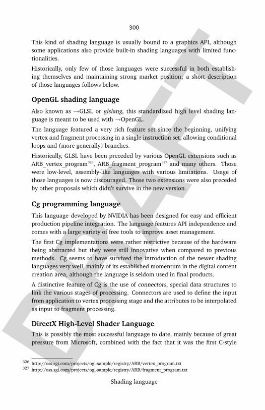
DRAF

T

300

Shading language

This kind of shading language is usually bound to a graphics API, althoughsome applications also provide built-in shading languages with limited func-tionalities.

Historically, only few of those languages were successful in both establish-ing themselves and maintaining strong market position; a short descriptionof those languages follows below.

OpenGL shading language

Also known as →GLSL or glslang, this standardized high level shading lan-guage is meant to be used with →OpenGL.

The language featured a very rich feature set since the beginning, unifyingvertex and fragment processing in a single instruction set, allowing conditionalloops and (more generally) branches.

Historically, GLSL have been preceded by various OpenGL extensions such asARB_vertex_program326, ARB_fragment_program327 and many others. Thosewere low-level, assembly-like languages with various limitations. Usage ofthose languages is now discouraged. Those two extensions were also precededby other proposals which didn’t survive in the new version.


This language developed by NVIDIA has been designed for easy and efficientproduction pipeline integration. The language features API independence andcomes with a large variety of free tools to improve asset management.

The first Cg implementations were rather restrictive because of the hardwarebeing abstracted but they were still innovative when compared to previousmethods. Cg seems to have survived the introduction of the newer shadinglanguages very well, mainly of its established momentum in the digital contentcreation area, although the language is seldom used in final products.

A distinctive feature of Cg is the use of connectors, special data structures tolink the various stages of processing. Connectors are used to define the inputfrom application to vertex processing stage and the attributes to be interpolatedas input to fragment processing.

DirectX High-Level Shader LanguageThis is possibly the most successful language to date, mainly because of greatpressure from Microsoft, combined with the fact that it was the first C-style

http://oss.sgi.com/projects/ogl-sample/registry/ARB/vertex_program.txt326

http://oss.sgi.com/projects/ogl-sample/registry/ARB/fragment_program.txt327

DRAF

T

301

Shading language

shader language to be used for real-time rendering. The high level shaderlanguage (also called HLSL for short) was released before its main competitor,GLSL, although its feature set was later extended in two different revisions tomatch the GLSL feature set.

References

1. ↑ https://renderman.pixar.com/products/rispec/2. ↑ NVIDIA Gelato official website, http://film.nvidia.com/page/gelato.html3. ↑ Official language specification, http://www.opengl.org/documentation

/glsl/4. ↑ Previous vertex shading languages (in no particular order) for

OpenGL include EXT_vertex_shader328, NV_vertex_program329, theaforementioned ARB_vertex_program330, NV_vertex_program2331 andNV_vertex_program3332.

5. ↑ For fragment shading nvparse333 is possibly the first shading lan-guage featuring high-level abstraction based on NV_register_combiners334,NV_register_combiners2335 for pixel math and NV_texture_shader336,NV_texture_shader2337 and NV_texture_shader3338 for texture lookups.ATI_fragment_shader339 did not even provide a "string orient-ed" parsing facility (although it has been later added byATI_text_fragment_shader340). ARB_fragment_program341, has been verysuccessful. NV_fragment_program342 and NV_fragment_program2343 areactually similar although the latter provides much more advanced func-tionality in respect to others.

http://oss.sgi.com/projects/ogl-sample/registry/EXT/vertex_shader.txt328

http://oss.sgi.com/projects/ogl-sample/registry/NV/vertex_program.txt329

http://oss.sgi.com/projects/ogl-sample/registry/ARB/vertex_program.txt330

http://oss.sgi.com/projects/ogl-sample/registry/NV/vertex_program2.txt331

http://oss.sgi.com/projects/ogl-sample/registry/NV/vertex_program3.txt332

http://developer.nvidia.com/object/nvparse.html333

http://oss.sgi.com/projects/ogl-sample/registry/NV/register_combiners.txt334

http://oss.sgi.com/projects/ogl-sample/registry/NV/register_combiners2.txt335

http://oss.sgi.com/projects/ogl-sample/registry/NV/texture_shader.txt336

http://oss.sgi.com/projects/ogl-sample/registry/NV/texture_shader2.txt337

http://oss.sgi.com/projects/ogl-sample/registry/NV/texture_shader3.txt338

http://oss.sgi.com/projects/ogl-sample/registry/ATI/fragment_shader.txt339

http://oss.sgi.com/projects/ogl-sample/registry/ATI/text_fragment_shader.txt340

http://oss.sgi.com/projects/ogl-sample/registry/ARB/fragment_program.txt341

http://oss.sgi.com/projects/ogl-sample/registry/NV/fragment_program.txt342

http://oss.sgi.com/projects/ogl-sample/registry/NV/fragment_program2.txt343

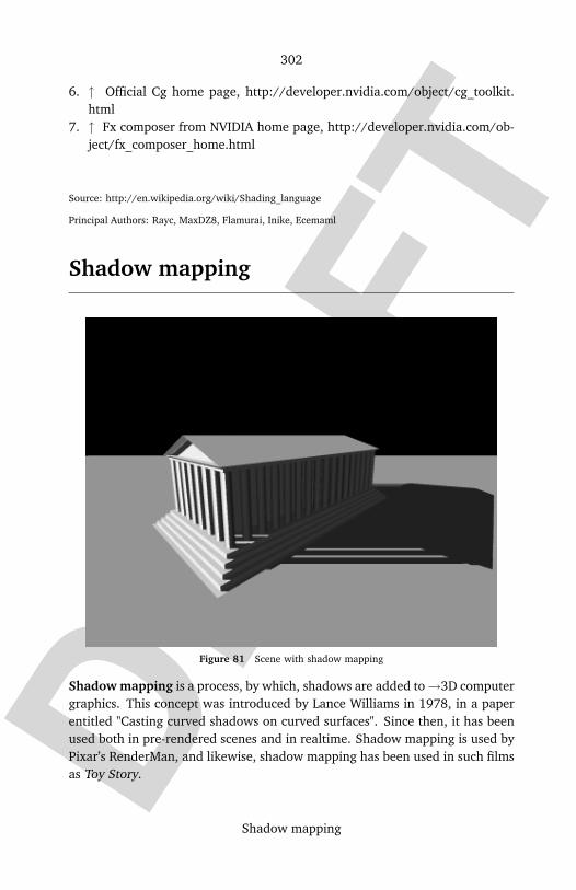
DRAF

T

302

Shadow mapping

6. ↑ Official Cg home page, http://developer.nvidia.com/object/cg_toolkit.html

7. ↑ Fx composer from NVIDIA home page, http://developer.nvidia.com/ob-ject/fx_composer_home.html

Source: http://en.wikipedia.org/wiki/Shading_language

Principal Authors: Rayc, MaxDZ8, Flamurai, Inike, Ecemaml

Shadow mapping

Figure 81 Scene with shadow mapping

Shadow mapping is a process, by which, shadows are added to→3D computergraphics. This concept was introduced by Lance Williams in 1978, in a paperentitled "Casting curved shadows on curved surfaces". Since then, it has beenused both in pre-rendered scenes and in realtime. Shadow mapping is used byPixar’s RenderMan, and likewise, shadow mapping has been used in such filmsas Toy Story.

DRAF

T

303

Shadow mapping

Figure 82 Scene with no shadows

Shadows are created by testing whether a pixel is visible from the light source,by comparing it to a z-buffer or depth image, in the form of a texture. Thistechnique involves three passes or re-renderings, although it can be accom-plished with just two.

Principle of a shadow and a shadow mapA shadow can be considered thus: Imagine you have a spot light source, that isaimed at some objects. The shadow thus cast by this light source can be visual-ized by viewing through the light source at the objects and marking the visibleareas, and disregarding every point not seen by the light source as "shadow".

The complexity of this simple operation becomes apparent when one consid-ers the amount of photons that are incident on the surface of the objects. Thesheer number of photons incident cannot be simulated at real-time even bycurrent fastest computers. Hence to make this effect more accessible to peoplevia games, 3D modelling tools, visualization tools, etc, programmers employa number of techniques to fake this complex shadow operation. The follow-ing is a partial list of algorithms that most programmers use to approach thisproblem:

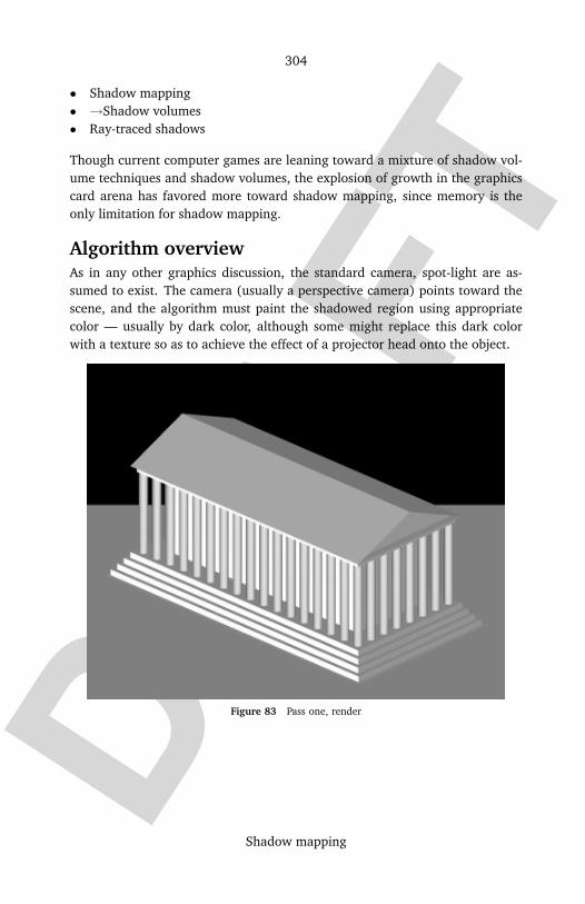
DRAF

T

304

Shadow mapping

• Shadow mapping• →Shadow volumes• Ray-traced shadows

Though current computer games are leaning toward a mixture of shadow vol-ume techniques and shadow volumes, the explosion of growth in the graphicscard arena has favored more toward shadow mapping, since memory is theonly limitation for shadow mapping.

Algorithm overviewAs in any other graphics discussion, the standard camera, spot-light are as-sumed to exist. The camera (usually a perspective camera) points toward thescene, and the algorithm must paint the shadowed region using appropriatecolor — usually by dark color, although some might replace this dark colorwith a texture so as to achieve the effect of a projector head onto the object.

Figure 83 Pass one, render

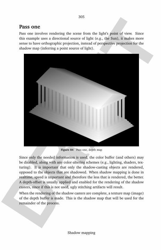
DRAF

T

305

Shadow mapping

Pass onePass one involves rendering the scene from the light’s point of view. Sincethis example uses a directional source of light (e.g., the Sun), it makes moresense to have orthographic projection, instead of perspective projection for theshadow map (inferring a point source of light).

Figure 84 Pass one, depth map

Since only the needed information is used, the color buffer (and others) maybe disabled, along with any color-altering schemes (e.g., lighting, shaders, tex-turing). It is important that only the shadow-casting objects are rendered,opposed to the objects that are shadowed. When shadow mapping is done inrealtime, speed is important and therefore the less that is rendered, the better.A depth-offset is usually applied and enabled for the rendering of the shadowcasters, since if this is not used, ugly stitching artifacts will result.

When the rendering of the shadow casters are complete, a texture map (image)of the depth buffer is made. This is the shadow map that will be used for theremainder of the process.

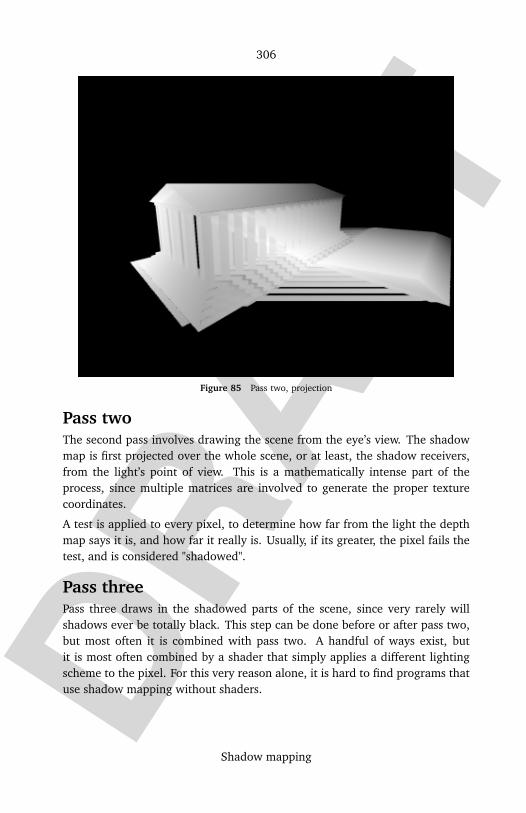
DRAF

T

306

Shadow mapping

Figure 85 Pass two, projection

Pass twoThe second pass involves drawing the scene from the eye’s view. The shadowmap is first projected over the whole scene, or at least, the shadow receivers,from the light’s point of view. This is a mathematically intense part of theprocess, since multiple matrices are involved to generate the proper texturecoordinates.

A test is applied to every pixel, to determine how far from the light the depthmap says it is, and how far it really is. Usually, if its greater, the pixel fails thetest, and is considered "shadowed".

Pass threePass three draws in the shadowed parts of the scene, since very rarely willshadows ever be totally black. This step can be done before or after pass two,but most often it is combined with pass two. A handful of ways exist, butit is most often combined by a shader that simply applies a different lightingscheme to the pixel. For this very reason alone, it is hard to find programs thatuse shadow mapping without shaders.

DRAF

T

307

Shadow mapping

Figure 86 Pass two, failures

Figure 87 Pass two complete

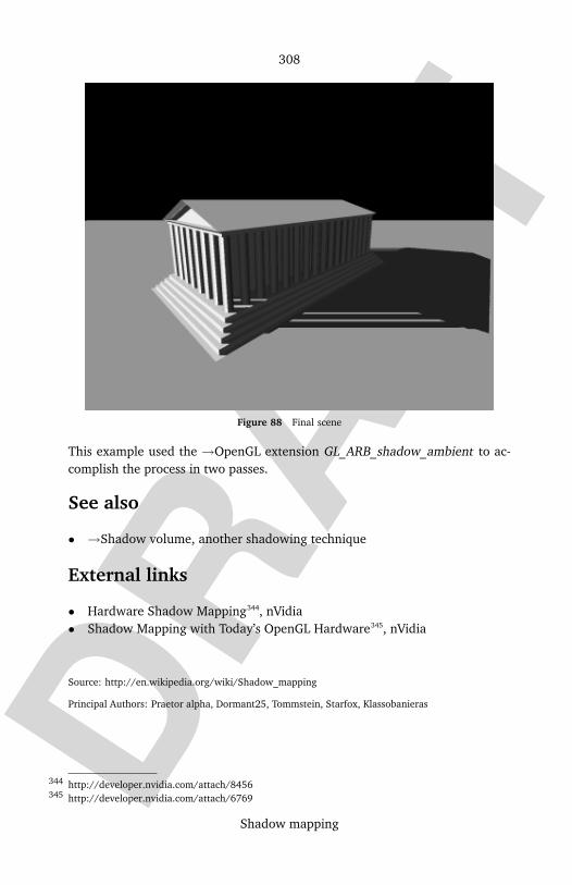
DRAF

T

308

Shadow mapping

Figure 88 Final scene

This example used the →OpenGL extension GL_ARB_shadow_ambient to ac-complish the process in two passes.

See also

• →Shadow volume, another shadowing technique

External links

• Hardware Shadow Mapping344, nVidia• Shadow Mapping with Today’s OpenGL Hardware345, nVidia

Source: http://en.wikipedia.org/wiki/Shadow_mapping

Principal Authors: Praetor alpha, Dormant25, Tommstein, Starfox, Klassobanieras

http://developer.nvidia.com/attach/8456344

http://developer.nvidia.com/attach/6769345

DRAF

T

309

Shadow volume

Shadow volume

Shadow volumes are a technique used in →3D computer graphics since 1977to add shadows to a rendered scene. It is generally considered among the mostpractical general purpose real-time shadowing systems given the capabilitiesof modern 3D graphics hardware, and has been popularized by the computergame Doom 3.

A shadow volume divides the virtual world into two; areas that are in shadowand areas that are not.

ConstructionIn order to construct a shadow volume, project a line from the light througheach vertex in the shadow casting object to some point (generally at infinity).These projections will together form a volume; any point inside that volume isin shadow, everything outside is lit by the light.

Actual shadow volumes are computed in the following way:

• Find all silhouette edges (edges which separate front-facing faces fromback-facing faces)

• Extend all silhouette edges in the direction away from the light-source toform quadrilateral surfaces

• Add front-cap and back-cap to the surfaces to form a closed volume (maynot be necessary, depending on the implementation used)

UsageCurrent research and implementations focus on the use of a hardware stencilbuffer to optimize the algorithm making use of hardware acceleration - see→Stencil shadow volume.

In order to test whether a given pixel in the rendered image is shadowed or not,the shadow volume itself is rendered, though to the stencil buffer only and notto the final image. For every front-facing face in the shadow volume the valuein the stencil buffer is increased; for every back-facing face it is decreased.

Once all faces in the shadow volume have been rendered to the stencil buffer,any pixel with a value not equal to zero will be in shadow.

In order to understand why, think in terms of a ray of light heading back fromthe pixel on the screen - if it passes into the shadow volume, it will be througha front-facing face and so the stencil buffer value will be increased. If it then

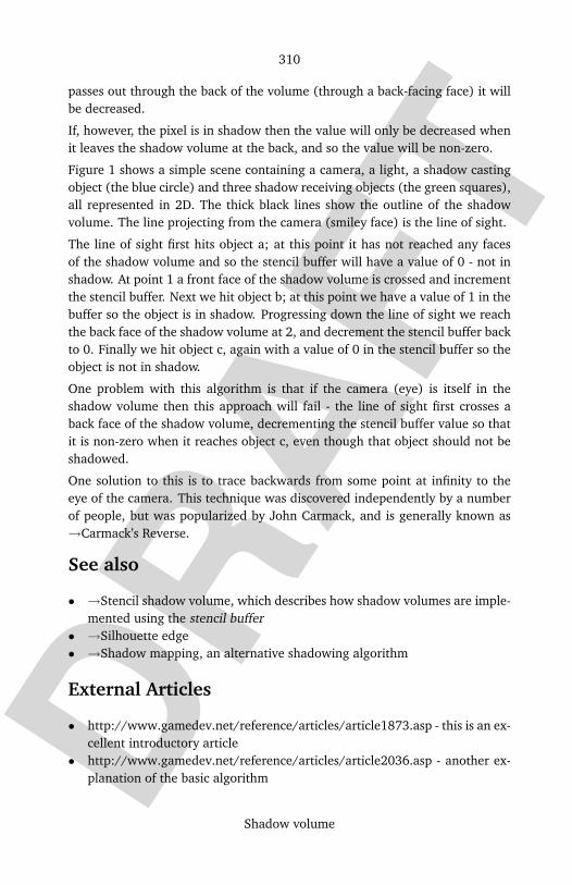
DRAF

T

310

Shadow volume

passes out through the back of the volume (through a back-facing face) it willbe decreased.

If, however, the pixel is in shadow then the value will only be decreased whenit leaves the shadow volume at the back, and so the value will be non-zero.

Figure 1 shows a simple scene containing a camera, a light, a shadow castingobject (the blue circle) and three shadow receiving objects (the green squares),all represented in 2D. The thick black lines show the outline of the shadowvolume. The line projecting from the camera (smiley face) is the line of sight.

The line of sight first hits object a; at this point it has not reached any facesof the shadow volume and so the stencil buffer will have a value of 0 - not inshadow. At point 1 a front face of the shadow volume is crossed and incrementthe stencil buffer. Next we hit object b; at this point we have a value of 1 in thebuffer so the object is in shadow. Progressing down the line of sight we reachthe back face of the shadow volume at 2, and decrement the stencil buffer backto 0. Finally we hit object c, again with a value of 0 in the stencil buffer so theobject is not in shadow.

One problem with this algorithm is that if the camera (eye) is itself in theshadow volume then this approach will fail - the line of sight first crosses aback face of the shadow volume, decrementing the stencil buffer value so thatit is non-zero when it reaches object c, even though that object should not beshadowed.

One solution to this is to trace backwards from some point at infinity to theeye of the camera. This technique was discovered independently by a numberof people, but was popularized by John Carmack, and is generally known as→Carmack’s Reverse.

See also

• →Stencil shadow volume, which describes how shadow volumes are imple-mented using the stencil buffer

• →Silhouette edge• →Shadow mapping, an alternative shadowing algorithm

External Articles

• http://www.gamedev.net/reference/articles/article1873.asp - this is an ex-cellent introductory article

• http://www.gamedev.net/reference/articles/article2036.asp - another ex-planation of the basic algorithm

DRAF

T

311

Silhouette edge

Source: http://en.wikipedia.org/wiki/Shadow_volume

Principal Authors: Orderud, Steve Leach, Staz69uk, Cma, LiDaobing

Silhouette edge

In computer graphics, a silhouette edge on a 3D body projected onto a 2Dplane (display plane) is the collection of points whose outwards surface normalis perpendicular to the view vector. Due to discontinities in the surface normal,a silhouette edge is also an edge which separates a front facing face from aback facing face. Without loss of generality, this edge is usually chosen to bethe closest one on a face, so that in parallel view this edge corresponds to thesame one in a perspective view. Hence, if there is an edge between a frontfacing face and a side facing face, and another edge between a side facing faceand back facing face, the closer one is chosen. The easy example is looking ata cube in the direction where the face normal is colinear with the view vector.

The first type of silhouette edge is sometimes troublesome to handle becauseit does not necessarily correspond to a physical edge in the CAD model. Thereason that this can be an issue is that a programmer might corrupt the originalmodel by introducing the new silhouette edge into the problem. Also, giventhat the edge strongly depends upon the orientation of the model and viewvector, this can introduce numerical instablities into the algorithm (such aswhen a trick like dilution of precision is considered).

ComputationTo determine the silhouette edge of an object, we first have to know the planeequation of all faces. Then, by examining the sign of the point-plane distancefrom the light-source to each face

ax + by + cz + d =

> 0 front facing

= 0 parallel

< 0 back facing

we can determine if the edges is front- or back facing.

The silhouette edge(s) consist of all edges separating a front facing face froma back facing face.

DRAF

T

312

Solid modelling

External links

Source: http://en.wikipedia.org/wiki/Silhouette_edge

Principal Authors: Orderud, Wheger, Gaius Cornelius, David Levy, RJHall

Solid modelling

Solid modelling (or modeling) is the unambiguous representation of the solidparts of an object, that is, models of solid objects suitable for computer process-ing. It is also known as volume modelling. Other modelling methods includesurface models (used extensively in automotive and consumer product designas well as entertainment animation) and wire frame models (which can beambiguous about solid volume).

Primary uses of solid modelling are for CAD, engineering analysis, computergraphics and animation, rapid prototyping, medical testing, product visualiza-tion and visualization of scientific research.

Basic theoretical concepts

• Sweeping• An area feature is "swept out" by moving a primitive along a path to form

a solid feature. These volumes either add to the object ("extrusion") orremove material ("cutter path").

• Also known as ’sketcher based modelling’.• Analogous to various manufacturing techniques such as extrusion,

milling, lathe and others.

• Boundary representation (BREP)• A solid object is represented by boundary surfaces and then filled to

make solid.• Also knowing as ’surfacing’.• Analogous to various manufacturing techniques; Injection moulding,

casting, forging, thermoforming, etc.

• Parameterized primitive instancing.

DRAF

T

313

Solid modelling

• An object is specified by reference to a library of parameterized primi-tives.

• For example, a bolt is modelled for a library, this model is used for allbolt sizes by modifying a set of its parameters.

• Spatial occupancy (voxel)• The whole space is subdivided into regular cells, and the object is spec-

ified by the set of cells it occupies.• Models described this way lend themselves to Finite difference analysis.• This is usually done after a model is made, as part of automated pre-

processing for analysis software.

• Facet modeling• Forming the outside surface form of the volume from any triangular

planes• Often used in reverse engineering of physical models.

• Decomposition• Similar to "spatial occupancy", but the cells are neither regular, nor "pre-

fabricated".• Models described this way lend themselves to FEA.• This is usually done after a model is made, as part of automated pre-

processing for analysis software.

• →Constructive solid geometry• Simple objects are combined using boolean operators such as union,

difference, and intersection.

• Feature based modelling• Complex combinations of objects and operators are considered together

as a unit which can be modified or duplicated.• Order of operations is kept in a history tree, and parametric changes can

propagate through the tree.

• Parametric modelling• Attributes of features are parameterized, giving them labels rather than

only giving them fixed numeric dimensions, and relationships betweenparameters in the entire model are tracked, to make changing numericvalues of parameters easier.

• Almost always combined with features, giving parametric feature basedmodelling.

DRAF

T

314

Solid modelling

HistorySolid modeling has to be seen in context of the whole history of CAD, the keymilestones being the development of Romulus which went on to influence thedevelopment of Parasolid and ACIS and thus the mid-range Windows basedfeature modelers such as SolidWorks and Solid Edge and the arrival of para-metric solid models system like T-Flex and Pro/Engineer.

Practical applications

Parametric Solid modelling CADSolid modellers have become commonplace in engineering departments in thelast ten years due to faster PCs and competitive software pricing. They are theworkhorse of machine designers.

Solid modelling software creates a virtual 3D representation of components formachine design and analysis. Interface with the human operator is highly op-timized and includes programmable macros, keyboard shortcuts and dynamicmodel manipulation. The ability to dynamically re-orient the model, in real-time shaded 3-D, is emphasized and helps the designer maintain a mental 3-Dimage.

Design work on components is usually done within context of the whole prod-uct using assembly modelling methods.

A solid model generally consists of a group of features, added one at a time,until the model is complete. Engineering solid models are built mostly withsketcher-based features; 2-D sketches that are swept along a path to become3-D. These may be cuts, or extrusions for example.

Another type of modelling technique is ’surfacing’ (Freeform surface mod-elling). Here, surfaces are defined, trimmed and merged, and filled to makesolid. The surfaces are usually defined with datum curves in space and a va-riety of complex commands. Surfacing is more difficult, but better applicableto some manufacturing techniques, like injection molding. Solid models for in-jection molded parts usually have both surfacing and sketcher based features.

Engineering drawings are created semi-automatically and reference the solidmodels.

The learning curve for these software packages is steep, but a fluent machinedesigner who can master these software packages is highly productive.

The modelling of solids is only the minimum requirement of a CAD system’scapabilities.

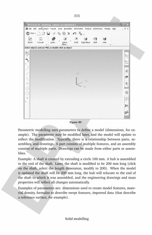
DRAF

T

315

Solid modelling

Figure 89

Parametric modelling uses parameters to define a model (dimensions, for ex-ample). The parameter may be modified later, and the model will update toreflect the modification. Typically, there is a relationship between parts, as-semblies, and drawings. A part consists of multiple features, and an assemblyconsists of multiple parts. Drawings can be made from either parts or assem-blies.

Example: A shaft is created by extruding a circle 100 mm. A hub is assembledto the end of the shaft. Later, the shaft is modified to be 200 mm long (clickon the shaft, select the length dimension, modify to 200). When the modelis updated the shaft will be 200 mm long, the hub will relocate to the end ofthe shaft to which it was assembled, and the engineering drawings and massproperties will reflect all changes automatically.

Examples of parameters are: dimensions used to create model features, mate-rial density, formulas to describe swept features, imported data (that describea reference surface, for example).

DRAF

T

316

Solid modelling

Related to parameters, but slightly different are Constraints. Constraints arerelationships between entities that make up a particular shape. For a window,the sides might be defined as being parallel, and of the same length.

Parametric modelling is obvious and intuitive. But for the first three decadesof CAD this was not the case. Modification meant re-draw, or add a new cutor protrusion on top of old ones. Dimensions on engineering drawings werecreated, instead of shown.

Parametric modelling is very powerful, but requires more skill in model cre-ation. A complicated model for an injection molded part may have a thousandfeatures, and modifying an early feature may cause later features to fail. Skill-fully created parametric models are easier to maintain and modify.

Parametric modelling also lends itself to data re-use. A whole family of cap-screws can be contained in one model, for example.

EntertainmentAnimation of a computer generated character is an example of parametricmodelling. Jar Jar Binks is described by parameters which locate key bodypositions. The model is then built off these locations. The parameters aremodified, and the model rebuilt, for each frame to create animation.

Medical solid modellingModern computed axial tomography and magnetic resonance imaging scannerscan construct solid models of interior body features.

Uses of medical solid modelling;

• Visualization• Visualization of specific body tissues (just blood vessels and tumor, for ex-

ample)• Creating solid model data for rapid prototyping (to aid surgeons preparing

for difficult surgeries, for example)• Combining medical solid models with CAD solid modelling (design of hip

replacement parts, for example)

See also

• Computer graphics• Computational geometry• Euler boundary representation• Engineering drawing

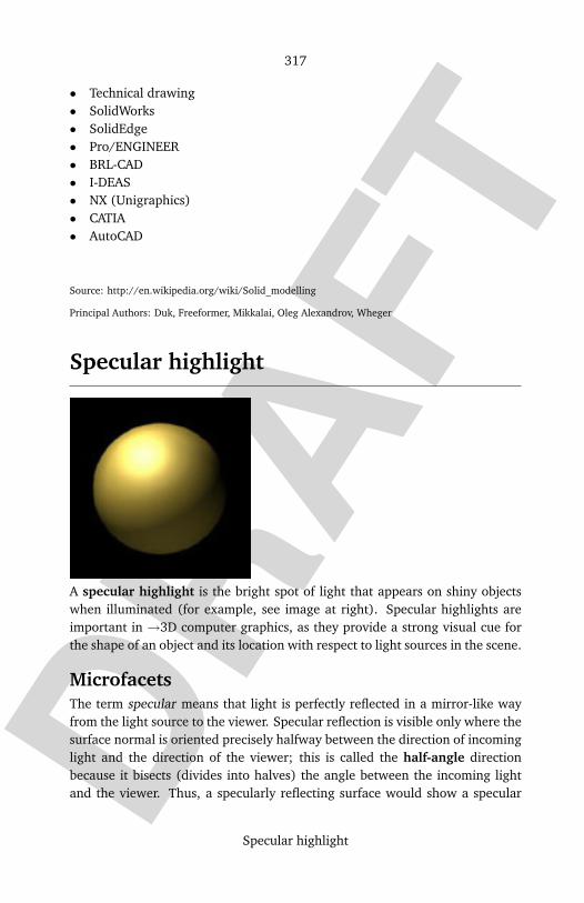
DRAF

T

317

Specular highlight

• Technical drawing• SolidWorks• SolidEdge• Pro/ENGINEER• BRL-CAD• I-DEAS• NX (Unigraphics)• CATIA• AutoCAD

Source: http://en.wikipedia.org/wiki/Solid_modelling

Principal Authors: Duk, Freeformer, Mikkalai, Oleg Alexandrov, Wheger

Specular highlight

A specular highlight is the bright spot of light that appears on shiny objectswhen illuminated (for example, see image at right). Specular highlights areimportant in →3D computer graphics, as they provide a strong visual cue forthe shape of an object and its location with respect to light sources in the scene.

MicrofacetsThe term specular means that light is perfectly reflected in a mirror-like wayfrom the light source to the viewer. Specular reflection is visible only where thesurface normal is oriented precisely halfway between the direction of incominglight and the direction of the viewer; this is called the half-angle directionbecause it bisects (divides into halves) the angle between the incoming lightand the viewer. Thus, a specularly reflecting surface would show a specular

DRAF

T

318

Specular highlight

highlight as the perfectly sharp reflected image of a light source. However,many shiny objects show blurred specular highlights.

This can be explained by the existence of microfacets. We assume that surfacesthat are not perfectly smooth are composed of many very tiny facets, eachof which is a perfect specular reflector. These microfacets have normals thatare distributed about the normal of the approximating smooth surface. Thedegree to which microfacet normals differ from the smooth surface normal isdetermined by the roughness of the surface.

The reason for blurred specular highlights is now clear. At points on the ob-ject where the smooth normal is close to the half-angle direction, many of themicrofacets point in the half-angle direction and so the specular highlight isbright. As one moves away from the center of the highlight, the smooth nor-mal and the half-angle direction get farther apart; the number of microfacetsoriented in the half-angle direction falls, and so the intensity of the highlightfalls off to zero.

The specular highlight often reflects the color of the light source, not the colorof the reflecting object. This is because many materials have a thin layer ofclear material above the surface of the pigmented material. For example plas-tic is made up of tiny beads of color suspended in a clear polymer and humanskin often has a thin layer of oil or sweat above the pigmented cells. Such ma-terials will show specular highlights in which all parts of the color spectrum arereflected equally. On metallic materials such as gold the color of the specularhighlight will reflect the color of the material.

Models of MicrofacetsA number of different models exist to predict the distribution of microfacets.Most assume that the microfacet normals are distributed evenly around thenormal; these models are called isotropic. If microfacets are distributedwith a preference for a certain direction along the surface, the distributionis anisotropic.

Phong distributionIn the →Phong reflection model, the intensity of the specular highlight is calcu-lated as kspec = cosn(R, V ), where R is the mirror reflection of the light vectoroff the surface, and V is the viewpoint vector.

In Blinn-Phong shading, the intensity of a specular highlight is calculated askspec = cosn(N,H), where N is the smooth surface normal and H is the half-angle direction (the direction vector midway between L, the vector to the light,and V, the viewpoint vector).

DRAF

T

319

Specular highlight

The number n is called the Phong exponent, and is a user-chosen value thatcontrols the apparent smoothness of the surface. These equations imply thatthe distribution of microfacet normals is an approximately Gaussian distri-bution, or approximately Pearson type II distribution, of the correspondingangle.346 While this is a useful heuristic and produces believable results, it isnot a physically based model.

Gaussian distributionA slightly better model of microfacet distribution can be created using a Gaus-sian distribution. The usual function calculates specular highlight intensity as:

kspec = e−(

∠(N,H)m

)2

where m is a constant between 0 and 1 that controls the apparent smoothnessof the surface.

Material from this section adapted from: Glassner, Andrew S. (ed). AnIntroduction to Ray Tracing. San Diego: Academic Press Ltd, 1989. p. 148.

Beckmann distributionA physically based model of microfacet distribution is the Beckmann distribu-tion. This function gives very accurate results, but is also rather expensive tocompute.

kspec = 14m2 cos4(N,H)e

−(

tan(N,H)m

)2

where m is as before: a constant between 0 and 1 that controls the apparentsmoothness of the surface.

Material from this section adapted from: Foley et al. Computer Graphics:Principles and Practice. Menlo Park: Addison-Wesley, 1990. p. 764.

Heidrich-Seidel anisotropic distributionThe Heidrich-Seidel distribution is a simple anisotropic distribution, based onthe Phong model. It can be used to model surfaces that have small parallelgrooves or fibers, such as brushed metal, satin, and hair. The specular highlightintensity for this distribution is:

Richard Lyon, "Phong Shading Reformulation for Hardware Renderer Simplification", Apple Technical346

Report #43, Apple Computer, Inc. 1993

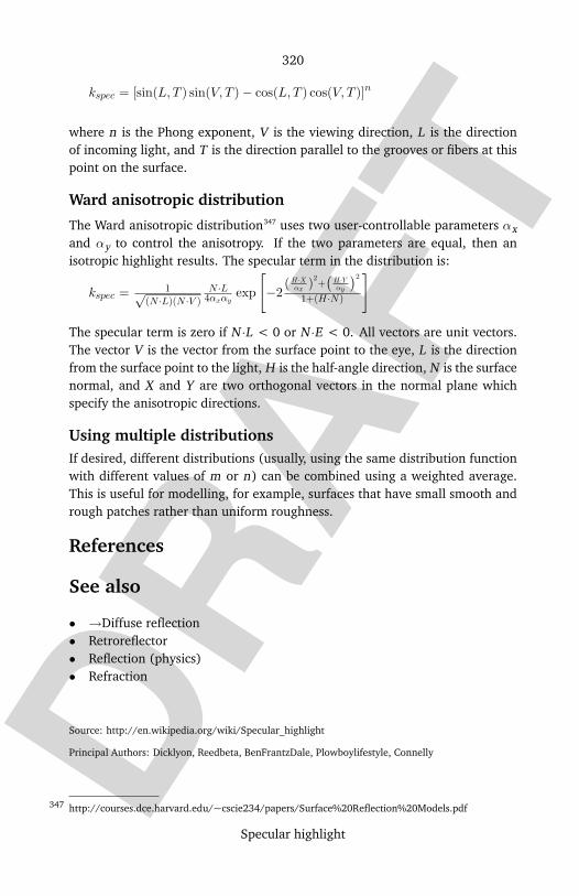
DRAF

T

320

Specular highlight

kspec = [sin(L, T ) sin(V, T )− cos(L, T ) cos(V, T )]n

where n is the Phong exponent, V is the viewing direction, L is the directionof incoming light, and T is the direction parallel to the grooves or fibers at thispoint on the surface.

Ward anisotropic distribution

The Ward anisotropic distribution347 uses two user-controllable parameters αxand αy to control the anisotropy. If the two parameters are equal, then anisotropic highlight results. The specular term in the distribution is:

kspec = 1√(N ·L)(N ·V )

N ·L4αxαy exp

[−2

(H·Xαx )2+(H·Yαy

)2

1+(H·N)

]

The specular term is zero if N ·L < 0 or N ·E < 0. All vectors are unit vectors.The vector V is the vector from the surface point to the eye, L is the directionfrom the surface point to the light, H is the half-angle direction, N is the surfacenormal, and X and Y are two orthogonal vectors in the normal plane whichspecify the anisotropic directions.

Using multiple distributionsIf desired, different distributions (usually, using the same distribution functionwith different values of m or n) can be combined using a weighted average.This is useful for modelling, for example, surfaces that have small smooth andrough patches rather than uniform roughness.

References

See also

• →Diffuse reflection• Retroreflector• Reflection (physics)• Refraction

Source: http://en.wikipedia.org/wiki/Specular_highlight

Principal Authors: Dicklyon, Reedbeta, BenFrantzDale, Plowboylifestyle, Connelly

http://courses.dce.harvard.edu/~cscie234/papers/Surface%20Reflection%20Models.pdf347

DRAF

T

321

Stencil buffer

Specularity

Specularity is the quality used in many 3D rendering programs to set the sizeand the brightness of a texture’s reflection to light.

Adding specularity into a render allows one to add highlights to an object.

Specularity only provides an illusion of reflection to the light. The function ofspecularity only provides a central hotspot and the halo surrounding it.

In some situations, specularity is preferred over reflection because of fasterrender speeds (due to the complexity of raytracing in reflection algorithms)and because, even though reflection mapping is more realistic, specularity al-gorithms often appear more realistic.

External links

• Leigh Van Der Byl Specularity Tutorial348

Source: http://en.wikipedia.org/wiki/Specularity

Principal Authors: Neonstarlight, Frap, Volfy, Megan1967, Oliver Lineham

Stencil buffer

A stencil buffer is an extra buffer, in addition to the color buffer (pixel buffer)and depth buffer (z-buffer) found on modern computer graphics hardware.The buffer is per pixel, and works on integer values, usually with a depth ofone byte per pixel. The depth buffer and stencil buffer often share the samearea in the RAM of the graphics hardware.

In the simplest case, the stencil buffer is used to limit the area of rendering(stenciling). More advanced usage of the stencil buffer make use of the strongconnection between the depth buffer and the stencil buffer in the renderingpipeline (for example, stencil values can be automatically increased/decreasedfor every pixel that failed or passed the depth test).

The simple combination of depth test and stencil modifiers make a vast num-ber of effects possible (such as shadows, outline drawing or highlighting of

http://leigh.cgcommunity.com/tutorialspart5.htm348

DRAF

T

322

Stencil shadow volume

intersections between complex primitives) though they often require severalrendering passes and, therefore, can put a heavy load on the graphics hard-ware.

The most typical application is still to add shadows to 3D applications.

The stencil buffer and its modifiers can be accessed in computer graphics APIslike →OpenGL and →Direct3D.

See also

• →Z-buffering (depth buffer)• →Stencil shadow volume

Source: http://en.wikipedia.org/wiki/Stencil_buffer

Principal Authors: Cyc, Claynoik, Eep2, Orderud, Ddawson


A stencil shadow volume is a method of rendering in→3D computer graphics.Frank Crow introduced shadow volumes in 1977 as the geometry describingthe 3D shape of the region occluded from a light source. Tim Heidmann latershowed how to use the stencil buffer to render shadows with shadow volumesin real time. Heidmann’s approach only worked when the virtual camera wasitself not in shadow. Around 2000, several people discovered that Heidmann’smethod can be made to work for all camera positions by reversing a test basedon the z-coordinate. His original method is now known as z-pass and the newmethod is called z-fail. Sim Dietrich’s PowerPoint talk at a Creative Labs talkappears to be the first to mention this; however, Cass Everitt and Mark Kilgard’s2002 NVIDIA technical report is the first detailed analysis of the technique.John Carmack of id Software popularized the technique by using it in the Doom3 video game, so it is often referred to as →Carmack’s Reverse.

Creative Labs has recently attempted to enforce a patent on z-fail testing.

DRAF

T

323


VariantsThere are several ways of implementing stencil shadow volumes, all of whichuse the stencil buffer available in both →OpenGL and DirectX. The variantsdiffer in speed, robustness and the number of stencil-bits required.

All variants require the construction of a shadow volume first, using the prop-erties of silhouette edges.

Exclusive-Or variantThis is the fastest and simplest variant, requiring only a single additional pass.This method also only requires a single bit in the stencil buffer.

1. Render scene with only ambient lighting2. Render entire shadow volume to the stencil buffer. Invert stencil value on

z-pass3. Render scene with diffuse and specular lighting in areas of zero stencil value

This variant has the drawback of intersecting shadow volumes canceling outeach other. It also fails if the camera is inside a shadow volume.

Depth-pass variantThis is a more advanced stencil counting approach capable of handling inter-secting shadow volumes.

1. Render scene with only ambient lighting2. Render front-facing faces to the stencil buffer. Increment stencil value on

z-pass3. Render back-facing faces to the stencil buffer. Decrement stencil value on

z-pass4. Render scene with diffuse and specular lighting in areas of zero stencil value

The near-plane is a plane in front of the camera; it is used to clip geometry thatis in front of that plane. The Depth-pass variant of the stencil shadow volumealgorithm fails if the near-rectangle (the portion of the near-plane visible bythe camera) intersects a shadow volume. It is possible, however, to ’repair’such failure, with an additional rendering pass, see ZP+ in the External linkssection, below.

Depth-fail variant (Carmack’s Reverse)This is an even more advanced stencil counting approach capable of handlingboth intersecting shadow volumes and cameras inside the shadow volumes.

DRAF

T

324


1. Render scene with only ambient lighting2. Render back-facing faces to the stencil buffer. Increment stencil value on

z-fail3. Render front-facing faces to the stencil buffer. Decrement stencil value on

z-fail4. Render scene with diffuse and specular lighting in areas of zero stencil value

This variant does not fail if the camera is inside a shadow volume, but requiresclosed shadow volumes which can be expensive to compute.

Common problems

• Non-convex objects may have self-intersecting silhouettes, leading to ar-tifacts in the shadows if this is not accounted for (by removing all self-intersections before rendering).

• Stencil buffer uses saturation arithmetic, which may lead to problems if theinitial stencil value is zero.

See also

• →Shadow volume, which describes the general algorithm• →Silhouette edge, used to determine the shadow volume• →Stencil buffer, the buffer used

External links

• The Theory of Stencil Shadow Volumes349 by Hun Yen Kwoon onGameDev.net

• Tutorial - Stenciled Shadow Volumes in OpenGL350 by Josh Beam on3ddrome

• ZP+: correct Z-pass stencil shadows351

Source: http://en.wikipedia.org/wiki/Stencil_shadow_volume

Principal Authors: Orderud, Staz69uk, Gracefool, HopeSeekr of xMule, Boredzo


http://www.3ddrome.com/articles/shadowvolumes.php350

http://artis.inrialpes.fr/Publications/2005/HHLH05/351

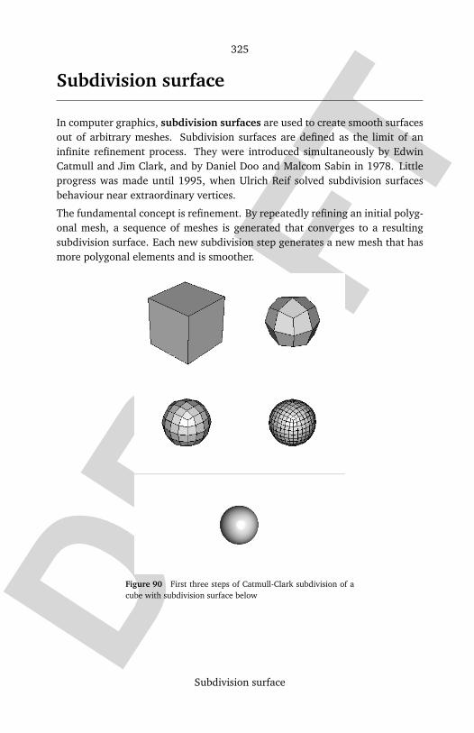
DRAF

T

325

Subdivision surface

Subdivision surface

In computer graphics, subdivision surfaces are used to create smooth surfacesout of arbitrary meshes. Subdivision surfaces are defined as the limit of aninfinite refinement process. They were introduced simultaneously by EdwinCatmull and Jim Clark, and by Daniel Doo and Malcom Sabin in 1978. Littleprogress was made until 1995, when Ulrich Reif solved subdivision surfacesbehaviour near extraordinary vertices.

The fundamental concept is refinement. By repeatedly refining an initial polyg-onal mesh, a sequence of meshes is generated that converges to a resultingsubdivision surface. Each new subdivision step generates a new mesh that hasmore polygonal elements and is smoother.

Figure 90 First three steps of Catmull-Clark subdivision of acube with subdivision surface below

DRAF

T

326

Subdivision surface

Subdivision methodsThere are several refinement schemes:

• Catmull-Clark is a generalization of bi-cubic uniform B-splines• Doo-Sabin is a generalization of bi-quadratic uniform B-splines• Loop, by Charles Loop, is a generalization of quartic triangular box splines

(works with triangular meshes)• Butterfly named after the scheme’s shape• Midedge• Kobbelt is a variational subdivision method that tries to overcome uniform

subdivision drawbacks

Advantages over NURBS modellingSubdivision surface modeling is now preferred over NURBS modeling in majormodelers because subdivision surfaces have many benefits:

• work with more complex topology• numerically stable• easier to implement• local continuity control• local refinement• no tesselation issue• switch between coarser and finer refinement

B-spline relationshipB-spline curves are refinable: their control point sequence can be refined andthe iteration process converges to the actual curve. This is a useless propertyfor curves, but its generalization to surfaces yields subdivision surfaces.

Refinement processInterpolation inserts new points while original ones remain undisturbed.

Refinement inserts new points and moves old ones in each step of subdivision.

Extraordinary pointsThe Catmull-Clark refinement scheme is a generalization of bi-cubic uniformB-splines. Any portion of the surface that is equivalent to a 4x4 grid of controlpoints represents a bi-cubic uniform B-spline patch. Surface refinement is easyin those areas where control points valence is equal to four. Defining a subdi-vision surface at vertices with valence other than four was historically difficult;

DRAF

T

327

Subsurface scattering

such points are called extraordinary points. Similarly, extraordinary points inthe Doo-Sabin scheme have a valence other than three.

Most schemes don’t produce extraordinary vertices during subdivision.

External links

• Resources about subdvisions352

• Geri’s Game353 : Oscar winning animation by Pixar completed in 1997 thatintroduced subdivision surfaces (along with cloth simulation)

• Subdivision for Modeling and Animation354 tutorial, SIGGRAPH 2000course notes

• A unified approach to subdivision algorithms near extraordinary vertices355,Ulrich Reif (Computer Aided Geometric Design 12(2):153-174 March1995)

Source: http://en.wikipedia.org/wiki/Subdivision_surface

Principal Authors: Orderud, Romainbehar, Furrykef, Lauciusa, Feureau


Subsurface scattering (or SSS) is a mechanism of light transport in whichlight penetrates the surface of a translucent object, is scattered by interactingwith the material, and exits the surface at a different point. The light willgenerally penetrate the surface and be reflected a number of times at irregularangles inside the material, before passing back out of the material at an angleother than the angle it would reflect at had it reflected directly off the surface.Subsurface scattering is important in →3D computer graphics, being necessaryfor the realistic rendering of materials such as marble, skin, and milk.

http://www.subdivision.org/subdivision/index.jsp352

http://www.pixar.com/shorts/gg/theater/index.html353

http://www.mrl.nyu.edu/dzorin/sig00course/354

http://dx.doi.org/10.1016/0167-8396(94)00007-F355

DRAF

T

328


Figure 91 Three dimensional object with subsurface scattering

External links

• Henrik Wann Jensen’s subsurface scattering website356

• An academic paper by Jensen on modelling subsurface scattering357

• Simple superficial surface scattering for Blender358

Source: http://en.wikipedia.org/wiki/Subsurface_scattering

Principal Authors: Reedbeta, T-tus, Rufous, RJHall, ALoopingIcon

http://graphics.ucsd.edu/~henrik/images/subsurf.html356

http://graphics.ucsd.edu/~henrik/papers/bssrdf/357

http://www.dedalo-3d.com/index.php?filename=SXCOL/mh_ssss/abstract.html358

DRAF

T

329

Surface normal

Surface caching

Surface caching is a computer graphics technique pioneered by John Carma-ck, first used in the computer game Quake. The traditional method of lightinga surface is to calculate the surface from the perspective of the viewer, and thenapply the lighting to the surface. Carmack’s technique is to light the surface in-dependent of the viewer, and store that surface in a cache. The lighted surfacecan then be used in the normal rendering pipeline for any number of frames.

Surface caching is one of the reasons that it became practical to make a true3D game that was reasonably fast on a 66 MHz Pentium microprocessor.

External links

• Quake’s Lighting Model: Surface Caching359 - an in-depth explanation byMichael Abrash

Source: http://en.wikipedia.org/wiki/Surface_caching

Principal Authors: Fredrik, KirbyMeister, Schneelocke, Tregoweth, Hephaestos

Surface normal

A surface normal, or just normal to a flat surface is a three-dimensional vectorwhich is perpendicular to that surface. A normal to a non-flat surface at a pointp on the surface is a vector which is perpendicular to the tangent plane to thatsurface at p. The word normal is also used as an adjective as well as a nounwith this meaning: a line normal to a plane, the normal component of a force,the normal vector, etc.

Calculating a surface normalFor a polygon (such as a triangle), a surface normal can be calculated as thevector cross product of two edges of the polygon.

For a plane given by the equation ax + by + cz = d, the vector (a, b, c) is anormal.

http://www.bluesnews.com/abrash/chap68.shtml359

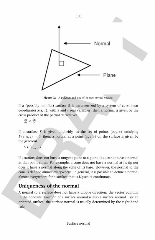
DRAF

T

330

Surface normal

Figure 92 A polygon and one of its two normal vectors.

If a (possibly non-flat) surface S is parametrized by a system of curvilinearcoordinates x(s, t), with s and t real variables, then a normal is given by thecross product of the partial derivatives

∂x∂s ×

∂x∂t .

If a surface S is given implicitly, as the set of points (x, y, z) satisfyingF (x, y, z) = 0, then, a normal at a point (x, y, z) on the surface is given bythe gradient

∇F (x, y, z).

If a surface does not have a tangent plane at a point, it does not have a normalat that point either. For example, a cone does not have a normal at its tip nordoes it have a normal along the edge of its base. However, the normal to thecone is defined almost everywhere. In general, it is possible to define a normalalmost everywhere for a surface that is Lipschitz continuous.

Uniqueness of the normalA normal to a surface does not have a unique direction; the vector pointingin the opposite direction of a surface normal is also a surface normal. For anoriented surface, the surface normal is usually determined by the right-handrule.

DRAF

T

331

Synthespian

Uses

• Surface normals are essential in defining surface integrals of vector fields.• Surface normals are commonly used in →3D computer graphics for lighting

calculations; see →Lambert’s cosine law.

External link

• An explanation of normal vectors360 from Microsoft’s MSDN

Source: http://en.wikipedia.org/wiki/Surface_normal

Principal Authors: Oleg Alexandrov, Frecklefoot, Olegalexandrov, Patrick, Subhash15

Synthespian

For the Doctor Who novel, see SynthespiansTM.

A synthespian is any synthetic actor. A portmanteau of the words synthetic,meaning not of natural origin, and thespian, meaning dramatic actor. Thedinosaurs in Jurassic Park, for instance, were animatronic synthespians createdby Stan Winston Studios. Aki Ross from the movie Final Fantasy: The SpiritsWithin was an entirely computer-generated synthespian.

The term "synthespian" was created by Jeff Kleiser and Diana Walczak ofKleiser-Walczak Construction Company.361 When they were assembling a syn-thetic thespian for their project, "Nestor Sextone for President", they coined theterm "synthespian".

Source: http://en.wikipedia.org/wiki/Synthespian

Principal Authors: RoyBoy, Pegship, Drat, Sean Black, Khaosworks

http://msdn.microsoft.com/library/default.asp?url=/library/en-us/directx9_c/directx/graphics/pro-360

grammingguide/GettingStarted/3DCoordinateSystems/facevertexnormalvectors.asphttp://www.kwcc.com/works/sp/lead.html361

DRAF

T

332

Texel (graphics)

Tao (software)

For "The ACE ORB", see TAO (software).

The Tao Framework is a library giving .NET and mono developers access topopular graphics and gaming libraries like →OpenGL and SDL.

External links

• Tao homepage362

• Tao wiki363

Source: http://en.wikipedia.org/wiki/Tao_%28software%29

Principal Authors: Orderud, Suruena, Asparagus, Zondor

Texel (graphics)

A texel, or texture element (also texture pixel) is the fundamental unit oftexture space364, used in computer graphics. Textures are represented by arraysof texels, just as pictures are represented by arrays of pixels.

When texturing a 3D surface, a process known as texture mapping maps tex-els to appropriate pixels in the output picture. On modern computers, thisoperation is accomplished on the graphics card.

References

Source: http://en.wikipedia.org/wiki/Texel_%28graphics%29

Principal Authors: Neckelmann, Nlu, Dicklyon, Neg, ONjA

http://www.mono-project.com/Tao362

http://www.taoframework.com/Home363

Andrew Glassner, An Introduction to Ray Tracing, San Francisco: Morgan–Kaufmann, 1989364

DRAF

T

333

Texture filtering

Texture filtering

In computer graphics, texture filtering is the method used to map texels (pixelsof a texture) to points on a 3D object. There are many methods of texturefiltering, and developers must make a tradeoff between rendering speed andimage quality when choosing a texture filtering algorithm.

The purpose of texture filtering is to accurately represent a texture that isnot aligned to screen coordinates. This is a common problem in 3D graph-ics where textures are wrapped on polygons whose surface is not orthogonalto the screen.

Different methodsThe fastest method is to take a point on an object and look up the closest texelto that position. The resulting point then gets its color from that one texel.This is sometimes referred to as nearest neighbor filtering. It works quite well,but can result in visual artifacts when objects are small, large, or viewed fromodd angles.

Antialiasing means thinking of the pixel and texel as blocks on a grid thattogether make up an image and using the area a texel covers on a pixel as aweight. As this is computionally expensive, a lot of approximations have beeninvented: mip-mapping, supersampling, anisotropic filtering.

Mip-mapping stores multiple copies of a texture at smaller resolutions. Eachmip map is a quarter the resolution of the previous mip map. This speeds uptexture mapping on small polygons.

In bilinear filtering, the four closest texels to the screen coordinate are sampledand the weighted average is used as the final colour. In trilinear filtering,bilinear filtering is done for the nearest two mip map levels and the resultsfrom both mip maps are averaged. This removes mip map transition lines fromthe rendered image.

Both bilinear and trilinear filtering do not take into account the angle at whichthe texture is oriented toward the screen. This produces blurry results fortextures that are at receding angle to the screen.

Anisotropic filtering takes up to 16 samples based on the angle of the texturedpolygon. More texels are sampled at the receding end than the near end. Thisproduces accurate results no matter which way the texture is oriented towardthe screen.

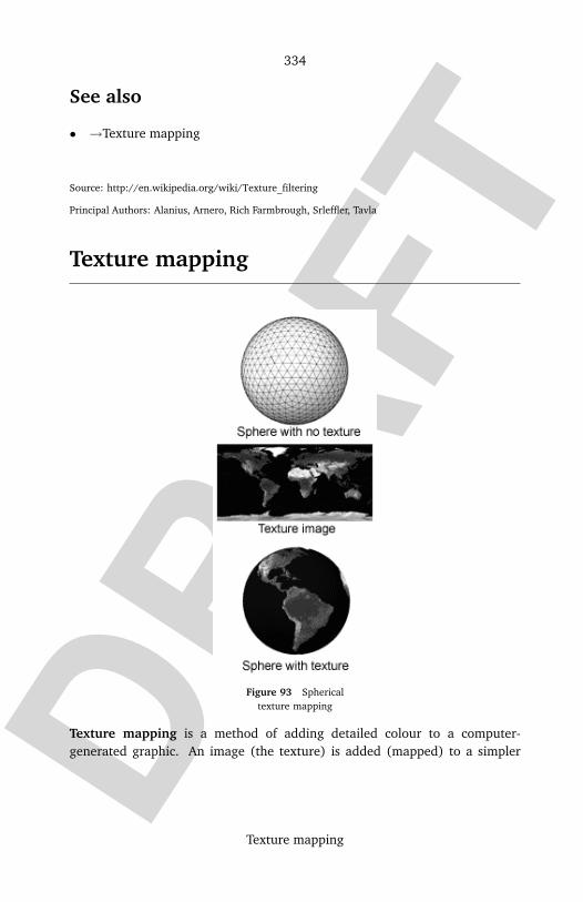
DRAF

T

334

Texture mapping

See also

• →Texture mapping

Source: http://en.wikipedia.org/wiki/Texture_filtering

Principal Authors: Alanius, Arnero, Rich Farmbrough, Srleffler, Tavla

Texture mapping

Figure 93 Sphericaltexture mapping

Texture mapping is a method of adding detailed colour to a computer-generated graphic. An image (the texture) is added (mapped) to a simpler

DRAF

T

335

Texture mapping

shape that is generated in the scene, like a decal pasted onto its surface. This al-lows a complicated colouring of the surface without requiring additional poly-gons to represent minute details.

Multitexturing is the use of more than one texture at a time on a shape. Thishas various uses, sometimes as a way of applying a light map to a surface,which is faster than requiring the graphics hardware to do lighting calculationfor that surface on the fly, or more recently bump mapping has become popular,which allows a texture to directly control the lighting calculations, allowingthe surface to not only have detailed colouring, but detailed contours as well(bumps).

The way the resulting pixels on the screen are calculated from the texels (tex-ture pixels) is governed by texture filtering. The fastest method is to use thenearest neighbour interpolation, but bilinear interpolation is commonly chosenas good tradeoff between speed and accuracy.

At the hardware level usually texture coordinates are specified at each vertexof a given triangle (any polygon may be broken down into triangles for ren-dering), and these coordinates are interpolated as part of a calculation that isan extension of Bresenham’s line algorithm. Direct interpolation of the texturecoordinates between vertices results in affine texture mapping, which causesa percievable discontinuity between adjacent triangles when the 3D geometryof the specified triangle is at an angle to the plane of the screen, perspectivecorrection is thus preferred where realism is important, and adjusts the texturecoordinate interpolation as a function of the 3D depth of each pixel. Becauseperspective correction involves more calculation, it did not become common-place in graphics hardware until recently.

See also

• Edwin Catmull• →Texture filtering• Texture Splatting - a techique for combining textures.

External links

• Graphics for the Masses by Paul Rademacher365

• High resolution textures resource366

http://www.cs.unc.edu/~rademach/xroads-RT/RTarticle.html365

http://www.mayang.com/textures/366

DRAF

T

336

Unified lighting and shadowing

• High resolution images and textures resource367

• Texture Hound | Ultimate 3d Texture Links Directory368

Source: http://en.wikipedia.org/wiki/Texture_mapping

Principal Authors: Arnero, Al Fecund, T-tus, Canadacow, RJHall, AzaToth, Collabi, Viznut

Transform and lighting

Transform and lighting is a term used in computer graphics, generally usedin the context of hardware acceleration (Hardware T&L). Transform refers tothe task of converting spatial coordinates, which in this case involves movingthree-dimensional objects in a virtual world and converting the coordinates toa two-dimensional view. Lighting refers to the task of taking light objects in avirtual scene, and calculating the resulting colour of surrounding objects as thelight falls upon them.

In modern 3D games with complex scenes and detailed lighting effects, thehigh number of points to be transformed and lit is a computationally intenseprocess, which is why 3D graphics cards offer acceleration.

Source: http://en.wikipedia.org/wiki/Transform_and_lighting

Principal Authors: Mel Etitis, GregorB, Gracefool, Peterhuh, Gothmog.es


Unified lighting and shadowing is a lighting model used in the Doom 3 gameengine developed by Id Software.

Previous 3D games like Quake III used separate lighting models for determin-ing how a light would illuminate a character or a map. Lighting and shadow in-formation for maps would be static, pre-generated and stored, whereas lightingand shadowing information for characters would be determined at run-time.

http://www.imageafter.com/367

http://www.texturehound.com/368

DRAF

T

337


Figure 94 Doom 3 uses unified lighting and shadowing. Shadows are calculated using a stencilshadow volume.

Doom 3 claims to use a unified model, which renders every triangle using thesame lighting mechanism, regardless as to whether it originated from a model,or map geometry. This is not strictly true as some models are marked with a’don’t self shadow’ flag, custom material shaders can allow different lightingmechanisms to be employed on different surfaces (most often a reflective cubemap effect), and the point sprite effects (such as explosions) are totally unlit.A renderer using a truly unified lighting system would use an identical set oflighting calculations for every pixel on the screen and would not make suchdistinctions, although Doom 3’s lighting is certainly far ’more unified’ thanprevious games, there is still much more which can be done on recent andfuture hardware to improve the consistency of lighting in games.

Doom 3 does not use →OpenGL’s built in system, instead, it uses its own sys-tem which gives better quality and more accurate illumination than OpenGL’sdefault lighting model.

See also

• →Shadow mapping - a technique for rendering shadows• →Stencil shadow volumes - an alternative method, used for shadows in

Doom 3

DRAF

T

338

Utah teapot

Figure 95 Quake III used an older lighting model in which shadows are calculated differently formoving characters and backgrounds.

Source: http://en.wikipedia.org/wiki/Unified_lighting_and_shadowing

Principal Authors: AlistairMcMillan, Orderud, Jheriko, Michael Hardy, Gracefool

Utah teapot

The Utah teapot or Newell teapot is a 3D model which has become a stan-dard reference object (and something of an in-joke) in the computer graphicscommunity. It is a simple, round, solid, partially concave mathematical modelof an ordinary teapot.

The teapot model was created in 1975 by early computer graphics researcherMartin Newell, a member of the pioneering graphics program at the Universityof Utah.

DRAF

T

339

Utah teapot

Figure 96 The Utah teapot

HistoryNewell needed a moderately simple mathematical model of a familiar objectfor his work. Sandra Newell (his wife) suggested modelling their tea servicesince they were sitting down to tea at the time. He got some graph paper anda pencil, and sketched the entire tea service by eye. Then, he went back tothe lab and edited Bezier control points on a Tektronix storage tube, again byhand. While a cup, saucer, and teaspoon were digitized along with the famousteapot, only the teapot itself attained widespread usage. It is thought that amilk jug was also modelled - but the data for that seems to have been lost.

The teapot shape contains a number of elements that made it ideal for thegraphics experiments of the time — it is round, contains saddle points, has agenus greater than zero because of the hole in the handle, can project a shad-ow on itself, and looks reasonable when displayed without a complex surfacetexture.

Newell made the mathematical data that describes the teapot’s geometry (aset of three-dimensional coordinates) publicly available, and soon other re-searchers began to use the same data for their computer graphics experiments.These researchers needed something with roughly the same characteristics that

DRAF

T

340

Utah teapot

Figure 97 The Melitta teapot that was the prototype for the Utah teapot model.

Newell had, and using the teapot data meant they didn’t have to laboriouslyenter geometric data for some other object. Although technical progress hasmeant that the act of rendering the teapot is no longer the challenge it wasin 1975, the teapot continued to be used as a reference object for increasinglyadvanced graphics techniques.

Over the following decades, editions of computer graphics journals (such as theACM SIGGRAPH’s quarterly) regularly featured versions of the teapot: facetedor smooth-shaded, wireframe, bumpy, translucent, refractive, even leopard-skin and furry teapots were created.

The original teapot model was never intended to be seen from below and hadno surface to represent the base of the teapot; later versions of the data sethave fixed this.

The real teapot is noticeably taller than the computer model because Newell’sframe buffer used non-square pixels. Rather than distorting the image,Newell’s colleague Jim Blinn reportedly scaled the geometry to cancel out thestretching, and when the model was shared with users of other systems, thescaling stuck. Height scale factor was 1.3.

The original, physical teapot was purchased from ZCMI (a department store inSalt Lake City, Utah) in 1974. It was donated to the Boston Computer Museumin 1984 where it was on display until 1990. It now resides in the ephemera col-lection at the Computer History Museum in Mountain View, California where it

DRAF

T

341

Utah teapot

is catalogued as "Teapot used for Computer Graphics rendering" and bears thecatalogue number X00398.1984.

ApplicationsVersions of the teapot model, or sample scenes containing it, are distribut-ed with or freely available for nearly every current rendering and modelingprogram, including AutoCAD, POV-Ray, →OpenGL, →Direct3D, and 3D Stu-dio Max. Along with the expected cubes and spheres, the GLUT library evenprovides the function glutSolidTeapot() as a graphics primitive, as does its→Direct3D counterpart D3DX (D3DXCreateTeapot()). BeOS included a smalldemo of a rotating 3D teapot, intended to show off the platform’s multimediafacilities.

Teapot scenes are commonly used for renderer self-tests and benchmarks. Inparticular, the Teapot in a stadium benchmark and problem concern the dif-ficulty of rendering a scene with drastically different geometrical density andscale data in various parts of the scene.

AppearancesWith the advent first of computer generated short films, and then of full lengthfeature films, it has become something of an in joke to hide a Utah teapotsomewhere in one of the film’s scenes. Utah teapots can be found in Toy Story,Monsters Inc., and Disney’s Beauty and the Beast, as well as in The Simpsons.It is also featured in one of the levels of the video game Super Monkey Ball 2,in technological demo section of Serious Sam, and can be found in MicrosoftTrain Simulator. By using a cheat code it is possible to have a Utah teapot asan avatar in the Star Wars: Knights of the Old Republic PC game. In comput-ers, the Utah teapot sometimes appears in the Pipes screensaver shipped withMicrosoft Windows.

One famous ray-traced image (by Jim Arvo and Dave Kirk, from their 1987 Sig-Graph paper ‘Fast Ray Tracing by Ray Classification.’) shows six stone columnsfive of which are surmounted by the platonic solids (tetrahedron, cube, octa-hedron, dodecahedron, icosahedron) - and the sixth column has a teapot. Theimage is titled "The Six Platonic Solids" - which has lead some people to callthe teapot a "Teapotahedron". This image appeared in on the covers of severalbooks and journals.

Jim Blinn (in one of his "Project Mathematics!" videos) proves an interestingversion of the Pythagorean theorem: Construct a (2D) teapot on each side of aright triangle and the area of the teapot on the hypotenuse is equal to sum ofthe areas of the teapots on the other two sides.

DRAF

T

342

UV mapping

See also

• Virtual model• Trojan room coffee pot• Stanford Bunny• Lenna• →Cornell Box

External links

• Direct link to the image of Utah teapot at Computer History Museum369

• A brief history of the Utah teapot370

• Original data set (tgz)371

• Interactive Java rendering of the teapot372

Source: http://en.wikipedia.org/wiki/Utah_teapot

Principal Authors: Finlay McWalter, SteveBaker, Tregoweth, Mikkalai, Gargaj, Dysprosia, 5994995,

Flamurai

UV mapping

UV mapping is a 3D modelling process of making a 2D map representing a 3Dmodel. This map is associated with an image known as a texture. In contrastto "X", "Y" and "Z", which are the coordinates for the original 3D object in themodelling space, "U" and "V" are the coordinates of this transformed map of thesurface. Then the image is back-transformed ("wrapped") onto the surface ofthe 3D object. For example, it is used to give an animated character a realisticlooking face, but various other applications are possible.

http://archive.computerhistory.org/resources/still-image/Teapot/src/102630883.jpg369

http://www.sjbaker.org/teapot/370

http://www.sjbaker.org/teapot/teaset.tgz371

http://mrl.nyu.edu/~perlin/experiments/teapot/372

DRAF

T

343

Vertex

External links

• LSCM Mapping image373 with Blender

Source: http://en.wikipedia.org/wiki/UV_mapping

Vertex

Vertex can have a number of meanings, dependent on the context.

• In geometry, a vertex (Latin: corner; plural vertices) is a corner of a poly-gon (where two sides meet) or of a polyhedron (where three or more facesand edges meet).

• In graph theory, a graph describes a set of connections between objects.Each object is called a node or vertex. The connections themselves arecalled edges or arcs.

• In optics, a vertex (or surface vertex) is the point where the surface of anoptical element crosses the optical axis. It is one of the cardinal points ofan optical system.

• In nuclear and particle physics, a vertex is the interaction point, wheresome subnuclear process occurs, changing the number and/or momenta ofinteracting particles or nuclei.

• In →3D computer graphics, a vertex is a point in 3D space with a particularlocation, usually given in terms of its x, y, and z coordinates. It is oneof the fundamental structures in polygonal modeling: two vertices, takentogether, can be used to define the endpoints of a line; three vertices canbe used to define a planar triangle. Vertices are commonly confused withvectors because a vertex can be described as a vector from a coordinatesystem’s origin. They are, however, two completely different things.

• In anatomy, the vertex is the highest point of the skull in the anatomicalposition (i.e. standing upright). It lies between the parietal bones in themedian sagittal plane.

http://de.wikibooks.org/wiki/Bild:Blender3D_LSCM.png373

DRAF

T

344

Viewing frustum

• In astrology, the vertex is a point in space seen near the Eastern horizon(and the Ascendant) in the two-dimensional horoscope. In astrologicaltheory, planet(s) close to it are supposed to lend their personality to theevent(s) that the chart captures.

• Vertex is also an album by Buck 65.

In addition, there are several companies named "Vertex".

• Vertex Software develops web-based customer management solutions.• Vertex Pharmaceuticals is a biotech company, with 2005 revenues of $161

million, that is developing small molecule therapeutics for the treatmentof HCV infection, inflammation, autoimmune diseases, cancer, pain, cysticfibrosis and other diseases, both independently and in collaboration withother pharmaceutical and biotechnology companies.

Source: http://en.wikipedia.org/wiki/Vertex

Principal Authors: Wapcaplet, Superborsuk, Ash211, AxelBoldt, Patrick, Nmg20, Mikkalai, V1adis1av,

Melaen

Viewing frustum

In→3D computer graphics, the viewing frustum or view frustum is the regionof space in the modeled world that may appear on the screen; it is the field ofview of the notional camera. The exact shape of this region varies dependingon what kind of camera lens is being simulated, but typically it is a frustum ofa rectangular pyramid. The planes that cut the frustum perpendicular to theviewing direction are called the near plane and the far plane. Objects closer tothe camera than the near plane or beyond the far plane are not drawn. Often,the far plane is placed infinitely far away from the camera so all objects withinthe frustum are drawn regardless of their distance from the camera.

Viewing frustum culling or view frustum culling is the process of removingobjects that lie completely outside the viewing frustum from the renderingprocess. Rendering these objects would be a waste of time since they are notdirectly visible. In ray tracing, viewing frustum culling cannot be performedbecause objects outside the viewing frustum may be visible when reflected offan object inside the frustum. To make culling fast, it is usually done usingbounding volumes surrounding the objects rather than the objects themselves.

DRAF

T

345

Volume rendering

Source: http://en.wikipedia.org/wiki/Viewing_frustum

Principal Authors: Gdr, Poccil, Eep2, Flamurai, Dpv

Volume rendering

Figure 94 A volume rendered cadaver head using view-aligned texture mapping and diffusereflection

Volume rendering is a technique used to display a 2D projection of a 3D dis-cretely sampled data set.

A typical 3D data set is a group of 2D slice images acquired by a CT or MRIscanner. Usually these are acquired in a regular pattern (e.g., one slice everymillimeter) and usually have a regular number of image pixels in a regularpattern. This is an example of a regular volumetric grid, with each volumeelement, or voxel represented by a single value that is obtained by samplingthe immediate area surrounding the voxel.

DRAF

T

346

Volume rendering

To render a 2D projection of the 3D data set, one first needs to define a camerain space relative to the volume. Also, one needs to define the opacity and colorof every voxel. This is usually defined using an RGBA (for red, green, blue,alpha) transfer function that defines the RGBA value for every possible voxelvalue.

Figure 95 Volume rendered CT scan of a forearm with different colour schemes for muscle, fat,bone, and blood.

A volume may be viewed by extracting surfaces of equal values from the vol-ume and rendering them as polygonal meshes or by rendering the volume di-rectly as a block of data. The Marching Cubes algorithm is a common techniquefor extracting a surface from volume data. Direct volume rendering is a com-putationally intensive task that may be performed in a several ways.

Direct Volume RenderingA direct volume renderer requires every sample value has to be mapped toopacity and a color. This is done with a “transfer function” which can be asimple ramp, a piecewise linear function or an arbitrary table. Once convertedto an RGBA (for red, green, blue, alpha) value, the composed RGBA result isprojected on correspondent pixel of the frame buffer. The way this is donedepends on the rendering technique.

DRAF

T

347

Volume rendering

A combination of these techniques is possible. For instance, a shear warp im-plementation could use texturing hardware to draw the aligned slices in theoff-screen buffer.

Volume Ray CastingMain article: Volume ray casting.

The simplest way to project the image is to cast rays through the volume usingray casting. In this technique, a ray is generated for each desired image pixel.Using a simple camera model, the ray starts at the center of the projection ofthe camera (usually the eye point) and passes through the image pixel on theimaginary image plane floating in between the camera and the volume to berendered. The ray is clipped by the boundaries of the volume to save timethen the ray is sampled at regular intervals throughout the volume. The datais interpolated at each sample point, the transfer function applied to form anRGBA sample, the sample is composited onto the accumulated RGBA of theray, and the process repeated until the ray exits the volume. The RGBA coloris converted to an RGB color and deposited in the corresponding image pixel.The process is repeated for every pixel on the screen to form the completedimage. The examples of high quality ray casting volume rendering can be seenon 374.

SplattingThis is a technique which trades quality for speed. Here, every volume ele-ment is splatted (like snow balls) on to the viewing surface from in back tofront order. These splats are rendered as disks whose properties (color andtransparency) vary diametrically in normal (Gaussian) manner. Flat disks andthose with other kinds of property distribution are also used depending on theapplication.

Shear WarpA new approach to volume rendering was developed by Philippe Lacroute andMarc Levoy and described in the paper "Fast Volume Rendering Using a Shear-Warp Factorization of the Viewing Transformation" 375 In this technique, theviewing transformation is transformed such that the nearest face of the volumebecomes axis aligned with an off-screen image buffer with a fixed scale of vox-els to pixels. The volume is then renderered into this buffer using the far morefavourable memory alignment and fixed scaling and blending factors. Once all

http://www.fovia.com/374

http://graphics.stanford.edu/papers/shear/375

DRAF

T

348

Volume rendering

slices of the volume have been rendered, the buffer is then warped into thedesired orientation and scale in the displayed image.

This technique is relatively fast at the cost of less accurate sampling and poten-tially worse image quality compared to ray casting.

Texture MappingMany 3D graphics systems use texture mapping to apply images, or textures, togeometric objects. Commodity PC graphics cards are fast at texturing and canefficiently render slices of a 3D volume, with realtime interaction capabilities.

These slices can either be aligned with the volume and rendered at an angleto the viewer, or aligned with the viewing plane and sampled from unalignedslices through the volume. Graphics hardware support for 3D textures is need-ed for the second technique.

Volume aligned texturing produces images of reasonable quality, though thereis often a noticeable transition when the volume is rotated. View aligned tex-turing creates images of similar high quality to those of ray casting, and indeedthe sampling pattern is identical.

Hardware-Accelerated Volume RenderingA recently exploited technique to accelerate rendering is the use of mod-ern graphics cards to accelerate traditional volume rendering algorithms suchas ray-casting. Starting with the programmable pixel shaders that appearedaround the year 2000(?), people recognized the power of parallel operationson multiple pixels and began to perform general purpose computations on thegraphics chip. The pixel shaders, once called "register-combiners" were able toread and write randomly from texture memory, perform some basic mathemat-ical and logical calculations. These SIMD processors, now called GPUs, wereharnessed to perform general calculations such as ray tracing polygons andsignal processing. With OpenGL version 2.0, the pixel shaders now are ableto function as MIMD processors (now able to independently branch) with asmany as 48 parallel processing elements utilizing up to 1GB of texture memoryand high bit depth numerical formats. With such power, virtually any algo-rithm such as volume ray casting or CT reconstruction can be performed withtremendous acceleration.

DRAF

T

349

Volume rendering

Optimization Techniques

Empty Space SkippingOften, a volume rendering system will have a system for identifying regionsof the volume containing no visible material. This information can be used toavoid rendering these transparent regions.

Early Ray TerminationThis is a technique used when the volume is rendered in front to back order.For a ray through a pixel, once sufficient dense material has been encountered,further samples will make no significant contribution to the pixel and so maybe ignored.

Octree and BSP space subdivisionThe use of hierarchical structures such as octree and BSP-tree could be veryhelpful for both compression of volume data and speed optimization of volu-metric ray casting process.

Volume SegmentationBy sectioning out large portions of the volume that one considers uninterest-ing before rendering, the amount of calculations that have to be made by raycasting or texture blending can be significantly reduced

Sources

• R. A. Drebin, L. Carpenter, P. Hanrahan: Volume Rendering. 1988

Source: http://en.wikipedia.org/wiki/Volume_rendering

Principal Authors: Sjschen, Andrewmu, Thetawave, Anilknyn, Ctachme

DRAF

T

350

Voxel

Volumetric lighting

Volumetric lighting is a technique used in →3D computer graphics to addlighting to a rendered scene. The term seems to have been introduced fromcinematography and is now widely applied to 3D modelling and renderingespecially in the field of computer and video games. Basically it allows theviewer to see the beams of a light source shining through the environment;seeing sunbeams streaming through an open window can be considered anexample of volumetric lighting.

In volumetric lighting, the light cone emitted by a light source is modeled as amore or less transparent object and considered as a container of a "volume": asa result, light has the capability to give the effect of passing through an actualthree dimensional medium (such as fog, dust, smoke or steam) that is insideits volume, just like in the real world.

References

• Volumetric lighting tutorial at Art Head Start376

• 3D graphics terms dictionary at Tweak3D.net377

Source: http://en.wikipedia.org/wiki/Volumetric_lighting

Voxel

A voxel (a portmanteau of the words volumetric and pixel) is a volume ele-ment, representing a value in three dimensional space. This is analogous to apixel, which represents 2D image data. Voxels are frequently used in the vi-sualisation and analysis of medical and scientific data. Some true 3D displaysuse voxels to describe their resolution. For example, a display might be able toshow 512×512×512 voxels.

As with pixels, voxels themselves typically do not contain their position in space(their coordinates) - but rather, it is inferred based on their position relative to

http://www.art-head-start.com/tutorial-volumetric.html376

http://www.tweak3d.net/3ddictionary/377

DRAF

T

351

Voxel

other voxels (i.e. their position in the data structure that makes up a singlevolume image).

Voxel dataA voxel represents the sub-volume box with constant scalar/vector value insidewhich is equal to scalar/vector value of the corresponding grid/pixel of theoriginal discreet representation of the volumetric data. The boundaries of avoxel are exactly in the middle between neighboring grids. Thus, the notionof “Voxel” is applicable only for nearest neighbor interpolation and it is notapplicable for higher order of interpolation such as tri-linear, tri-cubic... etc;these cases can be represented through Cell volume subdivision.

The value of a voxel may represent various properties. In CT scans, the valuesare Hounsfield units, giving the opacity of material to X-rays. Different typesof value are acquired from MRI or ultrasound.

Voxels can contain multiple scalar values what essentially is a vector data;in the case of ultrasound scans with B-mode and Doppler data, density, andvolumetric flow rate are captured as separate channels of data relating to thesame voxel positions.

Other values may be useful for immediate 3D rendering, such as a surfacenormal vector and color.

Uses

VisualizationA volume containing voxels can be visualised either by direct volume renderingor by the extraction of polygon iso-surfaces which follow the contours of giventhreshold values. The marching cubes algorithm is often used for iso-surfaceextraction, however other methods exist as well.

Computer gaming

• Many NovaLogic games have used voxel-based rendering technology, in-cluding the Delta Force series.

• Westwood Studios Command & Conquer: Tiberian series engine gamesused voxels to render the vehicles.

• Similarly Total Annihilation used voxels to render its vehicles.

DRAF

T

352

Voxel

TriviaIn the minimalist webcomic Pixel, in which pixels inside a computer are themain characters, one ’race’ of supporting characters are the voxels, who havethe "supernatural" power of moving in three dimensions.

See also

• →Volume rendering

External links

• Volex378, a volumetric display using LED• Voxel3D, voxel based modeling software379

• Voxlap, an open source voxel engine written by Ken Silverman380

• HVox, another voxel-based terrain engine381

• Iehovah, a volume based surface generation library for real-timevisualization382

• Geek, a voxel terrain engine that uses perlin noise to create natural lookinggeometry383

• Cavernosa, a terrain/cave sculpturing tool based on a hierarchical binaryvoxel grid384

• A tutorial, that explains how to draw a voxel terrain with code in C++ suchas Commanche/Outcast385

Source: http://en.wikipedia.org/wiki/Voxel

Principal Authors: Andrewmu, Pythagoras1, Maestrosync, Xezbeth, Stefanbanev, Omegatron,

Retodon8, RJHall, Karl-Henner, Wlievens

http://www.ucsi.edu.my/research/projects.html378

http://www.everygraph.com/frame.php?contents=product&name=voxel3d379

http://advsys.net/ken/voxlap.htm380

http://www.p0werup.de/381

http://www.home.zonnet.nl/petervenis382

http://www.flipcode.org/cgi-bin/fcarticles.cgi?show=62853383

http://www.btinternet.com/%7Eahcox/Cavernosa/index.html384

http://www.massal.net/article/voxel/385

DRAF

T

353

Z-buffering

W-buffering

In computer graphics, w-buffering is a technique for managing image depthcoordinates in three-dimensional (3-D) graphics which is alternative to z-buffering. It is used in cases where z-buffering produces artifacts. W-bufferingdoes a much better job of quantizing the depth buffer. W-buffering providesa linear representation of distance in the depth buffer, whereas z-buffering isnonlinear and allocates more bits for surfaces that are close to the eyepointand less bits for those farther away.

Source: http://en.wikipedia.org/wiki/W-buffering

Principal Authors: Lupin, Nabla, Interiot

Z-buffering

In computer graphics, z-buffering is the management of image depth coordi-nates in three-dimensional (3-D) graphics, usually done in hardware, some-times in software. It is one solution to the visibility problem, which is theproblem of deciding which elements of a rendered scene are visible, and whichare hidden. The painter’s algorithm is another common solution which, thoughless efficient, can also handle non-opaque scene elements.

When an object is rendered by a 3D graphics card, the depth of a generatedpixel (z coordinate) is stored in a buffer (the z-buffer). This buffer is usuallyarranged as a two-dimensional array (x-y) with one element for each screenpixel. If another object of the scene must be rendered in the same pixel, thegraphics card compares the two depths and chooses the one closer to the ob-server. The chosen depth is then saved to the z-buffer, replacing the old one.In the end, the z-buffer will allow the graphics card to correctly reproduce theusual depth perception: a close object hides a farther one.

The granularity of a z-buffer has a great influence on the scene quality: a 16-bitz-buffer can result in artifacts (called "z-buffer fighting") when two objects arevery close to each other. A 24-bit or 32-bit z-buffer behaves much better. An8-bit z-buffer is almost never used since it has too little precision.

Additionally, precision in the z-buffer distance values is not spread evenly overdistance. Nearer values are much more precise (and hence can display clos-er objects more properly) than values which are farther away. Generally, this

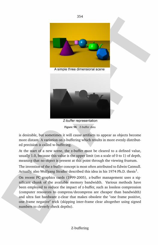
DRAF

T

354

Z-buffering

Figure 96 Z-buffer data

is desirable, but sometimes it will cause artifacts to appear as objects becomemore distant. A variation on z-buffering which results in more evenly distribut-ed precision is called w-buffering.

At the start of a new scene, the z-buffer must be cleared to a defined value,usually 1.0, because this value is the upper limit (on a scale of 0 to 1) of depth,meaning that no object is present at this point through the viewing frustum.

The invention of the z-buffer concept is most often attributed to Edwin Catmull.Actually, also Wolfgang Straßer described this idea in his 1974 Ph.D. thesis1.

On recent PC graphics cards (1999-2005), z-buffer management uses a sig-nificant chunk of the available memory bandwidth. Various methods havebeen employed to reduce the impact of z-buffer, such as lossless compression(computer resources to compress/decompress are cheaper than bandwidth)and ultra fast hardware z-clear that makes obsolete the "one frame positive,one frame negative" trick (skipping inter-frame clear altogether using signednumbers to cleverly check depths).

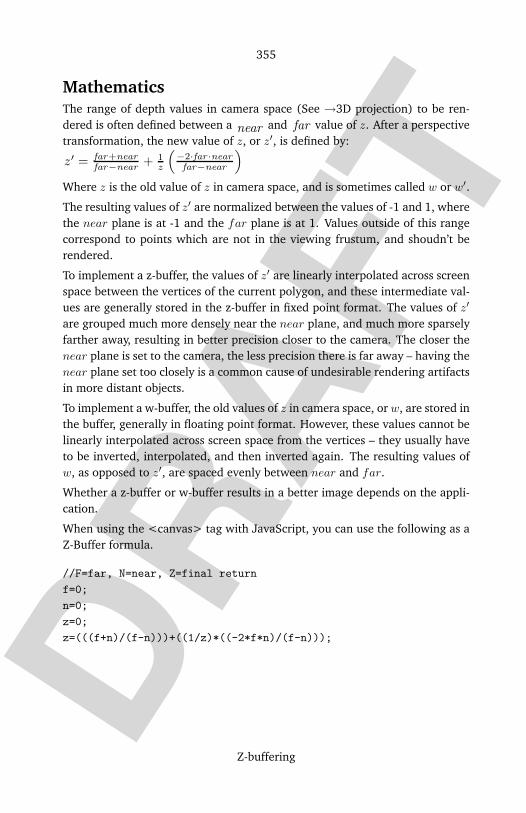
DRAF

T

355

Z-buffering

MathematicsThe range of depth values in camera space (See →3D projection) to be ren-dered is often defined between a

nearand far value of z. After a perspective

transformation, the new value of z, or z′, is defined by:

z′=

far+near

far−near+

1

z

(

−2·far ·near

far−near

)

Where z is the old value of z in camera space, and is sometimes called w or w′.

The resulting values of z′ are normalized between the values of -1 and 1, wherethe near plane is at -1 and the far plane is at 1. Values outside of this rangecorrespond to points which are not in the viewing frustum, and shoudn’t berendered.

To implement a z-buffer, the values of z′ are linearly interpolated across screenspace between the vertices of the current polygon, and these intermediate val-ues are generally stored in the z-buffer in fixed point format. The values of z′

are grouped much more densely near the near plane, and much more sparselyfarther away, resulting in better precision closer to the camera. The closer thenear plane is set to the camera, the less precision there is far away – having thenear plane set too closely is a common cause of undesirable rendering artifactsin more distant objects.

To implement a w-buffer, the old values of z in camera space, or w, are stored inthe buffer, generally in floating point format. However, these values cannot belinearly interpolated across screen space from the vertices – they usually haveto be inverted, interpolated, and then inverted again. The resulting values ofw, as opposed to z′, are spaced evenly between near and far.

Whether a z-buffer or w-buffer results in a better image depends on the appli-cation.

When using the <canvas> tag with JavaScript, you can use the following as aZ-Buffer formula.

//F=far, N=near, Z=final return

f=0;

n=0;

z=0;

z=(((f+n)/(f-n)))+((1/z)*((-2*f*n)/(f-n)));

DRAF

T

356

Z-fighting

See also

• Edwin Catmull – inventor of the z-buffer concept.• →3D computer graphics• →Irregular Z-buffer• Z-order

External links

• Learning to Love your Z-buffer386

• Alpha-blending and the Z-buffer387

NotesNote 1: see W.K. Giloi, J.L. Encarnação, W. Straßer. "The Giloi’s School ofComputer Graphics". Computer Graphics 35 4:12–16.

–>Source: http://en.wikipedia.org/wiki/Z-buffering

Principal Authors: PenguiN42, ToohrVyk, Zotel, Alfio, Solkoll, Zoicon5, Bookandcoffee

Z-fighting

Z-fighting is a phenomenon in 3D rendering that occurs when two or morecoplanar primitives have similar values in the Z-buffer, causing random partsof the primitives to be rendered. This problem is usually caused by floatingpoint round-off errors. Z-fighting is reduced by the use of a higher resolutiondepth buffer, by→W-buffering, or by simply moving the polygons further apart.

It is a relatively rare occurrence to encounter z-fighting while using a 24-bit Z-buffer. For example, with a 16-bit Z-buffer, at 10,000 units, resolving accuracyis only 1,800 units, meaning a point at 10,000 units away from the camera isgiven the same Z-buffer value as a point 11,799 units away. For comparison,resolving accuracy for a 24-bit Z-buffer is 6 units at the same distance.

As virtual world size increases, a greater likelihood exists that you will en-counter Z-fighting between primitives.

http://www.sjbaker.org/steve/omniv/love_your_z_buffer.html386

http://www.sjbaker.org/steve/omniv/alpha_sorting.html387

DRAF

T

357

Figure 97 Coplanar polygons

Source: http://en.wikipedia.org/wiki/Z-fighting

Principal Authors: Chentianran, Mhoskins, Rbrwr, Reedbeta, RJHall

DRAF

T

358

GNU Free Documentation LicenseVersion 1.2, November 2002

Copyright (C) 2000,2001,2002 Free Software Foundation, Inc. 51 Franklin St, Fifth Floor, Boston, MA 02110-1301USA Everyone is permitted to copy and distribute verbatim copies of this license document, but changing it is notallowed.

0. PREAMBLEThe purpose of this License is to make a manual, textbook, or other functional and useful document "free" in the senseof freedom: to assure everyone the effective freedom to copy and redistribute it, with or without modifying it, eithercommercially or noncommercially. Secondarily, this License preserves for the author and publisher a way to get creditfor their work, while not being considered responsible for modifications made by others.

This License is a kind of "copyleft", which means that derivative works of the document must themselves be free in thesame sense. It complements the GNU General Public License, which is a copyleft license designed for free software.

We have designed this License in order to use it for manuals for free software, because free software needs freedocumentation: a free program should come with manuals providing the same freedoms that the software does. Butthis License is not limited to software manuals; it can be used for any textual work, regardless of subject matteror whether it is published as a printed book. We recommend this License principally for works whose purpose isinstruction or reference.

1. APPLICABILITY AND DEFINITIONSThis License applies to any manual or other work, in any medium, that contains a notice placed by the copyrightholder saying it can be distributed under the terms of this License. Such a notice grants a world-wide, royalty-freelicense, unlimited in duration, to use that work under the conditions stated herein. The "Document", below, refers toany such manual or work. Any member of the public is a licensee, and is addressed as "you". You accept the license ifyou copy, modify or distribute the work in a way requiring permission under copyright law.

A "Modified Version" of the Document means any work containing the Document or a portion of it, either copiedverbatim, or with modifications and/or translated into another language.

A "Secondary Section" is a named appendix or a front-matter section of the Document that deals exclusively with therelationship of the publishers or authors of the Document to the Document’s overall subject (or to related matters)and contains nothing that could fall directly within that overall subject. (Thus, if the Document is in part a textbook ofmathematics, a Secondary Section may not explain any mathematics.) The relationship could be a matter of historicalconnection with the subject or with related matters, or of legal, commercial, philosophical, ethical or political positionregarding them.

The "Invariant Sections" are certain Secondary Sections whose titles are designated, as being those of Invariant Sec-tions, in the notice that says that the Document is released under this License. If a section does not fit the abovedefinition of Secondary then it is not allowed to be designated as Invariant. The Document may contain zero InvariantSections. If the Document does not identify any Invariant Sections then there are none.

The "Cover Texts" are certain short passages of text that are listed, as Front-Cover Texts or Back-Cover Texts, in thenotice that says that the Document is released under this License. A Front-Cover Text may be at most 5 words, and aBack-Cover Text may be at most 25 words.

A "Transparent" copy of the Document means a machine-readable copy, represented in a format whose specification isavailable to the general public, that is suitable for revising the document straightforwardly with generic text editorsor (for images composed of pixels) generic paint programs or (for drawings) some widely available drawing editor,and that is suitable for input to text formatters or for automatic translation to a variety of formats suitable for inputto text formatters. A copy made in an otherwise Transparent file format whose markup, or absence of markup, hasbeen arranged to thwart or discourage subsequent modification by readers is not Transparent. An image format is notTransparent if used for any substantial amount of text. A copy that is not "Transparent" is called "Opaque".

Examples of suitable formats for Transparent copies include plain ASCII without markup, Texinfo input format, LaTeXinput format, SGML or XML using a publicly available DTD, and standard-conforming simple HTML, PostScript or PDFdesigned for human modification. Examples of transparent image formats include PNG, XCF and JPG. Opaque formatsinclude proprietary formats that can be read and edited only by proprietary word processors, SGML or XML for whichthe DTD and/or processing tools are not generally available, and the machine-generated HTML, PostScript or PDFproduced by some word processors for output purposes only.

The "Title Page" means, for a printed book, the title page itself, plus such following pages as are needed to hold, legibly,the material this License requires to appear in the title page. For works in formats which do not have any title page as

DRAF

T

359

such, "Title Page" means the text near the most prominent appearance of the work’s title, preceding the beginning ofthe body of the text.

A section "Entitled XYZ" means a named subunit of the Document whose title either is precisely XYZ or contains XYZin parentheses following text that translates XYZ in another language. (Here XYZ stands for a specific section namementioned below, such as "Acknowledgements", "Dedications", "Endorsements", or "History".) To "Preserve the Title"of such a section when you modify the Document means that it remains a section "Entitled XYZ" according to thisdefinition.

The Document may include Warranty Disclaimers next to the notice which states that this License applies to theDocument. These Warranty Disclaimers are considered to be included by reference in this License, but only as regardsdisclaiming warranties: any other implication that these Warranty Disclaimers may have is void and has no effect onthe meaning of this License.

2. VERBATIM COPYINGYou may copy and distribute the Document in any medium, either commercially or noncommercially, provided thatthis License, the copyright notices, and the license notice saying this License applies to the Document are reproducedin all copies, and that you add no other conditions whatsoever to those of this License. You may not use technicalmeasures to obstruct or control the reading or further copying of the copies you make or distribute. However, you mayaccept compensation in exchange for copies. If you distribute a large enough number of copies you must also followthe conditions in section 3.

You may also lend copies, under the same conditions stated above, and you may publicly display copies.

3. COPYING IN QUANTITYIf you publish printed copies (or copies in media that commonly have printed covers) of the Document, numberingmore than 100, and the Document’s license notice requires Cover Texts, you must enclose the copies in covers thatcarry, clearly and legibly, all these Cover Texts: Front-Cover Texts on the front cover, and Back-Cover Texts on theback cover. Both covers must also clearly and legibly identify you as the publisher of these copies. The front covermust present the full title with all words of the title equally prominent and visible. You may add other material on thecovers in addition. Copying with changes limited to the covers, as long as they preserve the title of the Document andsatisfy these conditions, can be treated as verbatim copying in other respects.

If the required texts for either cover are too voluminous to fit legibly, you should put the first ones listed (as many asfit reasonably) on the actual cover, and continue the rest onto adjacent pages.

If you publish or distribute Opaque copies of the Document numbering more than 100, you must either include amachine-readable Transparent copy along with each Opaque copy, or state in or with each Opaque copy a computer-network location from which the general network-using public has access to download using public-standard networkprotocols a complete Transparent copy of the Document, free of added material. If you use the latter option, youmust take reasonably prudent steps, when you begin distribution of Opaque copies in quantity, to ensure that thisTransparent copy will remain thus accessible at the stated location until at least one year after the last time youdistribute an Opaque copy (directly or through your agents or retailers) of that edition to the public.

It is requested, but not required, that you contact the authors of the Document well before redistributing any largenumber of copies, to give them a chance to provide you with an updated version of the Document.

4. MODIFICATIONSYou may copy and distribute a Modified Version of the Document under the conditions of sections 2 and 3 above,provided that you release the Modified Version under precisely this License, with the Modified Version filling the roleof the Document, thus licensing distribution and modification of the Modified Version to whoever possesses a copy ofit. In addition, you must do these things in the Modified Version:

A. Use in the Title Page (and on the covers, if any) a title distinct from that of the Document, and from those ofprevious versions (which should, if there were any, be listed in the History section of the Document). You may usethe same title as a previous version if the original publisher of that version gives permission.

B. List on the Title Page, as authors, one or more persons or entities responsible for authorship of the modificationsin the Modified Version, together with at least five of the principal authors of the Document (all of its principalauthors, if it has fewer than five), unless they release you from this requirement.

C. State on the Title page the name of the publisher of the Modified Version, as the publisher.D. Preserve all the copyright notices of the Document.E. Add an appropriate copyright notice for your modifications adjacent to the other copyright notices.F. Include, immediately after the copyright notices, a license notice giving the public permission to use the Modified

Version under the terms of this License, in the form shown in the Addendum below.

DRAF

T

360

G. Preserve in that license notice the full lists of Invariant Sections and required Cover Texts given in the Document’slicense notice.

H. Include an unaltered copy of this License.I. Preserve the section Entitled "History", Preserve its Title, and add to it an item stating at least the title, year, new

authors, and publisher of the Modified Version as given on the Title Page. If there is no section Entitled "History" inthe Document, create one stating the title, year, authors, and publisher of the Document as given on its Title Page,then add an item describing the Modified Version as stated in the previous sentence.

J. Preserve the network location, if any, given in the Document for public access to a Transparent copy of the Docu-ment, and likewise the network locations given in the Document for previous versions it was based on. These maybe placed in the "History" section. You may omit a network location for a work that was published at least fouryears before the Document itself, or if the original publisher of the version it refers to gives permission.

K. For any section Entitled "Acknowledgements" or "Dedications", Preserve the Title of the section, and preserve in thesection all the substance and tone of each of the contributor acknowledgements and/or dedications given therein.

L. Preserve all the Invariant Sections of the Document, unaltered in their text and in their titles. Section numbers orthe equivalent are not considered part of the section titles.

M. Delete any section Entitled "Endorsements". Such a section may not be included in the Modified Version.N. Do not retitle any existing section to be Entitled "Endorsements" or to conflict in title with any Invariant Section.O. Preserve any Warranty Disclaimers.

If the Modified Version includes new front-matter sections or appendices that qualify as Secondary Sections and containno material copied from the Document, you may at your option designate some or all of these sections as invariant.To do this, add their titles to the list of Invariant Sections in the Modified Version’s license notice. These titles must bedistinct from any other section titles.

You may add a section Entitled "Endorsements", provided it contains nothing but endorsements of your ModifiedVersion by various parties–for example, statements of peer review or that the text has been approved by an organizationas the authoritative definition of a standard.

You may add a passage of up to five words as a Front-Cover Text, and a passage of up to 25 words as a Back-CoverText, to the end of the list of Cover Texts in the Modified Version. Only one passage of Front-Cover Text and oneof Back-Cover Text may be added by (or through arrangements made by) any one entity. If the Document alreadyincludes a cover text for the same cover, previously added by you or by arrangement made by the same entity youare acting on behalf of, you may not add another; but you may replace the old one, on explicit permission from theprevious publisher that added the old one.

The author(s) and publisher(s) of the Document do not by this License give permission to use their names for publicityfor or to assert or imply endorsement of any Modified Version.

5. COMBINING DOCUMENTSYou may combine the Document with other documents released under this License, under the terms defined in section4 above for modified versions, provided that you include in the combination all of the Invariant Sections of all of theoriginal documents, unmodified, and list them all as Invariant Sections of your combined work in its license notice,and that you preserve all their Warranty Disclaimers.

The combined work need only contain one copy of this License, and multiple identical Invariant Sections may bereplaced with a single copy. If there are multiple Invariant Sections with the same name but different contents, makethe title of each such section unique by adding at the end of it, in parentheses, the name of the original author orpublisher of that section if known, or else a unique number. Make the same adjustment to the section titles in the listof Invariant Sections in the license notice of the combined work.

In the combination, you must combine any sections Entitled "History" in the various original documents, formingone section Entitled "History"; likewise combine any sections Entitled "Acknowledgements", and any sections Entitled"Dedications". You must delete all sections Entitled "Endorsements."

6. COLLECTIONS OF DOCUMENTSYou may make a collection consisting of the Document and other documents released under this License, and replacethe individual copies of this License in the various documents with a single copy that is included in the collection,provided that you follow the rules of this License for verbatim copying of each of the documents in all other respects.

You may extract a single document from such a collection, and distribute it individually under this License, providedyou insert a copy of this License into the extracted document, and follow this License in all other respects regardingverbatim copying of that document.

DRAF

T

361

7. AGGREGATION WITH INDEPENDENT WORKSA compilation of the Document or its derivatives with other separate and independent documents or works, in or ona volume of a storage or distribution medium, is called an "aggregate" if the copyright resulting from the compilationis not used to limit the legal rights of the compilation’s users beyond what the individual works permit. When theDocument is included in an aggregate, this License does not apply to the other works in the aggregate which are notthemselves derivative works of the Document.

If the Cover Text requirement of section 3 is applicable to these copies of the Document, then if the Document is lessthan one half of the entire aggregate, the Document’s Cover Texts may be placed on covers that bracket the Documentwithin the aggregate, or the electronic equivalent of covers if the Document is in electronic form. Otherwise they mustappear on printed covers that bracket the whole aggregate.

8. TRANSLATIONTranslation is considered a kind of modification, so you may distribute translations of the Document under the termsof section 4. Replacing Invariant Sections with translations requires special permission from their copyright holders,but you may include translations of some or all Invariant Sections in addition to the original versions of these InvariantSections. You may include a translation of this License, and all the license notices in the Document, and any WarrantyDisclaimers, provided that you also include the original English version of this License and the original versions ofthose notices and disclaimers. In case of a disagreement between the translation and the original version of thisLicense or a notice or disclaimer, the original version will prevail.

If a section in the Document is Entitled "Acknowledgements", "Dedications", or "History", the requirement (section 4)to Preserve its Title (section 1) will typically require changing the actual title.

9. TERMINATIONYou may not copy, modify, sublicense, or distribute the Document except as expressly provided for under this License.Any other attempt to copy, modify, sublicense or distribute the Document is void, and will automatically terminateyour rights under this License. However, parties who have received copies, or rights, from you under this License willnot have their licenses terminated so long as such parties remain in full compliance.

10. FUTURE REVISIONS OF THIS LICENSEThe Free Software Foundation may publish new, revised versions of the GNU Free Documentation License from timeto time. Such new versions will be similar in spirit to the present version, but may differ in detail to address newproblems or concerns. See http://www.gnu.org/copyleft/.

Each version of the License is given a distinguishing version number. If the Document specifies that a particularnumbered version of this License "or any later version" applies to it, you have the option of following the terms andconditions either of that specified version or of any later version that has been published (not as a draft) by the FreeSoftware Foundation. If the Document does not specify a version number of this License, you may choose any versionever published (not as a draft) by the Free Software Foundation.

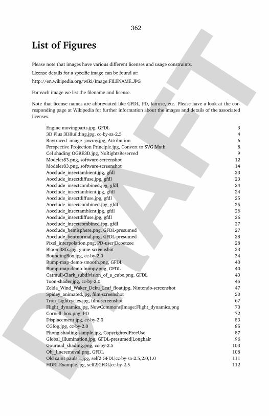
DRAF

T

362

List of Figures

Please note that images have various different licenses and usage constraints.

License details for a specific image can be found at:

http://en.wikipedia.org/wiki/Image:FILENAME.JPG

For each image we list the filename and license.

Note that license names are abbreviated like GFDL, PD, fairuse, etc. Please have a look at the cor-responding page at Wikipedia for further information about the images and details of the associatedlicenses.

Engine movingparts.jpg, GFDL 33D Plus 3DBuilding.jpg, cc-by-sa-2.5 4Raytraced_image_jawray.jpg, Attribution 6Perspective Projection Principle.jpg, Convert to SVG|Math 8Cel shading OGRE3D.jpg, NoRightsReserved 9Modeler83.png, software-screenshot 12Modeler83.png, software-screenshot 14Aocclude_insectambient.jpg, gfdl 23Aocclude_insectdiffuse.jpg, gfdl 23Aocclude_insectcombined.jpg, gfdl 24Aocclude_insectambient.jpg, gfdl 24Aocclude_insectdiffuse.jpg, gfdl 25Aocclude_insectcombined.jpg, gfdl 25Aocclude_insectambient.jpg, gfdl 26Aocclude_insectdiffuse.jpg, gfdl 26Aocclude_insectcombined.jpg, gfdl 27Aocclude_hemisphere.png, GFDL-presumed 27Aocclude_bentnormal.png, GFDL-presumed 28Pixel_interpolation.png, PD-user|Dcoetzee 28Bloom38fx.jpg, game-screenshot 33BoundingBox.jpg, cc-by-2.0 34Bump-map-demo-smooth.png, GFDL 40Bump-map-demo-bumpy.png, GFDL 40Catmull-Clark_subdivision_of_a_cube.png, GFDL 43Toon-shader.jpg, cc-by-2.0 45Zelda_Wind_Waker_Deku_Leaf_float.jpg, Nintendo-screenshot 47Spidey_animated.jpg, film-screenshot 50Tron_Lightcycles.jpg, film-screenshot 67Flight_dynamics.jpg, NowCommons|Image:Flight_dynamics.png 70Cornell_box.png, PD 72Displacement.jpg, cc-by-2.0 83CGfog.jpg, cc-by-2.0 85Phong-shading-sample.jpg, CopyrightedFreeUse 87Global_illumination.jpg, GFDL-presumed|Longhair 96Gouraud_shading.png, cc-by-2.5 103Obj_lineremoval.png, GFDL 108Old saint pauls 1.jpg, self2|GFDL|cc-by-sa-2.5,2.0,1.0 111HDRI-Example.jpg, self2|GFDL|cc-by-2.5 112

DRAF

T

363

Old saint pauls 2.jpg, FeaturedPicture 113Grand Canyon HDR imaging.jpg, self2|GFDL|cc-by-2.5 114Farcryhdr.jpg, game-screenshot 116Farcrynohdr.jpg, game-screenshot 117Hl2hdrcomparison.jpg, game-screenshot 118Dodsourceinside1.jpg, game-screenshot 120Dodsourceinside2.jpg, game-screenshot 121Dodsourceoutside1.jpg, game-screenshot 121Dodsourceoutside2.jpg, game-screenshot 122Isosurface_on_molecule.jpg, CopyrightedFreeUseProvided 135LambertCosineLaw1.png, PD-self 139LambertCosineLaw2.png, PD-self 140Metaballs.gif, GFDL 146MotionCapture.jpg, GFDL-self 153Painters_problem.png, GFDL 163Normal map example.png, cc-by-sa 164OpenGL_Logo.jpg, logo|Computer software logos 168Painter’s_algorithm.png, NowCommonsThis 187Painters_problem.png, GFDL 187Fear-pmapping1.jpg, game-screenshot 189Fear-pmapping2.jpg, game-screenshot 189Fear-pmapping3.jpg, game-screenshot 190particle_sys_fire.jpg 191particle_sys_galaxy.jpg 192particle_sys_trail.jpg 192Phong-shading-sample.jpg, CopyrightedFreeUse 201Caustics.jpg, cc-by-2.0 202Procedural Texture.jpg, GFDL 219Radiosity.png, PD-user|Wapcaplet 246Raytraced_image_jawray.jpg, Attribution 251Raytracing reflection.png, PD-self 252Spoon_fi.jpg, GFDL-self 263cube_mapped_reflection_example.jpg 264Cube_mapped_reflection_example_2.JPG, PD-self 2657fin.png, GFDL-self 3023noshadow.png, GFDL-self 3031light.png, GFDL-self 3042shadowmap.png, GFDL-self 3054overmap.png, GFDL-self 3065failed.png, GFDL-self 3076black.png, GFDL-self 3077fin.png, GFDL-self 308Cad-fm01s.gif, GFDL-self 315Catmull-Clark_subdivision_of_a_cube.png, GFDL 325Scattering-example.jpg, cc-by-2.0 328SurfaceNormalDrawing.PNG, PD-ineligible 330TextureMapping.png, cc-by-2.0 334Doom3Marine.jpg, game-screenshot 337Quake3Screenshot.jpg, game-screenshot 338utah_teapot.png 339Melitta teapot.png, PD 340

DRAF

T

364

CTSkullImage.png, PD-self 345CTWristImage.png, PD-self 346Z-buffer.jpg, cc-by-2.0 354Z-fighting.png, PD-self 357

DRAF

T

365

Index

.kkrieger 21516-bit 35319th century 452006-05-16 4220th century 4624-bit 353, 35627 october 2962d computer graphics 2, 1683-sphere 24532-bit 3533d animation 77, 1363dc 282, 2843d computer graphics 11, 22, 22, 42, 51, 67,

73, 74, 76, 85, 87, 88, 95, 109, 131, 148,149, 152, 163, 164, 168, 187, 198, 200,206, 211, 222, 245, 252, 252, 266, 279,281, 284, 292, 302, 309, 317, 322, 327,331, 343, 344, 350, 356

3d display 3503dfx 65, 943d geometric model 913d geometry 1053d graphics 41, 94, 2813d graphics card 3533dlabs 169, 1763d model 10, 132, 1973d modeler 10, 14, 153d modeling 383d modelling 3423d motion controller 113d projection 10, 3553d rendering 33d scanner 2083d studio 53d studio max 12, 56, 158, 194, 209, 245,

3414d 2406dof 1566 march 2948-bit 353oban star-racers 50okami 48

aaabb 289absorption 248acceleration 153acis 314acm press 104acm transactions on graphics 147, 194, 212

acquisition 92activision 166actor 331actual state 259adobe illustrator 286afterburn 194aki ross 331algorithm 15, 26, 67, 91, 92, 95, 148, 188,

218, 245, 281, 284algorithmic 79algorithms 35aliasing 27, 67, 272almost everywhere 330alpha blending 59, 170alpha channel 283ambient occlusion 3, 10, 130anaglyph image 10analysis 92anatomical position 343anatomy 343angle 153, 241anim8or 13animation 11, 129, 131, 132, 161, 312, 316animation#styles and techniques of animation

51animation control 132animator 132anime 46anisotropic 150anisotropic filtering 31, 333anthony a. apodaca 148anti-aliasing 134, 151, 255antialiasing 272, 333api 145, 178, 183, 186, 322apple computer 169appleseed 48applied mathematics 92arcade game 86architecture review board 62array 287, 293arthur appel 254artificial intelligence 74, 74artist 132art of illusion 13, 44ascendant 344assembly modelling 314associativity 241astrology 344ati technologies 64, 95, 169atomic betty 49

DRAF

T

366

august 23 124august 9 124autocad 209, 286, 317, 341autodesk 11, 12autodessys, inc. 13auto modellista 48autostereogram 11aux 172avionics 181

bb-spline 326, 326, 326bandwidth 354barycentric coordinates (mathematics) 211batch 293bbc 77beam tracing 67, 96, 259beos 341beyblade: the movie - fierce battle 48bi-directional path tracing 147, 195bidirectional reflectance distribution function

274bilinear filtering 333bilinear interpolation 29, 335binary space partitioning 250binocular 252biomedical computing 92birch 215bit 282bitmap 28bitmap textures 267black body 138blinn–phong shading model 104, 202blinn-phong shading 318bloom (shader effect) 122bmrt 90bomberman generation 48bomberman jetters 48bone 135boolean 68boundary representation 87, 312, 316bounding sphere 36bounding volume 344bounding volume hierarchies 35box modeling 207box splines 326brain 131branch 300brazil r/s 7bresenham’s line algorithm 211, 335brian paul 145brightness 33, 321brl-cad 69, 204, 259, 317

buck 65 344buffer 353bugs bunny 77bui tuong phong 198, 200, 200, 200, 202bump mapping 1, 9, 15, 80, 83, 84, 143,

164, 166, 188, 190, 197, 267, 296, 335bumpmapping 217butterfly 326byte 321

cc

+ 173, 178, 183, 286, 288c4 engine 56cache 151cache coherency 269cache memory 285cad 8, 68, 69, 79, 222, 316calculation 131calculus 275call of duty 2 166caltech 93cam 8canada’s worst driver 49carmack’s reverse 310, 322cartoon 45cass everitt 322casting 312cat 28catia 317caustics 7cel damage 47, 48celluloid 46cellulose acetate 46cgl 174cg programming language 56change state 87character animation 51charts on so(3) 244chemistry 136chirality 226chrominance 112cinema 4d 13cinematography 111, 350circle 36, 91, 140circumference 5clanlib 205class of the titans 49clifford algebra 244clip mapping 144clipping (computer graphics) 106collinear 240, 241collision detection 35

DRAF

T

367

color 76, 91, 351color buffer 321comic book 45comm. acm 39command & conquer: tiberian series 351comparison of direct3d and opengl 80, 176compiler 217compiz 63compositing 8, 279computation 247computational fluid dynamics 135computational geometry 34, 91, 212, 316computed axial tomography 316computer 14, 15, 258computer-aided design 91, 92, 93computer-generated imagery 11, 78, 143, 279computer and video games 15, 109, 141,

152, 257, 266, 350computer animation 51, 76, 131, 152, 158,

210computer cluster 298computer display 119computer game 10, 15, 149, 243, 304, 309computer games 33computer generated image 218computer graphics 16, 22, 25, 33, 34, 39,

40, 45, 54, 75, 76, 85, 88, 89, 91, 92, 100,103, 105, 111, 115, 135, 137, 141, 146,196, 197, 203, 210, 213, 213, 244, 248,262, 312, 316, 321, 325, 332, 333, 338,353, 353

computer history museum 340computer program 292computer programming 54, 100, 141computer science 92computer software 58concave 338cone tracing 27, 96, 259consortium 180constraints 136constructive solid geometry 4, 87, 313continuous function 272contrast ratio 33conversion between quaternions and euler an-

gles 244convex 250convex hull 37coordinate 5, 350coordinate rotation 244coordinates 339, 342coreldraw 286cornell box 342cornell university 71, 245

cosine 138, 242cosmo 3d 179, 185covering map 245c programming language 52, 59, 97, 99, 99cpu 215crazyracing kartrider 48creative labs 42, 322cross-platform 168, 182cross platform 98cross product 329crowd psychology 74crystal space 54crytek 166cube 243, 341cube map 75, 265cube mapping 264, 266cuboid 36, 68curve 243curvilinear coordinates 330cut scene 213cylinder 36

dd.i.c.e. 49d3dx 341dark cloud 2 47, 48darwyn peachey 297data structure 134, 286, 287datatype 293david s. elbert 297day of defeat: source 120decal 335december 24 123delilah and julius 49demo effect 147demo effects 84demoscene 214density 135, 351depth buffer 289, 321, 356depth of field 7, 267deus ex: invisible war 33, 166device driver 175diameter 140diffraction 257diffuse inter-reflection 96diffuse interreflection 203diffuse reflection 137, 138, 320, 345diffusion 292digital 2digital camera 118digital content creation 56, 300digital equipment corporation 178digital image 91, 266

DRAF

T

368

digital images 112digital puppetry 159dimension 91direct3d 3, 10, 58, 95, 128, 168, 175, 176,

208, 285, 322, 341direct3d vs. opengl 168directdraw 80directdraw surface 284direct illumination 245directly proportional 138directx 10, 53, 55, 79, 84, 94, 123, 123, 205,

273, 281, 323directx graphics 80disney’s california adventure 77displacement mapping 41, 41, 148, 166, 190display generator 92distance fog 86distributed ray tracing 27, 67, 259doctor who 331dodecahedron 341doo-sabin 326doom 250doom 3 33, 42, 144, 144, 166, 214, 309,

322, 336doom engine 250dot product 137, 199dragon ball z: budokai 2 48dragon booster 49dragon quest viii 48, 49duck dodgers 49duke nukem 3d 250dust 350dvd 274dxf 209dxt5 1dynamical simulation 36dynamic link library 82dynamic range 111

eearth science 15edge modeling 38educational film 250, 254edwin catmull 43, 325, 335, 354, 356eidos interactive 166elbow 88ellipse 286elmsford, new york 249, 254embedded device 180emergent behavior 74emission spectrum 71emulate 80enemy territory: quake wars 144, 144

energy 140engineering 92engineering drawing 314, 316entertainment 92environment map 23environment mapping 134eovia 13epic games 166epic megagames 116eric veach 147euclidean geometry 206euclidean space 206euler angle 243euler angles 69, 244, 288euler characteristic 87evans & sutherland 285execute buffer 59extrusion 312eye 246e3 116

ff.e.a.r. 189, 190f. kenton musgrave 297facet 313facial motion capture 160fad 46fahrenheit graphics api 66fairly oddparents 49family guy 49farbrausch 214far cry 54, 166farcry 117fear effect 46february 2 173field of view 25file format 208film 73, 89final-render 7final fantasy: the spirits within 213, 331final gathering 130finding nemo 77finite difference 313finite element 268finite element analysis 210finite state machine 59first-person shooter 215fisheye lens 263fixed-point 211flat shading 9, 104flight dynamics 70flight simulator 149floating point 16, 112, 123, 180, 211, 355,

DRAF

T

369

356fltk 102, 172, 205fluid flow 135fmv game 213fog 299, 350formz 13fortran 90 173forward kinematic animation 4, 131fourcc 282fractal 91, 213, 218fractal landscape 196, 217fraction (mathematics) 211fragment 300frame buffer 89, 106, 340framebuffer 294frame rate 209frank crow 322freeform surface modelling 314freeglut 182free software 182, 185frustum 344, 355full motion video 213full screen effect 112, 119functional programming 214funky cops 49futurama 48, 49fxt1 284

gg.i. joe: sigma 6 49gamecube 123game developers conference 218game physics 191game programmer 42gamma correction 112gamut 120gaussian distribution 319, 319geforce 62, 89geforce 2 41geforce 256 61geforce fx 124, 129geometric 1geometrical optics 252geometric primitive 105geometric space 91geometry 343geophysics 136ghost in the shell: s.a.c. 2nd gig 48ghost in the shell: stand alone complex 48gigabytes 215glass cockpit 181glee 172, 173glew 172, 173

glide api 10, 65global illumination 22, 76, 130, 130, 203,

245, 256, 259, 273glossy 76glsl 169, 176, 176, 295, 300glu 102, 172, 176, 182glucose transporter 182glui 101, 172, 182glut 101, 102, 102, 172, 174, 176, 341glx 174gnu gpl 185gollum 143, 159google earth 56, 110gouraud shading 9, 32, 32, 88, 201gpu 348gradient 330grand theft auto 3 86granite 218granularity 296graphic art 2graphics 11graphics card 3, 10, 22, 56, 80, 89, 94, 106,

124, 208, 268, 285, 299, 332, 336graphics cards 124graphics hardware 105graphics pipeline 32, 89, 109, 169, 176, 277,

299graphics processing unit 52, 97, 216, 299graph theory 343gravity 73grayscale 164green 72gregory ward 111greg ward 116group dynamics 74gtk 205gui 205, 287gundam seed 49gungrave 49

hhalf-life 2 166half-life 2: lost coast 116, 118half precision 112halo 2 141, 166hardware 10, 134, 321, 353hardware acceleration 79, 336harvest moon: save the homeland 49heat transfer 96heightfield 110, 291heightmap 40, 83, 84hemicube 247henrik wann jensen 203

DRAF

T

370

hewlett-packard 174hidden face removal 108hidden line removal 79, 109high-definition 214high dynamic range imaging 116, 130high dynamic range rendering 33, 34, 113high level shader language 80history of 3d graphics 11hlsl 295homogeneous coordinates 20hoops3d 10horoscope 344hot wheels highway 35 world race 48html 39hue 246human eye 119hypotenuse 341

ii-deas 317ian bell 217ibm 174, 178, 185icosahedron 208, 341id software 42, 144, 144, 166, 214, 322, 336ieee transactions on computers 104ihv 64illusion 321image 103, 266image-based lighting 23image compression 281image order 248image plane 26image processing 178image resolution 272immediate-mode rendering 174implementation 300implicit surface 4in-joke 338infinitesimal 244injection moulding 312innocence: ghost in the shell 48input device 173integer 123, 321integral 247intel 169, 178, 185, 218interaction point 343interactive manipulation 132interpolation 326invader zim 50inverse kinematic animation 4, 88, 132inverse kinematics 132, 136, 208invisibility 222iris 64, 119

iris inventor 175iris performer 175irradiance 138irregular z-buffer 356irrlicht 10isocontour 135isometric projection 19isotropic 150ivan sutherland 285

jjade cocoon 217jaggies 272james d. foley 251james h. clark 92japan 48jar-jar binks 159jar jar binks 316java 3d 10, 173java opengl 176javascript 355jet set radio 46, 49jet set radio future 46jim blinn 9, 146, 340jim henson 77jitendra malik 128jogl 173johann heinrich lambert 138john carmack 42, 59, 144, 310, 322, 329joint 136jsr 184 10july 28 42july 29 42

kkd-tree 134ken perlin 196, 297kermit the frog 77keyframing 5khronos group 169, 180killer 7 48, 49kilobytes 215kinematic decoupling 132kinematics 132kirby: right back at ya! 50klonoa 2 47, 49kluge 79kml 57knuckle 88kobbelt 326kurt akeley 54, 169

DRAF

T

371

ll-system 217l2 cache 216lambert’s cosine law 138, 331lambertian 165lambertian diffuse lighting model 103lambertian reflectance 76lance williams 151, 302larry gritz 148laser 258latin 149, 343lazy evaluation 214led 152lego exo-force 48, 51lenna 73, 73, 342lens flare 7leonidas j. guibas 147level set 135lgpl 205light 75, 76, 203, 252, 317, 321, 327light absorption 292lighting 266, 350lighting model 295lightmap 214light probe 263light tracing 195light transport theory 130lightwave 5, 14, 209light weight java game library 177line-sphere intersection 259linear 353linear algebra 166, 275linear interpolation 29linked list 287linux 58, 63, 98, 168, 173lipschitz continuous 330list of 3d artists 11list of cel-shaded video games 48, 51list of software patents 42list of vector graphics markup languages 57live & kicking 77load balancing 294logarithmic 258logical operator 53logluv tiff 113looney tunes: back in action 77lord of the rings 143lorentz group 240lossless compression 354lossy data compression 1low poly 143, 165luminance 112, 137, 138luminous energy 140

mm. c. escher 87m. e. newell 163machinima 77, 78mac os 58, 168mac os x 58, 63, 174magic eye 11magnetic resonance imaging 316manifold 207maple 215marble 218, 327marching cubes 136, 147, 351marc levoy 347mark kilgard 297, 322massive (animation) 74match moving 14, 153, 161mathematical 131mathematical applications group, inc. 249,

254matrox 64maxon 13maya 56medical image processing 91medical imaging 135megaman nt warrior 50mega man x7 49mega man x command mission 49melitta 340mental ray 7, 13, 273mesa 3d 173, 176mesh 43, 82, 213, 294metaball 194metal 218metal gear acid 2 48, 49metal gear solid 3 123meteorology 136metropolis-hastings algorithm 147metropolis light transport 96, 256michael abrash 329micropolygon 84microscope 252microsoft 62, 79, 123, 123, 128, 169, 178,

185, 281, 300microsoft corporation 58microsoft train simulator 341microsoft windows 168, 174, 341midedge 326milk 327milkshape 3d 13milling 312mimd 348minigl 94minimax 163

DRAF

T

372

mip-mapping 333mipmap 56, 101, 180mipmapping 166mit license 145mobile phone 180mode 7 250modelview matrix 92monster house 50monster rancher 49monsters inc. 341monte carlo method 23, 147, 203motion blur 7, 267motion capture 77, 78, 132motion control photography 279mountain view, california 340movies 266movie studio 159multi-agent system 74multimedia 92multi pass rendering 296multiprocessing 292muppet 77

nneed for speed underground 2 123network transparency 174new line cinema 74news 175newtek 12new york 249, 254new zealand 111, 113nintendo 58, 123nintendo 64 85noctis 217noise 218non-photorealistic rendering 45, 268nonlinear programming 132normalize 355normal map 282normal mapping 41, 83, 84, 143, 188normal vector 25, 137novalogic 351nsopengl 174numerical 218numerical instability 79nunchaku 158nurbs 4, 101, 143, 165, 206, 326nvidia 1, 52, 64, 89, 95, 117, 124, 169, 299,

300, 322nvidia scene graph 10nx (unigraphics) 317

oobb 289obb tree 35obj 209object-oriented 178object-oriented model 91object oriented 183octahedron 341october 2005 294octree 110, 291, 349ogre 10old saint paul’s 111, 113on the fly 213opcodes 59openal 176open directory project 178openexr 113opengl 3, 10, 20, 32, 53, 55, 58, 80, 84, 92,

93, 94, 94, 98, 99, 100, 101, 145, 145, 178,180, 182, 183, 186, 205, 208, 257, 273,281, 285, 300, 308, 322, 323, 332, 337, 341+ 175

opengl arb 97, 98, 145opengl architecture review board 169, 177opengl es 10, 59, 169, 176opengl performer 173, 178, 184opengl shading language 10openglut 182open inventor 178, 291openml 205openrt 257, 262openscenegraph 10, 173opensg 10opensl es 176open source 95, 145, 145, 168, 173, 179,

185, 205open standard 1, 58operating system 58, 173, 182operating systems 79operation 68optical axis 343optical coating 258optical resonator 258optics 76, 343orientation 244orthogonal 243orthogonal matrix 70, 243orthographic projection 101, 305oslo 258out-of-order execution 216

pp. g. tait 224

DRAF

T

373

paging 82paint 76painter’s algorithm 110, 164, 273, 289, 353panda3d 11panoscan 113parallax 190parallax mapping 41, 83, 84, 166, 166parameter 68, 293parasolid 314parietal bone 343partial derivative 330particle physics 343particle system 7, 74, 82particle systems ltd 191pat hanrahan 26path tracing 96paul debevec 111, 116, 266paul e. debevec 128paul heckbert 26pdf 127pencil tracing 259pentium 329performance capture 160perl 173perlin noise 222, 297perpendicular 329personal computer 15personal computers 90perspective distortion 19, 22perspective projection 8, 305perspective transform 355pharmacology 136phigs 174philip mittelman 254philipp slusallek 259phonemes 5phong reflection model 8, 32, 32, 39, 200,

201, 202, 285, 318phong shading 8, 9, 22, 32, 32, 39, 40, 88,

104, 137, 197, 197, 198, 200, 206photograph 131photography 2photon 140, 248, 253photon mapping 72, 76, 96, 256, 256, 259photoshopping 205physical law 88physical simulation 208pixar 13, 43, 90, 143, 273, 298, 302, 327pixel 26, 32, 40, 89, 106, 197, 198, 250,

281, 285, 303, 333, 335, 350, 353pixel buffer 321pixel image editor 113pixels 131, 332, 340

pixel shaders 80, 348pixologic 13planar 163plasma displays 119platonic solid 341playstation 2 123playstation 3 54, 56, 58, 123, 168, 181, 214,

216, 216playstation portable 56plib 173plug-in 194plugin 11poincaré group 240pointer 99point spread function 257polarized glasses 11polygon 5, 14, 25, 26, 36, 87, 103, 134, 148,

163, 187, 206, 211, 211, 211, 329, 343,351, 355

polygonal modeling 4polygon mesh 210, 211polygon modeling 211polygons 206polyhedron 36, 43, 343polynomial 91polytope 36polyurethane 137portal rendering 110portmanteau 331, 350poser 14position 153post-processing 292pov-ray 5, 7, 13, 72, 259, 341povray 96poweranimator 64powerwall 259pre-rendered 277pro/engineer 317procedural animation 217procedural generation 222procedural texture 217procedural textures 267procedure 68product visualization 312profile 180programmer 10, 41programming 52programming language 292, 298projection matrix 92puppeteer 78puppeteers 77puppets 78pyramid 222

DRAF

T

374

pythagorean theorem 341

qqsdk 10quadric 101quadrilateral 44, 211quadtree 291quake 69, 94, 209quake iii 336quake iii arena 61quartz compositor 63quaternion 223, 244quaternions 288quesa 10

rradeon 62radian 242radiance 23, 112, 138, 140radiance (software) 259radiation exposure 249, 254radiative heat transfer 245radiosity 7, 76, 96, 198, 212, 214, 253, 256,

259, 268, 270, 273ram 216, 321randima fernando 297randi rost 297rapid prototyping 312, 316raster graphics 266raster image 105rasterisation 163rasterization 105, 105, 106, 106, 106, 106,

133, 261raster manager 92raster scan 285ratz 77ratzrun 77raven software 214ray-sphere intersection 259ray casting 23, 252, 268ray processing unit 257ray tracer 110ray tracing 6, 7, 26, 35, 67, 96, 110, 186,

194, 203, 245, 248, 261, 262, 268, 273,290, 344

raytracing 3, 198, 211, 263, 321ray tracing hardware 186, 257ray transfer matrix analysis 258real-time 3real-time computer graphics 206realflow 194reality engine 92reality lab 80

real number 240reboot 50reconstruction 92rectangle 36red 72reference frame 16reference rasterizer 80reflection 247reflection (physics) 320reflection mapping 321reflectivity 76refraction 27, 248, 248, 252, 253, 267, 292,

320refractive index 8render 87renderer 89render farm 7, 273rendering 16, 25, 148, 290, 321rendering (computer graphics) 11, 213, 279rendering equation 147, 198, 255, 274renderman 10, 13, 83, 90, 273, 298, 302renderman pro server 90render monkey 90rendermorphics 80renderware 10rescue heroes: the movie 48research 92retained mode 170, 173retroreflector 320reverse engineering 92rgb 165, 198rgba 282rhinoceros 3d 5right-hand rule 330right triangle 341robocop 2 77robotech: battlecry 49robotics 131, 132, 136rotation group 240, 244rotations 244rotoscope 156, 161round-off error 356rounding 211runaway: a road adventure 49runtime 290

ssaarcor 262saarland university 257, 262saddle point 339salt lake city, utah 285, 340saturation arithmetic 324savage 3d 281

DRAF

T

375

scalar product 240scan line 285scanline 211, 268scanline rendering 5, 7, 206, 252scene description language 273scene graph 35, 170, 178, 183, 281scientific computing 92scientific visualization 178screensaver 341sculpting 2secondary animation 158sector 250sega 47sega dreamcast 46serious sam 341set 199shader 33, 105, 106, 107, 298, 306shader language 128shader model 293shaders 176shading 164shading language 292shadow 255, 292, 321shadow mapping 134, 296, 310, 337shadow volume 304, 308, 323, 324shin megami tensei: digital devil saga 49shin megami tensei iii: nocturne 49shockwave 135shoulder 88shrek 213side effects software 12siggraph 116, 147, 327, 340, 341silhouette 190silhouette edge 309, 310, 323, 324silicon graphics 168, 182silicon graphics, inc. 92simd 148, 348sim dietrich 322simple directmedia layer 205simplex noise 196simulation 16, 129sine 242skeletal animation 51, 151, 152sketch based modeling 208sketchup 57skin 327skull 343skybox (video games) 75, 266skyland 50sl(2,c) 240slashdot 42slerp 244sly 2: band of thieves 47

sly cooper 49sly cooper and the thievius raccoonus 47smoke 350so(3) 240so(4) 240softimage 64softimage xsi 56software 71, 353software application 15solid angle 140solidedge 317solid modeling 67, 69solid modelling 87, 249, 254solidworks 317sonic x 48, 50sony 58, 123sony computer entertainment 56sound 213source engine 69, 116, 127space 355spatial rotation 223special effects animation 51spectralon 137specular 4, 76specular highlight 104, 137, 201, 202specularity 197specular lighting 247specular reflection 75, 76, 96, 137, 138speedtree 215, 217sphere 5, 36, 68, 101, 182, 249, 254spherical harmonics 272spherical wrist 132spinor group 244splash damage 144square root 241stanford bunny 73, 73, 342starflight 217star wars: clone wars 48star wars: knights of the old republic 341steam 350stencil 321stencil buffer 309, 322, 324stencil shadow volume 42, 296, 309, 310,

322, 337, 337stencil shadow volumes 197steradian 76steve baker 205steven worley 297steve upstill 148, 297stream processing 293stream processor 106strehl ratio 257stuart little 3: call of the wild 48

DRAF

T

376

su(2) 240subdivision 38subdivision surface 4, 43, 206subsurface scattering 7sumac 215sun 138, 174, 305sun microsystems 169, 179superior defender gundam force 50superman 64 85super mario 64 143super nintendo 250supersampling 333supersonic 135surface 206, 329surface integral 331surface normal 38, 40, 87, 103, 138, 206,

264, 317suspension of disbelief 215swift3d 14symbian os 181synthesizer 213synthespiansTM 331synthetic 331

ttachikoma days 48tales of symphonia 49tao (software) 332target state 259technical drawing 91, 317technological 131telescope 252tessellation 5, 84, 101tetrahedron 341texture 15, 82, 213, 250, 321texture filtering 333, 335, 335texture mapped 208texture mapping 9, 15, 22, 28, 80, 144, 149,

170, 292, 295, 332, 334, 345texture splatting 335the animatrix 48theatre 76the black lotus 214the chronicles of riddick: escape from butcher

bay 166the elder scrolls iv: oblivion 217the house of the dead 3 47the inquirer 42the iron giant 48the jim henson hour 77the legend of zelda: phantom hourglass 49the legend of zelda: the wind waker 47, 49the littlest robo 50

the lord of the rings 74theme park 76the muppets 77thermoforming 312the sentinel (computer game) 217the simpsons 50thespian 331the tech report 42thief: deadly shadows 166threshold 147thumb 88tim heidmann 322tom and jerry blast off to mars 48tom clancy’s splinter cell: chaos theory 166tone mapping 34, 119, 120, 275tony hawk’s american sk8land 49tool 131total annihilation 351toy story 213, 302, 341tracepro 258trademark 94traditional animation 45, 51transfer function 112transform and lighting 22, 92, 170, 211transformers cybertron 50transformers energon 50translucent 249, 253triangle 206, 211, 211triangulation 262trigonometry 258trilinear filtering 31, 31, 333trojan room coffee pot 342tron 2.0 33trudimension 10truespace 5turbulence 218turner whitted 255turok: dinosaur hunter 85turtle talk with crush 77typography 91

uubisoft 117, 166ultrashadow 62ultrasound 351ultraviolet 257unified lighting and shadowing 197units 356unit vector 258university of utah 39, 104, 198, 200, 285,

338unix 58, 168unreal engine 56, 69, 166

DRAF

T

377

usa 104utah teapot 73, 73, 182, 208

vv-ray 7valence 326valve software 166vector field 295, 331vector format 222vector graphics 210vector product 240vectors 136vertex 142, 151, 206, 300vertex normals 206vertices 38video 14video game 36, 159, 188, 214, 214, 264videogame 16video game console 58, 180video game industry 15video game publisher 159video games 45, 152vietnam 39viewing frustum 26, 35, 106, 110, 354viewport 222viewtiful joe 47, 49virtualgl 177virtualization 82virtual model 277, 342virtual reality 85, 168visibility 142visibility function 23visibility problem 133, 187, 353visible spectrum 138visitor pattern 288visual basic 173visualization 312visual system 112volume 135volume ray casting 347volume rendering 273, 351, 352volumetric display 352volumetric flow rate 351volumetric model 91volumetric sampling 7voodoo 94voxel 313, 345vrml 7, 11, 179, 185, 273

ww-buffering 354, 356wacky races 46waldo c. graphic 77

walt disney imagineering 77walt disney world 77wavelength 257web design 39web page 39wellington 111, 113westwood studios 351weta digital 74wgl 174white 72white noise 196wii 58, 123wild arms 3 49william rowan hamilton 231will wright 214, 216, 218wind 73windowing system 173windows 95 79, 80windows display driver model 81windows graphics foundation 80windows vista 80wing 135winged edge 211wings 3d 13, 44winx club 50wireframe 15, 108, 267wire frame model 210, 312wolfenstein 3d 250wood 218worcester polytechnic institute 204wrist 88wxwindows 102

xx-men legends ii: rise of apocalypse 49x-ray 257x11 window system 175x3d 11, 57xbox 47, 58, 79, 123xbox 360 59, 79, 123, 214, 216, 216xerography 46xhtml 39xml schema 56xscreensaver 147

yyafray 3, 13, 96, 259

zz-buffer 20, 21, 133, 285, 321, 356z-buffering 46, 110, 170, 322, 353z-order 356zemax 258

DRAF

T

378

zero set 91zoids 50

zone of the enders: the 2nd runner 49

Documents

3D Computer Graphics