Embed Size (px)
DESCRIPTION
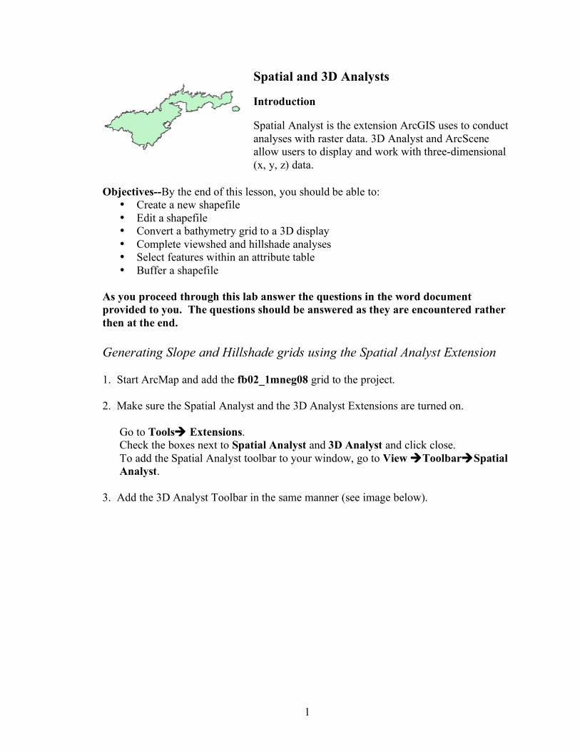
Spatial Analyst is the extension ArcGIS uses to conductanalyses with raster data. 3D Analyst and ArcSceneallow users to display and work with three-dimensional(x, y, z) data.
Citation preview
1
Spatial and 3D Analysts Introduction Spatial Analyst is the extension ArcGIS uses to conduct analyses with raster data. 3D Analyst and ArcScene allow users to display and work with three-dimensional (x, y, z) data.
Objectives--By the end of this lesson, you should be able to:
• Create a new shapefile • Edit a shapefile • Convert a bathymetry grid to a 3D display • Complete viewshed and hillshade analyses • Select features within an attribute table • Buffer a shapefile
As you proceed through this lab answer the questions in the word document provided to you. The questions should be answered as they are encountered rather then at the end. Generating Slope and Hillshade grids using the Spatial Analyst Extension 1. Start ArcMap and add the fb02_1mneg08 grid to the project. 2. Make sure the Spatial Analyst and the 3D Analyst Extensions are turned on.
Go to Tools Extensions. Check the boxes next to Spatial Analyst and 3D Analyst and click close. To add the Spatial Analyst toolbar to your window, go to View ToolbarSpatial Analyst.
3. Add the 3D Analyst Toolbar in the same manner (see image below).
2
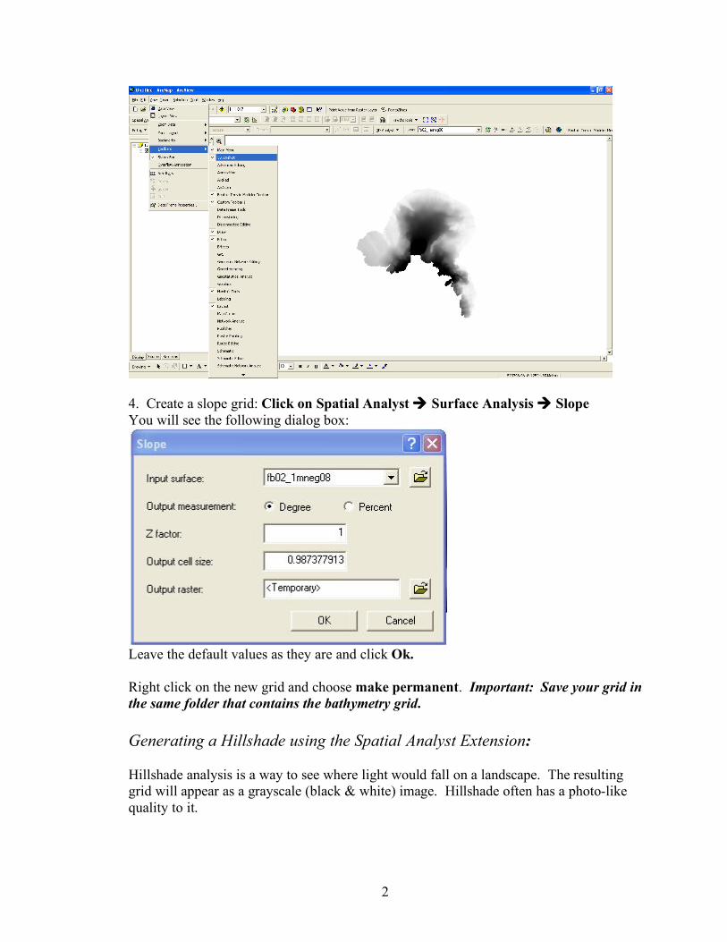
4. Create a slope grid: Click on Spatial Analyst Surface Analysis Slope You will see the following dialog box:
Leave the default values as they are and click Ok. Right click on the new grid and choose make permanent. Important: Save your grid in the same folder that contains the bathymetry grid.
Generating a Hillshade using the Spatial Analyst Extension: Hillshade analysis is a way to see where light would fall on a landscape. The resulting grid will appear as a grayscale (black & white) image. Hillshade often has a photo-like quality to it.
3
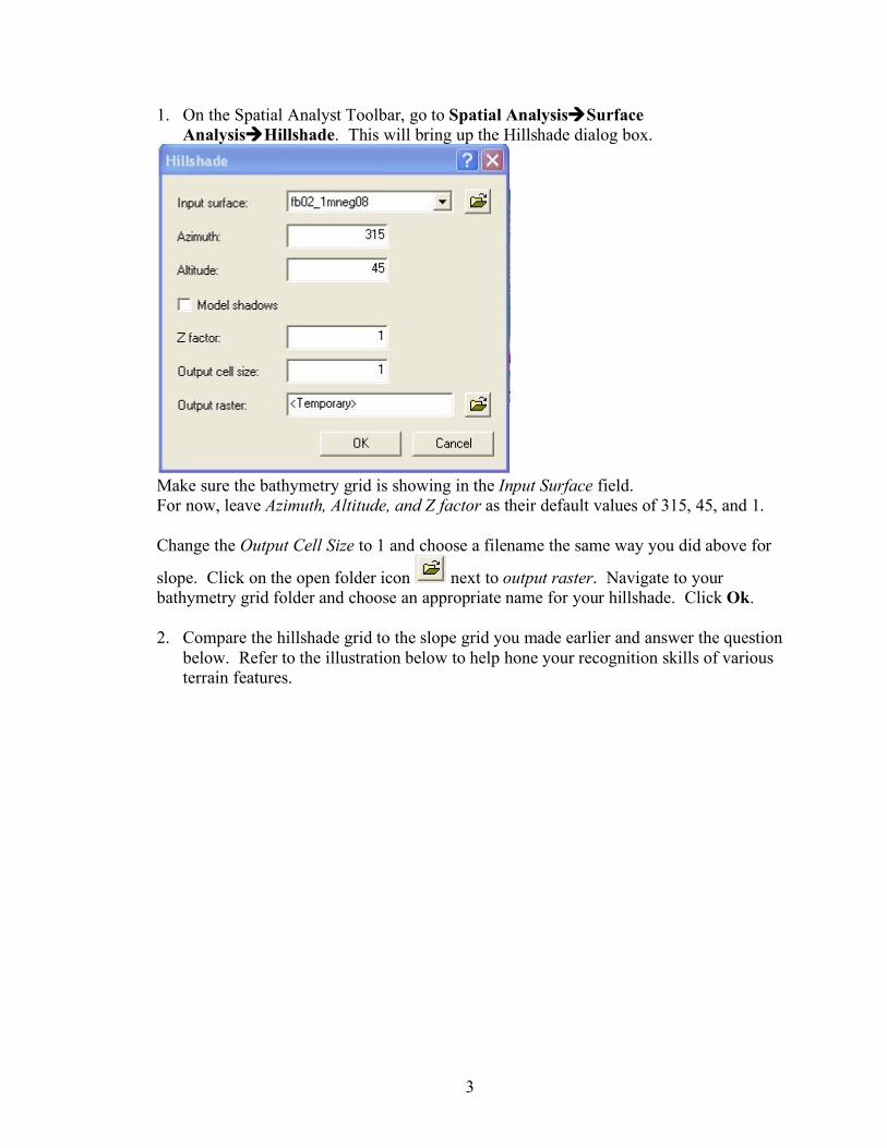
1. On the Spatial Analyst Toolbar, go to Spatial AnalysisSurface AnalysisHillshade. This will bring up the Hillshade dialog box.
Make sure the bathymetry grid is showing in the Input Surface field. For now, leave Azimuth, Altitude, and Z factor as their default values of 315, 45, and 1. Change the Output Cell Size to 1 and choose a filename the same way you did above for
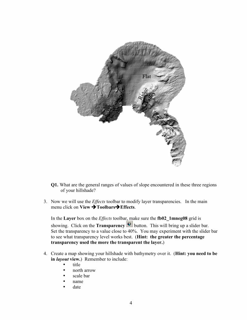
slope. Click on the open folder icon next to output raster. Navigate to your bathymetry grid folder and choose an appropriate name for your hillshade. Click Ok. 2. Compare the hillshade grid to the slope grid you made earlier and answer the question
below. Refer to the illustration below to help hone your recognition skills of various terrain features.
4
Q1. What are the general ranges of values of slope encountered in these three regions
of your hillshade? 3. Now we will use the Effects toolbar to modify layer transparencies. In the main
menu click on View ToolbarsEffects.
In the Layer box on the Effects toolbar, make sure the fb02_1mneg08 grid is showing. Click on the Transparency button. This will bring up a slider bar. Set the transparency to a value close to 40%. You may experiment with the slider bar to see what transparency level works best. (Hint: the greater the percentage transparency used the more the transparent the layer.)
4. Create a map showing your hillshade with bathymetry over it. (Hint: you need to be
in layout view.) Remember to include: • title • north arrow • scale bar • name • date
5
• neatline
Creating a new point shapefile 1. Open ArcCatalog from ArcMap . 2. In ArcCatalog click the name of the folder in which you want to create your shapefile
in the table of contents window (far left window). Now in the ArcCatalog main menu bar, click on FileNew Shapefile. In the Create New Shapefile dialog box, change the name of the file to observer_pts. Make sure that Feature Type is Point and click Ok.
3. Now close ArcCatalog. 4. Go back to ArcMap and add your observer_pts shapefile to your project. Make sure
the Editor toolbar is visible. If not, add it by clicking on ViewToolbar and scrolling to check off the Editor option.
5. On the Editor Toolbar, go to EditorStart Editing. A dialog box will appear with a
statement about your shapefile not being in the same coordinate system as the map. Click Ok.
6. Click on the Digitize Tool . Make sure that the fb02_1mneg08 appears in the dropdown menu. Use the digitize tool to add a point to the observer_pts shapefile by clicking wherever you wish on the map. A highlighted point will appear. Add another five points wherever you would like.
7. Save your edits by going to EditorSave Edits. 8. Stop editing by going to Editor Stop Editing You will use your observer_pts shapefile again later in the lab. 9. Save your project.
Note: Make sure you are saving where you intend! Check the folder in the top of the Save As dialog box. When naming raster files, the name can only be 13 characters long and it is never a good idea to have spaces in a filename.
3D Analyst
1. Launch ArcScene from ArcMap by clicking the ArcScene button in the main menu bar.
2. Add the fb02_1mneg08 and observer_pts files in ArcScene the same way you would add a layer in ArcMap
6
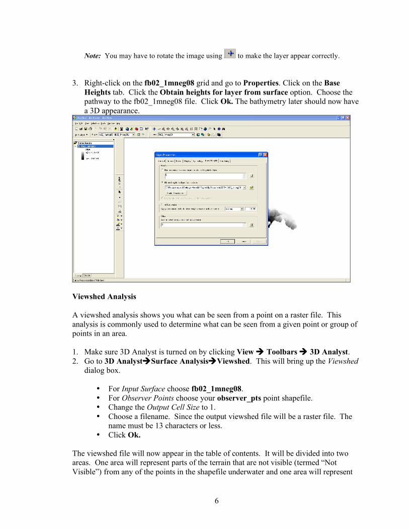
Note: You may have to rotate the image using to make the layer appear correctly. 3. Right-click on the fb02_1mneg08 grid and go to Properties. Click on the Base
Heights tab. Click the Obtain heights for layer from surface option. Choose the pathway to the fb02_1mneg08 file. Click Ok. The bathymetry later should now have a 3D appearance.
Viewshed Analysis A viewshed analysis shows you what can be seen from a point on a raster file. This analysis is commonly used to determine what can be seen from a given point or group of points in an area. 1. Make sure 3D Analyst is turned on by clicking View Toolbars 3D Analyst. 2. Go to 3D AnalystSurface AnalysisViewshed. This will bring up the Viewshed
dialog box.
• For Input Surface choose fb02_1mneg08. • For Observer Points choose your observer_pts point shapefile. • Change the Output Cell Size to 1. • Choose a filename. Since the output viewshed file will be a raster file. The
name must be 13 characters or less. • Click Ok.
The viewshed file will now appear in the table of contents. It will be divided into two areas. One area will represent parts of the terrain that are not visible (termed “Not Visible”) from any of the points in the shapefile underwater and one area will represent
7
parts of the terrain that are visible (termed “Visible”) from any of the points in the shapefile. Using the viewshed grid, answering the following questions: Q2. For what types of applications do you think a viewshed analysis would be useful? Q3. What industries use viewshed analysis? Search the internet to find out. Be sure to
say where you got your information. 3. Now add the hillshade file you created earlier in this lab to your ArcScene project.
Make sure that the viewshed file is first in the layer list (above all other files in the table of contents) and that the hillshade file is second in the layer list.
4. Turn off all other layers (click to uncheck the boxes beside them).
5. Set the Base Heights for the viewshed using the fb02_1mneg08 file.
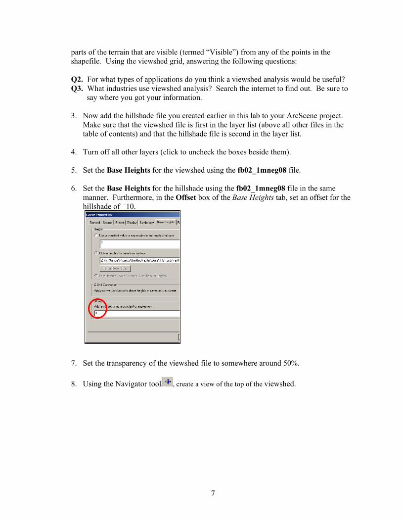
6. Set the Base Heights for the hillshade using the fb02_1mneg08 file in the same manner. Furthermore, in the Offset box of the Base Heights tab, set an offset for the hillshade of –10.
7. Set the transparency of the viewshed file to somewhere around 50%. 8. Using the Navigator tool , create a view of the top of the viewshed.
8
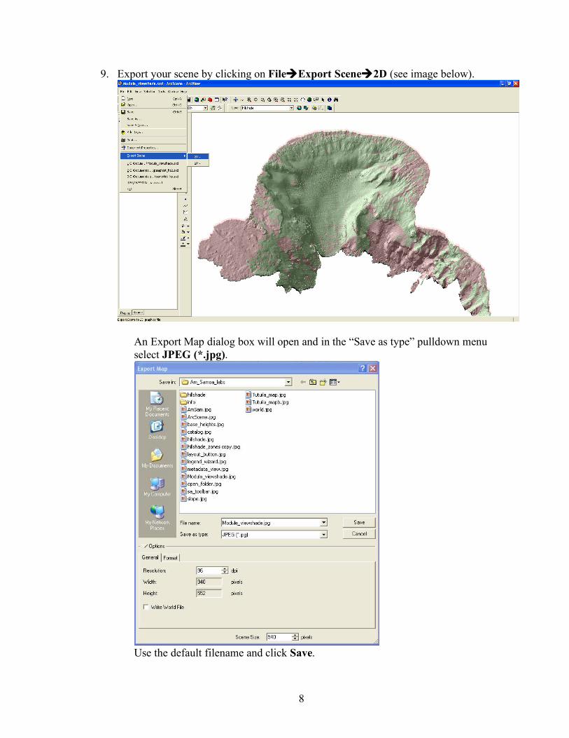
9. Export your scene by clicking on FileExport Scene2D (see image below).
An Export Map dialog box will open and in the “Save as type” pulldown menu select JPEG (*.jpg).
Use the default filename and click Save.
9
10. After saving your viewshed image in ArcScene, exit the ArcScene program by clicking on File Exit.
11. Now open a Microsoft Word Document and Insert your viewshade .jpg file into it.
Save your Word document. MPA Designation Designating Marine Protected Areas (MPAs) can be difficult. It is important that the place chosen to be an MPA protect as many species as possible. Not only must the best location for an MPA be chosen, but the choice must be sensitive to the people who will be affected by a marine reserve in their area. There are two kinds of MPAs in American Samoa: no-take MPAs and MPAs where limited fishing is still allowed. The only no-take MPA in American Samoa is Rose Atoll National Wildlife Sanctuary. Buffering Analysis for an MPA in Fagaitua Bay You should still have your ArcMap project open. 1. Add ftuaneg1m and ftua_ptsfinal, to your project. 2. Right-click on the ftua_ptsfinal shapefile in the table of contents and click zoom to
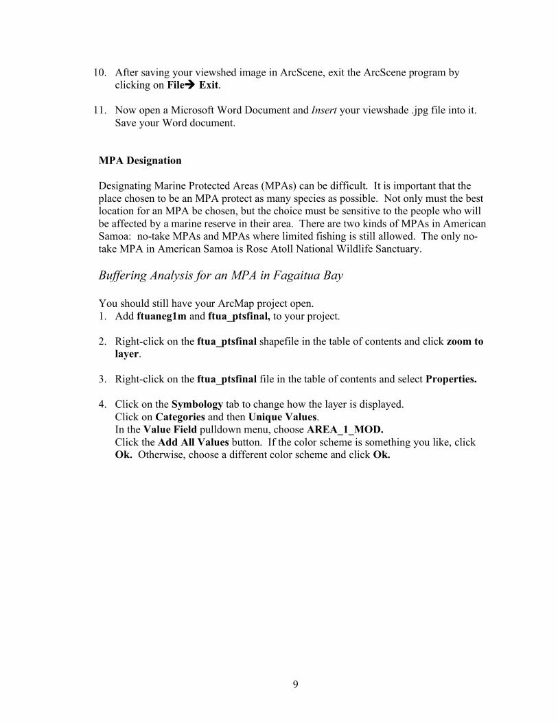
layer. 3. Right-click on the ftua_ptsfinal file in the table of contents and select Properties. 4. Click on the Symbology tab to change how the layer is displayed.
Click on Categories and then Unique Values. In the Value Field pulldown menu, choose AREA_1_MOD. Click the Add All Values button. If the color scheme is something you like, click Ok. Otherwise, choose a different color scheme and click Ok.
10
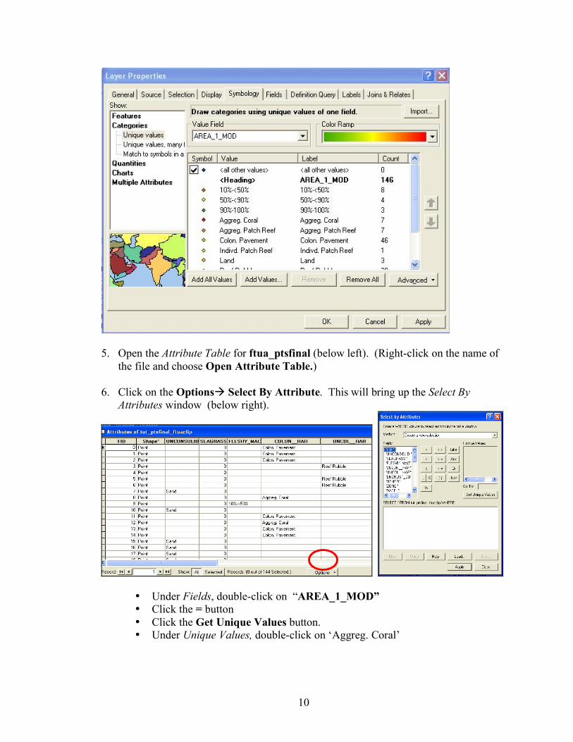
5. Open the Attribute Table for ftua_ptsfinal (below left). (Right-click on the name of the file and choose Open Attribute Table.)
6. Click on the Options Select By Attribute. This will bring up the Select By
Attributes window (below right).
• Under Fields, double-click on “AREA_1_MOD” • Click the = button • Click the Get Unique Values button. • Under Unique Values, double-click on ‘Aggreg. Coral’
11
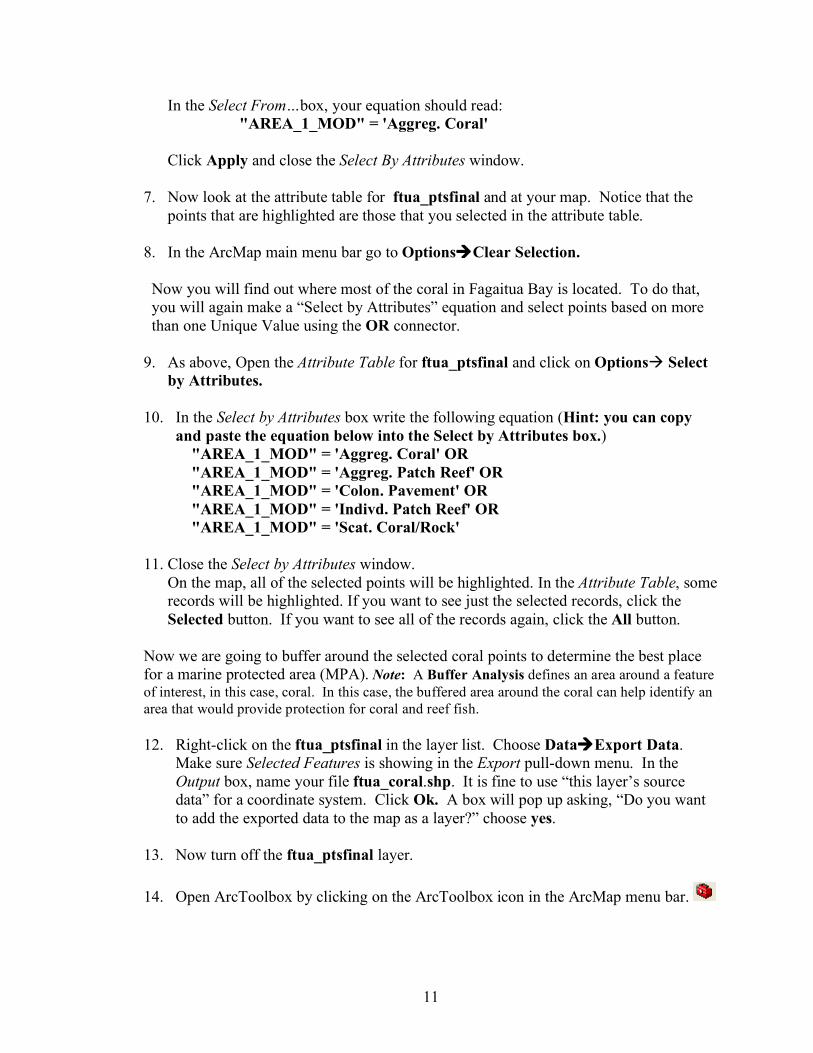
In the Select From…box, your equation should read: "AREA_1_MOD" = 'Aggreg. Coral'
Click Apply and close the Select By Attributes window.
7. Now look at the attribute table for ftua_ptsfinal and at your map. Notice that the points that are highlighted are those that you selected in the attribute table.
8. In the ArcMap main menu bar go to OptionsClear Selection.
Now you will find out where most of the coral in Fagaitua Bay is located. To do that, you will again make a “Select by Attributes” equation and select points based on more than one Unique Value using the OR connector.
9. As above, Open the Attribute Table for ftua_ptsfinal and click on Options Select by Attributes.
10. In the Select by Attributes box write the following equation (Hint: you can copy
and paste the equation below into the Select by Attributes box.) "AREA_1_MOD" = 'Aggreg. Coral' OR "AREA_1_MOD" = 'Aggreg. Patch Reef' OR "AREA_1_MOD" = 'Colon. Pavement' OR "AREA_1_MOD" = 'Indivd. Patch Reef' OR "AREA_1_MOD" = 'Scat. Coral/Rock'
11. Close the Select by Attributes window. On the map, all of the selected points will be highlighted. In the Attribute Table, some records will be highlighted. If you want to see just the selected records, click the Selected button. If you want to see all of the records again, click the All button.
Now we are going to buffer around the selected coral points to determine the best place for a marine protected area (MPA). Note: A Buffer Analysis defines an area around a feature of interest, in this case, coral. In this case, the buffered area around the coral can help identify an area that would provide protection for coral and reef fish.
12. Right-click on the ftua_ptsfinal in the layer list. Choose DataExport Data. Make sure Selected Features is showing in the Export pull-down menu. In the Output box, name your file ftua_coral.shp. It is fine to use “this layer’s source data” for a coordinate system. Click Ok. A box will pop up asking, “Do you want to add the exported data to the map as a layer?” choose yes.
13. Now turn off the ftua_ptsfinal layer. 14. Open ArcToolbox by clicking on the ArcToolbox icon in the ArcMap menu bar.
12
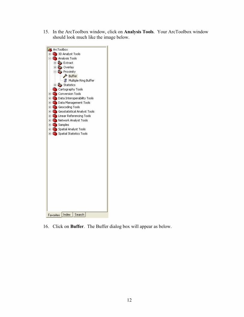
15. In the ArcToolbox window, click on Analysis Tools. Your ArcToolbox window should look much like the image below.
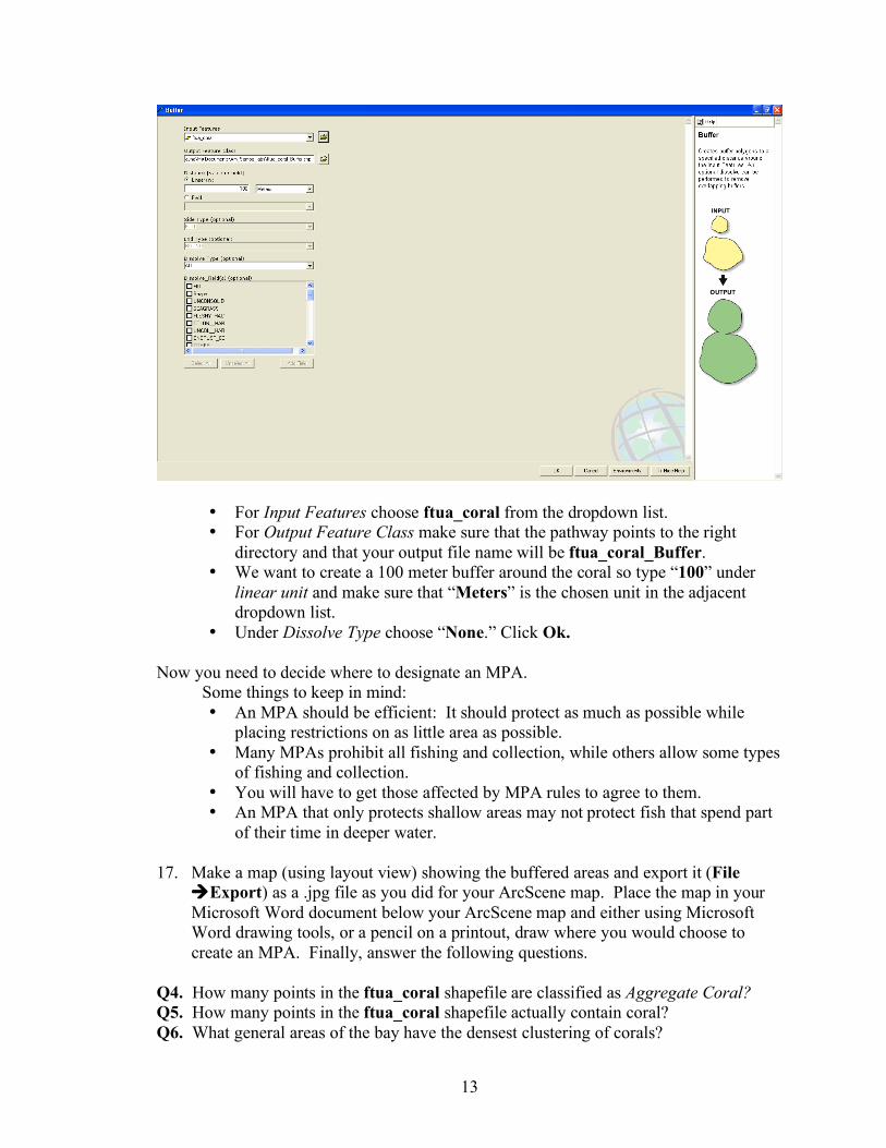
16. Click on Buffer. The Buffer dialog box will appear as below.
13
• For Input Features choose ftua_coral from the dropdown list. • For Output Feature Class make sure that the pathway points to the right
directory and that your output file name will be ftua_coral_Buffer. • We want to create a 100 meter buffer around the coral so type “100” under
linear unit and make sure that “Meters” is the chosen unit in the adjacent dropdown list.
• Under Dissolve Type choose “None.” Click Ok.
Now you need to decide where to designate an MPA. Some things to keep in mind: • An MPA should be efficient: It should protect as much as possible while
placing restrictions on as little area as possible. • Many MPAs prohibit all fishing and collection, while others allow some types
of fishing and collection. • You will have to get those affected by MPA rules to agree to them. • An MPA that only protects shallow areas may not protect fish that spend part
of their time in deeper water.
17. Make a map (using layout view) showing the buffered areas and export it (File Export) as a .jpg file as you did for your ArcScene map. Place the map in your Microsoft Word document below your ArcScene map and either using Microsoft Word drawing tools, or a pencil on a printout, draw where you would choose to create an MPA. Finally, answer the following questions.
Q4. How many points in the ftua_coral shapefile are classified as Aggregate Coral? Q5. How many points in the ftua_coral shapefile actually contain coral? Q6. What general areas of the bay have the densest clustering of corals?