388 QUARTERLY JOURNAL OF ECONOMICSfaculty.wcas.northwestern.edu/~lchrist/finc520/QJE.pdf · MEASURING THE EFFECTS OF MONETARY POLICY: A FACTOR-AUGMENTED VECTOR AUTOREGRESSIVE (FAVAR)

MEASURING THE EFFECTS OF MONETARY POLICY:A FACTOR-AUGMENTED VECTOR AUTOREGRESSIVE

(FAVAR) APPROACH*

BEN S. BERNANKE

JEAN BOIVIN

PIOTR ELIASZ

Structural vector autoregressions (VARs) are widely used to trace out theeffect of monetary policy innovations on the economy. However, the sparse infor-mation sets typically used in these empirical models lead to at least three poten-tial problems with the results. First, to the extent that central banks and theprivate sector have information not reflected in the VAR, the measurement ofpolicy innovations is likely to be contaminated. Second, the choice of a specificdata series to represent a general economic concept such as “real activity” is oftenarbitrary to some degree. Third, impulse responses can be observed only for theincluded variables, which generally constitute only a small subset of the variablesthat the researcher and policy-maker care about. In this paper we investigate onepotential solution to this limited information problem, which combines the stan-dard structural VAR analysis with recent developments in factor analysis forlarge data sets. We find that the information that our factor-augmented VAR(FAVAR) methodology exploits is indeed important to properly identify the mone-tary transmission mechanism. Overall, our results provide a comprehensive andcoherent picture of the effect of monetary policy on the economy.

I. INTRODUCTION

Since Bernanke and Blinder [1992] and Sims [1992], a con-siderable literature has developed that employs vector autore-gression (VAR) methods to attempt to identify and measure theeffects of monetary policy innovations on macroeconomic vari-ables. The key insight of this approach is that identification of theeffects of monetary policy shocks requires only a plausible iden-tification of those shocks (for example, as the unforecasted inno-vation of the federal funds rate in Bernanke and Blinder [1992])and does not require identification of the remainder of the mac-roeconomic model. These methods generally deliver empiricallyplausible assessments of the dynamic responses of key macroeco-nomic variables to monetary policy innovations, and they havebeen widely used both in assessing the empirical fit of structural

* Thanks to Marc Giannoni, Christopher Sims, Mark Watson, Charles White-man, Tao Zha, and two anonymous referees, as well as participants at the 2003NBER Summer Institute for useful comments. Boivin would like to thank theNational Science Foundation for financial support (SES-0214104).

© 2005 by the President and Fellows of Harvard College and the Massachusetts Institute ofTechnology.The Quarterly Journal of Economics, February 2005

387

models (see, for example, Boivin and Giannoni [2003] and Chris-tiano, Eichenbaum, and Evans [forthcoming]) and in policyapplications.

The VAR approach to measuring the effects of monetarypolicy shocks appears to deliver a great deal of useful structuralinformation, especially for such a simple method. Naturally, theapproach does not lack for criticism. For example, researchershave disagreed about the appropriate strategy for identifyingpolicy shocks (Christiano, Eichenbaum, and Evans [2000] surveysome of the alternatives; see also Bernanke and Mihov [1998a]).Alternative identifications of monetary policy innovations can, ofcourse, lead to different inferences about the shape and timing ofthe responses of economic variables. Another issue is that thestandard VAR approach addresses only the effects of unantici-pated changes in monetary policy, not the arguably more impor-tant effects of the systematic portion of monetary policy or thechoice of monetary policy rule [Sims and Zha 1998; Cochrane1996; Bernanke, Gertler, and Watson 1997].

Several criticisms of the VAR approach to monetary policyidentification center around the relatively small amount of infor-mation used by low-dimensional VARs. To conserve degrees offreedom, standard VARs rarely employ more than six to eightvariables.1 This small number of variables is unlikely to span theinformation sets used by actual central banks, which are knownto follow literally hundreds of data series, or by the financialmarket participants and other observers. The sparse informationsets used in typical analyses lead to at least three potential setsof problems with the results. First, to the extent that centralbanks and the private sector have information not reflected in theVAR analysis, the measurement of policy innovations is likely tobe contaminated. A standard illustration of this potential prob-lem, which we explore in this paper, is the Sims [1992] interpre-tation of the so-called “price puzzle,” the conventional finding inthe VAR literature that a contractionary monetary policy shock isfollowed by an increase in the price level, rather than a decreaseas standard economic theory would predict. Sims’s explanationfor the price puzzle is that it is the result of imperfectly control-ling for information that the central bank may have about future

1. Leeper, Sims, and Zha [1996] increase the number of variables included byapplying Bayesian priors, but their VAR systems still typically contain less thantwenty variables.

388 QUARTERLY JOURNAL OF ECONOMICS

inflation. If the Fed systematically tightens policy in anticipationof future inflation, and if these signals of future inflation are notadequately captured by the data series in the VAR, then whatappears to the VAR to be a policy shock may in fact be a responseof the central bank to new information about inflation. Since thepolicy response is likely only to partially offset the inflationarypressure, the finding that a policy tightening is followed by risingprices is explained. Of course, if Sims’s explanation of the pricepuzzle is correct, then all the estimated responses of economicvariables to the monetary policy innovation are incorrect, not justthe price response.

A second problem arising from the use of sparse informationsets in VAR analyses of monetary policy is that it requires takinga stand on specific observable measures corresponding preciselyto some theoretical constructs. The concept of “economic activity,”for example, may not be perfectly represented by industrial pro-duction or real GDP, or any other observable measure.2 Moreover,any observable measure is likely to be contaminated by measure-ment errors.

Finally, impulse responses can be observed only for the in-cluded variables, which generally constitute only a small subsetof the variables that the researcher and policy-makers care about.For example, both for policy analysis and model validation pur-poses, we may be interested in the effects of monetary policyshocks on variables such as total factor productivity, real wages,profits, investment, and many others. Moreover, to assess theeffects of a policy change on an unobserved concept of interestsuch as economic activity, one might wish to document the re-sponses of multiple indicators including, say, employment andsales, to the policy change. Unfortunately, as we have alreadynoted, inclusion of additional variables in standard VARs is se-verely limited by degrees-of-freedom problems.

Is it possible to condition VAR analyses of monetary policy onricher information sets, without giving up the statistical advan-tages of restricting the analysis to a small number of series? Inthis paper we consider one approach to this problem, which com-bines the standard VAR analysis with factor analysis.3 Recent

2. An alternative is to treat economic activity as an unobserved factor withmultiple observable indicators. That is essentially the approach we take in thispaper.

3. Forni, Lippi, and Reichlin [2003] consider a related structural factor modelthat also exploits the information from a large data set. Their approach differs in

389MEASURING THE EFFECTS OF MONETARY POLICY

research in dynamic factor models suggests that the informationfrom a large number of time series can be usefully summarized bya relatively small set of estimated indexes, or factors. For exam-ple, Stock and Watson [2002] develop an approximate dynamicfactor model to summarize the information in large data sets forforecasting purposes.4 They show that forecasts based on thesefactors outperform univariate autoregressions, small vector au-toregressions, and leading indicator models in simulated forecast-ing exercises. Bernanke and Boivin [2003] show that the use ofestimated factors can improve the estimation of the Fed’s policyreaction function.

If a small number of estimated factors effectively summarizelarge amounts of information about the economy, then a naturalsolution to the degrees-of-freedom problem in VAR analyses is toaugment standard VARs with estimated factors. In this paper weconsider the estimation and properties of factor-augmented vec-tor autoregressive models (FAVARs), and then apply these mod-els to the monetary policy issues raised above.

The rest of the paper is organized as follows. Section IIpresents the FAVAR model, motivates it within the context of asimple macroeconomic model, and lays out our estimation ap-proach. We consider both a two-step estimation method, in whichthe factors are estimated by principal components prior to theestimation of the factor-augmented VAR; and a one-step method,which makes use of Bayesian likelihood methods and Gibbs sam-pling to estimate the factors and the dynamics simultaneously.Section III applies the FAVAR methodology to a reexamination ofthe evidence of the effect of monetary policy innovations on keymacroeconomic indicators. In brief, we find that the informationthat the FAVAR methodology extracts is indeed important andleads to broadly plausible estimates for the responses of a widevariety of macroeconomic variables to monetary policy shocks. We

that they identify the common factors as the structural shocks, using long-runrestrictions. In our approach, the latent factors correspond instead to conceptssuch as economic activity. While complementary to theirs, our approach allows 1)a direct mapping with existing VAR results, 2) measurement of the marginalcontribution of the latent factors and 3) a structural interpretation to someequations, such as the policy reaction function.

4. In this paper we follow the Stock and Watson approach to the estimationof factors (which they call “diffusion indexes”). We also employ a likelihood-basedapproach not used by Stock and Watson. Sargent and Sims [1977] first provideda dynamic generalization of classical factor analysis. Forni and Reichlin [1996,1998] and Forni, Hallin, Lippi, and Reichlin [2000] develop a related approach.


also find that the advantages of using the computationally moreburdensome Gibbs sampling procedure instead of the two-stepmethod appear to be modest in this application. Section IV con-cludes. For those readers interested in computational details, anappendix to the working paper version of this article [Bernanke,Boivin, and Eliasz 2004] provides additional information about theapplication of the Gibbs sampling procedure to FAVAR estimation.

II. FAVAR: FRAMEWORK, MOTIVATION, AND ESTIMATION

We begin by laying out a formal framework for factor-augmented VAR analysis. Later in this section we show how thisapproach can be motivated by a simple macroeconomic model anddiscuss approaches to estimation.

II.A. Framework

Let Yt be a M � 1 vector of observable economic variablesassumed to drive the dynamics of the economy. For now, we donot need to specify whether our ultimate interest is in forecastingYt or in uncovering structural relationships among these vari-ables. Following the standard approach in the monetary VARliterature, Yt could contain a policy indicator and observablemeasures of real activity and prices. The conventional approachinvolves estimating a VAR, a structural VAR (SVAR), or othermultivariate time series model using data for Yt alone. However,in many applications, additional economic information, not fullycaptured by Yt, may be relevant to modeling the dynamics ofthese series. Let us suppose that this additional information canbe summarized by a K � 1 vector of unobserved factors, Ft, whereK is “small.” As we illustrate in the next subsection, we mightthink of the unobserved factors as capturing fluctuations in un-observed potential output or reflecting theoretically motivatedconcepts such as “economic activity,” “price pressures,” or “creditconditions” that cannot easily be represented by one or two seriesbut rather are reflected in a wide range of economic variables.

Assume that the joint dynamics of (F�t,Y �t) are given by thefollowing transition equation:

(1) � Ft

Yt� � ��L�� Ft�1

Yt�1� � vt,

where �(L) is a conformable lag polynomial of finite order d, which


may contain a priori restrictions as in the structural VAR litera-ture. The error term vt is mean zero with covariance matrix Q.

Equation (1) is a VAR in (F�t,Y�t). It might be interpretedvariously as an atheoretic forecasting model or as the reducedform of a linear rational-expectations model involving both ob-served and unobserved variables. This system reduces to a stan-dard VAR in Yt if the terms of �(L) that relate Yt to Ft�1 are allzero; otherwise, we will refer to equation (1) as a factor-augmented vector autoregression, or FAVAR. Because the FAVARmodel nests standard VAR analyses, estimation of equation (1)allows for easy comparison with existing VAR results and pro-vides a way of assessing the marginal contribution of the addi-tional information contained in Ft. Note that, if the true systemis a FAVAR, estimation of (1) as a standard VAR system inYt—that is, with the factors omitted—will in general lead tobiased estimates of the VAR coefficients and related quantities ofinterest, such as impulse response coefficients.

Equation (1) cannot be estimated directly because the factorsFt are unobservable. However, as we interpret the factors asrepresenting forces that potentially affect many economic vari-ables, we may hope to infer something about the factors fromobservations on a variety of economic time series. For concrete-ness, suppose that we have available a number of background, or“informational” time series, collectively denoted by the N � 1vector Xt. The number of informational time series N is “large” (inparticular, N may be greater than T, the number of time periods)and will be assumed to be much greater than the number offactors and observed variables in the FAVAR system (K � M ��N). We assume that the informational time series Xt are relatedto the unobservable factors Ft and the observed variables Yt by anobservation equation of the form,

(2) Xt � fFt � yYt � et,

where f is an N � K matrix of factor loadings, y is N � M, andthe N � 1 vector of error terms et are mean zero and will beassumed either normal and uncorrelated or to display a smallamount of cross-correlation, depending on whether estimation isby likelihood methods or principal components (see below).5

5. The principal component estimation allows for some cross-correlation in etthat must vanish as N goes to infinity. See Stock and Watson [2002] for a formaldiscussion of the required restrictions on the cross-correlation of et.


Equation (2) captures the idea that both Yt and Ft, which ingeneral can be correlated, represent common forces that drive thedynamics of Xt. Conditional on Yt, the Xt are thus noisy measuresof the underlying unobserved factors Ft. The implication of equa-tion (2) that Xt depends only on the current and not lagged valuesof the factors is not restrictive in practice, as Ft can be interpretedas including arbitrary lags of the fundamental factors; thus,Stock and Watson [1998] refer to equation (2)—without observ-able factors—as a dynamic factor model.

II.B. Motivating the FAVAR Structure: An Example

A useful application of the FAVAR model, emphasized in thispaper, is to allow researchers to exploit the information from alarge number of indicators in the analysis of empirical macroeco-nomic models. The fact that central banks routinely monitorliterally hundreds of economic variables in the process of policyformulation provides motivation for conditioning any analysis ofmonetary policy on a rich information set [Bernanke and Boivin2003]. In this subsection we use a standard macroeconomicframework both to illustrate why central banks and researchersmay need to consider a long list of information variables and todevelop some implications for the econometric analysis of theeffects of unforecasted changes in monetary policy.

Consider a simple backward-looking model, where the dy-namics of the economy are driven by a handful of macroeconomicforces:6

(3) t � �t�1 � �� yt�1 � yt�1n � � st

(4) yt � yt�1 � ��Rt�1 � t�1� � dt

(5) ytn � �yt�1

n � �t

(6) st � �st�1 � �t.

Equation (3) is an aggregate supply or Phillips curve equationthat relates inflation (t) to lagged inflation (t�1), the laggeddeviations in output from potential ( yt�1 � yt�1

n ), and a cost-push shock (st). Equation (4), an aggregate demand or IS curve,relates output to lagged output, the lagged real interest rate

6. This is a simplified version of the Rudebusch and Svensson [1999] model.The backward-looking specification makes the discussion more transparent. Note,however, that using the results of Svensson and Woodford [2003, 2004], the samepoints could be made in a model embedding forward-looking features.


(Rt�1 � t�1), and a demand shock dt.7 Equations (5) and (6)

specify that potential output and the cost-push shock are first-order autoregressive processes. We take dt, �t, and �t to be meanzero, mutually uncorrelated innovations. Finally, we assume thatthe nominal interest rate Rt is set by the central bank accordingto a simple Taylor rule:

(7) Rt � �t � �� yt � ytn� � εt,

where the central bank responds to current inflation and thedeviations of output from potential. The policy innovation (εt) isassumed to be normally distributed with mean zero and unitvariance. The model is assumed to characterize the business cycledynamics of the economy, to which a large set of N observablemacroeconomic indicators (Xt), are assumed to be related in thefollowing way:

(8) Xt � � ytn st t yt Rt�� et.

As we show next, the model consisting of equations (3)–(8)can be written in vector autoregressive form; however, whetherthe model is properly described by a standard VAR or by aFAVAR depends ultimately on the information structure beingassumed. First, if we rewrite equation (7) in terms of variablesdated t � 1 or earlier, the model can be represented as a con-strained version of equation (1), where

��L� � � � �� 0 0 0 00 � 0 0 00 � � � ��0 0 � ��

�� ,

vt � �0 0 1 00 0 0 10 0 0 11 0 0 0� 1 ��

� � dt

εt

�t

�t

� ,

7. A more natural specification might relate output to the current ex ante realinterest rate rather than the lagged ex post real interest rate. We use thespecification in the text for conformity with the familiar model of Rudebusch andSvensson [1999] and to simplify the calculations. Nothing essential in the subse-quent discussion would be affected if we allowed output to depend on the ex antereal interest rate.


and (F�t Y�t)� � ( ytn st t yt Rt)�. As we will see, the divi-

sion of variables between Ft and Yt depends on which variable(s)are assumed to be directly observed.

If all of the variables in the model are assumed to correspondexactly to empirical measures that are observed both by thecentral bank and the econometrician, then we have that Y�t �( yt

n st t yt Rt)�, Ft equals the null set, and equation (8) isredundant. In this case the model boils down to a restricted VARin Yt. Estimation can proceed by the usual VAR methods. Forexample, following many previous studies, the dynamic effects ofa policy shock, εt, on the economy can be obtained by estimatinga restricted or unrestricted VAR and deriving the implied im-pulse responses.

However, the assumption that both the central bank and theeconometrician observe all the elements of Yt is a strong one.Under alternative, and arguably more realistic, assumptionsabout the information structure, the implied empirical model willgenerally be a FAVAR rather than a standard VAR. Let usconsider some leading cases.

One possibility is that the central bank observes all thevariables in the model, but the econometrician observes only asubset of those variables. For instance the econometrician mightnot observe potential output yt

n and the cost-push shock st di-rectly. In that case, equation (8) can be expressed in the form ofequation (2), with F�t � ( yt

n st)� and Y�t � (t yt Rt)�, and thefull model can be estimated as a FAVAR but not as a standardVAR. In particular, under this information structure, the econo-metrician needs to exploit the information in Xt to properly iden-tify the effects of monetary policy. If the econometrician wereinstead to estimate a standard VAR on the variables Yt that heobserves, he would obtain biased estimates of the policy shockand impulse response functions. As an illustration of the pitfallsof estimating a standard VAR, consider the effects of a negativeproductivity shock in the previous period, �t � 0. This negativeproductivity shock implies a higher nominal interest rate today,through the Taylor rule (7), and higher inflation tomorrow,through the aggregate supply curve (3). By failing to account forthe change in potential output, yt

n, which we have assumed isobserved by the central bank, the researcher would find a spuri-ous association between what appears to be a positive policyshock and an increase in inflation. As we discussed in the Intro-duction, the failure of the econometrician to account for all the


information used by the central bank is one explanation of theprice puzzle.

How can the econometrician avoid this problem? If N weresmall, a simple solution would be to include the indicator vari-ables Xt in the VAR. Such an approach is exemplified by thecommon practice of adding a commodity price index to the VARspecification in order to “fix” the price puzzle. But this practice israther ad hoc, as many variables are likely to contain informationrelevant to the central bank’s decisions; that is, N is likely to belarge. If N is large, adding Xt to an unconstrained VAR withoutexploiting the factor structure would be both inefficient and im-practical (because of degrees-of-freedom problems). In contrast,the FAVAR approach exploits the factor structure, while retain-ing the feature that the investigator may remain agnostic aboutthe structure of the underlying model, in that estimation of theunrestricted form of the FAVAR provides consistent estimates.

The case just considered is based on the assumption that thecentral bank observes the entire relevant information set, includ-ing all the variables entering equations (3)–(7). However, takenliterally, this assumption is inconsistent with the fact that centralbanks monitor a large number of economic indicators. An alter-native, perhaps more plausible, assumption is that the centralbank faces information constraints similar to those of the econo-metrician; that is, the central bank does not directly observepotential output or the cost-push shocks, but exploits the infor-mation from a very large number of macroeconomic indicators.That assumption too would lead to a FAVAR structure, in whichF�t � ( yt

n st)� and Y�t � (t yt Rt)�.8

Rather than develop that case further, however, we notethat, in practice, the information constraints may be even morebinding than we have suggested thus far. For example, one mightargue that even output yt and inflation t are not directly ob-served, either by the central bank or by the econometrician. First,macroeconomic data may be subject to multiple rounds of revi-sions and in any case are never free of measurement error.Second, theoretical concepts do not necessarily align precisely

8. In this case where the central bank does not observe ytn and N is large,

equations (1) and (2) provide a valid approximation to the true dynamics of thesystem. Note, however, that when N is small, the central bank’s estimate of yt

n

independently influences the dynamics of the system, which is not reflected inequations (1) and (2). See Pearlman, Currie, and Levine [1986], Aoki [2003], andSvensson and Woodford [2003a, 2004] for general characterization of a rationalexpectation equilibrium under partial information.


with specific data series. For example, “output” in the theoreticalmodel may correspond more closely to a latent measure of eco-nomic activity, in the spirit of the business cycle analysis of Burnsand Mitchell, than to a specific data series such as real GDP.Similarly, the various biases involved in the measurement ofinflation, such as the inherent difficulty of fully adjusting priceindexes for quality improvement, as well as the availability of avariety of alternative measures of inflation, suggest that exactmeasurement of the “true” rate of inflation is not possible.9 Thesearguments provide some justification for treating output andinflation, as well as concepts like potential output, as unobservedin the empirical analysis. Treating these variables as unobserv-able is one way to acknowledge, at least partly, the real-time dataissues that have been discussed in the literature.10

In short, it may be the case that the most realistic descriptionof the information structure is that the central bank and theeconometrician observe only the policy instrument (the nominalinterest rate), as well as a large set of noisy macroeconomicindicators. In this case, equation (8) can be written in terms ofequation (2), with F�t � (t yt yt�1

n st)� and Yt � Rt. Underthis information structure, the central bank will need to exploitthe information in Xt in formulating monetary policy, a processthat is naturally modeled by the FAVAR structure. Moreover, theeconometrician can use a FAVAR approach to try to describe thecentral bank’s behavior. In the spirit of this last example, ourpreferred empirical specification below will assume that only thepolicy instrument Rt and a large set of macroeconomic indicators,Xt, are observed. However, we also consider specifications thatassume that output and inflation are observable, correspondingto the second case described above. This demonstrates a strengthof the FAVAR approach, that it can accommodate alternativeassumptions about what the central bank and the econometricianobserve, as well as about the information sets that they use.

9. See Boskin [1996] for a discussion of the biases of CPI inflation. See Bils[2004] for a recent investigation of the bias in CPI due to quality growth.

10. Orphanides [2001] argues that assessment of Fed policy depends sensi-tively on whether revised or real-time data are used. Croushore and Evans [1999]do not find this issue to be important for the identification of monetary policyshocks. Bernanke and Boivin [2003] find that in a forecasting context, real-timedata issues were mitigated when the information from a large data set wasexploited. One intuitive explanation is that by considering only the commoncomponents from these measures, the measurement errors are eliminated.


II.C. Estimation

If the structural model laid out in the previous subsectionwere known to characterize precisely the behavior of the econ-omy, the most efficient estimation approach would incorporate allthe restrictions implied by the model’s structure. However, thepotential efficiency gains from imposing strong prior restrictionsmust be weighed against the biases that result if those restric-tions are wrong—a point emphasized by Sims [1980] in the paperin which he introduced VAR analysis to macroeconomics as anantidote to “incredible identifying restrictions.” Fortunately, notall these restrictions are necessary to uncover the effect of aparticular shock, and the FAVAR approach does not impose alimit on the number of potentially useful factors. Following thestandard VAR approach, in our empirical application we focus onspecifications that identify the monetary policy shock while re-maining agnostic about the structure of the rest of the model andthe number of unobservable factors. We stress, however, that noaspect of the FAVAR methodology prevents the imposition ofadditional prior restrictions in estimation.

We consider two approaches to estimating (1)–(2). The firstone is a two-step principal components approach, which providesa nonparametric way of uncovering the common space spannedby the factors of Xt, which we denote by C(Ft,Yt). The second isa single-step Bayesian likelihood approach. These approachesdiffer in various dimensions, and it is not clear a priori that oneshould be favored over the other.

The two-step procedure is analogous to that used in theforecasting exercises of Stock and Watson [2002]. In the first step,the space spanned by the factors is estimated using the first K �M principal components of Xt, which we denote by C(Ft,Yt).

11

Notice that the estimation of the first step does not exploit thefact that Yt is observed. However, as shown in Stock and Watson[2002], when N is large and the number of principal componentsused is at least as large as the true number of factors, theprincipal components consistently recover the space spanned byboth Ft and Yt. Since C(Ft,Yt) corresponds to an arbitrary linearcombination of its arguments, obtaining Ft involves determining

11. A useful feature of this framework, as implemented by an EM algorithm,is that it permits one to deal systematically with data irregularities. In theirapplication, Bernanke and Boivin [2003] estimate factors in cases in which Xtincludes both monthly and quarterly series, series that are introduced midsampleor are discontinued, and series with missing values.


the part of C(Ft,Yt) that is not spanned by Yt.12 In the second

step, the FAVAR, equation (1), is estimated by standard methods,with Ft replaced by Ft. This procedure has the advantages ofbeing computationally simple and easy to implement. As dis-cussed by Stock and Watson [2002], it also imposes few dis-tributional assumptions and allows for some degree of cross-correlation in the idiosyncratic error term et. However, thetwo-step approach implies the presence of “generated regressors”in the second step. To obtain accurate confidence intervals on theimpulse response functions reported below, we implement a boot-strap procedure, based on Kilian [1998], that accounts for theuncertainty in the factor estimation.13

In principle, an alternative is to assume independent normalerrors and to estimate (1) and (2) jointly by maximum likelihood.However, for very large dimensional models of the sort consideredhere, the irregular nature of the likelihood function makes MLEestimation infeasible in practice. In this paper we thus considerthe joint estimation by likelihood-based Gibbs sampling tech-niques, developed by Geman and Geman [1984], Gelman andRubin [1992], and Carter and Kohn [1994], and surveyed in Kimand Nelson [1999]. Their application to large dynamic factormodels is discussed in Eliasz [2002]. Kose, Otrok, and Whiteman[2003, 2004] use similar methodology to study international busi-ness cycles.14

The two methods differ on many important dimensions. Aclear advantage of the two-step approach is computational sim-plicity. Otherwise, it is not clear how the two methods shouldcompare. The two-step approach is semiparametric: it does notimpose the structure of a parametric model with precise distri-butional assumptions in the observation equation (2). Moreover,it does not exploit the structure of the transition equation in the

12. How this is accomplished depends on the specific identifying assumptionused in the second step. We describe below our procedure for the recursiveassumption used in the empirical application.

13. Note that in theory, when N is large relative to T, the uncertainty in thefactor estimates can be ignored; see Bai and Ng [2004].

14. We implement a multimove version of the Gibbs sampler in which factorsare sampled conditional on the most recent draws of the model parameters, andthen the parameters are sampled conditional on the most recent draws of thefactors. As the statistical literature has shown, this Bayesian approach, by ap-proximating marginal posteriors by empirical densities, helps to circumvent thehigh-dimensionality problem of the model. Moreover, the Gibbs-sampling algo-rithm is guaranteed to trace the shape of the joint posterior, even if the posterioris irregular and complicated. See the appendix to the working paper version of thisarticle for more details.


estimation of the factors. The likelihood-based method, on theother hand, is fully parametric. The methods will thus implydifferent biases and variances, which will depend on how wellspecified the model is. By comparing the results from the twomethods, we may be able to assess whether the advantages ofjointly estimating the model are worth the computational costs.

II.D. Identification

There are two different sets of restrictions that need to beimposed on the system (1)–(2). The first is a minimum set ofnormalization restrictions on the observation equation (2) thatare needed to be able to estimate the model at all. This normal-ization is an issue separate from the identification of the policyshock per se, which requires imposing further restriction on thetransition equation (1), and potentially on the observation equa-tion (2) as well.

As it is written, model (1)–(2) is econometrically unidentifiedand cannot be estimated. Since we leave the VAR dynamics inequation (1) unrestricted, identification proceeds by imposingrestrictions on factors and their coefficients in equation (2). As-sume that f and Ft are a solution to the estimation problem. Wecould define f � f H and Ft � H�1Ft, where H is a K � Knonsingular matrix, which would also satisfy equation (2). As aresult, observing Xt cannot help distinguishing between thesetwo solutions.15 A normalization must then be imposed. Note,however, that since Ft covers the same space as Ft, such normal-ization does not affect the information content of the estimatedfactors.

In two-step estimation by principal components, where weare not explicitly imposing Yt as being observable in the first step,we use the standard normalization implicit in the principal com-ponents, that is, we take C�C/T � I, where C� � [C(F1,Y1), . . . ,C(FT,YT)]. This implies that C � �T Z, where the Z are theeigenvectors corresponding to the K largest eigenvalues of XX�,sorted in descending order. In the “one-step” (joint estimation)likelihood method, this approach needs to be modified to accountfor the fact that Yt enters the observation equation. Sufficient

15. In the case where Ft is a scalar, this is simply saying that its scale is notidentified, and thus needs to be normalized. This is what Anderson [1984, p. 552]refers to as the “fundamental indeterminacy” of this model.


conditions are to set the upper K � K block of f to an identitymatrix and the upper K � M block of y to zero.16

The identification of the structural shocks in the transitionequation requires further restrictions. In the empirical applica-tion we consider below, and consistent with the example struc-tural model of subsection II.B, we will assume a recursive struc-ture where all the factors entering (1) respond with a lag tochange in the monetary policy instrument, ordered last in Yt. Inthat case, we do not need to identify the factors separately, butonly the space spanned by the latent factors Ft. In terms of themacroeconomic model discussed above, that means that we onlyneed four distinct linear combinations of t, yt, yt

n, and st, but wedo not need to identify each of these latent variables individually.As a result, no further restrictions are required in the observationequation (2), and the identification of the policy shock can beachieved in (1) as if it were a standard VAR.

Importantly, other identification schemes (e.g., long-run re-strictions as in Blanchard and Quah [1989] or structural VARprocedures as in Bernanke and Mihov [1998a]) can be imple-mented in the FAVAR framework. These would typically require,however, that some of the factors be identified as specific eco-nomic concepts. For instance, implementing a long-run restric-tion that stipulates that monetary policy shocks do not have along-run effect on the output gap would require identifying ( yt �yt

n) separately from the other factors. But this can easily beachieved by imposing restrictions on the factor loading matrix (inthe likelihood setting) or extracting principal components fromblocks of data corresponding to different dimensions of the econ-omy. For instance, real-activity measures (e.g., components ofindustrial production, employment, and consumption) could beassumed to load solely on (yt � yt

n). The same idea could be appliedmore generally to implement alternative identification schemes.

One caveat is that the use of the Gibbs sampling methodologymay impose significant computational costs when complex iden-tification schemes are employed. For example, if we impose re-strictions that overidentify the transition equation, we need toperform numerical optimization at each step of the Gibbs sam-

16. In the joint estimation case, the normalization needs to rule out linearcombinations of the form F*t � AFt � BYt, where A is K � K and nonsingular,and B is K � M. Substituting for Ft in (2), we obtain Xt � fA�1F*t � (y �fA�1B)Yt � et. To induce F*t � Ft, that is A � IK and B � 0K�M, it suffices toimpose restrictions such as those specified in the text.


pling procedure. This may easily become excessively time con-suming. In part for computational simplicity we use a simplerecursive ordering in our empirical application below.

III. APPLICATION: THE DYNAMIC EFFECTS OF MONETARY POLICY

As discussed in the Introduction, an extensive literature hasemployed VARs to study the dynamic effects of innovations tomonetary policy on a variety of economic variables. A variety ofidentification schemes have been employed, including simple re-cursive frameworks, “contemporaneous” restrictions (on the ma-trix relating structural shocks to VAR disturbances), “long-run”restrictions (on the shape of impulse responses at long horizons),and mixtures of contemporaneous and long-run restrictions.17

Alternative estimation procedures have been employed as well,including Bayesian approaches [Leeper, Sims, and Zha 1996].However, the basic idea in virtually all cases is to identify“shocks” to monetary policy with the estimated innovations to avariable or linear combination of variables in the VAR. Once thisidentification is made, estimating dynamic responses to monetarypolicy innovations (as measured by impulse response functions) isstraightforward.

The fact that this simple method typically gives plausible anduseful results with minimal identifying assumptions accounts forits extensive application, both by academic researchers and bypractitioners in central banks. Nevertheless, a number of cri-tiques of the approach have been made (see, for example, Rude-busch [1998]). The FAVAR approach described in the previoussection can address some of these problems.

Section II emphasized three reasons why the usual VARanalysis might be inappropriate under some realistic informationstructures. First, small-scale VARs are unlikely to cover theinformation set of policy-makers, which is likely to lead to biased

17. Recursive frameworks are employed, inter alia, in Bernanke and Blinder[1992], Sims [1992], Strongin [1995], and Christiano, Eichenbaum, and Evans[2000]. Examples of papers with contemporaneous, nonrecursive restrictions areGordon and Leeper [1994], Leeper, Sims, and Zha [1996], and Bernanke andMihov [1998a]. Long-run restrictions are employed by Lastrapes and Selgin[1995] and Gerlach and Smets [1995]. Gali [1992] and Bernanke and Mihov[1998b] use a mixture of contemporaneous and long-run restrictions. Faust andLeeper [1997] and Pagan and Robertson [1998] point out some dangers of relyingtoo heavily on long-run restrictions for identification in VARs.


inference. Second, the choice of a specific data series to representa general economic concept (e.g., industrial production for “eco-nomic activity,” the consumer price index for “the price level”) isoften arbitrary to some degree; measurement errors and revisionspose additional problems for linking theoretical concepts to spe-cific data series. Finally, even if monetary policy shocks areproperly identified, standard VAR analyses have the shortcomingthat the dynamic responses of only those few variables includedin the VAR can be estimated. For purposes both of policy analysisand model validation, it is often useful to know the effects ofmonetary policy on a lengthy list of variables.18

The FAVAR framework is well-suited to investigate the em-pirical importance of these issues. First, since the system (1)–(2)nests the standard VAR specification, we can determine directlywhether the additional information conveyed by the unobservedfactors is relevant or not. Second, because it allows for the use ofmultiple indicators of underlying economic concepts, the FAVARapproach can be implemented without having to assume thatconcepts such as “real activity” or “price pressures” are observed.Finally, this methodology can be used to draw out the dynamicresponses of not only the “main” variables Yt but of any seriescontained in Xt. Hence the “reasonableness” of a particular iden-tification can be checked against the behavior of many variables,not just three or four.

III.A. Empirical Implementation

We apply both the two-step and “one-step” (joint estimation)methodologies to the estimation of monetary FAVARs. In ourapplications, Xt consists of a balanced panel of 120 monthlymacroeconomic time series (updates of series used in Stock andWatson [1998, 1999]).19 These series are initially transformed to

18. One approach to this problem is to assume no feedback from variablesoutside the basic VAR, that is, a block-recursive structure with the base VARordered first (see Bernanke and Gertler [1995]). However, the no-feedback as-sumption is dubious in many cases.

19. The choice of which data to include in Xt might not be innocuous. Whilein theory more data are always better (see Stock and Watson [2002]), in practicethat often means more of the same type of data, like for instance, more measuresof real activity. Boivin and Ng [forthcoming] provide examples, where simplyadding more data has perverse effects. They also investigate these issues in thecontext of a forecasting exercise based on a data set very similar to ours. They findthat it is possible to forecast equally well, and perhaps marginally better, byestimating factors from as few as 40 prescreened series. The prescreening is,however, largely ad hoc, and the cost from using all series, if any, is marginal.


induce stationarity. The description of the series in the data setand their transformation is described in Appendix 1. The dataspan the period from January 1959 through August 2001.

In subsection II.B we described alternative specificationsarising from alternative assumptions about the informationstructure. For reasons we gave, our preferred specification treatsthe Fed’s policy instrument Rt (in our application the federalfunds rate) as observable and other variables, including outputand inflation, as unobservable. In this case, Rt is the only variableincluded in the vector of observable variables, Yt. In what follows,we compare this preferred specification with alternative VAR andFAVAR specifications corresponding to alternative informationstructures. In each specification, the monetary policy shock isidentified in the standard recursive manner, that is by orderingthe federal funds rate last and treating its innovations as thepolicy shocks.

The recursive ordering imposes the identifying assumptionthat the unobserved factors do not respond to monetary policyinnovations within the period (here, a month). However, we neednot impose that assumption on the idiosyncratic components ofthe information variables. In particular, we define two categoriesof information variables: “slow-moving” and “fast-moving.” Slow-moving variables (think of wages or spending) are assumed not torespond contemporaneously to unanticipated changes in mone-tary policy. In contrast, fast-moving variables (think of assetprices) are allowed to respond contemporaneously to policyshocks. The classification of variables into the two categories isprovided in Appendix 1. As discussed above, the joint likelihoodestimation only requires that the first K variables in the data setare selected from the set of slow-moving variables and that therecursive structure is imposed in the transition equation.

For the two-step estimation approach, as we explained above,we rely in the first step on the fact that when N is large, theprincipal components estimated from the entire data set,C(Ft,Yt), consistently recover K � M independent, but arbitrary,linear combinations of Ft and Yt. Since Yt is not explicitly im-posed as a common component in the first step, any of the linearcombinations underlying C(Ft,Yt) could involve the Fed’s policyinstrument, Rt, which is included in Yt in all the specifications weconsider. It would thus not be valid to simply estimate a VAR in


C(Ft,Yt) and Yt, and identify the policy shock recursively. In-stead, the direct dependence of C(Ft,Yt) on Rt must first beremoved. If linear combinations implicit in C(Ft,Yt) wereknown, this would involve subtracting Rt times the associatedcoefficient from each of the elements of C(Ft,Yt).

20 Giventhat they are unknown, our strategy is to estimate their coeffi-cients through a multiple regression of the form C(Ft,Yt) �bC*C*(Ft) � bRRt � et, where C*(Ft) is an estimate of all thecommon components other than Rt. One way to obtain C*(Ft)is to extract principal components from the subset of slow-movingvariables, which by assumption are not affected contemporane-ously by Rt. Ft is then constructed as C(Ft,Yt) � bRRt and a VARin Ft and Yt is estimated and identified recursively, with Rtordered last.

III.B. Empirical ResultsWe begin by comparing the results from a standard three-

variable VAR—based on industrial production, CPI, and the fed-eral funds rate—with two FAVAR specifications: 1) our preferredFAVAR specification, where only the federal funds is assumed tobe observed, and 2) the three-variable VAR expanded with oneunobservable factor. The latter FAVAR model nests the VAR andthus allows us to isolate the marginal contribution of the addi-tional information. Since the economy might have other unmod-eled dimensions, we check below the robustness of the results toan alternative number of factors. We use thirteen lags, but em-ploying seven lags led to very similar results. We standardize themonetary shock to correspond to a 25-basis-point innovation inthe federal funds rate. Note that the figures report impulse re-sponses, in standard deviation units.

Figure I displays the resulting impulse response functions,obtained from the two-step estimation. There is a strong pricepuzzle in the VAR specification and the response of industrialproduction is very persistent, inconsistent with long-run moneyneutrality. Adding one factor to standard VAR changes the re-sponses dramatically.21 The price puzzle is considerably reduced,

20. Note that the other common factors will in general be correlated with Rt.For instance, in terms of our illustration in Section II, the policy instrument Rtis correlated with the other variable of the model, i.e., (t yt yt�1

n st)�, whichcould all be unobserved. As a result, the residuals from a regression of C(Ft,Yt)on Rt would not be appropriate.

21. In this case, adding one factor appears to be all that is needed. Adding upto seven factors did not change the results.


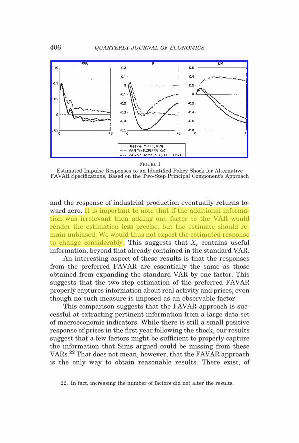
and the response of industrial production eventually returns to-ward zero. It is important to note that if the additional informa-tion was irrelevant then adding one factor to the VAR wouldrender the estimation less precise, but the estimate should re-main unbiased. We would thus not expect the estimated responseto change considerably. This suggests that Xt contains usefulinformation, beyond that already contained in the standard VAR.

An interesting aspect of these results is that the responsesfrom the preferred FAVAR are essentially the same as thoseobtained from expanding the standard VAR by one factor. Thissuggests that the two-step estimation of the preferred FAVARproperly captures information about real activity and prices, eventhough no such measure is imposed as an observable factor.

This comparison suggests that the FAVAR approach is suc-cessful at extracting pertinent information from a large data setof macroeconomic indicators. While there is still a small positiveresponse of prices in the first year following the shock, our resultssuggest that a few factors might be sufficient to properly capturethe information that Sims argued could be missing from theseVARs.22 That does not mean, however, that the FAVAR approachis the only way to obtain reasonable results. There exist, of

22. In fact, increasing the number of factors did not alter the results.

FIGURE IEstimated Impulse Responses to an Identified Policy Shock for Alternative

FAVAR Specifications, Based on the Two-Step Principal Component’s Approach


http://www.mitpressjournals.org/action/showImage?doi=10.1162/qjec.2005.120.1.387&iName=master.img-000.png&w=296&h=145

IBM USER

Highlight

course, other VAR specifications and identification schemes thatcould lead to reasonable results over some periods. For example,some authors have “improved” their results by adding variablessuch as an index of commodity prices to the VAR.23 But unlessthese variables are part of the theoretical model the researcherhas in mind, it is not clear on what grounds they are selected,other than the fact that they “work.” The advantage of our ap-proach is to put discipline on the process, by explicitly recognizingin the econometric model the scope for additional information. Asa result, the fact that adding the commodity price index—or anyother variables—fixes or not the price puzzle is not directly rele-vant to our comparison.

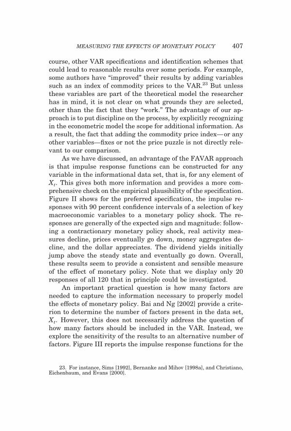
As we have discussed, an advantage of the FAVAR approachis that impulse response functions can be constructed for anyvariable in the informational data set, that is, for any element ofXt. This gives both more information and provides a more com-prehensive check on the empirical plausibility of the specification.Figure II shows for the preferred specification, the impulse re-sponses with 90 percent confidence intervals of a selection of keymacroeconomic variables to a monetary policy shock. The re-sponses are generally of the expected sign and magnitude: follow-ing a contractionary monetary policy shock, real activity mea-sures decline, prices eventually go down, money aggregates de-cline, and the dollar appreciates. The dividend yields initiallyjump above the steady state and eventually go down. Overall,these results seem to provide a consistent and sensible measureof the effect of monetary policy. Note that we display only 20responses of all 120 that in principle could be investigated.

An important practical question is how many factors areneeded to capture the information necessary to properly modelthe effects of monetary policy. Bai and Ng [2002] provide a crite-rion to determine the number of factors present in the data set,Xt. However, this does not necessarily address the question ofhow many factors should be included in the VAR. Instead, weexplore the sensitivity of the results to an alternative number offactors. Figure III reports the impulse response functions for the

23. For instance, Sims [1992], Bernanke and Mihov [1998a], and Christiano,Eichenbaum, and Evans [2000].


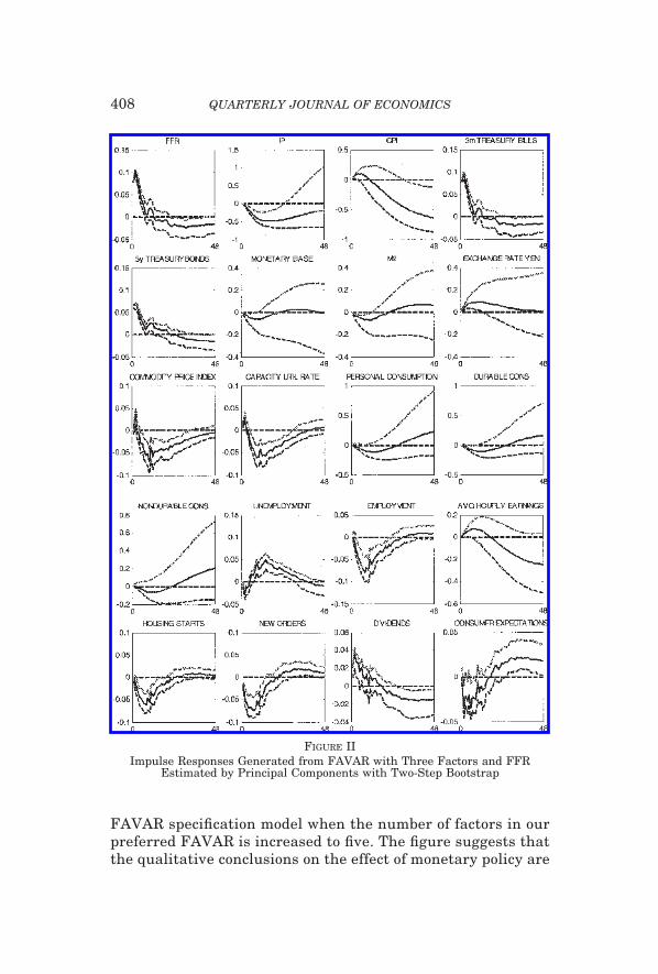
FAVAR specification model when the number of factors in ourpreferred FAVAR is increased to five. The figure suggests thatthe qualitative conclusions on the effect of monetary policy are

FIGURE IIImpulse Responses Generated from FAVAR with Three Factors and FFR

Estimated by Principal Components with Two-Step Bootstrap



not altered by the use of five factors. Further increases in thenumber of factors did not change qualitative nature of ourresults.

FIGURE IIIImpulse Responses Generated from FAVAR with Five Factors and FFR

Estimated by Principal Components with Two-Step Bootstrap



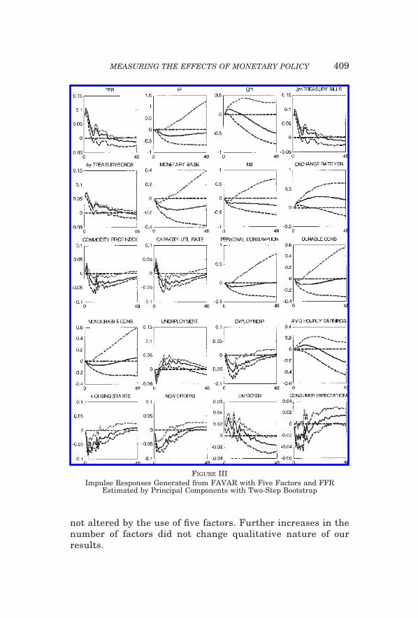
Figures IV and V report the same results as Figures II andIII, but from the likelihood-based estimation. The estimationwas implemented with 10,000 iterations of the Gibbs sampling

FIGURE IVImpulse Responses Generated from FAVAR with Three Factors and FFR

Estimated by Gibbs Sampling



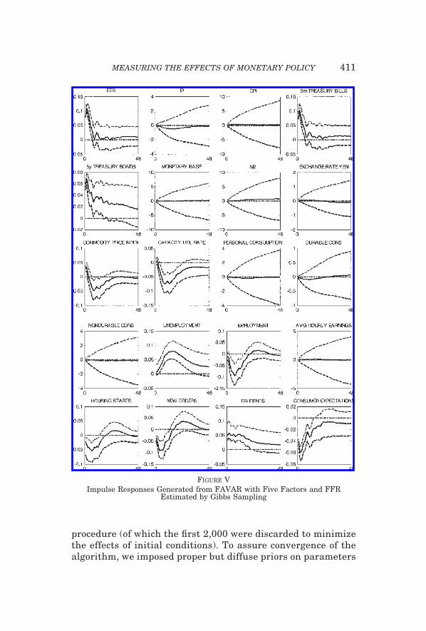
procedure (of which the first 2,000 were discarded to minimizethe effects of initial conditions). To assure convergence of thealgorithm, we imposed proper but diffuse priors on parameters

FIGURE VImpulse Responses Generated from FAVAR with Five Factors and FFR

Estimated by Gibbs Sampling



of the observation and the VAR equations.24 There seemed tobe no problems achieving convergence, and alternative startingvalues or the use of 20,000 iterations gave essentially the sameresults.

In this case, while responses of prices and money aggregatesare very imprecisely estimated, overall the point estimates of theresponses are quite similar to those reported for the two-stepapproach. We find it remarkable that the two rather differentmethods, producing distinct factor estimates, give qualitativelysimilar results. On the other hand, the degree of uncertaintyabout the estimates implied by the two methods is quite different.Increasing the number of factors does not appear to improve theresults. This might suggest that the likelihood-based estimation,being fully parametric, as detailed in subsection II.C, suffers fromthe additional structure it imposes and produces factors that donot successfully capture information about real-activity andprices. This intuition is strengthened by the fact that the Gibbsestimation of FAVAR with CPI and industrial production as extraobservable factors delivers results (not reported in the paper)much more in line with those obtained by a two-step procedure.

To assess whether differences between results are due todifferences in the information content of the factor estimates, weestimated factors from both approaches using the same identifi-cation. This was accomplished by setting loadings on Y to zero inthe observation equation for the likelihood-based estimation and,in the two-step approach, by not removing the direct dependenceof the principal components on the federal funds rate (see sub-section III.A). These are the alternative ways of partialling outthe effects of the federal funds rate from the estimated factors. Asit turns out, the two sets of factors generated in this way aresignificantly different. The factors estimated by principal compo-nents fully explain the variance of likelihood-estimated factors,but the opposite is not true. Moreover, the principal componentfactors have greater short-run variation. We interpret these find-ings as evidence that the differences in identification are not thesole source of the differences in results. Since it is the likelihood

24. We have also experimented with flat priors which yielded the samequalitative results. Prior specifications are discussed in the appendix to theworking paper version of this article.


method that imposes additional structure on the model, we mayexpect PC factors to carry more information.25

Other than impulse response functions, another exercise typ-ically performed in the standard VAR context is variance decom-position. This consists of determining the fraction of the forecast-ing error of a variable, at a given horizon, that is attributable toa particular shock. Variance decomposition results follow imme-diately from the coefficients of the MA representation of the VARsystem and the variance of the structural shocks. For instance thefraction variance of (Yt�k � Yt�k) due to the monetary policyshock could be expressed as

var �Yt�k � Yt�k�t�εtMP�

var �Yt�k � Yt�k�t�.

A standard result of the VAR literature is that the monetarypolicy shock explains a relatively small fraction of the forecasterror of real activity measures or inflation.

Table I reports the results for the same twenty macroeco-nomic indicators analyzed in the previous figures. These arebased on the two-step estimation of the benchmark specification.The first column reports the contribution of the monetary policyshock to the variance of the forecast error at the 60-month hori-zon. The second column contains the R2 of the common compo-nent for each of these variables.26

Apart from the interest rates, the contribution of the policyshock ranges between 0 and 10.3 percent. This suggests a rela-tively small effect of the monetary policy shock. In particular, thepolicy shock explains 10.3 percent, 10.0 percent, and 8.6 percentof unemployment, capacity utilization and new orders, respec-tively, and 5.4 percent of industrial production. Looking at the R2

of the common component, we note two points. First, the factorsexplain a sizable fraction of these variables, in particular for someof the most prominent macroeconomic indicators: industrial pro-duction (70.7 percent), employment (72.3 percent), unemploy-ment (81.6 percent), and the consumer price index (86.9 percent).This confirms that the FAVAR framework, estimated by the

25. This is confirmed in a forecasting exercise (not reported), in which weevaluated predictive power of the two sets of factors for CPI, industrial produc-tion, and unemployment. As expected, principal components perform moderatelybetter, particularly when forecasting at longer horizons.

26. Note that since FFR is assumed to be an observed factor, the correspond-ing R2 is one by construction.


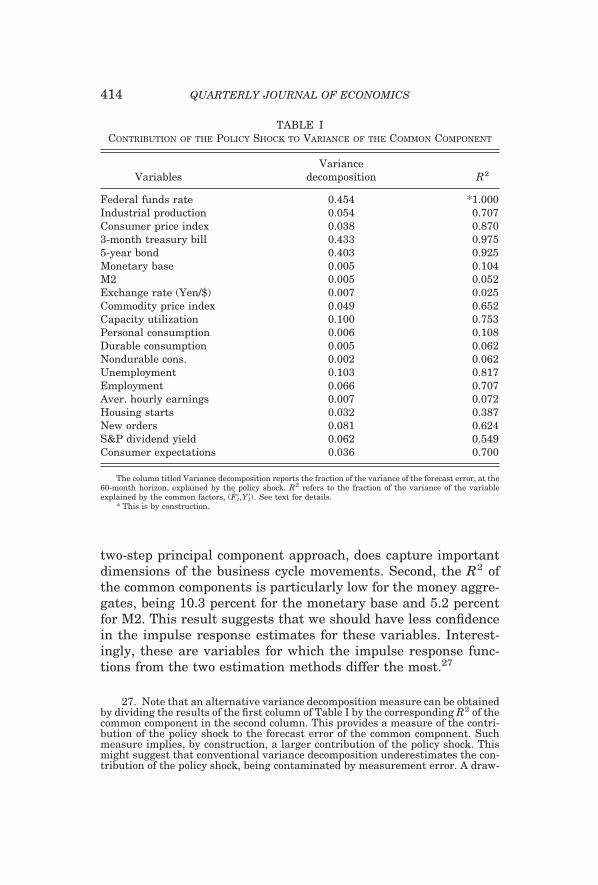
two-step principal component approach, does capture importantdimensions of the business cycle movements. Second, the R2 ofthe common components is particularly low for the money aggre-gates, being 10.3 percent for the monetary base and 5.2 percentfor M2. This result suggests that we should have less confidencein the impulse response estimates for these variables. Interest-ingly, these are variables for which the impulse response func-tions from the two estimation methods differ the most.27

27. Note that an alternative variance decomposition measure can be obtainedby dividing the results of the first column of Table I by the corresponding R2 of thecommon component in the second column. This provides a measure of the contri-bution of the policy shock to the forecast error of the common component. Suchmeasure implies, by construction, a larger contribution of the policy shock. Thismight suggest that conventional variance decomposition underestimates the con-tribution of the policy shock, being contaminated by measurement error. A draw-

TABLE ICONTRIBUTION OF THE POLICY SHOCK TO VARIANCE OF THE COMMON COMPONENT

VariablesVariance

decomposition R2

Federal funds rate 0.454 *1.000Industrial production 0.054 0.707Consumer price index 0.038 0.8703-month treasury bill 0.433 0.9755-year bond 0.403 0.925Monetary base 0.005 0.104M2 0.005 0.052Exchange rate (Yen/$) 0.007 0.025Commodity price index 0.049 0.652Capacity utilization 0.100 0.753Personal consumption 0.006 0.108Durable consumption 0.005 0.062Nondurable cons. 0.002 0.062Unemployment 0.103 0.817Employment 0.066 0.707Aver. hourly earnings 0.007 0.072Housing starts 0.032 0.387New orders 0.081 0.624S&P dividend yield 0.062 0.549Consumer expectations 0.036 0.700

The column titled Variance decomposition reports the fraction of the variance of the forecast error, at the60-month horizon, explained by the policy shock. R2 refers to the fraction of the variance of the variableexplained by the common factors, (F�t,Y�t). See text for details.

* This is by construction.


IV. CONCLUSION

This paper has introduced a method for incorporating a broadrange of conditioning information, summarized by a small num-ber of factors, in otherwise standard VAR analyses. We haveshown how to identify and estimate a factor-augmented vectorautoregression, or FAVAR, by both a two-step method based onestimation of principal components and a more computationallydemanding, Bayesian method based on Gibbs sampling. Anotherkey advantage of the FAVAR approach is that it permits us toobtain the responses of a large set of variables to monetary policyinnovations, which provides both a more comprehensive pictureof the effects of policy innovations as well as a more completecheck of the empirical plausibility of the underlying specification.

In our monetary application of FAVAR methods, we find thatoverall the two methods produce qualitatively similar results,although the two-step approach tends to produce more plausibleresponses, and does so without our having to take a stand onspecific measures of real activity or prices. Moreover, the resultsprovide some support for the view that the “price puzzle” resultsfrom the exclusion of conditioning information. The conditioninginformation also leads to reasonable responses of money aggre-gates. These results thus suggest that there is a scope to exploitmore information in empirical macroeconomic modeling.

Future work should investigate more fully the properties ofFAVARs, alternative estimation methods and alternative identi-fication schemes. In particular, further comparison of the estima-tion methods based on principal components and on Gibbs sam-pling is likely to be worthwhile. Another interesting direction is totry to interpret the estimated factors more explicitly. For exam-ple, according to the original Sims [1992] hypothesis, if the addi-tion of factors mitigates the price puzzle, then the factors shouldcontain information about future inflation not otherwise capturedin the VAR. The marginal contribution of the estimated factorsfor forecasting inflation can be checked directly.28

back of this alternative measure, however, is that it is model dependent, in thesense that different factor estimates, or different numbers of them, will implydifferent results.

28. Stock and Watson [1999] and Bernanke and Boivin [2003] have shownthat, generally, factor methods are useful for forecasting inflation.


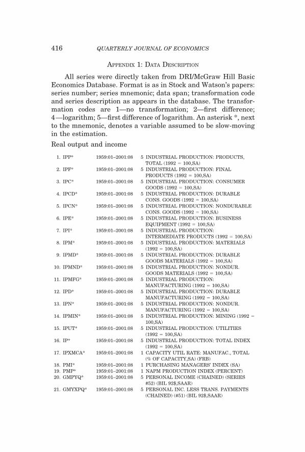
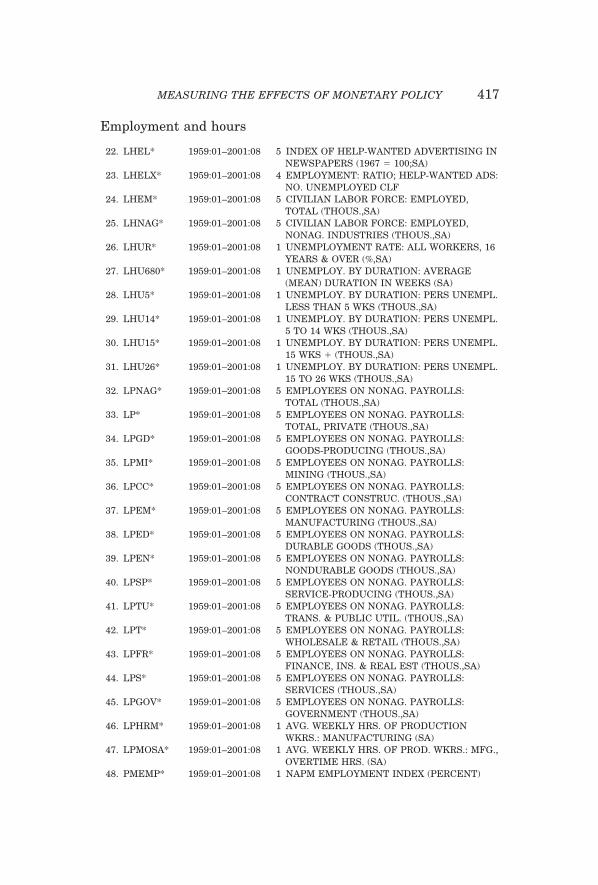
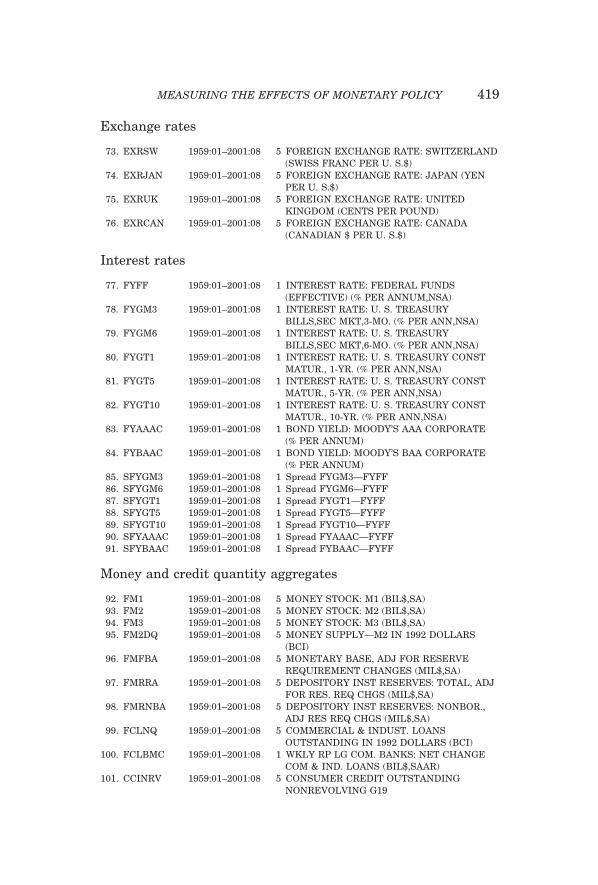
APPENDIX 1: DATA DESCRIPTION

All series were directly taken from DRI/McGraw Hill BasicEconomics Database. Format is as in Stock and Watson’s papers:series number; series mnemonic; data span; transformation codeand series description as appears in the database. The transfor-mation codes are 1—no transformation; 2—first difference;4—logarithm; 5—first difference of logarithm. An asterisk *, nextto the mnemonic, denotes a variable assumed to be slow-movingin the estimation.

Real output and income

1. IPP* 1959:01–2001:08 5 INDUSTRIAL PRODUCTION: PRODUCTS,TOTAL (1992 � 100,SA)

2. IPF* 1959:01–2001:08 5 INDUSTRIAL PRODUCTION: FINALPRODUCTS (1992 � 100,SA)

3. IPC* 1959:01–2001:08 5 INDUSTRIAL PRODUCTION: CONSUMERGOODS (1992 � 100,SA)

4. IPCD* 1959:01–2001:08 5 INDUSTRIAL PRODUCTION: DURABLECONS. GOODS (1992 � 100,SA)

5. IPCN* 1959:01–2001:08 5 INDUSTRIAL PRODUCTION: NONDURABLECONS. GOODS (1992 � 100,SA)

6. IPE* 1959:01–2001:08 5 INDUSTRIAL PRODUCTION: BUSINESSEQUIPMENT (1992 � 100,SA)

7. IPI* 1959:01–2001:08 5 INDUSTRIAL PRODUCTION:INTERMEDIATE PRODUCTS (1992 � 100,SA)

8. IPM* 1959:01–2001:08 5 INDUSTRIAL PRODUCTION: MATERIALS(1992 � 100,SA)

9. IPMD* 1959:01–2001:08 5 INDUSTRIAL PRODUCTION: DURABLEGOODS MATERIALS (1992 � 100,SA)

10. IPMND* 1959:01–2001:08 5 INDUSTRIAL PRODUCTION: NONDUR.GOODS MATERIALS (1992 � 100,SA)

11. IPMFG* 1959:01–2001:08 5 INDUSTRIAL PRODUCTION:MANUFACTURING (1992 � 100,SA)

12. IPD* 1959:01–2001:08 5 INDUSTRIAL PRODUCTION: DURABLEMANUFACTURING (1992 � 100,SA)

13. IPN* 1959:01–2001:08 5 INDUSTRIAL PRODUCTION: NONDUR.MANUFACTURING (1992 � 100,SA)

14. IPMIN* 1959:01–2001:08 5 INDUSTRIAL PRODUCTION: MINING (1992 �100,SA)

15. IPUT* 1959:01–2001:08 5 INDUSTRIAL PRODUCTION: UTILITIES(1992 � 100,SA)

16. IP* 1959:01–2001:08 5 INDUSTRIAL PRODUCTION: TOTAL INDEX(1992 � 100,SA)

17. IPXMCA* 1959:01–2001:08 1 CAPACITY UTIL RATE: MANUFAC., TOTAL(% OF CAPACITY,SA) (FRB)

18. PMI* 1959:01–2001:08 1 PURCHASING MANAGERS’ INDEX (SA)19. PMP* 1959:01–2001:08 1 NAPM PRODUCTION INDEX (PERCENT)20. GMPYQ* 1959:01–2001:08 5 PERSONAL INCOME (CHAINED) (SERIES

#52) (BIL 92$,SAAR)21. GMYXPQ* 1959:01–2001:08 5 PERSONAL INC. LESS TRANS. PAYMENTS

(CHAINED) (#51) (BIL 92$,SAAR)


Employment and hours

22. LHEL* 1959:01–2001:08 5 INDEX OF HELP-WANTED ADVERTISING INNEWSPAPERS (1967 � 100;SA)

23. LHELX* 1959:01–2001:08 4 EMPLOYMENT: RATIO; HELP-WANTED ADS:NO. UNEMPLOYED CLF

24. LHEM* 1959:01–2001:08 5 CIVILIAN LABOR FORCE: EMPLOYED,TOTAL (THOUS.,SA)

25. LHNAG* 1959:01–2001:08 5 CIVILIAN LABOR FORCE: EMPLOYED,NONAG. INDUSTRIES (THOUS.,SA)

26. LHUR* 1959:01–2001:08 1 UNEMPLOYMENT RATE: ALL WORKERS, 16YEARS & OVER (%,SA)

27. LHU680* 1959:01–2001:08 1 UNEMPLOY. BY DURATION: AVERAGE(MEAN) DURATION IN WEEKS (SA)

28. LHU5* 1959:01–2001:08 1 UNEMPLOY. BY DURATION: PERS UNEMPL.LESS THAN 5 WKS (THOUS.,SA)

29. LHU14* 1959:01–2001:08 1 UNEMPLOY. BY DURATION: PERS UNEMPL.5 TO 14 WKS (THOUS.,SA)

30. LHU15* 1959:01–2001:08 1 UNEMPLOY. BY DURATION: PERS UNEMPL.15 WKS � (THOUS.,SA)

31. LHU26* 1959:01–2001:08 1 UNEMPLOY. BY DURATION: PERS UNEMPL.15 TO 26 WKS (THOUS.,SA)

32. LPNAG* 1959:01–2001:08 5 EMPLOYEES ON NONAG. PAYROLLS:TOTAL (THOUS.,SA)

33. LP* 1959:01–2001:08 5 EMPLOYEES ON NONAG. PAYROLLS:TOTAL, PRIVATE (THOUS.,SA)

34. LPGD* 1959:01–2001:08 5 EMPLOYEES ON NONAG. PAYROLLS:GOODS-PRODUCING (THOUS.,SA)

35. LPMI* 1959:01–2001:08 5 EMPLOYEES ON NONAG. PAYROLLS:MINING (THOUS.,SA)

36. LPCC* 1959:01–2001:08 5 EMPLOYEES ON NONAG. PAYROLLS:CONTRACT CONSTRUC. (THOUS.,SA)

37. LPEM* 1959:01–2001:08 5 EMPLOYEES ON NONAG. PAYROLLS:MANUFACTURING (THOUS.,SA)

38. LPED* 1959:01–2001:08 5 EMPLOYEES ON NONAG. PAYROLLS:DURABLE GOODS (THOUS.,SA)

39. LPEN* 1959:01–2001:08 5 EMPLOYEES ON NONAG. PAYROLLS:NONDURABLE GOODS (THOUS.,SA)

40. LPSP* 1959:01–2001:08 5 EMPLOYEES ON NONAG. PAYROLLS:SERVICE-PRODUCING (THOUS.,SA)

41. LPTU* 1959:01–2001:08 5 EMPLOYEES ON NONAG. PAYROLLS:TRANS. & PUBLIC UTIL. (THOUS.,SA)

42. LPT* 1959:01–2001:08 5 EMPLOYEES ON NONAG. PAYROLLS:WHOLESALE & RETAIL (THOUS.,SA)

43. LPFR* 1959:01–2001:08 5 EMPLOYEES ON NONAG. PAYROLLS:FINANCE, INS. & REAL EST (THOUS.,SA)

44. LPS* 1959:01–2001:08 5 EMPLOYEES ON NONAG. PAYROLLS:SERVICES (THOUS.,SA)

45. LPGOV* 1959:01–2001:08 5 EMPLOYEES ON NONAG. PAYROLLS:GOVERNMENT (THOUS.,SA)

46. LPHRM* 1959:01–2001:08 1 AVG. WEEKLY HRS. OF PRODUCTIONWKRS.: MANUFACTURING (SA)

47. LPMOSA* 1959:01–2001:08 1 AVG. WEEKLY HRS. OF PROD. WKRS.: MFG.,OVERTIME HRS. (SA)

48. PMEMP* 1959:01–2001:08 1 NAPM EMPLOYMENT INDEX (PERCENT)


Consumption

49. GMCQ* 1959:01–2001:08 5 PERSONAL CONSUMPTION EXPEND(CHAINED)—TOTAL (BIL 92$,SAAR)

50. GMCDQ* 1959:01–2001:08 5 PERSONAL CONSUMPTION EXPEND(CHAINED)—TOT. DUR. (BIL 96$,SAAR)

51. GMCNQ* 1959:01–2001:08 5 PERSONAL CONSUMPTION EXPEND(CHAINED)—NONDUR. (BIL 92$,SAAR)

52. GMCSQ* 1959:01–2001:08 5 PERSONAL CONSUMPTION EXPEND(CHAINED)—SERVICES (BIL 92$,SAAR)

53. GMCANQ* 1959:01–2001:08 5 PERSONAL CONS EXPEND(CHAINED)—NEW CARS (BIL 96$,SAAR)

Housing starts and sales

54. HSFR 1959:01–2001:08 4 HOUSING STARTS: NONFARM (1947–1958);TOT. (1959–) (THOUS.,SA)

55. HSNE 1959:01–2001:08 4 HOUSING STARTS: NORTHEAST(THOUS.U.)S.A.

56. HSMW 1959:01–2001:08 4 HOUSING STARTS: MIDWEST(THOUS.U.)S.A.

57. HSSOU 1959:01–2001:08 4 HOUSING STARTS: SOUTH (THOUS.U.)S.A.58. HSWST 1959:01–2001:08 4 HOUSING STARTS: WEST (THOUS.U.)S.A.59. HSBR 1959:01–2001:08 4 HOUSING AUTHORIZED: TOTAL NEW PRIV

HOUSING (THOUS.,SAAR)60. HMOB 1959:01–2001:08 4 MOBILE HOMES: MANUFACTURERS’

SHIPMENTS (THOUS. OF UNITS,SAAR)

Real inventories, orders, and unfilled orders

61. PMNV 1959:01–2001:08 1 NAPM INVENTORIES INDEX (PERCENT)62. PMNO 1959:01–2001:08 1 NAPM NEW ORDERS INDEX (PERCENT)63. PMDEL 1959:01–2001:08 1 NAPM VENDOR DELIVERIES INDEX

(PERCENT)64. MOCMQ 1959:01–2001:08 5 NEW ORDERS (NET)—CONSUMER GOODS &

MATERIALS, 1992 $ (BCI)65. MSONDQ 1959:01–2001:08 5 NEW ORDERS, NONDEFENSE CAPITAL

GOODS, IN 1992 DOLLARS (BCI)

Stock prices

66. FSNCOM 1959:01–2001:08 5 NYSE COMMON STOCK PRICE INDEX:COMPOSITE (12/31/65 � 50)

67. FSPCOM 1959:01–2001:08 5 S&P’S COMMON STOCK PRICE INDEX:COMPOSITE (1941–1943 � 10)

68. FSPIN 1959:01–2001:08 5 S&P’S COMMON STOCK PRICE INDEX:INDUSTRIALS (1941–1943 � 10)

69. FSPCAP 1959:01–2001:08 5 S&P’S COMMON STOCK PRICE INDEX:CAPITAL GOODS (1941–1943 � 10)

70. FSPUT 1959:01–2001:08 5 S&P’S COMMON STOCK PRICE INDEX:UTILITIES (1941–1943 � 10)

71. FSDXP 1959:01–2001:08 1 S&P’S COMPOSITE COMMON STOCK:DIVIDEND YIELD (% PER ANNUM)

72. FSPXE 1959:01–2001:08 1 S&P’S COMPOSITE COMMON STOCK:PRICE-EARNINGS RATIO (%,NSA)


Exchange rates

73. EXRSW 1959:01–2001:08 5 FOREIGN EXCHANGE RATE: SWITZERLAND(SWISS FRANC PER U. S.$)

74. EXRJAN 1959:01–2001:08 5 FOREIGN EXCHANGE RATE: JAPAN (YENPER U. S.$)

75. EXRUK 1959:01–2001:08 5 FOREIGN EXCHANGE RATE: UNITEDKINGDOM (CENTS PER POUND)

76. EXRCAN 1959:01–2001:08 5 FOREIGN EXCHANGE RATE: CANADA(CANADIAN $ PER U. S.$)

Interest rates

77. FYFF 1959:01–2001:08 1 INTEREST RATE: FEDERAL FUNDS(EFFECTIVE) (% PER ANNUM,NSA)

78. FYGM3 1959:01–2001:08 1 INTEREST RATE: U. S. TREASURYBILLS,SEC MKT,3-MO. (% PER ANN,NSA)

79. FYGM6 1959:01–2001:08 1 INTEREST RATE: U. S. TREASURYBILLS,SEC MKT,6-MO. (% PER ANN,NSA)

80. FYGT1 1959:01–2001:08 1 INTEREST RATE: U. S. TREASURY CONSTMATUR., 1-YR. (% PER ANN,NSA)



83. FYAAAC 1959:01–2001:08 1 BOND YIELD: MOODY’S AAA CORPORATE(% PER ANNUM)

84. FYBAAC 1959:01–2001:08 1 BOND YIELD: MOODY’S BAA CORPORATE(% PER ANNUM)

85. SFYGM3 1959:01–2001:08 1 Spread FYGM3—FYFF86. SFYGM6 1959:01–2001:08 1 Spread FYGM6—FYFF87. SFYGT1 1959:01–2001:08 1 Spread FYGT1—FYFF88. SFYGT5 1959:01–2001:08 1 Spread FYGT5—FYFF89. SFYGT10 1959:01–2001:08 1 Spread FYGT10—FYFF90. SFYAAAC 1959:01–2001:08 1 Spread FYAAAC—FYFF91. SFYBAAC 1959:01–2001:08 1 Spread FYBAAC—FYFF

Money and credit quantity aggregates

92. FM1 1959:01–2001:08 5 MONEY STOCK: M1 (BIL$,SA)93. FM2 1959:01–2001:08 5 MONEY STOCK: M2 (BIL$,SA)94. FM3 1959:01–2001:08 5 MONEY STOCK: M3 (BIL$,SA)95. FM2DQ 1959:01–2001:08 5 MONEY SUPPLY—M2 IN 1992 DOLLARS

(BCI)96. FMFBA 1959:01–2001:08 5 MONETARY BASE, ADJ FOR RESERVE

REQUIREMENT CHANGES (MIL$,SA)97. FMRRA 1959:01–2001:08 5 DEPOSITORY INST RESERVES: TOTAL, ADJ

FOR RES. REQ CHGS (MIL$,SA)98. FMRNBA 1959:01–2001:08 5 DEPOSITORY INST RESERVES: NONBOR.,

ADJ RES REQ CHGS (MIL$,SA)99. FCLNQ 1959:01–2001:08 5 COMMERCIAL & INDUST. LOANS

OUTSTANDING IN 1992 DOLLARS (BCI)100. FCLBMC 1959:01–2001:08 1 WKLY RP LG COM. BANKS: NET CHANGE

COM & IND. LOANS (BIL$,SAAR)101. CCINRV 1959:01–2001:08 5 CONSUMER CREDIT OUTSTANDING

NONREVOLVING G19


Price indexes

102. PMCP 1959:01–2001:08 1 NAPM COMMODITY PRICES INDEX(PERCENT)

103. PWFSA* 1959:01–2001:08 5 PRODUCER PRICE INDEX: FINISHEDGOODS (82 � 100,SA)

104. PWFCSA* 1959:01–2001:08 5 PRODUCER PRICE INDEX: FINISHEDCONSUMER GOODS (82 � 100,SA)

105. PWIMSA* 1959:01–2001:08 5 PRODUCER PRICE INDEX: INTERMED MAT.SUP & COMPONENTS (82 � 100,SA)

106. PWCMSA* 1959:01–2001:08 5 PRODUCER PRICE INDEX: CRUDEMATERIALS (82 � 100,SA)

107. PSM99Q* 1959:01–2001:08 5 INDEX OF SENSITIVE MATERIALS PRICES(1990 � 100) (BCI-99A)

108. PUNEW* 1959:01–2001:08 5 CPI-U: ALL ITEMS (82–84 � 100,SA)109. PU83* 1959:01–2001:08 5 CPI-U: APPAREL & UPKEEP (82–84 � 100,SA)110. PU84* 1959:01–2001:08 5 CPI-U: TRANSPORTATION (82–84 � 100,SA)111. PU85* 1959:01–2001:08 5 CPI-U: MEDICAL CARE (82–84 � 100,SA)112. PUC* 1959:01–2001:08 5 CPI-U: COMMODITIES (82–84 � 100,SA)113. PUCD* 1959:01–2001:08 5 CPI-U: DURABLES (82–84 � 100,SA)114. PUS* 1959:01–2001:08 5 CPI-U: SERVICES (82–84 � 100,SA)115. PUXF* 1959:01–2001:08 5 CPI-U: ALL ITEMS LESS FOOD (82–84 �

100,SA)116. PUXHS* 1959:01–2001:08 5 CPI-U: ALL ITEMS LESS SHELTER (82–84 �

100,SA)117. PUXM* 1959:01–2001:08 5 CPI-U: ALL ITEMS LESS MIDICAL CARE (82–

84 � 100,SA)

Average hourly earnings

118. LEHCC* 1959:01–2001:08 5 AVG HR EARNINGS OF CONSTR WKRS:CONSTRUCTION ($,SA)

119. LEHM* 1959:01–2001:08 5 AVG HR EARNINGS OF PROD WKRS:MANUFACTURING ($,SA)

Miscellaneous

120. HHSNTN 1959:01–2001:08 1 U. OF MICH. INDEX OF CONSUMEREXPECTATIONS (BCD-83)

BOARD OF GOVERNORS OF THE FEDERAL RESERVE SYSTEM

COLUMBIA UNIVERSITY AND NBERPRINCETON UNIVERSITY

REFERENCES

Anderson, T. W., An Introduction to Multivariate Statistical Analysis, (New York,NY: John Wiley & Sons, 1984).

Aoki, Kosuke, “On the Optimal Monetary Policy Response to Noisy Indicators,”Journal of Monetary Economics, L (2003), 501–523.

Bai, Jushan, “Estimating Cross-Section Common Stochastic Trends in Non-Stationary Panel Data,” Journal of Econometrics, CXXII (2004), 137–183.

Bai, Jushan, and Serena Ng, “Determining the Number of Factors in ApproximateFactor Models,” Econometrica, LXX (2002), 191–221.

Bai, Jushan, and Serena Ng, “Confidence Intervals for Diffusion Index Forecastswith a Large Number of Predictors,� unpublished, 2004.


Bernanke, Ben, and Alan Blinder, “The Federal Funds Rate and the Channels ofMonetary Transmission,” American Economic Review, LXXXII (1992), 901–921.

Bernanke, Ben, and Jean Boivin, “Monetary Policy in a Data-Rich Environment,”Journal of Monetary Economics, L (2003), 525–546.

Bernanke, Ben, Jean Boivin, and Piotr Eliasz, “Measuring the Effects of MonetaryPolicy: A Factor-Augmented Vector Autoregressive (FAVAR) Approach,”NBER Working Paper No. 10220, 2004.

Bernanke, Ben, and Mark Gertler, “Inside the Black Box: The Credit Channel ofMonetary Transmission,” Journal of Economic Perspectives, IX (1995), 27–48.

Bernanke, Ben, Mark Gertler, and Mark Watson, “Systematic Monetary Policyand the Effects of Oil Price Shocks,” Brookings Papers on Economic Activity,1 (1997), 91–142.

Bernanke, Ben, and Ilian Mihov, “Measuring Monetary Policy,” Quarterly Journalof Economics, CXIII (1998), 869–902.

Bils, Mark, “Measuring Growth from the Better and Better Goods,” NBER Work-ing Paper No. 10606, 2004.

Blanchard, Olivier, and Danny Quah, “The Dynamic Effects of Aggregate Demandand Supply Disturbances,” American Economic Review, LXXIX (1989), 655–673.

Boivin, Jean, and Marc Giannoni, “Has Monetary Policy Become More Effective?”NBER Working Paper No. 9459, 2003.

Boivin, Jean, and Serena Ng, “Are More Data Always Better for Factor Analysis?”Journal of Econometrics, forthcoming.

Boskin Commission Report, “Toward a More Accurate Measure of the Cost ofLiving,” 1996.

Carter, C. K., and P. Kohn, “On Gibbs Sampling for State Space Models,” Bio-metrika, LXXXI (1994), 541–553.

Christiano, Laurence, Martin Eichenbaum, and Charles Evans, “Monetary PolicyShocks: What Have We Learned and to What End?” in J. Taylor and M.Woodford, eds., Handbook of Macroeconomics (Amsterdam: North-Holland,2000).

Christiano, Laurence, Martin Eichenbaum, and Charles Evans, “Nominal Rigid-ities and the Dynamic Effects of a Shock to Monetary Policy,” Journal ofPolitical Economy, forthcoming.

Cochrane, John, “Shocks,” Carnegie Rochester Conference on Public Policy, XVI(1994), 295–334.

——, “What Do the VARs Mean? Measuring the Output Effects of MonetaryPolicy,” unpublished, University of Chicago, 1996.

Croushore, Dean, and Charles Evans, “Data Revisions and the Identification ofMonetary Policy Shocks,” manuscript, Federal Reserve Bank of Philadelphia,1999.

Eliasz, Piotr, “Likelihood-Based Inference in Large Dynamic Factor Models UsingGibbs Sampling,” Princeton University, unpublished, 2002.

Faust, Jon, and Eric Leeper, “When Do Long-Run Identifying Restrictions GiveReliable Results?” Journal of Business and Economic Statistics, XV (1997),345–353.

Forni, Mario, Marc Hallin, Marco Lippi, and Lucrezia Reichlin, “The GeneralizedDynamic Factor Model: Identification and Estimation,” Review of Economicsand Statistics, LXXXII (2000), 540–554.

Forni, Mario, Marco Lippi, and Lucrezia Reichlin, “Opening the Black Box: Struc-tural Factor Models versus Structural VARs,” unpublished, 2003.

Forni, Mario, and Lucrezia Reichlin, “Dynamic Common Factors in Large Cross-Sections,” Empirical Economics, XXI (1996), 27–42.

Forni, Mario, and Lucrezia Reichlin, “Let’s Get Real: A Dynamic Factor AnalyticalApproach to Disaggregated Business Cycles,” Review of Economic Studies,LXV (1998), 453–474.

Galı, Jordi, “How Well Does the IS-LM Model Fit Postwar Data?” QuarterlyJournal of Economics, CVII (1992), 709–738.

Gelman, A., and D. B. Rubin, “A Single Sequence from the Gibbs Sampler Givesa False Sense of Security,” in J. M. Bernardo, J. O. Berger, A. P. Dawid, andA. F. M. Smith, eds., Bayesian Statistics (Oxford, UK: Oxford UniversityPress, 1992).


Geman, S., and D. Geman, “Stochastic Relaxation, Gibbs Distributions and theBayesian Restoration of Images,” IEEE Transactions on Pattern Analysis andMachine Intelligence, VI (1984), 721–741.

Gerlach, Stefan, and Frank Smets, “The Monetary Transmission Mechanism:Evidence from the G-7 Countries,” Centre for Economic Policy Researchdiscussion paper No. 1219, 1995.

Kilian, Lutz, “Small-Sample Confidence Intervals for Impulse Response Func-tions,� Review of Economics and Statistics, LXXX (1998), 218–230.

Kim, Chang-Jin, and Charles R. Nelson, State-Space Models with Regime Switch-ing (Cambridge, MA: MIT Press, 1999).

Kose, Ayhan, Christopher Otrok, and Charles H. Whiteman, “International Busi-ness Cycles: World, Region, and Country-Specific Factors,” American Eco-nomic Review, XCIII (2003), 1216–1239.

Kose, Ayhan, Christopher Otrok, and Charles H. Whiteman, “Understanding theEvolution of World Business Cycles,” unpublished paper, 2004.

Lastrapes, William, and George Selgin, “The Liquidity Effect: Identifying Short-Run Interest Rate Dynamics Using Long-Run Restrictions,” Journal of Mac-roeconomics, XVII (1995), 387–404.

Leeper, Eric, Christopher Sims, and Tao Zha, “What Does Monetary Policy Do?”Brookings Papers on Economic Activity, 2 (1996), 1–63.

Orphanides, Athanasios, “Monetary Policy Rules Based on Real-Time Data,”American Economic Review, XCI (2001), 964–985.

Pagan, Adrian, and J. C. Robertson, “Structural Models of the Liquidity Effect,”Review of Economics and Statistics, LXXX (1998), 202–217.

Pearlman, J. G., D. Currie, and P. Levine, “Rational Expectations Models withPartial Information,” Economic Modeling, III, (1986), 90–105.

Quah, Danny, and Thomas Sargent, “A Dynamic Index Model for Large CrossSections,” in J. Stock and M. Watson, eds., Business Cycles, Indicators, andForecasting (Chicago, IL: University of Chicago Press for NBER, 1993), pp.285–306.

Rudebusch, Glenn, “Do Measures of Monetary Policy in a VAR Make Sense?”International Economic Review, XXXIX (1998), 907–931.

Rudebusch, Glenn, and Lars E. O. Svensson, “Policy Rules for Inflation Target-ing,” in John B. Taylor, ed., Monetary Policy Rules (Chicago, IL: University ofChicago Press, 1999).

Sargent, Thomas, and Christopher Sims, “Business Cycle Modeling without Pre-tending to Have too Much a-priori Economic Theory,” in C. Sims et al., eds.,New Methods in Business Cycles Research (Minneapolis, MN: Federal Re-serve Bank of Minneapolis, 1977).

Sims, Christopher, “Macroeconomics and Reality,” Econometrica, XLVIII (1980),1–48.

——, “Interpreting the Macroeconomic Time Series Facts: The Effects of MonetaryPolicy,” European Economic Review, XXXVI (1992), 975–1000.

Sims, Christopher, and Tao Zha, “Does Monetary Policy Generate Recessions?”Federal Reserve Bank of Atlanta, July 1998.

Stock, James, and Mark Watson, “Diffusion Indexes,” NBER Working Paper No.6702, 1998.

Stock, James, and Mark Watson, “Forecasting Inflation,” Journal of MonetaryEconomics, XLIV (1999), 293–335.

Stock, James, and Mark Watson, “Macroeconomic Forecasting Using DiffusionIndexes,” Journal of Business Economics and Statistics, XX:II (2002), 147–162.

Strongin, Steven, “The Identification of Monetary Policy Disturbances: Explainingthe Liquidity Puzzle,” Journal of Monetary Economics, XXXIV (1995), 463–497.

Svensson, Lars, and Michael Woodford, “Indicator Variables for Optimal Policy,”Journal of Monetary Economics, L (2003), 691–720.

Svensson, Lars, and Michael Woodford, “Indicator Variables for Optimal Policyunder Asymmetric Information,” Journal of Economic Dynamics and Control,XXVIII (2004), 661–690.


Documents

388 QUARTERLY JOURNAL OF ECONOMICSfaculty.wcas.northwestern.edu/~lchrist/finc520/QJE.pdf · MEASURING THE EFFECTS OF MONETARY POLICY: A FACTOR-AUGMENTED VECTOR AUTOREGRESSIVE (FAVAR)