386 IEEE TRANSACTIONS ON PATTERN ANALYSIS …xrm.phys.northwestern.edu/research/pdf_papers/1999/swets...386 IEEE TRANSACTIONS ON PATTERN ANALYSIS AND MACHINE INTELLIGENCE, VOL. 21,

386 IEEE TRANSACTIONS ON PATTERN ANALYSIS AND MACHINE INTELLIGENCE, VOL. 21, NO. 5, MAY 1999

Hierarchical Discriminant Analysisfor Image Retrieval

Daniel L. Swets, Member, IEEE, and Juyang Weng, Member, IEEE

Abstract—A self-organizing framework for object recognition is described. We describe a hierarchical database structure for imageretrieval. The Self-Organizing Hierarchical Optimal Subspace Learning and Inference Framework (SHOSLIF) system uses thetheories of optimal linear projection for automatic optimal feature derivation and a hierarchical structure to achieve a logarithmicretrieval complexity. A Space-Tessellation Tree is automatically generated using the Most Expressive Features (MEFs) and the MostDiscriminating Features (MDFs) at each level of the tree. The major characteristics of the proposed hierarchical discriminantanalysis include: 1) avoiding the limitation of global linear features (hyperplanes as separators) by deriving a recursively better-fittedset of features for each of the recursively subdivided sets of training samples; 2) generating a smaller tree whose cell boundariesseparate the samples along the class boundaries better than the principal component analysis, thereby giving a bettergeneralization capability (i.e., better recognition rate in a disjoint test); 3) accelerating the retrieval using a tree structure for datapruning, utilizing a different set of discriminant features at each level of the tree. We allow for perturbations in the size and positionof objects in the images through learning. We demonstrate the technique on a large image database of widely varying real-worldobjects taken in natural settings, and show the applicability of the approach for variability in position, size, and 3D orientation. Thispaper concentrates on the hierarchical partitioning of the feature spaces.

Index Terms—Principal component analysis, discriminant analysis, hierarchical image database, image retrieval, tessellation,partitioning, object recognition, face recognition, complexity with large image databases.

——————————��F��——————————

1 INTRODUCTION

CENTRAL task in computer vision module is the recog-nition of objects from various images of the environ-

ment where the machine is found [1].Model-based object recognition is the domain where a

model exists for every object in the recognition system’suniverse of discourse. The research emphasis in this para-digm has historically been on the design of efficientmatching algorithms from a manually designed feature setwith hand-crafted shape rules [2], [3], [4], [5].

Manually designing a feature set is appealing becausesuch a feature set is very efficient. When designed properly,a very small number of parameters for each of the objects issufficient to capture the distinguishing characteristicsamong the objects to be recognized. This premeditated effi-ciency is bitter sweet, however, in that generalization of thefeatures to objects other than those for which they weredesigned is usually impossible. For example, parameterspainstakingly tuned to efficiently discriminate betweenpersons based on intereye distance will be useless in differ-entiating a car from a fire hydrant.

An alternative to hand-crafting features is the self-organizing approach, in which the machine will automati-cally derive what features to use and how to organize theknowledge structure such as the work of the Cresceptron

[6] and eigenfaces [7] for view-based recognition. In thisframework, the recognition phase of the system is precededby a learning phase. The learning phase focuses on themethods by which the system can automatically organizeitself for the task of object recognition, giving it a widerange of generality [8], [9]. Self-organizing object recogni-tion systems are open-ended, allowing them to learn andimprove continuously [10]. A large amount of work hasbeen published in the domain of adaptation and learningusing networks (e.g., [11], [12]).

Allowing the system to organize itself, however, raisessome important efficiency issues. The first one is the featureselection issue. If the sample distribution is known, addingmore features always produces better results (or at least notworse results) if the Bayesian estimation is used. However,typically these distributions are not known or too compu-tationally expensive to estimate adequately. The result is the“curse of dimensionality”—more features do not necessar-ily imply a better classification success rate. For example,the principal component analysis (LPA), also known as theKarhunen-Loève projection and “eigenfeatures,” has beenused for face recognition [13], [7] and lip reading [14]among others. An eigenfeature, however, may representaspects of the imaging process which are unrelated to rec-ognition (for example, the illumination direction). An in-crease or decrease in the number of eigenfeatures that areused does not necessarily lead to an improved success rate.

The second issue is how the system should organize it-self. Given a k-dimensional feature space with n objects, alinear search is impractical since each recognition proberequires O(n) computations.

0162-8828/99/$10.00 © 1999 IEEE

²²²²²²²²²²²²²²²²

�� D. Swets is with the Computer Science Department, Augustana College,2001 S. Summit Ave., Sioux Falls, SD 57197. E-mail: [email protected].

�� J. Weng is with the Computer Science Department, Michigan State Uni-versity, East Lansing, MI 48824. E-mail: [email protected].

Manuscript received 26 Feb. 1996; revised 9 Nov. 1998. Recommended for accep-tance by R. Picard.For information on obtaining reprints of this article, please send e-mail to:[email protected], and reference IEEECS Log Number 107701.

A

SWETS AND WENG: HIERARCHICAL DISCRIMINANT ANALYSIS FOR IMAGE RETRIEVAL 387

So how does a self-organizing system automatically findthe most useful features in the images? How can this bedone without restricting the domain to which the systemwill be applicable? How can the system learn and recognizea huge number of objects (say a few million) withoutslowing the process down to a crawl? The work describedhere addresses these crucial issues. We discuss how toautomatically find the most discriminating features for ob-ject recognition and how a hierarchy can be utilized toachieve a very low computational complexity in the re-trieval phase. Our goals in this regard include the hierarchi-cal decomposition of a large, complex problem into smaller,simpler problems. From a feature space tessellation stand-point, this involves the decomposition of a highly complexproblem with nonlinear boundaries into simpler, smaller,lineally separable problems. At the same time, this hierar-chical organization provides for an efficient retrievalmechanism, and produces approximately an O(log n) algo-rithm for image retrieval. To find a class to which a testprobe belongs is typically a linear algorithm in the numberof database items. The SHOSLIF-O uses the hierarchy thatdecomposes the problem into manageable pieces to provideapproximately an O(log n) time complexity for an imageretrieval from a database of n objects.

The SHOSLIF tree shares many common characteristicswith the well known tree classifiers and the regression treesin the mathematics community [15], the hierarchical clus-tering techniques in the pattern recognition community[16], [17] and the decision trees or induction trees in themachine learning community [18]. The major differencesbetween the SHOSLIF tree and those traditional trees arethe automatic derivation of features and the direct compu-tation of the most discriminating features at each internalnode. SHOSLIF automatically derives features directly fromtraining images,1 while all the traditional trees work on ahuman pre-selected set of features. This point is very cru-cial for the completeness of our representation. In addition,the traditional trees either search for a partition of the cor-responding samples to minimize a cost function at eachinternal node (e.g., ID3 [18] and clustering trees [17]), orsimply select one of the remaining unused features as thesplitter (e.g., the k – d tree) [19]. The first option results in anexponential complexity that is far too computationally ex-pensive for learning from high-dimensional input like im-ages. The second option implies selecting each pixel as afeature, which simply does not work for image inputs (inthe statistics literature, it generates what is called a dishon-est tree [15]). The SHOSLIF directly computes the most dis-criminating features (MDF), using the Fisher’s multiclass,multidimensional linear discriminant analysis [20], [21],[22], for recursive space partitioning at each internal node.

The SHOSLIF uses a tree structure to organize search hi-erarchically. The publications on decision trees is extremelyrich. The reader is referred to some survey articles [23], [24],[25]. Decision trees have been traditionally used for making

1. We do not use the term feature selection here because it means to selectfrom several predetermined feature types, such as edges or area. Also, theterm feature extraction has been used for computation of selected featuretype from a given image. Feature derivation, on the other hand, means auto-matic derivation of the actual features (e.g., eigenfeatures) to be used basedon learning samples.

decisions in a vector space of a relatively low dimensional-ity, where each dimension corresponds to a human-definedfeature [26]. Univariate trees (where each decision nodeuses only one feature component) have been used mostfrequently. However, oblique trees (where each decisionnode uses a linear combination of feature components)have been proposed quite early [27], [28]. In the work pre-sented here, we apply a new hierarchical statistical partitionscheme directly to samples in the image space, resulting inan oblique tree structure. In so doing, we face new prob-lems that are not present in classical pattern recognitionmethods. These problems are caused by the high dimen-sionality of the image space and the number of samples,which is typically much smaller than the dimensionality. Inthis paper. we will present how SHOSLIF automaticallyfinds desired hierarchical subspaces from such a high-dimensional image space.

In this work, we require “well-framed” images as inputfor training and query-by-example test probes, as in [13],[29]. By well-framed images we mean that only a smallvariation in the size, position, and orientation of the objectsin the images is allowed. The automatic selection of well-framed images is an unsolved problem in general. Tech-niques have been proposed to produce these types of im-ages, using, for example, pixel-to-pixel search [7], hierarchi-cal coarse-to-fine search [6], or genetic algorithm search[30]. This reliance on well-framed images is a limitation ofthe work; however, there are application domains wherethis limitation is not overly intrusive. In image databases,for example, the human operator will preprocess the imagedata for objects to store in the database.

Furthermore, the method is view-based to deal with im-ages directly rather than using other sensing modalities oflimited applicability (such as range scanners). And al-though the system can handle multifarious variations with-out system modification, these variations must be coveredin the training phase; many views are required as traininginput for nontrivial problems. Although image retrievalissues are fundamentally object recognition issues, mostobject recognition systems contain a reject option. The sys-tem described in this paper does not implement such anoption. For image retrieval, it is desirable to present a fewtop matches for the human operator to select or reject. Forobject recognition, the system could learn a threshold thatdefines an acceptable level of response from the database;such an automatic rejection option has not been investi-gated in the work reported here.

2 THE SELF-ORGANIZING HIERARCHICAL OPTIMALSUBSPACE LEARNING AND INFERENCEFRAMEWORK (SHOSLIF)

The SHOSLIF uses the theories of optimal linear projection togenerate a hierarchical tessellation of a space defined by thetraining images. This space is generated using two projec-tions: a Karhunen-Loève projection to produce a set of MostExpressive Features (MEFs), and a subsequent discriminantanalysis projection to produce a set of Most DiscriminatingFeatures (MDFs). The system builds a network that tessellatesthese MEF/MDF spaces to provide approximately an O(log n)complexity for recognizing objects from images.


2.1 System OverviewThe network that is constructed takes the properties of anabstract tree structure. An example of such a tree is shownin Fig. 1. It is this Space-Tessellation Tree that provides thekey to the efficient object recognition capability of the sys-tem described in this work. As the processing moves downfrom the root node of the tree, the Space-Tessellation Treerecursively subdivides the training samples into smallerproblems until a manageable problem size is achieved.When a test object is presented to a node, a distance meas-ure from each of the node’s children is computed to deter-mine the most likely child to which the test object belongs.At each level of the tree, the node that best captures thefeatures of the test object is used as the root of the subtreefor further refinement, thereby greatly reducing the searchspace for object model matches.

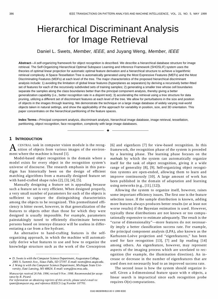
A top-level flow diagram for the processing done ineach of the Space-Tessellation Tree’s processing elementsduring the learning phase is given in Fig. 2. In order tominimize the limitation of our work to “well-framed” im-ages, we want to allow for some variations in the position,scale, and orientation of the objects in the training sam-ples. This can be accomplished either through more imageacquisition, but that is expensive in terms of time, storage,and cost. The images this system receives provides an at-tention point and scale to be used to extract a fovea imageof the object of interest. Rather than extracting just a singlefovea image from this attention point and scale, a familyof fovea images are generated by varying the attentionpoint and scale from the supplied points. This will allowthe system to learn some measure of positional and scalevariation in the training set.

Fig. 1. (a) A sample partitioning of the feature space; (b) The tree structure associated with the tessellation shown. Each cell in the partition doesnot need to cover a meaningful class. Each cell operates in a different feature space, and the leaf nodes give a final tessellation. This setup canapproximate virtually any complex decision region, and provides a logarithmic retrieval complexity.

Fig. 2. A top-level flow of the processing performed at each node in the Space-Tessellation Tree during the training phase. A set of training sam-ples which enter the processing element are extended to allow for learning-based generalization for position, scale, and orientation. These ex-tended samples are vectorized and used to produce the projection matrices to the MEF and MDF subspaces. The extended samples are pro-jected to the MDF subspace using these matrices, and a tessellation of the space covered by the node being worked on is produced. The projec-tion matrices and the space tessellation for each node are produced in the learning phase.


2.2 BackgroundThe SHOSLIF utilizes two derived feature sets: the MostExpressive Features (MEFs) and the Most DiscriminatingFeatures (MDFs) [31].

2.2.1 The Most Expressive Features (MEF)Each input subimage can be treated as a high dimensionalfeature vector by concatenating the rows of the subimagetogether, using each pixel as a single feature.

We can perform Principal Component Analysis on theset of training images [7], [32], [17]. This Principal Compo-nent Analysis utilizes the eigenvectors of the sample scattermatrix associated with the largest eigenvalues. These vec-tors are in the direction of the major variations in the sam-ples, and as such can be used as a basis set with which todescribe the image samples. Because they capture the majorvariations in the training data, they can express the sampleswell and can approximate the samples, where the recon-struction is very close to the original.

This LPA projection, also called the Karhunen-Loèveprojection, has been used to represent (e.g., Kirby and Si-rovich [33]) and recognize face images (e.g., Pentland et al.[7], [13]), for planning the illumination of objects for futurerecognition tasks (e.g., Murase and Nayar [29]), and in a lipreading system (e.g., Bregler and Omohundro [14]), amongothers. Since the features produced in this projection givethe minimum mean-square error for approximating an im-age [22], [34], [35] and show good performance in imagereconstruction [33], we call them the Most Expressive Fea-tures in contrast to the Most Discriminating Features de-scribed below.

2.2.2 The Most Discriminating Features (MDF)Although the MEF projection is well-suited to object repre-sentation, the features produced are not necessarily goodfor discriminating among classes defined by the set of sam-ples. The MEFs describe some major variations in the set ofsample images, such as those due to lighting direction;these variations may well be irrelevant to how the classesare divided.

If a labeling scheme is available for the training images,linear discriminant analysis (LDA) [17] can be performed,as in [36]. In LDA, the between-class scatter is maximizedwhile minimizing the within-class scatter. In other words,the samples for each class are projected to a space whereeach class is clustered more tightly together, and the sepa-ration between the class means is increased. The featuresobtained using a LDA projection optimally discriminateamong the classes represented in the training set, in thesense of linear transform [37], [21]. They are the eigenvec-tors of W – 1B associated with the largest eigenvalues, whereW and B are the within-class scatter and the between-classscatter matrices, respectively. Due to their optimality in dis-crimination among all possible linear features, we call themthe Most Discriminating Features (MDF). For a performancedifference comparison between the MEF and the MDFspaces, the reader is referred to [38].

The LDA procedure breaks down, however, when thenumber of samples is smaller than the dimensionality of thesample vectors. This problem can be resolved using the

Discriminant Karhunen-Loève projection [38], where theLDA is performed in the MEF space (i.e., the Karhunen-Loève space), where the degeneracy does not occur.

2.3 Space TessellationWe want to exploit the strengths of the MDF feature setwhile trying to overcome its limitations. At the same time,we want to provide an effective and efficient method forretrieval of images from the database. To effect this, theSHOSLIF produces a hierarchical space tessellation usingthe hyperplanes derived by the MDFs. The feature space ofall possible images is partitioned into cells of differing sizesas shown in Fig. 1. A cell at level l is subdivided intosmaller cells at level l + 1. The network structure that caneffect this recursive tessellation is a Space-Tessellation Treewhose nodes represent cells at the corresponding levels asshown in Fig. 1. The tree is built automatically during thelearning phase; this tree is used in the recognition phase tofind the model in the learned database that best approxi-mates an unknown image in approximately O(log n) time.

2.3.1 The Hierarchy Decomposes the ProblemThe tree structure is able to decompose the problem of LDAinto smaller, tractable problems. At the root node of thetree, where the entire database of samples are found, theclasses may not be separable using the LDA technique. Butbecause we do not attempt to completely separate theclasses at a single level, we can successfully solve the prob-lem in stages by breaking it down into simpler pieces.

The DKL projection does its best in separating classes,even for the case of many classes. When the database con-tains many classes, however, they may not be linearly sepa-rable. The Space-Tessellation Tree provides a mechanism fordealing with this problem. Children of a particular nodedecompose the difficult problem of separating many classesinto several smaller problems. At each node of the tree, theset of features found in the LDA procedure are specificallytuned to the set of samples found in the node. So althoughthe MDF space provides an optimal set of features for classselection in the sense of linear transform, this optimal setmay be insufficient to separate classes. But even if a nodecannot completely separate the classes, it can make a firstattempt at separation, dividing the samples among its chil-dren nodes. Then at this child level, since fewer samplesexist, the LDA procedure is more likely to succeed. Sincethis is applied recursively, eventually a successful separa-tion of classes is achieved as shown in Fig. 5.

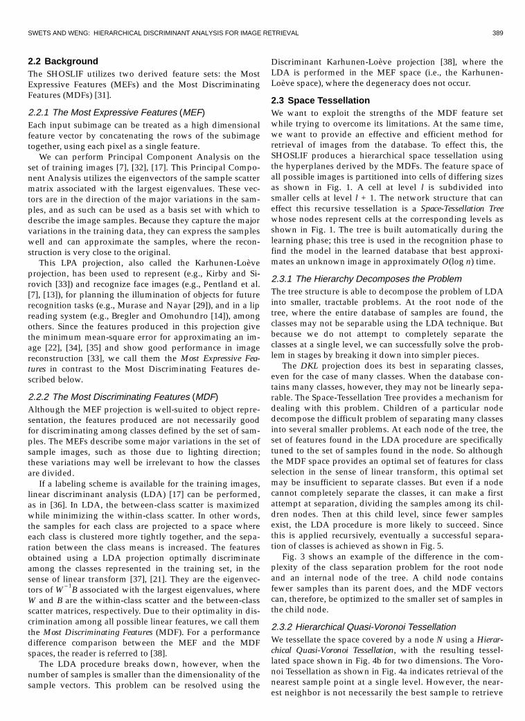
Fig. 3 shows an example of the difference in the com-plexity of the class separation problem for the root nodeand an internal node of the tree. A child node containsfewer samples than its parent does, and the MDF vectorscan, therefore, be optimized to the smaller set of samples inthe child node.

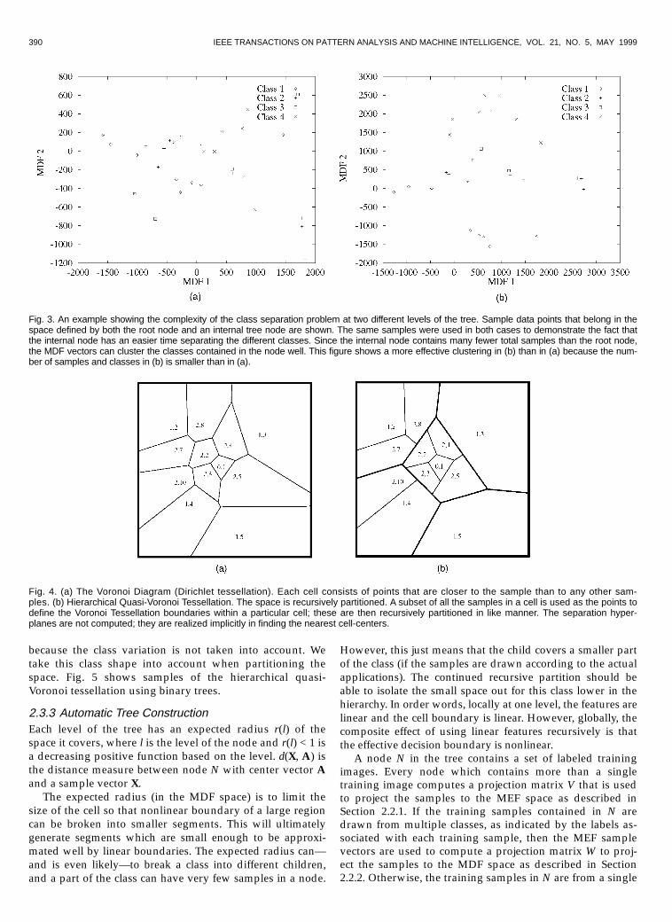
2.3.2 Hierarchical Quasi-Voronoi TessellationWe tessellate the space covered by a node N using a Hierar-chical Quasi-Voronoi Tessellation, with the resulting tessel-lated space shown in Fig. 4b for two dimensions. The Voro-noi Tessellation as shown in Fig. 4a indicates retrieval of thenearest sample point at a single level. However, the near-est neighbor is not necessarily the best sample to retrieve


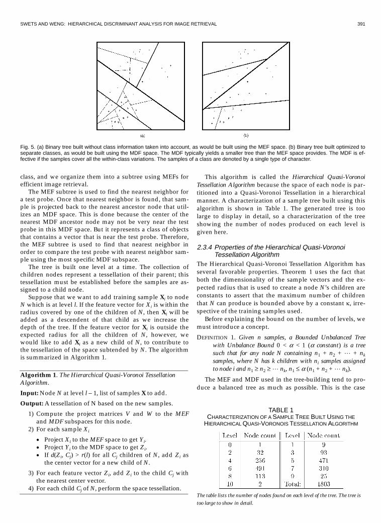
because the class variation is not taken into account. Wetake this class shape into account when partitioning thespace. Fig. 5 shows samples of the hierarchical quasi-Voronoi tessellation using binary trees.

2.3.3 Automatic Tree ConstructionEach level of the tree has an expected radius r(l) of thespace it covers, where l is the level of the node and r(l) < 1 isa decreasing positive function based on the level. d(X, A) isthe distance measure between node N with center vector Aand a sample vector X.

The expected radius (in the MDF space) is to limit thesize of the cell so that nonlinear boundary of a large regioncan be broken into smaller segments. This will ultimatelygenerate segments which are small enough to be approxi-mated well by linear boundaries. The expected radius can—and is even likely—to break a class into different children,and a part of the class can have very few samples in a node.

However, this just means that the child covers a smaller partof the class (if the samples are drawn according to the actualapplications). The continued recursive partition should beable to isolate the small space out for this class lower in thehierarchy. In order words, locally at one level, the features arelinear and the cell boundary is linear. However, globally, thecomposite effect of using linear features recursively is thatthe effective decision boundary is nonlinear.

A node N in the tree contains a set of labeled trainingimages. Every node which contains more than a singletraining image computes a projection matrix V that is usedto project the samples to the MEF space as described inSection 2.2.1. If the training samples contained in N aredrawn from multiple classes, as indicated by the labels as-sociated with each training sample, then the MEF samplevectors are used to compute a projection matrix W to proj-ect the samples to the MDF space as described in Section2.2.2. Otherwise, the training samples in N are from a single

Fig. 3. An example showing the complexity of the class separation problem at two different levels of the tree. Sample data points that belong in thespace defined by both the root node and an internal tree node are shown. The same samples were used in both cases to demonstrate the fact thatthe internal node has an easier time separating the different classes. Since the internal node contains many fewer total samples than the root node,the MDF vectors can cluster the classes contained in the node well. This figure shows a more effective clustering in (b) than in (a) because the num-ber of samples and classes in (b) is smaller than in (a).

Fig. 4. (a) The Voronoi Diagram (Dirichlet tessellation). Each cell consists of points that are closer to the sample than to any other sam-ples. (b) Hierarchical Quasi-Voronoi Tessellation. The space is recursively partitioned. A subset of all the samples in a cell is used as the points todefine the Voronoi Tessellation boundaries within a particular cell; these are then recursively partitioned in like manner. The separation hyper-planes are not computed; they are realized implicitly in finding the nearest cell-centers.


class, and we organize them into a subtree using MEFs forefficient image retrieval.

The MEF subtree is used to find the nearest neighbor fora test probe. Once that nearest neighbor is found, that sam-ple is projected back to the nearest ancestor node that util-izes an MDF space. This is done because the center of thenearest MDF ancestor node may not be very near the testprobe in this MDF space. But it represents a class of objectsthat contains a vector that is near the test probe. Therefore,the MEF subtree is used to find that nearest neighbor inorder to compare the test probe with nearest neighbor sam-ple using the most specific MDF subspace.

The tree is built one level at a time. The collection ofchildren nodes represent a tessellation of their parent; thistessellation must be established before the samples are as-signed to a child node.

Suppose that we want to add training sample Xi to nodeN which is at level l. If the feature vector for Xi is within theradius covered by one of the children of N, then Xi will beadded as a descendent of that child as we increase thedepth of the tree. If the feature vector for Xi is outside theexpected radius for all the children of N, however, wewould like to add Xi as a new child of N, to contribute tothe tessellation of the space subtended by N. The algorithmis summarized in Algorithm 1.

Algorithm 1. The Hierarchical Quasi-Voronoi TessellationAlgorithm.

Input: Node N at level l – 1, list of samples X to add.

Output: A tessellation of N based on the new samples.

1)�Compute the project matrices V and W to the MEFand MDF subspaces for this node.

2)�For each sample Xi

�� Project Xi to the MEF space to get Yi.�� Project Yi to the MDF space to get Zi.�� If d(Zi, Cj) > r(l) for all Cj children of N, add Zi as

the center vector for a new child of N.

3)�For each feature vector Zi, add Zi to the child Cj withthe nearest center vector.

4)�For each child Cj of N, perform the space tessellation.

This algorithm is called the Hierarchical Quasi-VoronoiTessellation Algorithm because the space of each node is par-titioned into a Quasi-Voronoi Tessellation in a hierarchicalmanner. A characterization of a sample tree built using thisalgorithm is shown in Table 1. The generated tree is toolarge to display in detail, so a characterization of the treeshowing the number of nodes produced on each level isgiven here.

2.3.4 Properties of the Hierarchical Quasi-VoronoiTessellation Algorithm

The Hierarchical Quasi-Voronoi Tessellation Algorithm hasseveral favorable properties. Theorem 1 uses the fact thatboth the dimensionality of the sample vectors and the ex-pected radius that is used to create a node N’s children areconstants to assert that the maximum number of childrenthat N can produce is bounded above by a constant k, irre-spective of the training samples used.

Before explaining the bound on the number of levels, wemust introduce a concept.

DEFINITION 1. Given n samples, a Bounded Unbalanced Treewith Unbalance Bound 0 < a < 1 (a constant) is a treesuch that for any node N containing n1 + n2 + L + nk

samples, where N has k children with ni samples assignedto node i and n1 � n2 � L nk, n1 � a (n1 + n2 + L nk).

The MEF and MDF used in the tree-building tend to pro-duce a balanced tree as much as possible. This is the case

Fig. 5. (a) Binary tree built without class information taken into account, as would be built using the MEF space. (b) Binary tree built optimized toseparate classes, as would be built using the MDF space. The MDF typically yields a smaller tree than the MEF space provides. The MDF is ef-fective if the samples cover all the within-class variations. The samples of a class are denoted by a single type of character.

TABLE 1CHARACTERIZATION OF A SAMPLE TREE BUILT USING THE

HIERARCHICAL QUASI-VORONOIS TESSELLATION ALGORITHM

The table lists the number of nodes found on each level of the tree. The tree istoo large to show in detail.


because the MEF and MDF attempts to partition the samplesin terms of the statistics of the distribution. The above defini-tion limits the degree of unbalancedness. If Algorithm 1 pro-duces a Bounded-Unbalanced tree, then Lemma 1 provesthat there are O(log n) levels. Note that there is no proof thatthe trees produced by Algorithm 1 must indeed be Bounded-Unbalanced; however, in our studies we have obtained em-perical evidence to suggest that they are.

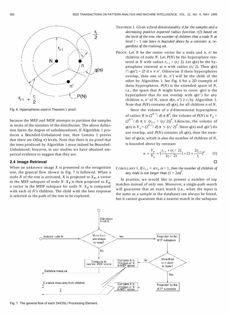
2.4 Image RetrievalWhen an unknown image X is presented to the recognitiontree, the general flow shown in Fig. 7 is followed. When anode N of the tree is activated, X is projected to XY, a vectorin the MEF subspace of node N. XY is then projected to XZ,a vector in the MDF subspace for node N. XZ is comparedwith each of N’s children. The child with the best responseis selected as the path of the tree to be explored.

THEOREM 1. Given a fixed dimensionality d for the samples and adecreasing positive expected radius function r(l) based onthe level of the tree, the number of children that a node N atlevel l - 1 can have is bounded above by a constant k, re-gardless of the training set.

PROOF. Let N be the center vector for a node and n, n’ bechildren of node N. Let P(N) be the hypersphere cen-tered at N with radius rl-1 + (rl/2). Let q(n) be the hy-persphere centered at n with radius (rl/2). Then q(n)> q(n’) = « if n � n’. Otherwise if these hyperspheresoverlap, then one of {n, n’} will be the child of theother by Algorithm 1. See Fig. 6 for a 2D example ofthese hyperspheres. P(N) is the extended space of N,i.e., the space that N might have to cover. q(n) is thehypersphere that do not overlap with q(n’�) for anychildren n, n’ of N, since d(n, n’) � rl by Algorithm 1.Note that P(N) contains all q(n), for all children n of N.

Since the volume of a d-dimensional hypersphereof radius R is (2d-1/d) p Rd, the volume of P(N) is Vp =(2d-1/d) p � (rl-1 + (rl/2))d. Likewise, the volume ofq(n) is Vq = (2d-1/d) p � (rl/2)d. Since q(n) and q(n’) donot overlap, and P(N) contains all q(n), then the num-ber of q(n)s, which is also the number of children of N,is bounded above by constant

k = =+

= +- -VV

r rr

rr

p

q

l l

l

l

l

d[( / )

( / ) ] [ ]1 122 1

2 . (1)

o

COROLLARY 1. If rl-1 = a rl, a > 1, then the number of children ofany node is not larger than (1 + 2a)d.

In practice, we would like to present a number of topmatches instead of only one. Moreover, a single-path searchwill guarantee that an exact match (i.e., when the input isthe same as a sample in the database) can always be found,but it cannot guarantee that a nearest match in the subspace

Fig. 7. The general flow of each SHOSLI Processing Element.

Fig. 6. Hyperspheres used in Theorem 1 proof.


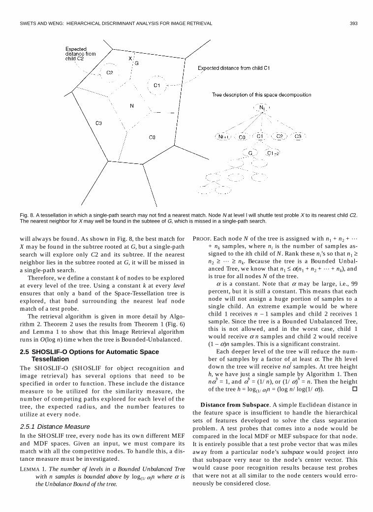
will always be found. As shown in Fig. 8, the best match forX may be found in the subtree rooted at G, but a single-pathsearch will explore only C2 and its subtree. If the nearestneighbor lies in the subtree rooted at G, it will be missed ina single-path search.

Therefore, we define a constant k of nodes to be exploredat every level of the tree. Using a constant k at every levelensures that only a band of the Space-Tessellation tree isexplored, that band surrounding the nearest leaf nodematch of a test probe.

The retrieval algorithm is given in more detail by Algo-rithm 2. Theorem 2 uses the results from Theorem 1 (Fig. 6)and Lemma 1 to show that this Image Retrieval algorithmruns in O(log n) time when the tree is Bounded-Unbalanced.

2.5 SHOSLIF-O Options for Automatic SpaceTessellation

The SHOSLIF-O (SHOSLIF for object recognition andimage retrieval) has several options that need to bespecified in order to function. These include the distancemeasure to be utilized for the similarity measure, thenumber of competing paths explored for each level of thetree, the expected radius, and the number features toutilize at every node.

2.5.1 Distance MeasureIn the SHOSLIF tree, every node has its own different MEFand MDF spaces. Given an input, we must compare itsmatch with all the competitive nodes. To handle this, a dis-tance measure must be investigated.

LEMMA 1. The number of levels in a Bounded Unbalanced Treewith n samples is bounded above by log(1/a)n where a isthe Unbalance Bound of the tree.

PROOF. Each node N of the tree is assigned with n1 + n2 + L+ nk samples, where ni is the number of samples as-signed to the ith child of N. Rank these ni’s so that n1 �n2 � L � nk. Because the tree is a Bounded Unbal-anced Tree, we know that n1 � a(n1 + n2 + L + nk), andis true for all nodes N of the tree.

a is a constant. Note that a may be large, i.e., 99percent, but it is still a constant. This means that eachnode will not assign a huge portion of samples to asingle child. An extreme example would be wherechild 1 receives n - 1 samples and child 2 receives 1sample. Since the tree is a Bounded Unbalanced Tree,this is not allowed, and in the worst case, child 1would receive a n samples and child 2 would receive(1 - a)n samples. This is a significant constraint.

Each deeper level of the tree will reduce the num-ber of samples by a factor of at least a. The lth leveldown the tree will receive nal samples. At tree heighth, we have just a single sample by Algorithm 1. Thennah = 1, and ah = (1/n), or (1/a)h = n. Then the heightof the tree h = log(1/a)n = (log n/log(1/a)). o

Distance from Subspace. A simple Euclidean distance inthe feature space is insufficient to handle the hierarchicalsets of features developed to solve the class separationproblem. A test probes that comes into a node would becompared in the local MDF or MEF subspace for that node.It is entirely possible that a test probe vector that was milesaway from a particular node’s subspace would project intothat subspace very near to the node’s center vector. Thiswould cause poor recognition results because test probesthat were not at all similar to the node centers would erro-neously be considered close.

Fig. 8. A tessellation in which a single-path search may not find a nearest match. Node N at level l will shuttle test proble X to its nearest child C2.The nearest neighbor for X may well be found in the subteee of G, which is missed in a single-path search.


Instead, we need to take into account the distance fromthe subspace being compared. Each node constructs a differ-ent set of subspaces based on the samples contained in thatnode. The Distance from Subspace (DFS) distance measuretakes into account the distance from the projection space inaddition to the distance of the projection to the node centers.

The DFS distance measure is given by

d X A X VV X VWW V X VWW V At t t t t( , ) = - + -2 2

where X is the test probe, A is the center vector, V is theprojection matrix to the MEF space, and W is the projection

matrix to the MDF space. So the product Y = VtX is theprojection of the test probe X onto the MEF subspace; VY =

VVtX represents this MEF projection in the original image

space. Likewise, Z = WtVtX is the projection of X onto the

MDF subspace, and VWZ = VWWtVtX represents this MDFprojection back in the original image space. Note that

computationally, for Z = WtVtX, AZ = WtVtA, and VW = M,

iMZ - MAZi2 = iM(Z - AZ)i2 = (Z - AZ)tMtM(Z - AZ). Thus,only a small matrix multiplication need be performed to

effect this distance measure. This MtM matrix can be pre-computed during the learning phase and stored in eachnode so that in the testing phase, the computational com-plexity of this operation is minimized.

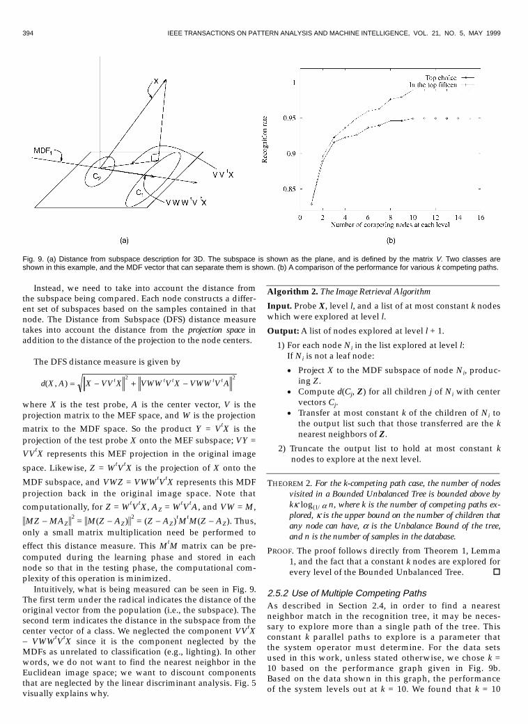
Intuitively, what is being measured can be seen in Fig. 9.The first term under the radical indicates the distance of theoriginal vector from the population (i.e., the subspace). Thesecond term indicates the distance in the subspace from thecenter vector of a class. We neglected the component VVtX- VWWtVtX since it is the component neglected by theMDFs as unrelated to classification (e.g., lighting). In otherwords, we do not want to find the nearest neighbor in theEuclidean image space; we want to discount componentsthat are neglected by the linear discriminant analysis. Fig. 5visually explains why.

Algorithm 2. The Image Retrieval Algorithm

Input. Probe X, level l, and a list of at most constant k nodeswhich were explored at level l.

Output: A list of nodes explored at level l + 1.

1)�For each node Ni in the list explored at level l:If Ni is not a leaf node:

�� Project X to the MDF subspace of node Ni, produc-ing Z.

�� Compute d(Cj, Z) for all children j of Ni with centervectors Cj.

�� Transfer at most constant k of the children of Ni tothe output list such that those transferred are the knearest neighbors of Z.

2) Truncate the output list to hold at most constant knodes to explore at the next level.

THEOREM 2. For the k-competing path case, the number of nodesvisited in a Bounded Unbalanced Tree is bounded above bykk log(1/a n, where k is the number of competing paths ex-plored, k is the upper bound on the number of children thatany node can have, a is the Unbalance Bound of the tree,and n is the number of samples in the database.

PROOF. The proof follows directly from Theorem 1, Lemma1, and the fact that a constant k nodes are explored forevery level of the Bounded Unbalanced Tree. o

2.5.2 Use of Multiple Competing PathsAs described in Section 2.4, in order to find a nearestneighbor match in the recognition tree, it may be neces-sary to explore more than a single path of the tree. Thisconstant k parallel paths to explore is a parameter thatthe system operator must determine. For the data setsused in this work, unless stated otherwise, we chose k =10 based on the performance graph given in Fig. 9b.Based on the data shown in this graph, the performanceof the system levels out at k = 10. We found that k = 10

Fig. 9. (a) Distance from subspace description for 3D. The subspace is shown as the plane, and is defined by the matrix V. Two classes areshown in this example, and the MDF vector that can separate them is shown. (b) A comparison of the performance for various k competing paths.


gives good runners-up for best matches at a low com-putational cost.

2.5.3 Expected RadiusNode N uses the expected radius r(l) to determine when itneeds to create a new child to accommodate a trainingsample. r(l) indicates the size of the cells that we would liketo achieve at level l. This expected radius is a decreasingpositive function based on the level of the tree. For thiswork, we have chosen r(l) = 1.336-l for node N on level l ofthe Space-Tessellation Tree. This number was chosen be-cause at the root node of the tree, i.e., at level l = 0, the ex-pected radius is 12,646.219. This radius is large enough tocover all of the samples in the data sets utilized in this work.

The value 1.3 was used as a base because it gave favorableresults in the shape of the tree. A tree that is too wide and fatproduces inefficiencies because many children must be ex-plored at a high level of the tree; a tree that is too thin and tallproduces inefficiences because many projections must bedone in order to find the nearest neighbor in the database.

3 EXPERIMENTAL RESULTS

In order to verify the proper functionality of the system, weexperimented with a large multifarious set of real-worldobjects found in natural scenes. In this section, we demon-strate the ability of the MDF space to tolerate within-classvariations and to discount such imaging artifacts as lightingdirection, and show how the tree structure provides theability for view-based recognition.

The images utilized for these experiments used a stan-dard fovea size of 88 × 64 pixels. So when vectorized, thedimensionality of the original input vectors were d = 5,632.When projected to the MEF space, utilizing 95 percent ofthe variance, at the root node, typically between 30 and 60principal components were utilized. Then when projectedto the MDF space, the number of discriminating vectorsutilized were limited to 5 or 95 percent of the variance forthe samples contained in the node, whichever was less.

3.1 Space ComparisonSince the analysis showed that the MDF space should per-form better than the MEF space (or the image space di-rectly), a study was performed to demonstrate this fact.Furthermore, though the hierarchy described provides effi-ciency to both the learning and retrieval phases, the recog-nition performance may suffer somewhat from not exam-ining all possibilities in the database. Therefore, a studywas also performed to examine the performance difference

between using a “flat” database, in which all images in thedatabase are examined for possible matches, and the de-scribed hierarchical database. Finally, the recognition per-formance will be dependent on whether a single MDF pro-jection is used, performing the space tessellation in this sin-gle space; or if a new MDF projection is performed at eachnode of the tree. A study examining the performance be-tween these two modes was also done.

The training images come from a set of real-world ob-jects in natural settings. At least two training images fromeach of 38 object classes were provided for a total of 108training images; a disjoint set of test images were used in allof the tests. For each of the tests performed, the identical setof training images and test images were used.

For those tests where subspaces are used, the DistanceFrom Subspace (DFS) distance metric was used, and 15nodes were explored at each level when using the treestructure.

3.1.1 Effects of the Feature Spaces and the TreeHierarchy

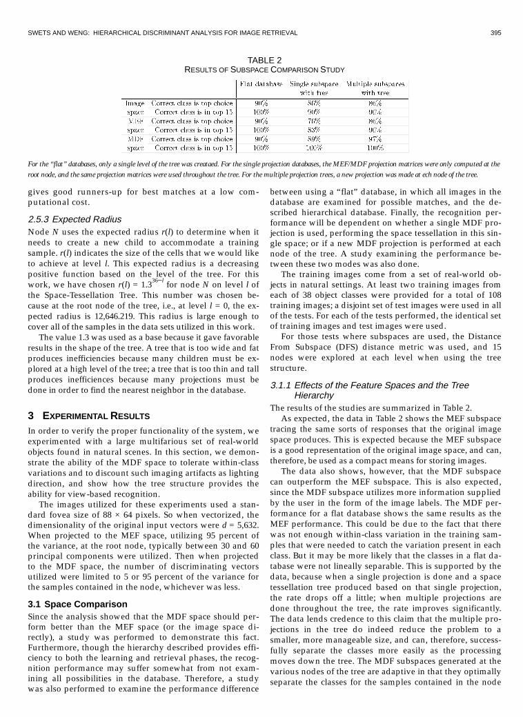
The results of the studies are summarized in Table 2.As expected, the data in Table 2 shows the MEF subspace

tracing the same sorts of responses that the original imagespace produces. This is expected because the MEF subspaceis a good representation of the original image space, and can,therefore, be used as a compact means for storing images.

The data also shows, however, that the MDF subspacecan outperform the MEF subspace. This is also expected,since the MDF subspace utilizes more information suppliedby the user in the form of the image labels. The MDF per-formance for a flat database shows the same results as theMEF performance. This could be due to the fact that therewas not enough within-class variation in the training sam-ples that were needed to catch the variation present in eachclass. But it may be more likely that the classes in a flat da-tabase were not lineally separable. This is supported by thedata, because when a single projection is done and a spacetessellation tree produced based on that single projection,the rate drops off a little; when multiple projections aredone throughout the tree, the rate improves significantly.The data lends credence to this claim that the multiple pro-jections in the tree do indeed reduce the problem to asmaller, more manageable size, and can, therefore, success-fully separate the classes more easily as the processingmoves down the tree. The MDF subspaces generated at thevarious nodes of the tree are adaptive in that they optimallyseparate the classes for the samples contained in the node

TABLE 2RESULTS OF SUBSPACE COMPARISON STUDY

For the “flat” databases, only a single level of the tree was creataed. For the single projection databases, the MEF/MDF projection matrices were only computed at theroot node, and the same projection matrices were used throughout the tree. For the multiple projection trees, a new projection was made at ech node of the tree.


in the sense of linear transform. As the processing movesalong the nodes of the tree, a different set of features tunedspecifically for those samples contained in the node areutilized for subclass selection.

3.2 Face DatabaseIn order to compare with the results of others in the com-munity utilizing eigenfeature methods, a test was per-formed on a database comprised of only faces.

The face database was organized by individual; eachindividual had a pool of images from which to drawtraining and test data sets. Each individual had at leasttwo images for training with a change of expression. Theimages of 38 individuals (182 images) came from the

Michigan State University Pattern Recognition and ImageProcessing laboratory. Images of individuals in this setwere taken under uncontrolled conditions, over severaldays, and under different lighting conditions. Classes of303 (654 images) came from the FERET database. All ofthese classes had at least two images of an individualtaken under controlled lighting, with a change of expres-sion. Twenty-four of these classes had additional imagestaken of the subjects on a different day with very poorcontrast. Sixteen classes (144 images) came from the MITMedia lab under identical lighting conditions (ambientlaboratory light). Twenty-nine classes (174 images) camefrom the Weizmann Institute, and are images with threevery controlled lighting conditions for each of two differ-ent expressions.

In this experiment, when an image that was used fortraining was also used as a test probe, such as is done withPhotobook [39], [13], [40] (i.e., resubstitution method), theSHOSLIF always retrieved the correct image as its firstchoice 100 percent of the time. The second image retrievedon a database of 1,042 face images was a correct match for98 percent of the test probes using the resubstitutionmethod, which is comparable to the Photobook [40] re-sponse rate on a different data set. Table 3 shows a sum-mary of the results obtained both by resubstituting thetraining samples as test probes and by using a disjoint set ofimages for testing.

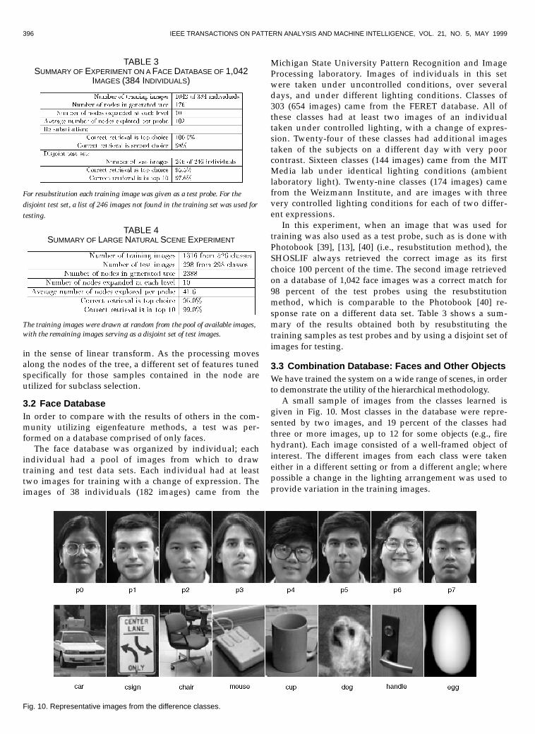
3.3 Combination Database: Faces and Other ObjectsWe have trained the system on a wide range of scenes, in orderto demonstrate the utility of the hierarchical methodology.

A small sample of images from the classes learned isgiven in Fig. 10. Most classes in the database were repre-sented by two images, and 19 percent of the classes hadthree or more images, up to 12 for some objects (e.g., firehydrant). Each image consisted of a well-framed object ofinterest. The different images from each class were takeneither in a different setting or from a different angle; wherepossible a change in the lighting arrangement was used toprovide variation in the training images.

TABLE 3SUMMARY OF EXPERIMENT ON A FACE DATABASE OF 1,042

IMAGES (384 INDIVIDUALS)

For resubstitution each training image was given as a test probe. For thedisjoint test set, a list of 246 images not found in the training set was used fortesting.

TABLE 4SUMMARY OF LARGE NATURAL SCENE EXPERIMENT

The training images were drawn at random from the pool of available images,with the remaining images serving as a disjoint set of test images.

Fig. 10. Representative images from the difference classes.


Following training, the system was tested using a test setcompletely disjoint from the training set of images. A sum-mary of the results are shown in Table 4.

The instances where the retrieval failed were due in largepart to significant differences in object shape and three-dimensional (3D) rotation.

3.4 Handling 2D VariationIn order to alleviate some of our reliance on well-framedimages, we want to train the system on a set of imageswhich contains some variations in the position, scale, andorientation of the objects of interest. This can be accom-plished by greatly increased image acquisition for pointssurrounding the fixation point and scale provided. The in-crease in image acquisition is expensive in terms of timeand storage space, however, and could instead be accom-plished by extending the training set for a grid of pointssurrounding the extracted fovea image in terms of the po-sition, scale, and 2D orientation foviation parameters. Eachfovea image comes from some attention mechanism thatspecifies a fixation point and a scale. This fixation point canbe overlaid with a grid in both the position and the scaleparameters, and a new fovea image extracted from theoriginal image at each of these grid points. Thus more varia-tion due to size and position can be handled by extracting aset of fovea images to add to the Space-Tessellation tree foreach grid point surrounding the attention point and scaleinstead of just extracting a single image.

Fig. 11 demonstrates the variability that the system canhandle by extending the training set in this manner. Whenthe training set is thus extended, the Space-Tessellationtree grows in size, but not by the factor of the increasednumber of samples. If we assume that the search tree pro-vides O(log s) levels for s training samples, then the treehas k log s levels for some constant k. Now if the number oftraining samples is expanded by 3 to handle the positionalvariation, and by 6 to handle the scale variation, then wehave a total of 36s samples to put into a tree. Then therewill be k log {36s} = k log 3 log 6 log s = k’ log s levels inthe Space-Tessellation Tree, for constant k’, which is stillO(log s) levels in the tree. Typical values for 3 will be 3 = 9

or 25 for a 3 × 3 or a 5 � 5 grid surrounding the attentionpoint, respectively; 6 will typically be 6 = 3 or 5 to deal withthe various scales. We have tested this approach to handlingpositional and scale variation on two different data sets.

3.4.1 Handling ScaleThe first data set is the full combination data set that de-scribed in Section 3.3 with more than 1,300 original trainingimages. We ran the experiment using P = 1 (i.e., on the atten-tion mechanism’s attention point alone) and�6 = 3 (i.e., 3 gridpoints surrounding the attention mechanism’s scale). Fortraining, we set the scale span to be 30 percent of the foveasize. That is, each grid point represented a 15 percent changein the fovea size, one training image at a 15 percent smallerscale than the attention mechanism dictated, one at the at-tention mechanism’s specified scale, and one at 15 percentlarger than the attention mechnism’s specified scale. Fortesting purposes, we took the disjoint test set described in 3.3and genrated a set of test images from this set with a randomscale change in ther ange of [–0, +20] percent of the foveasize. The characterization and results of this test is shown inTable 5. The table shows the difference between theperofrmance when the scaling was built into the trainingphase and when it was not. As can be seen from the data, for

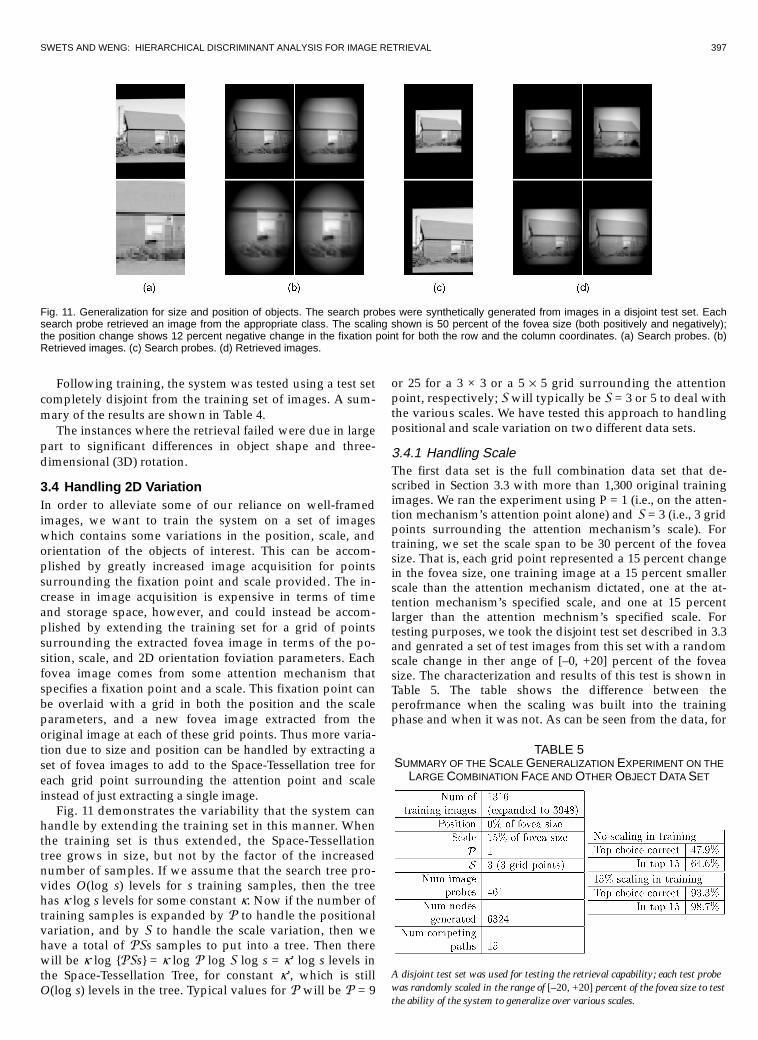
Fig. 11. Generalization for size and position of objects. The search probes were synthetically generated from images in a disjoint test set. Eachsearch probe retrieved an image from the appropriate class. The scaling shown is 50 percent of the fovea size (both positively and negatively);the position change shows 12 percent negative change in the fixation point for both the row and the column coordinates. (a) Search probes. (b)Retrieved images. (c) Search probes. (d) Retrieved images.

TABLE 5SUMMARY OF THE SCALE GENERALIZATION EXPERIMENT ON THE

LARGE COMBINATION FACE AND OTHER OBJECT DATA SET

A disjoint test set was used for testing the retrieval capability; each test probewas randomly scaled in the range of [–20, +20] percent of the fovea size to testthe ability of the system to generalize over various scales.


the test probes, either the attention supplier must correspondto the scaling done in the training phase, or the training setmust be expanded to include those images in the range ofscales that need to be properly retrieved. Fig. 12 shows anexample test probe and the images retrieved when scalingwas enabled for the training phase.

3.4.2 Handling Scale and PositionUtilizing the system on the large combination data set showsthe ability of the system both to operate on large image data-base sizes and to handle a specified variation in the scale ofthe extracted area of interest for an attention point and scale.To show the positional extension of the training data, asmaller original training set was used. For the second ex-periment in the demonstration of the system to handle 2Dparameter changes, the data set described in Section 3.1 wasused. Table 6 shows the data pursuant to this experiment.

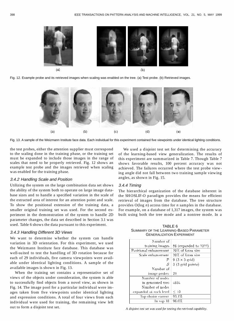
3.4.3 Handling Different 3D ViewsWe want to determine whether the system can handlevariation in 3D orientation. For this experiment, we usedthe Weizmann Institute face database. This database waswell-suited to test the handling of 3D rotation because foreach of 29 individuals, five camera viewpoints were avail-able under identical lighting conditions. A sample of theavailable images is shown in Fig. 13.

When the training set contains a representative set ofviews of the objects under consideration, the system is ableto successfully find objects from a novel view, as shown inFig. 14. The image pool for a particular individual were im-ages taken from five viewpoints under identical lightingand expression conditions. A total of four views from eachindividual were used for training, the remaining view leftout to form a disjoint test set.

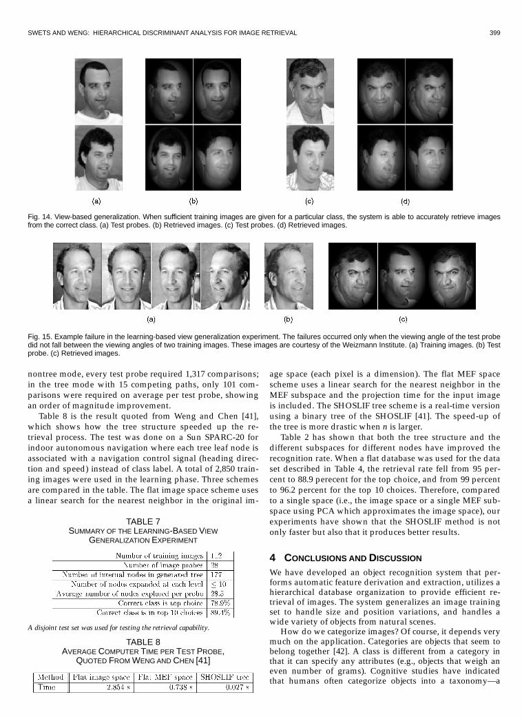
We used a disjoint test set for determining the accuracyof the learning-based view generalization. The results ofthis experiment are summarized in Table 7. Though Table 7shows favorable results, 100 percent accuracy was notachieved. The failures occurred where the test probe view-ing angle did not fall between two training sample viewingangles, as shown in Fig. 15.

3.4.4 TimingThe hierarchical organization of the database inherent inthe SHOSLIF-O paradigm provides the means for efficientretrieval of images from the database. The tree structureprovides O(log n) access time for n samples in the database.For example, on a database of 1,317 images, the system wasbuilt using both the tree mode and a nontree mode. In a

Fig. 12. Example probe and its retrieved images when scaling was enabled on the tree. (a) Test probe. (b) Retrieved images.

Fig. 13. A sample of the Weizmann Institute face data. Each individual for this experiment contained five viewpoints under identical lighting conditions.

TABLE 6SUMMARY OF THE LEARNING-BASED PARAMETER

GENERALIZATION EXPERIMENT

A disjoint test set was used for testing the retriveal capability.


nontree mode, every test probe required 1,317 comparisons;in the tree mode with 15 competing paths, only 101 com-parisons were required on average per test probe, showingan order of magnitude improvement.

Table 8 is the result quoted from Weng and Chen [41],which shows how the tree structure speeded up the re-trieval process. The test was done on a Sun SPARC-20 forindoor autonomous navigation where each tree leaf node isassociated with a navigation control signal (heading direc-tion and speed) instead of class label. A total of 2,850 train-ing images were used in the learning phase. Three schemesare compared in the table. The flat image space scheme usesa linear search for the nearest neighbor in the original im-

age space (each pixel is a dimension). The flat MEF spacescheme uses a linear search for the nearest neighbor in theMEF subspace and the projection time for the input imageis included. The SHOSLIF tree scheme is a real-time versionusing a binary tree of the SHOSLIF [41]. The speed-up ofthe tree is more drastic when n is larger.

Table 2 has shown that both the tree structure and thedifferent subspaces for different nodes have improved therecognition rate. When a flat database was used for the dataset described in Table 4, the retrieval rate fell from 95 per-cent to 88.9 perecent for the top choice, and from 99 percentto 96.2 percent for the top 10 choices. Therefore, comparedto a single space (i.e., the image space or a single MEF sub-space using PCA which approximates the image space), ourexperiments have shown that the SHOSLIF method is notonly faster but also that it produces better results.

4 CONCLUSIONS AND DISCUSSION

We have developed an object recognition system that per-forms automatic feature derivation and extraction, utilizes ahierarchical database organization to provide efficient re-trieval of images. The system generalizes an image trainingset to handle size and position variations, and handles awide variety of objects from natural scenes.

How do we categorize images? Of course, it depends verymuch on the application. Categories are objects that seem tobelong together [42]. A class is different from a category inthat it can specify any attributes (e.g., objects that weigh aneven number of grams). Cognitive studies have indicatedthat humans often categorize objects into a taxonomy—a

Fig. 14. View-based generalization. When sufficient training images are given for a particular class, the system is able to accurately retrieve imagesfrom the correct class. (a) Test probes. (b) Retrieved images. (c) Test probes. (d) Retrieved images.

Fig. 15. Example failure in the learning-based view generalization experiment. The failures occurred only when the viewing angle of the test probedid not fall between the viewing angles of two training images. These images are courtesy of the Weizmann Institute. (a) Training images. (b) Testprobe. (c) Retrieved images.

TABLE 7SUMMARY OF THE LEARNING-BASED VIEW

GENERALIZATION EXPERIMENT

A disjoint test set was used for testing the retrieval capability.

TABLE 8AVERAGE COMPUTER TIME PER TEST PROBE,

QUOTED FROM WENG AND CHEN [41]


hierarchy in which successive levels refer to increasinglymore specific objects. There is an intermediate level which ismore likely to be used to encode experience that superordi-nate or subordinate levels. For example, people use apple torefer to an experience rather than fruit or McIntosh apple [43].The method presented here could be used to organize imagesbased on an intermediate level of category that the users pre-fer to utilize. Retrieval with other superordinate or subordi-nate categories as well as other classifications schemes maybe realized using pointers from symbolic attribute tables tothe corresponding leaves of the SHOSLIF tree [44].

The automatic hierarchical discriminant analysismethod used in this work recursively decomposes ahuge, high-dimensional nonlinear problem into smaller,simpler, tractable problems. The hierarchical Quasi-Voronoi Tessellation provides a means for dividing thespace into smaller pieces for further analysis. This allowsthe DKL projection to produce better local features formore efficient and tractable subclass separation. TheSpace-Tessellation Tree introduced in this work providesa time complexity of O(log n) for a search for the bestmatch in a model database of n objects. This low com-plexity opens the door towards learning a huge databaseof objects.

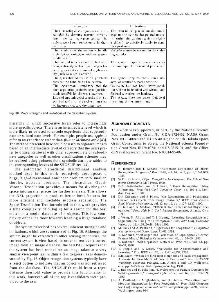
The system described has several inherent strengths andlimitations, which are summarized in Fig. 16. Although thesystem might be extended to other sensing modalities, thecurrent system is view-based: in order to retrieve a correctimage from an image database, the SHOSLIF requires thatthe system has been trained on an image taken at a verysimilar viewpoint (i.e., within a few degrees), as is demon-strated by Fig. 15. Object recognition systems typically havea reject option to indicate that an object was not retrievedfrom the database. The SHOSLIF-O could learn a rejectdistance threshold value to provide this functionality. Inthis work, however, all of the top k candidates were pro-vided to the user.

ACKNOWLEDGMENTS

This work was supported, in part, by the National ScienceFoundation under Grant No. CDA-9724462; NASA GrantNos. NGT-40046 and NGT5-40042; the South Dakota SpaceGrant Consortuim to Swets; the National Science Founda-tion Grant Nos. IRI 9410741 and IIS 9815191; and the Officeof Naval Research Grant No. N00014-95-06.

REFERENCES

[1]� K. Ikeuche and T. Kanade, “Automatic Generation of ObjectRecognition Programs,” Proc. IEEE, vol. 76, no. 8, pp. 1,016–1,035,1988.

[2]� W.E.L. Grimson, Object Recognition by Computer: The Role of Geo-metric Constraints. MIT Press, 1990.

[3]� D.P. Huttenlocher and S. Ullman, “Object Recognition UsingAlignment,” Proc. Int’l Conf. Computer Vision, pp. 102–111, Lon-don, England, 1987.

[4]� D.J. Kriegman and J. Ponce, “On Recognizing and PositioningCurved 3-D Objects from Image Contours,” IEEE Trans. PatternAnal. Machine Intelligence, vol. 12, no. 12, pp. 1,127–1,137, 1990.

[5]� F. Stein and G. Medioni, “Efficient Two Dimensional Object Rec-ognition,” Proc. 10th Int’l Conf. Pattern Recognition, Atlantic City,1990.

[6]� J. Weng, N. Ahuja, and T. S. Huang, “Learning Recognition andSegmentation Using the Cresceptron,” Proc. Int’l Conf. ComputerVision, pp. 121–128, Berlin, May 1993.

[7]� M. Turk and A. Pentland, “Eigenfaces for Rcognition,” J. CognitiveNeuroscience, vol. 3, no. 1, pp. 71–86, 1991.

[8]� T. Kohonen, “Self-Organized Formation of Topologically CorrectFeature Maps,” Biological Cybernetics, vol. 43, pp. 59–69, 1982.

[9]� T. Kohonen, “Self-Organized Network,” Proc. IEEE, vol. 43, pp.59–69, 1990.

[10]� T. Poggio and F. Girosi, “Networks for Approximation andLearning,” Proc. IEEE, vol. 78, pp. 1,481–1,497, 1990.

[11]� E.B. Baum, “When are k-Nearest Neighbor and Back PropagationAccurate for Feasible Sized Sets of Examples?” Proc. EURASIPWorkshop, Sezimbra, Portugal, L.B. Almedia and C.J. Wellekens,eds., pp. 2–25. New York: Springer-Verlag, 1990.

[12]� J. Rubner and K. Schulten, “Development of Feature Detectors bySelf-Organization,” Biological Cybernetics., vol. 62, pp. 193–199,1990.

[13]� A. Pentland, B. Moghaddam, and T. Starner, “View-Based andModular Eigenspaces for Face Recognition,” Proc. IEEE ComputerSoc. Conf. Computer Vision and Pattern Recognition, pp. 84–91, Seattle,Washington, June 994.

Fig. 16. Major strengths and limitations of the described system.


[14]� C. Bregler and S. M. Omohundro, “Nonlinear Manifold Learningfor Visual Speech Recognition,” Proc. Int’l Conf. Computer Vision,pp. 494–499, 1995.

[15]� L. Breiman, J.H. Friedman, R.A. Olshen, and C.J. Stone, Classifica-tion and Regression Trees. Chapman & Hall, 1993.

[16]� R. Duda and P. Hart, Pattern Classification and Scene Analysis. NewYork: John Wiley & Sons, 1973.

[17]� A.K. Jain and R.C. Dubes, Algorithms for Clustering Data.Englewood Cliffs, N.J.: Prentice Hall, 1988.

[18]� J. Quinlan, “Induction of Decision Trees,” Machine Learning, vol. 1,no. 1, pp. 81–106, 1986.

[19]� B.D. Ripley, Pattern Recognition and Neural Networks. New York:Cambridge Univ. Press, 1996.

[20]� D.J. Hand, Discrimination and Classification. Chichester: John Wiley& Sons, 1981.

[21]� S.S. Wilks, Math.l Statistics. New York: John Wiley & Sons, 1963.[22]� K. Fukunaga, Introduction to Statistical Pattern Recognition, second

edition, New York: Academic Press, 1990.[23]� G.R. Dattatreya and L.N. Kanal, “Decision Tress in Pattern Recog-

nition,” Progress in Pattern Recognition, L. Kanal and A. Rosenfeld,eds., pp. 189–239, New York: Elsevier Science, 1985.

[24]� S.R. Safavin and D. Landgrebe, “A Survey of Decision Tree Classi-fier Methodology,” IEEE Trans. Systems, Man and Cybernetics, vol.21, pp. 660–674, May/June 1991.

[25]� S.K. Murthy, “Automatic Construction of Decision Trees fromData: A Multidisciplinary Survey,” Data Mining and KnowledgeDiscovery, 1998.

[26]� L. Breiman, J. Friedman, R. Olshen, and C. Stone, Classification andRegression Trees. New York: Chapman & Hall, 1993.

[27]� E.G. Henrichon, jr. and K.S. Fu, “A Nonparametric MultivariatePartitioning Procedure for Pattern Classification,” IEEE Trans.Computers, vol. 18, pp. 614–624, July 1969.

[28]� J.H. Friedman, “A Recursive Partition Decision Rule for Non-parametric Classification,” IEEE Trans. Computers, vol. 26, pp.404–408, Apr. 1977.

[29]� H. Murase and S.K. Nayar, “Illumination Planning for ObjectRecognition in Structured Environments,” Proc. IEEE ComputerSoc. Conf. Computer Vision and Pattern Recognition, pp. 31–38, Seat-tle, Washington, June 1994.

[30]� D.L. Swets, B. Punch, and J.J. Weng, “Genetic Algorithms for Ob-ject Recognition in a Complex Scene,” Proc., Int’l Conf. Image Proc-essing, pp. 595–598, Washington, D.C., Oct. 1995.

[31]� D.L. Swets and J.J. Weng, “Using Discriminant Eigenfeatures forImage Retrieval,”{IEEE Trans. Pattern Analysis Machine Intelligence,vol. 18, pp. 831–836, Aug. 1996.

[32]� D.L. Swets and J.J. Weng, “Efficient Content-Based Image Re-trieval Using Automatic Feature Selection,” Proc., Int’l Symp.Computer Vision, pp. 85–90, Coral Gables, Fla., Nov. 1995.

[33]� M. Kirby and L. Sirovich, “Application of the Karhunen-Loèveprocedure for the characterization of human faces,” IEEE Trans.Pattern Analysis Machine Intelligence, vol. 12, pp. 103–108, Jan.1990.

[34]� I.T. Jolliffe, Principal Component Analysis. New York: Springer-Verlag, 1986.

[35]� M.M. Loève, Probability Theory. Princeton, N.J.: Van Nostrand,1955.

[36]� T. Hastie and R. Tibshirani, “Discriminant Adaptive NearestNeighbor Classification,” IEEE Trans. Pattern Analysis Machine In-telligence, vol. 18, pp. 607–616, June 1996.

[37]� R.A. Fisher, “The Statistical Utilization of Multiple Measure-ments,” Annals of Eugenics, vol. 8, pp. 376–386, 1938.

[38]� D.L. Swets and J.J. Weng, “SHOSLIF-O: SHOSLIF for Object Rec-ognition and Image Retrieval (phase II),” Technical Report CPS95-39, Dept. of Computer Science, Michigan State Univ., EastLansing, Mich., Oct. 1995.

[39]� A. Pentland, R.W. Picard, and S. Scarloff, “Photobook: Tools forContent-Based Manipulation of Image Databases,” SPIE Storageand Retrieval Image and Video Databases II, no. 2,185, San Jose,Feb. 1994.

[40]� B. Moghaddam and A. Pentland, “Maximum Liklihood Detectionof Faces and Hands,” Int’l Workshop Automatic Face- and Gesture-Recognition, M. Bichsel, ed., pp. 122–128, 1995.

[41]� J. Weng and S. Chen, “Incremental Learning for Vision-BasedNavigation,” Proc. Int’l Conf. Pattern Recognition, vol. IV, pp. 45–49,Vienna, Austria, Aug. 1996.

[42]� E.E. Smith, “Categorization,” Thinking, D.N. Osherson and E.E.Smith, eds., pp. 33–53, MIT Press, 1990.

[43]� E. Rosch, C. Mervis, D. Gray, D. Johnson, and P. Boyes-Braehm,“Basic Objects in Natural Categories,” Cognitive Psychology, vol. 3,pp. 382–439, 1976.

[44]� D. L. Swets, Y. Pathak, and J. J. Weng, “An Image Database Sys-tem for with Support for Traditional Alphanumeric Queries andContent-Based Queries by Example,” Multimedia Tools and Applica-tions, vol. 7, no. 3, 1998.

Daniel L. Swets (S’85–M’96) earned his BSdegree in computer science from Calvin Col-lege, Grand Rapids, Michigan in 1986, and theMS and PhD degrees in computer science fromMichigan State University in 1991 and 1996,respectively. From 1986-1987, he was a soft-ware engineer at Rockwell International,Downey, California, whre he worked on theSpace Shuttle Orbiter Backup Flight System.From 1987-1992, he was a software engineer atSmiths Industries, Grand Rapids, Michigan,

where he worked on software for aerospace applications. Concurrently,he was an instructor at both Grand Valley State University, Allendale,Michigan and the Grand Rapids Community College, Grand Rapids,Michigan. From 1992–1994, he was a teaching and research assistantat Michigan State University while pursuing his PhD degree, and anAmeritech fellow at Michigan State University from 1994-1995. In1995, he joined the teaching staff at Augustana College, Sioux Falls,South Dakota, where he is now an assistant professor of computerscience. He has been a NASA Space grant fellow from 1996–present.Concurrent with these activities, he has owned and operated a smallbusiness computer-consultant firm. His current research interests in-clude parallel processing, algorithms for remote sensing, computervision, and pattern recognition. He is a member of the IEEE and theIEEE Computer Society.

Juyang Weng (S’85–M’88) received his BSdegree from Fudan University, Shanghai, Peo-ple’s Republic of China, in 1982, and the MSand PhD degrees from the University of Illinoisat Urbana-Champaign, in 1985 and 1989, re-spectively, all in computer science. From 1984–1988, he was a research assistant at the Coor-dinated Science Laboratory, University of Illinoisat Urbana-Champaign. From 1989–1990, hewas a researcher at Centre de Recherche In-formatique de Montréal, Quebec, Canada, while

adjunctively with Ecole Polytechnique de Montréal. From 1990–1992,he held a visiting research assistant professor position at the Universityof Illinois at Urbana-Champaign. In 1992, he joined the Department ofComputer Science, Michigan State University, East Lansing, where heis now an associate professor. He is a coauthor of the book Motion andStructure from Image Sequences (Springer-Verlag, 1993). His currentresearch interests include computer vision, human-machine multimo-dal interface using vision, speech, gesture and actions, autonomouslearning robots, and automatic development of machine intelligence.He is a member of the IEEE and the IEEE Computer Society.

Documents

386 IEEE TRANSACTIONS ON PATTERN ANALYSIS …xrm.phys.northwestern.edu/research/pdf_papers/1999/swets...386 IEEE TRANSACTIONS ON PATTERN ANALYSIS AND MACHINE INTELLIGENCE, VOL. 21,