Embed Size (px)
Citation preview

8/8/2019 37997710 Hehner a Practical Theory of Programming 2004
http://slidepdf.com/reader/full/37997710-hehner-a-practical-theory-of-programming-2004 1/242
aPracticalTheory
of Programming
second edition
Eric C.R. Hehner

8/8/2019 37997710 Hehner a Practical Theory of Programming 2004
http://slidepdf.com/reader/full/37997710-hehner-a-practical-theory-of-programming-2004 2/242
–5
a
PracticalTheoryof
Programming
second edition2004 January 1
Eric C.R. Hehner
Department of Computer ScienceUniversity of TorontoToronto ON M5S 2E4
The first edition of this book was published bySpringer-Verlag Publishers
New York 1993
ISBN 0-387-94106-1QA76.6.H428
This second edition is available free at
www.cs.utoronto.ca/~hehner/aPToP
You may copy freely as long as youinclude all the information on this page.

8/8/2019 37997710 Hehner a Practical Theory of Programming 2004
http://slidepdf.com/reader/full/37997710-hehner-a-practical-theory-of-programming-2004 3/242
–4
Contents
0 Preface 0
0.0 Introduction 0
0.1 Second Edition 1
0.2 Quick Tour 1
0.3 Acknowledgements 2
1 Basic Theories 3
1.0 Boolean Theory 3
1.0.0 Axioms and Proof Rules 5
1.0.1 Expression and Proof Format 7
1.0.2 Monotonicity and Antimonotonicity 9
1.0.3 Context 10
1.0.4 Formalization 12
1.1 Number Theory 12
1.2 Character Theory 13
2 Basic Data Structures 14
2.0 Bunch Theory 14
2.1 Set Theory (optional) 17
2.2 String Theory 17
2.3 List Theory 20
2.3.0 Multidimensional Structures 22
3 Function Theory 23
3.0 Functions 23
3.0.0 Abbreviated Function Notations 25
3.0.1 Scope and Substitution 253.1 Quantifiers 26
3.2 Function Fine Points (optional) 28
3.2.0 Function Inclusion and Equality (optional) 30
3.2.1 Higher-Order Functions (optional) 30
3.2.2 Function Composition (optional) 31
3.3 List as Function 32
3.4 Limits and Reals (optional) 32
4 Program Theory 34
4.0 Specifications 34
4.0.0 Specification Notations 36
4.0.1 Specification Laws 37
4.0.2 Refinement 39
4.0.3 Conditions (optional) 40
4.0.4 Programs 41
4.1 Program Development 43
4.1.0 Refinement Laws 43
4.1.1 List Summation 43
4.1.2 Binary Exponentiation 45

8/8/2019 37997710 Hehner a Practical Theory of Programming 2004
http://slidepdf.com/reader/full/37997710-hehner-a-practical-theory-of-programming-2004 4/242
–3 Contents
4.2 Time 46
4.2.0 Real Time 46
4.2.1 Recursive Time 48
4.2.2 Termination 50
4.2.3 Soundness and Completeness (optional) 51
4.2.4 Linear Search 51
4.2.5 Binary Search 534.2.6 Fast Exponentiation 57
4.2.7 Fibonacci Numbers 59
4.3 Space 61
4.3.0 Maximum Space 63
4.3.1 Average Space 64
5 Programming Language 66
5.0 Scope 66
5.0.0 Variable Declaration 66
5.0.1 Variable Suspension 67
5.1 Data Structures 685.1.0 Array 68
5.1.1 Record 69
5.2 Control Structures 69
5.2.0 While Loop 69
5.2.1 Loop with Exit 71
5.2.2 Two-Dimensional Search 72
5.2.3 For Loop 74
5.2.4 Go To 76
5.3 Time and Space Dependence 76
5.4 Assertions (optional) 77
5.4.0 Checking 775.4.1 Backtracking 77
5.5 Subprograms 78
5.5.0 Result Expression 78
5.5.1 Function 79
5.5.2 Procedure 80
5.6 Alias (optional) 81
5.7 Probabilistic Programming (optional) 82
5.7.0 Random Number Generators 84
5.7.1 Information (optional) 87
5.8 Functional Programming (optional) 88
5.8.0 Function Refinement 89
6 Recursive Definition 91
6.0 Recursive Data Definition 91
6.0.0 Construction and Induction 91
6.0.1 Least Fixed-Points 94
6.0.2 Recursive Data Construction 95
6.1 Recursive Program Definition 97
6.1.0 Recursive Program Construction 98
6.1.1 Loop Definition 99

8/8/2019 37997710 Hehner a Practical Theory of Programming 2004
http://slidepdf.com/reader/full/37997710-hehner-a-practical-theory-of-programming-2004 5/242
Contents –2
7 Theory Design and Implementation 100
7.0 Data Theories 100
7.0.0 Data-Stack Theory 100
7.0.1 Data-Stack Implementation 101
7.0.2 Simple Data-Stack Theory 102
7.0.3 Data-Queue Theory 103
7.0.4 Data-Tree Theory 1047.0.5 Data-Tree Implementation 104
7.1 Program Theories 106
7.1.0 Program-Stack Theory 106
7.1.1 Program-Stack Implementation 106
7.1.2 Fancy Program-Stack Theory 107
7.1.3 Weak Program-Stack Theory 107
7.1.4 Program-Queue Theory 108
7.1.5 Program-Tree Theory 108
7.2 Data Transformation 110
7.2.0 Security Switch 112
7.2.1 Take a Number 1137.2.2 Limited Queue 115
7.2.3 Soundness and Completeness (optional) 117
8 Concurrency 118
8.0 Independent Composition 118
8.0.0 Laws of Independent Composition 120
8.0.1 List Concurrency 120
8.1 Sequential to Parallel Transformation 121
8.1.0 Buffer 122
8.1.1 Insertion Sort 123
8.1.2 Dining Philosophers 124
9 Interaction 126
9.0 Interactive Variables 126
9.0.0 Thermostat 128
9.0.1 Space 129
9.1 Communication 131
9.1.0 Implementability 132
9.1.1 Input and Output 133
9.1.2 Communication Timing 134
9.1.3 Recursive Communication (optional) 134
9.1.4 Merge 135
9.1.5 Monitor 136
9.1.6 Reaction Controller 137
9.1.7 Channel Declaration 138
9.1.8 Deadlock 139
9.1.9 Broadcast 140

8/8/2019 37997710 Hehner a Practical Theory of Programming 2004
http://slidepdf.com/reader/full/37997710-hehner-a-practical-theory-of-programming-2004 6/242
–1 Contents
10 Exercises 147
10.0 Basic Theories 147
10.1 Basic Data Structures 154
10.2 Function Theory 156
10.3 Program Theory 161
10.4 Programming Language 177
10.5 Recursive Definition 18110.6 Theory Design and Implementation 187
10.7 Concurrency 193
10.8 Interaction 195
11 Reference 201
11.0 Justifications 201
11.0.0 Notation 201
11.0.1 Boolean Theory 201
11.0.2 Bunch Theory 202
11.0.3 String Theory 203
11.0.4 Function Theory 20411.0.5 Program Theory 204
11.0.6 Programming Language 206
11.0.7 Recursive Definition 207
11.0.8 Theory Design and Implementation 207
11.0.9 Concurrency 208
11.0.10 Interaction 208
11.1 Sources 209
11.2 Bibliography 211
11.3 Index 215
11.4 Laws 223
11.4.0 Booleans 22311.4.1 Generic 225
11.4.2 Numbers 225
11.4.3 Bunches 226
11.4.4 Sets 227
11.4.5 Strings 227
11.4.6 Lists 228
11.4.7 Functions 228
11.4.8 Quantifiers 229
11.4.9 Limits 231
11.4.10 Specifications and Programs 231
11.4.11 Substitution 232
11.4.12 Conditions 232
11.4.13 Refinement 232
11.5 Names 233
11.6 Symbols 234
11.7 Precedence 235
End of Contents

8/8/2019 37997710 Hehner a Practical Theory of Programming 2004
http://slidepdf.com/reader/full/37997710-hehner-a-practical-theory-of-programming-2004 7/242
0
0 Preface
0.0 Introduction
What good is a theory of programming? Who wants one? Thousands of programmers program
every day without any theory. Why should they bother to learn one? The answer is the same as
for any other theory. For example, why should anyone learn a theory of motion? You can movearound perfectly well without one. You can throw a ball without one. Yet we think it important
enough to teach a theory of motion in high school.
One answer is that a mathematical theory gives a much greater degree of precision by providing a
method of calculation. It is unlikely that we could send a rocket to Jupiter without a mathematical
theory of motion. And even baseball pitchers are finding that their pitch can be improved by hiring
an expert who knows some theory. Similarly a lot of mundane programming can be done without
the aid of a theory, but the more difficult programming is very unlikely to be done correctly
without a good theory. The software industry has an overwhelming experience of buggy
programs to support that statement. And even mundane programming can be improved by the use
of a theory.
Another answer is that a theory provides a kind of understanding. Our ability to control and
predict motion changes from an art to a science when we learn a mathematical theory. Similarly
programming changes from an art to a science when we learn to understand programs in the same
way we understand mathematical theorems. With a scientific outlook, we change our view of the
world. We attribute less to spirits or chance, and increase our understanding of what is possible
and what is not. It is a valuable part of education for anyone.
Professional engineering maintains its high reputation in our society by insisting that, to be a
professional engineer, one must know and apply the relevant theories. A civil engineer must know
and apply the theories of geometry and material stress. An electrical engineer must know andapply electromagnetic theory. Software engineers, to be worthy of the name, must know and
apply a theory of programming.
The subject of this book sometimes goes by the name “programming methodology”, “science of
programming”, “logic of programming”, “theory of programming”, “formal methods of program
development”, or “verification”. It concerns those aspects of programming that are amenable to
mathematical proof. A good theory helps us to write precise specifications, and to design
programs whose executions provably satisfy the specifications. We will be considering the state of
a computation, the time of a computation, the memory space required by a computation, and the
interactions with a computation. There are other important aspects of software design and
production that are not touched by this book: the management of people, the user interface,documentation, and testing.
The first usable theory of programming, often called “Hoare's Logic”, is still probably the most
widely known. In it, a specification is a pair of predicates: a precondition and postcondition (these
and all technical terms will be defined in due course). A closely related theory is Dijkstra's
weakest precondition predicate transformer, which is a function from programs and postconditions
to preconditions, further advanced in Back's Refinement Calculus. Jones's Vienna Development
Method has been used to advantage in some industries; in it, a specification is a pair of predicates
(as in Hoare's Logic), but the second predicate is a relation. There are theories that specialize in
real-time programming, some in probabilistic programming, some in interactive programming.

8/8/2019 37997710 Hehner a Practical Theory of Programming 2004
http://slidepdf.com/reader/full/37997710-hehner-a-practical-theory-of-programming-2004 8/242
The theory in this book is simpler than any of those just mentioned. In it, a specification is just a
boolean expression. Refinement is just ordinary implication. This theory is also more general than
those just mentioned, applying to both terminating and nonterminating computation, to both
sequential and parallel computation, to both stand-alone and interactive computation. All at the
same time, we can have variables whose initial and final values are all that is of interest, variables
whose values are continuously of interest, variables whose values are known only
probabilistically, and variables that account for time and space. They all fit together in one theory
whose basis is the standard scientific practice of writing a specification as a boolean expression
whose (nonlocal) variables are whatever is considered to be of interest.
There is an approach to program proving that exhaustively tests all inputs, called model-checking.
Its advantage over the theory in this book is that it is fully automated. With a clever representation
of boolean expressions (see Exercise 6), model-checking currently boasts that it can explore up to
about 1060 states. That is more than the estimated number of atoms in the universe! It is an
impressive number until we realize that 1060 is about 2200 , which means we are talking about
200 bits. That is the state space of six 32-bit variables. To use model-checking on any program
with more than six variables requires abstraction; each abstraction requires proof that it preserves
the properties of interest, and these proofs are not automatic. To be practical, model-checkingmust be joined with other methods of proving, such as those in this book.
The emphasis throughout this book is on program development with proof at each step, rather than
on proof after development.
End of Introduction
0.1 Second Edition
In the second edition of this book, there is new material on space bounds, and on probabilistic
programming. The for-loop rule has been generalized. The treatment of concurrency has been
simplified. And for cooperation between parallel processes, there is now a choice: communication(as in the first edition), and interactive variables, which are the formally tractable version of shared
memory. Explanations have been improved throughout the book, and more worked examples
have been added.
As well as additions, there have been deletions. Any material that was usually skipped in a course
has been removed to keep the book short. It's really only 147 pages; after that is just exercises
and reference material.
Lecture slides and solutions to exercises are available to course instructors from the author.
End of Second Edition
0.2 Quick Tour
All technical terms used in this book are explained in this book. Each new term that you should
learn is underlined. As much as possible, the terminology is descriptive rather than honorary
(notable exception: “boolean”). There are no abbreviations, acronyms, or other obscurities of
language to annoy you. No specific previous mathematical knowledge or programming experience
is assumed. However, the preparatory material on booleans, numbers, lists, and functions in
Chapters 1, 2, and 3 is brief, and previous exposure might be helpful.
1 0 Preface

8/8/2019 37997710 Hehner a Practical Theory of Programming 2004
http://slidepdf.com/reader/full/37997710-hehner-a-practical-theory-of-programming-2004 9/242
The following chart shows the dependence of each chapter on previous chapters.
1 2 3 4 6 7
8 9
5
Chapter 4, Program Theory, is the heart of the book. After that, chapters may be selected oromitted according to interest and the chart. The only deviations from the chart are that Chapter 9
uses variable declaration presented in Subsection 5.0.0, and small optional Subsection 9.1.3
depends on Chapter 6. Within each chapter, sections and subsections marked as optional can be
omitted without much harm to the following material.
Chapter 10 consists entirely of exercises grouped according to the chapter in which the necessary
theory is presented. All the exercises in the section “Program Theory” can be done according to
the methods presented in Chapter 4; however, as new methods are presented in later chapters,
those same exercises can be redone taking advantage of the later material.
At the back of the book, Chapter 11 contains reference material. Section 11.0, “Justifications”,answers questions about earlier chapters, such as: why was this presented that way? why was
this presented at all? why wasn't something else presented instead? It may be of interest to
teachers and researchers who already know enough theory of programming to ask such questions.
It is probably not of interest to students who are meeting formal methods for the first time. If you
find yourself asking such questions, don't hesitate to consult the justifications.
Chapter 11 also contains an index of terminology and a complete list of all laws used in the book.
To a serious student of programming, these laws should become friends, on a first name basis.
The final pages list all the notations used in the book. You are not expected to know these
notations before reading the book; they are all explained as we come to them. You are welcome to
invent new notations if you explain their use. Sometimes the choice of notation makes all thedifference in our ability to solve a problem.
End of Quick Tour
0.3 Acknowledgements
For inspiration and guidance I thank Working Group 2.3 (Programming Methodology) of the
International Federation for Information Processing, particularly Edsger Dijkstra, David Gries,
Tony Hoare, Jim Horning, Cliff Jones, Bill McKeeman, Carroll Morgan, Greg Nelson, John
Reynolds, and Wlad Turski; I especially thank Doug McIlroy for encouragement. I thank my
graduate students and teaching assistants from whom I have learned so much, especially Ray
Blaak, Benet Devereux, Lorene Gupta, Peter Kanareitsev, Yannis Kassios, Victor Kwan, AlbertLai, Chris Lengauer, Andrew Malton, Theo Norvell, Rich Paige, Dimi Paun, Mark Pichora, Hugh
Redelmeier, and Alan Rosenthal. For their critical and helpful reading of the first draft I am most
grateful to Wim Hesselink, Jim Horning, and Jan van de Snepscheut. For good ideas I thank
Ralph Back, Eike Best, Wim Feijen, Netty van Gasteren, Nicolas Halbwachs, Gilles Kahn, Leslie
Lamport, Alain Martin, Joe Morris, Martin Rem, Pierre-Yves Schobbens, Mary Shaw, Bob
Tennent, and Jan Tijmen Udding. For reading the draft and suggesting improvements I thank
Jules Desharnais, Andy Gravell, Peter Lauer, Ali Mili, Bernhard Möller, Helmut Partsch, Jørgen
Steensgaard-Madsen, and Norbert Völker. I thank my class for finding errors.
End of Acknowledgements
End of Preface
0 Preface 2

8/8/2019 37997710 Hehner a Practical Theory of Programming 2004
http://slidepdf.com/reader/full/37997710-hehner-a-practical-theory-of-programming-2004 10/242
3
1 Basic Theories
1.0 Boolean Theory
Boolean Theory, also known as logic, was designed as an aid to reasoning, and we will use it to
reason about computation. The expressions of Boolean Theory are called boolean expressions.
We divide boolean expressions into two classes; those in one class are called theorems, and thosein the other are called antitheorems.
The expressions of Boolean Theory can be used to represent statements about the world; the
theorems represent true statements, and the antitheorems represent false statements. That is the
original application of the theory, the one it was designed for, and the one that supplies most of the
terminology. Another application for which Boolean Theory is perfectly suited is digital circuit
design. In that application, boolean expressions represent circuits; theorems represent circuits
with high voltage output, and antitheorems represent circuits with low voltage output.
The two simplest boolean expressions are and . The first one, , is a theorem, and the
second one, , is an antitheorem. When Boolean Theory is being used for its original purpose,we pronounce as “true” and as “false” because the former represents an arbitrary true
statement and the latter represents an arbitrary false statement. When Boolean Theory is being
used for digital circuit design, we pronounce and as “high voltage” and “low voltage”, or
as “power” and “ground”. They are sometimes called the “boolean values”; they may also be
called the “nullary boolean operators”, meaning that they have no operands.
There are four unary (one operand) boolean operators, of which only one is interesting. Its
symbol is ¬ , pronounced “not”. It is a prefix operator (placed before its operand). An
expression of the form ¬ x is called a negation. If we negate a theorem we obtain an antitheorem;
if we negate an antitheorem we obtain a theorem. This is depicted by the following truth table.
¬
Above the horizontal line, means that the operand is a theorem, and means that the operand
is an antitheorem. Below the horizontal line, means that the result is a theorem, and means
that the result is an antitheorem.
There are sixteen binary (two operand) boolean operators. Mainly due to tradition, we will use
only six of them, though they are not the only interesting ones. These operators are infix (placed
between their operands). Here are the symbols and some pronunciations.
∧“and”∨ “or”
⇒ “implies”, “is equal to or stronger than”
⇐ “follows from”, “is implied by”, “is weaker than or equal to”
= “equals”, “if and only if”
“differs from”, “is unequal to”, “exclusive or”, “boolean plus”
An expression of the form x∧ y is called a conjunction, and the operands x and y are called
conjuncts. An expression of the form x∨ y is called a disjunction, and the operands are called
disjuncts. An expression of the form x⇒ y is called an implication, x is called the antecedent,
and y is called the consequent. An expression of the form x⇐ y is also called an implication, but
now x is the consequent and y is the antecedent. An expression of the form x= y is called an

8/8/2019 37997710 Hehner a Practical Theory of Programming 2004
http://slidepdf.com/reader/full/37997710-hehner-a-practical-theory-of-programming-2004 11/242
equation, and the operands are called the left side and the right side. An expression of the form
x y is called an unequation, and again the operands are called the left side and the right side.
The following truth table shows how the classification of boolean expressions formed with binary
operators can be obtained from the classification of the operands. Above the horizontal line, the
pair means that both operands are theorems; the pair means that the left operand is a
theorem and the right operand is an antitheorem; and so on. Below the horizontal line, means
that the result is a theorem, and means that the result is an antitheorem.
∧ ∨
⇒
⇐
=
Infix operators make some expressions ambiguous. For example, ∧ ∨ might be read as
the conjunction ∧ , which is an antitheorem, disjoined with , resulting in a theorem. Or itmight be read as conjoined with the disjunction ∨ , resulting in an antitheorem. To say
which is meant, we can use parentheses: either ( ∧ ) ∨ or ∧ ( ∨ ) . To prevent a
clutter of parentheses, we employ a table of precedence levels, listed on the final page of the book.
In the table, ∧ can be found on level 9, and ∨ on level 10; that means, in the absence of
parentheses, apply ∧ before ∨ . The example ∧ ∨ is therefore a theorem.
Each of the operators = ⇒ ⇐ appears twice in the precedence table. The large versions = ⇒ ⇐ on level 16 are applied after all other operators. Except for precedence, the small versions and
large versions of these operators are identical. Used with restraint, these duplicate operators can
sometimes improve readability by reducing the parenthesis clutter still further. But a word of
caution: a few well-chosen parentheses, even if they are unnecessary according to precedence, canhelp us see structure. Judgement is required.
There are 256 ternary (three operand) operators, of which we show only one. It is called
conditional composition, and written if x then y else z . Here is its truth table.
if then else
For every natural number n , there are 22n operators of n operands, but we now have quite
enough.
When we stated earlier that a conjunction is an expression of the form x∧ y , we were using x∧ y
to stand for all expressions obtained by replacing the variables x and y with arbitrary boolean
expressions. For example, we might replace x with ( ⇒ ¬( ∨ )) and replace y with
( ∨ ) to obtain the conjunction
( ⇒ ¬( ∨ )) ∧ ( ∨ )
Replacing a variable with an expression is called subst itut ion or instantiation. With the
understanding that variables are there to be replaced, we admit variables into our expressions,
being careful of the following two points.
1 Basic Theories 4

8/8/2019 37997710 Hehner a Practical Theory of Programming 2004
http://slidepdf.com/reader/full/37997710-hehner-a-practical-theory-of-programming-2004 12/242
• We sometimes have to insert parentheses around expressions that are replacing variables in
order to maintain the precedence of operators. In the example of the preceding paragraph,
we replaced a conjunct x with an implication ⇒ ¬( ∨ ) ; since conjunction comes
before implication in the precedence table, we had to enclose the implication in parentheses.
We also replaced a conjunct y with a disjunction ∨ , so we had to enclose the
disjunction in parentheses.
• When the same variable occurs more than once in an expression, it must be replaced by the
same expression at each occurrence. From x ∧ x we can obtain ∧ , but not ∧ .
However, different variables may be replaced by the same or different expressions. From
x∧ y we can obtain both ∧ and ∧ .
As we present other theories, we will introduce new boolean expressions that make use of the
expressions of those theories, and classify the new boolean expressions. For example, when we
present Number Theory we will introduce the number expressions 1+1 and 2 , and the boolean
expression 1+1=2 , and we will classify it as a theorem. We never intend to classify a boolean
expression as both a theorem and an antitheorem. A statement about the world cannot be both true
and (in the same sense) false; a circuit's output cannot be both high and low voltage. If, byaccident, we do classify a boolean expression both ways, we have made a serious error. But it is
perfectly legitimate to leave a boolean expression unclassified. For example, 1/0=5 will be
neither a theorem nor an antitheorem. An unclassified boolean expression may correspond to a
statement whose truth or falsity we do not know or do not care about, or to a circuit whose output
we cannot predict. A theory is called consistent if no boolean expression is both a theorem and an
antitheorem, and inconsistent if some boolean expression is both a theorem and an antitheorem. A
theory is called complete if every fully instantiated boolean expression is either a theorem or an
antitheorem, and incomplete if some fully instantiated boolean expression is neither a theorem nor
an antitheorem.
1.0.0 Axioms and Proof Rules
We present a theory by saying what its expressions are, and what its theorems and antitheorems
are. The theorems and antitheorems are determined by the five rules of proof. We state the rules
first, then discuss them after.
Axiom Rule If a boolean expression is an axiom, then it is a theorem. If a boolean
expression is an antiaxiom, then it is an antitheorem.
Evaluation Rule If all the boolean subexpressions of a boolean expression are classified, then it
is classified according to the truth tables.
Completion Rule If a boolean expression contains unclassified boolean subexpressions, and all
ways of classifying them place it in the same class, then it is in that class.
Consistency Rule If a classified boolean expression contains boolean subexpressions, and only
one way of classifying them is consistent, then they are classified that way.
Instance Rule If a boolean expression is classified, then all its instances have that same
classification.
5 1 Basic Theories

8/8/2019 37997710 Hehner a Practical Theory of Programming 2004
http://slidepdf.com/reader/full/37997710-hehner-a-practical-theory-of-programming-2004 13/242
An axiom is a boolean expression that is stated to be a theorem. An antiaxiom is similarly a
boolean expression stated to be an antitheorem. The only axiom of Boolean Theory is and the
only antiaxiom is . So, by the Axiom Rule, is a theorem and is an antitheorem. As we
present more theories, we will give their axioms and antiaxioms; they, together with the other
rules of proof, will determine the new theorems and antitheorems of the new theory.
Before the invention of formal logic, the word “axiom” was used for a statement whose truth was
supposed to be obvious. In modern mathematics, an axiom is part of the design and presentation
of a theory. Different axioms may yield different theories, and different theories may have
different applications. When we design a theory, we can choose any axioms we like, but a bad
choice can result in a useless theory.
The entry in the top left corner of the truth table for the binary operators does not say ∧ = .
It says that the conjunction of any two theorems is a theorem. To prove that ∧ = is a
theorem requires the boolean axiom (to prove that is a theorem), the first entry on the ∧ row
of the truth table (to prove that ∧ is a theorem), and the first entry on the = row of the truth
table (to prove that ∧ = is a theorem).
The boolean expression
∨ xcontains an unclassified boolean subexpression, so we cannot use the Evaluation Rule to tell us
which class it is in. If x were a theorem, the Evaluation Rule would say that the whole
expression is a theorem. If x were an antitheorem, the Evaluation Rule would again say that the
whole expression is a theorem. We can therefore conclude by the Completion Rule that the whole
expression is indeed a theorem. The Completion Rule also says that
x ∨ ¬ xis a theorem, and when we come to Number Theory, that
1/0 = 5 ∨ ¬ 1/0 = 5
is a theorem. We do not need to know that a subexpression is unclassified to use the CompletionRule. If we are ignorant of the classification of a subexpression, and we suppose it to be
unclassified, any conclusion we come to by the use of the Completion Rule will still be correct.
In a classified boolean expression, if it would be inconsistent to place a boolean subexpression in
one class, then the Consistency Rule says it is in the other class. For example, suppose we know
that expression0 is a theorem, and that expression0 ⇒ expression1 is also a theorem. Can we
determine what class expression1 is in? If expression1 were an antitheorem, then by the
Evaluation Rule expression0 ⇒ expression1 would be an antitheorem, and that would be
inconsistent. So, by the Consistency Rule, expression1 is a theorem. This use of the
Consistency Rule is traditionally called “detachment” or “modus ponens”. As another example, if
¬expression is a theorem, then the Consistency Rule says that expression is an antitheorem.
Thanks to the negation operator and the Consistency Rule, we never need to talk about antiaxioms
and antitheorems. Instead of saying that expression is an antitheorem, we can say that
¬expression is a theorem. But a word of caution: if a theory is incomplete, it is possible that
neither expression nor ¬expression is a theorem. Thus “antitheorem” is not the same as “not a
theorem”. Our preference for theorems over antitheorems encourages some shortcuts of speech.
We sometimes state a boolean expression, such as 1+1=2 , without saying anything about it;
when we do so, we mean that it is a theorem. We sometimes say we will prove something,
meaning we will prove it is a theorem.
End of Axioms and Proof Rules
1 Basic Theories 6
8/8/2019 37997710 Hehner a Practical Theory of Programming 2004
http://slidepdf.com/reader/full/37997710-hehner-a-practical-theory-of-programming-2004 14/242
With our two axioms ( and ¬ ) and five proof rules we can now prove theorems. Some
theorems are useful enough to be given a name and be memorized, or at least be kept in a handy
list. Such a theorem is called a law. Some laws of Boolean Theory are listed at the back of the
book. Laws concerning ⇐ have not been included, but any law that uses ⇒ can be easily
rearranged into one using ⇐ . All of them can be proven using the Completion Rule, classifying
the variables in all possible ways, and evaluating each way. When the number of variables is more
than about 2, this kind of proof is quite inefficient. It is much better to prove new laws by making
use of already proven old laws. In the next subsection we see how.
1.0.1 Expression and Proof Format
The precedence table on the final page of this book tells how to parse an expression in the absence
of parentheses. To help the eye group the symbols properly, it is a good idea to leave space for
absent parentheses. Consider the following two ways of spacing the same expression.
a∧b ∨ ca ∧ b∨c
According to our rules of precedence, the parentheses belong around a∧b , so the first spacing is
helpful and the second misleading.
An expression that is too long to fit on one line must be broken into parts. There are several
reasonable ways to do it; here is one suggestion. A long expression in parentheses can be broken
at its main connective, which is placed under the opening parenthesis. For example,
( first part ∧ second part )
A long expression without parentheses can be broken at its main connective, which is placed under
where the opening parenthesis belongs. For example,
first part = second part
Attention to format makes a big difference in our ability to understand a complex expression.
A proof is a boolean expression that is clearly a theorem. One form of proof is a continuing
equation with hints.
expression0 hint 0
= expression1 hint 1
= expression2 hint 2
= expression3If we did not use equations in this continuing fashion, we would have to write
expression0 = expression1∧ expression1 = expression2
∧ expression2 = expression3The hints on the right side of the page are used, when necessary, to help make it clear that this
continuing equation is a theorem. The best kind of hint is the name of a law. The “hint 0” is
supposed to make it clear that expression0 = expression1 is a theorem. The “hint 1” is supposed
to make it clear that expression1 = expression2 is a theorem. And so on. By the transitivity of
=, this proof proves the theorem expression0 = expression3 .
7 1 Basic Theories

8/8/2019 37997710 Hehner a Practical Theory of Programming 2004
http://slidepdf.com/reader/full/37997710-hehner-a-practical-theory-of-programming-2004 15/242
Here is an example. Suppose we want to prove the first Law of Portation
a ∧ b ⇒ c = a ⇒ (b ⇒ c)
using only previous laws in the list at the back of this book. Here is a proof.
a ∧ b ⇒ c Material Implication
= ¬(a ∧ b) ∨ c Duality
= ¬a ∨ ¬b ∨ c Material Implication
=a ⇒ ¬b ∨ c Material Implication
= a ⇒ (b ⇒ c)
From the first line of the proof, we are told to use “Material Implication”, which is the first of the
Laws of Inclusion. This law says that an implication can be changed to a disjunction if we also
negate the antecedent. Doing so, we obtain the second line of the proof. The hint now is
“Duality”, and we see that the third line is obtained by replacing ¬(a ∧ b) with ¬a ∨ ¬b in
accordance with the first of the Duality Laws. By not using parentheses on the third line, we
silently use the Associative Law of disjunction, in preparation for the next step. The next hint is
again “Material Implication”; this time it is used in the opposite direction, to replace the first
disjunction with an implication. And once more, “Material Implication” is used to replace the
remaining disjunction with an implication. Therefore, by transitivity of = , we conclude that the
first Law of Portation is a theorem.
Here is the proof again, in a different form.
(a ∧ b ⇒ c = a ⇒ (b ⇒ c)) Material Implication, 3 times
= (¬(a ∧ b) ∨ c = ¬a ∨ (¬b ∨ c)) Duality
= (¬a ∨ ¬b ∨ c = ¬a ∨ ¬b ∨ c) Reflexivity of ==
The final line is a theorem, hence each of the other lines is a theorem, and in particular, the first line
is a theorem. This form of proof has some advantages over the earlier form. First, it makes proof
the same as simplification to . Second, although any proof in the first form can be written in the
second form, the reverse is not true. For example, the proof
(a⇒b = a∧b) = a Associative Law for == (a⇒b = (a∧b = a)) a Law of Inclusion
=cannot be converted to the other form. And finally, the second form, simplification to , can be
used for theorems that are not equations; the main operator of the boolean expression can be
anything, including ∧ , ∨ , or ¬ .
Sometimes it is clear enough how to get from one line to the next without a hint, and in that case no
hint will be given. Hints are optional, to be used whenever they are helpful. Sometimes a hint is
too long to fit on the remainder of a line. We may have
expression0 short hint
= expression1 and now a very long hint, written just as this is written,on as many lines as necessary, followed by
= expression2We cannot excuse an inadequate hint by the limited space on one line.
End of Expression and Proof Format
1 Basic Theories 8

8/8/2019 37997710 Hehner a Practical Theory of Programming 2004
http://slidepdf.com/reader/full/37997710-hehner-a-practical-theory-of-programming-2004 16/242
1.0.2 Monotonicity and Antimonotonicity
A proof can be a continuing equation, as we have seen; it can also be a continuing implication, or a
continuing mixture of equations and implications. As an example, here is a proof of the first Law
of Conflation, which says
(a ⇒ b) ∧ (c ⇒ d ) ⇒ a ∧ c ⇒ b ∧ d The proof goes this way: starting with the right side,
a ∧ c ⇒ b ∧ d distribute ⇒ over second ∧= (a ∧ c ⇒ b) ∧ (a ∧ c ⇒ d ) antidistribution twice
= ((a⇒b) ∨ (c⇒b)) ∧ ((a⇒d ) ∨ (c⇒d )) distribute ∧ over ∨ twice
= (a⇒b)∧(a⇒d ) ∨ (a⇒b)∧(c⇒d ) ∨ (c⇒b)∧(a⇒d ) ∨ (c⇒b)∧(c⇒d ) generalization
⇐ (a⇒b) ∧ (c⇒d )From the mutual transitivity of = and ⇐ , we have proven
a ∧ c ⇒ b ∧ d ⇐ (a⇒b) ∧ (c⇒d )which can easily be rearranged to give the desired theorem.
The implication operator is reflexive a⇒a , antisymmetric (a⇒b) ∧ (b⇒a) = (a=b) , and
transitive (a⇒b) ∧ (b⇒c) ⇒ (a⇒c) . It is therefore an ordering (just like ≤ for numbers). Wepronounce a⇒b either as “ a implies b ”, or, to emphasize the ordering, as “ a is stronger than
or equal to b ”. The words “stronger” and “weaker” may have come from a philosophical origin;
we ignore any meaning they may have other than the boolean order, in which is stronger than
. For clarity and to avoid philosophical discussion, it would be better to say “falser” rather than
“stronger”, and to say “truer” rather than “weaker”, but we use the standard terms.
The Monotonic Law a⇒b ⇒ c∧a ⇒ c∧b can be read (a little carelessly) as follows: if a is
weakened to b , then c∧a is weakened to c∧b . (To be more careful, we should say “weakened
or equal”.) If we weaken a , then we weaken c∧a . Or, the other way round, if we strengthen
b, then we strengthen c∧b . Whatever happens to a conjunct (weaken or strengthen), the same
happens to the conjunction. We say that conjunction is monotonic in its conjuncts.
The Antimonotonic Law a⇒b ⇒ (b⇒c) ⇒ (a⇒c) says that whatever happens to an antecedent
(weaken or strengthen), the opposite happens to the implication. We say that implication is
antimonotonic in its antecedent.
Here are the monotonic and antimonotonic properties of boolean expressions.
¬a is antimonotonic in aa∧b is monotonic in a and monotonic in b
a∨b is monotonic in a and monotonic in ba⇒b is antimonotonic in a and monotonic in b
a⇐b is monotonic in a and antimonotonic in bif a then b else c is monotonic in b and monotonic in c
These properties are useful in proofs. For example, in Exercise 2(k), to prove ¬(a ∧ ¬(a∨b)) ,
we can employ the Law of Generalization a ⇒ a∨b to strengthen a∨b to a . That weakens
¬(a∨b) and that weakens a ∧ ¬(a∨b) and that strengthens ¬(a ∧ ¬(a∨b)) .
¬(a ∧ ¬(a∨b)) use the Law of Generalization
⇐ ¬(a ∧ ¬a) now use the Law of Contradiction
=We thus prove that ¬(a ∧ ¬(a∨b)) ⇐ , and by an identity law, that is the same as proving
¬(a∧ ¬(a∨b)) . In other words, ¬(a ∧ ¬(a∨b)) is weaker than or equal to , and since there
9 1 Basic Theories

8/8/2019 37997710 Hehner a Practical Theory of Programming 2004
http://slidepdf.com/reader/full/37997710-hehner-a-practical-theory-of-programming-2004 17/242
is nothing weaker than , it is equal to . When we drive toward , the left edge of the proof
can be any mixture of = and ⇐ signs.
Similarly we can drive toward , and then the left edge of the proof can be any mixture of =
and ⇒ signs. For example,
a ∧ ¬(a∨b) use the Law of Generalization
⇒a ∧ ¬a now use the Law of Contradiction
=This is called “proof by contradiction”. It proves a ∧ ¬(a∨b) ⇒ , which is the same as
proving ¬(a ∧ ¬(a∨b)) . Any proof by contradiction can be converted to a proof by simplification
to at the cost of one ¬ sign per line.
End of Monotonicity and Antimonotonicity
1.0.3 Context
A proof, or part of a proof, can make use of local assumptions. A proof may have the format
assumption
⇒ ( expression0= expression1= expression2= expression3 )
for example. The step expression0 = expression1 can make use of the assumption just as
though it were an axiom. So can the step expression1 = expression2 , and so on. Within the
parentheses we have a proof; it can be any kind of proof including one that makes further local
assumptions. We thus can have proofs within proofs, indenting appropriately. If the subproof is
proving expression0 = expression3 , then the whole proof is proving
assumption ⇒ (expression0 = expression3)
If the subproof is proving expression0 , then the whole proof is proving
assumption ⇒ expression0If the subproof is proving , then the whole proof is proving
assumption ⇒which is equal to ¬assumption . Once again, this is “proof by contradiction”.
We can also use if then else as a proof, or part of a proof, in a similar manner. The format is
if possibility
then ( first subproof
assuming possibilityas a local axiom )
else ( second subproof
assuming ¬ possibilityas a local axiom )
If the first subproof proves something and the second proves anotherthing , the whole proof
proves
if possibility then something else anotherthingIf both subproofs prove the same thing, then by the Case Idempotent Law, so does the whole
proof, and that is its most frequent use.
1 Basic Theories 10
8/8/2019 37997710 Hehner a Practical Theory of Programming 2004
http://slidepdf.com/reader/full/37997710-hehner-a-practical-theory-of-programming-2004 18/242
Consider a step in a proof that looks like this:
expression0 ∧ expression1
= expression0 ∧ expression2When we are changing expression1 into expression2 , we can assume expression0 as a local
axiom just for this step. If expression0 really is a theorem, then we have done no harm by
assuming it as a local axiom. If, however, expression0 is an antitheorem, then both
expression0∧ expression1 and expression0 ∧ expression2 are antitheorems no matter what
expression1 and expression2 are, so again we have done nothing wrong. Symmetrically, when
proving
expression0 ∧ expression1= expression2 ∧ expression1
we can assume expression1 as a local axiom. However, when proving
expression0 ∧ expression1
= expression2 ∧ expression3we cannot assume expression0 to prove expression1=expression3 and in the same step assume
expression1 to prove expression0=expression2 . For example, starting from a ∧ a , we can
assume the first a and so change the second one to ,
a ∧ a assume first a to simplify second a= a ∧
or we can assume the second a and so change the first one to ,
a ∧ a assume second a to simplify first a= ∧ a
but we cannot assume both of them at the same time.
a ∧ a this step is wrong
= ∧
In this paragraph, the equal signs could have been implications in either direction.
Here is a list of context rules for proof.
In expression0 ∧ expression1 , when changing expression0 , we can assume expression1 .In expression0 ∧ expression1 , when changing expression1 , we can assume expression0 .
In expression0 ∨ expression1 , when changing expression0 , we can assume ¬expression1 .
In expression0 ∨ expression1 , when changing expression1 , we can assume ¬expression0 .
In expression0 ⇒ expression1 , when changing expression0 , we can assume ¬expression1 .
In expression0 ⇒ expression1 , when changing expression1 , we can assume expression0 .
In expression0 ⇐ expression1 , when changing expression0 , we can assume expression1 .
In expression0 ⇐ expression1 , when changing expression1 , we can assume ¬expression0 .
In if expression0 then expression1 else expression2 , when changing expression1 ,
we can assume expression0 .
In if expression0 then expression1 else expression2 , when changing expression2 ,
we can assume ¬expression0 .
In the previous subsection we proved Exercise 2(k): ¬(a ∧ ¬(a∨b)) . Here is another proof, this
time using context.
¬(a ∧ ¬(a∨b)) assume a to simplify ¬(a∨b)
= ¬(a ∧ ¬( ∨b)) Symmetry Law and Base Law for ∨= ¬(a ∧ ¬ ) Truth Table for ¬= ¬(a ∧ ) Base Law for ∧= ¬ Boolean Axiom, or Truth Table for ¬=
End of Context
11 1 Basic Theories

8/8/2019 37997710 Hehner a Practical Theory of Programming 2004
http://slidepdf.com/reader/full/37997710-hehner-a-practical-theory-of-programming-2004 19/242
1.0.4 Formalization
We use computers to solve problems, or to provide services, or just for fun. The desired computer
behavior is usually described at first informally, in a natural language (like English), perhaps with
some diagrams, perhaps with some hand gestures, rather than formally, using mathematical
formulas (notations). In the end, the desired computer behavior is described formally as a
program. A programmer must be able to translate informal descriptions to formal ones.
A statement in a natural language can be vague, ambiguous, or subtle, and can rely on a great deal
of cultural context. This makes formalization difficult, but also necessary. We cannot possibly
say how to formalize, in general; it requires a thorough knowledge of the natural language, and is
always subject to argument. In this subsection we just point out a few pitfalls in the translation
from English to boolean expressions.
The best translation may not be a one-for-one substitution of symbols for words. The same word
in different places may be translated to different symbols, and different words may be translated to
the same symbol. The words “and”, “also”, “but”, “yet”, “however”, and “moreover” might all be
translated as ∧ . Just putting things next to each other sometimes means ∧ . For example,“They're red, ripe, and juicy, but not sweet.” becomes red ∧ ripe ∧ juicy ∧ ¬sweet .
The word “or” in English is sometimes best translated as ∨ , and sometimes as . For example,
“They're either small or rotten.” probably includes the possibility that they're both small and
rotten, and should be translated as small ∨ rotten . But “Either we eat them or we preserve them.”
probably excludes doing both, and is best translated as eat preserve .
The word “if” in English is sometimes best translated as ⇒ , and sometimes as = . For example,
“If it rains, we'll stay home.” probably leaves open the possibility that we might stay home even if
it doesn't rain, and should be translated as rain ⇒ home . But “If it snows, we can go skiing.”
probably also means “and if it doesn't, we can't”, and is best translated as snow = ski . End of Formalization
End of Boolean Theory
1.1 Number Theory
Number Theory, also known as arithmetic, was designed to represent quantity. In the version we
present, a number expression is formed in the following ways.
a sequence of one or more decimal digits
∞ “infinity”
+ x “plus x ”
– x “minus x ” x + y “ x plus y ”
x – y “ x minus y ”
x × y “ x times y ”
x / y “ x divided by y ”
x y “ x to the power y ”
if a then x else ywhere x and y are any number expressions, and a is any boolean expression. The infinite
number expression ∞ will be essential when we talk about the execution time of programs. We
also introduce several new ways of forming boolean expressions:
1 Basic Theories 12

8/8/2019 37997710 Hehner a Practical Theory of Programming 2004
http://slidepdf.com/reader/full/37997710-hehner-a-practical-theory-of-programming-2004 20/242
x < y “ x is less than y ”
x ≤ y “ x is less than or equal to y ”
x > y “ x is greater than y ”
x ≥ y “ x is greater than or equal to y ”
x = y “ x equals y ”, “ x is equal to y ”
x y “ x differs from y ”, “ x is unequal to y ”
The axioms of Number Theory are listed at the back of the book. It's a long list, but most of them
should be familiar to you already. Notice particularly the two axioms
–∞ ≤ x ≤ ∞ extremes
–∞ < x ⇒ ∞+ x = ∞ absorption
Number Theory is incomplete. For example, the boolean expressions 1/0 = 5 and 0 < (–1)1/2
can neither be proven nor disproven.
End of Number Theory
1.2 Character Theory
The simplest character expressions are written as a prequote followed by a graphical shape. Forexample, `A is the “capital A” character, `1 is the “one” character, ` is the “space” character,
and `` is the “prequote” character. Character Theory is trivial. It has operators succ (successor),
pred (predecessor), and = < ≤ > ≥ if then else . We leave the details of this theory to the
reader's inclination.
End of Character Theory
All our theories use the operators = if then else , so their laws are listed at the back of the
book under the heading “Generic”, meaning that they are part of every theory. These laws are not
needed as axioms of Boolean Theory; for example, x= x can be proven using the Completion and
Evaluation rules. But in Number Theory and other theories, they are axioms; without them we
cannot even prove 5=5 .
The operators < ≤ > ≥ apply to some, but not all, types of expression. Whenever they do apply,
their axioms, as listed under the heading “Generic” at the back of the book, go with them.
End of Basic Theories
We have talked about boolean expressions, number expressions, and character expressions. In the
following chapters, we will talk about bunch expressions, set expressions, string expressions, list
expressions, function expressions, predicate expressions, relation expressions, specification
expressions, and program expressions; so many expressions. For brevity in the following
chapters, we will often omit the word “expression”, just saying boolean, number, character,
bunch, set, string, list, function, predicate, relation, specification, and program, meaning in eachcase a type of expression. If this bothers you, please mentally insert the word “expression”
wherever you would like it to be.
13 1 Basic Theories

8/8/2019 37997710 Hehner a Practical Theory of Programming 2004
http://slidepdf.com/reader/full/37997710-hehner-a-practical-theory-of-programming-2004 21/242
14
2 Basic Data Structures
A data structure is a collection, or aggregate, of data. The data may be booleans, numbers,
characters, or data structures. The basic kinds of structuring we consider are packaging and
indexing. These two kinds of structure give us four basic data structures.
unpackaged, unindexed: bunch
packaged, unindexed: setunpackaged, indexed: string
packaged, indexed: list
2.0 Bunch Theory
A bunch represents a collection of objects. For contrast, a set represents a collection of objects in a
package or container. A bunch is the contents of a set. These vague descriptions are made precise
as follows.
Any number, character, or boolean (and later also set, string of elements, and list of elements) is an
elementary bunch, or el ement. For example, the number 2 is an elementary bunch, orsynonymously, an element. Every expression is a bunch expression, though not all are
elementary.
From bunches A and B we can form the bunches
A , B “ A union B ”
A ‘ B “ A intersection B ”
and the number
¢ A “size of A ”, “cardinality of A ”
and the boolean
A: B “ A is in B ”, “ A is included in B ”
The size of a bunch is the number of elements it includes. Elements are bunches of size 1 .
¢2 = 1
¢(0, 2, 5, 9) = 4
Here are three quick examples of bunch inclusion.
2: 0, 2, 5, 9
2: 2
2, 9: 0, 2, 5, 9
The first says that 2 is in the bunch consisting of 0, 2, 5, 9 . The second says that 2 is in the
bunch consisting of only 2 . Note that we do not say “a bunch contains its elements”, but rather
“a bunch consists of its elements”. The third example says that both 2 and 9 are in 0, 2, 5, 9 ,
or in other words, the bunch 2, 9 is included in the bunch 0, 2, 5, 9 .
Here are the axioms of Bunch Theory. In these axioms, x and y are elements (elementary
bunches), and A , B , and C are arbitrary bunches.
x: y = x= y elementary axiom
x: A, B = x: A ∨ x: B compound axiom
A, A = A idempotence
A, B = B, A symmetry

8/8/2019 37997710 Hehner a Practical Theory of Programming 2004
http://slidepdf.com/reader/full/37997710-hehner-a-practical-theory-of-programming-2004 22/242
A,( B,C ) = ( A, B),C associativity
A‘ A = A idempotence
A‘ B = B‘ A symmetry
A‘( B‘C ) = ( A‘ B)‘C associativity
A, B: C = A: C ∧ B: C A: B‘C = A: B ∧ A: C
A: A, B generalization A‘ B: A specialization
A: A reflexivity
A: B ∧ B: A = A= B antisymmetry
A: B ∧ B: C ⇒ A: C transitivity
¢ x = 1 size
¢( A, B) + ¢( A‘ B) = ¢ A + ¢ B size
¬ x: A ⇒ ¢( A‘ x) = 0 size
A: B ⇒ ¢ A ≤ ¢ B size
From these axioms, many laws can be proven. Among them:
A,( A‘ B) = A absorption A‘( A, B) = A absorption
A: B ⇒ C , A: C , B monotonicity
A: B ⇒ C ‘ A: C ‘ B monotonicity
A: B = A, B = B = A = A‘ B inclusion
A,( B,C ) = ( A, B),( A,C ) distributivity
A,( B‘C ) = ( A, B)‘( A,C ) distributivity
A‘( B,C ) = ( A‘ B), ( A‘C ) distributivity
A‘( B‘C ) = ( A‘ B)‘( A‘C ) distributivity
A: B ∧ C : D ⇒ A,C : B, D conflation
A: B ∧ C : D ⇒ A‘C : B‘ D conflation
Here are several bunches that we will find useful:
null the empty bunch
bool = , the booleans
nat = 0, 1, 2, ... the natural numbers
int = ..., –2, –1, 0, 1, 2, ... the integer numbers
rat = ..., –1, 0, 2/3, ... the rational numbers
real = . . . the real numbers
xnat = 0, 1, 2, ..., ∞ the extended naturals
xint = –∞, ..., –2, –1, 0, 1, 2, ..., ∞ the extended integers
xrat = –∞, ..., –1, 0, 2/3, ..., ∞ the extended rationals
xreal = –∞, ..., ∞ the extended realschar = ..., ̀a, ̀A, ... the characters
In these equations, whenever three dots appear they mean “guess what goes here”. This use of
three dots is informal, so these equations cannot serve as definitions, though they may help to give
you the idea. We define these bunches formally in a moment.
15 2 Basic Data Structures
8/8/2019 37997710 Hehner a Practical Theory of Programming 2004
http://slidepdf.com/reader/full/37997710-hehner-a-practical-theory-of-programming-2004 23/242
The operators , ‘ ¢ : = if then else apply to bunch operands according to the axioms already
presented. Some other operators can be applied to bunches with the understanding that they apply
to the elements of the bunch. In other words, they distribute over bunch union. For example,
–null = null–( A, B) = – A, – B A+null = null+ A = null
( A, B)+(C , D) = A+C , A+ D, B+C , B+ DThis makes it easy to express the positive naturals (nat +1) , the even naturals (nat ×2) , the squares
(nat 2) , the powers of two (2nat ) , and many other things. (The operators that distribute over
bunch union are listed on the final page.)
We define the empty bunch, null , with the axioms
null: A¢ A = 0 = A = null
This gives us three more laws:
A, null = A identity
A ‘ null = null base
¢ null = 0 sizeThe bunch bool is defined by the axiom
bool = ,
The bunch nat is defined by the two axioms
0, nat +1: nat construction
0, B+1: B ⇒ nat : B induction
Construction says that 0, 1, 2, and so on, are in nat . Induction says that nothing else is in nat by saying that of all the bunches B satisfying the construction axiom, nat is the smallest. In
some books, particularly older ones, the natural numbers start at 1 ; we will use the term with its
current and more useful meaning, starting at 0 . The bunches int , rat , xnat , xint , and xrat can be defined as follows.
int = nat , –nat rat = int /(nat +1)
xnat = nat , ∞ xint = –∞, int , ∞ xrat = –∞, rat , ∞
The definition of real is postponed until the next chapter (functions). Bunch real won't be used
before it is defined, except to say
xreal = –∞, real, ∞We do not care enough about the bunch char to define it.
We also use the notation
x ,. . y “ x to y ” (not “ x through y ”)where x and y are extended integers and x≤ y . Its axiom is
i: x,.. y = x≤i< yThe notation ,.. is asymmetric as a reminder that the left end of the interval is included and the
right end is excluded. For example,
0,..∞ = nat 5,..5 = null¢( x,.. y) = y– x
Since we have given the axiom defining the ,.. notation, it is formal, and can be used in proofs.
End of Bunch Theory
2 Basic Data Structures 16

8/8/2019 37997710 Hehner a Practical Theory of Programming 2004
http://slidepdf.com/reader/full/37997710-hehner-a-practical-theory-of-programming-2004 24/242
2.1 Set Theory optional
Let A be any bunch (anything). Then
{ A} “set containing A ”
is a set. Thus {null} is the empty set, and the set containing the first three natural numbers is
expressed as {0, 1, 2} or as {0,..3} . All sets are elements; not all bunches are elements; that is
the difference between sets and bunches. We can form the bunch 1, {3, 7} consisting of twoelements, and from it the set {1, {3, 7}} containing two elements, and in that way we build a
structure of nested sets.
The powerset operator 2 is a unary prefix operator that takes a set as operand and yields a set of
sets as result. Here is an example.
2 {0, 1} = {{null}, {0}, {1}, {0, 1}}
The inverse of set formation is also useful. If S is any set, then
~S “contents of S ”
is its contents. For example,
~{0, 1} = 0, 1
We “promote” the bunch operators to obtain the set operators $ = . Here are the axioms.
{ A} A well-founded
~{ A} = A “contents”
${ A} = ¢ A “size”, “cardinality”
A { B} = A: B “elements”
{ A} { B} = A: B “subset”
{ A} 2 { B} = A: B “powerset”
{ A} { B} = { A, B} “union”
{ A} { B} = { A ‘ B} “intersection”
{ A} = { B} = A = B “equation” End of Set Theory
Bunches are unpackaged collections and sets are packaged collections. Similarly, strings are
unpackaged sequences and lists are packaged sequences. There are sets of sets, and lists of lists,
but there are neither bunches of bunches nor strings of strings.
2.2 String Theory
The simplest string is
nil the empty string
Any number, character, boolean, set, (and later also list and function) is a one-item string, or item.For example, the number 2 is a one-item string, or item. A nonempty bunch of items is also an
item. Strings are catenated (joined) together by semicolons to make longer strings. For example,
4; 2; 4; 6
is a four-item string. The length of a string is the number of items, and is obtained by the
operator.
(4; 2; 4; 6) = 4
We can measure a string by placing it along a string-measuring ruler, as in the following picture.4 ; 2 ; 4 ; 6
0 1 2 3 4 5 6
17 2 Basic Data Structures

8/8/2019 37997710 Hehner a Practical Theory of Programming 2004
http://slidepdf.com/reader/full/37997710-hehner-a-practical-theory-of-programming-2004 25/242
Each of the numbers under the ruler is called an index. When we are considering the items in a
string from beginning to end, and we say we are at index n , it is clear which items have been
considered and which remain because we draw the items between the indexes. (If we were to
draw an item at an index, saying we are at index n would leave doubt as to whether the item at
that index has been considered.)
The picture saves one confusion, but causes another: we must refer to the items by index, and twoindexes are equally near each item. We adopt the convention that most often avoids the need for a
“+1” or “–1” in our expressions: the index of an item is the number of items that precede it. In
other words, indexing is from 0 . Your life begins at year 0 , a highway begins at mile 0 , and
so on. An index is not an arbitrary label, but a measure of how much has gone before. We refer
to the items in a string as “item 0”, “item 1”, “item 2”, and so on; we never say “the third item”
due to the possible confusion between item 2 and item 3. When we are at index n , then n items
have been considered, and item n will be considered next.
We obtain an item of a string by subscripting. For example,
(3; 5; 7; 9)2 = 7
In general, Sn is item n of string S . We can even pick out a whole string of items, as in thefollowing example.
(3; 5; 7; 9)2; 1; 2 = 7; 5; 7
If n is a natural and S is a string, then n*S means n copies of S catenated together.
3 * (0; 1) = 0; 1; 0; 1; 0; 1
Without any left operand, *S means all strings formed by catenating any number of copies of S .
*(0; 1) = nil , 0;1 , 0;1;0;1 , ...
Strings can be compared for equality and order. To be equal, strings must be of equal length, and
have equal items at each index. The order of two strings is determined by the items at the first
index where they differ. For example,
3; 6; 4; 7 < 3; 7; 2If there is no index where they differ, the shorter string comes before the longer one.
3; 6; 4 < 3; 6; 4; 7
This ordering is known as lexicographic order; it is the ordering used in dictionaries.
Here is the syntax of strings. If i is an item, S and T are strings, and n is a natural number,
then
nil the empty string
i an item
S;T “ S catenate T ”ST “ S sub T ”
n*S “ n copies of S ”are strings,
*S “copies of S ”
is a bunch of strings, and
S “length of S ”
is a natural number. The order operators < ≤ > ≥ apply to strings.
Here are the axioms of String Theory. In these axioms, S , T , and U are strings, i and j are
items, and n is a natural number.
2 Basic Data Structures 18

8/8/2019 37997710 Hehner a Practical Theory of Programming 2004
http://slidepdf.com/reader/full/37997710-hehner-a-practical-theory-of-programming-2004 26/242
nil; S = S; nil = S identity
S; (T ; U ) = (S; T ); U associativity
nil = 0 base
i = 1 base
(S; T ) = S + T Snil = nil
(S; i; T ) S = iST ; U = ST ; SU S(T U )
= (ST )U
0*S = nil(n+1)*S = n*S; Si= j = S; i; T = S; j; T i< j ⇒ S; i; T < S; j; U nil ≤ S < S; i; T
We also use the notation
x;.. y “ x to y ” (same pronunciation as x,.. y )
where x and y are integers and x≤ y . As in the similar bunch notation, x is included and y excluded, so that
( x;.. y) = y– xHere are the axioms.
x;.. x = nil x;.. x+1 = x( x;.. y) ; ( y;.. z) = x;.. z
We allow string catenation to distribute over bunch union:
A; null; B = null( A, B); (C , D) = A;C , A; D, B;C , B; D
So a string of bunches is equal to a bunch of strings. Thus, for example,0; 1; 2: nat ; 1; (0,..10)
because 0: nat and 1: 1 and 2: 0,..10 . A string is an element (elementary bunch) just when all
its items are elements; so 0;1;2 is an element, but nat ; 1; (0,..10) is not. Progressing to larger
bunches,
0; 1; 2: nat ; 1; (0,..10): 3*nat : *nat The * operator distributes over bunch union in its left operand only.
null* A = null( A, B) * C = A*C , B*C
Using this left-distributivity, we define the unary * by the axiom
* A = nat * A
The strings we have just defined may be called “natural strings” because their lengths and indexes
are natural numbers. With only a small change to a few axioms, we can have “extended natural
strings”, including strings of infinite length. By adding a new operator, the inverse of catenation,
we obtain “negative strings”; natural strings and negative strings together are “integer strings”.
We leave these developments as Exercise 46.
End of String Theory
Our main purpose in presenting String Theory is as a stepping stone to the presentation of List
Theory.
19 2 Basic Data Structures

8/8/2019 37997710 Hehner a Practical Theory of Programming 2004
http://slidepdf.com/reader/full/37997710-hehner-a-practical-theory-of-programming-2004 27/242
2.3 List Theory
A list is a packaged string. For example,
[0; 1; 2]
is a list of three items. List brackets [ ] distribute over bunch union.
[null] = null
[ A, B] = [ A], [ B]Because 0: nat and 1: 1 and 2: 0,..10 we can say
[0; 1; 2]: [nat ; 1; (0,..10)]
On the left of the colon we have a list of integers; on the right we have a list of bunches, or
equivalently, a bunch of lists. A list is an element (elementary bunch) just when all its items are
elements; [0; 1; 2] is an element, but [nat ; 1; (0,..10)] is not. Progressing to larger bunches,
[0; 1; 2]: [nat ; 1; (0,..10)]: [3*nat ]: [*nat ]
Here is the syntax of lists. Let S be a string, L and M be lists, n be a natural number, and i be an item. Then
[S] “list containing S ”
L M “ L M ” or “ L composed with M ” L+ M “ L catenate M ”n→i | L “ n maps to i otherwise L ”
are lists,
# L “length of L ”
is a natural number, and
L n “ L n ” or “ L index n ”
is an item. Of course, parentheses may be used around any expression, so we may write L(n) if
we want. If the index is not simple, we will have to enclose it in parentheses. When there is no
danger of confusion, we may write Ln without a space between, but when we use multicharacter
names, we must put a space between.
The length of a list is the number of items it contains.
#[3; 5; 7; 4] = 4
List indexes, like string indexes, start at 0 . An item can be selected from a list by juxtaposing
(sitting next to each other) a list and an index.
[3; 5; 7; 4] 2 = 7
A list of indexes gives a list of selected items. For example,
[3; 5; 7; 4] [2; 1; 2] = [7; 5; 7]
This is called list composition. List catenation is written with a small raised plus sign + .
[3; 5; 7; 4]+[2; 1; 2] = [3; 5; 7; 4; 2; 1; 2]
The notation n→i | L gives us a list just like L except that item n is i .
2→22 | [10;..15] = [10; 11; 22; 13; 14]2→22 | 3→33 | [10;..15] = [10; 11; 22; 33; 14]
Let L = [10;..15] . Then
2→ L3 | 3→ L2 | L = [10; 11; 13; 12; 14]
The order operators < ≤ > ≥ apply to lists; the order is lexicographic, just like string order.
2 Basic Data Structures 20

8/8/2019 37997710 Hehner a Practical Theory of Programming 2004
http://slidepdf.com/reader/full/37997710-hehner-a-practical-theory-of-programming-2004 28/242
Here are the axioms. Let S and T be strings, let n be a natural number, and let i and j be
items.
#[S] = S length
[S]+[T ] = [S; T ] catenation
[S] n = Sn indexing
[S] [T ] = [ST ] composition
( S) → i | [S; j; T ] = [S; i; T ] modification[S] = [T ] = S = T equation
[S] < [T ] = S < T order
We can now prove a variety of theorems, such as for lists L , M , N , and natural n , that
( L M ) n = L ( M n)
( L M ) N = L ( M N ) associativity
L ( M + N ) = L M + L N distributivity
(The proofs assume that each list has the form [S] .)
When a list is indexed by a list, we get a list of results. For example,
[1; 4; 2; 8; 5; 7; 1; 4] [1; 3; 7] = [4; 8; 4]We say that list M is a sublist of list L if M can be obtained from L by a list of increasing
indexes. So [4; 8; 4] is a sublist of [1; 4; 2; 8; 5; 7; 1; 4] . If the list of indexes is not only
increasing but consecutive [i;.. j] , then the sublist is called a segment.
If the index is a list, the result is a list. More generally, the index can be any structure, and the
result will have the same structure.
L null = null L ( A, B) = L A, L B L { A} = { L A}
L nil = nil
L (S; T ) = L S; L T L [S] = [ L S]
Here is a fancy example. Let L = [10; 11; 12] . Then
L [0, {1, [2; 1]; 0}] = [ L 0, { L 1, [ L 2; L 1]; L 0}] = [10, {11, [12; 11]; 10}]
The text notation is an alternative way of writing a list of characters. A text begins with a double-
quote, continues with any natural number of characters (but a double-quote must be repeated), and
concludes with a double-quote. Here is a text of length 15 .
"Don't say ""no""." = [`D; `o; ̀ n; `'; ̀ t; ` ; `s; ̀ a; `y; ` ; `"; ̀ n; `o; `"; ̀ .]
Composing a text with a list of indexes we obtain a subtext. For example,
"abcdefghij" [3;..6] = "def"
Here is a self-describing expression (self-reproducing automaton).
"""[0;0;2*(0;..17)]"[0;0;2*(0;..17)]
Perform the indexing and see what you get.
21 2 Basic Data Structures

8/8/2019 37997710 Hehner a Practical Theory of Programming 2004
http://slidepdf.com/reader/full/37997710-hehner-a-practical-theory-of-programming-2004 29/242
2.3.0 Multidimensional Structures
Lists can be items in a list. For example, let
A = [ [6; 3; 7; 0] ;
[4; 9; 2; 5] ;
[1; 5; 8; 3] ]
Then A is a 2-dimensional array, or more particularly, a 3×4 array. Formally, A: [3*[4*nat ]] .Indexing A with one index gives a list
A 1 = [4; 9; 2; 5]
which can then be indexed again to give a number.
A 1 2 = 2
Warning: The notations A(1,2) and A[1,2] are used in several programming languages to index
a 2-dimensional array. But in this book,
A (1, 2) = A 1, A 2 = [4; 9; 2; 5], [1; 5; 8; 3]
A [1, 2] = [ A 1, A 2] = [ [4; 9; 2; 5], [1; 5; 8; 3] ] = [[4; 9; 2; 5]], [[1; 5; 8; 3]]
We have just seen a rectangular array, a very regular structure, which requires two indexes to give
a number. Lists of lists can also be quite irregular in shape, not just by containing lists of differentlengths, but in dimensionality. For example, let
B = [ [2; 3]; 4; [5; [6; 7] ] ]
Now B 0 0 = 2 and B 1 = 4 , and B 1 1 is undefined. The number of indexes needed to obtain
a number varies. We can regain some regularity in the following way. Let L be a list, let n be
an index, and let S and T be strings of indexes. Then
L@nil = L L@n = L n L@(S; T ) = L@S@T
Now we can always “index” with a single string, called a pointer, obtaining the same result as
indexing by the sequence of items in the string. In the example list,
B@(2; 1; 0) = B 2 1 0 = 6
We generalize the notation S→i | L to allow S to be a string of indexes. The axioms are
nil→i | L = i(S;T ) → i | L = S→(T →i | L@S) | L
Thus S→i | L is a list like L except that S points to item i . For example,
(0;1) → 6 | [ [0; 1; 2] ;
[3; 4; 5] ] = [ [0; 6; 2] ;
[3; 4; 5] ]
End of Multidimensional Structures
End of List Theory
End of Basic Data Structures
2 Basic Data Structures 22

8/8/2019 37997710 Hehner a Practical Theory of Programming 2004
http://slidepdf.com/reader/full/37997710-hehner-a-practical-theory-of-programming-2004 30/242
23
3 Function Theory
We are always allowed to invent new syntax if we explain the rules for its use. A ready source of
new syntax is names (identifiers), and the rules for their use are most easily given by some
axioms. Usually when we introduce names and axioms we want them for some local purpose.
The reader is supposed to understand their scope, the region where they apply, and not use them
beyond it. Though the names and axioms are formal (expressions in our formalism), up to nowwe have introduced them informally by English sentences. But the scope of informally introduced
names and axioms is not always clear. In this chapter we present a formal notation for introducing
a local name and axiom.
A variable is a name that is introduced for the purpose of instantiation (replacing it). For example,
the law x×1= x uses variable x to tell us that any number multiplied by 1 equals that same
number. A constant is a name that is not intended to be instantiated. For example, we might
introduce the name pi and the axiom 3.14 < pi < 3.15 , but we do not mean that every number is
between 3.14 and 3.15 . Similarly we might introduce the name i and the axiom i2=–1 and we
do not want to instantiate i .
The function notation is the formal way of introducing a local variable together with a local axiom
to say what expressions can be used to instantiate the variable.
3.0 Functions
Let v be a name, let D be a bunch of items (possibly using previously introduced names but not
using v ), and let b be any expression (possibly using previously introduced names and possibly
using v ). Then
λv: D· b “map v in D to b ”, “local v in D maps to b ”
is a function of variable v with domain D and body b . The inclusion v: D is a local axiom
within the body b . For example,λn: nat · n+1
is the successor function on the natural numbers. Here is a picture of it.0 01 12 23 3
4::
::
If f is a function, then
∆ f “domain of f ”is its domain. The Domain Axiom is
∆ λv: D· b = DWe say both that D is the domain of function λv: D· b and that within the body b , D is the
domain of variable v . The range of a function consists of the elements obtained by substituting
each element of the domain for the variable in the body. The range of our successor function is
nat +1 .

8/8/2019 37997710 Hehner a Practical Theory of Programming 2004
http://slidepdf.com/reader/full/37997710-hehner-a-practical-theory-of-programming-2004 31/242
A function introduces a variable, or synonymously, a parameter. The purpose of the variable is to
help express the mapping from domain elements to range elements. The choice of name is
irrelevant as long as it is fresh, not already in use for another purpose. The Renaming Axiom says
that if v and w are names, and neither v nor w appears in D , and w does not appear in b ,
then
λv: D· b = λw: D· (substitute w for v in b )
The substitution must replace every occurrence of v with w .
If f is a function and x is an element of its domain, then
f x “ f applied to x ” or “ f of x ”
is the corresponding element of the range. This is function application, and x is the argument. Of
course, parentheses may be used around any expression, so we may write f ( x) if we want. If
either the function or the argument is not simple, we will have to enclose it in parentheses. When
there is no danger of confusion, we may write fx without a space between, but when we use
multicharacter names, we must put a space between the function and the argument. As an example
of application, if suc = λn: nat · n+1 , then
suc 3 = (λn: nat · n+1) 3 = 3+1 = 4
Here is the Application Axiom. If element x: D , then(λv: D· b) x = (substitute x for v in b )
Operators and functions are similar; just as we apply operator – to operand x to get – x , we
apply function f to argument x to get f x .
A function of more than one variable is a function whose body is a function. Here are two
examples.
max = λ x: xrat · λ y: xrat · if x≥ y then x else ymin = λ x: xrat · λ y: xrat · if x≤ y then x else y
If we apply max to an argument we obtain a function of one variable,
max 3 = λ y: xrat · if 3≥ y then 3 else y
which can be applied to an argument to obtain a number.max 3 5 = 5
A predicate is a function whose body is a boolean expression. Two examples are
even = λi: int · i /2: int
odd = λi: int · ¬ i /2: int A relation is a function whose body is a predicate. Here is an example:
divides = λn: nat +1· λi: int · i / n: int divides 2 = evendivides 2 3 =
One more operation on functions is selective union. If f and g are functions, then f | g “ f otherwise g ”, “the selective union of f and g ”
is a function that behaves like f when applied to an argument in the domain of f , and otherwise
behaves like g . The axioms are
∆( f | g) = ∆ f , ∆g( f | g) x = if x: ∆ f then f x else g x
All the rules of proof apply to the body of a function with the additional local axiom that the new
variable is an element of the domain.
3 Function Theory 24
8/8/2019 37997710 Hehner a Practical Theory of Programming 2004
http://slidepdf.com/reader/full/37997710-hehner-a-practical-theory-of-programming-2004 32/242
3.0.0 Abbreviated Function Notations
We allow some variations in the notation for functions partly for the sake of convenience and partly
for the sake of tradition. The first variation is to group the introduction of variables. For example,
λ x, y: xrat · if x≥ y then x else yis an abbreviation for the max function seen earlier.
We may omit the domain of a function if the surrounding explanation supplies it. For example, the
successor function may be written λn· n+1 in a context where it is understood that the domain is
nat .
We may omit the variable when the body of a function does not use it. In this case, we also omit
the λ and we change the dot (·) to an arrow (→). For example, 2→3 is a function that maps 2
to 3 , which we could have written λn: 2· 3 with an unused variable.
Our final abbreviation is to omit both the variable and domain (and associated λ : · ), supplying
them informally. For example, the function
λ x: int · λ y: int · x+3which introduces two variables, is often more conveniently written
x+3
But we must say somewhere in the surrounding explanation that the variables are x and y , and
that their domain is int . The example illustrates that the variables and their domains must be
stated; they cannot be seen from the body. According to this abbreviation, arbitrary expressions
can always be considered as functions whose variables were introduced informally. It also means
that the variables we used in earlier chapters are the same as the variables we introduce ourselves in
functions. However, informal variable introduction is not sufficiently precise (what exactly is the
scope? in what order are the variables introduced?) to allow us to apply such an abbreviated
function to an argument.
End of Abbreviated Function Notations
3.0.1 Scope and Substitution
A variable is local to an expression if its introduction is inside the expression (and therefore
formal). A variable is nonlocal to an expression if its introduction is outside the expression
(whether formal or informal). The words “local” and “nonlocal” are used relative to a particular
expression or subexpression.
If we always use fresh names for our local variables, then a substitution replaces all occurrences of
a variable. But if we reuse a name, we need to be more careful. Here is an example in which the
gaps represent uninteresting parts.(λ x· x (λ x· x ) x ) 3
Variable x is introduced twice: it is reintroduced in the inner scope even though it was already
introduced in the outer scope. Inside the inner scope, the x is the one introduced in the inner
scope. The outer scope is a function, which is being applied to argument 3 . Assuming 3 is in
its domain, the Application Axiom says that this expression is equal to one obtained by substituting
3 for x . The intention is to substitute 3 for the x introduced by this function, the outer scope,
not the one introduced in the inner scope. The result is
= ( 3 (λ x· x ) 3 )
25 3 Function Theory

8/8/2019 37997710 Hehner a Practical Theory of Programming 2004
http://slidepdf.com/reader/full/37997710-hehner-a-practical-theory-of-programming-2004 33/242
Here is a worse example. Suppose x is a nonlocal variable, and we reintroduce it in an inner
scope.
(λ y· x y (λ x· x y ) x y ) xThe Application Axiom tells us to substitute x for all occurrences of y . All three uses of y are
the variable introduced by the outer scope, so all three must be replaced by the nonlocal x used as
argument. But that will place a nonlocal x inside a scope that reintroduces x , making it look
local. Before we substitute, we must use the Renaming Axiom for the inner scope. Choosingfresh name z , we get
= (λ y· x y (λ z· z y ) x y ) xby renaming, and then substitution gives
= ( x x (λ z· z x ) x x )
End of Scope and Substitution
End of Functions
3.1 Quantifiers
A quantifier is a unary prefix operator that applies to functions. Any binary symmetric associative
operator can be used to define a quantifier. Here are four examples: the operators ∧ ∨ + × areused to define, respectively, the quantifiers ∀ ∃ Σ Π . If p is a predicate, then universal
quantification ∀ p is the boolean result of applying p to all its domain elements and conjoining all
the results. Similarly, existential quantification ∃ p is the boolean result of applying p to all its
domain elements and disjoining all the results. If f is a function with a numeric result, then Σ f is
the numeric result of applying f to all its domain elements and adding up all the results; and Π f is the numeric result of applying f to all its domain elements and multiplying together all the
results. Here are four examples.
∀λr : rat · r <0 ∨ r =0 ∨ r >0 “for all r in rat ...”∃λn: nat · n=0 “there exists n in nat such that ...”
Σλn: nat +1· 1/2n “the sum, for n in nat +1 , of ...”
Πλn: nat +1· (4×n2)/(4×n2–1) “the product, for n in nat +1 , of ...”
For the sake of convenience and tradition, we allow two abbreviated quantifier notations. First,
we allow a λ following a quantifier to be omitted. For example we write
∀r : rat · r <0 ∨ r =0 ∨ r >0
Σn: nat +1· 1/2n
Second, we can group the variables in a repeated quantification. In place of
∀ x: rat · ∀ y: rat · x = y+1 ⇒ x > ywe can write
∀ x, y: rat · x = y+1 ⇒ x > yand in place of
Σn: 0,..10· Σm: 0,..10· n×mwe can write
Σn, m: 0,..10· n×mThe axioms for these quantifiers fall into two patterns, depending on whether the operator on
which it is based is idempotent. The axioms are as follows ( v is a name, A and B are bunches,
b is a boolean expression, n is a number expression, and x is an element).
3 Function Theory 26

8/8/2019 37997710 Hehner a Practical Theory of Programming 2004
http://slidepdf.com/reader/full/37997710-hehner-a-practical-theory-of-programming-2004 34/242
∀v: null· b =
∀v: x· b = (λv: x· b) x∀v: A, B· b = (∀v: A· b) ∧ (∀v: B· b)
∃v: null· b =
∃v: x· b = (λv: x· b) x
∃v: A, B· b = (∃v: A· b) ∨ (∃v: B· b)
Σv: null· n = 0
Σv: x· n = (λv: x· n) x(Σv: A, B· n) + (Σv: A‘ B· n) = (Σv: A· n) + (Σv: B· n)
Πv: null· n = 1
Πv: x· n = (λv: x· n) x(Πv: A, B· n) × (Πv: A‘ B· n) = (Πv: A· n) × (Πv: B· n)
Care is required when translating from the English words “all” and “some” to the formal notations
∀ and ∃ . For example, the statement “All is not lost.” should not be translated as ∀ x· ¬ lost x ,but as ∃ x· ¬ lost x or as ¬∀ x· lost x or as ¬∀lost . Notice that when a quantifier is applied to a
function with an empty domain, it gives the identity element of the operator it is based on. It is
probably not a surprise to find that the sum of no numbers is 0 , but it may surprise you to learn
that the product of no numbers is 1 . You probably agree that there is not an element in the empty
domain with property b (no matter what b is), and so existential quantification over an empty
domain gives the result you expect. You may find it harder to accept that all elements in the empty
domain have property b , but look at it this way: to deny it is to say that there is an element in the
empty domain without property b . Since there isn't any element in the empty domain, there isn't
one without property b , so all (zero) elements have the property.
We can also form quantifiers from functions that we define ourselves. For example, functionsmin and max are binary symmetric associative idempotent functions, so we can define
corresponding quantifiers MIN and MAX as follows.
MIN v: null· n = ∞ MIN v: x· n = (λv: x· n) x
MIN v: A, B· n = min ( MIN v: A· n) ( MIN v: B· n)
MAX v: null· n = –∞ MAX v: x· n = (λv: x· n) x MAX v: A, B· n = max ( MAX v: A· n) ( MAX v: B· n)
Our final quantifier applies to predicates. The solution quantifier § (“solutions of”, “those”) givesthe bunch of solutions of a predicate. Here are the axioms.
§v: null· b = null§v: x· b = if (λv: x· b) x then x else null§v: A, B· b = (§v: A· b), (§v: B· b)
27 3 Function Theory
8/8/2019 37997710 Hehner a Practical Theory of Programming 2004
http://slidepdf.com/reader/full/37997710-hehner-a-practical-theory-of-programming-2004 35/242
We have all practiced solving equations, and we are comfortable with
§i: int · i2 = 4 = –2, 2 “those i in int such that ... ”
Equations are just a special case of boolean expression; we can just as well talk about the solutions
of any predicate. For example,
§n: nat · n<3 = 0,..3
There are further axioms to say how each quantifier behaves when the domain is a result of the §quantifier; they are listed at the back of the book, together with other laws concerning
quantification. These laws are used again and again during programming; they must be studied
until they are all familiar. Some of them can be written in a nicer, though less traditional, way.
For example, the Specialization and Generalization laws at the back say that if x: D ,∀v: D· b ⇒ (λv: D· b) x(λv: D· b) x ⇒ ∃v: D· b
Together they can be written as follows: if x: ∆ f ∀ f ⇒ f x ⇒ ∃ f
If f results in for all its domain elements, then f results in for domain element x . And if
f results in for domain element x , then there is a domain element for which f results in .
The One-Point Laws say that if x: D , and v does not appear in x , then
∀v: D· v= x ⇒ b = (λv: D· b) x∃v: D· v= x ∧ b = (λv: D· b) x
For instance, in the universal quantification ∀n: nat · n=3 ⇒ n<10 , we see an implication whose
antecedent equates the variable to an element. The One-Point Law says this can be simplified by
getting rid of the quantifier and antecedent, keeping just the consequent, but replacing the variable
by the element. So we get 3<10 , which can be further simplified to . In an existential
quantification, we need a conjunct equating the variable to an element, and then we can make the
same simplification. For example, ∃n: nat · n=3 ∧ n<10 becomes 3<10 , which can be further
simplified to . If P is a predicate that does not mention nonlocal variable x , and element
y:∆P , then the following are all equivalent:∀ x: ∆P· x= y ⇒ Px
= ∃ x: ∆P· x= y ∧ Px
= (λ x: ∆P· Px) y
= Py
Some of the laws may be a little surprising; for example, we can prove
MIN n: nat · 1/(n+1) = 0
even though 0 is never a result of the function λn: nat · 1/(n+1) .
End of Quantifiers
3.2 Function Fine Points optionalConsider a function in which the body is a bunch: each element of the domain is mapped to zero or
more elements of the range. For example,
λn: nat · n, n+1
maps each natural number to two natural numbers.
3 Function Theory 28

8/8/2019 37997710 Hehner a Practical Theory of Programming 2004
http://slidepdf.com/reader/full/37997710-hehner-a-practical-theory-of-programming-2004 36/242
0 01 12 23 3
4::
::
Application works as usual:
(λn: nat · n, n+1) 3 = 3, 4
A function that sometimes produces no result is called “partial”. A function that always produces
at least one result is called “total”. A function that always produces at most one result is called
“deterministic”. A function that sometimes produces more than one result is called
“nondeterministic”. Here is a function that is both partial and nondeterministic.
λn: nat · 0,..n
A function whose body is a union is equal to a union of functions:
(λv: D· b, c) = (λv: D· b), (λv: D· c)
A union of functions applied to an argument gives the union of the results:
( f , g) x = fx, gxA function applied to a union of arguments gives the union of the results:
f null = null f ( A, B) = f A, f B f (§g) = § y: f (∆g)· ∃ x: ∆g· fx= y ∧ gx
In other words, function application distributes over bunch union.
In general, we cannot apply a function to a non-elementary bunch using the Application Law. For
example, if we define
double = λn: nat · n+nwe can say
double (2, 3) this step is right
= double 2, double 3
= 4, 6
but we cannot say
double (2, 3) this step is wrong
= (2, 3) + (2, 3)
= 4, 5, 6
Suppose we really do want to apply a function to a collection of items, for example to report if
there are too many items in the collection. Then the collection must be packaged as a set to make it
an elementary argument.
If the body of a function uses its variable exactly once, and in a distributing context, then the
function can be applied to a non-elementary argument because the result will be the same as would
be obtained by distribution. For example,
(λn: nat · n×2) (2, 3) this step is ok
= (2, 3)×2
= 4, 6
29 3 Function Theory

8/8/2019 37997710 Hehner a Practical Theory of Programming 2004
http://slidepdf.com/reader/full/37997710-hehner-a-practical-theory-of-programming-2004 37/242
3.2.0 Function Inclusion and Equality optional
A function f is included in a function g according to the Function Inclusion Law:
f : g = ∆g: ∆ f ∧ ∀ x: ∆g· fx: gxUsing it both ways round, we find function equality is as follows:
f = g = ∆ f = ∆g ∧ ∀ x: ∆ f · fx = gx
We now prove suc: nat →nat . Function suc was defined earlier as
suc = λn: nat · n+1
Function nat →nat is an abbreviation of λn: nat · nat , which has an unused variable. It is a
nondeterministic function whose result, for each element of its domain nat , is the bunch nat . It
is also the bunch of all functions with domain nat and result in nat .suc: nat →nat use Function Inclusion Law
= nat : nat ∧ ∀n: nat · suc n: nat
= ∀n: nat · n+1: nat
=We can prove similar inclusions about the other functions defined in the opening section of this
chapter.max: xrat → xrat → xrat min: xrat → xrat → xrat even: int →bool
odd : int →booldivides: (nat +1)→int →bool
And, more generally,
f : A→ B = A: ∆ f ∧ ∀a: A· fa: B
We earlier defined suc by the axiom
suc = λn: nat · n+1
This equation can be written instead as∆suc = nat ∧ ∀n: nat · suc n = n+1
We could have defined suc by the weaker axiom
nat : ∆suc ∧ ∀n: nat · suc n = n+1
which is almost as useful in practice, and allows suc to be extended to a larger domain later, if
desired. A similar comment holds for max , min , even , odd , and divides .
End of Function Inclusion and Equality
3.2.1 Higher-Order Functions optional
Here is a predicate whose parameter is a function.
λ f : (0,..10)→int · ∀n: 0,..10· even ( f n)This predicate checks whether a function, when applied to each of the first 10 natural numbers,
produces only even integers. Let us call this predicate check . Since its parameter f is used
exactly once in the body of check , and in a distributing context ( even distributes over bunch
union), we can apply check to a functional argument (even though functions are not elements).
An argument for check must be a function whose domain includes 0,..10 because check will be
applying its argument to all elements in 0,..10 . An argument for check must be a function
whose results, when applied to the first 10 natural numbers, are included in int because they will
be tested for evenness. An argument for check may have a larger domain (extra domain elements
will be ignored), and it may have a smaller range. If A: B and f : B→C and C : D then
f : A→ D. Therefore
3 Function Theory 30

8/8/2019 37997710 Hehner a Practical Theory of Programming 2004
http://slidepdf.com/reader/full/37997710-hehner-a-practical-theory-of-programming-2004 38/242
suc: (0,..10)→int We can apply check to suc and the result will be .
End of Higher-Order Functions
3.2.2 Function Composition optional
Let f and g be functions such that f is not in the domain of g ( ¬ f : ∆g ). Then g f is thecomposition of g and f , defined by the Function Composition Axioms:
∆(g f ) = § x: ∆ f · fx: ∆g(g f ) x = g ( f x)
For example, since suc is not in the domain of even ,
∆(even suc) = § x: ∆suc· suc x: ∆even = § x: nat · x+1: int = nat (even suc) 3 = even (suc 3) = even 4 =
Suppose x and y are not functions, f and g are functions of 1 variable, and h is a function
of 2 variables. Then
h f x g y juxtaposition is left-associative
= (((h f ) x) g) y use function composition on h f (assuming ¬ f : ∆h )= ((h ( f x)) g) y use function composition on (h ( f x)) g (assuming ¬ g: ∆ h( fx) )
= (h ( f x)) (g y) drop superfluous parentheses
= h ( f x) (g y)
The Composition Axiom says that we can write complicated combinations of functions and
arguments without parentheses. They sort themselves out properly according to their functionality.
(This is called “Polish prefix” notation.)
Composition and application are closely related. Suppose f : A→ B and g: B→C and ¬ f : ∆g so
that g can be composed with f . Although g cannot be applied to f , we can change g into a
function g′: ( A→ B)→( A→C ) that can be applied to f to obtain the same result as composition:
g′ f = g f . Here is an example. Definedouble = λn: nat · n+n
We can compose double with suc .
(double suc) 3 use composition
= double (suc 3) apply double to suc 3
= suc 3 + suc 3
From double we can form a new function
double′ = λ f · λn· f n + f nwhich can be applied to suc
(double′ suc) 3 = (λn· suc n + suc n) 3 = suc 3 + suc 3
to obtain the same result as before. This close correspondence has led people to take a notational
shortcut: they go ahead and apply double to suc even though it does not apply, then distributethe next argument to all occurrences of suc . Beginning with
(double suc) 3 they “apply” double to suc(suc + suc) 3 then distribute 3 to all occurrences of sucsuc 3 + suc 3 and get the right answer.
As in this example, the shortcut usually works, but beware: it can sometimes lead to
inconsistencies. Like application, composition distributes over bunch union.
f (g, h) = f g, f h( f , g) h = f h, g h
(The word “apposition” has been suggested as a contraction of “application” and “composition”,
and it perfectly describes the notation, too!)
31 3 Function Theory
8/8/2019 37997710 Hehner a Practical Theory of Programming 2004
http://slidepdf.com/reader/full/37997710-hehner-a-practical-theory-of-programming-2004 39/242
Operators and functions are similar; each applies to its operands to produce a result. Just as we
compose functions, we can compose operators, and we can compose an operator with a function.
For example, we can compose – with any function f that produces a number to obtain a new
function.
(– f ) x = –( f x)
In particular,
(–suc) 3 = –(suc 3) = –4Similarly if p is a predicate, then
(¬ p) x = ¬( p x)
We can compose ¬ with even to obtain odd again.
¬even = odd We can write the Duality Laws this way:
¬∀ f = ∃¬ f ¬∃ f = ∀¬ f
or even this way:
¬∀ = ∃¬¬∃ = ∀¬
End of Function Composition End of Function Fine Points
3.3 List as Function
For most purposes, a list can be regarded as a kind of function. The domain of list L is 0,..# L .
Indexing a list is the same as function application, and the same notation L n is used. List
composition is the same as function composition, and the same notation L M is used. It is handy,
and not harmful, to mix lists and functions in a composition. For example,
suc [3; 5; 2] = [4; 6; 3]
We can also mix lists and functions in a selective union. With function 1→21 as left operand,
and list [10; 11; 12] as right operand, we get1→21 | [10; 11; 12] = [10; 21; 12]
just as we defined it for lists.
We can apply quantifiers to lists. Since list L corresponds to the function λn: 0,..# L· Ln , then
Σ L can be used to mean Σn: 0,..# L· Ln , and conveniently expresses the sum of the items of the
list.
In some respects, lists and functions differ. Catenation and length apply to lists, not to functions.
Order is defined for lists, not for functions. List inclusion and function inclusion do not coincide.
End of List as Function
3.4 Limits and Reals optional
Let f : nat →rat so that f 0 f 1 f 2 ... is a sequence of rationals. The limit of the function (limit of
the sequence) is expressed as LIM f . For example,
LIM n: nat · (1 + 1/ n)n
is the base of the natural logarithms, often denoted e , approximately equal to 2.718281828459 .
We define LIM by the following Limit Axiom:
( MAX m· MIN n· f (m+n)) ≤ ( LIM f ) ≤ ( MIN m· MAX n· f (m+n))
with all domains being nat . This axiom gives a lower bound and an upper bound for LIM f .When those bounds are equal, the Limit Axiom tells us LIM f exactly. For example,
3 Function Theory 32

8/8/2019 37997710 Hehner a Practical Theory of Programming 2004
http://slidepdf.com/reader/full/37997710-hehner-a-practical-theory-of-programming-2004 40/242
LIM n· 1/(n+1) = 0
For some functions, the Limit Axiom tells us a little less. For example,
–1 ≤ ( LIM n· (–1)n) ≤ 1
In general,
( MIN f ) ≤ ( LIM f ) ≤ ( MAX f )
For monotonic (nondecreasing) f , LIM f = MAX f . For antimonotonic (nonincreasing) f ,
LIM f = MIN f .
Now we can define the extended real numbers.
x: xreal = ∃ f : nat →rat · x = LIM f We take the limits of all functions with domain nat and range rat . Now the reals:
r : real = r : xreal ∧ –∞ < r <∞Exploration of this definition is a rich subject called real analysis, and we leave it to other books.
Let p: nat →bool so that p is a predicate and p0 p1 p2 ... is a sequence of booleans. The limit
of predicate p is defined by the axiom
∃m· ∀n· p(m+n) ⇒ LIM p ⇒ ∀m· ∃n· p(m+n)
with all domains being nat . The limit axiom for predicates is very similar to the limit axiom fornumeric functions. One way to understand it is to break it into two separate implications, and
change the second variable as follows.
∃m· ∀i· i≥m ⇒ pi ⇒ LIM p∃m· ∀i· i≥m ⇒ ¬ pi ⇒ ¬ LIM p
For any particular assignment of values to (nonlocal) variables, the first implication says that
LIMp is if there is a point m in the sequence p0 p1 p2 ... past which p is always , and
the second implication says that LIM p is if there is a point in the sequence past which p is
always . For example,
¬ LIM n· 1/(n+1) = 0
Even though the limit of 1/(n+1) is 0 , the limit of 1/(n+1) = 0 is .
If, for some particular assignment of values to variables, the sequence never settles on one boolean
value, then the axiom does not determine the value of LIM p for that assignment of values.
End of Limits and Reals
The purpose of a function is to introduce a local variable. But we must remember that any
expression talks about its nonlocal variables. For example,
∃n: nat · x = 2×nsays that x is an even natural. The local variable n , which could just as well have been m or
any other name, is used to help say that x is an even natural. The expression is talking about x ,
not about n .
End of Function Theory
33 3 Function Theory

8/8/2019 37997710 Hehner a Practical Theory of Programming 2004
http://slidepdf.com/reader/full/37997710-hehner-a-practical-theory-of-programming-2004 41/242
34
4 Program Theory
We begin with a very simple model of computation. A computer has a memory, and we can
observe its contents, or state. Our input to a computation is to provide an initial state, or prestate.
After a time, the output from the computation is the final state, or poststate. Although the memory
contents may physically be a sequence of bits, we can consider it to be a list of any items; we only
need to group the bits and view them through a code. A state σ (sigma) may, for example, begiven by
σ = [–2; 15; `A; 3.14]
The indexes of the items in a state are usually called “addresses”. The bunch of possible states is
called the state space. For example, the state space might be
[int ; (0,..20); char ; rat ]If the memory is in state σ , then the items in memory are σ 0 , σ 1 , σ 2 , and so on. Instead of
using addresses, we find it much more convenient to refer to items in memory by distinct names
such as i , n , c , and x . Names that are used to refer to components of the state are called state
variables. We must always say what the state variables are and what their domains are, but we do
not bother to say which address a state variable corresponds to. A state is then an assignment of
values to state variables.
Our example state space is infinite, and this is unrealistic; any physical memory is finite. We
allow this deviation from reality as a simplification; the theory of integers is simpler than the
theory of integers modulo 232 , and the theory of rational numbers is much simpler than the theory
of 32-bit floating-point numbers. In the design of any theory we must decide which aspects of the
world to consider and which to leave to other theories. We are free to develop and use more
complicated theories when necessary, but we will have difficulties enough without considering the
finite limitations of a physical memory.
To begin this chapter, we consider only the prestate and poststate of memory to be of importance.
Later in this chapter we will consider execution time, and changing space requirements, and in alater chapter we will consider communication during the course of a computation. But to begin we
consider only an initial input and a final output. The question of termination of a computation is a
question of execution time; termination just means that the execution time is finite. In the case of a
terminating computation, the final output is available after a finite time; in the case of a
nonterminating computation, the final output is never available, or to say the same thing
differently, it is available at time infinity. All further discussion of termination is postponed until
we discuss execution time.
4.0 Specifications
A specification is a boolean expression whose variables represent quantities of interest. We arespecifying computer behavior, and (for now) the quantities of interest are the prestate σ and the
poststate σ′ . We provide a prestate as input. A computation then delivers (computes) a poststate
as output. To satisfy a specification, a computation must deliver a satisfactory poststate. In other
words, the given prestate and the computed poststate must make the specification true. We have an
implementation when the specification describes (is true of) every computation. For a specification
to be implementable, there must be at least one satisfactory output state for each input state.

8/8/2019 37997710 Hehner a Practical Theory of Programming 2004
http://slidepdf.com/reader/full/37997710-hehner-a-practical-theory-of-programming-2004 42/242
Here are four definitions based on the number of satisfactory outputs for each input.
Specification S is unsatisfiable for prestate σ : ¢(§σ′· S) = 0
Specification S is satisfiable for prestate σ : ¢(§σ′· S) > 0
Specification S is deterministic for prestate σ : ¢(§σ′· S) ≤ 1
Specification S is nondeterministic for prestate σ : ¢(§σ′· S) > 1
We can rewrite the definition of satisfiable as follows:
Specification S is satisfiable for prestate σ : ∃σ′· SAnd finally,
Specification S is implementable: ∀σ · ∃σ′ · S
For convenience, we prefer to write specifications in the initial values x , y , ... and final values
x′ , y′ , ... of some state variables (we make no typographic distinction between a state variable
and its initial value). Here is an example. Suppose there are two state variables x and y each
with domain int . Then
x′ = x+1 ∧ y′ = yspecifies the behavior of a computer that increases the value of x by 1 and leaves y unchanged.
Let us check that it is implementable. We replace ∀σ · by either ∀ x, y· or ∀ y, x· and we
replace ∃σ′· by either ∃ x′, y′· or ∃ y′, x′· ; according to the Commutative Laws, the order doesnot matter. We find
∀ x, y· ∃ x′, y′· x′ = x+1 ∧ y′ = y One-Point Law twice
= ∀ x, y· Identity Law twice
=The specification is implementable. It is also deterministic for each prestate.
In the same state variables, here is a second specification.
x′ > xThis specification is satisfied by a computation that increases x by any amount; it may leave y
unchanged or may change it to any integer. This specification is nondeterministic for each initial
state. Computer behavior satisfying the earlier specification x′ = x+1 ∧ y′ = y also satisfies thisone, but there are many ways to satisfy this one that do not satisfy the earlier one. In general,
weaker specifications are easier to implement; stronger specifications are harder to implement.
At one extreme, we have the specification ; it is the easiest specification to implement because
all computer behavior satisfies it. At the other extreme is the specification , which is not
satisfied by any computer behavior. But is not the only unimplementable specification. Here
is another.
x≥0 ∧ y′=0
If the initial value of x is nonnegative, the specification can be satisfied by setting variable y to
0. But if the initial value of x is negative, there is no way to satisfy the specification. Perhaps
the specifier has no intention of providing a negative input; in that case, the specifier should havewritten
x≥0 ⇒ y′=0
For nonnegative initial x , this specification still requires variable y to be assigned 0 . If we
never provide a negative value for x then we don't care what would happen if we did. That's
what this specification says: for negative x any result is satisfactory. It allows an implementer to
provide an error indication when x is initially negative. If we want a particular error indication,
we can strengthen the specification to say so. We can describe the acceptable inputs as x≥0 , but
not the computer behavior. We can describe the acceptable inputs and the computer behavior
together as x≥0 ∧ ( x≥0 ⇒ y′=0) , which can be simplified to x≥0 ∧ y′=0 . But x≥0 ∧ y′=0
cannot be implemented as computer behavior because a computer cannot control its inputs.
35 4 Program Theory
8/8/2019 37997710 Hehner a Practical Theory of Programming 2004
http://slidepdf.com/reader/full/37997710-hehner-a-practical-theory-of-programming-2004 43/242
There is an unfortunate clash between mathematical terminology and computing terminology that
we have to live with. In mathematical terminology, a variable is something that can be instantiated,
and a constant is something that cannot be instantiated. In computing terminology, a variable is
something that can change state, and a constant is something that cannot change state. A
computing variable is also known as a “state variable”, and a computing constant is also known as
a “state constant”. A state variable x corresponds to two mathematical variables x and x′ . A
state constant is a single mathematical variable; it is there for instantiation, and it does not changestate.
4.0.0 Specification Notations
For our specification language we will not be definitive or restrictive; we allow any well
understood notations. Often this will include notations from the application area. When it helps to
make a specification clearer and more understandable, a new notation may be invented and defined
by new axioms.
In addition to the notations already presented, we add two more.
ok = σ′=σ= x′= x ∧ y′= y ∧ ...
x:= e = (substitute e for x in ok )= x′=e ∧ y′= y ∧ ...
The notation ok specifies that the final values of all variables equal the corresponding initial
values. A computer can satisfy this specification by doing nothing. The assignment x:= e is
pronounced “ x is assigned e ”, or “ x gets e ”, or “ x becomes e ”. In the assignment
notation, x is any unprimed state variable and e is any unprimed expression in the domain of x .
For example, in integer variables x and y ,
x:= x+ y = x′= x+ y ∧ y′= y
So x:= x+ y specifies that the final value of x should be the sum of the initial values of x and y, and the value of y should be unchanged.
Specifications are boolean expressions, and they can be combined using any operators of Boolean
Theory. If S and R are specifications, then S∧ R is a specification that is satisfied by any
computation that satisfies both S and R . Similarly, S∨ R is a specification that is satisfied by
any computation that satisfies either S or R . Similarly, ¬S is a specification that is satisfied by
any computation that does not satisfy S . A particularly useful operator is if b then S else R
where b is a boolean expression of the initial state; it can be implemented by a computer that
evaluates b , and then, depending on the value of b , behaves according to either S or R . The
∨ and if then else operators have the nice property that if their operands are implementable, so
is the result; the operators ∧ and ¬ do not have that property.
Specifications can also be combined by dependent composition, which describes sequential
execution. If S and R are specifications, then S. R is a specification that can be implemented by
a computer that first behaves according to S , then behaves according to R , with the final state
from S serving as initial state for R . (The symbol for dependent composition is pronounced
“dot”. This is not the same as the raised dot used to introduce a variable formally in a function.)
Dependent composition is defined as follows.
S. R = ∃ x′′, y′′, ...· (substitute x′′, y′′, ... for x′, y′, ... in S )
∧ (substitute x′′, y′′, ... for x, y, ... in R )
4 Program Theory 36

8/8/2019 37997710 Hehner a Practical Theory of Programming 2004
http://slidepdf.com/reader/full/37997710-hehner-a-practical-theory-of-programming-2004 44/242
Here's an example. In one integer variable x , the specification x′= x ∨ x′= x+1 says that the final
value of x is either the same as the initial value or one greater. Let's compose it with itself.
x′= x ∨ x′= x+1 . x′= x ∨ x′= x+1
= ∃ x′′· ( x′′= x ∨ x′′= x+1) ∧ ( x′= x′′ ∨ x′= x′′+1) distribute ∧ over ∨= ∃ x′′· x′′= x ∧ x′= x′′ ∨ x′′= x+1 ∧ x′= x′′ ∨ x′′= x ∧ x′= x′′+1 ∨ x′′= x+1 ∧ x′= x′′+1
distribute ∃ over ∨
= (∃ x′′· x′′= x ∧ x′= x′′) ∨ (∃ x′′· x′′= x+1 ∧ x′= x′′)∨ (∃ x′′· x′′= x ∧ x′= x′′+1) ∨ (∃ x′′· x′′= x+1 ∧ x′= x′′+1) One-Point, 4 times
= x′= x ∨ x′= x+1 ∨ x′= x+2
If we either leave x alone or add 1 to it, and then again we either leave x alone or add 1 to it,
the net result is that we either leave it alone, add 1 to it, or add 2 to it.
Here is a picture of the same example. In the picture, an arrow from a to b means that the
specification allows variable x to change value from a to b . We see that if x can change from
a to b in the left operand of a dependent composition, and from b to c in the right operand,
then it can change from a to c in the result.
x x′ x x′ x x′′ x′ x x′
0 0 0 0 0 0 0 0 0
1 1 1 1 1 1 1 1 1
2 2 . 2 2 = ∃ x′′· 2 2 2 = 2 2
3 3 3 3 3 3 3 3 3
4 4 4 4 4 4
5 5 5::::
::
::
::::
:: ::
::
Our equation for S.R was partly informal; we need to clarify what was meant by (substitute x′′, y′′, ... for x′, y′, ... in S ) and (substitute x′′, y′′, ... for x, y, ... in R ) . To begin with,
you should not conclude that substitution is impossible since the names S and R do not mentionany state variables; presumably S and R stand for, or are equated to, expressions that do
mention some state variables. And second, when S or R is an assignment, the assignment
notation should be replaced by its equal using mathematical variables x , x′ , y , y′ , ... before
substitution. Finally, when S or R is a dependent composition, the inner substitutions must be
made first. Here is an example, again in integer variables x and y .
x:= 3. y:= x+ y eliminate assignments first
= x′=3 ∧ y′= y. x′= x ∧ y′= x+ y then eliminate dependent composition
= ∃ x′′, y′′: int · x′′=3 ∧ y′′= y ∧ x′= x′′ ∧ y′= x′′+ y′′ use One-Point Law twice
= x′=3 ∧ y′ = 3+ y End of Specification Notations
4.0.1 Specification Laws
We have seen some of the following laws before. For specifications P , Q , R , and S , and
boolean b ,
ok . P = P. ok = P Identity Law
P. (Q. R) = (P. Q). R Associative Law
37 4 Program Theory

8/8/2019 37997710 Hehner a Practical Theory of Programming 2004
http://slidepdf.com/reader/full/37997710-hehner-a-practical-theory-of-programming-2004 45/242
if b then P else P = P Idempotent Law
if b then P else Q = if ¬b then Q else P Case Reversal Law
P = if b then b ⇒ P else ¬b ⇒ P Case Creation Law
if b then S else R = b∧S ∨ ¬b∧ R Case Analysis Law
if b then S else R = (b⇒S) ∧ (¬b⇒ R) Case Analysis Law
P∨Q. R∨S = (P. R) ∨ (P. S) ∨ (Q. R) ∨ (Q. S) Distributive Law
(if b then P else Q)∧ R = if b then P∧ R else Q∧ R Distributive Law x:= if b then e else f = if b then x:= e else x:= f Functional-Imperative Law
In the second Distributive Law, we can replace ∧ with any other boolean operator. We can even
replace it with dependent composition with a restriction: If b is a boolean expression of the
prestate (in unprimed variables),
(if b then P else Q). R = if b then (P. R) else (Q. R) Distributive Law
And finally, if e is any expression of the prestate (in unprimed variables),
x:= e. P = (for x substitute e in P ) Substitution Law
The Substitution Law is stated partly informally, so we must explain exactly how the substitution
is to be made. Exercise 97 illustrates all the difficult cases, so let us do the exercise. The state
variables are x and y .
(a) x:= y+1. y′> x′Since x does not occur in y′> x′ , replacing it is no change.
= y′> x′
(b) x:= x+1. y′> x ∧ x′> xBoth occurrences of x in y′> x ∧ x′> x must be replaced by x+1 .
= y′ > x+1 ∧ x′ > x+1
(c) x:= y+1. y′ = 2× x
Because multiplication has precedence over addition, we must put parentheses around y+1 whenwe substitute it for x in y′ = 2× x .
= y′ = 2×( y+1)
(d) x:= 1. x≥1 ⇒ ∃ x· y′ = 2× xIn x≥1 ⇒ ∃ x· y′ = 2× x , the first occurrence of x is nonlocal, and the last occurrence is local. It
is the nonlocal x that is being replaced. The local x could have been almost any other name, and
probably should have been to avoid any possible confusion.
= 1≥1 ⇒ ∃ x· y′ = 2× x
= even y′
(e) x:= y. x≥1 ⇒ ∃ y· y′ = x× yNow we are forced to rename the local y before making the substitution, otherwise we would be
placing the nonlocal y in the scope of the local y .
= x:= y. x≥1 ⇒ ∃k · y′ = x×k
= y≥1 ⇒ ∃k · y′ = y×k
(f) x:= 1. ok The name ok is defined by the axiom ok = x′= x ∧ y′= y , so it depends on x .
= x:= 1. x′= x ∧ y′= y= x′=1 ∧ y′= y
4 Program Theory 38

8/8/2019 37997710 Hehner a Practical Theory of Programming 2004
http://slidepdf.com/reader/full/37997710-hehner-a-practical-theory-of-programming-2004 46/242
(g) x:= 1. y:= 2
Although x does not appear in y:= 2 , the answer is not y:= 2 . We must remember that y:= 2
is defined by an axiom, and it depends on x .
= x:= 1. x′= x ∧ y′=2
= x′=1 ∧ y′=2
(It is questionable whether x′=1 ∧ y′=2 is a “simplification” of x:= 1. y:= 2 .)
(h) x:= 1. P where P = y:= 2
This one just combines the points of parts (f) and (g).
= x′=1 ∧ y′=2
(i) x:= 1. y:= 2. x:= x+ yIn part (g) we saw that x:= 1. y:= 2 = x′=1 ∧ y′=2 . If we use that, we are then faced with a
dependent composition x′=1 ∧ y′=2. x:= x+ y for which the Substitution Law does not apply. In
a sequence of assignments, it is much better to use the Substitution Law from right to left.
= x:= 1. x′ = x+2 ∧ y′=2
= x′=3 ∧ y′=2
(j) x:= 1. if y> x then x:= x+1 else x:= yThis part is unremarkable. It just shows that the Substitution Law applies to if s.
= if y>1 then x:= 2 else x:= y
(k) x:= 1. x′> x. x′ = x+1
We can use the Substitution Law on the first two pieces of this dependent composition to obtain
= x′>1. x′ = x+1
Now we have to use the axiom for dependent composition to get a further simplification.
= ∃ x′′, y′′· x′′>1 ∧ x′ = x′′+1
= x′>2
The error we avoided in the first step is to replace x with 1 in the third part of the composition x′= x+1 .
End of Specification Laws
4.0.2 Refinement
Two specifications P and Q are equal if and only if each is satisfied whenever the other is.
Formally,
∀σ, σ′· P=QIf a customer gives us a specification and asks us to implement it, we can instead implement an
equal specification, and the customer will still be satisfied.
Suppose we are given specification P and we implement a stronger specification S . Since S
implies P , all computer behavior satisfying S also satisfies P , so the customer will still be
satisfied. We are allowed to change a specification, but only to an equal or stronger specification.
Specification P is refined by specification S if and only if P is satisfied whenever S is
satisfied.
∀σ, σ′· P⇐SRefinement of a specification P simply means finding another specification S that is everywhere
equal or stronger. We call P the “problem” and S the “solution”. In practice, to prove that P is
refined by S , we work within the universal quantifications and prove P ⇐ S . In this context,
39 4 Program Theory

8/8/2019 37997710 Hehner a Practical Theory of Programming 2004
http://slidepdf.com/reader/full/37997710-hehner-a-practical-theory-of-programming-2004 47/242
we can pronounce P ⇐ S as “ P is refined by S ”.
Here are some examples of refinement.
x′> x ⇐ x′= x+1 ∧ y′= y x′= x+1 ∧ y′= y ⇐ x:= x+1
x′≤ x ⇐ if x=0 then x′= x else x′< x
x′> y′> x ⇐ y:= x+1. x:= y+1In each, the problem (left side) follows from the solution (right side) for all initial and final values
of all variables.
End of Refinement
4.0.3 Conditions optional
A condition is a specification that refers to at most one state. A condition that refers to (at most) the
initial state (prestate) is called an initial condition or precondition, and a condition that refers to (at
most) the final state (poststate) is called a final condition or postcondition. In the following two
definitions let P and S be specifications.
The exact precondition for P to be refined by S is ∀σ′· P⇐S .The exact postcondition for P to be refined by S is ∀σ· P⇐S .
For example, although x′>5 is not refined by x:= x+1 , we can calculate (in one integer variable)
(the exact precondition for x′>5 to be refined by x:= x+1 )
= ∀ x′· x′>5 ⇐ ( x:= x+1)
= ∀ x′· x′>5 ⇐ x′= x+1 One-Point Law
= x+1 > 5
= x > 4
This means that a computation satisfying x:= x+1 will also satisfy x′>5 if and only if it starts
with x>4 . If we are interested only in prestates such that x>4 , then we should weaken our
problem with that antecedent, obtaining the refinement x>4 ⇒ x′>5 ⇐ x:= x+1
There is a similar story for postconditions. For example, although x>4 is unimplementable,
(the exact postcondition for x>4 to be refined by x:= x+1 )
= ∀ x· x>4 ⇐ ( x:= x+1)
= ∀ x· x>4 ⇐ x′= x+1 One-Point Law
= x′–1 > 4
= x′ > 5
This means that a computation satisfying x:= x+1 will also satisfy x>4 if and only if it ends with
x′>5 . If we are interested only in poststates such that x′>5 , then we should weaken our problem
with that antecedent, obtaining the refinement x′>5 ⇒ x>4 ⇐ x:= x+1
For easier understanding, it may help to use the Contrapositive Law to rewrite the specification
x′>5 ⇒ x>4 as the equivalent specification x≤4 ⇒ x′≤5 .
We can now find the exact pre- and postcondition for P to be refined by S . Any precondition
that implies the exact precondition is called a sufficient precondition. Any precondition implied by
the exact precondition is called a necessary precondition. Any postcondition that implies the exact
postcondition is called a sufficient postcondition. Any postcondition implied by the exact
postcondition is called a necessary postcondition. The exact precondition is therefore the necessary
and sufficient precondition, and similarly for postconditions.
4 Program Theory 40
8/8/2019 37997710 Hehner a Practical Theory of Programming 2004
http://slidepdf.com/reader/full/37997710-hehner-a-practical-theory-of-programming-2004 48/242
Exercise 112(c) asks for the exact precondition and postcondition for x:= x2 to move integer
variable x farther from zero. To answer, we must first state formally what it means to move x
farther from zero: abs x ′ > abs x (where abs is the absolute value function; its definition can be
found in Chapter 11). We now calculate
(the exact precondition for abs x′ > abs x to be refined by x:= x2 )
= ∀ x′· abs x′ > abs x ⇐ x′ = x2 One-Point Law
= abs ( x2
) > abs x by the arithmetic properties of abs x and x2
= x –1 ∧ x 0 ∧ x 1
(the exact postcondition for abs x′ > abs x to be refined by x:= x2 )
= ∀ x· abs x′ > abs x ⇐ x′ = x2 after several steps including domain splitting and
variable change and using the arithmetic properties of abs x and x2
= x′ 0 ∧ x′ 1
If x starts anywhere but –1 , 0 , or 1 , we can be sure it will move farther from zero; if x ends
anywhere but 0 or 1 , we can be sure it did move farther from zero.
Let P and Q be any specifications, and let C be a precondition, and let C ′ be the corresponding
postcondition (in other words, C ′ is the same as C but with primes on all the state variables).Then the following are all laws.
C ∧ (P. Q) ⇐ C ∧P. QC ⇒ (P.Q) ⇐ C ⇒P. Q(P.Q) ∧ C ′ ⇐ P. Q∧C ′(P.Q) ⇐ C ′ ⇐ P. Q⇐C ′P. C ∧Q ⇐ P∧C ′. QP. Q ⇐ P∧C ′. C ⇒Q
Precondition Law:
C is a sufficient precondition for P to be refined by Sif and only if C ⇒P is refined by S .
Postcondition Law:C ′ is a sufficient postcondition for P to be refined by Sif and only if C ′⇒P is refined by S .
End of Conditions
4.0.4 Programs
A program is a description or specification of computer behavior. A computer executes a program
by behaving according to the program, by satisfying the program. People often confuse programs
with computer behavior. They talk about what a program “does”; of course it just sits there on the
page or screen; it is the computer that does something. They ask whether a program “terminates”;
of course it does; it is the behavior that may not terminate. A program is not behavior, but aspecification of behavior. Furthermore, a computer may not behave as specified by a program for
a variety of reasons: a disk head may crash, a compiler may have a bug, or a resource may become
exhausted (stack overflow, number overflow), to mention a few. Then the difference between a
program and the computer behavior is obvious.
A program is a specification of computer behavior; for now, that means it is a boolean expression
relating prestate and poststate. Not every specification is a program. A program is an implemented
specification, that is, a specification for which an implementation has been provided, so that a
computer can execute it. In this chapter we need only a very few programming notations that are
similar to those found in many popular programming languages. We take the following:
41 4 Program Theory

8/8/2019 37997710 Hehner a Practical Theory of Programming 2004
http://slidepdf.com/reader/full/37997710-hehner-a-practical-theory-of-programming-2004 49/242
(a) ok is a program.
(b) If x is any state variable and e is an implemented expression of the initial values, then
x:= e is a program.
(c) If b is an implemented boolean expression of the initial values, and P and Q are
programs, then if b then P else Q is a program.
(d) If P and Q are programs then P.Q is a program.
(e) An implementable specification that is refined by a program is a program.
For the “implemented expressions” referred to in (b) and (c), we take booleans, numbers,
characters, and lists, with all their operators. We omit bunches, sets, and strings because we have
lists, and we omit functions and quantifiers because they are harder to implement. All these
notations, and others, are still welcome in specifications.
Part (e) states that any implementable specification P is a program if a program S is provided
such that P ⇐ S is a theorem. To execute P , just execute S . The refinement acts as a
procedure (void function, method) declaration; P acts as the procedure name, and S as the
procedure body; use of the name P acts as a call. Recursion is allowed; calls to P may occur
within S .
Here is an example refinement in one integer variable x .
x≥0 ⇒ x′=0 ⇐ if x=0 then ok else ( x:= x–1. x≥0 ⇒ x′=0)
The problem is x≥0 ⇒ x′=0 . The solution is if x=0 then ok else ( x:= x–1. x≥0 ⇒ x′=0) . In
the solution, the problem reappears. According to (e), the problem is a program if its solution is a
program. And the solution is a program if x≥0 ⇒ x′=0 is a program. By saying “recursion is
allowed” we break the impasse and declare that x≥0 ⇒ x′=0 is a program. A computer executes
it by behaving according to the solution, and whenever the problem is encountered again, the
behavior is again according to the solution.
We must prove the refinement, so we do that now.if x=0 then ok else ( x:= x–1. x≥0 ⇒ x′=0) Replace ok ; Substitution Law
= if x=0 then x′= x else x–1≥0 ⇒ x′=0 use context x=0 to modify the then-part
and use context x 0 and x: int to modify the else-part
= if x=0 then x≥0 ⇒ x′=0 else x≥0 ⇒ x′=0 Case Idempotence
= x≥0 ⇒ x′=0
End of Programs
A specification serves as a contract between a client who wants a computer to behave a certain way
and a programmer who will program a computer to behave as desired. For this purpose, a
specification must be written as clearly, as understandably, as possible. The programmer then
refines the specification to obtain a program, which a computer can execute. Sometimes theclearest, most understandable specification is already a program. When that is so, there is no need
for any other specification, and no need for refinement. However, the programming notations are
only part of the specification notations: those that happen to be implemented. Specifiers should
use whatever notations help to make their specifications clear, including but not limited to
programming notations.
End of Specifications
4 Program Theory 42

8/8/2019 37997710 Hehner a Practical Theory of Programming 2004
http://slidepdf.com/reader/full/37997710-hehner-a-practical-theory-of-programming-2004 50/242
4.1 Program Development
4.1.0 Refinement Laws
Once we have a specification, we refine it until we have a program. We have only five
programming notations to choose from when we refine. Two of them, ok and assignment, are
programs and require no further refinement. The other three solve the given refinement problemby raising new problems to be solved by further refinement. When these new problems are
solved, their solutions will contribute to the solution of the original problem, according to the first
of our refinement laws.
Refinement by Steps (Stepwise Refinement) (monotonicity, transitivity)
If A ⇐ if b then C else D and C ⇐ E and D ⇐ F are theorems,
then A ⇐ if b then E else F is a theorem.
If A ⇐ B.C and B ⇐ D and C ⇐ E are theorems, then A ⇐ D. E is a theorem.
If A ⇐ B and B ⇐ C are theorems, then A ⇐ C is a theorem.
Refinement by Steps allows us to introduce one programming construct at a time into our ultimatesolution. The next law allows us to break the problem into parts in a different way.
Refinement by Parts (monotonicity, conflation)
If A ⇐ if b then C else D and E ⇐ if b then F else G are theorems,
then A∧ E ⇐ if b then C ∧F else D∧G is a theorem.
If A ⇐ B.C and D ⇐ E .F are theorems, then A∧ D ⇐ B∧ E . C ∧F is a theorem.
If A ⇐ B and C ⇐ D are theorems, then A∧C ⇐ B∧ D is a theorem.
When we add to our repertoire of programming operators in later chapters, the new operators must
obey similar Refinement by Steps and Refinement by Parts laws. Our final refinement law is
Refinement by Cases
P ⇐ if b then Q else R is a theorem if and only if
P ⇐ b ∧ Q and P ⇐ ¬b ∧ R are theorems.
As an example of Refinement by Cases, we can prove
x′≤ x ⇐ if x=0 then x′= x else x′< xby proving both
x′≤ x ⇐ x=0 ∧ x′= xand
x′≤ x ⇐ x 0 ∧ x′< x
End of Refinement Laws
4.1.1 List Summation
As an example of program development, let us do Exercise 142: write a program to find the sum
of a list of numbers. Let L be the list of numbers, and let s be a number variable whose final
value will be the sum of the items in L . Now s is a state variable, so it corresponds to two
mathematical variables s and s′ . Our solution does not change list L , so L is a state constant
(which is a mathematical variable).
43 4 Program Theory

8/8/2019 37997710 Hehner a Practical Theory of Programming 2004
http://slidepdf.com/reader/full/37997710-hehner-a-practical-theory-of-programming-2004 51/242
The first step is to express the problem as clearly and as simply as possible. One possibility is
s:= Σ LWe are assuming the expression to the right of the assignment symbol is not implemented, so this
specification is not a program until we refine it. This specification says not only that s has the
right final value, but also that all other variables are unchanged, and that makes it a little difficult to
implement. So we weaken our specification and make it easier to implement.
s′ = Σ L
The algorithmic idea is obvious: consider each item of the list in order, accumulating the sum. To
do so we need an accumulator variable, and we may as well use s for that. We also need a
variable to serve as index in the list, saying how many items have been considered; let us take
natural variable n for that. We must begin by assigning 0 to both s and n to indicate that we
have summed zero items so far. We complete the task by adding the remaining items (which
means all of them) to the sum.
s′ = Σ L ⇐ s:= 0. n:= 0. s′ = s + Σ L [n;..# L]
(Remember: list indexes start at 0 , and the list [n;..# L] includes n and excludes # L .) This
theorem is easily proven by two applications of the Substitution Law. We consider that we have
solved the original problem, but now we have a new problem to solve: s′ = s + Σ L [n;..# L] .When we refine this new problem, we must ignore the context in which it arose; in particular, we
ignore that s=0 ∧ n=0 . The new specification represents the problem when n items have been
summed and the rest remain to be summed, for arbitrary n . One of the possible values for n is
# L , which means that all items have been summed. That suggests that we use Case Creation next.
s′ = s + Σ L [n;..# L] ⇐ if n=# L then n=# L ⇒ s′ = s + Σ L [n;..# L]
else n # L ⇒ s′ = s + Σ L [n;..# L]
Now we have two new problems, but one is trivial.
n=# L ⇒ s′ = s + Σ L [n;..# L] ⇐ ok In the other problem, not all items have been summed (n # L) . That means there is at least one
more item to be added to the sum, so let us add one more item to the sum. To complete the
refinement, we must also add any remaining items.n # L ⇒ s′ = s + Σ L [n;..# L] ⇐ s:= s+ Ln. n:= n+1. s′ = s + Σ L [n;..# L]
This refinement is proven by two applications of the Substitution Law. The final specification has
already been refined, so we have finished programming.
One point that deserves further attention is our use of n # L to mean that not all items have been
summed. We really need n<# L to say that there is at least one more item. The specification in
which this appears
n # L ⇒ s′ = s + Σ L [n;..# L]
also uses the notation n;..# L , which is defined only for n≤# L . We may therefore consider that
n≤# L is implicit in our use of the notation; this, together with n # L , tells us n<# L as required.
In our first refinement, we could have used a weaker specification to say that n items have been
summed and the rest remain to be added. We could have said
s′ = Σ L ⇐ s:= 0. n:= 0. 0≤n≤# L ∧ s = Σ L [0;..n] ⇒ s′ = s + Σ L [n;..# L]
For those who were uncomfortable about the use of implicit information in the preceding
paragraph, the first part of the antecedent (0≤n≤# L) makes the needed bound on n explicit. The
second part of the antecedent (s = Σ L [0;..n]) is not used anywhere.
4 Program Theory 44

8/8/2019 37997710 Hehner a Practical Theory of Programming 2004
http://slidepdf.com/reader/full/37997710-hehner-a-practical-theory-of-programming-2004 52/242
When a compiler translates a program into machine language, it treats each refined specification as
just an identifier. For example, the summation program looks like
A ⇐ s:= 0. n:= 0. B B ⇐ if n=# L then C else D
C ⇐ ok D ⇐ s:= s+ Ln. n:= n+1. B
to a compiler. Using the Law of Refinement by Steps, a compiler can compile the calls to C and D in-line (macro-expansion) creating
B ⇐ if n=# L then ok else (s:= s+ Ln. n:= n+1. B)
So, for the sake of efficient execution, there is no need for us to put the pieces together, and we
needn't worry about the number of refinements we use.
If we want to execute this program on a computer, we must translate it to a programming language
that is implemented on that computer. For example, we can translate the summation program to C
as follows.
void B (void) {if (n == sizeof(L)/sizeof(L[0])) ; else { s = s + L[n]; n = n+1; B( ); }}
s = 0; n = 0; B( );
A call that is executed last in the solution of a refinement, as B is here, can be translated as just abranch (jump) machine instruction. Many compilers do a poor job of translating calls, so we might
prefer to write “go to”, which will then be translated as a branch instruction.
s = 0; n = 0;
B: if (n == sizeof(L)/sizeof(L[0])) ; else { s = s + L[n]; n = n+1; goto B; }
Most calls can be translated either as nothing (in-line), or as a branch, so we needn't worry about
calls, even recursive calls, being inefficient.
End of List Summation
4.1.2 Binary Exponentiation
Now let's try Exercise 149: given natural variables x and y , write a program for y ′ = 2 x without using exponentiation. Here is a solution that is neither the simplest nor the most efficient.
It has been chosen to illustrate several points.
y′=2 x ⇐ if x=0 then x=0 ⇒ y′=2 x else x>0 ⇒ y′=2 x
x=0 ⇒ y′=2 x ⇐ y:= 1. x:= 3
x>0 ⇒ y′=2 x ⇐ x>0 ⇒ y′=2 x–1. y′=2× y x>0 ⇒ y′=2 x–1 ⇐ x′= x–1. y′=2 x
y′=2× y ⇐ y:= 2× y. x:= 5
x′= x–1 ⇐ x:= x–1. y:= 7
The first refinement divides the problem into two cases; in the second case x 0 , and since x is
natural, x>0 . In the second refinement, since x=0 , we want y′=1 , which we get by the
assignment y:= 1 . The other assignment x:= 3 is superfluous, and our solution would besimpler without it; we have included it just to make the point that it is allowed by the specification.
The third refinement makes y′=2 x in two steps: first y′=2 x–1 and then double y . The
antecedent x>0 ensures that 2 x–1 will be natural. The fifth and sixth refinements again contain
superfluous assignments. Without the theory of programming, we would be very worried that
these superfluous assignments might in some way make the result wrong. With the theory, we
only need to prove these six refinements, and we are confident that execution will not give us a
wrong answer.
This solution has been constructed to make it difficult to follow the execution. You can make the
program look more familiar by replacing the nonprogramming notations with single letters.
45 4 Program Theory

8/8/2019 37997710 Hehner a Practical Theory of Programming 2004
http://slidepdf.com/reader/full/37997710-hehner-a-practical-theory-of-programming-2004 53/242
A ⇐ if x=0 then B else C
B ⇐ y:= 1. x:= 3
C ⇐ D. E D ⇐ F . A E ⇐ y:= 2× y. x:= 5
F ⇐ x:= x–1. y:= 7
You can reduce the number of refinements by applying the Stepwise Refinement Law. A ⇐ if x=0 then ( y:= 1. x:= 3) else ( x:= x–1. y:= 7. A. y:= 2× y. x:= 5)
You can translate this into a programming language that is available on a computer near you. For
example, in C it becomes
int x, y;
void A (void) {if (x==0) {y = 1; x = 3;} else {x = x–1; y = 7; A ( ); y = 2*y; x = 5;}}
You can then test it on a variety of x values. For example, execution of
x = 5; A ( ); printf ("%i", y);
will print 32 . But you will find it easier to prove the refinements than to try to understand all
possible executions of this program without any theory.
End of Binary Exponentiation
End of Program Development
4.2 Time
So far, we have talked only about the result of a computation, not about how long it takes. To talk
about time, we just add a time variable. We do not change the theory at all; the time variable is
treated just like any other variable, as part of the state. The state σ = [t ; x; y; ...] now consists of
a time variable t and some memory variables x , y , ... . The interpretation of t as time is
justified by the way we use it. In an implementation, the time variable does not require space in the
computer's memory; it simply represents the time at which execution occurs.
We use t for the initial time, the time at which execution starts, and t ′ for the final time, the time atwhich execution ends. To allow for nontermination we take the domain of time to be a number
system extended with ∞ . The number system we extend can be the naturals, or the integers, or
the rationals, or the reals, whichever we prefer.
Time cannot decrease, therefore a specification S with time is implementable if and only if
∀σ· ∃σ′· S ∧ t ′≥t For each initial state, there must be at least one satisfactory final state in which time has not
decreased.
There are many ways to measure time. We present just two: real time and recursive time.
4.2.0 Real Time
In the real time measure, the time variable t is of type xreal . Real time has the advantage of
measuring the actual execution time; for some applications, such as the control of a chemical or
nuclear reaction, this is essential. It has the disadvantage of requiring intimate knowledge of the
implementation (hardware and software).
To obtain the real execution time of a program, modify the program as follows.
• Replace each assignment x:= e by
t := t + (the time to evaluate and store e ). x:= e
4 Program Theory 46

8/8/2019 37997710 Hehner a Practical Theory of Programming 2004
http://slidepdf.com/reader/full/37997710-hehner-a-practical-theory-of-programming-2004 54/242
• Replace each conditional if b then P else Q by
t := t + (the time to evaluate b and branch). if b then P else Q
• Replace each call P by
t := t + (the time for the call and return). PFor a call that is implemented “in-line”, this time will be zero. For a call that is executed
last in a refinement solution, it may be just the time for a branch. Sometimes it will be thetime required to push a return address onto a stack and branch, plus the time to pop the
return address and branch back.
• Each refined specification can include time. For example, let f be a function of the initial
state σ . Then
t ′ = t + f σspecifies that f σ is the execution time,
t ′ ≤ t + f σspecifies that f σ is an upper bound on the execution time, and
t ′ ≥ t + f σ
specifies that f σ is a lower bound on the execution time.
We could place the time increase after each of the programming notations instead of before. By
placing it before, we make it easier to use the Substitution Law.
In Subsection 4.0.4 we considered an example of the form
P ⇐ if x=0 then ok else ( x:= x–1. P)
Suppose that the if , the assignment, and the call each take time 1 . The refinement becomes
P ⇐ t := t +1. if x=0 then ok else (t := t +1. x:= x–1. t := t +1. P)
This refinement is a theorem when
P = if x≥0 then x′=0 ∧ t ′ = t +3× x+1 else t ′=∞
When x starts with a nonnegative value, execution of this program sets x to 0, and takes time3× x+1 to do so; when x starts with a negative value, execution takes infinite time, and nothing is
said about the final value of x . This is a reasonable description of the computation.
The same refinement
P ⇐ t := t +1. if x=0 then ok else (t := t +1. x:= x–1. t := t +1. P)
is also a theorem for various other definitions of P , including the following three:
P = x′=0
P = if x≥0 then t ′=t +3× x+1 else t ′=∞P = x′=0 ∧ if x≥0 then t ′=t +3× x+1 else t ′=∞
The first one ignores time, and the second one ignores the result. If we prove the refinement for
the first one, and for the second one, then the Law of Refinement by Parts says that we haveproven it for the third one also. The third one says that execution of this program always sets x to
0 ; when x starts with a nonnegative value, it takes time 3× x+1 to do so; when x starts with a
negative value, it takes infinite time. It is strange to say that a result such as x′=0 is obtained at
time infinity. To say that a result is obtained at time infinity is really just a way of saying that the
result is never obtained. The only reason for saying it this strange way is so that we can divide the
proof into two parts, the result and the timing, and then we get their conjunction for free. So we
just ignore anything that a specification says about the values of variables at time infinity.
Even stranger things can be said about the values of variables at time infinity. Consider the
refinement
47 4 Program Theory

8/8/2019 37997710 Hehner a Practical Theory of Programming 2004
http://slidepdf.com/reader/full/37997710-hehner-a-practical-theory-of-programming-2004 55/242
Q ⇐ t := t +1. QThree implementable specifications for which this is a theorem are
Q = t ′=∞Q = x′=2 ∧ t ′=∞Q = x′=3 ∧ t ′=∞
The first looks reasonable, but according to the last two we can show that the “final” value of x is
2 , and also 3 . But since t ′=∞ , we are really saying in both cases that we never obtain a result. End of Real Time
4.2.1 Recursive Time
The recursive time measure is more abstract than the real time measure; it does not measure the
actual execution time. Its advantage is that we do not have to know any implementation details. In
the recursive time measure, the time variable t has type xint , and
• each recursive call costs time 1 ;
• all else is free.
This measure neglects the time for “straight-line” and “branching” programs, charging only for
loops.
In the recursive measure, our earlier example becomes
P ⇐ if x=0 then ok else ( x:= x–1. t := t +1. P)
which is a theorem for various definitions of P , including the following two:
P = if x≥0 then x′=0 ∧ t ′ = t + x else t ′=∞P = x′=0 ∧ if x≥0 then t ′ = t + x else t ′=∞
The execution time, which was 3× x + 1 for nonnegative x in the real time measure, has become
just x in the recursive time measure. The recursive time measure tells us less than the real time
measure; it says only that the execution time increases linearly with x , but not what the
multiplicative and additive constants are.
That example was a direct recursion: problem P was refined by a solution containing a call to P .
Recursions can also be indirect. For example, problem A may be refined by a solution containing
a call to B , whose solution contains a call to C , whose solution contains a call to A . In an
indirect recursion, which calls are recursive? All of them? Or just one of them? Which one? The
answer is that for recursive time it doesn't matter very much; the constants may be affected, but
the form of the time expression is unchanged. The general rule of recursive time is that
• in every loop of calls, there must be a time increment of at least one time unit.
End of Recursive Time
Let us prove a refinement with time (Exercise 119(b)):
R ⇐ if x=1 then ok else ( x:= div x 2. t := t +1. R)where x is an integer variable, and
R = x′=1 ∧ if x≥1 then t ′ ≤ t + log x else t ′=∞In order to use Refinement by Parts even more effectively, we rewrite the if then else as a
conjunction.
R = x′=1 ∧ ( x≥1 ⇒ t ′ ≤ t + log x) ∧ ( x<1 ⇒ t ′=∞)
This exercise uses the functions div (divide and round down) and log (binary logarithm).
Execution of this program always sets x to 1 ; when x starts with a positive value, it takes
logarithmic time; when x starts nonpositive, it takes infinite time. Thanks to Refinement by
Parts, it is sufficient to verify the three conjuncts of R separately:
4 Program Theory 48

8/8/2019 37997710 Hehner a Practical Theory of Programming 2004
http://slidepdf.com/reader/full/37997710-hehner-a-practical-theory-of-programming-2004 56/242
x′=1 ⇐ if x=1 then ok else ( x:= div x 2. t := t +1. x′=1)
x≥1 ⇒ t ′ ≤ t + log x ⇐ if x=1 then ok
else ( x:= div x 2. t := t +1. x≥1 ⇒ t ′ ≤ t + log x)
x<1 ⇒ t ′=∞ ⇐ if x=1 then ok else ( x:= div x 2. t := t +1. x<1 ⇒ t ′=∞)
We can apply the Substitution Law to rewrite these three parts as follows:
x′=1 ⇐ if x=1 then x′= x ∧ t ′=t else x′=1
x≥1 ⇒ t ′ ≤ t + log x ⇐ if x=1 then x′= x ∧ t ′=t else div x 2 ≥ 1 ⇒ t ′ ≤ t + 1 + log (div x 2)
x<1 ⇒ t ′=∞ ⇐ if x=1 then x′= x ∧ t ′=t else div x 2 < 1 ⇒ t ′=∞Now we break each of these three parts in two using Refinement by Cases. We must prove
x′=1 ⇐ x=1 ∧ x′= x ∧ t ′=t x′=1 ⇐ x 1 ∧ x′=1
x≥1 ⇒ t ′ ≤ t + log x ⇐ x=1 ∧ x′= x ∧ t ′=t x≥1 ⇒ t ′ ≤ t + log x ⇐ x 1 ∧ (div x 2 ≥ 1 ⇒ t ′ ≤ t + 1 + log (div x 2))
x<1 ⇒ t ′=∞ ⇐ x=1 ∧ x′= x ∧ t ′=t
x<1 ⇒ t ′=∞ ⇐ x 1 ∧ (div x 2 < 1 ⇒ t ′=∞)
We'll prove each of these six implications in turn. First,
( x′=1 ⇐ x=1 ∧ x′= x ∧ t ′=t ) by transitivity and specialization
=
Next,
( x′=1 ⇐ x 1 ∧ x′=1) by specialization
=
Next,
( x≥1 ⇒ t ′ ≤ t + log x ⇐ x=1 ∧ x′= x ∧ t ′=t ) use the first Law of Portation tomove the initial antecedent over to the solution side where it becomes a conjunct
= t ′ ≤ t + log x ⇐ x=1 ∧ x′= x ∧ t ′=t and note that log 1 = 0
=
Next comes the hardest one of the six.
( x≥1 ⇒ t ′ ≤ t + log x ⇐ x 1 ∧ (div x 2 ≥ 1 ⇒ t ′ ≤ t + 1 + log (div x 2)))
Again use the first Law of Portation to move the initial
antecedent over to the solution side where it becomes a conjunct.
= t ′ ≤ t + log x ⇐ x>1 ∧ (div x 2 ≥ 1 ⇒ t ′ ≤ t + 1 + log (div x 2))
Since x is an integer, x>1 = div x 2 ≥ 1 , so by the first Law of Discharge,
= t ′ ≤ t + log x ⇐ x>1 ∧ t ′ ≤ t + 1 + log (div x 2)By the first Law of Portation, move t ′ ≤ t + 1 + log (div x 2) over to the left side.
= (t ′ ≤ t + 1 + log (div x 2) ⇒ t ′ ≤ t + log x) ⇐ x>1
By a Connection Law, (t ′≤a ⇒ t ′≤b) ⇐ a≤b .
⇐ t + 1 + log (div x 2) ≤ t + log x ⇐ x>1 subtract 1 from each side
= t + log (div x 2) ≤ t + log x – 1 ⇐ x>1 law of logarithms
= t + log (div x 2) ≤ t + log ( x /2) ⇐ x>1 log and + are monotonic for x>0
⇐ div x 2 ≤ x /2 div is / and then round down
=
49 4 Program Theory

8/8/2019 37997710 Hehner a Practical Theory of Programming 2004
http://slidepdf.com/reader/full/37997710-hehner-a-practical-theory-of-programming-2004 57/242
The next one is easier.
( x<1 ⇒ t ′=∞ ⇐ x=1 ∧ x′= x ∧ t ′=t ) Law of Portation
= t ′=∞ ⇐ x<1 ∧ x=1 ∧ x′= x ∧ t ′=t Put x<1 ∧ x=1 together, and first Base Law
= t ′=∞ ⇐ fourth Base Law
=
And finally,( x<1 ⇒ t ′=∞ ⇐ x 1 ∧ (div x 2 < 1 ⇒ t ′=∞)) Law of Portation
= t ′=∞ ⇐ x<1 ∧ (div x 2 < 1 ⇒ t ′=∞) Discharge
= t ′=∞ ⇐ x<1 ∧ t ′=∞ Specialization
=And that completes the proof.
4.2.2 Termination
A specification is a contract between a customer who wants some software and a programmer who
provides it. The customer can complain that the programmer has broken the contract if, when
executing the program, the customer observes behavior contrary to the specification.
Here are four specifications, each of which says that variable x has final value 2 .
(a) x′=2
(b) x′=2 ∧ t ′<∞(c) x′=2 ∧ (t <∞ ⇒ t ′<∞)
(d) x′=2 ∧ t ′≤t +1
Specification (a) says nothing about when the final value is wanted. It can be refined, including
recursive time, as follows:
x′=2 ⇐ t := t +1. x′=2
This infinite loop provides a final value for x at time ∞ ; or, to say the same thing in differentwords, it never provides a final value for x . It may be an unkind refinement, but the customer
has no ground for complaint. The customer is entitled to complain when the computation delivers
a final state in which x′ 2 , and it never will.
In order to rule out this unkind implementation, the customer might ask for specification (b), which
insists that the final state be delivered at a finite time. The programmer has to reject (b) because it
is unimplementable: (b) ∧ t ′≥t is unsatisfiable for t =∞ . It may seem strange to reject a
specification just because it cannot be satisfied with nondecreasing time when the computation
starts at time ∞ . After all, the customer doesn't want to start at time ∞ . But suppose the
customer uses the software in a dependent (sequential) composition following an infinite loop.
Then the computation does start at time ∞ (in other words, it never starts), and we cannot expectit to stop before it starts. An implementable specification must be satisfiable with nondecreasing
time for all initial states, even for initial time ∞ .
So the customer tries again with specification (c). This says that if the computation starts at a finite
time, it must end at a finite time. This one is implementable, but surprisingly, it can be refined
with exactly the same construction as (a)! Including recursive time,
x′=2 ∧ (t <∞ ⇒ t ′<∞) ⇐ t := t +1. x′=2 ∧ (t <∞ ⇒ t ′<∞)
The customer may not be happy, but again there is no ground for complaint. The customer is
entitled to complain if and only if the computation delivers a final state in which x′ 2 or it takes
forever. But there is never a time when the customer can complain that the computation has taken
4 Program Theory 50

8/8/2019 37997710 Hehner a Practical Theory of Programming 2004
http://slidepdf.com/reader/full/37997710-hehner-a-practical-theory-of-programming-2004 58/242
forever, so the circumstances for complaint are exactly the same for (c) as for (a). This fact is
accurately reflected in the theory, which allows the same refinement constructions for (c) as for (a).
Finally, the customer changes the specification to (d), measuring time in seconds. Now the
customer can complain if either x′ 2 or the computation takes more than a second. An infinite
loop is no longer possible because
x′=2 ∧ t ′≤t +1 ⇐ t := t +1. x′=2 ∧ t ′≤t +1is not a theorem. We refine
x′=2 ∧ t ′≤t +1 ⇐ x:= 2
Specification (d) gives a time bound, therefore more circumstances in which to complain, therefore
fewer refinements. Execution provides the customer with the desired result within the time bound.
One can complain about a computation if and only if one observes behavior contrary to the
specification. For that reason, specifying termination without a practical time bound is worthless.
End of Termination
4.2.3 Soundness and Completeness optional
The theory of programming presented in this book is sound in the following sense. Let P be an
implementable specification. If we can prove the refinement
P ⇐ (something possibly involving recursive calls to P )
then observations of the corresponding computation(s) will never (in finite time) contradict P .
The theory is incomplete in the following sense. Even if P is an implementable specification, and
observations of the computation(s) corresponding to
P ⇐ (something possibly involving recursive calls to P )
never (in finite time) contradict P , the refinement might not be provable. But in that case, there is
another implementable specification Q such that the refinements
P ⇐ QQ ⇐ (something possibly involving recursive calls to Q )
are both provable, where the Q refinement is identical to the earlier unprovable P refinement
except for the change from P to Q . In that weaker sense, the theory is complete. There cannot
be a theory of programming that is both sound and complete in the stronger sense.
End of Soundness and Completeness
4.2.4 Linear Search
Exercise 153: Write a program to find the first occurrence of a given item in a given list. The
execution time must be linear in the length of the list.
Let the list be L and the value we are looking for be x (these are not state variables). Our
program will assign natural variable h (for “here”) the index of the first occurrence of x in L if
x is there. If x is not there, its “first occurrence” is not defined; it will be convenient to indicate
that x is not in L by assigning h the length of L .
Let us call the part of the specification that refers to the result R , and formalize it as
R = ¬ x: L (0,..h′) ∧ ( Lh′= x ∨ h′=# L)
The full specification is R ∧ t ′ ≤ t +# L . But first, let us consider just R . The idea, of course, is
to look at each item in the list, in order, starting at item 0 , until we either find x or run out of
items. At each stage in the search, all previous items differ from x . We can represent this fact by
51 4 Program Theory

8/8/2019 37997710 Hehner a Practical Theory of Programming 2004
http://slidepdf.com/reader/full/37997710-hehner-a-practical-theory-of-programming-2004 59/242
condition A , defined as
A = ¬ x: L (0,..h)
We are now ready to solve problem R as follows:
R ⇐ h:= 0. h≤# L ∧ A ⇒ RThe new problem h≤# L ∧ A ⇒ R is weaker than the original problem R , so it is easier to solve.
We have made progress. In the new problem, we have seen h items that differ from x . We can
obtain the first conjunct of R by doing nothing, since it is A′ (identical to A except that h′ replaces h ). To obtain the second conjunct, we need to test either Lh= x or h=# L. To test Lh= x
we need to know h<# L , so we have to test h=# L first.
h≤# L ∧ A ⇒ R ⇐ if h=# L then ok else h<# L ∧ A ⇒ RIn the remaining problem we are able to test Lh= x .
h<# L ∧ A ⇒ R ⇐ if Lh= x then ok else (h:= h+1. h≤# L ∧ A ⇒ R)
Now for the timing:
t ′ ≤ t +# L ⇐ h:= 0. h≤# L ⇒ t ′ ≤ t +# L–hh≤# L ⇒ t ′ ≤ t +# L–h ⇐ if h=# L then ok else h<# L ⇒ t ′ ≤ t +# L–hh<# L ⇒ t ′ ≤ t +# L–h ⇐ if Lh= x then ok
else (h:= h+1. t := t +1. h≤# L ⇒ t ′ ≤ t +# L–h)Refinement by Parts says that if the same refinement structure can be used for two specifications,
then it can be used for their conjunction. We have just used the same refinement structure for both
R and t ′ ≤ t +# L , so we know it works for their conjunction, and that solves the original problem.
Condition A talks about indexes 0,..h . This makes sense only if h≤# L . We might therefore
consider that h≤# L is implicit in A and shorten h≤# L ∧ A to just A. For the timing we needed
h≤# L but not A .
It is not really necessary to take such small steps in programming. We could have written
R ∧ t ′ ≤ t +# L ⇐ h:= 0. h≤# L ∧ A ⇒ R ∧ t ′ ≤ t +# L–h
h≤# L ∧ A ⇒ R ∧ t ′ ≤ t +# L–h ⇐if h = # L then ok
else if L h = x then ok
else (h:= h+1. t := t +1. h≤# L ∧ A ⇒ R ∧ t ′ ≤ t +# L–h)
But now, suppose we learn that the given list L is known to be nonempty. To take advantage of
this new information, we rewrite the first refinement
R ∧ t ′ ≤ t +# L ⇐ h:= 0. h<# L ∧ A ⇒ R ∧ t ′ ≤ t +# L–hand that's all; the new problem is already solved if we haven't made our steps too large. (Using
the recursive time measure, there is no advantage to rewriting the first refinement this way. Using
the real time measure, there is a small advantage.) As a habit, we write information about
constants once, rather than in every specification. Here, for instance, we should say # L>0 once
so that we can use it when we prove our refinements, but we did not repeat it in each specification.
We can sometimes improve the execution time (real measure) by a technique called the sentinel.
We need list L to be a variable so we can catenate one value to the end of it. If we can do so
cheaply enough, we should begin by catenating x . Then the search is sure to find x , and we can
skip the test h = # L each iteration. The program, ignoring time, becomes
R ⇐ L:= L+[ x]. h:= 0. QQ ⇐ if Lh= x then ok else (h:= h+1. Q)
where
Q = L (# L–1) = x ∧ h<# L ∧ A ⇒ A′ ∧ Lh′= x End of Linear Search
4 Program Theory 52

8/8/2019 37997710 Hehner a Practical Theory of Programming 2004
http://slidepdf.com/reader/full/37997710-hehner-a-practical-theory-of-programming-2004 60/242
4.2.5 Binary Search
Exercise 154: Write a program to find a given item in a given nonempty sorted list. The execution
time must be logarithmic in the length of the list. The strategy is to identify which half of the list
contains the item if it occurs at all, then which quarter, then which eighth, and so on.
As in the previous subsection, let the list be L and the value we are looking for be x (these arenot state variables). Our program will again assign natural variable h the index of an occurrence
of x in L if x is there. But this time, let's indicate whether x is present in L by assigning
boolean variable p the value if it is and if not. Ignoring time for the moment, the problem
is R , defined as
R = ( x: L (0,..# L) = p′ ⇒ Lh′ = x)
As the search progresses, we narrow the segment of the list that we need to search; let us
introduce variable j and condition A to say that if x occurs, it occurs within the segment h,.. j .
A = x: L (0,..# L) ⇒ x: L (h,.. j)
0 h i j # L
search in here
We can now solve the problem.
R ⇐ h:= 0. j:= # L. h< j ∧ A ⇒ R
h< j ∧ A ⇒ R ⇐ if j–h = 1 then p:= Lh= x else j–h≥2 ∧ A ⇒ R
j–h≥2 ∧ A ⇒ R ⇐ j–h≥2 ⇒ h′=h<i′< j= j′.if Li≤ x then h:= i else j:= i.
h< j ∧ A ⇒ RTo get the correct result, it does not matter how we choose i as long as it is properly between h
and j . If we choose i:= h+1 , we have a linear search. To obtain the best execution time in the
worst case, we should choose i so it splits the segment h;.. j into halves. To obtain the best
execution time on average, we should choose i so it splits the segment h;.. j into two segments in
which there is an equal probability of finding x . In the absence of further information about
probabilities, that again means splitting h;.. j into two segments of equal size.
j–h≥2 ⇒ h′=h<i′< j= j′ ⇐ i:= div (h+ j) 2
After finding the mid-point i of the segment h;.. j , it is tempting to test whether Li= x ; if Li is
the item we seek, we end execution right there, and this might improve the execution time.
Surprisingly, both the worst case and average case execution times are a little worse, according to
the recursive measure, if we add this test. And according to the real time measure, both the worst
case and average case execution times are a lot worse if we check for equality each iteration
because the loop contains three tests rather than two.
For recursive execution time, put t := t +1 before the final, recursive call. We will have to prove
T ⇐ h:= 0. j:= # L. U
U ⇐ if j–h = 1 then p:= Lh= x else V
V ⇐ i:= div (h+ j) 2.
if Li≤ x then h:= i else j:= i.
t := t +1. U
53 4 Program Theory

8/8/2019 37997710 Hehner a Practical Theory of Programming 2004
http://slidepdf.com/reader/full/37997710-hehner-a-practical-theory-of-programming-2004 61/242
for a suitable choice of timing expressions T , U , V . If we do not see a suitable choice, we can
always try executing the program a few times to see what we get. The worst case occurs when the
item sought is larger than all items in the list. For this case we get
# L = 1 2 3 4 5 6 7 8 9 10 11 12 13 14 15 16 17 18 ...
t ′–t = 0 1 2 2 3 3 3 3 4 4 4 4 4 4 4 4 5 5 ...
from which we define
T = t ′ ≤ t + ceil (log (# L))U = h< j ⇒ t ′ ≤ t + ceil (log ( j–h))
V = j–h≥2 ⇒ t ′ ≤ t + ceil (log ( j–h))
where ceil is the function that rounds up.
We can identify three levels of care in programming. At the lowest level, one writes programs
without bothering to write clear specifications and refinements. At the next level, one writes clear
and precise specifications and refinements as we have just done for binary search; with practice,
one can quickly see the correctness of the refinements without bothering to write formal proofs. At
the highest level of care, one proves each refinement formally; this level is best done with the aid
of an automated theorem prover.
Here are the proofs of the seven refinements in this subsection. First,
( R ⇐ h:= 0. j:= # L. h< j ∧ A ⇒ R) replace A and then use
Substitution Law twice, noting that R doesn't use h or j= ( R ⇐ 0<# L ∧ ( x: L (0,..# L) ⇒ x: L (0,..# L))) ⇒ R) list length and reflexive
= ( R ⇐ ∧ ⇒ R) identity laws
=
The second refinement
h< j ∧ A ⇒ R ⇐ if j–h = 1 then p:= Lh= x else j–h≥2 ∧ A ⇒ Rcan be proven by cases. And its first case is
(h< j ∧ A ⇒ R ⇐ j–h = 1 ∧ ( p:= Lh= x)) portation= A ∧ j–h = 1 ∧ ( p:= Lh= x) ⇒ R expand A
= ( x: L (0,..# L) ⇒ x: L (h,.. j)) ∧ j–h = 1 ∧ ( p:= Lh= x) ⇒ Ruse context j–h = 1 and then drop it
⇐ ( x: L (0,..# L) ⇒ x: Lh) ∧ ( p:= Lh= x) ⇒ R case idempotence
= if Lh= x then (( x: L (0,..# L) ⇒ x: Lh) ∧ ( p:= Lh= x) ⇒ R)
else (( x: L (0,..# L) ⇒ x: Lh) ∧ ( p:= Lh= x) ⇒ R)
expand assignments and use contexts Lh= x and Lh x⇐ if Lh= x then ( p′ ∧ h′=h ⇒ R) expand R and simplify
else (¬ x: L (0,..# L) ∧ ¬ p′ ∧ h′=h ⇒ R) expand R and simplify
= if Lh= x then else case idempotence
=The second case of the second refinement is
(h< j ∧ A ⇒ R ⇐ j–h 1 ∧ ( j–h≥2 ∧ A ⇒ R)) portation
= h< j ∧ A ∧ j–h 1 ∧ ( j–h≥2 ∧ A ⇒ R) ⇒ R simplify
= j–h≥2 ∧ A ∧ ( j–h≥2 ∧ A ⇒ R) ⇒ R discharge
= j–h≥2 ∧ A ∧ R ⇒ R specialization
=
4 Program Theory 54

8/8/2019 37997710 Hehner a Practical Theory of Programming 2004
http://slidepdf.com/reader/full/37997710-hehner-a-practical-theory-of-programming-2004 62/242
The next refinement
j–h≥2 ∧ A ⇒ R ⇐ j–h≥2 ⇒ h′=h<i′< j= j′.if Li≤ x then h:= i else j:= i.h< j ∧ A ⇒ R
can be proven by cases. Using the distributive laws of dependent composition, its first case is
( j–h≥2 ∧ A ⇒ R ⇐ j–h≥2 ⇒ h′=h<i′< j= j′. Li≤ x ∧ (h:= i. h< j ∧ A ⇒ R))
Condition Law⇐ ( j–h≥2 ∧ A ⇒ R ⇐ j–h≥2 ⇒ (h′=h<i′< j= j′. Li≤ x ∧ (h:= i. h< j ∧ A ⇒ R)))
Portation Law
= j–h≥2 ∧ A ∧ ( j–h≥2 ⇒ (h′=h<i′< j= j′. Li≤ x ∧ (h:= i. h< j ∧ A ⇒ R))) ⇒ Rdischarge j–h≥2 and specialize
⇐ A ∧ (h′=h<i′< j= j′. Li≤ x ∧ (h:= i. h< j ∧ A ⇒ R)) ⇒ Rreplace second A and then use Substitution Law, noting that R doesn't use h
= A ∧ (h′=h<i′< j= j′. Li≤ x ∧ (i< j ∧ ( x: L (0,..# L) ⇒ x: L (i,.. j)) ⇒ R)) ⇒ Rexpand dependent composition noting that R doesn't use any initial values;
use one-point to eliminate h′′ and j′′ ; rename i′′ to i= A ∧ (∃i· h<i< j ∧ Li≤ x ∧ (i< j ∧ ( x: L (0,..# L) ⇒ x: L (i,.. j)) ⇒ R)) ⇒ R
Since A doesn't use i , bring it inside the quantifier. Discharge i< j= (∃i· A ∧ h<i< j ∧ Li≤ x ∧ (( x: L (0,..# L) ⇒ x: L (i,.. j)) ⇒ R)) ⇒ RFrom A ∧ h<i< j ∧ Li≤ x ∧ ( L is sorted) we discharge the inner antecedent.
= (∃i· A ∧ h<i< j ∧ Li≤ x ∧ R) ⇒ RSince R doesn't use i , bring it outside the quantifier. Specialize
=
Its second case
j–h≥2 ∧ A ⇒ R ⇐ j–h≥2 ⇒ h′=h<i′< j= j′. Li> x ∧ ( j:= i. h< j ∧ A ⇒ R)
is proven just like its first case.
The next refinement is( j–h≥2 ⇒ h′=h<i′< j= j′ ⇐ i:= div (h+ j) 2) expand assignment
= ( j–h≥2 ⇒ h′=h<i′< j= j′ ⇐ i′ = div (h+ j) 2 ∧ h′=h ∧ j′= j)use the equations in the antecedent as context to simplify the consequent
= ( j–h≥2 ⇒ h = h < div (h+ j) 2 < j = j ⇐ i′ = div (h+ j) 2 ∧ h′=h ∧ j′= j)simplify h=h and j= j and use the properties of div
= ( j–h≥2 ⇒ ⇐ i′ = div (h+ j) 2 ∧ h′=h ∧ j′= j) base law twice
=
The next refinement is
(T ⇐ h:= 0. j:= # L. U ) replace T and U
= (t ′ ≤ t + ceil (log (# L)) ⇐ h:= 0. j:= # L. h< j ⇒ t ′ ≤ t + ceil (log ( j–h)))Substitution Law twice
= (t ′ ≤ t + ceil (log (# L)) ⇐ 0<# L ⇒ t ′ ≤ t + ceil (log (# L–0)))
=
The next refinement
U ⇐ if j–h = 1 then p:= Lh= x else V can be proven by cases. And its first case is
55 4 Program Theory

8/8/2019 37997710 Hehner a Practical Theory of Programming 2004
http://slidepdf.com/reader/full/37997710-hehner-a-practical-theory-of-programming-2004 63/242
(U ⇐ j–h = 1 ∧ ( p:= Lh= x)) expand U and the assignment
= (h< j ⇒ t ′ ≤ t + ceil (log ( j–h)) ⇐ j–h=1 ∧ p′=( Lh= x) ∧ h′=h ∧ j′= j ∧ t ′=t )use main antecedent as context in main consequent
= (h< j ⇒ t ≤ t + ceil (log 1) ⇐ j–h=1 ∧ p′=( Lh= x) ∧ h′=h ∧ j′= j ∧ t ′=t )Use log 1 = 0
= (h< j ⇒ ⇐ j–h=1 ∧ p′=( Lh= x) ∧ h′=h ∧ j′= j ∧ t ′=t ) base law twice
=
Its second case is
(U ⇐ j–h 1 ∧ V ) expand U and V = (h< j ⇒ t ′ ≤ t + ceil (log ( j–h)) ⇐ j–h 1 ∧ ( j–h≥2 ⇒ t ′ ≤ t + ceil (log ( j–h))))
portation
= h< j ∧ j–h 1 ∧ ( j–h≥2 ⇒ t ′ ≤ t + ceil (log ( j–h))) ⇒ t ′ ≤ t + ceil (log ( j–h))
simplify
= j–h≥2 ∧ ( j–h≥2 ⇒ t ′ ≤ t + ceil (log ( j–h))) ⇒ t ′ ≤ t + ceil (log ( j–h)) discharge
= j–h≥2 ∧ t ′ ≤ t + ceil (log ( j–h)) ⇒ t ′ ≤ t + ceil (log ( j–h)) specialization
=
Before we prove the next refinement, we prove two little theorems first.
if even (h+ j)
then ( div (h+ j) 2 < j= (h+ j)/2 < j= j–h > 0
⇐ j–h ≥ 2 )
else ( div (h+ j) 2 < j
= (h+ j–1)/2 < j= j–h > –1
⇐ j–h ≥ 2 )
if even (h+ j)
then 1 + ceil (log ( j – div (h+ j) 2))
= ceil (1 + log ( j – (h+ j)/2))
= ceil (log ( j–h))
else 1 + ceil (log ( j – div (h+ j) 2))
= ceil (1 + log ( j – (h+ j–1)/2))
= ceil (log ( j–h+1)) If h+ j is odd then j–h is odd and can't be a power of 2
= ceil (log ( j–h))
Finally, the last refinement
V ⇐ i:= div (h+ j) 2. if Li≤ x then h:= i else j:= i. t := t +1. U can be proven in two cases. First case:
(V ⇐ i:= div (h+ j) 2. Li≤ x ∧ (h:= i. t := t +1. U )) drop Li≤ x and replace U ⇐ (V ⇐ i:= div (h+ j) 2. h:= i. t := t +1. h< j ⇒ t ′ ≤ t + ceil (log ( j–h)))
then use Substitution Law three times
= (V ⇐ div (h+ j) 2 < j ⇒ t ′ ≤ t + 1 + ceil (log ( j – div (h+ j) 2)))
use the two little theorems
⇐ (V ⇐ j–h ≥ 2 ⇒ t ′ ≤ t + ceil (log ( j–h))) definition of V , reflexive Law
=
4 Program Theory 56

8/8/2019 37997710 Hehner a Practical Theory of Programming 2004
http://slidepdf.com/reader/full/37997710-hehner-a-practical-theory-of-programming-2004 64/242
And the second case
V ⇐ i:= div (h+ j) 2. Li> x ∧ ( j:= i. t := t +1. U )is proven just like the first.
End of Binary Search
4.2.6 Fast Exponentiation
Exercise 151: Given rational variables x and z and natural variable y , write a program for
z′= x y that runs fast without using exponentiation.
This specification does not say how fast the execution should be; let's make it as fast as we can.
The idea is to accumulate a product, using variable z as accumulator. Define
P = z′ = z× x y
We can solve the problem as follows, though this solution does not give the fastest possible
computation.
z′= x y ⇐ z:= 1. PP ⇐ if y=0 then ok else y>0 ⇒ P
y>0 ⇒ P ⇐ z:= z× x. y:= y–1. PTo speed up the computation, we change our refinement of y>0 ⇒ P to test whether y is even or
odd; in the odd case we make no improvement but in the even case we can cut y in half.
y>0 ⇒ P ⇐ if even y then even y ∧ y>0 ⇒ P else odd y ⇒ P
even y ∧ y>0 ⇒ P ⇐ x:= x× x. y:= y /2. Podd y ⇒ P ⇐ z:= z× x. y:= y–1. P
Each of these refinements is easily proven.
We have made the major improvement, but there are still several minor speedups. We make them
partly as an exercise in achieving the greatest speed possible, and mainly as an example of program
modification. To begin, if y is even and greater than 0 , it is at least 2 ; after cutting it in half, it
is at least 1 ; let us not waste that information. We re-refineeven y ∧ y>0 ⇒ P ⇐ x:= x× x. y:= y /2. y>0 ⇒ P
If y is initially odd and 1 is subtracted, then it must become even; let us not waste that
information. We re-refine
odd y ⇒ P ⇐ z:= z× x. y:= y–1. even y ⇒ Peven y ⇒ P ⇐ if y = 0 then ok else even y ∧ y>0 ⇒ P
And one more very minor improvement: if the program is used to calculate x0 less often than x
to an odd power (a reasonable assumption), it would be better to start with the test for evenness
rather than the test for zeroness. We re-refine
P ⇐ if even y then even y ⇒ P else odd y ⇒ P
Program modification, whether to gain speed or for any other purpose, can be dangerously error-
prone when practiced without the proper theory. Try writing this program in your favorite
standard programming language, starting with the first simple solution, and making the same
modifications. The first modification introduces a new case within a loop; the second modification
changes one of the cases into an inner loop; the third modification changes the outer loop into a
case within the inner loop, with an intermediate exit; the final modification changes the loop entry-
point to a choice of two other entry-points. The flow chart looks like this.
57 4 Program Theory

8/8/2019 37997710 Hehner a Practical Theory of Programming 2004
http://slidepdf.com/reader/full/37997710-hehner-a-practical-theory-of-programming-2004 65/242
z:= 1 even y y=0 even y z:= z× x y:= y–1
x:= x× x y:= y /2
Without the theory, this sort of program surgery is bound to introduce a few bugs. With the
theory we have a better chance of making the modifications correctly because each new refinement
is an easy theorem.
Before we consider time, here is the fast exponentiation program again.
z′= x y ⇐ z:= 1. P
P ⇐ if even y then even y ⇒ P else odd y ⇒ Peven y ⇒ P ⇐ if y=0 then ok else even y ∧ y>0 ⇒ Podd y ⇒ P ⇐ z:= z× x. y:= y–1. even y ⇒ Peven y ∧ y>0 ⇒ P ⇐ x:= x× x. y:= y /2. y>0 ⇒ P y>0 ⇒ P ⇐ if even y then even y ∧ y>0 ⇒ P else odd y ⇒ P
In the recursive time measure, every loop of calls must include a time increment. In this program,
a single time increment charged to the call y>0 ⇒ P does the trick.
even y ∧ y>0 ⇒ P ⇐ x:= x× x. y:= y /2. t := t +1. y>0 ⇒ PTo help us decide what time bounds we might try to prove, we can execute the program on some
test cases. We find, for each natural n ,
y: 2n,..2n+1 ⇒ t ′ = t +nplus the isolated case
y=0 ⇒ t ′=t We therefore define the timing specification
T = if y=0 then t ′=t else t ′ ≤ t + log y
Then we need to prove z′= x y ∧ T ⇐ z:= 1. P ∧ T
P ∧ T ⇐ if even y then even y ⇒ P ∧ T else odd y ⇒ P∧T even y ⇒ P ∧ T ⇐ if y=0 then ok else even y ∧ y>0 ⇒ P∧T odd y ⇒ P∧T ⇐ z:= z× x. y:= y–1. even y ⇒ P ∧ T even y ∧ y>0 ⇒ P∧T ⇐ x:= x× x. y:= y /2. t := t +1. y>0 ⇒ P∧T y>0 ⇒ P∧T ⇐ if even y then even y ∧ y>0 ⇒ P∧T else odd y ⇒ P∧T
With only a little more effort, we can show the exact execution time by replacing T with
T = if y=0 then t ′=t else t ′ = t + floor (log y)
where floor is the function that rounds down.
We could use Refinement by Parts to separate the results from the timing. In the above, just omitthe initial “ z′= x y ∧” and all occurrences of “P ∧”. It does not matter that two of the specifications
are now the same. Unfortunately we cannot separate the two parts of the timing proof. We can
prove the isolated case by itself:
y=0 ⇒ t ′=t ⇐ z:= 1. y=0 ⇒ t ′=t y=0 ⇒ t ′=t ⇐ if even y then y=0 ⇒ t ′=t else
y=0 ⇒ t ′=t ⇐ if y=0 then ok else
⇐ z:= z× x. y:= y–1. y=0 ⇒ t ′=t ⇐ x:= x× x. y:= y /2. t := t +1.
⇐ if even y then else
Again, it does not matter that some of the specifications are refined more than once; they will be
4 Program Theory 58
8/8/2019 37997710 Hehner a Practical Theory of Programming 2004
http://slidepdf.com/reader/full/37997710-hehner-a-practical-theory-of-programming-2004 66/242
distinguished when we conjoin specifications using Refinement by Parts. But the timing for y>0
cannot be separated because it depends on the timing for y=0 in the refinement containing
y:= y–1 .
End of Fast Exponentiation
4.2.7 Fibonacci Numbers
In this subsection, we tackle Exercise 217. The definition of the Fibonacci numbers
f 0 = 0
f 1 = 1
f (n+2) = f n + f (n+1)
immediately suggests a recursive function definition
f = 0→0 | 1→1 | λn: nat +2· f (n–2) + f (n–1)
= λn: nat · if n<2 then n else f (n–2) + f (n–1)
We did not include functions in our programming language, so we still have some work to do.
Besides, the functional solution we have just given has exponential execution time, and we can do
much better.
For n ≥ 2 , we can find a Fibonacci number if we know the previous pair of Fibonacci numbers.
That suggests we keep track of a pair of numbers. Let x , y , and n be natural variables. We
refine
x′ = f n ⇐ Pwhere P is the problem of finding a pair of Fibonacci numbers.
P = x′ = f n ∧ y′ = f (n+1)
When n=0 , the solution is easy. When n≥1 , we can decrease it by 1 , find a pair of Fibonacci
numbers at that previous argument, and then move x and y along one place.
P ⇐ if n=0 then ( x:= 0. y:= 1) else (n:= n–1. P. x′= y ∧ y′ = x+ y)
To move x and y along we need a third variable. We could use a new variable, but we already
have n ; is it safe to use n for this purpose? The specification x′= y ∧ y′ = x+ y clearly allowsn to change, so we can use it if we want.
x′= y ∧ y′ = x+ y ⇐ n:= x. x:= y. y:= n+ yThe time for this solution is linear. To prove it, we keep the same refinement structure, but we
replace the specifications with new ones concerning time. We replace P by t ′ = t +n and add
t :=t +1 in front of its use; we also change x′= y ∧ y = x+ y into t ′=t .
t ′ = t +n ⇐ if n=0 then ( x:= 0. y:= 1) else (n:= n–1. t := t +1. t ′ = t +n. t ′=t )t ′=t ⇐ n:= x. x:= y. y:= n+ y
Linear time is a lot better than exponential time, but we can do even better. Exercise 217 asks for a
solution with logarithmic time. To get it, we need to take the hint offered in the exercise and use
the equations f (2×k + 1) = fk 2 + f (k +1) 2
f (2×k + 2) = 2× fk × f (k +1) + f (k +1) 2
These equations allow us to find a pair f (2×k + 1), f (2×k + 2) in terms of a previous pair fk , f (k +1) at half the argument. We refine
P ⇐ if n=0 then ( x:= 0. y:= 1)
else if even n then even n ∧ n>0 ⇒ Pelse odd n ⇒ P
Let's take the last new problem first. If n is odd, we can cut it down from 2×k + 1 to k by the
assignment n:= (n–1)/2 , then call P to obtain fk and f (k +1) , then use the equations to obtain
f (2×k + 1) and f (2×k + 2) .
59 4 Program Theory

8/8/2019 37997710 Hehner a Practical Theory of Programming 2004
http://slidepdf.com/reader/full/37997710-hehner-a-practical-theory-of-programming-2004 67/242
odd n ⇒ P ⇐ n:= (n–1)/2. P. x′ = x2 + y2 ∧ y′ = 2× x× y + y2
The case even n ∧ n>0 is a little harder. We can decrease n from 2×k + 2 to k by the
assignment n:= n /2 – 1 , then call P to obtain fk and f (k +1) , then use the equations to obtain
f (2×k + 1) and f (2×k + 2) as before, but this time we want f (2×k + 2) and f (2×k + 3) . We can
get f (2×k + 3) as the sum of f (2×k + 1) and f (2×k + 2) .
even n ∧ n>0 ⇒ P ⇐ n:= n /2 – 1. P. x′ = 2× x× y + y2 ∧ y′ = x2 + y2 + x′
The remaining two problems to find x′ and y′ in terms of x and y require a third variable as
before, and as before, we can use n .
x′ = x2 + y2 ∧ y′ = 2× x× y + y2 ⇐ n:= x. x:= x2 + y2. y:= 2×n× y + y2
x′ = 2× x× y + y2 ∧ y′ = x2 + y2 + x′ ⇐ n:= x. x:= 2× x× y + y2. y:= n2 + y2 + x
To prove that this program is now logarithmic time, we define time specification
T = t ′ ≤ t + log (n+1)
and we put t := t +1 before calls to T . We must now prove
n=0 ⇒ T ⇐ x:= 0. y:= 1
odd n ⇒ T ⇐ n:= (n–1)/2. t := t +1. T . t ′=t
even n ∧ n>0 ⇒ T ⇐ n:= n /2 – 1. t := t +1. T . t ′=t t ′=t ⇐ n:= x. x:= x2 + y2. y:= 2×n× y + y2
t ′=t ⇐ n:= x. x:= 2× x× y + y2. y:= n2 + y2 + xThe first one and last two are easy. Here are the other two.
(odd n ⇒ t ′ ≤ t + log (n+1)) ⇐ (n:= (n–1)/2. t := t +1. t ′ ≤ t + log (n+1). t ′=t )= (odd n ⇒ t ′ ≤ t + log (n+1)) ⇐ t ′ ≤ t +1 + log ((n–1)/2+1)
note that (a ⇒ b) ⇐ c = a ⇒ (b ⇐ c)
= odd n ⇒ (t ′ ≤ t + log (n+1) ⇐ t ′ ≤ t +1 + log ((n–1)/2+1)) connection law
⇐ odd n ⇒ 1 + log ((n–1)/2+1) ≤ log (n+1) logarithm law
= odd n ⇒ log (n–1+2) ≤ log (n+1) arithmetic
= odd n ⇒ log (n+1) ≤ log (n+1) reflexivity and base
=(even n ∧ n>0 ⇒ t ′ ≤ t + log (n+1)) ⇐ (n:= n /2 – 1. t := t +1. t ′ ≤ t + log (n+1). t ′=t )
by the same steps
= even n ∧ n>0 ⇒ 1 + log (n /2 – 1+1) ≤ log (n+1)
= even n ∧ n>0 ⇒ log n ≤ log (n+1)
= End of Fibonacci Numbers
Finding the execution time of any program can always be done by transforming the program into a
function that expresses the execution time. To illustrate how, we do Exercise 216 (roller coaster),
which is a famous program whose execution time is considered to be unknown. Let n be anatural variable. Then, including recursive time,
n′=1 ⇐ if n=1 then ok
else if even n then (n:= n /2. t := t +1. n′=1)
else (n:= 3×n + 1. t := t +1. n′=1)
It is not even known whether the execution time is finite for all n>0 .
We can express the execution time as f n , where function f must satisfy
t ′=t + fn ⇐ if n=1 then ok
else if even n then (n:= n /2. t := t +1. t ′=t + fn)
else (n:= 3×n + 1. t := t +1. t ′=t + fn)
4 Program Theory 60

8/8/2019 37997710 Hehner a Practical Theory of Programming 2004
http://slidepdf.com/reader/full/37997710-hehner-a-practical-theory-of-programming-2004 68/242
which can be simplified to
f n = if n=1 then 0
else if even n then 1 + f (n /2)
else 1 + f (3×n + 1)
Thus we have an exact definition of the execution time. So why is the execution time considered to
be unknown?
If the execution time of some program is n2 , we consider that the execution time of that program
is known. Why is n2 accepted as a time bound, and f n as defined above not accepted? Before
answering, we suggest several non-reasons. The reason is not that f is defined recursively; the
square function is defined in terms of multiplication, and multiplication is defined recursively. The
reason cannot be that n2 is well behaved (finite, monotonic, and smooth), while f jumps around
wildly; every jump and change of value in f is there to fit the original program's execution time
perfectly, and we shouldn't disqualify f just because it is a perfect bound. One might propose the
length of time it takes to compute the time bound as a reason to reject f . Since it takes exactly as
long to compute the time bound f n as to run the program, we might as well just run the original
program and look at our watch and say that's the time bound. But log log n is accepted as a time
bound even though it takes longer than log log n to compute log log n .
The reason seems to be that function f is unfamiliar; it has not been well studied and we don't
know much about it. If it were as well studied and familiar as square, we would accept it as a time
bound.
We earlier looked at linear search in which we have to find the first occurrence of a given item in a
given list. Suppose now that the list L is infinitely long, and we are told that there is at least one
occurrence of the item x in the list. The desired result R can be simplified to
R = ¬ x: L (0,..h′) ∧ Lh′= xand the program can be simplified to
R ⇐ h:= 0. ¬ x: L(0,..h) ⇒ R¬ x: L(0,..h) ⇒ R ⇐ if Lh= x then ok else (h:= h+1. ¬ x: L(0,..h) ⇒ R)
Adding recursive time, we can prove
t ′=t +h′ ⇐ h:= 0. t ′=t +h′–ht ′=t +h′–h ⇐ if Lh= x then ok else (h:= h+1. t := t +1. t ′=t +h′–h)
The execution time is h′ . Is this acceptable as a time bound? It gives us no indication of how
long to wait for a result. On the other hand, there is nothing more to say about the execution time.
The defect is in the given information: that x occurs somewhere, with no indication where.
End of Time
4.3 Space
Our example to illustrate space calculation is Exercise 212: the problem of the Towers of Hanoi.
There are 3 towers and n disks. The disks are graduated in size; disk 0 is the smallest and disk
n–1 is the largest. Initially tower A holds all n disks, with the largest disk on the bottom,
proceding upwards in order of size to the smallest disk on top. The task is to move all the disks
from tower A to tower B, but you can move only one disk at a time, and you must never put a
larger disk on top of a smaller one. In the process, you can make use of tower C as intermediate
storage.
61 4 Program Theory

8/8/2019 37997710 Hehner a Practical Theory of Programming 2004
http://slidepdf.com/reader/full/37997710-hehner-a-practical-theory-of-programming-2004 69/242
Our solution is MovePile "A" "B" "C" where we refine MovePile as follows.
MovePile from to using ⇐ if n=0 then ok else ( n:= n–1.
MovePile from using to. MoveDisk from to.
MovePile using to from.
n:= n+1 )Procedure MovePile moves all n disks, one at a time, never putting a larger disk on top of a
smaller one. Its first parameter from is the tower where the n disks are initially; its second
parameter to is the tower where the n disks are finally; its third parameter using is the tower
used as intermediate storage. It accomplishes its task as follows. If there are any disks to move, it
starts by ignoring the bottom disk ( n:= n–1 ). Then a recursive call moves the remaining pile (all
but the bottom disk, one at a time, never putting a larger disk on top of a smaller one) from the
from tower to the using tower (using the to tower as intermediate storage). Then MoveDisk
causes a robot arm to move the bottom disk. If you don't have a robot arm, then MoveDisk can
just print out what the arm should do:
"Move disk " + nat2text n + " from tower " + from + " to tower " + to
Then a recursive call moves the remaining pile (all but the bottom disk, one at a time, never puttinga larger disk on top of a smaller one) from the using tower to the to tower (using the from tower as
intermediate storage). And finally n is restored to its original value.
To formalize MovePile and MoveDisk and to prove that the rules are obeyed and the disks end in
the right place, we need to describe formally the position of the disks on the towers. But that is not
the point of this section. Our concern is just the time and space requirements, so we will ignore the
disk positions and the parameters from , to , and using . All we can prove at the moment is that
if MoveDisk satisfies n′=n , so does MovePile .
To measure time, we add a time variable t , and use it to count disk moves. We suppose that
MoveDisk takes time 1 , and that is all it does that we care about at the moment, so we replace itby t := t +1 . We now prove that the execution time is 2n – 1 by replacing MovePile with the
specification t := t + 2n – 1 . We prove
t := t + 2n – 1 ⇐ if n=0 then ok else ( n:= n–1.
t := t + 2n – 1.
t := t +1.
t := t + 2n – 1.
n:= n+1 )
by cases. First case, starting with its right side:
n=0 ∧ ok expand ok
= n=0 ∧ n′=n ∧ t ′=t arithmetic⇒ t := t + 2n – 1
Second case, starting with its right side:
n>0 ∧ (n:= n–1. t := t + 2n – 1. t := t +1. t := t + 2n – 1. n:= n+1)
drop conjunct n>0 ; expand final assignment
⇒ n:= n–1. t := t + 2n – 1. t := t +1. t := t + 2n – 1. n′=n+1 ∧ t ′=t use substitution law repeatedly from right to left
= n′=n–1+1 ∧ t ′=t +2n–1–1+1+2n–1–1 simplify
= n′=n ∧ t ′=t +2n–1
= t := t + 2n – 1
4 Program Theory 62

8/8/2019 37997710 Hehner a Practical Theory of Programming 2004
http://slidepdf.com/reader/full/37997710-hehner-a-practical-theory-of-programming-2004 70/242
To talk about the memory space used by a computation, we just add a space variable s . Like the
time variable t , s is not part of the implementation, but only used in specifying and calculating
space requirements. We use s for the space occupied initially at the start of execution, and s′ for
the space occupied finally at the end of execution. Any program may be used as part of a larger
program, and it may not be the first part, so we cannot assume that the initial space occupied is 0 ,
just as we cannot assume that a computation begins at time 0 . In our example, the program calls
itself recursively, and the recursive invocations begin at different times with different occupiedspace from the main (nonrecursive) invocation.
To allow for the possibility that execution endlessly consumes space, we take the domain of space
to be the natural numbers extended with ∞ . Wherever space is being increased, we insert
s:=s+(the increase) to adjust s appropriately, and wherever space is being decreased, we insert
s:= s–(the decrease) . In our example, the recursive calls are not the last action in the refinement;
they require that a return address be pushed onto a stack at the start of the call, and popped off at
the end. Considering only space, ignoring time and disk movements, we can prove
s′=s ⇐ if n=0 then ok
else ( n:= n–1.s:= s+1. s′=s. s:= s–1.
ok .s:= s+1. s′=s. s:= s–1.
n:= n+1 )
which says that the space occupied is the same at the end as at the start.
It is comforting to know there are no “space leaks”, but this does not tell us much about the space
usage. There are two measures of interest: the maximum space occupied, and the average space
occupied.
4.3.0 Maximum Space
Let m be the maximum space occupied at the start of execution, and m′ be the maximum space
occupied by the end of execution. Wherever space is being increased, we insert m:= max m s to
keep m current. There is no need to adjust m at a decrease in space. In our example, we want to
prove that the maximum space occupied is n . However, in a larger context, it may happen that
the starting space is not 0 , so we specify m′ = s+n . We can assume that at the start m≥s , since
m is supposed to be the maximum value of s , but it may happen that the starting value of m is
already greater than s+n , so the specification becomes m≥s ⇒ (m:= max m (s+n)) .
m≥s ⇒ (m:= max m (s+n)) ⇐if n=0 then ok else ( n:= n–1.
s:= s+1. m:= max m s. m≥s ⇒ (m:= max m (s+n)). s:= s–1.
ok .s:= s+1. m:= max m s. m≥s ⇒ (m:= max m (s+n)). s:= s–1.
n:= n+1 )
63 4 Program Theory

8/8/2019 37997710 Hehner a Practical Theory of Programming 2004
http://slidepdf.com/reader/full/37997710-hehner-a-practical-theory-of-programming-2004 71/242
Before proving this, let's simplify the long line that occurs twice.
s:= s+1. m:= max m s. m≥s ⇒ (m:= max m (s+n)). s:= s–1
Use a Condition Law, and expand final assignment
⇒ s:= s+1. m:= max m s. m≥s ⇒ (m:= max m (s+n). s′=s–1 ∧ m′=m ∧ n′=n)
Use Substitution Law
= s:= s+1. m:= max m s. m≥s ⇒ s′=s–1 ∧ m′ = max m (s+n) ∧ n′=n
Use Substitution Law= s:= s+1. (max m s)≥s ⇒ s′=s–1 ∧ m′ = max (max m s) (s+n) ∧ n′=nSimplify antecedent to . Also max is associative
= s:= s+1. s′=s–1 ∧ m′ = max m (s+n) ∧ n′=n use Substitution Law
= s′=s ∧ m′ = max m (s+1+n) ∧ n′=n
= m:= max m (s+1+n)
The proof of the refinement proceeds in the usual two cases. First,
n=0 ∧ ok = n′=n=0 ∧ s′=s ∧ m′=m⇒ m≥s ⇒ (m:= max m (s+n))
And second,n>0 ∧ ( n:= n–1.
s:= s+1. m:= max m s. m≥s ⇒ (m:= max m (s+n)). s:= s–1.
ok .s:= s+1. m:= max m s. m≥s ⇒ (m:= max m (s+n)). s:= s–1.
n:= n+1 ) Drop n>0 and ok . Simplify long lines. Expand final assignment.
⇒ n:= n–1. m:= max m (s+1+n). m:= max m (s+1+n). n′=n+1 ∧ s′=s ∧ m′=muse Substitution Law three times
= n′=n ∧ s′=s ∧ m′ = max (max m (s+n)) (s+n) associative and idempotent laws
= n′=n ∧ s′=s ∧ m′ = max m (s+n⇒ m≥s ⇒ (m:= max m (s+n))
End of Maximum Space
4.3.1 Average Space
To find the average space occupied during a computation, we find the cumulative space-time
product, and then divide by the execution time. Let p be the cumulative space-time product at the
start of execution, and p′ be the cumulative space-time product at the end of execution. We still
need variable s , which we adjust exactly as before. We do not need variable t ; however, an
increase in p occurs where there would be an increase in t , and the increase is s times the
increase in t . In the example, where t was increased by 1 , we now increase p by s . We
prove
p:= p + s×(2n – 1) + (n–2)×2n + 2 ⇐if n=0 then ok
else ( n:= n–1.
s:= s+1. p:= p + s×(2n – 1) + (n–2)×2n + 2. s:= s–1.
p:= p+s.
s:= s+1. p:= p + s×(2n – 1) + (n–2)×2n + 2. s:= s–1.
n:= n+1 )
In the specification p:= p + s×(2n – 1) + (n–2)×2n + 2 , the term s×(2n – 1) is the product of the
initial space s and total time 2n – 1 ; it is the increase in the space-time product due to the
surrounding computation (which is 0 if s is 0 ). The additional amount (n–2)×2n + 2 is due to
our computation. The average space due to our computation is this additional amount divided by
4 Program Theory 64

8/8/2019 37997710 Hehner a Practical Theory of Programming 2004
http://slidepdf.com/reader/full/37997710-hehner-a-practical-theory-of-programming-2004 72/242
the execution time. Thus the average space occupied by our computation is n + n /(2n – 1) – 2 .space
time
s, s′ p
t t ′
s×(2n – 1)
(n–2)×2n + 2
The proof, as usual, in two parts:
n=0 ∧ ok expand ok = n=0 ∧ n′=n ∧ s′=s ∧ p′= p arithmetic
⇒ n′=n ∧ s′=s ∧ p′ = p + s×(2n – 1) + (n–2)×2n + 2
= p:= p + s×(2n – 1) + (n–2)×2n + 2
n>0 ∧ ( n:= n–1. s:= s+1. p:= p + s×(2n – 1) + (n–2)×2n + 2. s:= s–1. n:= n+1.
p:= p+s.
n:= n–1. s:= s+1. p:= p + s×(2n – 1) + (n–2)×2n + 2. s:= s–1. n:= n+1 )
drop conjunct n>0 ; expand final assignment⇒ n:= n–1. s:= s+1. p:= p + s×(2n – 1) + (n–2)×2n + 2. s:= s–1. n:= n+1. p:= p+s.
n:= n–1. s:= s+1. p:= p + s×(2n–1) + (n–2)×2n + 2. s:= s–1. n′=n+1 ∧ s′=s ∧ p′= puse substitution law 10 times from right to left
= n′=n ∧ s′=s ∧ p′ = p + (s+1)×(2n–1–1) + (n–3)×2n–1 + 2 + s + (s+1)×(2n–1–1) + (n–3)×2n–1 + 2
simplify
= n′=n ∧ s′=s ∧ p′ = p + s×(2n – 1) + (n–2)×2n + 2
= p:= p + s×(2n – 1) + (n–2)×2n + 2
Instead of proving that the average space is exactly n + n /(2n – 1) – 2 , it is easier to prove that the
average space is bounded above by n . To do so, instead of proving that the space-time product iss×(2n–1) + (n–2)×2n + 2 , we would prove it is at most (s+n)×(2n–1) . But we leave that as
Exercise 212(f).
Putting together all the proofs for the Towers of Hanoi problem, we have
MovePile ⇐ if n=0 then ok else ( n:= n–1.
s:= s+1. m:= max m s. MovePile. s:= s–1.
t := t +1. p:= p+s. ok .
s:= s+1. m:= max m s. MovePile. s:= s–1.
n:= n+1 )
where MovePile is the specificationn′=n
∧ t ′= t + 2n – 1
∧ s′=s∧ (m≥s ⇒ m′ = max m (s+n))
∧ p′ = p + s×(2n – 1) + (n–2)×2n + 2
End of Average Space
End of Space
End of Program Theory
65 4 Program Theory

8/8/2019 37997710 Hehner a Practical Theory of Programming 2004
http://slidepdf.com/reader/full/37997710-hehner-a-practical-theory-of-programming-2004 73/242
66
5 Programming Language
We have been using a very simple programming language consisting of only ok , assignment,
ifthen else , dependent (sequential) composition, and refined specifications. In this chapter we
enrich our repertoire by considering some of the notations found in some popular languages. We
will not consider concurrency (independent composition) and interaction (input and output) just
yet; they get their own chapters later.
5.0 Scope
5.0.0 Variable Declaration
The ability to declare a new state variable within a local scope is so useful that it is provided by
every decent programming language. A declaration may look something like this:
var x: T
where x is the variable being declared, and T , called the type, indicates what values x can be
assigned. A variable declaration applies to what follows it, according to the precedence table on
the final page of the book. In program theory, it is essential that each of our notations apply to allspecifications, not just to programs. That way we can introduce a local variable as part of the
programming process, before its scope is refined.
We can express a variable declaration together with the specification to which it applies as a
boolean expression in the initial and final state.
var x: T · P = ∃ x, x′: T · P
Specification P is an expression in the initial and final values of all nonlocal (already declared)
variables plus the newly declared local variable. Specification var x: T · P is an expression in the
nonlocal variables only. For a variable declaration to be implementable, its type must be
nonempty. As a simple example, suppose the nonlocal variables are integer variables y and z .
Thenvar x: int · x:= 2. y:= x+ z
= ∃ x, x′: int · x′=2 ∧ y′ = 2+ z ∧ z′= z
= y′ = 2+ z ∧ z′= z
According to our definition of variable declaration, the initial value of the local variable is an
arbitrary value of its type.
var x: int · y:= x
= ∃ x, x′: int · x′= x ∧ y′= x ∧ z′= z
= z′= z
which says that z is unchanged. Variable x is not mentioned because it is a local variable, and
variable y is not mentioned because its final value is unknown. Howevervar x: int · y:= x– x
= y′=0 ∧ z′= z
In some languages, a newly declared variable has a special value called “the undefined value”
which cannot participate in any expressions. To write such declarations as boolean expressions,
we introduce the expression undefined but we do not give any axioms about it, so nothing can be
proven about it. Then
var x: T · P = ∃ x: undefined · ∃ x′: T , undefined · P
For this kind of variable declaration, it is not necessary for the type to be nonempty.

8/8/2019 37997710 Hehner a Practical Theory of Programming 2004
http://slidepdf.com/reader/full/37997710-hehner-a-practical-theory-of-programming-2004 74/242
An initializing assignment is easily defined in the same way.
var x: T := e· P = ∃ x: e· ∃ x′: T · P
assuming e is of type T .
If we are accounting for space usage, a variable declaration should be accompanied by an increase
to the space variable s at the start of the scope of the declaration, and a corresponding decrease to
s at the end of the scope.
As in many programming languages, we can declare several variables in one declaration. For
example,
var x, y, z: T · P = ∃ x, x′, y, y′, z, z′: T · P
End of Variable Declaration
It is a service to the world to make variable declarations as local as possible. That way, the state
space outside the local scope is not polluted with unwanted variables. Inside the local scope, there
are all the nonlocal variables plus the local ones; there are more variables to keep track of locally.
Next, we consider a kind of local “undeclaration” so that we can narrow our focus temporarily.
5.0.1 Variable Suspension
Suppose the state consists of variables w , x , y , and z . We may wish, temporarily, to
consider a subspace of the state space, consisting of only the variables w and x . We indicate
this with the notation
frame w, x
It applies to what follows it, according to the precedence table on the final page of the book, just
like var . Formally,
frame w, x· P = P ∧ y′= y ∧ z′= z
Within P the state variables are w and x . This is similar to the “import” statement of some
languages, though not identical. It allows P to refer to y and z , but only as local constants(mathematical variables, not state variables). The frame notation is the formal way of saying
“and all other variables are unchanged”. Time and space variables are implicitly assumed to be in
all frames, even though they may not be listed explicitly.
Assignment and frame are related by the equation
x:= e = frame x· x′ = e
End of Variable Suspension
We specified the list summation problem in the previous chapter as s′ = Σ L . We took s to be a
state variable, and L to be a constant. We might have preferred the specification s:= Σ L saying
that s has the right final value and that all other variables are unchanged, but our solution includeda variable n which began at 0 and ended at # L . We now have the formal notations needed.
s:= Σ L = frame s· var n: nat · s′ = Σ L
First we reduce the state space to s ; if L was a state variable, it is now a constant. Next we
introduce local variable n . Then we proceed as before.
End of Scope
67 5 Programming Language

8/8/2019 37997710 Hehner a Practical Theory of Programming 2004
http://slidepdf.com/reader/full/37997710-hehner-a-practical-theory-of-programming-2004 75/242
5.1 Data Structures
5.1.0 Array
In most popular programming languages there is the notion of subscripted variable, or indexed
variable, usually called an array. Each element of an array is a variable. Element 2 of array A
can be assigned the value 3 by a notation such as
A(2):= 3
Perhaps the brackets are square; let us dispense with the brackets. We can write an array element
assignment as a boolean expression in the initial and final state as follows. Let A be an array
name, let i be any expression of the index type, and let e be any expression of the element type.
Then
Ai:= e = A′i=e ∧ (∀ j· j i ⇒ A′ j= Aj) ∧ x′= x ∧ y′= y ∧ ...
This says that after the assignment, element i of A equals e , all other elements of A are
unchanged, and all other variables are unchanged. If you are unsure of the placement of the
primes, consider the example
A( A2):= 3
= A′( A2) = 3 ∧ (∀ j· j A2 ⇒ A′ j= Aj) ∧ x′= x ∧ y′= y ∧ ...
The Substitution Law
x:= e. P = (for x substitute e in P )
is very useful, but unfortunately it does not work for array element assignment. For example,
A2:= 3. i:= 2. Ai:= 4. Ai= A2
should equal , because i=2 just before the final boolean expression, and A2= A2 certainly
equals . If we try to apply the Substitution Law, we get
A2:= 3. i:= 2. Ai:= 4. Ai= A2 invalid use of substitution law
= A2:= 3. i:= 2. 4= A2 valid use of substitution law
= A2:= 3. 4= A2 invalid use of substitution law
= 4=3=
Here is a second example of the failure of the Substitution Law for array elements.
A2:= 2. A( A2):= 3. A2=2
This should equal because A2=3 just before the final boolean expression. But the
Substitution Law says
A2:= 2. A( A2):= 3. A2=2 invalid use of substitution law
= A2:= 2. A2=2 invalid use of substitution law
= 2=2
=
The Substitution Law works only when the assignment has a simple name to the left of := .
Fortunately we can always rewrite an array element assignment in that form.
Ai:= e
= A′i=e ∧ (∀ j· j i ⇒ A′ j= Aj) ∧ x′= x ∧ y′= y ∧ ...
= A′ = i→e | A ∧ x′= x ∧ y′= y ∧ ...
= A:= i→e | A
5 Programming Language 68

8/8/2019 37997710 Hehner a Practical Theory of Programming 2004
http://slidepdf.com/reader/full/37997710-hehner-a-practical-theory-of-programming-2004 76/242
Let us look again at the examples for which the Substitution Law did not work, this time using the
notation A:= i→e | A .
A:= 2→3 | A. i:= 2. A:= i→4 | A. Ai = A2
= A:= 2→3 | A. i:= 2. (i→4 | A)i = (i→4 | A)2
= A:= 2→3 | A. (2→4 | A)2 = (2→4 | A)2
= A:= 2→3 | A.
= A:= 2→2 | A. A:= A2→3 | A. A2=2
= A:= 2→2 | A. ( A2→3 | A)2 = 2
= ((2→2 | A)2→3 | 2→2 | A) 2 = 2
= (2→3 | 2→2 | A) 2 = 2
= 3 = 2
=
The only thing to remember about array element assignment is this: change Ai := e to
A:=i→e| A before applying any programming theory. A two-dimensional array element
assignment Aij:= e must be changed to A:= (i; j)→e | A , and similarly for more dimensions. End of Array
5.1.1 Record
Without inventing anything new, we can already build records, also known as structures, similar
to those found in several languages. Let us define person as follows.
person = "name" → text
| "age" → nat
We declare
var p: person
and assign p as follows. p:= "name" → "Josh" | "age" → 17
In languages with records (or structures), a component (or field) is assigned the same way we
make an array element assignment. For example,
p "age":= 18
Just as for array element assignment, the Substitution Law does not work for record components.
And the solution is also the same; just rewrite it like this:
p:= "age" → 18 | p
No new theory is needed for records.
End of Record
End of Data Structures
5.2 Control Structures
5.2.0 While Loop
The while-loop of several languages has the syntax
while b do P
where b is boolean and P is a program. To execute it, evaluate b , and if its value is then
you're done, but if its value is then execute P and start over. We do not equate the while-
loop to a boolean expression the way we have defined previous programming notations. Instead,
we consider
69 5 Programming Language

8/8/2019 37997710 Hehner a Practical Theory of Programming 2004
http://slidepdf.com/reader/full/37997710-hehner-a-practical-theory-of-programming-2004 77/242
W ⇐ while b do P
to be an abbreviation of
W ⇐ if b then (P. W ) else ok
For example, to prove
s′ = s + Σ L [n;..# L] ∧ t ′ = t + # L – n ⇐while n # L do (s:= s + Ln. n:= n+1. t := t +1)
prove instead
s′ = s + Σ L [n;..# L] ∧ t ′ = t + # L – n ⇐if n # L then (s:= s + Ln. n:= n+1. t := t +1. s′ = s + Σ L [n;..# L] ∧ t ′ = t +# L–n)
else ok
During programming, we may happen to refine a specification W by if b then (P. W ) else ok .
If so, we may abbreviate it as a while-loop. This is particularly valuable when the implementation
of call is poor, and does not use a branch instruction in this situation.
This account of while-loops is adequate for practical purposes: it tells us how we can use them in
programming. But it does not allow us to prove as much as we might like; for example, we
cannot provewhile b do P = if b then (P. while b do P) else ok
A different account of while-loops is given in Chapter 6.
Exercise 265: Consider the following program in natural variables x and y .
while ¬ x= y=0 do
if y>0 then y:= y–1
else ( x:= x–1. var n: nat · y:= n)
This loop decreases y until it is 0 ; then it decreases x by 1 and assigns an arbitrary natural
number to y ; then again it decreases y until it is 0 ; and again it decreases x by 1 and assigns
an arbitrary natural number to y ; and so on until both x and y are 0 . The problem is to find a
time bound. So we introduce time variable t , and rewrite the loop in refinement form.P ⇐ if x= y=0 then ok
else if y>0 then ( y:= y–1. t := t +1. P)
else ( x:= x–1. (∃n· y:= n). t := t +1. P)
The execution time depends on x and on y and on the arbitrary values assigned to y . That
means we need n to be nonlocal so we can refer to it in the specification P . But a nonlocal n
would have a single arbitrary initial value that would be assigned to y every time x is decreased,
whereas in our computation y may be assigned different arbitrary values every time x is
decreased. So we change n into a function f of x . (Variable x never repeats a value; if it did
repeat, we would have to make f be a function of time.)
Let f : nat →nat . We say nothing more about f , so it is a completely arbitrary function from nat to nat . Introducing f gives us a way to refer to the arbitrary values, but does not say anything
about when or how those arbitrary values are chosen. Let s = Σ f [0;.. x] , which says s is the
sum of the first x values of f . We prove
t ′ = t + x+ y+s ⇐ if x= y=0 then ok
else if y>0 then ( y:= y–1. t := t +1. t ′ = t + x+ y+s)
else ( x:= x–1. y:= fx. t := t +1. t ′ = t + x+ y+s)
5 Programming Language 70

8/8/2019 37997710 Hehner a Practical Theory of Programming 2004
http://slidepdf.com/reader/full/37997710-hehner-a-practical-theory-of-programming-2004 78/242
The proof is in three cases.
x= y=0 ∧ ok
⇒ x= y=s=0 ∧ t ′=t
⇒ t ′ = t + x+ y+s
y>0 ∧ ( y:= y–1. t := t +1. t ′ = t + x+ y+s) substitution law twice
= y>0 ∧ t ′ = t +1+ x+ y–1+s
⇒ t ′ = t + x+ y+s
x>0 ∧ y=0 ∧ ( x:= x–1. y:= fx. t := t +1. t ′ = t + x+ y+s) substitution law 3 times
= x>0 ∧ y=0 ∧ t ′ = t +1+ x–1+ f ( x–1)+Σ f [0;.. x–1]
⇒ t ′ = t + x+ y+s
The execution time of the program is x + y + (the sum of x arbitrary natural numbers) .
End of While Loop
5.2.1 Loop with Exit
Some languages provide a command to jump out of the middle of a loop. The syntax for a loop insuch a language might be
loop P end
with the additional syntax
exit when b
allowed within P , where b is boolean. Sometimes the word “break” is used instead of “exit”.
As in the previous two subsections, we consider refinement by a loop with exits to be an
alternative notation. For example,
L ⇐ loop
A .
exit when b.
C end
means
L ⇐ A. if b then ok else (C . L)
Programmers who use loop constructs sometimes find that they reach their goal deep within
several nested loops. The problem is how to get out. A boolean variable can be introduced for the
purpose of recording whether the goal has been reached, and tested at each iteration of each level of
loop to decide whether to continue or exit. Or a go to can be used to jump directly out of all the
loops, saving all tests. Or perhaps the programming language provides a specialized go to for this
purpose: exit n when b which means exit n loops when b is satisfied. For example, we may
have something like this:P ⇐ loop
A .
loop
B .
exit 2 when c.
D
end.
E
end
71 5 Programming Language

8/8/2019 37997710 Hehner a Practical Theory of Programming 2004
http://slidepdf.com/reader/full/37997710-hehner-a-practical-theory-of-programming-2004 79/242
The refinement structure corresponding to this loop is
P ⇐ A. Q
Q ⇐ B. if c then ok else ( D. Q)
for some appropriately defined Q . It has often been suggested that every loop should have a
specification, but the loop construct does not require it. The refinement structure does require it.
The preceding example had a deep exit but no shallow exit, leaving E stranded in a dead area.
Here is an example with both deep and shallow exits.
P ⇐ loop
A .
exit 1 when b.
C .
loop
D.
exit 2 when e.
F .
exit 1 when g.
H end.
I
end
The refinement structure corresponding to this loop is
P ⇐ A. if b then ok else (C . Q)
Q ⇐ D. if e then ok else (F . if g then ( I . P) else ( H . Q))
for some appropriately defined Q .
Loops with exits can always be translated easily to a refinement structure. But the reverse is not
true; some refinement structures require the introduction of new variables and even whole data
structures to encode them as loops with exits. End of Exit Loop
5.2.2 Two-Dimensional Search
To illustrate the preceding subsection, we can do Exercise 157: Write a program to find a given
item in a given 2-dimensional array. The execution time must be linear in the product of the
dimensions.
Let the array be A , let its dimensions be n by m , and let the item we seek be x . We will
indicate the position of x in A by the final values of natural variables i and j . If x occurs
more than once, any of its positions will do. If it does not occur, we will indicate that by assigningi and j the values n and m respectively. The problem, except for time, is then P where
P = if x: A (0,..n) (0,..m) then x = A i′ j′ else i′=n ∧ j′=m
We may as well search row 0 first, then row 1 , and so on. Accordingly, we define R to mean
“ x does not occur before row i ”:
R = ¬ x: A (0,..i) (0,..m)
Within each row, we search the columns in order, and so we define C to mean “ x does not occur
in row i before column j ”:
C = ¬ x: A i (0,.. j)
5 Programming Language 72
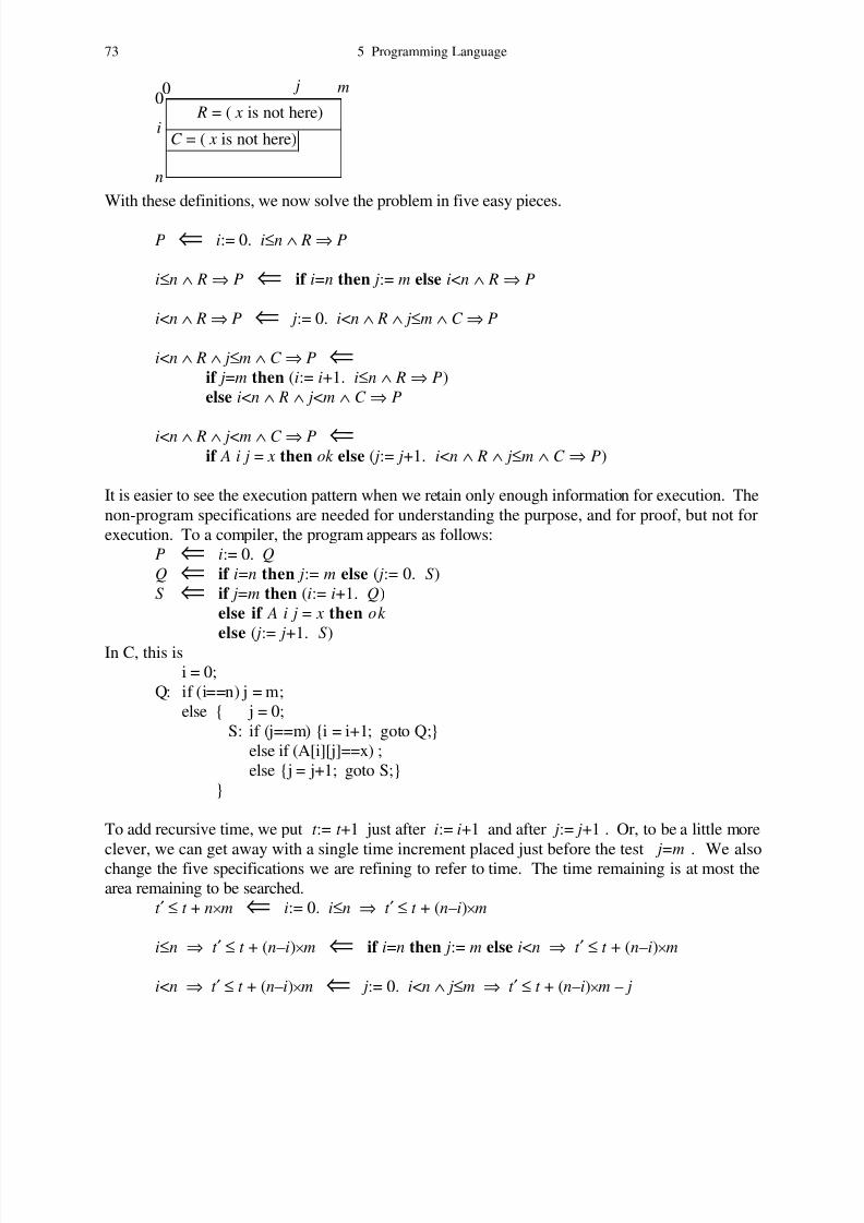
8/8/2019 37997710 Hehner a Practical Theory of Programming 2004
http://slidepdf.com/reader/full/37997710-hehner-a-practical-theory-of-programming-2004 80/242
C = ( x is not here)
R = ( x is not here)00
n
m
i
j
With these definitions, we now solve the problem in five easy pieces.
P ⇐ i:= 0. i≤n ∧ R ⇒ P
i≤n ∧ R ⇒ P ⇐ if i=n then j:= m else i<n ∧ R ⇒ P
i<n ∧ R ⇒ P ⇐ j:= 0. i<n ∧ R ∧ j≤m ∧ C ⇒ P
i<n ∧ R ∧ j≤m ∧ C ⇒ P ⇐if j=m then (i:= i+1. i≤n ∧ R ⇒ P)
else i<n ∧ R ∧ j<m ∧ C ⇒ P
i<n ∧ R ∧ j<m ∧ C ⇒ P ⇐if A i j = x then ok else ( j:= j+1. i<n ∧ R ∧ j≤m ∧ C ⇒ P)
It is easier to see the execution pattern when we retain only enough information for execution. The
non-program specifications are needed for understanding the purpose, and for proof, but not for
execution. To a compiler, the program appears as follows:
P ⇐ i:= 0. Q
Q ⇐ if i=n then j:= m else ( j:= 0. S)
S ⇐ if j=m then (i:= i+1. Q)
else if A i j = x then ok
else ( j:= j+1. S)
In C, this is
i = 0;
Q: if (i==n) j = m;
else { j = 0;
S: if (j==m) {i = i+1; goto Q;}
else if (A[i][j]==x) ;
else {j = j+1; goto S;}
}
To add recursive time, we put t := t +1 just after i:= i+1 and after j:= j+1 . Or, to be a little more
clever, we can get away with a single time increment placed just before the test j=m . We alsochange the five specifications we are refining to refer to time. The time remaining is at most the
area remaining to be searched.
t ′ ≤ t + n×m ⇐ i:= 0. i≤n ⇒ t ′ ≤ t + (n–i)×m
i≤n ⇒ t ′ ≤ t + (n–i)×m ⇐ if i=n then j:= m else i<n ⇒ t ′ ≤ t + (n–i)×m
i<n ⇒ t ′ ≤ t + (n–i)×m ⇐ j:= 0. i<n ∧ j≤m ⇒ t ′ ≤ t + (n–i)×m – j
73 5 Programming Language

8/8/2019 37997710 Hehner a Practical Theory of Programming 2004
http://slidepdf.com/reader/full/37997710-hehner-a-practical-theory-of-programming-2004 81/242
i<n ∧ j≤m ⇒ t ′ ≤ t + (n–i)×m – j ⇐t := t +1.
if j=m then (i:= i+1. i≤n ⇒ t ′ ≤ t + (n–i)×m)
else i<n ∧ j<m ⇒ t ′ ≤ t + (n–i)×m – j
i<n ∧ j<m ⇒ t ′ ≤ t + (n–i)×m – j ⇐if A i j = x then ok
else ( j:= j+1. i<n ∧ j≤m ⇒ t ′ ≤ t + (n–i)×m – j)
End of Two-Dimensional Search
5.2.3 For Loop
Let us use the syntax
for i:= m;..n do P
where i is a fresh name, m and n are integer expressions such that m ≤n , and P is a
specification, as an almost-typical notation for controlled iteration. The difference from popular
languages is just that iteration continues up to but excluding i=n . To avoid some thorns, let us
say also that i is not a state variable (so it cannot be assigned within P ), and that the initial valuesof m and n control the iteration.
As with the previous loop constructs, we will not equate the for-loop to a boolean expression, but
instead show how it is used in refinement. Let F be a function of two integer variables whose
result is a specification such that
Fmn ⇐ m=n ∧ ok
Fik ⇐ m≤i< j<k ≤n ∧ (Fij. Fjk )
Then
Fmn ⇐ for i:= m;..n do m≤i<n ⇒ Fi(i+1)
So Fmn is refined by a for-loop whose index runs from (including) m to (excluding) n . If
m=n there are no iterations, and specification Fmn must be satisfied by doing nothing. It alsomust be satisfied by first doing the iterations from m to an intermediate index j , and then doing
the rest of the iterations from j to n . The body of the loop has to do one iteration; the antecedent
of the body m≤i<n is optional.
For example, let the state consist of integer variable x , and let F be defined as
F = λi, j: nat · x′ = x×2 j–i
Then we can solve the exponentiation problem x′=2n in three refinements:
x′=2n ⇐ x:= 1. F 0n
F 0n ⇐ for i:= 0;..n do Fi(i+1)
Fi(i+1) ⇐ x:= 2× x
The recursive time measure requires each loop to contain a time increment of at least one time unit.
In general, the time taken by the body of a for loop may be a function f of the iteration i . Using
t ′ = t + Σi: m,..n· fi as for-loop specification Fmn , the for-loop rule tells us
t ′ = t + Σi: m,..n· fi ⇐ for i:= m;..n do t ′ = t + fi
When the body takes constant time c , this simplifies to
t ′ = t + (n–m)×c ⇐ for i:= m;..n do t ′ = t +c
A typical use of the for-loop rule is to do something to each item in a list. For example, Exercise
268 asks us to add 1 to each item in a list. The specification is
# L′=# L ∧ ∀i: 0,..# L· L′i= Li+1
5 Programming Language 74

8/8/2019 37997710 Hehner a Practical Theory of Programming 2004
http://slidepdf.com/reader/full/37997710-hehner-a-practical-theory-of-programming-2004 82/242
Now we need a specification Fik that describes an arbitrary segment of iterations: adding 1 to
each item from index i to index k .
Fik = # L′=# L ∧ (∀ j: i,..k · L′ j= Lj+1) ∧ (∀ j: (0,..i), (k ,..# L)· L′ j= Lj)
We check both
F 0 (# L) ⇐ 0=# L ∧ ok
Fik ⇐ 0≤i< j<k ≤# L ∧ (Fij. Fjk )
and find them to be theorems. So that gives us
F 0 (# L) ⇐ for i:= 0;..# L do Fi(i+1)
Now all we need is a refinement for Fi(i+1) .
Fi(i+1) ⇐ L:= i→ Li+1 | L
Sometimes the for-loop specification Fmn has the form Im⇒ I ′n , where I is a function of one
variable whose result is a precondition, and I ′ is the function whose result is the corresponding
postcondition. When I is applied to the for-loop index, condition Ii is called an invariant. An
advantage of this form of specification is that both Fii ⇐ ok and Fik ⇐ (Fij. Fjk ) are
automatically satisfied. Not all for-loop specifications can be put in this form; neither the timing
nor the previous example (add 1 to each item) can be. But the earlier exponential example can be
put in this form. Define I = λi: nat · x=2i
Then the solution is
x′=2n ⇐ x:= 1. I 0⇒ I ′n I 0⇒ I ′n ⇐ for i:= 0;..n do Ii⇒ I ′(i+1)
Ii⇒ I ′(i+1) ⇐ x:= 2× x
As another example of the invariant form of the for-loop rule, here is Exercise 186(a): Given a list
of integers, possibly including negatives, write a program to find the minimum sum of any
segment (sublist of consecutive items). Let L be the list. Formally, the problem is P where
P = s′ = MIN i, j· Σ L [i;.. j]
where 0 ≤ i ≤ j ≤ # L . The condition I k will say that s is the minimum sum of any segment upto index k . For k =0 there is only one segment, the empty segment, and its sum is 0 . When
k =# L all segments are included and we have the desired result. To go from I k to I (k +1) we
have to consider those segments that end at index k +1 . We could find the sum of each new
segment, then take the minimum of those sums and of s to be the new value of s . But we can do
better. Each segment ending at index k +1 is a one-item extension of a segment ending at index k
with one exception: the empty segment ending at k +1 .
[ 4 ; –2 ; –8 ; 7 ; 3 ; 0 ; –1 ]
k k +1
If we know the minimum sum c of any segment ending at k , then min (c + L k ) 0 is the
minimum sum of any segment ending at k +1 . So we define, for 0 ≤ k ≤ # L ,
I k = s = ( MIN i: 0,..k +1· MIN j: i,..k +1· Σ L [i;.. j])
∧ c = ( MIN i: 0,..k +1· Σ L [i;..k ])
Now the program is easy.
P ⇐ s:= 0. c:= 0. I 0 ⇒ I ′(# L)
I 0 ⇒ I ′(# L) ⇐ for k := 0;..# L do I k ⇒ I ′(k +1)
I k ⇒ I ′(k +1) ⇐ c:= min (c + L k ) 0. s:= min c s
End of For Loop
75 5 Programming Language

8/8/2019 37997710 Hehner a Practical Theory of Programming 2004
http://slidepdf.com/reader/full/37997710-hehner-a-practical-theory-of-programming-2004 83/242
5.2.4 Go To
For every set of loop constructs, there is some pattern of execution that cannot be conveniently
expressed using them. For that reason, many languages include a loop-building primitive: the
goto . Programming texts often warn that the go to is harmful, and should be avoided,
without saying why. The trouble with go to is that it cannot be considered a specification, and it
does not refine any specification. It does not fit in any usable theory of programming. If you are
not using any theory of programming, and your only understanding of programs is the ability to
execute them, there is no reason to avoid go to .
Refinement is more than any set of loop constructs; it provides not only tail recursions (branching)
but also general recursions (stacking). It provides all possible patterns of execution. Its closest
relative in many popular programming languages is the procedure declaration and call, but
unfortunately the refinement aspect is usually coupled with parameterization and local scope
aspects, and the implementation is often poor. For efficient execution, it may be necessary to code
the refinements using the execution-control primitives, such as go to , that are provided in an
available programming language.
End of Go To End of Control Structures
5.3 Time and Space Dependence
Some programming languages provide a clock, or a delay, or other time-dependent features. Our
examples have used the time variable as a ghost, or auxiliary variable, never affecting the course of
a computation. It was used as part of the theory, to prove something about the execution time.
Used for that purpose only, it did not need representation in a computer. But if there is a readable
clock available as a time source during a computation, it can be used to affect the computation. The
assignment deadline:= t + 5 is allowed, as is if t ≤ deadline then ... else ... . But the
assignment t := 5 is not allowed. We can look at the clock, but not reset it arbitrarily; all clock changes must correspond to the passage of time (according to some measure). (A computer
operator may need to set the clock sometimes, but that is not part of the theory of programming.)
We may occasionally want to specify the passage of time. For example, we may want the
computation to “wait until time w ”. Let us invent a notation for it, and define it formally as
wait until w = t := max t w
Because we are not allowed to reset the clock, t := max t w is not acceptable as a program until we
refine it. Letting time be an extended integer and using recursive time,
wait until w ⇐ if t ≥w then ok else (t := t +1. wait until w)
and we obtain a busy-wait loop. We can prove this refinement by cases. First,
t ≥w ∧ ok = t ≥w ∧ (t := t )
⇒ t := max t w
And second,
t <w ∧ (t := t +1. t := max t w)
In the left conjunct, use t : xint . In the right conjunct, use the Substitution Law.
= t +1 ≤ w ∧ (t := max (t +1) w)
= t +1 ≤ w ∧ (t := w)
= t <w ∧ (t := max t w)
⇒ t := max t w
5 Programming Language 76

8/8/2019 37997710 Hehner a Practical Theory of Programming 2004
http://slidepdf.com/reader/full/37997710-hehner-a-practical-theory-of-programming-2004 84/242
In programs that depend upon time, we should use the real time measure, rather than the recursive
time measure. We also need to be more careful where we place our time increments. And we need
a slightly different definition of wait until w , but we leave that as Exercise 275(b).
Our space variable s , like the time variable t , has so far been used to prove things about space
usage, not to affect the computation. But if a program has space usage information available to it,
there is no harm in using that information. Like t , s can be read but not written arbitrarily. All
changes to s must correspond to changes in space usage.
End of Time and Space Dependence
5.4 Assertions optional
5.4.0 Checking
As a safety check, some programming languages include the notation
assert b
where b is boolean. It is executed by checking that b is true; if it is, execution continues
normally, but if not, an error message is printed and execution is suspended. The intention is thatin a correct program, the asserted expressions will always be true, and so all assertions are
redundant. All error checking requires redundancy, and assertions help us to find errors and
prevent subsequent damage to the state variables.
Assertions are defined as follows.
assert b = if b then ok else ( print "error". wait until ∞)
If b is true, assert b is the same as ok . If b is false, execution cannot proceed in finite time to
any following actions. Assertions are an easy way to make programs more robust.
End of Checking
5.4.1 Backtracking
If P and Q are implementable specifications, so is P∨Q . The disjunction can be implemented
by choosing one of P or Q and satisfying it. Normally this choice is made as a refinement,
either P∨Q ⇐ P or P∨Q ⇐ Q . We could save this programming step by making disjunction a
programming connective, perhaps using the notation or . For example,
x:= 0 or x:= 1
would be a program whose execution assigns either 0 or 1 to x . This would leave the choice of
disjunct to the programming language implementer.
The next construct radically changes the way we program. We introduce the notation
ensure bwhere b is boolean, and define it as follows.
ensure b = if b then ok else
= b ∧ ok
Like assert b , ensure b is equal to ok if b is true. But when b is false, there is a problem:
it is unsatisfiable. By itself, this construct is unimplementable (unless b is identically true).
However, in combination with other constructs, the whole may be implementable. Consider the
following example in variables x and y .
77 5 Programming Language

8/8/2019 37997710 Hehner a Practical Theory of Programming 2004
http://slidepdf.com/reader/full/37997710-hehner-a-practical-theory-of-programming-2004 85/242
x:= 0 or x:= 1. ensure x=1
= ∃ x′′, y′′· ( x′′=0 ∧ y′′= y ∨ x′′=1 ∧ y′′= y) ∧ x′′=1 ∧ x′= x′′ ∧ y′= y′′
= x′=1 ∧ y′= y
= x:= 1
Although an implementation is given a choice between x:= 0 and x:= 1 , it must choose the right
one to satisfy a later condition. It can do so by making either choice (as usual), and when faced
with a later ensure whose condition is false, it must backtrack and make another choice. Since
choices can be nested within choices, a lot of bookkeeping is necessary.
Several popular programming languages, such as Prolog, feature backtracking. They may state
that choices are made in a particular order (we have omitted that complication). Two warnings
should accompany such languages. First, it is the programmer's responsibility to show that a
program is implementable; the language does not guarantee it. Alternatively, the implementation
does not guarantee that computations will satisfy the program, since it is sometimes impossible to
satisfy it. The second warning is that the time and space calculations do not work.
End of Backtracking
End of Assertions
5.5 Subprograms
5.5.0 Result Expression
Let P be a specification and e be an expression in unprimed variables. Then
P result e
is an expression of the initial state. It expresses the result of executing P and then evaluating e .
For example, the following expresses an approximation to the base of the natural logarithms.
var term, sum: rat := 1·
for i:= 1;..15 do (term:= term / i. sum:= sum+term)
result sumThe axiom for the result expression is
x′ = (P result e) = P. x′=e
where x is any state variable of the right type.
The example introduces local variables term and sum , and no other variables are reassigned. So
clearly the nonlocal state is unchanged. But consider
y:= y+1 result y
The result is as if the assignment y:= y+1 were executed, then y is the result, except that the
value of variable y is unchanged.
x:= ( y:= y+1 result y)
= x′ = ( y:= y+1 result y) ∧ y′= y= ( y:= y+1. x′= y) ∧ y′= y
= x′ = y+1 ∧ y′= y
= x:= y+1
When nonlocal variables seem to be changed (but they really aren't), implementation of result
expressions presents a difficulty, although not an impossibility. To avoid the difficulty, we have a
choice: we can forbid assignments to nonlocal variables within result expressions, or we can
allow nonlocal variables to change with a warning that mathematical reasoning is no longer
possible. For example, we cannot say x+ x = 2× x , nor even x= x , since x might be defined as
x = ( y:= y+1 result y)
5 Programming Language 78
8/8/2019 37997710 Hehner a Practical Theory of Programming 2004
http://slidepdf.com/reader/full/37997710-hehner-a-practical-theory-of-programming-2004 86/242
State changes resulting from the evaluation of an expression are called “side-effects”. If side-
effects are allowed, we have to get rid of result expressions before using any theory. For
example,
x:= (P result e) becomes (P. x:= e)
after renaming local variables within P as necessary to avoid clashes with nonlocal variables, and
allowing the scope of variables declared in P to extend through x:= e . For another example,
x:= y + (P result e) becomes (var z:= y· P. x:= z+e)
with similar provisos.
The recursive time measure that we have been using neglects the time for expression evaluation.
This is reasonable in some applications for expressions consisting of a few operations implemented
in computer hardware. For expressions using operations not implemented in hardware (perhaps
list catenation) it is questionable. For result expressions containing loops, it is unreasonable. We
must find a time bound for the program part, and charge that much time.
End of Result Expression
5.5.1 Function
In many popular programming languages, a function is a combination of assertion about the result,
name of the function, parameters, scope control, and result expression. It's a “package deal”.
For example, in C, the binary exponential function looks like this:
int bexp (int n)
{ int r = 1;
int i;
for (i=0; i<n; i++) r = r*2;
result r; }
In our notations, this would be
bexp = λn: int ·
( var r : int := 1·for i:= 0;..n do r := r ×2.
assert r : int
result r )
We present these programming features separately so that they can be understood separately. They
can be combined in any way desired, as in the example. The harm in providing one construct for
the combination is its complexity. Programmers trained with these languages may be unable to
separate the issues and realize that naming, parameterization, assertions, local scope, and result
expressions are independently useful.
Even the form of function we are using in this book could be both simplified and generalized.
Stating the domain of a parameter is a special case of axiom introduction, which can be separatedfrom name introduction (see Exercise 90).
End of Function
79 5 Programming Language
8/8/2019 37997710 Hehner a Practical Theory of Programming 2004
http://slidepdf.com/reader/full/37997710-hehner-a-practical-theory-of-programming-2004 87/242
5.5.2 Procedure
The procedure (or void function, or method), as it is found in many languages, is a “package deal”
like the function. It combines name declaration, parameterization, and local scope. The comments
of the previous subsection apply here too. There are also some new issues.
To use our theory for program development, not just verification, we must be able to talk about a
procedure whose body is an unrefined specification, not yet a program. For example, we may
want a procedure P with parameter x defined as
P = λ x: int · a′ < x < b′
that assigns variables a and b values that lie on opposite sides of a value to be supplied as
argument. We can use procedure P before we refine its body. For example,
P 3 = a′ < 3 < b′P (a+1) = a′ < a+1 < b′
The body is easily refined as
a′ < x < b′ ⇐ a:= x–1. b:= x+1
Our choice of refinement does not alter our definition of P ; it is of no use when we are using P .
A procedure and argument can be translated to a local variable and initial value.
(λ p: D· B) a = (var p: D := a· B)
This translation suggests that a parameter is really just a local variable whose initial value will be
supplied as an argument. In many popular programming languages, that is exactly the case. This
is an unfortunate confusion of specification and implementation. The decision to create a
parameter, and the choice of its domain, are part of a procedural specification, and are of interest to
a user of the procedure. The decision to create a local variable, and the choice of its domain, are
normally part of refinement, part of the process of implementation, and should not be of concern to
a user of the procedure. When a parameter is assigned a value within a procedure body, it is acting
as a local variable and no longer has any connection to its former role as parameter.
Another kind of parameter, usually called a reference parameter or var parameter, does not act as a
local variable, but stands for an unknown nonlocal variable to be supplied as argument. Here is an
example, using λ* to introduce a reference parameter.
(λ* x: int · x:= 3. b:= a) a = a:= 3. b:= a = a′ = b′ = 3
Formally, a reference parameter is two parameters, one for the initial value and one for the final
value, and the argument is correspondingly two arguments.
(λ* p: D· B) a = (λ p, p′: D· B) a a′Unfortunately, the arguments must be substituted for the parameters before any other
manipulations are performed. We are prevented from manipulating the procedure body by itself,
and must apply our programming theory separately for each call. In our example, we cannot say
whether x:= 3. b:= a = b:= a. x:= 3
without seeing the argument for parameter x . To a large degree, this contradicts the purpose of a
procedure.
End of Procedure
End of Subprograms
5 Programming Language 80
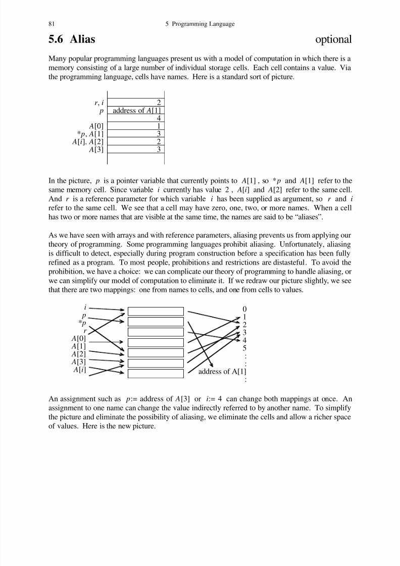
8/8/2019 37997710 Hehner a Practical Theory of Programming 2004
http://slidepdf.com/reader/full/37997710-hehner-a-practical-theory-of-programming-2004 88/242
5.6 Alias optional
Many popular programming languages present us with a model of computation in which there is a
memory consisting of a large number of individual storage cells. Each cell contains a value. Via
the programming language, cells have names. Here is a standard sort of picture.
r , i 2 p address of A[1]
4 A[0] 1
* p, A[1] 3 A[i], A[2] 2
A[3] 3
In the picture, p is a pointer variable that currently points to A[1] , so * p and A[1] refer to the
same memory cell. Since variable i currently has value 2 , A[i] and A[2] refer to the same cell.
And r is a reference parameter for which variable i has been supplied as argument, so r and i refer to the same cell. We see that a cell may have zero, one, two, or more names. When a cell
has two or more names that are visible at the same time, the names are said to be “aliases”.
As we have seen with arrays and with reference parameters, aliasing prevents us from applying our
theory of programming. Some programming languages prohibit aliasing. Unfortunately, aliasing
is difficult to detect, especially during program construction before a specification has been fully
refined as a program. To most people, prohibitions and restrictions are distasteful. To avoid the
prohibition, we have a choice: we can complicate our theory of programming to handle aliasing, or
we can simplify our model of computation to eliminate it. If we redraw our picture slightly, we see
that there are two mappings: one from names to cells, and one from cells to values.
i p* p
r A[0] A[1] A[2] A[3] A[i]
012345::
address of A[1]:
An assignment such as p:= address of A[3] or i:= 4 can change both mappings at once. Anassignment to one name can change the value indirectly referred to by another name. To simplify
the picture and eliminate the possibility of aliasing, we eliminate the cells and allow a richer space
of values. Here is the new picture.
81 5 Programming Language
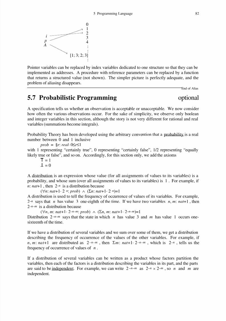
8/8/2019 37997710 Hehner a Practical Theory of Programming 2004
http://slidepdf.com/reader/full/37997710-hehner-a-practical-theory-of-programming-2004 89/242
i p A
01234::
[1; 3; 2; 3]:
Pointer variables can be replaced by index variables dedicated to one structure so that they can be
implemented as addresses. A procedure with reference parameters can be replaced by a function
that returns a structured value (not shown). The simpler picture is perfectly adequate, and the
problem of aliasing disappears.
End of Alias
5.7 Probabilistic Programming optional
A specification tells us whether an observation is acceptable or unacceptable. We now consider
how often the various observations occur. For the sake of simplicity, we observe only booleanand integer variables in this section, although the story is not very different for rational and real
variables (summations become integrals).
Probability Theory has been developed using the arbitrary convention that a probability is a real
number between 0 and 1 inclusive
prob = §r : real· 0≤r ≤1
with 1 representing “certainly true”, 0 representing “certainly false”, 1/2 representing “equally
likely true or false”, and so on. Accordingly, for this section only, we add the axioms
= 1
= 0
A distribution is an expression whose value (for all assignments of values to its variables) is a
probability, and whose sum (over all assignments of values to its variables) is 1 . For example, if
n: nat +1 , then 2–n is a distribution because
(∀n: nat +1· 2–n: prob) ∧ (Σn: nat +1· 2–n)=1
A distribution is used to tell the frequency of occurrence of values of its variables. For example,
2–n says that n has value 3 one-eighth of the time. If we have two variables n, m: nat +1 , then
2–n–m is a distribution because
(∀n, m: nat +1· 2–n–m: prob) ∧ (Σn, m: nat +1· 2–n–m)=1
Distribution 2–n–m says that the state in which n has value 3 and m has value 1 occurs one-
sixteenth of the time.
If we have a distribution of several variables and we sum over some of them, we get a distribution
describing the frequency of occurrence of the values of the other variables. For example, if
n,m:nat +1 are distributed as 2–n–m , then Σm : nat +1· 2–n–m , which is 2–n , tells us the
frequency of occurrence of values of n .
If a distribution of several variables can be written as a product whose factors partition the
variables, then each of the factors is a distribution describing the variables in its part, and the parts
are said to be independent. For example, we can write 2–n–m as 2–n × 2–m , so n and m are
independent.
5 Programming Language 82

8/8/2019 37997710 Hehner a Practical Theory of Programming 2004
http://slidepdf.com/reader/full/37997710-hehner-a-practical-theory-of-programming-2004 90/242
The average value of number expression e as variables v vary over their domains according to
distribution p is
Σv· e × p
For example, the average value of n2 as n varies over nat +1 according to distribution 2–n is
Σn: nat +1· n2 × 2–n , which is 6 . The average value of n–m as n and m vary over nat +1
according to distribution 2–n–m is Σn, m: nat +1· (n–m) × 2–n–m , which is 0 .
Let S be an implementable deterministic specification. Let p be the distribution describing the
initial state σ . Then the distribution describing the final state σ′ is
Σσ · S × p
which is a generalization of the formula for average. Here is an example in two integer variables x
and y . Suppose x starts with value 7 one-third of the time, and starts with value 8 two-thirds
of the time. Then the distribution of x is
( x=7) × 1/3 + ( x=8) × 2/3
The probability that x has value 7 is therefore
(7=7) × 1/3 + (7=8) × 2/3
= × 1/3 + × 2/3
= 1 × 1/3 + 0 × 2/3= 1/3
Similarly, the probability that x has value 8 is 2/3 , and the probability that x has value 9 is
0. Let X be the preceding distribution of x . Suppose that y also starts with value 7 one-
third of the time, and starts with value 8 two-thirds of the time, independently of x . Then its
distribution Y is given by
Y = ( y=7) / 3 + ( y=8) × 2/3
and the distribution of initial states is X × Y . Let S be
if x= y then ( x:= 0. y:= 0) else ( x:= abs( x– y). y:= 1)
Then the distribution of final states is
Σ x, y· S × X × Y
= Σ x, y· ( x= y ∧ x′= y′=0 ∨ x y ∧ x′=abs( x– y) ∧ y′=1)× (( x=7) / 3 + ( x=8) × 2/3)
× (( y=7) / 3 + ( y=8) × 2/3)
= ( x′= y′=0) × 5/9 + ( x′= y′=1) × 4/9
We should see x′= y′=0 five-ninths of the time, and x′= y′=1 four-ninths of the time.
Suppose we have one natural variable n . The specification ok is not a distribution of n and n′ because there are many pairs of values that give n′=n the value or 1 , and
Σn, n′· n′=n = ∞But
Σn′· n′=n = 1
so for any fixed value of n , ok is a distribution of n′ , telling us that n′ always has the valuen. Similary n′=n+1 is a distribution telling us that, for any given initial value of n , n′ always
has the value n+1 . An implementable deterministic specification is a distribution of the final state.
Suppose we have one natural variable n whose initial value is 5 . After executing the
nondeterministic specification ok ∨ (n:= n+1) , we can say that the final value of n is either 5 or
6 . Now suppose this specification is executed many times, and the distribution of initial states is
n=5 ( n always starts with value 5 ). What is the distribution of final states? Nondeterminism is
a freedom for the implementer, who may refine the specification as ok , which always gives the
answer n′=5 , or as n:= n+1 , which always gives the answer n′=6 , or as
if event then ok else n:= n+1
83 5 Programming Language

8/8/2019 37997710 Hehner a Practical Theory of Programming 2004
http://slidepdf.com/reader/full/37997710-hehner-a-practical-theory-of-programming-2004 91/242
which gives n′=5 or n′=6 unpredictably. In general, we cannot say the distribution of final
states after a nondeterministic specification. If we apply the formula Σσ· S × p to a specification
S that is unimplementable or nondeterministic, the result may not be a distribution. For example,
the nondeterministic specification ok ∨ (n:= n+1) is not a distribution, not even when the initial
value of n is fixed, because
Σn′· ok ∨ (n:= n+1) = 2
which is the degree of nondeterminism. Nondeterministic choice is equivalent to deterministic
choice in which the determining expression is a variable of unknown value.
P ∨ Q = ∃b: bool· if b then P else Q
Thus we can always eliminate nondeterminism by introducing a new variable.
We now generalize conditional composition and dependent composition to apply to probabilistic
specifications as follows. If b is a probability, and P and Q are distributions of final states,
if b then P else Q = b × P + (1–b) × Q
P.Q = Σσ′′· (substitute σ′′ for σ′ in P ) × (substitute σ′′ for σ in Q )
are distributions of final states. For example, in one integer variable x , suppose we start by
assigning 0 with probability 1/3 or 1 with probability 2/3 ; that's
if 1/3 then x:= 0 else x:= 1Subsequently, if x=0 then we add 2 with probability 1/2 or 3 with probability 1/2 , otherwise
we add 4 with probability 1/4 or 5 with probability 3/4 ; that's
if x=0 then if 1/2 then x:= x+2 else x:= x+3 else if 1/4 then x:= x+4 else x:= x+5
Notice that the programmer's if gives us conditional probability. Our calculation
if 1/3 then x:= 0 else x:= 1.
if x=0 then if 1/2 then x:= x+2 else x:= x+3
else if 1/4 then x:= x+4 else x:= x+5
= Σ x′′· (( x′′=0)/3 + ( x′′=1)×2/3)
× ( ( x′′=0) × (( x′= x′′+2)/2 + ( x′= x′′+3)/2)
+ ( x′′ 0) × (( x′= x′′+4)/4 + ( x′= x′′+5)×3/4))
= ( x′=2)/6 + ( x′=3)/6 + ( x′=5)/6 + ( x′=6)/2says that the result is 2 with probability 1/6 , 3 with probability 1/6 , 5 with probability 1/6 ,
and 6 with probability 1/2 .
We earlier used the formula Σ σ · S × p to calculate the distribution of final states from the
distribution p of initial states and an operation specified by S . We can now restate this formula
as ( p′. S) where p′ is the same as p but with primes on the variables.
Various distribution laws are provable from probabilistic sequential composition. Let n be a
number, and let P , Q , and R be probabilistic specifications. Then
n×P. Q = n×(P. Q) = P. n×Q
P+Q. R = (P. R) + (Q. R)P. Q+ R = (P. Q) + (P. R)
Best of all, the Substitution Law still works.
5.7.0 Random Number Generators
Many programming languages provide a random number generator (sometimes called a “pseudo-
random number generator”). The usual notation is functional, and the usual result is a value whose
distribution is uniform (constant) over a nonempty finite range. If n: nat +1 , we use the notation
rand n for a generator that produces natural numbers uniformly distributed over the range 0,..n .
So rand n has value r with probability (r : 0,..n) / n .
5 Programming Language 84

8/8/2019 37997710 Hehner a Practical Theory of Programming 2004
http://slidepdf.com/reader/full/37997710-hehner-a-practical-theory-of-programming-2004 92/242
Functional notation for a random number generator is inconsistent. Since x= x is a law, we
should be able to simplify rand n = rand n to , but we cannot because the two occurrences of
rand n might generate different numbers. Since x+ x = 2 × x is a law, we should be able to
simplify rand n + rand n to 2 × rand n , but we cannot. To restore consistency, we replace each
use of rand n with a fresh integer variable r whose value has probability (r : 0,..n) / n before we
do anything else. Or, if you prefer, we replace each use of rand n with a fresh variable r : 0,..n
whose value has probability 1/ n . (This is a mathematical variable, or in other words, a state
constant; there is no r ′ .) For example, in one state variable x ,
x:= rand 2. x:= x + rand 3 replace the two rand s with r and s
= Σr : 0,..2· Σs: 0,..3· ( x:= r . x:= x + s) × 1/2 × 1/3 Substitution Law
= Σr : 0,..2· Σs: 0,..3· ( x′ = r +s) / 6 sum
= (( x′ = 0+0) + ( x′ = 0+1) + ( x′ = 0+2) + ( x′ = 1+0) + ( x′ = 1+1) + ( x′ = 1+2)) / 6
= ( x′=0) / 6 + ( x′=1) / 3 + ( x′=2) / 3 + ( x′=3) / 6
which says that x′ is 0 one-sixth of the time, 1 one-third of the time, 2 one-third of the time,
and 3 one-sixth of the time.
Whenever rand occurs in the context of a simple equation, such as r = rand n , we don't need to
introduce a variable for it, since one is supplied. We just replace the deceptive equation with(r :0,..n) / n . For example, in one variable x ,
x:= rand 2. x:= x + rand 3 replace assignments
= ( x′: 0,..2)/2. ( x′: x+(0,..3))/3 dependent composition
= Σ x′′· ( x′′: 0,..2)/2 × ( x′: x′′+(0,..3))/3 sum
= 1/2 × ( x′: 0,..3)/3 + 1/2 × ( x′: 1,..4)/3
= ( x′=0) / 6 + ( x′=1) / 3 + ( x′=2) / 3 + ( x′=3) / 6
as before.
Although rand produces uniformly distributed natural numbers, it can be transformed into many
different distributions. We just saw that rand 2 + rand 3 has value n with distribution
(n=0∨n=3) / 6 + (n=1 ∨ n=2) / 3 . As another example, rand 8 < 3 has boolean value b withdistribution
Σr : 0,..8· (b = (r <3)) / 8
= (b= ) × 3/8 + (b= ) × 5/8
= 5/8 – b /4
which says that b is three-eighths of the time, and five-eighths of the time.
Exercise 281 is a simplified version of blackjack. You are dealt a card from a deck; its value is in
the range 1 through 13 inclusive. You may stop with just one card, or have a second card if you
want. Your object is to get a total as near as possible to 14 , but not over 14 . Your strategy is to
take a second card if the first is under 7 . Assuming each card value has equal probability
(actually, the second card drawn has a diminished probability of having the same value as the firstcard drawn, but let's ignore that complication), we represent a card as (rand 13) + 1 . In one
variable x , the game is
x:= (rand 13) + 1. if x<7 then x:= x + (rand 13) + 1 else ok
replace rand and ok
= ( x′: (0,..13)+1)/13. if x<7 then ( x′: x+(0,..13)+1)/13 else x′= x replace . and if
= Σ x′′· ( x′′: 1,..14)/13 × (( x′′<7)×( x′: x′′+1,.. x′′+14)/13 + ( x′′≥7)×( x′= x′′))by several omitted steps
= ((2≤ x′<7)×( x′–1) + (7≤ x′<14)×19 + (14≤ x′<20)×(20– x′)) / 169
85 5 Programming Language

8/8/2019 37997710 Hehner a Practical Theory of Programming 2004
http://slidepdf.com/reader/full/37997710-hehner-a-practical-theory-of-programming-2004 93/242
That is the distribution of x′ if we use the “under 7 ” strategy. We can similarly find the
distribution of x′ if we use the “under 8 ” strategy, or any other strategy. But which strategy is
best? To compare two strategies, we play both of them at once. Player x will play “under n ”
and player y will play “under n+1 ” using exactly the same cards c and d (the result would be
no different if they used different cards, but it would require more variables). Here is the new
game, followed by the condition that x wins:
c:= (rand 13) + 1. d := (rand 13) + 1.
if c < n then x:= c+d else x:= c. if c < n+1 then y:= c+d else y:= c.
y< x≤14 ∨ x≤14< y Replace rand and use the functional-imperative law twice.
= (c′: (0,..13)+1 ∧ d ′: (0,..13)+1 ∧ x′= x ∧ y′= y) / 13 / 13.
x:= if c < n then c+d else c. y:= if c < n+1 then c+d else c.
y< x≤14 ∨ x≤14< y Use the substitution law twice.
= (c′: (0,..13)+1 ∧ d ′: (0,..13)+1 ∧ x′= x ∧ y′= y) / 169.
(if c < n+1 then c+d else c) < (if c < n then c+d else c) ≤ 14
∨ (if c < n then c+d else c) ≤ 14 < (if c < n+1 then c+d else c)
= (c′: (0,..13)+1 ∧ d ′: (0,..13)+1 ∧ x′= x ∧ y′= y) / 169. c=n ∧ d >14–n
= Σc′′, d ′′, x′′, y′′·
(c′′: (0,..13)+1 ∧ d ′′: (0,..13)+1 ∧ x′′= x ∧ y′′= y) / 169 × (c′′=n ∧ d ′′>14–n)= Σd ′′: 1,..14· (d ′′>14–n)/169
= (n–1) / 169
The probability that x wins is (n–1) / 169 . By similar calculations we can find that the
probability that y wins is (14–n) / 169 , and the probability of a tie is 12/13 . For n<8 , “under
n+1 ” beats “under n ”. For n≥ 8 , “under n ” beats “under n+1 ”. So “under 8 ” beats both
“under 7 ” and “under 9 ”.
Exercise 282 asks: If you repeatedly throw a pair of six-sided dice until they are equal, how long
does it take? The program is
R ⇐ u:= (rand 6) + 1. v:= (rand 6) + 1. if u=v then ok else (t := t +1. R)
for an appropriate definition of R .
Each iteration, with probability 5/6 we keep going, and with probability 1/6 we stop. So we
offer the hypothesis that the execution time has the distribution
(t ′≥t ) × (5/6)t ′–t × 1/6
To prove it, let's start with the implementation.
u:= (rand 6) + 1. v:= (rand 6) + 1. replace rand and
if u=v then t ′=t else (t := t +1. (t ′≥t ) × (5/6)t ′–t × 1/6) Substitution Law
= ((u′: 1,..7) ∧ v′=v ∧ t ′=t )/6. (u′=u ∧ (v′: 1,..7) ∧ t ′=t )/6. replace first .
if u=v then t ′=t else (t ′≥t +1) × (5/6)t ′–t –1 / 6 and simplify
= ((u′: 1,..7) ∧ (v′: 1,..7) ∧ t ′=t )/36. replace remaining .
if u=v then t ′=t else (t ′≥t +1) × (5/6)t ′–t –1 / 6 and replace if = Σu′′, v′′: 1,..7· Σt ′′· (t ′′=t )/36 × ((u′′=v′′) × (t ′=t ′′)
+ (u′′ v′′) × (t ′≥t ′′+1) × (5/6)t ′–t ′′–1 / 6) sum
= 1/36 × (6 × (t ′=t ) + 30 × (t ′≥t +1) × (5/6)t ′–t –1 / 6) combine
= (t ′≥t ) × (5/6)t ′–t × 1/6
which is the probabilistic specification, and that completes the proof.
The average value of t ′ is
Σt ′· t ′ × (t ′≥t ) × (5/6)t ′–t × 1/6 = t +5
so on average it takes 5 additional throws of the dice to get an equal pair.
End of Random Number Generators
5 Programming Language 86

8/8/2019 37997710 Hehner a Practical Theory of Programming 2004
http://slidepdf.com/reader/full/37997710-hehner-a-practical-theory-of-programming-2004 94/242
Probability problems are notorious for misleading even professional mathematicians. Informal
reasoning to arrive at a probability distribution, as is standard in studies of probability, is essential
to forming a reasonable hypothesis. But hypotheses are sometimes wrong. We write the
hypothesis as a probabilistic specification, we refine it as a program, and we prove our refinements
exactly as we did with boolean specifications. Sometimes wrong hypotheses can be traced to a
wrong understanding of the problem. Formalization as a program makes one's understanding
clear. Proof shows that a hypothesized probability distribution is correct for the program.
Informal arguments are replaced by formal proof.
Probabilistic specifications can also be interpreted as “fuzzy” specifications. For example,
( x′=0)/3 + ( x′=1)×2/3 could mean that we will be one-third satisfied if the result x′ is 0 , two-
thirds satisfied if it is 1 , and completely unsatisfied if it is anything else.
5.7.1 Information optional
There is a close connection between information and probability. If a boolean expression has
probability p of being true, and you evaluate it, and it turns out to be true, then the amount of
information in bits that you have just learned is info p , defined asinfo p = – log p
where log is the binary (base 2 ) logarithm. For example, even (rand 8) has probability 1/2 of
being true. If we evaluate it and find that it is true, we have just learned
info (1/2) = – log (1/2) = log 2 = 1
bit of information; we have learned that the rightmost bit of the random number we were given is
0 . If we find that even (rand 8) is false, then we have learned that ¬ even (rand 8) is true, and
since it also has probability 1/2 , we have also gained one bit; we have learned that the rightmost
bit of the random number is 1 . If we test rand 8 = 5 , which has probability 1/8 of being true,
and we find that it is true, we learn
info (1/8) = – log (1/8) = log 8 = 3
bits, which is the entire random number in binary. If we find that rand 8 = 5 is false, we learninfo (7/8) = – log (7/8) = log 8 – log 7 = 3 – 2.80736 = 0.19264 approximately
bits; we learn that the random number isn't 5 , but it could be any of 7 others. Suppose we test
rand 8 < 8 . Since it is certain to be true, there is really no point in making this test; we learn
info 1 = – log 1 = –0 = 0
When an if b then P else Q occurs within a loop, b is tested repeatedly. Suppose b has
probability p of being true. When it is true, we learn info p bits, and this happens with
probability p . When it is false, we learn info (1– p) bits, and this happens with probability
(1– p) . The average amount of information gained, called the entropy, is
entro p = p × info p + (1– p) × info (1– p)
For example, entro (1/2) = 1 , and entro (1/8) = entro (7/8) = 0.54356 approximately. Sinceentro p is at its maximum when p=1/2 , we learn most on average, and make the most efficient
use of the test, if its probability is near 1/2 . For example, in the binary search problem of Chapter
4, we could have divided the remaining search interval anywhere, but for the best average
execution time, we split it into two parts having equal probabilities of finding the item we seek.
End of Information
End of Probabilistic Programming
87 5 Programming Language

8/8/2019 37997710 Hehner a Practical Theory of Programming 2004
http://slidepdf.com/reader/full/37997710-hehner-a-practical-theory-of-programming-2004 95/242
5.8 Functional Programming optional
Most of this book is about a kind of programming that is sometimes called “imperative”, which
means that a program describes a change of state (or “commands” a computer to change state in a
particular way). This section presents an alternative: a program is a function from its input to its
output. More generally, a specification is a function from possible inputs to desired outputs, and
programs (as always) are implemented specifications. We take away assignment and dependent
composition from our programming notations, and we add functions.
To illustrate, we look once again at the list summation problem (Exercise 142). This time, the
specification is λ L: [*rat ]· Σ L . Assuming Σ is not an implemented operator, we still have some
programming to do. We introduce variable n to indicate how much of the list has been summed;
initially n is 0 .
Σ L = (λn: 0,..# L+1· Σ L [n;..# L]) 0
It saves some copying to write “ Σ L = ... ” rather than “ λ L: [*rat ]· Σ L = ... ”, but we must
remember the domain of L . At first sight, the domain of n is annoying; it seems to be one
occasion when an interval notation that includes both endpoints would be preferable. On second
look, it's trying to tell us something useful: the domain is really composed of two parts that mustbe treated differently.
0,..# L+1 = (0,..# L), # L
We divide the function into a selective union
λn: 0,..# L+1· Σ L [n;..# L] = (λn: 0,..# L· Σ L [n;..# L]) | (λn: # L· Σ L [n;..# L])
and continue with each part separately. In the left part, we have n < # L , and in the right part
n =# L .
λn: 0,..# L· Σ L [n;..# L] = λn: 0,..# L· Ln + Σ L [n+1;..# L]
λn: # L· Σ L [n;..# L] = λn: # L· 0
This time we copied the domain of n to indicate which part of the selective union is being
considered. The one remaining problem is solved by recursion.
Σ L [n+1;..# L] = (λn: 0,..# L+1· Σ L [n;..# L]) (n+1)
In place of the selective union we could have used if then else ; they are related by the law
(λv: A· x) | (λv: B· y) = λv: A, B· if v: A then x else y
When we are interested in the execution time rather than the result, we replace the result of each
function with its time according to some measure. For example, in the list summation problem, we
might decide to charge time 1 for each addition and 0 for everything else. The specification
becomes λ L: [*rat ]· # L , meaning for any list, the execution time is its length. We now must
make exactly the same programming steps as before. The first step was to introduce variable n ;
we do the same now, but we choose a new result for the new function to indicate its execution
time.# L = (λn: 0,..# L+1· # L–n) 0
The second step was to decompose the function into a selective union; we do so again.
λn: 0,..# L+1· # L–n = (λn: 0,..# L· # L–n) | (λn: # L· # L–n)
The left side of the selective union became a function with one addition in it, so our timing function
must become a function with a charge of 1 in it. To make the equation correct, the time for the
remaining summation must be adjusted.
λn: 0,..# L· # L–n = λn: 0,..# L· 1 + # L–n–1
The right side of the selective union became a function with a constant result; according to our
measure, its time must be 0 .
λn: # L· # L–n = λn: # L· 0
5 Programming Language 88

8/8/2019 37997710 Hehner a Practical Theory of Programming 2004
http://slidepdf.com/reader/full/37997710-hehner-a-practical-theory-of-programming-2004 96/242
The remaining problem was solved by a recursive call; the corresponding call solves the remaining
time problem.
# L–n–1 = (λn: 0,..# L+1· # L–n) (n+1)
And that completes the proof that execution time (according to this measure) is the length of the
list.
In the recursive time measure, we charge nothing for any operation except recursive call, and we
charge 1 for that. Let's redo the timing proof with this measure. Again, the time specification is
λ L: [*rat ]· # L .
# L = (λn: 0,..# L+1· # L–n) 0
λn: 0,..# L+1· # L–n = (λn: 0,..# L· # L–n) | (λn: # L· # L–n)
λn: 0,..# L· # L–n = λn: 0,..# L· # L–n
λn: # L· # L–n = λn: # L· 0
# L–n = 1 + (λn: 0,..# L+1· # L–n) (n+1)
5.8.0 Function Refinement
In imperative programming, we can write a nondeterministic specification such as x′: 2, 3, 4 thatallows the result to be any one of several possibilities. In functional programming, a
nondeterministic specification is a bunch consisting of more than one element. The specification
2, 3, 4 allows the result to be any one of those three numbers.
Functional specifications can be classified the same way as imperative specifications, based on the
number of satisfactory outputs for each input.
Functional specification S is unsatisfiable for domain element x : ¢ Sx = 0
Functional specification S is satisfiable for domain element x : ¢ Sx > 0
Functional specification S is deterministic for domain element x : ¢ Sx ≤ 1
Functional specification S is nondeterministic for domain element x : ¢ Sx > 1
Functional specification S is satisfiable for domain element x : ∃ y· y: Sx
Functional specification S is implementable: ∀ x· ∃ y· y: Sx
( x is quantified over the domain of S , and y is quantified over the range of S .)
Implementability can be restated as ∀ x· Sx null .
Consider the problem of searching for an item in a list of integers. Our first attempt at specification
might be
λ L: [*int ]· λ x: int · §n: 0,..# L· Ln = x
which says that for any list L and item x , we want an index of L where x occurs. If x occurs
several times in L , any of its indexes will do. Unfortunately, if x does not occur in L , we are
left without any possible result, so this specification is unimplementable. We must decide what wewant when x does not occur in L ; let's say any natural that is not an index of L will do.
λ L: [*int ]· λ x: int · if x: L (0,..# L) then §n: 0,..# L· Ln = x else # L,..∞This specification is implementable, and often nondeterministic.
Functional refinement is similar to imperative refinement. Functional specification P (the
problem) is refined by functional specification S (the solution) if and only if all results that are
satisfactory according to S are also satisfactory according to P . Formally, this is just inclusion
S: P . Now we have a most annoying notational problem. Typically, we like to write the problem
on the left, then the refinement symbol, then the solution on the right; we want to write S: P the
other way round. Inclusion is antisymmetric, so its symbol should not be symmetric, but
89 5 Programming Language

8/8/2019 37997710 Hehner a Practical Theory of Programming 2004
http://slidepdf.com/reader/full/37997710-hehner-a-practical-theory-of-programming-2004 97/242
unfortunately it is. Let us write :: for “backwards colon”, so that “ P is refined by S ” is written
P:: S .
To refine our search specification, we create a linear search program, starting the search with index
0 and increasing the index until either x is found or L is exhausted. First we introduce the
index.
(if x: L (0,..# L) then §n: 0,..# L· Ln = x else # L,..∞)::
(λi: nat · if x: L (i,..# L) then §n: i,..# L· Ln = x else # L,..∞) 0
The two sides of this refinement are equal, so we could have written = instead of :: . We could
have been more precise about the domain of i , and then we probably would decompose the
function into a selective union, as we did in the previous problem. But this time let's use an
ifthen else .
(if x: L (i,..# L) then §n: i,..# L· Ln = x else # L,..∞)::
if i = # L then # L
else if x = Li then i
else (λi· if x: L (i,..# L) then §n: i,..# L· Ln = x else # L,..∞) (i+1)
The timing specification, recursive measure, is λ L· λ x· 0,..# L+1 , which means that the time isless than # L+1 . To prove that this is the execution time, we must prove
0,..# L+1:: (λi· 0,..# L–i+1) 0
and
0,..# L–i+1:: if i = # L then 0
else if x = Li then 0
else 1 + (λi· 0,..# L–i+1) (i+1)
As this example illustrates, the steps in a functional refinement are the same as the steps in an
imperative refinement for the same problem, including the resolution of nondeterminism and
timing. But the notations are different.
End of Function Refinement
Functional and imperative programming are not really competitors; they can be used together. We
cannot ignore imperative programming if ever we want to pause, to stop computing for a while,
and resume later from the same state. Imperative programming languages all include a functional
(expression) sublanguage, so we cannot ignore functional programming either.
At the heart of functional programming we have the Application Axiom
(λv: D· b) x = (for v substitute x in b )
At the heart of imperative programming we have the Substitution Law
x:= e. P = (for x substitute e in P )
Functional programming and imperative programming differ mainly in the notation they use forsubstitution.
End of Functional Programming
End of Programming Language
5 Programming Language 90
8/8/2019 37997710 Hehner a Practical Theory of Programming 2004
http://slidepdf.com/reader/full/37997710-hehner-a-practical-theory-of-programming-2004 98/242
91
6 Recursive Definition
6.0 Recursive Data Definition
In this section we are concerned with the definition of infinite bunches. Our first example is nat ,
the natural numbers. It was defined in Chapter 2 using axioms called construction and induction.
Now we take a closer look at these axioms.
6.0.0 Construction and Induction
To define nat , we need to say what its elements are. We can start by saying that 0 is an element
0: nat
and then say that for every element of nat , adding 1 gives an element
nat +1: nat
These axioms are called the nat construction axioms, and 0 and nat +1 are called the nat
constructors. Using these axioms, we can “construct” the elements of nat as follows.
0: nat add 1 to each side
⇒ 0+1: nat +1 by arithmetic, 0+1 = 1 ; by the axiom, nat +1: nat ⇒ 1: nat add 1 to each side
⇒ 1+1: nat +1 by arithmetic, 1+1 = 2 ; by the axiom, nat +1: nat
⇒ 2: nat
and so on.
From the construction axioms we can prove 2: nat but we cannot prove ¬ –2: nat . That is why
we need the induction axiom. The construction axioms tell us that the natural numbers are in nat ,
and the induction axiom tells us that nothing else is. Here is the nat induction axiom.
0: B ∧ B+1: B ⇒ nat : B
We have introduced nat as a constant, like null and 0 . It is not a variable, and cannot be
instantiated. But B is a variable, to be instantiated at will.
The two construction axioms can be combined into one, and induction can be restated, as follows:
0, nat +1: nat nat construction
0, B+1: B ⇒ nat : B nat induction
There are many bunches satisfying the inclusion 0, B+1: B , such as: the naturals, the integers,
the integers and half-integers, the rationals. Induction says that of all these bunches, nat is the
smallest.
We have presented nat construction and nat induction using bunch notation. We now present
equivalent axioms using predicate notation. We begin with induction.
In predicate notation, the nat induction axiom can be stated as follows: If P: nat →bool ,
P0 ∧ ∀n: nat · Pn ⇒ P(n+1) ⇒ ∀n: nat · Pn
We prove first that the bunch form implies the predicate form.
0: B ∧ B+1: B ⇒ nat : B Let B = §n: nat · Pn . Then B: nat ,
⇒ 0: B ∧ (∀n: nat · n: B ⇒ n+1: B) ⇒ ∀n: nat · n: B and ∀n: nat · (n: B) = Pn .
= P0 ∧ (∀n: nat · Pn ⇒ P(n+1)) ⇒ ∀n: nat · Pn
8/8/2019 37997710 Hehner a Practical Theory of Programming 2004
http://slidepdf.com/reader/full/37997710-hehner-a-practical-theory-of-programming-2004 99/242
The reverse is proven similarly.
P0 ∧ (∀n: nat · Pn ⇒ P(n+1)) ⇒ ∀n: nat · Pn
For arbitrary bunch B , let P = λn: nat · n: B . Then again ∀n: nat · Pn = (n: B) .
⇒ 0: B ∧ (∀n: nat · n: B ⇒ n+1: B) ⇒ ∀n: nat · n: B
= 0: B ∧ (∀n: nat ‘ B· n+1: B) ⇒ ∀n: nat · n: B
= 0: B ∧ (nat ‘ B)+1: B ⇒ nat : B
⇒ 0: B ∧ B+1: B ⇒ nat : BTherefore the bunch and predicate forms of nat induction are equivalent.
The predicate form of nat construction can be stated as follows: If P: nat →bool ,
P0 ∧ ∀n: nat · Pn ⇒ P(n+1) ⇐ ∀n: nat · Pn
This is the same as induction but with the main implication reversed. We prove first that the bunch
form implies the predicate form.
∀n: nat · Pn domain change using nat construction, bunch version
⇒ ∀n: 0, nat +1· Pn axiom about ∀
= (∀n: 0· Pn) ∧ (∀n: nat +1· Pn) One-Point Law and variable change
= P0 ∧ ∀n: nat · P(n+1)
⇒ P0 ∧ ∀n: nat · Pn ⇒ P(n+1)And now we prove that the predicate form implies the bunch form .
P0 ∧ (∀n: nat · Pn ⇒ P(n+1)) ⇐ ∀n: nat · Pn Let P = λn: nat · n: nat
⇒ 0: nat ∧ (∀n: nat · n: nat ⇒ n+1: nat ) ⇐ ∀n: nat · n: nat
= 0: nat ∧ (∀n: nat · n+1: nat ) ⇐
= 0: nat ∧ nat +1: nat
A corollary is that nat can be defined by the single axiom
P0 ∧ ∀n: nat · Pn ⇒ P(n+1) = ∀n: nat · Pn
There are other predicate versions of induction; here is the usual one again plus three more.
P0 ∧ ∀n: nat · Pn ⇒ P(n+1) ⇒ ∀n: nat · Pn
P0 ∨ ∃n: nat · ¬Pn ∧ P(n+1) ⇐ ∃n: nat · Pn∀n: nat · Pn ⇒ P(n+1) ⇒ ∀n: nat · P0 ⇒ Pn
∃n: nat · ¬Pn ∧ P(n+1) ⇐ ∃n: nat · ¬P0 ∧ Pn
The first version says that to prove P of all naturals, prove it of 0 , and assuming it of natural n ,
prove it of n+1 . In other words, you get to all naturals by starting at 0 and repeatedly adding
1. The second version is obtained from the first by the duality laws and a renaming. The third is
the prettiest; it says that if you can “go” from any natural to the next, then you can “go” from 0 to
any natural.
Here are two laws that are consequences of induction.
∀n: nat · (∀m: nat · m<n ⇒ Pm) ⇒ Pn ⇒ ∀n: nat · Pn
∃n: nat · (∀m: nat · m<n ⇒ ¬Pm) ∧ Pn ⇐ ∃n: nat · PnThe first is like the first version of induction, except that the base case P0 is not explicitly stated,
and the step uses the assumption that all previous naturals satisfy P , rather than just the one
previous natural. The last one says that if there is a natural with property P then there is a first
natural with property P (all previous naturals don't have it).
6 Recursive Definition 92

8/8/2019 37997710 Hehner a Practical Theory of Programming 2004
http://slidepdf.com/reader/full/37997710-hehner-a-practical-theory-of-programming-2004 100/242
Proof by induction does not require any special notation or format. For example, Exercise 288
asks us to prove that the square of an odd natural number is 8×m + 1 for some natural m .
Quantifying over nat ,
∀n· ∃m· (2×n + 1)2 = 8×m + 1 various number laws
= ∀n· ∃m· 4×n×(n+1) + 1 = 8×m + 1 various number laws
= ∀n· ∃m· n×(n+1) = 2×m the usual predicate form of induction
⇐ (∃m· 0×(0+1) = 2×m) generalization and∧ (∀n· (∃m· n×(n+1) = 2×m) ⇒ (∃l· (n+1)×(n+2) = 2×l)) distribution
⇐ 0×(0+1) = 2×0 arithmetic and
∧ (∀n, m· n×(n+1) = 2×m ⇒ (∃l· (n+1)×(n+2) = 2×l)) generalization
⇐ ∀n, m· n×(n+1) = 2×m ⇒ (n+1)×(n+2) = 2×(m+n+1) various number laws
=
Now that we have an infinite bunch, it is easy to define others. For example, we can define pow
to be the powers of 2 either by the equation
pow = 2nat
or by using the solution quantifier
pow = § p: nat · ∃m: nat · p = 2mBut let us do it the same way we defined nat . The pow construction axiom is
1, 2× pow: pow
and the pow induction axiom is
1, 2× B: B ⇒ pow: B
Induction is not just for nat . In predicate form, we can define pow with the axiom
P1 ∧ ∀ p: pow· Pp ⇒ P(2× p) = ∀ p: pow· Pp
We can define the bunch of integers as
int = nat , –nat
or equivalently we can use the construction and induction axioms
0, int +1, int –1: int 0, B+1, B–1: B ⇒ int : B
or we can use the axiom
P0 ∧ (∀i: int · Pi ⇒ P(i+1)) ∧ (∀i: int · Pi ⇒ P(i–1)) = ∀i: int · Pi
Whichever we choose as axiom(s), the others are theorems.
Similarly we can define the bunch of rationals as
rat = int /(nat +1)
or equivalently by the construction and induction axioms
1, rat +rat , rat –rat , rat ×rat , rat /(§r : rat · r 0): rat
1, B+ B, B– B, B× B, B /(§b: B· b 0): B ⇒ rat : B
or with the axiom (quantifying over rat , of course) P1
∧ (∀r , s· Pr ∧ Ps ⇒ P(r +s))
∧ (∀r , s· Pr ∧ Ps ⇒ P(r –s))
∧ (∀r , s· Pr ∧ Ps ⇒ P(r ×s))
∧ (∀r , s· Pr ∧ Ps ∧ s 0 ⇒ P(r / s))
= ∀r · Pr
93 6 Recursive Definition

8/8/2019 37997710 Hehner a Practical Theory of Programming 2004
http://slidepdf.com/reader/full/37997710-hehner-a-practical-theory-of-programming-2004 101/242
As the examples suggest, we can define a bunch by construction and induction axioms using any
number of constructors. To end this subsection, we define a bunch using zero constructors. In
general, we have one construction axiom per constructor, so there aren't any construction axioms.
But there is still an induction axiom. With no constructors, the antecedent becomes trivial and
disappears, and we are left with the induction axiom
null: B
where null is the bunch being defined. As always, induction says that, apart from elements dueto construction axioms, nothing else is in the bunch being defined. This is exactly how we defined
null in Chapter 2.
End of Construction and Induction
6.0.1 Least Fixed-Points
We have defined nat by a construction axiom and an induction axiom
0, nat +1: nat nat construction
0, B+1: B ⇒ nat : B nat induction
We now prove two similar-looking theorems:
nat = 0, nat +1 nat fixed-point construction B = 0, B+1 ⇒ nat : B nat fixed-point induction
A fixed-point of a function f is an element x of its domain such that f maps x to itself: x = fx .
A least fixed-point of f is a smallest such x . Fixed-point construction has the form
name = (expression involving name )
and so it says that name is a fixed-point of the expression on the right. Fixed-point induction tells
us that name is the smallest bunch satisfying fixed-point construction, and in that sense it is the
least fixed-point of the constructor.
We first prove nat fixed-point construction. It is stronger than nat construction, so the proof
will also have to use nat induction. Let us start there.
0, B+1: B ⇒ nat : B replace B with 0, nat +1⇒ 0, (0, nat +1)+1: 0, nat +1 ⇒ nat : 0, nat +1 strengthen the antecedent by
cancelling the “0”s and “+1”s from the two sides of the first “:”
⇒ 0, nat +1: nat ⇒ nat : 0, nat +1 the antecedent is the nat construction axiom,
so we can delete it, and use it again to strengthen the consequent
= nat = 0, nat +1
We prove nat fixed-point induction just by strengthening the antecedent of nat induction.
In similar fashion we can prove that pow , int , and rat are all least fixed-points of their
constructors. In fact, we could have defined nat and each of these bunches as least fixed-points
of their constructors. It is quite common to define a bunch of strings by a fixed-point constructionaxiom called a grammar. For example,
exp = "x", exp; "+"; exp
In this context, union is usually denoted by | and catenation is usually denoted by nothing. The
other axiom, to say that exp is the least of the fixed-points, is usually stated informally by saying
that only constructed elements are included.
End of Least Fixed-Points
6 Recursive Definition 94

8/8/2019 37997710 Hehner a Practical Theory of Programming 2004
http://slidepdf.com/reader/full/37997710-hehner-a-practical-theory-of-programming-2004 102/242
6.0.2 Recursive Data Construction
Recursive construction is a procedure for constructing least fixed-points from constructors. It
usually works, but not always. We seek the smallest solution of
name = (expression involving name )
Here are the steps of the procedure.
0. Construct a sequence of bunches name0 name1 name2 ... beginning with
name0 = null
and continuing with
namen+1 = (expression involving namen )
We can thus construct a bunch namen for any natural number n .
1. Next, try to find an expression for namen that may involve n but does not involve name .
namen = (expression involving n but not name )
2. Now form a bunch name∞ by replacing n with ∞ .
name∞ = (expression involving neither n nor name )
3. The bunch name∞ is usually the least fixed-point of the constructor, but not always, so we
must test it. First we test to see if it is a fixed-point.
name∞ = (expression involving name∞ )
4. Then we test name∞ to see if it is the least fixed-point.
B = (expression involving B ) ⇒ name∞: B
We illustrate recursive construction on the constructor for pow , which is 1, 2× pow .
0. Construct the sequence pow0 = null
pow1 = 1, 2× pow0
= 1, 2×null
= 1, null
= 1
pow2 = 1, 2× pow1
= 1, 2×1
= 1, 2
pow3 = 1, 2× pow2
= 1, 2×(1, 2)
= 1, 2, 4The first bunch pow0 tells us all the elements of the bunch pow that we know without looking at
its constructor. In general, pown represents our knowledge of pow after n uses of its
constructor.
95 6 Recursive Definition

8/8/2019 37997710 Hehner a Practical Theory of Programming 2004
http://slidepdf.com/reader/full/37997710-hehner-a-practical-theory-of-programming-2004 103/242
1. Perhaps now we can guess the general member of this sequence
pown = 20,..n
We could prove this by nat induction, but it is not really necessary. The proof would only tell us
about pown for n: nat and we want pow∞ . Besides, we will test our final result.
2. Now that we can express pown , we can define pow∞ as
pow∞ = 20,..∞
= 2nat
and we have found a likely candidate for the least fixed-point of the pow constructor.
3. We must test pow∞ to see if it is a fixed-point.
2nat = 1, 2×2nat
= 2nat = 20, 21×2nat
= 2nat = 20, 21+nat
= 2nat = 20, 1+nat
⇐ nat = 0, nat +1 nat fixed-point construction
=
4. We must test pow∞ to see if it is the least fixed-point.
2nat : B
= ∀n: nat · 2n: B use the predicate form of nat induction
⇐ 20: B ∧ ∀n: nat · 2n: B ⇒ 2n+1: B change variable
= 1: B ∧ ∀m: 2nat · m: B ⇒ 2×m: B increase domain
⇐ 1: B ∧ ∀m: nat · m: B ⇒ 2×m: B Domain Change Law
= 1: B ∧ ∀m: nat ‘ B· 2×m: B increase domain
⇐ 1: B ∧ ∀m: B· 2×m: B
= 1: B ∧ 2× B: B
⇐ B = 1, 2× B
Since 2nat is the least fixed-point of the pow constructor, we conclude pow = 2nat .
In step 0, we start with name0 = null , which is usually the best starting bunch for finding a
smallest solution. But occasionally that starting bunch fails and some other starting bunch
succeeds in producing a solution to the given fixed-point equation.
In step 2, from namen we obtain a candidate name∞ for a fixed-point of a constructor by
replacing n with ∞ . This substitution is simple to perform, and the resulting candidate is usually
satisfactory. But the result is sensitive to the way namen is expressed. From two expressions for
namen that are equal for all finite n , we may obtain expressions for name∞ that are unequal.
Another candidate, one that is not sensitive to the way namen is expressed, is
§ x· LIM n· x: namen
But this bunch is sensitive to the choice of domain of x (the domain of n has to be nat ).
Finding a limit is harder than making a substitution, and the result is still not guaranteed to produce
a fixed-point. We could define a property, called “continuity”, which, together with monotonicity,
is sufficient to guarantee that the limit is the least fixed-point, but we leave the subject to other
books.
End of Recursive Data Construction
6 Recursive Definition 96

8/8/2019 37997710 Hehner a Practical Theory of Programming 2004
http://slidepdf.com/reader/full/37997710-hehner-a-practical-theory-of-programming-2004 104/242
Whenever we add axioms, we must be careful to remain consistent with the theory we already
have. A badly chosen axiom can cause inconsistency. Here is an example. Suppose we make
bad = §n: nat · ¬ n: bad
an axiom. Thus bad is defined as the bunch of all naturals that are not in bad . From this axiom
we find
0: bad
= 0: §n: nat · ¬ n: bad = ¬ 0: bad
is a theorem. From the Completion Rule we find that 0: bad = ¬ 0: bad is also an antitheorem.
To avoid the inconsistency, we must withdraw this axiom.
Sometimes recursive construction does not produce any answer. For example, the fixed-point
equation of the previous paragraph results in the sequence of bunches
bad 0 = null
bad 1 = nat
bad 2 = null
and so on, alternating between null and nat . We cannot say what bad ∞ is because we cannot
say whether ∞ is even or odd. Even the Limit Axiom tells us nothing. We should not blamerecursive construction for failing to find a fixed-point when there is none. However, it sometimes
fails to find a fixed-point when there is one (see Exercise 314).
End of Recursive Data Definition
6.1 Recursive Program Definition
Programs, and more generally, specifications, can be defined by axioms just as data can. For our
first example, let x and y be integer variables. The name zap is introduced, and the fixed-point
equation
zap = if x=0 then y:= 0 else ( x:= x–1. t := t +1. zap)
is given as an axiom. The right side of the equation is the constructor. Here are six solutions tothis equation.
(a) x≥0 ⇒ x′= y′=0 ∧ t ′ = t + x
(b) if x≥0 then x′= y′=0 ∧ t ′ = t + x else t ′=∞(c) x′= y′=0 ∧ ( x≥0 ⇒ t ′ = t + x)
(d) x′= y′=0 ∧ if x≥0 then t ′ = t + x else t ′=∞
(e) x′= y′=0 ∧ t ′ = t + x
(f) x≥0 ∧ x′= y′=0 ∧ t ′ = t + x
Solution (a) is the weakest and solution (f) is the strongest, although the solutions are not totally
ordered. We can express their order by the following picture.
⇒
⇒
⇒
⇒
⇒
⇒
⇒
(a)
(b) (c)
(d) (e)
(f)
Solutions (e) and (f) are so strong that they are unimplementable. Solution (d) is implementable,
and since it is also deterministic, it is a strongest implementable solution.
97 6 Recursive Definition
8/8/2019 37997710 Hehner a Practical Theory of Programming 2004
http://slidepdf.com/reader/full/37997710-hehner-a-practical-theory-of-programming-2004 105/242
From the fixed-point equation defining zap , we cannot say that zap is equal to a particular one of
the solutions. But we can say this: it refines the weakest solution
x≥0 ⇒ x′= y′=0 ∧ t ′ = t + x ⇐ zap
so we can use it to solve problems. And it is refined by its constructor
zap ⇐ if x=0 then y:= 0 else ( x:= x–1. t := t +1. zap)
so we can execute it. For all practical purposes, that is all we need.
6.1.0 Recursive Program Construction
Recursive program construction is similar to recursive data construction, and serves a similar
purpose. We illustrate the procedure using the example zap . We start with zap0 describing the
computation as well as we can without looking at the definition of zap . Of course, if we don't
look at the definition, we have no idea what computation zap is describing, so let us start with a
specification that is satisfied by every computation.
zap0 =
We obtain the next description of zap by substituting zap0 for zap in the constructor, and so on.
zap1 = if x=0 then y:= 0 else ( x:= x–1. t := t +1. zap0)
= x=0 ⇒ x′= y′=0 ∧ t ′=t zap2 = if x=0 then y:= 0 else ( x:= x–1. t := t +1. zap1)
= 0≤ x<2 ⇒ x′= y′=0 ∧ t ′ = t + x
In general, zapn describes the computation as well as possible after n uses of the constructor.
We can now guess (and prove using nat induction if we want)
zapn = 0≤ x<n ⇒ x′= y′=0 ∧ t ′ = t + x
The next step is to replace n with ∞ .
zap∞ = 0≤ x<∞ ⇒ x′= y′=0 ∧ t ′ = t + x
Finally, we must test the result to see if it satisfies the axiom.
(right side of equation with zap∞ for zap )
= if x=0 then y:= 0 else ( x:= x–1. t := t +1. 0≤ x ⇒ x′= y′=0 ∧ t ′ = t + x)
= if x=0 then x′= y′=0 ∧ t ′=t else 0≤ x–1 ⇒ x′= y′=0 ∧ t ′ = t + x= 0≤ x ⇒ x′= y′=0 ∧ t ′ = t + x
= (left side of equation with zap∞ for zap )
It satisfies the fixed-point equation, and in fact it is the weakest fixed-point.
If we are not considering time, then is all we can say about an unknown computation, and we
start our recursive construction there. With time, we can say more than just ; we can say that
time does not decrease. Starting with t ′ ≥ t we can construct a stronger fixed-point.
zap0 = t ′ ≥ t
zap1 = if x=0 then y:= 0 else ( x:= x–1. t := t +1. zap0)
= if x=0 then x′= y′=0 ∧ t ′=t else t ′ ≥ t +1
zap2 = if x=0 then y:= 0 else ( x:= x–1. t := t +1. zap1)= if x=0 then x′= y′=0 ∧ t ′=t else if x=1 then x′= y′=0 ∧ t ′=t +1 else t ′ ≥ t +2
= if 0≤ x<2 then x′= y′=0 ∧ t ′ = t + x else t ′ ≥ t +2
In general, zapn describes what we know up to time n . We can now guess (and prove using nat
induction if we want)
zapn = if 0≤ x<n then x′= y′=0 ∧ t ′=t + x else t ′ ≥ t +n
6 Recursive Definition 98

8/8/2019 37997710 Hehner a Practical Theory of Programming 2004
http://slidepdf.com/reader/full/37997710-hehner-a-practical-theory-of-programming-2004 106/242
We replace n with ∞ zap∞ = if 0≤ x then x′= y′=0 ∧ t ′=t + x else t ′=∞
and test the result
(right side of equation with zap∞ for zap )
= if x=0 then y:= 0 else ( x:= x–1. t := t +1. if 0≤ x then x′= y′=0 ∧ t ′=t + x else t ′=∞)
= if x=0 then x′= y′=0 ∧ t ′=t else if 0≤ x–1 then x′= y′=0 ∧ t ′=t + x else t ′=∞
= if 0≤ x then x′= y′=0 ∧ t ′ = t + x else t ′=∞= (left side of equation with zap∞ for zap )
Beginning our recursive construction with t ′ ≥ t , we have constructed a stronger but still
implementable fixed-point. In this example, if we begin our recursive construction with we
obtain the strongest fixed-point, which is unimplementable.
We obtained a candidate zap∞ for a fixed-point by replacing n with ∞ . An alternative candidate
is LIM n· zapn . In this example, the two candidates are equal, but in other examples the two
ways of forming a candidate may give different results.
End of Recursive Program Construction
6.1.1 Loop Definition
Loops can be defined by construction and induction. The axioms for the while-loop are
t ′≥t ⇐ while b do P
if b then (P. t := t +inc. while b do P) else ok ⇐ while b do P
∀σ, σ′· (t ′≥t ∧ (if b then (P. t := t +inc. W ) else ok ) ⇐ W )
⇒ ∀σ, σ′· (while b do P ⇐ W )
where inc is the time increment according to our chosen measure ( 1 in the recursive measure).
These three axioms are closely analogous to the axioms
0: nat
nat +1: nat
0, B+1: B ⇒ nat : Bthat define nat . The first while-loop axiom is a base case saying that at least time does not
decrease. The second construction axiom takes a single step, saying that while b do P refines
(implements) its first unrolling; then by Stepwise Refinement we can prove it refines any of its
unrollings. The third axiom, induction, says that it is the weakest specification that refines its
unrollings.
From these axioms we can prove theorems called fixed-point construction and fixed-point
induction. For the while-loop they are
while b do P = t ′≥t ∧ (if b then (P. t := t +inc. while b do P) else ok )
∀σ, σ′· (W = t ′≥t ∧ (if b then (P. t := t +inc. W ) else ok ))
⇒ ∀σ, σ′· (while b do P ⇐ W )
This account differs from that presented in Chapter 5; we have gained some theorems, and also
lost some theorems. For example, from this definition, we cannot prove
x′≥ x ⇐ while b do x′≥ x End of Loop Definition
End of Recursive Program Definition
End of Recursive Definition
99 6 Recursive Definition

8/8/2019 37997710 Hehner a Practical Theory of Programming 2004
http://slidepdf.com/reader/full/37997710-hehner-a-practical-theory-of-programming-2004 107/242
100
7 Theory Design and Implementation
Programmers use the formalisms, abstractions, theories, and structures that have been created for
them by the designers and implementers of their programming languages. With every program
they write, with every name they introduce, programmers create new formalisms, abstractions,
theories, and structures. To make their creations as elegant and useful as possible, programmers
should be aware of their role as theory designers and implementers, as well as theory users.
The stack, the queue, and the tree are standard data structures used frequently in programming. It
is not the purpose of the present chapter to show their usefulness in applications; we leave that to
books devoted to data structures. They are presented here as case studies in theory design and
implementation. Each of these data structures contains items of some sort. For example, we can
have stacks of integers, stacks of lists of booleans, even stacks of stacks. In this chapter, X is
the bunch (or type) of items in a data structure.
7.0 Data Theories
7.0.0 Data-Stack Theory
The stack is a useful data structure for the implementation of programming languages. Its
distinguishing feature is that, at any time, the item to be inspected or deleted next is always the
newest remaining item. It is the structure with the motto: the last one in is the first one out.
We introduce the syntax stack , empty , push , pop , and top . Informally, they mean the
following.
stack a bunch consisting of all stacks of items of type X
empty a stack containing no items (an element of bunch stack )
push a function that, given a stack and an item, gives back the stack containing the
same items plus the one new item pop a function that, given a stack, gives back the stack minus the newest remaining
item
top a function that, given a stack, gives back the newest remaining item
Here are the first four axioms.
empty: stack
push: stack → X →stack
pop: stack →stack
top: stack → X
We want empty and push to be stack constructors. We want a stack obtained by pop to be
one that was constructed from empty and push , so we do not need pop to be a constructor. A
construction axiom can be written in either of the following ways:empty, push stack X : stack
where push is allowed to distribute over bunch union, and
P empty ∧ ∀s: stack · ∀ x: X · Ps ⇒ P( push s x) ⇐ ∀s: stack · Ps
where P: stack →bool . To exclude anything else from being a stack requires an induction axiom,
which can be written in many ways; here are two:
empty, push B X : B ⇒ stack : B
P empty ∧ ∀s: stack · ∀ x: X · Ps ⇒ P( push s x) ⇒ ∀s: stack · Ps
According to the axioms we have so far, it is possible that all stacks are equal. To say that the
constructors always construct different stacks requires two more axioms. Let s, t : stack and

8/8/2019 37997710 Hehner a Practical Theory of Programming 2004
http://slidepdf.com/reader/full/37997710-hehner-a-practical-theory-of-programming-2004 108/242
x, y: X ; then
push s x empty
push s x = push t y = s=t ∧ x= y
And finally, two axioms are needed to say that stacks behave in “last in, first out” fashion.
pop ( push s x) = s
top ( push s x) = xAnd that completes the data-stack axioms.
End of Data-Stack Theory
Data-stack theory allows us to declare as many stack variables as we want and to use them in
expressions according to the axioms. We can declare variables a and b of type stack , and then
write the assignments a:= empty and b:= push a 2 .
7.0.1 Data-Stack Implementation
If you need a stack and stacks are not provided in your programming language, you will have to
build your stack using the data structures that are provided. Suppose that lists and functions areimplemented. Then we can implement a stack of integers by the following definitions.
stack = [*int ]
empty = [nil]
push = λs: stack · λ x: int · s+[ x]
pop = λs: stack · if s=empty then empty else s [0;..#s–1]
top = λs: stack · if s=empty then 0 else s (#s–1)
To prove that a theory is implemented, we prove
(the axioms of the theory) ⇐ (the definitions of the implementation)
In other words, the definitions must satisfy the axioms. According to a distributive law, this can
be done one axiom at a time. For example, the last axiom becomes
top ( push s x) = x replace push= top ((λs: stack · λ x: int · s+[ x]) s x) = x apply function
= top (s+[ x]) = x replace top
= (λs: stack · if s=empty then 0 else s (#s–1)) (s+[ x]) = x
apply function and replace empty
= (if s+[ x]=[nil] then 0 else (s+[ x]) (#(s+[ x])–1)) = x simplify the if and the index
= (s+[ x]) (#s) = x index the list
= x = x reflexive law
= End of Data-Stack Implementation
Is stack theory consistent? Since we implemented it using list theory, we know that if list theory isconsistent, so is stack theory. Is stack theory complete? To show that a boolean expression is
unclassified, we must implement stacks twice, making the expression a theorem in one
implementation, and an antitheorem in the other. The expressions
pop empty = empty
top empty = 0
are theorems in our implementation, but we can alter the implementation as follows
pop = λs: stack · if s=empty then push empty 0 else s [0;..#s–1]
top = λs: stack · if s=empty then 1 else s (#s–1)
to make them antitheorems. So stack theory is incomplete.
101 7 Theory Design and Implementation

8/8/2019 37997710 Hehner a Practical Theory of Programming 2004
http://slidepdf.com/reader/full/37997710-hehner-a-practical-theory-of-programming-2004 109/242
Stack theory specifies the properties of stacks. A person who implements stacks must ensure that
all these properties are provided. A person who uses stacks must ensure that only these properties
are relied upon. This point deserves emphasis: a theory is a contract between two parties, an
implementer and a user (they may be one person with two hats, or two corporations). It makes
clear what each party's obligations are to the other, and what each can expect from the other. If
something goes wrong, it makes clear who is at fault. A theory makes it possible for each side to
modify their part of a program without knowing how the other part is written. This is an essentialprinciple in the construction of large-scale software. In our small example, the stack user must not
use pop empty = empty even though the stack implementer has provided it; if the user wants it, it
should be added to the theory.
7.0.2 Simple Data-Stack Theory
In the data-stack theory just presented, we have axioms empty: stack and pop: stack →stack ;
from them we can prove pop empty: stack . In other words, popping the empty stack gives a
stack, though we do not know which one. An implementer is obliged to give a stack for
popempty , though it does not matter which one. If we never want to pop an empty stack, then
the theory is too strong. We should weaken the axiom pop: stack →stack and remove theimplementer's obligation to provide something that is not wanted. The weaker axiom
s empty ⇒ pop s: stack
says that popping a nonempty stack yields a stack, but it is implied by the remaining axioms and so
is unnecessary. Similarly from empty: stack and top: stack → X we can prove top empty: X ;
deleting the axiom top: stack → X removes an implementer's obligation to provide an unwanted
result for top empty .
We may decide that we have no need to prove anything about all stacks, and can do without stack
induction. After a little thought, we may realize that we never need an empty stack, nor to test if a
stack is empty. We can always work on top of a given (possibly non-empty) stack, and in most
uses we are required to do so, leaving the stack as we found it. We can delete the axiom empty:stack and all mention of empty . We must replace this axiom with the weaker axiom
stack null so that we can still declare variables of type stack . If we want to test whether a
stack is empty, we can begin by pushing some special value, one that will not be pushed again,
onto the stack; the empty test is then a test whether the top is the special value.
For most purposes, it is sufficient to be able to push items onto a stack, pop items off, and look at
the top item. The theory we need is considerably simpler than the one presented previously. Our
simpler data-stack theory introduces the names stack , push , pop , and top with the following
four axioms: Let s: stack and x: X ; then
stack null
push s x: stack pop ( push s x) = s
top ( push s x) = x
End of Simple Data-Stack Theory
For the purpose of studying stacks, as a mathematical activity, we want the strongest axioms
possible so that we can prove as much as possible. As an engineering activity, theory design is the
art of excluding all unwanted implementations while allowing all the others. It is counter-
productive to design a stronger theory than necessary; it makes implementation harder, and it
makes theory extension harder.
7 Theory Design and Implementation 102

8/8/2019 37997710 Hehner a Practical Theory of Programming 2004
http://slidepdf.com/reader/full/37997710-hehner-a-practical-theory-of-programming-2004 110/242
7.0.3 Data-Queue Theory
The queue data structure, also known as a buffer, is useful in simulations and scheduling. Its
distinguishing feature is that, at any time, the item to be inspected or deleted next is always the
oldest remaining item. It is the structure with the motto: the first one in is the first one out.
We introduce the syntax queue , emptyq , join , leave , and front with the following informalmeaning:
queue a bunch consisting of all queues of items of type X
emptyq a queue containing no items (an element of bunch queue )
join a function that, given a queue and an item, gives back the queue containing the
same items plus the one new item
leave a function that, given a queue, gives back the queue minus the oldest remaining
item
front a function that, given a queue, gives back the oldest remaining item
The same kinds of considerations that went into the design of stack theory also guide the design of
queue theory. Let q, r : queue and x, y: X . We certainly want the construction axiomsemptyq: queue
join q x: queue
If we want to prove things about the domain of join , then we must replace the second
construction axiom by the stronger axiom
join: queue→ X →queue
To say that the constructors construct distinct queues, with no repetitions, we need
join q x emptyq
join q x = join r y = q=r ∧ x= y
We want a queue obtained by leave to be one that was constructed from emptyq and join , so
we do not need
leave q: queuefor construction, and we don't want to oblige an implementer to provide a representation for leave
emptyq , so perhaps we will omit that one. We do want to say
q emptyq ⇒ leave q: queue
And similarly, we want
q emptyq ⇒ front q: X
If we want to prove something about all queues, we need queue induction:
emptyq, join B X : B ⇒ queue: B
And finally, we need to give queues their “first in, first out” character:
leave ( join emptyq x) = emptyq
q emptyq ⇒ leave ( join q x) = join (leave q) x
front ( join emptyq x) = xq emptyq ⇒ front ( join q x) = front q
If we have decided to keep the queue induction axiom, we can throw away the two earlier axioms
q emptyq ⇒ leave q: queue
q emptyq ⇒ front q: X
since they can now be proven.
End of Data-Queue Theory
After data-stack implementation, data-queue implementation raises no new issues, so we leave it as
Exercise 340.
103 7 Theory Design and Implementation

8/8/2019 37997710 Hehner a Practical Theory of Programming 2004
http://slidepdf.com/reader/full/37997710-hehner-a-practical-theory-of-programming-2004 111/242
7.0.4 Data-Tree Theory
We introduce the syntax
tree a bunch consisting of all finite binary trees of items of type X
emptree a tree containing no items (an element of bunch tree )
graft a function that, given two trees and an item, gives back the tree with the item at
the root and the two given trees as left and right subtreeleft a function that, given a tree, gives back its left subtree
right a function that, given a tree, gives back its right subtree
root a function that, given a tree, gives back its root item
For the purpose of studying trees, we want a strong theory. Let t , u, v, w: tree and x, y: X .
emptree: tree
graft : tree→ X →tree→tree
emptree, graft B X B: B ⇒ tree: B
graft t x u emptree
graft t x u = graft v y w = t =v ∧ x= y ∧ u=w
left (graft t x u) = t root (graft t x u) = x
right (graft t x u) = u
where, in the construction axiom, graft is allowed to distribute over bunch union.
For most programming purposes, the following simpler, weaker theory is sufficient.
tree null
graft t x u: tree
left (graft t x u) = t
root (graft t x u) = x
right (graft t x u) = u
As with stacks, we don't really need to be given an empty tree. As long as we are given some tree,we can build a tree with a distinguished root that serves the same purpose. And we probably don't
need tree induction.
End of Data-Tree Theory
7.0.5 Data-Tree Implementation
Suppose lists and recursive data definition are implemented. Then we can implement a tree of
integers by the following definitions:
tree = emptree, graft tree int tree
emptree = [nil]
graft = λt : tree· λ x: int · λu: tree· [t ; x; u]left = λt : tree· t 0
right = λt : tree· t 2
root = λt : tree· t 1
The procedure graft makes a list of three items; two of those items may be lists themselves. A
reasonable implementation strategy for lists is to allocate a small space, one capable of holding an
integer or data address, for each item. If an item is an integer, it is put in its place; if an item is a
list, it is put somewhere else and a pointer to it (data address) is put in its place. In this
implementation of lists, pointers are provided automatically when needed. For example, the tree
[[[nil]; 2; [[nil]; 5; [nil]]]; 3; [[nil]; 7; [nil]]]
looks like
7 Theory Design and Implementation 104

8/8/2019 37997710 Hehner a Practical Theory of Programming 2004
http://slidepdf.com/reader/full/37997710-hehner-a-practical-theory-of-programming-2004 112/242
[ ; 3 ; ]
[ ; 2 ; ] [ ; 7 ; ]
[ nil ] [ ; 5 ; ] [ nil ] [ nil ]
[ nil ] [ nil ]
Here is another implementation of data-trees.
tree = emptree, graft tree int tree
emptree = 0
graft = λt : tree· λ x: int · λu: tree· "left"→t | "root"→ x | "right"→u
left = λt : tree· t "left"
right = λt : tree· t "right"
root = λt : tree· t "root"
With this implementation, a tree value looks like this:"left" → ("left" → 0
| "root" → 2
| "right" → ("left" → 0
| "root" → 5
| "right" → 0 ) )
| "root" → 3
| "right" → ("left" → 0
| "root" → 7
| "right" → 0 )
If the implementation you have available does not include recursive data definition, you will have
to build the pointer structure yourself. For example, in C you can code the implementation of binary trees as follows:
struct tree { struct tree *left; int root; struct tree *right; };
struct tree *emptree = NULL;
struct tree *graft (struct tree *t, int x, struct tree *u)
{ struct tree *g; g = malloc (sizeof(struct tree));
(*g).left = t; (*g).root = x; (*g).right = u;
return g;
}
struct tree *left (struct tree *t) { return (*t).left; }
int root (struct tree *t) { return (*t).root; }struct tree *right (struct tree *t) { return (*t).right; }
As you can see, the C code is clumsy. It is not a good idea to apply Program Theory directly to the
C code. The use of pointers (data addresses) when recursive data definition is unimplemented is
just like the use of go to (program addresses) when recursive program definition is
unimplemented or implemented badly.
End of Data-Tree Implementation
End of Data Theories
105 7 Theory Design and Implementation

8/8/2019 37997710 Hehner a Practical Theory of Programming 2004
http://slidepdf.com/reader/full/37997710-hehner-a-practical-theory-of-programming-2004 113/242
A data theory creates a new type, or value space, or perhaps an extension of an old type. A
program theory creates new programs, or rather, new specifications that become programs when
the theory is implemented. These two styles of theory correspond to two styles of programming:
functional and imperative.
7.1 Program Theories
In program theories, the state is divided into two kinds of variables: the user's variables and the
implementer's variables. A user of the theory enjoys full access to the user's variables, but cannot
directly access (see or change) the implementer's variables. A user gets access to the
implementer's variables only through the theory. On the other side, an implementer of the theory
enjoys full access to the implementer's variables, but cannot directly access (see or change) the
user's variables. An implementer gets access to the user's variables only through the theory.
Some programming languages have a “module” or “object” construct exactly for this purpose. In
other languages we just forbid the use of the wrong variables on each side of the boundary.
If we need only one stack or one queue or one tree, we can obtain an economy of expression and
of execution by leaving it implicit. There is no need to say which stack to push onto if there is onlyone, and similarly for the other operations and data structures. Each of the program theories we
present will provide only one of its type of data structure to the user, but they can be generalized by
adding an extra parameter to each operation.
7.1.0 Program-Stack Theory
The simplest version of program-stack theory introduces three names: push (a procedure with
parameter of type X ), pop (a program), and top (of type X ). In this theory, push 3 is a
program (assuming 3: X ); it changes the state. Following this program, before any other pushes
and pops, print top will print 3 . The following two axioms are sufficient.
top′= x ⇐ push xok ⇐ push x. pop
where x: X .
The second axiom says that a pop undoes a push. In fact, it says that any natural number of
pushes are undone by the same number of pops.
ok use second axiom
⇐ push x. pop ok is identity for dependent composition
= push x. ok. pop Refinement by Steps reusing the axiom
⇐ push x. push y. pop. pop
We can prove things like
top′= x ⇐ push x. push y. push z. pop. popwhich say that when we push something onto the stack, we find it there later at the appropriate
time. That is all we really want.
End of Program-Stack Theory
7.1.1 Program-Stack Implementation
To implement program-stack theory, we introduce an implementer's variable s: [* X ] and define
push = λ x: X · s:= s+[ x]
pop = s:= s [0;..#s–1]
top = s (#s–1)
7 Theory Design and Implementation 106

8/8/2019 37997710 Hehner a Practical Theory of Programming 2004
http://slidepdf.com/reader/full/37997710-hehner-a-practical-theory-of-programming-2004 114/242
And, of course, we must show that these definitions satisfy the axioms. We'll do the first axiom,
and leave the other as Exercise 342.
( top′= x ⇐ push x ) use definition of push and top
= ( s′(#s′–1)= x ⇐ s:= s+[ x] ) List Theory
=
End of Program-Stack Implementation
7.1.2 Fancy Program-Stack Theory
The program-stack theory just presented corresponds to the simpler data-stack theory presented
earlier. A slightly fancier program-stack theory introduces two more names: mkempty (a
program to make the stack empty) and isempty (a condition to say whether the stack is empty).
Letting x: X , the axioms are
top′= x ∧ ¬isempty′ ⇐ push x
ok ⇐ push x. pop
isempty′ ⇐ mkempty
End of Fancy Program-Stack Theory
Once we implement program-stack theory using lists, we know that program-stack theory is
consistent if list theory is consistent. Program-stack theory, like data-stack theory, is incomplete.
Incompleteness is a freedom for the implementer, who can trade economy against robustness. If
we care how this trade will be made, we should strengthen the theory. For example, we could add
the axiom
print "error" ⇐ mkempty. pop
7.1.3 Weak Program-Stack Theory
The program-stack theory we presented first can be weakened and still retain its stack character.
We must keep the axiomtop′= x ⇐ push x
but we do not need the composition push x. pop to leave all variables unchanged. We do require
that any natural number of pushes followed by the same number of pops gives back the original
top. The axioms are
top′=top ⇐ balance
balance ⇐ ok
balance ⇐ push x. balance. pop
where balance is a specification that helps in writing the axioms, but not an addition to the theory,
and does not need to be implemented. This weaker theory allows an implementation in which
popping does not restore the implementer's variable s to its pre-pushed value, but instead marks
the last item as “garbage”.
A weak theory can be extended in ways that are excluded by a strong theory. For example, we can
add the names count (of type nat ) and start (a program), with the axioms
count ′ = 0 ⇐ start
count ′ = count +1 ⇐ push x
count ′ = count +1 ⇐ pop
so that count counts the number of pushes and pops.
End of Weak Program-Stack Theory
107 7 Theory Design and Implementation

8/8/2019 37997710 Hehner a Practical Theory of Programming 2004
http://slidepdf.com/reader/full/37997710-hehner-a-practical-theory-of-programming-2004 115/242
7.1.4 Program-Queue Theory
Program-queue theory introduces five names: mkemptyq (a program to make the queue empty),
isemptyq (a condition to say whether the queue is empty), join (a procedure with parameter of
type X ), leave (a program), and front (of type X ). The axioms are
isemptyq′ ⇐ mkemptyq
isemptyq ⇒ front ′= x ∧ ¬isemptyq′ ⇐ join x¬isemptyq ⇒ front ′= front ∧ ¬isemptyq′ ⇐ join x
isemptyq ⇒ ( join x. leave = mkemptyq)
¬isemptyq ⇒ ( join x. leave = leave. join x)
End of Program-Queue Theory
7.1.5 Program-Tree Theory
As usual, there is more than one way to do it. Imagine a tree that is infinite in all directions; there
are no leaves and no root. You are looking at one particular item in the tree. The name node (of
type X ) tells the value of that item; change (a procedure with parameter of type X ) causes the
value of that item to change; goUp (a program) changes your view to the parent of that item;goLeft changes your view to the left child of that item; goRight changes your view to the right
child of that item. In the axioms, we use six auxiliary definitions: L means “go down left, then
do anything except go back up (ending in the same place), then go back up”; R means “go down
right, then do anything except go back up (ending in the same place), then go back up”; U means
“go up, then do anything except go back down the way you came (ending in the same place), then
go back down the way you came”; L means “do anything except for going down left (ending
where you start)”; R means “do anything except for going down right (ending where you start)”;
U means “do anything except for going up (ending where you start)”. Here are the axioms.
node′= x ⇐ change x
node′=node ⇐ L ∨ R ∨ U
where L = goLeft . U . goUp
R = goRight . U . goUp
goLeft. U = L. goLeft
goRight . U = R. goRight
L = ok ∨ (∃ x· change x) ∨ R ∨ U ∨ ( L. L)
R = ok ∨ (∃ x· change x) ∨ U ∨ L ∨ ( R. R)
U = ok ∨ (∃ x· change x) ∨ L ∨ R ∨ (U . U )
End of Program-Tree Theory
End of Program Theories
To implement a data type, you must provide a representation for all values of the type, andimplement all the operators. Someone who uses the type may need only some of its values, and
some of its operators, and only in some special circumstances. If you are implementing the type
only for that someone (who may even be yourself), you should wait to see its use before you
provide the implementation.
Let's do Exercise 362 (parsing) to illustrate the principle. Define E as a bunch of strings of texts
satisfying the fixed-point equation
E = "x", "if"; E ; "then"; E ; "else"; E
Given a string s of texts, write a program to determine if s: E .
7 Theory Design and Implementation 108

8/8/2019 37997710 Hehner a Practical Theory of Programming 2004
http://slidepdf.com/reader/full/37997710-hehner-a-practical-theory-of-programming-2004 116/242
We can express the result as the final value of boolean variable q ; the problem is then
q′=(s: E ). For the problem to be nontrivial, we assume that recursive data definition and
bunch inclusion are not implemented operations. Although there are no bunch-valued variables, let
us begin as though there were; we will eliminate them later. Let A be a variable whose values are
bunches of strings of texts. Bunch A will consist of all strings in E that might possibly be s
according to what we have seen of s . Initially, A = E , meaning that s might be any string in
E . As we see more and more of s , we can eliminate some strings from A in the hope that thiswill make the inclusion question easier.
Our first decision is to parse from left to right, so we introduce natural variable n , increasing from
0 to at most s , indicating the current item sn of the string we are parsing. (Reminder: is
string length.)
q′ = (s: E ) ⇐ A:= E . n:= 0. P
where
P = 0≤n≤ s ∧ A = (§e: E · e ≥ n ∧ e0;..n = s0;..n) ⇒ q′ = (s: A)
In words, the new problem P says that if n indicates some point in s , and A consists of all
strings of E that agree with s up to index n , then the question is whether s is in A . Here is
its solution.P ⇐ if n = s then n= s ⇒ P
else ( A:= (§a: A· an = sn). n:= n+1. P)
Now we should begin to consider how to represent A . Notice that all strings in A are identical
to s up to index n ; this initial portion of each string does not need representation. We can
replace A by B which consists of all possibilities for the remainder of s , the part not yet seen,
rather than all of s . (This decision is called “top-down” parsing.) A and B are related by
A = s0;..n; B
With this equation, we now replace A by B .
A:= E . n:= 0 becomes B:= E . n:= 0
P becomes 0≤n≤ s ∧ B = (§b· s0;..n ; b : E ) ⇒ q′ = (sn;.. s: B) A:= (§a: A· an = sn). n:= n+1 becomes B:= (§b· sn; b: B). n:= n+1
We can refine
n= s ⇒ P ⇐ q:= nil: B
Now we must consider how to represent B . Let us replace it with variable r whose value is a
string of texts. We represent bunch E with the text "⟨E⟩" , which we assume cannot be in the
given string s . (In parsing theory "⟨E⟩" is called a “nonterminal”.) For example, the string of
texts
"if"; "x"; "then"; "⟨E⟩"; "else"; "⟨E⟩"represents the bunch of strings of texts
"if"; "x"; "then"; E ; "else"; E Now we replace all uses of B . First,
B:= E becomes r := "⟨E⟩"From the definition of E we see ¬ nil: E . So if r consists of any items at all, whether "x", "if",
"then", "else", or "⟨E⟩", then nil is not in the bunch it represents. Thus
nil: B becomes r = nil
For the assignment B:= (§b· sn; b: B) , we have four cases.
if sn = r 0 then r := r 1;.. r
else if sn = "x" ∧ r 0 = "⟨E⟩" then r := r 1;.. r
else if sn = "if" ∧ r 0 = "⟨E⟩" then r := "⟨E⟩"; "then"; "⟨E⟩"; "else"; r
else B:= null
109 7 Theory Design and Implementation

8/8/2019 37997710 Hehner a Practical Theory of Programming 2004
http://slidepdf.com/reader/full/37997710-hehner-a-practical-theory-of-programming-2004 117/242
If sn = r 0 , then r 1;.. r represents all possibilities for the remainder of s . If r begins with
"⟨E⟩", then all strings in the bunch represented by r begin with either "x" or "if" . To select
just those that begin with "x" , we replace "⟨E⟩" with "x" ; but we want just the remainders of
these strings after the "x" , so again r 1;.. r represents all possibilities. When sn = "if" ∧ r 0 =
"⟨E⟩" we want to replace the "⟨E⟩" with "if"; "⟨E⟩"; "then"; "⟨E⟩"; "else"; "⟨E⟩" and then drop the
initial "if" . If none of these is the case, then the bunch B does not include the remainder of
string s , and the assignment reduces it to null .
We have now replaced B with r except for the final case B:= null . The problem is an apparent
inadequacy of our chosen representation: there is no representation for the null bunch (note: the
empty string nil is a nonempty bunch). Fortunately we are saved by the occurrence of
n:= n+1. P
which follows the assignment B:= null . To use it, we must distribute it to the four cases. We get
P ⇐ if n = s then q:= r = nil
else if sn = r 0 then (r := r 1;.. r . n:= n+1. P)
else if sn = "x" ∧ r 0 = "⟨E⟩" then (r := r 1;.. r . n:= n+1. P)
else if sn = "if" ∧ r 0 = "⟨E⟩" then (r := "⟨E⟩"; "then"; "⟨E⟩"; "else"; r . n:= n+1. P)
else ( B:= null. n:= n+1. P)And now
B:= null. n:= n+1. P ⇐ q:=
We are finished. We can make a minor improvement by changing the representation of E from
"⟨E⟩" to "x" ; then one of the cases disappears. We could also notice that variable r behaves as a
stack, and replace it by stack operations; that would be “unimplementing” a stack, and there is no
reason to do so.
7.2 Data Transformation
A program is a specification of computer behavior. Sometimes (but not always) a program is the
clearest kind of specification. Sometimes it is the easiest kind of specification to write. If we writea specification as a program, there is no work to implement it.
A program-tree theory was given earlier. Here is an equivalent way to define program-trees. Let
T (for tree) and p (for pointer) be implementer's variables. Then the axioms are
node = T @ p
change = λ x: X · T := p→ x | T
goUp = p:= p0;.. p–1
goLeft = p:= p;0
goRight = p:= p;1
If strings and the @ operator are implemented, then this theory is already an implementation. If
not, it is still a presentation of program-tree theory, and should be compared to the earlierpresentation for clarity.
Even though a specification may already be a program, we can, if we like, implement it differently.
By saying that T and p are implementer's variables, an implementer reserves the right to change
them. In some programming languages, implementer's variables are distinguished by being placed
inside a “module” or “object”. Perhaps the implementer's variables were chosen to make the
specification as clear as possible, but other implementer's variables might be more storage-
efficient, or provide faster access on average. Since a theory user has no access to the
implementer's variables except through the theory, an implementer is free to change them in any
way that provides the same theory to the user. Here's one way.
7 Theory Design and Implementation 110

8/8/2019 37997710 Hehner a Practical Theory of Programming 2004
http://slidepdf.com/reader/full/37997710-hehner-a-practical-theory-of-programming-2004 118/242
Let the user's variables be u , and let the implementer's variables be v ( u and v represent any
number of variables). Now suppose we want to replace the implementer's variables by new
implementer's variables w . We accomplish this transformation by means of a data transformer,
which is a boolean expression D relating v and w such that
∀w· ∃v· D
Let D′ be the same as D but with primes on all the variables. Then each specification S in the
theory is transformed to∀v· D ⇒ ∃v′· D′ ∧ S
Specification S talks about its nonlocal variables u and v , and the transformed specification
talks about its nonlocal variables u and w .
Data transformation is invisible to the user. The user imagines that the implementer's variables are
initially in state v , and then, according to specification S , they are finally in state v′ . Actually,
the implementer's variables will initially be in state w related to v by D ; the user will be able to
suppose they are in a state v because ∀w· ∃v· D . The implementer's variables will change state
from w to w′ according to the transformed specification ∀v· D ⇒ ∃v′· D′ ∧ S . This says that
whatever related initial state v the user was imagining, there is a related final state v′ for the user
to imagine as the result of S , and so the fiction is maintained. Here is a picture of it.
w′
v v′
w
D′ D
S
∀v· D ⇒ ∃v′· D′ ∧ S
Implementability of S in its variables (v, v′) becomes, via the transformer ( D, D′) , the new
specification in the new variables (w, w′) .
Our first example is Exercise 363(a). The user's variable is u: bool and the implementer's
variable is v: nat . The theory provides three operations, specified by
zero
= v:= 0
increase = v:= v+1
inquire = u:= even v
Since the only question asked of the implementer's variable is whether it is even, we decide to
replace it by a new implementer's variable w : bool according to the data transformer
w=evenv. The first operation zero becomes
∀v· w = even v ⇒ ∃v′· w′ = even v′ ∧ (v:= 0)
The assignment refers to a state consisting of u and v .
= ∀v· w = even v ⇒ ∃v′· w′ = even v′ ∧ u′=u ∧ v′=0 One-Point law
= ∀v· w = even v ⇒ w′ = even 0 ∧ u′=u change of variable law, simplify
= ∀r : even nat · w=r ⇒ w′= ∧ u′=u One-Point law
= w′=
∧ u
′=u= w:=
Operation increase becomes
∀v· w = even v ⇒ ∃v′· w′ = even v′ ∧ (v:= v+1)
= ∀v· w = even v ⇒ ∃v′· w′ = even v′ ∧ u′=u ∧ v′=v+1 One-Point law
= ∀v· w = even v ⇒ w′ = even (v+1) ∧ u′=u change of variable law, simplify
= ∀r : even nat · w=r ⇒ w′ = ¬r ∧ u′=u One-Point law
= w′ = ¬w ∧ u′=u
= w:= ¬w
111 7 Theory Design and Implementation
8/8/2019 37997710 Hehner a Practical Theory of Programming 2004
http://slidepdf.com/reader/full/37997710-hehner-a-practical-theory-of-programming-2004 119/242
Operation inquire becomes
∀v· w = even v ⇒ ∃v′· w′ = even v′ ∧ (u:= even v)
= ∀v· w = even v ⇒ ∃v′· w′ = even v′ ∧ u′ = even v ∧ v′=v One-Point law
= ∀v· w = even v ⇒ w′ = even v ∧ u′ = even v change of variable law
= ∀r : even nat · w=r ⇒ w′=r ∧ u′=r One-Point law
= w′=w ∧ u′=w
= u:= w
In the previous example, we replaced a bigger state space by a smaller state space. Just to show
that it works both ways, here is Exercise 364(a). The user's variable is u: bool and the
implementer's variable is v: bool . The theory provides three operations, specified by
set = v:=
flip = v:= ¬v
ask = u:= v
We decide to replace the implementer's variable by a new implementer's variable w: nat (perhaps
for easier access on some computers) according to the data transformer v = even w . The first
operation set becomes∀v· v = even w ⇒ ∃v′· v′ = even w′ ∧ (v:= ) One-Point law twice
= even w′ ∧ u′=u
⇐ w:= 0
Operation flip becomes
∀v· v = even w ⇒ ∃v′· v′ = even w′ ∧ (v:= ¬v) One-Point law twice
= even w′ even w ∧ u′=u
⇐ w:= w+1
Operation ask becomes
∀v· v = even w ⇒ ∃v′· v′ = even w′ ∧ (u:= v) One-Point law twice
= w′=w ∧ u′ = even w
= u:= even w
7.2.0 Security Switch
Exercise 367 is to design a security switch. It has three boolean user's variables a , b , and c .
The users assign values to a and b as input to the switch. The switch's output is assigned to c .
The output changes when both inputs have changed. More precisely, the output changes when
both inputs differ from what they were the previous time the output changed. The idea is that one
user might flip their switch indicating a desire for the output to change, but the output does not
change until the other user flips their switch indicating agreement that the output should change. If
the first user changes back before the second user changes, the output does not change.
We can implement the switch with two boolean implementer's variables:
A records the state of input a at last output change
B records the state of input b at last output change
There are four operations:
a:= . if a A ∧ b B then (c:= ¬c. A:= a. B:= b) else ok
a:= . if a A ∧ b B then (c:= ¬c. A:= a. B:= b) else ok
b:= . if a A ∧ b B then (c:= ¬c. A:= a. B:= b) else ok
b:= . if a A ∧ b B then (c:= ¬c. A:= a. B:= b) else ok
In each operation, a user assigns to an input variable, and the switch checks if this input
assignment makes both inputs differ from what they were at last output change; if so, the output is
7 Theory Design and Implementation 112
8/8/2019 37997710 Hehner a Practical Theory of Programming 2004
http://slidepdf.com/reader/full/37997710-hehner-a-practical-theory-of-programming-2004 120/242
changed, and the current input values are recorded. This implementation is a direct formalization
of the problem, but it can be simplified by data transformation.
We replace implementer's variables A and B by new boolean variables p and q according to
the transformer
p=( A=c) ∧ q=( B=c)
Using symmetry and associativity of = , we can rewrite the transformer as A=( p=c) ∧ B=(q=c)
which allows us to use one-point laws in the transformation. The transformation does not affect
the assignments to a and b , so we have only one transformation to make.
∀ A, B· A=( p=c) ∧ B=(q=c)
⇒ ∃ A′, B′· A′=( p′=c′) ∧ B′=(q′=c′) ∧ if a A ∧ b B then (c:= ¬c. A:= a. B:= b) else ok
expand assignments and ok
= ∀ A, B· A=( p=c) ∧ B=(q=c)
⇒ ∃ A′, B′· A′=( p′=c′) ∧ B′=(q′=c′) ∧ if a A ∧ b B then (c′=¬c ∧ A′=a ∧ B′=b ∧ a′=a ∧ b′=b)
else (c′=c ∧ A′= A ∧ B′= B ∧ a′=a ∧ b′=b) one-point= if a ( p=c) ∧ b (q=c) then (c′=¬c ∧ ( p′=c′)=a ∧ (q′=c′)=b ∧ a′=a ∧ b′=b)
else (c′=c ∧ ( p′=c′)= ( p=c) ∧ (q′=c′)=(q=c) ∧ a′=a ∧ b′=b) lots of boolean theory
use context rules and mutual associativity of = and
= c′ = ((a ( p=c) ∧ b (q=c)) c) ∧ p′= p ∧ q′=q ∧ a′=a ∧ b′=b
= c:= (a ( p=c) ∧ b (q=c)) c
The transformed operation assigns a value to output c , but it does not change p or q . Since p
and q are implementer's variables, they cannot be changed by users, either. So p and q are not
actually state variables at all, but state constants. And they are arbitrary constants, so we can get
rid of them by choosing values for them. Choosing for both, our final implementation of the
security switch is
c:= (a c ∧ b c) cOutput c becomes the majority value of a , b , and c . (As a circuit, that's three “exclusive or”
gates and one “and” gate.)
End of Security Switch
7.2.1 Take a Number
The next example is Exercise 370 (take a number): Maintain a list of natural numbers standing for
those that are “in use”. The three operations are:
• make the list empty (for initialization)
• assign to variable n a number not currently in use, and add this number to the list (it is
now in use)• given a number n that is currently in use, remove it from the list (it is now no longer in
use, and it can be reused later)
The user's variable is n: nat . Although the exercise talks about a list, we see from the operations
that the items must always be distinct, and their order is irrelevant; we may as well use a set
s {nat } as our implementer's variable. (There is no nesting structure so we could use a bunch
variable, but we will need to quantify over this variable, so we need it to be an element.) The three
operations are
start = s′={null}
take = ¬ n′ s ∧ s′ = s {n′}give = n s ⇒ ¬ n s′ ∧ s′ {n} = s
113 7 Theory Design and Implementation

8/8/2019 37997710 Hehner a Practical Theory of Programming 2004
http://slidepdf.com/reader/full/37997710-hehner-a-practical-theory-of-programming-2004 121/242
Here is a data transformation that replaces set s with natural m according to the transformer
s {0,..m}
Instead of maintaining the exact set of numbers that are in use, we will maintain a possibly larger
set. We will still never give out a number that is in use. We transform start as follows.
∀s· s {0,..m} ⇒ ∃s′· s′ {0,..m′} ∧ s′={null} one-point and identity
=
⇐ ok The transformed specification is just , which is most efficiently refined as ok . Since s is only
a subset of {0,..m} , not necessarily equal to {0,..m} , it does not matter what m is; we may as
well leave it alone. Operation take is transformed as follows.
∀s· s {0,..m} ⇒ ∃s′· s′ {0,..m′} ∧ ¬ n′ s ∧ s′ = s {n′}
several omitted steps
= m ≤ n′ < m′⇐ n:= m. m:= m+1
Operation give is transformed as follows.
∀s· s {0,..m} ⇒ ∃s′· s′ {0,..m′} ∧ (n s ⇒ ¬ n s′ ∧ s′ {n} = s)
several omitted steps
= (n+1 = m ⇒ n ≤ m′) ∧ (n+1 < m ⇒ m ≤ m′)⇐ ok
Thanks to the data transformation, we have an extremely efficient solution to the problem. One
might argue that we have not solved the problem at all, because we do not maintain a list of
numbers that are “in use”. But who can tell? The only use made of the list is to obtain a number
that is not currently in use, and that service is provided.
Our implementation of the “take a number” problem corresponds to the “take a number” machines
that are common at busy service centers. Now suppose we want to provide two “take a number”
machines that can operate independently. We might try replacing s with two variables i, j: nat
according to the transformer s {0,..max i j} . Operation take becomes∀s· s {0,..max i j} ⇒ ∃s′· s′ {0,..max i′ j′} ∧ ¬ n′ s ∧ s′ = s {n′}
several omitted steps
= max i j ≤ n′ < max i′ j′⇐ n:= max i j. if i≥ j then i:= i+1 else j:= j+1
From the program on the last line we see that this data transformation does not provide the
independent operation of two machines as we were hoping. Perhaps a different data
transformation will work better. Let's put the even numbers on one machine and the odd numbers
on the other. The new variables are i: 2×nat and j: 2×nat +1 . The transformer is
∀k : ~s· even k ∧ k <i ∨ odd k ∧ k < j
Now take becomes
∀s· (∀k : ~s· even k ∧ k <i ∨ odd k ∧ k < j) ⇒ ∃s′· (∀k : ~s′· even k ∧ k <i′ ∨ odd k ∧ k < j′) ∧ ¬ n′ s ∧ s′ = s {n′}
several omitted steps
= even n′ ∧ i ≤ n′ < i′ ∨ odd n′ ∧ j ≤ n′ < j′⇐ (n:= i. i:= i+2) ∨ (n:= j. j:= j+2)
Now we have a “distributed” solution to the problem: we can take a number from either machine
without disturbing the other. The price of the distribution is that we have lost all fairness between
the two machines; a recently arrived customer using one machine may be served before an earlier
customer using the other machine.
End of Take a Number
7 Theory Design and Implementation 114

8/8/2019 37997710 Hehner a Practical Theory of Programming 2004
http://slidepdf.com/reader/full/37997710-hehner-a-practical-theory-of-programming-2004 122/242
7.2.2 Limited Queue
The next example, Exercise 371, transforms a limited queue to achieve a time bound that is not met
by the original implementation. A limited queue is a queue with a limited number of places for
items. Let the limit be positive natural n , and let Q: [n* X ] and p: nat be implementer's
variables. Then the original implementation is as follows.
mkemptyq = p:= 0isemptyq = p=0
isfullq = p=n
join x = Qp:= x. p:= p+1
leave = for i:= 1;.. p do Q(i–1):= Qi. p:= p–1
front = Q0
A user of this theory would be well advised to precede any use of join with the test ¬isfullq , and
any use of leave or front with the test ¬isemptyq .
A new item joins the back of the queue at position p taking zero time (measured recursively) to do
so. The front item is always found instantly at position 0 . Unfortunately, removing the front
item from the queue takes time p–1 to shift all remaining items down one index. We want totransform the queue so that all operations are instant. Variables Q and p will be replaced by
R:[n* X ] and f , b: 0,..n with f and b indicating the current front and back.
Qp
Rf b
leave from here and shift left
join here join here
leave from here
nn 00 R
b f
join here
leave from here
n0
The idea is that b and f move cyclically around the list; when f is to the left of b the queue
items are between them; when b is to the left of f the queue items are in the outside portions.
Here is the data transformer D .
0 ≤ p = b– f < n ∧ Q[0;.. p] = R[ f ;..b]
∨ 0 < p = n– f +b ≤ n ∧ Q[0;.. p] = R[( f ;..n); (0;..b)]
Now we transform. First mkemptyq .
∀Q, p· D ⇒ ∃Q′, p′· D′ ∧ p′=0 ∧ Q′=Q several omitted steps
= f ′=b′⇐ f := 0. b:= 0
Next we transform isemptyq . Although isemptyq happens to be boolean and can be interpreted
as an unimplementable specification, its purpose (like front , which isn't boolean) is to tell the user
about the state of the queue. We don't transform arbitrary expressions; we transform
implementable specifications (usually programs). So we suppose u is a user's variable, and
transform u:= isemptyq .
∀Q, p· D ⇒ ∃Q′, p′· D′ ∧ u′=( p=0) ∧ p′= p ∧ Q′=Q several omitted steps
= f <b ∧ f ′<b′ ∧ b– f = b′– f ′ ∧ R[ f ;..b] = R′[ f ′;..b′] ∧ ¬u′∨ f <b ∧ f ′>b′ ∧ b– f = n+b′– f ′ ∧ R[ f ;..b] = R′[( f ′;..n); (0;..b′)] ∧ ¬u′∨ f >b ∧ f ′<b′ ∧ n+b– f = b′– f ′ ∧ R[( f ;..n); (0;..b)] = R′[ f ′;..b′] ∧ ¬u′∨ f >b ∧ f ′>b′ ∧ b– f = b′– f ′ ∧ R[( f ;..n); (0;..b)]= R′[( f ′;..n); (0;..b′)] ∧ ¬u′
Initially R might be in the “inside” or “outside” configuration, and finally R′ might be either
way, so that gives us four disjuncts. Very suspiciously, we have ¬u′ in every case. That's
115 7 Theory Design and Implementation

8/8/2019 37997710 Hehner a Practical Theory of Programming 2004
http://slidepdf.com/reader/full/37997710-hehner-a-practical-theory-of-programming-2004 123/242
because f =b is missing! So the transformed operation is unimplementable. That's the
transformer's way of telling us that the new variables do not hold enough information to answer
whether the queue is empty. The problem occurs when f =b because that could be either an empty
queue or a full queue. A solution is to add a new variable m: bool to say whether we have the
“inside” mode or “outside” mode. We revise the transformer D as follows:
m ∧ 0 ≤ p = b– f < n ∧ Q[0;.. p] = R[ f ;..b]
∨ ¬m ∧ 0 < p = n– f +b ≤ n ∧ Q[0;.. p] = R[( f ;..n); (0;..b)]
Now we have to retransform mkemptyq .
∀Q, p· D ⇒ ∃Q′, p′· D′ ∧ p′=0 ∧ Q′=Q several omitted steps
= m′ ∧ f ′=b′⇐ m:= . f := 0. b:= 0
Next we transform u:= isemptyq .
∀Q, p· D ⇒ ∃Q′, p′· D′ ∧ u′=( p=0) ∧ p′= p ∧ Q′=Q several omitted steps
= m ∧ f <b ∧ m′ ∧ f ′<b′ ∧ b– f = b′– f ′ ∧ R[ f ;..b] = R′[ f ′;..b′] ∧ ¬u′∨ m ∧ f <b ∧ ¬m′ ∧ f ′>b′ ∧ b– f = n+b′– f ′
∧ R[ f ;..b] = R′[( f ′;..n); (0;..b′)] ∧ ¬u′∨ ¬m ∧ f >b ∧ m′ ∧ f ′<b′ ∧ n+b– f = b′– f ′∧ R[( f ;..n); (0;..b)] = R′[ f ′;..b′] ∧ ¬u′
∨ ¬m ∧ f >b ∧ ¬m′ ∧ f ′>b′ ∧ b– f = b′– f ′∧ R[( f ;..n); (0;..b)] = R′[( f ′;..n); (0;..b′)] ∧ ¬u′
∨ m ∧ f =b ∧ m′ ∧ f ′=b′ ∧ u′
∨ ¬m ∧ f =b ∧ ¬m′ ∧ f ′=b′ ∧ R[( f ;..n); (0;..b)]= R′[( f ′;..n); (0;..b′)] ∧ ¬u′⇐ u′ = (m ∧ f =b) ∧ f ′= f ∧ b′=b ∧ R′= R
= u:= m ∧ f =b
The transformed operation offered us the opportunity to rotate the queue within R , but we
declined to do so. Each of the remaining transformations offers the same useless opportunity, and
we decline each time.
Next we transform u:= isfullq , join x , and leave .
∀Q, p· D ⇒ ∃Q′, p′· D′ ∧ u′=( p=n) ∧ p′= p ∧ Q′=Q several omitted steps
⇐ u:= ¬m ∧ f =b
∀Q, p· D ⇒ ∃Q′, p′· D′ ∧ Q′=Q[0;.. p]+[ x]+Q[ p+1;..n] ∧ p′= p+1
several omitted steps
⇐ Rb:= x. if b+1=n then (b:= 0. m:= ) else b:= b+1
∀Q, p· D ⇒ ∃Q′, p′· D′ ∧ Q′=Q[(1;.. p); ( p–1;..n)] ∧ p′= p–1 several omitted steps
⇐ if f +1=n then ( f := 0. m:= ) else f := f +1
Last we transform v:= front where v is a user's variable of the same type as the items.
∀Q, p· D ⇒ ∃Q′, p′· D′ ∧ u′=Q0 ∧ p′= p ∧ Q′=Q several omitted steps
⇐ u:= R f
End of Limited Queue
7 Theory Design and Implementation 116
8/8/2019 37997710 Hehner a Practical Theory of Programming 2004
http://slidepdf.com/reader/full/37997710-hehner-a-practical-theory-of-programming-2004 124/242
7.2.3 Soundness and Completeness optional
Data transformation is sound in the sense that a user cannot tell that a transformation has been
made; that was the criterion of its design. But it is possible to find two programs that behave
identically from a user's view, but for which there is no data transformer to transform one into the
other. In that sense, data transformation is incomplete.
Exercise 374 illustrates the problem. The user's variable is i and the implementer's variable is j ,
both of type nat . The operations are:
initialize = i′ = 0 ≤ j′ < 3
step = if j>0 then (i:= i+1. j:= j–1) else ok
The user can look at i but not at j . The user can initialize , which starts i at 0 and starts j at
any of 3 values. The user can then repeatedly step and observe that i increases 0 or 1 or 2
times and then stops increasing, which effectively tells the user what value j started with.
If this were a practical problem, we would notice that initialize can be refined, resolving the
nondeterminism. For example,
initialize ⇐ i:= 0. j:= 0We could then transform initialize and step to get rid of j , replacing it with nothing. The
transformer is j=0 . It transforms the implementation of initialize as follows:
∀ j· j=0 ⇒ ∃ j′· j′=0 ∧ i′= j′=0
= i:= 0
And it transforms step as follows:
∀ j· j=0 ⇒ ∃ j′· j′=0 ∧ if j>0 then (i:= i+1. j:= j–1) else ok
= ok
If this were a practical problem, we would be done. But the theoretical problem is to replace j
with boolean variable b without resolving the nondeterminism, so that
initialize is transformed to i′=0
step is transformed to if b ∧ i<2 then i′ = i+1 else ok Now the transformed initialize starts b either at , meaning that i will be increased, or at ,
meaning that i will not be increased. Each use of the transformed step tests b to see if we might
increase i , and checks i<2 to ensure that i will remain below 3 . If i is increased, b is again
assigned either of its two values. The user will see i start at 0 and increase 0 or 1 or 2 times
and then stop increasing, exactly as in the original specification. The nondeterminism is
maintained. But there is no transformer in variables i , j , and b to do the job.
End of Soundness and Completeness
A data transformation does not have to replace all the implementer's variables, and the number of
variables being replaced does not have to equal the number of variables replacing them. A data
transformation can be done by steps, as a sequence of smaller transformations. A datatransformation can be done by parts, as a conjunction of smaller transformations.
End of Data Transformation
End of Theory Design and Implementation
117 7 Theory Design and Implementation

8/8/2019 37997710 Hehner a Practical Theory of Programming 2004
http://slidepdf.com/reader/full/37997710-hehner-a-practical-theory-of-programming-2004 125/242
118
8 Concurrency
Concurrency, also known as parallelism, means two or more activities occurring at the same time.
In some other books, the words “concurrency” and “parallelism” are used to mean that the
activities occur in an unspecified sequence, or that they are composed of smaller activities that
occur in an interleaved sequence. But in this book they mean that there is more than one activity at
a time.
8.0 Independent Composition
We define the independent composition of specifications P and Q so that P||Q (pronounced “ P
parallel Q ”) is satisfied by a computer that behaves according to P and, at the same time, in
parallel, according to Q . The operands of || are called processes.
When we defined the dependent composition of P and Q , we required that P and Q have
exactly the same state variables, so that we could identify the final state of P with the initial state
of Q . For independent composition P||Q , we require that P and Q have completely different
state variables, and the state variables of the composition P||Q are those of both P and Q . If weignore time, independent composition is conjunction.
P||Q = P∧Q
When we decide to create an independent composition, we decide how to partition the variables.
Given specification S , if we choose to refine it as S ⇐ P||Q , we have to decide which variables
of S belong to P , and which to Q . For example, in variables x , y , and z , the specification
x′ = x+1 ∧ y′ = y+2 ∧ z′= zcan be refined by the independent composition
x:= x+1 || y:= y+2
if we partition the variables. Clearly x has to belong to the left process for the assignment to x to
make sense, and similarly y has to belong to the right process. As for z , it doesn't matter whichprocess we give it to; either way
x:= x+1 || y:= y+2 = x′ = x+1 ∧ y′ = y+2 ∧ z′= z
If we are presented with an independent composition, and we are not told how the variables are
partitioned, we have to determine a partitioning that makes sense. Here's a way that usually
works: If either x′ or x:= appears in a process specification, then x belongs to that process, so
neither x′ nor x:= can appear in the other process specification. If neither x′ nor x:= appears
at all, then x can be placed on either side of the partition.
In the next example
x:= y || y:= xagain x belongs to the left process, y to the right process, and z to either process. In the left
process, y appears, but neither y′ nor y:= appears, so y is a state constant, not a state variable,
in the left process. Similarly x is a state constant in the right process. And the result is
x:= y || y:= x = x′= y ∧ y′= x ∧ z′= z
Variables x and y swap values, apparently without a temporary variable. In fact, an
implementation of a process will have to make a private copy of the initial value of a variable
belonging to the other process if the other process contains an assignment to that variable.

8/8/2019 37997710 Hehner a Practical Theory of Programming 2004
http://slidepdf.com/reader/full/37997710-hehner-a-practical-theory-of-programming-2004 126/242
In boolean variable b and integer variable x ,
b:= x= x || x:= x+1 replace x= x by
= b:= || x:= x+1
On the first line, it may seem possible for the process on the right side to increase x between the
two evaluations of x in the left process, resulting in the assignment of to b . And that would
be a mathematical disaster; we could not even be sure x= x . According to the last line, this does
not happen; both occurrences of x in the left process refer to the initial value of variable x . Wecan use the reflexive and transparent axioms of equality, and replace x= x by .
In a dependent composition as defined in Chapter 4, the intermediate values of variables are local to
the dependent composition; they are hidden by the quantifier ∃ x′′, y′′, ··· . If one process is a
dependent composition, the other cannot see its intermediate values. For example,
( x:= x+1. x:= x–1) || y:= x
= ok || y:= x
= y:= x
On the first line, it may seem possible for the process on the right side to evaluate x between the
two assignments to x in the left process. According to the last line, this does not happen; the
occurrence of x in the right process refers to the initial value of variable x . In the next chapterwe introduce interactive variables and communication channels between processes, but in this
chapter our processes are not able to interact.
In the previous example, we replaced ( x:= x+1. x:= x–1) by ok . And of course we can make
the reverse replacement whenever x is one of the state variables. Although x is one of the
variables of the composition
ok || x:= 3
it is not one of the variables of the left process ok due to the assignment in the right process. So
we cannot equate that composition to
( x:= x+1. x:= x–1) || x:= 3
Sometimes the need for shared memory arises from poor program structure. For example,
suppose we decide to have two processes, as follows.
( x:= x+ y. x:= x× y)
|| ( y:= x– y. y:= x / y)
The first modifies x twice, and the second modifies y twice. But suppose we want the second
assignment in each process to use the values of x and y after the first assignments of both
processes. This may seem to require not only a shared memory, but also synchronization of the
two processes at their mid-points, forcing the faster process to wait for the slower one, and then to
allow the two processes to continue with the new, updated values of x and y . Actually, it
requires neither shared memory nor synchronization devices. It is achieved by writing
( x:= x+ y || y:= x– y). ( x:= x× y || y:= x / y)
So far, independent composition is just conjunction, and there is no need to introduce a second
symbol || for conjunction. But now we consider time. The time variable is not subject to
partitioning; it belongs to both processes. In P||Q , both P and Q begin execution at time t , but
their executions may finish at different times. Execution of the composition P||Q finishes when
both P and Q are finished. With time, independent composition is defined as
P||Q = ∃t P, t Q· (substitute t P for t ′ in P )
∧ (substitute t Q for t ′ in Q )
∧ t ′ = max t P t Q
119 8 Concurrency

8/8/2019 37997710 Hehner a Practical Theory of Programming 2004
http://slidepdf.com/reader/full/37997710-hehner-a-practical-theory-of-programming-2004 127/242
8.0.0 Laws of Independent Composition
Let x and y be different state variables, let e , f , and b be expressions of the prestate, and let
P , Q , R , and S be specifications. Then
( x:= e || y:= f ). P = (for x substitute e and independently for y substitute f in P )
independent substitution
P || Q = Q || P symmetryP || (Q || R) = (P || Q) || R associativity
P || ok = ok || P = P identity
P || Q∨ R = (P || Q) ∨ (P || R) distributivity
P || if b then Q else R = if b then (P || Q) else (P || R) distributivity
if b then (P||Q) else ( R||S) = if b then P else R || if b then Q else S distributivity
The Associative Law says we can compose any number of processes without worrying how they
are grouped. As an example of the Substitution Law,
( x:= x+ y || y:= x× y). z′ = x– y = z′ = ( x+ y) – ( x× y)
Note that each substitution replaces all and only the original occurrences of its variable. This law
generalizes the earlier Substitution Law from one variable to two, and it can be generalized furtherto any number of variables.
Refinement by Steps works for independent composition:
If A ⇐ B||C and B ⇐ D and C ⇐ E are theorems, then A ⇐ D|| E is a theorem.
So does Refinement by Parts:
If A ⇐ B||C and D ⇐ E ||F are theorems, then A∧ D ⇐ B∧ E || C ∧F is a theorem.
End of Laws of Independent Composition
8.0.1 List Concurrency
We have defined independent composition by partitioning the variables. For finer-grainedconcurrency, we can extend this same idea to the individual items within list variables. In Chapter
5 we defined assignment to a list item as
Li:= e = L′i=e ∧ (∀ j· j i ⇒ L′ j= Lj) ∧ x′= x ∧ y′= y ∧ ...
which says not only that the assigned item has the right final value, but also that all other items and
all other variables do not change value. For independent composition, we must specify the final
values of only the items and variables in one side of the partition.
As a good example of list concurrency, we do Exercise 140: find the maximum item in a list. The
maximum of a list is easily expressed with the MAX quantifier, but we will assume MAX is not
implemented. The easiest and simplest solution is probably functional, with parallelism coming
from the fact that the arguments of a function (operands of an operator) can always be evaluated inparallel. To use our parallel operator, we present an imperative solution. Let L be the list whose
maximum item is sought. If L is an empty list, its maximum is –∞ ; assume that L is
nonempty. Assume further that L is a variable whose value is not wanted after we know its
maximum (we'll remove this assumption later). Our specification will be L′ 0 = MAX L ; at the
end, item 0 of list L will be the maximum of all original items. The first step is to generalize
from the maximum of a nonempty list to the maximum of a nonempty segment of a list. So define
findmax = λi, j· i< j ⇒ L′ i = MAX L [i;.. j]
Our specification is findmax 0 (# L) . We refine as follows.
8 Concurrency 120

8/8/2019 37997710 Hehner a Practical Theory of Programming 2004
http://slidepdf.com/reader/full/37997710-hehner-a-practical-theory-of-programming-2004 128/242
findmax i j ⇐ if j–i = 1 then ok
else ( ( findmax i (div (i+ j) 2) || findmax (div (i+ j) 2) j).
L i := max ( L i) ( L (div (i+ j) 2)) )
If j–i = 1 the segment contains one item; to place the maximum item (the only item) at index i
requires no change. In the other case, the segment contains more than one item; we divide the
segment into two halves, placing the maximum of each half at the beginning of the half. In the
parallel composition, the two processes findmax i (div (i+ j) 2) and findmax (div (i+ j) 2) j changedisjoint segments of the list. We finish by placing the maximum of the two maximums at the start
of the whole segment. The recursive execution time is ceil (log ( j–i)) , exactly the same as for
binary search, which this program closely resembles.
If list L must remain constant, we can use a new list M of the same type as L to collect our
partial results. We redefine
findmax = λi, j· i< j ⇒ M ′ i = MAX L [i;.. j]
and in the program we change ok to M i := L i and we change the final assignment to
M i := max ( M i) ( M (div (i+ j) 2))
End of List Concurrency
End of Independent Composition
8.1 Sequential to Parallel Transformation
The goal of this section is to transform programs without concurrency into programs with
concurrency. A simple example illustrates the idea. Ignoring time,
x:= y. x:= x+1. z:= y
= x:= y. ( x:= x+1 || z:= y)
= ( x:= y. x:= x+1) || z:= y
Execution of the program on the first line can be depicted as follows.
start x:= y x:= x+1 z:= y finish
The first two assignments cannot be executed concurrently, but the last two can, so we transform
the program. Execution can now be depicted as
start x:= y finish
x:= x+1
z:= y
Now we have the first and last assignments next to each other, in sequence; they too can be
executed concurrently. Execution can be
x:= y x:= x+1
z:= y
start finish
Whenever two programs occur in sequence, and neither assigns to any variable assigned in the
other, and no variable assigned in the first appears in the second, they can be placed in parallel; a
copy must be made of the initial value of any variable appearing in the first and assigned in the
second. Whenever two programs occur in sequence, and neither assigns to any variable appearing
121 8 Concurrency

8/8/2019 37997710 Hehner a Practical Theory of Programming 2004
http://slidepdf.com/reader/full/37997710-hehner-a-practical-theory-of-programming-2004 129/242
in the other, they can be placed in parallel without any copying of initial values. This
transformation does not change the result of a computation, but it may decrease the time, and that is
the reason for doing it.
Program transformation to obtain concurrency can often be performed automatically by the
implementation. Sometimes it can only be performed by the implementation because the result is
not expressible as a source program.
8.1.0 Buffer
Consider two programs, produce and consume , whose only common variable is b . produce
assigns to b and consume uses the value of b .
produce = ········b:= e········
consume = ········ x:= b········
These two programs are executed alternately, repeatedly, forever.
control = produce. consume. control
Using P for produce and C for consume , execution looks like this:
P C P C P C P C
Many programs have producer and consumer components somewhere in them. Variable b is
called a buffer; it may be a large data structure. The idea is that produce and consume are time-
consuming, and we can save time if we put them in parallel. As they are, we cannot put them in
parallel because the first assigns to b and the second uses b . So we unroll the loop once.
control = produce. newcontrol
newcontrol = consume. produce. newcontrol
and newcontrol can be transformed to
newcontrol = (consume || produce). newcontrolIn this transformed program, the implementation of consume will have to capture a copy of the
initial value of b . Or, we could do this capture at source level by splitting b into two variables,
p and c , as follows.
produce = ········ p:= e········
consume = ········ x:= c········
control = produce. newcontrol
newcontrol = c:= p. (consume || produce). newcontrol
Using B for the assignment c:= p , execution is
P
B
P
B
C
P
B
C
P
B
C
P
B
C
P
B
C
P
B
C C
If one of produce or consume consistently takes longer than the other, this is the best that can be
done. If their execution times vary so that in some cycles produce takes longer while in others
consume takes longer, we can improve by splitting the buffer into an infinite list. We need natural
variable w to indicate how much produce has written into the buffer, and natural variable r to
indicate how much consume has read from the buffer. We initialize both w and r to 0 . Then
produce = ········bw:= e········
consume = ········ x:= br ········
control = produce. w:= w+1. consume. r := r +1. control
8 Concurrency 122

8/8/2019 37997710 Hehner a Practical Theory of Programming 2004
http://slidepdf.com/reader/full/37997710-hehner-a-practical-theory-of-programming-2004 130/242
If w r then produce and consume can be executed in parallel. Using W for w:= w+1 , and
R for r := r +1 , execution can be as follows.
P W
C
P W
R C
P W
R C
P W
R C
P W
R C
When the execution of produce is fast, it can get arbitrarily far ahead of the execution of
consume. When the execution of consume is fast, it can catch up to produce but not pass it;
the sequence is retained when w=r . The opportunity for parallel execution can be found
automatically by the programming language implementation (compiler), or it can be told to the
implementation in some suitable notation. But, in this example, the resulting execution pattern is
not expressible as a source program without additional interactive constructs (Chapter 9).
If the buffer is a finite list of length n , we can use it in a cyclic fashion with this modification:
control = produce. w:= mod (w+1) n. consume. r := mod (r +1) n. control
As before, consume cannot overtake produce because w=r when the buffer is empty. But now
produce cannot get more than n executions ahead of consume because w=r also when the
buffer is full.
End of Buffer
Programs are sometimes easier to develop and prove when they do not include any mention of
concurrency. The burden of finding concurrency can be placed upon a clever implementation.
Synchronization is what remains of sequential execution after all opportunities for concurrency
have been found.
8.1.1 Insertion Sort
Exercise 169 asks for a program to sort a list in time bounded by the square of the length of the
list. Here is a solution. Let the list be L , and define
sort = λn· ∀i, j: 0,..n· i≤ j ⇒ Li ≤ Lj
so that sort n says that L is sorted up to index n . The specification is
( L′ is a permutation of L ) ∧ sort ′ (# L) ∧ t ′ ≤ t + (# L)2
We leave the first conjunct informal, and ensure that it is satisfied by making all changes to L
using
swap i j = Li:= Lj || Lj:= Li
We ignore the third conjunct; program transformation will give us a linear time solution. The
second conjunct is equal to sort 0 ⇒ sort ′ (# L) since sort 0 is a theorem.
sort 0 ⇒ sort ′ (# L) ⇐ for n:= 0;..# L do sort n ⇒ sort ′ (n+1)
To solve sort n ⇒ sort ′ (n+1) , it may help to refer to an example list.
[ L 0 ; L 1 ; L 2 ; L 3 ; L 4 ]0 1 2 3 4 5
sort n ⇒ sort ′ (n+1) ⇐ if n=0 then ok
else if L (n–1) ≤ L n then ok
else (swap (n–1) n. sort (n–1) ⇒ sort ′ n)
123 8 Concurrency

8/8/2019 37997710 Hehner a Practical Theory of Programming 2004
http://slidepdf.com/reader/full/37997710-hehner-a-practical-theory-of-programming-2004 131/242
If we consider sort n ⇒ sort ′ (n+1) to be a procedure with parameter n we are finished; the final
specification sort (n–1) ⇒ sort ′ n calls the same procedure with argument n–1 . Or, we could let
n be a variable instead of a for-loop index, and decrease it by 1 just before the final call. We
leave this detail, and move on to the possibilities for parallel execution.
Let C n stand for the comparison L (n–1) ≤ L n and let S n stand for swap (n–1) n . For
# L=5 , the worst case sequential execution is shown in the following picture.
C 1 S 1
C 2 S 2 C 1 S 1
C 3 S 3 C 2 S 2 C 1 S 1
C 4 S 4 C 3 S 3 C 2 S 2 C 1 S 1
If i and j differ by more than 1 , then S i and S j can be executed concurrently. Under the
same condition, S i can be executed and C j can be evaluated concurrently. And of course, anytwo expressions such as C i and C j can always be evaluated concurrently. Execution becomes
C 1 S 1 C 1 S 1 C 1 S 1 C 1 S 1
C 2 S 2 C 2 S 2 C 2 S 2
C 3 S 3 C 3 S 3
C 4 S 4
For the ease of writing a quadratic-time sequential sort, given a clever implementation, we obtain a
linear-time parallel sort.
End of Insertion Sort
8.1.2 Dining Philosophers
Exercise 384: Five philosophers are sitting around a round table. At the center of the table is an
infinite bowl of noodles. Between each pair of neighboring philosophers is a chopstick.
Whenever a philosopher gets hungry, the hungry philosopher reaches for the two chopsticks on
the left and right, because it takes two chopsticks to eat. If either chopstick is unavailable because
the neighboring philosopher is using it, then this hungry philosopher will have to wait until it is
available again. When both chopsticks are available, the philosopher eats for a while, then puts
down the chopsticks, and goes back to thinking, until the philosopher gets hungry again. The
problem is to write a program whose execution simulates the life of these philosophers. It may
happen that all five philosophers get hungry at the same time, they each pick up their left chopstick,
they then notice that their right chopstick isn't there, and they each decide to wait for their right
chopstick while holding on to their left chopstick. That's a deadlock, and the program must be
written so that doesn't happen. If we write the program so that only one philosopher gets hungry
at a time, there won't be any deadlock, but there won't be much concurrency either.
This problem is a standard one, used in many textbooks, to illustrate the problems of concurrency
in programming. There is often one more criterion: each philosopher eats infinitely many times.
But we won't bother with that. We'll start with the one-at-a-time version in which there is no
concurrency and no deadlock. Number the philosophers from 0 through 4 going round the
8 Concurrency 124

8/8/2019 37997710 Hehner a Practical Theory of Programming 2004
http://slidepdf.com/reader/full/37997710-hehner-a-practical-theory-of-programming-2004 132/242
table. Likewise number the chopsticks so that the two chopsticks for philosopher i are numbered
i and i+1 (all additions in this exercise are modulo 5 ).
life = (P 0 ∨ P 1 ∨ P 2 ∨ P 3 ∨ P 4). life
P i = up i. up(i+1). eat i. dn i. dn(i+1)
up i = chopstick i:=
dn i = chopstick i:=
eat i = ······chopstick i······chopstick (i+1)······These definitions say that life is a completely arbitrary sequence of P i actions (choose any one,
then repeat), where a P i action says that philosopher i picks up the left chopstick, then picks up
the right chopstick, then eats, then puts down the left chopstick, then puts down the right
chopstick. For these definitions to become a program, we need to decide how to make the choice
among the P i each iteration; or perhaps we can leave it to the implementation to make the choice
(this is where the criterion that each philosopher eats infinitely often would be met). It is unclear
how to define eat i , except that it uses two chopsticks. (If this program were intended to
accomplish some purpose, we could eliminate variable chopstick , replacing both occurrences in
eat i by . But the program is intended to describe an activity, and eating makes use of two
chopsticks.)
Now we transform to get concurrency.
If i j , (up i. up j) becomes (up i || up j) .
If i j , (up i. dn j) becomes (up i || dn j) .
If i j , (dn i. up j) becomes (dn i || up j) .
If i j , (dn i. dn j) becomes (dn i || dn j) .
If i j ∧ i+1 j , (eat i. up j) becomes (eat i || up j) .
If i j ∧ i j+1 , (up i. eat j) becomes (up i || eat j) .
If i j ∧ i+1 j , (eat i. dn j) becomes (eat i || dn j) .
If i j ∧ i j+1 , (dn i. eat j) becomes (dn i || eat j) .
If i j ∧ i+1 j ∧ i j+1 , (eat i. eat j) becomes (eat i || eat j) .
Different chopsticks can be picked up or put down at the same time. Eating can be in parallel withpicking up or putting down a chopstick, as long as it isn't one of the chopsticks being used for the
eating. And finally, two philosophers can eat at the same time as long as they are not neighbors.
All these transformations are immediately seen from the definitions of up , d n , eat , and
independent composition. They are not all immediately applicable to the original program, but
whenever a transformation is made, it may enable further transformations.
Before any transformation, there is no possibility of deadlock. No transformation introduces the
possibility. The result is the maximum concurrency that does not lead to deadlock. A clever
implementation can take the initial program (without concurrency) and make the transformations.
A mistake often made in solving the problem of the dining philosophers is to start with too muchconcurrency.
life = P 0 || P 1 || P 2 || P 3 || P 4
P i = (up i || up(i+1)). eat i. (dn i || dn(i+1)). P i
Clearly P 0 cannot be placed in parallel with P 1 because they both assign and use chopstick 1 .
Those who start this way must then try to correct the error by adding mutual exclusion devices,
and that is what makes the problem hard. It is better not to make the error; then the mutual
exclusion devices are not needed.
End of Dining Philosophers
End of Sequential to Parallel Transformation
End of Concurrency
125 8 Concurrency

8/8/2019 37997710 Hehner a Practical Theory of Programming 2004
http://slidepdf.com/reader/full/37997710-hehner-a-practical-theory-of-programming-2004 133/242
126
9 Interaction
We have been describing computation according to the initial values and final values of state
variables. A state variable declaration
var x: T · S = ∃ x, x′: T · Ssays that a state variable is really two mathematical variables, one for the initial value and one for
the final value. Within the scope of the declaration, x and x′ are available for use in specificationS . There are intermediate values whenever there is a dependent (sequential) composition, but
these intermediate values are local to the definition of dependent composition.
P. Q = ∃ x′′, y′′, ...· (substitute x′′, y′′, ... for x′, y′, ... in P )
∧ (substitute x′′, y′′, ... for x, y, ... in Q )
Consider (P. Q) || R . The intermediate values between P and Q are hidden in the dependent
composition, and are not visible to R , so they cannot be used for process interaction.
A variable whose value is visible only initially and finally is called a boundary variable, and a
variable whose value is visible all the time is called an interactive variable. So far our variables
have all been boundary variables. Now we introduce interactive variables whose intermediate
values are visible to parallel processes. These variables can be used to describe and reason aboutinteractions between people and computers, and between processes, during the course of a
computation.
9.0 Interactive Variables
Let the notation ivar x: T · S declare x to be an interactive variable of type T and scope S . It is
defined as follows.
ivar x: T · S = ∃ x: time→T · Swhere time is the domain of time, usually either the extended integers or the extended reals. An
interactive variable is a function of time. The value of variable x at time t is x t .
Suppose a and b are boundary variables, x and y are interactive variables, and t is time. For
independent composition we partition all the state variables, boundary and interactive. Suppose a
and x belong to P , and b and y belong to Q .
P||Q = ∃t P, t Q· (substitute t P for t ′ in P ) ∧ (∀t ′′· t P≤t ′′≤t ′ ⇒ xt ′′= x(t P))
∧ (substitute t Q for t ′ in Q ) ∧ (∀t ′′· t Q≤t ′′≤t ′ ⇒ yt ′′= y(t Q))
∧ t ′ = max t P t QThe new part says that when the shorter process is finished, its interactive variables remain
unchanged while the longer process is finishing.
Using the same processes and variables as in the previous paragraph, the assignment
x:=a+b+ x+ y in process P assigns to variable x the sum of four values. Since a and x arevariables of process P , their values are the latest ones assigned to them by process P , or their
initial values if process P has not assigned to them. Since b is a boundary variable of process
Q, its value, as seen in P , is its initial value, regardless of whether Q has assigned to it. Since
y is an interactive variable of process Q , its value, as seen in P , is the latest one assigned to it by
process Q , or its initial value if Q has not assigned to it, or unknown if Q is in the middle of
assigning to it. Since x is an interactive variable, its new value can be seen in all parallel
processes. The expression a+b+ x+ y is an abuse of notation, since a and b are numbers and x
and y are functions from time to numbers; the value being assigned is actually a+b+ xt + yt , but
we omit the argument t when the context makes it clear. We will similarly write x′ to mean xt ′ ,
and x′′ to mean xt ′′ .

8/8/2019 37997710 Hehner a Practical Theory of Programming 2004
http://slidepdf.com/reader/full/37997710-hehner-a-practical-theory-of-programming-2004 134/242
8/8/2019 37997710 Hehner a Practical Theory of Programming 2004
http://slidepdf.com/reader/full/37997710-hehner-a-practical-theory-of-programming-2004 135/242
The example gives the appearance of lock-step synchrony only because we took each assignment
time to be 1 . More realistically, different assignments take different times, perhaps specified
nondeterministically with lower and upper bounds. Whatever timing policy we decide on, whether
deterministic or nondeterministic, whether discrete or continuous, the definitions and theory remain
unchanged. Of course, complicated timing leads quickly to very complicated expressions that
describe all possible interactions. If we want to know only something, not everything, about the
possible behaviors, we can proceed by implications instead of equations, weakening for the
purpose of simplifying. Programming goes the other way: we start with a specification of desired
behavior, and strengthen as necessary to obtain a program.
9.0.0 Thermostat
Exercise 388: specify a thermostat for a gas burner. The thermostat operates in parallel with other
processes
thermometer || control || thermostat || burner The thermometer and the control are typically located together, but they are logically distinct. The
inputs to the thermostat are:
• real temperature , which comes from the thermometer and indicates the actual temperature.• real desired , which comes from the control and indicates the desired temperature.
• boolean flame , which comes from a flame sensor in the burner and indicates whether there
is a flame.
These three variables must be interactive variables because their values may be changed at any time
by another process and the thermostat must react to their current values. These three variables do
not belong to the thermostat, and cannot be assigned values by the thermostat. The outputs of the
thermostat are:
• boolean gas ; assigning it turns the gas on and turns the gas off.
• boolean spark ; assigning it causes sparks for the purpose of igniting the gas.
Variables gas and spark belong to the thermostat process. They must also be interactive
variables; the burner needs all their intermediate values, not just their final values.
Heat is wanted when the actual temperature falls ε below the desired temperature, and not wanted
when the actual temperature rises ε above the desired temperature, where ε is small enough to be
unnoticeable, but large enough to prevent rapid oscillation. To obtain heat, the spark should be
applied to the gas for at least 1 second to give it a chance to ignite and to allow the flame to
become stable. But a safety regulation states that the gas must not remain on and unlit for more
than 3 seconds. Another regulation says that when the gas is shut off, it must not be turned on
again for at least 20 seconds to allow any accumulated gas to clear. And finally, the gas burner
must respond to its inputs within 1 second.
Here is a specification:thermostat = if gas then GasIsOn else GasIsOff
GasIsOn = if temperature < desired + ε ∧ flamethen (t ≤ t ′ ≤ t +1 ∧ (∀t ′′· t ≤t ′′≤t ′ ⇒ gas′′ ∧ ¬spark ′′). GasIsOn)
else (t +20 ≤ t ′ ≤ t +21 ∧ (∀t ′′· t ≤t ′′≤t ′ ⇒ ¬gas′′ ∧ ¬spark ′′). GasIsOff )
GasIsOff = if temperature < desired – εthen (t +1 ≤ t ′ ≤ t +3 ∧ (∀t ′′· t ≤t ′′≤t ′ ⇒ gas′′ ∧ spark ′′). GasIsOn)
else (t ≤ t ′ ≤ t +1 ∧ (∀t ′′· t ≤t ′′≤t ′ ⇒ ¬gas′′ ∧ ¬spark ′′). GasIsOff )
9 Interaction 128

8/8/2019 37997710 Hehner a Practical Theory of Programming 2004
http://slidepdf.com/reader/full/37997710-hehner-a-practical-theory-of-programming-2004 136/242
We are using the time variable to represent real time in seconds. The specification t +1 ≤ t ′ ≤ t +3
represents the passage of at least 1 second but not more than 3 seconds. The specification
t +20≤ t ′ ≤ t +21 is similar. A specification that a computation be slow enough is always easy to
satisfy. A specification that it be fast enough requires us to build fast enough hardware; in this
case it is easy since instruction times are microseconds and the time bounds are seconds.
One can always argue about whether a formal specification captures the intent of an informal
specification. For example, if the gas is off, and heat becomes wanted, and the ignition sequence
begins, and then heat is no longer wanted, this last input may not be noticed for up to 3 seconds.
It may be argued that this is not responding to an input within 1 second, or it may be argued that
the entire ignition sequence is the response to the first input, and until its completion no response to
further inputs is required. At least the formal specification is unambiguous.
End of Thermostat
9.0.1 Space
The main purpose of interactive variables is to provide a means for processes to interact. In this
subsection, we show another use. We make the space variable s into an interactive variable inorder to look at the space occupied during the course of a computation. As an example, Exercise
389 is contrived to be as simple as possible while including time and space calculations in an
infinite computation.
Suppose alloc allocates 1 unit of memory space and takes time 1 to do so. Then the following
computation slowly allocates memory.
GrowSlow ⇐ if t =2× x then (alloc || x:= t ) else t := t +1. GrowSlowIf the time is equal to 2× x , then one space is allocated, and in parallel x becomes the time stamp
of the allocation; otherwise the clock ticks. The process is repeated forever. Prove that if the
space is initially less than the logarithm of the time, and x is suitably initialized, then at all times
the space is less than the logarithm of the time.
It is not clear what initialization is suitable for x , so leaving that aside for a moment, we define
GrowSlow to be the desired specification.
GrowSlow = s < log t ⇒ (∀t ′′· t ′′≥t ⇒ s′′ < log t ′′)where s is an interactive variable, so s is really s t and s′′ is really s t ′′ . We are just interested
in the space calculation and not in actually allocating space, so we can take alloc to be s:= s+1 .
There is no need for x to be interactive, so let's make it a boundary variable. To make the proof
easier, we let all variables be extended naturals, although the result we are proving holds also for
real time.
Now we have to prove the refinement, and to do that it helps to break it into pieces. The body of the loop can be written as a disjunction.
if t =2× x then (s:= s+1 || x:= t ) else t := t +1
= t =2× x ∧ s′=s+1 ∧ x′=t ∧ t ′=t +1 ∨ t 2× x ∧ s′=s ∧ x′= x ∧ t ′=t +1
Now the refinement has the form
( A⇒ B ⇐ C ∨ D. A⇒ B) . distributes over ∨= ( A⇒ B ⇐ (C . A⇒ B) ∨ ( D. A⇒ B)) antidistributive law
= ( A⇒ B ⇐ (C . A⇒ B)) ∧ ( A⇒ B ⇐ ( D. A⇒ B)) portation twice
= ( B ⇐ A ∧ (C . A⇒ B)) ∧ ( B ⇐ A ∧ ( D. A⇒ B))
So we can break the proof into two cases:
129 9 Interaction

8/8/2019 37997710 Hehner a Practical Theory of Programming 2004
http://slidepdf.com/reader/full/37997710-hehner-a-practical-theory-of-programming-2004 137/242
B ⇐ A ∧ (C . A⇒ B)
B ⇐ A ∧ ( D. A⇒ B)
starting each time with the right side (antecedent) and working toward the left side (consequent).
First case:
s < log t ∧ ( t =2× x ∧ s′=s+1 ∧ x′=t ∧ t ′=t +1.
s < log t ⇒ ∀t ′′· t ′′≥t ⇒ s′′ < log t ′′)remove dependent composition, remembering that s is interactive
= s < log t ∧ ( ∃ x′′, t ′′′· t =2× x ∧ s′′′=s+1 ∧ x′′=t ∧ t ′′′=t +1
∧ (s′′′ < log t ′′′ ⇒ ∀t ′′· t ′′≥t ′′′ ⇒ s′′ < log t ′′))Use s′′′=s+1 and drop it. Use one-point to eliminate ∃ x′′, t ′′′ .
⇒ s < log t ∧ t =2× x ∧ (s+1 < log(t +1) ⇒ ∀t ′′· t ′′≥t +1 ⇒ s′′ < log t ′′)The next step should be discharge. We need
s < log t ∧ t =2× x ⇒ s+1 < log(t +1)
= 2s < t = 2× x ⇒ 2s+1 < t +1
= 2s < t = 2× x ⇒ 2s+1 ≤ t = 2s < t = 2× x ⇒ 2s+1 ≤ 2× x= 2s < t = 2× x ⇒ 2s ≤ x
⇐ 2s
≤ xThis is the missing initialization of x . So we go back and redefine GrowSlow .
GrowSlow = s < log t ∧ x≥2s ⇒ (∀t ′′· t ′′≥t ⇒ s′′ < log t ′′)Now we redo the proof. First case:
s < log t ∧ x≥2s ∧ ( t =2× x ∧ s′=s+1 ∧ x′=t ∧ t ′=t +1.
s < log t ∧ x≥2s ⇒ ∀t ′′· t ′′≥t ⇒ s′′ < log t ′′)remove dependent composition, remembering that s is interactive
= s < log t ∧ x≥2s
∧ (∃ x′′, t ′′′· t =2× x ∧ s′′′=s+1 ∧ x′′=t ∧ t ′′′=t +1
∧ (s′′′ < log t ′′′ ∧ x′′≥2s′′′ ⇒ ∀t ′′· t ′′≥t ′′′ ⇒ s′′ < log t ′′))Use s′′′=s+1 and drop it. Use one-point to eliminate ∃ x′′, t ′′′ .
⇒ s < log t ∧ x≥2s
∧ t =2× x∧ (s+1 < log(t +1) ∧ t ≥2s+1 ⇒ ∀t ′′· t ′′≥t +1 ⇒ s′′ < log t ′′)discharge, as calculated earlier
= s < log t ∧ x≥2s ∧ t =2× x ∧ ∀t ′′· t ′′≥t +1 ⇒ s′′ < log t ′′when t ′′=t , then s′′=s and since s < log t , the domain of t ′′ can be increased
⇒ ∀t ′′· t ′′≥t ⇒ s′′ < log t ′′
The second case is easier than the first.
s < log t ∧ x≥2s ∧ ( t 2× x ∧ s′=s ∧ x′= x ∧ t ′=t +1.
s < log t ∧ x≥2s ⇒ ∀t ′′· t ′′≥t ⇒ s′′ < log t ′′)remove dependent composition, remembering that s is interactive
= s < log t ∧ x≥2s∧ (∃ x′′, t ′′′· t 2× x ∧ s′′′=s ∧ x′′= x ∧ t ′′′=t +1
∧ (s′′′ < log t ′′′ ∧ x′′≥2s′′′ ⇒ ∀t ′′· t ′′≥t ′′′ ⇒ s′′ < log t ′′))Use s′′′=s and drop it. Use one-point to eliminate ∃ x′′, t ′′′ .
⇒ s < log t ∧ x≥2s ∧ t 2× x∧ (s < log t ∧ x≥2s ⇒ ∀t ′′· t ′′≥t +1 ⇒ s′′ < log t ′′) discharge
= s < log t ∧ x≥2s ∧ t 2× x ∧ ∀t ′′· t ′′≥t +1 ⇒ s′′ < log t ′′when t ′′=t , then s′′=s and since s < log t , the domain of t ′′ can be increased
⇒ ∀t ′′· t ′′≥t ⇒ s′′ < log t ′′ End of Space
End of Interactive Variables
9 Interaction 130
8/8/2019 37997710 Hehner a Practical Theory of Programming 2004
http://slidepdf.com/reader/full/37997710-hehner-a-practical-theory-of-programming-2004 138/242
A shared variable is a variable that can be written and read by any process. Shared variables are
popular for process interaction, but they present enormous problems for people who wish to
reason about their programs, and for those who must build the hardware and software to
implement them. For their trouble, there is no benefit. Interactive variables are not fully shared;
all processes can read an interactive variable, but only one process can write it. Interactive
variables are easier to reason about and implement than fully shared variables. Even boundary
variables are shared a little: their initial values are visible to all processes. They are easiest to
reason about and implement, but they provide the least interaction.
Although interactive variables are tamer than shared variables, there are still two problems with
them. The first is that they provide too much information. Usually, a process does not need the
values of all interactive variables at all times; each process needs only something about the values
(an expression in interactive variables), and only at certain times. The other problem is that
processes may be executed on different processors, and the rates of execution may not be identical.
This makes it hard to know exactly when to read the value of an interactive variable; it certainly
should not be read while its owner process is in the middle of writing to it.
We now turn to a form of communication between processes that does not have these problems: itprovides just the right information, and mediates the timing between the processes. And,
paradoxically, it provides the means for fully sharing variables safely.
9.1 Communication
This section introduces named communication channels through which a computation
communicates with its environment, which may be people or other computations running in
parallel. For each channel, only one process (person or computation) writes to it, but all processes
can read all the messages, each at its own speed. For two-way communication, use two channels.
We start the section by considering only one reading process, which may be the same process that
writes, or may be a different process. We consider multiple reading processes later when we cometo the subsection on broadcast.
Communication on channel c is described by two infinite lists M c and T c called the message
script and the time script, and two extended natural variables r c and wc called the read cursor and
the write cursor. The message script is the list of all messages, past, present, and future, that pass
along the channel. The time script is the corresponding list of times that the messages were or are
or will be sent. The scripts are state constants, not state variables. The read cursor is a state
variable saying how many messages have been read, or input, on the channel. The write cursor is
a state variable saying how many messages have been written, or output, on the channel. If there
is only one channel, or if the channel is known from context, we may omit the subscripts on M ,
T , w , and r .
During execution, the read and write cursors increase as inputs and outputs occur; more and more
of the script items are seen, but the scripts do not vary. At any time, the future messages and the
times they are sent on a channel may be unknown, but they can be referred to as items in the
scripts. For example, after 2 more reads the next input on channel c will be M c (r c+2) , and
after 5 more writes the next output will be M c (wc+5) and it will occur at time T c (wc+5) .
Omitting subscripts, after 2 more reads the next input will be M (r +2) , and after 5 more writes
the next output will be M (w+5) at time T (w+5) .
131 9 Interaction

8/8/2019 37997710 Hehner a Practical Theory of Programming 2004
http://slidepdf.com/reader/full/37997710-hehner-a-practical-theory-of-programming-2004 139/242
M = [ 6 ; 4 ; 7 ; 1 ; 0 ; 3 ; 8 ; 9 ; 2 ; 5 ; ... ]
T = [ 3 ; 5 ; 5 ; 20 ; 25 ; 28 ; 31 ; 31 ; 45 ; 48 ; ... ]
r wThe scripts and the cursors are not programming notations, but they allow us to specify any
desired communications. Here is an example specification. It says that if the next input on channel
c is even, then the next output on channel d will be , and otherwise it will be . Formally,
we may write
if even (M cr c) then M d wd = else M d wd =
or, more briefly,
M d wd = even (M cr c)
If there are only a finite number of communications on a channel, then after the last message, the
time script items are all ∞ , and the message script items are of no interest.
9.1.0 Implementability
Consider computations involving two memory variables x and y , a time variable t , andcommunications on a single channel (no subscripts needed). The state of a computation consists of
the values of the memory variables, the time variable, and the cursor variables. During a
computation, the memory variables can change value in any direction, but time and the cursors can
only increase. Once an input has been read, it cannot be unread; once an output has been written,
it cannot be unwritten. Every computation satisfies
t ′ ≥ t ∧ r ′ ≥ r ∧ w′ ≥ w
An implementable specification can say what the scripts are in the segment written by a
computation, that is the segment M [w;..w′] and T [w;..w′] between the initial and final values
of the write cursor, but it cannot specify the scripts outside this segment. Furthermore, the time
script must be monotonic, and all its values in this segment must be in the range from t to t ′ .
A specification S (in initial state σ , final state σ′ , message script M , and time script T ) is
implementable if and only if
∀σ, M ′′, T ′′· ∃σ′, M , T · S ∧ t ′ ≥ t ∧ r ′ ≥ r ∧ w′ ≥ w∧ M [(0;..w); (w′;..∞)] = M ′′ [(0;..w); (w′;..∞)]
∧ T [(0;..w); (w′;..∞)] = T ′′ [(0;..w); (w′;..∞)]
∧ ∀i, j: w,..w′· i≤ j ⇒ t ≤ T i ≤ T j ≤ t ′If we have many channels, we need similar conjuncts for each, appropriately subscripted. If we
have no channels, implementability reduces to the definition given in Chapter 4.
To implement communication channels, it is not necessary to build two infinite lists. At any giventime, only those messages that have been written and not yet read need to be stored. The time
script is only for specification and proof, and does not need to be stored at all.
End of Implementability
9 Interaction 132

8/8/2019 37997710 Hehner a Practical Theory of Programming 2004
http://slidepdf.com/reader/full/37997710-hehner-a-practical-theory-of-programming-2004 140/242
9.1.1 Input and Output
Here are five programming notations for communication. Let c be a channel. The notation c! e
describes a computation that writes the output message e on channel c . The notation c!
describes a computation that sends a signal on channel c (no message; the act of signalling is the
only information). The notation c? describes a computation that reads one input on channel c .
We use the channel name c to denote the message that was last previously read on the channel.
And √c is a boolean expression meaning “there is unread input available on channel c ”. Here are
the formal definitions (omitting the obvious subscripts).
c! e = M w = e ∧ T w = t ∧ (w:= w+1) “ c output e ”
c! = T w = t ∧ (w:= w+1) “ c signal”
c? = r := r +1 “ c input”
c = M (r –1)
√c = T r ≤ t “check c ”
Suppose the input channel from a keyboard is named key , and the output channel to a screen is
named screen . Then execution of the program
if √key
then (key?. if key=`y then screen! "If you wish." else screen! "Not if you don't want.")else screen! "Well?"
tests if a character of input is available, and if so, reads it and prints some output, which depends
on the character read, and if not, prints other output.
Let us refine the specification M d wd = even (M cr c) given earlier.
M d wd = even (M cr c) ⇐ c?. d ! even cTo prove the refinement, we can rewrite the solution as follows:
c?. d ! even c= r c:= r c+1. M d wd = even (M c(r c–1)) ∧ T d wd = t ∧ (wd := wd +1)
= M d wd = even (M cr c) ∧ T d wd =t ∧ r c′=r c+1 ∧ wc′=wc ∧ r d ′=r d ∧ wd ′=wd +1
which implies the problem.
A problem specification should be written as clearly, as understandably, as possible. A
programmer refines the problem specification to obtain a solution program, which a computer can
execute. In our example, the solution seems more understandable than the problem! Whenever
that is the case, we should consider using the program as the problem specification, and then there
is no need for refinement.
Our next problem is to read numbers from channel c , and write their doubles on channel d .
Ignoring time, the specification can be written
S = ∀n: nat · M d (wd +n) = 2 × M c (r c+n)
We cannot assume that the input and output are the first input and output ever on channels c andd . We can only ask that from now on, starting at the initial read cursor r c and initial write cursor
wd , the outputs will be double the inputs. This specification can be refined as follows.
S ⇐ c?. d ! 2×c. SThe proof is:
c?. d ! 2×c. S= r c:= r c+1. M d wd = 2 × M c (r c–1) ∧ (wd := wd +1). S= M d wd = 2 × M cr c ∧ ∀n: nat · M d (wd +1+n) = 2 × M c (r c+1+n)
= ∀n: nat · M d (wd +n) = 2 × M c (r c+n)
= S End of Input and Output
133 9 Interaction

8/8/2019 37997710 Hehner a Practical Theory of Programming 2004
http://slidepdf.com/reader/full/37997710-hehner-a-practical-theory-of-programming-2004 141/242
9.1.2 Communication Timing
In the real time measure, we need to know how long output takes, how long communication transit
takes, and how long input takes, and we place time increments appropriately. To be independent
of these implementation details, we can use the transit time measure, in which we suppose that the
acts of input and output take no time at all, and that communication transit takes 1 time unit.
The message to be read next on channel c is M cr c . This message was or is or will be sent at time
T cr c . Its arrival time, according to the transit time measure, is T cr c + 1 . So input becomes
t := max t (T cr c + 1). c?
If the input has already arrived, T cr c + 1 ≤ t , and no time is spent waiting for input; otherwise
execution of c? is delayed until the input arrives. And the input check √c becomes
√c = T cr c + 1 ≤ t
In some applications (called “batch processing”), all inputs are available at the start of execution;
for these applications, we may as well leave out the time assignments for input, and we have no
need for the input check. In other applications (called “process control”), inputs are provided at
regular intervals by a physical sampling device; the time script (but not the message script) isknown in advance. In still other applications (called “interactive computing”), a human provides
inputs at irregular intervals, and we have no way of saying what the time script is. In this case, we
have to leave out the waiting times, and just attach a note to our calculation saying that execution
time will be increased by any time spent waiting for input.
Exercise 407(a): Let W be “wait for input on channel c and then read it”. Formally,
W = t := max t (T r + 1). c?
Prove W ⇐ if √c then c? else (t := t +1. W ) assuming time is an extended integer. The
significance of this exercise is that input is often implemented in just this way, with a test to see if
input is available, and a loop if it is not. Proof:
if √c then r := r +1 else (t := t +1. W )= if T r + 1 ≤ t then r := r +1 else (t := t +1. t := max t (T r + 1). r := r +1)
= if T r + 1 ≤ t then (t := t . r := r +1) else (t := max (t +1) (T r + 1). r := r +1)
If T r + 1 ≤ t , then t = max t (T r + 1) .
If T r + 1 > t then max (t +1) (T r + 1) = T r + 1 = max t (T r + 1) .
= if T r + 1 ≤ t then (t := max t (T r + 1). r := r +1) else (t := max t (T r + 1). r := r +1)
= W End of Communication Timing
9.1.3 Recursive Communication optional; requires Chapter 6
Define dbl by the fixed-point construction (including recursive time but ignoring input waits)dbl = c?. d ! 2×c. t := t +1. dbl
Regarding dbl as the unknown, this equation has several solutions. The weakest is
∀n: nat · M d (wd +n) = 2 × M c (r c+n) ∧ T d (wd +n) = t +nA strongest implementable solution is
(∀n: nat · M d (wd +n) = 2 × M c (r c+n) ∧ T d (wd +n) = t +n)
∧ r c′=wd ′=t ′=∞ ∧ wc′=wc ∧ r d ′=r d
The strongest solution is . If this fixed-point construction is all we know about dbl , then we
cannot say that it is equal to a particular one of the solutions. But we can say this: it refines the
weakest solution
∀n: nat · M d (wd +n) = 2 × M c (r c+n) ∧ T d (wd +n) = t +n ⇐ dbl
9 Interaction 134

8/8/2019 37997710 Hehner a Practical Theory of Programming 2004
http://slidepdf.com/reader/full/37997710-hehner-a-practical-theory-of-programming-2004 142/242
and it is refined by the right side of the fixed-point construction
dbl ⇐ c?. d ! 2×c. t := t +1. dblThus we can use it to solve problems, and we can execute it.
If we begin recursive construction with
dbl0 =
we find
dbl1 = c?. d ! 2×c. t := t +1. dbl0= r c:= r c+1. M d wd = 2×M c(r c–1) ∧ T d wd = t ∧ (wd := wd +1). t := t +1.
= M d wd = 2×M cr c ∧ T d wd = t dbl2 = c?. d ! 2×c. t := t +1. dbl1
= r c:= r c+1. M d wd = 2×M c(r c–1) ∧ T d wd = t ∧ (wd := wd +1).
t := t +1. M d wd = 2×M cr c ∧ T d wd = t = M d wd = 2×M cr c ∧ T d wd = t ∧ M d (wd +1) = 2×M c(r c+1) ∧ T d (wd +1) = t +1
and so on. The result of the construction
dbl∞ = ∀n: nat · M d (wd +n) = 2 × M c (r c+n) ∧ T d (wd +n) = t +nis the weakest solution of the dbl fixed-point construction. If we begin recursive construction
with t ′≥t ∧ r c′≥r c ∧ wc′≥wc ∧ r d ′≥r d ∧ wd ′≥wd we get a strongest implementable solution. End of Recursive Communication
9.1.4 Merge
Merging means reading repeatedly from two or more input channels and writing those inputs onto
another channel. The output is an interleaving of the messages from the input channels. The
output must be all and only the messages read from the inputs, and it must preserve the order in
which they were read on each channel. Infinite merging can be specified formally as follows. Let
the input channels be c and d , and the output channel be e . Then
merge = (c?. e! c) ∨ (d ?. e! d ). merge
This specification does not state any criterion for choosing between the input channels at each step.To write a merge program, we must decide on a criterion for choosing. We might choose between
the input channels based on the value of the inputs or on their arrival times.
Exercise 411(a) (time merge) asks us to choose the first available input at each step. If input is
already available on both channels c and d , take either one; if input is available on just one
channel, take that one; if input is available on neither channel, wait for the first one and take it (in
case of a tie, take either one). Here is the specification.
timemerge = (√c ∨ T cr c ≤ T d r d ) ∧ (c?. e! c)
∨ (√d ∨ T cr c ≥ T d r d ) ∧ (d ?. e! d ).timemerge
To account for the time spent waiting for input, we should insert t := max t (T r + 1) just beforeeach input operation, and for recursive time we should insert t := t +1 before the recursive call.
In Subsection 9.1.2 on Communication Timing we proved that waiting for input can be
implemented recursively. Using the same reasoning, we implement timemerge as follows.
timemerge ⇐ if √c then (c?. e! c) else ok .if √d then (d ?. e! d ) else ok .t := t +1. timemerge
assuming time is an extended integer.
End of Merge
135 9 Interaction

8/8/2019 37997710 Hehner a Practical Theory of Programming 2004
http://slidepdf.com/reader/full/37997710-hehner-a-practical-theory-of-programming-2004 143/242
9.1.5 Monitor
To obtain the effect of a fully shared variable, we create a process called a monitor that resolves
conflicting uses of the variable. A monitor for variable x receives on channels x0in , x1in , ...
data from other processes to be written to the variable, whereupon it sends an acknowledgement
back to the writing process on one of the channels x0ack , x1ack , ... . It receives on channels
x0req , x1req , ... requests from other processes to read the variable, whereupon it sends the
value of the variable back to the requesting process on one of the channels x0out , x1out , ... .
x0in x0ack
x1in x1ack
x0req x0out
x1req x1out
x
A monitor for variable x with two writing processes and two reading processes can be defined as
follows. Let m be the minimum of the times of the next input on each of the input channels
T x0inr x0in , T x1inr x1in , T x0reqr x0req , and T x1reqr x1req . Then
monitor = (√ x0in ∨ T x0inr x0in = m) ∧ ( x0in?. x:= x0in. x0ack !)∨ (√ x1in ∨ T x1inr x1in = m) ∧ ( x1in?. x:= x1in. x1ack !)∨ (√ x0req ∨ T x0reqr x0req = m) ∧ ( x0req?. x0out ! x)
∨ (√ x1req ∨ T x1reqr x1req = m) ∧ ( x1req?. x1out ! x).
monitor
Just like timemerge , a monitor takes the first available input and responds to it. A monitor for
several variables, for several writing processes, and for several reading processes, is similar.
When more than one input is available, an implementation must make a choice. Here's one way to
implement a monitor, assuming time is an extended integer:monitor ⇐ if √ x0in then ( x0in?. x:= x0in. x0ack !) else ok .
if √ x1in then ( x1in?. x:= x1in. x1ack !) else ok .if √ x0req then ( x0req?. x0out ! x) else ok .if √ x1req then ( x1req?. x1out ! x) else ok .t := t +1. monitor
We earlier solved Exercise 388 to specify a thermostat for a gas burner using interactive variables
gas , temperature , desired , flame , and spark , as follows.
thermostat = if gas then GasIsOn else GasIsOff
GasIsOn = if temperature < desired + ε ∧ flamethen (t ≤ t ′ ≤ t +1 ∧ (∀t ′′· t ≤t ′′≤t ′ ⇒ gas′′ ∧ ¬spark ′′). GasIsOn)
else (t +20 ≤ t ′ ≤ t +21 ∧ (∀t ′′· t ≤t ′′≤t ′ ⇒ ¬gas′′ ∧ ¬spark ′′). GasIsOff )
GasIsOff = if temperature < desired – εthen (t +1 ≤ t ′ ≤ t +3 ∧ (∀t ′′· t ≤t ′′≤t ′ ⇒ gas′′ ∧ spark ′′). GasIsOn)
else (t ≤ t ′ ≤ t +1 ∧ (∀t ′′· t ≤t ′′≤t ′ ⇒ ¬gas′′ ∧ ¬spark ′′). GasIsOff )
If we use communication channels instead of interactive variables, we have to build a monitor for
these variables, and rewrite our thermostat specification. Here is the result.
9 Interaction 136
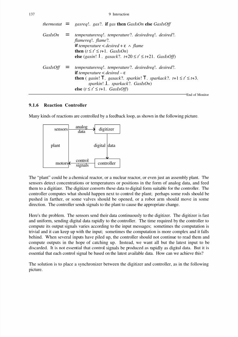
8/8/2019 37997710 Hehner a Practical Theory of Programming 2004
http://slidepdf.com/reader/full/37997710-hehner-a-practical-theory-of-programming-2004 144/242
thermostat = gasreq!. gas?. if gas then GasIsOn else GasIsOff
GasIsOn = temperaturereq!. temperature?. desiredreq!. desired ?.
flamereq!. flame?.
if temperature < desired + ε ∧ flamethen (t ≤ t ′ ≤ t +1. GasIsOn)
else (gasin! . gasack ?. t +20 ≤ t ′ ≤ t +21. GasIsOff )
GasIsOff = temperaturereq!. temperature?. desiredreq!. desired ?.
if temperature < desired – εthen ( gasin! . gasack ?. sparkin! . sparkack ?. t +1 ≤ t ′ ≤ t +3.
sparkin! . sparkack ?. GasIsOn)
else (t ≤ t ′ ≤ t +1. GasIsOff ) End of Monitor
9.1.6 Reaction Controller
Many kinds of reactions are controlled by a feedback loop, as shown in the following picture.
sensors digitizer
motors controller
plant digital data
analogdata
controlsignals
The “plant” could be a chemical reactor, or a nuclear reactor, or even just an assembly plant. Thesensors detect concentrations or temperatures or positions in the form of analog data, and feed
them to a digitizer. The digitizer converts these data to digital form suitable for the controller. The
controller computes what should happen next to control the plant; perhaps some rods should be
pushed in farther, or some valves should be opened, or a robot arm should move in some
direction. The controller sends signals to the plant to cause the appropriate change.
Here's the problem. The sensors send their data continuously to the digitizer. The digitizer is fast
and uniform, sending digital data rapidly to the controller. The time required by the controller to
compute its output signals varies according to the input messages; sometimes the computation is
trivial and it can keep up with the input; sometimes the computation is more complex and it falls
behind. When several inputs have piled up, the controller should not continue to read them andcompute outputs in the hope of catching up. Instead, we want all but the latest input to be
discarded. It is not essential that control signals be produced as rapidly as digital data. But it is
essential that each control signal be based on the latest available data. How can we achieve this?
The solution is to place a synchronizer between the digitizer and controller, as in the following
picture.
137 9 Interaction

8/8/2019 37997710 Hehner a Practical Theory of Programming 2004
http://slidepdf.com/reader/full/37997710-hehner-a-practical-theory-of-programming-2004 145/242
sensors digitizeranalogdata
controlsignals
plant synchronizer
motors controller
digital data
request reply
The synchronizer's job is as simple and uniform as the digitizer's; it can easily keep up. It
repeatedly reads the data from the digitizer, always keeping only the latest. Whenever the
controller requests some data, the synchronizer sends the latest. This is exactly the function of a
monitor, and we could implement the synchronizer that way. But a synchronizer is simpler than a
monitor in two respects: first, there is only one writing process and one reading process; second,
the writing process is uniformly faster than the reading process. Here is its definition.
synchronizer = digitaldata?.
if √request then (request ? || reply! digitaldata) else ok .synchronizer
If we were using interactive variables instead of channels, there would be no problem of reading
old data; reading an interactive variable always reads its latest value, even if the variable is written
more often than it is read. But there would be the problem of how to make sure that the interactive
variable is not read while it is being written.
End of Reaction Controller
9.1.7 Channel Declaration
The next input on a channel is not necessarily the one that was last previously written on thatchannel. In one variable x and one channel c (ignoring time),
c! 2. c?. x:= c= M w = 2 ∧ w′ = w+1 ∧ r ′ = r +1 ∧ x′ = M r
We do not know that initially w=r , so we cannot conclude that finally x′=2 . That's because
there may have been a previous write that hasn't been read yet. For example,
c! 1. c! 2. c?. x:= cThe next input on a channel is always the first one on that channel that has not yet been read. The
same is true in a parallel composition.
c! 2 || (c?. x:= c)
= M w = 2 ∧ w′ = w+1 ∧ r ′ = r +1 ∧ x′ = M r
Again we cannot say x′=2 because there may be a previous unread outputc! 1. (c! 2 || (c?. x:= c)). c?
and the final value of x may be the 1 from the earlier output, with the 2 going to the later input.
In order to achieve useful communication between processes, we have to introduce a local channel.
Channel declaration is similar to variable declaration; it defines a new channel within some local
portion of a program or specification. A channel declaration applies to what follows it, according
to the precedence table on the final page of this book. Here is a syntax and equivalent
specification.
chan c: T · P = ∃M c: [∞*T ]· ∃T c: [∞* xreal]· var r c , wc: xnat := 0· PThe type T says what communications are possible on this new channel. The declaration
9 Interaction 138

8/8/2019 37997710 Hehner a Practical Theory of Programming 2004
http://slidepdf.com/reader/full/37997710-hehner-a-practical-theory-of-programming-2004 146/242
introduces two scripts, which are infinite lists; they are not state variables, but state constants of
unknown value (mathematical variables). We have let time be extended real, but we could let it be
extended integer. The channel declaration also introduces a read cursor r c with initial value 0 to
say that initially there has been no input on this channel, and a write cursor wc with initial value 0
to say that initially there has been no output on this channel.
A local channel can be used without concurrency as a queue, or buffer. For example,
chan c: int · c! 3. c! 4. c?. x:= c. c?. x:= x+cassigns 7 to x . Here is the proof, including time.
chan c: int · c! 3. c! 4. t := max t (T r + 1). c?. x:= c. t := max t (T r + 1). c?. x:= x+c
= ∃M : [∞*int ]· ∃T : [∞* xint ]· var r , w: xnat := 0·
M w = 3 ∧ T w = t ∧ (w:= w+1).
M w = 4 ∧ T w = t ∧ (w:= w+1).
t := max t (T r + 1). r := r +1.
x:= M (r –1).
t := max t (T r + 1). r := r +1.
x:= x +M
(r –1) now use the Substitution Law several times
= ∃M : [∞*int ]· ∃T : [∞* xint ]· ∃r , r ′, w, w′: xnat ·M 0 = 3 ∧ T 0 = t ∧ M 1 = 4 ∧ T 1 = t ∧ r ′ = 2 ∧ w′ = 2 ∧ x′ = M 0 + M 1
∧ t ′ = max (max t (T 0 + 1)) (T 1 + 1) ∧ (other variables unchanged)
= x′=7 ∧ t ′ = t +1 ∧ (other variables unchanged)
Here are two processes with a communication between them. Ignoring time,
chan c: int · c! 2 || (c?. x:= c) Use the definition of local channel declaration,
and use the previous result for the independent composition
= ∃M
: [∞*int ]· var r , w: xnat := 0·M w = 2 ∧ w′ = w+1 ∧ r ′:= r +1 ∧ x′ = M r ∧ (other variables unchanged)
Now apply the initialization r := 0 and w:= 0 using the Substitution Law
= ∃M : [∞*int ]· var r , w: xnat ·M 0 = 2 ∧ w′=1 ∧ r ′=1 ∧ x′ = M 0 ∧ (other variables unchanged)
= x′=2 ∧ (other variables unchanged)
= x:= 2
Replacing 2 by an arbitrary expression, we have a general theorem equating communication on a
local channel with assignment. If we had included time, the result would have been
x′=2 ∧ t ′ = t +1 ∧ (other variables unchanged)
= x:= 2. t := t +1
End of Channel Declaration
9.1.8 Deadlock
In the previous subsection we saw that a local channel can be used as a buffer. Let's see what
happens if we try to read first and write after. Inserting the input wait into
chan c: int · c?. c! 5
gives us
139 9 Interaction
8/8/2019 37997710 Hehner a Practical Theory of Programming 2004
http://slidepdf.com/reader/full/37997710-hehner-a-practical-theory-of-programming-2004 147/242
chan c: int · t := max t (T r + 1). c?. c! 5
= ∃M : [∞*int ]· ∃T : [∞* xint ]· var r , w: xnat := 0·
t := max t (T r + 1). r := r +1. M w = 5 ∧ T w = t ∧ (w:= w+1)
We'll do this one slowly. First, expand var and w:= w+1 ,
taking r , w , x , and t as the state variables.
=∃M : [∞*int ]· ∃T : [∞* xint ]· ∃r , r ′, w, w′: xnat ·r := 0. w:= 0. t := max t (T r + 1). r := r +1.
M w = 5 ∧ T w = t ∧ r ′=r ∧ w′ = w+1 ∧ x′= x ∧ t ′=t Now use the Substitution Law four times.
= ∃M : [∞*int ]· ∃T : [∞* xint ]· ∃r , r ′, w, w′: xnat ·M 0 = 5 ∧ T 0 = max t (T 0 + 1) ∧ r ′=1 ∧ w′=1 ∧ x′= x ∧ t ′ = max t (T 0 + 1)
Look at the conjunct T 0 = max t (T 0 + 1) . For any start time t > –∞ it says T 0 = ∞ .
= x′= x ∧ t ′=∞The theory tells us that execution takes forever because the wait for input is infinite.
The word “deadlock” is usually used to mean that several processes are waiting on each other, as
in the dining philosophers example of Chapter 8. But it might also be used to mean that a singlesequential computation is waiting on itself, as in the previous paragraph. Here's the more
traditional example with two processes.
chan c, d : int · (c?. d ! 6) || (d ?. c! 7)
Inserting the input waits, we get
chan c, d : int · (t := max t (T cr c + 1). c?. d ! 6) || (t := max t (T d r d + 1). d ?. c! 7)
after a little work, we obtain
= ∃M c, M d : [∞*int ]· ∃T c, T d : [∞* xint ]· ∃r c, r c′, wc, wc′, r d , r d ′, wd , wd ′: xnat ·M d 0 = 6 ∧ T d 0 = max t (T c0 + 1) ∧ M c0 = 7 ∧ T c0 = max t (T d 0 + 1)
∧ r c′ = wc′ = r d ′ = wd ′ = 1 ∧ x′= x ∧ t ′ = max (max t (T c0 + 1)) (max t (T d 0 + 1))
Once again, for start time t >–∞ , the conjuncts
T d 0 = max t (
T c0 + 1) ∧
T c0 = max t (
T d 0 + 1) tell us that
T d 0 =
T c0 = ∞ .= x′= x ∧ t ′=∞
To prove that a computation is free from deadlock, prove that all message times are finite.
End of Deadlock
9.1.9 Broadcast
A channel consists of a message script, a time script, a read cursor, and a write cursor. Whenever
a computation splits into parallel processes, the state variables must be partitioned among the
processes. The scripts are not state variables; they do not belong to any process. The cursors are
state variables, so one of the processes can write to the channel, and one (perhaps the same one,perhaps a different one) can read from the channel. Suppose the structure is
P. (Q || R || S). T and suppose Q writes to channel c and R reads from channel c . The messages written by Q
follow those written by P , and those written by T follow those written by Q . The messages
read by R follow those read by P , and those read by T follow those read by R . There is no
problem of two processes attempting to write at the same time, and the timing discipline makes
sure that reading a message waits until after it is written.
Although communication on a channel, as defined so far, is one-way from a single writer to a
single reader, we can have as many channels as we want. So we can have two-way conversations
9 Interaction 140

8/8/2019 37997710 Hehner a Practical Theory of Programming 2004
http://slidepdf.com/reader/full/37997710-hehner-a-practical-theory-of-programming-2004 148/242
between all pairs of processes. But sometimes it is convenient to have a broadcast from one
process to more than one of the parallel processes. In the program structure of the previous
paragraph, we might want Q to write and both of R and S to read on the same channel.
Broadcast is achieved by several read cursors, one for each reading process. Then all reading
processes read the same messages, each at its own rate. There is no harm in two processes reading
the same message, even at the same time. But there is a problem with broadcast: which of the read
cursors becomes the read cursor for T ? All of the read cursors start with the same value, but they
may not end with the same value. There is no sensible way to continue reading from that channel.
So we allow broadcast on a channel only when the parallel composition is not followed
sequentially by a program that reads from that channel.
We next present a broadcast example that combines communicating processes, local channel
declaration, and dynamic process generation, in one beautiful little program. It is also a striking
example of the importance of good notation and good theory. It has been “solved” before without
them, but the “solutions” required many pages, intricate synchronization arguments, lacked proof,
and were sometimes wrong.
Exercise 415 is multiplication of power series: Write a program to read from channel a an infinitesequence of coefficients a0 a1 a2 a3 ... of a power series a0 + a1× x + a2× x2 + a3× x3 + ... and in
parallel to read from channel b an infinite sequence of coefficients b0 b1 b2 b3 ... of a power
series b0 + b1× x + b2× x2 + b3× x3 + ... and in parallel to write on channel c the infinite sequence
of coefficients c0 c1 c2 c3 ... of the power series c0 + c1× x + c2× x2 + c3× x3 + ... equal to the
product of the two input series. Assume that all inputs are already available; there are no input
delays. Produce the outputs one per time unit.
The question provides us with a notation for the coefficients: an = M a(r a+n) , bn = M b(r b+n) ,
and cn = M c(wc+n) . Let us use A , B , and C for the power series, so we can express our
desired result as
C = A× B= (a0 + a1× x + a2× x2 + a3× x3 + ... ) × (b0 + b1× x + b2× x2 + b3× x3 + ... )
= a0×b0 + (a0×b1 + a1×b0)× x + (a0×b2 + a1×b1 + a2×b0)× x2
+ (a0×b3 + a1×b2 + a2×b1 + a3×b0)× x3 + ...
from which we see cn = Σi: 0,..n+1· ai×bn–i . The question relieves us from concern with input
times, but we are still concerned with output times. The complete specification is
C = A× B ∧ ∀n· T c(wc+n) = t +n
Consider the problem: output coefficient n requires n+1 multiplications and n additions from
2×(n+1) input coefficients, and it must be produced 1 time unit after the previous coefficient. To
accomplish this requires more and more data storage, and more and more parallelism, as execution
progresses.
As usual, let us concentrate on the result first, and leave the time for later. Let
A1 = a1 + a2× x + a3× x2 + a4× x3 + ...
B1 = b1 + b2× x + b3× x2 + b4× x3 + ...
be the power series from channels a and b beginning with coefficient 1 . Then
A× B= (a0 + A1× x) × (b0 + B1× x)
= a0×b0 + (a0× B1 + A1×b0)× x + A1× B1× x2
141 9 Interaction

8/8/2019 37997710 Hehner a Practical Theory of Programming 2004
http://slidepdf.com/reader/full/37997710-hehner-a-practical-theory-of-programming-2004 149/242
In place of the problem A× B we have five new problems. The first is to read one coefficient from
each input channel and output their product; that's easy. The next two, a0× B1 and A1×b0 , are
multiplying a power series by a constant; that's easier than multiplying two power series,
requiring only a loop. The next, A1× B1 , is exactly the problem we started with, but one
coefficient farther along; it can be solved by recursion. Finally, we have to add three power series
together. Unfortunately, these three power series are not synchronized properly. We must add the
leading coefficients of a0× B
1and A
1×b
0without any coefficient from A
1× B
1, and thereafter
add coefficient n+1 of a0× B1 and A1×b0 to coefficient n of A1× B1 . To synchronize, we
move a0× B1 and A1×b0 one coefficient farther along. Let
A2 = a2 + a3× x + a4× x2 + a5× x3 + ...
B2 = b2 + b3× x + b4× x2 + b5× x3 + ...
be the power series from channels a and b beginning with coefficient 2 . Continuing the earlier
equation for A× B ,
= a0×b0 + (a0×(b1 + B2× x) + (a1 + A2× x)×b0)× x + A1× B1× x2
= a0×b0 + (a0×b1 + a1×b0)× x + (a0× B2 + A1× B1 + A2×b0)× x2
From this expansion of the desired product we can almost write a solution directly.
One problem remains. A recursive call will be used to obtain a sequence of coefficients of theproduct A1× B1 in order to produce the coefficients of A× B . But the output channel for A1× B1
cannot be channel c , the output channel for the main computation A× B . Instead, a local channel
must be used for output from A1× B1 . We need a channel parameter, for which we invent the
notation λ! . A channel parameter is really four parameters: one for the message script, one for
the time script, one for the write cursor, and one for the read cursor. (The cursors are variables, so
their parameters are reference parameters; see Chapter 5.)
Now we are ready. Define P (for product) to be our specification (ignoring time for a moment)
parameterized by output channel.
P = λ!c: rat · C = A× B
We refine P c as follows.P c ⇐ a?. b?. c! a×b.
var a0: rat := a· var b0: rat := b· chan d : rat ·P d || (a?. b?. c! a0×b + a×b0. C = a0× B + D + A×b0)
C = a0× B + D + A×b0 ⇐ a?. b?. d ?. c! a0×b + d + a×b0. C = a0× B + D + A×b0
That is the whole program: 4 lines! First, an input is read from each of channels a and b and
their product is output on channel c ; that takes care of a0×b0 . We will need these values again,
so we declare local variables (really constants) a0 and b0 to retain their values. Now that we
have read one message from each input channel, before we read another, we call P d to provide
the coefficients of A1× B1 on local channel d , in parallel with the remainder of the program.Both P d and its parallel process will be reading from channels a and b using separate read
cursors; there is no computation sequentially following them. In parallel with P d we read the
next inputs a1 and b1 and output the coefficient a0×b1 + a1×b0 . Finally we execute the loop
specified as C = a0× B + D + A×b0 , where D is the power series whose coefficients are read
from channel d .
The proof is completely straightforward. Here it is in detail.
9 Interaction 142

8/8/2019 37997710 Hehner a Practical Theory of Programming 2004
http://slidepdf.com/reader/full/37997710-hehner-a-practical-theory-of-programming-2004 150/242
a?. b?. c! a×b.
var a0: rat := a· var b0: rat := b· chan d : rat ·P d || (a?. b?. c! a0×b + a×b0. C = a0× B + D + A×b0)
= r a:= r a+1. r b:= r b+1. M cwc = M a(r a–1) × M b(r b–1) ∧ (wc:= wc+1).
∃a0, a0′, b0, b0′, M d , r d , r d ′, wd , wd ′·a0:= M
a(r
a–1). b0:= M
b(r
b–1). r
d := 0. w
d := 0.
(∀n· M d (wd +n) = (Σi: 0,..n+1· M a(r a+i) × M b(r b+n–i)))∧ (r a:= r a+1. r b:= r b+1. M cwc = a0×M b(r b–1) + M a(r a–1)×b0 ∧ (wc:= wc+1).
∀n· M c(wc+n) = a0 × M b(r b+n) + M d (r d +n) + M a(r a+n) × b0)
Make all substitutions indicated by assignments.
= M cwc = M ar a × M br b∧ ∃a0, a0′, b0, b0′, M d , r d , r d ′, wd , wd ′·
(∀n· M d n = Σi: 0,..n+1· M a(r a+1+i) × M b(r b+1+n–i))∧ M c(wc+1) = M ar a × M b(r b+1) + M a(r a+1) × M br b∧ (∀n· M c(wc+2+n) = M ar a × M b(r b+2+n) + M d n + M a(r a+2+n) × M br b)
Use the first universal quantification to replace M d n in the second.
Then throw away the first universal quantification (weakening our expression).Now all existential quantifications are unused, and can be thrown away.
⇒ M cwc = M ar a × M br b∧ M c(wc+1) = M ar a × M b(r b+1) + M a(r a+1) × M br b∧ ∀n· M c(wc+2+n) = M ar a × M b(r b+2+n)
+ (Σi: 0,..n+1· M a(r a+1+i) × M b(r b+1+n–i))+ M a(r a+2+n) × M br b
Now put the three conjuncts together.
= ∀n· M c(wc+n) = Σi: 0,..n+1· M a(r a+i) × M b(r b+n–i)= P c
We still have to prove the loop refinement.a?. b?. d ?. c! a0×b + d + a×b0. C = a0× B + D + A×b0
= r a:= r a+1. r b:= r b+1. r d := r d +1.
M cwc = a0 × M b(r b–1) + M d (r d –1) + M a(r a–1) × b0 ∧ (wc:= wc+1).
∀n· M c(wc+n) = a0 × M b(r b+n) + M d (r d +n) + M a(r a+n) × b0Make all substitutions indicated by assignments.
= M cwc = a0 × M br b + M d r d + M ar a × b0∧ ∀n· M c(wc+1+n) = a0 × M b(r b+1+n) + M d (r d +1+n) + M a(r a+1+n) × b0
Put the two conjuncts together.
= ∀n· M c(wc+n) = a0 × M b(r b+n) + M d (r d +n) + M a(r a+n) × b0
= C = a0× B + D + A×b0
According to the recursive measure of time, we must place a time increment before the recursive
call P d and before the recursive call C = a0× B + D + A×b0 . We do not need a time increment
before inputs on channels a and b according to information given in the question. We do need a
time increment before the input on channel d . Placing only these necessary time increments,
output c0 = a0×b0 will occur at time t +0 as desired, but output c1 = a0×b1 + a1×b0 will also
occur at time t +0 , which is too soon. In order to make output c1 occur at time t +1 as desired,
we must place a time increment between the first two outputs. We can consider this time increment
to account for actual computing time, or as a delay (see Chapter 5, “Time and Space Dependence”).
Here is the program with time.
143 9 Interaction

8/8/2019 37997710 Hehner a Practical Theory of Programming 2004
http://slidepdf.com/reader/full/37997710-hehner-a-practical-theory-of-programming-2004 151/242
P c ⇐ a?. b?. c! a×b.
var a0: rat := a· var b0: rat := b· chan d : rat ·(t := t +1. P d ) || (a?. b?. t := t +1. c! a0×b + a×b0. Q)
Q ⇐ a?. b?. t := max t (T d r d +1). d ?. c! a0×b + d + a×b0. t := t +1. Qwhere P is redefined, and Q is defined, as follows:
P c
= ∀n· T
c(w
c+n) = t +n
P d = ∀n· T d (wd +n) = t +nQ = (∀n· T d (r d +n) = t +n) ⇒ (∀n· T c(wc+n) = t +1+n)
We could factor the first two occurrences of t := t +1 out of the independent composition, but it
doesn't really matter. There is one change we can make to the placement of time increments that
matters greatly. Within loop Q , the assignment t := max t (T d r d +1) represents a delay of 1 time
unit the first iteration (because t = T d r d ), and a delay of 0 time units each subsequent iteration
(because t =T d r d +1 ). This makes the proof very ugly. To make the proof pretty, we can
replace t :=max t (T d r d +1) by t := max (t +1) (T d r d +1) and delete t := t +1 just before the call to
Q. These changes together do not change the timing at all; they just make the proof easier. The
assignment t := max (t +1) (T
d r d +1) increases the time by at least 1 , so the loop includes a timeincrease without the t := t +1 . The program with time is now
P c ⇐ a?. b?. c! a×b.
var a0: rat := a· var b0: rat := b· chan d : rat ·(t := t +1. P d ) || (a?. b?. t := t +1. c! a0×b + a×b0. Q)
Q ⇐ a?. b?. t := max (t +1) (T d r d +1). d ?. c! a0×b + d + a×b0. Q
In the main part of the timing proof, we accept Q as defined, without looking at its refinement.
a?. b?. c! a×b.
var a0: rat := a· var b0: rat := b· chan d : rat ·
(t := t +1. P d ) || (a?. b?. t := t +1. c! a0×b + a×b0. Q)We can ignore a? and b? because they have no effect on timing (they are substitutions for
variables that do not appear in P d and L ). We also ignore what messages are output,
looking only at their times. We can therefore also ignore variables a0 and b0 .
⇒ T cwc = t ∧ (wc:= wc+1).
∃T d , r d , r d ′, wd , wd ′· r d := 0. wd := 0.
(t := t +1. ∀n· T d (wd +n) = t +n)
∧ ( t := t +1. T cwc = t ∧ (wc:= wc+1).
(∀n· T d (r d +n) = t +n) ⇒ (∀n· T c(wc+n) = t +1+n) )
Make all substitutions indicated by assignments.
= T cwc = t
∧ ∃T d , r d , r d ′, wd , wd ′·(∀n· T d n = t +1+n)
∧ T c(wc+1) = t +1
∧ ((∀n· T d n = t +1+n) ⇒ (∀n· T c(wc+2+n) = t +2+n))
Use the first universal quantification to discharge the antecedent.
Then throw away the first universal quantification (weakening our expression).
Now all existential quantifications are unused, and can be thrown away.
⇒ T cwc = t ∧ T c(wc+1) = t +1 ∧ ∀n· T c(wc+2+n) = t +2+nNow put the three conjuncts together.
= ∀n· T c(wc+n) = t +n= P c
9 Interaction 144

8/8/2019 37997710 Hehner a Practical Theory of Programming 2004
http://slidepdf.com/reader/full/37997710-hehner-a-practical-theory-of-programming-2004 152/242
We still have to prove the loop refinement.
(Q ⇐ a?. b?. t := max (t +1) (T d r d +1). d ?. c! a0×b + d + a×b0. Q)
Ignore a? and b? and the output message.
⇐ ((∀n· T d (r d +n) = t +n) ⇒ (∀n· T c(wc+n) = t +1+n))
⇐ ( t := max (t +1) (T d r d +1). r d := r d +1. T cwc = t ∧ (wc:= wc+1).
(∀n· T d (r d +n) = t +n) ⇒ (∀n· T c(wc+n) = t +1+n) )
Use the Law of Portation to move the first antecedent
to the right side, where it becomes a conjunct.
= (∀n· T c(wc+n) = t +1+n)
⇐ (∀n· T d (r d +n) = t +n)
∧ ( t := max (t +1) (T d r d +1). r d := r d +1. T cwc = t ∧ (wc:= wc+1).
(∀n· T d (r d +n) = t +n) ⇒ (∀n· T c(wc+n) = t +1+n) )
Specializing ∀n· T d (r d +n) = t +n to the case n=0,
we use T d r d = t to simplify max (t +1) (T d r d +1).
= (∀n· T c(wc+n) = t +1+n)
⇐ (∀n· T d (r d +n) = t +n)
∧ ( t := t +1. r d := r d +1. T cwc = t ∧ (wc:= wc+1).
(∀n·T
d (r d +n) = t +n) ⇒ (∀n·T
c(wc+n) = t +1+n) )Make all substitutions indicated by assignments.
= (∀n· T c(wc+n) = t +1+n)
⇐ (∀n· T d (r d +n) = t +n)
∧ T cwc = t +1
∧ ((∀n· T d (r d +1+n) = t +1+n) ⇒ (∀n· T c(wc+1+n) = t +2+n))
The conjunct ∀n· T d (r d +n) = t +n discharges the antecedent
∀n· T d (r d +1+n) = t +1+n which can be dropped.
⇐ (∀n· T c(wc+n) = t +1+n)
⇐ T cwc = t +1 ∧ (∀n· T c(wc+1+n) = t +2+n)
= End of Broadcast
End of Communication
End of Interaction
For many students, the first understanding of programs they are taught is how programs are
executed. And for many students, that is the only understanding they are given. With that
understanding, the only method available for checking whether a program is correct is to test it by
executing it with a variety of inputs to see if the resulting outputs are right. All programs should be
tested, but there are two problems with testing.
One problem with testing is: how do you know if the outputs are right? With some programs, forexample graphics programs for producing pretty pictures, the only way to know if the output is
right is to test the program and judge the result. But other programs give answers to questions
whose answers you do not already know (that is why you wrote the program), and you cannot test
them to see if they are right. In that case, you should test to see at least if the answers are
reasonable. The other problem with testing is: you cannot try all inputs. Even if all the test cases
you try give reasonable answers, there may be problems with untried cases.
If you have read and understood this book to here, you now have an understanding of programs
that is completely different from execution. When you prove that a program refines a specification,
you are considering all inputs at once, and you are proving that the outputs have the properties
145 9 Interaction
8/8/2019 37997710 Hehner a Practical Theory of Programming 2004
http://slidepdf.com/reader/full/37997710-hehner-a-practical-theory-of-programming-2004 153/242
stated in the specification. That is far more than can ever be accomplished by testing. But it is also
more work than trying some inputs and looking at the outputs. That raises the question: when is
the extra assurance of correctness worth the extra work?
If the program you are writing is easy enough that you can probably get it right without any theory,
and it does not really matter if there are some errors in it, then the extra assurance of correctness
provided by the theory may not be worth the trouble. If you are writing a pacemaker controller for
a heart, or the software that controls a subway system, or an air traffic control program, or nuclear
power plant software, or any other programs that people's lives will depend on, then the extra
assurance is definitely worth the trouble, and you would be negligent if you did not use the theory.
To prove that a program refines a specification after the program is finished is a very difficult task.
It is much easier to perform the proof while the program is being written. The information needed
to make one step in programming is exactly the same information that is needed to prove that step
is correct. The extra work is mainly to write down that information formally. It is also the same
information that will be needed later for program modification, so writing it explicitly at each step
will save effort later. And if you find, by trying to prove a step, that the step is incorrect, you save
the effort of building the rest of your program on a wrong step. As a further bonus, after youbecome practiced and skillful at using the theory, you find that it helps in the program design; it
suggests programming steps. In the end, it may not be any extra effort at all.
In this book we have looked only at small programs, but we have done so without any automated
support. For a theory of programming to be in widespread use for industrial program design, it
must be supported by tools. Ideally, an automated prover checks each refinement, remaining silent
if the refinement is correct, complaining whenever there is a mistake, and saying exactly what is
wrong. At present there are a few tools that provide some assistance, but they are far from ideal.
There is plenty of opportunity for tool builders, and they need a thorough knowledge of a practical
theory of programming.
9 Interaction 146

8/8/2019 37997710 Hehner a Practical Theory of Programming 2004
http://slidepdf.com/reader/full/37997710-hehner-a-practical-theory-of-programming-2004 154/242
147
10 Exercises
Exercises marked with √ have been done in previous chapters.
10.0 Basic Theories
0 There are four cards on a table. On the cards you see D, E, 2, and 3 (one symbol percard). You are told that each card has a letter on one side and a digit on the other. You are
asked whether every card with a D on one side has a 3 on the other. Which card(s) do you
need to turn over to answer the question? Why? (Explain in English; no proof needed.)
1 Simplify each of the following boolean expressions.
(a) x ∧ ¬ x(b) x ∨ ¬ x(c) x ⇒ ¬ x(d) x ⇐ ¬ x(e) x = ¬ x
(f) x ¬ x
2 Prove each of the following laws of Boolean Theory using the proof format given in
Subsection 1.0.1, and any laws listed in Section 11.4. Do not use the Completion Rule.
(a) a∧b ⇒ a∨b(b) (a∧b) ∨ (b∧c) ∨ (a∧c) = (a∨b) ∧ (b∨c) ∧ (a∨c)
(c) ¬a ⇒ (a ⇒ b)
(d) a = (b ⇒ a) = a ∨ b(e) a = (a ⇒ b) = a ∧ b(f) (a⇒c) ∧ (b⇒¬c) ⇒ ¬(a∧b)
(g) a ∧ ¬b ⇒ a ∨ b
(h) (a⇒b) ∧ (c⇒d ) ∧ (a∨c) ⇒ (b∨d )(i) a ∧ ¬a ⇒ b(j) (a⇒b) ∨ (b⇒a)
(k)√ ¬(a ∧ ¬(a∨b))
(l) (¬a⇒¬b) ∧ (a b) ∨ (a∧c ⇒ b∧c)
(m) (a⇒¬a) ⇒ ¬a(n) (a⇒b) ∧ (¬a⇒b) = b(o) (a⇒b)⇒a = a(p) a=b ∨ a=c ∨ b=c(q) a∧b ∨ a∧¬b = a(r) a⇒(b⇒a)
(s) a ⇒ a ∧ b = a ⇒ b = a ∨ b ⇒ b(t) if a then a else ¬a(u) if b∧c then P else Q = if b then if c then P else Q else Q(v) if b∨c then P else Q = if b then P else if c then P else Q(w) if b then P else if b then Q else R = if b then P else R(x) if if b then c else d then P else Q
= if b then if c then P else Q else if d then P else Q(y) if b then if c then P else R else if c then Q else R
= if c then if b then P else Q else R(z) if b then if c then P else R else if d then Q else R
= if if b then c else d then if b then P else Q else R

8/8/2019 37997710 Hehner a Practical Theory of Programming 2004
http://slidepdf.com/reader/full/37997710-hehner-a-practical-theory-of-programming-2004 155/242
3 (dual) One operator is the dual of another operator if it negates the result when applied to
the negated operands. The nullary operators and are each other's duals. If
op0(¬a)= ¬(op1 a) then op0 and op1 are duals. If (¬a) op0 (¬b) = ¬(a op1 b)
then op0 and op1 are duals. And so on for more operands.
(a) Of the 4 unary boolean operators, there is 1 pair of duals, and 2 operators that are their own
duals. Find them.
(b) Of the 16 binary boolean operators, there are 6 pairs of duals, and 4 operators that are theirown duals. Find them.
(c) What is the dual of the ternary operator if then else ? Express it using only the operator
if then else .
(d) The dual of a boolean expression without variables is formed as follows: replace each
operator with its dual, adding parentheses if necessary to maintain the precedence. Explain
why the dual of a theorem is an antitheorem, and vice versa.
(e) Let P be a boolean expression without variables. From part (d) we know that every
boolean expression without variables of the form
(dual of P ) = ¬Pis a theorem. Therefore, to find the dual of a boolean expression with variables, we must
replace each operator by its dual and negate each variable. For example, if a and b areboolean variables, then the dual of a∧b is ¬a ∨ ¬b . And since
(dual of a∧b ) = ¬(a∧b)
we have one of the Duality Laws:
¬a ∨ ¬b = ¬(a ∧ b)
The other of the Duality Laws is obtained by equating the dual and negation of a∨b .
Obtain five laws that do not appear in this book by equating a dual with a negation.
(f) Dual operators have truth tables that are each other's vertical mirror reflections. For
example, the truth table for ∧ (below left) is the vertical mirror reflection of the truth table
for ∨ (below right).
∧: ∨:
Design symbols (you may redesign existing symbols where necessary) for the 4 unary and
16 binary boolean operators according to the following criteria.
(i) Dual operators should have symbols that are vertical mirror reflections (like ∧ and ∨ ).
This implies that self-dual operators have vertically symmetric symbols, and all others have
vertically asymmetric symbols.
(ii) If a op0 b = b op1 a then op0 and op1 should have symbols that are horizontal
mirror reflections (like ⇒ and ⇐ ). This implies that symmetric operators have
horizontally symmetric symbols, and all others have horizontally asymmetric symbols.
4 Truth tables and the Evaluation Rule can be replaced by a new proof rule and some new
axioms. The new proof rule says: “A boolean expression does not gain, lose, or change
classification when a theorem within it is replaced by another theorem. Similarly, a
boolean expression does not gain, lose, or change classification when an antitheorem
within it is replaced by another antitheorem.”. The truth tables become new axioms; for
example, one truth table entry becomes the axiom ∨ and another becomes the axiom
∨ . These two axioms can be reduced to one axiom by the introduction of a variable,
giving ∨ x . Write the truth tables as axioms and antiaxioms as succinctly as possible.
10 Exercises 148

8/8/2019 37997710 Hehner a Practical Theory of Programming 2004
http://slidepdf.com/reader/full/37997710-hehner-a-practical-theory-of-programming-2004 156/242
5 Complete the following laws of Boolean Theory
(a) =(b) =(c) ¬a =(d) a∧b =(e) a∨b =
(f) a=b =(g) a b =(h) a⇒b =
by adding a right side using only the following symbols (in any quantity)
(i) ¬ ∧ a b ( )
(ii) ¬ ∨ a b ( )
(iii) ¬ ⇒ a b ( )
(iv) ⇒ a b ( )
(v) ¬ if then else a b ( )
6 (BDD) A BDD (Binary Decision Diagram) is a boolean expression that has one of the
following 3 forms: , , if variable then BDD else BDD . For example,if x then if a then else else if y then if b then else else
is a BDD. An OBDD (Ordered BDD) is a BDD with an ordering on the variables, and in
each if then else , the variable in the if -part must come before any of the variables in its
then- and else-parts (“before” means according to the ordering). For example, using
alphabetic ordering for the variables, the previous example is not an OBDD, but
if a then if c then else else if b then if c then else else
is an OBDD. An LBDD (Labeled BDD) is a set of definitions of the following 3 forms:
label =
label =
label = if variable then label else label
The labels are separate from the variables; each label used in a then-part or else-part mustbe defined by one of the definitions. The following is an LBDD.
true =
false =
alice = if b then true else false
bob = if a then alice else false
An LOBDD is an LBDD that becomes an OBDD when the labels are expanded. The
ordering prevents any recursive use of the labels. The previous example is an LOBDD.
An RBDD (Reduced BDD) is a BDD such that, in each if then else , the then- and else-
parts differ. An ROBDD is both reduced and ordered; an RLBDD is both reduced and
labeled; an RLOBDD is reduced, labeled, and ordered. The previous example is an
RLOBDD.(a) Express ¬a , a∧b , a∨b , a⇒b , a=b , a b , and if a then b else c as BDDs.
(b) How can you conjoin two OBDDs and get an OBDD?
(c) How can you determine if two RLOBDDs are equal?
(d) How can we represent an RLOBDD in order to determine efficiently if an assignment of
values to variables satisfies it (solves it, gives it value )?
7 Express formally and succinctly that exactly one of three statements is true.
8 Design symbols for the 10 binary boolean operators that are not presented in Chapter 1,
and find laws about these operators.
149 10 Exercises

8/8/2019 37997710 Hehner a Practical Theory of Programming 2004
http://slidepdf.com/reader/full/37997710-hehner-a-practical-theory-of-programming-2004 157/242
9 The Case Analysis Laws equate the ternary operator if a then b else c to expressions
using only binary and unary operators. In each, the variable a appears twice. Find an
equal expression using only binary and unary operators in which the variable a appears
only once. Hint: use continuing operators.
10 Consider a fully parenthesized expression containing only the symbols = ( ) in any
quantity and any syntactically acceptable order.(a) Show that all syntactically acceptable rearrangements are equivalent.
(b) Show that it is equivalent to any expression obtained from it by making an even number of
the following substitutions: for , for , = for , for = .
11 Let p and q be boolean expressions. Suppose p is both a theorem and an antitheorem
(the theory is inconsistent).
(a) Prove, using the rules of proof presented, that q is both a theorem and an antitheorem.
(b) Is q=q a theorem or an antitheorem?
12 Formalize each of the following statements as a boolean expression. Start by staying as
close as possible to the English, then simplify as much as possible (sometimes nosimplification is possible). You will have to introduce new basic boolean expressions like
(the door can be opened) for the parts that cannot make use of boolean operators, but for
words like “only if” you should use boolean operators. You translate meanings from
words to boolean symbols; the meaning of the words may depend on their context and
even on facts not explicitly stated. Formalization is not a simple substitution of symbols
for words.
(a) The door can only be opened if the elevator is stopped.
(b) Neither the elevator door nor the floor door will open unless both of them do.
(c) Either the motor is jammed or the control is broken.
(d) Either the light is on or it is off.
(e) If you press the button, the elevator will come.(f) If the power switch is on, the system is operating.
(g) Where there's smoke, there's fire; and there's no smoke; so there's no fire.
(h) Where there's smoke, there's fire; and there's no fire; so there's no smoke.
(i) You can't score if you don't shoot.
(j) If you have a key, only then can you open the door.
(k) No pain, no gain.
(l) No shirt? No shoes? No service!
(m) If it happens, it happens.
13 Formalize each of the following statements. For each pair, either prove they are equivalent
or prove they differ.(a) Don't drink and drive.
(b) If you drink, don't drive.
(c) If you drive, don't drink.
(d) Don't drink and don't drive.
(e) Don't drink or don't drive.
14 Formalize and prove the following argument. If it is raining and Jane does not have her
umbrella with her, then she is getting wet. It is raining. Jane is not getting wet. Therefore
Jane has her umbrella with her.
10 Exercises 150
8/8/2019 37997710 Hehner a Practical Theory of Programming 2004
http://slidepdf.com/reader/full/37997710-hehner-a-practical-theory-of-programming-2004 158/242
15 A sign says: NO PARKING
7-9am
4-6pm
Mon-Fri
Using variable t for time of day and d for day, write a boolean expression that says when
there is no parking.
16 (tennis) An advertisement for a tennis magazine says “If I'm not playing tennis, I'm
watching tennis. And if I'm not watching tennis, I'm reading about tennis.”. Assuming
the speaker cannot do more than one of these activities at a time,
(a) prove that the speaker is not reading about tennis.
(b) what is the speaker doing?
17 (maid and butler) The maid said she saw the butler in the living room. The living room
adjoins the kitchen. The shot was fired in the kitchen, and could be heard in all nearby
rooms. The butler, who had good hearing, said he did not hear the shot. Given these
facts, prove that someone lied. Use the following abbreviations.
mtt = (the maid told the truth)btt = (the butler told the truth)
blr = (the butler was in the living room)
bnk = (the butler was near the kitchen)
bhs = (the butler heard the shot)
18 (knights and knaves) There are three inhabitants of an island, named P, Q, and R. Each is
either a knight or a knave. Knights always tell the truth. Knaves always lie. For each of
the following, write the given information formally, and then answer the questions, with
proof.
(a) You ask P: “Are you a knight?”. P replies: “If I am a knight, I'll eat my hat.”. Does P eat
his hat?(b) P says: “If Q is a knight, then I am a knave.”. What are P and Q?
(c) P says: “There is gold on this island if and only if I am a knight.”. Can it be determined
whether P is a knight or a knave? Can it be determined whether there is gold on the island?
(d) P, Q, and R are standing together. You ask P: “Are you a knight or a knave?”. P mumbles
his reply, and you don't hear it. So you ask Q: “What did P say?”. Q replies: “P said that
he is a knave.”. Then R says: “Don't believe Q, he's lying.”. What are Q and R?
(e) You ask P: “How many of you are knights?”. P mumbles. So Q says: “P said there is
exactly one knight among us.”. R says: “Don't believe Q, he's lying.”. What are Q and
R?
(f) P says: “We're all knaves.”. Q says: “No, exactly one of us is a knight.”. What are P, Q,
and R?
19 Islands X and Y contain knights who always tell the truth, knaves who always lie, and
possibly also some normal people who sometimes tell the truth and sometimes lie. There is
gold on at least one of the islands, and the people know which island(s) it is on. You find
a message from the pirate who buried the gold, with the following clue (which we take as
an axiom): “If there are any normal people on Island X, then there is gold on both
islands.”. You are allowed to dig on only one island, and you are allowed to ask one
question of one random person. What should you ask in order to find out which island to
dig on?
151 10 Exercises

8/8/2019 37997710 Hehner a Practical Theory of Programming 2004
http://slidepdf.com/reader/full/37997710-hehner-a-practical-theory-of-programming-2004 159/242
20 (caskets) The princess had two caskets, one gold and one silver. Into one she placed her
portrait and into the other she placed a dagger. On the gold casket she wrote the
inscription: the portrait is not in here. On the silver casket she wrote the inscription:
exactly one of these inscriptions is true. She explained to her suitor that each inscription is
either true or false (not both), but on the basis of the inscriptions he must choose a casket.
If he chooses the one with the portrait, he can marry her; if he chooses the one with the
dagger, he must kill himself. Assuming marriage is preferable to death, which casketshould he choose?
21 (the unexpected egg) There are two boxes, one red and one blue. One box has an egg in it;
the other is empty. You are to look first in the red box, then if necessary in the blue box, to
find the egg. But you will not know which box the egg is in until you open the box and
see the egg. You reason as follows: “If I look in the red box and find it empty, I'll know
that the egg is in the blue box without opening it. But I was told that I would not know
which box the egg is in until I open the box and see the egg. So it can't be in the blue box.
Now I know it must be in the red box without opening the red box. But again, that's ruled
out, so it isn't in either box.”. Having ruled out both boxes, you open them and find the
egg in one unexpectedly, as originally stated. Formalize the given statements and thereasoning, and thus explain the paradox.
22 A number can be written as a sequence of decimal digits. For the sake of generality, let us
consider using the sequence notation with arbitrary expressions, not just digits. For
example, 1(2+3)4 could be allowed, and be equal to 154 . What changes are needed to
the number axioms?
23 (scale) There is a tradition in programming languages to use a scale operator, e , in the
limited context of digit sequences. Thus 12e3 is equal to 12×103 . For the sake of
generality, let us consider using the scale notation with arbitrary expressions, not just
digits. For example, (6+6)e(5–2) could be allowed, and be equal to 12e3 . Whatchanges are needed to the number axioms?
24 When we defined number expressions, we included complex numbers such as (–1)1/2 ,
not because we particularly wanted them, but because it was easier than excluding them. If
we were interested in complex numbers, we would find that the number axioms given in
Subsection 11.4.2 do not allow us to prove many things we might like to prove. For
example, we cannot prove (–1)1/2 × 0 = 0 . How can the axioms be made strong enough
to prove things about complex numbers, but weak enough to leave room for ∞ ?
25 Express formally
(a) the absolute value of a real number x .(b) the sign of a real number x , which is –1 , 0 , or +1 depending on whether x is
negative, zero, or positive.
26 Prove –∞< y<∞ ∧ y 0 ⇒ ( x / y= z = x= z× y) .
27 Show that the number axioms become inconsistent when we add the axiom
–∞< y<∞ ⇒ x / y× y = x
28 (circular numbers) Redesign the axioms for the extended number system to make it
circular, so that +∞ = –∞ . Be careful with the transitivity of < .
10 Exercises 152
8/8/2019 37997710 Hehner a Practical Theory of Programming 2004
http://slidepdf.com/reader/full/37997710-hehner-a-practical-theory-of-programming-2004 160/242
29 Is there any harm in adding the axiom 0/0=5 to Number Theory?
30 (bracket algebra) Here is a new way to write boolean expressions. An expression can be
empty; in other words, nothing is already an expression. If you put a pair of parentheses
around an expression, you get another expression. If you put two expressions next to each
other, you get another expression. For example,
()(())((())())is an expression. The empty expression is bracket algebra's way of writing ; putting
parentheses around an expression is bracket algebra's way of negating it, and putting
expressions next to each other is bracket algebra's way of conjoining them. So the
example expression is bracket algebra's way of saying
¬ ∧¬¬ ∧¬(¬¬ ∧¬ )
We can also have variables anywhere in a bracket expression. There are three rules of
bracket algebra. If x , y , and z are any bracket expressions, then
(( x)) can replace or be replaced by x double negation rule
x() y can replace or be replaced by () base rule
x y z can replace or be replaced by x′ y z′ context rule
where x′ is x with occurrences of y added or deleted, and similarly z′ is z withoccurrences of y added or deleted. The context rule does not say how many occurrences
of y are added or deleted; it could be any number from none to all of them. To prove,
you just follow the rules until the expression disappears. For example,
((a)b((a)b)) context rule: empty for x , (a)b for y , ((a)b) for zbecomes ((a)b()) base rule: (a)b for x and empty for ybecomes (()) double negation rule
becomes
Since the last expression is empty, all the expressions are proven.
(a) Rewrite the boolean expression
¬(¬(a∧b)∧¬(¬a∧b)∧¬(a∧¬b)∧¬(¬a∧¬b))
as a bracket expression, and then prove it following the rules of bracket algebra.(b) As directly as possible, rewrite the boolean expression
(¬a⇒¬b) ∧ (a b) ∨ (a∧c ⇒ b∧c)
as a bracket expression, and then prove it following the rules of bracket algebra.
(c) Can all boolean expressions be rewritten reasonably directly as bracket expressions?
(d) Can x y become y x using the rules of bracket algebra?
(e) Can all theorems of boolean algebra, rewritten reasonably directly as bracket expressions,
be proven using the rules of bracket algebra?
(f) We interpret empty as , parentheses as negation, and juxtaposition as conjunction. Is
there any other consistent way to interpret the symbols and rules of bracket algebra?
31 Let • be a binary infix operator (precedence 3) whose operands and result are of some typeT . Let ◊ be a binary infix operator (precedence 7) whose operands are of type T and
whose result is boolean, defined by the axiom
a ◊ b = a • b = a(a) Prove if • is idempotent then ◊ is reflexive.
(b) Prove if • is associative then ◊ is transitive.
(c) Prove if • is symmetric then ◊ is antisymmetric.
(d) If T is the booleans and • is ∧ , what is ◊ ?
(e) If T is the booleans and • is ∨ , what is ◊ ?
(f) If T is the natural numbers and ◊ is ≤ , what is • ?
(g) The axiom defines ◊ in terms of • . Invert it, so that • is defined in terms of ◊ .
153 10 Exercises

8/8/2019 37997710 Hehner a Practical Theory of Programming 2004
http://slidepdf.com/reader/full/37997710-hehner-a-practical-theory-of-programming-2004 161/242
32 (family theory) Design a theory of personal relationships. Invent person expressions such
as Jack , Jill , father of p , mother of p . Invent boolean expressions that use person
expressions, such as p is male , p is female , p is a parent of q , p is a son of q , p is adaughter of q , p is a child of q , p is married to q , p=q . Invent axioms such as ( p ismale) ( p is female) . Formulate and prove an interesting theorem.
End of Basic Theories
10.1 Basic Data Structures
33 Simplify
(a) (1, 7–3) + 4 – (2, 6, 8)
(b) nat ×nat (c) nat –nat (d) (nat +1)×(nat +1)
34 Prove ¬ 7: null .
35 We defined bunch null with the axiom null: A . Is there any harm in defining bunch all with the axiom A: all ?
36 Let A be a bunch of booleans such that A = ¬ A . What is A ?
37 Show that some of the axioms of Bunch Theory listed in Section 2.0 are provable from the
other axioms. How many of the axioms can you remove without losing any theorems?
38 (hyperbunch) A hyperbunch is like a bunch except that each element can occur a number of
times other than just zero times (absent) or one time (present). The order of elements
remains insignificant. (A hyperbunch does not have a characteristic predicate, but a
characteristic function with numeric result.) Design notations and axioms for each of thefollowing kinds of hyperbunch.
(a) multibunch: an element can occur any natural number of times. For example, a multibunch
can consist of one 2, two 7s, three 5s, and zero of everything else. (Note: the equivalent
for sets is called either a multiset or a bag.)
(b) wholebunch: an element can occur any integer number of times.
(c) fuzzybunch: an element can occur any real number of times from 0 to 1 inclusive.
39 A composite number is a natural number with 2 or more (not necessarily distinct) prime
factors. Express the composite numbers as simply as you can.
40 For this question only, let # be a binary infix operator (precedence 3) with naturaloperands and an extended natural result. Informally, n#m means “the number of times
that n is a factor of m ”. It is defined by the following two axioms.
m: n×nat ∨ n#m = 0
n 0 ⇒ n# (m×n) = n#m + 1
(a) Make a 3×3 chart of the values of (0,..3)# (0,..3) .
(b) Show that the axioms become inconsistent if the antecedent of the second axiom is
removed.
(c) How should we change the axioms to allow # to have extended natural operands?
10 Exercises 154

8/8/2019 37997710 Hehner a Practical Theory of Programming 2004
http://slidepdf.com/reader/full/37997710-hehner-a-practical-theory-of-programming-2004 162/242
41 For naturals n and m , we can express the statement “ n is a factor of m ” formally as
follows:
m: n×nat (a) What are the factors of 0 ?
(b) What is 0 a factor of?
(c) What are the factors of 1 ?
(d) What is 1 a factor of?
42 Let B = 1, 3, 5 . What is
(a) ¢( B + B)
(b) ¢( B × 2)
(c) ¢( B × B)
(d) ¢( B2)
43 The compound axiom says
x: A, B = x: A ∨ x: BThere are sixteen binary boolean operators that could sit where ∨ sits in this axiom if we
just replace bunch union (,) by a corresponding bunch operator. Which of the sixteenboolean binary operators correspond to useful bunch operators?
44 (von Neumann numbers)
(a) Is there any harm in adding the axioms
0 = {null} the empty set
n+1 = {n, ~n} for each natural n(b) What correspondence is induced by these axioms between the arithmetic operations and the
set operations?
(c) Is there any harm in adding the axioms
0 = {null} the empty set
i+1 = {i, ~i} for each integer i
45 (Cantor's heaven) Show that $ 2 S > $S is neither a theorem nor an antitheorem.
46 The strings defined in Section 2.2 are “natural strings” because their lengths and indexes
are natural numbers. Invent suitable axioms for
(a) “extended strings”, including both “natural strings” and “infinite strings”.
(b) “integer strings”, including both “natural strings” and “negative strings”.
47 Prove the trichotomy for strings of numbers. For strings S and T , prove that exactly one
of S<T , S=T , S>T is a theorem.
48 In Section 2.3 there is a self-describing expression. Make it into a self-printing program.
To do so, you need to know that c!e outputs the value of expression e on channel c .
49 Simplify (no proof)
(a) null, nil(b) null; nil(c) *nil(d) [null](e) [*null]
155 10 Exercises

8/8/2019 37997710 Hehner a Practical Theory of Programming 2004
http://slidepdf.com/reader/full/37997710-hehner-a-practical-theory-of-programming-2004 163/242
50 What is the difference between [0, 1, 2] and [0; 1; 2] ?
51 (prefix order) Give axioms to define the prefix partial order on strings. String S comes
before string T in this order if and only if S is an initial segment of T .
52 Simplify, assuming i: 0,..# L
(a) i→ Li | L(b) L [0;..i] + [ x] + L [i+1;..# L]
53 Simplify (no proof)
(a) 0→1 | 1→2 | 2→3 | 3→4 | 4→5 | [0;..5]
(b) (4→2 | [–3;..3]) 3
(c) ((3;2)→[10;..15] | 3→[5;..10] | [0;..5]) 3
(d) ([0;..5] [3; 4]) 1
(e) (2;2)→`j | ["abc"; "de"; "fghi"]
(f) #[nat ](g) #[*3]
(h) [3; 4]: [3*4*int ](i) [3; 4]: [3; int ](j) [3, 4; 5]: [2*int ](k) [(3, 4); 5]: [2*int ](l) [3; (4, 5); 6; (7, 8, 9)] ‘ [3; 4; (5, 6); (7, 8)]
54 Let i and j be indexes of list L . Express i→ Lj | j→ Li | L without using | .
End of Basic Data Structures
10.2 Function Theory
55 In each of the following, replace p byλ x: int · λ y: int · λ z: int · x≥0 ∧ x2≤ y ∧ ∀ z: int· z2≤ y ⇒ z≤ x
and simplify, assuming x, y, z, u, w: int .(a) p ( x + y) (2×u + w) z(b) p ( x + y) (2×u + w)
(c) p ( x + z) ( y + y) (2+ z)
56 Some mathematicians like to use a notation like ∃! x: D· Px to mean “there is a unique x
in D such that Px holds”. Define ∃! formally.
57 Write each of the following without using § .
(a) ¢(§ x: D· Px) = 0(b) ¢(§ x: D· Px) = 1
(c) ¢(§ x: D· Px) = 2
58 (cat) Define function cat so that it applies to a list of lists and produces their catenation.
For example,
cat [[0; 1; 2]; [nil]; [[3]]; [4; 5]] = [0; 1; 2; [3]; 4; 5]
59 Express formally that L is a sublist (not necessarily consecutive items) of list M . For
example, [0; 2; 1] is a sublist of [0; 1; 2; 2; 1; 0] , but [0; 2; 1] is not a sublist of
[0;1;2;3] .
10 Exercises 156

8/8/2019 37997710 Hehner a Practical Theory of Programming 2004
http://slidepdf.com/reader/full/37997710-hehner-a-practical-theory-of-programming-2004 164/242
60 Express formally that L is a longest sorted sublist of M where
(a) the sublist must be consecutive items (a segment).
(b) the sublist must be consecutive (a segment) and nonempty.
(c) the sublist contains items in their order of appearance in M , but not necessarily
consecutively (not necessarily a segment).
61 Express formally that natural n is the length of a longest palindromic segment in list L .A palindrome is a list that equals its reverse.
62 Using the syntax x can fool y at time t formalize the statements
(a) You can fool some of the people all of the time.
(b) You can fool all of the people some of the time.
(c) You can't fool all of the people all of the time.
for each of the following interpretations of the word “You”:
(i) Someone
(ii) Anyone
(iii) The person I am talking to
63 (whodunit) Here are ten statements.
(i) Some criminal robbed the Russell mansion.
(ii) Whoever robbed the Russell mansion either had an accomplice among the servants or had
to break in.
(iii) To break in one would have to either smash the door or pick the lock.
(iv) Only an expert locksmith could pick the lock.
(v) Anyone smashing the door would have been heard.
(vi) Nobody was heard.
(vii) No one could rob the Russell mansion without fooling the guard.
(viii) To fool the guard one must be a convincing actor.
(ix) No criminal could be both an expert locksmith and a convincing actor.(x) Some criminal had an accomplice among the servants.
(a) Choosing good abbreviations, translate each of these statements into formal logic.
(b) Taking the first nine statements as axioms, prove the tenth.
64 (arity) The arity of a function is the number of variables (parameters) it introduces, and the
number of arguments it can be applied to. Write axioms to define α f (arity of f ).
65 There are some people, some keys, and some doors. Let p holds k mean that person p
holds key k . Let k unlocks d mean that key k unlocks door d . Let p opens d mean
that person p can open door d . Formalize
(a) Anyone can open any door if they have the appropriate key.(b) At least one door can be opened without a key (by anyone).
(c) The locksmith can open any door even without a key.
66 Prove that if variables i and j do not appear in predicates P and Q , then
(∀i· Pi) ⇒ (∃i· Qi) = (∃i, j· Pi ⇒ Qj)
67 There are four boolean binary associative symmetric operators with an identity. We used
two of them to define quantifiers. What happened to the other two?
68 Which binary operator can be used to define a quantifier to give the range of a function?
157 10 Exercises

8/8/2019 37997710 Hehner a Practical Theory of Programming 2004
http://slidepdf.com/reader/full/37997710-hehner-a-practical-theory-of-programming-2004 165/242
69 We have defined several quantifiers by starting with an associative symmetric operator with
an identity. Bunch union is also such an operator. Does it yield a quantifier?
70 Exercise 13 talks about drinking and driving, but not about time. It's not all right to drink
first and then drive soon after, but it is all right to drive first and then drink soon after. It is
also all right to drink first and then drive 6 hours after. Let drink and drive be predicates
of time, and formalize the rule that you can't drive for 6 hours after drinking. What doesyour rule say about drinking and driving at the same time?
71 Formalize each of the following statements as a boolean expression.
(a) Everybody loves somebody sometime.
(b) Every 10 minutes someone in New York City gets mugged.
(c) Every 10 minutes someone keeps trying to reach you.
(d) Whenever the altititude is below 1000 feet, the landing gear must be down.
(e) I'll see you on Tuesday, if not before.
(f) No news is good news.
72 Express formally that(a) natural n is the largest proper (neither 1 nor m ) factor of natural m .
(b) g is the greatest common divisor of naturals a and b .
(c) m is the lowest common multiple of naturals a and b .
(d) p is a prime number.
(e) n and m are relatively prime numbers.
(f) there is at least one and at most a finite number of naturals satisfying predicate p .
(g) there is no smallest integer.
(h) between every two rational numbers there is another rational number.
(i) list L is a longest segment of list M that does not contain item x .
(j) the segment of list L from (including) index i to (excluding) index j is a segment whose
sum is smallest.(k) a and b are items of lists A and B (respectively) whose absolute difference is least.
(l) p is the length of a longest plateau (segment of equal items) in a nonempty sorted list L .
(m) all items that occur in list L occur in a segment of length 10 .
(n) all items of list L are different (no two items are equal).
(o) at most one item in list L occurs more than once.
(p) the maximum item in list L occurs m times.
(q) list L is a permutation of list M .
73 (bitonic list) A list is bitonic if it is monotonic up to some index, and antimonotonic after
that. For example, [1; 3; 4; 5; 5; 6; 4; 4; 3] is bitonic. Express formally that L is bitonic.
74 Formalize and disprove the statement “There is a natural number that is not equal to any
natural number.”.
75 (friends) Formalize and prove the statement “The people you know are those known by all
who know all whom you know.”.
76 (swapping partners) There is a finite bunch of couples. Each couple consists of a man and
a woman. The oldest man and the oldest woman have the same age. If any two couples
swap partners, forming two new couples, the younger partners of the two new couples
have the same age. Prove that in each couple, the partners have the same age.
10 Exercises 158

8/8/2019 37997710 Hehner a Practical Theory of Programming 2004
http://slidepdf.com/reader/full/37997710-hehner-a-practical-theory-of-programming-2004 166/242
8/8/2019 37997710 Hehner a Practical Theory of Programming 2004
http://slidepdf.com/reader/full/37997710-hehner-a-practical-theory-of-programming-2004 167/242
89 If f : A→ B and p: B→bool , prove
(a) ∃b: fA· pb = ∃a: A· pfa(b) ∀b: fA· pb = ∀a: A· pfa
90 This question explores a simpler, more elegant function theory than the one presented in
Chapter 3. We separate the notion of local variable introduction from the notion of domain,
and we generalize the latter to become local axiom introduction. Variable introduction hasthe form λv· b where v is a variable and b is any expression (the body; no domain).
There is a Renaming Axiom
λv· b = λw· (substitute w for v in b )
and an Application Axiom
(λv· b) x = (substitute x for v in b )
Let a be boolean, and let b be any expression. Then a b is an expression of the same
type as b . The operator has precedence level 12 and is right-associating. Its axioms
include:
b = ba b c = a∧b c
The expression a b is a “one-tailed if-expression”, or “asserted expression”; itintroduces a as a local axiom within b . A function is a variable introduction whose body
is an asserted expression in which the assertion has the form v: D . In this case, we allow
an abbreviation: for example, the function λ n · n : nat n+1 can be abbreviated
λn:nat ·n+1 . Applying this function to 3 , we find
(λn· n: nat n+1) 3
= 3: nat 3+1
= 4
= 4
Applying it to –3 we find
(λn· n: nat n+1) (–3)
= –3: nat –3+1= –2
and then we are stuck; no further axiom applies. In the example, we have used variable
introduction and axiom introduction together to give us back the kind of function we had;
but in general, they are independently useful.
(a) Show how function-valued variables can be introduced in this new theory.
(b) What expressions in the old theory have no equivalent in the new? How closely can they
be approximated?
(c) What expressions in the new theory have no equivalent in the old? How closely can they
be approximated?
91 Is there any harm in defining relation R with the following axioms?∀ x· ∃ y· Rxy totality
∀ x· ¬ Rxx irreflexivity
∀ x, y, z· Rxy ∧ Ryz ⇒ Rxz transitivity
∃u· ∀ x· x=u ∨ Rxu unity
92 Let n be a natural number, and let R be a relation on 0,..n . In other words,
R: (0,..n) → (0,..n) → boolWe say that from x we can reach x in zero steps. If Rxy we say that from x we can
reach y in one step. If Rxy and Ryz we say that from x we can reach z in two steps.
And so on. Express formally that from x we can reach y in some number of steps.
10 Exercises 160
8/8/2019 37997710 Hehner a Practical Theory of Programming 2004
http://slidepdf.com/reader/full/37997710-hehner-a-practical-theory-of-programming-2004 168/242
93 Relation R is transitive if ∀ x, y, z· Rxy ∧ Ryz ⇒ Rxz . Express formally that relation R
is the transitive closure of relation Q ( R is the strongest transitive relation that is implied
by Q ).
End of Function Theory
10.3 Program Theory
94 Prove specification S is satisfiable for prestate σ if and only if S. (note: is the
“true” boolean).
95 Let x be an integer state variable. Which of the following specifications are
implementable?
(a) x ≥ 0 ⇒ x′ 2 = x(b) x′ ≥ 0 ⇒ x = 0
(c) ¬( x ≥ 0 ∧ x′ = 0)
(d) ¬( x ≥ 0 ∨ x′ = 0)
96 A specification is transitive if, for all states a , b , and c , if it allows the state to changefrom a to b , and it allows the state to change from b to c , then it allows the state to
change from a to c . Prove S is transitive if and only if S is refined by S.S .
97√ Simplify each of the following (in integer variables x and y ).
(a) x:= y+1. y′> x′(b) x:= x+1. y′> x ∧ x′> x(c) x:= y+1. y′=2 x(d) x:= 1. x≥1 ⇒ ∃ x· y′=2 x(e) x:= y. x≥1 ⇒ ∃ y· y′= x× y(f) x:= 1. ok
(g) x:= 1. y:= 2(h) x:= 1. P where P = y:= 2
(i) x:= 1. y:= 2. x:= x+ y(j) x:= 1. if y> x then x:= x+1 else x:= y(k) x:= 1. x′> x. x′= x+1
98 Prove
(a) x:= x = ok (b) x:= e. x:= f x = x:= f e
99 Prove or disprove
(a) R. if b then P else Q = if b then ( R. P) else ( R. Q)(b) if b then P⇒Q else R⇒S = (if b then P else R) ⇒ (if b then Q else S)
(c) if b then (P. Q) else ( R. S) = if b then P else R. if b then Q else S
100 Prove
(a) P and Q are each refined by R if and only if their conjunction is refined by R .
(b) P⇒Q is refined by R if and only if Q is refined by P∧ R .
101 (roll up) Suppose S ⇐ A. A. S. Z . Z . Can we conclude S ⇐ A. S. Z ? Can we
always roll up a loop?
161 10 Exercises
8/8/2019 37997710 Hehner a Practical Theory of Programming 2004
http://slidepdf.com/reader/full/37997710-hehner-a-practical-theory-of-programming-2004 169/242
102 What is wrong with the following proof:
( R ⇐ R. S) use context rule
= ( R ⇐ . S) is base for .
= ( R ⇐ ) base law for ⇐=
103 For which kinds of specifications P and Q is the following a theorem:(a) ¬(P. ¬Q) ⇐ P. Q(b) P. Q ⇐ ¬(P. ¬Q)
(c) P. Q = ¬(P. ¬Q)
104 Write a formal specification of the following problem: “Change the value of list variable L
so that each item is repeated. For example, if L is [6; 3; 5; 5; 7] then it should be
changed to [6; 6; 3; 3; 5; 5; 5; 5; 7; 7] .”.
105 Let P and Q be specifications. Let C be a precondition and let C ′ be the corresponding
postcondition. Prove the condition law
P. Q ⇐ P∧C ′. C ⇒Q
106 Let P and Q be specifications. Let C be a precondition and let C ′ be the corresponding
postcondition. Which three of the following condition laws can be turned around,
switching the problem and the solution?
C ∧ (P. Q) ⇐ C ∧P. QC ⇒ (P.Q) ⇐ C ⇒P. Q(P.Q) ∧ C ′ ⇐ P. Q∧C ′(P.Q) ⇐ C ′ ⇐ P. Q⇐C ′P. C ∧Q ⇐ P∧C ′. QP. Q ⇐ P∧C ′. C ⇒Q
107 Let S be a specification. Let C be a precondition and let C ′ be the corresponding
postcondition. How does the exact precondition for C ′ to be refined by S differ from
(S.C ) ? Hint: consider prestates in which S is unsatisfiable, then deterministic, then
nondeterministic.
108 We have Refinement by Steps, Refinement by Parts, and Refinement by Cases. In this
question we propose Refinement by Alternatives:
If A ⇐ if b then C else D and E ⇐ if b then F else G are theorems,
then A∨ E ⇐ if b then C ∨F else D∨G is a theorem.
If A ⇐ B.C and D ⇐ E .F are theorems, then A∨ D ⇐ B∨ E . C ∨F is a theorem.
If A ⇐ B and C ⇐ D are theorems, then A∨C ⇐ B∨ D is a theorem.Discuss the merits and demerits of this proposed law.
109 Let x and y be real variables. Prove that if y= x2 is true before
x:= x+1. y:= y + 2× x – 1
then it is still true after.
110√ In one integer variable x ,
(a) find the exact precondition A for x′>5 to be refined by x:= x+1 .
(b) find the exact postcondition for A to be refined by x:= x+1 , where A is your answer
from part (a).
10 Exercises 162

8/8/2019 37997710 Hehner a Practical Theory of Programming 2004
http://slidepdf.com/reader/full/37997710-hehner-a-practical-theory-of-programming-2004 170/242
111 Let all variables be natural except L is a list of naturals. What is the exact precondition for
(a) x′+ y′ > 8 to be refined by x:= 1
(b) x′=1 to be refined by x:= 1
(c) x′=2 to be refined by x:= 1
(d) x′= y to be refined by y:= 1
(e) x′ ≥ y′ to be refined by x:= y+ z
(f) y′+ z′ ≥ 0 to be refined by x:= y+ z(g) x′≤1 ∨ x′≥5 to be refined by x:= x+1
(h) x′< y′ ∧ ∃ x· Lx< y′ to be refined by x:= 1
(i) ∃ y· Ly< x′ to be refined by x:= y+1
(j) L′ 3 = 4 to be refined by L:= i→4 | L(k) x′=a to be refined by if a > b then x:= a else ok (l) x′= y ∧ y′= x to be refined by ( z:= x. x:= y. y:= z)
(m) a× x′ 2 + b× x′ + c = 0 to be refined by ( x:= a× x + b. x:= – x / a)
(n) f ′ = n′! to be refined by (n:= n+1. f := f ×n) where ! means factorial.
(o) 7 ≤ c′ < 28 ∧ odd c′ to be refined by (a:= b–1. b:= a+3. c:= a+b)
(p) s′ = Σ L [0;..i′] to be refined by (s:= s + Li. i:= i+1)
112 For what exact precondition and postcondition does the following assignment move integer
variable x farther from zero?
(a) x:= x+1
(b) x:= abs ( x+1)
(c)√ x:= x2
113 For what exact precondition and postcondition does the following assignment move integer
variable x farther from zero staying on the same side of zero?
(a) x:= x+1
(b) x:= abs ( x+1)
(c) x:= x2
114 Prove
(a) the Precondition Law: C is a sufficient precondition for P to be refined by S if and only
if C ⇒P is refined by S .
(b) the Postcondition Law: C ′ is a sufficient postcondition for P to be refined by S if and
only if C ′⇒P is refined by S .
115 (weakest prespecification, weakest postspecification) Given specifications P and Q , find
the weakest specification S (in terms of P and Q ) such that P is refined by
(a) S. Q
(b) Q. S
116 Let a , b , and c be integer variables. Simplify
(a) b:= a–b. b:= a–b(b) a:= a+b. b:= a–b. a:= a–b(c) c:= a–b–c. b:= a–b–c. a:= a–b–c. c:= a+b+c
117 Let x and y be boolean variables. Simplify
(a) x:= x= y. x:= x= y(b) x:= x y. y:= x y. x:= x y
163 10 Exercises

8/8/2019 37997710 Hehner a Practical Theory of Programming 2004
http://slidepdf.com/reader/full/37997710-hehner-a-practical-theory-of-programming-2004 171/242
118 Let x be an integer variable. Prove the refinement
(a)√ x′=0 ⇐ if x=0 then ok else ( x:= x–1. x′=0)
(b) P ⇐ if x=0 then ok else ( x:= x–1. t := t +1. P)
where P = x′=0 ∧ if x≥0 then t ′ = t + x else t ′=∞
119 Let x be an integer variable. Prove the refinement
(a) x′=1 ⇐ if x=1 then ok else ( x:= div x 2. x′=1)(b)√ R ⇐ if x=1 then ok else ( x:= div x 2. t := t +1. R)
where R = x′=1 ∧ if x≥1 then t ′ ≤ t + log x else t ′=∞
120 In natural variables s and n prove
P ⇐ if n=0 then ok else (n:= n–1. s:= s+2n–n. t := t +1. P)
where P = s′ = s + 2n – n×(n–1)/2 – 1 ∧ n′=0 ∧ t ′ = t +n .
121 Is the refinement
P ⇐ if x=0 then ok else ( x:= x–1. t := t +1. P)
a theorem when
P = x<0 ⇒ x′=1 ∧ t ′=∞Is this reasonable? Explain.
122 (factorial) In natural variables n and f prove
f := n! ⇐ if n=0 then f := 1 else (n:= n–1. f := n!. n:= n+1. f := f ×n)
where n! = 1×2×3×...×n .
123 In natural variables n and m prove
P ⇐ n:= n+1.
if n=10 then ok else (m:= m–1. P)
where P = m:= m+n–9. n:= 10 .
124 Let x and n be natural variables. Find a specification P such that both the following
hold:
x = x′×2n′ ⇐ n:= 0. PP ⇐ if even x then ( x:= x /2. n:= n+1. P) else ok
125 (square) Let s and n be natural variables. Find a specification P such that both the
following hold:
s′ = n2 ⇐ s:= n. PP ⇐ if n=0 then ok else (n:= n–1. s:= s+n+n. P)
This program squares using only addition, subtraction, and test for zero.
126 Let a and b be positive integers. Let x , u , and v be integer variables. Let
P = u≥0 ∧ v≥0 ∧ x = u×a – v×b ⇒ x′=0
(a) Prove
P ⇐ if x>0 then ( x:= x–a. u:= u–1. P)
else if x<0 then ( x:= x+b. v:= v–1. P)
else ok (b) Find an upper bound for the execution time of the program in part (a).
10 Exercises 164

8/8/2019 37997710 Hehner a Practical Theory of Programming 2004
http://slidepdf.com/reader/full/37997710-hehner-a-practical-theory-of-programming-2004 172/242
127 Let i be an integer variable. Add time according to the recursive measure, and then find
the strongest P you can such that
(a) P ⇐ if even i then i:= i /2 else i:= i+1.
if i=1 then ok else P(b) P ⇐ if even i then i:= i /2 else i:= i–3.
if i=0 then ok else P
128 Find a finite function f of natural variables i and j to serve as an upper bound on the
execution time of the following program, and prove
t ′ ≤ t + fij ⇐ if i=0 ∧ j=0 then ok else if i=0 then (i:= j× j. j:= j–1. t := t +1. t ′ ≤ t + fij)else (i:= i–1. t := t +1. t ′ ≤ t + fij)
129 Let P mean that the final values of natural variables a and b are the largest exponents of
2 and 3 respectively such that both powers divide evenly into the initial value of positive
integer x .
(a) Define P formally.
(b) Define Q suitably and proveP ⇐ a:= 0. b:= 0. QQ ⇐ if x: 2×nat then ( x:= x /2. a:= a+1. Q)
else if x: 3×nat then ( x:= x /3. b:= b+1. Q)
else ok (c) Find an upper bound for the execution time of the program in part (b).
130 Express formally that specification R is satisfied by any number (including 0 ) of
repetitions of behavior satisfying specification S .
131 (Zeno) Here is a loop.
R ⇐ x:= x+1. RSuppose we charge time 2– x for the recursive call, so that each iteration takes half as long
as the one before. Prove that the execution time is finite.
132 Can we prove the refinement
P ⇐ t := t +1. Pfor P = t ′=5 ? Does this mean that execution will terminate at time 5 ? What is wrong?
133 Let n and r be natural variables in the refinement
P ⇐ if n=1 then r := 0 else (n:= div n 2. P. r := r +1)
Suppose the operations div and + each take time 1 and all else is free (even the call is
free). Insert appropriate time increments, and find an appropriate P to express theexecution time in terms of
(a) the initial values of the memory variables. Prove the refinement for your choice of P .
(b) the final values of the memory variables. Prove the refinement for your choice of P .
134 (running total) Given list variable L and any other variables you need, write a program to
convert L into a list of cumulative sums. Formally,
(a) ∀n: 0,..# L· L′n = Σ L [0;..n]
(b) ∀n: 0,..# L· L′n = Σ L [0;..n+1]
135 (cube) Write a program that cubes using only addition, subtraction, and test for zero.
165 10 Exercises

8/8/2019 37997710 Hehner a Practical Theory of Programming 2004
http://slidepdf.com/reader/full/37997710-hehner-a-practical-theory-of-programming-2004 173/242
136 (cube test) Write a program to determine if a given natural number is a cube without using
exponentiation.
137 ( mod 2 ) Let n be a natural variable. The problem to reduce n modulo 2 can be solved
as follows:
n′ = mod n 2 ⇐ if n<2 then ok else (n:= n–2. n′ = mod n 2)
Using the recursive time measure, find and prove an upper time bound. Make it as small asyou can.
138 (fast mod 2 ) Let n and p be natural variables. The problem to reduce n modulo 2 can
be solved as follows:
n′ = mod n 2 ⇐ if n<2 then ok else (even n′ = even n. n′ = mod n 2)
even n′ = even n ⇐ p:= 2. even p ⇒ even p′ ∧ even n′ = even neven p ⇒ even p′ ∧ even n′ = even n ⇐
n:= n– p. p:= p+ p.
if n< p then ok else even p ⇒ even p′ ∧ even n′ = even n(a) Prove these refinements.
(b) Using the recursive time measure, find and prove a sublinear upper time bound.
139 Given a specification P and a prestate σ with t as time variable, we might define “the
exact precondition for termination” as follows:
∃n: nat · ∀σ′· t ′ ≤ t +n ⇐ PLetting x be an integer variable, find the exact precondition for termination of the
following, and comment on whether it is reasonable.
(a) x ≥ 0 ⇒ t ′ ≤ t + x(b) ∃n: nat · t ′ ≤ t +n(c) ∃ f : int →nat · t ′ ≤ t + fx
140√ (maximum item) Write a program to find the maximum item in a list.
141 (list comparison) Using item comparison but not list comparison, write a program to
determine whether one list comes before another in the list order.
142√ (list summation) Write a program to find the sum of a list of numbers.
143 (alternating sum) Write a program to find the alternating sum L0 – L1 + L2 – L3 + L4 –
... of a list L of numbers.
144 (combinations) Write a program to find the number of ways to partition a+b things into a
things and b things. Include recursive time.
145 (earliest meeting time) Write a program to find the earliest meeting time acceptable to three
people. Each person is willing to state their possible meeting times by means of a function
that tells, for each time t , the earliest time at or after t that they are available for a meeting.
(Do not confuse this t with the execution time variable. You may ignore execution time
for this problem.)
146 (polynomial) You are given n: nat , c: [n*rat ] , x: rat and variable y: rat . c is a list of
coefficients of a polynomial (“of degree n–1”) to be evaluated at x . Write a program for
y′ = Σi: 0,..n· ci× xi
10 Exercises 166
8/8/2019 37997710 Hehner a Practical Theory of Programming 2004
http://slidepdf.com/reader/full/37997710-hehner-a-practical-theory-of-programming-2004 174/242
147 (multiplication table) Given n: nat and variable M : [*[*nat ]] , write a program to assign
to M a multiplication table of size n without using multiplication. For example, if
n =4, then
M ′ = [ [0];
[0; 1];
[0; 2; 4];
[0; 3; 6; 9] ]
148 (Pascal's triangle) Given n: nat and variable P: [*[*nat ]] , write a program to assign to P
a Pascal's triangle of size n . For example, if n = 4 , then
P′ = [ [1];
[1; 1];
[1; 2; 1];
[1; 3; 3; 1] ]
The left side and diagonal are all 1s; each interior item is the sum of the item above it and
the item diagonally above and left.
149√ (binary exponentiation) Given natural variables x and y , write a program for y′ = 2 x without using exponentiation.
150 Write a program to find the smallest power of 2 that is bigger than or equal to a given
positive integer without using exponentiation.
151√ (fast exponentiation) Given rational variables x and z and natural variable y , write a
program for z′ = x y that runs fast without using exponentiation.
152 (sort test) Write a program to assign a boolean variable to indicate whether a given list is
sorted.
153√ (linear search) Write a program to find the first occurrence of a given item in a given list.
The execution time must be linear in the length of the list.
154√ (binary search) Write a program to find a given item in a given nonempty sorted list. The
execution time must be logarithmic in the length of the list. The strategy is to identify
which half of the list contains the item if it occurs at all, then which quarter, then which
eighth, and so on.
155 (binary search with test for equality) The problem is binary search (Exercise 154), but each
iteration tests to see if the item in the middle of the remaining segment is the item we seek.
(a) Write the program, with specifications and proofs.(b) Find the execution time according to the recursive measure.
(c) Find the execution time according to a measure that charges time 1 for each test.
(d) Compare the execution time to binary search without the test for equality each iteration.
156 (ternary search) The problem is the same as binary search (Exercise 154). The strategy
this time is to identify which third of the list contains the item if it occurs at all, then which
ninth, then which twenty-seventh, and so on.
157√ (two-dimensional search) Write a program to find a given item in a given 2-dimensional
array. The execution time must be linear in the product of the dimensions.
167 10 Exercises
8/8/2019 37997710 Hehner a Practical Theory of Programming 2004
http://slidepdf.com/reader/full/37997710-hehner-a-practical-theory-of-programming-2004 175/242
158 (sorted two-dimensional search) Write a program to find a given item in a given 2-
dimensional array in which each row is sorted and each column is sorted. The execution
time must be linear in the sum of the dimensions.
159 (sorted two-dimensional count) Write a program to count the number of occurrences of a
given item in a given 2-dimensional array in which each row is sorted and each column is
sorted. The execution time must be linear in the sum of the dimensions.
160 (pattern search) Let subject and pattern be two texts. Write a program to do the
following. If pattern occurs somewhere within subject , natural variable h is assigned to
indicate the beginning of its first occurrence
(a) using any list operators given in Section 2.3.
(b) using list indexing, but no other list operators.
161 (fixed point) Let L be a nonempty sorted list of n different integers. Write a program to
find a fixed-point of L , that is an index i such that Li = i , or to report that no such index
exists. Execution time should be at most log n where n is the length of the list.
162 (all present) Given a natural number and a list, write a program to determine if every
natural number up to the given number is an item in the list.
163 (missing number) You are given a list of length n whose items are the numbers 0,..n+1
in some order, but with one number missing. Write a program to find the missing number.
164 (text length) You are given a text (list of characters) that begins with zero or more
“ordinary” characters, and then ends with zero or more “padding” characters. A padding
character is not an ordinary character. Write a program to find the number of ordinary
characters in the text. Execution time should be logarithmic in the text length.
165 (ordered pair search) Given a list of at least two items whose first item is less than or equal
to its last item, write a program to find an adjacent pair of items such that the first of the
pair is less than or equal to the second of the pair. Execution time should be logarithmic in
the length of the list.
166 (convex equal pair) A list of numbers is convex if its length is at least 2 , and every item
(except the first and last) is less than or equal to the average of its two neighbors. Given a
convex list, write a program to determine if it has a pair of consecutive equal items.
Execution should be logarithmic in the length of the list.
167 Define a partial order « on pairs of integers as follows:[a; b] « [c; d ] = a<c ∧ b<d
Given n: nat +1 and L: [n*[int ; int ]] write a program to find the index of a minimal item in
L . That is, find j: 0,..# L such that ¬∃i· Li « Lj . The execution time should be at most
n×log n .
168 ( n sort) Given a list L such that L (0,..# L) = 0,..# L , write a program to sort L in
linear time and constant space. The only change permitted to L is to swap two items.
169√ ( n2 sort) Write a program to sort a list. Execution time should be at most n2 where n is
the length of the list.
10 Exercises 168

8/8/2019 37997710 Hehner a Practical Theory of Programming 2004
http://slidepdf.com/reader/full/37997710-hehner-a-practical-theory-of-programming-2004 176/242
170 ( n × log n sort) Write a program to sort a list. Execution time should be at most n × log n
where n is the length of the list.
171 (reverse) Write a program to reverse the order of the items of a list.
172 (next sorted list) Given a sorted list of naturals, write a program to find the next (in list
order) sorted list having the same sum.
173 (next combination) You are given a sorted list of m different numbers, all in the range
0,..n . Write a program to find the lexicographically next sorted list of m different
numbers, all in the range 0,..n .
174 (next permutation) You are given a list of the numbers 0,..n in some order. Write a
program to find the lexicographically next list of the numbers 0,..n .
175 (permutation inverse) You are given a list variable P of different items in 0,..#P . Write
a program for P P′ = [0;..#P] .
176 (idempotent permutation) You are given a list variable L of items in 0,..# L (not
necessarily all different). Write a program to permute the list so that finally L′ L′ = L′ .
177 (local minimum) You are given a list L of at least 3 numbers such that L0 ≥ L1 and
L(# L–2) ≤ L(# L–1) . A local minimum is an interior index i: 1,..# L–1 such that
L(i–1) ≥ Li ≤ L(i+1)
Write a program to find a local minimum of L .
178 (natural division) The natural quotient of natural n and positive integer p is the natural
number q satisfying
q ≤ n / p < q+1Write a program to find the natural quotient of n and p in log n time without using any
functions ( div , mod , floor , ceil , ... ).
179 (remainder) Write a program to find the remainder after natural division (Exercise 178),
using only comparison, addition, and subtraction (not multiplication or division or mod ).
180 (natural binary logarithm) The natural binary logarithm of a positive integer p is the
natural number b satisfying
2b ≤ p < 2b+1
Write a program to find the natural binary logarithm of a given positive integer p in log p
time.
181 (natural square root) The natural square root of a natural number n is the natural number
s satisfying
s2 ≤ n < (s+1)2
(a) Write a program to find the natural square root of a given natural number n in log n time.
(b) Write a program to find the natural square root of a given natural number n in log n time
using only addition, subtraction, doubling, halving, and comparisons (no multiplication or
division).
169 10 Exercises

8/8/2019 37997710 Hehner a Practical Theory of Programming 2004
http://slidepdf.com/reader/full/37997710-hehner-a-practical-theory-of-programming-2004 177/242
182 (factor count) Write a program to find the number of factors (not necessarily prime) of a
given natural number.
183 (Fermat's last program) Given natural c , write a program to find the number of unordered
pairs of naturals a and b such that a2 + b2 = c2 in time proportional to c . (An
unordered pair is really a bunch of size 1 or 2 . If we have counted the pair a and b ,
we don't want to count the pair b and a .) Your program may use addition, subtraction,multiplication, division, and comparisons, but not exponentiation or square root.
184 (flatten) Write a program to flatten a list. The result is a new list just like the old one but
without the internal structure. For example,
L = [ [3; 5]; 2; [5; [7]; [nil] ] ] L′ = [3; 5; 2; 5; 7]
Your program may employ a test Li: int to see if an item is an integer or a list.
185 (diagonal) Some points are arranged around the perimeter of a circle. The distance from
each point to the next point going clockwise around the perimeter is given by a list. Write a
program to find two points that are farthest apart.
186 (minimum sum segment) Given a list of integers, possibly including negatives, write a
program to find
(a)√ the minimum sum of any segment (sublist of consecutive items).
(b) the segment (sublist of consecutive items) whose sum is minimum.
187 (maximum product segment) Given a list of integers, possibly including negatives, write a
program to find
(a) the maximum product of any segment (sublist of consecutive items).
(b) the segment (sublist of consecutive items) whose product is maximum.
188 (segment sum count)
(a) Write a program to find, in a given list of naturals, the number of segments whose sum is a
given natural.
(b) Write a program to find, in a given list of positive naturals, the number of segments whose
sum is a given natural.
189 (longest plateau) You are given a nonempty sorted list of numbers. A plateau is a segment
(sublist of consecutive items) of equal items. Write a program to find
(a) the length of a longest plateau.
(b) the number of longest plateaus.
190 (longest smooth segment) In a list of integers, a smooth segment is a sublist of consecutive
items in which no two adjacent items differ by more than 1 . Write a program to find a
longest smooth segment.
191 (longest balanced segment) Given a list of booleans, write a program to find a longest
segment (sublist of consecutive items) having an equal number of and items.
192 (longest palindrome) A palindrome is a list that equals its reverse. Write a program to find
a longest palindromic segment in a given list.
10 Exercises 170

8/8/2019 37997710 Hehner a Practical Theory of Programming 2004
http://slidepdf.com/reader/full/37997710-hehner-a-practical-theory-of-programming-2004 178/242
193 (greatest subsequence) Given a list, write a program to find the sublist that is largest
according to list order. (A sublist contains items drawn from the list, in the same order of
appearance, but not necessarily consecutive items.)
194 Given a list whose items are all 0 , 1 , or 2 , write a program
(a) to find the length of a shortest segment (consecutive items) that contains all three numbers
in any order.(b) to count the number of sublists (not necessarily consecutive items) that are 0 then 1 then
2 in that order.
195 Let L and M be sorted lists of numbers. Write a program to find the number of pairs of
indexes i: 0,..# L and j: 0,..# M such that Li ≤ Mj .
196 (heads and tails) Let L be a list of positive integers. Write a program to find the number
of pairs of indexes i and j such that
Σ L [0;..i] = Σ L [ j;..# L]
197 (pivot) You are given a nonempty list of positive numbers. Write a program to find thebalance point, or pivot. Each item contributes its value (weight) times its distance from the
pivot to its side of the balance. Item i is considered to be located at point i + 1/2 , and the
pivot point may likewise be noninteger.
198 (inversion count) Given a list, write a program to find how many pairs of items (not
necessarily consecutive items) are out of order, with the larger item before the smaller item.
199 (minimum difference) Given two nonempty sorted lists of numbers, write a program to
find a pair of items, one from each list, whose absolute difference is smallest.
200 (earliest quitter) In a nonempty list find the first item that is not repeated later. In list[13;14; 15; 14; 15; 13] the earliest quitter is 14 because the other items 13 and 15 both
occur after the last occurrence of 14 .
201 (interval union) A collection of intervals along a real number line is given by the list of left
ends L and the corresponding list of right ends R . List L is sorted. The intervals might
sometimes overlap, and sometimes leave gaps. Write a program to find the total length of
the number line that is covered by these intervals.
202 (bit sum) Write a program to find the number of ones in the binary representation of a
given natural number.
203 (digit sum) Write a program to find the sum of the digits in the decimal representation of a
given natural number.
204 (parity check) Write a program to find whether the number of ones in the binary
representation of a given natural number is even or odd.
205 (approximate search) Given a nonempty sorted list of numbers and a number, write a
program to determine the index of an item in the list that is closest in value to the given
number.
171 10 Exercises

8/8/2019 37997710 Hehner a Practical Theory of Programming 2004
http://slidepdf.com/reader/full/37997710-hehner-a-practical-theory-of-programming-2004 179/242
206 Given two natural numbers s and p , write a program to find four natural numbers a ,
b, c , and d whose sum is s and product p , in time s2 , if such numbers exist.
207 Given three natural numbers n , s , and p , write a program to find a list of length n of
natural numbers whose sum is s and product p , if such a list exists.
208 (transitive closure) A relation R: (0,..n)→(0,..n)→bool can be represented by a squareboolean array of size n . Given a relation in the form of a square boolean array, write a
program to find
(a) its transitive closure (the strongest transitive relation that is implied by the given relation).
(b) its reflexive transitive closure (the strongest reflexive and transitive relation that is implied
by the given relation).
209 (reachability) You are given a finite bunch of places; and a successor function S on
places that tells, for each place, those places that are directly reachable from it; and a
special place named h (for home). Write a program to find all places that are reachable
(reflexively, directly, or indirectly) from h .
210 (shortest path) You are given a square extended rational array in which item i j represents
the direct distance from place i to place j . If it is not possible to go directly from i to j ,
then item i j is ∞ . Write a program to find the square extended rational array in which
item i j represents the shortest, possibly indirect, distance from place i to place j .
211 (McCarthy's 91 problem) Let i be an integer variable. Let
M = if i>100 then i:= i–10 else i:= 91
(a) Prove M ⇐ if i>100 then i:= i–10 else (i:= i+11. M . M ) .(b) Find the execution time of M as refined in part (a).
212 (Towers of Hanoi) There are 3 towers and n disks. The disks are graduated in size;disk 0 is the smallest and disk n–1 is the largest. Initially tower A holds all n disks,
with the largest disk on the bottom, proceding upwards in order of size to the smallest disk
on top. The task is to move all the disks from tower A to tower B, but you can move only
one disk at a time, and you must never put a larger disk on top of a smaller one. In the
process, you can make use of tower C as intermediate storage.
(a)√ Using the command MoveDisk from to to cause a robot arm to move the top disk from
tower from to tower to , write a program to move all the disks from tower A to tower B.
(b)√ Find the execution time, counting MoveDisk as time 1 , and all else free.
(c) Suppose that the posts where the disks are placed are arranged in an equilateral triangle, so
that the distance the arm moves each time is constant (one side of the triangle to get into
position plus one side to move the disk), and not dependent on the disk being moved.Suppose the time to move a disk varies with the weight of the disk being moved, which
varies with its area, which varies with the square of its radius, which varies with the disk
number. For even more realism, suppose there is an uncertainty of ε in the time to move
each disk. Find the execution time.
(d)√ Find the maximum memory space required by the program, counting a recursive call as 1
location (for the return address) and all else free.
(e)√ Find the average memory space required by the program, counting a recursive call as 1
location (for the return address) and all else free.
(f) Find a simple upper bound on the average memory space required by the program,
counting a recursive call as 1 location (for the return address) and all else free.
10 Exercises 172

8/8/2019 37997710 Hehner a Practical Theory of Programming 2004
http://slidepdf.com/reader/full/37997710-hehner-a-practical-theory-of-programming-2004 180/242
213 (Ackermann) Function ack of two natural variables is defined as follows.
ack 0 0 = 2
ack 1 0 = 0
ack (m+2) 0 = 1
ack 0 (n+1) = ack 0 n + 1
ack (m+1) (n+1) = ack m (ack (m+1) n)
(a) Suppose that functions and function application are not implemented expressions; in thatcase n:= ack m n is not a program. Refine n:= ack m n to obtain a program.
(b) Find a time bound. Hint: you may use function ack in your time bound.
(c) Find a space bound.
214 (alternate Ackermann) For each of the following functions f , refine n:= f m n , find a
time bound (possibly involving f ), and find a space bound.
(a) f 0 n = n+2
f 1 0 = 0
f (m+2) 0 = 1
f (m+1) (n+1) = f m ( f (m+1) n)
(b) f 0 n = n×2 f (m+1) 0 = 1
f (m+1) (n+1) = f m ( f (m+1) n)
(c) f 0 n = n+1
f 1 0 = 2
f 2 0 = 0
f (m+3) 0 = 1
f (m+1) (n+1) = f m ( f (m+1) n)
215 Let n be a natural variable. Add time according to the recursive measure, and find a finite
upper bound on the execution time of
P ⇐ if n ≥ 2 then (n:= n–2. P. n:= n+1. P. n:= n+1) else ok
216√ (roller-coaster) Let n be a natural variable. It is easy to prove
n′=1 ⇐ if n=1 then ok else if even n then (n:= n /2. n′=1)
else (n:= 3×n + 1. n′=1)
The problem is to find the execution time. Warning: this problem has never been solved.
217√ (Fibonacci) The Fibonacci numbers fn are defined as follows.
f 0 = 0
f 1 = 1
f (n+2) = f n + f (n+1)Write a program to find fn in time log n . Hint: see Exercise 301.
218 (Fibolucci) Let a and b be integers. Then the Fibolucci numbers for a and b are
f 0 = 0
f 1 = 1
f (n+2) = a × f n + b × f (n+1)
(The Fibonacci numbers are Fibolucci numbers for 1 and 1 .) Given natural k , without
using any list variables, write a program to compute
Σn: 0,..k · fn × f (k –n)
173 10 Exercises

8/8/2019 37997710 Hehner a Practical Theory of Programming 2004
http://slidepdf.com/reader/full/37997710-hehner-a-practical-theory-of-programming-2004 181/242
219 (item count) Write a program to find the number of occurrences of a given item in a given
list.
220 (duplicate count) Write a program to find how many items are duplicates (repeats) of
earlier items
(a) in a given sorted list.
(b) in a given list.
221 (z-free subtext) Given a text, write a program to find the longest subtext that does not
contain the letter `z .
222 (merge) Given two sorted lists, write a program to merge them into one sorted list.
223 (arithmetic) Let us represent a natural number as a list of naturals, each in the range 0,..b
for some natural base b>1 , in reverse order. For example, if b=10 , then [9; 2; 7]
represents 729 . Write programs for each of the following.
(a) Find the list representing a given natural in a given base.
(b) Given a base and two lists representing natural numbers, find the list representing theirsum.
(c) Given a base and two lists representing natural numbers, find the list representing their
difference. You may assume the first list represents a number greater than or equal to the
number represented by the second list. What is the result if this is not so?
(d) Given a base and two lists representing natural numbers, find the list representing their
product.
(e) Given a base and two lists representing natural numbers, find the lists representing their
quotient and remainder.
224 (machine multiplication) Given two natural numbers, write a program to find their product
using only addition, subtraction, doubling, halving, test for even, and test for zero.
225 (machine division) Given two natural numbers, write a program to find their quotient
using only addition, subtraction, doubling, halving, test for even, and test for zero.
226 (machine squaring) Given a natural number, write a program to find its square using only
addition, subtraction, doubling, halving, test for even, and test for zero.
227 Given a list of roots of a polynomial, write a program to find the list of coefficients.
228 (longest sorted sublist) Write a program to find the length of a longest sorted sublist of a
given list, where(a) the sublist must be consecutive items (a segment).
(b) the sublist consists of items in their order of appearance in the given list, but not necessarily
consecutively.
229 (almost sorted segment) An almost sorted list is a list in which at most one adjacent pair of
elements is out of order. Write a program to find the length of a longest almost sorted
segment of a given list.
230 (edit distance) Given two lists, write a program to find the minimum number of item
insertions, item deletions, and item replacements to change one list into the other.
10 Exercises 174
8/8/2019 37997710 Hehner a Practical Theory of Programming 2004
http://slidepdf.com/reader/full/37997710-hehner-a-practical-theory-of-programming-2004 182/242
231 (ultimately periodic sequence) Let f : int →int be such that the sequence
x0 = 0
xn+1 = f ( xn)
is ultimately periodic:
∃ p: nat +1· ∃n: nat · xn = xn+ p
The smallest positive p such that ∃n: nat · xn = xn+ p is called the period. Write a program
to find the period. Your program should use an amount of storage that is bounded by aconstant, and not dependent on f .
232 (partitions) A list of positive integers is called a partition of natural number n if the sum of
its items is n . Write a program to find
(a) a list of all partitions of a given natural n . For example, if n=3 then an acceptable answer
is [[3]; [1; 2]; [2; 1]; [1; 1; 1]] .
(b) a list of all sorted partitions of a given natural n . For example, if n=3 then an acceptable
answer is [[3]; [1; 2]; [1; 1; 1]] .
(c) the sorted list of all partitions of a given natural n . For example, if n=3 then the answer
is [[1; 1; 1]; [1; 2]; [2; 1]; [3]] .
(d) the sorted list of all sorted partitions of a given natural n . For example, if n=3 then theanswer is [[1; 1; 1]; [1; 2]; [3]] .
233 (largest true square) Write a program to find, within a boolean array, a largest square
subarray consisting entirely of items with value .
234 (P-list) Given a nonempty list S of natural numbers, define a P-list as a nonempty list P
of natural numbers such that each item of P is an index of S , and
∀i: 1,..#P· P (i–1) < P i ≤ S (P (i–1))
Write a program to find the length of a longest P-list for a given list S .
235 ( J -list) For natural number n , a J -list of order n is a list of 2×n naturals in which eachm: 0,..n occurs twice, and between the two occurrences of m there are m items.
(a) Write a program that creates a J -list of order n if there is one, for given n .
(b) For which n do J -lists exist?
236 (diminished J -list) For positive integer n , a diminished J -list of order n is a list of
2×n–1 naturals in which 0 occurs once and each m: 1,..n occurs twice, and between the
two occurrences of m there are m items.
(a) Write a program that creates a diminished J -list of order n if there is one, for given n .
(b) For which n do diminished J -lists exist?
237 (greatest common divisor) Given two positive integers, write a program to find theirgreatest common divisor.
238 (least common multiple) Given two positive integers, write a program to find their least
common multiple.
239 Given two integers (not necessarily positive ones) that are not both zero, write a program to
find their greatest common divisor.
240 (common items) Let A be a sorted list of different integers. Let B be another such list.
Write a program to find the number of integers that occur in both lists.
175 10 Exercises
8/8/2019 37997710 Hehner a Practical Theory of Programming 2004
http://slidepdf.com/reader/full/37997710-hehner-a-practical-theory-of-programming-2004 183/242
241 (unique items) Let A be a sorted list of different integers. Let B be another such list.
Write a program to find the sorted list of integers that occur in exactly one of A or B .
242 (smallest common item) Given two sorted lists having at least one item in common, write a
program to find the smallest item occurring in both lists.
243 Given three sorted lists having at least one item common to all three, write a program tofind the smallest item occurring in all three lists.
244 Given three positive integers, write a program to find their greatest common divisor. One
method is to find the greatest common divisor of two of them, and then find the greatest
common divisor of that and the third, but there is a better way.
245 (longest common prefix) A positive integer can be written as a sequence of decimal digits
without leading zeros. Given two positive integers, write a program to find the number
that is written as their longest common prefix of digits. For example, given 25621 and
2547 , the result is 25 . Hint: this question is about numbers, not about strings or lists.
246 (museum) You are given natural n , rationals s and f (start and finish), and lists A, D:
[n*rat ] (arrive and depart) such that
∀i· s ≤ Ai ≤ Di ≤ f They represent a museum that opens at time s , is visited by n people with person i arriving at time Ai and departing at time Di and closes at time f . Write a program to find
the total amount of time during which at least one person is inside the museum, and the
average number of people in the museum during the time it is open, in time linear in n , if
(a) list A is sorted.
(b) list D is sorted.
247 (rotation test) Given two lists, write a program to determine if one list is a rotation of theother. You may use item comparisons, but not list comparisons. Execution time should be
linear in the length of the lists.
248 (smallest rotation) Given a text variable t , write a program to reassign t its alphabetically
(lexicographically) smallest rotation. You may use character comparisons, but not text
comparisons.
249 You are given a list variable L assigned a nonempty list. All changes to L must be via
procedure swap , defined as
swap = λi, j: 0,..# L· L:= i→ Lj | j→ Li | L
(a) Write a program to reassign L a new list obtained by rotating the old list one place to theright (the last item of the old list is the first item of the new).
(b) (rotate) Given an integer r , write a program to reassign L a new list obtained by rotating
the old list r places to the right. (If r <0 , rotation is to the left –r places.) Recursive
execution time must be at most # L .
(c) (segment swap) Given an index p , swap the initial segment up to p with the final
segment beginning at p .
250 (squash) Let L be a list variable assigned a nonempty list. Reassign it so that any run of
two or more identical items is collapsed to a single item.
10 Exercises 176
8/8/2019 37997710 Hehner a Practical Theory of Programming 2004
http://slidepdf.com/reader/full/37997710-hehner-a-practical-theory-of-programming-2004 184/242
251 Let n and p be natural variables. Write a program to solve
n≥2 ⇒ p′: 22nat ∧ n≤ p′<n2
Include a finite upper bound on the execution time, but it doesn't matter how small.
252 (greatest square under a histogram) You are given a histogram in the form of a list H of
natural numbers. Write a program to find the longest segment of H in which the height
(each item) is at least as large as the segment length.
253 (long texts) A particular computer has a hardware representation for texts less than n
characters long, for some constant n . Longer texts must be represented in software as a
list of short texts. (The long text represented is the catenation of the short texts.) A list of
short texts is called “packed” if all items except possibly the last have maximum length.
Write a program to pack a list of short texts without changing the long text represented.
254 (Knuth, Morris, Pratt)
(a) Given list P , find list L such that for every index n of list P , Ln is the length of the
longest list that is both a proper prefix and a proper suffix of P [0;..n+1] . Here is a
program to find L . A ⇐ i:= 0. L:= [#P*0]. j:= 1. B B ⇐ if j≥#P then ok else C . L:= j→i | L. j:= j+1. BC ⇐ if Pi=Pj then i:= i+1
else if i=0 then ok else (i:= L (i–1). C )
Find specifications A , B , and C so that A is the problem and the three refinements are
theorems.
(b) Given list S (subject), list P (pattern), and list L (as in part (a)), determine if P is a
segment of S , and if so, where it occurs. Here is a program.
D ⇐ m:= 0. n:= 0. E
E ⇐ if m=#P then h:= n–#P else F F ⇐ if n=#S then h:= ∞
else if Pm=Sn then (m:= m+1. n:= n+1. E )else G
G ⇐ if m=0 then (n:= n+1. F ) else (m:= L (m–1). G)
Find specifications D , E , F , and G so that D is the problem and the four refinements
are theorems.
End of Program Theory
10.4 Programming Language
255 (nondeterministic assignment) Generalize the assignment notation x:= e to allow theexpression e to be a bunch, with the meaning that x is assigned an arbitrary element of
the bunch. For example, x:= nat assigns x an arbitrary natural number. Show the
standard boolean notation for this form of assignment. Show what happens to the
Substitution Law.
256 Suppose variable declaration is defined as
var x: T · P = ∃ x: undefined · ∃ x′: T · PWhat are the characteristics of this kind of declaration? Look at the example
var x: int · ok
177 10 Exercises

8/8/2019 37997710 Hehner a Practical Theory of Programming 2004
http://slidepdf.com/reader/full/37997710-hehner-a-practical-theory-of-programming-2004 185/242
257 What is wrong with defining local variable declaration as follows:
var x: T · P = ∀ x: T · ∃ x′: T · P
258 Suppose variable declaration with initialization is defined as
var x: T := e = var x: T · x:= eIn what way does this differ from the definition given in Subsection 5.0.0?
259 Here are two different definitions of variable declaration with initialization.
var x: T := e· P = ∃ x, x′: T · x=e ∧ Pvar x: T := e· P = ∃ x′: T · (substitute e for x in P )
Show how they differ with an example.
260 The program
var x: nat · x:= –1
introduces a local variable and then assigns it a value that is out of bounds. Is this program
implementable? (Proof required.)
261 (frame problem) Suppose there is one nonlocal variable x , and we define P = x′=0 .Can we prove
P ⇐ var y: nat · y:= 0. P. x:= yThe problem is that y was not part of the state space where P was defined, so does P
leave y unchanged? Hint: consider the definition of dependent composition. Is it being
used properly?
262 Let the state variables be x , y , and z . Rewrite frame x· without using frame .
Say in words what the final value of x is.
263 In a language with array element assignment, the program
x:= i. i:= A i. A i:= xwas written with the intention to swap the values of i and A i . Assume that all variables
and array elements are of type nat , and that i has a value that is an index of A .
(a) In variables x , i , and A , specify that i and Ai should be swapped, the rest of A
should be unchanged, but x might change.
(b) Find the exact precondition for which the program refines the specification of part (a).
(c) Find the exact postcondition for which the program refines the specification of part (a).
264 In a language with array element assignment, what is the exact precondition for A′ i′ = 1
to be refined by ( A( A i):= 0. A i:= 1. i:= 2) ?
265√ (unbounded bound) Find a time bound for the following program in natural variables x and y .
while ¬ x= y=0 do
if y>0 then y:= y–1
else ( x:= x–1. var n: nat · y:= n)
266 Let W ⇐ while b do P be an abbreviation of W ⇐ if b then (P. W ) else ok . Let
R⇐ repeat P until b be an abbreviation of R ⇐ P. if b then ok else R . Now
prove
( R ⇐ repeat P until b) ∧ (W ⇐ while ¬b do P)
⇐ ( R ⇐ P. W ) ∧ (W ⇐ if b then ok else R)
10 Exercises 178

8/8/2019 37997710 Hehner a Practical Theory of Programming 2004
http://slidepdf.com/reader/full/37997710-hehner-a-practical-theory-of-programming-2004 186/242
267 (guarded command) In “Dijkstra's little language” there is a conditional program with the
syntax
if b → P [] c → Q fi
where b and c are boolean and P and Q are programs. It can be executed as follows.
If exactly one of b and c is true initially, then the corresponding program is executed; if
both b and c are true initially, then either one of P or Q (arbitrary choice) is executed;
if neither b nor c is true initially, then execution is completely arbitrary.(a) Express this program in the notations of this book as succinctly as possible.
(b) Refine this program using only the programming notations introduced in Chapter 4.
268√ Using a for-loop, write a program to add 1 to every item of a list.
269 Here is one way that we might consider defining the for-loop. Let j , n , k and m be
integer expressions, and let i be a fresh name.
for i:= nil do P = ok for i:= j do P = (substitute j for i in P )
for i:= n;..k ; k ;..m do P = for i:= n;..k do P. for i:= k ;..m do P
(a) From this definition, what can we prove about for i:= 0;..n do n:= n+1 where n is aninteger variable?
(b) What kinds of for-loop are in the programming languages you know?
270 (majority vote) The problem is to find, in a given list, the majority item (the item that
occurs in more than half the places) if there is one. Letting L be the list and m be a
variable whose final value is the majority item, prove that the following program solves the
problem.
(a) var e: nat := 0·
for i:= 0;..# L do
if m = L i then e:= e+1
else if i = 2×e then (m:= L i. e:= e+1)else ok
(b) var s: nat := 0·
for i:= 0;..# L do
if m = L i then ok else if i = 2×s then m:= L ielse s:= s+1
271 We defined the programmed expression P result e with the axiom
x′ = (P result e) = P. x′=eWhy don't we define it instead with the axiom
x′ = (P result e) = P ⇒ x′=e′
272 Let a and b be rational variables. Define procedure P as
P = λ x, y: rat · if x=0 then a:= x else (a:= x× y. a:= a× y)
(a) What is the exact precondition for a′=b′ to be refined by P a (1/ b) ?
(b) Discuss the difference between “eager” and “lazy” evaluation of arguments as they affect
both the theory of programming and programming language implementation.
273 “Call-by-value-result” describes a parameter that gets its initial value from an argument, is
then a local variable, and gives its final value back to the argument, which therefore must
be a variable. Define “call-by-value-result” formally. Discuss its merits and demerits.
179 10 Exercises

8/8/2019 37997710 Hehner a Practical Theory of Programming 2004
http://slidepdf.com/reader/full/37997710-hehner-a-practical-theory-of-programming-2004 187/242
274 Here is a procedure applied to an argument.
(λ x: int · a:= x. b:= x) (a+1)
Suppose, by mistake, we replace both occurrences of x in the body with the argument.
What do we get? What should we get? (This mistake is known as “call-by-name”.)
275 We defined wait until w = t := max t w where t is an extended integer time variable,
and w is an integer expression.(a)√ Prove wait until w ⇐ if t ≥w then ok else (t := t +1. wait until w)
(b) Now suppose that t is an extended real time variable, and w is an extended real
expression. Redefine wait until w appropriately, and refine it using the recursive time
measure.
276 The specification wait w where w is a length of time, not an instant of time, describes a
delay in execution of time w . Formalize and implement it using the recursive time
measure and
(a) an extended integer time variable.
(b) an extended real time variable.
277 We propose to define a new programming connective P ♦ Q . What properties of ♦ are
essential? Why?
278 (Boole's booleans) If =1 and =0 , express
(a) ¬a(b) a∧b(c) a∨b(d) a⇒b(e) a⇐b(f) a=b
(g) a busing only the following symbols (in any quantity)
(i) 0 1 a b ( ) + – ×(ii) 0 1 a b ( ) – max min
279 Prove that the average value of
(a) n2 as n varies over nat +1 according to probability 2–n is 6 .
(b) n as it varies over nat according to probability (5/6)n × 1/6 is 5 .
280 (coin) Repeatedly flip a coin until you get a head. Prove that it takes n flips with
probability 2–n . With an appropriate definition of R , the program is
R ⇐ t := t +1. if rand 2 then ok else R
281√ (blackjack) You are dealt a card from a deck; its value is in the range 1 through 13
inclusive. You may stop with just one card, or have a second card if you want. Your
object is to get a total as near as possible to 14 , but not over 14 . Your strategy is to take
a second card if the first is under 7 . Assuming each card value has equal probability, find
the probability and average value of your total.
282√ (dice) If you repeatedly throw a pair of six-sided dice until they are equal, how long does it
take?
10 Exercises 180

8/8/2019 37997710 Hehner a Practical Theory of Programming 2004
http://slidepdf.com/reader/full/37997710-hehner-a-practical-theory-of-programming-2004 188/242
283 (drunk) A drunkard is trying to walk home. At each time unit, the drunkard may go
forward one distance unit, stay in the same position, or go back one distance unit. After n
time units, where is the drunkard?
(a) At each time unit, there is a 2/3 probability of going forward, and a 1/3 probability of
staying in the same position. The drunkard does not go back.
(b) At each time unit, there is a 1/4 probability of going forward, a 1/2 probability of staying
in the same position, and a 1/4 probability of going back.(c) At each time unit, there is a 1/2 probability of going forward, a 1/4 probability of staying
in the same position, and a 1/4 probability of going back.
284 (Mr.Bean's socks) Mr.Bean is trying to get a matching pair of socks from a drawer
containing an inexhaustible supply of red and blue socks. He begins by withdrawing two
socks at random. If they match, he is done. Otherwise, he throws away one of them at
random, withdraws another sock at random, and repeats. How long will it take him to get
a matching pair? Assume that a sock withdrawn from the drawer has 1/2 probability of
being each color, and that a sock that is thrown away also has a 1/2 probability of being
each color.
End of Programming Language
10.5 Recursive Definition
285 Prove ¬ –1: nat . Hint: You will need induction.
286 (Cantor's diagonal) Prove ¬∃ f : nat →nat →nat · ∀g: nat →nat · ∃n: nat · fn = g .
287 Prove ∀n: nat · Pn = ∀n: nat · ∀m: 0,..n· Pm
288√ Prove that the square of an odd natural number is 8×m + 1 for some natural m .
289 Prove that every positive integer is a product of primes. By “product” we mean the result
of multiplying together any natural number of (not necessarily distinct) numbers. By
“prime” we mean a natural number with exactly two factors.
290 Here is an argument to “prove” that in any group of people, all the people are the same age.
The “proof” is by induction on the size of groups. The induction base is that in any group
of size 1 , clearly all the people are the same age. Or we could equally well use groups of
size 0 as the induction base. The induction hypothesis is, of course, to assume that in any
group of size n , all the people are the same age. Now consider a group of size n+1 . Let
its people be p0, p1, ..., pn . By the induction hypothesis, in the subgroup p0, p1, ...,
pn–1 of size n , all the people are the same age; to be specific, they are all the same age as p1 . And in the subgroup p1, p2, ..., pn of size n , all the people are the same age;
again, they are the same age as p1 . Hence all n+1 people are the same age. Formalize
this argument and find the flaw.
291 Here is a possible alternative construction axiom for nat .0, 1, nat +nat : nat
(a) What induction axiom goes with it?
(b) Are the construction axiom given and your induction axiom of part (a) satisfactory as a
definition if nat ?
181 10 Exercises

8/8/2019 37997710 Hehner a Practical Theory of Programming 2004
http://slidepdf.com/reader/full/37997710-hehner-a-practical-theory-of-programming-2004 189/242
292 Chapter 6 gives four predicate versions of nat induction. Prove that they are equivalent.
293 Prove nat = 0,..∞ .
294 Here are a construction axiom and an induction axiom for bunch bad .(§n: nat · ¬ n: bad ) : bad
(§n: nat · ¬ n: B) : B ⇒ bad : B(a) Are these axioms consistent?
(b) Can the fixed-point equation
bad = §n: nat · ¬ n: bad be proven from them?
295 Prove the following; quantifications are over nat .(a) ¬∃i, j· j 0 ∧ 21/2 = i / j The square root of 2 is irrational.
(b) ∀n· (Σi: 0,..n· 1) = n(c) ∀n· (Σi: 0,..n· i) = n × (n–1) / 2
(d) ∀n· (Σi: 0,..n· i3) = (Σi: 0,..n· i)2
(e) ∀n· (Σi: 0,..n· 2i) + 1 = 2n(f) ∀n· (Σi: 0,..n· (–2)i) = (1 – (–2)n) / 3
(g) ∀n· n≥10 ⇒ 2n > n3
(h) ∀n· n≥4 ⇒ 3n > n3
(i) ∀n· n≥3 ⇒ 2×n3 > 3×n2 + 3×n(j) ∀a, d · ∃q, r · d 0 ⇒ r <d ∧ a = q×d + r (k) ∀a, b· a≤b ⇒ (Σi: a,..b· 3i) = (3b–3a)/2
296 Show that we can define nat by fixed-point construction together with
(a) ∀n: nat · 0 ≤ n < n+1
(b) ∃m: nat · ∀n: nat · m ≤ n < n+1
297√ Suppose we define nat by ordinary construction and induction.
0, nat +1: nat 0, B+1: B ⇒ nat : B
Prove that fixed-point construction and induction
nat = 0, nat +1
B = 0, B+1 ⇒ nat : Bare theorems.
298 (fixed-point theorem) Suppose we define nat by fixed-point construction and induction.
nat = 0, nat +1
B = 0, B+1 ⇒ nat : BProve that ordinary construction and induction
0, nat +1: nat 0, B+1: B ⇒ nat : B
are theorems. Warning: this is hard, and requires the use of limits.
299 (rulers) Rulers are formed as follows. A vertical stroke | is a ruler. If you append a
horizontal stroke — and then a vertical stroke | to a ruler you get another ruler. Thus the
first few rulers are | , |—| , |—|—| , |—|—|—| , and so on. No two rulers formed this
way are equal. There are no other rulers. What axioms are needed to define bunch ruler consisting of all and only the rulers?
10 Exercises 182

8/8/2019 37997710 Hehner a Practical Theory of Programming 2004
http://slidepdf.com/reader/full/37997710-hehner-a-practical-theory-of-programming-2004 190/242
300 Function f is called monotonic if i ≤ j ⇒ fi ≤ fj .
(a) Prove f is monotonic if and only if fi < fj ⇒ i < j .
(b) Let f : int →int . Prove f is monotonic if and only if fi ≤ f (i+1) .
(c) Let f : nat →nat be such that ∀n· ffn < f (n+1) . Prove f is the identity function. Hints:
First prove ∀n· n ≤ fn . Then prove f is monotonic. Then prove ∀n· fn ≤ n .
301 The Fibonacci numbers f n are defined as follows. f 0 = 0
f 1 = 1
f (n+2) = f n + f (n+1)
Prove
(a) f (gcd n m) = gcd ( f n) ( f m)
where gcd is the greatest common divisor.
(b) f n × f (n+2) = f (n+1) 2 – (–1)n
(c) f (n+m+1) = f n × f m + f (n+1) × f (m+1)
(d) f (n+m+2) = f n × f (m+1) + f (n+1) × f m + f (n+1) × f (m+1)
(e) f (2×n+1) = f n 2 + f (n+1) 2
(f) f (2×n+2) = 2 × f n × f (n+1) + f (n+1) 2
302 Let R be a relation of naturals R: nat →nat →bool that is monotonic in its second
parameter
∀i, j· R i j ⇒ R i ( j+1)
Prove
∃i· ∀ j· R i j = ∀ j· ∃i· R i j
303 What is the smallest bunch satisfying
(a) B = 0, 2× B + 1
(b) B = 2, B× B
304 What elements can be proven in P from the axiom P = 1, x, –P, P+P, P×P ? Prove
2× x2–1: P
305 Bunch this is defined by the construction and induction axioms
2, 2×this: this2, 2× B: B ⇒ this: B
Bunch that is defined by the construction and induction axioms
2, that ×that : that 2, B× B: B ⇒ that : B
Prove this = that .
306 Express 2int without using exponentiation. You may introduce auxiliary names.
307 Let n be a natural number. From the fixed-point equation
ply = n, ply+ plywe obtain a sequence of bunches plyi by recursive construction.
(a) State plyi formally (no proof needed).
(b) State plyi in English.
(c) What is ply∞ ?
(d) Is ply∞ a solution? If so, is it the only solution?
183 10 Exercises
8/8/2019 37997710 Hehner a Practical Theory of Programming 2004
http://slidepdf.com/reader/full/37997710-hehner-a-practical-theory-of-programming-2004 191/242
308 For each of the following fixed-point equations, what does recursive construction yield?
Does it satisfy the fixed-point equation?
(a) M = [*int ], [* M ](b) T = [nil], [T ; int ; T ](c) A = bool, rat , char , [* A]
309 Let A B be the difference between bunch A and bunch B . The operator hasprecedence level 4, and is defined by the axiom
x: A B = x: A ∧ ¬ x: BFor each of the following fixed-point equations, what does recursive construction yield?
Does it satisfy the fixed-point equation?
(a) Q = nat (Q+3)
(b) D = 0, ( D+1) ( D–1)
(c) E = nat ( E +1)
(d) F = 0, (nat F )+1
310 For each of the following fixed-point equations, what does recursive construction yield?
Does it satisfy the fixed-point equation?(a) P = §n: nat · n=0 ∧ P=null ∨ n: P+1
(b) Q = § x: xnat · x=0 ∧ Q=null ∨ x: Q+1
311 Here is a pair of mutually recursive equations.
even = 0, odd +1
odd = even+1
(a) What does recursive construction yield? Show the construction.
(b) Are further axioms needed to ensure that even consists of only the even naturals, and odd consists of only the odd naturals? If so, what axioms?
312(a) Considering E as the unknown, find three solutions of E , E +1 = nat .(b) Now add the induction axiom B, B+1 = nat ⇒ E : B . What is E ?
313 From the construction axiom 0, 1– few: few(a) what elements are constructed?
(b) give three solutions (considering few as the unknown).
(c) give the corresponding induction axiom.
(d) state which solution is specified by construction and induction.
314 Investigate the fixed-point equation
strange = §n: nat · ∀m: strange· ¬ m+1: n×nat
315 Let truer be a bunch of strings of booleans defined by the construction and induction
axioms
, ;truer ;truer : truer , ; B; B: B ⇒ truer : B
Given a string of booleans, write a program to determine if the string is in truer .
316 (strings) If S is a bunch of strings, then *S is the bunch of all strings formed by
catenating together any number of any strings in S in any order. Without using * , define
*S by construction and induction.
10 Exercises 184

8/8/2019 37997710 Hehner a Practical Theory of Programming 2004
http://slidepdf.com/reader/full/37997710-hehner-a-practical-theory-of-programming-2004 192/242
317 Here are the construction and induction axioms for lists of items of type T .[nil], [T ], list +list : list [nil], [T ], L+ L: L ⇒ list : L
Prove list = [*T ] .
318 (decimal-point numbers) Using recursive data definition, define the bunch of all decimal-
point numbers. These are the rationals that can be expressed as a finite string of decimaldigits containing a decimal point. Note: you are defining a bunch of numbers, not a
bunch of texts.
319 (Backus-Naur Form) Backus-Naur Form is a grammatical formalism in which grammatical
rules are written as in the following example.
⟨exp⟩::= ⟨exp⟩ + ⟨exp⟩ | ⟨exp⟩ × ⟨exp⟩ | 0 | 1
In our formalism, it would be written
exp = exp; "+"; exp, exp; "×"; exp, "0", "1"
In a similar fashion, write axioms to define each of the following.
(a) palindromes: texts that read the same forward and backward. Use a two-symbol alphabet.
(b) palindromes of odd length.(c) all texts consisting of “a”s followed by the same number of “b”s.
(d) all texts consisting of “a”s followed by at least as many “b”s.
320 Section 6.1 defines program zap by the fixed-point equation
zap = if x=0 then y:= 0 else ( x:= x–1. t := t +1. zap)
(a) Prove zap ⇒ x≥0 ⇒ x′= y′=0 ∧ t ′ = t + x .
(b) Prove x≥0 ∧ x′= y′=0 ∧ t ′ = t + x ⇒ zap .
(c) What axiom is needed to make zap the weakest fixed-point?
(d) What axiom is needed to make zap the strongest fixed-point?
(e) Section 6.1 gives six solutions to this equation. Find more solutions. Hint: strange things
can happen at time ∞ .
321 Let all variables be integer. Add recursive time. Using recursive construction, find a
fixed-point of
(a) skip = if i≥0 then (i:= i–1. skip. i:= i+1) else ok (b) inc = ok ∨ (i:= i+1. inc)
(c) sqr = if i=0 then ok else (s:= s + 2×i – 1. i:= i–1. sqr )(d) fac = if i=0 then f := 1 else (i:= i–1. fac. i:= i+1. f := f ×i)(e) chs = if a=b then c:= 1 else (a:= a–1. chs. a:= a+1. c:= c×a /(a–b) )
322 Let all variables be integer. Add recursive time. Any way you can, find a fixed-point of
(a) walk = if i≥0 then (i:= i–2. walk . i:= i+1. walk . i:= i+1) else ok (b) crawl = if i≥0 then (i:= i–1. crawl. i:= i+2. crawl. i:= i–1) else ok (c) run = if even i then i:= i /2 else i:= i+1.
if i=1 then ok else run
323 Investigate how recursive construction is affected when we start with
(a) t ′ = ∞(b) t := ∞
185 10 Exercises

8/8/2019 37997710 Hehner a Practical Theory of Programming 2004
http://slidepdf.com/reader/full/37997710-hehner-a-practical-theory-of-programming-2004 193/242
324 Let x be an integer variable. Using the recursive time measure, add time and then find the
strongest implementable specifications P and Q that you can find for which
P ⇐ x′ ≥ 0. QQ ⇐ if x=0 then ok else ( x:= x–1. Q)
Assume that x′ ≥ 0 takes no time.
325 Let x be an integer variable.(a) Using the recursive time measure, add time and then find the strongest implementable
specification S that you can find for which
S ⇐ if x=0 then ok else if x>0 then ( x:= x–1. S)
else ( x′ ≥ 0. S)
Assume that x′ ≥ 0 takes no time.
(b) What do we get from recursive construction starting with t ′ ≥ t ?
326 Prove that the following three ways of defining R are equivalent.
R = ok ∨ ( R. S)
R = ok ∨ (S. R) R = ok ∨ S ∨ ( R. R)
327 Prove the laws of Refinement by Steps and Refinement by Parts for while-loops.
328 Prove that
∀σ, σ′· (t ′≥t ∧ (if b then (P. t := t +inc. W ) else ok ) ⇐ W )⇐ ∀σ, σ′· (while b do P ⇐ W )
is equivalent to the while construction axioms, and hence that construction and induction
can be expressed together as
∀σ, σ′· (t ′≥t ∧ (if b then (P. t := t +inc. W ) else ok ) ⇐ W )
= ∀σ, σ′· (while b do P ⇐ W )
329 The notation repeat P until b has been used as a loop construct that is executed as
follows. First P is executed; then b is evaluated, and if execution is finished, and if
execution is repeated. Define repeat P until b by construction and induction axioms.
330 Using the definition of Exercise 329, prove
(a) repeat P until b = P. t := t +inc. while ¬b do P(b) while b do P = if b then repeat P until ¬b else ok (c) (∀σ, σ′·( R = repeat P until b)) ∧ (∀σ, σ′·(W = while ¬b do P))
= (∀σ, σ′·( R = P. t := t +inc. W )) ∧ (∀σ, σ′·(W = if b then ok else R))
331 Let P: nat →bool .
(a) Define quantifier FIRST so that FIRST m: nat · Pm is the smallest natural m such that
Pm , and ∞ if there is none.
(b) Prove n:= FIRST m: nat · Pm ⇐ n:= 0. while ¬Pn do n:= n+1 .
332 Let the state consist of boolean variables b and c . Let
W = if b then (P. W ) else ok X = if b∨c then (P. X ) else ok
(a) Find a counterexample to W . X = X .(b) Now let W and X be the weakest solutions of those equations, and prove W . X = X .
10 Exercises 186

8/8/2019 37997710 Hehner a Practical Theory of Programming 2004
http://slidepdf.com/reader/full/37997710-hehner-a-practical-theory-of-programming-2004 194/242
333 In real variable x , consider the equation
P = P. x:= x2
(a) Find 7 distinct solutions for P .
(b) Which solution does recursive construction give starting from ? Is it the weakest
solution?
(c) If we add a time variable, which solution does recursive construction give starting from
t ′≥t ? Is it a strongest implementable solution?(d) Now let x be an integer variable, and redo the question.
334 Suppose we define while b do P by ordinary construction and induction, ignoring time.
if b then (P. while b do P) else ok ⇐ while b do P∀σ, σ′·(if b then (P. W ) else ok ⇐ W ) ⇒ ∀σ, σ′·(while b do P ⇐ W)
Prove that fixed-point construction and induction
while b do P = if b then (P. while b do P) else ok ∀σ, σ′· (W = if b then (P. W ) else ok ) ⇒ ∀σ, σ′· (while b do P ⇐ W)
are theorems.
335 Suppose we define while b do P by fixed-point construction and induction, ignoringtime.
while b do P = if b then (P. while b do P) else ok ∀σ, σ′· (W = if b then (P. W ) else ok ) ⇒ ∀σ, σ′· (while b do P ⇐ W)
Prove that ordinary construction and induction
if b then (P. while b do P) else ok ⇐ while b do P∀σ, σ′·(if b then (P. W ) else ok ⇐ W ) ⇒ ∀σ, σ′·(while b do P ⇐ W)
are theorems. Warning: this is hard, and requires the use of limits.
End of Recursive Definition
10.6 Theory Design and Implementation
336 (widgets) A theory of widgets is presented in the form of some new syntax and some
axioms. An implementation of widgets is written.
(a) How do we know if the theory of widgets is consistent?
(b) How do we know if the theory of widgets is incomplete?
(c) How can we prove that the implementation of widgets is correct?
337 Implement data-stack theory to make the two boolean expressions
pop empty = emptytop empty = 0
antitheorems.
338 Prove that the following definitions implement the simple data-stack theory.
stack = [nil], [stack ; X ] push = λs: stack · λ x: X · [s; x]
pop = λs: stack · s 0
top = λs: stack · s 1
339 (weak data-stack) In Subsection 7.1.3 we designed a program-stack theory so weak that
we could add axioms to count pushes and pops without inconsistency. Design a similarly
weak data-stack theory.
187 10 Exercises

8/8/2019 37997710 Hehner a Practical Theory of Programming 2004
http://slidepdf.com/reader/full/37997710-hehner-a-practical-theory-of-programming-2004 195/242
340 (data-queue implementation) Implement the data-queue theory presented in Section 7.0.
341 (slip) The slip data structure introduces the names end and slip with the following
axioms:
end : slipslip = [T ; slip]
where T is some given type. Can you implement it?
342 Prove that the program-stack implementation given in Subsection 7.1.1 satisfies the
program-stack axioms of Subsection 7.1.0.
343 Implement weak program-stack theory as follows: the implementer's variable is a list that
grows and never shrinks. A popped item must be marked as garbage.
344 You are given a program-stack. Can you write a program composed from the programs
push `A push `B push `C push `D push `E
in that order, with the programs print top and pop interspersed wherever needed as many
times as needed, to obtain the following output?(a) B D E C A
(b) B C D E A
(c) C A D E B
(d) A B E C D
(e) A B C D E
345 (brackets) You are given a text t of characters drawn from the alphabet ̀x, `(, `), `[, `] .
Write a program to determine if t has its brackets properly paired and nested.
346 (limited-stack) A stack, according to our axioms, has an unlimited capacity to have items
pushed onto it. A limited-stack is a similar data structure but with a limited capacity to haveitems pushed onto it.
(a) Design axioms for a limited-data-stack.
(b) Design axioms for a limited-program-stack.
(c) Can the limit be 0 ?
347 (limited-queue) A queue, according to our axioms, has an unlimited capacity to have items
joined onto it. A limited-queue is a similar data structure but with a limited capacity to have
items joined onto it.
(a) Design axioms for a limited-data-queue.
(b) Design axioms for a limited-program-queue.
(c) Can the limit be 0 ?
348 You are given a program-queue. Can you write a program composed from the programs
join `A join `B join `C join `D join `E
in that order, with the programs print front and leave interspersed wherever needed as
many times as needed, to obtain the following output?
(a) B D E C A
(b) B C D E A
(c) C A D E B
(d) A B E C D
(e) A B C D E
10 Exercises 188

8/8/2019 37997710 Hehner a Practical Theory of Programming 2004
http://slidepdf.com/reader/full/37997710-hehner-a-practical-theory-of-programming-2004 196/242
349 Each of the program theories provides a single, anonymous instance of a data structure.
How can a program theory be made to provide many instances of a data structure, like data
theories do?
350 (circular list) Design axioms for a circular list. There should be operations to create an
empty list, to move along one position in the list (the first item comes after the last, in
circular fashion), to insert an item at the current position, to delete the current item, and togive the current item.
351 (resettable variable) A resettable variable is defined as follows. There are three new
names: value (of type X ), set (a procedure with one parameter of type X ), and reset (a program). Here are the axioms:
value′= x ⇐ set xvalue′=value ⇐ set x. reset reset . reset = reset
Implement this data structure, with proof.
352 A particular program-list has the following operations:• the operation mkempty makes the list empty
• the operation extend x catenates item x to the end of the list
• the operation swap i j swaps the items at indexes i and j• the expression length tells the length of the list
• the expression item i tells the item at index i(a) Write axioms to define this program-list.
(b) Implement this program-list, with proof.
353 (linear algebra) Design a theory of linear algebra. It should include scalar, vector, and
matrix sums, products, and inner products. Implement the theory, with proof.
354 (leafy tree) A leafy tree is a tree with information residing only at the leaves. Design
appropriate axioms for a binary leafy data-tree.
355 A tree can be implemented by listing its items in breadth order.
(a) Implement a binary tree by a list of its items such that the root is at index 0 and the left and
right subtrees of an item at index n are rooted at indexes 2×n+1 and 2×n+2 .
(b) Prove your implementation.
(c) Generalize this implementation to trees in which each item can have at most k branches for
arbitrary (but constant) k .
356 (hybrid-tree) Chapter 7 presented data-tree theory and program-tree theory. Design ahybrid-tree theory in which there is only one tree structure, so it can be an implementer's
variable with program operations on it, but there can be many pointers into the tree, so they
are data-pointers (they may be data-stacks).
357 (heap) A heap is a tree with the property that the root is the largest item and the subtrees are
heaps.
(a) Specify the heap property formally.
(b) Write a function heapgraft that makes a heap from two given heaps and a new item. It
may make use of graft , and may rearrange the items as necessary to produce a heap.
189 10 Exercises

8/8/2019 37997710 Hehner a Practical Theory of Programming 2004
http://slidepdf.com/reader/full/37997710-hehner-a-practical-theory-of-programming-2004 197/242
358 (leaf count) Write a program to count the number of leaves in a tree.
359 (binary search tree) A binary search tree is a binary tree with the property that all items in
the left subtree are less than the root item, all items in the right subtree are greater than the
root item, and the subtrees are also binary search trees.
(a) Specify the binary search tree property formally.
(b) How many binary search trees are there with three items?(c) How many binary search trees are there with three distinct items?
(d) Write a program to find an item in a binary search tree.
(e) Write a program to add an item to a binary search tree as a new leaf.
(f) Write a program to make a list of the items in a binary search tree in order.
(g) Write a program to determine whether two binary search trees have the same items.
360 (party) A company is structured as a tree, with employees at the nodes. Each employee,
except the one at the root, has a boss represented by their parent in the tree. Each employee
has a conviviality rating (a number) representing how much fun they are at a party. But no-
one will be at a party with their boss. Write a program to find the bunch of employees to
invite to a party so that the total convivialty is maximized.
361 (insertion list) An insertion list is a data structure similar to a list, but with an associated
insertion point.
[ ...; 4 ; 7 ; 1 ; 0 ; 3 ; 8 ; 9 ; 2 ; 5 ; ... ]
insertion point
insert puts an item at the insertion point (between two existing items), leaving the insertion
point at its right. erase removes the item to the left of the insertion point, closing up the
list. item gives the item to the left of the insertion point. forward moves the insertion
point one item to the right. back moves the insertion point one item to the left.
(a) Design axioms for a doubly-infinite data-insertion list.(b) Design axioms for a doubly-infinite program-insertion list.
(c) Design axioms for a finite data-insertion list.
(d) Design axioms for a finite program-insertion list.
362√ (parsing) Define E as a bunch of strings of texts satisfying the fixed-point equation
E = "x", "if"; E ; "then"; E ; "else"; E Given a string s of texts, write a program to determine if s: E .
363 A theory provides three names: zero , increase , and inquire . It is presented by an
implementation. Let u: bool be the user's variable, and let v: nat be the implementer's
variable. The axioms are zero = v:= 0
increase = v:= v+1
inquire = u:= even vUse data transformation to replace v with w: bool according to the transformer
(a)√ w = even v(b)
(c) (this isn't a data transformer, since ∀w· ∃v· isn't a theorem, but apply it
anyway to see what happens)
10 Exercises 190

8/8/2019 37997710 Hehner a Practical Theory of Programming 2004
http://slidepdf.com/reader/full/37997710-hehner-a-practical-theory-of-programming-2004 198/242
364 A theory provides three names: set , flip , and ask . It is presented by an implementation.
Let u: bool be the user's variable, and let v: bool be the implementer's variable. The
axioms are
set = v:=
flip = v:= ¬vask = u:= v
(a)√ Replace v with w: nat according to the data transformer v = even w .(b) Replace v with w: nat according to the data transformer (w=0 ⇒ v) ∧ (w=1 ⇒ ¬v) . Is
anything wrong?
(c) Replace v with w: nat according to (v ⇒ w=0) ∧ (¬v ⇒ w=1) . Is anything wrong?
365 Let a , b and c be boolean variables. Variables a and b are implementer's variables,
and c is a user's variable for the operations
seta = a:=
reseta = a:=
flipa = a:= ¬asetb = b:=
resetb = b:= flipb = b:= ¬band = c:= a∧bor = c:= a∨b
This theory must be reimplemented using integer variables, with 0 for and all other
integers for .
(a) What is the data transformer?
(b) Transform seta .
(c) Transform flipa .
(d) Transform and .
366 Find a data transformer to transform the program of Exercise 270(a) into the program of Exercise 270(b).
367√ (security switch) A security switch has three boolean user's variables a , b , and c . The
users assign values to a and b as input to the switch. The switch's output is assigned to
c. The output changes when both inputs have changed. More precisely, the output
changes when both inputs differ from what they were the previous time the output
changed. The idea is that one user might flip their switch indicating a desire for the output
to change, but the output does not change until the other user flips their switch indicating
agreement that the output should change. If the first user changes back before the second
user changes, the output does not change.
(a) Implement a security switch to correspond as directly as possible to the informaldescription.
(b) Transform the implementation of part (a) to obtain an efficient implementation.
368 The user's variable is boolean b . The implementer's variables are natural x and y . The
operations are:
done = b:= x= y=0
step = if y>0 then y:= y–1 else ( x:= x–1. var n: nat · y:= n)
Replace the two implementer's variables x and y with a single new implementer's
variable: natural z . Hint: Look at Exercise 265, which is solved in Chapter 5.
191 10 Exercises

8/8/2019 37997710 Hehner a Practical Theory of Programming 2004
http://slidepdf.com/reader/full/37997710-hehner-a-practical-theory-of-programming-2004 199/242
369 Maintain a natural variable on which the following requests are made:
• make it equal to a given natural n• assign to boolean variable p to say whether it is prime
If we let m be the natural variable, we can specify the two problems, and solve them, very
easily as follows:
m:= n
p:= prime massuming prime is suitably defined. If prime is an expensive operation and requests to
know whether m is prime are more frequent than requests to change the value of m , we
can improve the solution. Using data transformation, find a better solution.
370√ (take a number) Maintain a list of natural numbers standing for those that are “in use”. The
three operations are:
• make the list empty (for initialization)
• assign to variable n a number not currently in use, and add this number to the list (it is
now in use)
• given a number n that is currently in use, remove it from the list (it is now no longer in
use, and it can be reused later)(a) Implement the operations in terms of bunches.
(b) Use a data transformer to replace all bunch variables with natural variables.
(c) Use a data transformer to obtain a distributed solution.
371√ A limited queue is a queue with a limited number of places for items. Let the limit be
positive natural n , and let Q: [n* X ] and p: nat be implementer's variables. Here is an
implementation.
mkemptyq = p:= 0
isemptyq = p=0
isfullq = p=n
join x = Qp:= x. p:= p+1leave = for i:= 1;.. p do Q(i–1):= Qi. p:= p–1
front = Q0
Removing the front item from the queue takes time p–1 to shift all remaining items down
one index. Transform the queue so that all operations are instant.
372 A binary tree can be stored as a list of nodes in breadth order. Traditionally, the root is at
index 1 , the node at index n has its left child at index 2×n and its right child at index
2×n+1 . Suppose the user's variable is x: X , and the implementer's variables are s: [* X ]and p: nat +1 , and the operations are
goHome = p:= 1
goLeft = p:= 2× pgoRight = p:= 2× p + 1
goUp = p:= div p 2
put = s:= p→ x | sget = x:= s p
Now suppose we decide to move the entire list down one index so that we do not waste
index 0 . The root is at index 0 , its children are at indexes 1 and 2 , and so on.
Develop the necessary data transform, and use it to transform the operations.
10 Exercises 192

8/8/2019 37997710 Hehner a Practical Theory of Programming 2004
http://slidepdf.com/reader/full/37997710-hehner-a-practical-theory-of-programming-2004 200/242
373 (sparse array) An array A: [*[*rat ]] is said to be sparse if many of its items are 0 . We
can represent such an array compactly as a list of triples [i; j; x] of all nonzero items
Aij= x 0. Using this idea, find a data transformer and transform the programs
(a) A:= [100*[100*0]]
(b) x:= A i j(c) A:= (i; j)→ x | A
374 (transformation incompleteness) The user's variable is i and the implementer's variable is
j, both of type nat . The operations are:
initialize = i′ = 0 ≤ j′ < 3
step = if j>0 then (i:= i+1. j:= j–1) else ok The user can look at i but not at j . The user can initialize , which starts i at 0 and
starts j at any of 3 values. The user can then repeatedly step and observe that i increases 0 or 1 or 2 times and then stops increasing, which effectively tells the user
what value j started with.
(a) Show that there is no data transformer to replace j with boolean variable b so that
initialize is transformed to i′=0
step is transformed to if b ∧ i<2 then i′ = i+1 else ok The transformed initialize starts b either at , meaning that i will be increased, or at
, meaning that i will not be increased. Each use of the transformed step tests b to
see if we might increase i , and checks i<2 to ensure that i will remain below 3 . If i is
increased, b is again assigned either of its two values. The user will see i start at 0 and
increase 0 or 1 or 2 times and then stop increasing, exactly as in the original
specification.
(b) Use the data transformer b=( j>0) to transform initialize and i+ j=k ⇒ step where
k :0,1,2 .
End of Theory Design and Implementation
10.7 Concurrency375 Let x and y be natural variables. Rewrite the following program as a program that does
not use || .
(a) x:= x+1 || if x=0 then y:= 1 else ok (b) if x>0 then y:= x–1 else ok || if x=0 then x:= y+1 else ok
376 If we ignore time, then
x:= 3. y:= 4 = x:= 3 || y:= 4
Some dependent compositions could be executed in parallel if we ignore time. But the time
for P.Q is the sum of the times for P and Q , and that forces the execution to be
sequential.t := t +1. t := t +2 = t := t +3
Likewise some independent compositions could be executed sequentially, ignoring time.
But the time for P||Q is the maximum of the times for P and Q , and that forces the
execution to be parallel.
t := t +1 || t := t +2 = t := t +2
Invent another form of composition, intermediate between dependent and independent
composition, whose execution is sequential to the extent necessary, and parallel to the
extent possible. Warning: this is a research question.
193 10 Exercises

8/8/2019 37997710 Hehner a Practical Theory of Programming 2004
http://slidepdf.com/reader/full/37997710-hehner-a-practical-theory-of-programming-2004 201/242
377 (disjoint composition) Independent composition P||Q requires that P and Q have no
variables in common, although each can make use of the initial values of the other's
variables by making a private copy. An alternative, let's say disjoint composition, is to
allow both P and Q to use all the variables with no restrictions, and then to choose
disjoint sets of variables v and w and define
P |v|w| Q = (P. v′=v) ∧ (Q. w′=w)
(a) Describe how P |v|w| Q can be executed.(b) Prove that if P and Q are implementable specifications, then P |v|w| Q is implementable.
378 (semi-dependent composition) Independent composition P||Q requires that P and Q
have no variables in common, although each can make use of the initial values of the
other's variables by making a private copy. In this question we explore another kind of
composition, let's say semi-dependent composition P Q . Like dependent composition, it
requires P and Q to have the same variables. Like independent composition, it can be
executed by executing the processes in parallel, but each process makes its assignments to
local copies of variables. Then, when both processes are finished, the final value of a
variable is determined as follows: if both processes left it unchanged, it is unchanged; if
one process changed it and the other left it unchanged, its final value is the changed one; if both processes changed it, its final value is arbitrary. This final rewriting of variables does
not require coordination or communication between the processes; each process rewrites
those variables it has changed. In the case when both processes have changed a variable,
we do not even require that the final value be one of the two changed values; the rewriting
may mix the bits.
(a) Formally define semi-dependent composition, including time.
(b) What laws apply to semi-dependent composition?
(c) Under what circumstances is it unnecessary for a process to make private copies of
variables?
(d) In variables x , y , and z , without using , express
x:= z y:= z(e) In variables x , y , and z , without using , express
x:= y y:= x(f) In variables x , y , and z , without using , express
x:= y x:= z(g) In variables x , y , and z , prove
x:= y x:= z = if x= y then x:= z else if x= z then x:= y else ( x:= y x:= z)
(h) In boolean variables x , y and z , without using , express
x:= x∧ z y:= y∧¬ z x:= x∧¬ z y:= y∧ z(i) Let w: 0,..4 and z: 0, 1 be variables. Without using , express
w:= 2 × max (div w 2) z + max (mod w 2) (1– z)
w:= 2 × max (div w 2) (1– z) + max (mod w 2) z
379 Extend the definition of semi-dependent composition P Q (Exercise 378) from variables
to list items.
380 Redefine semi-dependent composition P Q (Exercise 378) so that if P and Q agree on
a changed value for a variable, then it has that final value, and if they disagree on a changed
value for a variable, then its final value is
(a) arbitrary.
(b) either one of the two changed values.
10 Exercises 194

8/8/2019 37997710 Hehner a Practical Theory of Programming 2004
http://slidepdf.com/reader/full/37997710-hehner-a-practical-theory-of-programming-2004 202/242
381 We want to find the smallest number in 0,..n with property p . Linear search solves the
problem. But evaluating p is expensive; let us say it takes time 1 , and all else is free.
The fastest solution is to evaluate p on all n numbers concurrently, and then find the
smallest number that has the property. Write a program without concurrency for which the
sequential to parallel transformation gives the desired computation.
382 Exercise 134 asks for a program to compute cumulative sums (running total). Write aprogram that can be transformed from sequential to parallel execution with log n time
where n is the length of the list.
383 (sieve) Given variable p: [n*bool] := [ ; ; (n–2)* ] , the following program is the sieve
of Eratosthenes for determining if a number is prime.
for i:= 2;..ceil (n1/2) do
if p i then for j:= i;..ceil (n / i) do p:= ( j×i)→ | p else ok
(a) Show how the program can be transformed for concurrency. State your answer by
drawing the execution pattern.
(b) What is the execution time, as a function of n , with maximum concurrency?
384√ (dining philosophers) Five philosophers are sitting around a round table. At the center of
the table is an infinite bowl of noodles. Between each pair of neighboring philosophers is a
chopstick. Whenever a philosopher gets hungry, the hungry philosopher reaches for the
two chopsticks on the left and right, because it takes two chopsticks to eat. If either
chopstick is unavailable because the neighboring philosopher is using it, then this hungry
philosopher will have to wait until it is available again. When both chopsticks are
available, the philosopher eats for a while, then puts down the chopsticks, and goes back to
thinking, until the philosopher gets hungry again. The problem is to write a program
whose execution simulates the life of these philosophers with the maximum concurrency
that does not lead to deadlock. End of Concurrency
10.8 Interaction
385√ Suppose a and b are integer boundary variables, x and y are integer interactive
variables, and t is an extended integer time variable. Suppose that each assignment takes
time 1 . Express the following using ordinary boolean operators, without using any
programming notations.
( x:= 2. x:= x+ y. x:= x+ y) || ( y:= 3. y:= x+ y)
386 Let a and b be boolean interactive variables. Defineloop = if b then loop else ok
Add a time variable according to any reasonable measure, and then without using || ,
express
b:= || loop
387 The Substitution Law does not work for interactive variables.
(a) Show an example of the failure of the law.
(b) Develop a new Substitution Law for interactive variables.
195 10 Exercises

8/8/2019 37997710 Hehner a Practical Theory of Programming 2004
http://slidepdf.com/reader/full/37997710-hehner-a-practical-theory-of-programming-2004 203/242
388√ (thermostat) Specify a thermostat for a gas burner. The thermostat operates in parallel with
other processes
thermometer || control || thermostat || burner The thermometer and the control are typically located together, but they are logically
distinct. The inputs to the thermostat are:
• real temperature , which comes from the thermometer and indicates the actual
temperature.• real desired , which comes from the control and indicates the desired temperature.
• boolean flame , which comes from a flame sensor in the burner and indicates
whether there is a flame.
The outputs of the thermostat are:
• boolean gas ; assigning it turns the gas on and turns the gas off.
• boolean spark ; assigning it causes sparks for the purpose of igniting the gas.
Heat is wanted when the desired temperature falls ε below the actual temperature, and not
wanted when the desired temperature rises ε above the actual temperature, where ε is
small enough to be unnoticeable, but large enough to prevent rapid oscillation. To obtain
heat, the spark should be applied to the gas for at least 1 second to give it a chance to
ignite and to allow the flame to become stable. But a safety regulation states that the gasmust not remain on and unlit for more than 3 seconds. Another regulation says that when
the gas is shut off, it must not be turned on again for at least 20 seconds to allow any
accumulated gas to clear. And finally, the gas burner must respond to its inputs within 1
second.
389√ (grow slow) Suppose alloc allocates 1 unit of memory space and takes time 1 to do so.
Then the following computation slowly allocates memory.
GrowSlow ⇐ if t =2× x then (alloc || x:= t ) else t := t +1. GrowSlowIf the time is equal to 2× x , then one space is allocated, and in parallel x becomes the time
stamp of the allocation; otherwise the clock ticks. The process is repeated forever. Prove
that if the space is initially less than the logarithm of the time, and x is suitably initialized,then at all times the space is less than the logarithm of the time.
390 According to the definition of assignment to an interactive variable, writing to the variable
takes some time during which the value of the variable is unknown. But any variables in
the expression being assigned are read instantaneously at the start of the assignment.
Modify the definition of assignment to an interactive variable so that
(a) writing takes place instantaneously at the end of the assignment.
(b) reading the variables in the expression being assigned takes the entire time of the
assignment, just as writing does.
391 (interactive data transformation) Section 7.2 presented data transformation for boundaryvariables. How do we do data transformation when there are interactive variables?
Warning: this is a research question.
392 (telephone) Specify the control of a simple telephone. Its inputs are those actions you can
perform: picking up the phone, dialing a digit, and putting down (hanging up) the phone.
Its output is a list of digits (the number dialed). The end of dialing is indicated by 5
seconds during which no further digit is dialed. If the phone is put down without waiting
5 seconds, then there is no output. But, if the phone is put down and then picked up again
within 2 seconds, this is considered to be an accident, and it does not affect the output.
10 Exercises 196
8/8/2019 37997710 Hehner a Practical Theory of Programming 2004
http://slidepdf.com/reader/full/37997710-hehner-a-practical-theory-of-programming-2004 204/242
393 (consensus) Some parallel processes are connected in a ring. Each process has a local
integer variable with an initial value. These initial values may differ, but otherwise the
processes are identical. Execution of all processes must terminate in time linear in the
number of processes, and in the end the values of these local variables must all be the
same, and equal to one of the initial values. Write the processes.
394 Many programming languages require a variable for input, with a syntax such as read x .Define this form of input formally. When is it more convenient than the input described in
Section 9.1? When is it less convenient?
395 Write a program to print the sequence of natural numbers, one per time unit.
396 Write a program to repeatedly print the current time, up until some given time.
397 Given a finite list L of different characters sorted in increasing order, write a program to
print the strings *( L(0,..# L)) in the following order: shorter strings come before longer
strings; strings of equal length are in string (alphabetical, lexicographic) order.
398 (T -lists) Let us call a list L: [*(`a, `b, ̀ c)] a T -list if no two adjacent nonempty segments
are identical:
¬∃i, j, k · 0≤i< j<k ≤# L ∧ L [i;.. j] = L [ j;..k ]Write a program to output all T -lists in alphabetical order. (The mathematician Thue proved
that there are infinitely many T -lists.)
399 (reformat) Write a program to read, reformat, and write a sequence of characters. The
input includes a line-break character at arbitrary places; the output should include a line-
break character just after each semicolon. Whenever the input includes two consecutive
stars, or two stars separated only by line-breaks, the output should replace the two stars by
an up-arrow. Other than that, the output should be identical to the input. Both input andoutput end with a special end-character.
400 According to the definition of result expression given in Subsection 5.5.0, what happens
to any output that occurs in the program part of programmed data? Can input be read and
used? What happens to it?
401 (Huffman code) You are given a finite set of messages, and for each message, the
probability of its occurrence.
(a) Write a program to find a binary code for each message. It must be possible to
unambiguously decode any sequence of 0s and 1s into a sequence of messages, and the
average code length (according to message frequency) must be minimum.(b) Write the accompanying program to produce the decoder for the codes produced in part (a).
402 (matrix multiplication) Write a program to multiply two n×n matrices that uses n 2
processes, with 2×n2 local channels, with execution time n .
403 (coin weights) You are given some coins, all of which have a standard weight except
possibly for one of them, which may be lighter or heavier than the standard. You are also
given a balance scale, and as many more standard coins as you need. Write a program to
determine whether there is a nonstandard coin, and if so which, and whether it is light or
heavy, in the minimum number of weighings.
197 10 Exercises

8/8/2019 37997710 Hehner a Practical Theory of Programming 2004
http://slidepdf.com/reader/full/37997710-hehner-a-practical-theory-of-programming-2004 205/242
404 How should “deterministic” and “nondeterministic” be defined in the presence of channels?
405 From the fixed-point equation
twos = c! 2. t := t +1. twosuse recursive construction to find
(a) the weakest fixed-point.
(b) a strongest implementable fixed-point.(c) the strongest fixed-point.
406 Here are two definitions.
A = if √c ∧ √d then c? ∨ d ?else if √c then c?
else if √d then d ?else if T cr c < T d r d then (t := T cr c + 1. c?)
else if T d r d < T cr c then (t := T d r d + 1. d ?)
else (t := T cr c + 1. c? ∨ d ?)
B = if √c ∧ √d then c? ∨ d ?
else if √c then c?else if √d then d ?else (t := t +1. B)
Letting time be an extended integer, prove A = B .
407 (input implementation) Let W be “wait for input on channel c and then read it”.
(a)√ W = t := max t (T r + 1). c?
Prove W ⇐ if √c then c? else (t := t +1. W ) assuming time is an extended integer.
(b) Now let time be an extended real, redefine W appropriately, and reprove the refinement.
408 (input with timeout) As in Exercise 407, let W be “wait for input on channel c and then
read it”, except that if input is still not available by a deadline, an alarm should be raised.W ⇐ if t ≤ deadline then if √c then c? else (t := t +1. W ) else alarm
Define W appropriately, and prove the refinement.
409 Define relation partmerge: nat →nat →bool as follows:
partmerge 0 0
partmerge (m+1) 0 = partmerge m 0 ∧ M c(wc+m) = M a(r a+m)
partmerge 0 (n+1) = partmerge 0 n ∧ M c(wc+n) = M b(r b+n)
partmerge (m+1) (n+1) = partmerge m (n+1) ∧ M c(wc+m+n+1)=M a(r a+m)
∨ partmerge (m+1) n ∧ M c(wc+m+n+1)=M b(r b+n)
Now partmerge m n says that the first m+n outputs on channel c are a merge of m
inputs from channel a and n inputs from channel b . Define merge asmerge = (a?. c! a) ∨ (b?. c! b). merge
Prove merge = (∀m· ∃n· partmerge m n) ∨ (∀n· ∃m· partmerge m n)
410 (perfect shuffle) Write a specification for a computation that repeatedly reads an input on
either channel c or d . The specification says that the computation might begin with either
channel, and after that it alternates.
10 Exercises 198

8/8/2019 37997710 Hehner a Practical Theory of Programming 2004
http://slidepdf.com/reader/full/37997710-hehner-a-practical-theory-of-programming-2004 206/242
411 (time merge) We want to repeatedly read an input on either channel c or channel d ,
whichever comes first, and write it on channel e . At each reading, if input is available on
both channels, read either one; if it is available on just one channel, read that one; if it is
available on neither channel, wait for the first one and read that one (in case of a tie, read
either one).
(a)√ Write the specification formally, and then write a program.
(b) ProveT ewe = max t (min (T cr c) (T d r d ) + 1)
∀m, n· T e(we+m+n+1) ≤ max (max (T c(r c+m)) (T d (r d +n))) (T e(we+m+n)) + 1
412 (fairer time merge) This question is the same as the time merge (Exercise 411), but if input
is available on both channels, the choice must be made the opposite way from the previous
read. If, after waiting for an input, inputs arrive on both channels at the same time, the
choice must be made the opposite way from the previous read.
413 In the reaction controller in Subsection 9.1.6, it is supposed that the synchronizer receives
digital data from the digitizer faster than requests from the controller. Now suppose that
the controller is sometimes faster than the digitizer. Modify the synchronizer so that if twoor more requests arrive in a row (before new digital data arrives), the same digital data will
be sent in reply to each request.
414 (Brock-Ackermann) The following picture shows a network of communicating processes.
a! 0 ba
choose c?. b! cd c
The formal description of this network is
chan a, b, c· a! 0 || choose || (c?. b! c)Formally define choose , add transit time, and state the output message and time if
(a) choose either reads from a and outputs a 0 on c and d , or reads from b and outputs a
1 on c and d . The choice is made freely.
(b) As in part (a), choose either reads from a and outputs a 0 on c and d , or reads from
b and outputs a 1 on c and d . But this time the choice is not made freely; choose
reads from the channel whose input is available first (if there's a tie, then take either one).
415√ (power series multiplication) Write a program to read from channel a an infinite sequence
of coefficients a0 a1 a2 a3 ... of a power series a0 + a1× x + a2× x2 + a3× x3 + ... and in
parallel to read from channel b an infinite sequence of coefficients b0 b1 b2 b3 ... of a
power series b0 + b1× x + b2× x2 + b3× x3 + ... and in parallel to write on channel c theinfinite sequence of coefficients c0 c1 c2 c3 ... of the power series c0 + c1× x + c2× x2 +
c3× x3 + ... equal to the product of the two input series. Assume that all inputs are already
available; there are no input delays. Produce the outputs one per time unit.
416 (repetition) Write a program to read an infinite sequence, and after every even number of
inputs, to output a boolean saying whether the second half of the input sequence is a
repetition of the first half.
199 10 Exercises

8/8/2019 37997710 Hehner a Practical Theory of Programming 2004
http://slidepdf.com/reader/full/37997710-hehner-a-practical-theory-of-programming-2004 207/242
417 (file update) A master file of records and a transaction file of records are to be read, one
record at a time, and a new file of records is to be written, one record at a time. A record
consists of two text fields: a "key" field and an "info" field. The master file is kept in
order of its keys, without duplicate keys, and with a final record having a sentinel key
"zzzzz" guaranteed to be larger than all other keys. The transaction file is also sorted in
order of its keys, with the same final sentinel key, but it may have duplicate keys. The new
file is like the master file, but with changes as signified by the transaction file. If thetransaction file contains a record with a key that does not appear in the master file, that
record is to be added. If the transaction file contains a record with a key that does appear in
the master file, that record is a change of the "info" field, unless the "info" text is the
empty text, in which case it signifies record deletion. Whenever the transaction file
contains a repeated key, the last record for each key determines the result.
418 (mutual exclusion) Process P is an endless repetition of a “non-critical section” N P and a
“critical section” C P . Process Q is similar.
P = N P. C P. PQ = N Q. C Q. Q
They are executed in parallel (P || Q) . Specify formally that the two critical sections arenever executed at the same time. Hint: You may insert into P and Q outputs on channels
that are never read, but help to specify the mutual exclusion of the critical sections.
419 (synchronous communication) A synchronous communication happens when the sender is
ready to send and the receiver(s) is(are) ready to receive. Those that are ready must wait
for those that are not.
(a) Design a theory of synchronous communication. For each channel, you will need only one
cursor, but two (or more) time scripts. An output, as well as an input, increases the time to
the maximum of the time scripts for the current message.
(b) Show how it works in some examples, including a deadlock example.
(c) Show an example that is not a deadlock with asynchronous communication, but becomes adeadlock with synchronous communication.
End of Interaction
End of Exercises
10 Exercises 200

8/8/2019 37997710 Hehner a Practical Theory of Programming 2004
http://slidepdf.com/reader/full/37997710-hehner-a-practical-theory-of-programming-2004 208/242
201
11 Reference
11.0 Justifications
This section explains some of the decisions made in choosing and presenting the material in this
book. It is probably not of interest to a student whose concern is to learn the material, but it may
be of interest to a teacher or researcher.
11.0.0 Notation
Whenever I had to choose between a standard notation that will do and a new notation that's
perfect, I chose the standard notation. For example, to express the maximum of two numbers x
and y , a function max is applied: max x y . Since maximum is symmetric and associative, it
would be better to introduce a symmetric symbol like ↑ as an infix operator: x↑ y . I always do
so privately, but in this book I have chosen to keep the symbols few in number and reasonably
traditional. Most people seeing max x y will know what is meant without prior explanation; most
people seeing x↑ y would not.
A precedence scheme is chosen on two criteria: to minimize the need for parentheses, and to be
easily remembered. The latter is helped by sticking to tradition, by placing related symbols
together, and by having as few levels as possible. The two criteria are sometimes conflicting,
traditions are sometimes conflicting, and the three suggestions for helping memory are sometimes
conflicting. In the end, one makes a decision and lives with it. Extra parentheses can always be
used, and should be used whenever structural similarities would be obscured by the precedence
scheme. For the sake of structure, it would be better to give ∧ and ∨ the same precedence, but I
have stayed with tradition. The scheme in this book has more levels than I would like. I could
place ¬ with unary – , ∧ with × , ∨ with binary + , and ⇒ and ⇐ with = and . This
saves four levels, but is against mathematical tradition and costs a lot of parentheses. The use of
large symbols = ⇐ ⇒ with large precedence level is a novelty; I hope it is both readableand writable. Do not judge it until you have used it awhile; it saves an enormous number of
parentheses. One can immediately see generalizations of this convention to all symbols and many
sizes (a slippery slope).
End of Notation
11.0.1 Boolean Theory
Boolean Theory sometimes goes by other names: Boolean Algebra, Propositional Calculus,
Sentential Logic. Its expressions are sometimes called “propositions” or “sentences”. Sometimes
a distinction is made between “terms”, which are said to denote values, and “propositions”, which
are said not to denote values but instead to be true or false. A similar distinction is made between“functions”, which apply to arguments to produce values, and “predicates”, which are instantiated
to become true or false. But slowly, the subject of logic is emerging from its confused,
philosophical past. I consider that propositions are just boolean expressions and treat them on a
par with number expressions and expressions of other types. I consider that predicates are just
boolean functions. I use the same equal sign for booleans as for numbers, characters, sets, and
functions. Perhaps in the future we won't feel the need to imagine abstract objects for expressions
to denote; we will justify them by their practical applications. We will explain our formalisms by
the rules for their use, not by their philosophy.

8/8/2019 37997710 Hehner a Practical Theory of Programming 2004
http://slidepdf.com/reader/full/37997710-hehner-a-practical-theory-of-programming-2004 209/242
Why bother with “antiaxioms” and “antitheorems”? They are not traditional (in fact, I made up the
words). As stated in Chapter 1, thanks to the negation operator and the Consistency Rule, we
don't need to bother with them. Instead of saying that expression is an antitheorem, we can say
that ¬expression is a theorem. Why bother with ? We could instead write ¬ . One reason
is just that it is shorter to say “antitheorem” than to say “negation of a theorem”. Another reason is
to help make clear the important difference between “disprovable” and “not provable”. Another
reason is that some logics do not use the negation operator and the Consistency Rule. The logic inthis book is “classical logic”; “constructive logic” omits the Completion Rule; “evaluation logic”
omits both the Consistency Rule and the Completion Rule.
Some books present proof rules (and axioms) with the aid of a formal notation. In this book, there
is no formal metalanguage; the metalanguage is English. A formal metalanguage is helpful for the
presentation and comparison of a variety of competing formalisms, and necessary for proving
theorems about formalisms. But in this book, only one formalism is presented. The burden of
learning another formalism first, for the purpose of presenting the main formalism, is unnecessary.
A formal metanotation for substitution would allow me to write the function application rule as
(λv· b) a = b[a / v]
but then I would have to explain that b[a / v] means “substitute a for v in b ”. I may as well saydirectly
(λv· b) a = (substitute a for v in b )
A proof syntax (formalizing the “hints”) would be necessary if we were using an automated
prover, but in this book it is unnecessary and I have not introduced one.
Some authors may distinguish “axiom” from “axiom schema”, the latter having variables which
can be instantiated to produce axioms; I have used the term “axiom” for both. I have also used the
term “law” as a synonym for “theorem” (I would prefer to reduce my vocabulary, but both words
are well established). Other books may distinguish them by the presence or absence of variables,
or they may use “law” to mean “we would like it to be a theorem but we haven't yet designed an
appropriate theory”.
I have taken a few liberties with the names of some axioms and laws. What I have called
“transparency” is often called “substitution of equals for equals”, which is longer and doesn't quite
make sense. Each of my Laws of Portation is historically two laws, one an implication in one
direction, and the other an implication in the other direction. One was called “Importation”, and the
other “Exportation”, but I can never remember which was which.
End of Boolean Theory
11.0.2 Bunch Theory
Why bother with bunches? Don't sets work just as well? Aren't bunches really just sets but usinga peculiar notation and terminology? The answer is no, but let's take it slowly. Suppose we just
present sets. We want to be able to write {1, 3, 7} and similar expressions, and we might
describe these set expressions with a little grammar like this:
set = “{” contents “}”
contents = number | set | contents “,” contents
We will want to say that the order of elements in a set is irrelevant so that {1, 2} = {2, 1} ; the
best way to say it is formally: A, B = B, A (comma is symmetric, or commutative). Next, we
want to say that repetitions of elements in a set are irrelevant so that {3, 3} = {3} ; the best way to
11 Reference 202
8/8/2019 37997710 Hehner a Practical Theory of Programming 2004
http://slidepdf.com/reader/full/37997710-hehner-a-practical-theory-of-programming-2004 210/242
say that is A, A = A (comma is idempotent). What we are doing here is inventing bunches, but
calling them “contents” of a set. And note that the grammar is equating bunches; the catenations
(denoted by juxtaposition) distribute over the elements of their operands, and the alternations (the
vertical bars) are bunch unions.
When a child first learns about sets, there is often an initial hurdle: that a set with one element is
not the same as the element. How much easier it would be if a set were presented as packaging: abag with an apple in it is obviously not the same as the apple. Just as {2} and 2 differ, so
{2,7} and 2,7 differ. Bunch Theory tells us about aggregation; Set Theory tells us about
packaging. The two are independent.
We could define sets without relying on bunches (as has been done for many years), and we could
use sets wherever I have used bunches. In that sense, bunches are unnecessary. Similarly we
could define lists without relying on sets (as I did in this book), and we could always use lists in
place of sets. In that sense, sets are unnecessary. But sets are a beautiful data structure that
introduces one idea (packaging), and I prefer to keep them. Similarly bunches are a beautiful data
structure that introduces one idea (aggregation), and I prefer to keep them. I always prefer to use
the simplest structure that is adequate for its purpose.
The subject of functional programming has suffered from an inability to express nondeterminism
conveniently. To say something about a value, but not pin it down completely, one can express
the set of possible values. Unfortunately, sets do not reduce properly to the deterministic case; in
this context it is again a problem that a set containing one element is not equal to the element. What
is wanted is bunches. One can always regard a bunch as a “nondeterministic value”.
Bunches have also been used in this book as a “type theory”. Surely it is discouraging to others,
as it is to me, to see type theory duplicating all the operators of its value space: for each operation
on values, there is a corresponding operation on type spaces. By using bunches, this duplication
is eliminated.
Many mathematicians consider that curly brackets and commas are just syntax, and syntax is
annoying and unimportant, though necessary. I have treated them as operators, with algebraic
properties (in Section 2.1 on Set Theory, we see that curly brackets have an inverse). This
continues a very long, historical trend. For example, = was at first just a syntax for the statement
that two things are (in some way) the same, but now it is an operator with algebraic properties.
End of Bunch Theory
11.0.3 String Theory
In many papers there is a little apology as the author explains that the notation for catenation of listswill be abused by sometimes catenating a list and an item. Or perhaps there are three catenation
notations: one to catenate two lists, one to prepend an item to a list, and one to append an item to a
list. The poor author has to fight with unwanted packaging provided by lists in order to get the
sequencing. I offer these authors strings: sequencing without packaging. (Of course, they can be
packaged into lists whenever wanted. I am not taking away lists.)
End of String Theory
203 11 Reference

8/8/2019 37997710 Hehner a Practical Theory of Programming 2004
http://slidepdf.com/reader/full/37997710-hehner-a-practical-theory-of-programming-2004 211/242
11.0.4 Function Theory
I have used the words “local” and “nonlocal” where others might use the words “bound” and
“free”, or “local” and “global”, or “hidden” and “visible”, or “private” and “public”. The tradition
in logic, which I have not followed, is to begin with all possible variables (infinitely many of them)
already “existing”. The function notation (λ) is said to “bind” variables, and any variable that is
not bound remains “free”. For example,(λ x: int · x+3) yhas bound variable x , free variable y , and infinitely many other free variables. In this book,
variables do not automatically “exist”; they are introduced (rather than bound) either formally
using the function notation, or informally by saying in English what they are.
The quantifier formed from max is called MAX even though its result may not be any result of
the function it is applied to; the name “least upper bound” is traditional. Similarly for MIN ,which is traditionally called “greatest lower bound”.
I have ignored the traditional question of the “existence” of limits; in cases where traditionally a
limit does not “exist”, the Limit Axiom does not tell us exactly what the limit is, but it might stilltell us something useful.
End of Function Theory
11.0.5 Program Theory
Assignment could have been defined as
x:= e = defined “e” ∧ e: T ⇒ x′=e ∧ y′= y ∧ ...
where defined rules out expressions like 1/0 , and T is the type of variable x . I left out
defined because a complete definition of it is impossible, a reasonably complete definition is as
complicated as all of program theory, and it serves no purpose. The antecedent e: T would be
useful, making the assignment n:= n–1 implementable when n is a natural variable. But itsbenefit does not pay for its trouble, since the same check is made at every dependent composition.
Since the design of Algol-60, sequential execution has often been represented by a semi-colon.
The semi-colon is unavailable to me for this purpose because I used it for string catenation.
Dependent composition is a kind of product, so I hope a period will be an acceptable symbol. I
considered switching the two, using semi-colon for dependent composition and a period for string
catenation, but the latter did not work well.
In English, the word “precondition” means “something that is necessary beforehand”. In many
programming books, the word “precondition” is used to mean “something that is sufficient
beforehand”. In those books, “weakest precondition” means “necessary and sufficientprecondition”, which I have called “exact precondition”.
In the earliest and still best-known theory of programming, we specify that variable x is to be
increased as follows:
{ x = X } S { x > X }We are supposed to know that x is a state variable, that X is a local variable to this specification
whose purpose is to relate the initial and final value of x , and that S is also local to the
specification and is a place-holder for a program. Neither X nor S will appear in a program that
refines this specification. Formally, X and S are quantified as follows:
§S· ∀ X · { x = X } S { x > X }
11 Reference 204

8/8/2019 37997710 Hehner a Practical Theory of Programming 2004
http://slidepdf.com/reader/full/37997710-hehner-a-practical-theory-of-programming-2004 212/242
In the theory of weakest preconditions, the equivalent specification looks similar:
§S· ∀ X · x= X ⇒ wp S ( x> X )There are two problems with these notations. One is that they do not provide any way of referring
to both the prestate and the poststate, hence the introduction of X . This is solved in the Vienna
Development Method, in which the same specification is
§S· { } S { x′ > x}
The other problem is that the programming language and specification language are disjoint, hencethe introduction of S . In my theory, the programming language is a sublanguage of the
specification language. The specification that x is to be increased is
x′ > xThe same single-expression double-state specifications are used in Z, but refinement is rather
complicated. In Z, P is refined by S if and only if
∀σ· (∃σ′· P) ⇒ (∃σ′· S) ∧ (∀σ′· P ⇐ S)
In the early theory, §S· {P} S {Q} is refined by §S· { R} S {U } if and only if
∀σ· P ⇒ R ∧ (Q ⇐ U )In my theory, P is refined by S if and only if
∀σ, σ′· P ⇐ S
Since refinement is what we must prove when programming, it is best to make refinement assimple as possible.
One might suppose that any type of mathematical expression can be used as a specification:
whatever works. A specification of something, whether cars or computations, distinguishes those
things that satisfy it from those that don't. Observation of something provides values for certain
variables, and on the basis of those values we must be able to determine whether the something
satisfies the specification. Thus we have a specification, some values for variables, and two
possible outcomes. That is exactly the job of a boolean expression: a specification (of anything)
really is a boolean expression. If instead we use a pair of predicates, or a function from predicates
to predicates, or anything else, we make our specifications in an indirect way, and we make the
task of determining satisfaction more difficult.
One might suppose that any boolean expression can be used to specify any computer behavior:
whatever correspondence works. In Z, the expression is used to specify (describe) terminating
computations, and is used to specify (describe) nonterminating computations. The reasoning is
something like this: is the specification for which there is no satisfactory final state; an infinite
computation is behavior for which there is no final state; hence represents infinite computation.
Although we cannot observe a “final” state of an infinite computation, we can observe, simply by
waiting 10 time units, that it satisfies t ′ > t +10 , and it does not satisfy t ′ ≤ t +10 . Thus it ought to
satisfy any specification implied by t ′ > t +10 , including , and it ought not to satisfy any
specification that implies t ′ ≤ t +10 , including . Since is not true of anything, it does not
describe anything. A specification is a description, and is not satisfiable, not even bynonterminating computations. Since is true of everything, it describes everything, even
nonterminating computations. To say that P refines Q is to say that all behavior satisfying P
also satisfies Q , which is just implication. The correspondence between specifications and
computer behavior is not arbitrary.
As pointed out in Chapter 4, specifications such as x′=2 ∧ t ′=∞ that talk about the “final” values
of variables at time infinity are strange. I could change the theory to prevent any mention of results
at time infinity, but I do not for two reasons: it would make the theory more complicated, and I
need to distinguish among infinite loops when I introduce interactions (Chapter 9).
End of Program Theory
205 11 Reference

8/8/2019 37997710 Hehner a Practical Theory of Programming 2004
http://slidepdf.com/reader/full/37997710-hehner-a-practical-theory-of-programming-2004 213/242
11.0.6 Programming Language
The form of variable declaration given in Chapter 5 assigns the new local variable an arbitrary
value of its type. Thus, for example, if y and z are integer variables, then
var x: nat · y:= x = y′: nat ∧ z′= zFor ease of implementation and speed of execution, this is much better than initialization with “the
undefined value”. For error detection, it is no worse, assuming that we prove all our refinements.Furthermore, there are circumstances in which arbitrary initialization is exactly what's wanted (see
Exercise 270 (majority vote)). However, if we do not prove all our refinements, initialization with
undefined provides a measure of protection. If we allow the generic operators ( = , , if then
else ) to apply to undefined , then we can prove trivialities like undefined = undefined . If not,
then we can prove nothing at all about undefined . Some programming languages seek to
eliminate the error of using an uninitialized variable by initializing each variable to a standard value
of its type. Such languages achieve the worst of all worlds: they are not as efficient as arbitrary
initialization; and they eliminate only the error detection, not the error.
The most widely known and used rule for while-loops is the Method of Invariants and Variants.
Let I be a precondition (called the “invariant”) and let I ′ be the corresponding postcondition. Letv be an integer expression (called the “variant” or “bound function”) and let v ′ be the
corresponding expression with primes on all the variables. The Rule of Invariants and Variants
says:
I ⇒ I ′ ∧ ¬b′ ⇐ while b do I ∧ b ⇒ I ′ ∧ 0≤v′<vThe rule says, very roughly, that if the body of the loop maintains the invariant and decreases the
variant but not below zero, then the loop maintains the invariant and negates the loop condition.
For example, to prove
s′ = s + Σ L [n;..# L] ⇐ while n # L do (s:= s + Ln. n:= n+1)
we must invent an invariant
s + Σ L [n;..# L] = Σ L
and a variant# L – n
and prove both
s′ = s + Σ L [n;..# L]
⇐ s + Σ L [n;..# L] = Σ L ⇒ s′ + Σ L [n′;..# L] = Σ L ∧ n′=# Land
s + Σ L [n;..# L] = Σ L ∧ n # L ⇒ s′ + Σ L [n′;..# L] = Σ L ∧ 0 ≤ # L – n′ < v⇐ s:= s + Ln. n:= n+1
The proof method given in Chapter 5 is easier and more information (time) is obtained.
For probabilistic programming, my first approach was to reinterpret the types of variables as
probability distributions expressed as functions. If x was a variable of type T , it becomes avariable of type T → prob such that Σ x = Σ x′ = 1 . All operators then need to be extended to
distributions expressed as functions. Although this approach works, it was too low-level; a
distribution expressed as a function tells us about the probability of its variables by their positions
in an argument list, rather than by their names.
11 Reference 206
8/8/2019 37997710 Hehner a Practical Theory of Programming 2004
http://slidepdf.com/reader/full/37997710-hehner-a-practical-theory-of-programming-2004 214/242
The subject of programming has often been mistaken for the learning of a large number of
programming language “features”. This mistake has been made of both imperative and functional
programming. Of course, each fancy operator provided in a programming language makes the
solution of some problems easy. In functional programming, an operator called “fold” or “reduce”
is often presented; it is a useful generalization of some quantifiers. Its symbol might be / and it
takes as left operand a binary operator and as right operand a list. The list summation problem is
solved as +/ L . The search problem could similarly be solved by the use of an appropriate searchoperator, and it would be a most useful exercise to design and implement such an operator. This
exercise cannot be undertaken by someone whose only programming ability is to find an already
implemented operator and apply it. The purpose of this book is to teach the necessary
programming skills.
As our examples illustrate, functional programming and imperative programming are essentially the
same: the same problem in the two styles requires the same steps in its solution. They have been
thought to be different for the following reasons: imperative programmers adhere to clumsy loop
notations, complicating proofs; functional programmers adhere to equality, rather than refinement,
making nondeterminism difficult.
End of Programming Language
11.0.7 Recursive Definition
The combination of construction and induction is so beautiful and useful that it has a name
(generation) and a notation ( ::= ). To keep terminology and notation to a minimum, I have not
used them.
Recursive construction has always been done by taking the limit of a sequence of approximations.
My innovation is to substitute ∞ for the index in the sequence; this is a lot easier than finding a
limit. Substituting ∞ is not guaranteed to produce the desired fixed-point, but neither is finding
the limit. Substituting ∞ works well except in examples contrived to show its limitation. End of Recursive Definition
11.0.8 Theory Design and Implementation
I used the term “data transformation” instead of the term “data refinement” used by others. I don't
see any reason to consider one space more “abstract” and another more “concrete”. What I call a
“data transformer” is sometimes called “abstraction relation”, “linking invariant”, “gluing relation”,
“retrieve function”, or “data invariant”.
The incompleteness of data transformation is demonstrated with an example carefully crafted to
show the incompleteness, not one that would ever arise in practice. I prefer to stay with the simplerule that is adequate for all transformations that will ever arise in any problem other than a
demonstration of theoretical incompleteness, rather than to switch to a more complicated rule, or
combination of rules, that are complete. To regain completeness, all we need is the normal
mathematical practice of introducing local variables. Variables for this purpose have been called
“bound variables”, “logical constants”, “specification variables”, “ghost variables”, “abstract
variables”, and “prophesy variables”, by different authors.
End of Theory Design and Implementation
207 11 Reference

8/8/2019 37997710 Hehner a Practical Theory of Programming 2004
http://slidepdf.com/reader/full/37997710-hehner-a-practical-theory-of-programming-2004 215/242
11.0.9 Concurrency
In FORTRAN (prior to 1977) we could have a sequential composition of if -statements, but we
could not have an if -statement containing a sequential composition. In ALGOL the syntax was
fully recursive; sequential and conditional compositions could be nested, each within the other.
Did we learn a lesson? Apparently we did not learn a very general one: we now seem happy to
have a parallel composition of sequential compositions, but very reluctant to have a sequentialcomposition of parallel compositions. So in currently popular languages, a parallel composition
can occur only as the outermost construct.
As we saw in Chapter 8, the execution pattern A C
B D
can be expressed as (( A || B). (C || D)) without any synchronization primitives. But the pattern A C
B D
cannot be expressed using only parallel and sequential composition. This pattern occurs in the
buffer program.
In the first edition of this book, parallel composition was defined for processes having the same
state space (semi-dependent composition). That definition was more complicated than the present
one (see Exercise 378), but in theory, it eliminated the need to partition the variables. In practice,
however, the variables were always partitioned, so in the present edition the simpler definition
(independent composition) is used.
nd of Concurrency
11.0.10 Interaction
In the formula for implementability, there is no conjunct r ′ ≤ w′ saying that the read cursor must
not get ahead of the write cursor. In Subsection 9.1.8 on deadlock we see that it can indeed
happen. Of course, it takes infinite time to do so. In the deadlock examples, we can prove that the
time is infinite. But there is a mild weakness in the theory. Consider this example.
chan c· t := max t (T r + 1). c?
= ∃M , T , r , r ′, w, w′· t ′ = max t (T r + 1) ∧ r ′=1 ∧ w′=0
= t ′ ≥ t We might like to prove t ′=∞ . To get this answer, we must strengthen the definition of local
channel declaration by adding the conjunct T w′ ≥ t ′ . I prefer the simpler, weaker theory.
End of Interaction
We could talk about a structure of channels, and about indexed processes. We could talk about a
parallel for-loop. There is always something more to say, but we have to stop somewhere.
End of Justifications
11 Reference 208

8/8/2019 37997710 Hehner a Practical Theory of Programming 2004
http://slidepdf.com/reader/full/37997710-hehner-a-practical-theory-of-programming-2004 216/242
11.1 Sources
Ideas do not come out of nowhere. They are the result of one's education, one's culture, and
one's interactions with acquaintances. I would like to acknowledge all those people who have
influenced me and enabled me to write this book. I will probably fail to mention people who have
influenced me indirectly, even though the influence may be strong. I may fail to thank people who
gave me good ideas on a bad day, when I was not ready to understand. I will fail to give credit topeople who worked independently, whose ideas may be the same as or better than those that
happened to reach my eyes and ears. To all such people, I apologize. I do not believe anyone can
really take credit for an idea. Ideally, our research should be done for the good of everyone,
perhaps also for the pleasure of it, but not for the personal glory. Still, it is disappointing to be
missed. Here then is the best accounting of my sources that I can provide.
The early work in this subject is due to Alan Turing (1949), Peter Naur (1966), Robert Floyd
(1967), Tony Hoare (1969), Rod Burstall (1969), and Dana Scott and Christopher Strachey
(1970). (See the Bibliography, which follows.) My own introduction to the subject was a book
by Edsger Dijkstra (1976); after reading it I took my first steps toward formalizing refinement
(1976). Further steps in that same direction were taken by Ralph Back (1978), though I did notlearn of them until 1984. The first textbooks on the subject began to appear, including one by me
(1984). That work was based on Dijkstra's weakest precondition predicate transformer, and work
continues today on that same basis. I highly recommend the book Refinement Calculus by Ralph
Back and Joachim vonWright (1998).
In the meantime, Tony Hoare (1978, 1981) was developing communicating sequential processes.
During a term at Oxford in 1981 I realized that they could be described as predicates, and published
a predicate model (1981, 1983). It soon became apparent that the same sort of description, a single
boolean expression, could be used for any kind of computation, and indeed for anything else; in
retrospect, it should have been obvious from the start. The result was a series of papers (1984,
1986, 1988, 1989, 1990, 1994, 1998, 1999) leading to the present book.
The importance of format in expressions and proofs was made clear to me by Netty van Gasteren
(1990). The symbols ¢ and $ for bunch and set cardinality were suggested by Chris Lengauer.
The word “conflation” was suggested by Doug McIlroy. The value of indexing from 0 was
taught to me by Edsger Dijkstra. Joe Morris and Alex Bunkenburg (2001) found and fixed a
problem with bunch theory. The word “apposition” and the idea to which it applies come from
Lambert Meertens (1986). Alan Rosenthal suggested that I stop worrying about when limits
“exist”, and just write the axioms describing them; I hope that removes the last vestige of
Platonism from the mathematics, though some remains in the English. My Refinement by Parts
law was made more general by Theo Norvell. I learned the use of a timing variable from Chris
Lengauer (1981), who credits Mary Shaw; we were using weakest preconditions then, so our timevariables ran down instead of up. The recursive measure of time is inspired by the work of Paul
Caspi, Nicolas Halbwachs, Daniel Pilaud, and John Plaice (1987); in their language LUSTRE,
each iteration of a loop takes time 1 , and all else is free. I learned to discount termination by
itself, with no time bound, in discussions with Andrew Malton, and from an example of Hendrik
Boom (1982). I was told the logarithmic solution to the Fibonacci number problem by Wlad
Turski, who learned it while visiting the University of Guelph. My incorrect version of local
variable declaration was corrected by Andrew Malton. Local variable suspension is adapted from
Carroll Morgan (1990). The for-loop rule was influenced by Victor Kwan and Emil Sekerinski.
The backtracking implementation of unimplementable specifications comes from Greg Nelson
(1989). Carroll Morgan and Annabelle McIver (1996) suggested probabilities as observable
209 11 Reference

8/8/2019 37997710 Hehner a Practical Theory of Programming 2004
http://slidepdf.com/reader/full/37997710-hehner-a-practical-theory-of-programming-2004 217/242
quantities, and Exercise 284 (Mr.Bean's socks) comes from them. The use of bunches for
nondeterminism in functional programming and for function refinement is joint work with Theo
Norvell (1992). Theo also added the timing to the recursive definition of while-loops (1997).
The style of data-type theories (data-stack, data-queue, data-tree) comes from John Guttag and Jim
Horning (1978). The implementation of data-trees was influenced by Tony Hoare (1975). Some
details of the program-tree theory are due to Theo Norvell. I learned about data transformation
from He Jifeng and Carroll Morgan, based on earlier work by Tony Hoare (1972); the formulationhere is my own, but I checked it for equivalence with those in Wei Chen and Jan Tijmen Udding
(1989). Theo Norvell provided the criterion for data transformers. The second data
transformation example (take a number) is adapted from a resource allocation example of Carroll
Morgan (1990). The final data transformation example showing incompleteness was invented by
Paul Gardiner and Carroll Morgan (1993). For an encyclopedic treatment of data transformers, see
the book by Willem-Paul deRoever and Kai Engelhardt (1998). I published various formulations
of independent (parallel) composition (1981, 1984, 1990, 1994); the one in the first edition of this
book is due to Theo Norvell and appears in this edition as Exercise 378 (semi-dependent
composition), and is used in recent work by Hoare and He (1998); for this edition I was
persuaded by Leslie Lamport to return to my earlier (1990) version: simple conjunction. Section
8.1 on sequential to parallel transformation is joint work with Chris Lengauer (1981); he has sincemade great advances in the automatic production of highly parallel, systolic computations from
ordinary sequential, imperative programs. The thermostat example is a simplification and
adaptation of a similar example due to Anders Ravn, Erling Sørensen, and Hans Rischel (1990).
The form of communication was influenced by Gilles Kahn (1974). Time scripts were suggested
by Theo Norvell. The input check is an invention of Alain Martin (1985), which he called the
“probe”. Monitors were invented by Per Brinch Hansen (1973) and Tony Hoare (1974). The
power series multiplication is from Doug McIlroy (1990), who credits Gilles Kahn. Many of the
exercises were given to me by Wim Feijen for my earlier book (1984); they were developed by
Edsger Dijkstra, Wim Feijen, Netty van Gasteren, and Martin Rem for examinations at the
Technical University of Eindhoven; they have since appeared in a book by Edsger Dijkstra and
Wim Feijen (1988). Some exercises come from a series of journal articles by Martin Rem(1983,..1991). Other exercises were taken from a great variety of sources too numerous to
mention.
End of Sources
11 Reference 210

8/8/2019 37997710 Hehner a Practical Theory of Programming 2004
http://slidepdf.com/reader/full/37997710-hehner-a-practical-theory-of-programming-2004 218/242
11.2 Bibliography
R.-J.R.Back: “on the Correctness of Refinement Steps in Program Development”, University of
Helsinki, Department of Computer Science, Report A-1978-4, 1978
R.-J.R.Back: “a Calculus of Refinement for Program Derivations”, Acta Informatica , volume 25,
pages 593,..625, 1988
R.-J.R.Back, J.vonWright: Refinement Calculus: a Systematic Introduction, Springer, 1998
H.J.Boom: “a Weaker Precondition for Loops”, ACM Transactions on Programming Languagesand Systems, volume 4, number 4, pages 668,..678, 1982
P.BrinchHansen: “Concurrent Programming Concepts”, ACM Computing Surveys, volume 5,
pages 223,..246, 1973 December
R.Burstall: “Proving Properties of Programs by Structural Induction”, University of Edinburgh,
Report 17 DMIP, 1968; also Computer Journal, volume 12, number 1, pages 41,..49, 1969
P.Caspi, N.Halbwachs, D.Pilaud, J.A.Plaice: “LUSTRE: a Declarative Language for
Programming Synchronous Systems”, fourteenth annual ACM Symposium on Principles of Programming Languages, pages 178,..189, Munich, 1987
K.M.Chandy, J.Misra: Parallel Program Design: a Foundation, Addison-Wesley, 1988
W.Chen, J.T.Udding: “Toward a Calculus of Data Refinement”, J.L.A.van de Snepscheut
(editor): Mathematics of Program Construction, Springer-Verlag, Lecture Notes in Computer
Science, volume 375, pages 197,..219, 1989
E.W.Dijkstra: “Guarded Commands, Nondeterminacy, and Formal Derivation of Programs”,
Communications ACM , volume 18, number 8, pages 453,..458, 1975 August
E.W.Dijkstra: a Discipline of Programming, Prentice-Hall, 1976
E.W.Dijkstra, W.H.J.Feijen: a Method of Programming, Addison-Wesley, 1988
R.W.Floyd: “Assigning Meanings to Programs”, Proceedings of the American Society,Symposium on Applied Mathematics, volume 19, pages 19,..32, 1967
P.H.B.Gardiner, C.C.Morgan: “a Single Complete Rule for Data Refinement”, Formal Aspects of Computing, volume 5, number 4, pages 367,..383, 1993
A.J.M.vanGasteren: “on the Shape of Mathematical Arguments”, Springer-Verlag Lecture Notes in
Computer Science, 1990
J.V.Guttag, J.J.Horning: “the Algebraic Specification of Abstract Data Types”, Acta Informatica,
volume 10, pages 27,..53, 1978
211 11 Reference
8/8/2019 37997710 Hehner a Practical Theory of Programming 2004
http://slidepdf.com/reader/full/37997710-hehner-a-practical-theory-of-programming-2004 219/242
E.C.R.Hehner: “do considered od: a Contribution to the Programming Calculus”, University of
Toronto, Technical Report CSRG-75, 1976 November; also Acta Informatica, volume 11, pages
287,..305, 1979
E.C.R.Hehner: “Bunch Theory: a Simple Set Theory for Computer Science”, University of
Toronto, Technical Report CSRG-102, 1979 July; also Information Processing Letters, volume
12, number 1, pages 26,..31, 1981 February
E.C.R.Hehner, C.A.R.Hoare: “a More Complete Model of Communicating Processes”,
University of Toronto, Technical Report CSRG-134, 1981 September; also Theoretical Computer Science, volume 26, numbers 1 and 2, pages 105,..121, 1983 September
E.C.R.Hehner: “Predicative Programming”, Communications ACM , volume 27, number 2, pages
134,..152, 1984 February
E.C.R.Hehner: the Logic of Programming, Prentice-Hall International, 1984
E.C.R.Hehner, L.E.Gupta, A.J.Malton: “Predicative Methodology”, Acta Informatica, volume23, number 5, pages 487,..506, 1986
E.C.R.Hehner, A.J.Malton: “Termination Conventions and Comparative Semantics”, Acta Informatica, volume 25, number 1, pages 1,..15, 1988 January
E.C.R.Hehner: “Termination is Timing”, International Conference on Mathematics of Program
Construction, The Netherlands, Enschede, 1989 June; also J.L.A.van de Snepscheut (editor):
Mathematics of Program Construction, Springer-Verlag, Lecture Notes in Computer Science
volume 375, pages 36,..48, 1989
E.C.R.Hehner: “a Practical Theory of Programming”, Science of Computer Programming, volume14, numbers 2 and 3, pages 133,..159, 1990
E.C.R.Hehner: “Abstractions of Time”, a Classical Mind, chapter 12, Prentice-Hall, 1994
E.C.R.Hehner: “Formalization of Time and Space”, Formal Aspects of Computing, volume 10,
pages 290,..307, 1998
E.C.R.Hehner, A.M.Gravell: “Refinement Semantics and Loop Rules”, FM'99 World Congress
on Formal Methods, pages 20,..25, Toulouse France, 1999 September
E.C.R.Hehner: “Specifications, Programs, and Total Correctness”, Science of Computer Programming volume 34, pages 191,..206, 1999
C.A.R.Hoare: “an Axiomatic Basis for Computer Programming”, Communications ACM , volume
12, number 10, pages 576,..581, 583, 1969 October
C.A.R.Hoare: “Proof of Correctness of Data Representations”, Acta Informatica, volume 1,
number 4, pages 271,..282, 1972
C.A.R.Hoare: “Monitors: an Operating System Structuring Concept”, Communications ACM ,volume 17, number 10, pages 549,..558, 1974 October
11 Reference 212
8/8/2019 37997710 Hehner a Practical Theory of Programming 2004
http://slidepdf.com/reader/full/37997710-hehner-a-practical-theory-of-programming-2004 220/242
C.A.R.Hoare: “Recursive Data Structures”, International Journal of Computer and InformationSciences, volume 4, number 2, pages 105,..133, 1975 June
C.A.R.Hoare: “Communicating Sequential Processes”, Communications ACM , volume 21,
number 8, pages 666,..678, 1978 August
C.A.R.Hoare: “a Calculus of Total Correctness for Communicating Processes”, Science of Computer Programming, volume 1, numbers 1 and 2, pages 49,..73, 1981 October
C.A.R.Hoare: “Programs are Predicates”, in C.A.R.Hoare, J.C.Shepherdson (editors):
Mathematical Logic and Programming Languages, Prentice-Hall Intenational, pages 141,..155,
1985
C.A.R.Hoare, I.J.Hayes, J.He, C.C.Morgan, A.W.Roscoe, J.W.Sanders, I.H.Sørensen,
J.M.Spivey, B.A.Sufrin: “the Laws of Programming”, Communications ACM , volume 30,
number 8, pages 672,..688, 1987 August
C.A.R.Hoare, J.He: Unifying Theories of Programming, Prentice-Hall, 1998
C.B.Jones: Software Development: a Rigorous Approach, Prentice-Hall International, 1980
C.B.Jones: Systematic Software Development using VDM , Prentice-Hall International, 1990
G.Kahn: “the Semantics of a Simple Language for Parallel Programming, Information Processing74, North-Holland, Proceeding of IFIP Congress, 1974
C.Lengauer, E.C.R.Hehner: “a Methodology for Programming with Concurrency”, CONPAR 81,
Nürnberg, 1981 June 10,..13; also Springer-Verlag, Lecture Notes in Computer Science volume
111, pages 259,..271, 1981 June; also Science of Computer Programming, volume 2, pages1,..53 , 1982
A.J.Martin: “the Probe: an Addition to Communication Primitives”, Information Processing Letters, volume 20, number 3, pages 125,..131, 1985
J.McCarthy: “a Basis for a Mathematical Theory of Computation”, Proceedings of the Western Joint Computer Conference, pages 225,..239, Los Angeles, 1961 May; also Computer
Programming and Formal Systems, North-Holland, pages 33,..71, 1963
M.D.McIlroy: “Squinting at Power Series”, Software Practice and Experience, volume 20, number
7, pages 661,..684, 1990 July
L.G.L.T.Meertens: “Algorithmics — towards Programming as a Mathematical Activity”,
Proceedings of CWI Symposium on Mathematics and Computer Science, North-Holland, CWI Monographs, volume 1, pages 289,..335, 1986
C.C.Morgan: “the Specification Statement”, ACM Transactions on Programming Languages and Systems, volume 10, number 3, pages 403,..420, 1988 July
C.C.Morgan: Programming from Specifications, Prentice-Hall International, 1990
213 11 Reference

8/8/2019 37997710 Hehner a Practical Theory of Programming 2004
http://slidepdf.com/reader/full/37997710-hehner-a-practical-theory-of-programming-2004 221/242
C.C.Morgan, A.K.McIver, K,Seidel, J.W.Sanders: “Probabilistic Predicate Transformers”, ACM Transactions on Programming Languages and Systems , volume 18, number 3, pages 325,..354,
1996 May
J.M.Morris: “a Theoretical Basis for Stepwise Refinement and the Programming Calculus”,
Science of Computer Programming, volume 9, pages 287,..307, 1987
J.M.Morris, A.Bunkenburg: “a Theory of Bunches”, Acta Informatica, volume 37, number 8,
pages 541,..563, 2001 May
P.Naur: “Proof of Algorithms by General Snapshots”, BIT , volume 6, number 4, pages
310,..317, 1966
G.Nelson: “a Generalization of Dijkstra's Calculus”, ACM Transactions on Programming Languages and Systems, volume 11, number 4, pages 517,..562, 1989 October
T.S.Norvell: “Predicative Semantics of Loops”, Algorithmic Languages and Calculi, Chapman-
Hall, 1997
T.S.Norvell, E.C.R.Hehner: “Logical Specifications for Functional Programs”, International
Conference on Mathematics of Program Construction, Oxford, 1992 June
A.P.Ravn, E.V.Sørensen, H.Rischel: “Control Program for a Gas Burner”, Technical University
of Denmark, Department of Computer Scence, 1990 March
M.Rem: “Small Programming Exercises”, articles in Science of Computer Programming,
1983,..1991
W.-P.deRoever, K.Engelhardt: Data Refinement: Model-Oriented Proof Methods and their Comparisons, tracts in Theoretical Computer Science volume 47, Cambridge University Press,
1998
D.S.Scott, C.Strachey: “Outline of a Mathematical Theory of Computation”, technical report PRG-
2, Oxford University, 1970; also Proceedings of the fourth annual Princeton Conference on Information Sciences and Systems, pages 169,..177, 1970
K.Seidel, C.Morgan, A.K.McIver: “an Introduction to Probabilistic Predicate Transformers”,
technical report PRG-TR-6-96, Oxford University, 1996
J.M.Spivey: the Z Notation – a Reference Manual, Prentice-Hall International, 1989
A.M.Turing: “Checking a Large Routine”, Cambridge University, Report on a Conference on
High Speed Automatic Calculating Machines, pages 67,..70, 1949
End of Bibliography
11 Reference 214

8/8/2019 37997710 Hehner a Practical Theory of Programming 2004
http://slidepdf.com/reader/full/37997710-hehner-a-practical-theory-of-programming-2004 222/242
11.3 Index
abstract space 207
variable 207
abstraction relation 207
Ackermann 173
algebra, bracket 153linear 189
alias 81
all present 168
almost sorted segment 174
alternating sum 166
antecedent 3
antiaxiom 6, 202
antimonotonic 9
antitheorem 3, 202
application 24
apposition 31approximate search 171
argument 24, 80
arithmetic 12, 174
arity 157
array 22, 68
element assignment 68
sparse 193
assertion 77
assignment 36
array element 68
initializing 67nondeterministic 177
average 83
space 64
axiom 6
rule 5
schema 202
backtracking 77
Backus-Naur Form 185
batch processing 134
binary 3
decision diagram 149exponentiation 167, 45
logarithm natural 169
search 53, 167
tree 192
bit sum 171
bitonic list 158
blackjack 85, 180
body 23
Boole's booleans 180
boolean 3
booleans, Boole's 180
bound function 206
greatest lower 204
least upper 204
time 47, 61unbounded 178
variable 204, 207
boundary variable 126, 131
bracket algebra 153
brackets 188
break 71
broadcast 141
Brock-Ackermann 199
buffer 122
bunch 14, 202
elementary 14empty 15
busy-wait loop 76
call-by-value-result 179
Cantor's diagonal 181
heaven 155
cardinality 14
cases, refinement by 43
caskets 152
catenation 17, 156
list 20
channel 131declaration 138
character 13, 15
check, input 133
parity 171
circular list 189
numbers 152
classical logic 202
clock 76
closure, transitive 172
code, Huffman 197
coin 180weights 197
combination 166
next 169
command, guarded 179
common divisor, greatest 175
item, smallest 175
items 175
multiple, least 175
prefix, longest 176
215 11 Reference

8/8/2019 37997710 Hehner a Practical Theory of Programming 2004
http://slidepdf.com/reader/full/37997710-hehner-a-practical-theory-of-programming-2004 223/242
communication 131
synchronous 200
comparison list 166
compiler 45
complete 5, 101
completeness 51, 117
completion rule 5, 6composite number 154
composition conditional 4
dependent 36, 127
disjoint 194
function 31
independent 118, 119, 126
list 20
semi-dependent 194
computing constant 36
interactive 134
variable 36concrete space 207
concurrency 118
list 120
condition 40
final 40
initial 40
conditional composition 4
conjunct 3
conjunction 3
consensus 197
consequent 3consistency rule 5, 6
consistent 5, 101
constant 23
computing 36
logical 207
mathematical 36
state 36
construction 16, 91
fixed-point 94
recursive data 95
recursive program 98constructive logic 202
constructors 91
context 10
contradiction 10
control process 134
controlled iteration 74
controller, reaction 137
convex equal pair 168
count, duplicate 174
inversion 171
item 174
segment sum 170
two-dimensional sorted 168
cube 165
test 166cursor, read 131
write 131
data construction, recursive 95
invariant 207
refinement 207
structure 14
structures 100
transformation 111
transformation, interactive 196
transformer 111
deadlock 124, 139decimal-point numbers 185
declaration, channel 138
variable 66
dependent composition 35, 127
detachment 6
deterministic 89
function 29
specification 35
diagonal 170
Cantor's 181
dice 86, 180difference, minimum 171
digit sum 171
digitizer 137
diminished J -list 175
dining philosophers 124, 195
disjoint composition 194
disjunct 3
disjunction 3
distribute 15
distribution, probability 82
division, machine 174natural 169
divisor, greatest common 175
domain 23
drunk 181
dual 148
duplicate count 174
earliest meeting time 166
quitter 171
edit distance 174
11 Reference 216
8/8/2019 37997710 Hehner a Practical Theory of Programming 2004
http://slidepdf.com/reader/full/37997710-hehner-a-practical-theory-of-programming-2004 224/242
element 14
assignment, array 68
elementary bunch 14
empty bunch 15
set 17
string 17
entropy 87equation 4
evaluation logic 202
rule 5, 6
exact postcondition 40
precondition 40
precondition for termination 166
exclusion, mutual 200
execution, sequential 36
time 60
existence 204
existential quantification 26exit 71
exponentiation, binary 45, 167
fast 57, 167
expression 13
extended integers 15
naturals 15
rationals 15
reals 15
factor 155
count 169
factorial 164family theory 154
fast exponentiation 57. 167
Fermat's last program 170
Fibolucci 173
Fibonacci 59, 173, 183
file update 200
final condition 40
state 34
fixed-point 94, 168
construction 94
induction 94least 94
theorem 182
flatten 170
follows from 3
formal 12
format, proof 7
frame 67
problem 178
free 204
friends 158
function 23, 79, 80
bound 206
composition 31
deterministic 29
higher-order 30
inclusion 30
nondeterministic 29partial 29
refinement 89
retrieve 207
total 29
functional programming 88, 90
fuzzybunch 154
gas burner 128, 136, 196
general recursion 76
generation 207
generator, random number 84
generic 13ghost variables 207
gluing relation 207
go to 45, 71, 76
Gödel/Turing incompleteness 159
grammar 94
greatest common divisor 175
lower bound 204
square under a histogram 177
subsequence 171
grow slow 196
guarded command 179heads and tails 171
heap 189
hidden variable 204
higher-order function 30
Huffman code 197
hyperbunch 154
idempotent permutation 169
imperative programming 88, 90
implementable 34, 35, 89, 132, 127
implementation, input 198
implemented specification 41implementer's variables 106
implication 3
inclusion 14
function 30
incomplete 5
incompleteness, Gödel/Turing 159
transformation 193
inconsistent 5
independent composition 118, 119, 126
probability 82
217 11 Reference
8/8/2019 37997710 Hehner a Practical Theory of Programming 2004
http://slidepdf.com/reader/full/37997710-hehner-a-practical-theory-of-programming-2004 225/242
index 18
list 20
induction 16, 91
fixed-point 94
proof by 93
infinity 12
infix 3information 87
initial condition 40
state 34
initializing assignment 67
input 133
check 133
implementation 198
insertion list 190
sort 123
instance rule 5
instantiation 4integer numbers 15
integers, extended 15
interactive computing 134
data transformation 196
variable 126, 131
intersection 14
interval union 171
invariant 75, 206
data 207
linking 207
inverse permutation 169inversion count 171
item 17
count 174
maximum 120
smallest common 175
items, common 175
unique 175
iteration, controlled 74
J-list 175
knights and knaves 151
Knuth, Morris, Pratt 177largest true square 175
law 7
substitution 38
least common multiple 175
fixed-point 94
upper bound 204
left side 4
length list 20
string 17
text 168
lexicographic order 18
limit 32
limited queue 115, 192
linear algebra 189
search 51, 167
linking invariant 207
list 14, 20bitonic 158
catenation 20
circular 189
comparison 166
composition 20
concurrency 120
diminished J - 175
index 20
insertion 190
J - 175
length 20next sorted 169
P- 175
summation 43, 67, 88, 166
T - 197
Thue 197
local 25
minimum 169
logarithm natural binary 169
logic 3
classical 202
constructive 202evaluation 202
logical constants 207
long texts 177
longest balanced segment 170
common prefix 176
palindrome 170
plateau 170
smooth segment170
sorted sublist 174
loop 48, 69
busy-wait 76lower bound, greatest 204
machine division 174
multiplication 174
squaring 174
maid and butler 151
majority vote 179
mathematical constant 36
variable 36
matrix multiplication 197
11 Reference 218

8/8/2019 37997710 Hehner a Practical Theory of Programming 2004
http://slidepdf.com/reader/full/37997710-hehner-a-practical-theory-of-programming-2004 226/242
maximum item 120, 166
product segment 170
space 63
McCarthy's 91 problem 172
memory variables 46
merge 135, 174
time 199message script 131
metalanguage 202
minimum difference 171
local 169
sum segment 170
missing number 168
model-checking 1
modification, program 57
modus ponens 6
monitor 136, 138
monotonic 9Mr.Bean's socks 181
multibunch 154
multidimensional 22
multiple, least common 175
multiplication, machine 174
matrix 197
table 167
museum 176
mutual exclusion 200
natural binary logarithm 169
division 169numbers 15
square root 169
naturals, extended 15
necessary postcondition 40
precondition 40
negation 3
next combination 169
permutation 169
sorted list 169
nondeterministic 89
assignment 177function 29
specification 35
nonlocal 25
notation 201
nullary 3
number 12
composite 154
generator, random 84
missing 168
numbers, circular 152
decimal-point 185
Fibonacci 59
integer 15
natural 15
rational 15
real 15von Neumann 155
one-point 28
operand 3
operator 3
order lexicographic 18
prefix 156
ordered pair search 168
output 133
P-list 175
package 14
pair search, ordered 168palindrome, longest 170
parallelism 118
parameter 24, 79, 80
reference 80, 81
parity check 171
parking 151
parsing 108, 190
partial function 29
partition 118
partitions 175
parts, refinement by 43party 190
Pascal's triangle 167
path, shortest 172
pattern search 168
perfect shuffle 198
periodic sequence, ultimately 175
permutation, idempotent 169
inverse 169
next 169
pigeon-hole 159
pivot 171pointer 22, 81, 105
polynomial 166
postcondition 40
exact 40
necessary 40
sufficient 40
postspecification, weakest 163
poststate 34
power series 141, 199
powerset 17
219 11 Reference

8/8/2019 37997710 Hehner a Practical Theory of Programming 2004
http://slidepdf.com/reader/full/37997710-hehner-a-practical-theory-of-programming-2004 227/242
precedence 4, 5
precondition 40, 204
exact 40
necessary 40
sufficient 40
weakest 204
predecessor 13predicate 24
prefix 3
longest common 176
order 156
prespecification, weakest 163
prestate 34
private variable 204
probability 82
distribution 82
independent 82
uniform 84problem, frame 178
process 118
control 134
processing, batch 134
program 41
construction, recursive 98
modification 57
programming, functional 88, 90
programming, imperative 88, 90
proof 7
by induction 93format 7
rule 5
prophesy variable 207
proposition 201
public variable 204
quantification, existential 26
universal 26
quantifier 26
queue 103, 108, 188
limited 115, 192
quitter, earliest 171random number generator 84
range 23
rational numbers 15
rationals, extended 15
reachability 172
reaction controller 137
read cursor 131
real 33
numbers 15
time 46
reals, extended 15
record 69
recursion 42
general 76
tail 76
recursive data construction 95
program construction 98time 48
reference parameter 80, 81
refinement 39
by cases 43
by parts 43
by steps 43
data 207
function 89
stepwise 43
reformat 197
reification 204relation 24
abstraction 207
gluing 207
transitive 161
remainder 169
renaming 24
repetition 199
resettable variable 189
retrieve function 207
reverse 169
right side 4roll up 161
roller coaster 60, 173
root, natural square 169
rotation, smallest 176
test 176
rule, completion 5, 6
consistency 5, 6
evaluation 5, 6
instance 5
proof 5
rulers 182running total 165, 195
Russell's barber 159
paradox 159
satisfiable 35, 89
scale 152
schema, axiom 202
scope 23, 66
script, message 131
time 131
11 Reference 220

8/8/2019 37997710 Hehner a Practical Theory of Programming 2004
http://slidepdf.com/reader/full/37997710-hehner-a-practical-theory-of-programming-2004 228/242
search, approximate 171
binary 167, 53
linear 167, 51
ordered pair 168
pattern 168
sorted two-dimensional 168
ternary 167two-dimensional 167
two-dimensional 72
security switch 112, 191
segment 21
almost sorted 174
longest balanced 170
longest smooth 170
maximum product 170
minimum sum 170
sum count 170
selective union 24self-describing 21
self-reproducing 21
semi-dependent composition 194
sentence 201
sentinel 52
sequence, ultimately periodic 175
sequential execution 36
series, power 141, 199
set 14, 17
empty 17
shared variable 131, 136shortest path 172
shuffle, perfect 198
side-effect 79
sieve 195
signal 133
size 14
slip 188
smallest common item 175
rotation 176
socks, Mr.Bean's 181
solution 27sort, insertion 123
test 167
sorted list, next 169
segment, almost 174
sublist, longest 174
two-dimensional count 168
two-dimensional search 168
soundness 51, 117
space 61, 129
abstract 207
average 64
concrete 207
maximum 63
state 34
sparse array 193specification 34
deterministic 35
implemented 41
nondeterministic 35
transitive 161
variable 207
square 164
greatest under a histogram 177
largest true 175
root, natural 169
squaring, machine 174stack 100, 106, 187, 188
state 34
constant 36
final 34
initial 34
space 34
variable 34, 36
steps, refinement by 43
stepwise refinement 43
string 14, 17, 184
empty 17length 17
stronger 3, 9
structure 69
data 14, 100
sublist 21
longest sorted 174
subscript 18
substitution 4, 25
law 38
successor 13, 23
sufficient postcondition 40precondition 40
sum, alternating 166
bit 171
digit 171
summation, list 43, 67, 88, 166
suspension, variable 67
swapping partners 158
switch, security 112, 191
synchronizer 137
synchronous communication 200
221 11 Reference

8/8/2019 37997710 Hehner a Practical Theory of Programming 2004
http://slidepdf.com/reader/full/37997710-hehner-a-practical-theory-of-programming-2004 229/242
T -list 197
tail recursion 76
take a number 192
telephone 196
tennis 151
termination 34, 50
exact precondition for 166term 201
ternary 4
search 167
testing 145
text 21
length 168
long 177
theorem 3
thermostat 128, 136, 196
Thue list 197
time 46bound 47, 61
execution 60
merge 199
real 46
recursive 48
script 131
transit 134
variable 46
timeout 198
total function 29
Towers of Hanoi 61, 172transformation, data 111
incompleteness 193
interactive data 196
transformer, data 111
transit time 134
transitive closure 172
relation 161
specification 161
tree 104, 108, 189, 190
binary 192
truth table 3, 4two-dimensional search 72, 167
search, sorted 168
ultimately periodic sequence 175
unary 3
unbounded bound 178
undefined value 66
unequation 4
unexpected egg 152
unicorn 159
uniform probability 84
union 14
interval 171
selective 24
unique items 175
universal quantification 26
unsatisfiable 35, 89update, file 200
upper bound, least 204
user's variables 106
value, undefined 66
variable 4, 23
abstract 207
bound 204, 207
boundary 126, 131
computing 36
declaration 66
ghost 207hidden 204
implementer's 106
interactive 126, 131
mathematical 36
memory 46
private 204
prophesy 207
public 204
resettable 189
shared 131, 136
specification 207state 34, 36
suspension 67
time 46
user's 106
visible 204
variant 206
visible variable 204
von Neumann numbers 155
vote, majority 179
wait 76
weaker 3, 9weakest postspecification 163
precondition 204
prespecification 163
whodunit 157
wholebunch 154
widget 187
write cursor 131
z-free subtext 174
Zeno 165
End of Index
11 Reference 222

8/8/2019 37997710 Hehner a Practical Theory of Programming 2004
http://slidepdf.com/reader/full/37997710-hehner-a-practical-theory-of-programming-2004 230/242
11.4 Laws
11.4.0 Booleans
Let a , b , c , d , and e be boolean.
Boolean Axioms Law of Double Negation¬¬a = a¬
Duality Laws (deMorgan)
Law of Excluded Middle (Tertium non Datur) ¬(a ∧ b) = ¬a ∨ ¬ba ∨ ¬a ¬(a ∨ b) = ¬a ∧ ¬b
Law of Contradiction Laws of Exclusion
¬(a ∧ ¬a) a ⇒ ¬b = b ⇒ ¬aa = ¬b = b = ¬a
Base Laws
¬(a ∧ ) Laws of Inclusiona ∨ a ⇒ b = ¬a ∨ b (Material Implication)
a ⇒ a ⇒ b = (a ∧ b = a) ⇒ a a ⇒ b = (a ∨ b = b)
Identity Laws Absorption Laws
∧ a = a a ∧ (a ∨ b) = a ∨ a = a a ∨ (a ∧ b) = a ⇒ a = a= a = a Laws of Direct Proof
(a ⇒ b) ∧ a ⇒ b (Modus Ponens)
Idempotent Laws (a ⇒ b) ∧ ¬b ⇒ ¬a (Modus Tollens)a ∧ a = a (a ∨ b) ∧ ¬a ⇒ b(Disjunctive Syllogism)
a ∨ a = aTransitive Laws
Reflexive Laws (a ∧ b) ∧ (b ∧ c) ⇒ (a ∧ c)
a ⇒ a (a ⇒ b) ∧ (b ⇒ c) ⇒ (a ⇒ c)
a = a (a = b) ∧ (b = c) ⇒ (a = c)
(a ⇒ b) ∧ (b = c) ⇒ (a ⇒ c)
Laws of Indirect Proof (a = b) ∧ (b ⇒ c) ⇒ (a ⇒ c)
¬a ⇒ = a (Reductio ad Absurdum)
¬a ⇒ a = a Distributive Laws (Factoring)
a ∧ (b ∧ c) = (a ∧ b) ∧ (a ∧ c)Law of Specialization a ∧ (b ∨ c) = (a ∧ b) ∨ (a ∧ c)
a ∧ b ⇒ a a ∨ (b ∧ c) = (a ∨ b) ∧ (a ∨ c)
a ∨ (b ∨ c) = (a ∨ b) ∨ (a ∨ c)
Associative Laws a ∨ (b ⇒ c) = (a ∨ b) ⇒ (a ∨ c)
a ∧ (b ∧ c) = (a ∧ b) ∧ c a ∨ (b = c) = (a ∨ b) = (a ∨ c)
a ∨ (b ∨ c) = (a ∨ b) ∨ c a ⇒ (b ∧ c) = (a ⇒ b) ∧ (a ⇒ c)
a = (b = c) = (a = b) = c a ⇒ (b ∨ c) = (a ⇒ b) ∨ (a ⇒ c)
a (b c) = (a b) c a ⇒ (b ⇒ c) = (a ⇒ b) ⇒ (a ⇒ c)
a = (b c) = (a = b) c a ⇒ (b = c) = (a ⇒ b) = (a ⇒ c)
223 11 Reference
8/8/2019 37997710 Hehner a Practical Theory of Programming 2004
http://slidepdf.com/reader/full/37997710-hehner-a-practical-theory-of-programming-2004 231/242
Symmetry Laws (Commutative Laws) Law of Generalization
a ∧ b = b ∧ a a ⇒ a ∨ ba ∨ b = b ∨ aa = b = b = a Antidistributive Laws
a b = b a a ∧ b ⇒ c = (a ⇒ c) ∨ (b ⇒ c)
a ∨ b ⇒ c = (a ⇒ c) ∧ (b ⇒ c)
Antisymmetry Law (Double Implication)(a ⇒ b) ∧ (b ⇒ a) = a = b Laws of Portation
a ∧ b ⇒ c = a ⇒ (b ⇒ c)
Laws of Discharge a ∧ b ⇒ c = a ⇒ ¬b ∨ ca ∧ (a ⇒ b) = a ∧ ba ⇒ (a ∧ b) = a ⇒ b Laws of Conflation
(a ⇒ b) ∧ (c ⇒ d ) ⇒ a ∧ c ⇒ b ∧ d Antimonotonic Law (a ⇒ b) ∧ (c ⇒ d ) ⇒ a ∨ c ⇒ b ∨ d
a ⇒ b ⇒ (b ⇒ c) ⇒ (a ⇒ c)
Monotonic Laws
Contrapositive Law a ⇒ b ⇒ c ∧ a ⇒ c ∧ b
a ⇒ b = ¬b ⇒ ¬a a ⇒ b ⇒ c ∨ a ⇒ c ∨ ba ⇒ b ⇒ (c ⇒ a) ⇒ (c ⇒ b)
Law of Resolution
a ∧ c ⇒ (a ∨ b) ∧ (¬b ∨ c) = (a ∧ ¬b) ∨ (b ∧ c) ⇒ a ∨ c
Case Base Laws Case Analysis Laws
if then a else b = a if a then b else c = (a ∧ b) ∨ (¬a ∧ c)
if then a else b = b if a then b else c = (a⇒b) ∧ (¬a ⇒ c)
One Case Laws Case Creation Laws
if a then b else = a ⇒ b a = if b then b ⇒ a else ¬b ⇒ a
if a then b else = a ∧ b a = if b then b ∧ a else ¬b ∧ aa = if b then b = a else b a
Case Reversal Law
if a then b else c Case Idempotent Law
= if ¬a then c else b if a then b else b = b
Case Absorption Laws
if a then b else c = if a then a∧b else cif a then b else c = if a then a ⇒ b else cif a then b else c = if a then a = b else cif a then b else c = if a then b else ¬a ∧ c
if a then b else c = if a then b else a ∨ cif a then b else c = if a then b else a c
Case Distributive Laws (Case Factoring)
¬ if a then b else c = if a then ¬b else ¬c(if a then b else c) ∧ d = if a then b ∧ d else c ∧ d and similarly replacing ∧ by any of ∨ = ⇒ ⇐if a then b ∧ c else d ∧ e = (if a then b else d ) ∧ (if a then c else e)
and similarly replacing ∧ by any of ∨ = ⇒ ⇐ End of Booleans
11 Reference 224

8/8/2019 37997710 Hehner a Practical Theory of Programming 2004
http://slidepdf.com/reader/full/37997710-hehner-a-practical-theory-of-programming-2004 232/242
11.4.1 Generic
The operators = if then else apply to every type of expression, with the axioms
x = x reflexivity
x= y = y= x symmetry
x= y ∧ y= z ⇒ x= z transitivity
x= y ⇒ (··· x···) = (··· y···) transparency x y = ¬( x= y) inequality
if then x else y = x case destruction
if then x else y = y case destruction
Note: in the transparency axiom, the context of x (denoted by dots around x ) must be the same
as the context of y (denoted by dots around y ).
The operators < ≤ > ≥ apply to numbers, characters, strings, and lists, with the axioms
¬ x< x irreflexivity
¬( x< y ∧ x> y) exclusivity
¬( x< y ∧ x= y) exclusivity
x≤ y ∧ y≤ x = x= y antisymmetry x< y ∧ y< z ⇒ x< z transitivity
x≤ y = x< y ∨ x= y inclusivity
x> y = y< x mirror
x≥ y = y≤ x mirror
x< y ∨ x= y ∨ x> y totality, trichotomy
End of Generic
11.4.2 Numbers
Let d be a sequence of (zero or more) digits, let x , y , and z be numbers, and let a be boolean.
d 0+1 = d 1 countingd 1+1 = d 2 counting
d 2+1 = d 3 counting
d 3+1 = d 4 counting
d 4+1 = d 5 counting
d 5+1 = d 6 counting
d 6+1 = d 7 counting
d 7+1 = d 8 counting
d 8+1 = d 9 counting
d 9+1 = (d +1)0 counting (see Exercise 22)
+ x = x identity
x+0 = x identity x+ y = y+ x symmetry
x+( y+ z) = ( x+ y)+ z associativity
–∞< x<∞ ⇒ ( x+ y = x+ z = y= z) cancellation
–∞< x ⇒ ∞+ x = ∞ absorption
x<∞ ⇒ –∞ + x = –∞ absorption
– x = 0 – x negation
– – x = x self-inverse
–( x+ y) = – x + – y distributivity
–( x– y) = – x – – y distributivity
–( x× y) = – x × y semi-distributivity
225 11 Reference
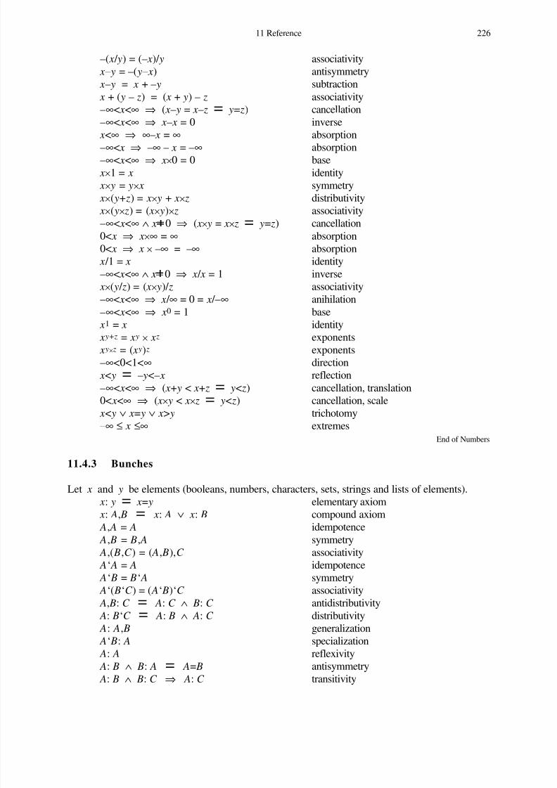
8/8/2019 37997710 Hehner a Practical Theory of Programming 2004
http://slidepdf.com/reader/full/37997710-hehner-a-practical-theory-of-programming-2004 233/242
–( x / y) = (– x)/ y associativity
x– y = –( y– x) antisymmetry
x– y = x + – y subtraction
x + ( y – z) = ( x + y) – z associativity
–∞< x<∞ ⇒ ( x– y = x– z = y= z) cancellation
–∞< x<∞ ⇒ x– x = 0 inverse
x<∞ ⇒ ∞– x = ∞ absorption–∞< x ⇒ –∞ – x = –∞ absorption
–∞< x<∞ ⇒ x×0 = 0 base
x×1 = x identity
x× y = y× x symmetry
x×( y+ z) = x× y + x× z distributivity
x×( y× z) = ( x× y)× z associativity
–∞< x<∞ ∧ x 0 ⇒ ( x× y = x× z = y= z) cancellation
0< x ⇒ x×∞ = ∞ absorption
0< x ⇒ x × –∞ = –∞ absorption
x /1 = x identity
–∞< x<∞ ∧ x 0 ⇒ x / x = 1 inverse x×( y / z) = ( x× y)/ z associativity
–∞< x<∞ ⇒ x / ∞ = 0 = x /–∞ anihilation
–∞< x<∞ ⇒ x0 = 1 base
x1 = x identity
x y+ z = x y × x z exponents
x y× z = ( x y) z exponents
–∞<0<1<∞ direction
x< y = – y<– x reflection
–∞< x<∞ ⇒ ( x+ y < x+ z = y< z) cancellation, translation
0< x<∞ ⇒ ( x× y < x× z = y< z) cancellation, scale
x< y ∨ x= y ∨ x> y trichotomy–∞ ≤ x ≤∞ extremes
End of Numbers
11.4.3 Bunches
Let x and y be elements (booleans, numbers, characters, sets, strings and lists of elements).
x: y = x= y elementary axiom
x: A, B = x: A ∨ x: B compound axiom
A, A = A idempotence
A, B = B, A symmetry
A,( B,C ) = ( A, B),C associativity A‘ A = A idempotence
A‘ B = B‘ A symmetry
A‘( B‘C ) = ( A‘ B)‘C associativity
A, B: C = A: C ∧ B: C antidistributivity
A: B‘C = A: B ∧ A: C distributivity
A: A, B generalization
A‘ B: A specialization
A: A reflexivity
A: B ∧ B: A = A= B antisymmetry
A: B ∧ B: C ⇒ A: C transitivity
11 Reference 226

8/8/2019 37997710 Hehner a Practical Theory of Programming 2004
http://slidepdf.com/reader/full/37997710-hehner-a-practical-theory-of-programming-2004 234/242
¢ null = 0 size
¢ x = 1 size
¢( A, B) + ¢( A‘ B) = ¢ A + ¢ B size
¬ x: A ⇒ ¢( A‘ x) = 0 size
A: B ⇒ ¢ A ≤ ¢ B size
A,( A‘ B) = A absorption
A‘( A, B) = A absorption A: B = A, B = B = A = A‘ B inclusion
A,( B,C ) = ( A, B),( A,C ) distributivity
A,( B‘C ) = ( A, B)‘( A,C ) distributivity
A‘( B,C ) = ( A‘ B), ( A‘C ) distributivity
A‘( B‘C ) = ( A‘ B)‘( A‘C ) distributivity
A: B ∧ C : D ⇒ A,C : B, D conflation, monotonicity
A: B ∧ C : D ⇒ A‘C : B‘ D conflation, monotonicity
null: A induction
A, null = A identity
A ‘ null = null base
¢ A = 0 = A = null sizei: x,.. y = x≤i< y (for extended integers i , x , y , x≤ y )
¢( x,.. y) = y– x (for extended integers x , y , x≤ y )
–null = null distribution
–( A, B) = – A, – B distribution
A+null = null+ A = null distribution
( A, B)+(C , D) = A+C , A+ D, B+C , B+ D distribution
and similarly for many other operators (see the final page of the book)
End of Bunches
11.4.4 Sets
{ A} A ${ A} = ¢ A~{ A} = A { A} { B} = { A, B}
A { B} = A: B { A} { B} = { A ‘ B}
{ A} { B} = A: B { A} = { B} = A = B{ A} 2
{ B} = A: B { A} { B} = A B End of Sets
11.4.5 Strings
Let S , T , and U be strings; let i and j be items (booleans, numbers, characters, bunch of
items, sets, lists, functions); let n be natural; let x , y , and z be integers.nil; S = S; nil = S S; (T ; U ) = (S; T ); U
nil = 0 i = 1
(S; T ) = S + T Snil = nil(S; i; T ) S = i ST ; U = ST ; SU S(T U )
= (ST )U 0*S = nil(n+1)*S = n*S; S i= j = S; i; T = S; j; T i< j ⇒ S; i; T < S; j; U nil ≤ S < S; i; T x;.. x = nil x;.. x+1 = x( x;.. y) ; ( y;.. z) = x;.. z ( x;.. y) = y– x
End of Strings
227 11 Reference
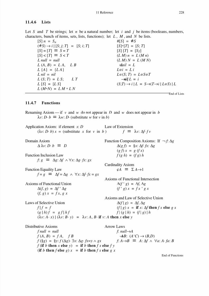
8/8/2019 37997710 Hehner a Practical Theory of Programming 2004
http://slidepdf.com/reader/full/37997710-hehner-a-practical-theory-of-programming-2004 235/242
11.4.6 Lists
Let S and T be strings; let n be a natural number; let i and j be items (booleans, numbers,
characters, bunch of items, sets, lists, functions); let L , M , and N be lists.
[S] n = Sn #[S] = S( S) → i | [S; j; T ] = [S; i; T ] [S]+[T ] = [S; T ]
[S] = [T ] = S = T [S] [T ] = [ST ][S] < [T ] = S < T ( L M ) n = L ( M n)
L null = null ( L M ) N = L ( M N ) L ( A, B) = L A, L B L@nil = L L { A} = { L A} L@i = L i L nil = nil L@(S; T ) = L@S@T L (S; T ) = L S; L T nil→i | L = i L [S] = [ L S] (S;T ) → i | L = S→(T →i | L@S) | L L ( M + N ) = L M + L N
End of Lists
11.4.7 Functions
Renaming Axiom — if v and w do not appear in D and w does not appear in bλv: D· b = λw: D· (substitute w for v in b)
Application Axiom: if element x: D Law of Extension
(λv: D· b) x = (substitute x for v in b ) f = λv: ∆ f · f v
Domain Axiom Function Composition Axioms: If ¬ f : ∆g∆ λv: D· b = D ∆(g f ) = § x: ∆ f · fx: ∆g
(g f ) x = g ( f x)
Function Inclusion Law f (g h) = ( f g) h f : g = ∆g: ∆ f ∧ ∀ x: ∆g· fx: gx
Cardinality Axiom
Function Equality Law ¢ A = Σ A→1
f = g = ∆ f = ∆g ∧ ∀ x: ∆ f · fx = gxAxioms of Functional Intersection
Axioms of Functional Union ∆( f ‘ g) = ∆ f , ∆g∆( f , g) = ∆ f ‘ ∆g ( f ‘ g) x = f x ‘ g x( f , g) x = f x, g x
Axioms and Law of Selective Union
Laws of Selective Union ∆( f | g) = ∆ f , ∆g
f | f = f ( f | g) x = if x: ∆ f then f x else g x(g | h) f = g f | h f f | (g | h) = ( f | g) | h(λv: A· x) | (λv: B· y) = λv: A, B· if v: A then x else y
Distributive Axioms Arrow Laws
f null = null f : null→ A f ( A, B) = f A, f B A→ B: ( A‘C ) → ( B, D)
f (§g) = § y: f (∆g)· ∃ x: ∆g· fx= y ∧ gx f : A→ B = A: ∆ f ∧ ∀a: A· fa: B f (if b then x else y) = if b then f x else f y(if b then f else g) x = if b then f x else g x
End of Functions
11 Reference 228
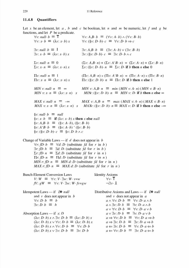
8/8/2019 37997710 Hehner a Practical Theory of Programming 2004
http://slidepdf.com/reader/full/37997710-hehner-a-practical-theory-of-programming-2004 236/242
11.4.8 Quantifiers
Let x be an element, let a , b and c be boolean, let n and m be numeric, let f and g be
functions, and let P be a predicate.
∀v: null· b = ∀v: A, B· b = (∀v: A· b) ∧ (∀v: B· b)
∀v: x· b = (λv: x· b) x ∀v: (§v: D· b)· c = ∀v: D· b ⇒ c
∃v: null· b = ∃v: A, B· b = (∃v: A· b) ∨ (∃v: B· b)
∃v: x· b = (λv: x· b) x ∃v: (§v: D· b)· c = ∃v: D· b ∧ c
Σv: null· n = 0 (Σv: A, B· n) + (Σv: A‘ B· n) = (Σv: A· n) + (Σv: B· n)
Σv: x· n = (λv: x· n) x Σv: (§v: D· b)· n = Σv: D· if b then n else 0
Πv: null· n = 1 (Πv: A, B· n) × (Πv: A‘ B· n) = (Πv: A· n) × (Πv: B· n)
Πv: x· n = (λv: x· n) x Πv: (§v: D· b)· n = Πv: D· if b then n else 1
MIN v: null· n = ∞ MIN v: A, B· n = min ( MIN v: A· n) ( MIN v: B· n)
MIN v: x· n = (λv: x· n) x MIN v: (§v: D· b)· n = MIN v: D· if b then n else ∞
MAX v: null· n = –∞ MAX v: A, B· n = max ( MAX v: A· n) ( MAX v: B· n)
MAX v: x· n = (λv: x· n) x MAX v: (§v: D· b)· n = MAX v: D· if b then n else –∞
§v: null· b = null§v: x· b = if (λv: x· b) x then x else null§v: A, B· b = (§v: A· b), (§v: B· b)
§v: A‘ B· b = (§v: A· b) ‘ (§v: B· b)
§v: (§v: D· b)· c = §v: D· b ∧ c
Change of Variable Laws — if d does not appear in b∀r : fD· b = ∀d : D· (substitute fd for r in b )
∃r : fD· b = ∃d : D· (substitute fd for r in b )
Σr : fD· n = Σd : D· (substitute fd for r in n )
Πr : fD· n = Πd : D· (substitute fd for r in n )
MIN r : fD· n = MIN d : D· (substitute fd for r in n )
MAX r : fD· n = MAX d : D· (substitute fd for r in n )
Bunch-Element Conversion Laws Identity Axioms
V : W = ∀v: V · ∃w: W · v=w ∀v·
fV : gW = ∀v: V · ∃w: W · fv=gw ¬∃v·
Idempotent Laws — if D null Distributive Axioms and Laws — if D nulland v does not appear in b and v does not appear in a∀v: D· b = b a ∧ ∀v: D· b = ∀v: D· a ∧ b∃v: D· b = b a ∧ ∃v: D· b = ∃v: D· a ∧ b
a ∨ ∀v: D· b = ∀v: D· a ∨ bAbsorption Laws — if x: D a ∨ ∃v: D· b = ∃v: D· a ∨ b
(λv: D· b) x ∧ ∃v: D· b = (λv: D· b) x a ⇒ ∀v: D· b = ∀v: D· a ⇒ b(λv: D· b) x ∨ ∀v: D· b = (λv: D· b) x a ⇒ ∃v: D· b = ∃v: D· a ⇒ b(λv: D· b) x ∧ ∀v: D· b = ∀v: D· b a ⇐ ∃v: D· b = ∀v: D· a ⇐ b(λv: D· b) x ∨ ∃v: D· b = ∃v: D· b a ⇐ ∀v: D· b = ∃v: D· a ⇐ b
229 11 Reference

8/8/2019 37997710 Hehner a Practical Theory of Programming 2004
http://slidepdf.com/reader/full/37997710-hehner-a-practical-theory-of-programming-2004 237/242
Specialization Law — if x: D Generalization Law — if x: D∀v: D· b ⇒ (λv: D· b) x (λv: D· b) x ⇒ ∃v: D· b
One-Point Laws — if x: D Splitting Laws — for any fixed domainand v does not appear in x ∀v· a ∧ b = (∀v· a) ∧ (∀v· b)∀v: D· v= x ⇒ b = (λv: D· b) x ∃v· a ∧ b ⇒ (∃v· a) ∧ (∃v· b)∃v: D· v= x ∧ b = (λv: D· b) x ∀v· a ∨ b ⇐ (∀v· a) ∨ (∀v· b)
∃v· a ∨ b = (∃v· a) ∨ (∃v· b)Duality Laws ∀v· a ⇒ b ⇒ (∀v· a) ⇒ (∀v· b)
¬∀v· b = ∃v· ¬b (deMorgan) ∀v· a ⇒ b ⇒ (∃v· a) ⇒ (∃v· b)¬∃v· b = ∀v· ¬b (deMorgan) ∀v· a = b ⇒ (∀v· a) = (∀v· b)– MAX v· n = MIN v· –n ∀v· a = b ⇒ (∃v· a) = (∃v· b)– MIN v· n = MAX v· –n
Commutative LawsSolution Laws ∀v· ∀w· b = ∀w· ∀v· b
§v: D· = D ∃v· ∃w· b = ∃w· ∃v· b(§v: D· b): D§v: D· = null Semicommutative Laws (Skolem)(§v· b): (§v· c)
= ∀v· b⇒c ∃v· ∀w· b ⇒ ∀w· ∃v· b
(§v· b), (§v· c) = §v· b ∨ c ∀ x· ∃ y· Pxy = ∃ f · ∀ x· Px( fx)(§v· b) ‘ (§v· c) = §v· b ∧ c x: § p = x: ∆ p ∧ px Domain Change Laws∀ f = (§ f )=(∆ f ) A: B ⇒ (∀v: A· b) ⇐ (∀v: B· b)∃ f = (§ f ) null A: B ⇒ (∃v: A· b) ⇒ (∃v: B· b)
∀v: A· v: B ⇒ p = ∀v: A‘ B· pBounding Axioms and Laws ∃v: A· v: B ∧ p = ∃v: A‘ B· p
if v does not appear in nn > ( MAX v: D· m) ⇒ (∀v: D· n>m) Extreme Lawn < ( MIN v: D· m) ⇒ (∀v: D· n<m) ∀v· ( MIN v· n) ≤ n ≤ ( MAX v· n)n ≥ ( MAX v: D· m) = (∀v: D· n≥m)
n ≤ ( MIN v: D· m) = (∀v: D· n≤m) Connection Laws (Galois)n ≥ ( MIN v: D· m) ⇐ (∃v: D· n≥m) n≤m = ∀k · k ≤n ⇒ k ≤mn ≤ ( MAX v: D· m) ⇐ (∃v: D· n≤m) n≤m = ∀k · k <n ⇒ k <mn > ( MIN v: D· m) = (∃v: D· n>m) n≤m = ∀k · m≤k ⇒ n≤k n < ( MAX v: D· m) = (∃v: D· n<m) n≤m = ∀k · m<k ⇒ n<k
Distributive Laws — if D null and v does not appear in nmax n ( MAX v: D· m) = ( MAX v: D· max n m)max n ( MIN v: D· m) = ( MIN v: D· max n m)min n ( MAX v: D· m) = ( MAX v: D· min n m)min n ( MIN v: D· m) = ( MIN v: D· min n m)n + ( MAX v: D· m) = ( MAX v: D· n+m)
n + ( MIN v: D· m) = ( MIN v: D· n+m)n – ( MAX v: D· m) = ( MIN v: D· n–m)n – ( MIN v: D· m) = ( MAX v: D· n–m)( MAX v: D· m) – n = ( MAX v: D· m–n)( MIN v: D· m) – n = ( MIN v: D· m–n)n≥0 ⇒ n × ( MAX v: D· m) = ( MAX v: D· n×m)n≥0 ⇒ n × ( MIN v: D· m) = ( MIN v: D· n×m)n≤0 ⇒ n × ( MAX v: D· m) = ( MIN v: D· n×m)n≤0 ⇒ n × ( MIN v: D· m) = ( MAX v: D· n×m)n × (Σv: D· m) = (Σv: D· n×m)(Πv: D· m)n = (Πv: D· mn)
End of Quantifiers
11 Reference 230

8/8/2019 37997710 Hehner a Practical Theory of Programming 2004
http://slidepdf.com/reader/full/37997710-hehner-a-practical-theory-of-programming-2004 238/242
11.4.9 Limits
( MAX m· MIN n· f (m+n)) ≤ ( LIM f ) ≤ ( MIN m· MAX n· f (m+n))
∃m· ∀n· p(m+n) ⇒ LIM p ⇒ ∀m· ∃n· p(m+n)
End of Limits
11.4.10 Specifications and Programs
For specifications P , Q , R , and S , and boolean b ,
ok = x′= x ∧ y′= y ∧ ...
x:= e = x′=e ∧ y′= y ∧ ...
P. Q = ∃ x′′, y′′, ...· (substitute x′′ for x′ , y′′ for y′ , ... in P )
∧ (substitute x′′ for x , y′′ for y , ... in Q )
P||Q = ∃t P, t Q· (substitute t P for t ′ in P )
∧ (substitute t Q for t ′ in Q )
∧ t ′ = max t P t Qif b then P else Q = b ∧ P ∨ ¬b ∧ Q
var x: T · P = ∃ x, x′: T · Pwhile b do P = t ′≥t ∧ (if b then (P. t := t +inc. while b do P) else ok )
(Fmn ⇐ m=n ∧ ok ) ∧ (Fik ⇐ m≤i< j<k ≤n ∧ (Fij. Fjk ))⇒ (Fmn ⇐ for i:= m;..n do m≤i<n ⇒ Fi(i+1))
Im⇒ I ′n ⇐ for i:= m;..n do m≤i<n ∧ Ii ⇒ I ′(i+1)
wait until w = t := max t wassert b = if b then ok else ( print "error". wait until ∞)
ensure b = b ∧ ok x′ = (P result e) = P. x′ = ec? = r := r +1
c = M (r –1)
c! e = M w = e ∧ T w = t ∧ (w:= w+1)√c = T r + (transit time) ≤ t ivar x: T · S = ∃ x: time→T · Schan c: T · P = ∃M c: [∞*T ]· ∃T c: [∞* xreal]· var r c , wc: xnat := 0· Pok. P = P. ok = P identity
P. (Q. R) = (P. Q). R associativity
if b then P else P = P idempotence
if b then P else Q = if ¬b then Q else P case reversal
P = if b then b ⇒ P else ¬b ⇒ P case creation
P∨Q. R∨S = (P. R) ∨ (P. S) ∨ (Q. R) ∨ (Q. S) distributivity
(if b then P else Q). R = if b then (P. R) else (Q. R) distributivity (unprimed b )
ok || P = P || ok = P identityP || Q = Q || P symmetry
P || (Q || R) = (P || Q) || R associativity
P || Q∨ R = (P || Q) ∨ (P || R) distributivity
P || if b then Q else R = if b then (P || Q) else (P || R) distributivity
if b then (P||Q) else ( R||S) = if b then P else R || if b then Q else S distributivity
x:= if b then e else f = if b then x:= e else x:= f functional-imperative
∀σ, σ′· (if b then (P. W ) else ok ⇐ W ) ⇒ ∀σ, σ′· (while b do P ⇐ W ) End of Specifications and Programs
231 11 Reference

8/8/2019 37997710 Hehner a Practical Theory of Programming 2004
http://slidepdf.com/reader/full/37997710-hehner-a-practical-theory-of-programming-2004 239/242
11.4.11 Substitution
Let x and y be different boundary state variables, let e and f be expressions of the prestate,
and let P be a specification.
x:= e. P = (for x substitute e in P )
( x:= e || y:= f ). P = (for x substitute e and independently for y substitute f in P )
End of Substitution
11.4.12 Conditions
Let P and Q be any specifications, and let C be a precondition, and let C ′ be the corresponding
postcondition (in other words, C ′ is the same as C but with primes on all the state variables).
C ∧ (P. Q) ⇐ C ∧P. QC ⇒ (P.Q) ⇐ C ⇒P. Q(P.Q) ∧ C ′ ⇐ P. Q∧C ′(P.Q) ⇐ C ′ ⇐ P. Q⇐C ′P. C ∧Q ⇐ P∧C ′. Q
P. Q ⇐ P∧C ′. C ⇒QC is a sufficient precondition for P to be refined by S
if and only if C ⇒P is refined by S .
C ′ is a sufficient postcondition for P to be refined by Sif and only if C ′⇒P is refined by S .
End of Conditions
11.4.13 Refinement
Refinement by Steps (Stepwise Refinement) (monotonicity, transitivity)
If A ⇐ if b then C else D and C ⇐ E and D ⇐ F are theorems,
then A ⇐ if b then E else F is a theorem.If A ⇐ B.C and B ⇐ D and C ⇐ E are theorems, then A ⇐ D. E is a theorem.
If A ⇐ B||C and B ⇐ D and C ⇐ E are theorems, then A ⇐ D|| E is a theorem.
If A ⇐ B and B ⇐ C are theorems, then A ⇐ C is a theorem.
Refinement by Parts (monotonicity, conflation)
If A ⇐ if b then C else D and E ⇐ if b then F else G are theorems,
then A∧ E ⇐ if b then C ∧F else D∧G is a theorem.
If A ⇐ B.C and D ⇐ E .F are theorems, then A∧ D ⇐ B∧ E . C ∧F is a theorem.
If A ⇐ B||C and D ⇐ E ||F are theorems, then A∧ D ⇐ B∧ E || C ∧F is a theorem.
If A ⇐ B and C ⇐ D are theorems, then A∧C ⇐ B∧ D is a theorem.
Refinement by Cases
P ⇐ if b then Q else R is a theorem if and only if
P ⇐ b ∧ Q and P ⇐ ¬b ∧ R are theorems.
End of Refinement
End of Laws
11 Reference 232

8/8/2019 37997710 Hehner a Practical Theory of Programming 2004
http://slidepdf.com/reader/full/37997710-hehner-a-practical-theory-of-programming-2004 240/242
11.5 Names
abs: xreal→§r : xreal· r ≥0 abs r = if r ≥0 then r else –r bool (the booleans) bool = ,
ceil: real→int r ≤ ceil r < r +1
char (the characters) char = ..., `a, `A, ...
div: real→(§r : real· r >0)→int div x y = floor ( x / y)divides: (nat +1)→int →bool divides n i = i / n: int entro: prob→§r : xreal· r ≥0 entro p = p × info p + (1– p) × info (1– p)
even: int →bool even i = i /2: int even = divides 2
floor : real→int floor r ≤ r < floor r + 1
info: prob→§r : xreal· r ≥0 info p = – log pint (the integers) int = nat , –nat LIM (limit quantifier) see Axioms and Laws
log: (§r : xreal· r ≥0)→ xreal log(2 x) = xlog ( x× y) = log x + log y
max: xrat → xrat → xrat max x y= if x≥ y then x else y– max a b = min (–a) (–b)
MAX (maximum quantifier) see Axioms and Laws
min: xrat → xrat → xrat min x y= if x≤ y then x else y– min a b = max (–a) (–b)
MIN (minimum quantifier) see Axioms and Laws
mod : real→(§r : real· r >0)→real 0 ≤ mod a d < d a = div a d × d + mod a d
nat (the naturals) 0, nat +1: nat 0, B+1: B ⇒ nat : B
nil (the empty string) nil = 0
nil; S = S = S; nilnil ≤ S
null (the empty bunch) ¢null = 0
null, A = A = A, nullnull: A
odd : int →bool odd i = ¬ i /2: int odd = ¬even
ok (the empty program) ok = σ′=σok .P = P.ok = ok || P = P || ok = P
prob (probability) prob = §r : real· 0≤r ≤1
rand (random number) rand n: 0,..n
rat (the rationals) rat = int /(nat +1)real (the reals) r : real = r : xreal ∧ –∞<r <∞suc: nat →(nat +1) suc n = n+1
xint (the extended integers) xint = –∞, int , ∞ xnat (the extended naturals) xnat = nat , ∞ xrat (the extended rationals) xrat = –∞, rat , ∞ xreal (the extended reals) x: xreal = ∃ f : nat →rat · x = LIM f End of Names
233 11 Reference

8/8/2019 37997710 Hehner a Practical Theory of Programming 2004
http://slidepdf.com/reader/full/37997710-hehner-a-practical-theory-of-programming-2004 241/242
11.6 Symbols
3 true ( ) 4 parentheses for grouping
3 false { } 17 set brackets
¬ 3 not [ ] 20 list brackets
∧ 3 and 2 17 powerset
∨ 3 or ¢ 14 bunch size, cardinality⇒ 3 implies $ 17 set size, cardinality
⇒ 3 implies 18 string size, length
⇐ 3 follows from, is implied by # 20 list size, length
⇐ 3 follows from, is implied by | 20,24 selective union, otherwise
= 3 equals, if and only if || 118 indep't (parallel) composition
= 3 equals, if and only if ~ 17 contents of a set
3 differs from, is unequal to * 18 repetition of a string
< 13 less than ∆ 23 domain of a function
> 13 greater than → 25 function arrow
≤ 13 less than or equal to 17 element of a set
≥ 13 greater than or equal to 17 subset+ 12 plus 17 set union+ 20 list catenation 17 set intersection
– 12 minus @ 22 index with a pointer
× 12 times, multiplication λ 23 function, variable introduction
/ 12 divided by ∀ 26 for all, universal quantifier
, 14 bunch union ∃ 26 there exists, existential quantifier
, . . 16 union from (incl) to (excl) Σ 26 sum of, summation quantifier
‘ 14 bunch intersection Π 26 product of, product quantifier
; 17 string catenation § 27 those, solution quantifier
; .. 19 catenation from (incl) to (excl) ′ 34 x′ is final value of state var x
: 14 is in, bunch inclusion ` 13 `A is a character:: 90 includes " 21 "hello" is a text or list of chars
:= 36 assignment ab 12 exponentiation
. 36 dep't (sequential) composition ab 18 string indexing
· 23 variable introduction a b 20,31 indexing,application,composition
! 133 output √ 133 input check
? 133 input ∞ 12 infinity
assert 77 ivar 126
chan 138 loop end 71
ensure 77 or 77
exit when 71 result 78for do 74 var 66
frame 67 wait until 76
go to 76 while do 69
if then else 4
End of Symbols
11 Reference 234

8/8/2019 37997710 Hehner a Practical Theory of Programming 2004
http://slidepdf.com/reader/full/37997710-hehner-a-practical-theory-of-programming-2004 242/242
11.7 Precedence
0. ( ) { } [ ] loop end numbers characters texts names
1. @ juxtaposition
2. +prefix –prefix ¢ $ # * ~ 2 ∆ → superscript subscript
3. × /
4. + –+
5. ; ;.. ‘
6. , ,.. |7. = < > ≤ ≥ : ::
235 11 Reference


![[Practical] Functional Programming in Rails](https://img.pdfslide.us/doc/110x75/53fda89c8d7f72a81c8b4a44/practical-functional-programming-in-rails.jpg)