Embed Size (px)
Citation preview

© W. Venables, 2003
Data Analysis & Graphics 1
CS
IRO
Math
em
atica
l an
d In
form
atio
n S
cien
ces
Statistical Models in S
The template is a multiple linear regression model:
In matrix terms this would be written
where• y is the response vector,
• β is the vector of regression coefficients,
• X is the model matrix or design matrix and
• e is the error vector.
2
1
where NID(0, )p
i ij j i ij
y x e e
y X e
© W. Venables, 2003
Data Analysis & Graphics 2
CS
IRO
Math
em
atica
l an
d In
form
atio
n S
cien
ces
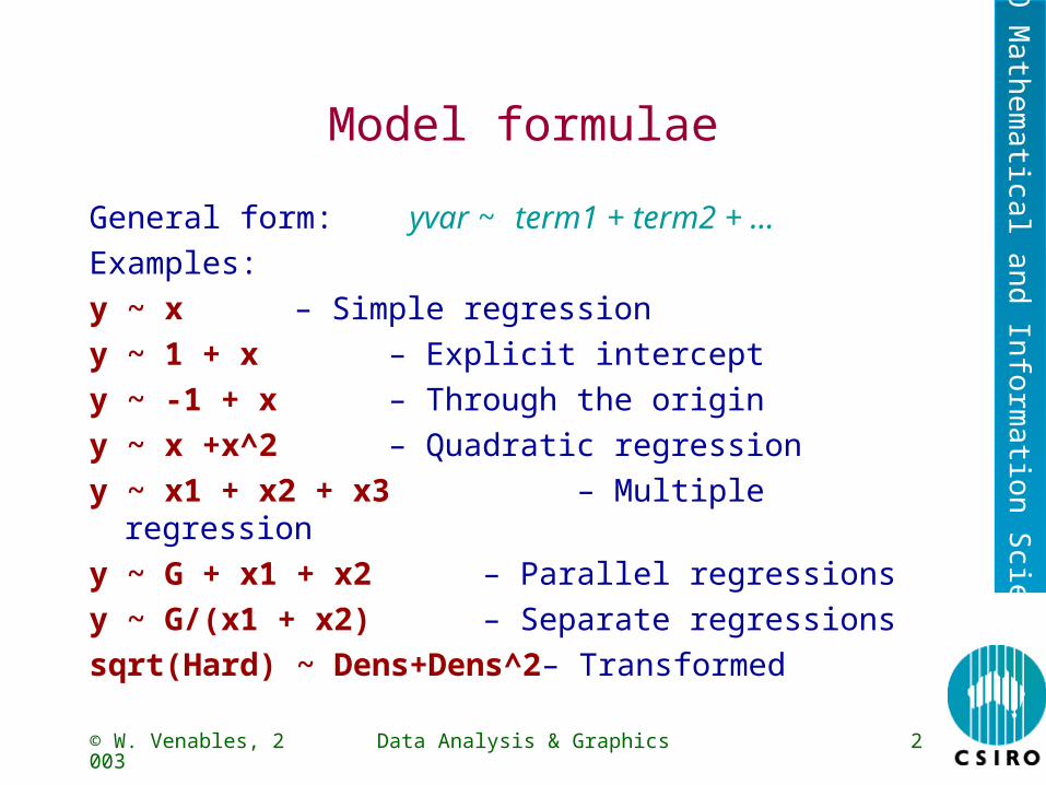
Model formulae
General form: yvar ~ term1 + term2 + … Examples:y ~ x – Simple regressiony ~ 1 + x – Explicit intercepty ~ -1 + x – Through the originy ~ x +x^2 – Quadratic regressiony ~ x1 + x2 + x3 – Multiple regressiony ~ G + x1 + x2 – Parallel regressionsy ~ G/(x1 + x2) – Separate regressionssqrt(Hard) ~ Dens+Dens^2– Transformed

© W. Venables, 2003
Data Analysis & Graphics 3
CS
IRO
Math
em
atica
l an
d In
form
atio
n S
cien
ces
More examples of formulae
y ~ G – Single classification
y ~ A + B – Randomized block
y ~ B + N*P – Factorial in blocks
y ~ x + B + N*P – with covariate
y ~ . - X1 – All variables except X1
. ~ . + A:B – Add interaction (update)
Nitrogen ~ Times*(River/Site) - more complex design

© W. Venables, 2003
Data Analysis & Graphics 4
CS
IRO
Math
em
atica
l an
d In
form
atio
n S
cien
ces
Generic functions for inference
The following apply to most modelling objects
coef(obj) regression coefficients
resid(obj) residuals
fitted(obj) fitted values
summary(obj) analysis summary
predict(obj,newdata = ndat) predict for new data
deviance(obj) residual sum of squares

© W. Venables, 2003
Data Analysis & Graphics 5
CS
IRO
Math
em
atica
l an
d In
form
atio
n S
cien
ces
Example: The Janka data
Hardness and density data for 36 samples of Australian hardwoods.
Source: E. J. Williams, “Regression Analysis”, Wiley, 1959. [ex-CSIRO, Forestry.]
Problem: build a prediction model for Hardness using Density.

© W. Venables, 2003
Data Analysis & Graphics 6
CS
IRO
Math
em
atica
l an
d In
form
atio
n S
cien
ces5
00
10
00
15
00
20
00
25
00
30
00
30 40 50 60 70
Density
Ha
rdn
ess
The Janka data. Hardness and densityof 36 species of Australian hardwoodsamples

© W. Venables, 2003
Data Analysis & Graphics 7
CS
IRO
Math
em
atica
l an
d In
form
atio
n S
cien
ces
Janka data - initial model building
We might start with a linear or quadratic model (suggested by Williams) and start checking the fit.
> jank.1 <- lm(Hard ~ Dens, janka)
> jank.2 <- update(jank.1, . ~ . + Dens^2)
> summary(jank.2)$coef
Value Std. Error t value Pr(>|t|)
(Intercept) -118.00738 334.96690 -0.35230 0.726857
Dens 9.43402 14.93562 0.63165 0.531970
I(Densˆ2) 0.50908 0.15672 3.24830 0.002669
© W. Venables, 2003
Data Analysis & Graphics 8
CS
IRO
Math
em
atica
l an
d In
form
atio
n S
cien
ces
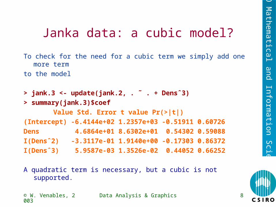
Janka data: a cubic model?
To check for the need for a cubic term we simply add one more term
to the model
> jank.3 <- update(jank.2, . ˜ . + Densˆ3)
> summary(jank.3)$coef
Value Std. Error t value Pr(>|t|)
(Intercept) -6.4144e+02 1.2357e+03 -0.51911 0.60726
Dens 4.6864e+01 8.6302e+01 0.54302 0.59088
I(Densˆ2) -3.3117e-01 1.9140e+00 -0.17303 0.86372
I(Densˆ3) 5.9587e-03 1.3526e-02 0.44052 0.66252
A quadratic term is necessary, but a cubic is not supported.

© W. Venables, 2003
Data Analysis & Graphics 9
CS
IRO
Math
em
atica
l an
d In
form
atio
n S
cien
ces
Janka data - stability of coefficients
The regression coefficients should remain more stable under extensions to the model if we standardize, or even just mean-correct, the predictors:
> janka$d <- scale(janka$Dens, scale=F)
> jank.1 <- lm(Hard ~ d, janka)
> jank.2 <- update(jank.1, .~.+d^2)
> jank.3 <- update(jank.2, .~.+d^3)

© W. Venables, 2003
Data Analysis & Graphics 10
CS
IRO
Math
em
atica
l an
d In
form
atio
n S
cien
ces
summary(jank.1)$coef Value Std. Error t value Pr(>|t|) (Intercept) 1469.472 30.5099 48.164 0 d 57.507 2.2785 25.238 0> summary(jank.2)$coef Value Std. Error t value Pr(>|t|) (Intercept) 1378.19661 38.93951 35.3933 0.000000 d 55.99764 2.06614 27.1026 0.000000 I(d^2) 0.50908 0.15672 3.2483 0.002669> round(summary(jank.3)$coef, 4) Value Std. Error t value Pr(>|t|) (Intercept) 1379.1028 39.4775 34.9339 0.0000 d 53.9610 5.0746 10.6336 0.0000 I(d^2) 0.4864 0.1668 2.9151 0.0064 I(d^3) 0.0060 0.0135 0.4405 0.6625Why is this so? Does it matter very much?

© W. Venables, 2003
Data Analysis & Graphics 11
CS
IRO
Math
em
atica
l an
d In
form
atio
n S
cien
ces
Checks and balances
> xyplot(studres(janka.lm2) ~ fitted(janka.lm2),
panel = function(x, y, ...) {
panel.xyplot(x, y, col = 5, ...)
panel.abline(h = 0, lty = 4, col = 6)
}, xlab = "Fitted values", ylab = "Residuals")
> qqmath(~ studres(janka.lm2), panel = function(x, y, ...) {
panel.qqmath(x, y, col = 5, ...)
panel.qqmathline(y, qnorm, col = 4)
}, xlab = "Normal scores",
ylab = "Sorted studentized residuals")

© W. Venables, 2003
Data Analysis & Graphics 12
CS
IRO
Math
em
atica
l an
d In
form
atio
n S
cien
ces
-2
0
2
4
500 1000 1500 2000 2500 3000
Fitted values
Re
sid
ua
ls
Janka data:Studentized residualsagainst fitted values forthe quadratic model

© W. Venables, 2003
Data Analysis & Graphics 13
CS
IRO
Math
em
atica
l an
d In
form
atio
n S
cien
ces
-2
0
2
4
-2 -1 0 1 2
Normal scores
So
rte
d s
tud
en
tize
d r
esi
du
als
Janka data:Sorted studentized residualsagainst normal scores for the quadratic model

© W. Venables, 2003
Data Analysis & Graphics 14
CS
IRO
Math
em
atica
l an
d In
form
atio
n S
cien
ces
Janka data - trying a transformation
The Box-Cox family of transformations includes square-root and log transformations as special cases.
The boxcox function in the MASS library allows the marginal likelihood function for the transformation parameter to be calculated and displayed. It’s use is easy. (Note: it only applies to positive response variables.)
> library(MASS, first = T)
> graphsheet() # necessary if no graphics device open.
> boxcox(jank.2,
lambda = seq(-0.25, 1, len=20))

© W. Venables, 2003
Data Analysis & Graphics 15
CS
IRO
Math
em
atica
l an
d In
form
atio
n S
cien
ces
lambda
log
-Lik
elih
oo
d
-0.2 0.0 0.2 0.4 0.6
-24
0-2
39
-23
8-2
37
95%
-0.1876 0.1500 0.5078
© W. Venables, 2003
Data Analysis & Graphics 16
CS
IRO
Math
em
atica
l an
d In
form
atio
n S
cien
ces
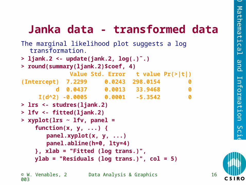
Janka data - transformed dataThe marginal likelihood plot suggests a log transformation.> ljank.2 <- update(jank.2, log(.)˜.)> round(summary(ljank.2)$coef, 4) Value Std. Error t value Pr(>|t|) (Intercept) 7.2299 0.0243 298.0154 0 d 0.0437 0.0013 33.9468 0 I(d^2) -0.0005 0.0001 -5.3542 0> lrs <- studres(ljank.2)> lfv <- fitted(ljank.2)> xyplot(lrs ~ lfv, panel = function(x, y, ...) {
panel.xyplot(x, y, ...) panel.abline(h=0, lty=4)
}, xlab = "Fitted (log trans.)", ylab = "Residuals (log trans.)", col = 5)

© W. Venables, 2003
Data Analysis & Graphics 17
CS
IRO
Math
em
atica
l an
d In
form
atio
n S
cien
ces
-2
-1
0
1
2
6.5 7.0 7.5 8.0
Fitted (log trans.)
Re
sid
ua
ls (
log
tra
ns.
)

© W. Venables, 2003
Data Analysis & Graphics 18
CS
IRO
Math
em
atica
l an
d In
form
atio
n S
cien
ces
Plot of transformed data> attach(janka)
> plot(Dens, Hard, log = "y")
Dens
Ha
rd
30 40 50 60 70
50
01
00
01
50
02
00
03
00
0

© W. Venables, 2003
Data Analysis & Graphics 19
CS
IRO
Math
em
atica
l an
d In
form
atio
n S
cien
ces
Selecting terms in a multiple regression
Example: The Iowa wheat data.> names(iowheat) [1] "Year" "Rain0" "Temp1" "Rain1" "Temp2" [6] "Rain2" "Temp3" "Rain3" "Temp4" "Yield"
> bigm <- lm(Yield ~ ., data = iowheat)
fits a regression model using all other variables in the data frame as predictors.
From the big model, now check the effect of dropping each term individually:

© W. Venables, 2003
Data Analysis & Graphics 20
CS
IRO
Math
em
atica
l an
d In
form
atio
n S
cien
ces
> dropterm(bigm, test = "F")
Single term deletions
Model:
Yield ~ Year + Rain0 + Temp1 + Rain1 + Temp2 + Rain2 +
Temp3 + Rain3 + Temp4
Df Sum of Sq RSS AIC F Value Pr(F)
<none> 1404.8 143.79
Year 1 1326.4 2731.2 163.73 21.715 0.00011
Rain0 1 203.6 1608.4 146.25 3.333 0.08092
Temp1 1 70.2 1475.0 143.40 1.149 0.29495
Rain1 1 33.2 1438.0 142.56 0.543 0.46869
Temp2 1 43.2 1448.0 142.79 0.707 0.40905
Rain2 1 209.2 1614.0 146.37 3.425 0.07710
Temp3 1 0.3 1405.1 141.80 0.005 0.94652
Rain3 1 9.5 1414.4 142.01 0.156 0.69655
Temp4 1 58.6 1463.5 143.14 0.960 0.33738

© W. Venables, 2003
Data Analysis & Graphics 21
CS
IRO
Math
em
atica
l an
d In
form
atio
n S
cien
ces
> smallm <- update(bigm, . ~ Year)> addterm(smallm, bigm, test = "F")Single term additions
Model:Yield ~ Year Df Sum of Sq RSS AIC F Value Pr(F) <none> 2429.8 145.87 Rain0 1 138.65 2291.1 145.93 1.8155 0.18793 Temp1 1 30.52 2399.3 147.45 0.3816 0.54141 Rain1 1 47.88 2381.9 147.21 0.6031 0.44349 Temp2 1 16.45 2413.3 147.64 0.2045 0.65437 Rain2 1 518.88 1910.9 139.94 8.1461 0.00775 Temp3 1 229.14 2200.6 144.60 3.1238 0.08733 Rain3 1 149.78 2280.0 145.77 1.9708 0.17063 Temp4 1 445.11 1984.7 141.19 6.7282 0.01454

© W. Venables, 2003
Data Analysis & Graphics 22
CS
IRO
Math
em
atica
l an
d In
form
atio
n S
cien
ces
Automated selection of variables
> stepm <- stepAIC(bigm, scope = list(lower = ~ Year))
Start: AIC= 143.79 ....Step: AIC= 137.13 Yield ~ Year + Rain0 + Rain2 + Temp4
Df Sum of Sq RSS AIC <none> NA NA 1554.6 137.13- Temp4 1 187.95 1742.6 138.90- Rain0 1 196.01 1750.6 139.05- Rain2 1 240.20 1794.8 139.87>

© W. Venables, 2003
Data Analysis & Graphics 23
CS
IRO
Math
em
atica
l an
d In
form
atio
n S
cien
ces
A Random Effects model
• The petroleum data of Nilon L Prater, (c. 1954).
• 10 crude oil sources, with measurements on the crude oil itself.
• Subsamples of crude (3-5) refined to a certain end point (measured).
• The response is the yield of refined petroleum (as a percentage).
• How can petroleum yield be predicted from properties of crude and end point?

© W. Venables, 2003
Data Analysis & Graphics 24
CS
IRO
Math
em
atica
l an
d In
form
atio
n S
cien
ces
A first look: Trellis display
For this kind of grouped data a Trellis display, by group,
with a simple model fitted within each group is often very revealing.
> names(petrol)
[1] "No" "SG" "VP" "V10" "EP" "Y"
> xyplot(Y ~ EP | No, petrol, as.table = T,
panel = function(x, y, ...) {
panel.xyplot(x, y, ...)
panel.lmline(x, y, ...)
}, xlab = "End point", ylab = "Yield (%)",
main = "Petroleum data of N L Prater")
>

© W. Venables, 2003
Data Analysis & Graphics 25
CS
IRO
Math
em
atica
l an
d In
form
atio
n S
cien
ces
10
20
30
40
A
200 250 300 350 400 450
B C
200 250 300 350 400 450
D
E F G
10
20
30
40
H
10
20
30
40
200 250 300 350 400 450
I J
End point
Yie
ld (
%)
Petroleum data of N L Prater

© W. Venables, 2003
Data Analysis & Graphics 26
CS
IRO
Math
em
atica
l an
d In
form
atio
n S
cien
ces
Fixed effect Models
Clearly a straight line model is reasonable. There is some variation between groups, but parallel lines
is also a reasonable simplification.There appears to be considerable variation between
intercepts, though.> pet.2 <- aov(Y ~ No*EP, petrol)> pet.1 <- update(pet.2, .~.-No:EP)> pet.0 <- update(pet.1, .~.-No)> anova(pet.0, pet.1, pet.2)Analysis of Variance Table
Response: Y
Terms Resid. Df RSS Test Df Sum of Sq F Value Pr(F) 1 EP 30 1759.7 2 No + EP 21 74.1 +No 9 1685.6 74.101 0.00003 No * EP 12 30.3 +No:EP 9 43.8 1.926 0.1439

© W. Venables, 2003
Data Analysis & Graphics 27
CS
IRO
Math
em
atica
l an
d In
form
atio
n S
cien
ces
Random effects
> pet.re1 <- lme(Y ~ EP, petrol, random = ~1+EP|No)> summary(pet.re1)..... AIC BIC logLik 184.77 193.18 -86.387
Random effects: Formula: ~ 1 + EP | No Structure: General positive-definite StdDev Corr (Intercept) 4.823890 (Inter EP 0.010143 1 Residual 1.778504
Fixed effects: Y ~ EP Value Std.Error DF t-value p-value (Intercept) -31.990 2.3617 21 -13.545 <.0001 EP 0.155 0.0062 21 24.848 <.0001 Correlation: .....
© W. Venables, 2003
Data Analysis & Graphics 28
CS
IRO
Math
em
atica
l an
d In
form
atio
n S
cien
ces
The shrinkage effect
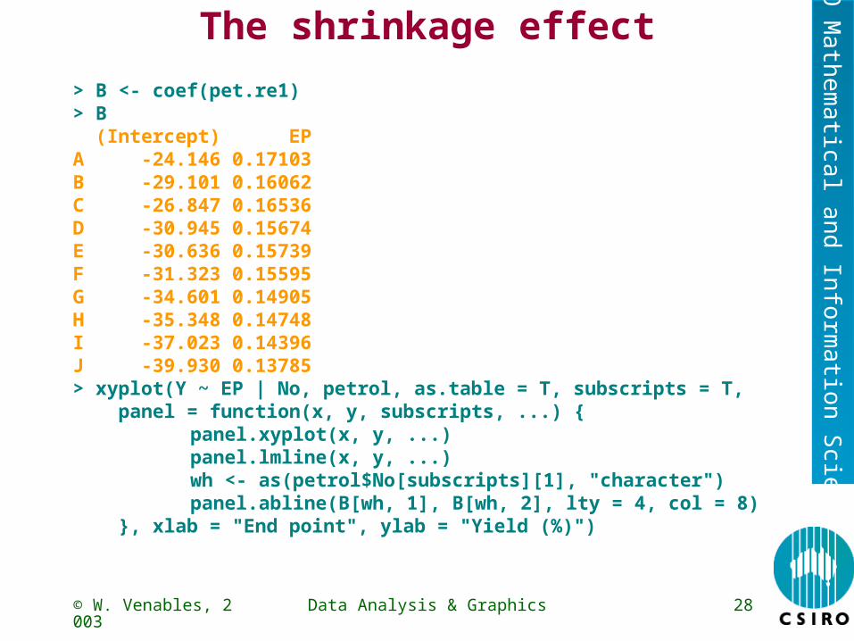
> B <- coef(pet.re1)> B (Intercept) EP A -24.146 0.17103B -29.101 0.16062C -26.847 0.16536D -30.945 0.15674E -30.636 0.15739F -31.323 0.15595G -34.601 0.14905H -35.348 0.14748I -37.023 0.14396J -39.930 0.13785> xyplot(Y ~ EP | No, petrol, as.table = T, subscripts = T, panel = function(x, y, subscripts, ...) { panel.xyplot(x, y, ...) panel.lmline(x, y, ...) wh <- as(petrol$No[subscripts][1], "character") panel.abline(B[wh, 1], B[wh, 2], lty = 4, col = 8) }, xlab = "End point", ylab = "Yield (%)")

© W. Venables, 2003
Data Analysis & Graphics 29
CS
IRO
Math
em
atica
l an
d In
form
atio
n S
cien
ces
10
20
30
40
A
200 250 300 350 400 450
B C
200 250 300 350 400 450
D
E F G
10
20
30
40
H
10
20
30
40
200 250 300 350 400 450
I J
End point
Yie
ld (
%)
Note how the random effect (red, broken) lines are less variable than the separate least squares lines.

© W. Venables, 2003
Data Analysis & Graphics 30
CS
IRO
Math
em
atica
l an
d In
form
atio
n S
cien
ces
General notes on modelling
1. Analysis of variance models are linear models but usually fitted using aov rather than lm. The computation is the same but the resulting object behaves differently in response to some generics, especially summary.
2. Generalized linear modelling (logistic regression, log-linear models, quasi-likelihood, &c) also use linear modelling formulae in that they specify the model matrix, not the parameters. Generalized additive modelling (smoothing splines, loess models, &c) formulae are quite similar.
3. Non-linear regression uses a formula, but a completely different paradigm: the formula gives the full model as an expression, including parameters.

© W. Venables, 2003
Data Analysis & Graphics 31
CS
IRO
Math
em
atica
l an
d In
form
atio
n S
cien
ces
GLMs and GAMs: An introduction
• One generalization of multiple linear regression.
• Response, y, stimulus variables
• The distribution of Y depends on the x's through a single linear
function, the 'linear predictor'
• There may be an unknown 'scale' (or 'variance') parameter to
estimate as well
• The deviance is a generalization of the residual sum of squares.
• The protocols are very similar to linear regression. The
inferential logic is virtually identical.
1 1 2 2 p px x x
1 2, ,..., px x x

© W. Venables, 2003
Data Analysis & Graphics 32
CS
IRO
Math
em
atica
l an
d In
form
atio
n S
cien
ces
Example: budworms (MASS, Ch. 7)
Classical toxicology study of budworms, by sex.
> Budworms <- data.frame(Logdose = rep(0:5, 2),
Sex = factor(rep(c("M", "F"), each = 6)),
Dead = c(1, 4, 9, 13, 18, 20, 0, 2, 6, 10, 12, 16))
> Budworms$Alive <- 20 - Budworms$Dead
> xyplot(Dead/20 ~ I(2^Logdose), Budworms,
groups = Sex, panel = panel.superpose,
xlab = "Dose", ylab = "Fraction dead",
key = list(......), type="b")

© W. Venables, 2003
Data Analysis & Graphics 33
CS
IRO
Math
em
atica
l an
d In
form
atio
n S
cien
ces
0.0
0.2
0.4
0.6
0.8
1.0
0 5 10 15 20 25 30
Dose
Fra
ctio
n d
ea
dFemales: Males:

© W. Venables, 2003
Data Analysis & Graphics 34
CS
IRO
Math
em
atica
l an
d In
form
atio
n S
cien
ces
Fitting a model and plotting the results
Fitting the model is similar to a linear model> bud.1 <- glm(cbind(Dead, Alive) ~ Sex*Logdose,
binomial, Budworms, trace=T, eps=1.0e-9)GLM linear loop 1: deviance = 5.0137 GLM linear loop 2: deviance = 4.9937 GLM linear loop 3: deviance = 4.9937 GLM linear loop 4: deviance = 4.9937 > summary(bud.1, cor = F)… Value Std. Error t value (Intercept) -2.99354 0.55270 -5.41622 Sex 0.17499 0.77831 0.22483 Logdose 0.90604 0.16710 5.42207Sex:Logdose 0.35291 0.26999 1.30713…(Residual Deviance: 4.9937 on 8 degrees of freedom

© W. Venables, 2003
Data Analysis & Graphics 35
CS
IRO
Math
em
atica
l an
d In
form
atio
n S
cien
ces
> bud.0 <- update(bud.1, .~.-Sex:Logdose)
GLM linear loop 1: deviance = 6.8074
GLM linear loop 2: deviance = 6.7571
GLM linear loop 3: deviance = 6.7571
GLM linear loop 4: deviance = 6.7571
> anova(bud.0, bud.1, test="Chisq")
Analysis of Deviance Table
Response: cbind(Dead, Alive)
Terms Resid. Df Resid. Dev Test Df
1 Sex + Logdose 9 6.7571
2 Sex * Logdose 8 4.9937 +Sex:Logdose 1
Deviance Pr(Chi)
1
2 1.7633 0.18421

© W. Venables, 2003
Data Analysis & Graphics 36
CS
IRO
Math
em
atica
l an
d In
form
atio
n S
cien
ces
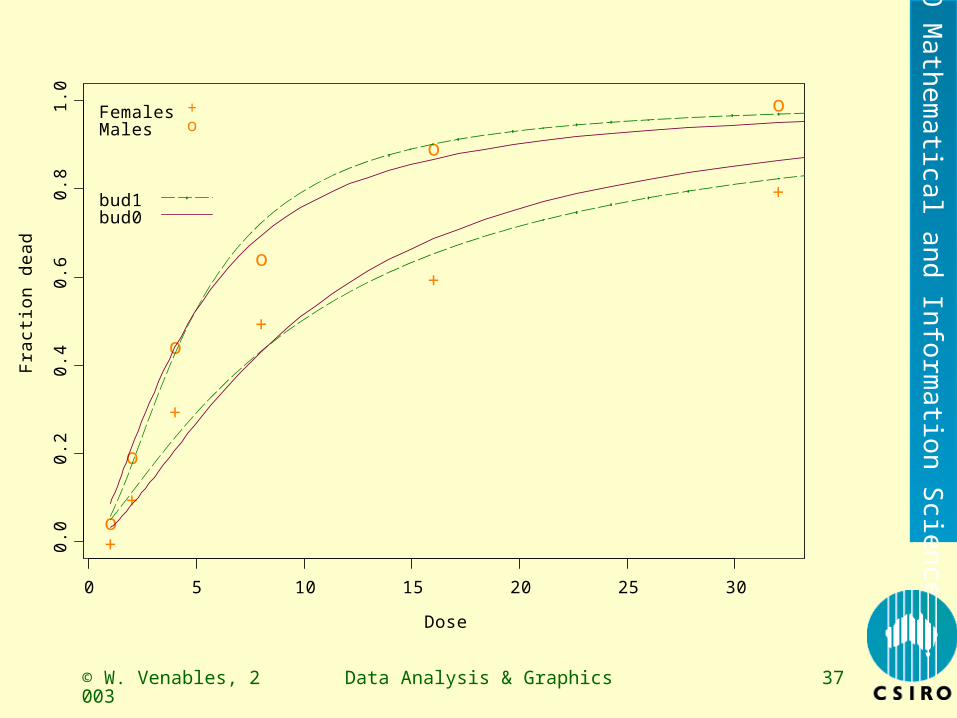
Plotting the resultsattach(Budworms)plot(2^Logdose, Dead/20, xlab = "Dose",
ylab = "Fraction dead", type = "n")text(2^Logdose, Dead/20, c("+","o")[Sex], col = 5,
cex = 1.25)newdat <- expand.grid(Logdose = seq(-0.1, 5.1, 0.1),
Sex = levels(Sex))newdat$Pr1 <- predict(bud.1, newdat, type = "response")newdat$Pr0 <- predict(bud.0, newdat, type = "response")ditch <- newdat$Logdose == 5.1 | newdat$Logdose < 0newdat[ditch, ] <- NAattach(newdat)lines(2^Logdose, Pr1, col=4, lty = 4)lines(2^Logdose, Pr0, col=3)
© W. Venables, 2003
Data Analysis & Graphics 37
CS
IRO
Math
em
atica
l an
d In
form
atio
n S
cien
ces
Dose
Fra
ctio
n d
ea
d
0 5 10 15 20 25 30
0.0
0.2
0.4
0.6
0.8
1.0
o
o
o
o
o
o
+
+
+
+
+
+
FemalesMales
+o
bud1bud0

© W. Venables, 2003
Data Analysis & Graphics 38
CS
IRO
Math
em
atica
l an
d In
form
atio
n S
cien
ces
Janka data, first re-visit
From transformations it becomes clear that
– A square-root makes the regression straight-line,
– A log is needed to make the variance constant.
One way to accommodate both is to use a GLM with
– Square-root link, and
– Variance proportional to the square of the mean.
This is done using the quasi family which allows link and
variance functions to be separately specified.
family = quasi(link = sqrt, variance = "mu^2")

© W. Venables, 2003
Data Analysis & Graphics 39
CS
IRO
Math
em
atica
l an
d In
form
atio
n S
cien
ces
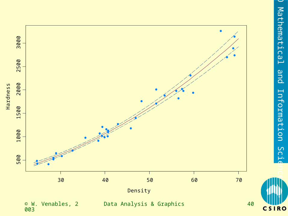
> jank.g1 <- glm(Hard ~ Dens, quasi(link = sqrt, variance = "mu^2"), janka, trace=T)
GLM linear loop 1: deviance = 0.3335 GLM linear loop 2: deviance = 0.3288 GLM linear loop 3: deviance = 0.3288 > range(janka$Dens)[1] 24.7 69.1> newdat <- data.frame(Dens = 24:70)> p1 <- predict(jank.g1, newdat, type = "response", se = T)> names(p1)[1] "fit" "se.fit" "residual.scale"[4] "df" > ul <- p1$fit + 2*p1$se.fit> ll <- p1$fit - 2*p1$se.fit> mn <- p1$fit> matplot(newdat$Dens, cbind(ll, mn, ul),
xlab = "Density", ylab = "Hardness",col = c(2,3,2), lty = c(4,1,4), type = "l")
> points(janka$Dens, janka$Hard, pch=16, col = 6)
© W. Venables, 2003
Data Analysis & Graphics 40
CS
IRO
Math
em
atica
l an
d In
form
atio
n S
cien
ces
Density
Ha
rdn
ess
30 40 50 60 70
50
01
00
01
50
02
00
02
50
03
00
0

© W. Venables, 2003
Data Analysis & Graphics 41
CS
IRO
Math
em
atica
l an
d In
form
atio
n S
cien
ces
Negative Binomial Models
• Useful class of models for count data cases where the
variance is much greater than the mean
• A Poisson model to such data will give a deviance much
greater than the residual degrees of freedom.
• Has two interpretations
– As a conditional Poisson model but with an unobserved
random effect attached to each observation
– As a "contagious distribution": the observations are
sums of a Poisson number of "clumps" with each
clump logarithmically distributed.

© W. Venables, 2003
Data Analysis & Graphics 42
CS
IRO
Math
em
atica
l an
d In
form
atio
n S
cien
ces
The quine data
• Numbers of days absent from school per pupil in a year in a rural NSW town.
• Classified by four factors:> lapply(quine, levels)$Eth:[1] "A" "N"$Sex:[1] "F" "M"$Age:[1] "F0" "F1" "F2" "F3"$Lrn:[1] "AL" "SL"$Days:NULL

© W. Venables, 2003
Data Analysis & Graphics 43
CS
IRO
Math
em
atica
l an
d In
form
atio
n S
cien
ces
First consider a Poisson "full" model"> quine.1 <- glm(Days ~ Eth*Sex*Age*Lrn, poisson, quine,
trace = T)…GLM linear loop 4: deviance = 1173.9 > quine.1$df[1] 118
Overdispersion. Now a NB model with the same mean structure (and default log link):> quine.n1 <- glm.nb(Days ~ Eth*Sex*Age*Lrn, quine,
trace=T)…Theta( 1 ) = 1.92836 , 2(Ls - Lm) = 167.453 > dropterm(quine.n1, test = "Chisq")Single term deletions
Model:Days ~ Eth * Sex * Age * Lrn Df AIC LRT Pr(Chi) <none> 1095.3 Eth:Sex:Age:Lrn 2 1092.7 1.4038 0.49563

© W. Venables, 2003
Data Analysis & Graphics 44
CS
IRO
Math
em
atica
l an
d In
form
atio
n S
cien
ces
Manual model building
• Is always risky!• Is nearly always revealing.
> quine.up <- glm.nb(Days ~ Eth*Sex*Age*Lrn, quine)> quine.m <- glm.nb(Days ~ Eth + Sex + Age + Lrn,
quine)> dropterm(quine.m, test="Chisq")Single term deletions
Model:Days ~ Eth + Sex + Age + Lrn Df AIC LRT Pr(Chi) <none> 1107.2 Eth 1 1117.7 12.524 0.00040 Sex 1 1105.4 0.250 0.61728 Age 3 1112.7 11.524 0.00921 Lrn 1 1107.7 2.502 0.11372

© W. Venables, 2003
Data Analysis & Graphics 45
CS
IRO
Math
em
atica
l an
d In
form
atio
n S
cien
ces
> addterm(quine.m, quine.up, test = "Chisq")
Single term additions
Model:
Days ~ Eth + Sex + Age + Lrn
Df AIC LRT Pr(Chi)
<none> 1107.2
Eth:Sex 1 1108.3 0.881 0.34784
Eth:Age 3 1102.7 10.463 0.01501
Sex:Age 3 1100.4 12.801 0.00509
Eth:Lrn 1 1106.1 3.029 0.08180
Sex:Lrn 1 1109.0 0.115 0.73499
Age:Lrn 2 1110.0 1.161 0.55972
> quine.m <- update(quine.m, .~.+Sex:Age)
> addterm(quine.m, quine.up, test = "Chisq")

© W. Venables, 2003
Data Analysis & Graphics 46
CS
IRO
Math
em
atica
l an
d In
form
atio
n S
cien
ces
Single term additions
Model:Days ~ Eth + Sex + Age + Lrn + Sex:Age Df AIC LRT Pr(Chi) <none> 1100.4 Eth:Sex 1 1101.1 1.216 0.27010Eth:Age 3 1094.7 11.664 0.00863Eth:Lrn 1 1099.7 2.686 0.10123Sex:Lrn 1 1100.9 1.431 0.23167Age:Lrn 2 1100.3 4.074 0.13043> quine.m <- update(quine.m, .~.+Eth:Age)> addterm(quine.m, quine.up, test = "Chisq")Single term additions
Model:Days ~ Eth + Sex + Age + Lrn + Sex:Age + Eth:Age Df AIC LRT Pr(Chi) <none> 1094.7 Eth:Sex 1 1095.4 1.2393 0.26560Eth:Lrn 1 1096.7 0.0004 0.98479Sex:Lrn 1 1094.7 1.9656 0.16092Age:Lrn 2 1094.1 4.6230 0.09911

© W. Venables, 2003
Data Analysis & Graphics 47
CS
IRO
Math
em
atica
l an
d In
form
atio
n S
cien
ces
> dropterm(quine.m, test = "Chisq")
Single term deletions
Model:
Days ~ Eth + Sex + Age + Lrn + Sex:Age + Eth:Age
Df AIC LRT Pr(Chi)
<none> 1094.7
Lrn 1 1097.9 5.166 0.023028
Sex:Age 3 1102.7 14.002 0.002902
Eth:Age 3 1100.4 11.664 0.008628
The final model (from this approach) can be written in the form
Days ~ Lrn + Age/(Eth + Sex)
suggesting that Eth and Sex have proportional effects nested within Age, and Lrn has the same proportional effect on all means independent of Age, Sex and Eth.

© W. Venables, 2003
Data Analysis & Graphics 48
CS
IRO
Math
em
atica
l an
d In
form
atio
n S
cien
ces
Generalized Additive Models: Introduction
• Strongly assumes that predictors have been chosen that are unlikely to have interactions between them.
• Weakly assumes a form for the main effect for each term!
• Estimation is done using penalized maximum likelihood where the penalty term uses a measure of roughness of the main effect forms. The tuning constant is chosen automatically by cross-validation.
• Any glm form is possible, but two additional functions, s(x, …) and lo(x,…) may be included, but only additively.
• For many models, spline models can do nearly as well!
© W. Venables, 2003
Data Analysis & Graphics 49
CS
IRO
Math
em
atica
l an
d In
form
atio
n S
cien
ces
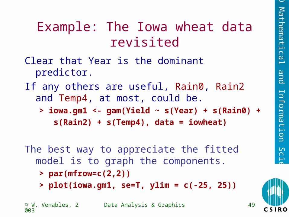
Example: The Iowa wheat data revisited
Clear that Year is the dominant predictor.If any others are useful, Rain0, Rain2 and Temp4,
at most, could be.> iowa.gm1 <- gam(Yield ~ s(Year) + s(Rain0) +
s(Rain2) + s(Temp4), data = iowheat)
The best way to appreciate the fitted model is to graph the components.> par(mfrow=c(2,2))
> plot(iowa.gm1, se=T, ylim = c(-25, 25))

© W. Venables, 2003
Data Analysis & Graphics 50
CS
IRO
Math
em
atica
l an
d In
form
atio
n S
cien
ces

© W. Venables, 2003
Data Analysis & Graphics 51
CS
IRO
Math
em
atica
l an
d In
form
atio
n S
cien
ces
Comparison with simpler models
> Iowa.fakeGAM <- lm(Yield ~ ns(Year, 3) + ns(Rain0, 3) + ns(Rain2, 3) + ns(Temp4, 3), iowheat)
> Iowa.fakePol <- lm(Yield ~ poly(Year, 3) + poly(Rain0, 3) + poly(Rain2, 3) + poly(Temp4, 3), iowheat)
> par(oma = c(0,0,4,0))
> plot.gam(Iowa.fakeGAM, se=T, ylim = c(-25, 25))> mtext("Additive components of a simple spline model",
outer = T, cex = 2)
> plot.gam(Iowa.fakePol, se=T, ylim = c(-25, 25))> mtext("Additive components of a cubic polynomial
model", outer = T, cex = 2)

© W. Venables, 2003
Data Analysis & Graphics 52
CS
IRO
Math
em
atica
l an
d In
form
atio
n S
cien
ces

© W. Venables, 2003
Data Analysis & Graphics 53
CS
IRO
Math
em
atica
l an
d In
form
atio
n S
cien
ces

© W. Venables, 2003
Data Analysis & Graphics 54
CS
IRO
Math
em
atica
l an
d In
form
atio
n S
cien
ces
GLMs with Random Effects• This is still a controversial area (Nelder, Goldstein, Diggle, …)
• Practice is not waiting for theory!
• Breslow & Clayton two procedures: "penalized quasi-
likelihood" and "marginal quasi-likelihood (PQL & MQL)
• MQL is rather like estimating equations; PQL is much closer
to the spirit of random effects.
• glmmPQL is part of the MASS library and implements PQL
using the B&C algorithm. Should be used carefully, though
for most realistic data sets the method is probably safe
enough.

© W. Venables, 2003
Data Analysis & Graphics 55
CS
IRO
Math
em
atica
l an
d In
form
atio
n S
cien
ces
A test: the quine data with Poisson PQL
• The negative binomial model has an interpretation as a poisson model with a single random effect for each observation.
• If the random effect has a 'log of gamma' distribution the exact likelihood can be computed and maximized (glm.nb).
• If the random effect has a normal distribution the integration is not feasable and approximate methods of estimation are needed.
• The two models, in principle, should be very similar. Are they in practice?

© W. Venables, 2003
Data Analysis & Graphics 56
CS
IRO
Math
em
atica
l an
d In
form
atio
n S
cien
ces
First, re-fit the preferred NB model:> quine.nb <- glm.nb(Days ~ Lrn +
Age/(Eth + Sex), quine)
Now make a local copy of quine, add the additional component and fit the (large) random effects model:
> quine <- quine
> quine$Child <- factor(1:nrow(quine))
> library(MASS, first = T)
> quine.re <- glmmPQL(Days ~ Lrn +
Age/(Eth + Sex), family = poisson(link = log), data = quine, random = ~1 | Child, maxit = 20)
iteration 1
iteration 2
...
iteration 10

© W. Venables, 2003
Data Analysis & Graphics 57
CS
IRO
Math
em
atica
l an
d In
form
atio
n S
cien
ces
How similar are the coefficients (and SE)?
> b.nb <- coef(quine.nb)
> b.re <- fixed.effects(quine.re)
> rbind(NB = b.nb, RE = b.re)
(Intercept) Lrn AgeF1 AgeF2 AgeF3
NB 2.8651 0.43464 -0.26946 -0.035837 -0.20542
RE 2.6889 0.36301 -0.24835 -0.058735 -0.30111
AgeF0Eth AgeF1Eth AgeF2Eth AgeF3Eth AgeF0Sex AgeF1Sex
NB 0.012582 -0.74511 -1.2082 -0.040114 -0.54904 -0.52050
RE -0.030215 -0.76261 -1.1759 -0.079303 -0.61111 -0.44163
AgeF2Sex AgeF3Sex
NB 0.66164 0.66438
RE 0.66571 0.77235

© W. Venables, 2003
Data Analysis & Graphics 58
CS
IRO
Math
em
atica
l an
d In
form
atio
n S
cien
ces
> se.re <- sqrt(diag(quine.re$varFix))
> se.nb <- sqrt(diag(vcov(quine.nb)))
> rbind(se.re, se.nb)
[,1] [,2] [,3] [,4] [,5] [,6]
se.re 0.28100 0.16063 0.33832 0.36867 0.35762 0.29025
se.nb 0.31464 0.18377 0.37982 0.41264 0.40101 0.32811
[,7] [,8] [,9] [,10] [,11] [,12]
se.re 0.22531 0.23852 0.26244 0.30130 0.24281 0.25532
se.nb 0.25926 0.26941 0.29324 0.33882 0.28577 0.28857
[,13]
se.re 0.26538
se.nb 0.29553
> plot(b.nb/se.nb, b.re/se.re)
> abline(0, 1, col = 3, lty = 4)

© W. Venables, 2003
Data Analysis & Graphics 59
CS
IRO
Math
em
atica
l an
d In
form
atio
n S
cien
ces
GLMM coefficientsvs Negative Binomial(both standardized).

© W. Venables, 2003
Data Analysis & Graphics 60
CS
IRO
Math
em
atica
l an
d In
form
atio
n S
cien
ces
Comparing predictions
• The negative binomial fitted values should be comparable with the "level 0" predictions from the GLMM, i.e. fixed effects only.
• The predict generic function predicts on the link scale. For the GLMM we need a correction to go from the log scale to the direct scale (cf. lognormal distribution).
• An approximate correction (on the log scale) is σ²/2 where σ² is the variance of the random effects (or BLUPs).

© W. Venables, 2003
Data Analysis & Graphics 61
CS
IRO
Math
em
atica
l an
d In
form
atio
n S
cien
ces
> fv.nb <- fitted(quine.nb)
> fv.re <- exp(predict(quine.re, level = 0) + var(random.effects(quine.re))/2)
> plot(fv.re, fv.nb)
> plot(fv.nb, fv.re)
> abline(0, 1, col = 5, lty = 4)
GLMM vs NBpredictions onthe original scale.

© W. Venables, 2003
Data Analysis & Graphics 62
CS
IRO
Math
em
atica
l an
d In
form
atio
n S
cien
ces
Non-linear regression
• Generalization of linear regression.
• Normality and equal variance retained, linearity of parameters relaxed.
• Generally comes from a fairly secure theory; not often appropriate for empirical work
• Estimation is still by least squares (= maximum likelihood), but the sum of squares surface is not necessarily quadratic.
• Theory is approximate and relies on SSQ surface being nearly quadratic in a region around the minimum.

© W. Venables, 2003
Data Analysis & Graphics 63
CS
IRO
Math
em
atica
l an
d In
form
atio
n S
cien
ces
The Stormer Viscometer DataSUMMARY:The stormer viscometer measures the viscosity of a fluid by measuring the time taken for an inner cylinder in the mechanism to perform a fixed number of revolutions in response to an actuating weight. The viscometer is calibrated by measuring the time taken with varying weights while the mechanism is suspended in fluids of accurately known viscosity. The data comes from such a calibration, and theoretical considerations suggest a non-linear relationship between time, weight and viscosity, of the form
where β1 and β2 are unknown parameters to be estimated, and E is error.
DATA DESCRIPTION:
The data frame contains the following components:
ARGUMENTS:
Viscosity Viscosity of fluid
Wt Actuating weight
Time Time taken
SOURCE:
E. J. Williams (1959) Regression Analysis. Wiley.
1
2
VT
W
© W. Venables, 2003
Data Analysis & Graphics 64
CS
IRO
Math
em
atica
l an
d In
form
atio
n S
cien
ces
A simple example
• Stormer viscometer data (data frame stormer in MASS).
> names(stormer)
[1] "Viscosity" "Wt" "Time"
• Model:
T = β V/(W – θ) + error
• Ignoring error and re-arranging gives:WT ≃ β V + θ T
• Fit this relationship with ordinary least squares to get initial values for β and θ.

© W. Venables, 2003
Data Analysis & Graphics 65
CS
IRO
Math
em
atica
l an
d In
form
atio
n S
cien
ces
Fitting the model
Is very easy for this example…> b <- coef(lm(Wt*Time ~ Viscosity + Time - 1,
stormer))> names(b) <- c("beta", "theta")> b beta theta 28.876 2.8437> storm.1 <-
nls(Time ~ beta*Viscosity/(Wt - theta), stormer, start=b,
trace=T)885.365 : 28.8755 2.84373 825.110 : 29.3935 2.23328 825.051 : 29.4013 2.21823

© W. Venables, 2003
Data Analysis & Graphics 66
CS
IRO
Math
em
atica
l an
d In
form
atio
n S
cien
ces
Looking at the results
> summary(storm.1)Formula: Time ~ (beta * Viscosity)/(Wt - theta)
Parameters: Value Std. Error t value beta 29.4013 0.91553 32.1138theta 2.2182 0.66552 3.3331
Residual standard error: 6.26803 on 21 degrees of freedom
Correlation of Parameter Estimates: beta theta -0.92

© W. Venables, 2003
Data Analysis & Graphics 67
CS
IRO
Math
em
atica
l an
d In
form
atio
n S
cien
ces
Self-starting models
Allows the starting procedure to be encoded into the model function. (Somewhat arcane but very powerful)
> library(nls) # R only> library(MASS)> data(stormer) # R only> storm.init <- function(mCall, data, LHS) { v <- eval(mCall[["V"]], data) w <- eval(mCall[["W"]], data) t <- eval(LHS, data) b <- lsfit(cbind(v, t), t * w, int = F)$coef names(b) <- mCall[c("b", "t")] b }> NLSstormer <- selfStart( ~ b*V/(W-t), storm.init,
c("b","t"))> args(NLSstormer)function(V, W, b, t)NULL …

© W. Venables, 2003
Data Analysis & Graphics 68
CS
IRO
Math
em
atica
l an
d In
form
atio
n S
cien
ces
> tst <- nls(Time ~ NLSstormer(Viscosity, Wt, beta,theta), stormer, trace = T)
885.365 : 28.8755 2.84373 825.110 : 29.3935 2.23328 825.051 : 29.4013 2.21823
Bootstrapping is NBD:
> tst$call$trace <- NULL> B <- matrix(NA, 500, 2)> r <- scale(resid(tst), scale = F) # mean correct> f <- fitted(tst)> for(i in 1:500) {
v <- f + sample(r, rep = T) B[i, ] <- try(coef(update(tst, v ~ .))) # guard!}
> cbind(Coef = colMeans(B), SD = colStdevs(B)) Coef SD [1,] 29.4215 0.64390[2,] 2.2204 0.46051

© W. Venables, 2003
Data Analysis & Graphics 69
CS
IRO
Math
em
atica
l an
d In
form
atio
n S
cien
ces
NLS example: the muscle data
• Old data from an experiment on muscle contraction in experimental animals.
• Variables:
– Strip: identifier of muscle (animal)
– Conc: CaCl concentrations used to soak the section
– Length: resulting length of muscle section for each concentration
• Model: L = α + β exp(-C/ θ) + error
where α and β may vary with the animal but θ is constant.
• Note that α and β are (very many) linear parameters. We use
this strongly

© W. Venables, 2003
Data Analysis & Graphics 70
CS
IRO
Math
em
atica
l an
d In
form
atio
n S
cien
ces
First model: fixed parameters• Since there are 21 animals with separate alpha's and
beta's for each the number of parameters is 21+21+1=43, from 61 observations!
• Use the plinear algorithm since all parameters are linear bar one.> X <- model.matrix(~ Strip – 1, muscle)
> musc.1 <- nls(Length ~ cbind(X, X*exp(-Conc/th)),
muscle, start = list(th = 1), algorithm = "plinear",
trace = T)
....
> b <- coef(musc.1)
> b
th .lin1 .lin2 .lin3 .lin4 .lin5 .lin6 .lin7
0.79689 23.454 28.302 30.801 25.921 23.2 20.12 33.595.......lin39 .lin40 .lin41 .lin42
-15.897 -28.97 -36.918 -26.508

© W. Venables, 2003
Data Analysis & Graphics 71
CS
IRO
Math
em
atica
l an
d In
form
atio
n S
cien
ces
Conventional fitting algorithm
• Parameters in non-linear regression may be indexed:> th <- b[1]
> a <- b[2:22]
> b <- b[23:43]
> musc.2 <- nls(Length ~ a[Strip] +
b[Strip)*exp(-Conc/th),
muscle, start = list(a = a, b = b, th = th),
trace = T)
......
• Converges in one step, now.• Note that with indexed parameters, the starting values
must be given in a list (with names).

© W. Venables, 2003
Data Analysis & Graphics 72
CS
IRO
Math
em
atica
l an
d In
form
atio
n S
cien
ces
Plotting the result
> range(muscle$Conc)
[1] 0.25 4.00
> newdat <- expand.grid(
Strip = levels(muscle$Strip),
Conc = seq(0.25, 4, 0.05))
> dim(newdat)
[1] 1596 2
> names(newdat)
[1] "Strip" "Conc"
> newdat$Length <- predict(musc.2, newdat)

© W. Venables, 2003
Data Analysis & Graphics 73
CS
IRO
Math
em
atica
l an
d In
form
atio
n S
cien
ces
The actual plot
Trellis comes to the rescue:
> xyplot(Length ~ Conc | Strip, muscle, subscripts = T,
panel = function(x, y, subscripts, ...) {
panel.xyplot(x, y, ...)
ws <- as(muscle$Strip[subscripts[1]], "character")
wf <- which(newdat$Strip == ws)
xx <- newdat$Conc[wf]
yy <- newdat$Length[wf]
lines(xx, yy, col = 3)
}, ylim = range(newdat$Length, muscle$Length),
as.table = T)

© W. Venables, 2003
Data Analysis & Graphics 74
CS
IRO
Math
em
atica
l an
d In
form
atio
n S
cien
ces

© W. Venables, 2003
Data Analysis & Graphics 75
CS
IRO
Math
em
atica
l an
d In
form
atio
n S
cien
ces
A Random Effects version
• Random effects models allow the parametric dimension to be more easily controlled.
• We assume α and β are now random over animals
> musc.re <- nlme(Length ~ a + b*exp(-Conc/th),
fixed = a+b+th~1, random = a+b~1|Strip,
data = muscle, start =
c(a=mean(a), b=mean(b), th=th))
• The vectors a, b and th come from the previous fit; no need to supply initial values for the random effects, (though you may).

© W. Venables, 2003
Data Analysis & Graphics 76
CS
IRO
Math
em
atica
l an
d In
form
atio
n S
cien
ces
A composite plot
> newdat$L2 <- predict(musc.re, newdat)
> xyplot(Length ~ Conc | Strip, muscle, subscripts = T, panel =
function(x, y, subscripts, ...) {
panel.xyplot(x, y, ...)
ws <- as(muscle$Strip[subscripts[1]], "character")
wf <- which(newdat$Strip == ws)
xx <- newdat$Conc[wf]
yy <- newdat$Length[wf]
lines(xx, yy, col = 3)
yy <- newdat$L2[wf]
lines(xx, yy, lty=4, col=4)
}, ylim = range(newdat$Length, muscle$Length), as.table = T)

© W. Venables, 2003
Data Analysis & Graphics 77
CS
IRO
Math
em
atica
l an
d In
form
atio
n S
cien
ces

© W. Venables, 2003
Data Analysis & Graphics 78
CS
IRO
Math
em
atica
l an
d In
form
atio
n S
cien
ces
Tree based methods - an introduction
V&R, Ch. 9 (formerly 10).
• A decision tree is a sequence of binary rules leading to one of a number of terminal nodes, each associated with some decision.
• A classification tree is a decision tree that attempts to reproduce a given classification as economically as possible.
• A variable is selected and the population is divided into two at a selected breakpoint of that variable.
• Each half is then independently subdivided further on the same principle, thus recursively forming a binary tree structure.
• Each node is associated with a probability forecast for membership in each class (hopefully as specific as possible).

© W. Venables, 2003
Data Analysis & Graphics 79
CS
IRO
Math
em
atica
l an
d In
form
atio
n S
cien
cesA < 3
B < 2
A < 1C < 10B < 1
D = fgFemale
Male
FemaleFemale
MaleMale
Female
A generic classification tree with 7 terminal nodes.

© W. Venables, 2003
Data Analysis & Graphics 80
CS
IRO
Math
em
atica
l an
d In
form
atio
n S
cien
ces
Trees, more preliminaries
– The faithfulness of any classification tree is measured by a deviance measure, D(T), which takes its miminum value at zero if every member of the training sample is uniquely and correctly classified.
– The size of a tree is the number of terminal nodes.– A cost-complexity measure of a tree is the deviance
penalized by a multiple of the size:
D(T) = D(T) + α size(T)
where α is a tuning constant. This is eventually minimized.
– Low values of α for this measure imply that accuracy of prediction (in the training sample) is more important than simplicity.
– High values of α rate simplicity relatively more highly than predictive accuracy.

© W. Venables, 2003
Data Analysis & Graphics 81
CS
IRO
Math
em
atica
l an
d In
form
atio
n S
cien
ces
Regression trees• Suppose Y has a distribution with mean depending on several
determining variables, not necessarily continuous.
• A regression tree is a decision tree that partitions the determining variable space into non-overlapping prediction regions.
• Within each prediction region the response variable Y is predictied by a constant.
• The deviance in this case is exactly the same as for regression: the residual sum of squares.
– With enough regions (nodes) the training sample can clearly be reproduced exactly, but predictions will be inaccurate.
– With too few nodes predictions may be seriously biased.
• How many nodes should we use? This is the key question for all of tree modelling (equivalent to setting the tuning constant).

© W. Venables, 2003
Data Analysis & Graphics 82
CS
IRO
Math
em
atica
l an
d In
form
atio
n S
cien
ces
Some S tree model facilities
ftr <- tree(formula, data = dataFrame, ...)rtr <- rpart(formula, data = dataFrame, ...)
implements an algorithm to produce a binary tree (regression or classification) and returns a tree object.
The formula is of the simple formR ~ X1 +X2 + …
where R is the target variable and X1, X2,... are
the determining variables. if R is a factor the result is a classification tree, if R is numeric the result is a regression tree.

© W. Venables, 2003
Data Analysis & Graphics 83
CS
IRO
Math
em
atica
l an
d In
form
atio
n S
cien
ces
tree or rpart?
• In S-PLUS there is a native tree library that V&R have some reservations about. It is useful, though.
• rpart is a library written by Beth Atkinson and Terry Therneau of the Mayo Clinic, Rochester, NY. It is much closer to the spirit of the original CART algorithm of Breiman, et al. It is now supplied with both S-PLUS and R.
• In R, there is a tree library that is an S-PLUS look-alike, but we think better in some respects.
• rpart is the more flexible and allows various splitting criteria and different model bases (survival trees, for example).
• rpart is probably the better package, but tree is acceptable and some things such as cross-validation are easier with tree.
• In this discussion we (nevertheless) largely use tree!

© W. Venables, 2003
Data Analysis & Graphics 84
CS
IRO
Math
em
atica
l an
d In
form
atio
n S
cien
ces
Some other arguments to tree
There are a number of other optional important arguments, for example:
na.action = na.omit
indicates that cases with missing observations on some requried variable are to be omitted.
By default the algorithm terminates the splitting when the group is either homogeneous or of size 5 or less. Occasionally it is useful to remove or tighten this restriction, and so
minsize = k
specifics that the groups may be as small as k.

© W. Venables, 2003
Data Analysis & Graphics 85
CS
IRO
Math
em
atica
l an
d In
form
atio
n S
cien
ces
Displaying and interrogating a tree
> plot(ftr)
> text(ftr)
will give a graphical representation of the tree, as well as text to indicate how the tree has been constructed.
The assignment> nodes <- identify(ftr)
allows interactive identification of the cases in each node.Clicking on any node produces a list of row labels in the
working window.Clicking on the right button terminates the interactive action.
The result is an S list giving the contents (as character string vector components) of the nodes selected.

© W. Venables, 2003
Data Analysis & Graphics 86
CS
IRO
Math
em
atica
l an
d In
form
atio
n S
cien
ces
An simplistic example: The Janka data
Consider predicting trees by, well, trees!
> jank.t1 <- tree(Hard ~ Dens, janka)> jank.t1node), split, n, deviance, yval * denotes terminal node 1) root 36 22000000 1500 2) Dens<47.55 21 1900000 890 4) Dens<34.15 8 73000 540 * 5) Dens>34.15 13 220000 1100 * 3) Dens>47.55 15 3900000 2300 6) Dens<62.9 10 250000 1900 12) Dens<56.25 5 69000 1900 * 13) Dens>56.25 5 130000 2000 * 7) Dens>62.9 5 240000 2900 *
The tree has 5 terminal nodes. We can take two views of the model that complement each other.

© W. Venables, 2003
Data Analysis & Graphics 87
CS
IRO
Math
em
atica
l an
d In
form
atio
n S
cien
ces
> plot(jank.t1, lwd = 2, col = 6)> text(jank.t1, cex = 1.25, col = 5)

© W. Venables, 2003
Data Analysis & Graphics 88
CS
IRO
Math
em
atica
l an
d In
form
atio
n S
cien
ces
> partition.tree(jank.t1, xlim = c(24, 70))> attach(janka)> points(Dens, Hard, col = 5, cex = 1.25)> segments(Dens, Hard, Dens, predict(jank.t1),
col = 6, lty = 4)

© W. Venables, 2003
Data Analysis & Graphics 89
CS
IRO
Math
em
atica
l an
d In
form
atio
n S
cien
ces
A classification tree: Bagging
• Survey data (data frame survey from the MASS library).
> ?survey
> names(survey)
[1] "Sex" "Wr.Hnd" "NW.Hnd" "W.Hnd" "Fold" "Pulse"
[7] "Clap" "Exer" "Smoke" "Height" "M.I" "Age"
• We consider predicting Sex from the other variables.
• Remove cases with missing values
• Split data set into "Training" and "Test" sets
• Build model in training set, test in test.
• Look at simple "bagging" to improve stability and predictions

© W. Venables, 2003
Data Analysis & Graphics 90
CS
IRO
Math
em
atica
l an
d In
form
atio
n S
cien
ces
Preliminary manipulations
We start with a bit of data cleaning.> dim(survey)
[1] 237 12
> count.nas <- function(x) sum(is.na(x))
> sapply(survey, count.nas)
Sex Wr.Hnd NW.Hnd W.Hnd Fold Pulse Clap Exer Smoke Height
1 1 1 1 0 45 1 0 1 28
M.I Age
28 0
> Srvy <- na.omit(survey)
> dim(Srvy)
[1] 168 12

© W. Venables, 2003
Data Analysis & Graphics 91
CS
IRO
Math
em
atica
l an
d In
form
atio
n S
cien
ces
Initial fitting to all data and display of the result
> surv.t1 <- tree(Sex ~ .,Srvy)
> plot(surv.t1)> text(surv.t1, col = 5)

© W. Venables, 2003
Data Analysis & Graphics 92
CS
IRO
Math
em
atica
l an
d In
form
atio
n S
cien
ces
Cross-validation
A technique for using internal evidence to guage the size of tree warranted by the data.
Random sections are omitted and the remainder used to construct a tree. The ommitted section is then predicted from the remainder and various criteria (deviance, error rate) used to assess the efficacy.
> obj <- cv.tree(tree.obj, FUN=functn, ...)
> plot(obj)
Currently functn must be either prune.tree or shrink.tree (the default). It determines the protocol by which the sequence of trees tested is generated. The MASS library also has prune.misclass for classification trees, only.

© W. Venables, 2003
Data Analysis & Graphics 93
CS
IRO
Math
em
atica
l an
d In
form
atio
n S
cien
ces
Cross-validation as a guide to pruning:
> surv.t1cv <- cv.tree(surv.t1, FUN = prune.misclass)
> plot(surv.t1cv)

© W. Venables, 2003
Data Analysis & Graphics 94
CS
IRO
Math
em
atica
l an
d In
form
atio
n S
cien
ces
Pruning> surv.t2 <- prune.tree(surv.t1, best = 6)> plot(surv.t2)> text(surv.t2, col = 5)

© W. Venables, 2003
Data Analysis & Graphics 95
CS
IRO
Math
em
atica
l an
d In
form
atio
n S
cien
ces
rpart counterpart
> rp1 <- rpart(Sex ~ ., Srvy,
minsplit = 10)
> plot(rp1)
> text(rp1)
> plotcp(rp1)
See next slide. This suggests a very small tree – two nodes. (Some repeat tests might be necessary.)
> rp2 <- prune(rp1, cp = 0.29)
> plot(rp2)
> text(rp2)

© W. Venables, 2003
Data Analysis & Graphics 96
CS
IRO
Math
em
atica
l an
d In
form
atio
n S
cien
ces
rpart tree with minsplit = 10
Internal cross-validation and the 'one se' rule

© W. Venables, 2003
Data Analysis & Graphics 97
CS
IRO
Math
em
atica
l an
d In
form
atio
n S
cien
ces
Confusion matrices
• Now to check the effectiveness of the pruned tree on the training sample.
• Should be pretty good!
> table(predict(surv.t2, type = "class"),
Srvy$Sex)
Female Male
Female 79 11
Male 5 73
• Next step: build on a training set, test on a test.

© W. Venables, 2003
Data Analysis & Graphics 98
CS
IRO
Math
em
atica
l an
d In
form
atio
n S
cien
ces
First build the model.> w <- sample(nrow(Srvy), nrow(Srvy)/2)> Surv0 <- Srvy[w, ]> Surv1 <- Srvy[-w, ]> surv.t3 <- tree(Sex ~ ., Surv0)
Check on training set:> table(predict(surv.t3, type="class"),
Surv0$Sex) Female Male Female 42 2 Male 3 37
Test on test set:> table(predict(surv.t3, Surv1, type="class"), Surv1$Sex)
Female Male Female 34 6 Male 5 39

© W. Venables, 2003
Data Analysis & Graphics 99
CS
IRO
Math
em
atica
l an
d In
form
atio
n S
cien
ces
Now build an over-fitted model on the training set and check its performance:> surv.t3 <- tree(Sex ~ ., Surv0, minsize = 4)
> table(predict(surv.t3, type="class"), Surv0$Sex)
Female Male
Female 44 1
Male 1 38
Far too good! How does it look on the test set?> table(predict(surv.t3, Surv1, type="class"),
Surv1$Sex)
Female Male
Female 31 9
Male 8 36

© W. Venables, 2003
Data Analysis & Graphics 100
CS
IRO
Math
em
atica
l an
d In
form
atio
n S
cien
ces
Bagging requires fitting the same model a sequence of 'bootstrapped data frames'. It is convenient to have a function to do it.> jig <- function(dataFrame)
dataFrame[sample(nrow(dataFrame), rep = T), ]
Now for the bagging itself
> bag <- list()> for(i in 1:100)
bag[[i]] <- update(surv.t3, data = jig(Surv0))
Next find the sequence of predictions for each model using the test set. It is convenient to have the result as characters.
> bag.pred <- lapply(bag, predict, newdata = Surv1, type = "class")
> bag.pred <- lapply(bag.pred, as.character)

© W. Venables, 2003
Data Analysis & Graphics 101
CS
IRO
Math
em
atica
l an
d In
form
atio
n S
cien
ces
Finding the winnerUsing a single call to table(), find the frequency of each
prediction for each row of Surv1:
> tab <- table(rep(1:nrow(Surv1), 100), unlist(bag.pred))
Now find the maxima, avoiding any "one at a time" method.
> maxv <- tab[,1]> maxp <- rep(1, nrow(tab))> for(j in 2:ncol(tab)) {
v <- maxv < tab[,j] if(any(v)) { maxv[v] <- tab[v, j] maxp[v] <- j }
}> table(levels(Surv1$Sex)[maxp], Surv1$Sex) Female Male Female 36 7 Male 3 38Now 10 rather than 17 misclassifications.

© W. Venables, 2003
Data Analysis & Graphics 102
CS
IRO
Math
em
atica
l an
d In
form
atio
n S
cien
ces
Tree models: some pros and cons
• Tree based models are easy to appreciate and discuss. The important variables stand out. Non-additive and non-linear behaviour is automatically captured.
• Mixed factor and numeric variables are simply accommodated.
• The scale problem for the response is no worse than it is in the regression case.
• Linear dependence in the predictors is irrelevant, as are monotone transformations of predictors.
• Experience with the technique is still in its infancy. The theoretical basis is still very incomplete.
• Strongly coordinate dependent in the predictors.• Unstable in general.• Non-uniqueness. Two practitioners will often end up with
different trees. This is not important if inference is not envisaged.

© W. Venables, 2003
Data Analysis & Graphics 103
CS
IRO
Math
em
atica
l an
d In
form
atio
n S
cien
ces
An Overview of some Multivariate Analysis Facilities
• Multivariate Linear Models and other classical techniques– manova, summary.manova– lda, qda (in MASS)– princomp, cancor, biplot, factanal, (in mva on
R)• Ordination and classification (clustering)
– dist, hclust, cmdscale, plclust, kmeans (in mva on R),
– isoMDS, sammon, corresp, biplot.corresp (in MASS)
– agnes, clara, daisy, diana, fanny, mona, pam (in cluster on R)
– cca, rda, decorana, decostand, vegdist (in vegan, only in R)

© W. Venables, 2003
Data Analysis & Graphics 104
CS
IRO
Math
em
atica
l an
d In
form
atio
n S
cien
ces
Distances, Ordination and Clustering
• Distances:– dist – only euclidean or manhattan– daisy – only euclidean or manhattan for continuous,
handles some discrete cases as well– vegdist (in vegan, only on R) – handles Bray-Curtis
and some others• Ordination based on distances:
– cmdscale – classical metric (in mva)– isoMDS, sammon – non-metric scaling (in MASS)
• Clustering from distances:– hclust (in mva)– pam, fanny, agnes, diana (in cluster)

© W. Venables, 2003
Data Analysis & Graphics 105
CS
IRO
Math
em
atica
l an
d In
form
atio
n S
cien
ces
Distances, Ordination and Clustering, cont'd
• Ordination not based on distances:– princomp (in mva) – rather simplistic– cca, rda, decorana (in vegan); corresp (in MASS) variants on correspondence analysis
• Clustering not based on distances:– kmeans (in mva) – effectively euclidean
distances– clara (in cluster) – either euclidean or
manhattan; handles very large data sets– mona (in cluster) – binary data only. Splits
on one variable at a time (like tree models).

© W. Venables, 2003
Data Analysis & Graphics 106
CS
IRO
Math
em
atica
l an
d In
form
atio
n S
cien
ces
Silhouette plots and coefficients (cluster)
• For each object, plots a relative membership measure (with range: -1 < m < 1) of the group to which it has been assigned to the best supported alternative group
• the plot presents all objects as vertical 'bands' of 'width' m
• The 'average width' the cluster coefficient:
‣ 0.70 < m < 1.00: Good structure has been found‣ 0.50 < m < 0.70: Reasonable structure found‣ 0.25 < m < 0.50: Weak structure, requiring
confirmation‣ -1 < m < 0.25: Forget it!

© W. Venables, 2003
Data Analysis & Graphics 107
CS
IRO
Math
em
atica
l an
d In
form
atio
n S
cien
ces
Example: Epibenthic Sled data from GoC
> dim(DredgeWT)
[1] 146 1389
> range(DredgeWT)
[1] 0.00 1937.68
> ddredge <- dist.brayCurtis(log(1 + DredgeWT))
> ?agnes
> agdredge <- agnes(ddredge, method = "ward")
> plot(agdredge)
Hit <Return> to see next plot:
Hit <Return> to see next plot:
>

© W. Venables, 2003
Data Analysis & Graphics 108
CS
IRO
Math
em
atica
l an
d In
form
atio
n S
cien
ces

© W. Venables, 2003
Data Analysis & Graphics 109
CS
IRO
Math
em
atica
l an
d In
form
atio
n S
cien
ces

© W. Venables, 2003
Data Analysis & Graphics 110
CS
IRO
Math
em
atica
l an
d In
form
atio
n S
cien
ces
Geographical Identification
> dgroups <- cutree(agdredge, k = 4)> table(dgroups)dgroups 1 2 3 4 60 46 33 7 > attach(DredgeX)> library(MASS)> eqscplot(Longitude, Latitude, type="n", axes=F,
xlab="", ylab="")> points(Longitude, Latitude, pch = dgroups, col
= c("red", "yellow", "green", "blue")[dgroups])> library(Aus) # Nick Ellis> Aus(add = T, col = "brown")

© W. Venables, 2003
Data Analysis & Graphics 111
CS
IRO
Math
em
atica
l an
d In
form
atio
n S
cien
ces

© W. Venables, 2003
Data Analysis & Graphics 112
CS
IRO
Math
em
atica
l an
d In
form
atio
n S
cien
ces
Partitioning around medoids
> pdredge <- pam(ddredge, 4)
> plot(pdredge)
Hit <Return> to see next plot:
Hit <Return> to see next plot:
> library(MASS) # if need be
> attach(DredgeX) # if need be
> eqscplot(Longitude, Latitude, pch=pdredge$cluster, col = c("red", "yellow", "green", "blue")[pdredge$cluster], axes=F, xlab="", ylab="")
> library(Aus) # if need be
> Aus(add=T)

© W. Venables, 2003
Data Analysis & Graphics 113
CS
IRO
Math
em
atica
l an
d In
form
atio
n S
cien
ces

© W. Venables, 2003
Data Analysis & Graphics 114
CS
IRO
Math
em
atica
l an
d In
form
atio
n S
cien
ces

© W. Venables, 2003
Data Analysis & Graphics 115
CS
IRO
Math
em
atica
l an
d In
form
atio
n S
cien
ces