Embed Size (px)
Citation preview
September 2002
Northeast Fisheries Science Center Reference Document 02-14
35th Northeast RegionalStock Assessment Workshop
(35th SAW)
Stock AssessmentReview Committee (SARC)
Consensus Summary of Assessments
01-18 Report of the 33rd Northeast Regional Stock Assessment Workshop (33rd SAW): Stock Assessment ReviewCommittee (SARC) Consensus Summary of Assessments. [By Northeast Regional Stock Assessment WorkshopNo. 33.] December 2001.
01-19 Report of the 33rd Northeast Regional Stock Assessment Workshop (33rd SAW): Public Review Workshop.[By Northeast Regional Stock Assessment Workshop No. 33.] December 2001.
01-20 Assessment of 19 Northeast Groundfish Stocks through 2000: A Report to the New England Fishery Manage-ment Council’s Multi-Species Monitoring Committee. By Northern Demersal and Southern Demersal WorkingGroups, Northeast Regional Stock Assessment Workshop. December 2001.
02-01 Workshop on the Effects of Fishing Gear on Marine Habitats off the Northeastern United States, October 23-25, 2001, Boston, Massachusetts. By Northeast Region Essential Fish Habitat Steering Committee. February 2002.
02-02 The 2001 Assessment of the Gulf of Maine Atlantic Cod Stock. By R.K. Mayo, E.M. Thunberg, S.E. Wigley, andS.X. Cadrin. [A report of Northeast Regional Stock Assessment Workshop No. 33.] March 2002.
02-03 An Age-Structured Assessment Model for Georges Bank Winter Flounder. By J.K.T. Brodziak. [A report ofNortheast Regional Stock Assessment Workshop No. 34.] March 2002.
02-04 Re-Evaluation of Biological Reference Points for New England Groundfish. By Working Group on Re-Evalua-tion of Biological Reference Points for New England Groundfish. March 2002.
02-05 Biological Characteristics, Population Dynamics, and Current Status of Redfish, Sebastes fasciatus Storer, inthe Gulf of Maine - Georges Bank Region. By R.K. Mayo, J.K.T. Brodziak, M. Thompson, J.M. Burnett, and S.X.Cadrin. [A report of Northeast Regional Stock Assessment Workshop No. 33.] April 2002.
02-06 Report of the 34th Northeast Regional Stock Assessment Workshop (34th SAW): Stock Assessment ReviewCommittee (SARC) Consensus Summary of Assessments. [By Northeast Regional Stock Assessment WorkshopNo. 34.] April 2002.
02-07 Report of the 34th Northeast Regional Stock Assessment Workshop (34th SAW): Public Review Workshop.[By Northeast Regional Stock Assessment Workshop No. 34.] April 2002.
02-08 Description of the 2001 Oceanographic Conditions on the Northeast Continental Shelf. By M.H. Taylor, C.Bascuñán, and J.P. Manning. May 2002.
02-09 A Compilation of Reported Fish Kills in the Hudson-Raritan Estuary during 1982 through 2001. By R.N. Reid,P.S. Olsen, and J.B. Mahoney. July 2002.
02-10 Northeast Fisheries Science Center Publications, Reports, and Abstracts for Calendar Year 2001. By L. Garnerand J.A. Gibson. August 2002.
02-11 Status of the Northeast U.S. Continental Shelf Ecosystem: A Report of the Northeast Fisheries Science Center’sEcosystem Status Working Group. By J.S. Link and J.K.T. Brodziak, editors, with contributions from (listed alpha-betically) J.K.T. Brodziak, D.D. Dow, S.F. Edwards, M.C. Fabrizio, M.J. Fogarty, D. Hart, J.W. Jossi, J. Kane, K.L.Lang, C.M. Legault, J.S. Link, S.A. MacLean, D.G. Mountain, J. Olson, W.J. Overholtz, D.L. Palka, and T.D. Smith.August 2002.
02-12 Proceedings of the Fifth Meeting of the Transboundary Resources Assessment Committee (TRAC), WoodsHole, Massachusetts, February 5-8, 2002. By R.N. O’Boyle and W.J. Overholtz, TRAC co-chairmen. [A report ofTransboundary Resources Assessment Committee Meeting No. 5]. September 2002.
02-13 Report of the 35th Northeast Regional Stock Assessment Workshop (35th SAW): Public Review Workshop.[By Northeast Regional Stock Assessment Workshop No. 35.] September 2002.
Recent Issues in This Series

Northeast Fisheries Science Center Reference Document 02-14
A Report of the 35th Northeast Regional Stock Assessment Workshop
35th Northeast RegionalStock Assessment Workshop
(35th SAW)
Stock Assessment Review Committee (SARC)Consensus Summary of Assessments
U.S. DEPARTMENT OF COMMERCENational Oceanic and Atmospheric Administration
National Marine Fisheries ServiceNortheast Region
Northeast Fisheries Science CenterWoods Hole, Massachusetts
September 2002
Northeast Fisheries Science Center Reference Documents
This series is a secondary scientific series designed to assure the long-term documentation and to enablethe timely transmission of research results by Center and/or non-Center researchers, where such results bearupon the research mission of the Center (see the outside back cover for the mission statement). Thesedocuments receive internal scientific review but no technical or copy editing. The National Marine FisheriesService does not endorse any proprietary material, process, or product mentioned in these documents.
All documents issued in this series since April 2001, and several documents issued prior to that date,have been copublished in both paper and electronic versions. To access the electronic version of a documentin this series, go to http://www.nefsc.noaa.gov/nefsc/publications/series/crdlist.htm. The electronicversion will be available in PDF format to permit printing of a paper copy directly from the Internet. If youdo not have Internet access, or if a desired document is one of the pre-April 2001 documents available onlyin the paper version, you can obtain a paper copy by contacting the senior Center author of the desireddocument. Refer to the title page of the desired document for the senior Center author's name and mailingaddress. If there is no Center author, or if there is corporate (i.e., non-individualized) authorship, thencontact the Center's Woods Hole Laboratory Library (166 Water St., Woods Hole, MA 02543-1026).
This document may be cited as:
Northeast Fisheries Science Center. 2002. Report of the 35th Northeast Regional Stock Assessment Workshop (35thSAW): Stock Assessment Review Committee (SARC) consensus summary of assessments. Northeast Fish. Sci. Cent.Ref. Doc. 02-14; 259 p. Available from: National Marine Fisheries Service, 166 Water Street, Woods Hole, MA 02543-1026.
iii
TABLE OF CONTENTS
MEETING OVERVIEW . . . . . . . . . . . . . . . . . . . . . . . . . . . . . . . . . . . . . . . . . . . . . . . . . 1
OPENING . . . . . . . . . . . . . . . . . . . . . . . . . . . . . . . . . . . . . . . . . . . . . . . . . . . . . . . 2
AGENDA . . . . . . . . . . . . . . . . . . . . . . . . . . . . . . . . . . . . . . . . . . . . . . . . . . . . . . . . 3
THE PROCESS . . . . . . . . . . . . . . . . . . . . . . . . . . . . . . . . . . . . . . . . . . . . . . . . . . . 4
AGENDA AND REPORTS . . . . . . . . . . . . . . . . . . . . . . . . . . . . . . . . . . . . . . . . . . 4
A. SUMMER FLOUNDER . . . . . . . . . . . . . . . . . . . . . . . . . . . . . . . . . . . . . . . . . . . . . . 8
TERMS OF REFERENCE . . . . . . . . . . . . . . . . . . . . . . . . . . . . . . . . . . . . . . . . . . . 8
INTRODUCTION . . . . . . . . . . . . . . . . . . . . . . . . . . . . . . . . . . . . . . . . . . . . . . . . . 8
FISHERY DATA . . . . . . . . . . . . . . . . . . . . . . . . . . . . . . . . . . . . . . . . . . . . . . . . 10Commercial Fishery Landings . . . . . . . . . . . . . . . . . . . . . . . . . . . . . . . . . . 10Northeast Region Commercial Fishery Landings . . . . . . . . . . . . . . . . . . . . 10North Carolina Commercial Fishery Landings . . . . . . . . . . . . . . . . . . . . . . 11Commercial Fishery Discards . . . . . . . . . . . . . . . . . . . . . . . . . . . . . . . . . . 12Recreational Fishery Landings . . . . . . . . . . . . . . . . . . . . . . . . . . . . . . . . . 15Recreational Fishery Discards . . . . . . . . . . . . . . . . . . . . . . . . . . . . . . . . . . . 16Total Catch Composition . . . . . . . . . . . . . . . . . . . . . . . . . . . . . . . . . . . . . . 17
BIOLOGICAL DATA . . . . . . . . . . . . . . . . . . . . . . . . . . . . . . . . . . . . . . . . . . . . . 18Aging . . . . . . . . . . . . . . . . . . . . . . . . . . . . . . . . . . . . . . . . . . . . . . . . . . . . 18Maturity . . . . . . . . . . . . . . . . . . . . . . . . . . . . . . . . . . . . . . . . . . . . . . . . . . . 19
RESEARCH SURVEY ABUNDANCE AND BIOMASS INDICES . . . . . . . . . . 20NEFSC Spring . . . . . . . . . . . . . . . . . . . . . . . . . . . . . . . . . . . . . . . . . . . . . 20NEFSC Autumn . . . . . . . . . . . . . . . . . . . . . . . . . . . . . . . . . . . . . . . . . . . 21NEFSC Winter . . . . . . . . . . . . . . . . . . . . . . . . . . . . . . . . . . . . . . . . . . . . . 21Massachusetts DMF . . . . . . . . . . . . . . . . . . . . . . . . . . . . . . . . . . . . . . . . . 22
iv
Connecticut DEP . . . . . . . . . . . . . . . . . . . . . . . . . . . . . . . . . . . . . . . . . . . 22Rhode Island DFW . . . . . . . . . . . . . . . . . . . . . . . . . . . . . . . . . . . . . . . . . . 22New Jersey BMF . . . . . . . . . . . . . . . . . . . . . . . . . . . . . . . . . . . . . . . . . . . 23Delaware DFW . . . . . . . . . . . . . . . . . . . . . . . . . . . . . . . . . . . . . . . . . . . . 23Maryland DNR . . . . . . . . . . . . . . . . . . . . . . . . . . . . . . . . . . . . . . . . . . . . . 23Virginia Institute of Marine Science . . . . . . . . . . . . . . . . . . . . . . . . . . . . . . . 23North Carolina DMF . . . . . . . . . . . . . . . . . . . . . . . . . . . . . . . . . . . . . . . . 24
ESTIMATES OF MORTALITY AND STOCK SIZE . . . . . . . . . . . . . . . . . . . . . 24Natural Mortality Rate . . . . . . . . . . . . . . . . . . . . . . . . . . . . . . . . . . . . . . . . 24ASPIC Model . . . . . . . . . . . . . . . . . . . . . . . . . . . . . . . . . . . . . . . . . . . . . . 24Virtual population analysis and tuning . . . . . . . . . . . . . . . . . . . . . . . . . . . . . 25VPA estimates of fishing mortality rates . . . . . . . . . . . . . . . . . . . . . . . . . . . 26VPA estimates of stock abundance . . . . . . . . . . . . . . . . . . . . . . . . . . . . . . . 26Precision of VPA estimates . . . . . . . . . . . . . . . . . . . . . . . . . . . . . . . . . . . . 26Retrospective analysis of VPA . . . . . . . . . . . . . . . . . . . . . . . . . . . . . . . . . 27
BIOLOGICAL REFERENCE POINTS . . . . . . . . . . . . . . . . . . . . . . . . . . . . . . . . 28
PROJECTIONS . . . . . . . . . . . . . . . . . . . . . . . . . . . . . . . . . . . . . . . . . . . . . . . . . . 28
CONCLUSIONS . . . . . . . . . . . . . . . . . . . . . . . . . . . . . . . . . . . . . . . . . . . . . . . . . 29Assessment Results . . . . . . . . . . . . . . . . . . . . . . . . . . . . . . . . . . . . . . . . . . 29
SARC COMMENTS . . . . . . . . . . . . . . . . . . . . . . . . . . . . . . . . . . . . . . . . . . . . . . 30
RESEARCH RECOMMENDATIONS . . . . . . . . . . . . . . . . . . . . . . . . . . . . . . . . . 31Major sources of assessment uncertainty . . . . . . . . . . . . . . . . . . . . . . . . . . . 32
LITERATURE CITED . . . . . . . . . . . . . . . . . . . . . . . . . . . . . . . . . . . . . . . . . . . . . 33
TABLES: A1 - A53 . . . . . . . . . . . . . . . . . . . . . . . . . . . . . . . . . . . . . . . . . 37 - 105
FIGURES: A1 - A19 . . . . . . . . . . . . . . . . . . . . . . . . . . . . . . . . . . . . . . . . . 106 - 124
B. SCUP . . . . . . . . . . . . . . . . . . . . . . . . . . . . . . . . . . . . . . . . . . . . . . . . . . . . . . . . . . . . . 125
TERMS OF REFERENCE . . . . . . . . . . . . . . . . . . . . . . . . . . . . . . . . . . . . . . . . . 125

v
INTRODUCTION . . . . . . . . . . . . . . . . . . . . . . . . . . . . . . . . . . . . . . . . . . . . . . . 125
THE FISHERY . . . . . . . . . . . . . . . . . . . . . . . . . . . . . . . . . . . . . . . . . . . . . . . . . 127Commercial Landings . . . . . . . . . . . . . . . . . . . . . . . . . . . . . . . . . . . . . . . . 127Commercial Discards . . . . . . . . . . . . . . . . . . . . . . . . . . . . . . . . . . . . . . . . 128
Estimates . . . . . . . . . . . . . . . . . . . . . . . . . . . . . . . . . . . . . . . . . . . 128Comparison of Methods . . . . . . . . . . . . . . . . . . . . . . . . . . . . . . . . 130Length -frequency . . . . . . . . . . . . . . . . . . . . . . . . . . . . . . . . . . . . 130
Recreational Catch . . . . . . . . . . . . . . . . . . . . . . . . . . . . . . . . . . . . . . . . . . 131Total Catch . . . . . . . . . . . . . . . . . . . . . . . . . . . . . . . . . . . . . . . . . . . . . . . 131
STOCK ABUNDANCE AND BIOMASS INDICES . . . . . . . . . . . . . . . . . . . . 132Research Vessel Survey Indices . . . . . . . . . . . . . . . . . . . . . . . . . . . . . . . . 132NEFSC Surveys . . . . . . . . . . . . . . . . . . . . . . . . . . . . . . . . . . . . . . . . . . . 132MADMF Survey . . . . . . . . . . . . . . . . . . . . . . . . . . . . . . . . . . . . . . . . . . . 133RIDFW Survey . . . . . . . . . . . . . . . . . . . . . . . . . . . . . . . . . . . . . . . . . . . . 133CTDEP Survey . . . . . . . . . . . . . . . . . . . . . . . . . . . . . . . . . . . . . . . . . . . . 133NJFMB Survey . . . . . . . . . . . . . . . . . . . . . . . . . . . . . . . . . . . . . . . . . . . . 134VIMS Survey . . . . . . . . . . . . . . . . . . . . . . . . . . . . . . . . . . . . . . . . . . . . . 134NYDEC Survey . . . . . . . . . . . . . . . . . . . . . . . . . . . . . . . . . . . . . . . . . . . . 134Coherence Among Surveys . . . . . . . . . . . . . . . . . . . . . . . . . . . . . . . . . . . 134Spatial Patterns . . . . . . . . . . . . . . . . . . . . . . . . . . . . . . . . . . . . . . . . . . . . 135
MORTALITY AND STOCK SIZE ESTIMATES . . . . . . . . . . . . . . . . . . . . . . . 135Natural Mortality . . . . . . . . . . . . . . . . . . . . . . . . . . . . . . . . . . . . . . . . . . . 135Catch Curve Analyses . . . . . . . . . . . . . . . . . . . . . . . . . . . . . . . . . . . . . . . 135Relative Exploitation Index . . . . . . . . . . . . . . . . . . . . . . . . . . . . . . . . . . . . 136
BIOLOGICAL REFERENCE POINTS . . . . . . . . . . . . . . . . . . . . . . . . . . . . . . . 136
STOCK REBUILDING SCHEDULES . . . . . . . . . . . . . . . . . . . . . . . . . . . . . . . 136Long-Term Projections . . . . . . . . . . . . . . . . . . . . . . . . . . . . . . . . . . . . . . 136
CONCLUSIONS . . . . . . . . . . . . . . . . . . . . . . . . . . . . . . . . . . . . . . . . . . . . . . . 137
SARC COMMENTS . . . . . . . . . . . . . . . . . . . . . . . . . . . . . . . . . . . . . . . . . . . . . 138
SOURCES OF UNCERTAINTY . . . . . . . . . . . . . . . . . . . . . . . . . . . . . . . . . . . 139
RESEARCH RECOMMENDATIONS . . . . . . . . . . . . . . . . . . . . . . . . . . . . . . . 140
vi
REFERENCES . . . . . . . . . . . . . . . . . . . . . . . . . . . . . . . . . . . . . . . . . . . . . . . . . 141
TABLES: B1 - B24 . . . . . . . . . . . . . . . . . . . . . . . . . . . . . . . . . . . . . . . . . . 144 - 170
FIGURES: B1 - B28 . . . . . . . . . . . . . . . . . . . . . . . . . . . . . . . . . . . . . . . . . 171 - 198
C. SAW METHODS GROUP . . . . . . . . . . . . . . . . . . . . . . . . . . . . . . . . . . . . . . . . . . . 199
OVERVIEW . . . . . . . . . . . . . . . . . . . . . . . . . . . . . . . . . . . . . . . . . . . . . . . . . . . . 199
INTRODUCTION . . . . . . . . . . . . . . . . . . . . . . . . . . . . . . . . . . . . . . . . . . . . . . . 199
REPLACEMENT RATIO THEORY . . . . . . . . . . . . . . . . . . . . . . . . . . . . . . . . . 200Considerations on the Applicability of the Replacement Ratio . . . . . . . . . . 204Appropriate Number of Terms in Moving Average . . . . . . . . . . . . . . . . . . 205
RELATION BETWEEN REPLACEMENT RATIO AND RELATIVE F . . . . . . 207
RANDOMIZATION TESTS . . . . . . . . . . . . . . . . . . . . . . . . . . . . . . . . . . . . . . . 208
GRAPHICAL ANALYSES . . . . . . . . . . . . . . . . . . . . . . . . . . . . . . . . . . . . . . . . 209
PROJECTIONS FROM INDEX-BASED METHODS . . . . . . . . . . . . . . . . . . . . 211Simple Forecasts for Index Stocks . . . . . . . . . . . . . . . . . . . . . . . . . . . . . 211Complex Forecasts for Index Stocks . . . . . . . . . . . . . . . . . . . . . . . . . . . . 212Comparisons with Age-Based Projections . . . . . . . . . . . . . . . . . . . . . . . . 215
APPLICATION OF THE ENVELOPE PLOT . . . . . . . . . . . . . . . . . . . . . . . . . . 216
APPLICATION OF METHODOLOGY TO SUMMER FLOUNDER AND SCUP . . . . . . . . . . . . . . . . . . . . . . . . . . . . . . . . . . . . . . . . . . . . . . 218Data . . . . . . . . . . . . . . . . . . . . . . . . . . . . . . . . . . . . . . . . . . . . . . . . . . . . 218Replacement Ratio Estimates . . . . . . . . . . . . . . . . . . . . . . . . . . . . . . . . . . 219Projections of Relative Biomass and Landings . . . . . . . . . . . . . . . . . . . . . . 221
SARC COMMENTS - INDEX METHODS . . . . . . . . . . . . . . . . . . . . . . . . . . . . 222
TERMS OF REFERENCE . . . . . . . . . . . . . . . . . . . . . . . . . . . . . . . . . . . . . . . . . 222Potential of the Methods . . . . . . . . . . . . . . . . . . . . . . . . . . . . . . . . . . . . . . 222
vii
Theoretical Bases for the Methods . . . . . . . . . . . . . . . . . . . . . . . . . . . . . . 222Conditions for Application of the Methods . . . . . . . . . . . . . . . . . . . . . . . . 223Comparisons of Projections with Results from VPA and
Other Modeling Approaches . . . . . . . . . . . . . . . . . . . . . . . . . . . . 224Applicability to Summer Flounder and Scup Assessments for SAW 35 . . . 224
RESEARCH RECOMMENDATIONS . . . . . . . . . . . . . . . . . . . . . . . . . . . . . . . . 225
ACKNOWLEDGMENTS . . . . . . . . . . . . . . . . . . . . . . . . . . . . . . . . . . . . . . . . . 225
REFERENCES . . . . . . . . . . . . . . . . . . . . . . . . . . . . . . . . . . . . . . . . . . . . . . . . . . 225
TABLES: C1 - C7 . . . . . . . . . . . . . . . . . . . . . . . . . . . . . . . . . . . . . . . . . . . . 228-234
FIGURES: C3.1 - C9.5 . . . . . . . . . . . . . . . . . . . . . . . . . . . . . . . . . . . . . . . . 235-257
D. SILVER HAKE STOCK IDENTIFICATION
SARC COMMENTS . . . . . . . . . . . . . . . . . . . . . . . . . . . . . . . . . . . . . . . . . . . . . 258Objectives . . . . . . . . . . . . . . . . . . . . . . . . . . . . . . . . . . . . . . . . . . . . . . . . 258Part I. Silver Hake Abundance and Mid-Atlantic Bight
Bottom Water Temperatures . . . . . . . . . . . . . . . . . . . . . . . . . . . . 258Part II. Stock Identification of Silver Hake Following Mendelian Inheritance
and Hardy-Weinberg Equilibrium of a Microsatellite DNA LocusHeterogeneity with P2Test for Goodness of Fit . . . . . . . . . . . . . . . 258
SARC CONCLUSIONS . . . . . . . . . . . . . . . . . . . . . . . . . . . . . . . . . . . . . . . . . . 259
SOURCES OF INFORMATION . . . . . . . . . . . . . . . . . . . . . . . . . . . . . . . . . . . . 259
135th SAW Consensus Summary
MEETING OVERVIEW
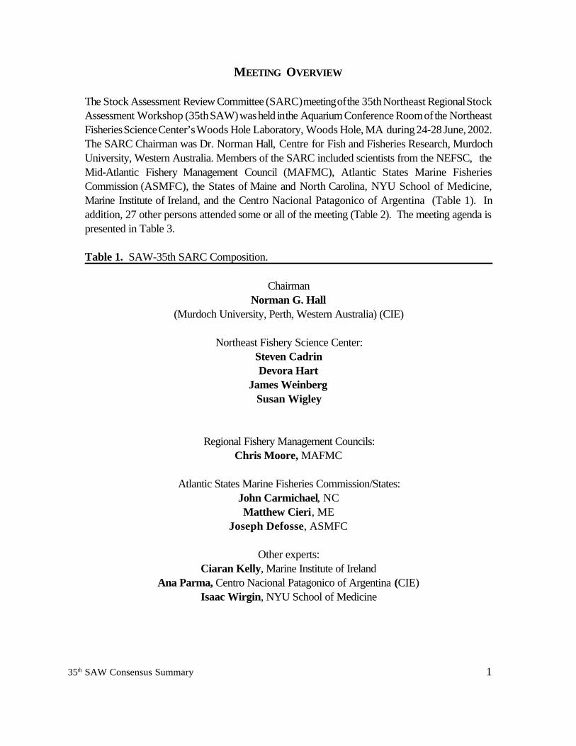
The Stock Assessment Review Committee (SARC) meeting of the 35th Northeast Regional StockAssessment Workshop (35th SAW) was held in the Aquarium Conference Room of the NortheastFisheries Science Center’s Woods Hole Laboratory, Woods Hole, MA during 24-28 June, 2002.The SARC Chairman was Dr. Norman Hall, Centre for Fish and Fisheries Research, MurdochUniversity, Western Australia. Members of the SARC included scientists from the NEFSC, theMid-Atlantic Fishery Management Council (MAFMC), Atlantic States Marine FisheriesCommission (ASMFC), the States of Maine and North Carolina, NYU School of Medicine,Marine Institute of Ireland, and the Centro Nacional Patagonico of Argentina (Table 1). Inaddition, 27 other persons attended some or all of the meeting (Table 2). The meeting agenda ispresented in Table 3.
Table 1. SAW-35th SARC Composition.
ChairmanNorman G. Hall
(Murdoch University, Perth, Western Australia) (CIE)
Northeast Fishery Science Center:Steven CadrinDevora Hart
James WeinbergSusan Wigley
Regional Fishery Management Councils:Chris Moore, MAFMC
Atlantic States Marine Fisheries Commission/States:John Carmichael, NCMatthew Cieri, ME
Joseph Defosse, ASMFC
Other experts:Ciaran Kelly, Marine Institute of Ireland
Ana Parma, Centro Nacional Patagonico of Argentina (CIE) Isaac Wirgin, NYU School of Medicine
2 35th SAW Consensus Summary
Opening
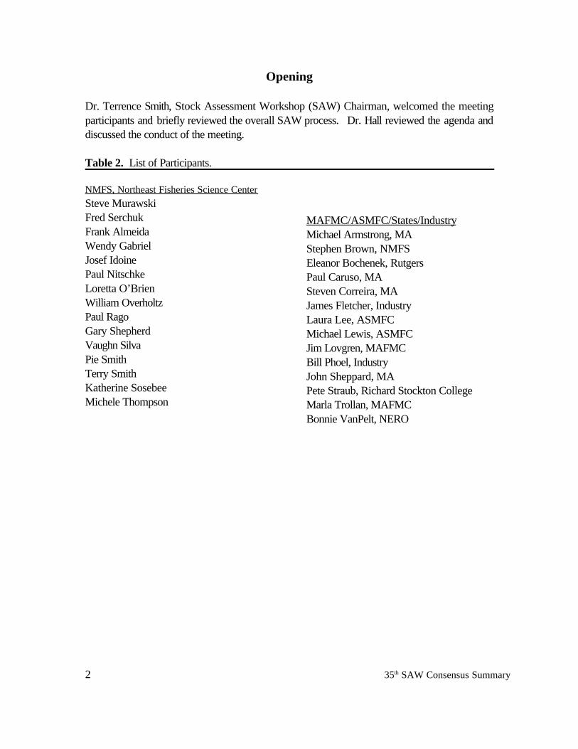
Dr. Terrence Smith, Stock Assessment Workshop (SAW) Chairman, welcomed the meetingparticipants and briefly reviewed the overall SAW process. Dr. Hall reviewed the agenda anddiscussed the conduct of the meeting. Table 2. List of Participants.
NMFS, Northeast Fisheries Science CenterSteve MurawskiFred SerchukFrank AlmeidaWendy GabrielJosef IdoinePaul NitschkeLoretta O’BrienWilliam OverholtzPaul RagoGary ShepherdVaughn SilvaPie SmithTerry SmithKatherine SosebeeMichele Thompson
MAFMC/ASMFC/States/IndustryMichael Armstrong, MAStephen Brown, NMFSEleanor Bochenek, RutgersPaul Caruso, MASteven Correira, MAJames Fletcher, IndustryLaura Lee, ASMFCMichael Lewis, ASMFCJim Lovgren, MAFMCBill Phoel, IndustryJohn Sheppard, MAPete Straub, Richard Stockton CollegeMarla Trollan, MAFMCBonnie VanPelt, NERO

335th SAW Consensus Summary
Table 3. Agenda of the 35th Northeast Regional Stock Assessment Workshop (SAW-35) Stock Assessment Review Committee (SARC) Meeting
Aquarium Conference Room - NEFSC Woods Hole LaboratoryWoods Hole, Massachusetts
24-28 June, 2002
AGENDA
TOPIC WORKING GROUP SARC LEADER RAPPORTEUR& PRESENTER(S)
MONDAY, 24 June (1:00 - 5:00 PM)..................................................................................Opening
Welcome Terry Smith, SAW Chairman P. SmithIntroduction Norm Hall, SARC Chairman
Summer flounder (A) Southern Demersal Working GroupMark Terceiro C. Moore P. Nitschke
TUESDAY, 25 June (8:30 AM - 6:00 PM)..........................................................................Scup (B) Scup Assessment Subcommittee
ASMFC Scup Technical TeamLaura Lee C. Kelly M. Lewis
Informal reception (6:00 PM ) at SWOPE Building (Marine Biological Laboratory)
WEDNESDAY, 26 June (8:30 AM - 5:00 PM).....................................................................8:30 AMMethods Working Group (C) Methods Working Group
Paul Rago A. Parma K. Sosebee1:00 PMWhiting Stock Identification (D) Undersea Research Foundation
Bill Phoel S. CadrinTHURSDAY, 27 June (8:30 AM - 5:00 PM).........................................................................Review Advisory Reports and Consensus Summary Sections for the SARC Report
FRIDAY, 28 June (8:30 AM - 5:00 PM)..............................................................................SARC comments, research recommendations, and 2nd drafts of Advisory ReportsOther business P. Smith* = To be determined by SARC Chairman
4 35th SAW Consensus Summary
The Process
The Northeast Regional Coordinating Council (NRCC) guides the SAW process and is composed of thechief executives of the five partner organizations (NMFS/NEFSC, NMFS/NER, NEFMC, MAFMC,ASMFC). Working groups assemble the data for assessments, decide on methodology, and preparedocuments for SARC review. Assessments for SARC review were prepared at meetings listed in Table4.
Agenda and Reports
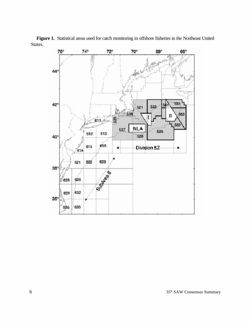
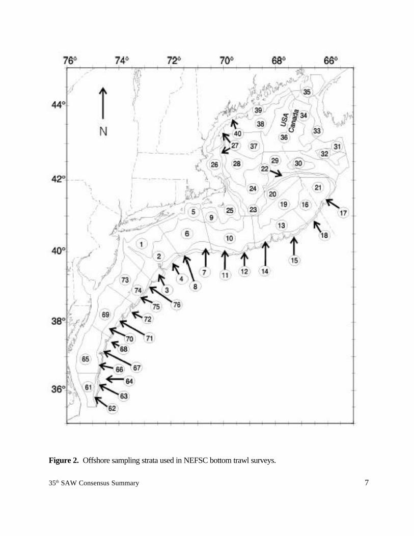
The SAW-35 SARC agenda (Table 3) included presentations on assessments for summer flounder, scup,a review by the SAW Methods Group, and a review of preliminary results from a research studyconcerning silver hake (whiting). A chart of US commercial statistical areas used to report landings in theNorthwest Atlantic is presented in Figure 1. A chart showing the sampling strata used in NEFSC bottomtrawls surveys is presented in Figure 2.
SARC documentation includes two reports: one containing the assessments, SARC comments, andresearch recommendations (SARC Consensus Summary), and another produced in a standard formatwhich includes the status of stocks and management advice (SARC Advisory Report). The draft reportswere made available at a SAW-35 Public Review Workshop held during a joint MAFMC and ASMFCmeeting (6-8 August, Philadelphia). Following the Public Review Workshop, the documents are finalizedand published in the NEFSC Reference Document series as the 35th SARC Consensus Summary ofAssessments (this document) and the 35th SAW Public Review Workshop Report (the latter documentincludes the final version of the Advisory Report).
535th SAW Consensus Summary
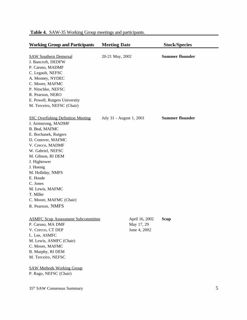
Table 4. SAW-35 Working Group meetings and participants.
Working Group and Participants Meeting Date Stock/Species
SAW Southern Demersal 20-21 May, 2002 Summer flounderJ. Bancroft, DEDFWP. Caruso, MADMFC. Legault, NEFSCA. Mooney, NYDECC. Moore, MAFMCP. Nitschke, NEFSCR. Pearson, NEROE. Powell, Rutgers UniversityM. Terceiro, NEFSC (Chair)
SSC Overfishing Definition Meeting July 31 - August 1, 2001 Summer flounderJ. Armstrong, MADMFB. Beal, MAFMCE. Bochanek, RutgersD. Conover, MAFMCV. Crecco, MADMFW. Gabriel, NEFSCM. Gibson, RI DEMJ. HightowerJ. HoenigM. Holliday, NMFSE. HoudeC. JonesM. Lewis, MAFMCT. MillerC. Moore, MAFMC (Chair)R. Pearson, NMFS
ASMFC Scup Assessment Subcommittee April 16, 2002 ScupP. Caruso, MA DMF May 17, 29V. Crecco, CT DEP June 4, 2002L. Lee, ASMFCM. Lewis, ASMFC (Chair)C. Moore, MAFMCB. Murphy, RI DEMM. Terceiro, NEFSC
SAW Methods Working GroupP. Rago, NEFSC (Chair)
6 35th SAW Consensus Summary
Figure 1. Statistical areas used for catch monitoring in offshore fisheries in the Northeast UnitedStates.
735th SAW Consensus Summary
Figure 2. Offshore sampling strata used in NEFSC bottom trawl surveys.
8 35th SAW Consensus Summary
A. SUMMER FLOUNDER
TERMS OF REFERENCE
The following terms of reference were addressed for summer flounder:
1. Characterize the commercial and recreational catch including landings and discards.
2. Estimate fishing mortality, spawning stock biomass, and total stock biomass for the currentyear and characterize the uncertainty of those estimates.
3. Evaluate and either update or re-estimate biological reference points as appropriate.
4. Where appropriate, estimate a TAC and/or TAL based on stock status and target mortality ratefor the year following the terminal assessment year.
5. If stock projections are possible,
a. provide short term projections (2-3 years) of stock status under various TAC/Fstrategies and
b. evaluate current and projected stock status against existing rebuilding or recoveryschedules, as appropriate.
INTRODUCTION
For assessment purposes, the previous definition of Wilk et al. (1980) of a unit stockextending from Cape Hatteras north to New England has been accepted. The joint Mid-AtlanticFishery Management Council (MAFMC) Atlantic States Marine Fisheries Commission (ASMFC)Fishery Management Plan (FMP) for summer flounder has as a management unit all summerflounder from the southern border of North Carolina, northeast to the U.S.-Canadian border. Arecent summer flounder genetics study (Jones and Quattro, 1999) revealed no significant populationsubdivision centered around Cape Hatteras.
Amendment 1 to the FMP in 1990 established the overfishing definition for summer flounderas fishing mortality rate equal to Fmax, initially estimated as 0.23 (NEFC 1990). Amendment 2 in1992 set target fishing mortality rates for summer flounder for 1993-1995 (F = 0.53) and 1996 andbeyond (Fmax = 0.23). Major regulations enacted under Amendment 2 to meet those fishing mortalityrate targets included: 1) an annual fishery landings quota, with 60% allocated to the commercialfishery and 40% to the recreational fishery, based on the historical (1980-1989) division of landings,with the commercial allocation further distributed among the states based on their share of
935th SAW Consensus Summary
commercial landings during 1980-1989, 2) commercial minimum landed fish size limit at 13 in (33cm), as established in the original FMP, 3) a minimum mesh size of 5.5 in (140 mm) diamond or6.0 in (152 mm) square for commercial vessels using otter trawls that possess 100 lb (45 kg) or moreof summer flounder, with exemptions for the flynet fishery and vessels fishing in an exempted areaoff southern New England (the Northeast Exemption Area) during 1 November to 30 April, 4)permit requirements for the sale and purchase of summer flounder, and 5) annually adjustableregulations for the recreational fishery, including seasons, a 14 in (36 cm) minimum landed fish size,and possession limits.
Amendment 3 to the FMP revised the western boundary of the Northeast Exemption Areato 72030'W (west of Hudson Canyon), increased the large mesh net possession threshold to 200 lbsduring 1 November to 30 April, and stipulated that only 100 lbs could be retained before using alarge mesh net during 1 May to 31 October. Amendment 4 adjusted Connecticut's commerciallandings of summer flounder and revised the state-specific shares of the commercial quotaaccordingly. Amendment 5 allowed states to transfer or combine the commercial quota.Amendment 6 allowed multiple nets on board commercial fishing vessels if properly stowed, andchanges the deadline for publication of overall catch limits and annual commercial managementmeasures to 15 October and the recreational management measures to 15 February.
The results of previous assessments indicated that summer flounder abundance was notincreasing as rapidly as projected when Amendment 2 regulations were implemented. In anticipationof the need to drastically reduce fishery quotas in 1996 to meet the management target of Fmax, theMAFMC and ASMFC modified the fishing mortality rate reduction schedule in 1995 to allow formore stable landings from year to year while slowing the rate of stock rebuilding. Amendment 7 tothe FMP set target fishing mortality rates of 0.41 for 1996 and 0.30 for 1997, with a target of Fmax
= 0.23 for 1998 and beyond. Total landings were to be capped at 8,400 mt (18.51 million lbs) in1996-1997, unless a higher quota in those years provided a realized F of 0.23. Amendment 12 in1999 defined overfishing for summer flounder to occur when the fishing mortality rate exceeds thethreshold fishing mortality rate of FMSY. Since FMSY could not be reliably estimated for summerflounder, Fmax = 0.24 was used as a proxy for FMSY, and was also defined as the target fishingmortality rate. The stock was defined to be overfished when the total stock biomass falls below theminimum biomass threshold of one-half of the biomass target, BMSY. Because BMSY could not bereliably estimated, the biomass target was defined as the product of total biomass per recruit andcontemporary (1982-1996) median recruitment, estimated to be 153,350 mt (338 million lbs), withthe biomass threshold defined as 76,650 mt (169 million lbs). In a recent stock assessment (Terceiro1999), those references points were updated using recent estimates of median recruitment (1982-1998) and mean weights at age (1997-1998), providing a biomass target of 106,444 mt (235 millionlbs) and biomass threshold of 53,222 mt (118 million lbs). The Terceiro (1999) reference pointswere retained in the 2000 and 2001 stock assessments (NEFSC 2000, MAFMC 2001a) because ofthe stability of the input data. Concurrent with the development of the 2001 assessment, theMAFMC and ASMFC convened the ASMFC Summer Flounder Overfishing Definition ReviewCommittee to review the reference points. The work of the Committee was reviewed by theMAFMC Scientific and Statistical Committee (SSC) in August 2001. The SSC recommended thatthe FMSY proxy of Fmax = 0.26 remain for 2002, and endorsed the recommendation of SARC 31
10 35th SAW Consensus Summary
(NEFSC 2000) which stated that “...the use of Fmax as a proxy for FMSY should be reconsidered asmore information on the dynamics of growth in relation to biomass and the shape of the stockrecruitment function become available (MAFMC 2001b).
The 2001 stock assessment (MAFMC 2001a) found that the fishing mortality rate haddeclined from 1.32 in 1994 to 0.30 in 2000, about 15% higher than the FMP overfishing definition.Total stock biomass in 2000 was estimated to be 46,400 mt, 13% below the FMP biomass threshold.Therefore, the stock was found to be overfished and overfishing was occurring relative to the FMPreference points.
FISHERY DATA
Commercial Fishery LandingsTotal U.S. commercial landings of summer flounder from Maine to North Carolina peaked
in 1979 at nearly 18,000 mt (40 million lbs, Table A1). The reported landings in 2001 of 4,916 mt(about 10.8 million lbs) were about 1% over the adjusted 2001 quota of 4,875 mt (10.7 million lbs).Since 1980, 70% of the commercial landings of summer flounder have come from the ExclusiveEconomic Zone (EEZ; greater than 3 miles from shore). The percentage of landings attributable tothe EEZ was lowest in 1983 and 1990 at 63% and was highest in 1989 at 77%. Large variabilityin summer flounder landings exist among the states, over time, and the percent of total summerflounder landings taken from the EEZ has varied widely among the states.
Northeast Region Commercial Fishery LandingsAnnual commercial landings data for summer flounder in years prior to 1994 were obtained
from trip-level detailed landings records contained in master data files maintained by the NEFSC(the weighout system; 1963-1993) and from summary reports of the Bureau of Commercial Fisheriesand its predecessor the U.S. Fish Commission (1940-1962). Beginning in 1994, landings estimateswere derived from mandatory dealer reports under the current NMFS Northeast Region (NER)summer flounder quota monitoring system.
Prior to 1994, summer flounder commercial landings were allocated to NEFSC 3-digitstatistical area according to interview data (Burns et al. In Doubleday and Rivard 1983). For 1994-2001, dealer landings were allocated to statistical area using fishing Vessel Trip Reports (VTR data)according to the general procedures developed by Wigley et al. (1997), in which a matched set ofdealer and VTR data is used as a sample to characterize the statistical area distribution of monthlystate landings. Since the implementation of the annual commercial landings quota in 1993, thecommercial landings have become concentrated during the first calender quarter of the year, withabout 46% of the landings taken during the first quarter in 2001.
The distribution of 1992-2001 landings by three-digit statistical area is presented in TableA2. Areas 537-539 (Southern New England), areas 611-616 (New York Bight), areas 621, 622, 625,and 626 (Delmarva region), and areas 631 and 632 (Norfolk Canyon area) have generally accountedfor over 80% of the NER commercial landings. In 2001, these areas accounted for 95% of the NER
1135th SAW Consensus Summary
commercial landings. A summary of length and age sampling of summer flounder landingscollected by the NEFSC commercial fishery port agent system in the NER is presented in Table A3.For comparability with the manner in which length frequency sampling in the recreational fisheryhas been evaluated, sampling intensity is expressed in terms of metric tons of landings (mt) per 100fish lengths measured. The sampling is proportionally stratified by market category (jumbo, large,medium, small, and unclassified), with the sampling distribution generally reflecting the distributionof commercial landings by market category. Overall sampling intensity has improved markedlysince 1995, from 165 mt per 100 lengths to 30-40 mt per 100 lengths, and temporal and geographiccoverage has generally improved as well.
The age composition of the NER commercial landings for 1994-2001 was generallyestimated semiannually by market category and (usually) 1-digit statistical area (e.g., area 5 or area6), using standard NEFSC procedures (market category length frequency samples converted to meanweights by length-weight relationships; mean weights in turn divided into landings to calculatenumbers landed by market category; market category numbers at length apportioned to age byapplication of age-length keys, on semiannual area basis). For 2000 and 2001, sampling wasgenerally sufficient to make quarterly estimates of the age composition in area 6 (in some cases, bydivision) for the large and medium market categories.
NER landed numbers at age were raised to total NER (general canvas) commercial landingswhen necessary by assuming that landings not accounted for in the weighout/mandatory reportingsystem had the same age composition as that sampled, as follows: calculate proportion at age byweight; apply proportions at age by weight to total NER commercial landings to derive total NERcommercial catch at age by weight; divide by mean weights at age to derive total NER commerciallanded numbers at age (Table A4). The proportion of large and jumbo market category fish in theNER landings has increased since 1996, while the proportion of small market category landings hasbecome very small. The mean size of fish landed in the NER commercial fishery has been increasingsince 1993, and was about 1.01 kg (2.2 lbs) in 2001, typical of an age 3 summer flounder (Table A5).
North Carolina Commercial Fishery LandingsThe North Carolina winter trawl fishery accounts for about 99% of summer flounder
commercial landings in North Carolina. A separate landings at age matrix for this component of thecommercial fishery was developed from North Carolina Division of Marine Fisheries (NCDMF)length and age frequency sampling data. The NCDMF program samples about 10% of the wintertrawl fishery landings annually, at a rate of between 53 and 5 mt of landings per 100 lengthsmeasured (Table A6). All length frequency data used in construction of the North Carolina wintertrawl fishery landings at age matrix were collected in the NCDMF program; age-length keys fromNEFSC commercial data and NEFSC spring survey data (1982-1987) and NCDMF commercialfishery data (1988-2001) were combined by appropriate statistical area and semiannual period toresolve lengths to age. Fishery regulations in North Carolina also changed between 1987 and 1988,with increases in both the minimum mesh size of the codend and minimum landed fish size takingeffect. It is not clear whether the change in regulations or the change in keys, or some combination,is responsible for the decreases in the numbers of age-0 and age-1 fish estimated in the NorthCarolina commercial fishery landings since 1987. Landed numbers at age and mean weights at age
12 35th SAW Consensus Summary
from this fishery are shown in Tables A7-A8.
Commercial Fishery DiscardsIn a previous assessment, analysis of variance of the fishery observer data for summer
flounder was used to identify stratification variables for an expansion procedure to estimate totallandings and discards from fishery observer data kept and discard rates (weight per day fished) inthe commercial fishery. Initial models included year, quarter, fisheries statistical division (2-digitarea), area (divisions north and south of Delaware Bay), and tonnage class as main effects, withquarter and division emerging (along with year) as consistently significant main effects withoutsignificant interaction with the year (NEFSC 1993). The estimation procedure expandstransformation bias-corrected geometric mean catch (landings and discards) rates in year, quarter,and division strata by total days fished (days fished on trips landing any summer flounder by anymobile gear, including fish trawls and scallop dredges) to estimate fishery landings and discards.The use of fishery effort as the multiplier (raising factor) allows estimation of landings from thefishery observer data for comparison with dealer reported landings, to help judge the potentialaccuracy of the procedure and/or sample data.
For strata with no fishery observer sampling, catch rates from adjacent or comparable stratawere substituted as appropriate (except for Division 51, which generally has very low catch rates andnegligible catch). Estimates of discard are stratified by 2 gear types (scallop dredge and trawl andothers) for years when data are adequate (1992-2001). Estimates at length and age are stratified bygear only for 1994-2000, again due to sample size considerations. Only 11 fish were sampled fromthe sea scallop dredge fishery 2001, and so the scallop dredge discards were assumed to have thesame length and age composition as the trawl fishery discards in 2001.
While estimates of catch rates from the NER fishery observer data are used in this assessmentto estimate total discards, information on catch rate is also reported in the VTR data. A comparisonof discard to total catch ratios for the fishery observer and VTR data sets for trawl and scallop dredgegear indicated similar discard rates in the trawl fishery from the two data sources, while discard ratesin the scallop dredge fishery were often higher in the fishery observer data. Overall fishery observerand VTR discard to total catch ratios for 1994-2000 were generally within 10% of each other; 2001was an exception, with an overall discard to total catch ratio of 45% in the fishery observer data and29% in the VTR data (Tables A9-A10).
The change from the interview/weighout data reporting system to the VTR/mandatory dealerreport system required a change in the estimation of effort (days fished) used as a multiplier with thefishery observer geometric mean discard rate in the procedure used to estimate total discard for1994-2001. An initial examination of days fished and catch per unit effort (CPUE; landings per dayfished) for cod conducted at SAW 24 (NEFSC 1997a) compared these quantities as reported in thefull weighout and VTR data sets (DeLong et al., 1997). This comparison indicated a shift to a higherfrequency of short trips (trips with one or two days fished reported), and to a mode at a lower rateof CPUE. It was not clear at SAW 24 if these changes were due to the change in reporting system(units reported not comparable), or real changes in the fishery, and so effort data reported by theVTR system were not used quantitatively in the SAW 24 assessments. In the SAW 25 assessment
1335th SAW Consensus Summary
for summer flounder (NEFSC 1997a), a slightly different comparison was made. The port agentinterview data for 1991-93 and merged dealer/VTR data for 1994-1996 (the matched set data), whichunder each system serve as the “sample” to characterize the total commercial landings, werecompared in relative terms (percent frequency). For summer flounder, the percent frequency of shorttrips (lower number of days fished per trip) increased during 1991-1996, but not to the degreeobserved for cod, and the mode of CPUE rates for summer flounder increased in spite of lowereffort per trip. For the summer flounder fishery, these may reflect actual changes in the fishery, dueto increasing restrictions of allowable landings per trip (trip landings limits might lead to shortertrips) and increasing stock size (higher CPUE). As for cod, however, the influence of each of thesechanges (reporting system, management changes, stock size changes) has not been quantified. Totaldays fished in the summer flounder fishery were comparable between 1989-1993 period and 1994.With increasing restrictions on the fishery in 1995-2001 (lower landings quota, higher stock size,and thus increasing impact of trips limits and closures), total days fished declined relative to the early1990s. Questions will remain about the accuracy of the VTR data . However, because the effortmeasure is critical to the estimation of discards for summer flounder, the VTR data were used as thebest data source to estimate summer flounder fishery days fished for 1994-2001.
Two adjustments were made to the dealer/VTR matched data subset days fished estimatesto fully accounted for summer flounder fishery effort during 1994-2001. First, the landings to daysfished relationship in the matched set was assumed to be the same for unmatched trips, and so thedays fished total in each discard estimation stratum (2-digit area and quarter) was raised by the dealerto matched set landings ratio. This step in the estimation accounted for days fished associated withtrips landing summer flounder, and provided an estimate of discard for trips landing summerflounder.
Given the restrictions on the fishery however, there is fishing activity which results insummer flounder discard, but no landings, especially in the scallop dredge fishery. The days fishedassociated with these trips was accounted for by raising strata discard estimates by the ratio of thetotal days fished on trips catching any summer flounder (trips with landings and discard, plus tripswith discard only) to the days fished on trips landing summer flounder (trips with landings anddiscard), for VTR trips reporting discard of any species (DeLong et al. 1997). For this step, it isnecessary to assume that the discard rate (as indicated by the fishery observer data, which includestrips with discard but no landings, and which is used in previous estimation procedure steps) is thesame for trips with only discard as for trips which both land and discard.
The expansion procedure provided fishery observer data estimates of landings ranging from+35% (1996) to -69% (2001) of the reported landings in the fisheries, with discard ranging from 41%(1990) to 6% (1995) of the reported landings. Total discards estimated for 2000 and 2001 were 18%and 16% of the reported landings. Scallop dredge fishery discard to landed ratios are much higherthan trawl fishery ratios, purportedly because of closures and trip limits. Thus, although the scallopdredge landings are less than 5% of the total, the discard is of the same order of magnitude as thatin the trawl fishery.
These discard estimates were based only on the days fished data for ports in the NER during
14 35th SAW Consensus Summary
1989-1996, and so it was necessary to raise the discard estimate to account for discarding whichoccurs in components of the commercial fishery outside the NER reporting system (i.e., NER statereporting systems such as Connecticut and Virginia, and North Carolina) for those years. Todetermine the proper raising factor, landings accounted for by the NER reporting system (whichresult from the fishing effort on which the fishery observer discard estimate is based) were comparedwith total NER landings, plus that portion of North Carolina landings removed from the EEZ (it isassumed that only the North Carolina fishery in the EEZ would experience significant discard, asmesh regulations in state waters have resulted in very low discards in state waters sinceimplementation of the regulation in 1989; R. Monaghan, pers. comm.). Since 1996, all states’landings and are included in the NER dealer reporting system, so no raising is necessary to accountfor missing landings. As recommended by SAW 16 (NEFSC 1993), a commercial fishery discardmortality rate of 80% was assumed to develop the final estimate of discard mortality (Table A11).
Existing fishery observer data were used to develop estimates of commercial fishery discardfor 1989-2001. However, adequate data (e.g., interviewed trip data, survey data) are not availablefor summer flounder to develop discard estimates for 1982-1988. Discard numbers were assumedto be very small relative to landings during 1982-1988 (because of the lack of a minimum size limitin the EEZ), but to have increased since 1989 with the implementation of fishery regulations underthe FMP. It is recognized that not accounting directly for commercial fishery discards would resultin an underestimation of fishing mortality and population sizes in 1982-1988.
NEFSC fishery observer length frequency samples were converted to sample numbers at ageand sample weight at age frequencies by application of NEFSC survey length-weight relationshipsand fishery observer, commercial fishery, and survey age-length keys. Sample weight proportionsat age were next applied to the raised fishery discard estimates to derive fishery total discard weightat age. Fishery discard weights at age were then divided by fishery observer mean weights at ageto derive fishery discard numbers at age. Classification to age for 1989-1993 was done bysemiannual (quarters 1 and 2 pooled, quarters 3 and 4 pooled) periods using NEFSC fishery observerage-length keys, except for 1989, when first period lengths were aged using combined commercial(quarters 1 and 2) and NEFSC spring survey age-length keys. For 1994-2001, only NEFSC winter,spring, and fall survey age-length keys were used. Fishery observer sampling intensity issummarized in Table A11. Estimates of discarded numbers at age, mean length and mean weightat age are summarized in Tables A12-A14.
The reason for discarding in the trawl and scallop dredge fisheries has been changing overtime. During 1989 to 1995, the minimum size regulation was recorded as the reason for discardingsummer flounder for over 90% of the observed trawl and scallop dredge tows. In 1999, the minimumsize regulation was provided as the reason for discarding for 61% of the observed trawl tows, withquota or trip limits given as the discard reason for 26% of the observed tows, and high-grading for11% of the observed tows. In the scallop fishery in 1999, quota or trip limits was given as thediscard reason for over 90% of the observed tows. During 2000-2001, minimum size regulationswere identified as the discard reason for 40-45% of the observed trawl tows, quota or trip limits for25-30% of the tows, and high grading for 3-8%. In the scallop fishery during 2000-2001, quota ortrip limits was given as the discard reason for over 99% of the observed tows. As a result of the
1535th SAW Consensus Summary
increasing impact of trip limits, fishery closures, and high grading as the reasons for discarding, theage structure of the summer flounder discards has also changed, with more older fish being discarded(Table A12). Recreational Fishery Landings
Summary landings statistics for the recreational fishery (catch type A+B1) as estimated bythe National Marine Fisheries Service (NMFS) Marine Recreational Fishery Statistics Survey(MRFSS) are presented in Tables A15-A16. Recreational fishery landings decreased 29% bynumber and 26% by weight from 2000 to 2001, although the fishery still landed 162% (5,250 mt,11.6 million lbs) of the 3,250 mt (7.2 million lbs) harvest limit established for 2001.
The length frequency sampling intensity for the recreational fishery for summer flounder wascalculated by MRFSS subregions (North - Maine to Connecticut; Mid - New York to Virginia; South- North Carolina) on a metric tons of landings per hundred lengths measured basis (Burns et al. InDoubleday and Rivard, 1983). For 2001, aggregate sampling intensity averaged 123 mt of landingsper 100 fish measured, an improvement over 2000 (Table A17).
MRFSS sample length frequency data, NEFSC commercial age-length data, and NEFSCsurvey age-length data were examined in terms of number of fish measured/aged on various temporaland geographical bases. Correspondences were made between MRFSS intercept date (quarter),commercial quarter, and survey season (spring and summer/fall) on temporal bases, and betweenMRFSS subregion, commercial statistical areas, and survey depth strata on geographic bases in orderto integrate data from the different sources. Based on the number, size range, and distribution oflengths and ages, a semiannual (quarters 1 and 2, quarters 3 and 4), subregional basis of aggregationwas adopted for matching of commercial and survey age-length keys with recreational lengthfrequency distributions for conversion of the lengths to ages.
The recreational landings historically have been dominated by relatively young fish. Overthe 1982-1996 period, age 1 fish accounted for an average of over 50% of the landings by number;summer flounder of ages 0 to 4 accounted for an average of over 99% of landings by number. Nofish from the recreational landings were determined to be older than age 7. With increases in theminimum size during 1997-2001 (to 14.5 in [37 cm] in 1997, 15 in [38 cm] in 1998-1999, generally15.5 in [39 cm] in 2000, and various state minimum sizes from 15.5 [38 cm] to 17.5 in [44 cm] in2001), reductions in fishing mortality, and patterns in recruitment to the stock, the age compositionof the recreational landings now includes mainly fish at ages 2 and 3. The number of summerflounder of ages 4 and older landed by the recreational fishery in 2000 (11% of the landings bynumber) and 2001 (13%) was the highest since 1983 (Table A18).
Small MRFSS intercept length sample sizes for larger fish resulted in a high degree ofvariability in mean length for older fish, especially at ages 5 and older. Attempts to estimate length-weight relationships from MRFSS biological sample data for use in estimating weight at ageprovided unsatisfactory results. As a result, quarterly length (mm) to weight (g) relationships fromLux and Porter (1966), which are employed in the conversion of length to weight in NEFSCcompilation of commercial fishery statistics for summer flounder, were used to calculate annual
16 35th SAW Consensus Summary
mean weights at age from the estimated age-length frequency distribution of the landings.
Recreational Fishery DiscardsMRFSS catch estimates were aggregated on a subregional basis for calculation of the
proportion of live discard (catch type B2) to total catch (catch types A+B1+B2) in the recreationalfishery for summer flounder. Examination of catch data in this manner shows that the live discardhas varied from about 18% (1985) to about 81% (1999, 2001) of the total catch (Table A19).
To account for all removals from the summer flounder stock by the recreational fishery, someassumptions about the biological characteristics and hooking mortality rate of the recreational livediscard needed to be made, because no biological samples are taken from MRFSS catch type B2.In previous assessments, data available from New York Department of Environmental Conservation(NYDEC) surveys (1988-92) of New York party boats suggested the following for this component(Mid-Atlantic subregion, anglers fishing from boats) of the recreational fishery: 1) nearly all (>95%)of the fish released alive were below the minimum regulated size (during 1988-92, 14 in [36 cm] inNew York state waters), 2) nearly all of these fish were age 0 and age 1 summer flounder, and 3)age 0 and 1 summer flounder occurred in approximately the same proportions in the live discard asin the landings. It was assumed that all B2 catch would be of lengths below regulated size limits,and so either age 0 or age 1 in all three subregions during 1982-1996. Catch type B2 was thereforeallocated on a subregional basis in the same ratio as the annual age 0 to age 1 proportion observedin the landings during 1982-1996. Mean weights at age were assumed to be the same as in thelandings during 1982-1996.
The minimum landed size in federal and most state waters increased to 14.5 in (37 cm) in1997, to 15.0 in (38 cm) in 1998-1999, and to 15.5 in (39 cm) in 2000. Applying the same logicemployed to classify the 1982-1996 recreational released catch to size and age for 1997-2000 impliedthat the recreational fishery released catch included fish of ages 2 and 3. Investigation of data fromthe CTDEP Volunteer Angler Survey (VAS, 1997-1999) and American Littoral Society (ALS,1999), comparing the length frequency of released fish in those programs with the MRFSS data onthe length frequency of landed fish less than the minimum size, suggested this assumption was validfor 1997-1999 (MAFMC 2001a). The CTDEP VAS and ALS data, along with data from theNYDEC Party Boat Survey (PBS) was used to validate this assumption for 2000. For 1997-2000it was therefore assumed that all B2 catch would be of lengths below regulated size limits, and soof ages 0 to 3. Catch type B2 was therefore allocated on a sub-regional basis in the same ratio as theannual age 0 to age 3 proportions observed in the landings at lengths less than 37 cm in 1997, 38cm in 1998-1999, and 39 cm in 2000 (Table A20).
In 2001, many states adopted different combinations of minimum size and possession limitsto meet management requirements. As a result, minimum sizes for summer flounder ranged from15.5 in (39 cm) in Federal, VA, and NC waters, 16 in (41 cm) in NJ, 16.5 in (42 cm) in MA, 17 in(43 cm) in MD and NY, to 17.5 in (44 cm) in CT, RI, and DE. Examination of data provided by MDsport fishing clubs, the CTDEP VAS, the ALS, and the NYDEP PBS indicated that the basicassumption that fish released are those smaller than the minimum size remained valid. Thus for2001, catch type B2 was characterized by the same proportion at length as the landed catch less than
1735th SAW Consensus Summary
the minimum size in the respective states. Due to sample size considerations, lengths and B2 catchwere aggregated to semi-annual, subregional strata to calculate the expanded discards at length. Thenumber of age 1 fish discarded in the recreational fishery in 2001 was the most since 1996 (TableA20).
Studies conducted cooperatively by NEFSC and the state of Massachusetts to estimatehooking mortality for striped bass and black sea bass suggest a hooking mortality rate of 8% forstriped bass (Diodati and Richards 1996) and 5% for black sea bass (Bugley and Shepherd, 1991).Work by the states of Washington and Oregon with Pacific halibut (a potentially much larger flatfishspecies, but otherwise morphologically similar to summer flounder) found "average hookingmortality...between eight and 24 percent" (IPHC, 1988). An unpublished tagging study by theNYDEC (Weber MS 1984) on survival of released sublegal summer flounder caught by hook-and-line suggested a total, non-fishing mortality rate of 53%, which included hooking plus taggingmortality as well as deaths by natural causes (i.e., predation, disease, senescence). Assuming deathsby natural causes to be about 18%, (an instantaneous rate of 0.20), an annual hooking plus taggingmortality rate of about 35% can be derived from the NYDEC results. In the SARC 25 (NEFSC1997b) and earlier assessments of summer flounder, a 25% hooking mortality rate was assumedreasonable for summer flounder released alive by anglers.
Two more recent investigations of summer flounder recreational fishery release mortalitysuggest that a lower release mortality rate is appropriate. Lucy and Holton (1998) used field trialsand tank experiments to investigate the release mortality rate for summer flounder in Virginia, andfound rates ranging from 6% (field trials) to 11% (tank experiments). Malchoff and Lucy (1998)used field cages to hold fish angled in New York and Virginia during 1997 and 1998, and found amean short term mortality rate of 14% across all trials. Given the results of these release mortalitystudies conducted specifically for summer flounder, a 10% release mortality rate was adopted in theTerceiro (1999) and has been retained in subsequent assessments (NEFSC 2000, MAFMC 2001a).
Ten percent of the total B2 catch at age is added to estimates of summer flounder landingsat age to provide estimates of summer flounder recreational fishery discard at age (Table A20), totalrecreational fishery catch at age in numbers (Table A21) and mean weights at age (Table A22). Thenumber of fish discarded and assumed dead in the recreational fishery (2.3 million fish, 1,184 mt)was 43% by number and 23% by weight of the total landed (5.2 million fish, 5,250 mt) in therecreational fishery in 2001.
Total Catch CompositionNER total commercial fishery landings and discards at age, North Carolina winter trawl
fishery landings and discards at age, and MRFSS recreational fishery landings and discards at agetotals were summed to provide a total fishery catch at age matrix for 1982-2001 (Table A23; FigureA1). The percentage of age-3 and older fish in the total catch in numbers has increased in recentyears from only 4% in 1993, to about 40% during 1998-2001. Overall mean lengths and weights atage for the total catch were calculated as weighted means (by number in the catch at age) of therespective mean values at age from the NER commercial (Maine to Virginia), North Carolina
18 35th SAW Consensus Summary
commercial, and recreational (Maine to North Carolina) fisheries (Tables A24-A25; Figure A2). Therecreational fishery share of the total summer flounder catch has increased since 1995 (Figure A3).
BIOLOGICAL DATA
AgingWork performed for the SAW 22 assessment (NEFSC 1996b) indicated a major expansion
in the size range of 1-year old summer flounder collected during the 1995 and 1996 NEFSC winterbottom trawl surveys, and brought to light differences between ages determined by the NEFSC andNCDMF fishery biology staffs. Age structure (scale) exchanges were performed after the SAW 22assessment to explore these aspects of summer flounder biology. The results of the first twoexchanges, which were reported at SAW 22 (NEFSC 1996b), indicated low levels of agreementbetween age readers at the NEFSC and NC DMF (31 and 46%). In 1996, research was conductedto determine inter-annular distances and to back-calculate mean length at age from scale samplescollected on all NEFSC bottom trawl surveys (winter, spring and fall) in order to compare withNCDMF samples. While mean length at age remained relatively constant from year to year, inter-annular distances increased sharply in the samples from the 1995-1996 winter surveys, and increasedto a lesser degree in samples from other 1995-1996 surveys as well. As a result, further exchangeswere suspended pending the resolution of an apparent aging problem.
Age data from the winter 1997 bottom trawl survey, aged utilizing both scales and otolithsby only by one reader, indicated a similar pattern as the previous two winter surveys (i.e., severallarge age 1 individuals) from scale readings, and some disagreement between scale and otolith agesobtained from the same fish. Because of these problems, a team of five experienced NEFSC readerswas formed to re-examine the scales aged from the winter survey. After examining several hundredscales, the team determined that re-aging all samples from 1995-1997, including all winter, spring,and fall samples from the NEFSC and MA DMF bottom trawl surveys and all samples from thecommercial fishery, would be appropriate. The age determination criteria used remained the sameas developed at the 1990 summer flounder workshop (Almeida et al. 1992) and described in thestandard aging manual utilized by NEFSC staff (Dery 1997). Only those fish for which a 100%consensus of all group members could be reached were included in the revised database, however.The data from the re-aged database were used in analyses in the SAW 25 assessment (NEFSC1997b).
A third summer flounder aging workshop was held at NEFSC in February, 1999, to continuethe exchange of age structures and review of aging protocols for summer flounder (Bolz et al. 2000).The participants of the latest workshop concluded that the majority of aging disagreements in recentNEFSC-NCDMF exchanges arose from the interpretation of marginal scale increments due to highlyvariable timing of annulus formation, and from the interpretation of first year growth patterns andfirst annulus selection. The workshop recommended regular samples exchanges between NEFSCand NCDMF, and further analyses of first year growth.
1935th SAW Consensus Summary
MaturityThe maturity schedule for summer flounder used in the 1990 SAW 11 and subsequent stock
assessments through 1999 was developed by the SAW 11 Working Group using NEFSC Fall Surveymaturity data for 1978-1989 and mean lengths at age from the NEFSC fall survey (G. Shepherd,NEFSC, personal communication; NEFC 1990; Terceiro 1999). The SAW 11 work indicated thatthe median length at maturity (50th percentile, L50) was 25.7 cm for male summer flounder and 27.6cm for female summer flounder, and 25.9 cm for the sexes combined. Under the aging conventionused in the SAW 11 and subsequent assessments (Smith et al. 1981, Almeida et al. 1992,Szedlmayer and Able 1992, Bolz et al. 2000), the median age of maturity (50th percentile, A50) forsummer flounder was determined to be 1.0 years for males and 1.5 years for females. Combinedmaturities indicated that 38% of age-0 fish are mature, 72% of age-1 fish are mature, 90% of age-2fish are mature, 97% of age-3 fish are mature, 99% of age-4 fish are mature, and 100% of age-5 andolder fish are mature at peak spawning time in the autumn. The maturities for age-3 and older wererounded to 100% in the SAW 11 and subsequent assessments.
In the series of summer flounder assessments, it has been noted that the maturity scheduleshave been based on simple gross morphological examination of the gonads and therefore may notaccurately reflect (i.e., may overestimate) the true spawning potential of the summer flounder stock(especially for age-0 and age-1 fish). It should also be noted, however, that spawning stock biomass(SSB) estimates based on age-2 and older fish show the same long term trends in SSB as estimateswhich include age 0 and 1 fish in the spawning stock. A research recommendation that the truespawning contribution of young summer flounder to the SSB be investigation has been included insummer flounder stock assessments since 1993 (NEFSC 1993). In light of the completion of a URIstudy to address this research recommendation, the maturity data for summer flounder for 1982-1998were examined in the 2000 assessment (NEFSC 2000) to determine if changes in the maturityschedule were warranted.
The research at the University of Rhode Island (URI) by Drs. Jennifer Specker and RebeccaRand Merson (hereafter referred to collectively as the “URI 1999" study) attempted to address theissue of the true contribution of young summer flounder to the spawning stock. The URI 1999study examined the histological and biochemical characteristics of female summer flounder oocytes(1) to determine if age-0 and age-1 female summer flounder produce viable eggs, and (2) to developan improved guide for classifying the maturity of summer flounder collected in NEFSC surveys(Specker et al. 1999, Merson et al. In press, Merson et al. In review). The URI study examined 333female summer flounder (321 aged fish) sampled during the NEFSC Winter 1997 Bottom TrawlSurvey (February 1997) and 227 female summer flounder (210 aged fish) sampled during theNEFSC Autumn 1997 Bottom Trawl Survey (September 1997), using radioimmunoassays toquantify the biochemical cell components characteristic of mature fish.
To provide an increased sampled size for the calculation of length- and age-based maturityschedules, the fish in the URI study sampled from the NEFSC Winter and Autumn 1997 Surveyswere combined, with the ages of the fish from the Winter Survey reduced by 1 year to reflect theirage at spawning during the previous (1996) autumn. For this combined sample, the NEFSC and URImaturity criteria disagreed for 13% of the aged fish, with most (10%) of the disagreement due to
20 35th SAW Consensus Summary
NEFSC mature fish classified as immature by the URI histological and biochemical criteria. Of the531 female summer flounder in the combined age sample, the URI criteria indicated that 15% of theage-0 fish were mature, 82% of the age-1 fish were mature, 97% of the age-2 fish were mature, and100% of the age 3 and older fish were mature. When the proportions of fish mature at length andage were estimated by probit analysis, the URI 1999 criteria a median length at maturity (50th
percentile, L50) of 34.7 cm for female summer flounder, with proportions mature at age of age-0:30%, age-1: 68%, age-2: 92%, age-3: 98%, age-4: 100%., with a median age of maturity (50th
percentile, A50) of about 0.5 years.
SARC 31 (NEFSC 2000) considered 5 options for the summer flounder maturity schedulefor the 2000 stock assessment:
1) No change, use the maturity schedule for combined sexes as in the SAW 11 andsubsequent assessments (the schedule presented below is rounded to 0.38, 0.72, 0.90,1.00, 1.00, and 1.00 as in the SAW 25 and Terceiro (1999) assessment analyses).
2) Consider only age-2 and older fish of both sexes in the SSB.
3) Knife edged, age-1 and older maturity for both sexes. This would eliminate age-0 fishof both sexes from the SSB, and assume that the proportions mature at age-1 “round”to 100%.
4) NEFSC 1982-1989, 1990-1998 for both sexes, assuming a 1:1 sex ratio to averageproportions for a combined schedule.
5) NEFSC 1982-1989, 1990-1998 for males, URI 1999 for females, assuming a 1:1 sex ratioto average proportions for a combined schedule.
SARC 31 concluded that some contribution to spawning from ages 0 and 1 should beincluded, eliminating options 2 and 3. The differences among remaining options 1, 4, and 5 wereconsidered to be relatively minor, and so the SAW 11 schedule (Option 1) was retained for the 2000(NEFSC 2000), 2001 (MAFMC 2001a), and current (2002) assessment. SARC 31 recommendedthat more biochemical and histological work, for both male and female summer flounder, should bedone for additional years to determine if the results of the URI 1999 study will be applicable overthe full VPA time series. SARC 31 also noted the need for research to explore whether the viabilityof eggs produced by young, first time spawning summer flounder is comparable to the viability ofeggs produced by older, repeat spawning summer flounder.
RESEARCH SURVEY ABUNDANCE AND BIOMASS INDICES
NEFSC SpringLong-term trends in summer flounder abundance were derived from a stratified random
bottom trawl survey conducted in spring by NEFSC between Cape Hatteras and Nova Scotia since
2135th SAW Consensus Summary
1968 (Clark 1978). NEFSC spring survey indices (Tables A26-A27) suggest that total stock biomasslast peaked during 1976-1977, and in 2002 was now about 15% above that peak, and at a newhistorical high (Figure A4). Age composition data from the NEFSC spring survey indicate asubstantial reduction in the number of ages in the stock between 1976-1990 (Table A27). Between1976-1981, fish of ages 5-8 were captured regularly in the survey, with the oldest individuals aged8-10 years. Between 1982-1986, fish aged 5 and older were only occasionally observed in thesurvey, and by 1986, the oldest fish observed in the survey were age 5. In 1990 and 1991, only threeages were observed in the survey catch, and there was an indication that the 1988 year class was veryweak. Since 1991, the survey age composition has expanded significantly. There is strong evidencein the 1998-2002 NEFSC spring surveys of increasing abundance of age-3 and older fish, due toincreased survival of the 1994 and subsequent year classes (Table A27). Mean lengths at age in theNEFSC spring survey are presented in Table A28.
NEFSC AutumnSummer flounder are caught frequently in the NEFSC autumn survey at stations in the
inshore strata (< 27 meters = 15 fathoms = 90 feet) and in the band of offshore strata of 27-55 metersdepth (15-30 fathoms, 90-180 feet), at about the same magnitude as in the spring survey (Table A26).Furthermore, the autumn survey catches age-0 summer flounder in abundance, providing an indexof summer flounder recruitment (Tables A29 & A48, Figure A7). Fall survey indices suggestimproved recruitment since the late 1980s, and evidence of an increase in abundance at age-2 andolder since 1995. The NEFSC autumn surveys indicate that the 1995 year class of summer flounderwas the most abundant in recent years, and that subsequent, weaker year classes are experiencingincreased survival (Table A29). Mean lengths at age in the NEFSC autumn survey are presentedin Table A30.
NEFSC WinterA new series of NEFSC winter trawl surveys was begun in February 1992 specifically to
provide improved indices of abundance for flatfish, including summer flounder. This survey targetsflatfish during the winter when they are concentrated offshore. A modified 36 Yankee trawl is usedin the winter survey that differs from the standard trawl employed during the spring and autumnsurveys in that 1) long trawl sweeps (wires) are added before the trawl doors, to better herd fish tothe mouth of the net, and 2) the large rollers used on the standard gear are absent, and only a chain"tickler" and small spacing "cookies" are present on the footrope.
Based on a comparison of summer flounder catches during the winter surveys with recentspring and autumn surveys, the design and conduct of the winter survey (timing, strata sampled, andthe use of the modified 36 Yankee trawl gear) has resulted in greater catchability of summer floundercompared to the other surveys. Most fish have been taken in survey strata 61-76 (27-110 meters; 15-60 fathoms), off the Delmarva and North Carolina coasts . Other concentrations of fish are foundin strata 1-12, south of the New York and Rhode Island coasts, in slightly deeper waters. Significantnumbers of large summer flounder are often captured along the southern flank of Georges Bank(strata 13-18).
Indices of summer flounder abundance from the winter survey indicated stable stock sizeduring 1992-1995, with indices of stratified mean catch per tow in number ranging from 10.9 in
22 35th SAW Consensus Summary
1995 to 13.6 in 1993. The NEFSC winter survey index for 1996 increased by 290% over the 1995value, from 10.8 to 31.2 fish per tow. The largest increases in 1996 catch per tow occurred in theMid-Atlantic Bight region (offshore strata 61-76), where increases in catch per tow of up to an orderof magnitude over the 1995 level occurred in several strata, with the largest increases in strata 61,62,and 63, off the northern coast of North Carolina. Most of the increased catch in 1996 consisted ofage-1 summer flounder from the 1995 year class. In 1997, the index dropped to 10.3 fish per tow,due to the lower numbers of age-1 (1996 year class) fish caught. The Winter 2002 survey kg pertow index is the highest of the 1992-2002 series (Tables A26 & A31, Figure A4). As with the othertwo NEFSC surveys, there is strong evidence in recent winter surveys of increased abundance ofage-3 and older fish relative to earlier years in the time series, due to the abundance of the 1995 yearclass and increased survival of subsequent year classes (Table A32). Mean lengths at age in theNEFSC winter survey are presented in Table A33.
Massachusetts DMFSpring and fall bottom trawl surveys conducted by the Massachusetts Division of Marine
Fisheries (MADMF) show a decline in abundance in numbers of summer flounder from recent highlevels in 1986 to record lows in 1990 (MADMF fall survey), and 1991 (MADMF spring survey).In 1994, the MADMF survey indices increased to values last observed during 1982-1986, but thendeclined substantially in 1995, although the indices remain higher than the levels observed in the late1980s . Since 1996, both the MADMF spring and fall indices have increased substantially to valueslast observed during 1982-1986 (Tables A34-A35, Figure A5). The MADMF also captures a smallnumber of age-0 summer flounder in a seine survey of estuaries, and these data are available as anindex of recruitment (Tables A36 & A48, Figure A9).
Connecticut DEPSpring and fall bottom trawl surveys are conducted by the Connecticut Department of
Environmental Protection (CTDEP). The CTDEP surveys show a decline in abundance in numbersof summer flounder from high levels in 1986 to record lows in 1989. The CTDEP surveys indicaterecovery since 1989, and evidence of increased abundance at ages 2 and older since 1995. The 2000and 2001 spring indices were the highest of the 16 year time series, and the 2001 autumn index wasthe highest of the series (Tables A37-A38, Figure A6). An index of recruitment from the autumnseries is available (Tables A38 & A48, Figure A7).
Rhode Island DFWA standardized bottom trawl survey has been conducted during the spring and fall months
in Narragansett Bay and state waters of Rhode Island Sound by the Rhode Island Department of Fishand Wildlife (RIDFW) since 1979. Indices of abundance at age for summer flounder have beendeveloped from the autumn survey data using NEFSC autumn survey age-length keys. The 1988and 1991 year classes are the weakest in recent years in this time series, and the index shows the1984-1987, 1999, and 2000 year classes to have been the strongest. The autumn survey was at ornear a time-series high during 1999-2000 (Table A39, Figure A5). A new series of indices wasdeveloped from a set of fixed stations sampled monthly during 1990-2000. Age-1 indices from thisseries indicate that strong year classes recruited to the stock in1996, 1999, and 2000, with age 2+abundance peaking in 2000 (Table A40). Recruitment indices are available from both the autumn
2335th SAW Consensus Summary
and monthly fixed station surveys (Table A39-A40 & A48, Figure A9).
New Jersey BMFThe New Jersey Bureau of Marine Fisheries (NJBMF) has conducted a standardized bottom
trawl survey since 1988. Indices of abundance for summer flounder incorporate data collected fromApril through October. NJBMF supplied annual total mean number per tow indices and associatedannual length frequency distributions; lengths were converted to age using the corresponding annualNEFSC combined spring and fall survey age-length keys. Indices of the 1995 year class at age-0 andat older ages in subsequent years through 1999 indicate that it is the strongest of the 1988-2001 timeseries. Indices of the 1996-2001 year classes are below the time series average. The NJBMF surveyindices show evidence of increased abundance at age-2 and older in the 1995-2000 surveys, but adecline in 2001 (Table A41, Figure A6). Recruitment indices are available from the NJBMF survey(Tables A41 & A48, Figure A7).
Delaware DFWThe Delaware Division of Fish and Wildlife (DEDFW) has conducted a standardized bottom
trawl survey with a 16 foot headrope trawl since 1980, and with a 30 foot headrope trawl since 1991.Recruitment indices (age 0 fish; one index from the Delaware estuary proper, one from the inlandbays) have been developed from the 16 foot trawl survey data for the 1980 to 2001 year classes.Indices for age-0 to age-4 and older summer flounder have been compiled from the 30 foot headropesurvey. The indices incorporate data collected from June through October (arithmetic mean numberper tow), with age 0 summer flounder separated from older fish by visual inspection of the lengthfrequency. The 16 foot headrope survey indices suggest poor recruitment in 1988 and 1993, andimproved recruitment in 1994-1995 (Tables A42-A43 & A48). The 16-foot trawl Estuary indexindicates below average recruitment since 1995, except for 2000 (Figure A9). The 16-foot trawlInland Bays index indicates above average recruitment during 1998-2000, and poor recruitment in2001. The 30 foot headrope survey indices suggest stable stock sizes over the 1991-2001 time series,with strong recruitment in 1991, 1994, 1995, and 2000 (Table A44, Figure A6).
Maryland DNRThe Maryland Department of Natural Resources (MDDNR) has conducted a standardized
trawl survey in the seaside bays and estuaries around Ocean City, MD since 1972. Samples collectedduring May to October with a 16 foot bottom trawl have been used to develop a recruitment indexfor summer flounder for the period 1972-2001. This index suggests that weakest year class in thetime series recruited to the stock in 1988, and the strongest in 1972, 1983, 1986, and 1994. The 2000and 2001 indices were about average (Tables A45 & A48, Figure A8).
Virginia Institute of Marine ScienceThe Virginia Institute of Marine Science (VIMS) conducts a juvenile fish survey using trawl
gear in Virginia rivers and the mainstem of Chesapeake Bay. The time series for the rivers extendsfrom 1979-2001. With the Bay included, the series is available only since 1988, but many morestations are included. Trends in the two time series are very similar. An index of recruitmentdeveloped from the rivers only series suggests weak year classes recruited to the stock in 1987 and1999, with strongest year classes recruiting during 1980-1984, and 1990. Recruitment indices since
24 35th SAW Consensus Summary
1990 have been below the time series average (Tables A46 & A48, Figure A8).
North Carolina DMFThe NCDMF has conducted a stratified random trawl survey using two 30 foot headrope nets
with 3/4" mesh codend in Pamlico Sound since 1987. An index of recruitment developed from thesedata suggests weak year classes in 1988 and 2000, and strongest year classes in 1987, 1992, and1996, and 2001 (Tables A47-A48, Figure A8). The survey normally takes place in mid-June, butin 1999 was delayed until mid-July. The 1999 index therefore inconsistent with the other indicesin the time series, and the 1999 value was excluded from the VPA calibration in the SARC 31assessment (NEFSC 2000).
ESTIMATES OF MORTALITY AND STOCK SIZE
Natural Mortality RateThe instantaneous natural mortality rate (M) for summer flounder was assumed to be 0.2 in
all analyses, although alternative estimates of M were considered in the SAW 20 assessment(NEFSC 1996a). In the SAW 20 work, estimates were derived with the methods described by 1)Pauly (1980) using growth parameters derived from NCDMF age-length data and a mean annualbottom temperature (17.5oC) from NC coastal waters, 2) Hoenig (1983) using a maximum age forsummer flounder of 15 years, and 3) consideration of age structure expected in unexploitedpopulations (5% rule, 3/M rule, e.g., Anthony 1982). SAW 20 (NEFSC 1996a) concluded that M= 0.2 was a reasonable value given the mean (0.23) and range (0.15-0.28) obtained from the variousanalyses, and that value for M has been used in all subsequent assessments.
ASPIC ModelThe non-equilibrium surplus production model incorporating covariates (ASPIC; Prager
1994, 1995) can be used to estimate maximum sustainable yield (MSY) and other managementbenchmarks. An ASPIC analysis applied to summer flounder using various state and federal agencysurvey biomass indices (the 1998 analysis) was previously reviewed by the NEFMC OverfishingReview Panel (Applegate et al. 1998). Based on total weighted mean squared error (MSE), theNEFSC spring and autumn biomass indices gave the best fit to the data in that analysis. However,the Overfishing Review Panel concluded that biological reference points estimated in the 1998analysis for summer flounder were unreliable, due to the short time series of reliable catch estimatesand lack of dynamic range in the input data (Applegate et al. 1998).
An ASPIC analysis using projected catch and NEFSC survey biomass indices through 1999was reviewed in the 1999 assessment (Terceiro 1999). Model results were examined for sensitivityby employing the Monte Carlo search routine and by initializing the values of MSY (10,000 to50,000 mt) and the intrinsic rate of increase ® ; 0.12 to 1.25) over a broad range, with the ratio ofinitial to current biomass (B1 ratio) assigned a starting value of 0.50. Overall, the 1999 ASPICmodel results for summer flounder were sensitive and suggested the possibility of numerous localminima in the sums of squared errors (SSE) response surface. The Monte Carlo search algorithmwas employed in an attempt to provide a better search of the SSE response surface, and the this
2535th SAW Consensus Summary
procedure with restarts gave a range of estimates of MSY from 19,000 mt to 58,000 mt and of r from0.49 to 1.08. Due to the number of restarts to reach convergence (>25) and the probable number oflocal minima, these results also appeared to be sensitive. Due to the unstable nature of the results,biological reference points for summer flounder estimated by the 1999 ASPIC analysis wereconsidered to be unreliable, and the ASPIC analysis has not been repeated in this assessment.
Virtual Population Analysis and TuningFishing mortality rates in 2001 and stock sizes in 2002 were estimated using the ADAPT
method for calibration of the VPA (Parrack 1986, Gavaris 1988, Conser and Powers 1990) asimplemented in the NEFSC FACT version 1.50 VPA. As recommended by the MAFMC S&SCommittee during the review of the Terceiro (1999) assessment, and by the recent National ResearchCouncil review of the summer flounder assessment (NRC 2000), ages 0-6 were included in theanalysis as true ages, with ages 7 and older combined as a plus group. An instantaneous naturalmortality rate of M = 0.2 was assumed for all ages in all years, as noted earlier. Maturities at age forall years were 38% for age-0, 72% for age-1, 90% for age-2, and 100% for ages 3 and older, asnoted earlier. Stock sizes in 2002 were directly estimated for ages 1-6, while the age 7+ group wascalculated from Fs estimated in 2001. Fishing mortality on the oldest true age (6) in the years priorto the terminal year was estimated from back-calculated stock sizes for ages 3-6. Fishing mortalityon the age 7+ group was assumed equal to the fishing mortality for age 6. Winter, spring, and mid-year (e.g., RIDFW monthly fixed station, DEDFW, and NJBMF) survey indices and all surveyrecruitment (age-0) indices were compared to population numbers of the same age at the beginningof the same year. Fall survey indices were compared to population numbers one year older at thebeginning of the next year. Tuning indices were unweighted.
A number of exploratory VPA runs using different combinations of research survey tuningindices were considered to examine the sensitivity of the summer flounder VPA. The inclusion ofeach index was considered based on a pre-calibration correlation analysis among all indices, a post-calibration correlation analysis among the indices and resulting VPA estimates of stock size, and anexamination of the VPA diagnostics including the partial variance accounted for by each index,patterns in residuals, and the mean squared residual (MSR) of the calibrated solution. Survey indiceswith trends that did not reasonably match corresponding patterns in abundance as estimated by otherindices and/or the VPA, as evidenced by poor correlation, high partial variance in tuningdiagnostics, or patterns in residuals, were eliminated from the VPA tuning configuration.
The run chosen as final (run F35_2) includes more indices (n=41) than were used in the 2000(NEFSC 2000) and 2001 (MAFMC 2001a) assessments (n= 35). The MADMF seine surveyrecruitment index, MADMF spring survey age 2 index, RIDFW fall survey age 2 and age 3 indices(tuned to ages 3 and 4), the RIDFW fall and monthly fixed station survey age 0 indices, and theDEDFW 16 foot trawl Estuary age 0 indices that were excluded from the previous assessments areincluded in the current VPA based on consideration of the above analyses and criteria. One indexwhich was included in the last VPA calibration, the RIDFW monthly fixed station survey age 1index, was excluded this time.
A summary of the input catch and comparison with VPA estimated catch biomass is
26 35th SAW Consensus Summary
presented in Table A49. The final 2002 assessment VPA (run F35_2), including input data andassumptions, solution statistics, residuals, and estimates of F at age, stock number, and biomass atage is presented in Table A50.
VPA Estimates of Fishing Mortality RatesThe annual partial recruitment of age-1 fish decreased from near 0.50 during the first half
of the VPA time series to less than 0.30 since 1994; the partial recruitment of age-2 fish hasdecreased from 1.00 in 1993 to 0.78 during 1999-2001 (Table A50). These decreases in partialrecruitment at age are in line with expectations given recent changes in commercial and recreationalfishery regulations. For these reasons, summer flounder are currently considered to be fully recruitedto the fisheries at age 3, and fully recruited fishing mortality is expressed as the unweighted averageof fishing mortality at age for ages 3 to 5.
Fishing mortality on fully recruited ages 3-5 summer flounder was high for most of the VPAtime series, varying between 0.9 and 2.2 during 1982-1998 (55%-83% exploitation), far in excessof the current overfishing definition, Fthreshold = Ftarget =Fmax = 0.26 (21% exploitation). The fishingmortality rate has declined substantially since 1998 and was estimated to be 0.27 (22% exploitation)in 2001, marginally above the overfishing definition (Table A50, Figure A10).
VPA Estimates of Stock AbundanceSummer flounder spawn in the late autumn and into early winter (peak spawning on
November 1), and age 0 fish recruit to the fishery the autumn after they are spawned. For example,summer flounder spawned in autumn 1987 (from the November 1, 1987 spawning stock biomass)recruit to the fishery in autumn 1988, and appear in VPA tables as age 0 fish in 1988. Thisassessment indicates that the 1982 and 1983 year classes were the largest of the VPA series, at 74and 80 million fish, respectively. The 1988 year class was the smallest of the series, at only 13million fish. The 2000 year class is estimated at 39 million fish, above the 1982-2001 median of 36million. The 2001 year class is currently estimated to be below average, at 27 million fish (TableA50, Figure A11).
Total stock biomass has increased substantially since 1989, and in 2001 total stock biomasswas estimated to be 42,900 mt, the highest since 1983, but still 19% below the current biomassthreshold (Table A50, Figure A11). Spawning stock biomass (SSB; Age 0+) declined 72% from1983 to 1989 (18,800 mt to 5,200 mt), but has increased seven-fold, with improved recruitment anddecreased fishing mortality, to 38,200 mt in 2001 (Table A50, Figure A11). In general, theabundance of summer flounder of ages 2 and older has increased substantially since the early 1990s(Figure A12). The age structure of the spawning stock has thus also expanded, with 72% at ages 2and older, and 14% at ages 5 and older. Under equilibrium conditions at Fmax, about 85% of thespawning stock biomass would be expected to be ages 2 and older, with 50% at ages 5 and older(Figure A13). Recent recruitment per unit of SSB has been lower than that observed during the early1980s (Figure A14).
Precision of VPA EstimatesA bootstrap procedure (Efron 1982) was used to evaluate the precision of the final VPA
estimates with respect to random variation in tuning data (survey abundance indices). The procedure
2735th SAW Consensus Summary
does not reflect uncertainty in the catch-at-age data. Five hundred bootstrap iterations were usedto generate distributions of the 2001 fishing mortality rate and total stock biomass. Histogram plotsof the distribution of the terminal year VPA estimates indicate the amount of uncertainty by visuallydepicting variability. The cumulative probability can be used to evaluate the risk of making amanagement decision based on the estimated value. It expresses the probability (chance) that thefishing mortality rate was greater than a given level when measurement errors are considered (e.g.,some target fishing mortality rate). For stock biomass, the cumulative plot indicates the probabilitythat it was less than a given level (e.g., some desired minimum stock biomass).
The precision and bias of the 2001 fishing mortality rates, 1 January 2002 stock sizes, 1November 2001 spawning stock biomass, and 1 January 2001 total stock biomass estimates arepresented in Table A51. Bias was less than 5% for all parameters estimated. The bootstrap estimateof the 2001 total stock biomass was relatively precise, with a corrected CV of 7%. The bootstrapmean (43,160 mt) was slightly higher than the VPA point estimate (42,875 mt). The bootstrapresults suggest a high probability (>90%) that total stock biomass in 2001 was at least 39,300 mt,reflecting only variability in survey observations (Table A51, Figure A15).
The corrected coefficients of variation for the Fs in 2001 on individual ages were 21% forage 0, 17% for age 1, 15% for age 2, 14% for age 3, 20% for age 4, 28% for age 5, 12% for age 6,and 12% for ages 7 and older. The distribution of bootstrap Fs was not strongly skewed, resultingin the bootstrap mean F for 2001 (0. 2804) being about equal to the point estimate from the VPA(0.2734). There is a 80% chance that F in 2001 was between about 0.24 and 0.32, given variabilityin survey observations (Table A51, Figure A15).
Retrospective Analysis of VPARetrospective analysis of the summer flounder VPA was carried out for terminal catch years
1996-2001. In the retrospective configuration, only the NEFSC surveys and MADMF, RIDFW, andCTDEP fall surveys are included in the calibration of terminal year + 1 stock size estimates, toduplicate the 2002 assessment. Expansion of the catch at age to ages 7 and older causedconvergence problems for retrospective VPA configurations in the years 1996-1997. In order toaccount for the very low stock sizes at ages 5-7+ as indicated by survey indices during 1996-1997,given the estimates of catch at those ages, the VPA estimates unreasonable fishing mortality ratesfor age 5 in 1996 and ages 5-7+ in 1997 (Table A52, Figure A16). There were no convergenceproblems for the years 1982-1995, or for the 1998-2001 terminal years.
The retrospective analysis indicates a pattern of underestimation of fully recruited F (ages3-5) for 1998-2000, following the pattern observed in the last two assessments (NEFSC 2000,MAFMC 2001a). Fishing mortality was underestimated by 31% for 1998, by 45% for 1999, and by23% for 2000, relative to the current VPA estimates. Spawning stock biomass has beenoverestimated since 1996, ranging from 5% for 1998 to 23% for 1997. Summer flounder recruitmentat age-0 has been underestimated since 1996, ranging from 8% for 1996 to 40% for 1997 (TableA52, Figure A16).
28 35th SAW Consensus Summary
BIOLOGICAL REFERENCE POINTS
The calculation of biological reference points based on yield per recruit for summer flounderusing the Thompson and Bell (1934) model was detailed in the 1990 SAW 11 assessment (NEFC1990). The 1990 analysis estimated Fmax = 0.23. In the 1997 SAW 25 assessment (NEFSC 1997b),an updated yield per recruit analysis reflecting the partial recruitment pattern and mean weights atage for 1995-1996 estimated that Fmax = 0.24. The analysis in the Terceiro (1999) assessment,reflecting partial recruitment and mean weights at age for 1997-1998, estimated that Fmax = 0.263(Figure A17).
The Overfishing Definition Review Panel (Applegate et al. 1998) recommended that theMAFMC base MSY proxy reference points on yield per recruit analysis, and this recommendationwas adopted in formulating the current, FMP Amendment 12 reference points (see Introduction),based on the 1999 assessment (Terceiro 1999). The 1999 assessment yield per recruit analysisindicated that Fthreshold = Ftarget= Fmax = 0.263, yield per recruit (YPR) at Fmax was 0.55219 kg/recruit,and January 1 biomass per recruit (BPR) at Fmax was 2.8127 kg/recruit. The median number ofsummer flounder recruits estimated from the 1999 VPA for the 1982-1998 period was 37.844million fish. Based on this recruitment, maximum sustainable yield (MSY) was estimated to be20,897 mt (46 million lbs) at a biomass (BMSY) of 106,444 mt (235 million lbs). The biomassthreshold, one-half BMSY, was therefore estimated to be 53,222 mt (118 million lbs). Based on thestability of the input data, the SARC concluded that an update of the summer flounder biologicalreference points was not warranted at this time, and so the Terceiro (1999) estimates have beenretained in this assessment.
PROJECTIONS
Stochastic projections were made to provide forecasts of stock size and catches in 2002-2004consistent with target reference points established in the FMP. The projections assume that recentpatterns of discarding will continue over the time span of the projections. Different patterns thatcould develop in the future due to further trip and bag limits and fishery closures have not beenevaluated. The partial recruitment pattern (including discards) used in the projections was estimatedas the geometric mean of F at age for 1999-2001, to reflect recent conditions in the fisheries. Meanweights at age were estimated as the geometric means of 1999-2001 values. Separate mean weightat age vectors were developed for the January 1 biomass, landings, and discards.
One hundred projections were made for each of the 500 bootstrapped realizations of 2002stock sizes from the final 2002 VPA, using algorithms and software described by Brodziak and Rago(MS 1994) as implemented in FACT 1.50. Recruitment during 2002-2004 was generated randomlyfrom a cumulative frequency distribution of VPA recruitment series for 1982-2001 (medianrecruitment = 35.613 million fish). Other input parameters were as in Table A53; uncertainty inpartial recruitment patterns, discard rates, or components other than survey variability was notreflected.
Stochastic projections which assume the adjusted 2002 quota of 10,991 mt will be landed
2935th SAW Consensus Summary
estimate a median (50% probability) F = 0.32 and a median total stock biomass on January 1, 2003of 57,600 mt, above the current biomass threshold of one-half BMSY = 53,222 mt. (Table A53,Figures A18-A19). There is a 95% probability that the target F for 2002 (i.e., Fmax = 0.26) will beexceeded. Landings of 10,580 mt and discards of 1,508 mt in 2003 provide a median F = 0.26 anda median total stock biomass level on January 1, 2004 of 65,600 mt (Table A53, Figures A18-A19).Landings of 12,179 mt (26.9 million lbs) and discards of 1,692 mt (3.7 million lbs) in 2004 providea median F in 2004 = 0.26 (Table A53, Figure A19.).
CONCLUSIONS
Assessment ResultsThe summer flounder stock is overfished and overfishing is occurring relative to the current
biological reference points. The fishing mortality rate has declined from 1.32 in 1994 to 0.27 in 2001(Figure A10) marginally above the current overfishing definition reference point (Fthreshold = Ftarget =Fmax = 0.26; Figure A19). There is an 80% chance that the 2001 F was between 0.24 and 0.32(Figure A15). The estimate of F for 2001 may understate the actual fishing mortality; retrospectiveanalysis shows that the current assessment method tends to underestimate recent fishing mortalityrates (e.g., by about 1/3 over the last three years).
Total stock biomass has increased substantially since 1989, and in 2001 was estimated to be42,900 mt, 19% below the current biomass threshold (53,200 mt) (Figures A11 & A19). There isan 80% chance that total stock biomass in 2001 was between 39,300 and 46,900 mt (Figure A15).Spawning stock biomass (SSB; Age 0+) declined 72% from 1983 to 1989 (18,800 mt to 5,200 mt),but has increased seven-fold, with improved recruitment and decreased fishing mortality, to 38,200mt in 2001 (Figure A11). Comparison with previous assessments shows a tendency to slightlyoverestimate the SSB in recent years. The age structure of the spawning stock has expanded, with72% at ages 2 and older, and 14% at ages 5 and older (Figure A13). Under equilibrium conditionsat Fmax, about 85% of the spawning stock biomass would be expected to be ages 2 and older, with50% at ages 5 and older.
The arithmetic average recruitment from 1982 to 2001 is 40 million fish at age 0, with amedian of 36 million fish. The 2000 year class is estimated at 39 million fish. The 2001 year classis currently estimated to be below average, at 27 million fish (Figure A11). It should be noted thatretrospective analysis shows that the current assessment method tends to underestimate theabundance of age 0 fish (e.g., by about 20% over the last three years). Recent recruitment per unitof SSB has been lower than that observed during the early 1980s (Figure A14).
Stochastic forecasts only incorporate uncertainty in 2002 stock sizes due to survey variabilityand assume current discard to landings proportions. If landings in 2002 are 10,991 mt (24.2 millionlbs) and discards are 1,700 mt (3.7 million lbs), the forecast estimates a median (50% probability)F in 2002 = 0.32 and a median total stock biomass on January 1, 2003 (equivalent to December 31,2002) of 57,600 mt, above the biomass threshold of ½ BMSY = 53,200 mt. (Figure A19). Landingsof 10,580 mt (23.3 million lbs) and discards of 1,508 mt (3.3 million lbs) in 2003 provide a median
30 35th SAW Consensus Summary
F in 2003 = 0.26 and a median total stock biomass level on January 1, 2004 of 65,600 mt (TableA53, Figures A18-A19). Landings of 12,179 mt (26.9 million lbs) and discards of 1,692 mt (3.7million lbs) in 2004 provide a median F in 2004 = 0.26 (Table A53, Figure A19.).
During each of the past six years the recreational fishery has exceeded its harvest limit and,for the entire period, exceeded the limit by 58%. During the same period the commercial fisheryexceeded its harvest limit by 5%. These excesses result in a fishing mortality that exceeds the target.Given that there is a persistent retrospective underestimation of fishing mortality, managers shouldconsider adopting a lower TAL than that implied by the current overfishing threshold.
SARC COMMENTS
The SARC discussed the procedure for selecting survey indices used in the summer flounderVPA. The use of state surveys, which cover only a small component of the stock, was questioned.It was noted that YOY surveys may be variable due to the low numbers of fish caught per tow. TheSARC requested that the standard error also be shown with the survey indices in the future. Whetherdifferences in state surveys truly measure different trends in different components of the stock orwhether differences are simply due to variation among surveys was questioned. It was noted thatthe F on age 2 fish in recent years was higher than the average F for ages 3-5.
The SARC commented on the presence of a retrospective pattern in the VPA. Discussionfocused on whether removals were underestimated in either the commercial discard estimates or byan underestimation of the discard mortality rate in the commercial and/or recreational sectors. TheSARC concluded that the tendency for F to be underestimated in the retrospective pattern should notbe quantitatively adjusted in the assessment but rather stated as a qualitative concern in themanagement advice.
The SARC discussed whether the use of an assumption of 10% discard mortality for therecreational catch was appropriate. The discard mortality rate may vary spatially, and may notrepresent longer term mortality associated with capture and release.
The SARC questioned the appropriateness of setting the F target equal to the threshold.Under these circumstances, when the estimate of F is equal to the target, there is a 50% chance thatthe threshold is exceeded. With the retrospective pattern in this stock the current F is thus likely tobe above the target. However the SARC noted that changing the FMSY proxy and threshold was nota term of reference for this meeting. The proxy used for biological reference points will be re-evaluated for all stocks by a formal committee in the near future. The SARC discussed whether newinformation exists to warrant updating the values of the biological reference points. It was noted thatthe combined effect of increases in partial recruitment and decreases in the mean weight at ages 0and 1 in recent years resulted in no change in Fmax. However, decreases in biomass per recruitcombined with a decrease in the median recruitment would decrease the BMSY proxy by 16%. TheSARC questioned the decrease in mean weights at age 0 and the appropriateness of using catch meanweights for estimating BMSY. The SARC pointed out that the apparent decrease in catch mean
3135th SAW Consensus Summary
weights at age was likely due to changes in the fishery, and not reflective of real changes in thepopulation since survey mean weights do not show the same decrease. Therefore the SARCconcluded that changes in input data to the yield per recruit analysis did not justify a change in thereference points at this time.
The SARC was questioned on how to handle late data such as survey indices which areprovided after the working group has met and developed an assessment for SARC review. TheSARC agreed that data provided after the working group meeting should not be given specialconsideration and should be excluded from the assessment. The working group meeting is theappropriate place for anyone to contribute data and suggestions to the assessment, thereby allowingappropriate consideration and review by the SARC.
RESEARCH RECOMMENDATIONS
The SARC made the following recommendations:
1) Expand the NEFSC fishery observer program for summer flounder, with special emphasis on a)comprehensive areal and temporal coverage, b) adequate length and age sampling, and c) continuedsampling after commercial fishery areal and seasonal quotas are reached and fisheries are limited orclosed, and d) sampling of summer flounder discard in the scallop dredge fishery. Maintainingadequate observer coverage will be especially important in order to monitor a) the effects ofimplementation of gear and closed/exempted area regulations, both in terms of the response of thestock and the fishermen, b) potential continuing changes in "directivity" in the summer flounderfishery, as a results of changes in stock levels and regulations, and c) discards of summer flounderin the commercial fishery once quota levels have been attained and the summer flounder fishery isclosed or restricted by trip limits.
2) Evaluate the amount of observer data needed to reliably estimate discards of summer flounderin all components of the fishery.
3) Conduct further research to better determine the discard mortality rate of recreational andcommercial fishery summer flounder discards.
4) Develop a program to annually sample the length and age frequency of summer flounder discardsfrom the recreational fishery.
5) RIDFW monthly fixed station survey length frequencies are currently converted to age usinglength cut-offs points. Investigate the utility of applying the appropriate NEFSC or MADMF age-length keys to convert the RIDFW monthly fixed station survey lengths to age.
6) Explore the possibility of weighting survey indices used in VPA calibration by the areal coverage(e.g., in square kilometers) of the respective seasonal surveys.
32 35th SAW Consensus Summary
7) Explore the sensitivity of the VPA calibration to the addition of 1 and/or a small constant tovalues of survey series with “true zeros.”
8) Statistically analyze changes in mean weights at age in the catch and NEFSC surveys. Determineif using mean weights at age in the survey are more appropriate for estimating the BMSY proxy.Explore the sensitivity of the mean weights of the catch and partial recruitment pattern from a longertime series (1997 to 2001) to the re-estimated BMSY proxy. ) As the NEFSC fall survey age structureexpands, investigate the use of survey mean weights at age for stock weights at age in yield perrecruit, VPA, and projection analyses.
9) Monitor changes in life history (growth and maturity) as the stock rebuilds.
10) Evaluate use of a forward calculating age-structured model for comparison with VPA. Forwardmodels would facilitate use of expanding age/sex structure and allow inclusion of historical data.If sex-specific assessments are explored, the implications on YPR should also be investigated.
11) Explore the sensitivity of the VPA results to separating the summer flounder stock into multiplecomponents.
12) Evaluate trends in the regional components of the NEFSC surveys and contrast with the statesurveys that potentially index components of the stock.
Major Sources of Assessment Uncertainty The SARC identified the following major sources of uncertainty in the summer flounder
assessment:
1) The landings from the commercial fisheries used in this assessment assume no under reportingof summer flounder landings. Therefore, reported landings from the commercial fisheries shouldbe considered minimal estimates.
2) The recreational fishery landings and discards used in the assessment are estimates developedfrom the Marine Recreational Fishery Statistics Survey (MRFSS). While the estimates of summerflounder catch are considered to be among the most reliable produced by the MRFSS, they aresubject to possible error. The proportional standard error (PSE) of estimates of summer floundertotal landings in numbers has averaged 7%, ranging from 26% in 1982 to 3% in 1996, during 1982-2001.
3) The intensity of fishery observer sampling of the commercial scallop dredge fishery (outside ofexempted area fisheries) was particularly low in 2001. This level of observer coverage likely wasinsufficient to accurately characterize summer flounder discards.
4) The length and age composition of the recreational discards are based on data from a limitedgeographic area (Long Island, New York, 1988-1992; Connecticut, 1997-2001, New York partyboats 2000-2001, ALS releases focused in New York and New Jersey, 1999-2001). Sampling ofrecreational fishery discards on a annual, synoptic basis is needed.
3335th SAW Consensus Summary
LITERATURE CITED
Almeida, F.P., R.E. Castaneda, R. Jesien, R.C. Greenfield, and J.M.Burnett, 1992. Proceedings ofthe NEFC/ASMFC Summer Flounder, Paralichthys dentatus, Ageing Workshop. NOAATech. Memo. NMFS-F/NEC-89. 7p.
Anthony, V. 1982. The calculation of F0.1: a plea for standardization. Northwest Atlantic FisheriesOrganization, Serial Document SCR 82/VI/64, Halifax, Canada.
Applegate, A., S. Cadrin, J. Hoenig, C. Moore, S. Murawski, and E. Pikitch. 1998. Evaluation ofexisting overfishing definitions and recommendations for new overfishing definitions tocomply with the Sustainable Fisheries Act. Overfishing Definition Review Panel FinalReport. 179 p.
Bolz, G., R. Monaghan, K. Lang, R. Gregory, and J. Burnett. 2000. Proceedings of the summerflounder aging workshop, 1-2 February 1999, Woods Hole, MA. NOAA Tech. Memo.NMFS-NE-156. 15 p.
Brodziak, J., and P. Rago. MS 1994. A general approach for short-term Stochastic projections inage-structured fisheries assessment methods. Population Dynamics Branch, NortheastFisheries Science Center, Woods Hole, MA 02543.
Bugley, K., and G. Shepherd. 1991. Effect of catch-and-release angling on the survival of black seabass. N. Amer. J. Fish. Mgmt. 11:468-471.
Burns, T.S., R. Schultz, and B.E. Brown. 1983. The commercial catch sampling program in thenortheastern United States. In Doubleday, W.G., and D. Rivard [ed.]. 1983. Samplingcommercial catches of marine fish and invertebrates. Can. Spec. Publ. Fish. Aquat. Sci. 66:290 p.
Clark, S.H. 1978. Application of bottom-trawl survey data to fish stock assessments. NOAA, NMFS,Woods Hole Laboratory Reference Document No. 78-21. 13 p.
Conser, R.J. and J.E. Powers. 1990. Extension of the ADAPT VPA tuning method designed tofacilitate assessment work on tuna and swordfish stocks. Int. Comm. Conserv. AtlanticTunas, Coll. Vol. Sci. Pap. 32: 461-47.
DeLong, A., K. Sosebee, and S. Cadrin. 1997. Evaluation of vessel logbook data for discard andCPUE estimates. SAW 24 SARC Working Paper Gen 5. 33 p.
Dery, L. M. Summer flounder, Paralichthys dentatus. In: Almeida, F. P., and T. F. Sheehan, eds.Age determination methods for northwest Atlantic species. http://www.wh.whoi.edu/fbi/age-man.html (February 1997).
34 35th SAW Consensus Summary
Diodati, P.J., and R.A. Richards. 1996. Mortality of striped bass hooked and released in salt water.Trans. Am. Fish. Soc. 125(2):300-307.
Efron, B. 1982. The jackknife, the bootstrap, and other resampling plans. Phila. Soc. for Ind. andAppl. Math. 38.
Gavaris, S. 1988. An adaptive framework for the estimation of population size. Canadian Atl. Fish.Sci. Adv. Comm. (CAFSAC) Res. Doc. 88/29. 12 p..
Hoenig, J.M. 1983. Empirical use of longevity data to estimate mortality rates. Fish. Bull. U.S. 81:898-902.
IPHC. 1988. Annual Report, 1987. International Pacific Halibut Commission. Seattle, Washington.51 p.
Jones, W.J., and J. M. Quattro. 1999. Genetic structure of summer flounder (Paralichthys dentatus)populations north and south of Cape Hatteras. Marine Biology 133: 129-135.
Lucy, J.A., and T.D. Holton. 1998. Release mortality in Virginia’s recreational fishery for summerflounder, Paralichthys dentatus. Virginia Marine Resource Report Number 97-8, 48 p.
Lux, F.E., and L.R. Porter. 1966. Length-weight relation of the summer flounder (Paralichthysdentatus (Linneaus). U.S. Bureau Comm. Fish., Spec. Sci. Rept. Fish., No. 531, 5 p.
Malchoff, M.H., and J. Lucy. 1998. Short-term hooking mortality of summer flounder in New Yorkand Virginia. Interim report for Cornell Univ/DEC Project MOU 000024, 6 p.
Merson, R.R., M. Terceiro, and J.L. Specker. In review. Length and age at maturity of the summerflounder Paralichthys dentatus (L.). J. Fish. Biol.
Merson, R.R., C.S. Casey, B. Soffientino, C. Martinez, M. Chandlee, and J.L. Specker. In Press.Oocyte development in summer flounder (Paralichthys dentatus): seasonal changes andsteriod correlates. J. Fish. Biol.
Mid-Atlantic Fishery Management Council. (MAFMC). 2001a. SAW Southern Demersal WorkingGroup 2001 Advisory Report: Summer Flounder. 12 p.
Mid-Atlantic Fishery Management Council. (MAFMC). 2001b. SSC Meeting - OverfishingDefinition. July 31-August 1, 2001. Baltimore, MD. 10 p.
National Research Council (NRC). 2000. Improving the collection, management, and use of marinefisheries data. National Academy Press, Washington, DC. 222 p.
Northeast Fisheries Center (NEFC). 1990. Report of the Eleventh NEFC Stock Assessment
3535th SAW Consensus Summary
Workshop Fall 1990. NEFC Ref. Doc. No. 90-09. 121 p.
Northeast Fisheries Science Center (NEFSC). 1993. Report of the 16th Northeast Regional StockAssessment Workshop (16th SAW). NEFSC Ref. Doc. No. 93-18. 116 p.
Northeast Fisheries Science Center (NEFSC). 1996a. Report of the 20th Northeast Regional StockAssessment Workshop (20th SAW): Stock Assessment Review Committee (SARC)Consensus Summary of Assessments. NEFSC Ref. Doc. No. 95-18. 211 p.
Northeast Fisheries Science Center (NEFSC). 1996b. Report of the 22nd Northeast Regional StockAssessment Workshop (22nd SAW): Stock Assessment Review Committee (SARC)Consensus Summary of Assessments. NEFSC Ref. Doc. No. 96-13. 242 p.
Northeast Fisheries Science Center (NEFSC). 1997a. Report of the 24th Northeast Regional StockAssessment Workshop (24th SAW): Stock Assessment Review Committee (SARC)Consensus Summary of Assessments. NEFSC Ref. Doc. No. 97-12. 291 p.
Northeast Fisheries Science Center (NEFSC). 1997b. Report of the 25th Northeast Regional StockAssessment Workshop (25th SAW): Stock Assessment Review Committee (SARC)Consensus Summary of Assessments. NEFSC Ref. Doc. No. 97-14. 143 p.
Northeast Fisheries Science Center (NEFSC). 2000. Report of the 31st Northeast Regional StockAssessment Workshop (31st SAW): Stock Assessment Review Committee (SARC)Consensus Summary of Assessments. NEFSC Ref. Doc. No. 00-15. 400 p.
Parrack, M.L. 1986. A method of analyzing catches and abundance indices from a fishery. Int.Comm. Conserv. Atlantic Tunas, Coll. Vol. Sci. Pap. 24: 209-221.
Pauly, D. 1980. On the interrelationship between natural mortality, growth parameters, and meanenvironmental temperature in 175 fish stocks. J. Cons. int. Explor. Mer 42: 116- 124.
Prager, M.H. 1994. A suite of extensions to a non-equilibrium surplus-production model. FisheryBulletin, U.S. 92:374-389.
Prager, M.H. 1995. Users manual for ASPIC: a stock-production model incorporating covariates.SEFSC Miami Lab. Doc. MIA-92/93-55.
Smith, R.L, L.M. Dery, P.G. Scarlett, and A. Jearld, Jr. 1981. Proceedings of the summer flounder(Paralichthys dentatus) age and growth workshop, 20-21 May 1980, Northeast FisheriesCenter, Woods Hole, Massachusetts. NOAA Tech. Memo. NMFS- F/NEC-11. 30 p.
Specker, J., R.R. Merson, C. Martinez, and B. Soffientino. 1999. Maturity status of female summerflounder and monkfish. URI/NOAA Cooperative Marine Education and Research Program(CMER) Final Report, Award Number NA67FE0385. 9 p.
36 35th SAW Consensus Summary
Szedlmayer, S.T., and K.W. Able. 1992. Validation studies of daily increment formation for larvaland juvenile summer flounder, Paralichthys dentatus. Can. J. Fish. Aquat. Sci. 49:1856-1862.
Terceiro, M. 1999. Stock assessment of summer flounder for 1999. Northeast Fisheries ScienceCenter Reference Document 99-19, 178 p.
Thompson, W.F., and F.H. Bell. 1934. Biological statistics of the Pacific halibut fishery. 2. Effectof changes in intensity upon total yield and yield per unit of gear. Rep. Int. Fish. (Pacifichalibut) Comm. 8: 49 p.
Weber, A.M. MS 1984. Summer flounder in Great South Bay: survival of sublegals caught byhook-and-line and released. New York State Department of Environmental Conservation,Division of Marine Resources. Stony Brook, NY. 27 p.
Wigley, S., M. Terceiro, A. DeLong, and K. Sosebee. 1997. Proration of 1994-96 commerciallandings of cod, haddock, and yellowtail flounder. SAW 24 SARC Working Paper Gen4.32 p.
Wilk, S.J., W. G. Smith, D.E. Ralph and J. Sibunka. 1980. The population structure of summerflounder between New York and Florida based on linear discriminate analysis. Trans. Am.Fish. Soc. 109:265-271.
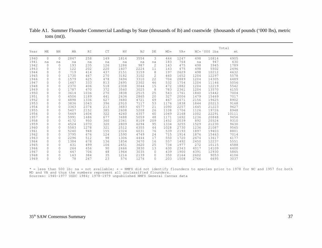
3735th SAW Consensus Summary
Table A1. Summer Flounder Commercial Landings by State (thousands of lb) and coastwide (thousands of pounds (‘000 lbs), metric tons (mt)).
TotalYear ME NH MA RI CT NY NJ DE MD+ VA+ NC+ '000 lbs mt 1940 0 0 2847 258 149 1814 3554 3 444 1247 498 10814 49051941 na na na na na na na na 183 764 na 947 4301942 0 0 193 235 126 1286 987 2 143 475 498 3945 17891943 0 0 122 202 220 1607 2224 11 143 475 498 5502 24961944 0 0 719 414 437 2151 3159 8 197 2629 498 10212 46321945 0 0 1730 467 270 3182 3102 2 460 1652 1204 12297 55781946 0 0 1579 625 478 3494 3310 22 704 2889 1204 14305 64891947 0 0 1467 333 813 2695 2302 46 532 1754 1204 11146 50561948 0 0 2370 406 518 2308 3044 15 472 1882 1204 12219 55421949 0 0 1787 470 372 3560 3025 8 783 2361 1204 13570 61551950 0 0 3614 1036 270 3838 2515 25 543 1761 1840 15442 70041951 0 0 4506 1189 441 2636 2865 20 327 2006 1479 15469 70171952 0 0 4898 1336 627 3680 4721 69 467 1671 2156 19625 89021953 0 0 3836 1043 396 2910 7117 53 1176 1838 1844 20213 91681954 0 0 3363 2374 213 3683 6577 21 1090 2257 1645 21223 96271955 0 0 5407 2152 385 2608 5208 26 1108 1706 1126 19726 89481956 0 0 5469 1604 322 4260 6357 60 1049 2168 1002 22291 101111957 0 0 5991 1486 677 3488 5059 48 1171 1692 1236 20848 94561958 0 0 4172 950 360 2341 8109 209 1452 2039 892 20524 93101959 0 0 4524 1070 320 2809 6294 95 1334 3255 1529 21230 96301960 0 0 5583 1278 321 2512 6355 44 1028 2730 1236 21087 95651961 0 0 5240 948 155 2324 6031 76 539 2193 1897 19403 88011962 0 0 3795 676 124 1590 4749 24 715 1914 1876 15463 70141963 0 0 2296 512 98 1306 4444 17 550 1720 2674 13617 61771964 0 0 1384 678 136 1854 3670 16 557 1492 2450 12237 55511965 0 0 431 499 106 2451 3620 25 734 1977 272 10115 45881966 0 0 264 456 90 2466 3830 13 630 2343 4017 14109 64001967 0 0 447 706 48 1964 3035 0 439 1900 4391 12930 58651968 0 0 163 384 35 1216 2139 0 350 2164 2602 9053 41061969 0 0 78 267 23 574 1276 0 203 1508 2766 6695 3037
* = less than 500 lb; na = not available; + = NMFS did not identify flounders to species prior to 1978 for NC and 1957 for bothMD and VA and thus the numbers represent all unclassified flounders. Sources: 1940-1977 USDC 1984; 1978-1979 unpublished NMFS General Canvas data
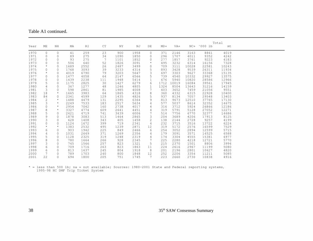
38 35th SAW Consensus Summary
Table A1 continued.
TotalYear ME NH MA RI CT NY NJ DE MD+ VA+ NC+ '000 lb mt 1970 0 0 41 259 23 900 1958 0 371 2146 3163 8861 40191971 0 0 89 275 34 1090 1850 0 296 1707 4011 9352 42421972 0 0 93 275 7 1101 1852 0 277 1857 3761 9223 41831973 0 0 506 640 52 1826 3091 * 495 3232 6314 16156 73281974 * 0 1689 2552 26 2487 3499 0 709 3111 10028 22581 102431975 0 0 1768 3093 39 3233 4314 5 893 3428 9539 26311 119341976 * 0 4019 6790 79 3203 5647 3 697 3303 9627 33368 151351977 0 0 1477 4058 64 2147 6566 5 739 4540 10332 29927 135751978 0 0 1439 2238 111 1948 5414 1 676 5940 10820 28586 129661979 5 0 1175 2825 30 1427 6279 6 1712 10019 16084 39561 179451980 4 0 367 1277 48 1246 4805 1 1324 8504 13643 31216 141591981 3 0 598 2861 81 1985 4008 7 403 3652 7459 21056 95511982 18 * 1665 3983 64 1865 4318 8 360 4332 6315 22928 104001983 84 0 2341 4599 129 1435 4826 5 937 8134 7057 29548 134031984 2 * 1488 4479 131 2295 6364 9 813 9673 12510 37765 171301985 3 * 2249 7533 183 2517 5634 4 577 5037 8614 32352 146751986 0 * 2954 7042 160 2738 4017 4 316 3712 5924 26866 121861987 8 * 3327 4774 609 2641 4451 4 319 5791 5128 27052 122711988 5 0 2421 4719 741 3439 6006 7 514 7756 6770 32377 146861989 9 0 1878 3083 513 1464 2865 3 204 3689 4206 17913 81251990 3 0 628 1408 343 405 1458 2 138 2144 2728 9257 41991991 0 0 1124 1672 399 719 2341 4 232 3715 3516 13722 62241992 * * 1383 2532 495 1239 2871 12 319 5172 2576 16599 75291993 6 0 903 1942 225 849 2466 6 254 3052 2894 12599 57151994 4 0 1031 2649 371 1269 2356 4 179 3091 3571 14525 65881995 5 0 1128 2325 319 1248 2319 4 174 3304 4555 15381 69771996 8 0 780 1664 266 928 2345 7 225 2280 4218 12721 57701997 3 0 745 1566 257 823 1321 5 215 2370 1501 8806 39941998 6 0 709 1716 263 823 1863 11 224 2616 2967 11199 50801999 6 0 813 1637 245 804 1918 8 201 2196 2801 10627 48202000 7 0 789 1703 240 800 1848 12 252 2206 3354 11211 50852001 22 0 694 1800 205 751 1745 7 223 2660 2730 10838 4916
* = less than 500 lb; na = not available; Sources: 1980-2001 State and Federal reporting systems, 1995-98 NC DMF Trip Ticket System
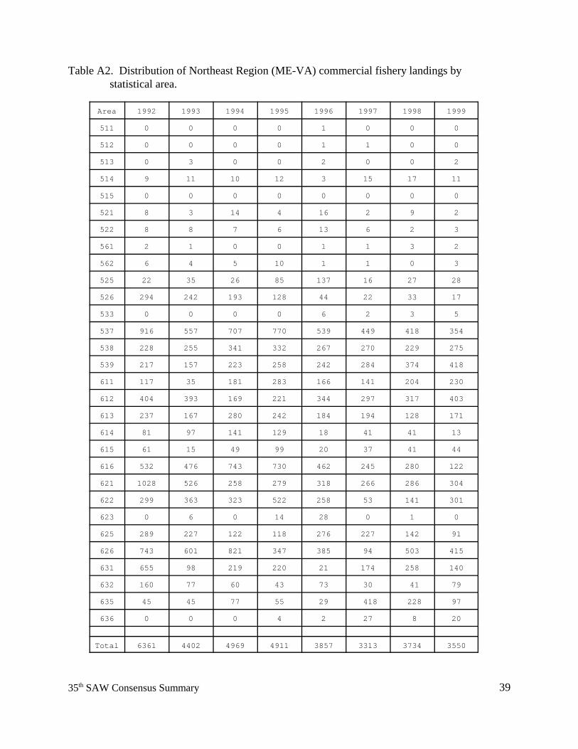
3935th SAW Consensus Summary
Table A2. Distribution of Northeast Region (ME-VA) commercial fishery landings by statistical area.
Area 1992 1993 1994 1995 1996 1997 1998 1999
511 0 0 0 0 1 0 0 0
512 0 0 0 0 1 1 0 0
513 0 3 0 0 2 0 0 2
514 9 11 10 12 3 15 17 11
515 0 0 0 0 0 0 0 0
521 8 3 14 4 16 2 9 2
522 8 8 7 6 13 6 2 3
561 2 1 0 0 1 1 3 2
562 6 4 5 10 1 1 0 3
525 22 35 26 85 137 16 27 28
526 294 242 193 128 44 22 33 17
533 0 0 0 0 6 2 3 5
537 916 557 707 770 539 449 418 354
538 228 255 341 332 267 270 229 275
539 217 157 223 258 242 284 374 418
611 117 35 181 283 166 141 204 230
612 404 393 169 221 344 297 317 403
613 237 167 280 242 184 194 128 171
614 81 97 141 129 18 41 41 13
615 61 15 49 99 20 37 41 44
616 532 476 743 730 462 245 280 122
621 1028 526 258 279 318 266 286 304
622 299 363 323 522 258 53 141 301
623 0 6 0 14 28 0 1 0
625 289 227 122 118 276 227 142 91
626 743 601 821 347 385 94 503 415
631 655 98 219 220 21 174 258 140
632 160 77 60 43 73 30 41 79
635 45 45 77 55 29 418 228 97
636 0 0 0 4 2 27 8 20
Total 6361 4402 4969 4911 3857 3313 3734 3550
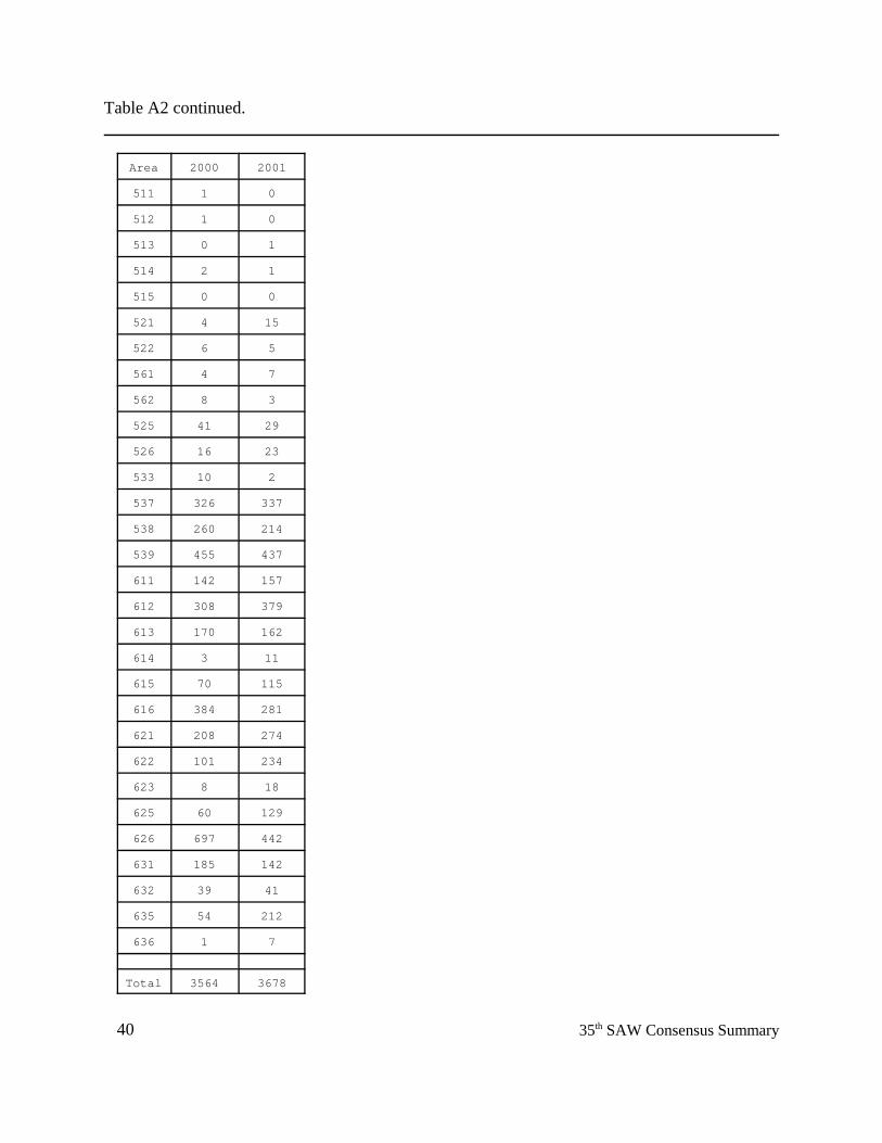
40 35th SAW Consensus Summary
Table A2 continued.
Area 2000 2001
511 1 0
512 1 0
513 0 1
514 2 1
515 0 0
521 4 15
522 6 5
561 4 7
562 8 3
525 41 29
526 16 23
533 10 2
537 326 337
538 260 214
539 455 437
611 142 157
612 308 379
613 170 162
614 3 11
615 70 115
616 384 281
621 208 274
622 101 234
623 8 18
625 60 129
626 697 442
631 185 142
632 39 41
635 54 212
636 1 7
Total 3564 3678
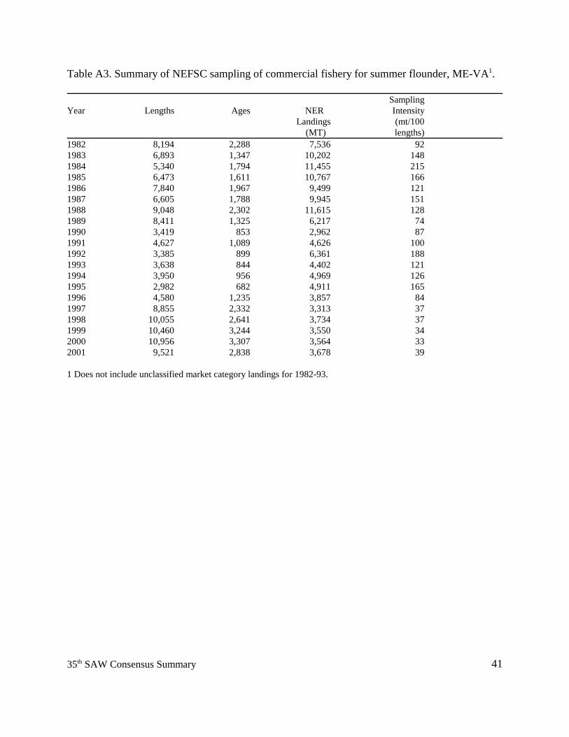
4135th SAW Consensus Summary
Table A3. Summary of NEFSC sampling of commercial fishery for summer flounder, ME-VA1.
SamplingYear Lengths Ages NER Intensity
Landings (mt/100(MT) lengths)
1982 8,194 2,288 7,536 921983 6,893 1,347 10,202 1481984 5,340 1,794 11,455 2151985 6,473 1,611 10,767 1661986 7,840 1,967 9,499 1211987 6,605 1,788 9,945 1511988 9,048 2,302 11,615 1281989 8,411 1,325 6,217 741990 3,419 853 2,962 871991 4,627 1,089 4,626 1001992 3,385 899 6,361 1881993 3,638 844 4,402 1211994 3,950 956 4,969 126 1995 2,982 682 4,911 1651996 4,580 1,235 3,857 841997 8,855 2,332 3,313 371998 10,055 2,641 3,734 371999 10,460 3,244 3,550 342000 10,956 3,307 3,564 332001 9,521 2,838 3,678 39
1 Does not include unclassified market category landings for 1982-93.
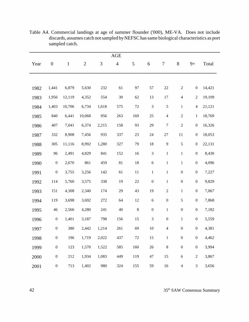
42 35th SAW Consensus Summary
Table A4. Commercial landings at age of summer flounder ('000), ME-VA. Does not includediscards, assumes catch not sampled by NEFSC has same biological characteristics as portsampled catch.
AGE
Year 0 1 2 3 4 5 6 7 8 9+ Total
1982 1,441 6,879 5,630 232 61 97 57 22 2 0 14,421
1983 1,956 12,119 4,352 554 30 62 13 17 4 2 19,109
1984 1,403 10,706 6,734 1,618 575 72 3 5 1 4 21,121
1985 840 6,441 10,068 956 263 169 25 4 2 1 18,769
1986 407 7,041 6,374 2,215 158 93 29 7 2 0 16,326
1987 332 8,908 7,456 935 337 23 24 27 11 0 18,053
1988 305 11,116 8,992 1,280 327 79 18 9 5 0 22,131
1989 96 2,491 4,829 841 152 16 3 1 1 0 8,430
1990 0 2,670 861 459 81 18 6 1 1 0 4,096
1991 0 3,755 3,256 142 61 11 1 1 0 0 7,227
1992 114 5,760 3,575 338 19 22 0 1 0 0 9,829
1993 151 4,308 2,340 174 29 43 19 2 1 0 7,067
1994 119 3,698 3,692 272 64 12 6 0 5 0 7,868
1995 46 2,566 4,280 241 40 8 0 1 0 0 7,182
1996 0 1,401 3,187 798 156 15 3 0 1 0 5,559
1997 0 380 2,442 1,214 261 69 10 4 0 0 4,381
1998 0 196 1,719 2,022 437 72 15 1 0 0 4,462
1999 0 123 1,570 1,522 585 160 26 8 0 0 3,994
2000 0 212 1,934 1,083 449 119 47 15 6 2 3,867
2001 0 713 1,402 980 324 155 59 16 4 3 3,656
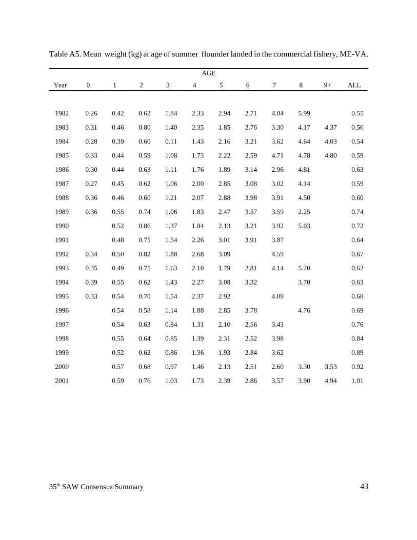
4335th SAW Consensus Summary
Table A5. Mean weight (kg) at age of summer flounder landed in the commercial fishery, ME-VA.
AGE
Year 0 1 2 3 4 5 6 7 8 9+ ALL
1982 0.26 0.42 0.62 1.84 2.33 2.94 2.71 4.04 5.99 0.55
1983 0.31 0.46 0.80 1.40 2.35 1.85 2.76 3.30 4.17 4.37 0.56
1984 0.28 0.39 0.60 0.11 1.43 2.16 3.21 3.62 4.64 4.03 0.54
1985 0.33 0.44 0.59 1.08 1.73 2.22 2.59 4.71 4.78 4.80 0.59
1986 0.30 0.44 0.63 1.11 1.76 1.89 3.14 2.96 4.81 0.63
1987 0.27 0.45 0.62 1.06 2.00 2.85 3.08 3.02 4.14 0.59
1988 0.36 0.46 0.60 1.21 2.07 2.88 3.98 3.91 4.50 0.60
1989 0.36 0.55 0.74 1.06 1.83 2.47 3.57 3.59 2.25 0.74
1990 0.52 0.86 1.37 1.84 2.13 3.21 3.92 5.03 0.72
1991 0.48 0.75 1.54 2.26 3.01 3.91 3.87 0.64
1992 0.34 0.50 0.82 1.88 2.68 3.09 4.59 0.67
1993 0.35 0.49 0.75 1.63 2.10 1.79 2.81 4.14 5.20 0.62
1994 0.39 0.55 0.62 1.43 2.27 3.08 3.32 3.70 0.63
1995 0.33 0.54 0.70 1.54 2.37 2.92 4.09 0.68
1996 0.54 0.58 1.14 1.88 2.85 3.78 4.76 0.69
1997 0.54 0.63 0.84 1.31 2.10 2.56 3.43 0.76
1998 0.55 0.64 0.85 1.39 2.31 2.52 3.98 0.84
1999 0.52 0.62 0.86 1.36 1.93 2.84 3.62 0.89
2000 0.57 0.68 0.97 1.46 2.13 2.51 2.60 3.30 3.53 0.92
2001 0.59 0.76 1.03 1.73 2.39 2.86 3.57 3.90 4.94 1.01
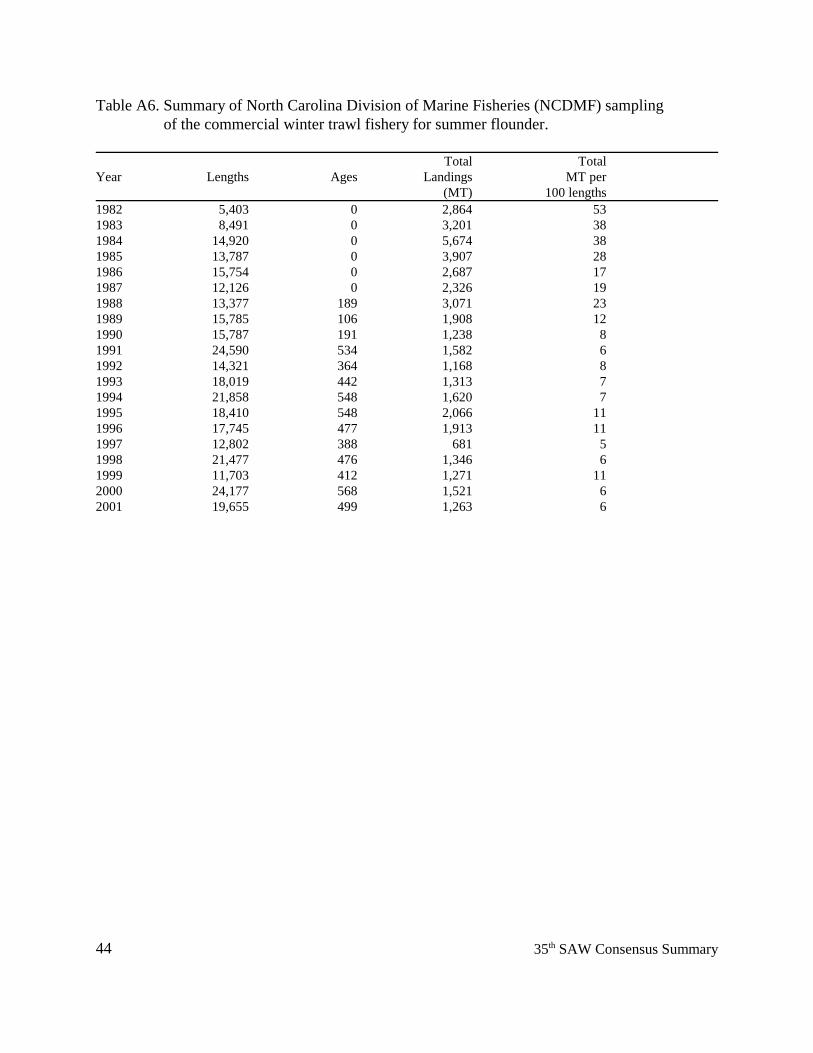
44 35th SAW Consensus Summary
Table A6. Summary of North Carolina Division of Marine Fisheries (NCDMF) sampling of the commercial winter trawl fishery for summer flounder.
Total TotalYear Lengths Ages Landings MT per
(MT) 100 lengths1982 5,403 0 2,864 531983 8,491 0 3,201 381984 14,920 0 5,674 381985 13,787 0 3,907 281986 15,754 0 2,687 171987 12,126 0 2,326 191988 13,377 189 3,071 231989 15,785 106 1,908 121990 15,787 191 1,238 81991 24,590 534 1,582 61992 14,321 364 1,168 81993 18,019 442 1,313 71994 21,858 548 1,620 71995 18,410 548 2,066 111996 17,745 477 1,913 111997 12,802 388 681 51998 21,477 476 1,346 61999 11,703 412 1,271 112000 24,177 568 1,521 62001 19,655 499 1,263 6
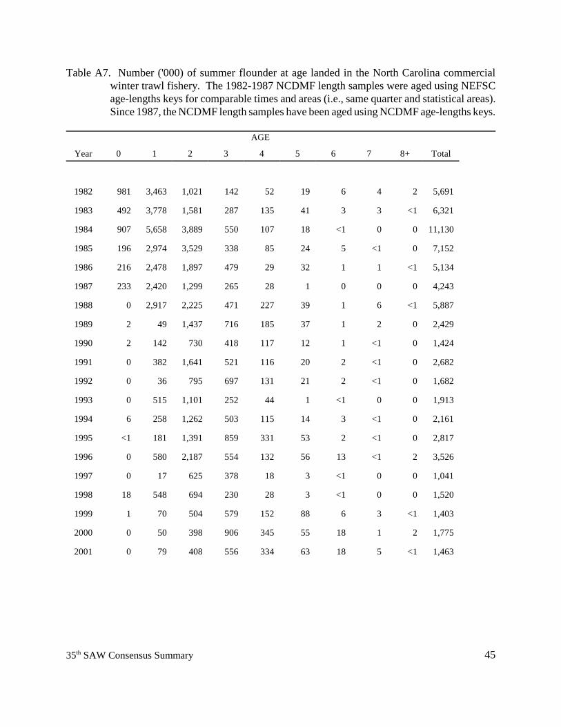
4535th SAW Consensus Summary
Table A7. Number ('000) of summer flounder at age landed in the North Carolina commercialwinter trawl fishery. The 1982-1987 NCDMF length samples were aged using NEFSCage-lengths keys for comparable times and areas (i.e., same quarter and statistical areas).Since 1987, the NCDMF length samples have been aged using NCDMF age-lengths keys.
AGE
Year 0 1 2 3 4 5 6 7 8+ Total
1982 981 3,463 1,021 142 52 19 6 4 2 5,691
1983 492 3,778 1,581 287 135 41 3 3 <1 6,321
1984 907 5,658 3,889 550 107 18 <1 0 0 11,130
1985 196 2,974 3,529 338 85 24 5 <1 0 7,152
1986 216 2,478 1,897 479 29 32 1 1 <1 5,134
1987 233 2,420 1,299 265 28 1 0 0 0 4,243
1988 0 2,917 2,225 471 227 39 1 6 <1 5,887
1989 2 49 1,437 716 185 37 1 2 0 2,429
1990 2 142 730 418 117 12 1 <1 0 1,424
1991 0 382 1,641 521 116 20 2 <1 0 2,682
1992 0 36 795 697 131 21 2 <1 0 1,682
1993 0 515 1,101 252 44 1 <1 0 0 1,913
1994 6 258 1,262 503 115 14 3 <1 0 2,161
1995 <1 181 1,391 859 331 53 2 <1 0 2,817
1996 0 580 2,187 554 132 56 13 <1 2 3,526
1997 0 17 625 378 18 3 <1 0 0 1,041
1998 18 548 694 230 28 3 <1 0 0 1,520
1999 1 70 504 579 152 88 6 3 <1 1,403
2000 0 50 398 906 345 55 18 1 2 1,775
2001 0 79 408 556 334 63 18 5 <1 1,463
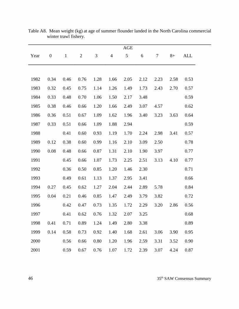
46 35th SAW Consensus Summary
Table A8. Mean weight (kg) at age of summer flounder landed in the North Carolina commercialwinter trawl fishery.
AGE
Year 0 1 2 3 4 5 6 7 8+ ALL
1982 0.34 0.46 0.76 1.28 1.66 2.05 2.12 2.23 2.58 0.53
1983 0.32 0.45 0.75 1.14 1.26 1.49 1.73 2.43 2.70 0.57
1984 0.33 0.48 0.70 1.06 1.50 2.17 3.48 0.59
1985 0.38 0.46 0.66 1.20 1.66 2.49 3.07 4.57 0.62
1986 0.36 0.51 0.67 1.09 1.62 1.96 3.40 3.23 3.63 0.64
1987 0.33 0.51 0.66 1.09 1.88 2.94 0.59
1988 0.41 0.60 0.93 1.19 1.70 2.24 2.98 3.41 0.57
1989 0.12 0.38 0.60 0.99 1.16 2.10 3.09 2.50 0.78
1990 0.08 0.48 0.66 0.87 1.31 2.10 1.90 3.97 0.77
1991 0.45 0.66 1.07 1.73 2.25 2.51 3.13 4.10 0.77
1992 0.36 0.50 0.85 1.20 1.46 2.30 0.71
1993 0.49 0.61 1.13 1.37 2.95 3.41 0.66
1994 0.27 0.45 0.62 1.27 2.04 2.44 2.89 5.78 0.84
1995 0.04 0.21 0.46 0.85 1.47 2.49 3.79 3.82 0.72
1996 0.42 0.47 0.73 1.35 1.72 2.29 3.20 2.86 0.56
1997 0.41 0.62 0.76 1.32 2.07 3.25 0.68
1998 0.41 0.71 0.89 1.24 1.49 2.80 3.38 0.89
1999 0.14 0.58 0.73 0.92 1.40 1.68 2.61 3.06 3.90 0.95
2000 0.56 0.66 0.80 1.20 1.96 2.59 3.31 3.52 0.90
2001 0.59 0.67 0.76 1.07 1.72 2.39 3.07 4.24 0.87
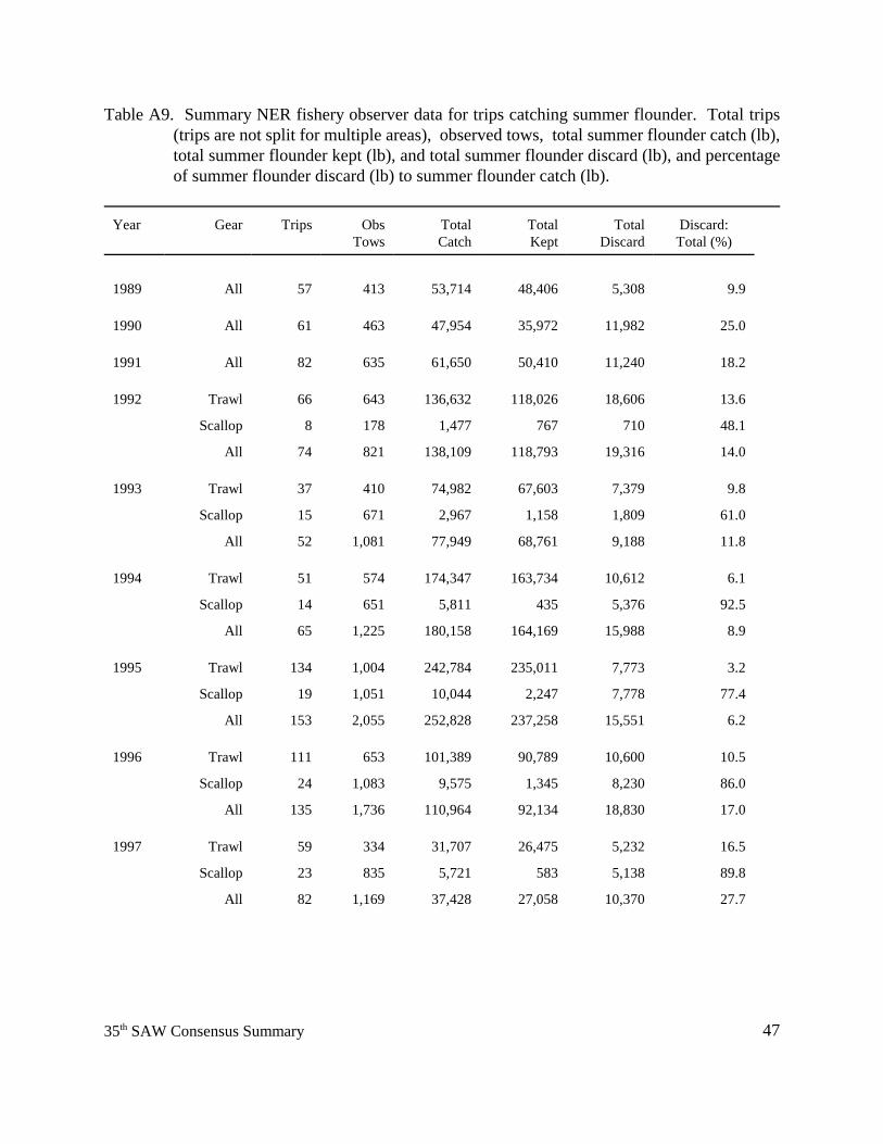
4735th SAW Consensus Summary
Table A9. Summary NER fishery observer data for trips catching summer flounder. Total trips(trips are not split for multiple areas), observed tows, total summer flounder catch (lb),total summer flounder kept (lb), and total summer flounder discard (lb), and percentageof summer flounder discard (lb) to summer flounder catch (lb).
Year Gear Trips ObsTows
TotalCatch
TotalKept
TotalDiscard
Discard:Total (%)
1989 All 57 413 53,714 48,406 5,308 9.9
1990 All 61 463 47,954 35,972 11,982 25.0
1991 All 82 635 61,650 50,410 11,240 18.2
1992 Trawl 66 643 136,632 118,026 18,606 13.6
Scallop 8 178 1,477 767 710 48.1
All 74 821 138,109 118,793 19,316 14.0
1993 Trawl 37 410 74,982 67,603 7,379 9.8
Scallop 15 671 2,967 1,158 1,809 61.0
All 52 1,081 77,949 68,761 9,188 11.8
1994 Trawl 51 574 174,347 163,734 10,612 6.1
Scallop 14 651 5,811 435 5,376 92.5
All 65 1,225 180,158 164,169 15,988 8.9
1995 Trawl 134 1,004 242,784 235,011 7,773 3.2
Scallop 19 1,051 10,044 2,247 7,778 77.4
All 153 2,055 252,828 237,258 15,551 6.2
1996 Trawl 111 653 101,389 90,789 10,600 10.5
Scallop 24 1,083 9,575 1,345 8,230 86.0
All 135 1,736 110,964 92,134 18,830 17.0
1997 Trawl 59 334 31,707 26,475 5,232 16.5
Scallop 23 835 5,721 583 5,138 89.8
All 82 1,169 37,428 27,058 10,370 27.7
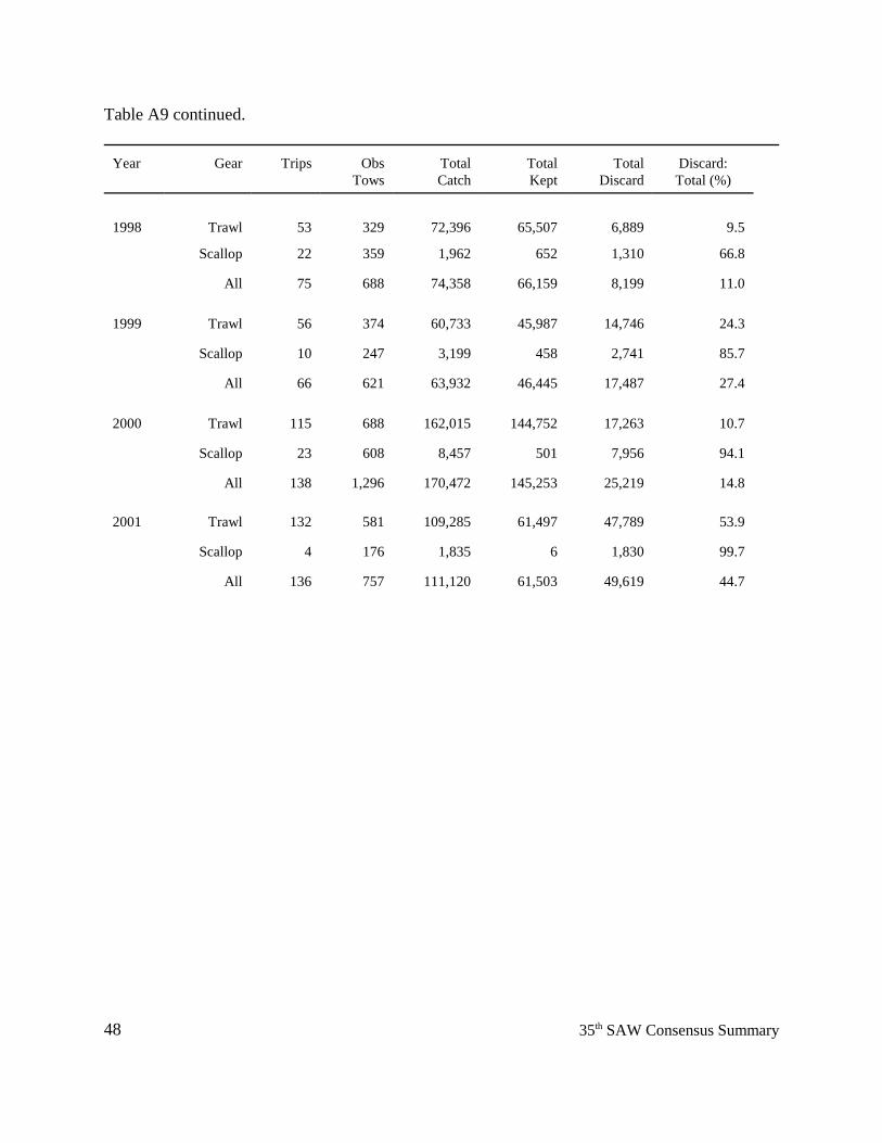
48 35th SAW Consensus Summary
Table A9 continued.
Year Gear Trips ObsTows
TotalCatch
TotalKept
TotalDiscard
Discard:Total (%)
1998 Trawl 53 329 72,396 65,507 6,889 9.5
Scallop 22 359 1,962 652 1,310 66.8
All 75 688 74,358 66,159 8,199 11.0
1999 Trawl 56 374 60,733 45,987 14,746 24.3
Scallop 10 247 3,199 458 2,741 85.7
All 66 621 63,932 46,445 17,487 27.4
2000 Trawl 115 688 162,015 144,752 17,263 10.7
Scallop 23 608 8,457 501 7,956 94.1
All 138 1,296 170,472 145,253 25,219 14.8
2001 Trawl 132 581 109,285 61,497 47,789 53.9
Scallop 4 176 1,835 6 1,830 99.7
All 136 757 111,120 61,503 49,619 44.7
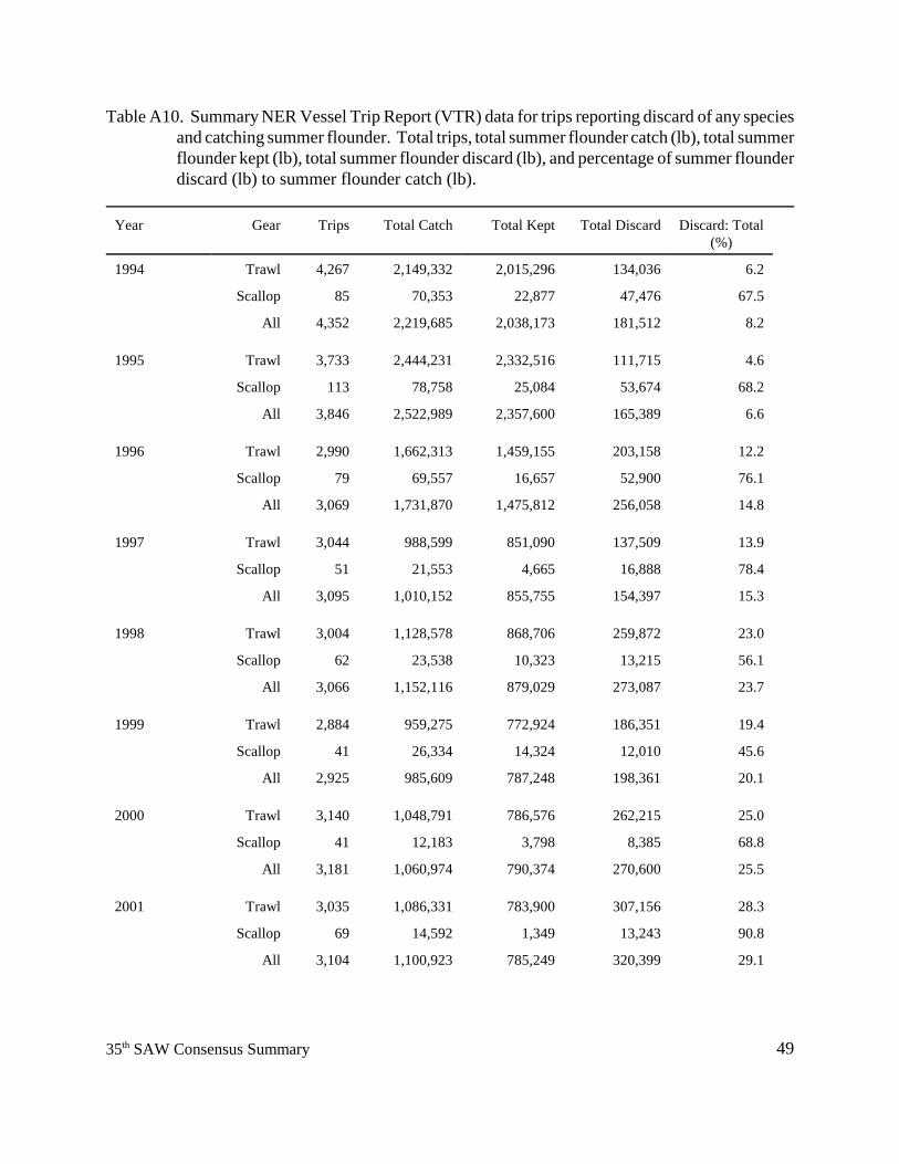
4935th SAW Consensus Summary
Table A10. Summary NER Vessel Trip Report (VTR) data for trips reporting discard of any speciesand catching summer flounder. Total trips, total summer flounder catch (lb), total summerflounder kept (lb), total summer flounder discard (lb), and percentage of summer flounderdiscard (lb) to summer flounder catch (lb).
Year Gear Trips Total Catch Total Kept Total Discard Discard: Total(%)
1994 Trawl 4,267 2,149,332 2,015,296 134,036 6.2
Scallop 85 70,353 22,877 47,476 67.5
All 4,352 2,219,685 2,038,173 181,512 8.2
1995 Trawl 3,733 2,444,231 2,332,516 111,715 4.6
Scallop 113 78,758 25,084 53,674 68.2
All 3,846 2,522,989 2,357,600 165,389 6.6
1996 Trawl 2,990 1,662,313 1,459,155 203,158 12.2
Scallop 79 69,557 16,657 52,900 76.1
All 3,069 1,731,870 1,475,812 256,058 14.8
1997 Trawl 3,044 988,599 851,090 137,509 13.9
Scallop 51 21,553 4,665 16,888 78.4
All 3,095 1,010,152 855,755 154,397 15.3
1998 Trawl 3,004 1,128,578 868,706 259,872 23.0
Scallop 62 23,538 10,323 13,215 56.1
All 3,066 1,152,116 879,029 273,087 23.7
1999 Trawl 2,884 959,275 772,924 186,351 19.4
Scallop 41 26,334 14,324 12,010 45.6
All 2,925 985,609 787,248 198,361 20.1
2000 Trawl 3,140 1,048,791 786,576 262,215 25.0
Scallop 41 12,183 3,798 8,385 68.8
All 3,181 1,060,974 790,374 270,600 25.5
2001 Trawl 3,035 1,086,331 783,900 307,156 28.3
Scallop 69 14,592 1,349 13,243 90.8
All 3,104 1,100,923 785,249 320,399 29.1
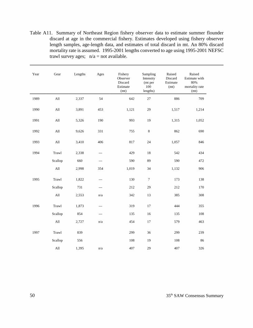
50 35th SAW Consensus Summary
Table A11. Summary of Northeast Region fishery observer data to estimate summer flounderdiscard at age in the commercial fishery. Estimates developed using fishery observerlength samples, age-length data, and estimates of total discard in mt. An 80% discardmortality rate is assumed. 1995-2001 lengths converted to age using 1995-2001 NEFSCtrawl survey ages; n/a = not available.
Year Gear Lengths Ages FisheryObserverDiscardEstimate
(mt)
SamplingIntensity(mt per
100 lengths)
RaisedDiscardEstimate
(mt)
RaisedEstimate with
80%mortality rate
(mt)
1989 All 2,337 54 642 27 886 709
1990 All 3,891 453 1,121 29 1,517 1,214
1991 All 5,326 190 993 19 1,315 1,052
1992 All 9,626 331 755 8 862 690
1993 All 3,410 406 817 24 1,057 846
1994 Trawl 2,338 --- 429 18 542 434
Scallop 660 --- 590 89 590 472
All 2,998 354 1,019 34 1,132 906
1995 Trawl 1,822 --- 130 7 173 138
Scallop 731 --- 212 29 212 170
All 2,553 n/a 342 13 385 308
1996 Trawl 1,873 --- 319 17 444 355
Scallop 854 --- 135 16 135 108
All 2,727 n/a 454 17 579 463
1997 Trawl 839 299 36 299 239
Scallop 556 108 19 108 86
All 1,395 n/a 407 29 407 326
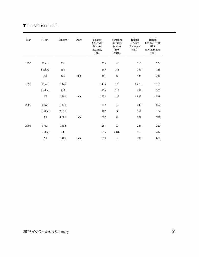
5135th SAW Consensus Summary
Table A11 continued.
Year Gear Lengths Ages FisheryObserverDiscardEstimate
(mt)
SamplingIntensity(mt per
100 lengths)
RaisedDiscardEstimate
(mt)
RaisedEstimate with
80%mortality rate
(mt)
1998 Trawl 721 318 44 318 254
Scallop 150 169 113 169 135
All 871 n/a 487 56 487 389
1999 Trawl 1,145 1,476 129 1,476 1,181
Scallop 216 459 213 459 367
All 1,361 n/a 1,935 142 1,935 1,548
2000 Trawl 1,470 740 50 740 592
Scallop 2,611 167 6 167 134
All 4,081 n/a 907 22 907 726
2001 Trawl 1,394 284 20 284 227
Scallop 11 515 4,682 515 412
All 1,405 n/a 799 57 799 639
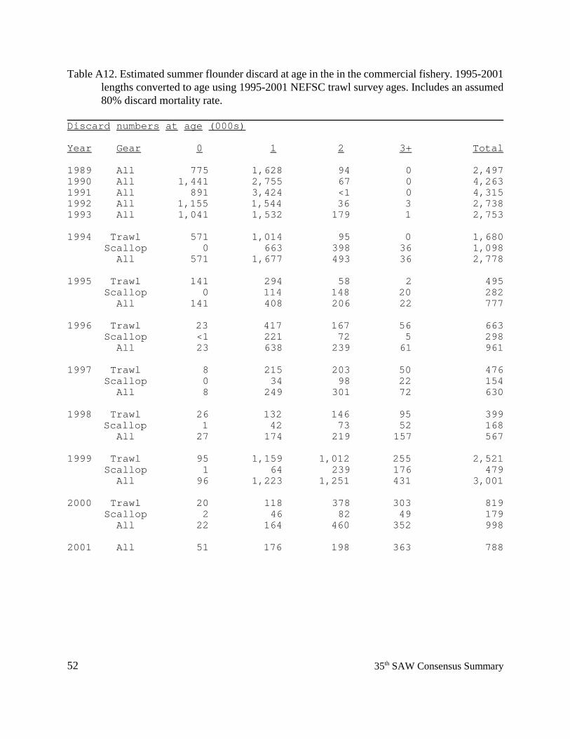
52 35th SAW Consensus Summary
Table A12. Estimated summer flounder discard at age in the in the commercial fishery. 1995-2001lengths converted to age using 1995-2001 NEFSC trawl survey ages. Includes an assumed80% discard mortality rate.
Discard numbers at age (000s)
Year Gear 0 1 2 3+ Total
1989 All 775 1,628 94 0 2,4971990 All 1,441 2,755 67 0 4,2631991 All 891 3,424 <1 0 4,3151992 All 1,155 1,544 36 3 2,7381993 All 1,041 1,532 179 1 2,753
1994 Trawl 571 1,014 95 0 1,680 Scallop 0 663 398 36 1,098 All 571 1,677 493 36 2,778
1995 Trawl 141 294 58 2 495 Scallop 0 114 148 20 282 All 141 408 206 22 777
1996 Trawl 23 417 167 56 663 Scallop <1 221 72 5 298 All 23 638 239 61 961
1997 Trawl 8 215 203 50 476 Scallop 0 34 98 22 154 All 8 249 301 72 630
1998 Trawl 26 132 146 95 399 Scallop 1 42 73 52 168 All 27 174 219 157 567
1999 Trawl 95 1,159 1,012 255 2,521 Scallop 1 64 239 176 479 All 96 1,223 1,251 431 3,001
2000 Trawl 20 118 378 303 819 Scallop 2 46 82 49 179 All 22 164 460 352 998
2001 All 51 176 198 363 788
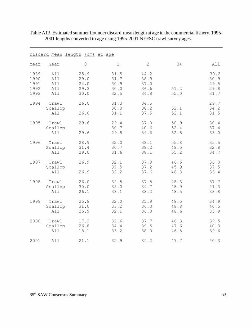
5335th SAW Consensus Summary
Table A13. Estimated summer flounder discard mean length at age in the commercial fishery. 1995-2001 lengths converted to age using 1995-2001 NEFSC trawl survey ages.
Discard mean length (cm) at age
Year Gear 0 1 2 3+ All
1989 All 25.9 31.5 44.2 30.2 1990 All 29.0 31.7 38.9 30.91991 All 24.0 30.9 37.0 29.51992 All 29.3 30.0 36.6 51.2 29.81993 All 30.0 32.5 34.8 55.0 31.7
1994 Trawl 26.0 31.3 34.5 29.7 Scallop 30.8 38.2 52.1 34.2 All 26.0 31.1 37.5 52.1 31.5
1995 Trawl 29.6 29.4 37.0 50.9 30.4 Scallop 30.7 40.6 52.4 37.4 All 29.6 29.8 39.6 52.5 33.0
1996 Trawl 28.9 32.0 38.1 55.8 35.5 Scallop 31.4 30.7 38.2 48.5 32.8 All 29.0 31.6 38.1 55.2 34.7
1997 Trawl 26.9 32.1 37.8 46.6 36.0 Scallop 32.5 37.2 45.9 37.5 All 26.9 32.2 37.6 46.3 36.4
1998 Trawl 26.0 32.5 37.5 48.3 37.7 Scallop 30.0 35.0 39.7 48.9 41.3 All 26.1 33.1 38.2 48.5 38.8
1999 Trawl 25.8 32.0 35.9 48.5 34.9 Scallop 31.0 33.2 36.3 48.8 40.5 All 25.9 32.1 36.0 48.6 35.9
2000 Trawl 17.2 32.6 37.7 46.3 39.5 Scallop 26.8 34.4 39.5 47.6 40.3 All 18.1 33.2 38.0 46.5 39.6
2001 All 21.1 32.9 39.2 47.7 40.3
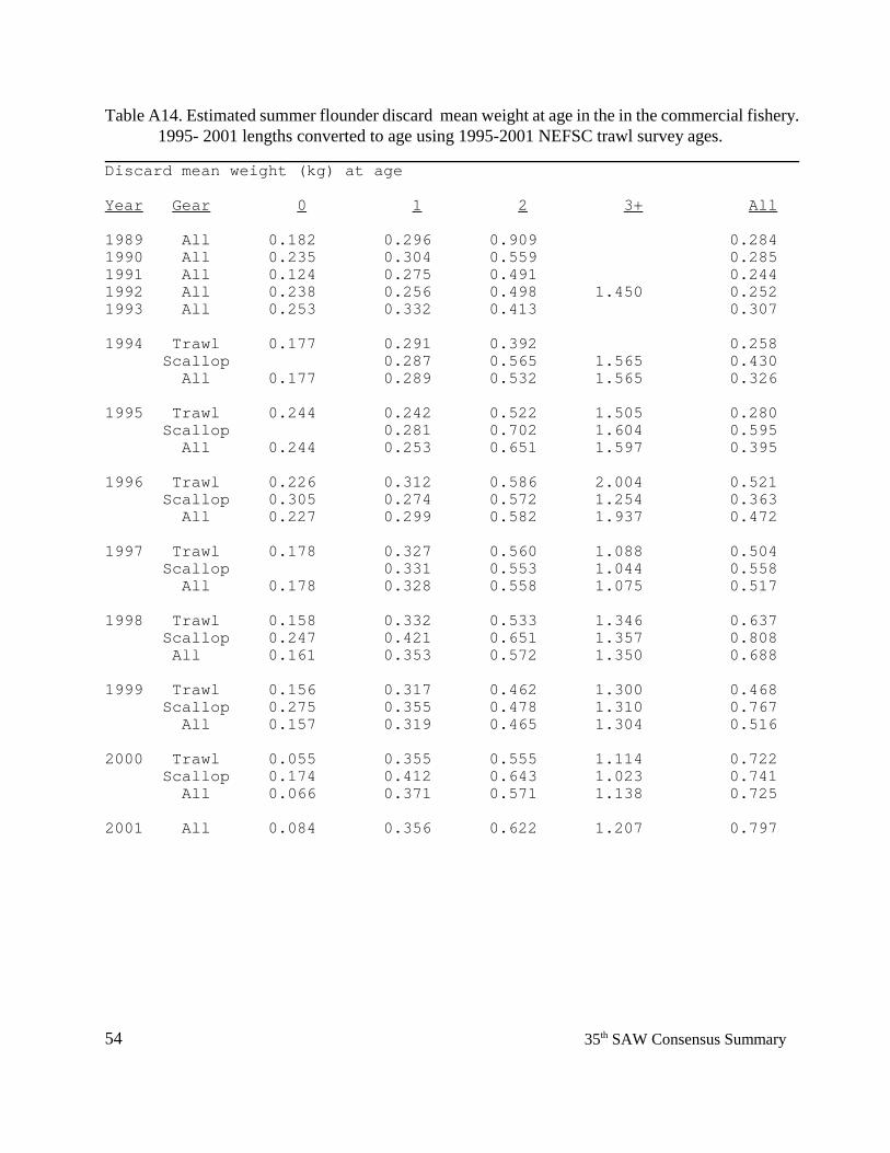
54 35th SAW Consensus Summary
Table A14. Estimated summer flounder discard mean weight at age in the in the commercial fishery.1995- 2001 lengths converted to age using 1995-2001 NEFSC trawl survey ages.
Discard mean weight (kg) at age
Year Gear 0 1 2 3+ All
1989 All 0.182 0.296 0.909 0.2841990 All 0.235 0.304 0.559 0.2851991 All 0.124 0.275 0.491 0.2441992 All 0.238 0.256 0.498 1.450 0.2521993 All 0.253 0.332 0.413 0.307
1994 Trawl 0.177 0.291 0.392 0.258 Scallop 0.287 0.565 1.565 0.430 All 0.177 0.289 0.532 1.565 0.326
1995 Trawl 0.244 0.242 0.522 1.505 0.280 Scallop 0.281 0.702 1.604 0.595 All 0.244 0.253 0.651 1.597 0.395
1996 Trawl 0.226 0.312 0.586 2.004 0.521 Scallop 0.305 0.274 0.572 1.254 0.363 All 0.227 0.299 0.582 1.937 0.472
1997 Trawl 0.178 0.327 0.560 1.088 0.504 Scallop 0.331 0.553 1.044 0.558 All 0.178 0.328 0.558 1.075 0.517
1998 Trawl 0.158 0.332 0.533 1.346 0.637 Scallop 0.247 0.421 0.651 1.357 0.808 All 0.161 0.353 0.572 1.350 0.688
1999 Trawl 0.156 0.317 0.462 1.300 0.468 Scallop 0.275 0.355 0.478 1.310 0.767 All 0.157 0.319 0.465 1.304 0.516
2000 Trawl 0.055 0.355 0.555 1.114 0.722 Scallop 0.174 0.412 0.643 1.023 0.741 All 0.066 0.371 0.571 1.138 0.725
2001 All 0.084 0.356 0.622 1.207 0.797
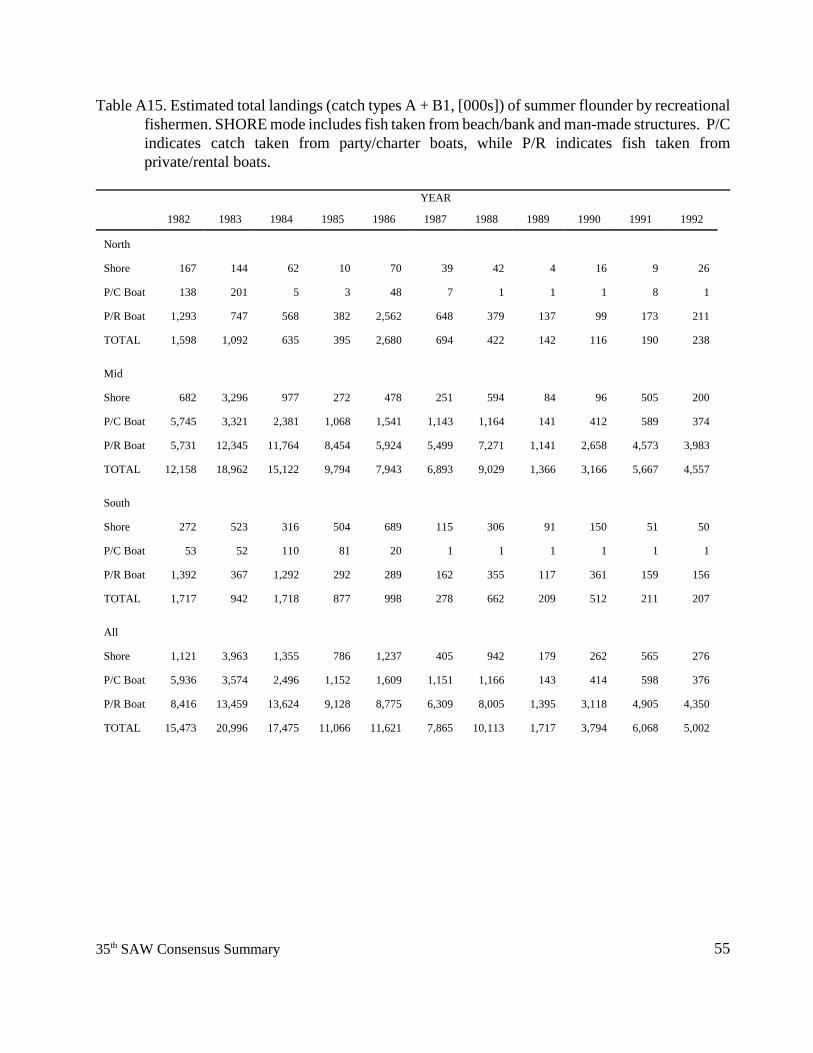
5535th SAW Consensus Summary
Table A15. Estimated total landings (catch types A + B1, [000s]) of summer flounder by recreationalfishermen. SHORE mode includes fish taken from beach/bank and man-made structures. P/Cindicates catch taken from party/charter boats, while P/R indicates fish taken fromprivate/rental boats.
YEAR
1982 1983 1984 1985 1986 1987 1988 1989 1990 1991 1992
North
Shore 167 144 62 10 70 39 42 4 16 9 26
P/C Boat 138 201 5 3 48 7 1 1 1 8 1
P/R Boat 1,293 747 568 382 2,562 648 379 137 99 173 211
TOTAL 1,598 1,092 635 395 2,680 694 422 142 116 190 238
Mid
Shore 682 3,296 977 272 478 251 594 84 96 505 200
P/C Boat 5,745 3,321 2,381 1,068 1,541 1,143 1,164 141 412 589 374
P/R Boat 5,731 12,345 11,764 8,454 5,924 5,499 7,271 1,141 2,658 4,573 3,983
TOTAL 12,158 18,962 15,122 9,794 7,943 6,893 9,029 1,366 3,166 5,667 4,557
South
Shore 272 523 316 504 689 115 306 91 150 51 50
P/C Boat 53 52 110 81 20 1 1 1 1 1 1
P/R Boat 1,392 367 1,292 292 289 162 355 117 361 159 156
TOTAL 1,717 942 1,718 877 998 278 662 209 512 211 207
All
Shore 1,121 3,963 1,355 786 1,237 405 942 179 262 565 276
P/C Boat 5,936 3,574 2,496 1,152 1,609 1,151 1,166 143 414 598 376
P/R Boat 8,416 13,459 13,624 9,128 8,775 6,309 8,005 1,395 3,118 4,905 4,350
TOTAL 15,473 20,996 17,475 11,066 11,621 7,865 10,113 1,717 3,794 6,068 5,002
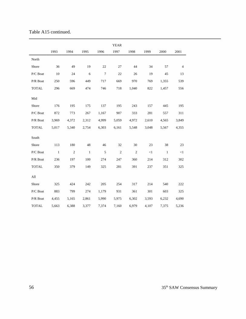
56 35th SAW Consensus Summary
Table A15 continued.
YEAR
1993 1994 1995 1996 1997 1998 1999 2000 2001
North
Shore 36 49 19 22 27 44 34 57 4
P/C Boat 10 24 6 7 22 26 19 45 13
P/R Boat 250 596 449 717 669 970 769 1,355 539
TOTAL 296 669 474 746 718 1,040 822 1,457 556
Mid
Shore 176 195 175 137 195 243 157 445 195
P/C Boat 872 773 267 1,167 907 333 281 557 311
P/R Boat 3,969 4,372 2,312 4,999 5,059 4,972 2,610 4,565 3,849
TOTAL 5,017 5,340 2,754 6,303 6,161 5,548 3,048 5,567 4,355
South
Shore 113 180 48 46 32 30 23 38 23
P/C Boat 1 2 1 5 2 2 <1 1 <1
P/R Boat 236 197 100 274 247 360 214 312 302
TOTAL 350 379 149 325 281 391 237 351 325
All
Shore 325 424 242 205 254 317 214 540 222
P/C Boat 883 799 274 1,179 931 361 301 603 325
P/R Boat 4,455 5,165 2,861 5,990 5,975 6,302 3,593 6,232 4,690
TOTAL 5,663 6,388 3,377 7,374 7,160 6,979 4,107 7,375 5,236
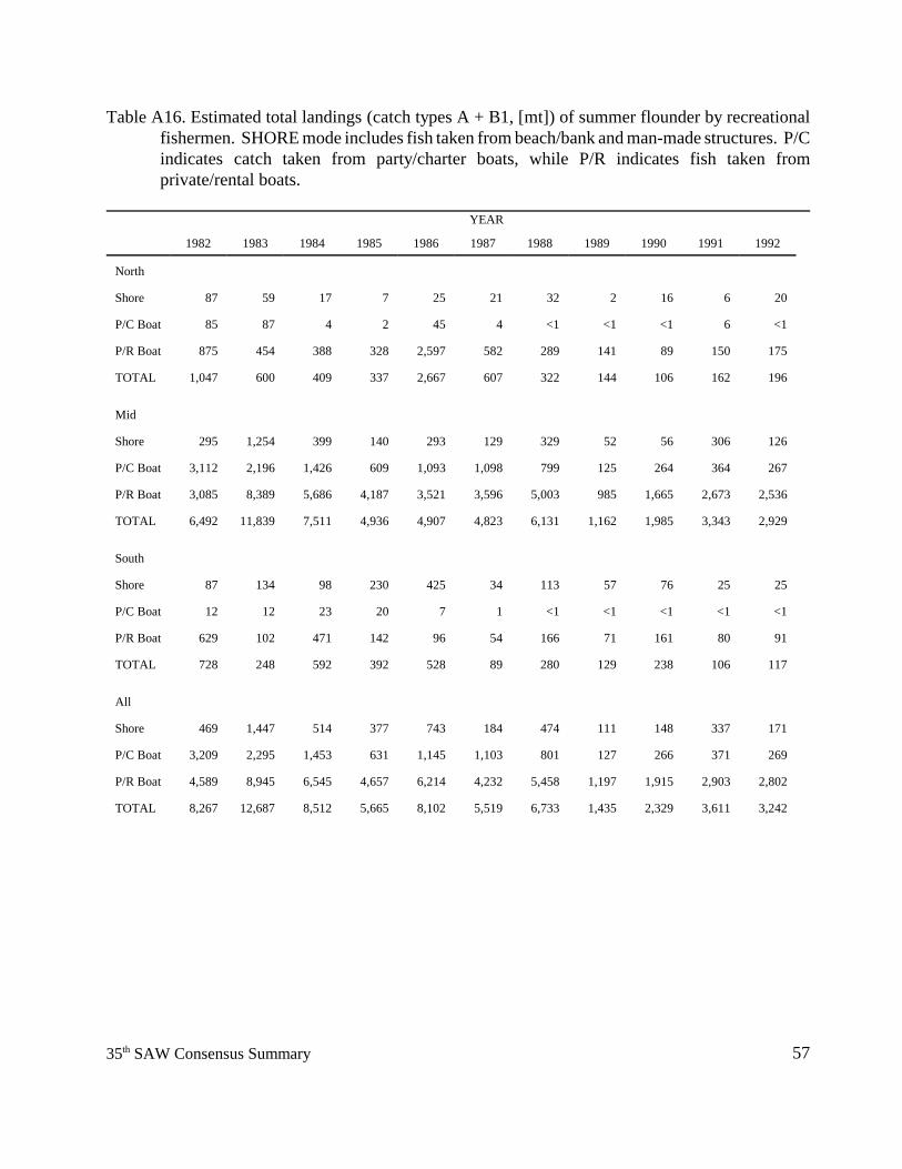
5735th SAW Consensus Summary
Table A16. Estimated total landings (catch types A + B1, [mt]) of summer flounder by recreationalfishermen. SHORE mode includes fish taken from beach/bank and man-made structures. P/Cindicates catch taken from party/charter boats, while P/R indicates fish taken fromprivate/rental boats.
YEAR
1982 1983 1984 1985 1986 1987 1988 1989 1990 1991 1992
North
Shore 87 59 17 7 25 21 32 2 16 6 20
P/C Boat 85 87 4 2 45 4 <1 <1 <1 6 <1
P/R Boat 875 454 388 328 2,597 582 289 141 89 150 175
TOTAL 1,047 600 409 337 2,667 607 322 144 106 162 196
Mid
Shore 295 1,254 399 140 293 129 329 52 56 306 126
P/C Boat 3,112 2,196 1,426 609 1,093 1,098 799 125 264 364 267
P/R Boat 3,085 8,389 5,686 4,187 3,521 3,596 5,003 985 1,665 2,673 2,536
TOTAL 6,492 11,839 7,511 4,936 4,907 4,823 6,131 1,162 1,985 3,343 2,929
South
Shore 87 134 98 230 425 34 113 57 76 25 25
P/C Boat 12 12 23 20 7 1 <1 <1 <1 <1 <1
P/R Boat 629 102 471 142 96 54 166 71 161 80 91
TOTAL 728 248 592 392 528 89 280 129 238 106 117
All
Shore 469 1,447 514 377 743 184 474 111 148 337 171
P/C Boat 3,209 2,295 1,453 631 1,145 1,103 801 127 266 371 269
P/R Boat 4,589 8,945 6,545 4,657 6,214 4,232 5,458 1,197 1,915 2,903 2,802
TOTAL 8,267 12,687 8,512 5,665 8,102 5,519 6,733 1,435 2,329 3,611 3,242
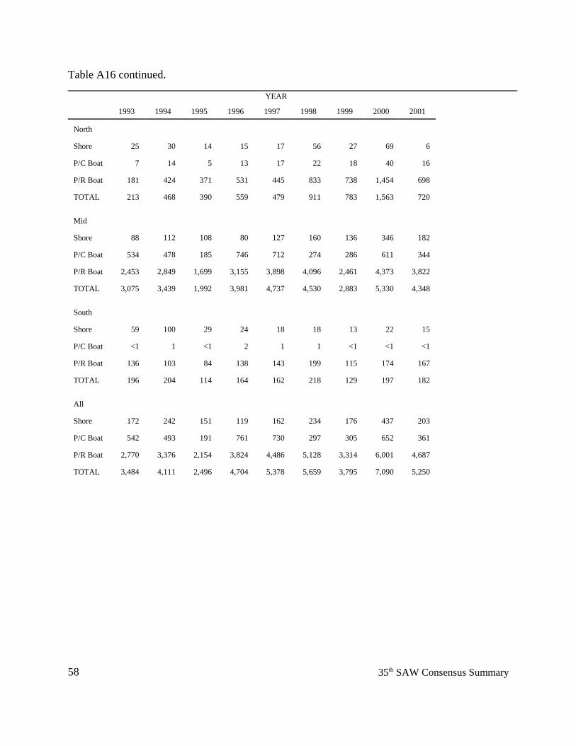
58 35th SAW Consensus Summary
Table A16 continued.
YEAR
1993 1994 1995 1996 1997 1998 1999 2000 2001
North
Shore 25 30 14 15 17 56 27 69 6
P/C Boat 7 14 5 13 17 22 18 40 16
P/R Boat 181 424 371 531 445 833 738 1,454 698
TOTAL 213 468 390 559 479 911 783 1,563 720
Mid
Shore 88 112 108 80 127 160 136 346 182
P/C Boat 534 478 185 746 712 274 286 611 344
P/R Boat 2,453 2,849 1,699 3,155 3,898 4,096 2,461 4,373 3,822
TOTAL 3,075 3,439 1,992 3,981 4,737 4,530 2,883 5,330 4,348
South
Shore 59 100 29 24 18 18 13 22 15
P/C Boat <1 1 <1 2 1 1 <1 <1 <1
P/R Boat 136 103 84 138 143 199 115 174 167
TOTAL 196 204 114 164 162 218 129 197 182
All
Shore 172 242 151 119 162 234 176 437 203
P/C Boat 542 493 191 761 730 297 305 652 361
P/R Boat 2,770 3,376 2,154 3,824 4,486 5,128 3,314 6,001 4,687
TOTAL 3,484 4,111 2,496 4,704 5,378 5,659 3,795 7,090 5,250
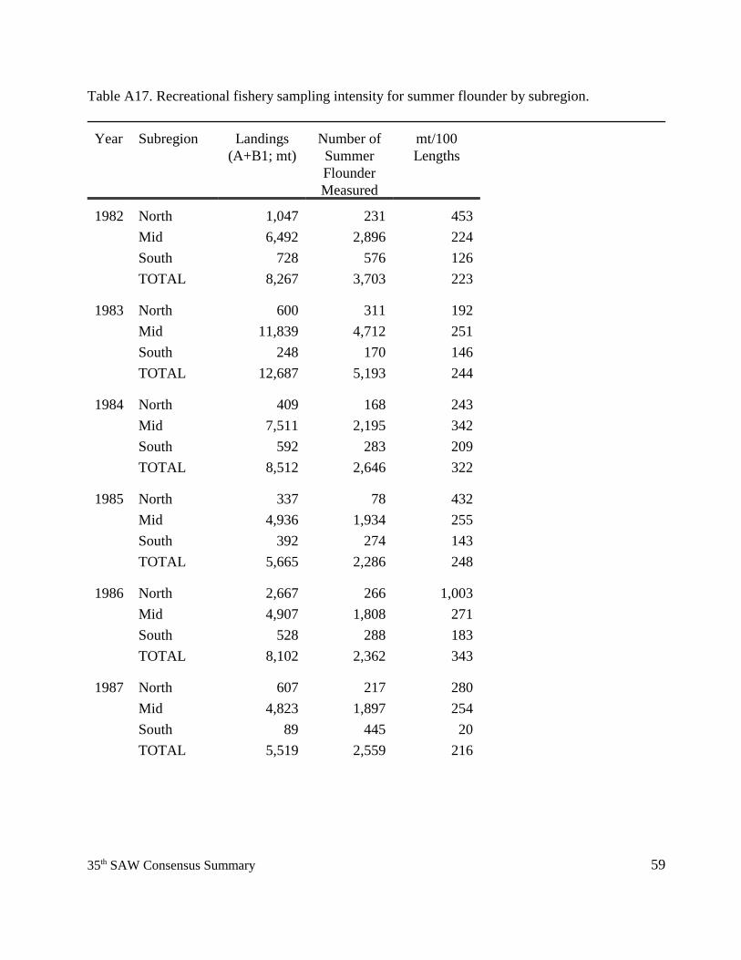
5935th SAW Consensus Summary
Table A17. Recreational fishery sampling intensity for summer flounder by subregion.
Year Subregion Landings(A+B1; mt)
Number ofSummerFlounderMeasured
mt/100Lengths
1982 North 1,047 231 453Mid 6,492 2,896 224South 728 576 126TOTAL 8,267 3,703 223
1983 North 600 311 192Mid 11,839 4,712 251South 248 170 146TOTAL 12,687 5,193 244
1984 North 409 168 243Mid 7,511 2,195 342South 592 283 209TOTAL 8,512 2,646 322
1985 North 337 78 432Mid 4,936 1,934 255South 392 274 143TOTAL 5,665 2,286 248
1986 North 2,667 266 1,003Mid 4,907 1,808 271South 528 288 183TOTAL 8,102 2,362 343
1987 North 607 217 280Mid 4,823 1,897 254South 89 445 20TOTAL 5,519 2,559 216
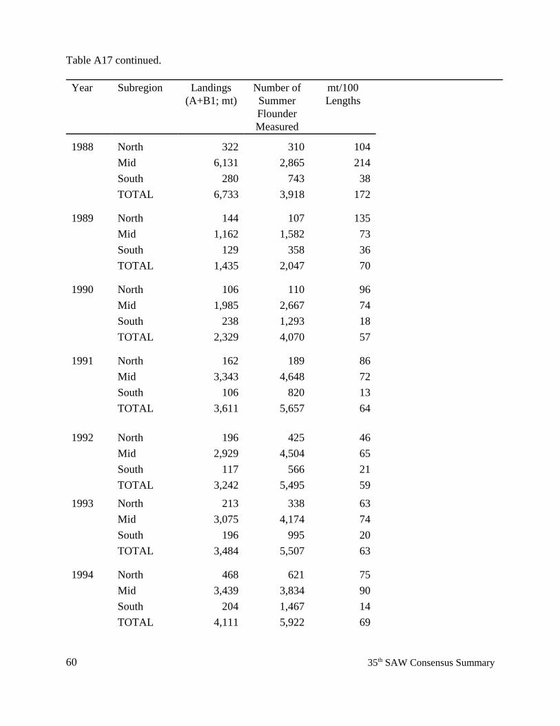
60 35th SAW Consensus Summary
Table A17 continued.
Year Subregion Landings(A+B1; mt)
Number ofSummerFlounderMeasured
mt/100Lengths
1988 North 322 310 104Mid 6,131 2,865 214South 280 743 38TOTAL 6,733 3,918 172
1989 North 144 107 135Mid 1,162 1,582 73South 129 358 36TOTAL 1,435 2,047 70
1990 North 106 110 96Mid 1,985 2,667 74South 238 1,293 18TOTAL 2,329 4,070 57
1991 North 162 189 86Mid 3,343 4,648 72South 106 820 13TOTAL 3,611 5,657 64
1992 North 196 425 46Mid 2,929 4,504 65South 117 566 21TOTAL 3,242 5,495 59
1993 North 213 338 63Mid 3,075 4,174 74South 196 995 20TOTAL 3,484 5,507 63
1994 North 468 621 75Mid 3,439 3,834 90South 204 1,467 14TOTAL 4,111 5,922 69
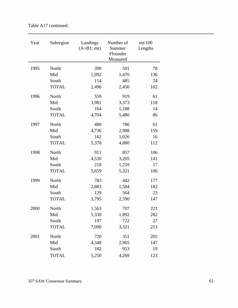
6135th SAW Consensus Summary
Table A17 continued.
Year Subregion Landings(A+B1; mt)
Number ofSummerFlounderMeasured
mt/100Lengths
1995 North 390 501 78Mid 1,992 1,470 136South 114 485 24TOTAL 2,496 2,456 102
1996 North 559 919 61Mid 3,981 3,373 118South 164 1,188 14TOTAL 4,704 5,480 86
1997 North 480 786 61Mid 4,736 2,988 159South 162 1,026 16TOTAL 5,378 4,800 112
1998 North 911 857 106Mid 4,530 3,205 141South 218 1,259 17TOTAL 5,659 5,321 106
1999 North 783 442 177Mid 2,883 1,584 182South 129 564 23TOTAL 3,795 2,590 147
2000 North 1,563 707 221Mid 5,330 1,892 282South 197 722 27TOTAL 7,090 3,321 213
2001 North 720 351 205Mid 4,348 2,965 147South 182 953 19TOTAL 5,250 4,269 123
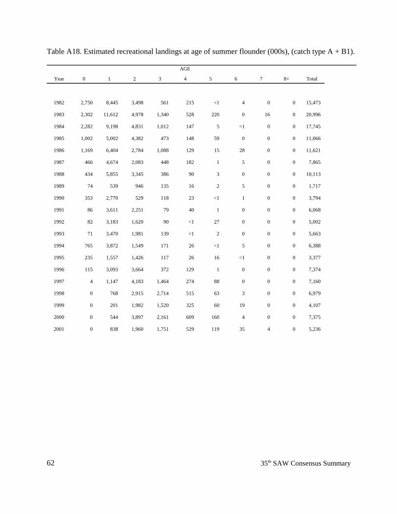
62 35th SAW Consensus Summary
Table A18. Estimated recreational landings at age of summer flounder (000s), (catch type A + B1).
AGE
Year 0 1 2 3 4 5 6 7 8+ Total
1982 2,750 8,445 3,498 561 215 <1 4 0 0 15,473
1983 2,302 11,612 4,978 1,340 528 220 0 16 0 20,996
1984 2,282 9,198 4,831 1,012 147 5 <1 0 0 17,745
1985 1,002 5,002 4,382 473 148 59 0 0 0 11,066
1986 1,169 6,404 2,784 1,088 129 15 28 0 0 11,621
1987 466 4,674 2,083 448 182 1 5 0 0 7,865
1988 434 5,855 3,345 386 90 3 0 0 0 10,113
1989 74 539 946 135 16 2 5 0 0 1,717
1990 353 2,770 529 118 23 <1 1 0 0 3,794
1991 86 3,611 2,251 79 40 1 0 0 0 6,068
1992 82 3,183 1,620 90 <1 27 0 0 0 5,002
1993 71 3,470 1,981 139 <1 2 0 0 0 5,663
1994 765 3,872 1,549 171 26 <1 5 0 0 6,388
1995 235 1,557 1,426 117 26 16 <1 0 0 3,377
1996 115 3,093 3,664 372 129 1 0 0 0 7,374
1997 4 1,147 4,183 1,464 274 88 0 0 0 7,160
1998 0 768 2,915 2,714 515 63 3 0 0 6,979
1999 0 201 1,982 1,520 325 60 19 0 0 4,107
2000 0 544 3,897 2,161 609 160 4 0 0 7,375
2001 0 838 1,960 1,751 529 119 35 4 0 5,236
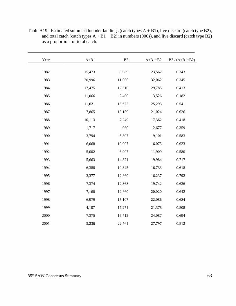
6335th SAW Consensus Summary
Table A19. Estimated summer flounder landings (catch types A + B1), live discard (catch type B2),and total catch (catch types A + B1 + B2) in numbers (000s), and live discard (catch type B2)as a proportion of total catch.
Year A+B1 B2 A+B1+B2 B2 / (A+B1+B2)
1982 15,473 8,089 23,562 0.343
1983 20,996 11,066 32,062 0.345
1984 17,475 12,310 29,785 0.413
1985 11,066 2,460 13,526 0.182
1986 11,621 13,672 25,293 0.541
1987 7,865 13,159 21,024 0.626
1988 10,113 7,249 17,362 0.418
1989 1,717 960 2,677 0.359
1990 3,794 5,307 9,101 0.583
1991 6,068 10,007 16,075 0.623
1992 5,002 6,907 11,909 0.580
1993 5,663 14,321 19,984 0.717
1994 6,388 10,345 16,733 0.618
1995 3,377 12,860 16,237 0.792
1996 7,374 12,368 19,742 0.626
1997 7,160 12,860 20,020 0.642
1998 6,979 15,107 22,086 0.684
1999 4,107 17,271 21,378 0.808
2000 7,375 16,712 24,087 0.694
2001 5,236 22,561 27,797 0.812
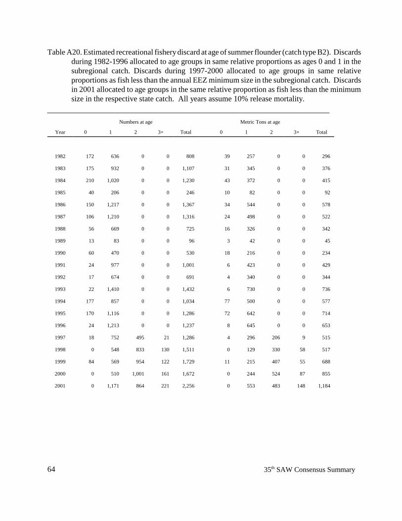
64 35th SAW Consensus Summary
Table A20. Estimated recreational fishery discard at age of summer flounder (catch type B2). Discardsduring 1982-1996 allocated to age groups in same relative proportions as ages 0 and 1 in thesubregional catch. Discards during 1997-2000 allocated to age groups in same relativeproportions as fish less than the annual EEZ minimum size in the subregional catch. Discardsin 2001 allocated to age groups in the same relative proportion as fish less than the minimumsize in the respective state catch. All years assume 10% release mortality.
Numbers at age Metric Tons at age
Year 0 1 2 3+ Total 0 1 2 3+ Total
1982 172 636 0 0 808 39 257 0 0 296
1983 175 932 0 0 1,107 31 345 0 0 376
1984 210 1,020 0 0 1,230 43 372 0 0 415
1985 40 206 0 0 246 10 82 0 0 92
1986 150 1,217 0 0 1,367 34 544 0 0 578
1987 106 1,210 0 0 1,316 24 498 0 0 522
1988 56 669 0 0 725 16 326 0 0 342
1989 13 83 0 0 96 3 42 0 0 45
1990 60 470 0 0 530 18 216 0 0 234
1991 24 977 0 0 1,001 6 423 0 0 429
1992 17 674 0 0 691 4 340 0 0 344
1993 22 1,410 0 0 1,432 6 730 0 0 736
1994 177 857 0 0 1,034 77 500 0 0 577
1995 170 1,116 0 0 1,286 72 642 0 0 714
1996 24 1,213 0 0 1,237 8 645 0 0 653
1997 18 752 495 21 1,286 4 296 206 9 515
1998 0 548 833 130 1,511 0 129 330 58 517
1999 84 569 954 122 1,729 11 215 407 55 688
2000 0 510 1,001 161 1,672 0 244 524 87 855
2001 0 1,171 864 221 2,256 0 553 483 148 1,184
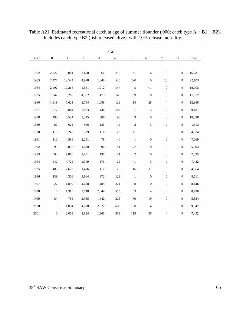
6535th SAW Consensus Summary
Table A21. Estimated recreational catch at age of summer flounder ('000; catch type A + B1 + B2).Includes catch type B2 (fish released alive) with 10% release mortality.
AGE
Year 0 1 2 3 4 5 6 7 8+ Total
1982 2,922 9,081 3,498 561 215 <1 4 0 0 16,281
1983 2,477 12,544 4,978 1,340 528 220 0 16 0 22,103
1984 2,492 10,218 4,831 1,012 147 5 <1 0 0 18,705
1985 1,042 5,208 4,382 473 148 59 0 0 0 11,312
1986 1,319 7,621 2,784 1,088 129 15 28 4 0 12,988
1987 572 5,884 2,083 448 182 1 5 6 0 9,181
1988 490 6,524 3,345 386 90 3 0 0 0 10,838
1989 87 622 946 135 16 2 5 0 0 1,813
1990 413 3,240 529 118 23 <1 1 0 0 4,324
1991 110 4,588 2,251 79 40 1 0 0 0 7,069
1992 99 3,857 1,620 90 <1 27 0 0 0 5,693
1993 93 4,880 1,981 139 <1 2 0 0 0 7,095
1994 942 4,729 1,549 171 26 <1 5 0 0 7,422
1995 405 2,673 1,426 117 26 16 <1 0 0 4,664
1996 139 4,306 3,664 372 129 1 0 0 0 8,611
1997 22 1,899 4,678 1,485 274 88 0 0 0 8,446
1998 0 1,316 3,748 2,844 515 63 4 0 0 8,490
1999 84 769 2,935 1,642 325 60 19 0 0 5,834
2000 0 1,054 4,898 2,322 609 160 4 0 0 9,047
2001 0 2,009 2,824 1,963 538 119 35 4 0 7,492
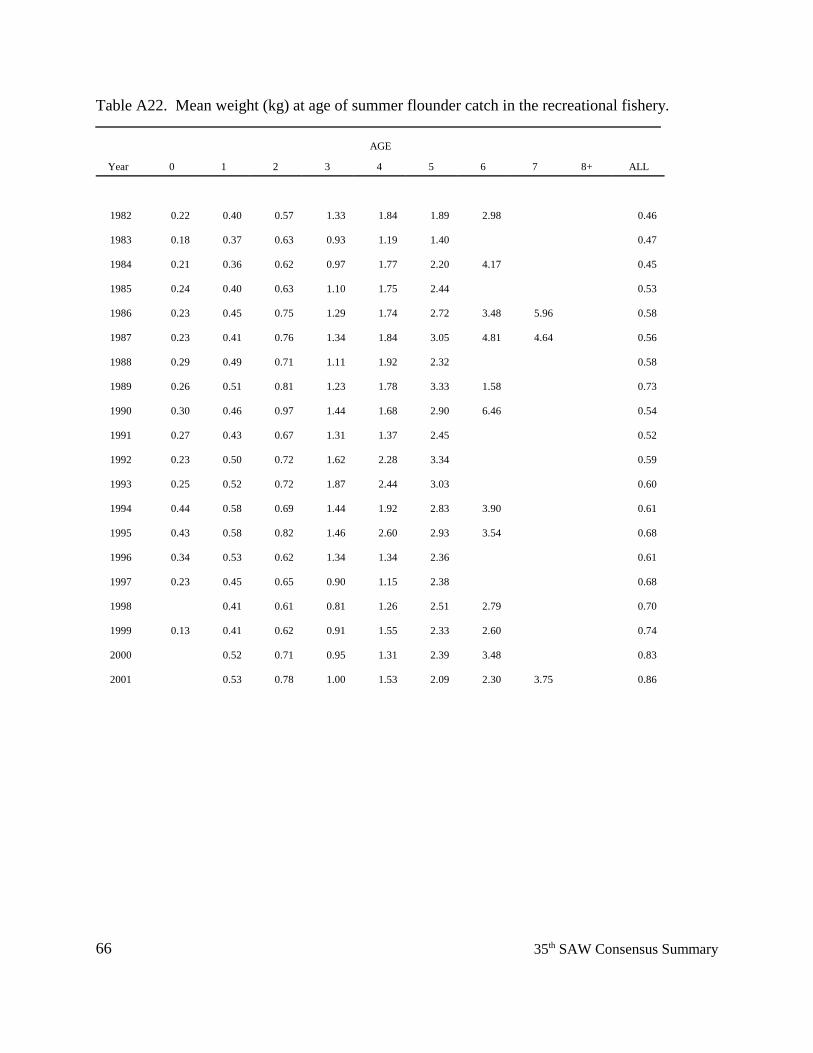
66 35th SAW Consensus Summary
Table A22. Mean weight (kg) at age of summer flounder catch in the recreational fishery.
AGE
Year 0 1 2 3 4 5 6 7 8+ ALL
1982 0.22 0.40 0.57 1.33 1.84 1.89 2.98 0.46
1983 0.18 0.37 0.63 0.93 1.19 1.40 0.47
1984 0.21 0.36 0.62 0.97 1.77 2.20 4.17 0.45
1985 0.24 0.40 0.63 1.10 1.75 2.44 0.53
1986 0.23 0.45 0.75 1.29 1.74 2.72 3.48 5.96 0.58
1987 0.23 0.41 0.76 1.34 1.84 3.05 4.81 4.64 0.56
1988 0.29 0.49 0.71 1.11 1.92 2.32 0.58
1989 0.26 0.51 0.81 1.23 1.78 3.33 1.58 0.73
1990 0.30 0.46 0.97 1.44 1.68 2.90 6.46 0.54
1991 0.27 0.43 0.67 1.31 1.37 2.45 0.52
1992 0.23 0.50 0.72 1.62 2.28 3.34 0.59
1993 0.25 0.52 0.72 1.87 2.44 3.03 0.60
1994 0.44 0.58 0.69 1.44 1.92 2.83 3.90 0.61
1995 0.43 0.58 0.82 1.46 2.60 2.93 3.54 0.68
1996 0.34 0.53 0.62 1.34 1.34 2.36 0.61
1997 0.23 0.45 0.65 0.90 1.15 2.38 0.68
1998 0.41 0.61 0.81 1.26 2.51 2.79 0.70
1999 0.13 0.41 0.62 0.91 1.55 2.33 2.60 0.74
2000 0.52 0.71 0.95 1.31 2.39 3.48 0.83
2001 0.53 0.78 1.00 1.53 2.09 2.30 3.75 0.86
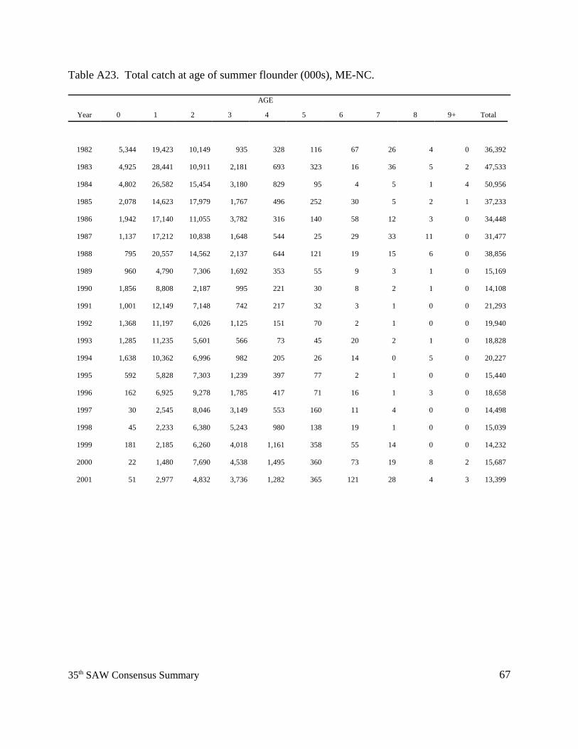
6735th SAW Consensus Summary
Table A23. Total catch at age of summer flounder (000s), ME-NC.
AGE
Year 0 1 2 3 4 5 6 7 8 9+ Total
1982 5,344 19,423 10,149 935 328 116 67 26 4 0 36,392
1983 4,925 28,441 10,911 2,181 693 323 16 36 5 2 47,533
1984 4,802 26,582 15,454 3,180 829 95 4 5 1 4 50,956
1985 2,078 14,623 17,979 1,767 496 252 30 5 2 1 37,233
1986 1,942 17,140 11,055 3,782 316 140 58 12 3 0 34,448
1987 1,137 17,212 10,838 1,648 544 25 29 33 11 0 31,477
1988 795 20,557 14,562 2,137 644 121 19 15 6 0 38,856
1989 960 4,790 7,306 1,692 353 55 9 3 1 0 15,169
1990 1,856 8,808 2,187 995 221 30 8 2 1 0 14,108
1991 1,001 12,149 7,148 742 217 32 3 1 0 0 21,293
1992 1,368 11,197 6,026 1,125 151 70 2 1 0 0 19,940
1993 1,285 11,235 5,601 566 73 45 20 2 1 0 18,828
1994 1,638 10,362 6,996 982 205 26 14 0 5 0 20,227
1995 592 5,828 7,303 1,239 397 77 2 1 0 0 15,440
1996 162 6,925 9,278 1,785 417 71 16 1 3 0 18,658
1997 30 2,545 8,046 3,149 553 160 11 4 0 0 14,498
1998 45 2,233 6,380 5,243 980 138 19 1 0 0 15,039
1999 181 2,185 6,260 4,018 1,161 358 55 14 0 0 14,232
2000 22 1,480 7,690 4,538 1,495 360 73 19 8 2 15,687
2001 51 2,977 4,832 3,736 1,282 365 121 28 4 3 13,399
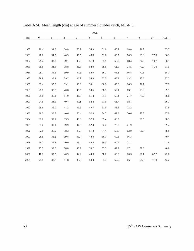
68 35th SAW Consensus Summary
Table A24. Mean length (cm) at age of summer flounder catch, ME-NC.
AGE
Year 0 1 2 3 4 5 6 7 8 9+ ALL
1982 29.4 34.5 38.8 50.7 55.3 61.0 60.7 68.0 71.2 35.7
1983 28.8 34.5 40.9 46.5 48.8 51.6 60.7 60.9 69.3 72.0 36.3
1984 29.4 33.8 39.1 45.9 51.3 57.9 66.8 68.4 74.0 70.7 36.1
1985 30.6 34.8 38.8 46.8 53.9 58.6 61.5 74.5 73.3 75.0 37.5
1986 29.7 35.6 39.9 47.5 54.0 56.2 65.8 66.4 72.8 38.2
1987 29.9 35.3 39.7 46.9 55.8 63.3 65.9 63.2 73.5 37.7
1988 32.4 35.8 39.1 46.6 53.1 60.2 69.6 68.5 72.7 37.9
1989 27.1 35.7 40.8 45.5 50.6 58.5 59.1 63.1 59.0 39.1
1990 29.6 35.1 41.9 46.8 51.4 57.4 66.4 71.7 75.2 36.6
1991 24.8 34.5 40.4 47.1 54.3 61.0 61.7 68.1 36.7
1992 29.6 36.0 41.2 46.9 49.7 61.0 58.8 72.2 37.9
1993 30.3 36.5 40.6 50.4 52.9 54.7 62.6 70.6 75.5 37.9
1994 32.2 37.1 39.3 49.6 57.3 63.4 66.3 68.5 38.3
1995 33.7 37.1 39.9 44.9 52.4 62.2 70.5 71.9 39.4
1996 32.6 36.9 38.3 45.7 51.3 54.4 58.5 63.0 66.0 38.8
1997 28.5 36.2 39.8 43.4 48.3 58.1 60.8 66.3 40.4
1998 28.7 37.2 40.0 43.4 49.5 59.3 60.9 71.1 41.6
1999 25.3 33.6 38.8 43.9 50.7 55.5 62.2 67.1 67.0 40.8
2000 18.1 37.2 40.9 44.2 49.3 58.0 60.8 60.3 66.1 67.7 42.8
2001 21.1 37.7 41.8 45.0 50.4 57.3 60.5 66.1 68.9 71.8 43.2
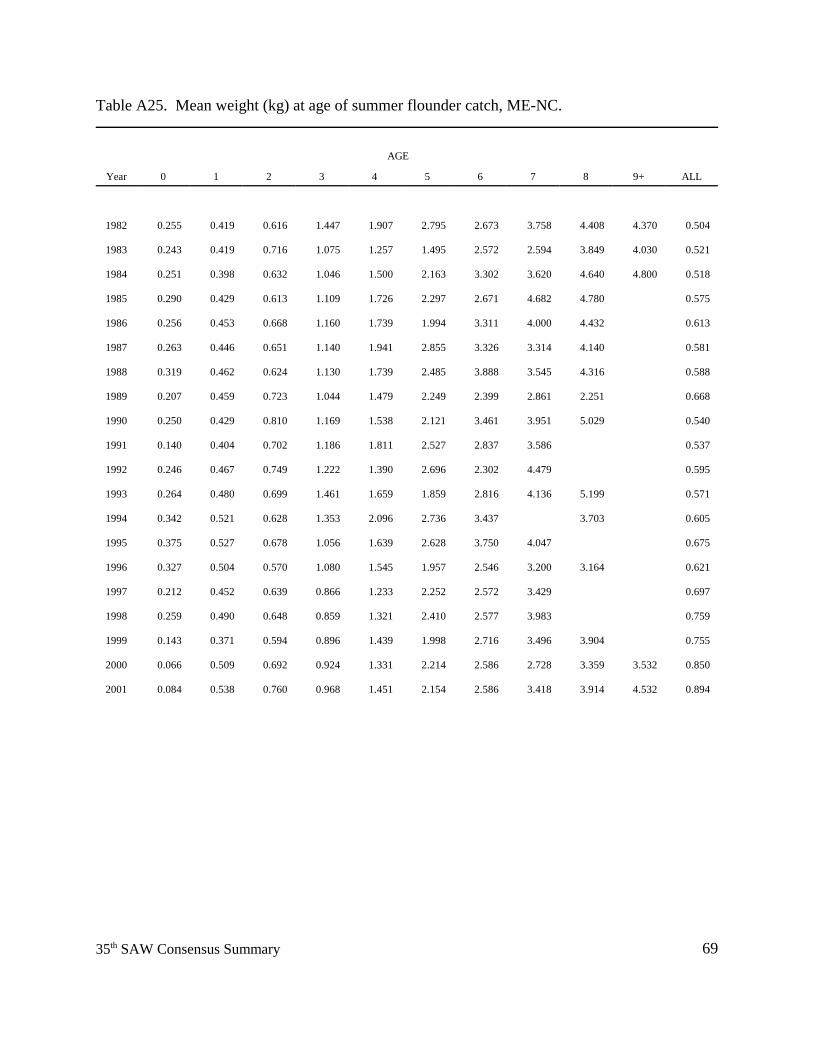
6935th SAW Consensus Summary
Table A25. Mean weight (kg) at age of summer flounder catch, ME-NC.
AGE
Year 0 1 2 3 4 5 6 7 8 9+ ALL
1982 0.255 0.419 0.616 1.447 1.907 2.795 2.673 3.758 4.408 4.370 0.504
1983 0.243 0.419 0.716 1.075 1.257 1.495 2.572 2.594 3.849 4.030 0.521
1984 0.251 0.398 0.632 1.046 1.500 2.163 3.302 3.620 4.640 4.800 0.518
1985 0.290 0.429 0.613 1.109 1.726 2.297 2.671 4.682 4.780 0.575
1986 0.256 0.453 0.668 1.160 1.739 1.994 3.311 4.000 4.432 0.613
1987 0.263 0.446 0.651 1.140 1.941 2.855 3.326 3.314 4.140 0.581
1988 0.319 0.462 0.624 1.130 1.739 2.485 3.888 3.545 4.316 0.588
1989 0.207 0.459 0.723 1.044 1.479 2.249 2.399 2.861 2.251 0.668
1990 0.250 0.429 0.810 1.169 1.538 2.121 3.461 3.951 5.029 0.540
1991 0.140 0.404 0.702 1.186 1.811 2.527 2.837 3.586 0.537
1992 0.246 0.467 0.749 1.222 1.390 2.696 2.302 4.479 0.595
1993 0.264 0.480 0.699 1.461 1.659 1.859 2.816 4.136 5.199 0.571
1994 0.342 0.521 0.628 1.353 2.096 2.736 3.437 3.703 0.605
1995 0.375 0.527 0.678 1.056 1.639 2.628 3.750 4.047 0.675
1996 0.327 0.504 0.570 1.080 1.545 1.957 2.546 3.200 3.164 0.621
1997 0.212 0.452 0.639 0.866 1.233 2.252 2.572 3.429 0.697
1998 0.259 0.490 0.648 0.859 1.321 2.410 2.577 3.983 0.759
1999 0.143 0.371 0.594 0.896 1.439 1.998 2.716 3.496 3.904 0.755
2000 0.066 0.509 0.692 0.924 1.331 2.214 2.586 2.728 3.359 3.532 0.850
2001 0.084 0.538 0.760 0.968 1.451 2.154 2.586 3.418 3.914 4.532 0.894
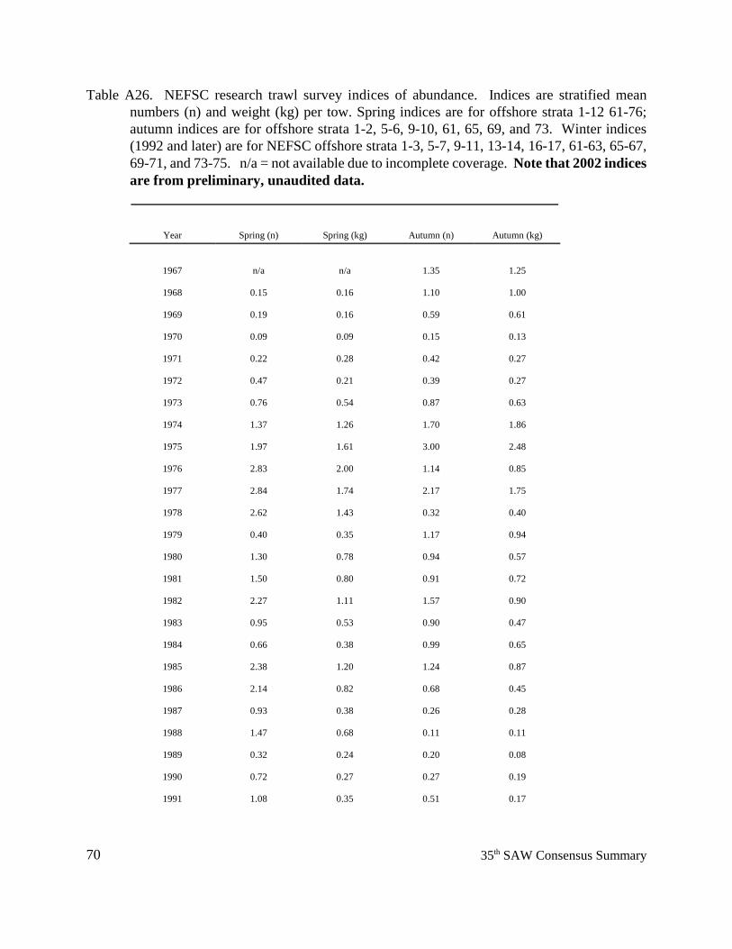
70 35th SAW Consensus Summary
Table A26. NEFSC research trawl survey indices of abundance. Indices are stratified meannumbers (n) and weight (kg) per tow. Spring indices are for offshore strata 1-12 61-76;autumn indices are for offshore strata 1-2, 5-6, 9-10, 61, 65, 69, and 73. Winter indices(1992 and later) are for NEFSC offshore strata 1-3, 5-7, 9-11, 13-14, 16-17, 61-63, 65-67,69-71, and 73-75. n/a = not available due to incomplete coverage. Note that 2002 indicesare from preliminary, unaudited data.
Year Spring (n) Spring (kg) Autumn (n) Autumn (kg)
1967 n/a n/a 1.35 1.25
1968 0.15 0.16 1.10 1.00
1969 0.19 0.16 0.59 0.61
1970 0.09 0.09 0.15 0.13
1971 0.22 0.28 0.42 0.27
1972 0.47 0.21 0.39 0.27
1973 0.76 0.54 0.87 0.63
1974 1.37 1.26 1.70 1.86
1975 1.97 1.61 3.00 2.48
1976 2.83 2.00 1.14 0.85
1977 2.84 1.74 2.17 1.75
1978 2.62 1.43 0.32 0.40
1979 0.40 0.35 1.17 0.94
1980 1.30 0.78 0.94 0.57
1981 1.50 0.80 0.91 0.72
1982 2.27 1.11 1.57 0.90
1983 0.95 0.53 0.90 0.47
1984 0.66 0.38 0.99 0.65
1985 2.38 1.20 1.24 0.87
1986 2.14 0.82 0.68 0.45
1987 0.93 0.38 0.26 0.28
1988 1.47 0.68 0.11 0.11
1989 0.32 0.24 0.20 0.08
1990 0.72 0.27 0.27 0.19
1991 1.08 0.35 0.51 0.17
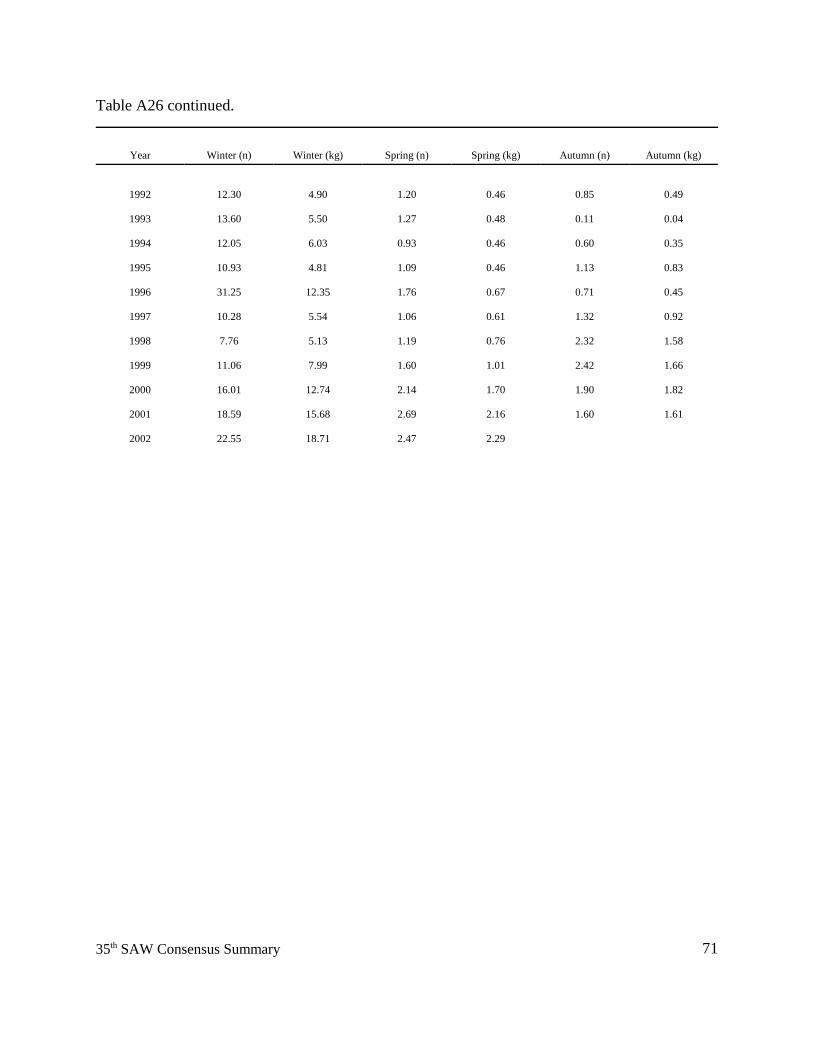
7135th SAW Consensus Summary
Table A26 continued.
Year Winter (n) Winter (kg) Spring (n) Spring (kg) Autumn (n) Autumn (kg)
1992 12.30 4.90 1.20 0.46 0.85 0.49
1993 13.60 5.50 1.27 0.48 0.11 0.04
1994 12.05 6.03 0.93 0.46 0.60 0.35
1995 10.93 4.81 1.09 0.46 1.13 0.83
1996 31.25 12.35 1.76 0.67 0.71 0.45
1997 10.28 5.54 1.06 0.61 1.32 0.92
1998 7.76 5.13 1.19 0.76 2.32 1.58
1999 11.06 7.99 1.60 1.01 2.42 1.66
2000 16.01 12.74 2.14 1.70 1.90 1.82
2001 18.59 15.68 2.69 2.16 1.60 1.61
2002 22.55 18.71 2.47 2.29
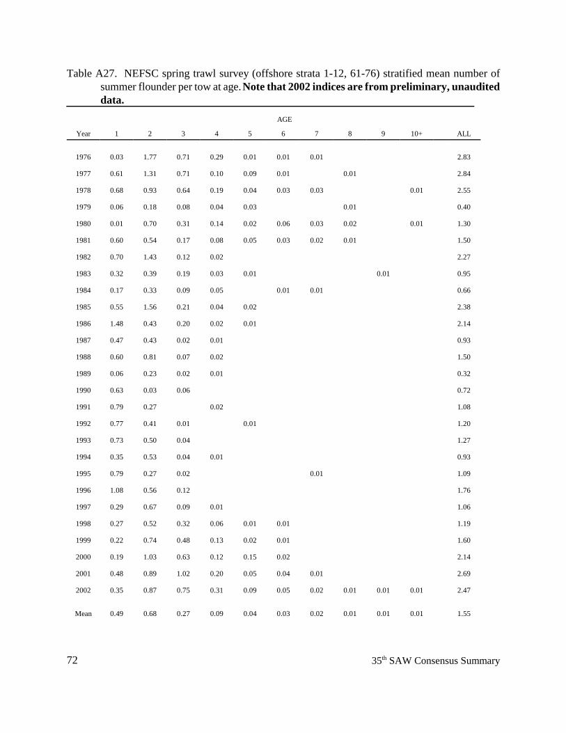
72 35th SAW Consensus Summary
Table A27. NEFSC spring trawl survey (offshore strata 1-12, 61-76) stratified mean number ofsummer flounder per tow at age. Note that 2002 indices are from preliminary, unauditeddata.
AGE
Year 1 2 3 4 5 6 7 8 9 10+ ALL
1976 0.03 1.77 0.71 0.29 0.01 0.01 0.01 2.83
1977 0.61 1.31 0.71 0.10 0.09 0.01 0.01 2.84
1978 0.68 0.93 0.64 0.19 0.04 0.03 0.03 0.01 2.55
1979 0.06 0.18 0.08 0.04 0.03 0.01 0.40
1980 0.01 0.70 0.31 0.14 0.02 0.06 0.03 0.02 0.01 1.30
1981 0.60 0.54 0.17 0.08 0.05 0.03 0.02 0.01 1.50
1982 0.70 1.43 0.12 0.02 2.27
1983 0.32 0.39 0.19 0.03 0.01 0.01 0.95
1984 0.17 0.33 0.09 0.05 0.01 0.01 0.66
1985 0.55 1.56 0.21 0.04 0.02 2.38
1986 1.48 0.43 0.20 0.02 0.01 2.14
1987 0.47 0.43 0.02 0.01 0.93
1988 0.60 0.81 0.07 0.02 1.50
1989 0.06 0.23 0.02 0.01 0.32
1990 0.63 0.03 0.06 0.72
1991 0.79 0.27 0.02 1.08
1992 0.77 0.41 0.01 0.01 1.20
1993 0.73 0.50 0.04 1.27
1994 0.35 0.53 0.04 0.01 0.93
1995 0.79 0.27 0.02 0.01 1.09
1996 1.08 0.56 0.12 1.76
1997 0.29 0.67 0.09 0.01 1.06
1998 0.27 0.52 0.32 0.06 0.01 0.01 1.19
1999 0.22 0.74 0.48 0.13 0.02 0.01 1.60
2000 0.19 1.03 0.63 0.12 0.15 0.02 2.14
2001 0.48 0.89 1.02 0.20 0.05 0.04 0.01 2.69
2002 0.35 0.87 0.75 0.31 0.09 0.05 0.02 0.01 0.01 0.01 2.47
Mean 0.49 0.68 0.27 0.09 0.04 0.03 0.02 0.01 0.01 0.01 1.55
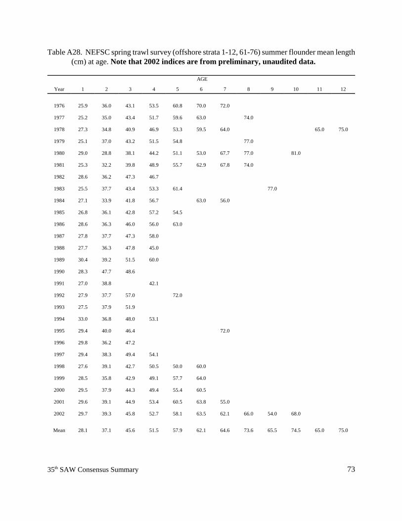
7335th SAW Consensus Summary
Table A28. NEFSC spring trawl survey (offshore strata 1-12, 61-76) summer flounder mean length(cm) at age. Note that 2002 indices are from preliminary, unaudited data.
AGE
Year 1 2 3 4 5 6 7 8 9 10 11 12
1976 25.9 36.0 43.1 53.5 60.8 70.0 72.0
1977 25.2 35.0 43.4 51.7 59.6 63.0 74.0
1978 27.3 34.8 40.9 46.9 53.3 59.5 64.0 65.0 75.0
1979 25.1 37.0 43.2 51.5 54.8 77.0
1980 29.0 28.8 38.1 44.2 51.1 53.0 67.7 77.0 81.0
1981 25.3 32.2 39.8 48.9 55.7 62.9 67.8 74.0
1982 28.6 36.2 47.3 46.7
1983 25.5 37.7 43.4 53.3 61.4 77.0
1984 27.1 33.9 41.8 56.7 63.0 56.0
1985 26.8 36.1 42.8 57.2 54.5
1986 28.6 36.3 46.0 56.0 63.0
1987 27.8 37.7 47.3 58.0
1988 27.7 36.3 47.8 45.0
1989 30.4 39.2 51.5 60.0
1990 28.3 47.7 48.6
1991 27.0 38.8 42.1
1992 27.9 37.7 57.0 72.0
1993 27.5 37.9 51.9
1994 33.0 36.8 48.0 53.1
1995 29.4 40.0 46.4 72.0
1996 29.8 36.2 47.2
1997 29.4 38.3 49.4 54.1
1998 27.6 39.1 42.7 50.5 50.0 60.0
1999 28.5 35.8 42.9 49.1 57.7 64.0
2000 29.5 37.9 44.3 49.4 55.4 60.5
2001 29.6 39.1 44.9 53.4 60.5 63.8 55.0
2002 29.7 39.3 45.8 52.7 58.1 63.5 62.1 66.0 54.0 68.0
Mean 28.1 37.1 45.6 51.5 57.9 62.1 64.6 73.6 65.5 74.5 65.0 75.0
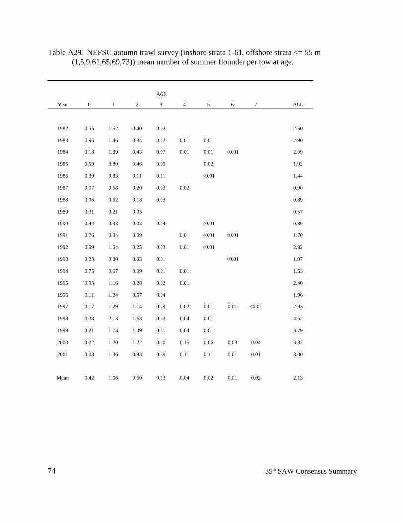
74 35th SAW Consensus Summary
Table A29. NEFSC autumn trawl survey (inshore strata 1-61, offshore strata <= 55 m(1,5,9,61,65,69,73)) mean number of summer flounder per tow at age.
AGE
Year 0 1 2 3 4 5 6 7 ALL
1982 0.55 1.52 0.40 0.03 2.50
1983 0.96 1.46 0.34 0.12 0.01 0.01 2.90
1984 0.18 1.39 0.43 0.07 0.01 0.01 <0.01 2.09
1985 0.59 0.80 0.46 0.05 0.02 1.92
1986 0.39 0.83 0.11 0.11 <0.01 1.44
1987 0.07 0.58 0.20 0.03 0.02 0.90
1988 0.06 0.62 0.18 0.03 0.89
1989 0.31 0.21 0.05 0.57
1990 0.44 0.38 0.03 0.04 <0.01 0.89
1991 0.76 0.84 0.09 0.01 <0.01 <0.01 1.70
1992 0.99 1.04 0.25 0.03 0.01 <0.01 2.32
1993 0.23 0.80 0.03 0.01 <0.01 1.07
1994 0.75 0.67 0.09 0.01 0.01 1.53
1995 0.93 1.16 0.28 0.02 0.01 2.40
1996 0.11 1.24 0.57 0.04 1.96
1997 0.17 1.29 1.14 0.29 0.02 0.01 0.01 <0.01 2.93
1998 0.38 2.13 1.63 0.33 0.04 0.01 4.52
1999 0.21 1.73 1.49 0.31 0.04 0.01 3.79
2000 0.22 1.20 1.22 0.40 0.15 0.06 0.03 0.04 3.32
2001 0.08 1.36 0.93 0.39 0.11 0.11 0.01 0.01 3.00
Mean 0.42 1.06 0.50 0.13 0.04 0.02 0.01 0.02 2.13
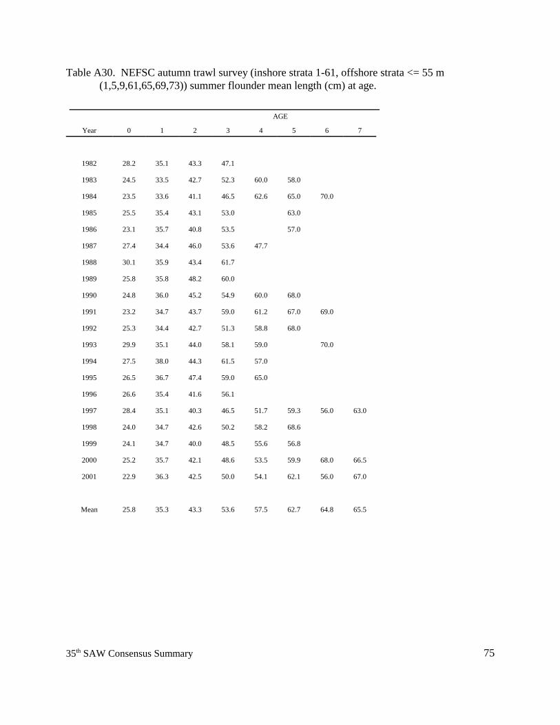
7535th SAW Consensus Summary
Table A30. NEFSC autumn trawl survey (inshore strata 1-61, offshore strata <= 55 m(1,5,9,61,65,69,73)) summer flounder mean length (cm) at age.
AGE
Year 0 1 2 3 4 5 6 7
1982 28.2 35.1 43.3 47.1
1983 24.5 33.5 42.7 52.3 60.0 58.0
1984 23.5 33.6 41.1 46.5 62.6 65.0 70.0
1985 25.5 35.4 43.1 53.0 63.0
1986 23.1 35.7 40.8 53.5 57.0
1987 27.4 34.4 46.0 53.6 47.7
1988 30.1 35.9 43.4 61.7
1989 25.8 35.8 48.2 60.0
1990 24.8 36.0 45.2 54.9 60.0 68.0
1991 23.2 34.7 43.7 59.0 61.2 67.0 69.0
1992 25.3 34.4 42.7 51.3 58.8 68.0
1993 29.9 35.1 44.0 58.1 59.0 70.0
1994 27.5 38.0 44.3 61.5 57.0
1995 26.5 36.7 47.4 59.0 65.0
1996 26.6 35.4 41.6 56.1
1997 28.4 35.1 40.3 46.5 51.7 59.3 56.0 63.0
1998 24.0 34.7 42.6 50.2 58.2 68.6
1999 24.1 34.7 40.0 48.5 55.6 56.8
2000 25.2 35.7 42.1 48.6 53.5 59.9 68.0 66.5
2001 22.9 36.3 42.5 50.0 54.1 62.1 56.0 67.0
Mean 25.8 35.3 43.3 53.6 57.5 62.7 64.8 65.5
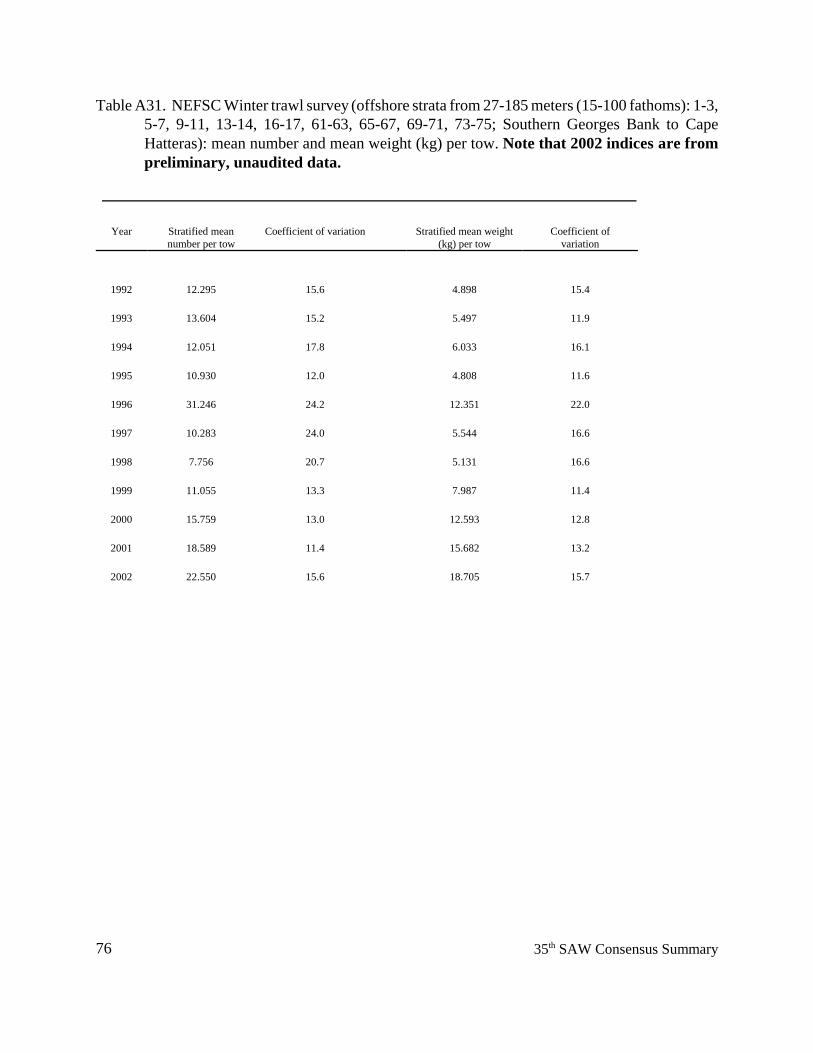
76 35th SAW Consensus Summary
Table A31. NEFSC Winter trawl survey (offshore strata from 27-185 meters (15-100 fathoms): 1-3,5-7, 9-11, 13-14, 16-17, 61-63, 65-67, 69-71, 73-75; Southern Georges Bank to CapeHatteras): mean number and mean weight (kg) per tow. Note that 2002 indices are frompreliminary, unaudited data.
Year Stratified meannumber per tow
Coefficient of variation Stratified mean weight(kg) per tow
Coefficient ofvariation
1992 12.295 15.6 4.898 15.4
1993 13.604 15.2 5.497 11.9
1994 12.051 17.8 6.033 16.1
1995 10.930 12.0 4.808 11.6
1996 31.246 24.2 12.351 22.0
1997 10.283 24.0 5.544 16.6
1998 7.756 20.7 5.131 16.6
1999 11.055 13.3 7.987 11.4
2000 15.759 13.0 12.593 12.8
2001 18.589 11.4 15.682 13.2
2002 22.550 15.6 18.705 15.7
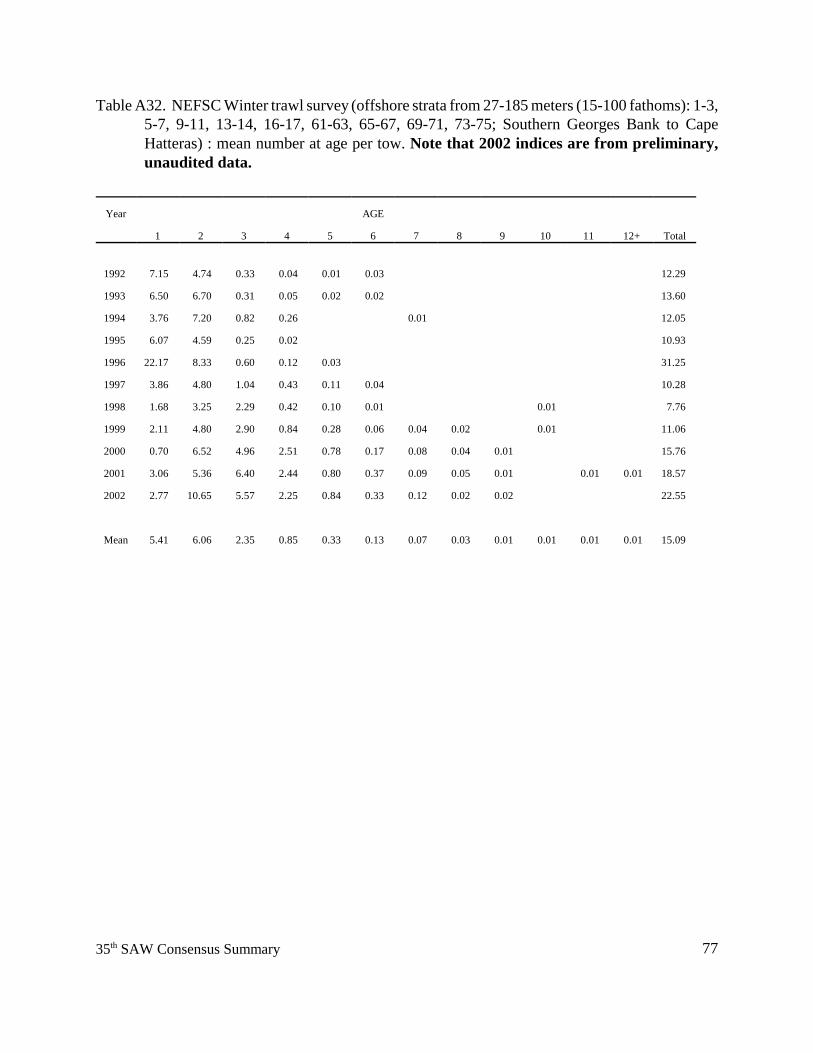
7735th SAW Consensus Summary
Table A32. NEFSC Winter trawl survey (offshore strata from 27-185 meters (15-100 fathoms): 1-3,5-7, 9-11, 13-14, 16-17, 61-63, 65-67, 69-71, 73-75; Southern Georges Bank to CapeHatteras) : mean number at age per tow. Note that 2002 indices are from preliminary,unaudited data.
Year AGE
1 2 3 4 5 6 7 8 9 10 11 12+ Total
1992 7.15 4.74 0.33 0.04 0.01 0.03 12.29
1993 6.50 6.70 0.31 0.05 0.02 0.02 13.60
1994 3.76 7.20 0.82 0.26 0.01 12.05
1995 6.07 4.59 0.25 0.02 10.93
1996 22.17 8.33 0.60 0.12 0.03 31.25
1997 3.86 4.80 1.04 0.43 0.11 0.04 10.28
1998 1.68 3.25 2.29 0.42 0.10 0.01 0.01 7.76
1999 2.11 4.80 2.90 0.84 0.28 0.06 0.04 0.02 0.01 11.06
2000 0.70 6.52 4.96 2.51 0.78 0.17 0.08 0.04 0.01 15.76
2001 3.06 5.36 6.40 2.44 0.80 0.37 0.09 0.05 0.01 0.01 0.01 18.57
2002 2.77 10.65 5.57 2.25 0.84 0.33 0.12 0.02 0.02 22.55
Mean 5.41 6.06 2.35 0.85 0.33 0.13 0.07 0.03 0.01 0.01 0.01 0.01 15.09
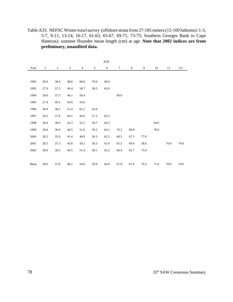
78 35th SAW Consensus Summary
Table A33. NEFSC Winter trawl survey (offshore strata from 27-185 meters (15-100 fathoms): 1-3,5-7, 9-11, 13-14, 16-17, 61-63, 65-67, 69-71, 73-75; Southern Georges Bank to CapeHatteras): summer flounder mean length (cm) at age. Note that 2002 indices are frompreliminary, unaudited data.
AGE
Year 1 2 3 4 5 6 7 8 9 10 11 12+
1992 28.0 38.4 48.8 60.0 70.0 69.0
1993 27.9 37.3 49.4 58.7 58.5 65.0
1994 28.0 37.5 46.1 56.4 69.0
1995 27.4 40.2 50.8 59.6
1996 30.9 38.2 51.4 61.2 63.6
1997 29.2 37.8 44.5 50.0 57.3 62.5
1998 28.4 38.0 43.3 52.2 59.7 66.3 64.0
1999 28.4 36.9 44.5 51.6 59.2 64.1 70.2 68.8 78.0
2000 28.2 35.9 41.4 49.0 56.3 62.2 68.2 67.1 77.0
2001 28.3 37.3 43.6 50.2 56.3 61.0 65.3 69.4 58.6 70.0 74.0
2002 30.0 38.5 44.5 51.4 58.1 62.2 66.4 62.7 75.0
Mean 28.6 37.8 46.2 54.6 59.9 64.0 67.8 67.0 70.2 71.0 70.0 74.0
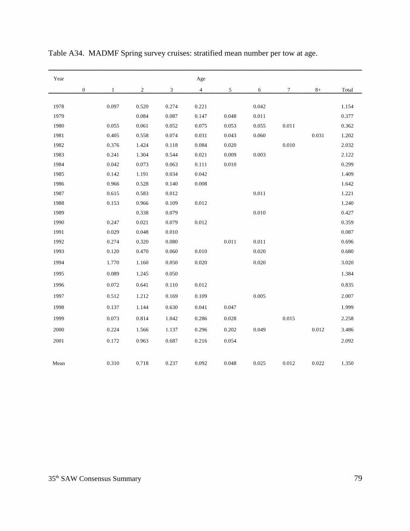
7935th SAW Consensus Summary
Table A34. MADMF Spring survey cruises: stratified mean number per tow at age.
Year Age
0 1 2 3 4 5 6 7 8+ Total
1978 0.097 0.520 0.274 0.221 0.042 1.154
1979 0.084 0.087 0.147 0.048 0.011 0.377
1980 0.055 0.061 0.052 0.075 0.053 0.055 0.011 0.362
1981 0.405 0.558 0.074 0.031 0.043 0.060 0.031 1.202
1982 0.376 1.424 0.118 0.084 0.020 0.010 2.032
1983 0.241 1.304 0.544 0.021 0.009 0.003 2.122
1984 0.042 0.073 0.063 0.111 0.010 0.299
1985 0.142 1.191 0.034 0.042 1.409
1986 0.966 0.528 0.140 0.008 1.642
1987 0.615 0.583 0.012 0.011 1.221
1988 0.153 0.966 0.109 0.012 1.240
1989 0.338 0.079 0.010 0.427
1990 0.247 0.021 0.079 0.012 0.359
1991 0.029 0.048 0.010 0.087
1992 0.274 0.320 0.080 0.011 0.011 0.696
1993 0.120 0.470 0.060 0.010 0.020 0.680
1994 1.770 1.160 0.050 0.020 0.020 3.020
1995 0.089 1.245 0.050 1.384
1996 0.072 0.641 0.110 0.012 0.835
1997 0.512 1.212 0.169 0.109 0.005 2.007
1998 0.137 1.144 0.630 0.041 0.047 1.999
1999 0.073 0.814 1.042 0.286 0.028 0.015 2.258
2000 0.224 1.566 1.137 0.296 0.202 0.049 0.012 3.486
2001 0.172 0.963 0.687 0.216 0.054 2.092
Mean 0.310 0.718 0.237 0.092 0.048 0.025 0.012 0.022 1.350
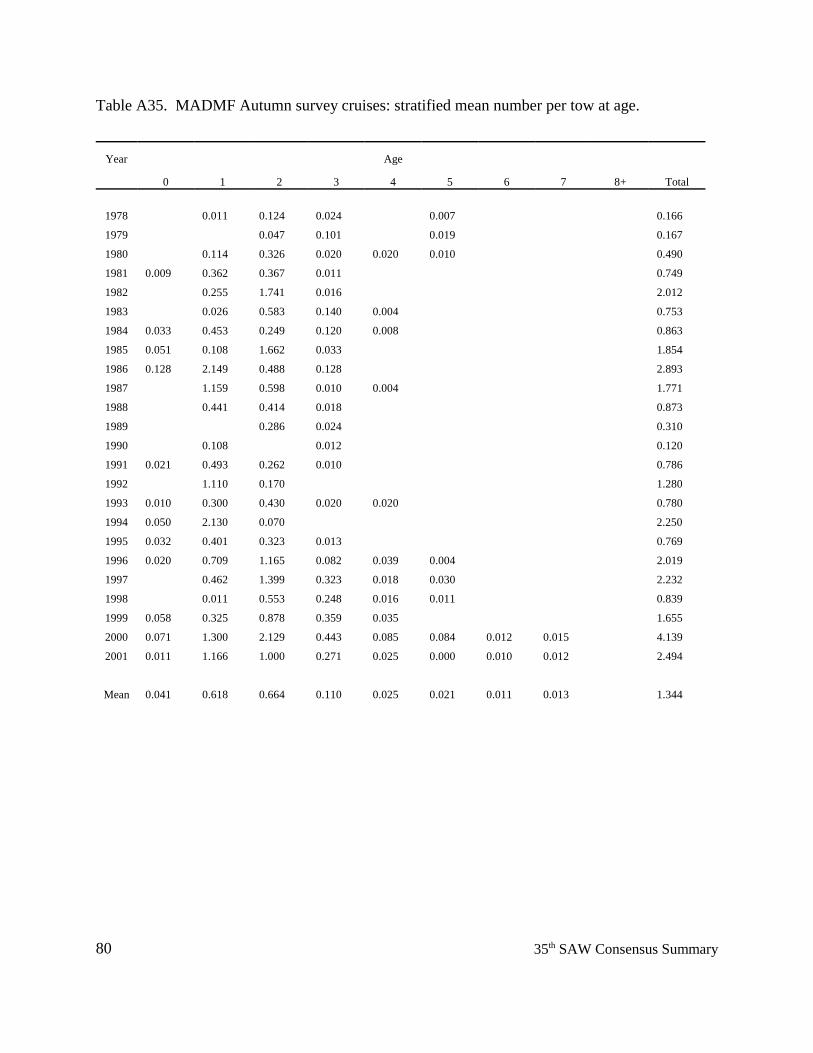
80 35th SAW Consensus Summary
Table A35. MADMF Autumn survey cruises: stratified mean number per tow at age.
Year Age
0 1 2 3 4 5 6 7 8+ Total
1978 0.011 0.124 0.024 0.007 0.166
1979 0.047 0.101 0.019 0.167
1980 0.114 0.326 0.020 0.020 0.010 0.490
1981 0.009 0.362 0.367 0.011 0.749
1982 0.255 1.741 0.016 2.012
1983 0.026 0.583 0.140 0.004 0.753
1984 0.033 0.453 0.249 0.120 0.008 0.863
1985 0.051 0.108 1.662 0.033 1.854
1986 0.128 2.149 0.488 0.128 2.893
1987 1.159 0.598 0.010 0.004 1.771
1988 0.441 0.414 0.018 0.873
1989 0.286 0.024 0.310
1990 0.108 0.012 0.120
1991 0.021 0.493 0.262 0.010 0.786
1992 1.110 0.170 1.280
1993 0.010 0.300 0.430 0.020 0.020 0.780
1994 0.050 2.130 0.070 2.250
1995 0.032 0.401 0.323 0.013 0.769
1996 0.020 0.709 1.165 0.082 0.039 0.004 2.019
1997 0.462 1.399 0.323 0.018 0.030 2.232
1998 0.011 0.553 0.248 0.016 0.011 0.839
1999 0.058 0.325 0.878 0.359 0.035 1.655
2000 0.071 1.300 2.129 0.443 0.085 0.084 0.012 0.015 4.139
2001 0.011 1.166 1.000 0.271 0.025 0.000 0.010 0.012 2.494
Mean 0.041 0.618 0.664 0.110 0.025 0.021 0.011 0.013 1.344
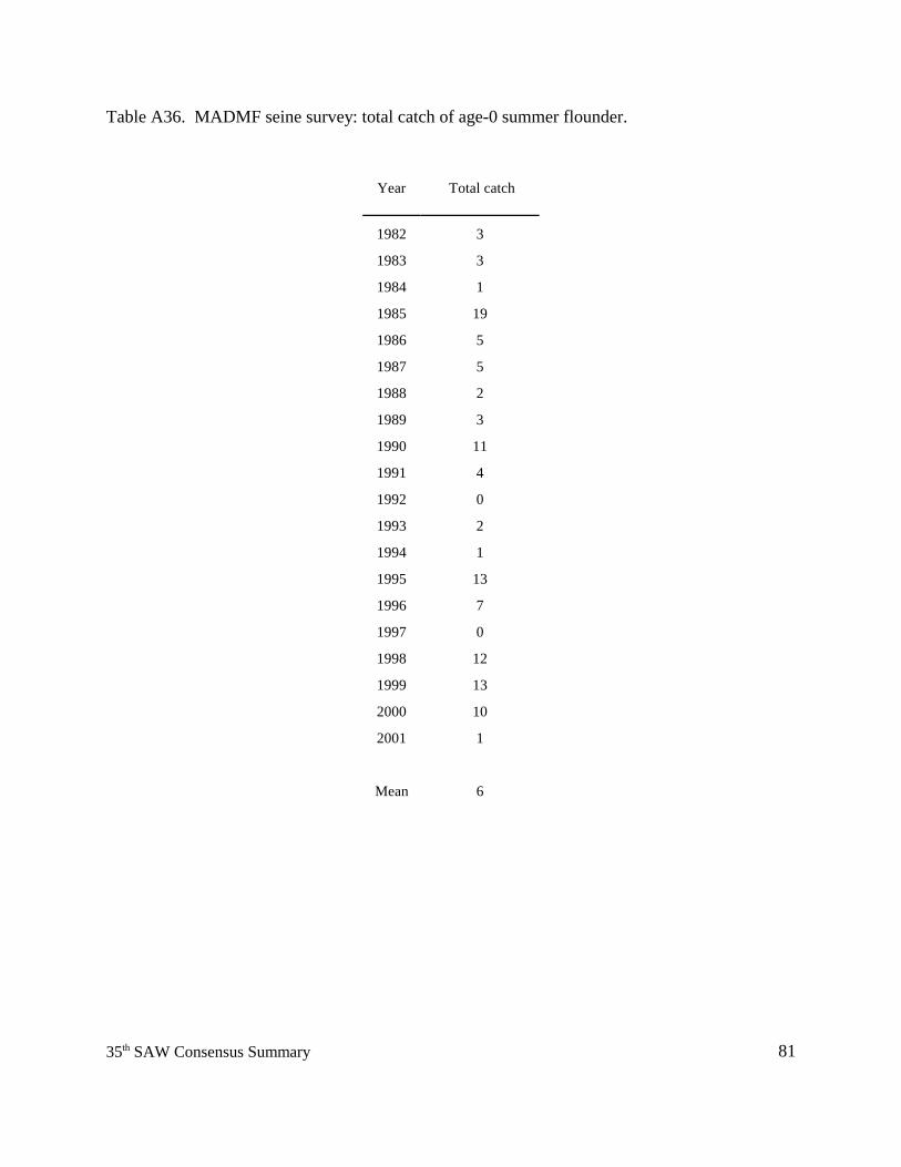
8135th SAW Consensus Summary
Table A36. MADMF seine survey: total catch of age-0 summer flounder.
Year Total catch
1982 3
1983 3
1984 1
1985 19
1986 5
1987 5
1988 2
1989 3
1990 11
1991 4
1992 0
1993 2
1994 1
1995 13
1996 7
1997 0
1998 12
1999 13
2000 10
2001 1
Mean 6
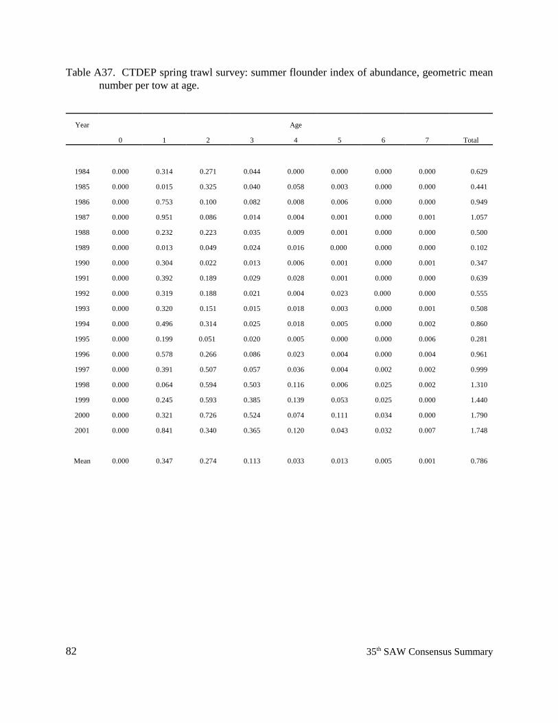
82 35th SAW Consensus Summary
Table A37. CTDEP spring trawl survey: summer flounder index of abundance, geometric meannumber per tow at age.
Year Age
0 1 2 3 4 5 6 7 Total
1984 0.000 0.314 0.271 0.044 0.000 0.000 0.000 0.000 0.629
1985 0.000 0.015 0.325 0.040 0.058 0.003 0.000 0.000 0.441
1986 0.000 0.753 0.100 0.082 0.008 0.006 0.000 0.000 0.949
1987 0.000 0.951 0.086 0.014 0.004 0.001 0.000 0.001 1.057
1988 0.000 0.232 0.223 0.035 0.009 0.001 0.000 0.000 0.500
1989 0.000 0.013 0.049 0.024 0.016 0.000 0.000 0.000 0.102
1990 0.000 0.304 0.022 0.013 0.006 0.001 0.000 0.001 0.347
1991 0.000 0.392 0.189 0.029 0.028 0.001 0.000 0.000 0.639
1992 0.000 0.319 0.188 0.021 0.004 0.023 0.000 0.000 0.555
1993 0.000 0.320 0.151 0.015 0.018 0.003 0.000 0.001 0.508
1994 0.000 0.496 0.314 0.025 0.018 0.005 0.000 0.002 0.860
1995 0.000 0.199 0.051 0.020 0.005 0.000 0.000 0.006 0.281
1996 0.000 0.578 0.266 0.086 0.023 0.004 0.000 0.004 0.961
1997 0.000 0.391 0.507 0.057 0.036 0.004 0.002 0.002 0.999
1998 0.000 0.064 0.594 0.503 0.116 0.006 0.025 0.002 1.310
1999 0.000 0.245 0.593 0.385 0.139 0.053 0.025 0.000 1.440
2000 0.000 0.321 0.726 0.524 0.074 0.111 0.034 0.000 1.790
2001 0.000 0.841 0.340 0.365 0.120 0.043 0.032 0.007 1.748
Mean 0.000 0.347 0.274 0.113 0.033 0.013 0.005 0.001 0.786
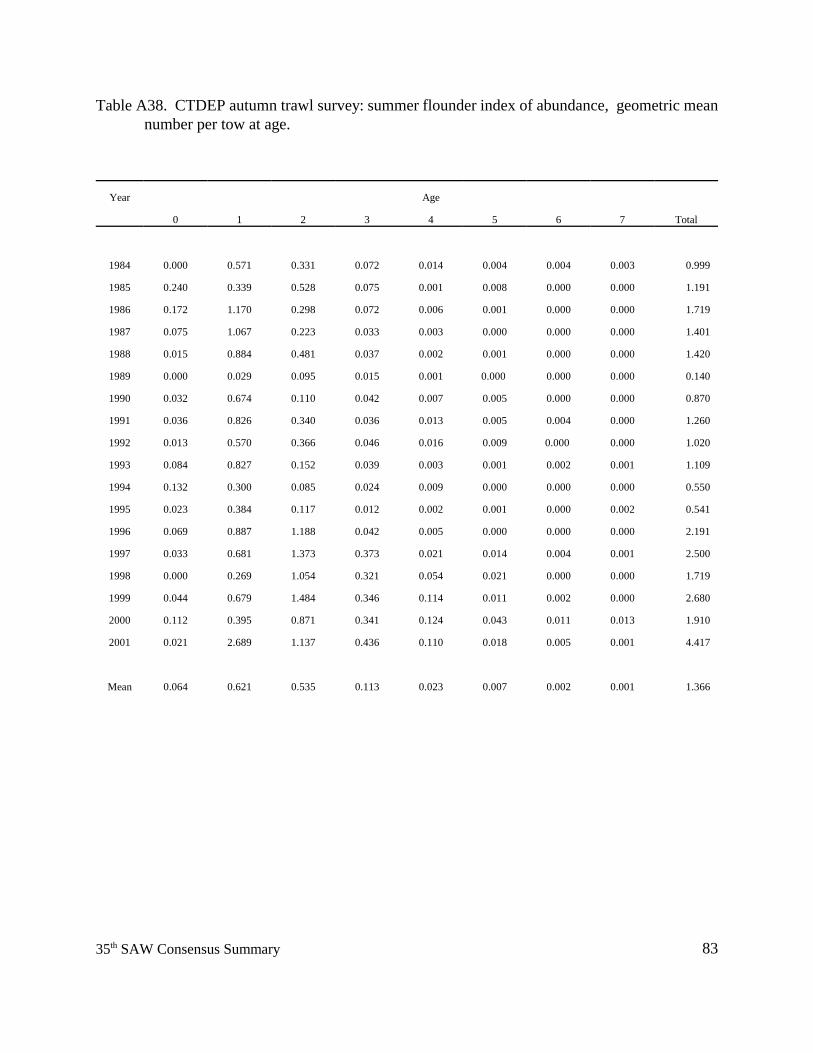
8335th SAW Consensus Summary
Table A38. CTDEP autumn trawl survey: summer flounder index of abundance, geometric meannumber per tow at age.
Year Age
0 1 2 3 4 5 6 7 Total
1984 0.000 0.571 0.331 0.072 0.014 0.004 0.004 0.003 0.999
1985 0.240 0.339 0.528 0.075 0.001 0.008 0.000 0.000 1.191
1986 0.172 1.170 0.298 0.072 0.006 0.001 0.000 0.000 1.719
1987 0.075 1.067 0.223 0.033 0.003 0.000 0.000 0.000 1.401
1988 0.015 0.884 0.481 0.037 0.002 0.001 0.000 0.000 1.420
1989 0.000 0.029 0.095 0.015 0.001 0.000 0.000 0.000 0.140
1990 0.032 0.674 0.110 0.042 0.007 0.005 0.000 0.000 0.870
1991 0.036 0.826 0.340 0.036 0.013 0.005 0.004 0.000 1.260
1992 0.013 0.570 0.366 0.046 0.016 0.009 0.000 0.000 1.020
1993 0.084 0.827 0.152 0.039 0.003 0.001 0.002 0.001 1.109
1994 0.132 0.300 0.085 0.024 0.009 0.000 0.000 0.000 0.550
1995 0.023 0.384 0.117 0.012 0.002 0.001 0.000 0.002 0.541
1996 0.069 0.887 1.188 0.042 0.005 0.000 0.000 0.000 2.191
1997 0.033 0.681 1.373 0.373 0.021 0.014 0.004 0.001 2.500
1998 0.000 0.269 1.054 0.321 0.054 0.021 0.000 0.000 1.719
1999 0.044 0.679 1.484 0.346 0.114 0.011 0.002 0.000 2.680
2000 0.112 0.395 0.871 0.341 0.124 0.043 0.011 0.013 1.910
2001 0.021 2.689 1.137 0.436 0.110 0.018 0.005 0.001 4.417
Mean 0.064 0.621 0.535 0.113 0.023 0.007 0.002 0.001 1.366
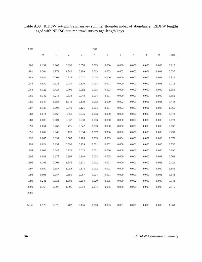
84 35th SAW Consensus Summary
Table A39. RIDFW autumn trawl survey summer flounder index of abundance. RIDFW lengthsaged with NEFSC autumn trawl survey age-length keys.
Year Age
0 1 2 3 4 5 6 7 8 9 Total
1980 0.131 0.203 0.392 0.074 0.013 0.000 0.000 0.000 0.000 0.000 0.813
1981 0.304 0.971 1.740 0.199 0.013 0.003 0.002 0.002 0.001 0.001 3.236
1982 0.024 0.209 0.516 0.071 0.005 0.000 0.000 0.000 0.000 0.001 0.826
1983 0.030 0.135 0.420 0.110 0.014 0.001 0.000 0.001 0.000 0.001 0.712
1984 0.122 0.424 0.701 0.092 0.013 0.003 0.000 0.000 0.000 0.000 1.355
1985 0.342 0.218 0.338 0.048 0.004 0.001 0.000 0.001 0.000 0.000 0.952
1986 0.547 1.183 1.518 0.179 0.012 0.000 0.002 0.001 0.001 0.001 3.444
1987 0.135 0.503 0.579 0.121 0.014 0.001 0.003 0.003 0.001 0.000 1.360
1988 0.014 0.167 0.351 0.036 0.003 0.000 0.000 0.000 0.000 0.000 0.571
1989 0.000 0.001 0.037 0.030 0.003 0.000 0.000 0.000 0.000 0.000 0.071
1990 0.051 0.262 0.475 0.042 0.003 0.000 0.000 0.000 0.000 0.000 0.833
1991 0.002 0.060 0.128 0.034 0.007 0.000 0.000 0.000 0.000 0.000 0.231
1992 0.065 0.394 0.685 0.185 0.033 0.003 0.004 0.001 0.001 0.000 1.371
1993 0.024 0.152 0.396 0.139 0.021 0.002 0.000 0.001 0.000 0.000 0.735
1994 0.005 0.045 0.126 0.013 0.001 0.000 0.000 0.000 0.000 0.000 0.190
1995 0.031 0.175 0.393 0.140 0.013 0.005 0.000 0.004 0.000 0.001 0.762
1996 0.193 0.704 1.346 0.171 0.012 0.001 0.000 0.001 0.000 0.001 2.429
1997 0.080 0.557 1.053 0.174 0.012 0.003 0.000 0.002 0.000 0.000 1.881
1998 0.008 0.087 0.359 0.087 0.004 0.001 0.000 0.001 0.000 0.001 0.548
1999 0.241 0.931 1.888 0.254 0.020 0.005 0.000 0.002 0.000 0.000 3.341
2000 0.365 0.506 1.305 0.654 0.054 0.035 0.000 0.000 0.000 0.000 2.919
2001
Mean 0.129 0.376 0.702 0.136 0.013 0.003 0.001 0.001 0.000 0.000 1.361
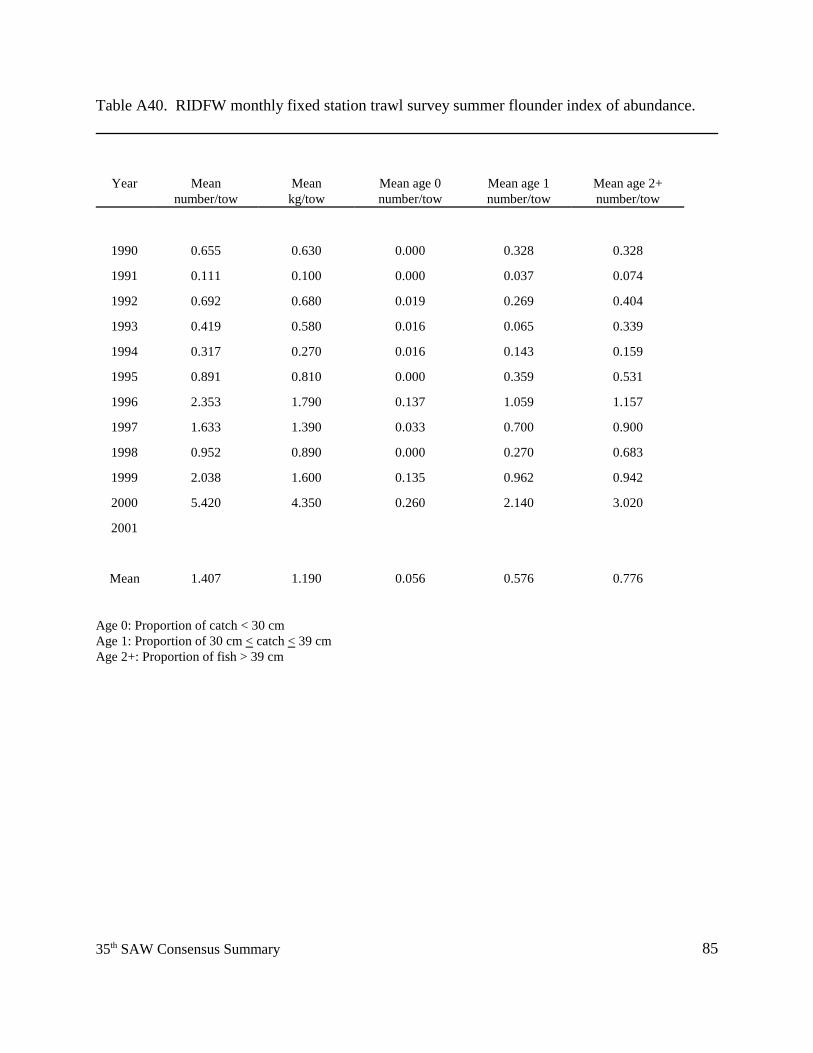
8535th SAW Consensus Summary
Table A40. RIDFW monthly fixed station trawl survey summer flounder index of abundance.
Year Meannumber/tow
Meankg/tow
Mean age 0number/tow
Mean age 1number/tow
Mean age 2+number/tow
1990 0.655 0.630 0.000 0.328 0.328
1991 0.111 0.100 0.000 0.037 0.074
1992 0.692 0.680 0.019 0.269 0.404
1993 0.419 0.580 0.016 0.065 0.339
1994 0.317 0.270 0.016 0.143 0.159
1995 0.891 0.810 0.000 0.359 0.531
1996 2.353 1.790 0.137 1.059 1.157
1997 1.633 1.390 0.033 0.700 0.900
1998 0.952 0.890 0.000 0.270 0.683
1999 2.038 1.600 0.135 0.962 0.942
2000 5.420 4.350 0.260 2.140 3.020
2001
Mean 1.407 1.190 0.056 0.576 0.776
Age 0: Proportion of catch < 30 cmAge 1: Proportion of 30 cm < catch < 39 cmAge 2+: Proportion of fish > 39 cm
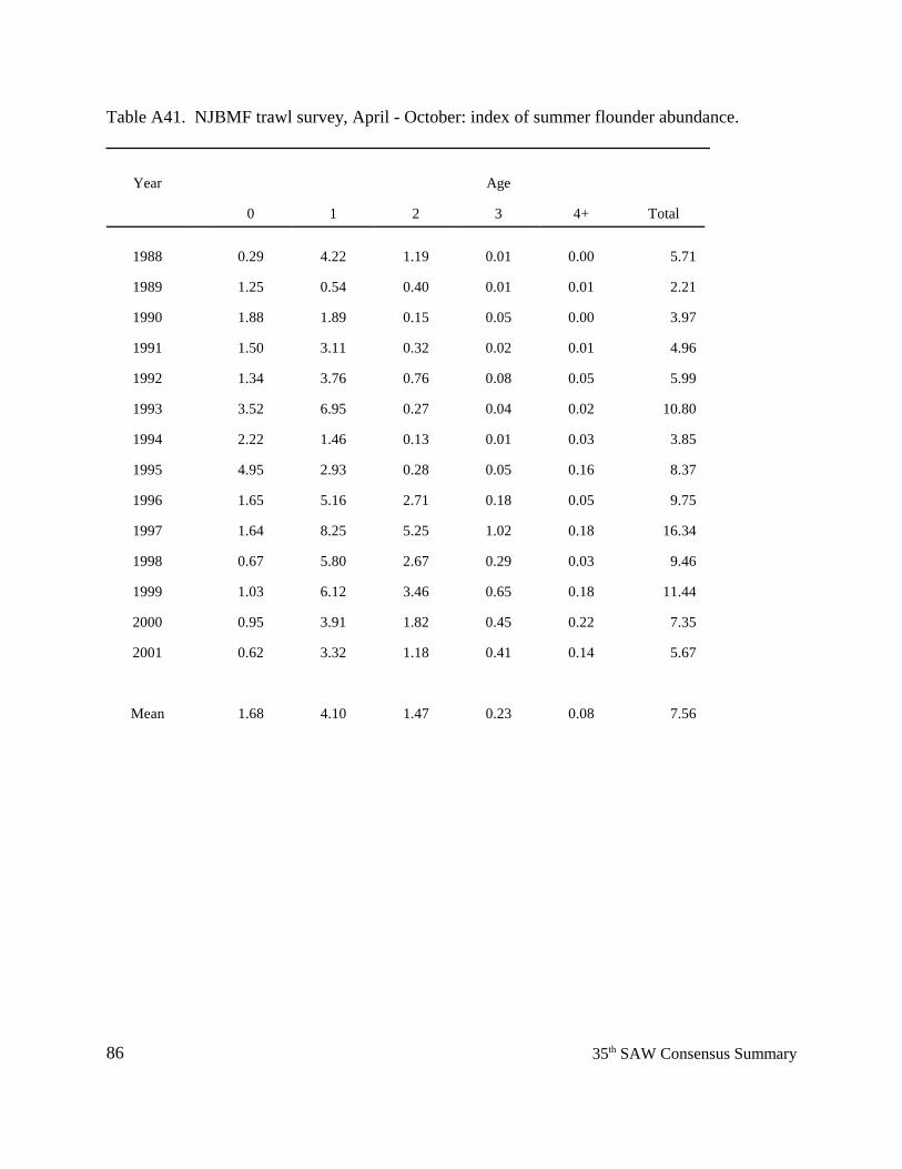
86 35th SAW Consensus Summary
Table A41. NJBMF trawl survey, April - October: index of summer flounder abundance.
Year Age
0 1 2 3 4+ Total
1988 0.29 4.22 1.19 0.01 0.00 5.71
1989 1.25 0.54 0.40 0.01 0.01 2.21
1990 1.88 1.89 0.15 0.05 0.00 3.97
1991 1.50 3.11 0.32 0.02 0.01 4.96
1992 1.34 3.76 0.76 0.08 0.05 5.99
1993 3.52 6.95 0.27 0.04 0.02 10.80
1994 2.22 1.46 0.13 0.01 0.03 3.85
1995 4.95 2.93 0.28 0.05 0.16 8.37
1996 1.65 5.16 2.71 0.18 0.05 9.75
1997 1.64 8.25 5.25 1.02 0.18 16.34
1998 0.67 5.80 2.67 0.29 0.03 9.46
1999 1.03 6.12 3.46 0.65 0.18 11.44
2000 0.95 3.91 1.82 0.45 0.22 7.35
2001 0.62 3.32 1.18 0.41 0.14 5.67
Mean 1.68 4.10 1.47 0.23 0.08 7.56
8735th SAW Consensus Summary
Table A42. DEDFW 16 foot trawl survey: index of summer flounder recruitment at age-0 in theDelaware Estuary.
Year Geometric Meannumberper tow
1980 0.12
1981 0.06
1982 0.11
1983 0.03
1984 0.08
1985 0.06
1986 0.10
1987 0.14
1988 0.01
1989 0.12
1990 0.23
1991 0.07
1992 0.31
1993 0.02
1994 0.29
1995 0.17
1996 0.03
1997 0.02
1998 0.03
1999 0.05
2000 0.18
2001 0.07
Mean 0.10
88 35th SAW Consensus Summary
Table A43. DEDFW 16 foot trawl survey: index of summer flounder recruitment at age-0 in theDelaware Inland Bays.
Year Geometric Meannumberper tow
1986 0.01
1987 0.00
1988 0.00
1989 0.15
1990 0.02
1991 0.94
1992 0.06
1993 0.04
1994 0.70
1995 0.23
1996 0.05
1997 0.33
1998 0.99
1999 0.62
2000 0.70
2001 0.05
Mean 0.31
8935th SAW Consensus Summary
Table A44. DEDFW Delaware Bay 30 foot trawl survey: index of summer flounder abundance.
Year Age
0 1 2 3 4+ Total
1991 1.44 1.13 0.18 0.04 0.00 2.79
1992 0.47 0.28 0.08 0.00 0.00 0.83
1993 0.04 1.56 0.73 0.07 0.00 2.40
1994 2.28 0.14 0.22 0.08 0.00 2.72
1995 0.94 1.00 0.28 0.10 0.09 2.41
1996 0.46 0.73 0.48 0.10 0.02 1.79
1997 0.03 0.12 0.49 0.47 0.16 1.27
1998 0.11 0.31 0.83 0.29 0.12 1.66
1999 0.20 0.06 0.77 0.47 0.19 1.69
2000 0.79 0.24 0.30 0.28 0.23 1.84
2001 0.34 1.55 0.49 0.26 0.13 2.77
Mean 0.65 0.65 0.44 0.20 0.09 2.02
90 35th SAW Consensus Summary
Table A45. MD DNR Coastal Bays trawl survey: index of summer flounder recruitment at age-0.
Year Geometric mean Lower 95% CI Upper 95% CI
1972 12.3 6.5 21.8
1973 4.2 3.0 5.7
1974 5.1 3.9 6.6
1975 2.1 1.6 2.6
1976 1.9 1.4 2.6
1977 2.4 1.8 3.2
1978 3.2 2.4 4.1
1979 2.9 2.0 4.1
1980 4.2 2.6 6.2
1981 3.9 2.6 5.4
1982 2.0 0.8 3.7
1983 10.6 6.0 17.9
1984 5.4 3.1 8.7
1985 5.6 3.6 8.1
1986 16.2 10.1 25.2
1987 4.6 2.4 7.8
1988 0.5 0.3 0.8
1989 1.3 0.9 1.9
1990 2.1 1.6 2.7
1991 3.1 2.4 3.9
1992 3.5 2.5 4.7
1993 1.6 1.2 2.1
1994 8.2 6.5 10.3
1995 5.0 4.0 6.2
1996 2.6 2.0 3.2
1997 3.3 2.5 4.3
1998 5.2 4.2 6.6
1999 3.4 2.6 4.2
2000 4.1 3.1 5.2
2001 5.3 4.1 6.9
Mean 4.5
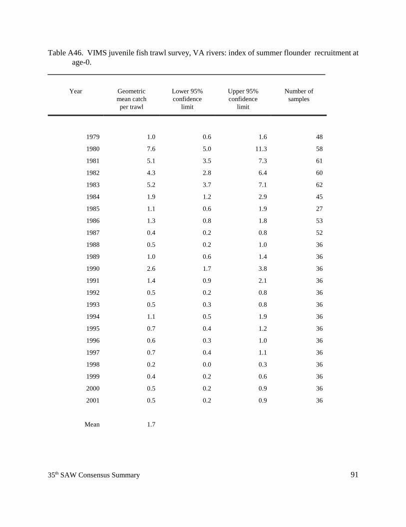
9135th SAW Consensus Summary
Table A46. VIMS juvenile fish trawl survey, VA rivers: index of summer flounder recruitment atage-0.
Year Geometricmean catchper trawl
Lower 95%confidence
limit
Upper 95%confidence
limit
Number ofsamples
1979 1.0 0.6 1.6 48
1980 7.6 5.0 11.3 58
1981 5.1 3.5 7.3 61
1982 4.3 2.8 6.4 60
1983 5.2 3.7 7.1 62
1984 1.9 1.2 2.9 45
1985 1.1 0.6 1.9 27
1986 1.3 0.8 1.8 53
1987 0.4 0.2 0.8 52
1988 0.5 0.2 1.0 36
1989 1.0 0.6 1.4 36
1990 2.6 1.7 3.8 36
1991 1.4 0.9 2.1 36
1992 0.5 0.2 0.8 36
1993 0.5 0.3 0.8 36
1994 1.1 0.5 1.9 36
1995 0.7 0.4 1.2 36
1996 0.6 0.3 1.0 36
1997 0.7 0.4 1.1 36
1998 0.2 0.0 0.3 36
1999 0.4 0.2 0.6 36
2000 0.5 0.2 0.9 36
2001 0.5 0.2 0.9 36
Mean 1.7
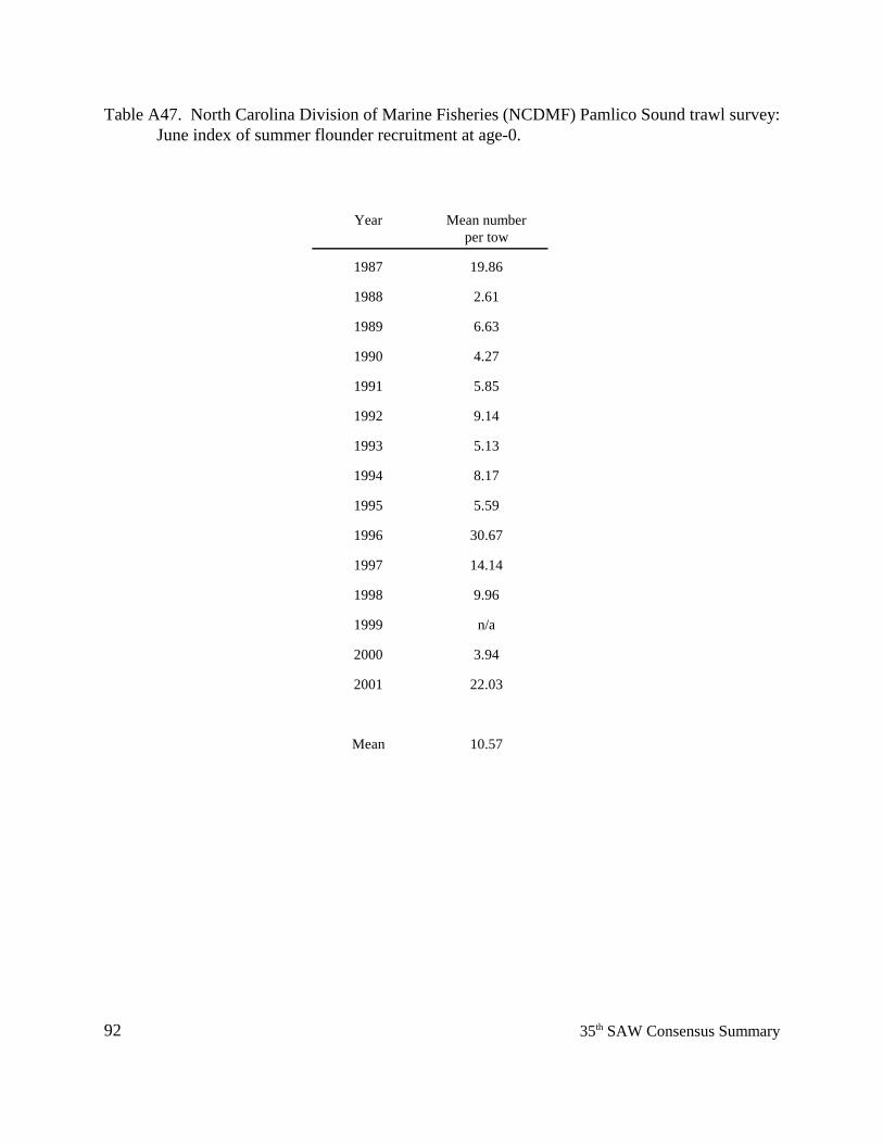
92 35th SAW Consensus Summary
Table A47. North Carolina Division of Marine Fisheries (NCDMF) Pamlico Sound trawl survey:June index of summer flounder recruitment at age-0.
Year Mean numberper tow
1987 19.86
1988 2.61
1989 6.63
1990 4.27
1991 5.85
1992 9.14
1993 5.13
1994 8.17
1995 5.59
1996 30.67
1997 14.14
1998 9.96
1999 n/a
2000 3.94
2001 22.03
Mean 10.57
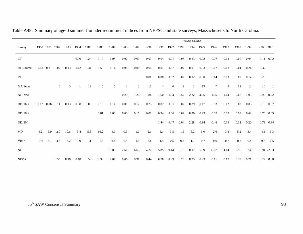
9335th SAW Consensus Summary
Table A48. Summary of age-0 summer flounder recruitment indices from NEFSC and state surveys, Massachusetts to North Carolina.
YEAR CLASS
Survey 1980 1981 1982 1983 1984 1985 1986 1987 1988 1989 1990 1991 1992 1993 1994 1995 1996 1997 1998 1999 2000 2001
CT 0.00 0.24 0.17 0.08 0.02 0.00 0.03 0.04 0.01 0.08 0.13 0.02 0.07 0.03 0.00 0.04 0.11 0.02
RI Autumn 0.13 0.31 0.02 0.03 0.12 0.34 0.55 0.14 0.01 0.00 0.05 0.01 0.07 0.02 0.01 0.03 0.17 0.08 0.01 0.24 0.37
RI 0.00 0.00 0.02 0.02 0.02 0.00 0.14 0.03 0.00 0.14 0.26
MA Seine 3 3 1 19 5 5 2 3 11 4 0 2 1 13 7 0 12 13 10 1
NJ Trawl 0.29 1.25 1.88 1.50 1.34 3.52 2.22 4.95 1.65 1.64 0.67 1.03 0.95 0.62
DE: 16 ft 0.12 0.06 0.11 0.03 0.08 0.06 0.10 0.14 0.01 0.12 0.23 0.07 0.31 0.02 0.29 0.17 0.03 0.02 0.03 0.05 0.18 0.07
DE: 16 ft 0.01 0.00 0.00 0.15 0.02 0.94 0.06 0.04 0.70 0.23 0.05 0.33 0.99 0.62 0.70 0.05
DE: 30ft 1.44 0.47 0.04 2.28 0.94 0.46 0.03 0.11 0.20 0.79 0.34
MD 4.2 3.9 2.0 10.6 5.4 5.6 16.2 4.6 0.5 1.3 2.1 3.1 3.5 1.6 8.2 5.0 2.6 3.3 5.2 3.4 4.1 5.3
VIMS 7.6 5.1 4.3 5.2 1.9 1.1 1.3 0.4 0.5 1.0 2.6 1.4 0.5 0.5 1.1 0.7 0.6 0.7 0.2 0.4 0.5 0.5
NC 19.86 2.61 6.63 4.27 5.85 9.14 5.13 8.17 5.59 30.67 14.14 9.96 n/a 3.94 22.03
NEFSC 0.55 0.96 0.18 0.59 0.39 0.07 0.06 0.31 0.44 0.76 0.99 0.23 0.75 0.93 0.11 0.17 0.38 0.21 0.22 0.08
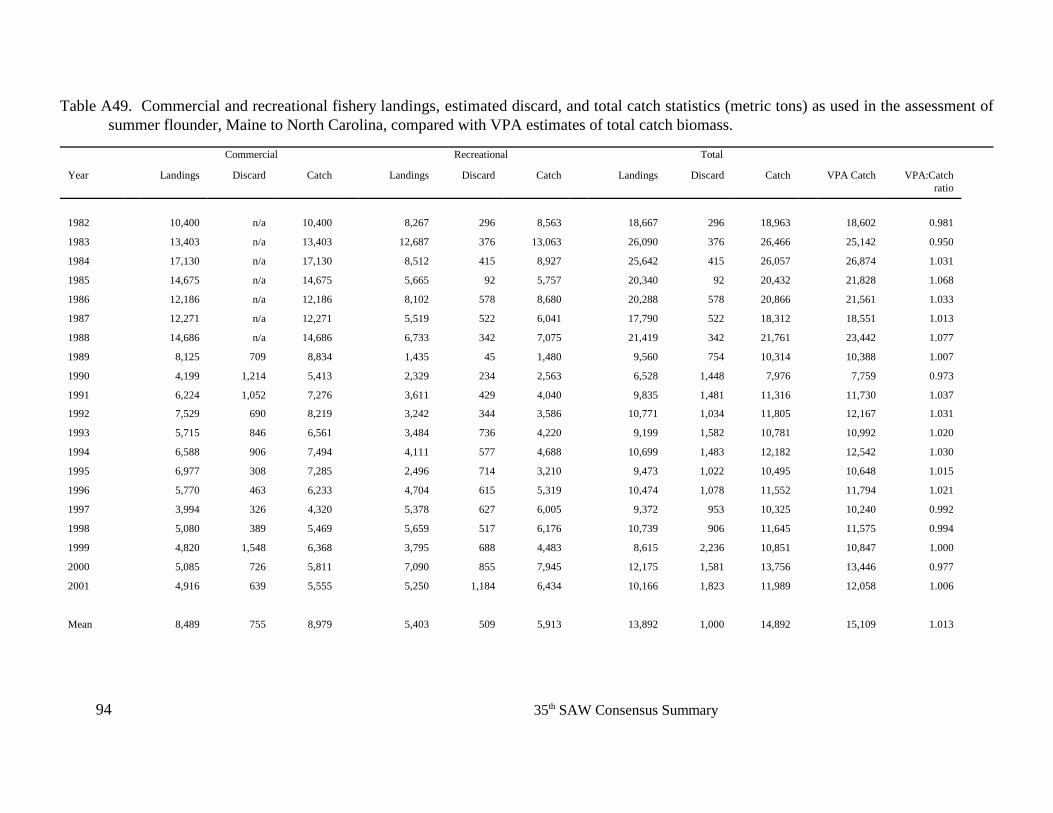
94 35th SAW Consensus Summary
Table A49. Commercial and recreational fishery landings, estimated discard, and total catch statistics (metric tons) as used in the assessment ofsummer flounder, Maine to North Carolina, compared with VPA estimates of total catch biomass.
Commercial Recreational Total
Year Landings Discard Catch Landings Discard Catch Landings Discard Catch VPA Catch VPA:Catchratio
1982 10,400 n/a 10,400 8,267 296 8,563 18,667 296 18,963 18,602 0.981
1983 13,403 n/a 13,403 12,687 376 13,063 26,090 376 26,466 25,142 0.950
1984 17,130 n/a 17,130 8,512 415 8,927 25,642 415 26,057 26,874 1.031
1985 14,675 n/a 14,675 5,665 92 5,757 20,340 92 20,432 21,828 1.068
1986 12,186 n/a 12,186 8,102 578 8,680 20,288 578 20,866 21,561 1.033
1987 12,271 n/a 12,271 5,519 522 6,041 17,790 522 18,312 18,551 1.013
1988 14,686 n/a 14,686 6,733 342 7,075 21,419 342 21,761 23,442 1.077
1989 8,125 709 8,834 1,435 45 1,480 9,560 754 10,314 10,388 1.007
1990 4,199 1,214 5,413 2,329 234 2,563 6,528 1,448 7,976 7,759 0.973
1991 6,224 1,052 7,276 3,611 429 4,040 9,835 1,481 11,316 11,730 1.037
1992 7,529 690 8,219 3,242 344 3,586 10,771 1,034 11,805 12,167 1.031
1993 5,715 846 6,561 3,484 736 4,220 9,199 1,582 10,781 10,992 1.020
1994 6,588 906 7,494 4,111 577 4,688 10,699 1,483 12,182 12,542 1.030
1995 6,977 308 7,285 2,496 714 3,210 9,473 1,022 10,495 10,648 1.015
1996 5,770 463 6,233 4,704 615 5,319 10,474 1,078 11,552 11,794 1.021
1997 3,994 326 4,320 5,378 627 6,005 9,372 953 10,325 10,240 0.992
1998 5,080 389 5,469 5,659 517 6,176 10,739 906 11,645 11,575 0.994
1999 4,820 1,548 6,368 3,795 688 4,483 8,615 2,236 10,851 10,847 1.000
2000 5,085 726 5,811 7,090 855 7,945 12,175 1,581 13,756 13,446 0.977
2001 4,916 639 5,555 5,250 1,184 6,434 10,166 1,823 11,989 12,058 1.006
Mean 8,489 755 8,979 5,403 509 5,913 13,892 1,000 14,892 15,109 1.013
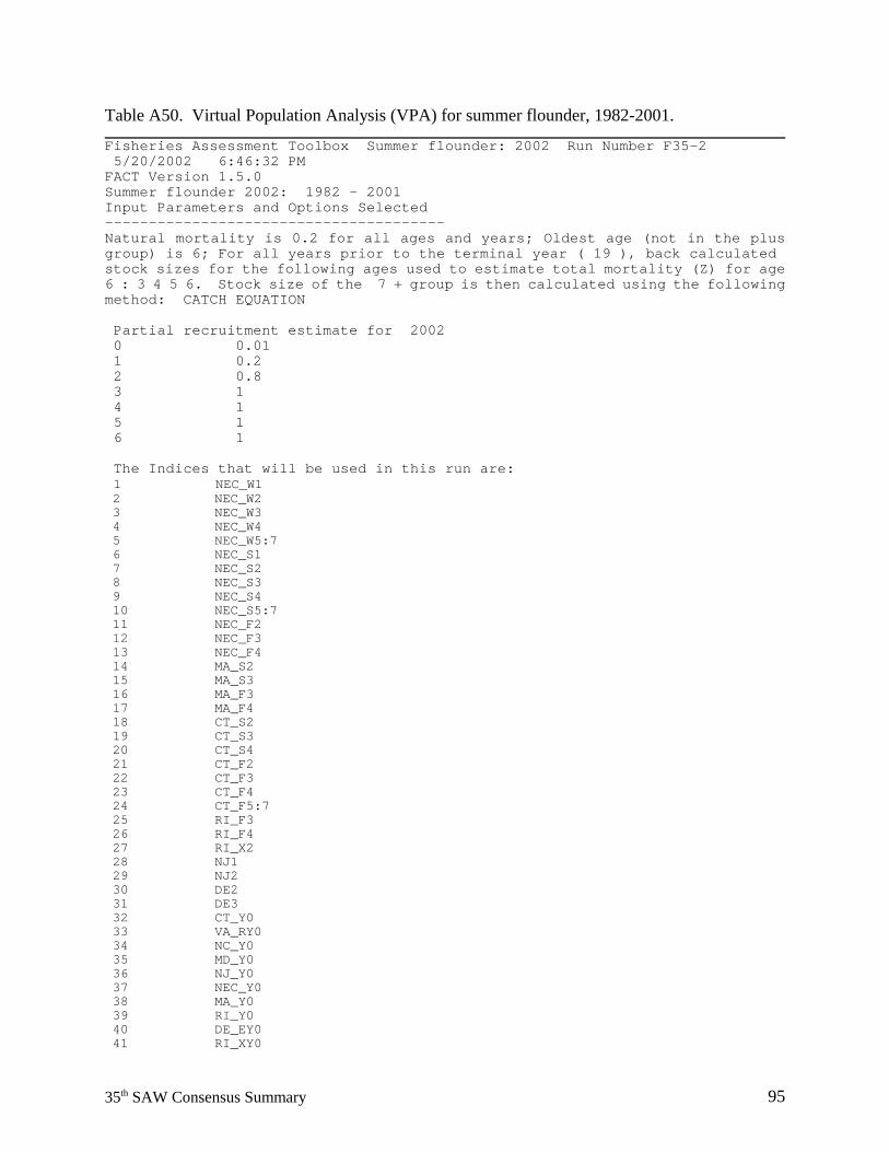
9535th SAW Consensus Summary
Table A50. Virtual Population Analysis (VPA) for summer flounder, 1982-2001.
Fisheries Assessment Toolbox Summer flounder: 2002 Run Number F35-2 5/20/2002 6:46:32 PM FACT Version 1.5.0Summer flounder 2002: 1982 - 2001 Input Parameters and Options Selected---------------------------------------Natural mortality is 0.2 for all ages and years; Oldest age (not in the plusgroup) is 6; For all years prior to the terminal year ( 19 ), back calculated stock sizes for the following ages used to estimate total mortality (Z) for age6 : 3 4 5 6. Stock size of the 7 + group is then calculated using the followingmethod: CATCH EQUATION
Partial recruitment estimate for 2002 0 0.01 1 0.2 2 0.8 3 1 4 1 5 1 6 1
The Indices that will be used in this run are: 1 NEC_W1 2 NEC_W2 3 NEC_W3 4 NEC_W4 5 NEC_W5:7 6 NEC_S1 7 NEC_S2 8 NEC_S3 9 NEC_S4 10 NEC_S5:7 11 NEC_F2 12 NEC_F3 13 NEC_F4 14 MA_S2 15 MA_S3 16 MA_F3 17 MA_F4 18 CT_S2 19 CT_S3 20 CT_S4 21 CT_F2 22 CT_F3 23 CT_F4 24 CT_F5:7 25 RI_F3 26 RI_F4 27 RI_X2 28 NJ1 29 NJ2 30 DE2 31 DE3 32 CT_Y0 33 VA_RY0 34 NC_Y0 35 MD_Y0 36 NJ_Y0 37 NEC_Y0 38 MA_Y0 39 RI_Y0 40 DE_EY0 41 RI_XY0
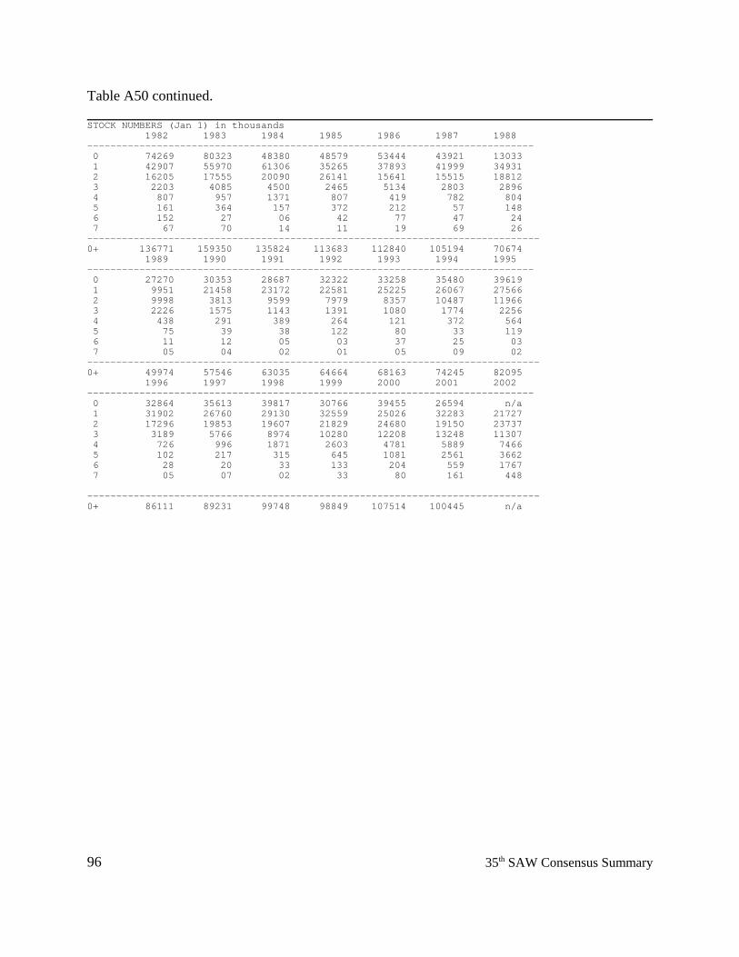
96 35th SAW Consensus Summary
Table A50 continued.
STOCK NUMBERS (Jan 1) in thousands 1982 1983 1984 1985 1986 1987 1988 ----------------------------------------------------------------------------- 0 74269 80323 48380 48579 53444 43921 13033 1 42907 55970 61306 35265 37893 41999 34931 2 16205 17555 20090 26141 15641 15515 18812 3 2203 4085 4500 2465 5134 2803 2896 4 807 957 1371 807 419 782 804 5 161 364 157 372 212 57 148 6 152 27 06 42 77 47 24 7 67 70 14 11 19 69 26------------------------------------------------------------------------------0+ 136771 159350 135824 113683 112840 105194 70674 1989 1990 1991 1992 1993 1994 1995 ----------------------------------------------------------------------------- 0 27270 30353 28687 32322 33258 35480 39619 1 9951 21458 23172 22581 25225 26067 27566 2 9998 3813 9599 7979 8357 10487 11966 3 2226 1575 1143 1391 1080 1774 2256 4 438 291 389 264 121 372 564 5 75 39 38 122 80 33 119 6 11 12 05 03 37 25 03 7 05 04 02 01 05 09 02------------------------------------------------------------------------------0+ 49974 57546 63035 64664 68163 74245 82095 1996 1997 1998 1999 2000 2001 2002 ----------------------------------------------------------------------------- 0 32864 35613 39817 30766 39455 26594 n/a 1 31902 26760 29130 32559 25026 32283 21727 2 17296 19853 19607 21829 24680 19150 23737 3 3189 5766 8974 10280 12208 13248 11307 4 726 996 1871 2603 4781 5889 7466 5 102 217 315 645 1081 2561 3662 6 28 20 33 133 204 559 1767 7 05 07 02 33 80 161 448
------------------------------------------------------------------------------0+ 86111 89231 99748 98849 107514 100445 n/a
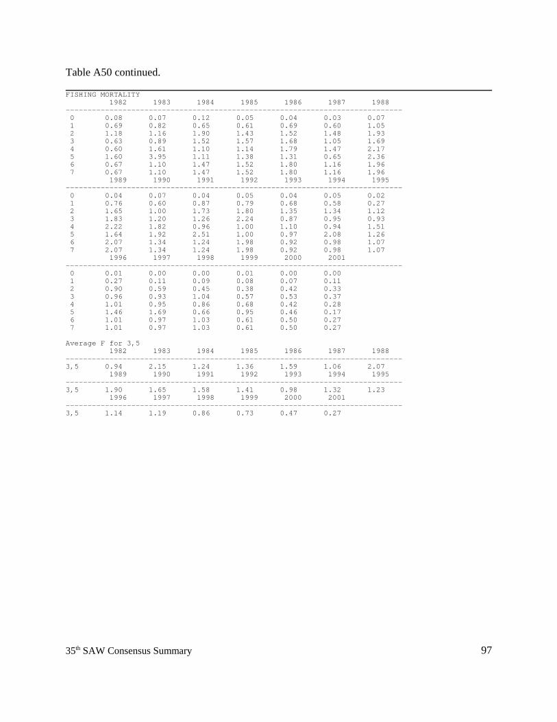
9735th SAW Consensus Summary
Table A50 continued.
FISHING MORTALITY 1982 1983 1984 1985 1986 1987 1988 ----------------------------------------------------------------------------- 0 0.08 0.07 0.12 0.05 0.04 0.03 0.07 1 0.69 0.82 0.65 0.61 0.69 0.60 1.05 2 1.18 1.16 1.90 1.43 1.52 1.48 1.93 3 0.63 0.89 1.52 1.57 1.68 1.05 1.69 4 0.60 1.61 1.10 1.14 1.79 1.47 2.17 5 1.60 3.95 1.11 1.38 1.31 0.65 2.36 6 0.67 1.10 1.47 1.52 1.80 1.16 1.96 7 0.67 1.10 1.47 1.52 1.80 1.16 1.96 1989 1990 1991 1992 1993 1994 1995 ----------------------------------------------------------------------------- 0 0.04 0.07 0.04 0.05 0.04 0.05 0.02 1 0.76 0.60 0.87 0.79 0.68 0.58 0.27 2 1.65 1.00 1.73 1.80 1.35 1.34 1.12 3 1.83 1.20 1.26 2.24 0.87 0.95 0.93 4 2.22 1.82 0.96 1.00 1.10 0.94 1.51 5 1.64 1.92 2.51 1.00 0.97 2.08 1.26 6 2.07 1.34 1.24 1.98 0.92 0.98 1.07 7 2.07 1.34 1.24 1.98 0.92 0.98 1.07 1996 1997 1998 1999 2000 2001 ----------------------------------------------------------------------------- 0 0.01 0.00 0.00 0.01 0.00 0.00 1 0.27 0.11 0.09 0.08 0.07 0.11 2 0.90 0.59 0.45 0.38 0.42 0.33 3 0.96 0.93 1.04 0.57 0.53 0.37 4 1.01 0.95 0.86 0.68 0.42 0.28 5 1.46 1.69 0.66 0.95 0.46 0.17 6 1.01 0.97 1.03 0.61 0.50 0.27 7 1.01 0.97 1.03 0.61 0.50 0.27
Average F for 3,5 1982 1983 1984 1985 1986 1987 1988 -----------------------------------------------------------------------------3,5 0.94 2.15 1.24 1.36 1.59 1.06 2.07 1989 1990 1991 1992 1993 1994 1995 -----------------------------------------------------------------------------3,5 1.90 1.65 1.58 1.41 0.98 1.32 1.23 1996 1997 1998 1999 2000 2001 -----------------------------------------------------------------------------3,5 1.14 1.19 0.86 0.73 0.47 0.27
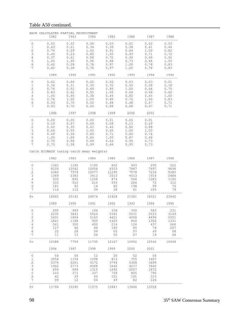
98 35th SAW Consensus Summary
Table A50 continued.
BACK CALCULATED PARTIAL RECRUITMENT 1982 1983 1984 1985 1986 1987 1988 ---------------------------------------------------------------------------- 0 0.05 0.02 0.06 0.03 0.02 0.02 0.03 1 0.43 0.21 0.34 0.39 0.38 0.41 0.44 2 0.74 0.29 1.00 0.91 0.84 1.00 0.82 3 0.40 0.23 0.80 1.00 0.93 0.71 0.72 4 0.37 0.41 0.58 0.72 0.99 0.99 0.92 5 1.00 1.00 0.58 0.88 0.73 0.44 1.00 6 0.42 0.28 0.78 0.97 1.00 0.78 0.83 7 0.42 0.28 0.78 0.97 1.00 0.78 0.83
1989 1990 1991 1992 1993 1994 1995 ---------------------------------------------------------------------------- 0 0.02 0.04 0.02 0.02 0.03 0.03 0.01 1 0.34 0.31 0.35 0.35 0.50 0.28 0.18 2 0.74 0.52 0.69 0.80 1.00 0.64 0.75 3 0.83 0.62 0.50 1.00 0.64 0.46 0.62 4 1.00 0.95 0.38 0.44 0.82 0.45 1.00 5 0.74 1.00 1.00 0.45 0.72 1.00 0.83 6 0.93 0.70 0.50 0.88 0.68 0.47 0.71 7 0.93 0.70 0.50 0.88 0.68 0.47 0.71
1996 1997 1998 1999 2000 2001 ---------------------------------------------------------------------------- 0 0.00 0.00 0.00 0.01 0.00 0.01 1 0.19 0.07 0.09 0.08 0.13 0.29 2 0.62 0.35 0.43 0.40 0.80 0.88 3 0.66 0.55 1.00 0.60 1.00 1.00 4 0.69 0.56 0.83 0.71 0.80 0.74 5 1.00 1.00 0.64 1.00 0.87 0.46 6 0.70 0.58 0.99 0.64 0.95 0.73 7 0.70 0.58 0.99 0.64 0.95 0.73
Catch BIOMASS (using catch mean weights)
1982 1983 1984 1985 1986 1987 1988 ---------------------------------------------------------------------------- 0 1362 1185 1195 602 493 295 252 1 8226 12042 10658 6333 7867 7697 9698 2 6383 7974 10077 11295 7578 7236 9380 3 1369 2383 3413 2013 4513 1914 2484 4 633 895 1268 874 566 1083 1160 5 333 510 210 593 286 72 312 6 181 42 14 82 198 99 76 7 116 112 39 38 61 155 79------------------------------------------------------------------------------0+ 18602 25142 26874 21828 21561 18551 23442
1989 1990 1991 1992 1993 1994 1995 ---------------------------------------------------------------------------- 0 200 469 146 336 340 583 231 1 2235 3841 5024 5341 5531 5533 3149 2 5431 1804 5165 4651 4008 4496 5051 3 1821 1188 900 1425 840 1352 1331 4 541 350 400 214 124 437 668 5 127 66 84 192 85 74 207 6 22 28 09 05 57 49 08 7 11 13 04 05 07 19 04------------------------------------------------------------------------------0+ 10388 7759 11730 12167 10992 12542 10648
1996 1997 1998 1999 2000 2001 ---------------------------------------------------------------------------- 0 54 06 12 26 02 04 1 3554 1154 1098 813 755 1607 2 5376 5201 4172 3748 5368 3699 3 1962 2773 4588 3640 4237 3645 4 656 694 1315 1692 2007 1872 5 143 371 337 728 805 790 6 42 29 50 151 191 315 7 09 12 04 49 82 126------------------------------------------------------------------------------0+ 11794 10240 11575 10847 13446 12058

9935th SAW Consensus Summary
Table A50 continued.
Jan 1 BIOMASS (using Jan 1 mean weights)
1982 1983 1984 1985 1986 1987 1988 ---------------------------------------------------------------------------- 0 14705 15020 9144 11222 10208 8521 3415 1 13687 18190 18882 11497 13717 14028 12086 2 7552 9602 10306 12888 8368 8425 9876 3 3421 3325 3892 2063 4328 2447 2485 4 1738 1292 1741 1084 583 1173 1132 5 468 614 259 691 393 128 324 6 416 71 13 102 212 121 82 7 259 182 55 52 79 244 98
------------------------------------------------------------------------------0+ 42246 48297 44292 39598 37887 35086 29498
1989 1990 1991 1992 1993 1994 1995 ---------------------------------------------------------------------------- 0 3927 6010 2324 5624 6219 10254 13510 1 3791 6416 7415 5894 8703 9723 12046 2 5789 2326 5279 4404 4788 5789 7156 3 1796 1448 1120 1288 1130 1724 1836 4 566 369 566 340 172 651 839 5 149 69 76 270 128 70 279 6 28 33 11 06 102 63 11 7 13 19 05 06 14 32 07
------------------------------------------------------------------------------0+ 16059 16690 16797 17832 21255 28305 35684
1996 1997 1998 1999 2000 2001 ---------------------------------------------------------------------------- 0 9268 4950 8601 2338 908 984 1 14228 10330 9380 10093 6757 6069 2 9565 11336 10607 11766 12513 11911 3 2730 4053 6650 7833 9046 10837 4 927 1149 2002 2895 5221 6820 5 183 404 543 1048 1929 4336 6 72 44 79 340 464 1338 7 15 21 07 117 227 579
------------------------------------------------------------------------------0+ 36987 32287 37868 36431 37064 42875
100 35th SAW Consensus Summary
Table A50 continued.
SSB AT THE START OF THE SPAWNING SEASON -MALES AND FEMALES (MT) (using SSB mean weights)
1982 1983 1984 1985 1986 1987 1988 ------------------------------------------------------------------------------ 0 5668 5854 3507 4341 4207 3574 1251 1 6150 7180 8615 5534 5890 6863 4123 2 2862 3655 2003 3735 2257 2257 1797 3 1596 1774 1130 629 1248 1133 682 4 795 268 697 459 140 380 196 5 101 17 115 230 120 81 44 6 198 23 05 27 48 50 16 7 126 62 14 12 15 79 16------------------------------------------------------------------------------0+ 17497 18833 16086 14968 13926 14418 8124
1989 1990 1991 1992 1993 1994 1995 ------------------------------------------------------------------------------ 0 1767 2323 1296 2450 2726 3882 4905 1 1487 3415 2803 3349 4260 5193 7239 2 1403 1023 1220 1023 1452 1655 2436 3 430 577 402 224 651 927 929 4 87 84 270 136 68 303 224 5 37 14 10 122 56 14 93 6 04 11 04 01 41 32 04 7 02 05 02 01 05 12 02------------------------------------------------------------------------------0+ 5216 7453 6007 7304 9260 12017 15834
1996 1997 1998 1999 2000 2001 ------------------------------------------------------------------------------ 0 3475 2428 3316 1408 1777 872 1 7902 6727 8089 6910 7345 9688 2 3565 5907 6691 7204 9171 8458 3 1311 1962 2760 4879 6159 7967 4 411 472 1021 1806 3791 5760 5 51 102 371 496 1385 4054 6 26 19 31 184 295 976 7 06 08 02 60 127 391------------------------------------------------------------------------------0+ 16746 17625 22280 22948 30050 38166
10135th SAW Consensus Summary
Table A51. VPA Bootstrap results: precision of estimates.
The number of bootstraps: 500 Bootstrap Output Variable: N hat-------------------------------------------------------------------------- NLLS BOOTSTRAP BOOTSTRAP C.V. FOR ESTIMATE MEAN Std Error NLLS SOLNN 1 21727 22185 4399 0.20N 2 23737 24038 4018 0.17N 3 11307 11396 1904 0.17N 4 7466 7510 1213 0.16N 5 3662 3681 798 0.22N 6 1767 1804 471 0.27 NLLS EST C.V. FOR BIAS BIAS PERCENT CORRECTED CORRECTED LOWER UPPER ESTIMATE STD ERROR BIAS FOR BIAS ESTIMATE 80%CI 80%CIN 1 458 197 2.11 21270 0.206828 16216 27505N 2 300 180 1.27 23437 0.171459 19087 29100N 3 90 85 0.79 11217 0.169766 9103 13864N 4 44 54 0.59 7422 0.163492 5895 9064N 5 20 36 0.54 3642 0.219021 2868 4959N 6 37 21 2.10 1730 0.272477 1148 2305
102 35th SAW Consensus Summary
Table A51 continued.Bootstrap Output Variable: F t-------------------------------------------------------------------------- NLLS BOOTSTRAP BOOTSTRAP C.V. FOR ESTIMATE MEAN StdError NLLS SOLNAge 0 0.0021 0.0022 0.0004 0.21Age 1 0.1075 0.1090 0.0177 0.17Age 2 0.3269 0.3316 0.0487 0.15Age 3 0.3735 0.3786 0.0519 0.14Age 4 0.2752 0.2839 0.0544 0.20Age 5 0.1714 0.1788 0.0475 0.28Age 6 0.2734 0.2804 0.0315 0.12Age 7 0.2734 0.2804 0.0315 0.12 NLLS EST C.V. FOR BIAS BIAS PERCENT CORRECTED CORRECTED LOWER UPPER ESTIMATE STD ERROR BIAS FOR BIAS ESTIMATE 80%CI 80%CIAge 0 0.0000396 0.0000197 1.865 0.0020821 0.21 0.0017 0.0028Age 1 0.0014651 0.0007932 1.363 0.1060253 0.17 0.0884 0.1316Age 2 0.0046466 0.0021784 1.421 0.3222752 0.15 0.2726 0.3892Age 3 0.0051271 0.0023231 1.373 0.3683516 0.14 0.3160 0.4516Age 4 0.0086827 0.0024324 3.155 0.2665285 0.20 0.2095 0.3390Age 5 0.0074158 0.0021235 4.327 0.1639547 0.29 0.1335 0.2521Age 6 0.0070752 0.0014103 2.588 0.2662783 0.12 0.2370 0.3162Age 7 0.0070752 0.0014103 2.588 0.2662783 0.12 0.2370 0.3162Bootstrap Output Variable: F full t-------------------------------------------------------------------------- NLLS BOOTSTRAP BOOTSTRAP C.V. FOR ESTIMATE MEAN StdError NLLS SOLN 0.2734 0.2804 0.0315 0.12
NLLS EST C.V. FOR BIAS BIAS PERCENT CORRECTED CORRECTED LOWER UPPER ESTIMATE STD ERROR BIAS FOR BIAS ESTIMATE 80%CI 80%CI 0.00708 0.00141 2.59 0.26628 0.12 0.2370 0.3162
10335th SAW Consensus Summary
Table A51 continued.
Bootstrap Output Variable: SSB spawn t-------------------------------------------------------------------------- NLLS BOOTSTRAP BOOTSTRAP C.V. FOR ESTIMATE MEAN StdError NLLS SOLN 38166.3196 38502.5412 3309.9183 0.09
NLLS EST C.V. FOR BIAS BIAS PERCENT CORRECTED CORRECTED LOWER UPPER ESTIMATE STD ERROR BIAS FOR BIAS ESTIMATE 80%CI 80%CI 336.22 148.02 0.88 37830.10 0.09 34164.5520 42579.9361
Bootstrap Output Variable: Jan 1 biomass-------------------------------------------------------------------------- NLLS BOOTSTRAP BOOTSTRAP C.V. FOR ESTIMATE MEAN StdError NLLS SOLN 42874.5306 43159.7457 2973.0448 0.07
NLLS EST C.V. FOR BIAS BIAS PERCENT CORRECTED CORRECTED LOWER UPPER ESTIMATE STD ERROR BIAS FOR BIAS ESTIMATE 80%CI 80%CI 285.22 132.96 0.67 42589.32 0.07 39279.15 46922.42
104 35th SAW Consensus Summary
Table A52. VPA Retrospective analysis for summer flounder. Fishing Mortality (F)Terminal 1982 1983 1984 1985 1986 1987 1988 1989 1990 1991 1992 1993 1994 1995 1996 1997 1998 1999 2000 2001 Year 1996 0.94 2.15 1.24 1.36 1.59 1.06 2.07 1.90 1.65 1.58 1.42 0.99 1.37 1.41 1.99 1997 0.94 2.15 1.24 1.36 1.59 1.06 2.07 1.90 1.65 1.58 1.41 0.98 1.33 1.25 1.26 5.99 1998 0.94 2.15 1.24 1.36 1.59 1.06 2.07 1.90 1.65 1.58 1.41 0.98 1.32 1.22 1.09 1.02 0.59 1999 0.94 2.15 1.24 1.36 1.59 1.06 2.07 1.90 1.65 1.58 1.41 0.98 1.32 1.21 1.08 1.03 0.60 0.40 2000 0.94 2.15 1.24 1.36 1.59 1.06 2.07 1.90 1.65 1.58 1.41 0.98 1.32 1.23 1.12 1.12 0.72 0.57 0.36 2001 0.94 2.15 1.24 1.36 1.59 1.06 2.07 1.90 1.65 1.58 1.41 0.98 1.32 1.23 1.14 1.19 0.86 0.73 0.47 0.27
Spawning Stock Biomass (SSB)Terminal 1982 1983 1984 1985 1986 1987 1988 1989 1990 1991 1992 1993 1994 1995 1996 1997 1998 1999 2000 2001 Year 1996 17497 18833 16086 14968 13926 14418 8124 5215 7449 5997 7254 9101 12187 17674 19516 1997 17497 18833 16086 14968 13926 14418 8124 5216 7453 6007 7293 9289 12754 18770 20969 21782 1998 17497 18833 16086 14968 13926 14418 8124 5216 7453 6008 7311 9277 12251 17226 19430 20710 23482 1999 17497 18833 16086 14968 13926 14418 8124 5216 7453 6008 7310 9287 12271 16844 18640 20262 24795 25243 2000 17497 18833 16086 14968 13926 14418 8124 5216 7453 6007 7307 9271 12066 16372 17793 19111 24456 25644 32657 2001 17497 18833 16086 14968 13926 14418 8124 5216 7453 6007 7304 9260 12017 15834 16746 17625 22280 22948 30050 38166
Population numbers: Age-0Terminal 1982 1983 1984 1985 1986 1987 1988 1989 1990 1991 1992 1993 1994 1995 1996 1997 1998 1999 2000 2001 Year 1996 74269 80323 48380 48579 53444 43920 13031 27269 30329 28630 32028 32749 39614 48642 30368 1997 74269 80323 48380 48579 53444 43922 13033 27270 30361 28663 32213 33965 40689 50289 29383 21451 1998 74269 80323 48380 48579 53444 43921 13033 27270 30354 28697 32370 33269 37292 46534 35898 25251 26377 1999 74269 80323 48380 48579 53444 43921 13033 27270 30356 28697 32351 33429 37139 43414 35712 34444 30853 26064 2000 74269 80323 48380 48579 53444 43921 13033 27270 30354 28689 32343 33318 35689 43181 33101 37245 40276 27233 35822 2001 74269 80323 48380 48579 53444 43921 13033 27270 30353 28687 32322 33258 35480 39619 32864 35613 39817 30766 39455 26594
10535th SAW Consensus Summary
Table A53. Input parameters and short term stochastic projection results for summer flounder. Starting stock sizes on January 1, 2002are as estimated by VPA bootstrap procedure. Age-0 recruitment levels in 2002-2004 are estimated as the median of 500 randomestimates selected from VPA estimated numbers at age 0 (000s) during 1982-2001. Fishing mortality was apportioned amonglandings and discard based on the proportion of F associated with landings and discards at age during 1999-2001. Mean weightsat age (landings and discards) are weighted (by fishery) geometric means of 1999-2001 values. Total stock biomass is the productof January 1 numbers at age and January 1 mean weights at age estimated from total catch (landings plus discards) weights. Proportion of F and M before spawning = 0.83 (spawning peak at 1 November).
Age MedianStock Size
in 2002
FishingMortalityPattern
ProportionLanded
ProportionMature
Mean WeightsJanuary 1
Total Biomass
Mean WeightsLandings
Mean WeightsDiscards
0 35613 0.01 0.00 0.38 0.040 0.144 0.0931 23156 0.18 0.43 0.72 0.251 0.536 0.4252 26637 0.78 0.75 0.90 0.554 0.709 0.5863 12957 1.00 0.90 1.00 0.773 0.933 0.8904 6741 1.00 0.97 1.00 1.120 1.403 1.3865 2861 1.00 0.97 1.00 1.700 2.103 2.0996 2083 1.00 0.97 1.00 2.405 2.655 2.410
7+ 395 1.00 0.97 1.00 3.291 3.135 2.972
2002 Landings = 10,991 mt; 2002-2004 median recruitment from 1982-2001 VPA estimates (35.6 million)
Forecast medians (50% probability level) (landings, discards, and total stock biomass (B) in '000 mt)
2002 2003 2004 F Land. Disc. B F Land. Disc. B F Land. Disc. B
0.32 11.0 1.7 51.4 0.26 10.6 1.5 57.6 0.26 12.2 1.7 65.6
106 35th SAW Consensus Summary
1980
1985
1990
1995
2000
-1 0 1 2 3 4 5 6 7 8
Year
Summer flounderTotal Catch Age Composition
AgeFigure A1. Total catch age composition for summer flounder: 1982-2001
10735th SAW Consensus Summary
Year1982 1984 1986 1988 1990 1992 1994 1996 1998 2000 2002
Mea
n w
eigh
t (kg
)
0
1
2
3
4
5
Figure A2. Trends in mean weight at age in the total catch of summer flounder.
Age 0
Age 1Age 2Age 3
Age 4
Age 5Age 6
Age 7+
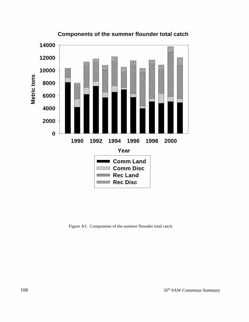
108 35th SAW Consensus Summary
Year1990 1992 1994 1996 1998 2000
Met
ric to
ns
0
2000
4000
6000
8000
10000
12000
14000
Comm Land Comm Disc Rec Land Rec Disc
Components of the summer flounder total catch
Figure A3. Components of the summer flounder total catch.
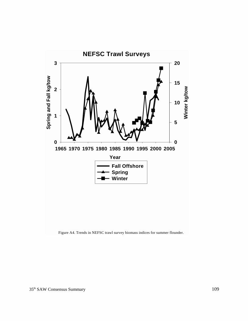
10935th SAW Consensus Summary
NEFSC Trawl Surveys
Year1965 1970 1975 1980 1985 1990 1995 2000 2005
Sprin
g an
d Fa
ll kg
/tow
0
1
2
3
Win
ter k
g/to
w
0
5
10
15
20
Fall Offshore Spring Winter
Figure A4. Trends in NEFSC trawl survey biomass indices for summer flounder.
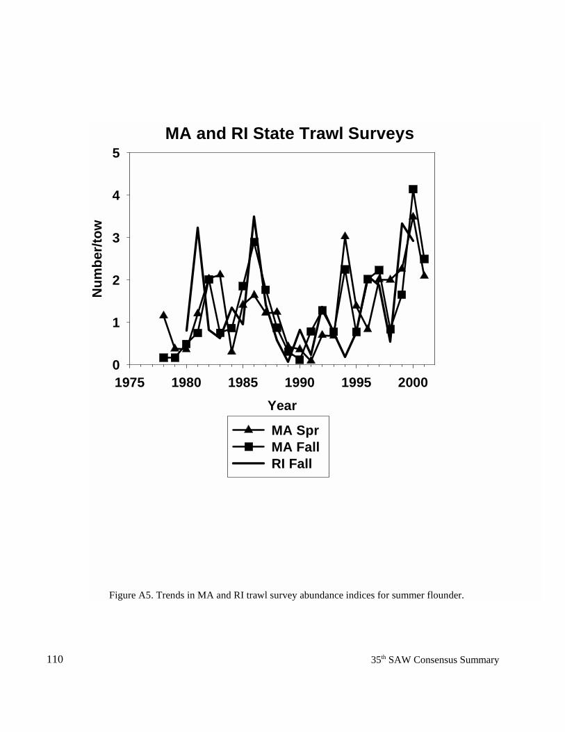
110 35th SAW Consensus Summary
MA and RI State Trawl Surveys
Year1975 1980 1985 1990 1995 2000
Num
ber/t
ow
0
1
2
3
4
5
MA Spr MA Fall RI Fall
Figure A5. Trends in MA and RI trawl survey abundance indices for summer flounder.
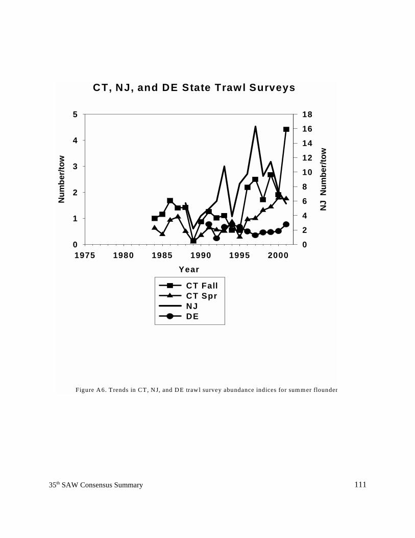
11135th SAW Consensus Summary
CT, NJ, and DE State Trawl Surveys
Year1975 1980 1985 1990 1995 2000
Num
ber/t
ow
0
1
2
3
4
5
NJ
Num
ber/t
ow
024681012141618
CT Fall CT Spr NJ DE
Figure A6. Trends in CT, NJ, and DE trawl survey abundance indices for summer flounder
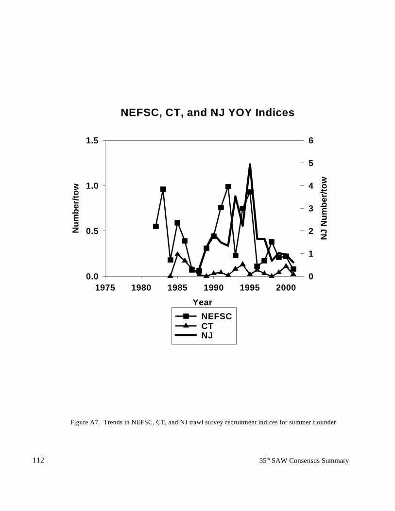
112 35th SAW Consensus Summary
NEFSC, CT, and NJ YOY Indices
Year1975 1980 1985 1990 1995 2000
Num
ber/t
ow
0.0
0.5
1.0
1.5
NJ
Num
ber/t
ow
0
1
2
3
4
5
6
NEFSCCTNJ
Figure A7. Trends in NEFSC, CT, and NJ trawl survey recruitment indices for summer flounder
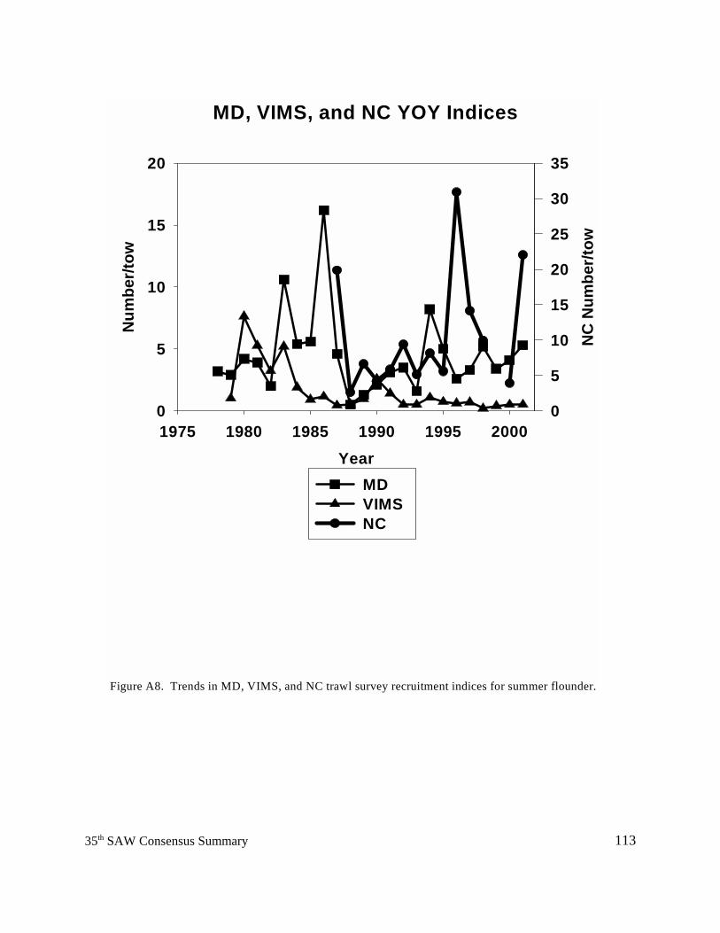
11335th SAW Consensus Summary
MD, VIMS, and NC YOY Indices
Year1975 1980 1985 1990 1995 2000
Num
ber/t
ow
0
5
10
15
20
NC
Num
ber/t
ow
0
5
10
15
20
25
30
35
MDVIMS NC
Figure A8. Trends in MD, VIMS, and NC trawl survey recruitment indices for summer flounder.
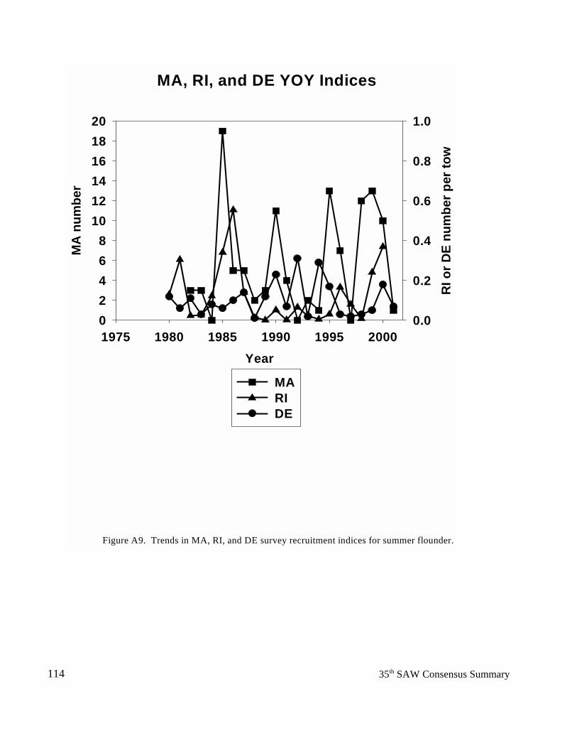
114 35th SAW Consensus Summary
MA, RI, and DE YOY Indices
Year1975 1980 1985 1990 1995 2000
MA
num
ber
02468
101214161820
RI o
r DE
num
ber p
er to
w
0.0
0.2
0.4
0.6
0.8
1.0
MARI DE
Figure A9. Trends in MA, RI, and DE survey recruitment indices for summer flounder.
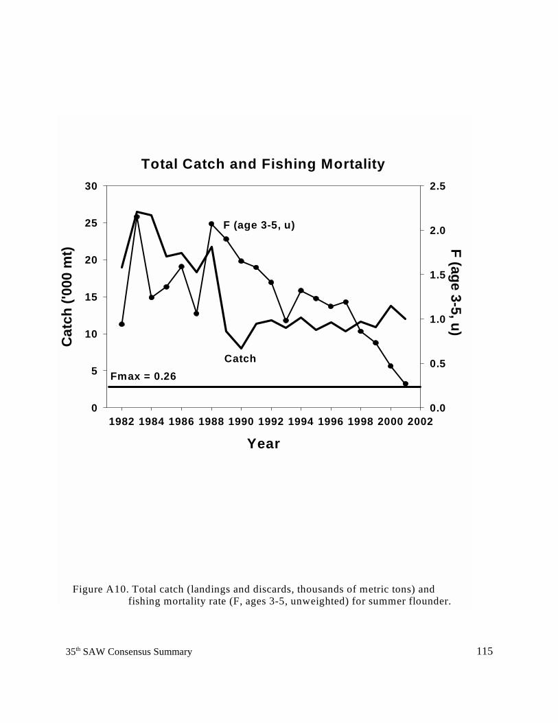
11535th SAW Consensus Summary
Year1982 1984 1986 1988 1990 1992 1994 1996 1998 2000 2002
Cat
ch ('
000
mt)
0
5
10
15
20
25
30
F (age 3-5, u)
0.0
0.5
1.0
1.5
2.0
2.5
Total Catch and Fishing Mortality
Catch
F (age 3-5, u)
Fmax = 0.26
Figure A10. Total catch (landings and discards, thousands of metric tons) and fishing mortality rate (F, ages 3-5, unweighted) for summer flounder.
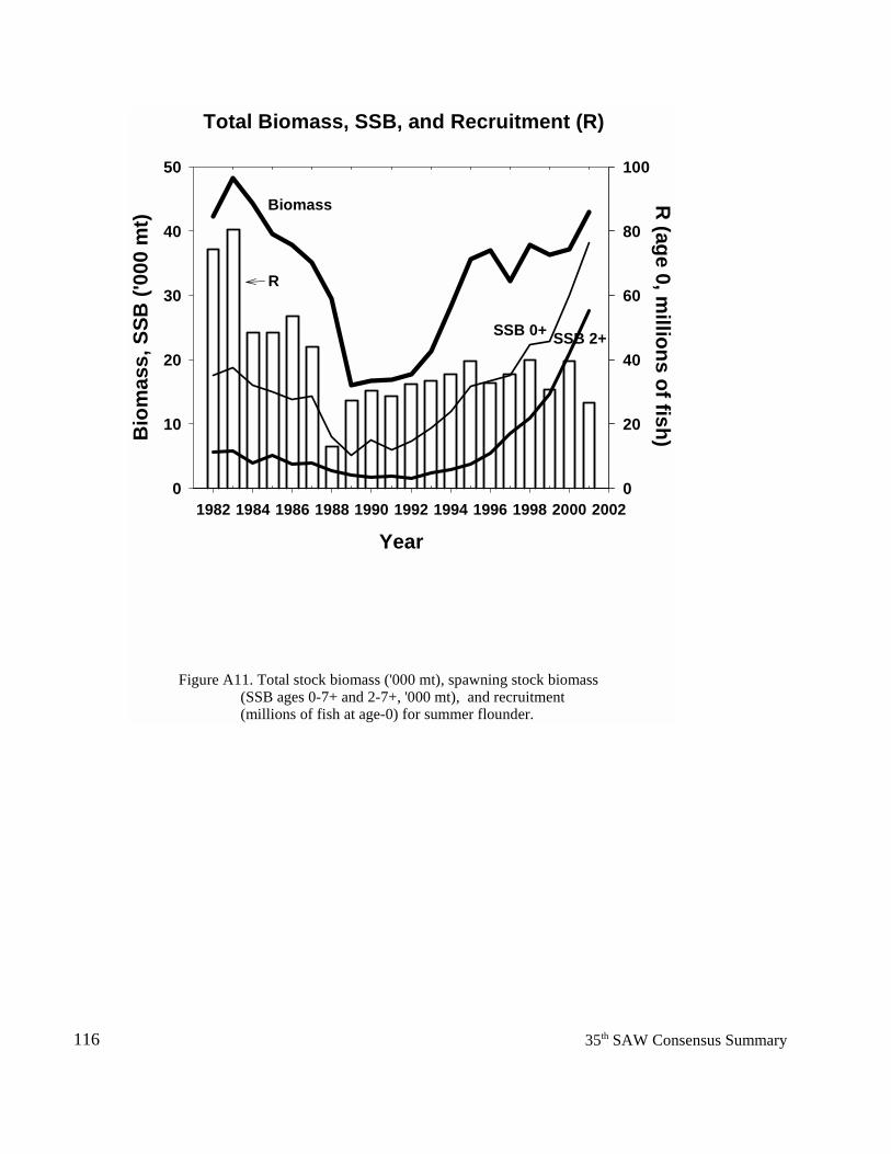
116 35th SAW Consensus Summary
Year1982 1984 1986 1988 1990 1992 1994 1996 1998 2000 2002
Bio
mas
s, S
SB ('
000
mt)
0
10
20
30
40
50
R (age 0, m
illions of fish)
0
20
40
60
80
100
Total Biomass, SSB, and Recruitment (R)
Biomass
SSB 0+ SSB 2+
R
Figure A11. Total stock biomass ('000 mt), spawning stock biomass (SSB ages 0-7+ and 2-7+, '000 mt), and recruitment (millions of fish at age-0) for summer flounder.
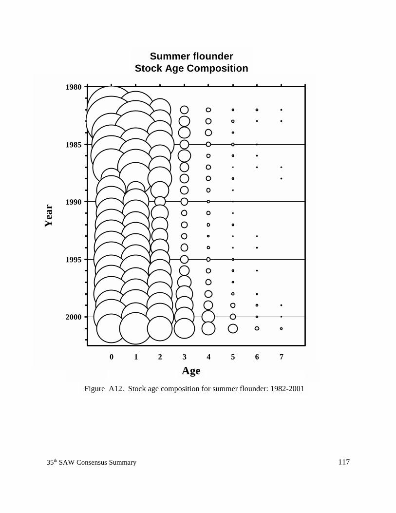
11735th SAW Consensus Summary
1980
1985
1990
1995
2000
-1 0 1 2 3 4 5 6 7 8
Yea
rSummer flounder
Stock Age Composition
AgeFigure A12. Stock age composition for summer flounder: 1982-2001
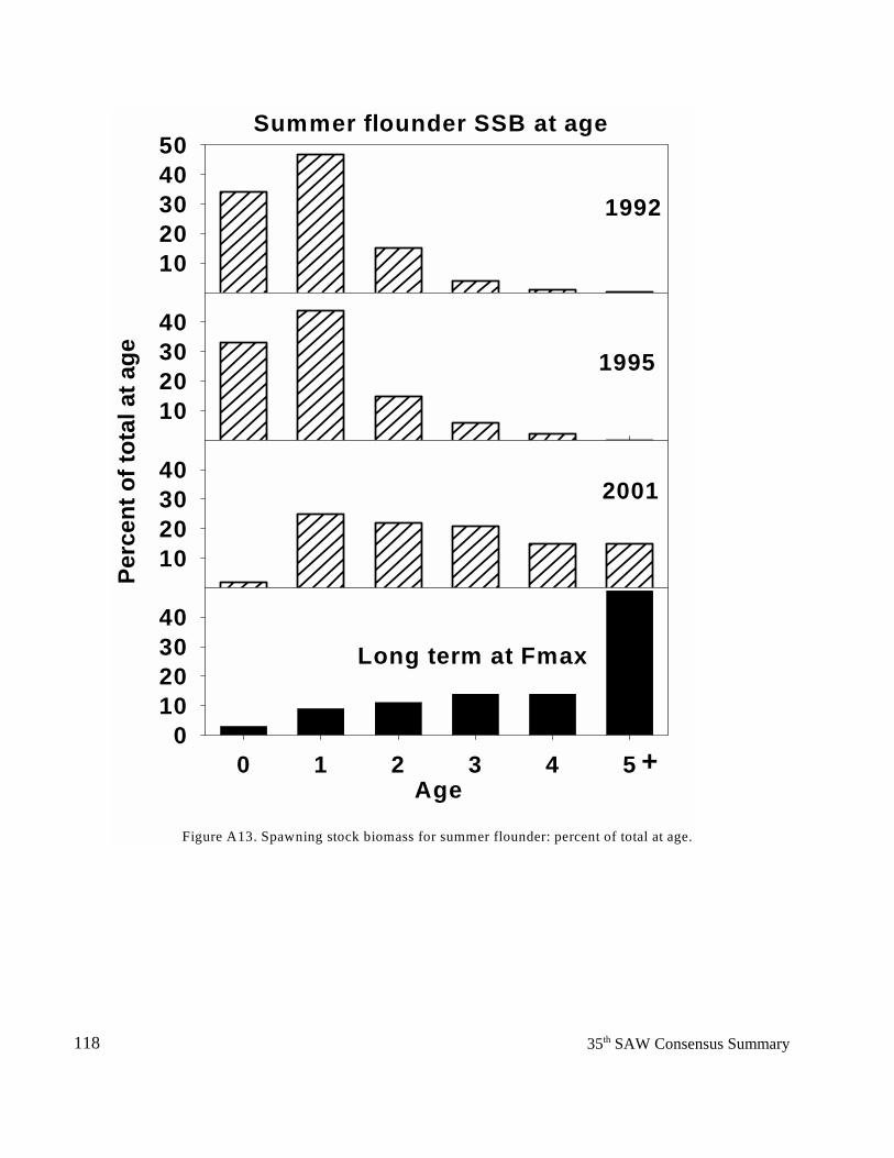
118 35th SAW Consensus Summary
1020304050
1992
Perc
ent o
f tot
al a
t age
10203040
1995
10203040
2001
Age0 1 2 3 4 5
010203040
Long term at Fmax
+
Figure A13. Spawning stock biomass for summer flounder: percent of total at age.
Summer flounder SSB at age
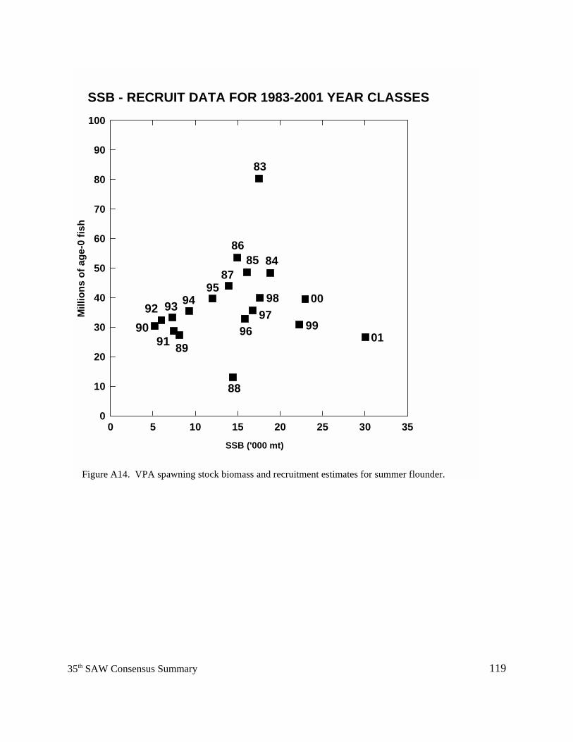
11935th SAW Consensus Summary
0 5 10 15 20 25 30 350
10
20
30
40
50
60
70
80
90
100
93
SSB - RECRUIT DATA FOR 1983-2001 YEAR CLASSES
91
9290
SSB ('000 mt)
86
8785 84
88
89
83
9495
9796
98
Figure A14. VPA spawning stock biomass and recruitment estimates for summer flounder.
99
Mill
ions
of a
ge-0
fish
00
01
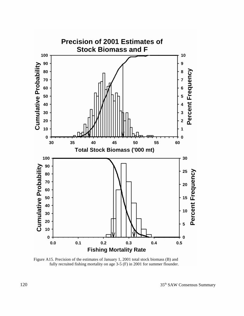
120 35th SAW Consensus Summary
Total Stock Biomass ('000 mt)30 35 40 45 50 55 60
Cum
ulat
ive
Prob
abili
ty
0
10
20
30
40
50
60
70
80
90
100
Perc
ent F
requ
ency
0
1
2
3
4
5
6
7
8
9
10
Precision of 2001 Estimates of Stock Biomass and F
Fishing Mortality Rate0.0 0.1 0.2 0.3 0.4 0.5
Cum
ulat
ive
Prob
abili
ty
0
10
20
30
40
50
60
70
80
90
100
Perc
ent F
requ
ency
0
5
10
15
20
25
30
Figure A15. Precision of the estimates of January 1, 2001 total stock biomass (B) and fully recruited fishing mortality on age 3-5 (F) in 2001 for summer flounder.
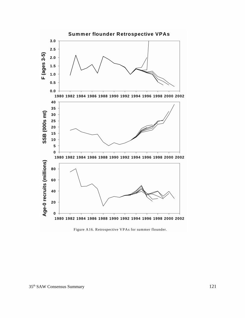
12135th SAW Consensus Summary
1980 1982 1984 1986 1988 1990 1992 1994 1996 1998 2000 2002
F (a
ges
3-5)
0.0
0.5
1.0
1.5
2.0
2.5
3.0Summer flounder Retrospective VPAs
1980 1982 1984 1986 1988 1990 1992 1994 1996 1998 2000 2002
SSB
(000
s m
t)
05
10152025303540
1980 1982 1984 1986 1988 1990 1992 1994 1996 1998 2000 2002
Age
-0 re
crui
ts (m
illio
ns)
0
20
40
60
80
Figure A16. Retrospective VPAs for summer flounder.
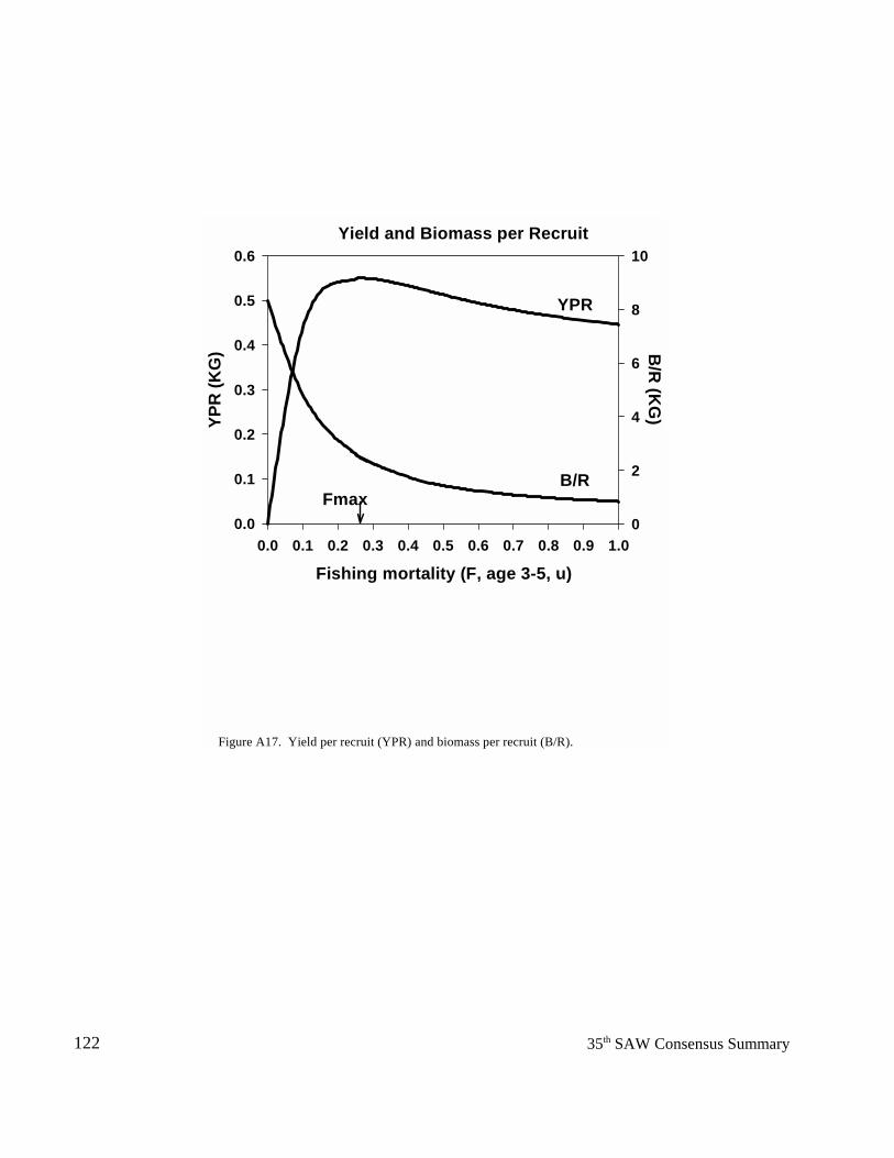
122 35th SAW Consensus Summary
Fishing mortality (F, age 3-5, u)0.0 0.1 0.2 0.3 0.4 0.5 0.6 0.7 0.8 0.9 1.0
YPR
(KG
)
0.0
0.1
0.2
0.3
0.4
0.5
0.6B
/R (K
G)
0
2
4
6
8
10Yield and Biomass per Recruit
YPR
B/RFmax
Figure A17. Yield per recruit (YPR) and biomass per recruit (B/R).
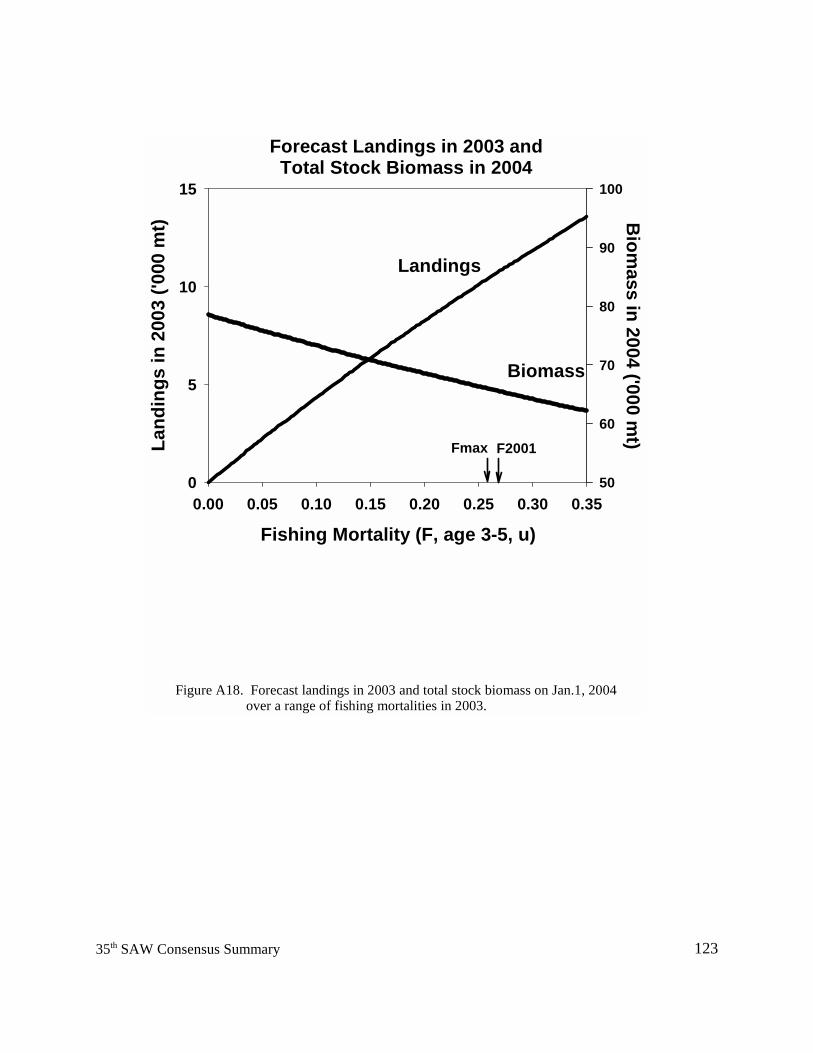
12335th SAW Consensus Summary
Fishing Mortality (F, age 3-5, u)0.00 0.05 0.10 0.15 0.20 0.25 0.30 0.35
Land
ings
in 2
003
('000
mt)
0
5
10
15B
iomass in 2004 ('000 m
t)
50
60
70
80
90
100
Forecast Landings in 2003 and Total Stock Biomass in 2004
Landings
Biomass
Fmax F2001
Figure A18. Forecast landings in 2003 and total stock biomass on Jan.1, 2004 over a range of fishing mortalities in 2003.
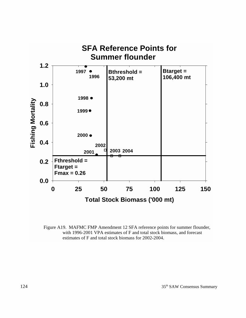
124 35th SAW Consensus Summary
SFA Reference Points for Summer flounder
Total Stock Biomass ('000 mt)0 25 50 75 100 125 150
Fish
ing
Mor
talit
y
0.0
0.2
0.4
0.6
0.8
1.0
1.2
Fthreshold = Ftarget = Fmax = 0.26
Bthreshold = 53,200 mt
Btarget = 106,400 mt1996
1997
1998
1999
2000
20012002
Figure A19. MAFMC FMP Amendment 12 SFA reference points for summer flounder, with 1996-2001 VPA estimates of F and total stock biomass, and forecast estimates of F and total stock biomass for 2002-2004.
2003 2004
35th SAW Consensus Summary 125
B. SCUP
TERMS OF REFERENCE 1. Characterize the commercial and recreational catch including landings and discards. 2. Estimate fishing mortality, spawning stock biomass, and total stock biomass for the current year and characterize the uncertainty of those estimates. 3. Evaluate and either update or re-estimate biological reference points as appropriate. 4. Where appropriate, estimate a TAC and/or TAL based on stock status and target mortality rate for the year following the terminal assessment year. 5. If stock projections are possible, provide short term projections (2-3 years) of stock status under various TAC/F strategies and evaluate current and projected stock status against existing rebuilding or recovery schedules, as appropriate.
INTRODUCTION
Scup, Stenotomus chrysops, are a schooling, continental shelf species of the Northwest Atlantic, distributed primarily between Cape Cod, MA and Cape Hatteras, NC (Morse 1978). Scup undertake extensive migrations between coastal waters in summer and offshore waters in winter. Scup migrate north and inshore to spawn in spring. Larger scup (0.7-1.8 kg) tend to arrive in spring first, followed by smaller scup (Neville and Talbot 1964; Sisson 1974). Larger scup are found during summer near the mouth of larger bays and in the ocean within the 20-fathom contour; smaller scup are found in shallow areas of bays (Morse 1978). Scup migrate south and offshore in autumn as the water temperature decreases, arriving in offshore wintering areas by December (Hamer 1970; Morse 1978).
Spawning occurs from May through August and peaks in June. About 50% of age-2 scup are sexually mature (about 17 cm total length; NEFSC 1993). Scup can attain a maximum length of about 40 cm and a maximum age of about 20 years (Dery and Rearden 1979). Crecco et al. (1981) have characterized scup as slow-growing and relatively long-lived fish.
Tagging studies (e.g., Neville and Talbot 1964; Cogswell 1960, 1961; Hamer 1970, 1979)
have indicated the possibility of two stocks of scup, one in Southern New England and another extending south from New Jersey. However, a lack of definitive tag return data coupled with distributional data from the NEFSC bottom trawl surveys support the concept of a single unit stock extending from Cape Hatteras north to New England (Mayo 1982).
35th SAW Consensus Summary 126
The Mid-Atlantic Fishery Management Council (MAFMC) and the Atlantic States Marine Fisheries Commission (ASMFC) manage scup under Amendment 8 to the Summer Flounder, Scup, and Black Sea Bass Fishery Management Plan (FMP). The FMP defines the management unit as scup in US waters from Cape Hatteras northward to the US-Canadian border. Exploitation rates were to be reduced to 47% (F=0.72) in 1997-1999, to 33% (F=0.45) in 2000-2001, and to 21% (F=0.26) in 2002 through coast-wide commercial quotas and recreational season, size and possession limits that are established on an annual basis. Amendment 12 to the FMP established a biomass threshold for scup based on the maximum value of the 3-year moving average of the NEFSC spring bottom trawl survey index of spawning stock biomass - 2.77 kg per tow, 1977-1979. The scup stock is overfished when the spawning stock biomass index falls below this value. Amendment 12 defined overfishing for scup to occur when the fishing mortality rate exceeds the threshold fishing mortality of Fmax=0.26.
The Total Allowable Catch (TAC) of 9.11 million lbs (4,132 mt) established in 1997
included a commercial fishery quota of 6.00 million lbs (2,722 mt), a recreational fishery harvest limit of 1.95 million lbs (885 mt), and projected total discards of 1.16 million lbs (528 mt). The TAC decreased steadily to a low of 5.92 million lbs in 1999 and 2000 followed by a significant increase in 2001 to 8.37 million lbs (3797 mt). The 2002 TAC increased further to 12.92 million lbs with a commercial quota of 8 million lbs (3629 mt), a recreational harvest limit of 2.77 million lbs (1257 mt) and projected total discards of 2.15 million pounds (975 mt).
For 2002, the Board and Council implemented minimum mesh size regulations that vary according to net size. Large nets may have up to 25 meshes of 4.5@ in the codend, with at least 100 meshes of 5@ forward of the 4.5@ mesh. Small nets, defined as those with codends smaller than 125 meshes including extension, must have 4.5@ mesh throughout. Vessels using nets with smaller mesh may possess 500 lbs. of scup from November through April and 100 lbs. from May through October. The minimum size for scup caught by any net in the commercial fishery remains at 9@.
The ASMFC Summer Flounder, Scup, and Black Sea Bass Management Board approved Addenda V and VII on February 21, 2002 to more effectively manage the scup fishery. Addendum V was enacted to set state-by-state summer period allocations for the summer period scup fishery during 2002 and until action is taken to modify them. The quota was reallocated using 1983-1992 as the base period with updated landings data from Massachusetts.
Addendum VII was implemented to create a state-by-state conservation equivalency system
for the 2002 scup recreational fishery. Under this addendum, each state from North Carolina through New Jersey (inclusive) was assigned size, bag and season regulations, while those states from Massachusetts through New York (inclusive) were required to modify their fishing effort based on the performance of their regulations in previous years. Calculations of the state specific effort necessary to achieve the 2002 harvest limit were based on the average number of fish landed from 1998-2000. The addendum also permitted individual states to separate the management of the Party and Charter Boat sector from the remainder of the recreational fishery, provided that the estimated landings for each mode had a percent standard error not greater than 30%.
35th SAW Consensus Summary 127
THE FISHERY
Commercial Landings US commercial landings averaged over 18,000 mt per year from 1950 to 1966 (peaking at over 22,000 mt in 1960) and declined to about 4,000 mt per year in the early 1970s (Figure B1). Landings fluctuated between 7,000 and 10,000 mt from 1974 to 1986 and have since declined to less than 2,000 mt. Landings in 2001 were 1,729 mt (3.8 million pounds) - less than 8% of the 48.5 million pound peak observed in 1960 (Table B1).
Dealers reported commercial landings in 1994-2001 by market category and not by area of catch. Procedures developed by Wigley et al. (1997) were used to allocate landings by market category to statistical area, based on information collected under the Vessel Trip Report (VTR) system. A monthly set of landings, which are reported in both dealer and VTR databases, are used to characterize the distribution of dealer-reported landings by statistical area. This prorating procedure contributes to uncertainty in the attribution of market category landings by area, especially if vessels that are not participating in any fishery with mandatory VTR requirements land scup from different areas than those that produce landings for participating vessels. Other sources of uncertainty include unreported landings by dealers.
About two-thirds of the commercial landings of scup for the period 1979-2001 were in Rhode Island (37%) and New Jersey (28%) (Table B2). Landings in New York composed an average of 15% of the total. Scup landings reported for Massachusetts were revised for the 31st SARC assessment for 1986-1996, increasing an average of 92% or 218 mt per year (range, 182 to 268 mt and 40 to 216%) (NEFSC 2000). MADMF staff obtained affidavits from several major scup dealers detailing previously unreported landings of scup in Massachusetts for the years 1986-1997. Most of this increase was from previously unreported landings in the hand-line gear category, generally employed from vessels of displacement less than 5 gross registered tons. These records are now included in the NMFS NER dealer landings database.
The otter trawl is the principal commercial fishing gear, accounting for an average of 74% of the total catch in 1979-2001 (Table B3). The remainder of the commercial landings is taken by floating trap (12%) and hand lines (6%), with paired trawl, pound nets, and pots and traps each contributing 2-3%.
The intensity of NER commercial fishery biological sampling in 1979-2001 is summarized in Table B4. Annual sampling intensity varied from 25-640 mt per 100 lengths. Overall sampling exceeded the informal criterion of 100 lengths sampled per 200 mt in 17 of the last 23 years. However, this alone does not indicate adequate sampling because many of these strata have substantial landings but lack samples. Commercial landings at age were not estimated for 1998-2001 because an analytical assessment was determined to be unreliable by SAW 27 (NEFSC 1998) due to concerns about commercial landings sampling and estimation of commercial discards in recent years. Estimation of commercial landings at length using the available sample data indicated that most fish in the 1997-2001 commercial landings were age-3 fish of their respective year classes (Figures B2, B3).
35th SAW Consensus Summary 128
Commercial Discards Estimates
The NEFSC sea sampling program has collected information on landings and discards in the commercial fishery for 1989-2001. NER discard estimates were raised to account for North Carolina landings. A discard mortality rate of 100% was assumed because there are no published estimates of scup discard mortality rates. This assumption is based on limited observations and is a point of some contention between scientists and fishermen. Past SAW panels have recommended that research be conducted to better characterize the mortality of scup in different gear types in order to more accurately assess discard mortality (NEFSC 1995, 1997, 1998, 2000). The number of trips in which scup were landed and/or discarded is tabulated in Table B5. The NEFSC sea sampling program sampled from 7 to 91 otter trawl trips per year in which scup were landed or discarded. The number of sampled trips was especially low in 1994 and 1995 when only 7 and 18 otter trawl trips were sampled. Sample size in 2000 (72 trips) was the largest since 1992, but the number dropped to 28 sampled trips in 2001 (Table B5).
Quantifying discards from the commercial fishery is necessary for a reliable stock assessment, but low sample sizes have resulted in questionable estimates. Concern regarding the poorly estimated discards due to inadequate sampling has been addressed in at least four previous SAW meetings (NEFSC 1995, 1997, 1998, 2000). Members of these previous SARC panels commented that the uncertainty associated with the discards prevents reliable estimates of discard at age in the commercial fishery and seriously impedes the development of a reliable analytic assessment as well as forecasts of catch and stock biomass for the stock. Previous SAW panels have given recommendations for significant improvement in the precision of discard estimates. The most recent SARC that evaluated scup was especially concerned and did not consider an analytical assessment due to uncertainties in the input data, especially discard estimates (NEFSC 2000). Despite the uncertainty of the discard data, the SAW 31 panel concluded that the limited available information suggested that discarding of scup has been high throughout the time series (1989-1999), approaching or exceeding landings. The panel stated that continued unreliability in discard estimates would prevent the use of VPA and production models for producing a reliable assessment.
Given the difficulty associated with estimating commercial discards for scup, the sub-committee considered three different approaches for calculating estimates: 1. Geometric Mean Discards-to-Landings Ratio (GMDL): In previous assessments (e.g., SAW 25
(NEFSC 1997)), ratios of discards to landings by landings level (for trip landings < 300 kg (661 lbs) or => 300 kg) and half year were calculated (uncorrected geometric mean by cell) and multiplied by corresponding observed landings levels from the weigh-out database to provide estimates of discards for use as guidance in setting TAC levels for management (Table B6). Only trips with both non-zero landings and discards could be used. Geometric mean rates (retransformed, mean ln-transformed D/L per trip) were used because the distributions of landings and discards and the ratio of discards to landings on a per-trip basis in the scup fishery are highly variable and positively skewed. N is the number of sea sample trips with both scup landings and discard, which were used to calculate the per trip discard to
35th SAW Consensus Summary 129
landings ratios. Corresponding dealer landings are from the NEFSC database.
The number of trawl gear trips used to calculate geometric mean discard-to-landings ratios (GMDL) by half year for 1997-2001 ranged from 1 to 17 for trips < 300 kg and from 1 to 4 for trips => 300 kg (Table B6). No trawl gear trips were available for half year two in 1997 and 1999 for trips < 300 kg and for half year two in 1997-2001 for trips => 300 kg. The GMDL calculated for half year one was used to estimate discards for half year two when no trawl gear trips were available in half year two. The GMDL ratios ranged from 0.46 in 2001 (half year two, trips < 300 kg) to 121.71 in 1998 (half year one, trips => 300 kg). The large 1998 estimate was based on one trawl gear trip. About 93% of the discard from that trip was attributable to a single tow in which an estimated 68.2 mt (150,000 lbs.) of scup were captured. This tow was not lifted from the water and the captain from the vessel estimated the weight. There has been debate concerning the validity of the tow weight estimate and whether or not it is representative of other vessels in the fishery. However, the observation was reported and was therefore included in the calculation of the GMDL. Estimates for 2001 were relatively low B 0.89 for half year one and 0.46 for half year two for trips < 300 kg (the latter of these was based on only two trawl gear trips) and 0.92 for half year one for trips => 300 kg.
2. Aggregate Discards-to-Landings Ratio (AGDL): The second approach for estimating discards
considered aggregate discards to landings ratios (summed D/summed L for all trips in stratum). As in the GMDL method, trips are stratified by half-year period (HY1, HY2) and trip landings level (< 300 kg, => 300 kg). N is number of sea sample trips in the stratum used to calculate the aggregate ratio (Table B7). The number of trawl gear trips used to calculate AGDL by half year for 1997-2001 ranged from 14 to 37 for trips < 300 kg and from 1 to 4 for trips => 300 kg. There are more trips available for calculation for trips < 300 kg than in the GMDL approach. The lowest AGDL ratio calculated was 0.69 in 2000(half year one, trips => 300 kg). The largest AGDL was 121.71 in 1998 (half year one, trips => 300 kg) B the same as that calculated in the GMDL method.
3. Mean Differences between Landings and Discards (DELTA): Mean differences (kg) between
landings and discard (D = landings - discard, per trip) were also calculated using the same strata as the previous methods - stratified by half-year period (HY1, HY2) and trip landings level (< 300 kg, => 300 kg). N is number of sea sample trips in the stratum used to calculate the mean difference in stratum, which was then applied to the landings of every trip in the NEFSC dealer database to calculate a discard for each trip (discard = landings - (D)). Calculating differences allows use of trips that had discards but no landings, whereas D/L ratios cannot be calculated in these situations (i.e. zero in the denominator). When discards exceed landings, DELTA values will be negative. As the magnitude of discards is of primary interest, the absolute values will be considered.
The number of trawl gear trips used in the DELTA method calculations ranged from 6 to 37
for trips < 300 kg and from 1 to 4 for trips => 300 kg (Table B8). The magnitude of the DELTA
35th SAW Consensus Summary 130
values ranged from 10.7 in 2001 (half year two, trips < 300 kg) to 72707 in 1998 (half year one, trips => 300 kg). As before, this large discarding event is the result of one large discarding event that was discussed above. Comparison of Methods
A summary of landings, discards, and aggregate discards to landings ratios from the three alternative methods of discard calculation are presented in Table B9. The year-to-year trends among the different approaches differed in magnitude but followed similar trends. D/L ratios in 1997 and 2001 were relatively low for all methods within each series. The large discard event in 1998 affected calculations from each method, resulting in relatively high D/L values in 1998 for each approach. The DELTA method yielded estimates that were fairly consistent with the GMDL ratios, while the AGDL estimates exhibited more variability. The working group felt most confident in the estimates produced using the GMDL approach and felt the estimates were supported by the DELTA ratios. The GMDL estimates were used for all modeling approached considered.
Estimates of GMDL from sea sampling were compared to estimates from vessel trip reports (VTR) for 1994-2001 (Table B10). VTR data were selected to include only trawl trips that reported some discard of any species. In contrast to black sea bass and New England groundfish discard data, GM D/L for scup for 1994-2001 sea sample data were 2 to 44 times greater than GM D/L for VTR data, with a single exception in 1996 for trips landing => 300 kg. Length-frequency
The intensity of length frequency sampling of discarded scup from the sea sampling declined in 1992-1995 relative to 1989-1991 (Table B5). Sampling intensity ranged from 496 to 334 mt/100 lengths sampled in 1992-1995, failing to meet the informal criterion of 200 mt/100 lengths sampled. Sampling intensity improved to 100 mt/100 lengths in 1996, but then declined to about 240 mt/100 lengths in 1997 and 1999 and 1,071 mt/100 lengths in 1998. In 2000, sampling intensity dramatically improved to 50 mt/100 lengths. Mean weight was estimated from length frequency data and a length-weight equation, total numbers were estimated by dividing total weight by mean weight, and numbers at length were then calculated from the length-frequency distribution. Discards were dominated by fish aged 0, 1, or 2, depending on the year under consideration. There is some evidence for discarding of a strong 1994 year class based on the changes in length and age composition of discards from 1995 and 1996 (Figure B4); however, poor sampling in those years adds uncertainty to this assertion. The 1997 discard estimate is dominated by age-2 fish from the 1995 year class, probably as a result of minimum size and mesh regulations implemented in late 1996 and early 1997 (Figure B4). The 1998 and 1999 discard length samples suggest high discarding of the 1997 year class at age 1 in 1998 and at age-2 in 1999 (Figure B5). The usual discarding of age-2 fish was also high in 1998 (1996 year class) (Figure B4). The discarding of age-1 scup was lower in 1999 (1998 year class) compared to 1998 (1997 year class), which is likely a result of lower recruitment in the 1998 year class (Figure B5). The 2000 discard estimate is dominated by age-1 fish (1999 year class), suggesting high recruitment in 1999 (Figure B5). Evidence for discarding of a strong 1999 year class is further demonstrated in the 2001 discard estimates (Figure B6).
35th SAW Consensus Summary 131
Recreational Catch
Scup is an important recreational species, with the greatest proportions of catch taken in the Southern New England states and New York. Estimates of the recreational catch in numbers were obtained from the NMFS Marine Recreational Fishery Statistics Survey (MRFSS) for 1979-2000. These estimates were available for three categories: type A - fish landed and available for sampling, type B1 - fish landed but not available for sampling, and type B2 - fish caught and released. The estimated recreational landings (types A and B1) in weight for 1979-2000 averaged 2,018 mt per year (Table B1). The MRFSS data indicated that recreational landings have composed about 27% of the commercial and recreational total since 1979 (Figure B1). The 1998 estimate of 395 mt is the lowest of the 1979-2001 time series, and about 56% of the available 1998 harvest limit. Recreational landings in 2001 were 1,933 mt, similar to the time series average.
No length frequency distribution data on scup discards were collected in the MRFSS
program. Mortality attributable to discarding in the recreational fishery has been reported to range from 0-15% (Howell and Simpson 1985) and from 0-13.8% (NEFSC 2000). Howell and Simpson (1985) found mortality rates to be positively correlated with size because of the tendency for larger fish to take the hook deep in the esophagus or gills. Williams more clearly demonstrated increased mortality with depth of hook location, as well as handling time, but found no association between mortality rate and fish size. Discard mortality from 5 to 15% in the recreational fishery appears reasonable based on these studies. Previous assessments have assumed a recreational fishery discard mortality rate of 15% (NEFSC 1995, 1997, 1998, 2000).
Sampling intensity for lengths varied from 48 to 451 mt/100 lengths in the recreational fishery (Table B4). Sampling in all years except one from 1979 - 1987 failed to satisfy the informal criterion of 200 mt/100 lengths. This criterion was met from 1988 - 1998 when sampling intensity varied from 193 to 48 mt/100 lengths. Sampling did not meet the criteria in 1999 - 2001 with intensities ranging from 323 to 451 mt/100 lengths. Numbers at length for recreational landings were determined based on available recreational fishery length-frequency samples pooled by half years over all regions and fishing modes. The 1998-2001 recreational length frequencies were not converted to age because no age-structured analyses were included in recent assessment work as a result of inadequate commercial fishery sampling. Almost all of the recreational catch is estimated to be above the 7 in (18 cm) recreational fishery minimum size limit (Figures B7, B8).
Total Catch Estimates of total catch are given in Table B11. These estimates include commercial and recreational landings and discards. The earliest catches in the 1960-2002 time series are the least reliable due to uncertainty about the level of distant water fleet (DWF) catch, recreational catch (50% reduction from interpolations made in Mayo 1982 for 1960-1978), and commercial fishery discard (GM D/L ratio from 1989-2001 applied to all earlier years). Commercial discards for 1989-2001 were estimated using the GMDL ratio method. The working group expressed some uncertainty regarding the magnitude of the 1998 GMDL ratio, so an average of the 1997 and 1999 GMDL ratios was calculated and applied to the 1998 estimated landings to generate a discard estimate for 1998.
35th SAW Consensus Summary 132
For years in which no discard data were collected (prior to 1989), commercial landings were raised by the GMDL ratios for 1989-2001. A discard mortality rate of 100% was assumed since there are no published estimates of commercial discard mortality rates for scup. Recreational discard estimates by weight for 1981-2001 were based on the assumptions that discarded scup occurred in the same relative proportions as illegally landed fish and that 15% of recreational discards die of hooking mortality (Howell and Simpson 1985, NEFSC 1995, 1997, 1998, 2000). Because discard lengths and weights are not collected in the MRFSS program, mean weight at size/age in the discards was set equal to mean weight at size/age of the illegal landings. Indirect estimates (by ratio to commercial landings) of recreational catch and commercial fishery discards extended the catch series back to 1960 (NEFSC 1998).
STOCK ABUNDANCE AND BIOMASS INDICES Research Vessel Survey Indices
The fishery-independent surveys provide information about relative abundance and biomass. Indices of scup abundance and biomass have been calculated from catch-per-tow data from research vessel surveys by the Northeast Fisheries Science Center (NEFSC), Massachusetts Division of Marine Fisheries (MADMF), Rhode Island Division of Fish and Wildlife (RIDFW), Connecticut Department of Environmental Protection (CTDEP), New York Department of Environmental Conservation (NYDEC), New Jersey Bureau of Marine Fisheries (NJBMF), and the Virginia Institute of Marine Science (VIMS). Details on the methods employed in the state surveys are given in historical assessment documentation (NEFSC 1997, 1998, 2000). NEFSC Surveys
The NEFSC spring and fall surveys provide the longest time series of fishery-independent indices for scup. NEFSC spring and fall abundance and biomass indices exhibit considerable year-to-year variability (Table B12). While biomass levels from 1979 through 2001 have been much lower than in earlier years, the 2002 spring index is the largest in the time series (Figure B9). The 2002 spring biomass index (13.46 kg/tow) is almost three times the second highest spring index, which was observed in 1978 (4.56 kg/tow). The spring abundance indices are similar; in 2002, the estimated index of spring abundance is the highest observed in the series (167.93 number/tow), about twice the 1970 index (78.50 number/tow). These dramatic increases are evident across all ages in the estimated spring numbers at age (Table B13). Though the winter survey only started in 1992, the estimated 2002 abundance and biomass indices are the largest within the series (Table B15; Figure B11). Similar to the spring estimates, numbers at age estimated for the 2002 winter survey are also exceptionally large (Table B15). Though the NEFSC fall indices have shown improvement in recent years, the 2001 fall abundance and biomass indices are much smaller than those observed in 1999 and 2000 (Table B12; Figure B10). Fall estimates of numbers at age in 2001 do not reflect relatively large values from which corresponding 2002 spring numbers at age might be expected to derive (Table B13; Figure B10).
Indices of scup spawning stock biomass per tow (SSB kg/tow) were developed from the NEFSC spring offshore strata series for use as minimum biomass indices for stock rebuilding in
35th SAW Consensus Summary 133
response to Sustainable Fisheries Act (SFA) considerations (NEFSC 1998). SAW 27 selected a 3-year moving average of the NEFSC spring SSB index as a representative measure of scup SSB based on the characteristics of the survey age structure and the magnitude of the survey catch. FMP Amendment 12 defined the threshold biomass index as the maximum observed value of this 3-year moving average - 2.77 SSB kg/tow (Table B12; Figure B12). The most recent average SSB index (2000-2002) is 3.20 SSB kg/tow, which exceeds this threshold. MADMF Survey
The MADMF spring survey catches are characterized by scup age-1 and older. The spring biomass and abundance indices have dropped sharply from a high in the early 1980s to relatively low levels through the remainder of the time series, with the exception of spikes in 1990 and 2000 (Table B16; Figure B13). The 2001 spring index shows a decline to levels seen prior to the year 2000 increase. The MADMF fall indices are more variable than the spring indices, but also exhibit a decreasing trend in abundance and biomass over time (Table B16; Figure B14). The fall index is dominated by age-0 scup and does not reveal a strong 1997 year-class, but does indicate a strong 1999 year-class. RIDFW Survey
The RIDFW spring survey typically catches scup age-1 and older. The spring indices show nominal levels of scup abundance through 1999 followed by a dramatic peak in 2000 (Table B17; Figure B15). The 2001 spring index exhibits a decline in abundance, though it is still larger than any other index in the time series prior to 2000. The spring biomass indices demonstrate very low scup biomass through 1999, but a significant increase is seen in 2000 and has continued to rise through 2001. The RIDFW fall survey is dominated by the presence of age-0 scup. Fall abundance indices show a general increase to its 1993 peak, followed by a steep decline in 1994 (Table B17; Figure B16). The fall survey gives evidence of a steady rise in abundance since that drop. The fall biomass trends are similar to the RI abundance patterns, giving evidence to a recent increase in biomass. CTDEP Survey
The CTDEP spring survey is largely composed of age-1 scup, similar to the other surveys. The spring abundance indices exhibit relatively low levels through the survey period, with the exception of a dramatic peak in 2000, similar to the RIDFW spring abundance index (Table B18; Figure B17). The 2001 spring abundance and biomass indices for scup are 7.2 fish/tow and 2.85 kg/tow, respectively. Both values are lower than in 2000, but still substantially larger than any index prior to 2000. The CTDEP spring survey actually caught twice as much by weight in 2001 compared to 2000 (4,250.2 kg/120 tows in 2001 vs 2263.1 kg/120 tows in 2000; D. Simpson, pers. comm.). Numbers caught were 28,119 fish in 2001 and 36,531 fish in 2000 so the index dropped a lot more than indicated by the total catch. This is likely a result of the schooling behavior of scup, which allowed for several 'big hits' in 2001. The scup were more spread out in 2000 although there were still a few 'big hits'. Another indication of the tighter aggregation seen in the 2001 CTDEP spring survey is the % of tows where scup were present: 72% in 2000 and only 49% in 2001. The CTDEP fall survey, which is dominated by age-0 scup, indicates that scup numbers were relatively stable during the survey period, except for relatively large values in 1991, 1999, and 2000 (Table B19; Figure B18). As with the spring indices, the increases seen in 1999 and 2000 did not persist through

35th SAW Consensus Summary 134
2001. NJBMF Survey
The NJBMF abundance and biomass indices exhibit variable patterns over the time series. Relatively high values were observed from 1989 to 1993, lower values from 1994 to 1996/97, a peak in 1999, and a gradual decline in recent years. (Table B20; Figure B19). VIMS Survey
The VIMS age-0 scup survey shows a general decline in abundance from relatively high levels peaking in 1990 and 1993 to relatively low levels from 1994 to 2000 (Table B21; Figure B20). The VIMS 2001 index suggests a potentially large increase in abundance. NYDEC Survey
NYDEC provides both yearling (June-Aug) and young-of-year (Aug-Oct) indices for scup abundance. The yearling indices are generally low throughout the time series (Table B22; Figure B21A - note scale). Within the yearling series, there are three distinct peaks in relative abundance seen in 1989, 1985, and most recently in 2000. The 2000 index is the highest within the yearling indices. The YOY index shows fairly low levels over the survey periods, with periods of slightly elevated abundance levels evident in the early and late 1990s and a dramatic peak in 2000, which is the highest in the series (Table B22; Figure B21B). Coherence Among Surveys
Previous assessment have been concerned with the conflicting pieces of evidence presented by the fishery-independent survey indices. The various indices have been inconsistent in their portrayal of relative population trends. For that reason, coherence among survey indices was evaluated in historical assessments of scup (NEFSC 1987, 1995, 1997). Correlation analyses yielded no consistent trends or patterns. Any significant correlations detected were sporadic and inconsistent between ages. The most recent SARC workshops abandoned formal correlation analyses and concluded that the various surveys likely measure different spatial and temporal components of the stock and those differences are reflected in the survey indices (NEFSC 1998, 2000). Correlation analyses were revisited in 2001 and results were similar to those found in previous assessment work (ASMFC 2001). The addition of one year of data (2001) is not expected to improve results from the correlation analyses, and so the analyses were not updated this year.
The spring indices are indicative of trends in adult biomass (age-1 and older) as indexed by mean weight per tow. Perhaps the most interesting trend is the dramatic increase observed in the 2002 NEFSC spring and winter abundance and biomass indices (Figures B9, B11). Estimates for 2002 are not yet available from the remaining surveys, but RIDFW spring biomass indices reflect a substantial increase in 2000 that continues through 2001 (Figures B15). The VIMS YOY indices also hint at an upward trend for 2001 (Figure B20). The remaining spring survey indices do not suggest an increase in scup biomass in 2001. The fall survey indices are mostly representative of age-0 fish and exhibit considerable inter-annual variability. Overall, fall indices appear to show evidence of strong recruitment in the 1999-2001 time period, which is also demonstrated in the YOY indices (VIMS and NYDEC). However, the NEFSC fall, CTDEP fall, and NYDEC YOY indices suggest
35th SAW Consensus Summary 135
2001 recruitment was much lower than recent highs. Spatial Patterns
Patterns in the spatial distribution of NEFSC spring survey catches were investigated to identify potential factors that may have influenced the marked increase in the 2002 NEFSC spring survey biomass and catch-at-age indices (Tables B12,B13; Figure B9). In previous years scup have been aggregated in deep water towards the northern end of their range (Figure B22). The 2001 NEFSC spring survey results exhibited a distribution similar to the historically observed patterns (Figure B23). This year, however, scup were also found in shallower water and spread from the Hudson Canyon to the mouth of the Chesapeake Bay (Figure B24). This same pattern was evident in the 2002 winter survey, though it was not as extreme. The magnitude of the 2002 spring survey catches ranged from 0.1 to 505.1 kg/tow in the 26 tows that observed scup (Figure B25). In contrast, the 2001 spring survey observed 15 positive scup tows ranging from 0.1 to 34 kg/tow. The 2002 spring survey also saw a greater number of larger scup than in most previous years, a trend reflected in many recent state surveys. The observed changes in distribution and relative biomass are attributable to changes in annual availability to the survey gear and variations in environmental conditions. Such factors have likely influenced the short-lived peaks and troughs observed in almost all of the state survey indices.
MORTALITY AND STOCK SIZE ESTIMATES Natural Mortality
Instantaneous natural mortality (M) for scup was assumed to be 0.20 (Crecco et al. 1981, Simpson et al. 1990). Catch Curve Analyses
In SAW 27, catch curve analyses based on the NEFSC autumn and spring surveys were used to estimate total mortality for scup (NEFSC 2000). These estimates were variable and considered imprecise. The fishery-independent surveys are thought to under-sample larger fish and so catch curve analyses based on these surveys will tend to overestimate Z. The absence of older scup from the survey catches may be due to a lack of availability and/or selectivity. The SAW 27 panel recommended research to investigate factors affecting size-specific availability to research surveys.
In 2001, both Massachusetts and Rhode Island initiated programs to age scup from commercial samples. Though the lack of a time series makes it difficult to incorporate this information into an analysis, catch curve analyses were applied to provide a general indication of current fishing mortality. The Rhode Island samples were taken from commercial fish traps. Sampled fish ranged from 1 to 8 years of age and most were age-3. Catch curve analysis yielded an estimated Z of 1.12, which corresponds to an F of 0.92 if M is assumed to be 0.20. Massachusetts provided scup age samples summarized over all fisheries and market categories. Estimates of Z ranged from 0.99 to 1.22 (F ~ 0.79 to 1.00) depending on the ages used to fit the catch curve.
35th SAW Consensus Summary 136
Relative Exploitation Index A relative exploitation index based on landings and spawning stock biomass was constructed
to identify trends in exploitation rates. The index used total landings (1,000=s of lbs.) and the NEFSC spring SSB survey (kg/tow; three-year average) as a proxy for biomass. Relative exploitation was equal to landings divided by the SSB index and scaled by dividing by 1,000. This index reflected the mortality on age 2 and older scup because landings and catch in the SSB survey generally comprised scup ages 2 and older. Total catch and spring survey results were not used to derive an exploitation index because of the uncertainty associated with the discard estimates. To confirm observed trends in exploitation, an additional index was calculated based on total landings (1,000s of lbs.) and the NEFSC fall survey (kg/tow; three-year average).
The relative exploitation index indicated that the exploitation of scup was relatively low in
the 1980=s and high in the 1990=s (Table B23; Figure B26). The low exploitation rates in the early 1980=s were consistent with Mayo=s 1983 assessment of scup. There was a general increasing trend in exploitation through the mid-1990s followed by a steady decline through 2001, the lowest observed value in the time series. Relative exploitation based on the 3-year moving average of the fall survey index also suggested a declining trend in relative exploitation since the mid-1990s, though there is evidence of a slight increase in 2000 (Figure B27).
BIOLOGICAL REFERENCE POINTS
FMP Amendment 12 defined overfishing for scup to occur when the fishing mortality rate exceeded the threshold fishing mortality rate of FMSY. FMAX was used as a proxy for FMSY because FMSY could not be reliably estimated for scup. FMAX was most recently estimated to be 0.26 in SAW 27 (NEFSC 1998).
FMP Amendment 12 defined a threshold biomass index for stock rebuilding as the maximum value of a 3-year moving average of the NEFSC spring survey catch per tow of spawning stock biomass (1977-1979 = 2.77 SSB kg/tow). The most recent estimate of the average SSB index exceeds this threshold (3.20 SSB kg/tow, 2000-2002).
STOCK REBUILDING SCHEDULES Long-Term Projections
According to the Sustainable Fisheries Act, the stock is to be rebuilt to a target biomass, which is greater than the biomass threshold, in ten years. Stock projections to assess projected stock status against existing rebuilding schedules were performed in the SAW 31 assessment using the NEFSC spring survey catch per tow at age estimates for 2000 (NEFSC 2000). The inability to estimate the absolute magnitude of F prevented an update of the previous forecast method for evaluating the SSB relative to the current biomass threshold. However, long-term projections of relative biomass were performed to get a sense of how exploitation may affect long-term population trends. The projections were based on the average of 2000-2002 NEFSC spring survey catch per tow
35th SAW Consensus Summary 137
at age estimates, offshore strata only (Table B24). The survey catch per tow at age values were projected into the next respective age in each time step, with an assumed M=0.20 and yearly recruitment at age 1 assumed equal to the long-term median catch per tow at age 1, NEFSC spring survey offshore strata (1977-2002 median = 5.15). The projections assumed different intrinsic rates of fishing mortality: F=0.00, F=0.26 (target for 2002), F=0.45 (target for 2000-2001), F=0.72 (target for 1997-1999), F=1.00, and F=2.00. Relative biomass was estimated by multiplying catch per tow at age by a partial recruitment vector and a weight at age vector (NEFSC 1995). Recruitment to the spawning stock was 13% at age 1, 75% at age 2, 99% at age 3, and 100% at ages 4 and older (NEFSC 1995). Projections were for 15 years.
Projections of relative biomass trends were dependent on the assumed fishing mortality rate (Figure B28). At F=0.00, trends in scup stock biomass showed a steady increase in the first eight years followed by a moderate decline. Long-term projections based on an assumed F=0.26 showed a moderate increase in the early years and gradually decreased to a level equivalent to approximately 40% of the peak predicted relative biomass within the time series. When fishing mortality was assumed F=0.45 or higher, relative biomass demonstrated a long-term decline.
Note that these projections were made solely to explore estimated trends in long-term relative biomass. The difficulties in estimating current fishing mortality precluded the application of reliable stock projections. Additionally, these projections assumed constant recruitment for all years. Realistically, recruitment will exhibit inter-annual variability that will affect predictions of SSB relative to the biomass threshold at a given F. Catchability differences between age groups as well as annual variability in catchability have not been accounted for in these projections. As such, consideration should be given to potential fluctuations in recruitment, changes in catchability, and environmental variation when interpreting stock projections.
CONCLUSIONS
The stock is not overfished, but stock status with respect to overfishing cannot currently be evaluated. The 2001 estimate of spawning stock biomass (2000-2002 average=3.20 SSB kg/tow), based on the 3-year moving average of the NEFSC SSB spring survey, exceeds the established biomass index threshold (2.77 SSB kg/tow). The change in stock status results from the extremely high survey observation in 2002 and it=s contribution to the calculation of the moving average. The spring survey index for 2002 is highly uncertain since the abundance of all age groups in the survey increased substantially as compared with the 2001 results. Though the relative exploitation rates have declined in recent years, the absolute value of F cannot be determined. Survey observations indicate strong recruitment and some rebuilding of age structure.
Management should continue efforts to further reduce fishing mortality rates and minimize fishery discards to rebuild the stock.
The stock can likely sustain modest increases in catches, but managers should do so with due
consideration of high uncertainty in stock status determination.
35th SAW Consensus Summary 138
Major uncertainties in estimating total catch continue to preclude an analytical stock
assessment for scup. As such, the SARC concluded that a quantitative analysis of the population would be inappropriate as the basis for management decisions for scup at this time. The SARC panel expressed concerns about the failure to collect sufficient catch information that has impeded the development of scup assessments in the past. Several previous SARC panels (SAW 25, 27, 31) have concluded that new or enhanced data reporting or sampling are required to produce a reliable assessment. Members of the current panel emphasized that an analytical formulation for scup will not be feasible until the quality and quantity of the input data (biological sampling and estimates of all components of catches) are significantly improved for an adequate time series.
SARC COMMENTS
The SARC commented on possible explanations for the marked increase in the 2002 spring survey indices. In previous years scup have been aggregated in deep water towards the northern end of their range. This year, however, they were also found in shallower water and distributed from the Hudson canyon to the mouth of the Chesapeake. This same pattern was evident in the winter survey, though it was not as extreme. The 2002 spring survey also saw a greater number of larger scup than in most previous years, a trend reflected in many recent state surveys. The SARC had difficulty interpreting the spring 2002 survey results due to potential changes in the availability of the fish, performance of the gear and/or sampling variability. Availability to the survey gear and variations in environmental conditions were recognized as potential factors in the high survey values and additional analyses were recommended to evaluate their potential effects. In addition, the SARC agreed that the standard error for the survey indices should be included in the current document. Future assessments should include confidence intervals generated using stratified bootstraps.
Estimates of recreational and commercial discards were discussed at length. A number of
methods were reviewed, but a consensus opinion on a satisfactory option could not be reached due to the absence of sufficiently reliable data. As a result, the SARC determined that while the document should include discards for the commercial and recreational fisheries, there was insufficient confidence in the estimates to support a production model. The SARC recognized the ongoing problems associated with discard estimates and recommended that the Scup Stock Assessment Working Group design a sampling program that would provide enough information to determine discard estimates in the future. Future documents should also include a description of the statistical properties of each method used to estimate discards to help determine which is most appropriate.
The SARC reviewed a method of estimating relative exploitation rate, fishing mortality and
stock biomass using CPUE from the recreational private boat fishery. Though it was recognized as having potential for providing useful information on trends, the SARC concluded that it needed further development (e.g., consistency in the fishing mortality metric and the effort information used in CPUE indices) prior to being included in an advisory document and used as a management tool.
The SARC discussed the stock projections provided by the Scup Stock Assessment Working
35th SAW Consensus Summary 139
Group. The age structure and recruitment rate, both derived from 2002 estimates, were determined to be inappropriate. The SARC recommended that the average age structure from 2000, 2001 and 2002 and the median recruitment rate from 1977 through 2002 be used to eliminate the bias associated with single year estimates. The SARC considered that this method of projection should be treated with caution especially beyond year one, due to uncertainties in input information.
The SARC discussed the possibility of recommending revised reference points, possibly
including a revised biomass threshold or a biomass target. It was determined that, as confidence in the data used in the analytical assessment was very low, there was insufficient basis for forwarding revised reference points to the Council.
SOURCES OF UNCERTAINTY The majority of the uncertainty pertaining to the population assessment of scup is related to biological sampling and estimates of all components of catches for scup. The main concerns include:
• NER commercial fishery biological sampling Inadequate sampling of strata (market categories and statistical areas) that have substantial landings of scup
• Dealer / VTR databases
Uncertainty with method of allocation of landings by market category to statistical area Unreported landings by dealers
• NEFSC sea sampling
Inadequate for developing reliable estimates of scup discards (limited sample size and questionable as to representative nature of sea sampling data for scup) Intensity of length frequency sampling may not be representative of discards
• Historical catch estimation
Uncertainty about the level of distant water fleet (DWF) catch (1963-1981), recreational catch (MRFSS data not available prior to 1979), and commercial fishery discards (no sea sampling for discards prior to 1989)
• Assumption of 100% commercial discard mortality
35th SAW Consensus Summary 140
RESEARCH RECOMMENDATIONS 1. The SARC discussed some of the reasons why the research recommendations from previous
SARCs had not been adequately addressed. There is currently no mechanism for accountability, resulting in other research needs taking priority. It was suggested that summaries of research recommendations be forwarded to the NRCC for review and comment, followed by a feasibility analysis. At that point a list of priorities and perhaps assignments for research could be made. The SARC recommends that a working group be developed to assess what group would be best suited to address each research need.
2. Increased and more representative sea and port sampling of the various fisheries in which scup
are landed and discarded is needed to adequately characterize the length composition of both landings and discards. The current level of sampling, particularly of the discards, seriously impedes the development of analytic assessment and forecasts of catch and stock biomass for this stock. A pilot study to develop a sampling program to estimate discards should be implemented. Expanded age sampling of scup from commercial and recreational catches is required, with special emphasis on the acquisition of large specimens.
3. Commercial discard mortality had previously been assumed to be 100% for all gear types. The
committee recommends that studies be conducted to better characterize the mortality of scup in different gear types to more accurately assess discard mortality.
4. Additional information on compliance with regulations (e.g. length limits) and hooking mortality
is needed to interpret recreational discard data. 5. Biological studies to investigate factors affecting annual availability of scup to research surveys
and maturity schedules. 6. Investigate the statistical properties of the three commercial discard estimation approaches
presented for consideration in future analyses.
7. Quantify the percentage of commercial fishery trips that had discards, but no landings, and evaluate how such trips contribute to the total commercial fishery discard estimate.
8. Continue exploration of relative biomass and relative exploitation calculations based on CPUE data from the recreational private boat fishery.
9. Explore other approaches for analyzing survey data, including bootstrap resampling methods to generate approximate confidence intervals around the survey index point estimates.
10. In the absence of reliable estimates of the catch, consideration should be given to simple forward projection models that rely on trends from the survey indices in the absence of catch information.
35th SAW Consensus Summary 141
11. Design an optimal sampling plan that would be considered for implementation by the fishery
observer sampling, recreational and commercial port sampling program. 12. Explore alternative biomass indices for development of biomass proxies for reference point
determination based on multiple survey indices.
13. Evaluate the current biomass reference point and consider alternative proxy reference points such as BMAX (the relative biomass associated with FMAX).
14. Surveys should be evaluated to test the assumption of equal catchability at age in projections (i.e. through forward projection methods).
15. Explore alternative decision support methodologies for updating TALs directly from relative trends in abundance without relying on direct estimates of F.
REFERENCES ASMFC. 2001. Current data and evaluation of fishery-independent indices for population
assessment of scup. Report of the Summer Flounder, Scup, and Black Sea Bass Technical Committee, ASMFC.
Cogswell, S.J. 1960. Summary of tagging operations, July 1, 1959 through June 30, 1960, U.S.Bur.
Comm. Fish., Woods Hole Laboratory, Lab. Ref. No. 60-1.
Cogswell, S.J. 1961. Summary of tagging operations, July 1, 1960 through June 30, 1961, U.S. Bur. Comm. Fish., Woods Hole Laboratory, Lab. Ref. No. 61-12.
Correia, S. 1995. A priori evaluation of fishery-independent indices for the winter flounder
assessment. Report of the 21st Northeast Regional Stock Assessment Workshop (21st SAW): Stock Assessment Review Committee (SARC) consensus summary of assessments. Northeast Fish. Sci. Cent.
Crecco, V.G. Maltezos, and P. Howell-Heller. 1981. Population dynamics and stock assessment of
the scup, Stenotomus chrysops, from New England waters. Conn. Dept. Environ. Protect., Mar. Fish., Completion Rep. No. 3-328-R-2 CT, 62 p.
Dery, L. and C. Rearden. 1979. Report of the state-federal scup (Stenotomus chrysops) age and
growth workshop. National Marine Fisheries Service, Northeast Fisheries Center, Woods Hole Laboratory Lab. Ref. Doc. 79-57.
35th SAW Consensus Summary 142
Hamer, P.E. 1970. Studies of the scup, Stenotomus chrysops, in the Middle Atlantic Bight. New Jersey Div. Fish, Game and Shellfish, Misc. Rep. No. 5M, 14 p.
Hamer, P.E. 1979. Studies of the scup, Stenotomus chrysops, in the Middle Atlantic Bight. New
Jersey Div. Fish, Game and Shellfish, Misc. Rep. No. 18M, 67 p. Howell, P.T. and D.G. Simpson. 1985. A study of marine recreational fisheries in Connecticut.
March 1, 1981 B February 18, 1984. CTDEP, Fed. Aid to Sport Fish Restoration F54R, Final Rep., 60p.
Mayo, R.K. 1982. An assessment of the scup, Stenotomus chrysops (L.), population in the Southern
New England and Middle Atlantic regions. NMFS, NEFC, Woods Hole Lab. Ref. Doc. No. 82-46, 60 p.
Morse, W.W. 1978. Biological and fisheries data on scup, Stenotomus chrysops (Linnaeus). NMFS,
NEFC, Sandy Hook Lab. Tech. Ser. Rep. No. 12, 41 p.
NEFSC. 1987. Report of the 4th Northeast Regional Stock Assessment Workshop (4th SAW): Stock Assessment Review Committee (SARC) consensus summary of assessments. Northeast Fish. Sci. Cent. Ref. Doc. 87-07, 102 p.
______. 1989a. Report of the 7th Northeast Regional Stock Assessment Workshop (7th SAW): Stock
Assessment Review Committee (SARC) consensus summary of assessments. Northeast Fish. Sci. Cent. Ref. Doc. 89-04, 108 p.
______. 1989b. Report of the 9th Northeast Regional Stock Assessment Workshop (9th SAW): Stock
Assessment Review Committee (SARC) consensus summary of assessments. Northeast Fish. Sci. Cent. Ref. Doc. 89-08, 71 p.
______. 1990. Report of the 11th Northeast Regional Stock Assessment Workshop (11th SAW):
Stock Assessment Review Committee (SARC) consensus summary of assessments. Northeast Fish. Sci. Cent. Ref. Doc. 90-09, 121 p.
_____. 1993. Status of Fishery Resources off the Northeastern United States. NOAA Tech. Mem.
NMFS-F/NEC-101. 140 p. ______. 1995. Report of the 19th Northeast Regional Stock Assessment Workshop (19th SAW):
Stock Assessment Review Committee (SARC) consensus summary of assessments. Northeast Fish. Sci. Cent. Ref. Doc. 95-08, 221 p.
______. 1997. Report of the 25th Northeast Regional Stock Assessment Workshop (25th SAW):
Stock Assessment Review Committee (SARC) consensus summary of assessments. Northeast Fish. Sci. Cent. Ref. Doc. 97-14, 143 p.
35th SAW Consensus Summary 143
______. 1998. Report of the 27th Northeast Regional Stock Assessment Workshop (27th SAW): Stock Assessment Review Committee (SARC) consensus summary of assessments. Northeast Fish. Sci. Cent. Ref. Doc. 98-15, 350 p.
______. 2000. Report of the 31st Northeast Regional Stock Assessment Workshop (31st SAW):
Stock Assessment Review Committee (SARC) consensus summary of assessments. Northeast Fish. Sci. Cent. Ref. Doc. 00-15, 400 p.
Neville, W.C. and G.B. Talbot. 1964. The fishery for scup with special reference to fluctuations in
yield and their courses. U.S. Fish Wildl. Serv. Spec. Sci. Rept. - Fish. No. 459, 61 p. Sisson, R.T. 1974. The growth and movement of scup (Stenotomus chrysops) in Narragansett Bay,
RI and along the Atlantic Coast. RI Division of Fish and Wildlife Completion Report, 3-138-R-3, 21 p.
Wigley, S., M. Terceiro, A. DeLong, and K. Sosebee. 1997. Proration of 1994-1996 commercial
landings of cod, haddock and yellowtail flounder. SAW 24 SARC Working Paper Gen 4, 32 p.
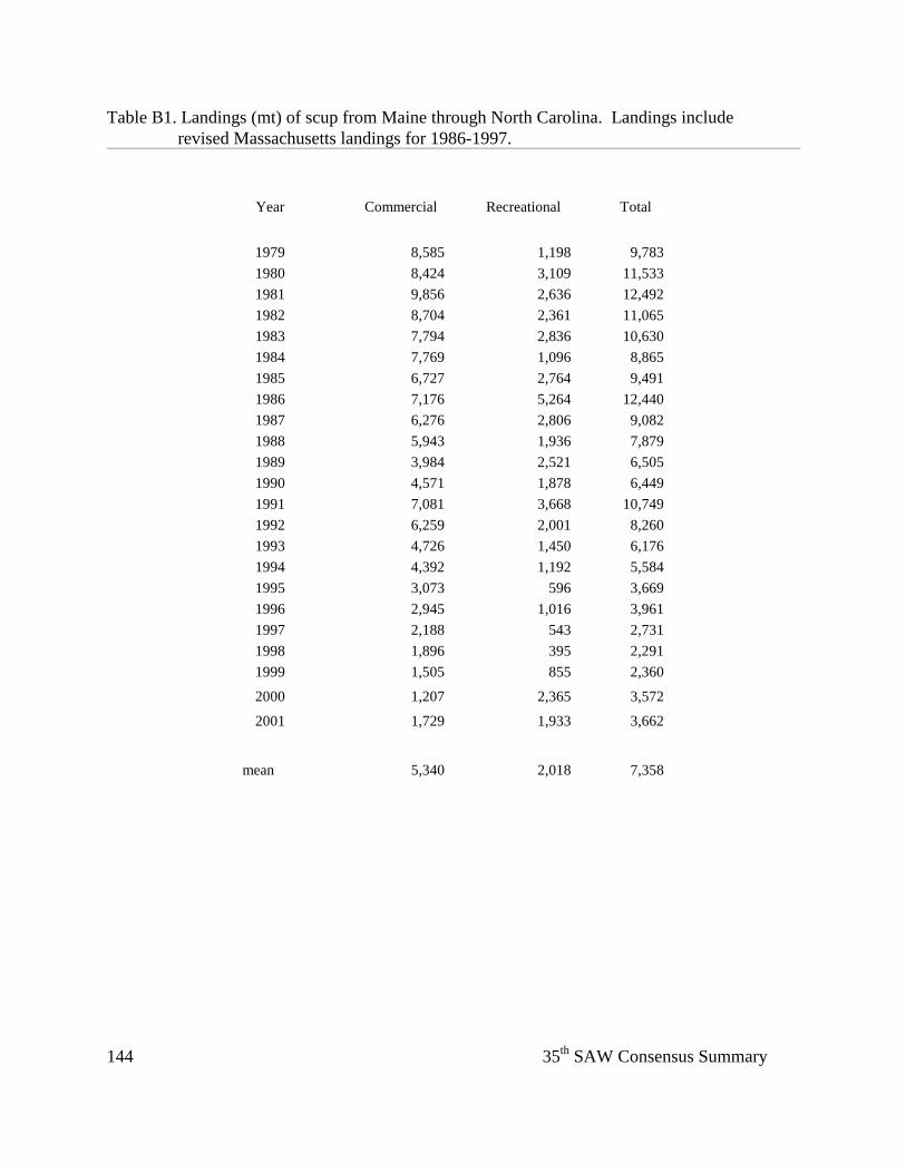
35th SAW Consensus Summary 144
Table B1. Landings (mt) of scup from Maine through North Carolina. Landings include revised Massachusetts landings for 1986-1997.
Year
Commercial
Recreational
Total
1979
8,585
1,198
9,783
1980
8,424
3,109
11,533
1981
9,856
2,636
12,492
1982
8,704
2,361
11,065
1983
7,794
2,836
10,630
1984
7,769
1,096
8,865
1985
6,727
2,764
9,491
1986
7,176
5,264
12,440
1987
6,276
2,806
9,082
1988
5,943
1,936
7,879
1989
3,984
2,521
6,505
1990
4,571
1,878
6,449
1991
7,081
3,668
10,749
1992
6,259
2,001
8,260
1993
4,726
1,450
6,176
1994
4,392
1,192
5,584
1995
3,073
596
3,669
1996
2,945
1,016
3,961
1997
2,188
543
2,731
1998
1,896
395
2,291
1999
1,505
855
2,360
2000
1,207
2,365
3,572
2001
1,729
1,933
3,662
mean
5,340
2,018
7,358
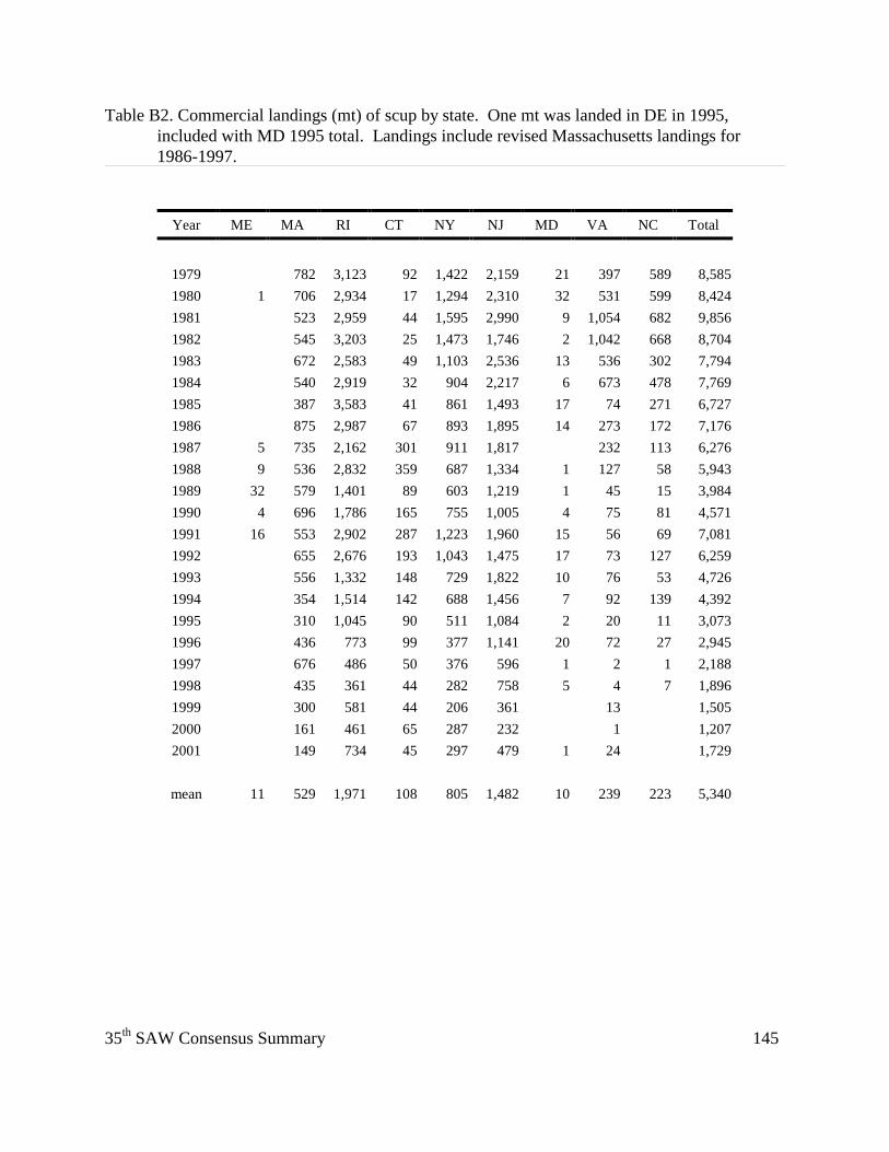
35th SAW Consensus Summary 145
Table B2. Commercial landings (mt) of scup by state. One mt was landed in DE in 1995, included with MD 1995 total. Landings include revised Massachusetts landings for 1986-1997.
Year
ME
MA
RI
CT
NY
NJ
MD
VA
NC
Total
1979
782
3,123
92
1,422
2,159
21
397
589
8,585
1980
1
706
2,934
17
1,294
2,310
32
531
599
8,424 1981
523
2,959
44
1,595
2,990
9
1,054
682
9,856
1982
545
3,203
25
1,473
1,746
2
1,042
668
8,704
1983
672
2,583
49
1,103
2,536
13
536
302
7,794
1984
540
2,919
32
904
2,217
6
673
478
7,769
1985
387
3,583
41
861
1,493
17
74
271
6,727
1986
875
2,987
67
893
1,895
14
273
172
7,176
1987
5
735
2,162
301
911
1,817
232
113
6,276
1988
9
536
2,832
359
687
1,334
1
127
58
5,943 1989
32
579
1,401
89
603
1,219
1
45
15
3,984
1990
4
696
1,786
165
755
1,005
4
75
81
4,571 1991
16
553
2,902
287
1,223
1,960
15
56
69
7,081
1992
655
2,676
193
1,043
1,475
17
73
127
6,259
1993
556
1,332
148
729
1,822
10
76
53
4,726
1994
354
1,514
142
688
1,456
7
92
139
4,392
1995
310
1,045
90
511
1,084
2
20
11
3,073
1996
436
773
99
377
1,141
20
72
27
2,945
1997
676
486
50
376
596
1
2
1
2,188
1998
435
361
44
282
758
5
4
7
1,896
1999
300
581
44
206
361
13
1,505 2000
161
461
65
287
232
1
1,207 2001
149
734
45
297
479
1
24
1,729
mean
11
529
1,971
108
805
1,482
10
239
223
5,340
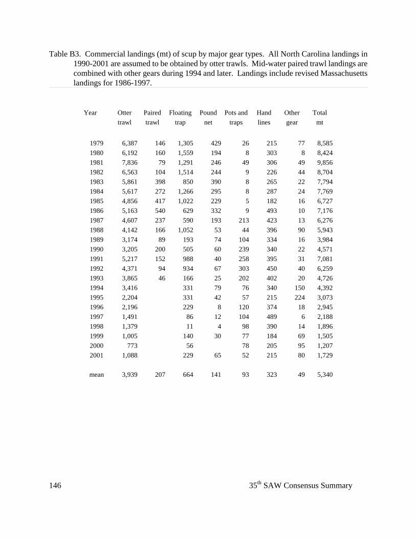
35th SAW Consensus Summary 146
Table B3. Commercial landings (mt) of scup by major gear types. All North Carolina landings in 1990-2001 are assumed to be obtained by otter trawls. Mid-water paired trawl landings are combined with other gears during 1994 and later. Landings include revised Massachusetts landings for 1986-1997.
Year
Otter
Paired
Floating
Pound
Pots and
Hand
Other
Total
trawl
trawl
trap
net
traps
lines
gear
mt
1979
6,387
146
1,305
429
26
215
77
8,585 1980
6,192
160
1,559
194
8
303
8
8,424
1981
7,836
79
1,291
246
49
306
49
9,856 1982
6,563
104
1,514
244
9
226
44
8,704
1983
5,861
398
850
390
8
265
22
7,794 1984
5,617
272
1,266
295
8
287
24
7,769
1985
4,856
417
1,022
229
5
182
16
6,727 1986
5,163
540
629
332
9
493
10
7,176
1987
4,607
237
590
193
213
423
13
6,276 1988
4,142
166
1,052
53
44
396
90
5,943
1989
3,174
89
193
74
104
334
16
3,984 1990
3,205
200
505
60
239
340
22
4,571
1991
5,217
152
988
40
258
395
31
7,081 1992
4,371
94
934
67
303
450
40
6,259
1993
3,865
46
166
25
202
402
20
4,726 1994
3,416
331
79
76
340
150
4,392
1995
2,204
331
42
57
215
224
3,073
1996
2,196
229
8
120
374
18
2,945
1997
1,491
86
12
104
489
6
2,188
1998
1,379
11
4
98
390
14
1,896
1999
1,005
140
30
77
184
69
1,505
2000
773
56
78
205
95
1,207
2001
1,088
229
65
52
215
80
1,729
mean
3,939
207
664
141
93
323
49
5,340
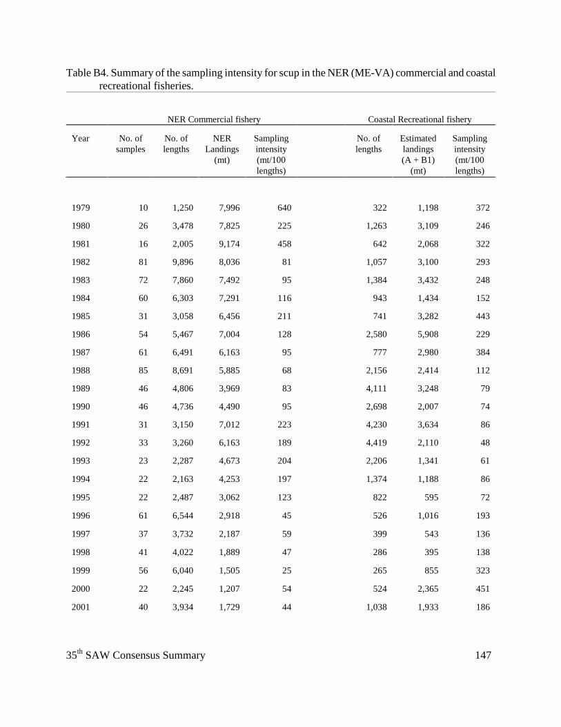
35th SAW Consensus Summary 147
Table B4. Summary of the sampling intensity for scup in the NER (ME-VA) commercial and coastal recreational fisheries.
NER Commercial fishery Coastal Recreational fishery Year
No. of
samples
No. of lengths
NER
Landings (mt)
Sampling intensity (mt/100 lengths)
No. of lengths
Estimated landings (A + B1)
(mt)
Sampling intensity (mt/100 lengths)
1979
10
1,250
7,996
640
322
1,198
372
1980
26
3,478
7,825
225
1,263
3,109
246
1981
16
2,005
9,174
458
642
2,068
322
1982
81
9,896
8,036
81
1,057
3,100
293
1983
72
7,860
7,492
95
1,384
3,432
248
1984
60
6,303
7,291
116
943
1,434
152
1985
31
3,058
6,456
211
741
3,282
443
1986
54
5,467
7,004
128
2,580
5,908
229
1987
61
6,491
6,163
95
777
2,980
384
1988
85
8,691
5,885
68
2,156
2,414
112
1989
46
4,806
3,969
83
4,111
3,248
79
1990
46
4,736
4,490
95
2,698
2,007
74
1991
31
3,150
7,012
223
4,230
3,634
86
1992
33
3,260
6,163
189
4,419
2,110
48
1993
23
2,287
4,673
204
2,206
1,341
61
1994
22
2,163
4,253
197
1,374
1,188
86
1995
22
2,487
3,062
123
822
595
72
1996
61
6,544
2,918
45
526
1,016
193
1997
37
3,732
2,187
59
399
543
136
1998
41
4,022
1,889
47
286
395
138
1999
56
6,040
1,505
25
265
855
323
2000
22
2,245
1,207
54
524
2,365
451
2001
40
3,934
1,729
44
1,038
1,933
186
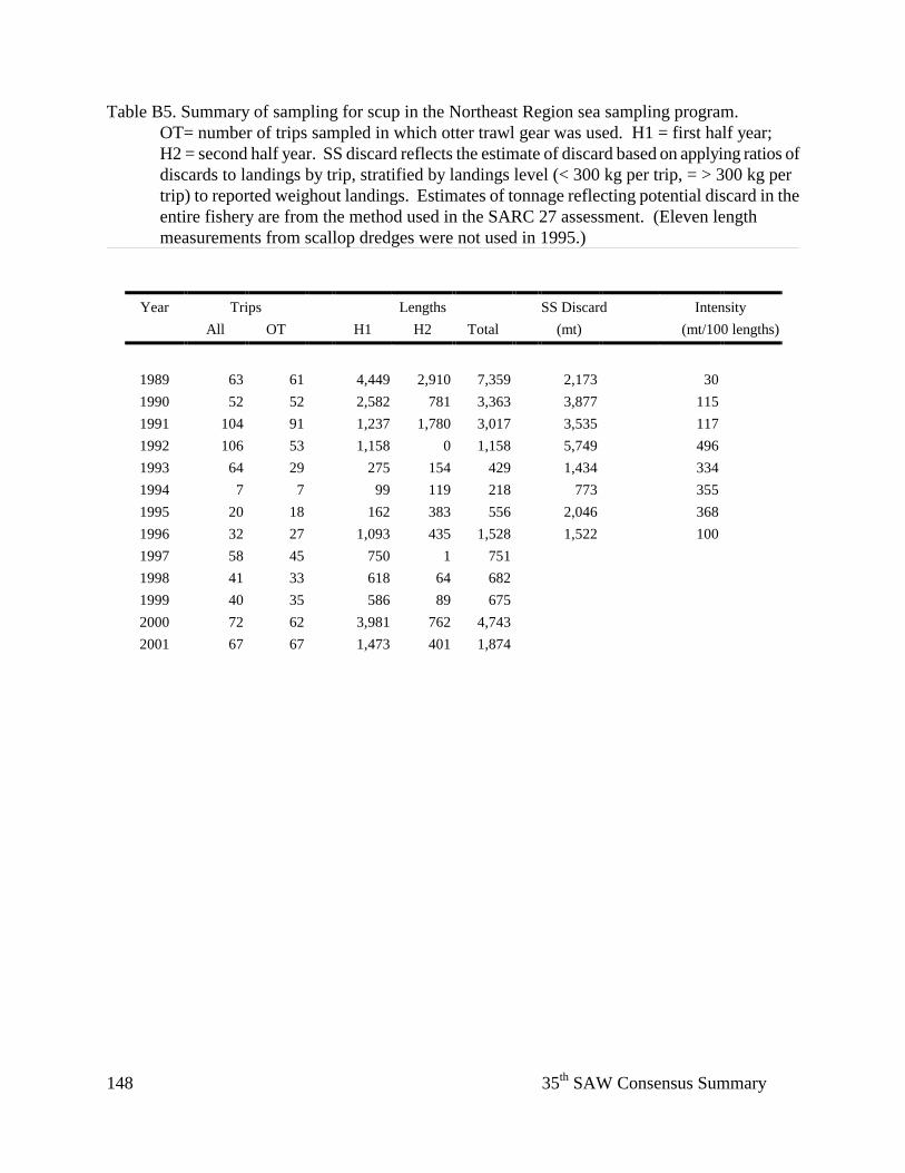
35th SAW Consensus Summary 148
Table B5. Summary of sampling for scup in the Northeast Region sea sampling program.
OT= number of trips sampled in which otter trawl gear was used. H1 = first half year; H2 = second half year. SS discard reflects the estimate of discard based on applying ratios of discards to landings by trip, stratified by landings level (< 300 kg per trip, = > 300 kg per trip) to reported weighout landings. Estimates of tonnage reflecting potential discard in the entire fishery are from the method used in the SARC 27 assessment. (Eleven length measurements from scallop dredges were not used in 1995.)
Year
Trips
Lengths
SS Discard
Intensity
All
OT
H1
H2
Total
(mt)
(mt/100 lengths)
1989
63
61
4,449
2,910
7,359
2,173
30
1990
52
52
2,582
781
3,363
3,877
115
1991
104
91
1,237
1,780
3,017
3,535
117
1992
106
53
1,158
0
1,158
5,749
496
1993
64
29
275
154
429
1,434
334
1994
7
7
99
119
218
773
355
1995
20
18
162
383
556
2,046
368
1996
32
27
1,093
435
1,528
1,522
100
1997
58
45
750
1
751
1998
41
33
618
64
682
1999
40
35
586
89
675
2000
72
62
3,981
762
4,743
2001
67
67
1,473
401
1,874
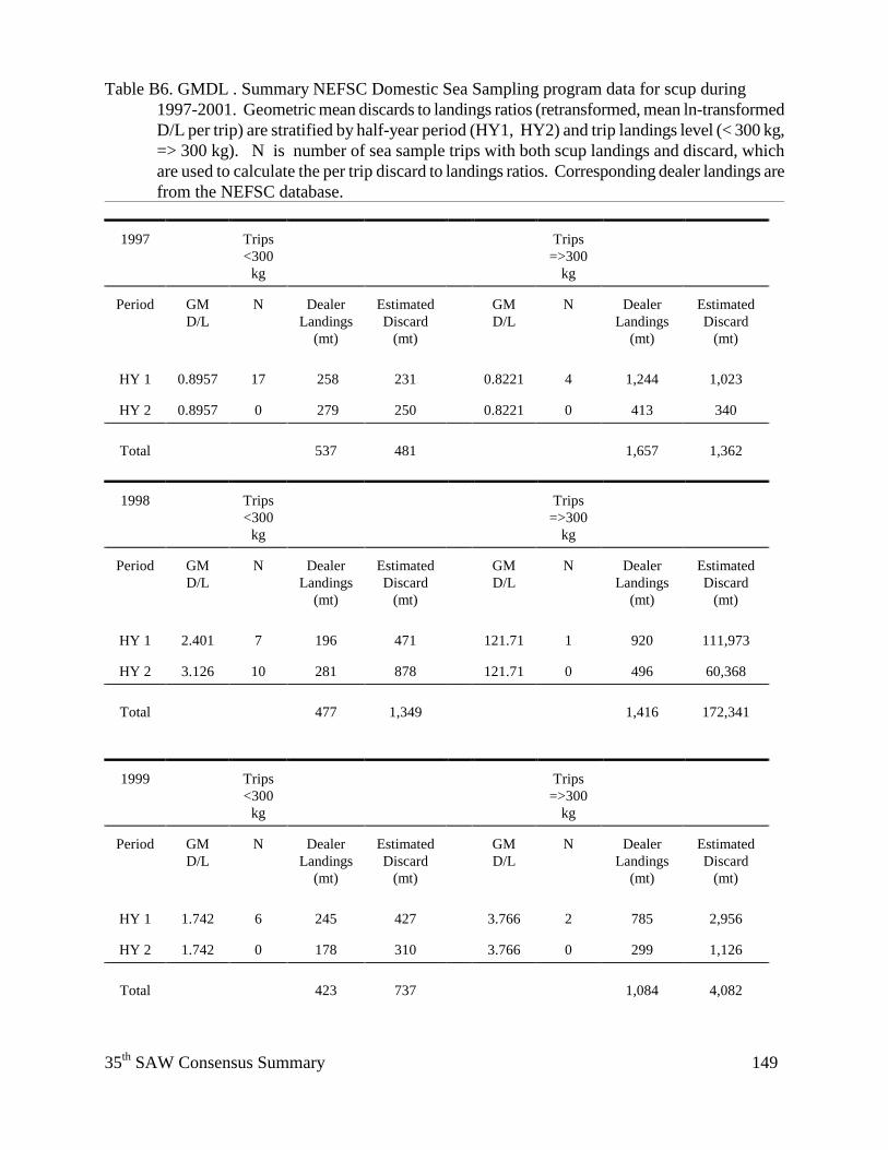
35th SAW Consensus Summary 149
Table B6. GMDL . Summary NEFSC Domestic Sea Sampling program data for scup during 1997-2001. Geometric mean discards to landings ratios (retransformed, mean ln-transformed D/L per trip) are stratified by half-year period (HY1, HY2) and trip landings level (< 300 kg, => 300 kg). N is number of sea sample trips with both scup landings and discard, which are used to calculate the per trip discard to landings ratios. Corresponding dealer landings are from the NEFSC database.
1997
Trips <300
kg
Trips
=>300 kg
Period
GM D/L
N
Dealer
Landings (mt)
Estimated Discard
(mt)
GM D/L
N
Dealer
Landings (mt)
Estimated Discard
(mt) HY 1
0.8957
17
258
231
0.8221
4
1,244
1,023
HY 2
0.8957
0
279
250
0.8221
0
413
340
Total
537
481
1,657
1,362
1998
Trips <300
kg
Trips
=>300 kg
Period
GM D/L
N
Dealer
Landings (mt)
Estimated Discard
(mt)
GM D/L
N
Dealer
Landings (mt)
Estimated Discard
(mt) HY 1
2.401
7
196
471
121.71
1
920
111,973
HY 2
3.126
10
281
878
121.71
0
496
60,368
Total
477
1,349
1,416
172,341
1999
Trips <300
kg
Trips
=>300 kg
Period
GM D/L
N
Dealer
Landings (mt)
Estimated Discard
(mt)
GM D/L
N
Dealer
Landings (mt)
Estimated Discard
(mt) HY 1
1.742
6
245
427
3.766
2
785
2,956
HY 2
1.742
0
178
310
3.766
0
299
1,126
Total
423
737
1,084
4,082
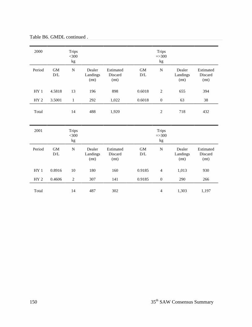
35th SAW Consensus Summary 150
Table B6. GMDL continued .
2000
Trips <300
kg
Trips
=>300 kg
Period
GM D/L
N
Dealer
Landings (mt)
Estimated Discard
(mt)
GM D/L
N
Dealer
Landings (mt)
Estimated Discard
(mt) HY 1
4.5818
13
196
898
0.6018
2
655
394
HY 2
3.5001
1
292
1,022
0.6018
0
63
38
Total
14
488
1,920
2
718
432
2001
Trips <300
kg
Trips
=>300 kg
Period
GM D/L
N
Dealer
Landings (mt)
Estimated Discard
(mt)
GM D/L
N
Dealer
Landings (mt)
Estimated Discard
(mt) HY 1
0.8916
10
180
160
0.9185
4
1,013
930
HY 2
0.4606
2
307
141
0.9185
0
290
266
Total
14
487
302
4
1,303
1,197
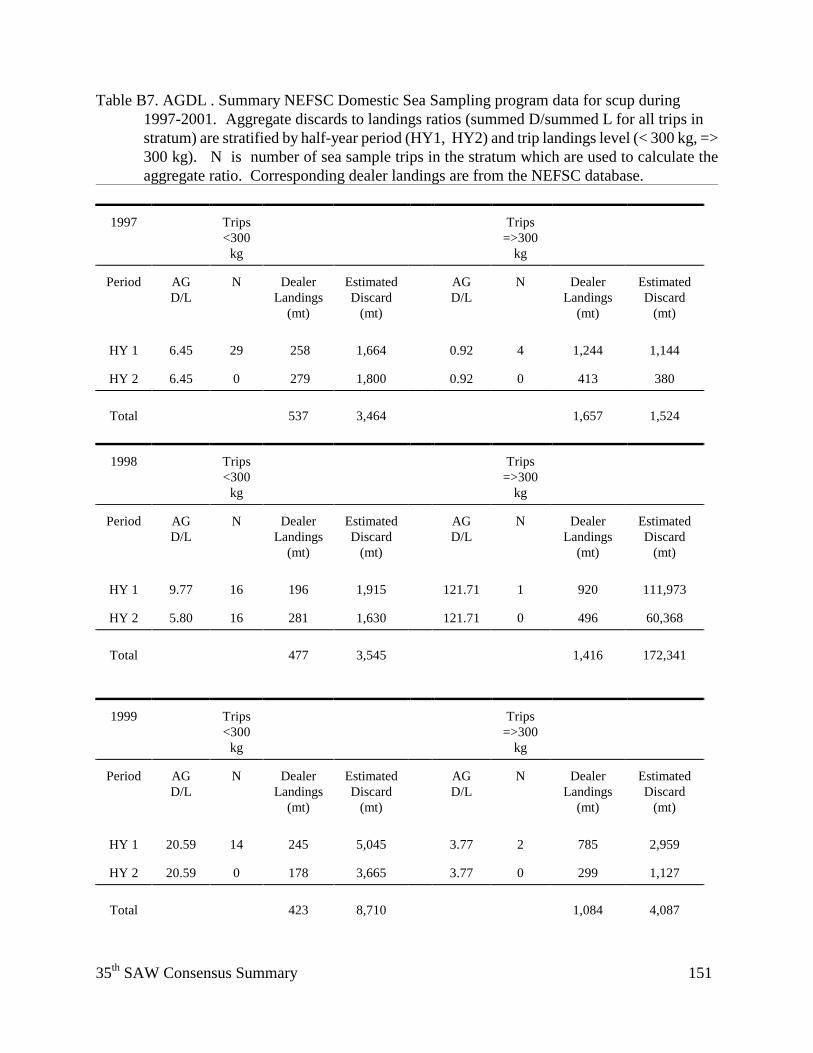
35th SAW Consensus Summary 151
Table B7. AGDL . Summary NEFSC Domestic Sea Sampling program data for scup during
1997-2001. Aggregate discards to landings ratios (summed D/summed L for all trips in stratum) are stratified by half-year period (HY1, HY2) and trip landings level (< 300 kg, => 300 kg). N is number of sea sample trips in the stratum which are used to calculate the aggregate ratio. Corresponding dealer landings are from the NEFSC database.
1997
Trips <300
kg
Trips
=>300 kg
Period
AG D/L
N
Dealer
Landings (mt)
Estimated Discard
(mt)
AG D/L
N
Dealer
Landings (mt)
Estimated Discard
(mt) HY 1
6.45
29
258
1,664
0.92
4
1,244
1,144
HY 2
6.45
0
279
1,800
0.92
0
413
380
Total
537
3,464
1,657
1,524
1998
Trips <300
kg
Trips
=>300 kg
Period
AG D/L
N
Dealer
Landings (mt)
Estimated Discard
(mt)
AG D/L
N
Dealer
Landings (mt)
Estimated Discard
(mt) HY 1
9.77
16
196
1,915
121.71
1
920
111,973
HY 2
5.80
16
281
1,630
121.71
0
496
60,368
Total
477
3,545
1,416
172,341
1999
Trips <300
kg
Trips
=>300 kg
Period
AG D/L
N
Dealer
Landings (mt)
Estimated Discard
(mt)
AG D/L
N
Dealer
Landings (mt)
Estimated Discard
(mt) HY 1
20.59
14
245
5,045
3.77
2
785
2,959
HY 2
20.59
0
178
3,665
3.77
0
299
1,127
Total
423
8,710
1,084
4,087
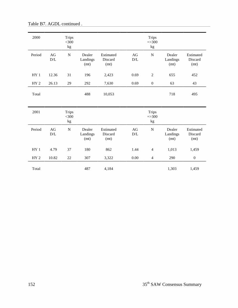
35th SAW Consensus Summary 152
Table B7. AGDL continued .
2000
Trips <300
kg
Trips
=>300 kg
Period
AG D/L
N
Dealer
Landings (mt)
Estimated Discard
(mt)
AG D/L
N
Dealer
Landings (mt)
Estimated Discard
(mt) HY 1
12.36
31
196
2,423
0.69
2
655
452
HY 2
26.13
29
292
7,630
0.69
0
63
43
Total
488
10,053
718
495
2001
Trips <300
kg
Trips
=>300 kg
Period
AG D/L
N
Dealer
Landings (mt)
Estimated Discard
(mt)
AG D/L
N
Dealer
Landings (mt)
Estimated Discard
(mt) HY 1
4.79
37
180
862
1.44
4
1,013
1,459
HY 2
10.82
22
307
3,322
0.00
4
290
0
Total
487
4,184
1,303
1,459
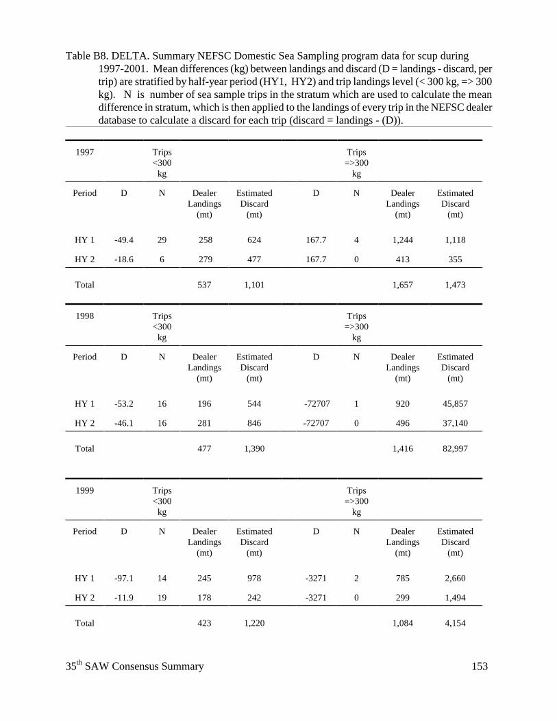
35th SAW Consensus Summary 153
Table B8. DELTA. Summary NEFSC Domestic Sea Sampling program data for scup during 1997-2001. Mean differences (kg) between landings and discard (D = landings - discard, per trip) are stratified by half-year period (HY1, HY2) and trip landings level (< 300 kg, => 300 kg). N is number of sea sample trips in the stratum which are used to calculate the mean difference in stratum, which is then applied to the landings of every trip in the NEFSC dealer database to calculate a discard for each trip (discard = landings - (D)).
1997
Trips <300
kg
Trips
=>300 kg
Period
D
N
Dealer
Landings (mt)
Estimated Discard
(mt)
D
N
Dealer
Landings (mt)
Estimated Discard
(mt) HY 1
-49.4
29
258
624
167.7
4
1,244
1,118
HY 2
-18.6
6
279
477
167.7
0
413
355
Total
537
1,101
1,657
1,473
1998
Trips <300
kg
Trips
=>300 kg
Period
D
N
Dealer
Landings (mt)
Estimated Discard
(mt)
D
N
Dealer
Landings (mt)
Estimated Discard
(mt) HY 1
-53.2
16
196
544
-72707
1
920
45,857
HY 2
-46.1
16
281
846
-72707
0
496
37,140
Total
477
1,390
1,416
82,997
1999
Trips <300
kg
Trips
=>300 kg
Period
D
N
Dealer
Landings (mt)
Estimated Discard
(mt)
D
N
Dealer
Landings (mt)
Estimated Discard
(mt) HY 1
-97.1
14
245
978
-3271
2
785
2,660
HY 2
-11.9
19
178
242
-3271
0
299
1,494
Total
423
1,220
1,084
4,154
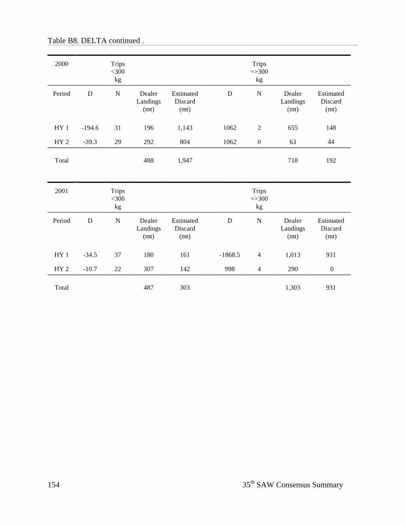
35th SAW Consensus Summary 154
Table B8. DELTA continued .
2000
Trips <300
kg
Trips
=>300 kg
Period
D
N
Dealer
Landings (mt)
Estimated Discard
(mt)
D
N
Dealer
Landings (mt)
Estimated Discard
(mt) HY 1
-194.6
31
196
1,143
1062
2
655
148
HY 2
-39.3
29
292
804
1062
0
63
44
Total
488
1,947
718
192
2001
Trips <300
kg
Trips
=>300 kg
Period
D
N
Dealer
Landings (mt)
Estimated Discard
(mt)
D
N
Dealer
Landings (mt)
Estimated Discard
(mt) HY 1
-34.5
37
180
161
-1868.5
4
1,013
931
HY 2
-10.7
22
307
142
998
4
290
0
Total
487
303
1,303
931
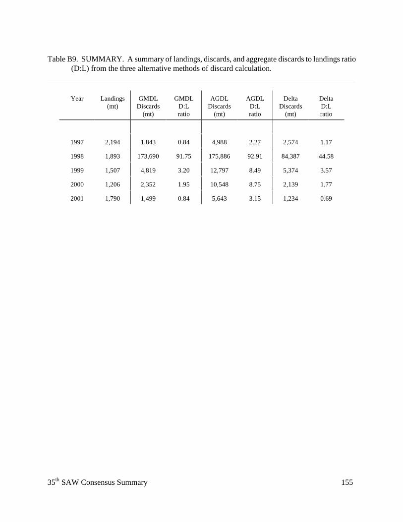
35th SAW Consensus Summary 155
Table B9. SUMMARY. A summary of landings, discards, and aggregate discards to landings ratio
(D:L) from the three alternative methods of discard calculation.
Year Landings
(mt)
GMDL
Discards (mt)
GMDL
D:L ratio
AGDL
Discards (mt)
AGDL
D:L ratio
Delta
Discards (mt)
Delta D:L ratio
1997
2,194
1,843
0.84
4,988
2.27
2,574
1.17
1998
1,893
173,690
91.75
175,886
92.91
84,387
44.58
1999
1,507
4,819
3.20
12,797
8.49
5,374
3.57
2000
1,206
2,352
1.95
10,548
8.75
2,139
1.77
2001
1,790
1,499
0.84
5,643
3.15
1,234
0.69
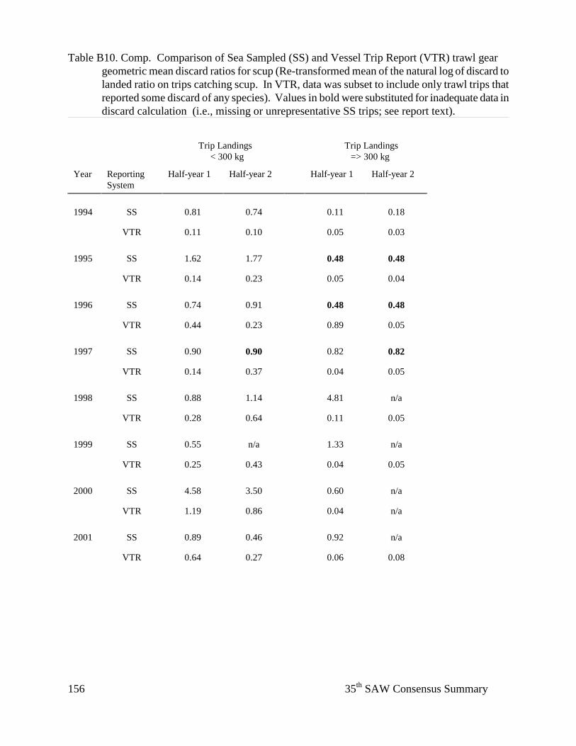
35th SAW Consensus Summary 156
Table B10. Comp. Comparison of Sea Sampled (SS) and Vessel Trip Report (VTR) trawl gear geometric mean discard ratios for scup (Re-transformed mean of the natural log of discard to landed ratio on trips catching scup. In VTR, data was subset to include only trawl trips that reported some discard of any species). Values in bold were substituted for inadequate data in discard calculation (i.e., missing or unrepresentative SS trips; see report text).
Trip Landings Trip Landings < 300 kg => 300 kg
Year
Reporting System
Half-year 1
Half-year 2
Half-year 1
Half-year 2
1994
SS
0.81
0.74
0.11
0.18
VTR
0.11
0.10
0.05
0.03
1995
SS
1.62
1.77
0.48
0.48
VTR
0.14
0.23
0.05
0.04
1996
SS
0.74
0.91
0.48
0.48
VTR
0.44
0.23
0.89
0.05
1997
SS
0.90
0.90
0.82
0.82
VTR
0.14
0.37
0.04
0.05
1998
SS
0.88
1.14
4.81
n/a
VTR
0.28
0.64
0.11
0.05
1999
SS
0.55
n/a
1.33
n/a
VTR
0.25
0.43
0.04
0.05
2000
SS
4.58
3.50
0.60
n/a
VTR
1.19
0.86
0.04
n/a
2001
SS
0.89
0.46
0.92
n/a
VTR
0.64
0.27
0.06
0.08
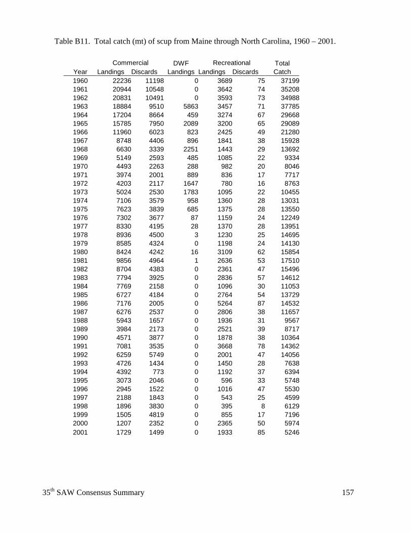
35th SAW Consensus Summary 157
Table B11. Total catch (mt) of scup from Maine through North Carolina, 1960 – 2001.
Commercial DWF Recreational Total Year Landings Discards Landings Landings Discards Catch 1960 22236 11198 0 3689 75 371991961 20944 10548 0 3642 74 352081962 20831 10491 0 3593 73 349881963 18884 9510 5863 3457 71 377851964 17204 8664 459 3274 67 296681965 15785 7950 2089 3200 65 290891966 11960 6023 823 2425 49 212801967 8748 4406 896 1841 38 159281968 6630 3339 2251 1443 29 136921969 5149 2593 485 1085 22 93341970 4493 2263 288 982 20 80461971 3974 2001 889 836 17 77171972 4203 2117 1647 780 16 87631973 5024 2530 1783 1095 22 104551974 7106 3579 958 1360 28 130311975 7623 3839 685 1375 28 135501976 7302 3677 87 1159 24 122491977 8330 4195 28 1370 28 139511978 8936 4500 3 1230 25 146951979 8585 4324 0 1198 24 141301980 8424 4242 16 3109 62 158541981 9856 4964 1 2636 53 175101982 8704 4383 0 2361 47 154961983 7794 3925 0 2836 57 146121984 7769 2158 0 1096 30 110531985 6727 4184 0 2764 54 137291986 7176 2005 0 5264 87 145321987 6276 2537 0 2806 38 116571988 5943 1657 0 1936 31 95671989 3984 2173 0 2521 39 87171990 4571 3877 0 1878 38 103641991 7081 3535 0 3668 78 143621992 6259 5749 0 2001 47 140561993 4726 1434 0 1450 28 76381994 4392 773 0 1192 37 63941995 3073 2046 0 596 33 57481996 2945 1522 0 1016 47 55301997 2188 1843 0 543 25 45991998 1896 3830 0 395 8 61291999 1505 4819 0 855 17 71962000 1207 2352 0 2365 50 59742001 1729 1499 0 1933 85 5246
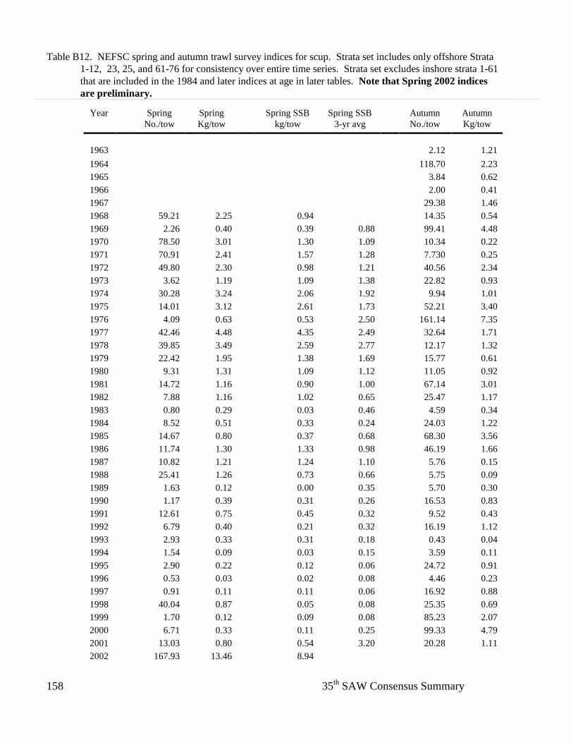
35th SAW Consensus Summary 158
Table B12. NEFSC spring and autumn trawl survey indices for scup. Strata set includes only offshore Strata 1-12, 23, 25, and 61-76 for consistency over entire time series. Strata set excludes inshore strata 1-61 that are included in the 1984 and later indices at age in later tables. Note that Spring 2002 indices are preliminary.
Year
Spring
No./tow
Spring Kg/tow
Spring SSB kg/tow
Spring SSB 3-yr avg
Autumn No./tow
Autumn Kg/tow
1963 2.12 1.21 1964 118.70 2.23 1965 3.84 0.62 1966 2.00 0.41 1967 29.38 1.46 1968 59.21 2.25 0.94 14.35 0.54 1969 2.26 0.40 0.39 0.88 99.41 4.48 1970 78.50 3.01 1.30 1.09 10.34 0.22 1971 70.91 2.41 1.57 1.28 7.730 0.25 1972 49.80 2.30 0.98 1.21 40.56 2.34 1973 3.62 1.19 1.09 1.38 22.82 0.93 1974 30.28 3.24 2.06 1.92 9.94 1.01 1975 14.01 3.12 2.61 1.73 52.21 3.40 1976 4.09 0.63 0.53 2.50 161.14 7.35 1977 42.46 4.48 4.35 2.49 32.64 1.71 1978 39.85 3.49 2.59 2.77 12.17 1.32 1979 22.42 1.95 1.38 1.69 15.77 0.61 1980 9.31 1.31 1.09 1.12 11.05 0.92 1981 14.72 1.16 0.90 1.00 67.14 3.01 1982 7.88 1.16 1.02 0.65 25.47 1.17 1983 0.80 0.29 0.03 0.46 4.59 0.34 1984 8.52 0.51 0.33 0.24 24.03 1.22 1985 14.67 0.80 0.37 0.68 68.30 3.56 1986 11.74 1.30 1.33 0.98 46.19 1.66 1987 10.82 1.21 1.24 1.10 5.76 0.15 1988 25.41 1.26 0.73 0.66 5.75 0.09 1989 1.63 0.12 0.00 0.35 5.70 0.30 1990 1.17 0.39 0.31 0.26 16.53 0.83 1991 12.61 0.75 0.45 0.32 9.52 0.43 1992 6.79 0.40 0.21 0.32 16.19 1.12 1993 2.93 0.33 0.31 0.18 0.43 0.04 1994 1.54 0.09 0.03 0.15 3.59 0.11 1995 2.90 0.22 0.12 0.06 24.72 0.91 1996 0.53 0.03 0.02 0.08 4.46 0.23 1997 0.91 0.11 0.11 0.06 16.92 0.88 1998 40.04 0.87 0.05 0.08 25.35 0.69 1999 1.70 0.12 0.09 0.08 85.23 2.07 2000 6.71 0.33 0.11 0.25 99.33 4.79 2001 13.03 0.80 0.54 3.20 20.28 1.11 2002 167.93 13.46 8.94
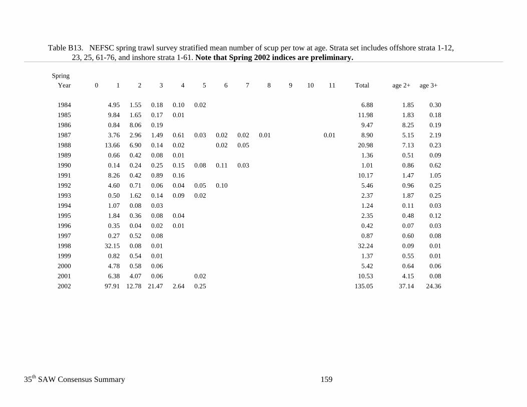
35th SAW Consensus Summary 159
Table B13. NEFSC spring trawl survey stratified mean number of scup per tow at age. Strata set includes offshore strata 1-12, 23, 25, 61-76, and inshore strata 1-61. Note that Spring 2002 indices are preliminary.
Spring
Year
0
1
2
3
4
5
6
7
8
9
10
11
Total
age 2+
age 3+
1984
4.95
1.55
0.18
0.10
0.02
6.88
1.85
0.30 1985
9.84
1.65
0.17
0.01
11.98
1.83
0.18 1986
0.84
8.06
0.19
9.47
8.25
0.19 1987
3.76
2.96
1.49
0.61
0.03
0.02
0.02
0.01
0.01
8.90
5.15
2.19 1988
13.66
6.90
0.14
0.02
0.02
0.05
20.98
7.13
0.23 1989
0.66
0.42
0.08
0.01
1.36
0.51
0.09 1990
0.14
0.24
0.25
0.15
0.08
0.11
0.03
1.01
0.86
0.62 1991
8.26
0.42
0.89
0.16
10.17
1.47
1.05 1992
4.60
0.71
0.06
0.04
0.05
0.10
5.46
0.96
0.25 1993
0.50
1.62
0.14
0.09
0.02
2.37
1.87
0.25 1994
1.07
0.08
0.03
1.24
0.11
0.03 1995
1.84
0.36
0.08
0.04
2.35
0.48
0.12 1996
0.35
0.04
0.02
0.01
0.42
0.07
0.03 1997
0.27
0.52
0.08
0.87
0.60
0.08 1998
32.15
0.08
0.01
32.24
0.09
0.01 1999
0.82
0.54
0.01
1.37
0.55
0.01 2000
4.78
0.58
0.06
5.42
0.64
0.06 2001
6.38
4.07
0.06
0.02
10.53
4.15
0.08 2002
97.91
12.78
21.47
2.64
0.25
135.05
37.14
24.36
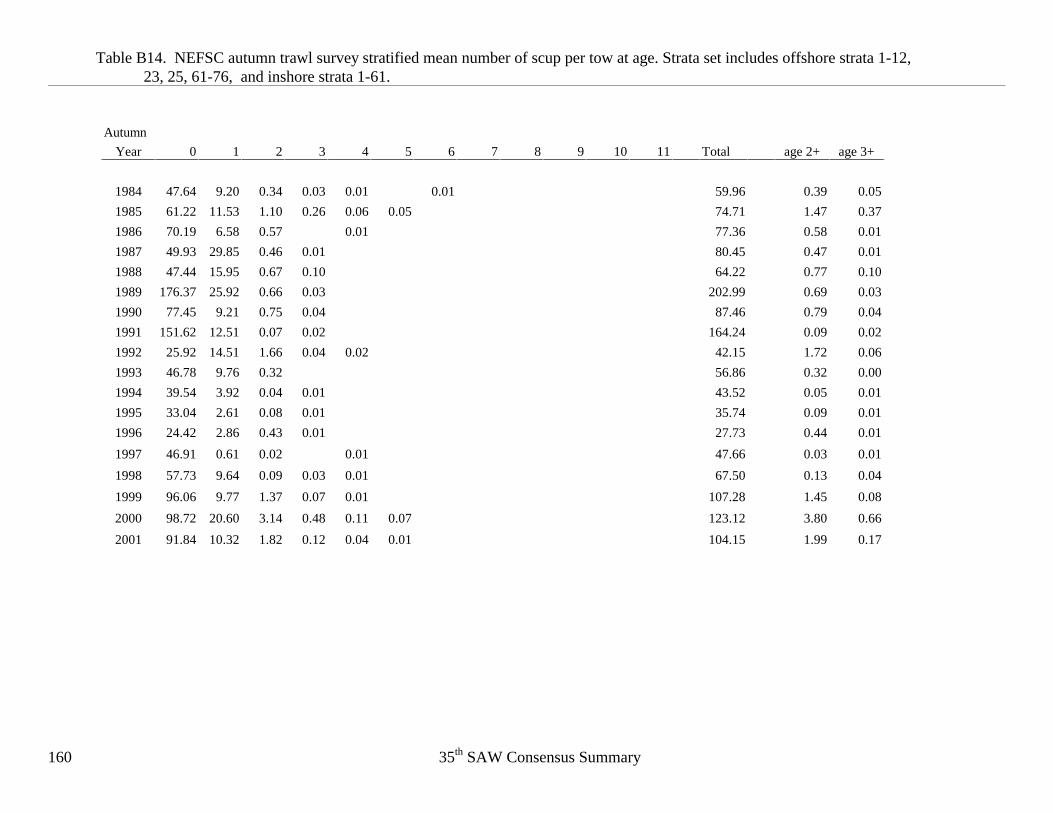
35th SAW Consensus Summary 160
Table B14. NEFSC autumn trawl survey stratified mean number of scup per tow at age. Strata set includes offshore strata 1-12, 23, 25, 61-76, and inshore strata 1-61.
Autumn
Year
0
1
2
3
4
5
6
7
8
9
10
11
Total
age 2+
age 3+
1984
47.64
9.20
0.34
0.03
0.01
0.01
59.96
0.39
0.05 1985
61.22
11.53
1.10
0.26
0.06
0.05
74.71
1.47
0.37 1986
70.19
6.58
0.57
0.01
77.36
0.58
0.01 1987
49.93
29.85
0.46
0.01
80.45
0.47
0.01 1988
47.44
15.95
0.67
0.10
64.22
0.77
0.10 1989
176.37
25.92
0.66
0.03
202.99
0.69
0.03 1990
77.45
9.21
0.75
0.04
87.46
0.79
0.04 1991
151.62
12.51
0.07
0.02
164.24
0.09
0.02 1992
25.92
14.51
1.66
0.04
0.02
42.15
1.72
0.06 1993
46.78
9.76
0.32
56.86
0.32
0.00 1994
39.54
3.92
0.04
0.01
43.52
0.05
0.01 1995
33.04
2.61
0.08
0.01
35.74
0.09
0.01 1996
24.42
2.86
0.43
0.01
27.73
0.44
0.01
1997
46.91
0.61
0.02
0.01
47.66
0.03
0.01
1998
57.73
9.64
0.09
0.03
0.01
67.50
0.13
0.04
1999
96.06
9.77
1.37
0.07
0.01
107.28
1.45
0.08
2000
98.72
20.60
3.14
0.48
0.11
0.07
123.12
3.80
0.66
2001
91.84
10.32
1.82
0.12
0.04
0.01
104.15
1.99
0.17
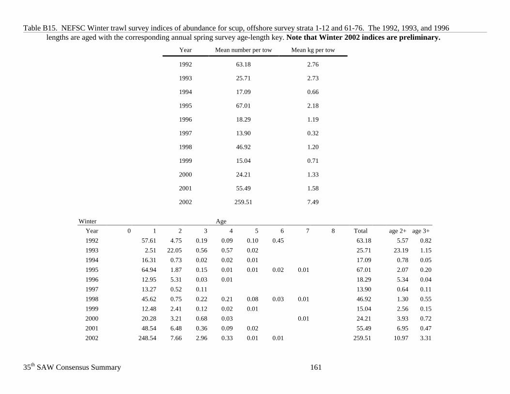
35th SAW Consensus Summary 161
Table B15. NEFSC Winter trawl survey indices of abundance for scup, offshore survey strata 1-12 and 61-76. The 1992, 1993, and 1996 lengths are aged with the corresponding annual spring survey age-length key. Note that Winter 2002 indices are preliminary.
Year
Mean number per tow
Mean kg per tow
1992
63.18
2.76
1993
25.71
2.73
1994
17.09
0.66
1995
67.01
2.18
1996
18.29
1.19
1997
13.90
0.32
1998
46.92
1.20
1999
15.04
0.71
2000
24.21
1.33
2001
55.49
1.58
2002
259.51
7.49
Winter
Age
Year
0
1
2
3
4
5
6
7
8
Total
age 2+
age 3+
1992
57.61
4.75
0.19
0.09
0.10
0.45
63.18
5.57
0.82 1993
2.51
22.05
0.56
0.57
0.02
25.71
23.19
1.15 1994
16.31
0.73
0.02
0.02
0.01
17.09
0.78
0.05 1995
64.94
1.87
0.15
0.01
0.01
0.02
0.01
67.01
2.07
0.20 1996
12.95
5.31
0.03
0.01
18.29
5.34
0.04 1997
13.27
0.52
0.11
13.90
0.64
0.11 1998
45.62
0.75
0.22
0.21
0.08
0.03
0.01
46.92
1.30
0.55 1999
12.48
2.41
0.12
0.02
0.01
15.04
2.56
0.15 2000
20.28
3.21
0.68
0.03
0.01
24.21
3.93
0.72 2001
48.54
6.48
0.36
0.09
0.02
55.49
6.95
0.47 2002
248.54
7.66
2.96
0.33
0.01
0.01
259.51
10.97
3.31
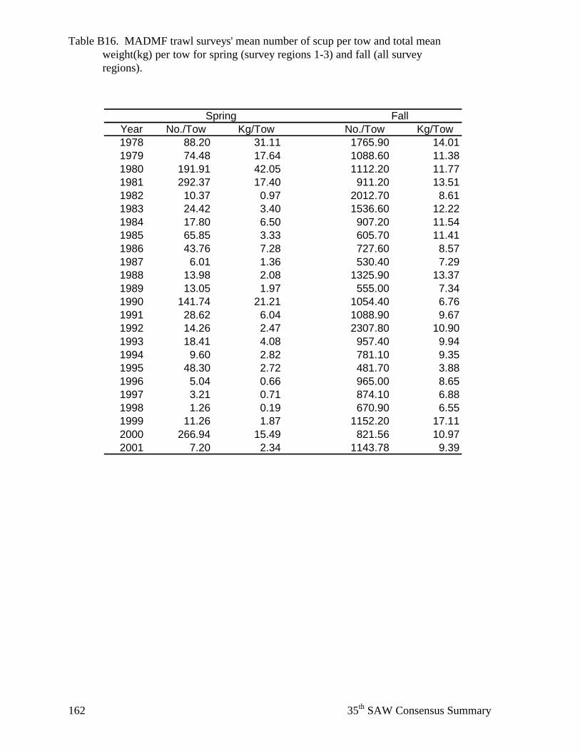
35th SAW Consensus Summary 162
Table B16. MADMF trawl surveys' mean number of scup per tow and total mean weight(kg) per tow for spring (survey regions 1-3) and fall (all survey regions).
Spring FallYear No./Tow Kg/Tow No./Tow Kg/Tow1978 88.20 31.11 1765.90 14.011979 74.48 17.64 1088.60 11.381980 191.91 42.05 1112.20 11.771981 292.37 17.40 911.20 13.511982 10.37 0.97 2012.70 8.611983 24.42 3.40 1536.60 12.221984 17.80 6.50 907.20 11.541985 65.85 3.33 605.70 11.411986 43.76 7.28 727.60 8.571987 6.01 1.36 530.40 7.291988 13.98 2.08 1325.90 13.371989 13.05 1.97 555.00 7.341990 141.74 21.21 1054.40 6.761991 28.62 6.04 1088.90 9.671992 14.26 2.47 2307.80 10.901993 18.41 4.08 957.40 9.941994 9.60 2.82 781.10 9.351995 48.30 2.72 481.70 3.881996 5.04 0.66 965.00 8.651997 3.21 0.71 874.10 6.881998 1.26 0.19 670.90 6.551999 11.26 1.87 1152.20 17.112000 266.94 15.49 821.56 10.972001 7.20 2.34 1143.78 9.39
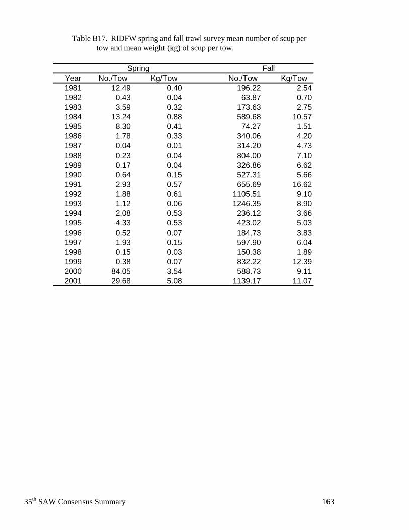
35th SAW Consensus Summary 163
Table B17. RIDFW spring and fall trawl survey mean number of scup per
tow and mean weight (kg) of scup per tow.
Spring FallYear No./Tow Kg/Tow No./Tow Kg/Tow1981 12.49 0.40 196.22 2.541982 0.43 0.04 63.87 0.701983 3.59 0.32 173.63 2.751984 13.24 0.88 589.68 10.571985 8.30 0.41 74.27 1.511986 1.78 0.33 340.06 4.201987 0.04 0.01 314.20 4.731988 0.23 0.04 804.00 7.101989 0.17 0.04 326.86 6.621990 0.64 0.15 527.31 5.661991 2.93 0.57 655.69 16.621992 1.88 0.61 1105.51 9.101993 1.12 0.06 1246.35 8.901994 2.08 0.53 236.12 3.661995 4.33 0.53 423.02 5.031996 0.52 0.07 184.73 3.831997 1.93 0.15 597.90 6.041998 0.15 0.03 150.38 1.891999 0.38 0.07 832.22 12.392000 84.05 3.54 588.73 9.112001 29.68 5.08 1139.17 11.07
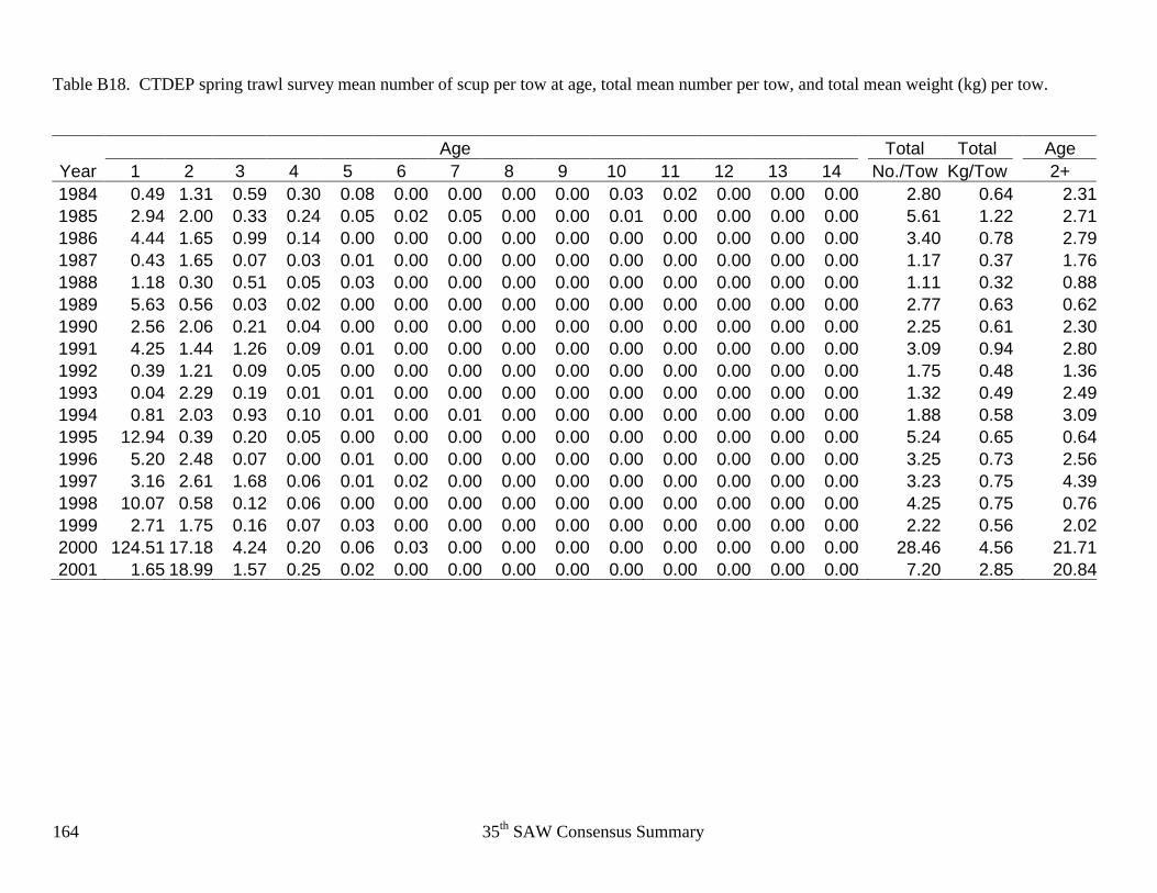
35th SAW Consensus Summary 164
Table B18. CTDEP spring trawl survey mean number of scup per tow at age, total mean number per tow, and total mean weight (kg) per tow. Age Total Total Age Year 1 2 3 4 5 6 7 8 9 10 11 12 13 14 No./Tow Kg/Tow 2+ 1984 0.49 1.31 0.59 0.30 0.08 0.00 0.00 0.00 0.00 0.03 0.02 0.00 0.00 0.00 2.80 0.64 2.311985 2.94 2.00 0.33 0.24 0.05 0.02 0.05 0.00 0.00 0.01 0.00 0.00 0.00 0.00 5.61 1.22 2.711986 4.44 1.65 0.99 0.14 0.00 0.00 0.00 0.00 0.00 0.00 0.00 0.00 0.00 0.00 3.40 0.78 2.791987 0.43 1.65 0.07 0.03 0.01 0.00 0.00 0.00 0.00 0.00 0.00 0.00 0.00 0.00 1.17 0.37 1.761988 1.18 0.30 0.51 0.05 0.03 0.00 0.00 0.00 0.00 0.00 0.00 0.00 0.00 0.00 1.11 0.32 0.881989 5.63 0.56 0.03 0.02 0.00 0.00 0.00 0.00 0.00 0.00 0.00 0.00 0.00 0.00 2.77 0.63 0.621990 2.56 2.06 0.21 0.04 0.00 0.00 0.00 0.00 0.00 0.00 0.00 0.00 0.00 0.00 2.25 0.61 2.301991 4.25 1.44 1.26 0.09 0.01 0.00 0.00 0.00 0.00 0.00 0.00 0.00 0.00 0.00 3.09 0.94 2.801992 0.39 1.21 0.09 0.05 0.00 0.00 0.00 0.00 0.00 0.00 0.00 0.00 0.00 0.00 1.75 0.48 1.361993 0.04 2.29 0.19 0.01 0.01 0.00 0.00 0.00 0.00 0.00 0.00 0.00 0.00 0.00 1.32 0.49 2.491994 0.81 2.03 0.93 0.10 0.01 0.00 0.01 0.00 0.00 0.00 0.00 0.00 0.00 0.00 1.88 0.58 3.091995 12.94 0.39 0.20 0.05 0.00 0.00 0.00 0.00 0.00 0.00 0.00 0.00 0.00 0.00 5.24 0.65 0.641996 5.20 2.48 0.07 0.00 0.01 0.00 0.00 0.00 0.00 0.00 0.00 0.00 0.00 0.00 3.25 0.73 2.561997 3.16 2.61 1.68 0.06 0.01 0.02 0.00 0.00 0.00 0.00 0.00 0.00 0.00 0.00 3.23 0.75 4.391998 10.07 0.58 0.12 0.06 0.00 0.00 0.00 0.00 0.00 0.00 0.00 0.00 0.00 0.00 4.25 0.75 0.761999 2.71 1.75 0.16 0.07 0.03 0.00 0.00 0.00 0.00 0.00 0.00 0.00 0.00 0.00 2.22 0.56 2.022000 124.51 17.18 4.24 0.20 0.06 0.03 0.00 0.00 0.00 0.00 0.00 0.00 0.00 0.00 28.46 4.56 21.712001 1.65 18.99 1.57 0.25 0.02 0.00 0.00 0.00 0.00 0.00 0.00 0.00 0.00 0.00 7.20 2.85 20.84
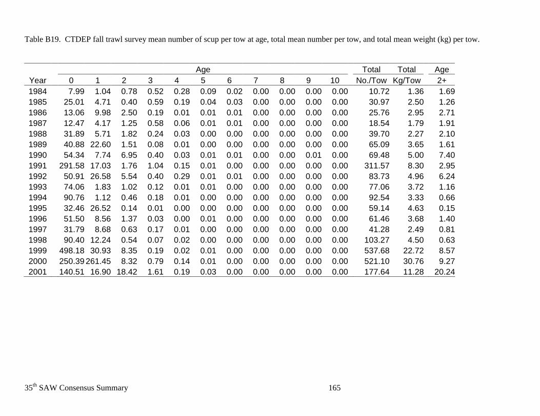
35th SAW Consensus Summary 165
Table B19. CTDEP fall trawl survey mean number of scup per tow at age, total mean number per tow, and total mean weight (kg) per tow. Age Total Total Age
Year 0 1 2 3 4 5 6 7 8 9 10 No./Tow Kg/Tow 2+ 1984 7.99 1.04 0.78 0.52 0.28 0.09 0.02 0.00 0.00 0.00 0.00 10.72 1.36 1.691985 25.01 4.71 0.40 0.59 0.19 0.04 0.03 0.00 0.00 0.00 0.00 30.97 2.50 1.261986 13.06 9.98 2.50 0.19 0.01 0.01 0.01 0.00 0.00 0.00 0.00 25.76 2.95 2.711987 12.47 4.17 1.25 0.58 0.06 0.01 0.01 0.00 0.00 0.00 0.00 18.54 1.79 1.911988 31.89 5.71 1.82 0.24 0.03 0.00 0.00 0.00 0.00 0.00 0.00 39.70 2.27 2.101989 40.88 22.60 1.51 0.08 0.01 0.00 0.00 0.00 0.00 0.00 0.00 65.09 3.65 1.611990 54.34 7.74 6.95 0.40 0.03 0.01 0.01 0.00 0.00 0.01 0.00 69.48 5.00 7.401991 291.58 17.03 1.76 1.04 0.15 0.01 0.00 0.00 0.00 0.00 0.00 311.57 8.30 2.951992 50.91 26.58 5.54 0.40 0.29 0.01 0.01 0.00 0.00 0.00 0.00 83.73 4.96 6.241993 74.06 1.83 1.02 0.12 0.01 0.01 0.00 0.00 0.00 0.00 0.00 77.06 3.72 1.161994 90.76 1.12 0.46 0.18 0.01 0.00 0.00 0.00 0.00 0.00 0.00 92.54 3.33 0.661995 32.46 26.52 0.14 0.01 0.00 0.00 0.00 0.00 0.00 0.00 0.00 59.14 4.63 0.151996 51.50 8.56 1.37 0.03 0.00 0.01 0.00 0.00 0.00 0.00 0.00 61.46 3.68 1.401997 31.79 8.68 0.63 0.17 0.01 0.00 0.00 0.00 0.00 0.00 0.00 41.28 2.49 0.811998 90.40 12.24 0.54 0.07 0.02 0.00 0.00 0.00 0.00 0.00 0.00 103.27 4.50 0.631999 498.18 30.93 8.35 0.19 0.02 0.01 0.00 0.00 0.00 0.00 0.00 537.68 22.72 8.572000 250.39 261.45 8.32 0.79 0.14 0.01 0.00 0.00 0.00 0.00 0.00 521.10 30.76 9.272001 140.51 16.90 18.42 1.61 0.19 0.03 0.00 0.00 0.00 0.00 0.00 177.64 11.28 20.24
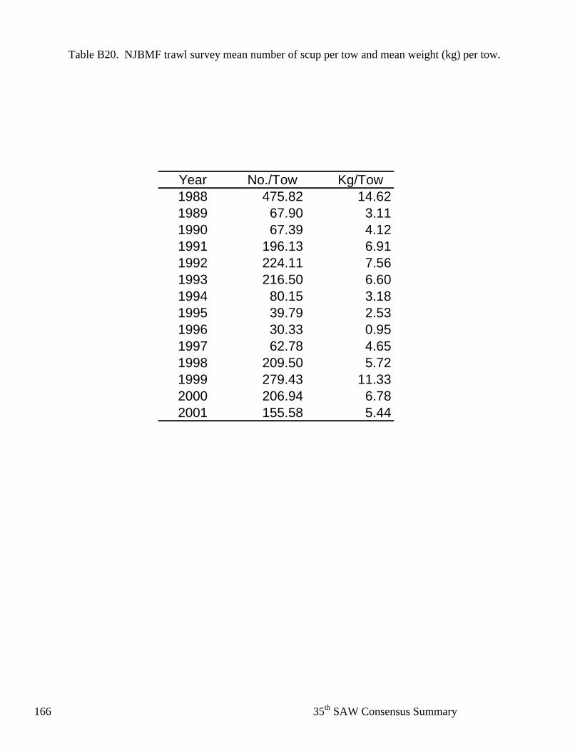
35th SAW Consensus Summary 166
Table B20. NJBMF trawl survey mean number of scup per tow and mean weight (kg) per tow.
Year No./Tow Kg/Tow1988 475.82 14.621989 67.90 3.111990 67.39 4.121991 196.13 6.911992 224.11 7.561993 216.50 6.601994 80.15 3.181995 39.79 2.531996 30.33 0.951997 62.78 4.651998 209.50 5.721999 279.43 11.332000 206.94 6.782001 155.58 5.44
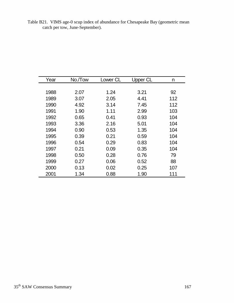
35th SAW Consensus Summary 167
Table B21. VIMS age-0 scup index of abundance for Chesapeake Bay (geometric mean
catch per tow, June-September).
Year No./Tow Lower CL Upper CL n
1988 2.07 1.24 3.21 921989 3.07 2.05 4.41 1121990 4.92 3.14 7.45 1121991 1.90 1.11 2.99 1031992 0.65 0.41 0.93 1041993 3.36 2.16 5.01 1041994 0.90 0.53 1.35 1041995 0.39 0.21 0.59 1041996 0.54 0.29 0.83 1041997 0.21 0.09 0.35 1041998 0.50 0.28 0.76 791999 0.27 0.06 0.52 882000 0.13 0.02 0.25 1072001 1.34 0.88 1.90 111
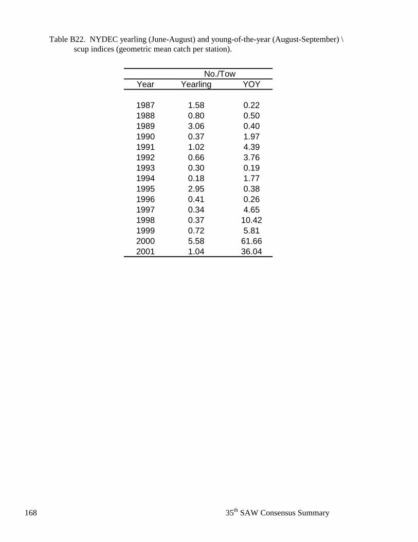
35th SAW Consensus Summary 168
Table B22. NYDEC yearling (June-August) and young-of-the-year (August-September) \
scup indices (geometric mean catch per station).
No./TowYear Yearling YOY
1987 1.58 0.221988 0.80 0.501989 3.06 0.401990 0.37 1.971991 1.02 4.391992 0.66 3.761993 0.30 0.191994 0.18 1.771995 2.95 0.381996 0.41 0.261997 0.34 4.651998 0.37 10.421999 0.72 5.812000 5.58 61.662001 1.04 36.04
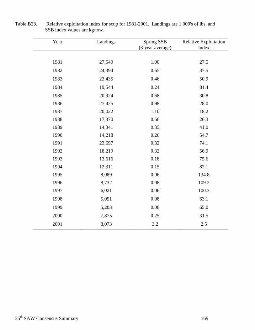
35th SAW Consensus Summary 169
Table B23. Relative exploitation index for scup for 1981-2001. Landings are 1,000's of lbs. and SSB index values are kg/tow.
Year Landings Spring SSB
(3-year average) Relative Exploitation
Index
1981 27,540 1.00 27.5
1982 24,394 0.65 37.5
1983 23,435 0.46 50.9
1984 19,544 0.24 81.4
1985 20,924 0.68 30.8
1986 27,425 0.98 28.0
1987 20,022 1.10 18.2
1988 17,370 0.66 26.3
1989 14,341 0.35 41.0
1990 14,218 0.26 54.7
1991 23,697 0.32 74.1
1992 18,210 0.32 56.9
1993 13,616 0.18 75.6
1994 12,311 0.15 82.1
1995 8,089 0.06 134.8
1996 8,732 0.08 109.2
1997 6,021 0.06 100.3
1998 5,051 0.08 63.1
1999 5,203 0.08 65.0
2000 7,875 0.25 31.5
2001 8,073 3.2 2.5
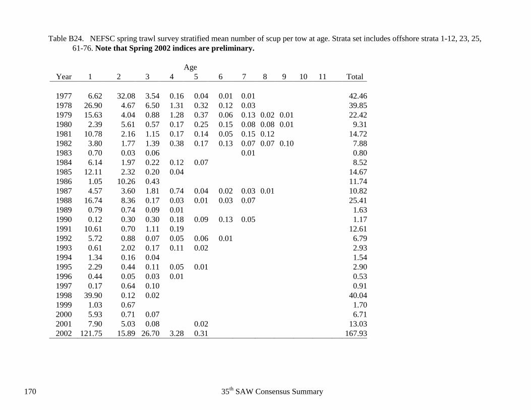
35th SAW Consensus Summary 170
Table B24. NEFSC spring trawl survey stratified mean number of scup per tow at age. Strata set includes offshore strata 1-12, 23, 25, 61-76. Note that Spring 2002 indices are preliminary.
Age
Year 1 2 3 4 5 6 7 8 9 10 11 Total
1977 6.62 32.08 3.54 0.16 0.04 0.01 0.01 42.461978 26.90 4.67 6.50 1.31 0.32 0.12 0.03 39.851979 15.63 4.04 0.88 1.28 0.37 0.06 0.13 0.02 0.01 22.421980 2.39 5.61 0.57 0.17 0.25 0.15 0.08 0.08 0.01 9.311981 10.78 2.16 1.15 0.17 0.14 0.05 0.15 0.12 14.721982 3.80 1.77 1.39 0.38 0.17 0.13 0.07 0.07 0.10 7.881983 0.70 0.03 0.06 0.01 0.801984 6.14 1.97 0.22 0.12 0.07 8.521985 12.11 2.32 0.20 0.04 14.671986 1.05 10.26 0.43 11.741987 4.57 3.60 1.81 0.74 0.04 0.02 0.03 0.01 10.821988 16.74 8.36 0.17 0.03 0.01 0.03 0.07 25.411989 0.79 0.74 0.09 0.01 1.631990 0.12 0.30 0.30 0.18 0.09 0.13 0.05 1.171991 10.61 0.70 1.11 0.19 12.611992 5.72 0.88 0.07 0.05 0.06 0.01 6.791993 0.61 2.02 0.17 0.11 0.02 2.931994 1.34 0.16 0.04 1.541995 2.29 0.44 0.11 0.05 0.01 2.901996 0.44 0.05 0.03 0.01 0.531997 0.17 0.64 0.10 0.911998 39.90 0.12 0.02 40.041999 1.03 0.67 1.702000 5.93 0.71 0.07 6.712001 7.90 5.03 0.08 0.02 13.032002 121.75 15.89 26.70 3.28 0.31 167.93
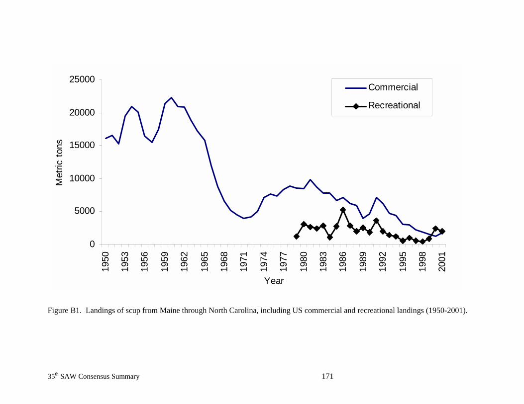
35th SAW Consensus Summary 171
Figure B1. Landings of scup from Maine through North Carolina, including US commercial and recreational landings (1950-2001).
0
5000
10000
15000
20000
25000
1950
1953
1956
1959
1962
1965
1968
1971
1974
1977
1980
1983
1986
1989
1992
1995
1998
2001
Year
Met
ric to
ns
Commercial
Recreational
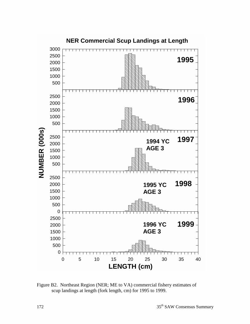
172 35th SAW Consensus Summary
Figure B2. Northeast Region (NER; ME to VA) commercial fishery estimates of
scup landings at length (fork length, cm) for 1995 to 1999.
NER Commercial Scup Landings at Length
1995
50010001500200025003000
5001000150020002500
NU
MB
ER (0
00s)
5001000150020002500 1996
19971994 YCAGE 3
0500
1000150020002500
1998
LENGTH (cm)0 5 10 15 20 25 30 35 40
0500
1000150020002500
1999
1995 YCAGE 3
1996 YCAGE 3
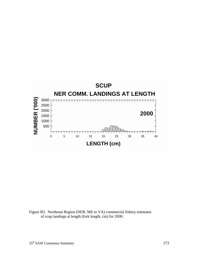
35th SAW Consensus Summary 173
Figure B3. Northeast Region (NER; ME to VA) commercial fishery estimates
of scup landings at length (fork length, cm) for 2000.
NER COMM. LANDINGS AT LENGTHSCUP
2000
LENGTH (cm)0 5 10 15 20 25 30 35 40
NU
MB
ER ('
000)
50010001500200025003000
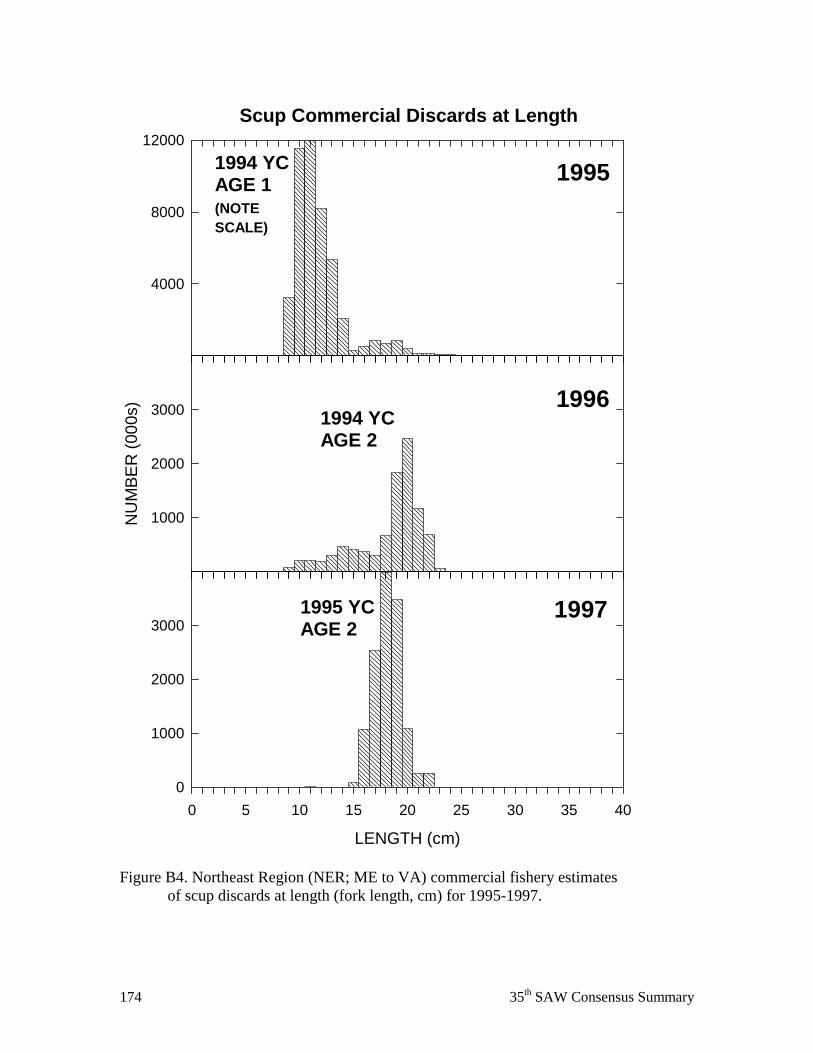
174 35th SAW Consensus Summary
Figure B4. Northeast Region (NER; ME to VA) commercial fishery estimates
of scup discards at length (fork length, cm) for 1995-1997.
Scup Commercial Discards at Length
1995
4000
8000
12000
LENGTH (cm)
0 5 10 15 20 25 30 35 400
1000
2000
3000
NU
MBE
R (0
00s)
1000
2000
3000 1996
1997
1994 YCAGE 1(NOTESCALE)
1994 YCAGE 2
1995 YCAGE 2
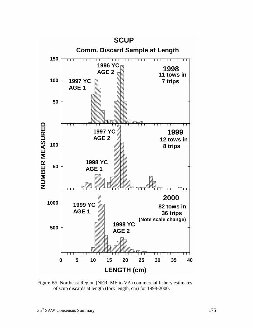
35th SAW Consensus Summary 175
Figure B5. Northeast Region (NER; ME to VA) commercial fishery estimates
of scup discards at length (fork length, cm) for 1998-2000.
Comm. Discard Sample at LengthSCUP
1998
50
100
150
1997 YCAGE 1
1996 YCAGE 2
NU
MB
ER M
EASU
RED
50
100
19991997 YCAGE 2
1998 YCAGE 1
11 tows in 7 trips
12 tows in 8 trips
LENGTH (cm)0 5 10 15 20 25 30 35 40
500
10002000
82 tows in 36 trips
1999 YCAGE 1
1998 YCAGE 2
(Note scale change)
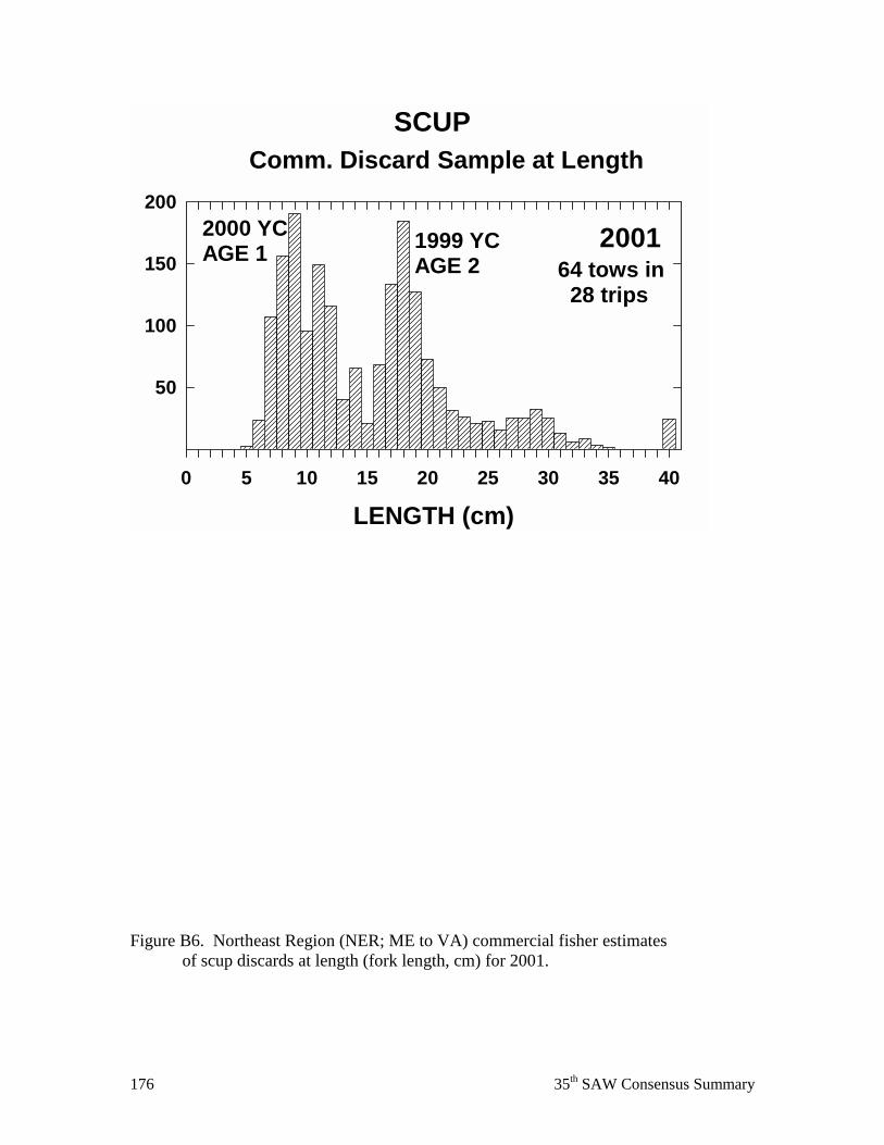
176 35th SAW Consensus Summary
Figure B6. Northeast Region (NER; ME to VA) commercial fisher estimates
of scup discards at length (fork length, cm) for 2001.
Comm. Discard Sample at LengthSCUP
LENGTH (cm)0 5 10 15 20 25 30 35 40
50
100
150
200
200164 tows in 28 trips
1999 YCAGE 2
2000 YCAGE 1
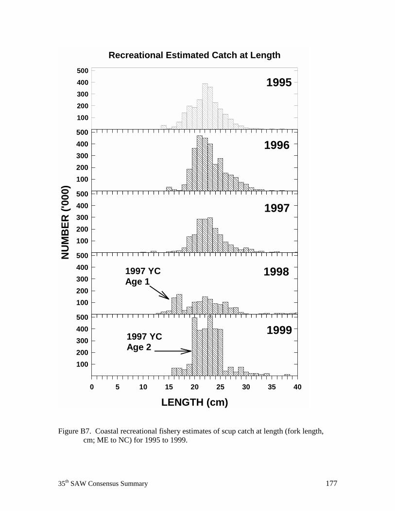
35th SAW Consensus Summary 177
Figure B7. Coastal recreational fishery estimates of scup catch at length (fork length,
cm; ME to NC) for 1995 to 1999.
Recreational Estimated Catch at Length
1995
100200300400500
100200300400500
NU
MB
ER ('
000)
100200300400500
1996
1997
100200300400500
19981997 YCAge 1
LENGTH (cm)0 5 10 15 20 25 30 35 40
100200300400500
19991997 YCAge 2
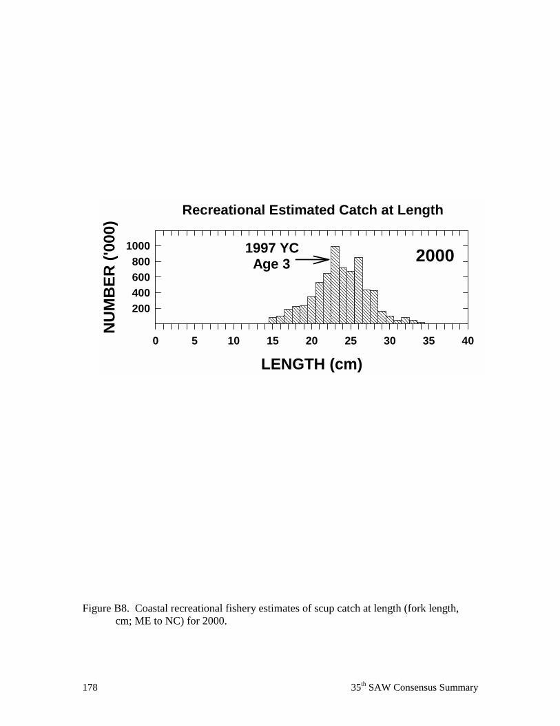
178 35th SAW Consensus Summary
Figure B8. Coastal recreational fishery estimates of scup catch at length (fork length,
cm; ME to NC) for 2000.
Recreational Estimated Catch at Length
LENGTH (cm)0 5 10 15 20 25 30 35 40
NU
MB
ER ('
000)
200400600800
1000 20001997 YC Age 3
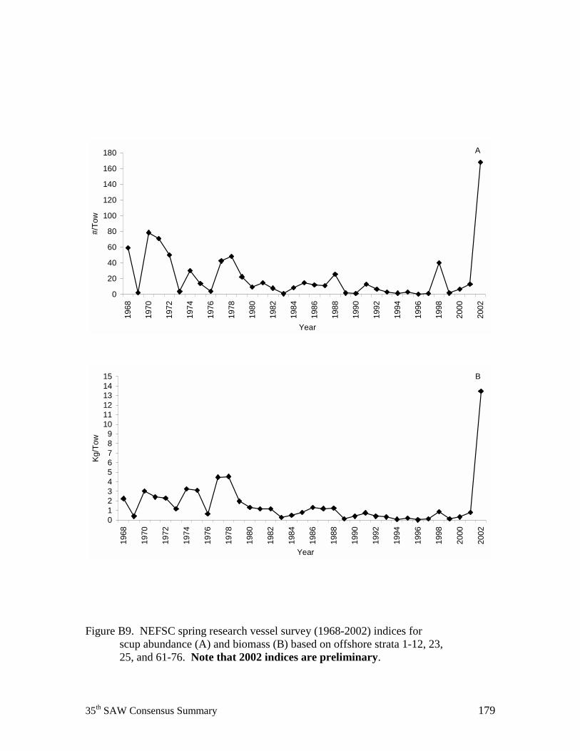
35th SAW Consensus Summary 179
Figure B9. NEFSC spring research vessel survey (1968-2002) indices for
scup abundance (A) and biomass (B) based on offshore strata 1-12, 23, 25, and 61-76. Note that 2002 indices are preliminary.
A
0
20
40
60
80
100
120
140
160
180
1968
1970
1972
1974
1976
1978
1980
1982
1984
1986
1988
1990
1992
1994
1996
1998
2000
2002
Year
#/To
w
B
0123456789
101112131415
1968
1970
1972
1974
1976
1978
1980
1982
1984
1986
1988
1990
1992
1994
1996
1998
2000
2002
Year
Kg/T
ow
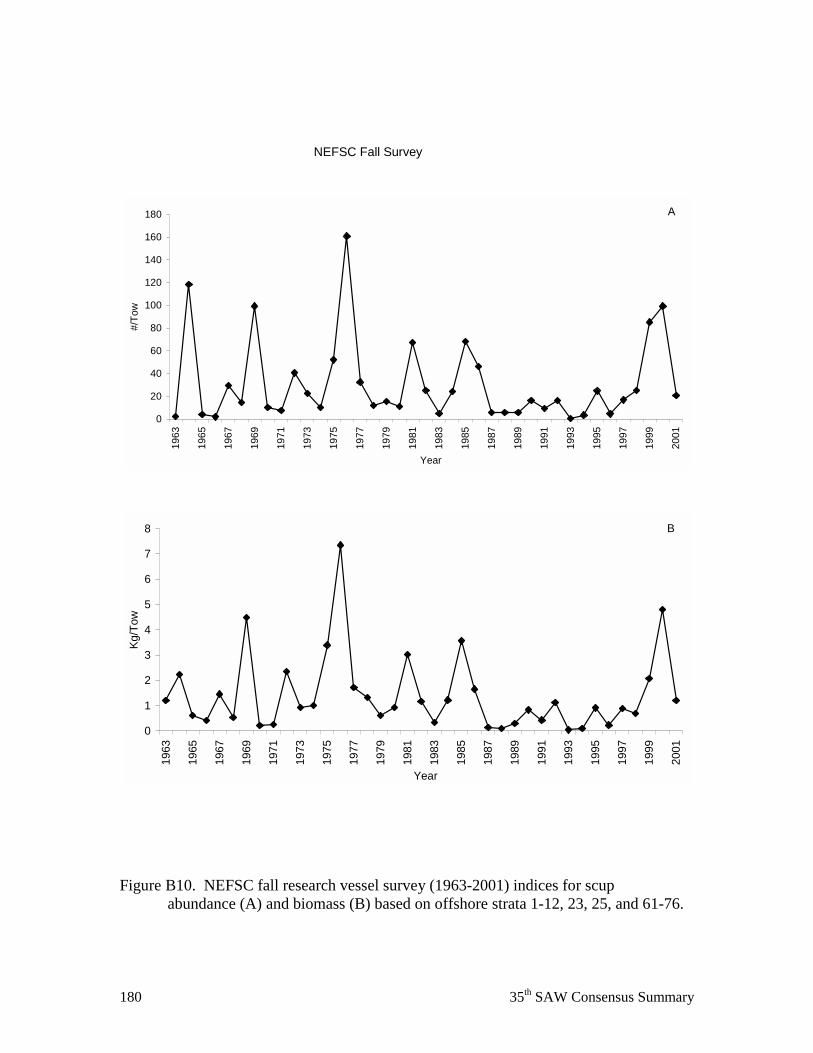
180 35th SAW Consensus Summary
Figure B10. NEFSC fall research vessel survey (1963-2001) indices for scup
abundance (A) and biomass (B) based on offshore strata 1-12, 23, 25, and 61-76.
NEFSC Fall Survey
A
0
20
40
60
80
100
120
140
160
180
1963
1965
1967
1969
1971
1973
1975
1977
1979
1981
1983
1985
1987
1989
1991
1993
1995
1997
1999
2001
Year
#/To
w
B
0
1
2
3
4
5
6
7
8
1963
1965
1967
1969
1971
1973
1975
1977
1979
1981
1983
1985
1987
1989
1991
1993
1995
1997
1999
2001
Year
Kg/T
ow
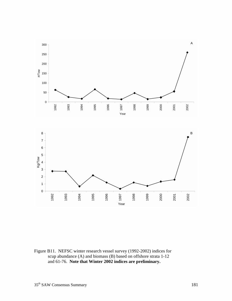
35th SAW Consensus Summary 181
Figure B11. NEFSC winter research vessel survey (1992-2002) indices for
scup abundance (A) and biomass (B) based on offshore strata 1-12 and 61-76. Note that Winter 2002 indices are preliminary.
A
0
50
100
150
200
250
300
1992
1993
1994
1995
1996
1997
1998
1999
2000
2001
2002
Year
#/To
w
B
0
1
2
3
4
5
6
7
8
1992
1993
1994
1995
1996
1997
1998
1999
2000
2001
2002
Year
Kg/T
ow
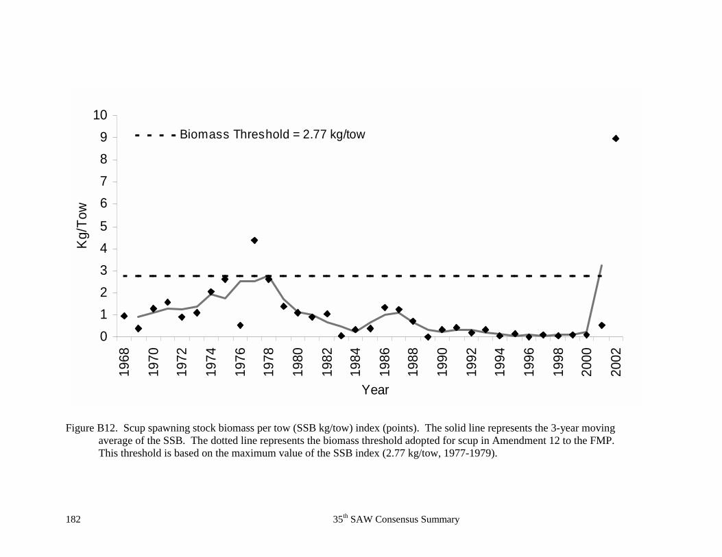
182 35th SAW Consensus Summary
Figure B12. Scup spawning stock biomass per tow (SSB kg/tow) index (points). The solid line represents the 3-year moving
average of the SSB. The dotted line represents the biomass threshold adopted for scup in Amendment 12 to the FMP. This threshold is based on the maximum value of the SSB index (2.77 kg/tow, 1977-1979).
0123456789
1019
68
1970
1972
1974
1976
1978
1980
1982
1984
1986
1988
1990
1992
1994
1996
1998
2000
2002
Year
Kg/
Tow
Biomass Threshold = 2.77 kg/tow
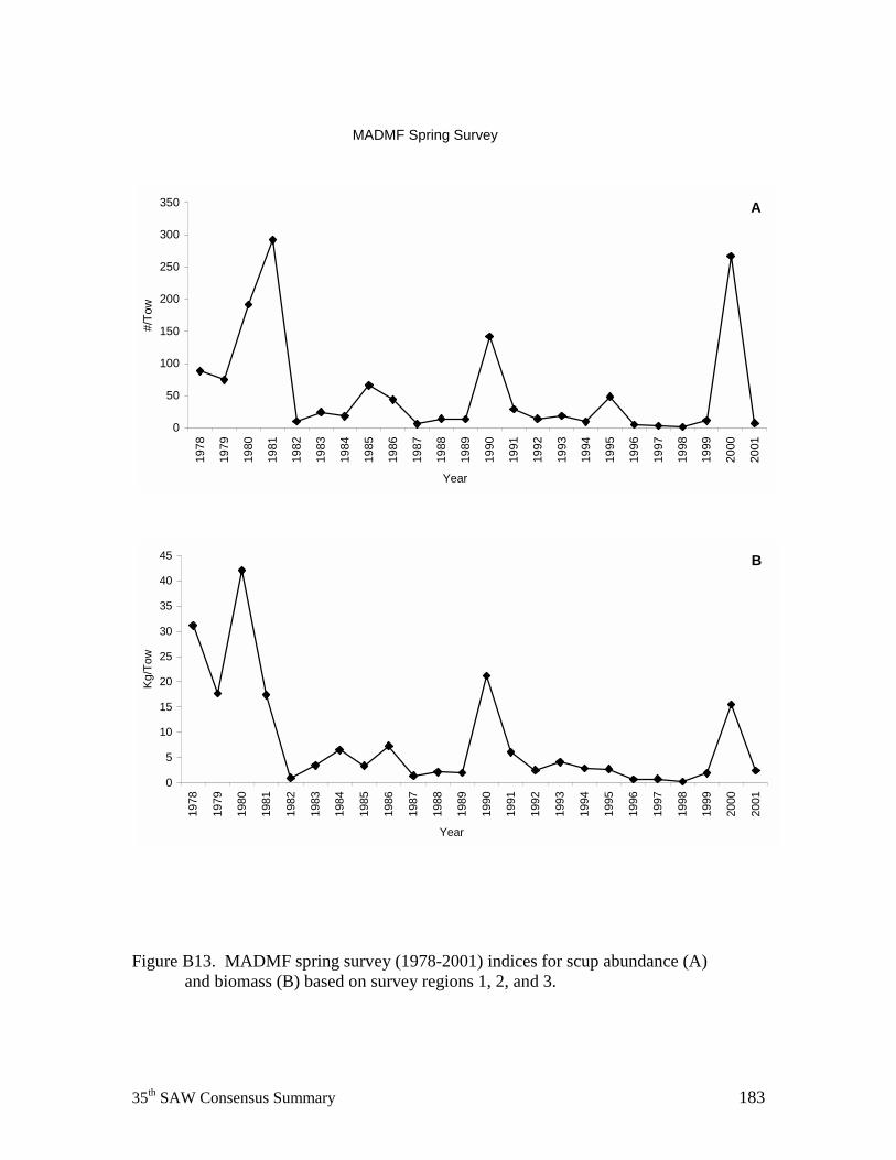
35th SAW Consensus Summary 183
Figure B13. MADMF spring survey (1978-2001) indices for scup abundance (A)
and biomass (B) based on survey regions 1, 2, and 3.
MADMF Spring Survey
A
0
50
100
150
200
250
300
35019
78
1979
1980
1981
1982
1983
1984
1985
1986
1987
1988
1989
1990
1991
1992
1993
1994
1995
1996
1997
1998
1999
2000
2001
Year
#/To
w
B
0
5
10
15
20
25
30
35
40
45
1978
1979
1980
1981
1982
1983
1984
1985
1986
1987
1988
1989
1990
1991
1992
1993
1994
1995
1996
1997
1998
1999
2000
2001
Year
Kg/T
ow
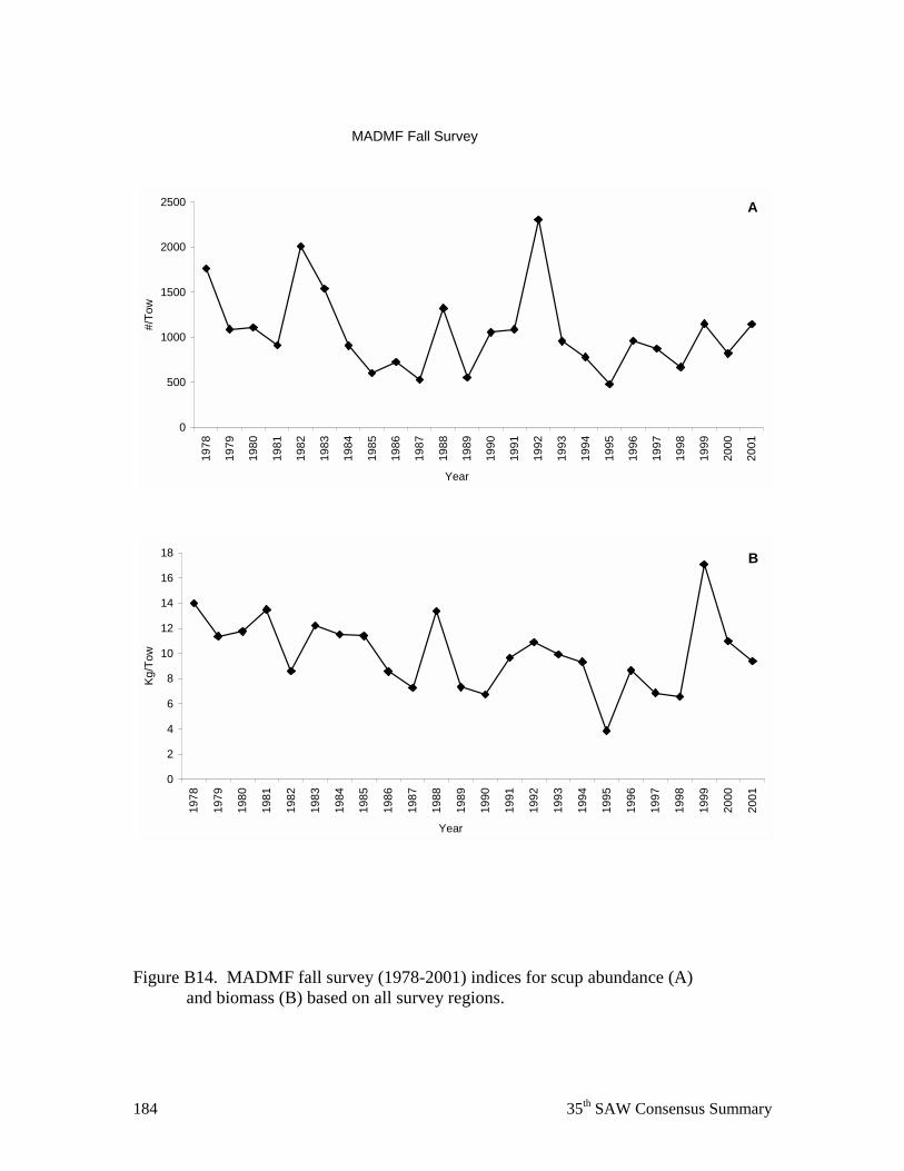
184 35th SAW Consensus Summary
Figure B14. MADMF fall survey (1978-2001) indices for scup abundance (A)
and biomass (B) based on all survey regions.
MADMF Fall Survey
A
0
500
1000
1500
2000
250019
78
1979
1980
1981
1982
1983
1984
1985
1986
1987
1988
1989
1990
1991
1992
1993
1994
1995
1996
1997
1998
1999
2000
2001
Year
#/To
w
B
0
2
4
6
8
10
12
14
16
18
1978
1979
1980
1981
1982
1983
1984
1985
1986
1987
1988
1989
1990
1991
1992
1993
1994
1995
1996
1997
1998
1999
2000
2001
Year
Kg/T
ow
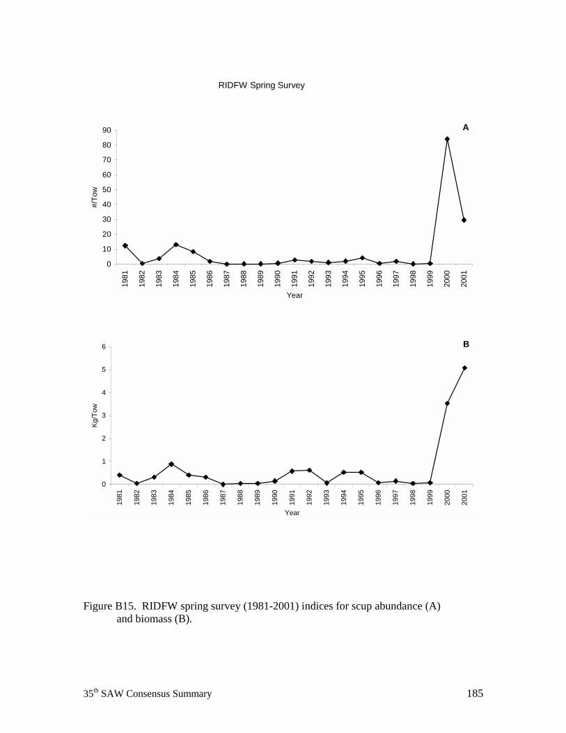
35th SAW Consensus Summary 185
Figure B15. RIDFW spring survey (1981-2001) indices for scup abundance (A)
and biomass (B).
RIDFW Spring Survey
A
0
10
20
30
40
50
60
70
80
9019
81
1982
1983
1984
1985
1986
1987
1988
1989
1990
1991
1992
1993
1994
1995
1996
1997
1998
1999
2000
2001
Year
#/To
w
B
0
1
2
3
4
5
6
1981
1982
1983
1984
1985
1986
1987
1988
1989
1990
1991
1992
1993
1994
1995
1996
1997
1998
1999
2000
2001
Year
Kg/T
ow
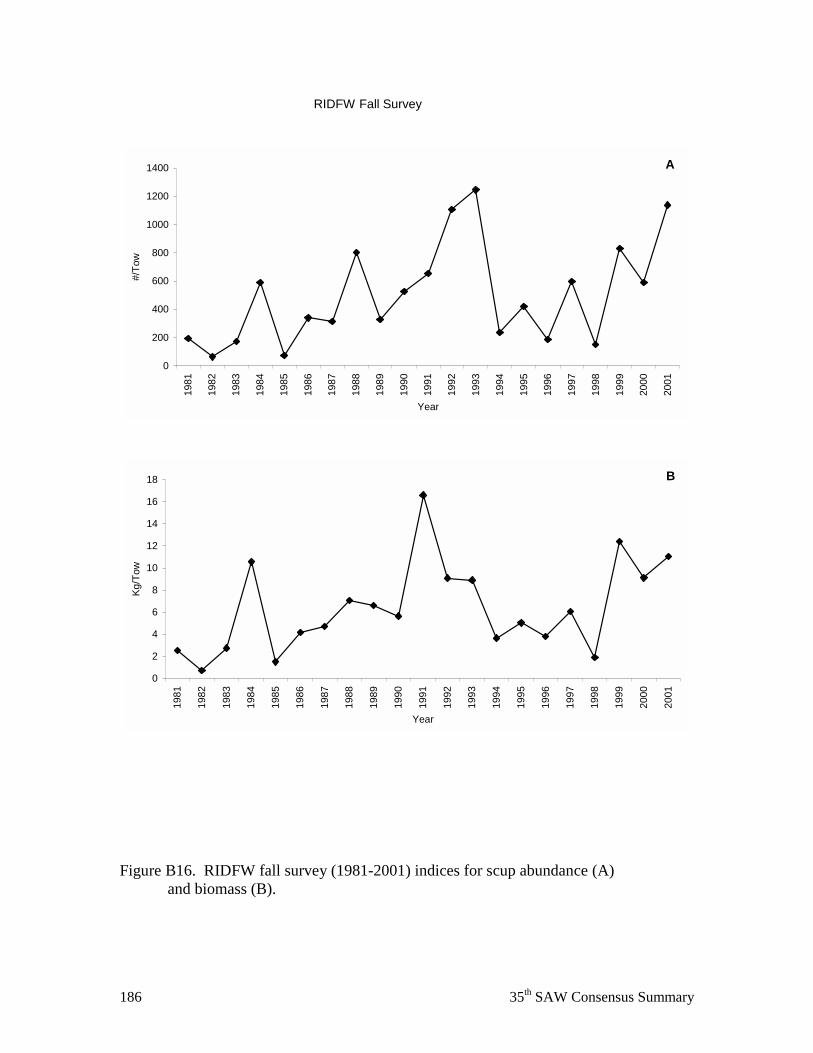
186 35th SAW Consensus Summary
Figure B16. RIDFW fall survey (1981-2001) indices for scup abundance (A)
and biomass (B).
RIDFW Fall Survey
A
0
200
400
600
800
1000
1200
1400
1981
1982
1983
1984
1985
1986
1987
1988
1989
1990
1991
1992
1993
1994
1995
1996
1997
1998
1999
2000
2001
Year
#/To
w
B
0
2
4
6
8
10
12
14
16
18
1981
1982
1983
1984
1985
1986
1987
1988
1989
1990
1991
1992
1993
1994
1995
1996
1997
1998
1999
2000
2001
Year
Kg/T
ow
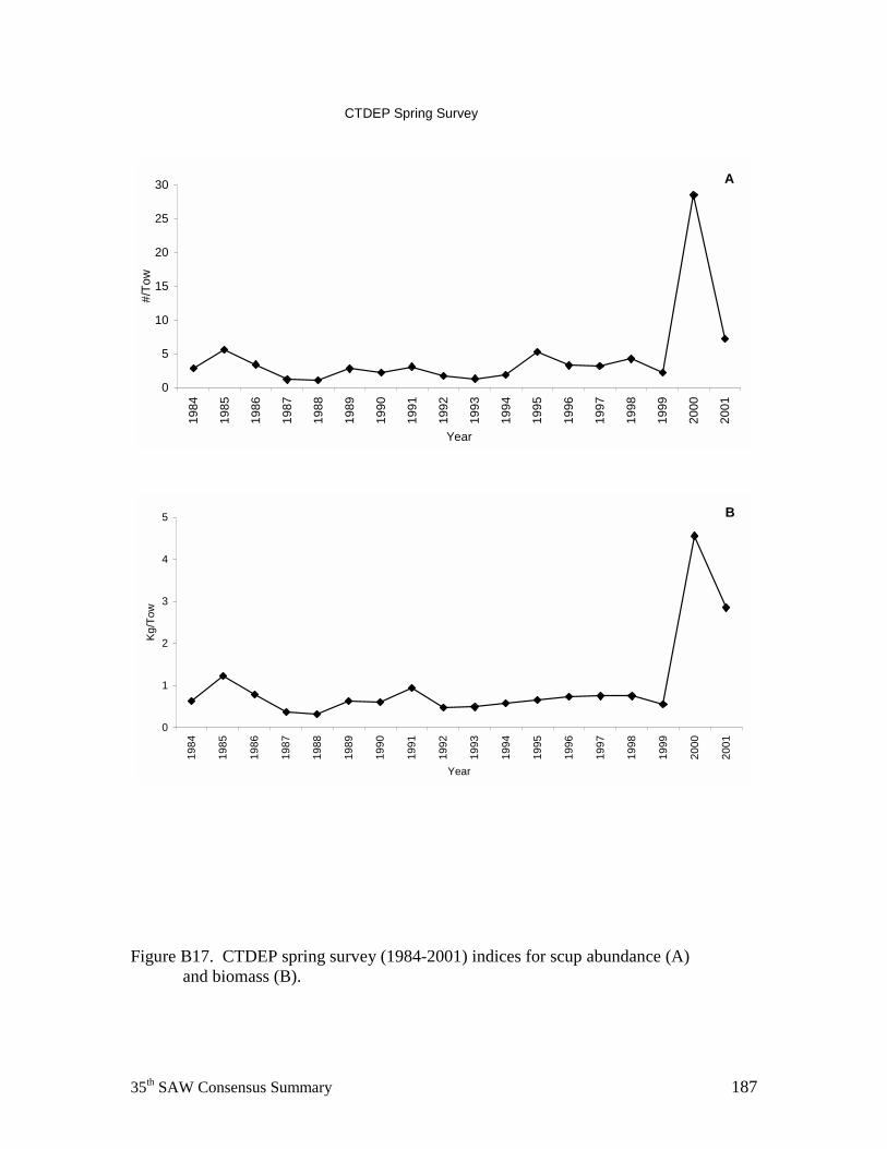
35th SAW Consensus Summary 187
Figure B17. CTDEP spring survey (1984-2001) indices for scup abundance (A)
and biomass (B).
CTDEP Spring Survey
A
0
5
10
15
20
25
3019
84
1985
1986
1987
1988
1989
1990
1991
1992
1993
1994
1995
1996
1997
1998
1999
2000
2001
Year
#/To
w
B
0
1
2
3
4
5
1984
1985
1986
1987
1988
1989
1990
1991
1992
1993
1994
1995
1996
1997
1998
1999
2000
2001
Year
Kg/T
ow
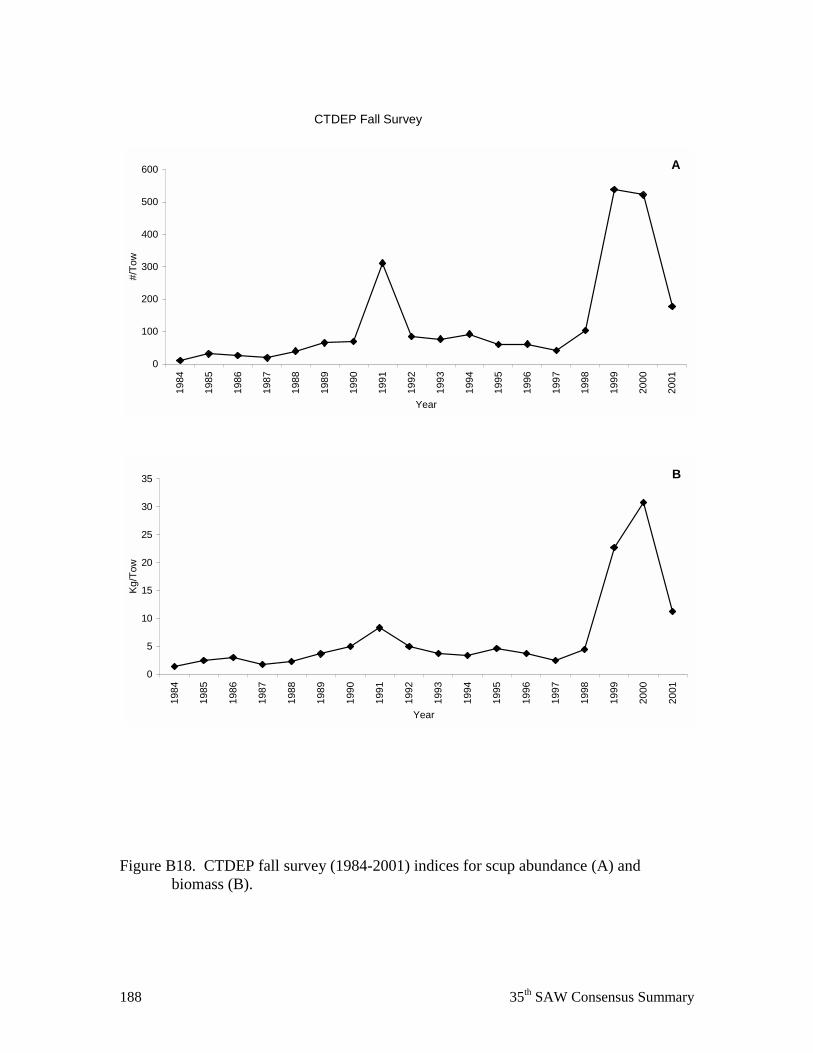
188 35th SAW Consensus Summary
Figure B18. CTDEP fall survey (1984-2001) indices for scup abundance (A) and
biomass (B).
CTDEP Fall Survey
A
0
100
200
300
400
500
60019
84
1985
1986
1987
1988
1989
1990
1991
1992
1993
1994
1995
1996
1997
1998
1999
2000
2001
Year
#/To
w
B
0
5
10
15
20
25
30
35
1984
1985
1986
1987
1988
1989
1990
1991
1992
1993
1994
1995
1996
1997
1998
1999
2000
2001
Year
Kg/T
ow
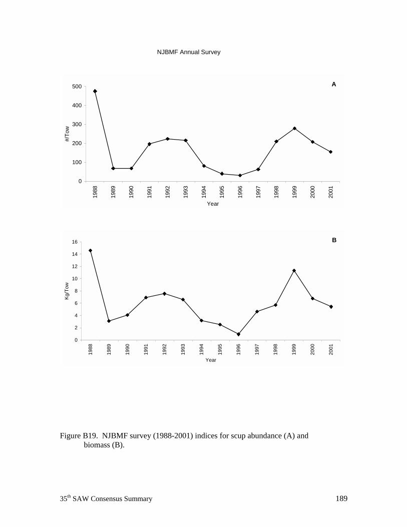
35th SAW Consensus Summary 189
Figure B19. NJBMF survey (1988-2001) indices for scup abundance (A) and
biomass (B).
NJBMF Annual Survey
A
0
100
200
300
400
50019
88
1989
1990
1991
1992
1993
1994
1995
1996
1997
1998
1999
2000
2001
Year
#/To
w
B
0
2
4
6
8
10
12
14
16
1988
1989
1990
1991
1992
1993
1994
1995
1996
1997
1998
1999
2000
2001
Year
Kg/T
ow
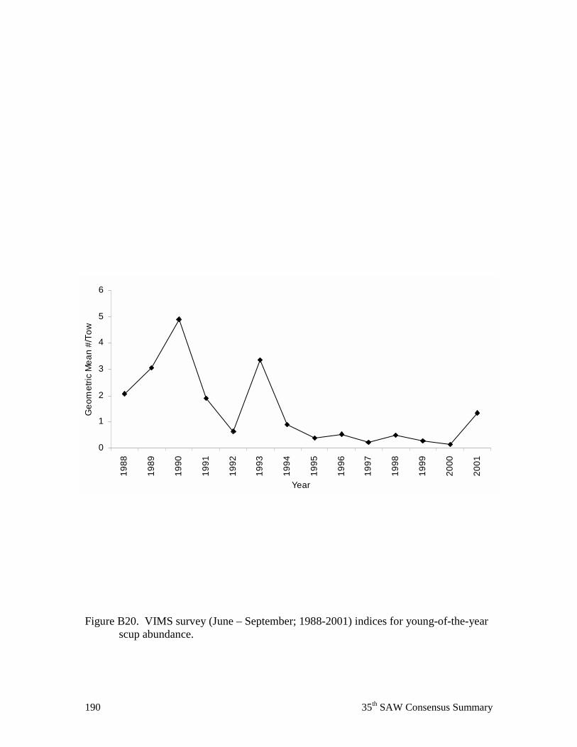
190 35th SAW Consensus Summary
Figure B20. VIMS survey (June – September; 1988-2001) indices for young-of-the-year
scup abundance.
0
1
2
3
4
5
6
1988
1989
1990
1991
1992
1993
1994
1995
1996
1997
1998
1999
2000
2001
Year
Geo
met
ric M
ean
#/To
w
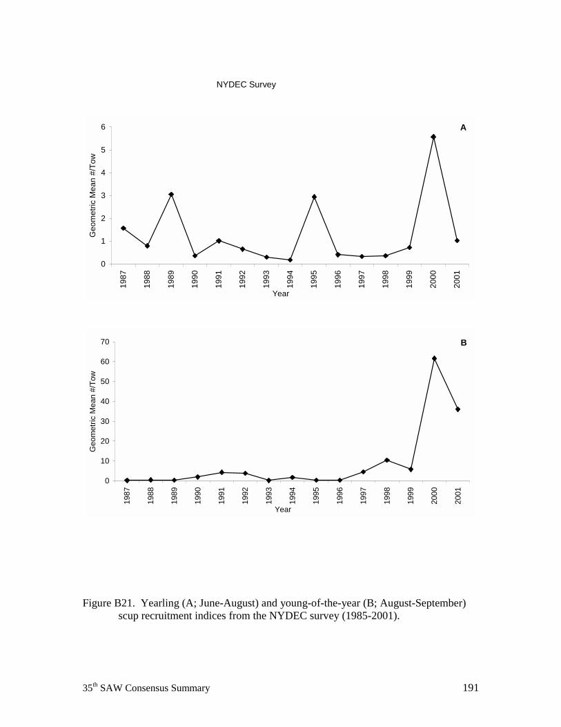
35th SAW Consensus Summary 191
Figure B21. Yearling (A; June-August) and young-of-the-year (B; August-September)
scup recruitment indices from the NYDEC survey (1985-2001).
NYDEC Survey
A
0
1
2
3
4
5
619
87
1988
1989
1990
1991
1992
1993
1994
1995
1996
1997
1998
1999
2000
2001
Year
Geo
met
ric M
ean
#/To
w
B
0
10
20
30
40
50
60
70
1987
1988
1989
1990
1991
1992
1993
1994
1995
1996
1997
1998
1999
2000
2001
Year
Geo
met
ric M
ean
#/To
w

192 35th SAW Consensus Summary
Figure B22. Distribution of scup during NEFSC 1992-1998 spring bottom trawl survey.
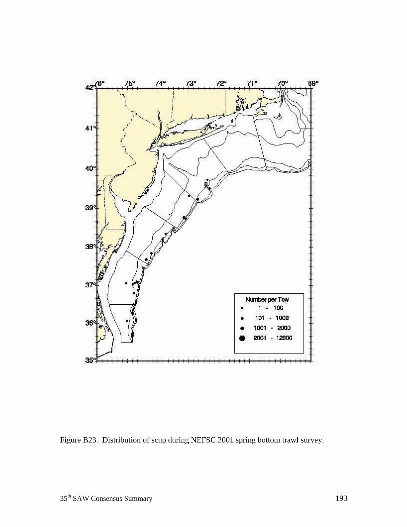
35th SAW Consensus Summary 193
Figure B23. Distribution of scup during NEFSC 2001 spring bottom trawl survey.
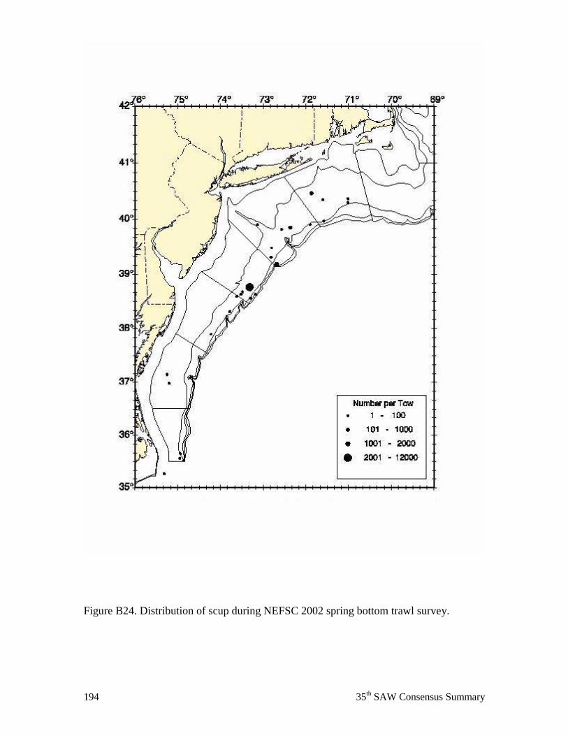
194 35th SAW Consensus Summary
Figure B24. Distribution of scup during NEFSC 2002 spring bottom trawl survey.
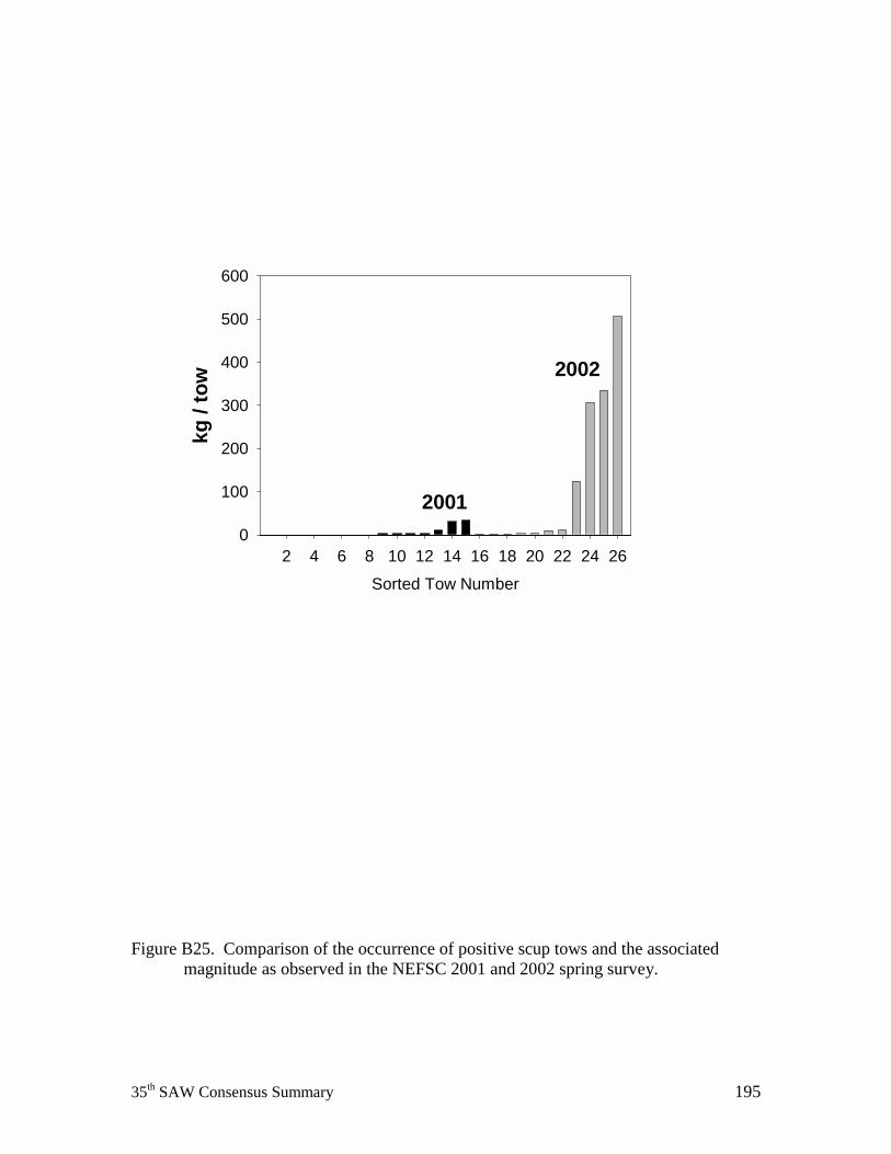
35th SAW Consensus Summary 195
Figure B25. Comparison of the occurrence of positive scup tows and the associated
magnitude as observed in the NEFSC 2001 and 2002 spring survey.
Sorted Tow Number2 4 6 8 10 12 14 16 18 20 22 24 26
kg /
tow
0
100
200
300
400
500
600
2002
2001
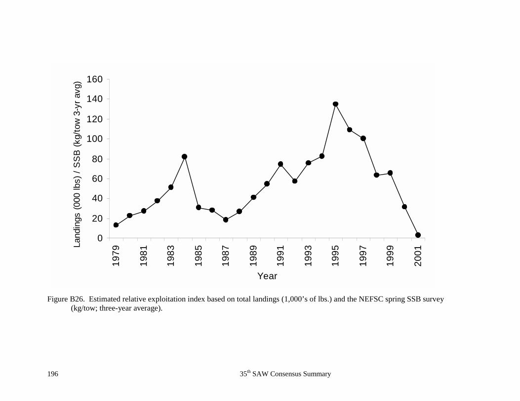
196 35th SAW Consensus Summary
Figure B26. Estimated relative exploitation index based on total landings (1,000’s of lbs.) and the NEFSC spring SSB survey
(kg/tow; three-year average).
0
20
40
60
80
100
120
140
160
1979
1981
1983
1985
1987
1989
1991
1993
1995
1997
1999
2001
Year
Land
ings
(000
lbs)
/ S
SB
(kg/
tow
3-y
r avg
)
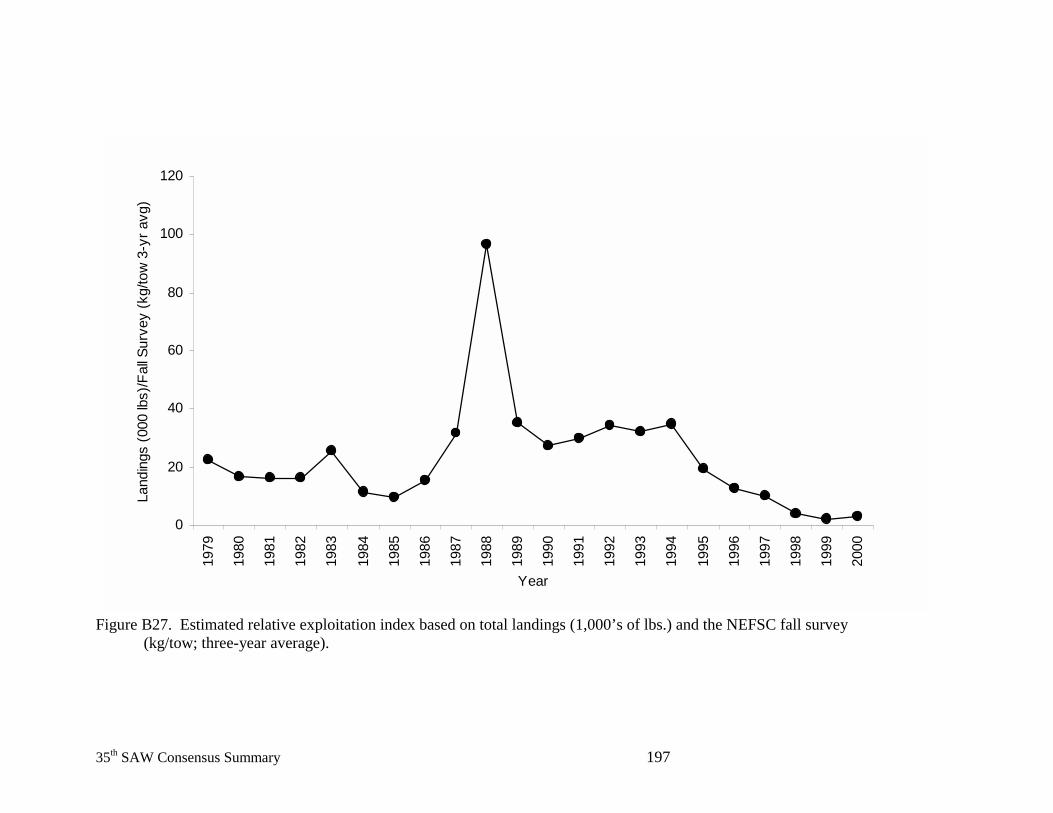
35th SAW Consensus Summary 197
Figure B27. Estimated relative exploitation index based on total landings (1,000’s of lbs.) and the NEFSC fall survey
(kg/tow; three-year average).
0
20
40
60
80
100
120
1979
1980
1981
1982
1983
1984
1985
1986
1987
1988
1989
1990
1991
1992
1993
1994
1995
1996
1997
1998
1999
2000
Year
Land
ings
(000
lbs)
/Fal
l Sur
vey
(kg/
tow
3-y
r avg
)
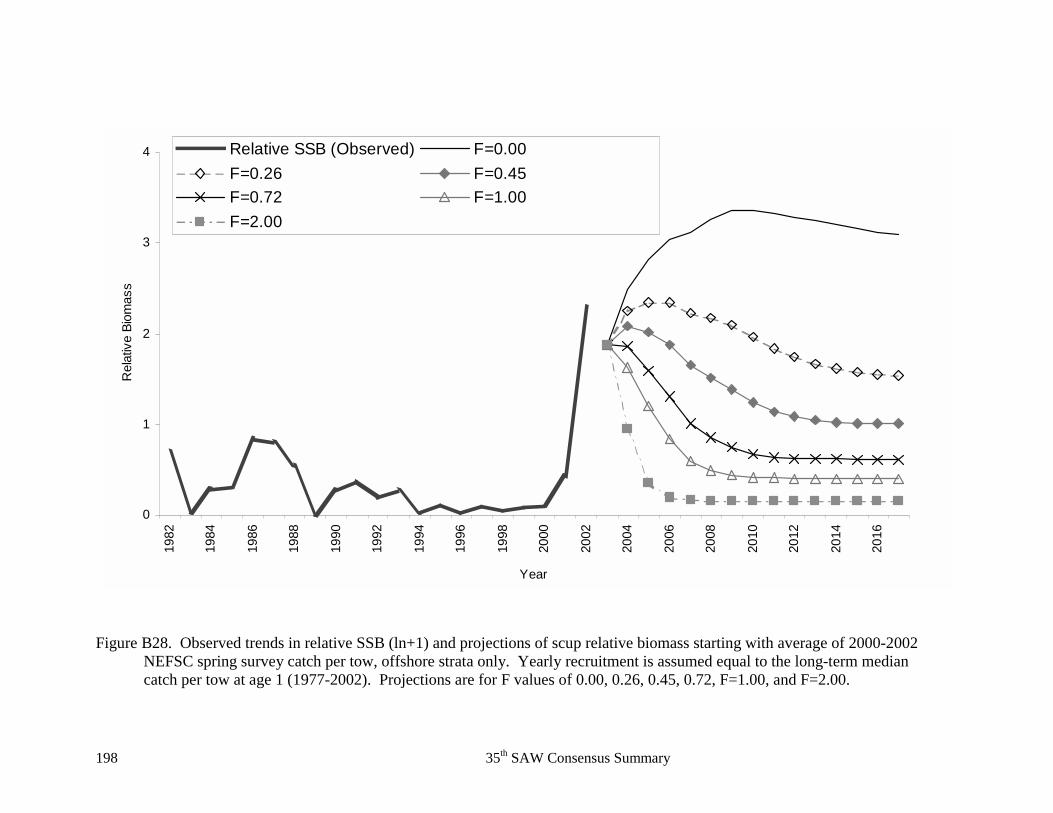
198 35th SAW Consensus Summary
Figure B28. Observed trends in relative SSB (ln+1) and projections of scup relative biomass starting with average of 2000-2002
NEFSC spring survey catch per tow, offshore strata only. Yearly recruitment is assumed equal to the long-term median catch per tow at age 1 (1977-2002). Projections are for F values of 0.00, 0.26, 0.45, 0.72, F=1.00, and F=2.00.
0
1
2
3
419
82
1984
1986
1988
1990
1992
1994
1996
1998
2000
2002
2004
2006
2008
2010
2012
2014
2016
Year
Rel
ativ
e Bi
omas
s
Relative SSB (Observed) F=0.00F=0.26 F=0.45F=0.72 F=1.00F=2.00
35th SAW Consensus Summary 199
C. Application of Index Methods: Catch and Fishery Independent Abundance Surveys
OVERVIEW
Despite an unmatched time series of synoptic research vessel-based surveys, the ability to applyage-based assessment models to marine finfish stocks in the Northeast USA is limited by the number ofyears for which age samples are available. Typically this means that such assessments are restricted to timeperiods beginning in the late 1970's or early 1980's. In many instances, severe overfishing of the resourcehas already occurred, and the information content of the available series may be problematic for theestablishment of biomass reference points. In these situations, it is desirable to apply methods that canincorporate historical catch information, thereby avoiding a myopic perspective on resource conditions.In this report, a number of index-based approaches are developed to more fully utilize the data sets fromthe surveys and historical landings. The methods are technically simple but are based on linear populationmodels, modern graphical methods, and robust statistical models. The concept of a replacement ratio isintroduced here as an analytical tool for examining the historical behavior of a population and any potentialinfluence of removals due to fishing activities.
To test these concepts and to facilitate comparisons, the analyses were applied to both the agedand un-aged stocks. Index-based methods for reference point estimation were considered in light of thespecific goal of identifying the limit relative fishing mortality rate (relF) that is associated with stockreplacement, in the long term. The replacement ratio method was applied to revise estimates of F proxiesfor six stocks: Gulf of Maine haddock, Mid-Atlantic yellowtail flounder, pollock, northern and southernwindowpane, and ocean pout. In some cases, biomass proxies and MSY values were also updated forthese stocks. Catch forecasts are developed for all of the 19 stocks considered as part of the Northeastmultispecies groundfish complex. For a limited number of stocks, index-based forecasts are compared toage-based estimates. The proposed methodology was applied to summer flounder and scup as an adjunctto the analyses prepared by the respective subcommittees for these species for SARC 35.
Index-based approaches can be viewed as important tools for the identification and developmentof parametric models of stock dynamics. Additional simulation work is necessary to support thetheoretical basis for the method and the limits of its applicability.
INTRODUCTION
One of the core problems in fisheries science is the estimation of the scaling factor betweenestimates of relative abundance and true population size. This scaling factor is generally called thecatchability coefficient. Assessment models that rely on VPA utilize the record of age-specific catches toapproximate the virtual population. The utility of the virtual population as a means of estimating catchabilityrests on assumptions that the losses due to fishing are both known and large relative to natural mortality.
200 35th SAW Consensus Summary
Age-structured assessments are data intensive and their scope is restricted to years in which both catchand abundance indices can be aged. Such restrictions can greatly reduce the number of the number ofyears available for analyses. For Northeast USA stocks this often precludes consideration of large-scalereductions in abundance coincident with the presence of distant water fleets in the 1960's and early 1970's.
Reduced-parameter models are often used to analyze non-age structured models. The mostcommon example is the surplus production model (see Prager 1994 for review and modern approaches)but the Collie-Sissenwine model (Collie and Sissenwine 1983), and delay-difference models (Schnute1985) are also candidates. Even these simple models may fail when the dynamic range of populationresponses and/or fishing mortality rates is small (Hilborn and Walters 1993). For example, a time seriescharacterized by continuously declining abundance indices contains relatively little information about theproductive capacity of that stock. Under these circumstances the maximum population biomass (K) isestimable only if it assumed that the initial population size represents an unfished stock. This assumption israrely tenable for Northwest Atlantic stocks that have been fished for hundreds of years and monitoredsince 1960.
The Collie-Sissenwine model replaces a structural model for biomass dynamics with a sequenceof recruitment estimates and simple mass balance equation. The increased parameterization may lead toinstability in the catchability coefficient and therefore, population estimates. As in delay-difference models,poorly specified growth parameters and sampling variability can greatly influence the ability to estimateabundance. Even the simplest parametric models may be difficult to fit to data characterized by largeobservation errors.
In this report we explore the general trends in abundance and fishing mortality deducible from atime series of catch (or landings for some species) and survey indices. For all stocks, only the total catch(mt) and autumn and spring research trawl survey indices (kg/tow) are utilized. We explore the relativefishing mortality rate, defined as the ratio of catch to survey index, and relate it to what we call thereplacement ratio. The replacement ratio is introduced here as an analytical tool for examining the historicalbehavior of a population and any potential influence of removals due to fishing activities. To test theseconcepts and to facilitate comparisons, the analyses were applied to both the aged and un-aged stocks.
REPLACEMENT RATIO THEORY
The replacement ratio draws from the ideas underlying the Sissenwine-Shepherd model, delay-difference models, life-history theory, Collie-Sissenwine model, and statistical smoothing (Simonoff 1996).We begin by defining Ij,s,t as the j-th relative abundance index for species-stock unit s at time t and Cs,t
as the catch (or landings) of species-stock unit s at time t. The simple relative fishing mortality rate withrespect to index type j, stock s and time t is defined as the ratio of Cs,t to Ij,s,t. This ratio can be noisy,owing to imprecision of survey estimates, and the variation can be damped by writing the relative F as a
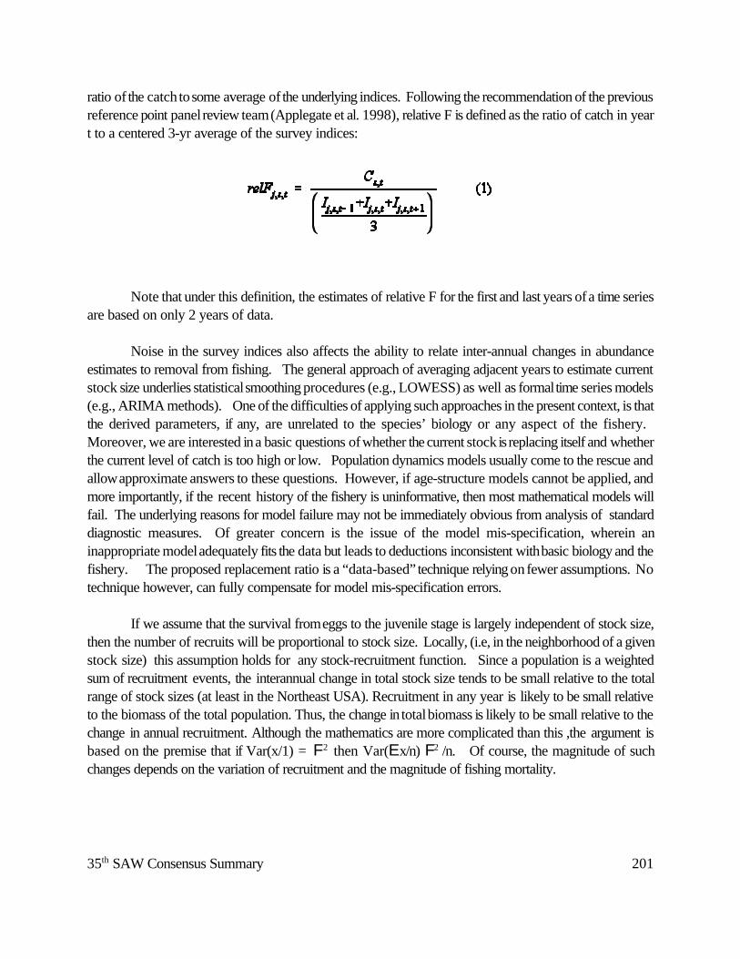
35th SAW Consensus Summary 201
ratio of the catch to some average of the underlying indices. Following the recommendation of the previousreference point panel review team (Applegate et al. 1998), relative F is defined as the ratio of catch in yeart to a centered 3-yr average of the survey indices:
Note that under this definition, the estimates of relative F for the first and last years of a time seriesare based on only 2 years of data.
Noise in the survey indices also affects the ability to relate inter-annual changes in abundanceestimates to removal from fishing. The general approach of averaging adjacent years to estimate currentstock size underlies statistical smoothing procedures (e.g., LOWESS) as well as formal time series models(e.g., ARIMA methods). One of the difficulties of applying such approaches in the present context, is thatthe derived parameters, if any, are unrelated to the species’ biology or any aspect of the fishery. Moreover, we are interested in a basic questions of whether the current stock is replacing itself and whetherthe current level of catch is too high or low. Population dynamics models usually come to the rescue andallow approximate answers to these questions. However, if age-structure models cannot be applied, andmore importantly, if the recent history of the fishery is uninformative, then most mathematical models willfail. The underlying reasons for model failure may not be immediately obvious from analysis of standarddiagnostic measures. Of greater concern is the issue of the model mis-specification, wherein aninappropriate model adequately fits the data but leads to deductions inconsistent with basic biology and thefishery. The proposed replacement ratio is a “data-based” technique relying on fewer assumptions. Notechnique however, can fully compensate for model mis-specification errors.
If we assume that the survival from eggs to the juvenile stage is largely independent of stock size,then the number of recruits will be proportional to stock size. Locally, (i.e, in the neighborhood of a givenstock size) this assumption holds for any stock-recruitment function. Since a population is a weightedsum of recruitment events, the interannual change in total stock size tends to be small relative to the totalrange of stock sizes (at least in the Northeast USA). Recruitment in any year is likely to be small relativeto the biomass of the total population. Thus, the change in total biomass is likely to be small relative to thechange in annual recruitment. Although the mathematics are more complicated than this ,the argument isbased on the premise that if Var(x/1) = F2 then Var(Ex/n) F2 /n. Of course, the magnitude of suchchanges depends on the variation of recruitment and the magnitude of fishing mortality.
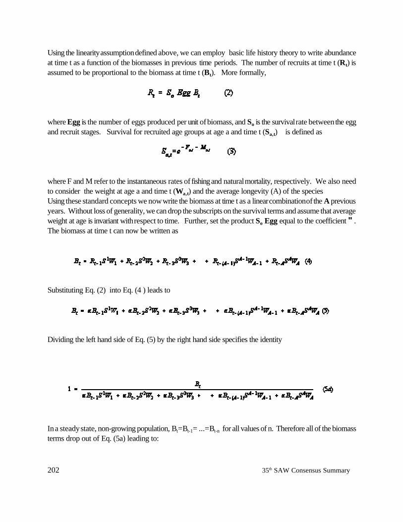
202 35th SAW Consensus Summary
Using the linearity assumption defined above, we can employ basic life history theory to write abundanceat time t as a function of the biomasses in previous time periods. The number of recruits at time t (Rt) isassumed to be proportional to the biomass at time t (Bt). More formally,
where Egg is the number of eggs produced per unit of biomass, and So is the survival rate between the eggand recruit stages. Survival for recruited age groups at age a and time t (Sa,t) is defined as
where F and M refer to the instantaneous rates of fishing and natural mortality, respectively. We also needto consider the weight at age a and time t (Wa,t) and the average longevity (A) of the species Using these standard concepts we now write the biomass at time t as a linear combination of the A previousyears. Without loss of generality, we can drop the subscripts on the survival terms and assume that averageweight at age is invariant with respect to time. Further, set the product So Egg equal to the coefficient " .The biomass at time t can now be written as
Substituting Eq. (2) into Eq. (4 ) leads to
Dividing the left hand side of Eq. (5) by the right hand side specifies the identity
In a steady state, non-growing population, Bt=Bt-1= ...=Bt-n for all values of n. Therefore all of the biomassterms drop out of Eq. (5a) leading to:
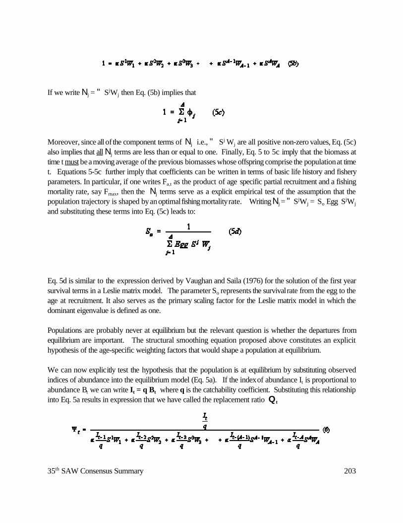
35th SAW Consensus Summary 203
If we write Nj = " SjWj then Eq. (5b) implies that
Moreover, since all of the component terms of Nj i.e., " Sj Wj are all positive non-zero values, Eq. (5c)also implies that all Nj terms are less than or equal to one. Finally, Eq. 5 to 5c imply that the biomass attime t must be a moving average of the previous biomasses whose offspring comprise the population at timet. Equations 5-5c further imply that coefficients can be written in terms of basic life history and fisheryparameters. In particular, if one writes Fa,t as the product of age specific partial recruitment and a fishingmortality rate, say Fmax, then the Nj terms serve as a explicit empirical test of the assumption that thepopulation trajectory is shaped by an optimal fishing mortality rate. Writing Nj = " SjWj = So Egg SjWj
and substituting these terms into Eq. (5c) leads to:
Eq. 5d is similar to the expression derived by Vaughan and Saila (1976) for the solution of the first yearsurvival terms in a Leslie matrix model. The parameter So represents the survival rate from the egg to theage at recruitment. It also serves as the primary scaling factor for the Leslie matrix model in which thedominant eigenvalue is defined as one.
Populations are probably never at equilibrium but the relevant question is whether the departures fromequilibrium are important. The structural smoothing equation proposed above constitutes an explicithypothesis of the age-specific weighting factors that would shape a population at equilibrium.
We can now explicitly test the hypothesis that the population is at equilibrium by substituting observedindices of abundance into the equilibrium model (Eq. 5a). If the index of abundance It is proportional toabundance Bt we can write It = q Bt where q is the catchability coefficient. Substituting this relationshipinto Eq. 5a results in expression that we have called the replacement ratio Qt
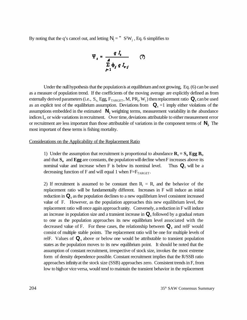
204 35th SAW Consensus Summary
By noting that the q’s cancel out, and letting Nj = " SjWj , Eq. 6 simplifies to
Under the null hypothesis that the population is at equilibrium and not growing, Eq. (6) can be usedas a measure of population trend. If the coefficients of the moving average are explicitly defined as fromexternally derived parameters (i.e., So, Egg, FTARGET, M, PRj, Wj ) then replacement ratio Qt can be usedas an explicit test of the equilibrium assumption. Deviations from Qt =1 imply either violations of theassumptions embedded in the estimated Nj weighting terms, measurement variability in the abundanceindices It, or wide variations in recruitment. Over time, deviations attributable to either measurement erroror recruitment are less important than those attributable of variations in the component terms of Nj. Themost important of these terms is fishing mortality.
Considerations on the Applicability of the Replacement Ratio
1) Under the assumption that recruitment is proportional to abundance Rt = So Egg Bt,and that So and Egg are constants, the population will decline when F increases above itsnominal value and increase when F is below its nominal level. Thus Qt will be adecreasing function of F and will equal 1 when F=FTARGET.
2) If recruitment is assumed to be constant then Rt = R, and the behavior of thereplacement ratio will be fundamentally different. Increases in F will induce an initialreduction in Qt as the population declines to a new equilibrium level consistent increasedvalue of F. However, as the population approaches this new equilibrium level, thereplacement ratio will once again approach unity. Conversely, a reduction in F will inducean increase in population size and a transient increase in Qt followed by a gradual returnto one as the population approaches its new equilibrium level associated with thedecreased value of F. For these cases, the relationship between Q t and relF wouldconsist of multiple stable points. The replacement ratio will be one for multiple levels ofrelF. Values of Q t above or below one would be attributable to transient populationstates as the population moves to its new equilibrium point. It should be noted that theassumption of constant recruitment, irrespective of stock size, invokes the most extremeform of density dependence possible. Constant recruitment implies that the R/SSB ratioapproaches infinity at the stock size (SSB) approaches zero. Consistent trends in F, fromlow to high or vice versa, would tend to maintain the transient behavior in the replacement
35th SAW Consensus Summary 205
ratio for longer periods. Therefore, the relationship between Qt and relative F wouldapproximate that observed in paragraph 1).
3) The behavior of the replacement ratio in situations where the underlying stockrecruitment function invokes varying degrees of compensation (say a Beverton-Holtrelation), will be intermediate between behaviors described in paragraphs 1) and 2) above.If the stock is near carrying capacity then deviations from an average level of recruitmentwill be small. For this situation, the behavior of the replacement ratio will be similar to thatdescribed in paragraph 2). When the population is small relative to the level that producesmaximum or near maximum levels of recruitment, the behavior of Qt and its relationshipto relative F should be similar to that described in paragraph 1). The ability to distinguishbetween the behaviors in Qt induced by simultaneous changes in F or constancy inrecruitment (as the population increases toward some designated level), will be difficult.
4) Many, if not most, of the stocks in the Northeast are at relatively low levels ofabundance and have experienced, until recently, extended periods of increasing fishingmortality. If the populations are controlled by some form of density-dependent stockrecruitment function, it is likely that the recruitment is nearly linear in the vicinity of thecurrent stock size. Under these conditions it is expected that the relationship between Qt
and relF should be similar to that described in paragraph 1).
5) For stocks that are approaching carrying capacity or the some value at whichrecruitment becomes nearly constant (e.g., Georges Bank yellowtail flounder), the utilityof the derived value of the relF at replacement is compromised. In this circumstance, apiecewise examination of the data may be instructive.
Appropriate Number of Terms in Moving AverageThe survival term Sj is equivalent to the lx term in the Euler-Lotka equation for population growth
(lx is the probability of surviving to age x). For high levels of fishing mortality the Sj term is decreasingfaster than the average weight Wj is increasing. Thus the importance of earlier indices rapidly diminishes. All of the It and Nj terms are positive, and at equilibrium, It=It+1 and It =G Nj It-j both hold. Therefore,G Nj = 1 and all of the Nj >0 . It would be desirable to express each of the Nj weighting terms asfunction of the underlying population parameters. As expected, increases in fishing mortality increase theweight to more recent indices, whereas the converse hold for lower fishing mortality rates. As anapproximation for this initial analyses, we assumed that all of the Nj = N which implies that N = 1/A.
Given the high rate of fishing mortality observed in Northeast stocks, we further assumed that A=5was a valid approximation. Note that even moderate levels of fishing mortality imply low Nj valuesbeyond the fifth term. (e.g., F=0.5, M=0.2 imply S5 = 0.03. For the fifth to be important the ratio of theweights between the youngest and oldest ages would have to be greater than 1/S5 which, for this example,
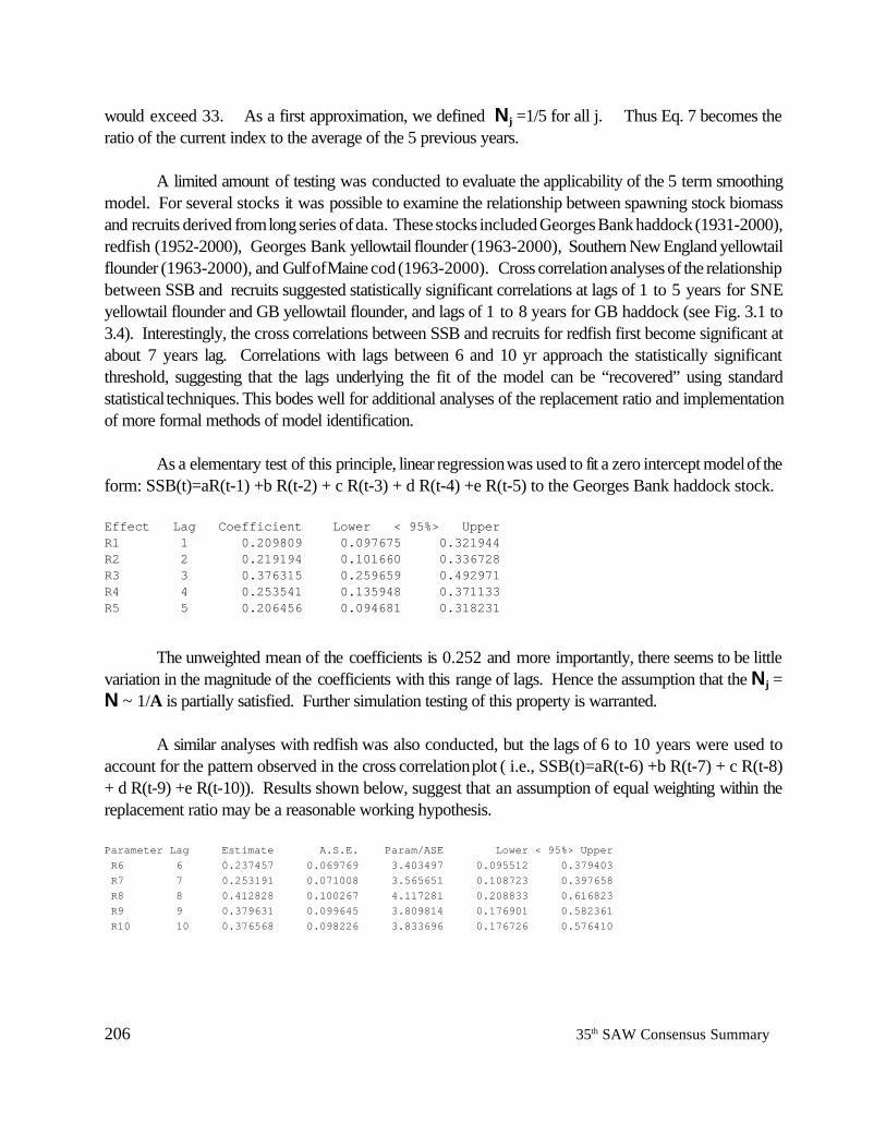
206 35th SAW Consensus Summary
would exceed 33. As a first approximation, we defined Nj =1/5 for all j. Thus Eq. 7 becomes theratio of the current index to the average of the 5 previous years.
A limited amount of testing was conducted to evaluate the applicability of the 5 term smoothingmodel. For several stocks it was possible to examine the relationship between spawning stock biomassand recruits derived from long series of data. These stocks included Georges Bank haddock (1931-2000),redfish (1952-2000), Georges Bank yellowtail flounder (1963-2000), Southern New England yellowtailflounder (1963-2000), and Gulf of Maine cod (1963-2000). Cross correlation analyses of the relationshipbetween SSB and recruits suggested statistically significant correlations at lags of 1 to 5 years for SNEyellowtail flounder and GB yellowtail flounder, and lags of 1 to 8 years for GB haddock (see Fig. 3.1 to3.4). Interestingly, the cross correlations between SSB and recruits for redfish first become significant atabout 7 years lag. Correlations with lags between 6 and 10 yr approach the statistically significantthreshold, suggesting that the lags underlying the fit of the model can be “recovered” using standardstatistical techniques. This bodes well for additional analyses of the replacement ratio and implementationof more formal methods of model identification.
As a elementary test of this principle, linear regression was used to fit a zero intercept model of theform: SSB(t)=aR(t-1) +b R(t-2) + c R(t-3) + d R(t-4) +e R(t-5) to the Georges Bank haddock stock.
Effect Lag Coefficient Lower < 95%> UpperR1 1 0.209809 0.097675 0.321944 R2 2 0.219194 0.101660 0.336728 R3 3 0.376315 0.259659 0.492971 R4 4 0.253541 0.135948 0.371133 R5 5 0.206456 0.094681 0.318231
The unweighted mean of the coefficients is 0.252 and more importantly, there seems to be littlevariation in the magnitude of the coefficients with this range of lags. Hence the assumption that the Nj =N ~ 1/A is partially satisfied. Further simulation testing of this property is warranted.
A similar analyses with redfish was also conducted, but the lags of 6 to 10 years were used toaccount for the pattern observed in the cross correlation plot ( i.e., SSB(t)=aR(t-6) +b R(t-7) + c R(t-8)+ d R(t-9) +e R(t-10)). Results shown below, suggest that an assumption of equal weighting within thereplacement ratio may be a reasonable working hypothesis.
Parameter Lag Estimate A.S.E. Param/ASE Lower < 95%> Upper R6 6 0.237457 0.069769 3.403497 0.095512 0.379403 R7 7 0.253191 0.071008 3.565651 0.108723 0.397658 R8 8 0.412828 0.100267 4.117281 0.208833 0.616823 R9 9 0.379631 0.099645 3.809814 0.176901 0.582361 R10 10 0.376568 0.098226 3.833696 0.176726 0.576410
35th SAW Consensus Summary 207
RELATION BETWEEN REPLACEMENT RATIO AND RELATIVE F
Application of any smoothing technique reflects a choice between signal and noise (Rago 2001)A greater degree of smoothing eliminates the noise but may fail to detect true changes in the signal. Giventhe abrupt changes in fishing mortality that have occurred in some Northeast stocks, we chose to utilize thecurrent year in the numerator of the replacement ratio. Use of the current index in the numerator rather thana running average of say k years, increases the sensitivity of the ratio to detect such changes. The penaltyfor such sensitivity is that the proportions of false positives and false negative responses increase. Thispenalty was judged acceptable for two reasons. First, it is desirable to detect abrupt changes in resourcecondition given the magnitude of recent and proposed management regulations. Second, the currentformulation of the replacement ratio has a natural relationship to stock-recruitment hypotheses and the ratiocan be investigated as a function of variations in underlying parameters, especially survival. Alternativeformulations of the replacement ratio, say with a 2-yr average population size in the numerator can bedeveloped, but their basic properties have not been investigated.
When fishing mortality rates exceed the capacity of the stock to replace itself the population isexpected to decline over time. The expected behavior of Qt under varying fishing mortality andrecruitment is complicated, but it will have a stable point = 1 when the fishing mortality rate is in balancewith recruitment and growth. Variations in fishing mortality will induce complex patterns, but in generalterms, Qt will exceed 1 when relative F is too high, and will be below 1 when F is too low. To accountfor these general properties and to reduce the influence of wide changes in either Qt or the relative F, weapplied robust regression methods (Goodall 1983) to estimate the relative F corresponding to Qt =1. The parameters of the regression model were estimated by
minimizing the median absolute deviations. Median Absolute Deviation estimators are known as MADestimators in the statistical literature (eg. Mosteller and Tukey 1977). Residuals were down weighted usinga bisquare distribution in which the sum of the MAD standardized residuals was set to 6. This roughlycorresponds to a rejection point of about plus or minus two standard deviations from the mean. (Goodall1983).
The relative F at which Qt = 1 was estimated from Eq. 8. as
208 35th SAW Consensus Summary
where the estimates of a and b from Eq. 8 were substituted into Eq. 9. This derived quantity may beappropriately labeled as a threshold since values in excess of it are expected to lead to decliningpopulations. Alternatively, populations are expect to increase when relFt < relFthreshold . Employing thegeneral standard that managers should attempt to rebuild fish stocks within 10 years, we estimated therelative fishing mortality rate at which the expected value of Qt = 1.1 as a measure of relF target. Applyinga little algebra to the Eq. 8 leads to the following estimator of relFtarget:
The asymptotic standard errors of relFthreshold and relFtarget were derived from the Hessian matrix of theregression model.
RANDOMIZATION TESTS
The usual tests of statistical significance do not apply for the model described in Eq. 8. The relationbetween Qt and relFt is of the general form of Y/X vs X where X and Y are random variables. Theexpected correlation between Y/X and X is less than zero and is the basis for the oft stated criticism ofspurious correlation. To test for spurious correlation we developed a sampling distribution of thecorrelation statistic using a randomization test. The randomization test is based on the null hypothesis thatthe catch and survey time series represent a random ordering of observations with no underlyingassociation. The randomization test was developed as follows:
1. Create a random time series of length T of Cr,t from the set {Ct} and Ir,t from the set {It} bysampling with replacement.
2. Compute a random time series of relative F (relFr,t) and replacement ratios ( Qr,t )3. Compute the r-th correlation coefficient, say Dr between ln(relFr,t) and ln( Qr,t ).4. Repeat steps 1 to 3 1000 times.5. Compare the observed correlation coefficient robs with the sorted set of Dr 6. The approximate significance level of the observed correlation coefficient robs is the fraction of
values of Dr less than robs
It should be emphasized that relF is not necessarily an adequate proxy for Fmsy, since this parameter onlyestimates the average mortality rate at which the stock was capable of replacing itself. Thus, while relFdefined as average replacement fishing mortality is a necessary condition for an Fmsy proxy, it is notsufficient, since the stock could theoretically be brought to the stable point under an infinite array of biomassstates.
35th SAW Consensus Summary 209
Even with an estimate of relF derived from the above procedure, externally-derived estimates of Bmsy orMSY are necessary in order to develop consistent estimates of all the management reference points: MSY,Bmsy and Fmsy or their proxies. For index-based assessments these terms are related by
MSY/IBmsy = relF
where IBmsy is the survey index associated with Bmsy. Knowledge of any two of these terms allows forestimation of the third. For some index stocks (e.g. Gulf of Maine haddock) an external estimate of MSYwas considered, based on average catches over a stable period. For others, the IBmsy proxy wasconsidered more reliable.
GRAPHICAL ANALYSES
The six panel plot developed for the “index” species attempts to show the interrelationships amongsurvey estimates of abundance, landings, functions of landings and relative abundance, and time. The twofunctions of landings and relative abundance considered are the replacement ratio (Eq. 6, section 3.0) andrelative F (Eq. 9, section 4.0). The concept of using multiple panels to relate multiple variables over timehas been advocated for use in fisheries science (e.g . Clark 1976, Hilborn and Walters 1992) and otherfields (e.g. Cleveland 1993). The 6-panel plots attempt to show the logical connections among variablesand to estimate underlying biological rates. The example for GOM Haddock (Fig. 6.1) will be discussedin detail here.
The first aspect to note about the plots are the shared axes in the top four plots (A. B., C, D) andF. Panels B , D and F show the time series for the replacement ratio, the fall survey index, and the relativeF, respectively. The horizontal line in A and B is the replacement ratio =1 line. The relationship betweenthe replacement ratio and relative F in panel A is the key to understanding the influence of fishing mortalityon stock size. Panel A is a phase plane that describes the relationship between two variables ordered bytime. The degree of association between these variables is characterized by a Gaussian bivariate ellipsoidwith a nominal probability level of p=0.6827 equivalent to + 1 SD about the mean of the x and y variables.The primary and secondary axes of the ellipse are the first and second principal components, respectively. When the degree of association between relative F and replacement ratio decreases, the ellipse becomesmore circle-like. The implication is that either the survey is too imprecise to detect changes induced byhistorical levels of fishing removals, or that the levels of fishing effort have been too low to effect changesin relative abundance. These alternatives can often be distinguished by consideration of the sampling gearand its interaction with the behavior of the species. Similarly incompleteness of the catch record, particularlyfor species in which the magnitude of discard mortality has varied widely, is another critical factor in theinterpretation of the confidence ellipse.
210 35th SAW Consensus Summary
The assumption that the relative F and replacement ratio have a joint bivariate normal distributionin the log –log scale may not hold for all (or any) species. In particular, the replacement ratio model isdesigned to be sensitive to contemporary changes, so that by definition it will be highly variable. Largechanges that are subsequently validated by future observations imply true changes in population status.When the converse is true, it is proper to conclude that the change was an artifact of sampling variation. The degree to which high residuals influence the pattern is tested using the robust regression method ofTukey (Mosteller and Tukey 1977) that downweights large residuals using a bisquare distribution (seeGoodall 1983 for details). Thus the regression line in panel A will not be aligned with the primary axis ofthe ellipse when high residuals distort the confidence ellipse. The expected value of correlation betweenthe replacement rate and relative F is negative. The empirically derived estimate of the sampling distributionfor the correlation coefficient , via the randomization test, provides a way of judging the significance of therobust regression line.
The predicted value of relative F at which the replacement ratio is 1 is defined by Eq. 8 anddenoted by the vertical line in Panel A and B. The precision of that point depends largely upon where itlies within the confidence ellipse. If the confidence ellipse is nearly centered about the intersection point,then the precision of the relative F threshold will be high. This also indicates that over time, a wide rangeof F and replacement ratios greater than one have been observed. In contrast, when the intersection pointlies in the upper right portion of ellipse, the precision will be low. This is, of course, is a common propertyof linear regression in which the prediction interval for Y increases with the square of the distance betweenthe independent variable X and its mean. Thus a high degree of correlation between relative F and thereplacement ratio does not necessarily ensure high precision in the threshold if relatively few observationshave replacement ratios greater than one. Panel A demonstrates, in a slightly different way, the implicationsof the “one-way trip” described in Hilborn and Walters (1992)
Panel C depicts the phase plane for relative biomass (i.e., . The index) and the relative F. Atequilibrium, the population should move up and down a linear isocline. The degree of departure fromlinearity reflects both sampling variation as well as true variations induced by recruitment pulses and itstransient influence on total biomass. Thus the trace of points can give useful insights into parametric modelselection of population dynamics under exploitation .
The simple data of catch and survey are generally not sufficient to estimate simultaneously both thethreshold F and biomass targets. This property characterizes the common property of indeterminancy ofr and K in standard surplus production models. For the GOM haddock example, the relative biomasstarget is defined external to the model (Panel C and D).
To facilitate the detection of temporal patterns, Lowess smoothing is applied in panels B, D, andF. A relatively low tension =0.3 (i.e., 30% of the span of data are used for the estimate of each smoothedY value) is used to allow for more sensitive flexing of the smoothed line. As noted earlier, the heightenedsensitivity is desirable for this particular application in fisheries management. In a sense, the Lowess
35th SAW Consensus Summary 211
smoothing counterbalances the sensitivity built into the definitions of replacement ratio and relative F, bydamping the rates of change and allowing for detection of general trends.
The final point to note is that the 6 panel plot may allow one to develop a reasonable picture ofthe population dynamics in relation to exploitation. With the exception of a brief period in the late 70’sthe replacement rate for GOM haddock was below one and continued its downward trend until 1990(Panel A). This was accompanied by a continuously decreasing population size (Panel D). The reductionin landings from nearly 8000 mt in 1984 to less than 500 mt by 1989 (Panel E) greatly reduced the relativeF (Panel F) below the threshold level and subsequently led to the replacement ratio exceeding one. Theinter-relationships among Panels B, D, and F resemble the kinetics of simple chemical reactions andconceptually one should look for counteracting trends among indices and the influence of the trends incatch and relative survey abundance.
Graphical analyses of all 19 Northeast stocks for the fall and spring surveys may be found in theFinal Report on Re-Evaluation of Biological Reference Points for New England Groundfish (NEFSC2002).
PROJECTIONS FROM INDEX-BASED METHODS
Simple Forecasts for Index StocksThe estimates of relFthreshold and relFtarget from Eq. 9 and 10 respectively, can be used to project
the expected catches during any forecast period. Under the theory, multiplication of the currentabundance index It by relFthreshold leads to an estimate of Ct. If the estimate of relFthreshold is unbiasedthen the population is expected to remain constant. This leads to the rather uninteresting forecast of constantcatches over any time horizon. Conversely, when the population is fished at relFtarget , the population isexpected to grow by an average of 10% per year and the catches will grow at a similar rate. For short timeperiods and low initial population sizes, this approximation is likely to hold. Results of this approach,summarized in Table 2, suggest a reasonable degree of coherence with rebuilding schedules and catchprojections derived from more complicated age-structured models. Thus, the catch projection estimatesfor the species without more complicated models may be used for planning and management purposes.
Estimates of relative F at replacement, generated for all stocks and surveys, are summarized inTable 1. In addition the estimates of the relative F necessary for a 10% growth rate of the population areprovided in Table 1. The 10% criterion for population growth should not be construed as a fixed value orscientific recommendation. Rather, it provides a rough measure of the population’s capacity for growththat is consistent with the available data. The precision of this estimate as well as the relative F atreplacement is provided along with the results of the randomization tests to test for spurious correlations.In general, low precision of the estimates of relF at replacement are associated with uninformative timesseries. These times series also suggest a weak relationship between the replacement ratio and relative F.In most instances the analyses for the NMFS spring trawl survey mirror the results for the longer time series
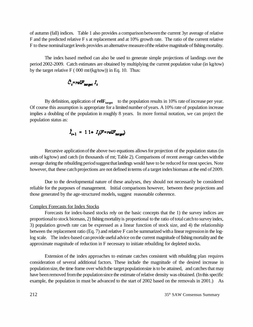
212 35th SAW Consensus Summary
of autumn (fall) indices. Table 1 also provides a comparison between the current 3yr average of relativeF and the predicted relative F s at replacement and at 10% growth rate. The ratio of the current relativeF to these nominal target levels provides an alternative measure of the relative magnitude of fishing mortality.
The index based method can also be used to generate simple projections of landings over theperiod 2002-2009. Catch estimates are obtained by multiplying the current population value (in kg/tow)by the target relative F ( 000 mt/(kg/tow)) in Eq. 10. Thus:
By definition, application of relFtarget to the population results in 10% rate of increase per year.Of course this assumption is appropriate for a limited number of years. A 10% rate of population increaseimplies a doubling of the population in roughly 8 years. In more formal notation, we can project thepopulation status as:
Recursive application of the above two equations allows for projection of the population status (inunits of kg/tow) and catch (in thousands of mt; Table 2). Comparisons of recent average catches with theaverage during the rebuilding period suggest that landings would have to be reduced for most species. Notehowever, that these catch projections are not defined in terms of a target index biomass at the end of 2009.
Due to the developmental nature of these analyses, they should not necessarily be consideredreliable for the purposes of management. Initial comparisons however, between these projections andthose generated by the age-structured models, suggest reasonable coherence.
Complex Forecasts for Index StocksForecasts for index-based stocks rely on the basic concepts that the 1) the survey indices are
proportional to stock biomass, 2) fishing mortality is proportional to the ratio of total catch to survey index,3) population growth rate can be expressed as a linear function of stock size, and 4) the relationshipbetween the replacement ratio (Eq. 7) and relative F can be summarized with a linear regression in the log-log scale. The index-based can provide useful advice on the current magnitude of fishing mortality and theapproximate magnitude of reduction in F necessary to initiate rebuilding for depleted stocks.
Extension of the index approaches to estimate catches consistent with rebuilding plan requiresconsideration of several additional factors. These include the magnitude of the desired increase inpopulation size, the time frame over which the target population size is to be attained, and catches that mayhave been removed from the population since the estimate of relative density was obtained. (In this specificexample, the population in must be advanced to the start of 2002 based on the removals in 2001.) As
35th SAW Consensus Summary 213
noted earlier, the index methodology is not sufficient to uniquely specify the target level of relative biomass.Instead this information is obtained from examination of the trajectories of one or more survey indices, andexternal information about the historical fisheries. These data are often sufficient to allow scientists todefine a proper target biomass. In most instances the defined target biomass coincides with a period ofmoderate to high abundance, stable catches and replacement ratios at or above 1.0. Let ITARGET(T)represent the desired relative population size at year T, the end year of the rebuilding period. The currentcondition of the resource at the start of the rebuilding period is defined as ICURRENT(t) . In order to growfrom ICURRENT(t) to ITARGET(T) over the period t to T the population must grow at a constant averagerate of at least Qrebuild which is defined as:
The next step is to estimate the relative F necessary to induce a population growth rate equal toQrebuild. The robust linear regression model (Eq. 8 Working Group Report) can be used to estimate therelative F sufficient for rebuilding (relF rebuild). This can be defined by rearranging Eq. 8 (Working GroupReport) to solve for relF rebuild as follows:
The projected catches consistent with the rebuilding strategy can now be estimated by multiplyingthe relative F by the current index of abundance, i.e.,
The last step in the projection process is to project the population to the next year. This isaccomplished by multiplying the current population by the Qrebuild.
The preceding two equations are simply applied recursively until year T, the end of the rebuildingperiod.
A complication that arises for projection of catches in 2002 and 2003 is that neither the catchesnor survey values in 2001 were available when the index-based reference points were derived. The valuesin Tables 1 and 2 represent estimates for year 2000 relative biomasses and relative fishing mortality rates.
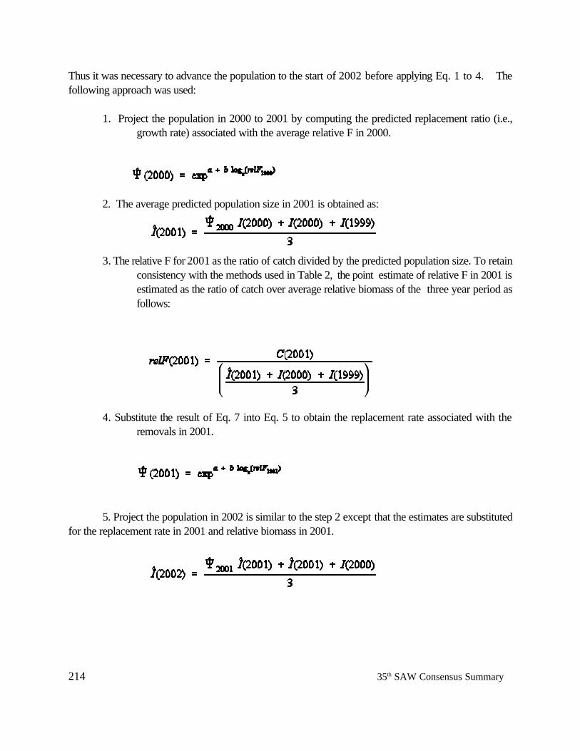
214 35th SAW Consensus Summary
Thus it was necessary to advance the population to the start of 2002 before applying Eq. 1 to 4. Thefollowing approach was used:
1. Project the population in 2000 to 2001 by computing the predicted replacement ratio (i.e.,growth rate) associated with the average relative F in 2000.
2. The average predicted population size in 2001 is obtained as:
3. The relative F for 2001 as the ratio of catch divided by the predicted population size. To retainconsistency with the methods used in Table 2, the point estimate of relative F in 2001 isestimated as the ratio of catch over average relative biomass of the three year period asfollows:
4. Substitute the result of Eq. 7 into Eq. 5 to obtain the replacement rate associated with theremovals in 2001.
5. Project the population in 2002 is similar to the step 2 except that the estimates are substitutedfor the replacement rate in 2001 and relative biomass in 2001.
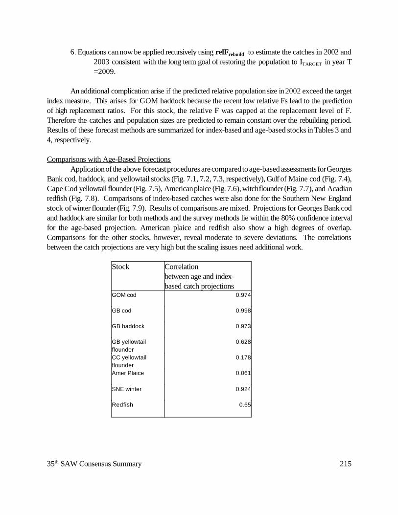
35th SAW Consensus Summary 215
6. Equations can now be applied recursively using relFrebuild to estimate the catches in 2002 and2003 consistent with the long term goal of restoring the population to ITARGET in year T=2009.
An additional complication arise if the predicted relative population size in 2002 exceed the targetindex measure. This arises for GOM haddock because the recent low relative Fs lead to the predictionof high replacement ratios. For this stock, the relative F was capped at the replacement level of F.Therefore the catches and population sizes are predicted to remain constant over the rebuilding period.Results of these forecast methods are summarized for index-based and age-based stocks in Tables 3 and4, respectively.
Comparisons with Age-Based ProjectionsApplication of the above forecast procedures are compared to age-based assessments for Georges
Bank cod, haddock, and yellowtail stocks (Fig. 7.1, 7.2, 7.3, respectively), Gulf of Maine cod (Fig. 7.4),Cape Cod yellowtail flounder (Fig. 7.5), American plaice (Fig. 7.6), witch flounder (Fig. 7.7), and Acadianredfish (Fig. 7.8). Comparisons of index-based catches were also done for the Southern New Englandstock of winter flounder (Fig. 7.9). Results of comparisons are mixed. Projections for Georges Bank codand haddock are similar for both methods and the survey methods lie within the 80% confidence intervalfor the age-based projection. American plaice and redfish also show a high degrees of overlap.Comparisons for the other stocks, however, reveal moderate to severe deviations. The correlationsbetween the catch projections are very high but the scaling issues need additional work.
Stock Correlationbetween age and index-based catch projections
GOM cod 0.974
GB cod 0.998
GB haddock 0.973
GB yellowtailflounder
0.628
CC yellowtailflounder
0.178
Amer Plaice 0.061
SNE winter 0.924
Redfish 0.65
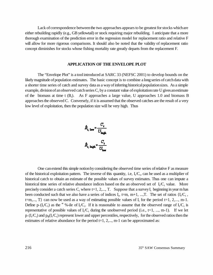
216 35th SAW Consensus Summary
Lack of correspondence between the two approaches appears to be greatest for stocks which areeither rebuilding rapidly (e.g., GB yellowtail) or stock requiring major rebuilding. I anticipate that a morethorough examination of the prediction error in the regression model for replacement ratio and relative Fwill allow for more rigorous comparisons. It should also be noted that the validity of replacement ratioconcept diminishes for stocks whose fishing mortality rate greatly departs from the replacement F.
APPLICATION OF THE ENVELOPE PLOT
The “Envelope Plot” is a tool introduced at SARC 33 (NEFSC 2001) to develop bounds on thelikely magnitude of population estimates. The basic concept is to combine a long series of catch data witha shorter time series of catch and survey data as a way of inferring historical population sizes. As a simpleexample, division of an observed catch series Ct by a constant value of exploitation rate U gives an estimateof the biomass at time t (Bt). As F approaches a large value, U approaches 1.0 and biomass Bapproaches the observed C. Conversely, if it is assumed that the observed catches are the result of a verylow level of exploitation, then the population size will be very high. Thus
One can extend this simple notion by considering the observed time series of relative F as measureof the historical exploitation pattern. The inverse of this quantity, i.e, It/Ct, can be used as a multiplier ofhistorical catch to obtain an estimate of the possible values of survey estimates. Thus one can impute ahistorical time series of relative abundance indices based on the an observed set of It/Ct value. Moreprecisely consider a catch series Ct where t=1, 2,..., T. Suppose that a survey It beginning in year m hasbeen conducted such that we also have a series of indices It, t=m, m+1, ...,T. The set of ratios {It/Ct ,t=m,..., T} can now be used as a way of estimating possible values of It for the period t=1, 2,..., m-1.Define p"(It/Ct) as the "%-ile of It/Ct. If it is reasonable to assume that the observed range of It/Ct isrepresentative of possible values of It/Ct during the unobserved period (i.e., t=1, ..., m-1). If we letp"(It/Ct) and p$(It/Ct) represent lower and upper percentiles, respectively, for the observed ratios then theestimates of relative abundance for the period t=1, 2,..., m-1 can be approximated as:
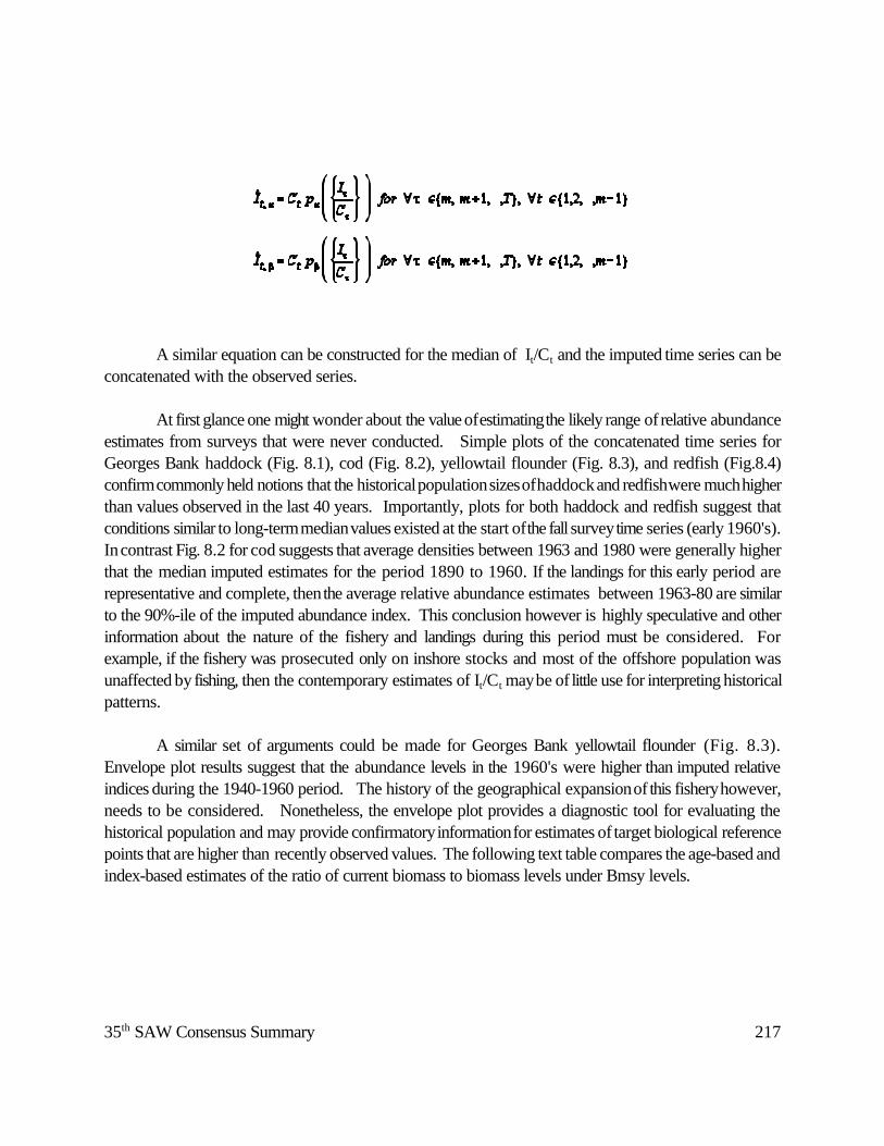
35th SAW Consensus Summary 217
A similar equation can be constructed for the median of It/Ct and the imputed time series can beconcatenated with the observed series.
At first glance one might wonder about the value of estimating the likely range of relative abundanceestimates from surveys that were never conducted. Simple plots of the concatenated time series forGeorges Bank haddock (Fig. 8.1), cod (Fig. 8.2), yellowtail flounder (Fig. 8.3), and redfish (Fig.8.4)confirm commonly held notions that the historical population sizes of haddock and redfish were much higherthan values observed in the last 40 years. Importantly, plots for both haddock and redfish suggest thatconditions similar to long-term median values existed at the start of the fall survey time series (early 1960's).In contrast Fig. 8.2 for cod suggests that average densities between 1963 and 1980 were generally higherthat the median imputed estimates for the period 1890 to 1960. If the landings for this early period arerepresentative and complete, then the average relative abundance estimates between 1963-80 are similarto the 90%-ile of the imputed abundance index. This conclusion however is highly speculative and otherinformation about the nature of the fishery and landings during this period must be considered. Forexample, if the fishery was prosecuted only on inshore stocks and most of the offshore population wasunaffected by fishing, then the contemporary estimates of It/Ct may be of little use for interpreting historicalpatterns.
A similar set of arguments could be made for Georges Bank yellowtail flounder (Fig. 8.3).Envelope plot results suggest that the abundance levels in the 1960's were higher than imputed relativeindices during the 1940-1960 period. The history of the geographical expansion of this fishery however,needs to be considered. Nonetheless, the envelope plot provides a diagnostic tool for evaluating thehistorical population and may provide confirmatory information for estimates of target biological referencepoints that are higher than recently observed values. The following text table compares the age-based andindex-based estimates of the ratio of current biomass to biomass levels under Bmsy levels.
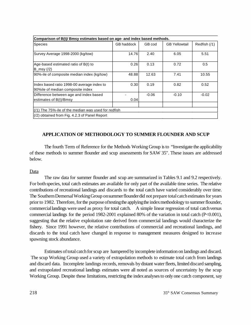
218 35th SAW Consensus Summary
Comparison of B(t)/ Bmsy estimates based on age- and index based methods.Species GB haddock GB cod GB Yellowtail Redfish (/1)
Survey Average 1998-2000 (kg/tow) 14.76 2.40 6.05 5.51
Age-based estimated ratio of B(t) to B_msy (/2)
0.26 0.13 0.72 0.5
90%-ile of composite median index (kg/tow) 48.88 12.63 7.41 10.55
Index based ratio 1998-00 average index to90%ile of median composite index
0.30 0.19 0.82 0.52
Difference between age and index basedestimates of B(t)/Bmsy
-0.04
-0.06 -0.10 -0.02
(/1) The 75%-ile of the median was used for redfish (/2) obtained from Fig. 4.2.3 of Panel Report
APPLICATION OF METHODOLOGY TO SUMMER FLOUNDER AND SCUP
The fourth Term of Reference for the Methods Working Group is to “Investigate the applicabilityof these methods to summer flounder and scup assessments for SAW 35". These issues are addressedbelow.
DataThe raw data for summer flounder and scup are summarized in Tables 9.1 and 9.2 respectively.
For both species, total catch estimates are available for only part of the available time series. The relativecontributions of recreational landings and discards to the total catch have varied considerably over time.The Southern Demersal Working Group on summer flounder did not prepare total catch estimates for yearsprior to 1982. Therefore, for the purpose of testing the applying the index methodology to summer flounder,commercial landings were used as proxy for total catch. A simple linear regression of total catch versuscommercial landings for the period 1982-2001 explained 80% of the variation in total catch (P<0.001),suggesting that the relative exploitation rate derived from commercial landings would characterize thefishery. Since 1991 however, the relative contributions of commercial and recreational landings, anddiscards to the total catch have changed in response to management measures designed to increasespawning stock abundance.
Estimates of total catch for scup are hampered by incomplete information on landings and discard. The scup Working Group used a variety of extrapolation methods to estimate total catch from landingsand discard data. Incomplete landings records, removals by distant water fleets, limited discard sampling,and extrapolated recreational landings estimates were all noted as sources of uncertainty by the scupWorking Group. Despite these limitations, restricting the index analyses to only one catch component, say
35th SAW Consensus Summary 219
Summer FlounderFall Survey Spring SurveyRandomization Test Summary Randomization Test Summary Observed Correlation -0.622 Observed Correlation -0.619
Sampling Distribution Stats Sampling Distribution Statsmedian -0.308 median -0.317
min -0.664 min -0.744max 0.239 max 0.273
95%ile -0.015 95%ile -0.0205%ile -0.535 5%ile -0.554
Approximate Significance Approximate SignificanceLevel of test statistic Level of test statistic
P(Corr<Obs Correlation) P(Corr<Obs Correlation)0.00704 0.01829
commercial landings, was considered inappropriate. Therefore the index-based estimates of relative F andreplacement ratios were based on the best estimates of total catch.
Replacement Ratio EstimatesGraphical analyses of summer flounder (Fig. 9.2 , 9.3) reveal similar patterns with respect to the
spring and fall trawl surveys. Both surveys show a strong upward trend in abundance since 1990,consistent with the imposition of quota regulations in same period. Relative F estimates exhibit the oppositetrend and reached the lowest levels on record in 2001. The replacement ratio has increased above 1.0 inthe spring survey (Fig. 9.2) about 1993 and about 1996 in the fall survey (Fig. 9.3). Estimates of therelationship between the replacement ratio and relative F suggest a consistent pattern for both surveys. Asshown below, randomization tests of both regressions were statistically significant. Low levels of relativeF in recent years are strongly associated with replacement ratios above 1.0. The results provide strongevidence that the reduced fishing mortality rates of the past decade have been instrumental in the recovery
of summer flounder.
Results for scup were less conclusive(Fig. 9.3-4). Analyses of the fall survey (Fig. 9.3) suggest thatthe recent increase in fallu survey biomass is strongly associated with the decline in relative F. Thereplacement ratio first increased above 1.0 about 1996 and the regression between replacement ratio andrelative F is statistically significant (below).
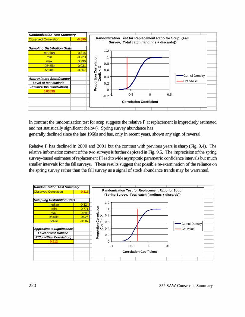
220 35th SAW Consensus Summary
Randomization Test Summary Observed Correlation -0.590
Sampling Distribution Statsmedian -0.314
min -0.723max 0.296
95%ile -0.0315%ile -0.567
Approximate SignificanceLevel of test statistic
P(Corr<Obs Correlation)0.03599
Randomization Test for Replacement Ratio for Scup: {Fall Survey, Total catch (landings + discards)}
-0.2
0
0.2
0.4
0.6
0.8
1
1.2
-1 -0.5 0 0.5
Correlation Coefficient
Prop
ortio
n C
orre
latio
n C
oeff.
< X
Cumul DensityCrit value
Randomization Test Summary Observed Correlation -0.315
Sampling Distribution Statsmedian -0.324
min -0.771max 0.298
95%ile -0.0255%ile -0.587
Approximate SignificanceLevel of test statistic
P(Corr<Obs Correlation)0.512
Randomization Test for Replacement Ratio for Scup: {Spring Survey, Total catch (landings + discards)}
0
0.2
0.4
0.6
0.8
1
1.2
-1 -0.5 0 0.5
Correlation Coefficient
Prop
ortio
n C
orre
latio
n C
oeff.
< X
Cumul DensityCrit value
In contrast the randomization test for scup suggests the relative F at replacement is imprecisely estimatedand not statistically significant (below). Spring survey abundance has generally declined since the late 1960s and has, only in recent years, shown any sign of reversal.
Relative F has declined in 2000 and 2001 but the contrast with previous years is sharp (Fig. 9.4). Therelative information content of the two surveys is further depicted in Fig. 9.5. The imprecision of the springsurvey-based estimates of replacement F lead to wide asymptotic parametric confidence intervals but muchsmaller intervals for the fall surveys. These results suggest that possible re-examination of the reliance onthe spring survey rather than the fall survey as a signal of stock abundance trends may be warranted.
35th SAW Consensus Summary 221
Projections of relative biomass and landingsAs described in Section 7.0 the index methodology can be extended to provide projections of
catch (or landings) and relative stock. The validity of these projections is primarily governed by thedifference in magnitude of the current relative F and the relative F at replacement. As with any linearregression, projections that rely independent variables that are far from their means are less reliable thatestimates close to the mean. For the index methodology, transient effects during stock rebuilding may resultin overly optimistic projections of stock recovery and/or landings.
The projection scenarios for summer flounder and scup (Table 7) were based on a continuationof contemporary rates of relative exploitation. Relative F levels for both summer flounder and scup aresufficiently low such that continuing increases are expected in the short term. Projections for summerflounder suggest a near 3-fold increase in relative biomass and landings through 2005. Projected landingsfor scup are similarly optimistic irrespective of whether the analyses include or exclude discard estimatesfrom the total catch estimates.
The dynamics of both species are likely to be dominated by strong year classes and the projectionsmay not be realistic in the longer term. However, both scenarios suggest that the populations and landingsshould continue to increase in the short run, predictions that are consistent with more detailed projectionsderived from analytical models.
222 35th SAW Consensus Summary
SARC COMMENTS - INDEX METHODS
The SARC reviewed a working document on the development of empirical methods for stockassessments based on analysis of total catch and trends in abundance indices. The work discussed is inprogress and, while it was developed with feedback from the SAW methods group, it had not been subjectto extensive peer review prior to the SARC.
TERMS OF REFERENCE
1. Describe the underlying theoretical basis for the index-based assessment and projectionmethodologies2. Identify critical limitations for application of such methodologies. 3. Compare reference point estimates and projections with results from VPA and other modelingapproaches.4. Investigate the applicability of these methods to summer flounder and scup assessments for SAW35.
Potential of the methodsThe SARC concluded that the method has considerable potential as a monitoring tool that to
evaluate stock trajectories and provide valuable information in interim years between analyticalassessments. Similarly, the technique has utility in presenting an integrated picture of stock dynamics forresources where only catch statistics and survey trends are available. The visual techniques wereconsidered very useful as a summary of stock status trends.
The SARC also discussed the value of the method in terms of its usefulness for providing objectiveestimates of proxies for management reference points. While the method does not provide, a priori, aproxy for Fmsy, it has potential for estimating a relative F for stock replacement, especially in cases wheredensity-dependence is not apparent and other conditions of the method (discussed below) are met. In suchcases, the method may be preferable to subjective methods currently used to provide reference points.Under conditions of low stock density, the level of recruitment is likely to be proportional to stockabundance and thus increase the applicability of the method.
The SARC further provided technical comments on aspects of the derivation of the method, andconditions under which it might be inappropriate to apply this method. Most of these limitations also applyto the application of alternative methods.
Theoretical bases for the methodsA number of issues were raised at the SARC regarding the theoretical basis for the index-based
assessment and projection methods:
35th SAW Consensus Summary 223
! The use of the moving average in the denominator of the replacement ratio statistic could be
generalized to a broader family of smoothing equations, thereby retaining the empirical nature andextending the flexibility of the method; the link to survival and recruitment is an unnecessaryconstraint and may limit the development of better predictors of stock status based on availableindices. On the other hand, development of a theoretical basis for the method could allowinterpretation of underlying assumptions leading to stock replacement.
! The ratio of current biomass to the weighted sum of previous biomasses, as specified in the currentderivation (equation 6) equals one, irrespective of the trend in the population. However, the SARCconcluded that the statistic proposed, defined as the ratio between the last index of abundance andthe moving average of the previous five indices, can be used as an empirical measure of biomasstrend because of variation in population processes (survival and recruitment).
! The basis for estimating the relative rate of fishing mortality at which the stock would replace itselffrom the empirical regression between the index of trend and the relative fishing mortality wasquestioned on the following grounds: if density-dependence was operating, there would be infinitelevels of replacement F; results of the regression approach would reflect a composite of alternativestable points and transient effects. It is possible that clustering of data points in various quadrantscan be taken as indications of multiple stable equilibria.
Conditions for application of the methods
! The method requires the use of reliable catch statistics so it would not be applicable to stocks forwhich catch records are inadequate, or substantial portions of the catch are poorly estimated (e.g.discards, recreational catch etc).
! The method assumes that the survey indices adequately represent the fishable biomass. Concernwas raised by the SARC that this assumption could be problematic as the surveys often catchesyounger fish than the fishery. The problem may be more severe when there have been majorchanges in the exploitation pattern.
! The method will not adequately estimate relF at replacement when stock trends are mainly drivenby environmental effects. Strong year classes or, worse, persistent changes in productivity such asconnected to regime shifts would lead to spurious results.
! The method would be unsuitable for developing fisheries, or situations when fishing mortality isincreasing from a low value. It may be unsuitable for other types of fisheries depending on theirexploitation history, but that needs to be investigated.
224 35th SAW Consensus Summary
! Similar to the limitations of using biomass-weighted F as an overfishing definition (SAW 33) relFand relF rep will be sensitive to transition effects due to variations in recruitment, PR, averageweights, age structure and other factors.
! The validity of the envelope plots used to reconstruct historical stock trajectories clearly dependson the historical exploitation being in the range of observed relFs. In instances where the catchseries represents a developing fishery, then the envelope would be insufficient to estimate stocksize.
Comparison of projections with results from VPA and other modeling approaches
! Projections are based on linear rates of increase and as such they should not be used to projectpopulation trends beyond a few years.
! Projections are sensitive to transient effects even in the absence of density dependence. Forexample, initial stock increases obtained in response to reductions in F may be fast initially but theincrease would slow down as the age structure broadens.
! The selection of the relative F needed to achieve a given rate of increase in the projections wouldbe sensitive to transient conditions. For example, a stock that is rebuilding fast in response to arecent large reduction in F may transiently show a replacement index higher than required; in thiscase the procedure would produce an increase in relative F when in fact such an increase wouldnot be guaranteed. When required relative F differs markedly from the current, catch projectionswill be off scale compared to projections made using conventional age-structured models (e.g. inGB yellowtail).
! Further evaluation of the degree to which the method produces results that are comparable withthose produced by VPA are required, noting that the new method has the potential to be appliedwhen data limit the applicability of other methods
Applicability to summer flounder and scup assessments for SAW 35Due to inadequate catch records, the SARC concluded that the method was not applicable to the
scup assessment.
The method could have potential for summer flounder as an interim technique between analyticalassessments to evaluate new catch and survey data relative to management targets, especially incombination with medium-term projections from assessments.
35th SAW Consensus Summary 225
RESEARCH RECOMMENDATIONS
! Evaluate the performance of the proposed index methods using age-structured simulationsrepresenting different histories of exploitation, fishery selectivity, assumptions of densitydependence, stock trajectories, and time lags.
! Compare reference points resulting from the method with traditional BRPs
ACKNOWLEDGEMENTS
I wish to thank the members of the Working Group on the Re-Evaluation of Biological ReferencePoints for New England Groundfish for their comments and encouragement toward the development of theindex-based methods. I also wish to thank my colleagues in the Population Dynamics Branch for theirassistance and for providing the catch and survey data that comprise the basis of this report. Althoughthere was insufficient time to convene a meeting of the Methods Subcommittee prior to the SARC manyindividual commented on the general approaches described herein. I thank everyone for their contributions.Any errors that remain are mine.
REFERENCES
Applegate, A., S. Cadrin, J. Hoenig, C. Moore, S. Murawski and E. Pikitch. 1998. Evaluation of existingoverfishing definitions and recommendations for new overfishing definitions to comply with theSustainable Fisheries Act. Final Report, Overfishing Definition Review Panel. New EnglandFishery management Council, Newburyport, Massachusetts. 179 pp.
Beverton, R. J. H., and S. J. Holt. 1957. On the dynamics of exploited fish populations. Chapman andHall, London, Fascimile reprint 1993.
Brodziak, J., P. Rago, and R. Conser. 1998. A general approach for making short-term stochasticprojections from an age-structured fisheries assessment model. In F. Funk, T. Quinn II, J. Heifetz,J. Ianelli, J. Powers, J. Schweigert, P. Sullivan, and C.-I. Zhang (Eds.), Proceedings of theInternational Symposium on Fishery Stock Assessment Models for the 21st Century. AlaskaSea Grant College Program, Univ. of Alaska, Fairbanks.
Brodziak, J.T.K, W.J. Overholtz, and P.J. Rago. 2001. Does spawning stock affect recruitment of NewEngland groundfish? Canadian Journal of Fisheries and Aquatic Sciences 58(2):306-318.
Brodziak, J. K. T., and P. J. Rago. 2002. AGEPRO Version 2.0 User’s Guide. Northeast FisheriesScience Center, 166 Water Street, Woods Hole, Massachusetts, 02543, 108 pp.
226 35th SAW Consensus Summary
Brown, B. E., J. A. Brennan, M. D. Grosslein, E. G. Heyerdahl, and R. C. Hennemuth. 1976. The effectof fishing on the marine finfish biomass in the northwest Atlantic from the Gulf of Maine to CapeHatteras. ICNAF Research Bulletin. 12: 49-68.
Burnham, K.P., and Anderson, D.A. 1998. Model selection and inference: A practical informationtheoretic approach. Springer-Verlag, New York.
Carlin, B. P., and T. A. Louis. 2000. Bayes and empirical Bayes methods for data analysis. Chapman andHall, New York.
Clark, C. W. 1976. Mathematical bioeconomics: the optimal management of renewable resources. Wiley-Interscience. New York
Cleveland. W. S. 1993. Visualizing data. Hobart Press. Summit, New Jersey.
Collie, J. S. and M. P. Sissenwine. 1983.Estimating population size from relative abundance data measuredwith error. Can. J. Fish. Aquat. Sci. 40:1871-1879.
Eberhardt, L. L. 196xx. Correlation, regression, and density dependence. Ecology 51:306-310.
Goodall, C. 1983. M-Estimators of Location: An outline of the theory. pp. 339-403. in D. C.Hoaglin, F. Mosteller and J. W. Tukey eds. Understanding robust and exploratory data analysis. Wiley.
New York. NY.
Hilborn, R. and C.J. Walters. 1992. Quantitative Fisheries Stock Assessment. Chapman and Hall, NewYork.
Kenney, B. C. 1982. Beware of spurious self-correlation. 1041-1048.
Mace, P. M. 1994. Relationships between common biological reference points used as thresholds andtargets of fisheries management strategies. Canadian Journal of Fisheries and Aquatic Sciences51:110-122.
Manly, B. 1997. Randomization, bootstrap, and Monte Carlo methods in biology. 2nd ed. Chapman andHall, New York.
Mosteller, F. and J.W. Tukey. 1977. Data analysis and regression. Addison-Wesley. Reading, MA
NEFSC (Northeast Fisheries Science Center). 2001. Report of the 33rd Northeast Regional StockAssessment Workshop (33rd SAW). Stock Assessment Review Committee (SARC) ConsensusSummary of Assessments. Northeast Fish. Sci. Cent. Ref. Doc. 01-18.
35th SAW Consensus Summary 227
_________. 2002. Appendix 7 to the “Final Report of the Working Group on Re-Evaluation of BiologicalReference Points for New England Groundfish”. Northeast Fish. Sci. Cent. Ref. Doc. 02-04. pp.129-163.
National Research Council (NRC). 1998a. Improving Fish Stock Assessments. National Academy Press,Washington, DC.
National Research Council (NRC). 1998b. Review of Northeast fishery stock assessments. NationalAcademy Press, Washington, DC 128 pp.
Rago, P. J. 2001. Index measures and stock assessment in Atlantic salmon. pp. 137-176 in E. Prevost andG. Chaput.eds. Stock, recruitment and reference points: assessment and management of Atlanticsalmon. INRA Editions. Paris.
Prager, M.H. 1994. A suite of extensions to a nonequilibrium surplus-production model. Fish. Bull. 92:374-389.
Quinn, T. J., II, and R. B. Deriso. 1998. Quantitative fish dynamics. Oxford University Press, Oxford,U.K.
Schnute, J. T. 1985. A general theory for analysis of catch and effort data. Can. J. Fish. Aquat. Sci.42:414-429.
Schnute, J. T., and L. J. Richards. 2001. Use and abuse of fishery models. Can. J. Fish. Aquat. Sci.58:10-17.
Simonoff, J. S. 1996. Smoothing methods in statistics. Springer-Verlag. New York.
Sissenwine, M. P., and J. G. Shepherd. 1987. An alternative perspective on recruitment overfishing andbiological reference points. Can. J. Fish. Aquat. Sci. 44:913-918.
Vaughan, D. S. and S. B. Saila. 1976. A method for determining mortality rates using the Leslie matrixmodel. Trans. Amer. Fish Soc. 105:380-383.
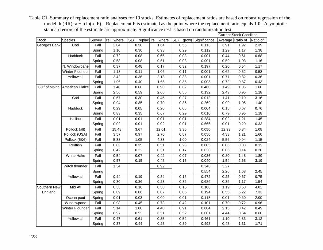
228
Table C1. Summary of replacement ratio analyses for 19 stocks. Estimates of replacement ratios are based on robust regression of themodel ln(RR)=a + b ln(relF). Replacement F is estimated as the point where the replacement ratio equals 1.0. Asymptoticstandard errors of the estimate are approximate. Significance test is based on randomization test.
Current Stock ConditionStock Species Survey relF where SE(F_replac relF where SE (F grow) Significance Average Ratio of Ratio ofGeorges Bank Cod Fall 2.04 0.58 1.64 0.56 0.113 3.91 1.92 2.39
Spring 1.10 0.30 0.93 0.29 0.112 1.29 1.17 1.38Haddock Fall 0.72 0.08 0.65 0.08 0.001 0.44 0.61 0.68
Spring 0.58 0.08 0.51 0.08 0.001 0.59 1.03 1.16N. Windowpane Fall 0.37 0.48 0.17 0.32 0.197 0.20 0.54 1.17Winter Flounder Fall 1.18 0.11 1.06 0.11 0.001 0.62 0.52 0.58
Yellowtail Fall 2.42 0.36 2.13 0.33 0.001 0.77 0.32 0.36Spring 1.96 0.40 1.68 0.36 0.003 0.72 0.37 0.43
Gulf of Maine American Plaice Fall 1.40 0.60 0.90 0.62 0.460 1.49 1.06 1.66Spring 2.56 0.59 2.06 0.55 0.132 2.43 0.95 1.18
Cod Fall 0.67 0.30 0.45 0.27 0.012 1.41 2.10 3.16Spring 0.94 0.35 0.70 0.35 0.269 0.99 1.05 1.40
Haddock Fall 0.23 0.05 0.20 0.05 0.004 0.15 0.67 0.76Spring 0.83 0.35 0.67 0.29 0.010 0.79 0.95 1.18
Halibut Fall 0.01 0.01 0.01 0.01 0.284 0.02 1.21 1.45Spring 0.02 0.01 0.02 0.01 0.665 0.01 0.29 0.33
Pollock (all) Fall 15.48 3.67 12.01 3.36 0.050 12.93 0.84 1.08Pollock (USA) Fall 3.57 0.97 2.70 0.87 0.050 4.33 1.21 1.60Pollock (5&6) Fall 5.88 1.05 4.83 1.00 0.024 5.56 0.94 1.15
Redfish Fall 0.83 0.35 0.51 0.23 0.005 0.06 0.08 0.13Spring 0.42 0.22 0.31 0.17 0.030 0.06 0.14 0.20
White Hake Fall 0.54 0.07 0.42 0.07 0.036 0.80 1.48 1.89Spring 0.57 0.15 0.48 0.15 0.040 1.54 2.68 3.19
Witch flounder Fall 1.34 0.92 0.346 3.27Spring 0.554 2.26 1.68 2.45
Yellowtail Fall 0.44 0.19 0.34 0.18 0.472 0.25 0.57 0.75Spring 0.30 0.36 0.23 0.35 0.686 0.35 1.17 1.54
Southern New Mid Atl Fall 0.33 0.16 0.30 0.15 0.108 1.19 3.60 4.02England Spring 0.09 0.06 0.07 0.05 0.194 0.55 6.22 7.33
Ocean pout Spring 0.01 0.03 0.00 0.01 0.118 0.01 0.60 2.00Windowpane Fall 0.98 0.45 0.73 0.42 0.101 0.70 0.72 0.96
Winter Flounder Fall 5.14 1.00 4.40 0.91 0.004 2.15 0.42 0.49Spring 6.97 0.53 6.51 0.52 0.001 4.44 0.64 0.68
Yellowtail Fall 0.47 0.61 0.35 0.52 0.461 1.10 2.33 3.12Spring 0.37 0.44 0.28 0.39 0.498 0.48 1.31 1.71
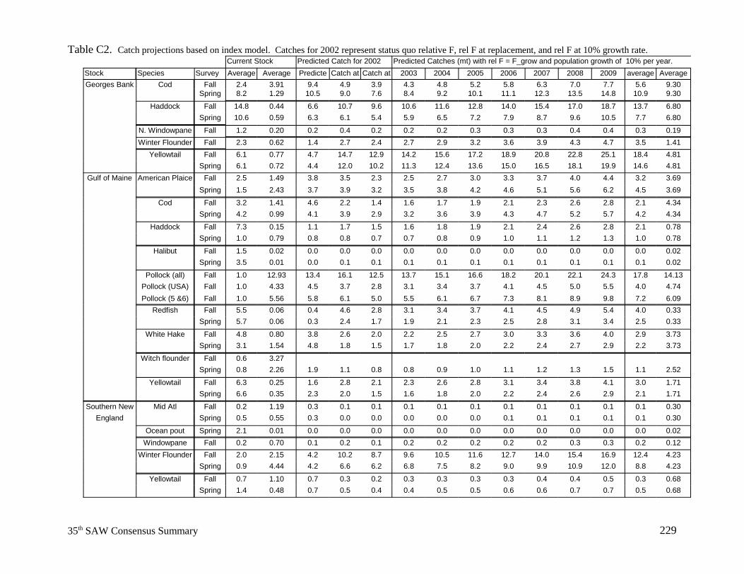
22935th SAW Consensus Summary
Table C2. Catch projections based on index model. Catches for 2002 represent status quo relative F, rel F at replacement, and rel F at 10% growth rate. Current Stock Predicted Catch for 2002 Predicted Catches (mt) with rel F = F_grow and population growth of 10% per year.
Stock Species Survey Average Average Predicte Catch at Catch at 2003 2004 2005 2006 2007 2008 2009 average AverageGeorges Bank Cod Fall 2.4 3.91 9.4 4.9 3.9 4.3 4.8 5.2 5.8 6.3 7.0 7.7 5.6 9.30
Spring 8.2 1.29 10.5 9.0 7.6 8.4 9.2 10.1 11.1 12.3 13.5 14.8 10.9 9.30Haddock Fall 14.8 0.44 6.6 10.7 9.6 10.6 11.6 12.8 14.0 15.4 17.0 18.7 13.7 6.80
Spring 10.6 0.59 6.3 6.1 5.4 5.9 6.5 7.2 7.9 8.7 9.6 10.5 7.7 6.80N. Windowpane Fall 1.2 0.20 0.2 0.4 0.2 0.2 0.2 0.3 0.3 0.3 0.4 0.4 0.3 0.19Winter Flounder Fall 2.3 0.62 1.4 2.7 2.4 2.7 2.9 3.2 3.6 3.9 4.3 4.7 3.5 1.41
Yellowtail Fall 6.1 0.77 4.7 14.7 12.9 14.2 15.6 17.2 18.9 20.8 22.8 25.1 18.4 4.81Spring 6.1 0.72 4.4 12.0 10.2 11.3 12.4 13.6 15.0 16.5 18.1 19.9 14.6 4.81
Gulf of Maine American Plaice Fall 2.5 1.49 3.8 3.5 2.3 2.5 2.7 3.0 3.3 3.7 4.0 4.4 3.2 3.69Spring 1.5 2.43 3.7 3.9 3.2 3.5 3.8 4.2 4.6 5.1 5.6 6.2 4.5 3.69
Cod Fall 3.2 1.41 4.6 2.2 1.4 1.6 1.7 1.9 2.1 2.3 2.6 2.8 2.1 4.34Spring 4.2 0.99 4.1 3.9 2.9 3.2 3.6 3.9 4.3 4.7 5.2 5.7 4.2 4.34
Haddock Fall 7.3 0.15 1.1 1.7 1.5 1.6 1.8 1.9 2.1 2.4 2.6 2.8 2.1 0.78Spring 1.0 0.79 0.8 0.8 0.7 0.7 0.8 0.9 1.0 1.1 1.2 1.3 1.0 0.78
Halibut Fall 1.5 0.02 0.0 0.0 0.0 0.0 0.0 0.0 0.0 0.0 0.0 0.0 0.0 0.02Spring 3.5 0.01 0.0 0.1 0.1 0.1 0.1 0.1 0.1 0.1 0.1 0.1 0.1 0.02
Pollock (all) Fall 1.0 12.93 13.4 16.1 12.5 13.7 15.1 16.6 18.2 20.1 22.1 24.3 17.8 14.13Pollock (USA) Fall 1.0 4.33 4.5 3.7 2.8 3.1 3.4 3.7 4.1 4.5 5.0 5.5 4.0 4.74Pollock (5 &6) Fall 1.0 5.56 5.8 6.1 5.0 5.5 6.1 6.7 7.3 8.1 8.9 9.8 7.2 6.09
Redfish Fall 5.5 0.06 0.4 4.6 2.8 3.1 3.4 3.7 4.1 4.5 4.9 5.4 4.0 0.33Spring 5.7 0.06 0.3 2.4 1.7 1.9 2.1 2.3 2.5 2.8 3.1 3.4 2.5 0.33
White Hake Fall 4.8 0.80 3.8 2.6 2.0 2.2 2.5 2.7 3.0 3.3 3.6 4.0 2.9 3.73Spring 3.1 1.54 4.8 1.8 1.5 1.7 1.8 2.0 2.2 2.4 2.7 2.9 2.2 3.73
Witch flounder Fall 0.6 3.27Spring 0.8 2.26 1.9 1.1 0.8 0.8 0.9 1.0 1.1 1.2 1.3 1.5 1.1 2.52
Yellowtail Fall 6.3 0.25 1.6 2.8 2.1 2.3 2.6 2.8 3.1 3.4 3.8 4.1 3.0 1.71Spring 6.6 0.35 2.3 2.0 1.5 1.6 1.8 2.0 2.2 2.4 2.6 2.9 2.1 1.71
Southern New Mid Atl Fall 0.2 1.19 0.3 0.1 0.1 0.1 0.1 0.1 0.1 0.1 0.1 0.1 0.1 0.30England Spring 0.5 0.55 0.3 0.0 0.0 0.0 0.0 0.0 0.1 0.1 0.1 0.1 0.1 0.30
Ocean pout Spring 2.1 0.01 0.0 0.0 0.0 0.0 0.0 0.0 0.0 0.0 0.0 0.0 0.0 0.02Windowpane Fall 0.2 0.70 0.1 0.2 0.1 0.2 0.2 0.2 0.2 0.2 0.3 0.3 0.2 0.12
Winter Flounder Fall 2.0 2.15 4.2 10.2 8.7 9.6 10.5 11.6 12.7 14.0 15.4 16.9 12.4 4.23Spring 0.9 4.44 4.2 6.6 6.2 6.8 7.5 8.2 9.0 9.9 10.9 12.0 8.8 4.23
Yellowtail Fall 0.7 1.10 0.7 0.3 0.2 0.3 0.3 0.3 0.3 0.4 0.4 0.5 0.3 0.68Spring 1.4 0.48 0.7 0.5 0.4 0.4 0.5 0.5 0.6 0.6 0.7 0.7 0.5 0.68
230 35the SAW Consensus Summary
Part A
a b 1998 1999 2000
Average Relative F (last 3-
yr)
Projected Relative
Biomass in 2001
(kg/tow)
Observed Landings in 2001 (k
mt)
relF estimate in 2001
Projected Relative Biomass in 2002 (kg/tow)
Georges Winter Flounder Fall 0.150 -0.892 1.57 2.64 2.66 0.616 3.13 2.67 0.95 3.20Bank N. Windowpane Fall -0.121 -0.123 1.66 0.73 1.22 0.202 1.082 0.04 0.04 1.24Gulf of Haddock Fall -1.083 -0.733 2.92 4.91 14.03 0.153 9.57 0.95 0.10 13.73Maine Pollock (Area 5 & 6) Fall 0.857 -0.483 0.76 1.52 0.83 5.556 1.14 4.90 4.21 1.11
White Hake Fall -0.243 -0.393 4.27 3.44 6.72 0.798 4.76 3.56 0.72 5.24Spring -0.301 -0.543 1.09 2.97 3.33 1.536 2.71 3.56 1.19 2.63
Southern S.Windowpane Fall -0.008 -0.331 0.18 0.12 0.28 0.702 0.20 0.11 0.56 0.24New SNE Yellowtail Fl Fall -0.243 -0.324 0.90 0.10 0.99 1.099 0.53 1.03 1.91 0.62England Spring -0.358 -0.358 0.97 1.76 1.44 0.481 1.48 1.03 0.66 1.38
Ocean Pout Spring -0.337 -0.079 1.73 2.56 2.02 0.008 2.26 0.02 0.01 2.21MidAtl Yellowtail Fl Fall -0.959 -0.864 0.09 0.50 0.11 1.188 0.23 0.21 0.74 0.15
Part B
Target Relative Biomass (kg/tow)
Annual Growth
rate necessary to rebuild by 2009
Relative F for
Rebuild 2002 2003 2004 2005 2006 2007 2008 2009Georges Winter Flounder Fall 2.74 0.978 1.183 3.79 3.79 3.79 3.79 3.79 3.79 3.79 3.79
Bank N. Windowpane Fall 0.94 0.962 0.373 0.46 0.46 0.46 0.46 0.46 0.46 0.46 0.46Gulf of Haddock Fall 22.17 1.071 0.208 2.86 3.06 3.28 3.51 3.76 4.02 4.31 4.61Maine Pollock (Area 5 & 6) Fall 3.00 1.153 4.381 4.84 5.58 6.44 7.43 8.57 9.88 11.39 13.14
White Hake Fall 12.00 1.126 0.399 2.09 2.35 2.65 2.98 3.36 3.78 4.25 4.79Spring 12.00 1.242 0.385 1.01 1.26 1.56 1.94 2.41 2.99 3.72 4.62
Southern S.Windowpane Fall 0.92 1.210 0.550 0.13 0.16 0.20 0.24 0.29 0.35 0.42 0.51New SNE Yellowtail Fl Fall 15.00 1.577 0.116 0.07 0.11 0.18 0.28 0.44 0.70 1.10 1.74
England Spring 12.00 1.363 0.155 0.21 0.29 0.40 0.54 0.73 1.00 1.36 1.86Ocean Pout Spring 4.90 1.120 0.003 0.01 0.01 0.01 0.01 0.01 0.01 0.01 0.02
MidAtl Yellowtail Fl Fall 12.91 1.887 0.158 0.02 0.05 0.09 0.16 0.30 0.57 1.08 2.04
Projection of Stock from 2000 to 2002
Predicted Catch (k mt)
Stock Species
Stock Species Survey
Biological Targets
Survey
Parameters ln(RR) =a+b ln(relF) Survey Estimates (kg/tow)
Table C3. Catch projection estimates for index based stocks. Target index values are externally supplied and are based on analysis of the historical fishery and trends in research survey indices. PartA illustrates the initial projection from 2000 to 2002 based on the observed landings in 2001 and methodology described in the text. Part B summarizes the catch projections given the annual growthrates necessary to reach the biomass targets in 2009.
23135th SAW Consensus Summary
Part A
a b 1998 1999 2000
Average Relative F (last 3-
yr)
Projected Relative Biomass in 2001 (kg/tow)
Observed Landings in 2001 (k
mt)
relF estimate in 2001
Projected Relative
Biomass in 2002
(kg/tow)Cod Fall 0.310 -0.436 2.80 3.00 1.40 3.911 2.07 12.77 5.92 1.59 3.88
Spring 0.053 -0.574 11.70 4.70 8.20 1.285 6.79 12.77 1.94 6.63 3.88Haddock Fall -0.281 -0.873 5.75 23.13 15.41 0.445 20.38 11.55 0.59 20.08 2.70
Spring -0.433 -0.785 6.12 7.75 17.88 0.592 11.99 11.55 0.92 12.72 2.70Yellowtail Fl. Fall 0.651 -0.735 4.35 7.97 5.84 0.769 9.29 7.74 1.00 10.96 1.30
Spring 0.406 -0.601 2.32 9.31 6.70 0.723 9.05 7.74 0.93 9.98 1.30Cod Fall -0.092 -0.233 1.50 3.50 4.70 1.413 3.64 7.99 2.03 3.72 4.05
Spring -0.019 -0.325 4.20 5.10 3.20 0.990 4.13 7.99 1.93 3.54 4.05Redfish Fall -0.036 -0.193 6.49 4.68 5.36 0.064 6.36 0.33 0.06 7.43 1.19
Spring -0.252 -0.293 1.60 3.89 11.46 0.060 8.45 0.33 0.04 12.20 1.19Witch flounder Fall 0.075 -0.254 0.47 0.88 1.11 2.259 0.90 3.46 3.59 0.91 0.81
C.C. Yellowtail Fl. Fall -0.280 -0.344 2.53 9.28 7.12 0.253 8.02 2.57 0.32 8.05 6.10Spring -0.410 -0.340 1.81 2.85 15.15 0.350 8.09 2.57 0.30 10.46 6.10
American Plaice Fall 0.072 -0.214 2.22 2.57 2.80 1.488 2.62 5.37 2.02 2.62 1.89Spring 0.416 -0.444 1.11 1.20 2.30 2.427 1.69 5.37 3.10 1.85 1.89
Winter Flounder Fall 0.998 -0.610 2.23 1.55 2.14 2.148 2.35 4.75 2.36 2.76 1.65Spring 2.701 -1.391 0.85 1.25 1.12 4.439 1.38 4.75 3.80 1.91 1.65
Part B
Target Relative Biomass (kg/tow)
Annual Growth
rate necessary to rebuild by 2009
Relative F for Rebuild 2002 2003 2004 2005 2006 2007 2008 2009
Cod Fall 6.17 1.214 1.306 2.08 2.50 3.10 3.70 4.50 5.50 6.60 8.10Spring 25.74 1.214 0.782 5.18 6.29 7.64 9.27 11.25 13.66 16.58 20.13
Haddock Fall 54.17 1.152 0.616 12.37 14.25 16.43 18.93 21.81 25.13 28.96 33.38Spring 34.33 1.152 0.481 6.12 7.06 8.13 9.37 10.80 12.44 14.34 16.52
Yellowtail Fl. Fall 14.30 1.039 2.302 25.23 26.21 27.22 28.28 29.37 30.51 31.69 32.91Spring 13.02 1.039 1.844 18.41 19.12 19.86 20.63 21.43 22.26 23.12 24.01
Cod Fall 15.08 1.221 0.285 1.06 1.29 1.58 1.93 2.36 2.88 3.52 4.29Spring 14.34 1.221 0.511 1.81 2.21 2.70 3.29 4.02 4.91 6.00 7.33
Redfish Fall 8.87 1.026 0.726 5.39 5.53 5.67 5.82 5.97 6.12 6.28 6.44Spring 14.58 1.026 0.388 4.73 4.86 4.98 5.11 5.24 5.38 5.51 5.66
Witch flounder Fall 0.73 0.970 1.343 1.22 1.22 1.22 1.22 1.22 1.22 1.22 1.22C.C. Yellowtail Fl. Fall 49.13 1.295 0.210 1.69 2.18 2.83 3.66 4.74 6.14 7.95 10.30
Spring 63.80 1.295 0.140 1.46 1.90 2.46 3.18 4.12 5.33 6.90 8.94American Plaice Fall 4.93 1.095 0.916 2.40 2.62 2.87 3.15 3.44 3.77 4.13 4.52
Spring 3.48 1.095 2.084 3.85 4.22 4.61 5.05 5.53 6.06 6.63 7.26Winter Flounder Fall 4.56 1.074 4.574 12.62 13.56 14.57 15.65 16.81 18.06 19.41 20.85
Spring 3.15 1.074 6.621 12.63 13.56 14.57 15.66 16.82 18.07 19.41 20.85
Gulf of Maine
S. New England
Survey
Biological Targets Predicted Catch (k mt)
Georges Bank
Gulf of Maine
S. New England
Stock Species
Survey Estimates (kg/tow) Projection of Stock from 2000 to 2002
Target Increase ratio in mean SSB between 2002 and 2010
Georges Bank
Stock Species Survey
Parameters ln(RR) =a+b ln(relF)
Table C4. Catch projectionestimates for stocks assessed withage structured models. Target indexvalues are derived by multiplyingthe ratio of total biomass estimatesB(2009):B(2002) defined in theAGEPRO projections by theprojected index balue in 2002. PartA illustrates the initial projectionfrom 2000 to 2002 based on theobserved landings in 2001 andmethodology described in the text. The last column represents theprojected increase in between 2002and 2009. Part B summarizes the catch projections given the annualgrowth rates necessary to reach thebiomass targets in 2009.
232 35the SAW Consensus Summary
Table C5. Commercial landings of summer flounder, autumn and spring NMFS research trawl abundance indices, and derived relative F and replacement ratios. Note that 2002 index is preliminary.
Year Landings(000 mt)
NEFSCAutumnSurveyWeight(kg) Per
Tow Index
NEFSCSpringSurveyWeight(kg) Per
Tow Index
Relative Fwrt fall
survey (000mt/(kg/tow))
Replacement index
wrt fallsurvey(5yr)
Relative Fwrt spr
survey (000mt/(kg/tow))
Replacement indexwrt sprsurvey(5yr)
1965 4.61966 6.41967 5.9 1.251968 4.1 1.00 0.16 4.311969 3.0 0.61 0.16 5.24 22.221970 4.0 0.13 0.09 11.94 22.751971 4.2 0.27 0.28 18.99 21.941972 4.2 0.27 0.21 10.73 0.41 12.181973 7.3 0.63 0.54 7.97 1.38 10.94 3.001974 10.2 1.86 1.26 6.18 4.87 9.01 4.921975 11.9 2.48 1.61 6.90 3.92 7.35 3.381976 15.1 0.85 2.00 8.94 0.77 8.49 2.561977 13.6 1.75 1.74 13.58 1.44 7.88 1.551978 13.0 0.40 1.43 12.59 0.26 11.05 1.001979 17.9 0.94 0.35 28.19 0.64 21.03 0.221980 14.2 0.57 0.78 19.05 0.44 22.01 0.551981 9.6 0.72 0.80 13.08 0.80 10.65 0.631982 10.4 0.90 1.11 14.93 1.03 12.79 1.091983 13.4 0.47 0.53 19.91 0.67 19.91 0.591984 17.1 0.65 0.38 25.82 0.90 24.36 0.531985 14.7 0.87 1.20 22.35 1.31 18.34 1.671986 12.2 0.45 0.82 22.85 0.62 15.23 1.021987 12.3 0.28 0.38 43.83 0.42 19.58 0.471988 14.7 0.11 0.68 93.74 0.20 33.89 1.031989 8.1 0.08 0.24 64.14 0.17 20.48 0.351990 4.2 0.19 0.27 28.63 0.53 14.65 0.411991 6.2 0.17 0.35 21.97 0.77 17.29 0.731992 7.5 0.49 0.46 32.27 2.95 17.51 1.201993 5.7 0.04 0.48 19.48 0.19 12.25 1.201994 6.6 0.35 0.46 16.20 1.80 14.12 1.281995 7.0 0.83 0.46 12.84 3.35 13.16 1.141996 5.8 0.45 0.67 7.87 1.20 9.95 1.521997 4.0 0.92 0.61 4.06 2.13 5.87 1.211998 5.08 1.58 0.76 3.66 3.05 6.40 1.421999 4.82 1.66 1.01 2.86 2.01 4.17 1.712000 5.085 1.82 1.7 3.00 1.67 3.13 2.422001 4.916 1.61 2.16 2.87 1.25 2.40 2.272002 2.29 1.83
23335th SAW Consensus Summary
Table C6. Total catch of Scup with discard and recreational landings, autumn and spring NMFS research trawl abundance indices, andderived relative F and replacement ratios.
Year TotalCatch
(k mt)
NEFSCAutumnSurveyWeight(kg) Per
Tow Index
NEFSCSpringSurveyWeight(kg) Per
Tow Index
Relative Fwrt fall
survey (000mt/(kg/tow))
Replacementindex wrt fallsurvey (5yr)
Relative Fwrt spring
survey (000mt/(kg/tow))
Replacementindex wrt
spring survey(5yr)
1963 37.7852 1.211964 29.6681 2.23 21.921965 29.0885 0.62 26.771966 21.2802 0.41 25.641967 15.9281 1.46 19.831968 13.6924 0.54 0.94 6.34 0.461969 9.3341 4.48 0.39 5.34 4.26 10.651970 8.0462 0.22 1.30 4.88 0.15 7.401971 7.7174 0.25 1.57 8.24 0.18 6.141972 8.7627 2.34 0.90 7.47 1.68 7.381973 10.4546 0.93 1.09 7.33 0.59 7.74 1.071974 13.0307 1.01 2.06 7.32 0.61 6.79 1.961975 13.5500 3.40 2.61 3.46 3.58 7.82 1.891976 12.2494 7.35 0.53 2.95 4.63 4.91 0.321977 13.9511 1.71 4.35 4.03 0.57 5.60 3.031978 14.6948 1.32 2.59 12.11 0.46 5.30 1.221979 14.1065 0.61 1.38 14.85 0.21 8.36 0.571980 15.7914 0.92 1.09 10.43 0.32 14.06 0.481981 17.4571 3.01 0.90 10.27 1.26 17.40 0.451982 15.4484 1.17 1.02 10.25 0.77 23.77 0.491983 14.5551 0.34 0.03 15.99 0.24 31.64 0.021984 11.0530 1.22 0.33 6.48 1.01 45.42 0.371985 13.7290 3.56 0.37 6.40 2.67 20.29 0.551986 14.5320 1.66 1.33 8.12 0.89 14.83 2.511987 11.6570 0.15 1.24 18.41 0.09 10.60 2.011988 9.5670 0.09 0.73 53.15 0.06 14.54 1.111989 8.7170 0.30 0.004 21.44 0.22 25.05 0.011990 10.3640 0.83 0.31 19.93 0.72 40.70 0.421991 14.3620 0.43 0.45 18.10 0.71 44.42 0.621992 14.0560 1.12 0.21 26.52 3.11 43.47 0.381993 7.6380 0.04 0.31 18.04 0.07 41.66 0.911994 6.3940 0.11 0.03 18.10 0.20 41.70 0.121995 5.7480 0.91 0.12 13.80 1.80 101.44 0.461996 5.5290 0.23 0.02 8.21 0.44 66.35 0.091997 4.5350 0.88 0.11 7.56 1.83 75.58 0.801998 6.1331 0.69 0.05 5.05 1.59 73.60 0.421999 7.1876 2.07 0.09 2.86 3.67 86.25 1.362000 6.0561 4.79 0.11 2.25 5.01 24.55 1.412001 7.5446 1.2 0.54 2.52 0.69 23.21 7.11
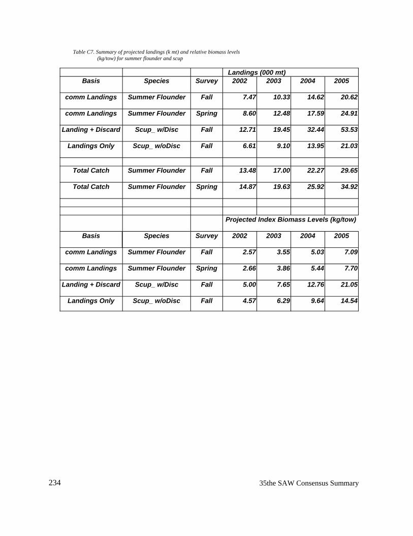
234 35the SAW Consensus Summary
Table C7. Summary of projected landings (k mt) and relative biomass levels (kg/tow) for summer flounder and scup
Landings (000 mt)Basis Species Survey 2002 2003 2004 2005
comm Landings Summer Flounder Fall 7.47 10.33 14.62 20.62
comm Landings Summer Flounder Spring 8.60 12.48 17.59 24.91
Landing + Discard Scup_ w/Disc Fall 12.71 19.45 32.44 53.53
Landings Only Scup_ w/oDisc Fall 6.61 9.10 13.95 21.03
Total Catch Summer Flounder Fall 13.48 17.00 22.27 29.65
Total Catch Summer Flounder Spring 14.87 19.63 25.92 34.92
Projected Index Biomass Levels (kg/tow)
Basis Species Survey 2002 2003 2004 2005
comm Landings Summer Flounder Fall 2.57 3.55 5.03 7.09
comm Landings Summer Flounder Spring 2.66 3.86 5.44 7.70
Landing + Discard Scup_ w/Disc Fall 5.00 7.65 12.76 21.05
Landings Only Scup_ w/oDisc Fall 4.57 6.29 9.64 14.54
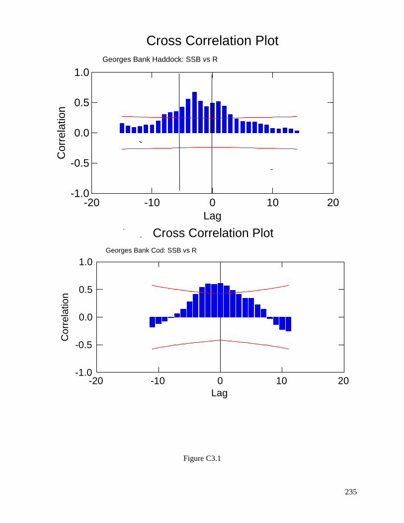
235
Cross Correlation Plot
-20 -10 0 10 20Lag
-1.0
-0.5
0.0
0.5
1.0C
orre
latio
nGeorges Bank Haddock: SSB vs R
Cross Correlation Plot
-20 -10 0 10 20Lag
-1.0
-0.5
0.0
0.5
1.0
Cor
rela
tion
Georges Bank Cod: SSB vs R
Figure C3.1
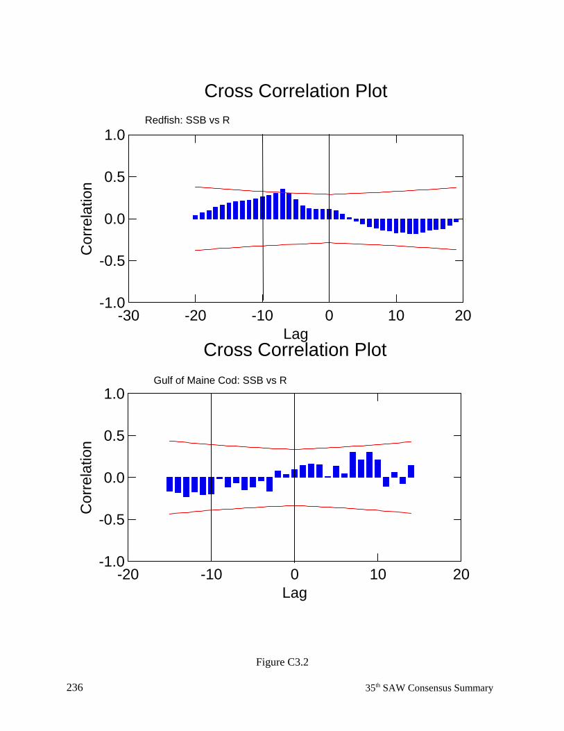
236 35th SAW Consensus Summary
Cross Correlation Plot
-30 -20 -10 0 10 20Lag
-1.0
-0.5
0.0
0.5
1.0
Cor
rela
tion
Redfish: SSB vs R
Cross Correlation Plot
-20 -10 0 10 20Lag
-1.0
-0.5
0.0
0.5
1.0
Cor
rela
tion
Gulf of Maine Cod: SSB vs R
Figure C3.2
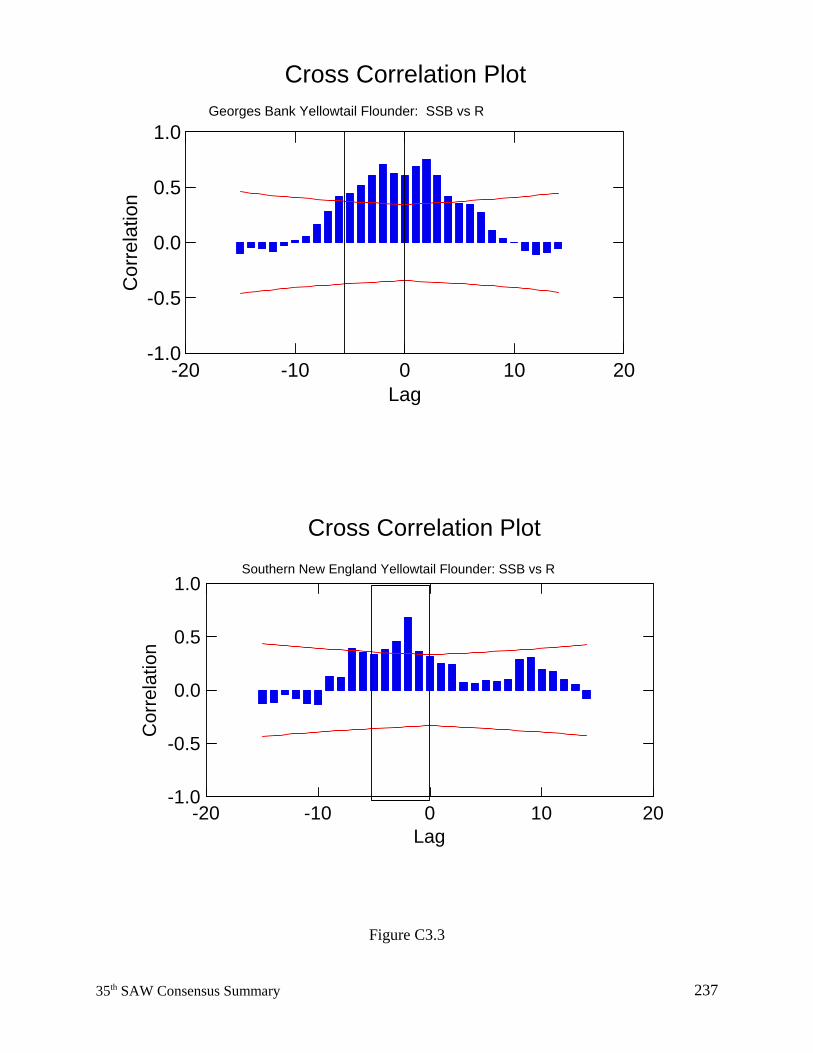
23735th SAW Consensus Summary
Cross Correlation Plot
-20 -10 0 10 20Lag
-1.0
-0.5
0.0
0.5
1.0
Cor
rela
tion
Southern New England Yellowtail Flounder: SSB vs R
Cross Correlation Plot
-20 -10 0 10 20Lag
-1.0
-0.5
0.0
0.5
1.0C
orre
lat io
nGeorges Bank Yellowtail Flounder: SSB vs R
Figure C3.3
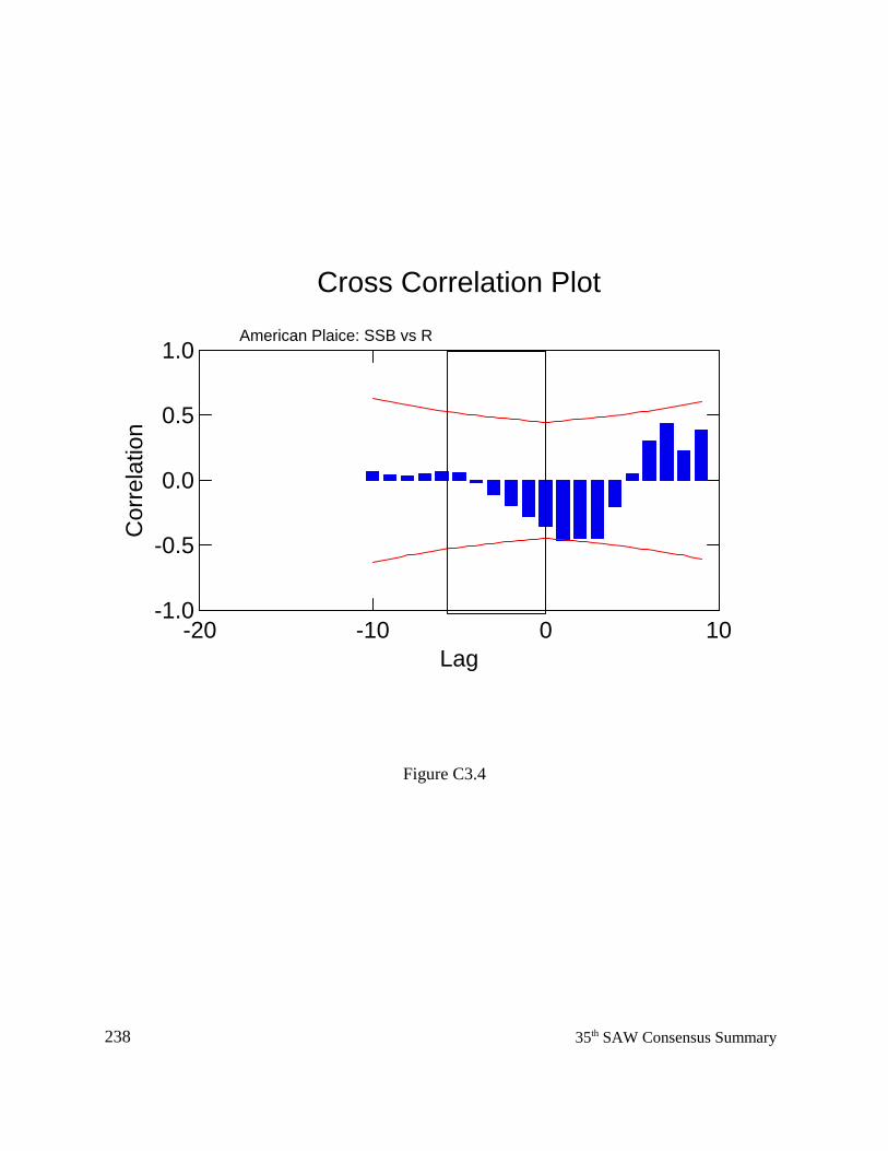
238 35th SAW Consensus Summary
Cross Correlation Plot
-20 -10 0 10Lag
-1.0
-0.5
0.0
0.5
1.0
Cor
rela
tion
American Plaice: SSB vs R
Figure C3.4
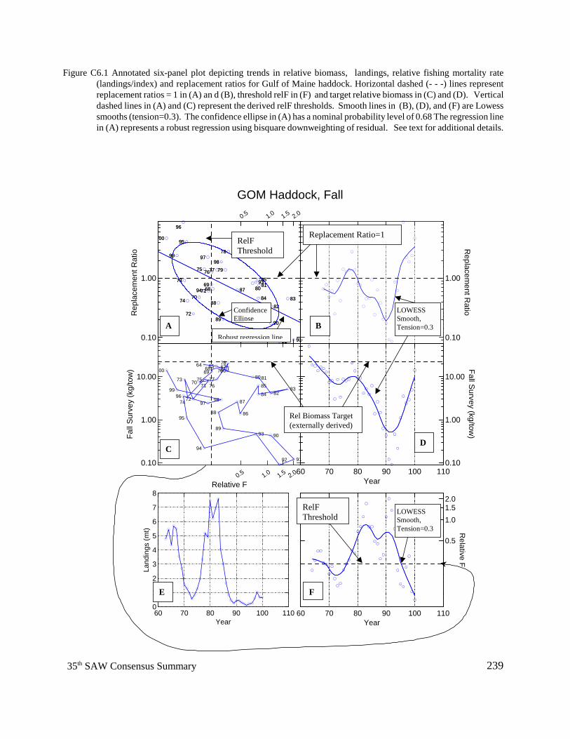
23935th SAW Consensus Summary
GOM Haddock, Fall
0.10
1.00
Rep
lace
men
t Rat
io
00
99
96
73
95
74
72
7094
75
97
7169
76
68
77
91
83
92
82
90
81
84
859380
86
87
78
79
89
98
88
0.5 1.0 1.5 2.0
00
99
96
73
95
74
72
7094
75
97
7169
76
68
77
91
83
92
82
90
81
84
859380
86
87
78
79
89
98
88
0.5 1.0 1.5 2.0
Relative F
0.10
1.00
10.00
Fall
Surv
ey (k
g/to
w) 00
9996
73
95
7472
70
64
94
75
97
71
69
76
6865
77
91
83
92
82
90
81
84
85
93
80
86
87
78676679
89
98
88
60 70 80 90 100 110Year
0
1
2
3
4
5
6
7
8
Land
ings
(mt)
0.10
1.00
Replacem
ent Ratio
60 70 80 90 100 110Year
0.10
1.00
10.00
Fall Survey (kg/tow)
0.5
1.01.52.0
Relative F
60 70 80 90 100 110Year
BA
D C
FE
Replacement Ratio=1 RelF Threshold
RelF Threshold
Rel Biomass Target (externally derived)
Robust regression line
Confidence Ellipse
LOWESS Smooth, Tension=0.3
LOWESS Smooth, Tension=0.3
Figure C6.1 Annotated six-panel plot depicting trends in relative biomass, landings, relative fishing mortality rate(landings/index) and replacement ratios for Gulf of Maine haddock. Horizontal dashed (- - -) lines representreplacement ratios = 1 in (A) an d (B), threshold relF in (F) and target relative biomass in (C) and (D). Verticaldashed lines in (A) and (C) represent the derived relF thresholds. Smooth lines in (B), (D), and (F) are Lowesssmooths (tension=0.3). The confidence ellipse in (A) has a nominal probability level of 0.68 The regression linein (A) represents a robust regression using bisquare downweighting of residual. See text for additional details.
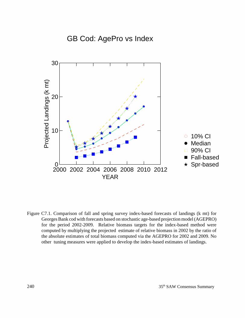
240 35th SAW Consensus Summary
GB Cod: AgePro vs Index
2000 2002 2004 2006 2008 2010 2012YEAR
0
10
20
30
Proj
ecte
d La
n din
gs (k
mt)
Spr-basedFall-based90% CIMedian10% CI
Figure C7.1. Comparison of fall and spring survey index-based forecasts of landings (k mt) forGeorges Bank cod with forecasts based on stochastic age-based projection model (AGEPRO)for the period 2002-2009. Relative biomass targets for the index-based method werecomputed by multiplying the projected estimate of relative biomass in 2002 by the ratio ofthe absolute estimates of total biomass computed via the AGEPRO for 2002 and 2009. Noother tuning measures were applied to develop the index-based estimates of landings.
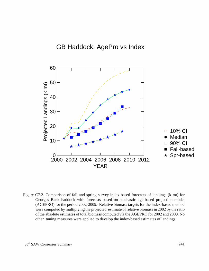
24135th SAW Consensus Summary
GB Haddock: AgePro vs Index
2000 2002 2004 2006 2008 2010 2012YEAR
0
10
20
30
40
50
60
Proj
ecte
d La
ndin
gs (k
mt)
Spr-basedFall-based90% CIMedian10% CI
Figure C7.2. Comparison of fall and spring survey index-based forecasts of landings (k mt) forGeorges Bank haddock with forecasts based on stochastic age-based projection model(AGEPRO) for the period 2002-2009. Relative biomass targets for the index-based methodwere computed by multiplying the projected estimate of relative biomass in 2002 by the ratioof the absolute estimates of total biomass computed via the AGEPRO for 2002 and 2009. Noother tuning measures were applied to develop the index-based estimates of landings.
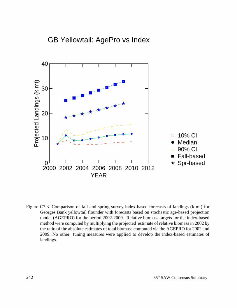
242 35th SAW Consensus Summary
GB Yellowtail: AgePro vs Index
2000 2002 2004 2006 2008 2010 2012YEAR
0
10
20
30
40
Proj
ecte
d La
ndin
gs (k
mt)
Spr-basedFall-based90% CIMedian10% CI
Figure C7.3. Comparison of fall and spring survey index-based forecasts of landings (k mt) forGeorges Bank yellowtail flounder with forecasts based on stochastic age-based projectionmodel (AGEPRO) for the period 2002-2009. Relative biomass targets for the index-basedmethod were computed by multiplying the projected estimate of relative biomass in 2002 bythe ratio of the absolute estimates of total biomass computed via the AGEPRO for 2002 and2009. No other tuning measures were applied to develop the index-based estimates oflandings.
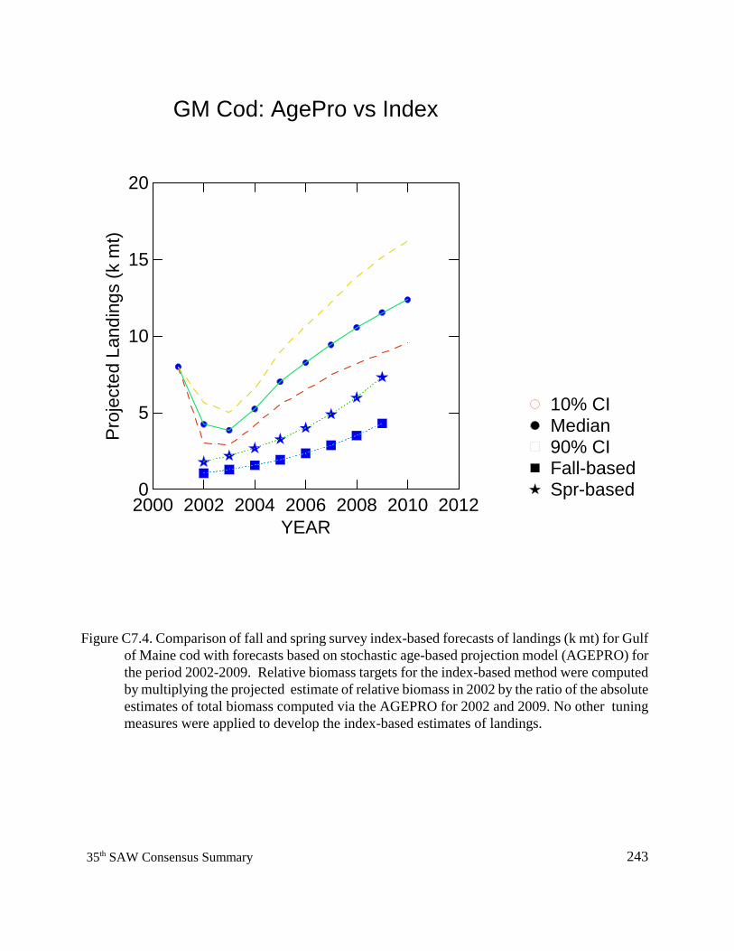
24335th SAW Consensus Summary
GM Cod: AgePro vs Index
2000 2002 2004 2006 2008 2010 2012YEAR
0
5
10
15
20
Proj
ecte
d La
ndin
gs (k
mt)
Spr-basedFall-based90% CIMedian10% CI
Figure C7.4. Comparison of fall and spring survey index-based forecasts of landings (k mt) for Gulfof Maine cod with forecasts based on stochastic age-based projection model (AGEPRO) forthe period 2002-2009. Relative biomass targets for the index-based method were computedby multiplying the projected estimate of relative biomass in 2002 by the ratio of the absoluteestimates of total biomass computed via the AGEPRO for 2002 and 2009. No other tuningmeasures were applied to develop the index-based estimates of landings.
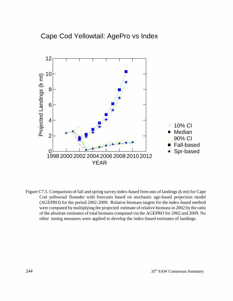
244 35th SAW Consensus Summary
Cape Cod Yellowtail: AgePro vs Index
1998 2000 2002 2004 2006 2008 2010 2012YEAR
0
2
4
6
8
10
12
Proj
ecte
d La
ndin
gs (k
mt)
Spr-basedFall-based90% CIMedian10% CI
Figure C7.5. Comparison of fall and spring survey index-based forecasts of landings (k mt) for CapeCod yellowtail flounder with forecasts based on stochastic age-based projection model(AGEPRO) for the period 2002-2009. Relative biomass targets for the index-based methodwere computed by multiplying the projected estimate of relative biomass in 2002 by the ratioof the absolute estimates of total biomass computed via the AGEPRO for 2002 and 2009. Noother tuning measures were applied to develop the index-based estimates of landings.
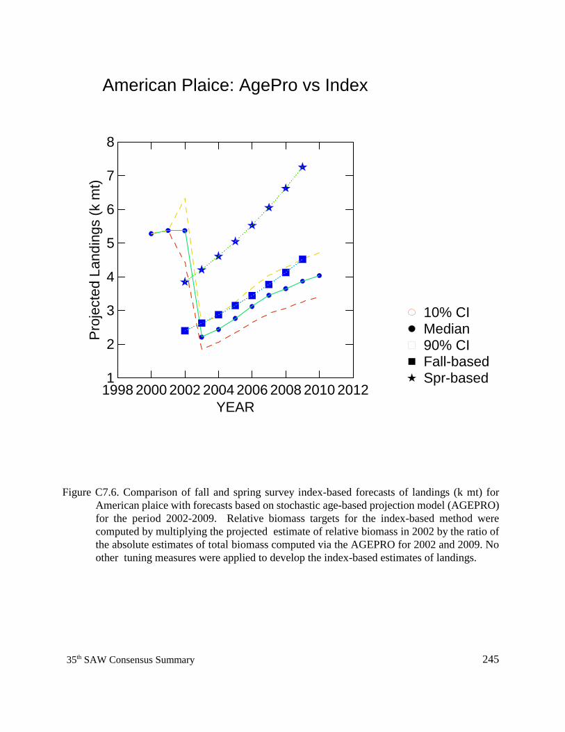
24535th SAW Consensus Summary
American Plaice: AgePro vs Index
1998 2000 2002 2004 2006 2008 2010 2012YEAR
1
2
3
4
5
6
7
8
Proj
ecte
d La
ndin
g s (k
mt)
Spr-basedFall-based90% CIMedian10% CI
Figure C7.6. Comparison of fall and spring survey index-based forecasts of landings (k mt) forAmerican plaice with forecasts based on stochastic age-based projection model (AGEPRO)for the period 2002-2009. Relative biomass targets for the index-based method werecomputed by multiplying the projected estimate of relative biomass in 2002 by the ratio ofthe absolute estimates of total biomass computed via the AGEPRO for 2002 and 2009. Noother tuning measures were applied to develop the index-based estimates of landings.
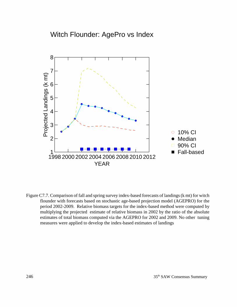
246 35th SAW Consensus Summary
Witch Flounder: AgePro vs Index
1998 2000 2002 2004 2006 2008 2010 2012YEAR
1
2
3
4
5
6
7
8
Proj
ect e
d La
ndin
g s (k
mt)
Fall-based90% CIMedian10% CI
Figure C7.7. Comparison of fall and spring survey index-based forecasts of landings (k mt) for witchflounder with forecasts based on stochastic age-based projection model (AGEPRO) for theperiod 2002-2009. Relative biomass targets for the index-based method were computed bymultiplying the projected estimate of relative biomass in 2002 by the ratio of the absoluteestimates of total biomass computed via the AGEPRO for 2002 and 2009. No other tuningmeasures were applied to develop the index-based estimates of landings
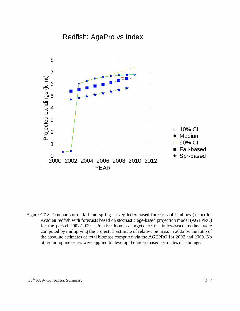
24735th SAW Consensus Summary
Redfish: AgePro vs Index
2000 2002 2004 2006 2008 2010 2012YEAR
0
1
2
3
4
5
6
7
8
Proj
ect e
d La
ndin
g s (k
mt)
Spr-basedFall-based90% CIMedian10% CI
Figure C7.8. Comparison of fall and spring survey index-based forecasts of landings (k mt) forAcadian redfish with forecasts based on stochastic age-based projection model (AGEPRO)for the period 2002-2009. Relative biomass targets for the index-based method werecomputed by multiplying the projected estimate of relative biomass in 2002 by the ratio ofthe absolute estimates of total biomass computed via the AGEPRO for 2002 and 2009. Noother tuning measures were applied to develop the index-based estimates of landings.
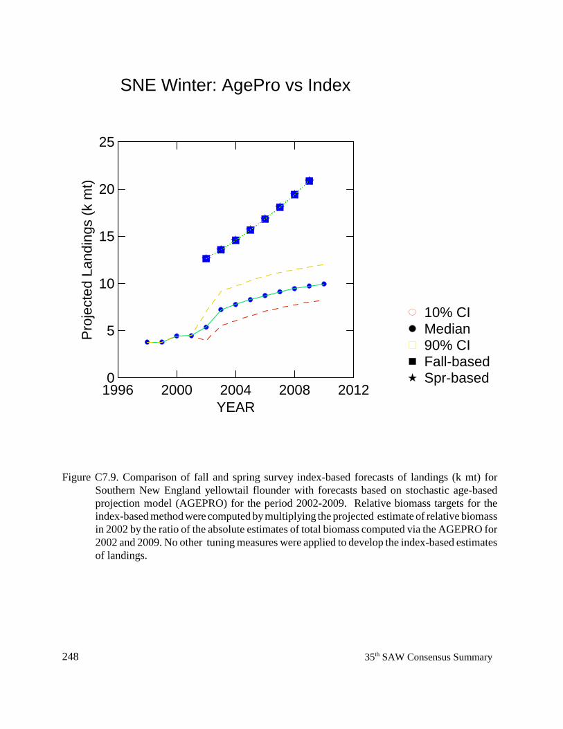
248 35th SAW Consensus Summary
SNE Winter: AgePro vs Index
1996 2000 2004 2008 2012YEAR
0
5
10
15
20
25
Proj
ecte
d La
ndin
g s (k
mt)
Spr-basedFall-based90% CIMedian10% CI
Figure C7.9. Comparison of fall and spring survey index-based forecasts of landings (k mt) forSouthern New England yellowtail flounder with forecasts based on stochastic age-basedprojection model (AGEPRO) for the period 2002-2009. Relative biomass targets for theindex-based method were computed by multiplying the projected estimate of relative biomassin 2002 by the ratio of the absolute estimates of total biomass computed via the AGEPRO for2002 and 2009. No other tuning measures were applied to develop the index-based estimatesof landings.
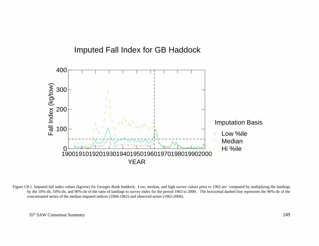
24935th SAW Consensus Summary
Imputed Fall Index for GB Haddock
19001910192019301940195019601970198019902000YEAR
0
100
200
300
400
Fall
Ind e
x (k
g/to
w)
Hi %ileMedianLow %ile
Imputation Basis
Figure C8.1. Imputed fall index values (kg/tow) for Georges Bank haddock. Low, median, and high survey values prior to 1963 are computed by multiplying the landingsby the 10%-ile, 50%-ile, and 90%-ile of the ratio of landings to survey index for the period 1963 to 2000. The horizontal dashed line represents the 90%-ile of theconcatenated series of the median imputed indices (1904-1962) and observed series (1963-2000).
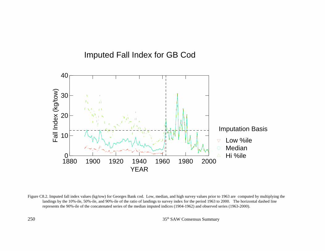
250 35th SAW Consensus Summary
Imputed Fall Index for GB Cod
1880 1900 1920 1940 1960 1980 2000YEAR
0
10
20
30
40
Fall
Inde
x (k
g/to
w)
Hi %ileMedianLow %ile
Imputation Basis
Figure C8.2. Imputed fall index values (kg/tow) for Georges Bank cod. Low, median, and high survey values prior to 1963 are computed by multiplying thelandings by the 10%-ile, 50%-ile, and 90%-ile of the ratio of landings to survey index for the period 1963 to 2000. The horizontal dashed linerepresents the 90%-ile of the concatenated series of the median imputed indices (1904-1962) and observed series (1963-2000).
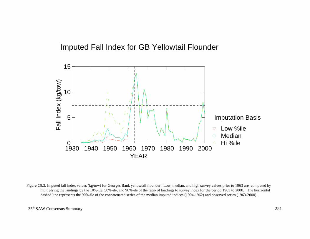
25135th SAW Consensus Summary
Imputed Fall Index for GB Yellowtail Flounder
1930 1940 1950 1960 1970 1980 1990 2000YEAR
0
5
10
15Fa
ll In
dex
(kg/
tow
)
Hi %ileMedianLow %ile
Imputation Basis
Figure C8.3. Imputed fall index values (kg/tow) for Georges Bank yellowtail flounder. Low, median, and high survey values prior to 1963 are computed bymultiplying the landings by the 10%-ile, 50%-ile, and 90%-ile of the ratio of landings to survey index for the period 1963 to 2000. The horizontaldashed line represents the 90%-ile of the concatenated series of the median imputed indices (1904-1962) and observed series (1963-2000).
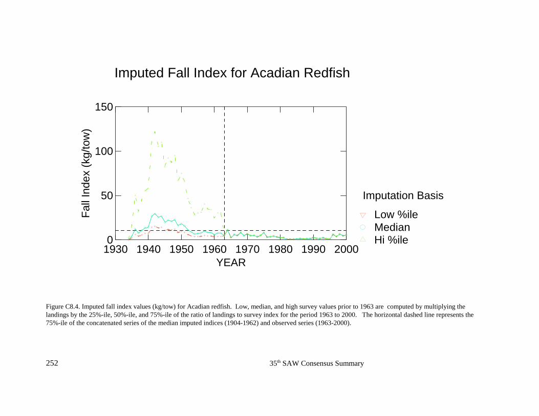
252 35th SAW Consensus Summary
Imputed Fall Index for Acadian Redfish
1930 1940 1950 1960 1970 1980 1990 2000YEAR
0
50
100
150
Fall
Ind e
x (k
g/to
w)
Hi %ileMedianLow %ile
Imputation Basis
Figure C8.4. Imputed fall index values (kg/tow) for Acadian redfish. Low, median, and high survey values prior to 1963 are computed by multiplying thelandings by the 25%-ile, 50%-ile, and 75%-ile of the ratio of landings to survey index for the period 1963 to 2000. The horizontal dashed line represents the75%-ile of the concatenated series of the median imputed indices (1904-1962) and observed series (1963-2000).
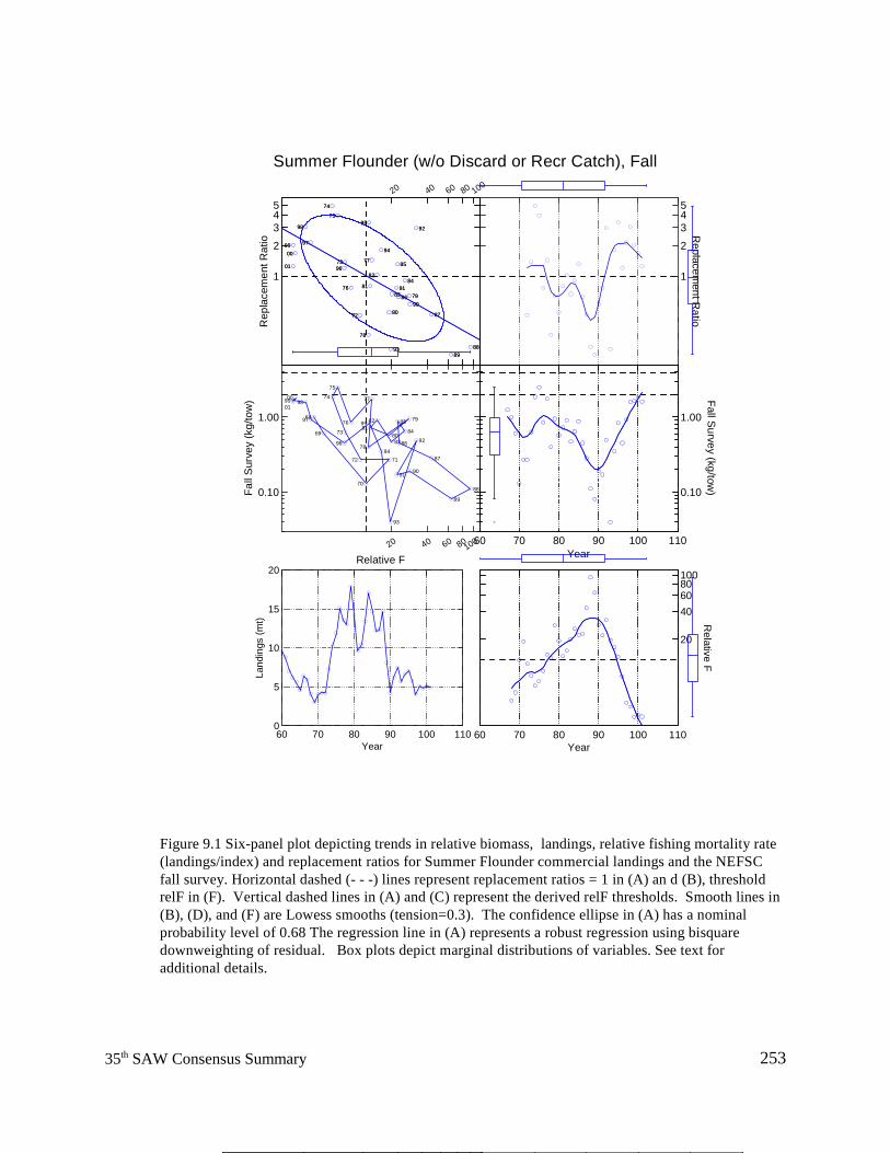
25335th SAW Consensus Summary
g
Summer Flounder (w/o Discard or Recr Catch), Fall
1
2345
Rep
lace
men
t Rat
io 99
01
8889
87
92
9079
84
86
85
9183
93
80
94
82
77
81
95
78
72
76
7396
75
74
97
98
00
20 40 60 80 100
99
01
8889
87
92
9079
84
86
85
9183
93
80
94
82
77
81
95
78
72
76
7396
75
74
97
98
00
20 40 60 80100
Relative F
0.10
1.00
Fall
Sur
vey
(kg/
tow
) 9901
88
89
87
92
90
79
84
86
85
91
83
93
80
7194
82
77
8195
78
70
72
76
73
96
75
74
69
6897
9800
60 70 80 90 100 110Year
0
5
10
15
20
Land
ings
(mt)
1
2345
Replacem
ent Ratio
60 70 80 90 100 110Year
0.10
1.00
Fall Survey (kg/tow)
20
406080100
Relative F
60 70 80 90 100 110Year
Figure 9.1 Six-panel plot depicting trends in relative biomass, landings, relative fishing mortality rate (landings/index) and replacement ratios for Summer Flounder commercial landings and the NEFSC fall survey. Horizontal dashed (- - -) lines represent replacement ratios = 1 in (A) an d (B), threshold relF in (F). Vertical dashed lines in (A) and (C) represent the derived relF thresholds. Smooth lines in (B), (D), and (F) are Lowess smooths (tension=0.3). The confidence ellipse in (A) has a nominal probability level of 0.68 The regression line in (A) represents a robust regression using bisquaredownweighting of residual. Box plots depict marginal distributions of variables. See text for additional details.
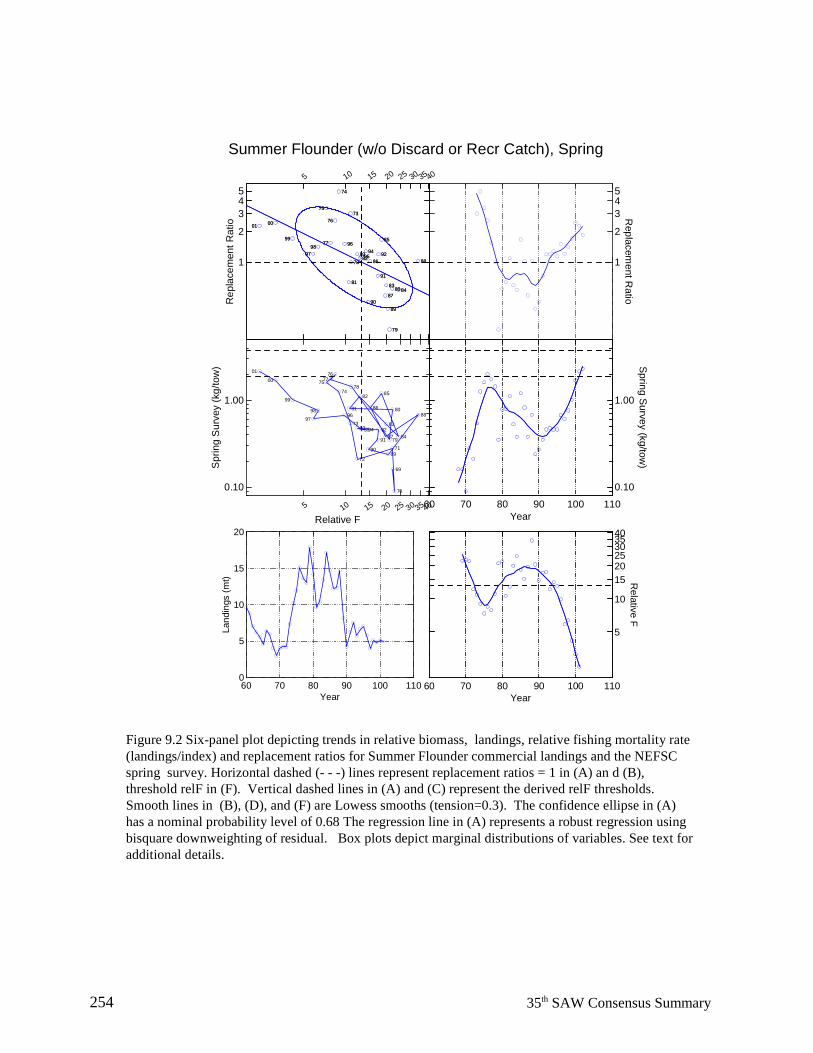
254 35th SAW Consensus Summary
Summer Flounder (w/o Discard or Recr Catch), Spring
1
2
345
Rep
lace
men
t Rat
io 01
88
8480
79
89
83
87
85
92
91
86
90
949582
9378
73
81
96
74
76
77
75
9897
99
00
5 10 15 20 25 30 3540
01
88
8480
79
89
83
87
85
92
91
86
90
949582
9378
73
81
96
74
76
77
75
9897
99
00
5 10 15 20 25 30 3540
Relative F
0.10
1.00
Spr
ing
Sur
vey
(kg/
tow
) 01
88
84
70
69
80
7179
89
83
87
85
92
91
86
90
9495
82
93
72
78
73
8196
74
767775
9897
99
00
60 70 80 90 100 110Year
0
5
10
15
20
Land
ings
(mt)
1
2
345
Replacem
ent Ratio
60 70 80 90 100 110Year
0.10
1.00
Spring Survey (kg/tow)
5
10
152025303540
Relative F
60 70 80 90 100 110Year
Figure 9.2 Six-panel plot depicting trends in relative biomass, landings, relative fishing mortality rate (landings/index) and replacement ratios for Summer Flounder commercial landings and the NEFSC spring survey. Horizontal dashed (- - -) lines represent replacement ratios = 1 in (A) an d (B), threshold relF in (F). Vertical dashed lines in (A) and (C) represent the derived relF thresholds. Smooth lines in (B), (D), and (F) are Lowess smooths (tension=0.3). The confidence ellipse in (A) has a nominal probability level of 0.68 The regression line in (A) represents a robust regression using bisquare downweighting of residual. Box plots depict marginal distributions of variables. See text for additional details.
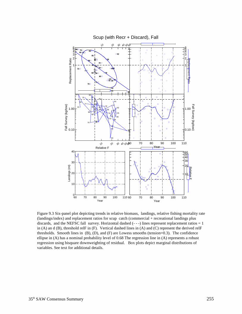
25535th SAW Consensus Summary
Scup (with Recr + Discard), Fall
1
23456
Rep
lace
me n
t Rat
io
00
01
9976
75
77
70
98
69
68
85
84
7473
7297
88
92
89
90
87
91
94
93
8379
95
78
80
81
82
71
96
86
10 20 30 40 50 60
00
01
9976
75
77
70
98
69
68
85
84
7473
7297
88
92
89
90
87
91
94
93
8379
95
78
80
81
82
71
96
86
10 20 30 40 50 60
Relative F
0.10
1.00
Fall
Sur
v ey
(kg/
tow
)
00
01
99
75
77
70
98
69
68
85
847473
72
97
88
65
92
66
64
89
90
67
87
91
94
93
83
79
95
78
80
81
82
7196
86
60 70 80 90 100 110Year
0
10
20
30
40
Land
ings
(mt)
1
23456
Replacem
ent Ratio
60 70 80 90 100 110Year
0.10
1.00
Fall Survey (kg/tow)
10
2030405060
Relative F
60 70 80 90 100 110Year
Figure 9.3 Six-panel plot depicting trends in relative biomass, landings, relative fishing mortality rate (landings/index) and replacement ratios for scup catch (commercial + recreational landings plus discards, and the NEFSC fall survey. Horizontal dashed (- - -) lines represent replacement ratios = 1 in (A) an d (B), threshold relF in (F). Vertical dashed lines in (A) and (C) represent the derived relF thresholds. Smooth lines in (B), (D), and (F) are Lowess smooths (tension=0.3). The confidence ellipse in (A) has a nominal probability level of 0.68 The regression line in (A) represents a robust regression using bisquare downweighting of residual. Box plots depict marginal distributions of variables. See text for additional details.
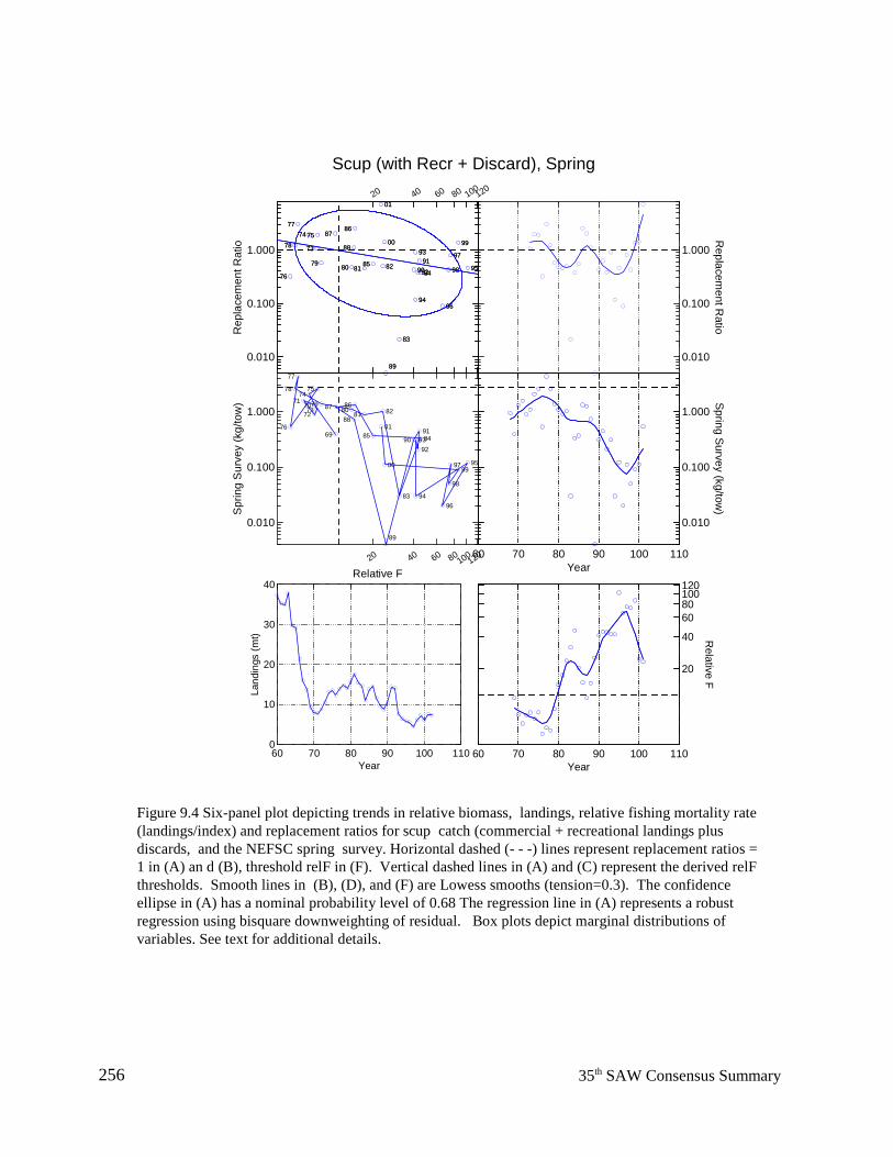
256 35th SAW Consensus Summary
Scup (with Recr + Discard), Spring
0.010
0.100
1.000R
epla
cem
ent R
a tio
76
78
7774
73
75
79
87
95
99
97
98
96
84
9192
94
93
90
83
89
00
82
01
8581
86
88
80
20 40 60 80 100120
76
78
7774
73
75
79
87
95
99
97
98
96
84
9192
94
93
90
83
89
00
82
01
8581
86
88
80
20 40 60 80100120
Relative F
0.010
0.100
1.000
Spr
ing
Sur
vey
(kg/
tow
)
76
78
77
7174
727073
75
79 87
9599
97
98
96
8491
92
94
9390
83
89
00
82
0185
8186
8880
69
60 70 80 90 100 110Year
0
10
20
30
40
Land
ings
(mt)
0.010
0.100
1.000
Replacem
ent Ratio
60 70 80 90 100 110Year
0.010
0.100
1.000
Spring Survey (kg/tow)
20
40
6080100120
Relative F
60 70 80 90 100 110Year
Figure 9.4 Six-panel plot depicting trends in relative biomass, landings, relative fishing mortality rate (landings/index) and replacement ratios for scup catch (commercial + recreational landings plus discards, and the NEFSC spring survey. Horizontal dashed (- - -) lines represent replacement ratios = 1 in (A) an d (B), threshold relF in (F). Vertical dashed lines in (A) and (C) represent the derived relF thresholds. Smooth lines in (B), (D), and (F) are Lowess smooths (tension=0.3). The confidence ellipse in (A) has a nominal probability level of 0.68 The regression line in (A) represents a robust regression using bisquare downweighting of residual. Box plots depict marginal distributions of variables. See text for additional details.
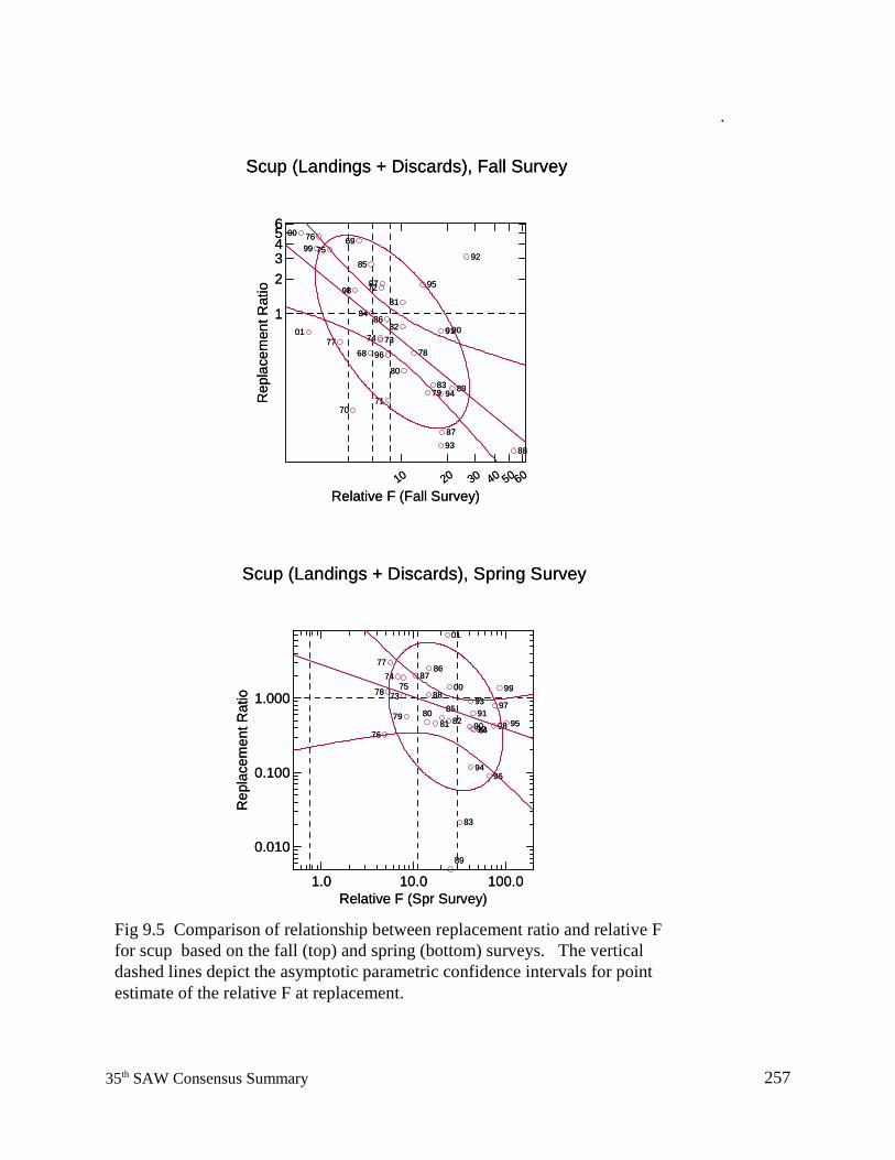
25735th SAW Consensus Summary
Scup (Landings + Discards), Spring Survey
1.0 10.0 100.0Relative F (Spr Survey)
0.010
0.100
1.000
Rep
lace
men
t Rat
io
76
78
7774
7375
79
87
95
99
97
98
96
84
91
92
94
93
90
83
89
00
82
01
85
81
86
88
80
Scup (Landings + Discards), Spring Survey
1.0 10.0 100.0Relative F (Spr Survey)
0.010
0.100
1.000
Rep
lace
men
t Rat
io
76
78
7774
7375
79
87
95
99
97
98
96
84
91
92
94
93
90
83
89
00
82
01
85
81
86
88
80
Scup (Landings + Discards), Fall Survey
10 20 30 40 50 60
Relative F (Fall Survey)
1
23456
Rep
lace
men
t Rat
io
00
01
9976
75
77
70
98
69
68
85
84
74 73
7297
88
92
89
90
87
91
94
93
8379
95
78
80
81
82
71
96
86
Scup (Landings + Discards), Fall Survey
10 20 30 40 50 60
Relative F (Fall Survey)
1
23456
Rep
lace
men
t Rat
io
00
01
9976
75
77
70
98
69
68
85
84
74 73
7297
88
92
89
90
87
91
94
93
8379
95
78
80
81
82
71
96
86
Fig 9.5 Comparison of relationship between replacement ratio and relative F for scup based on the fall (top) and spring (bottom) surveys. The vertical dashed lines depict the asymptotic parametric confidence intervals for point estimate of the relative F at replacement.
.
258
D. SILVER HAKE STOCK IDENTIFICATION
SARC COMMENTS
ObjectivesThe SARC provided technical review of Phoel et al. (2002, SARC WPD1) and provided advice on theimplications of the results for the management of the silver hake stock.
Part I. Silver Hake Abundance and Mid-Atlantic Bight Bottom Water Temperatures
Based on descriptive analysis of survey information, WPD1 concludes that:1. Both commercial landings and survey catches confirm the decrease in silver hake abundance in
the Mid-Atlantic Bight (MAB).2. There is a trend toward warmer bottom water during the spring, albeit only about 1°C increase
in the 33 years studied.3. In both spring and fall, temperatures lie well within the preferred temperature range published for
this species.Despite the lack of hypothesis testing and limitations with temperature data, the conclusions are supportedby temporal patterns in observed survey temperature and biomass indices. However, the SARCquestioned whether the increase in temperature was significant.
Part II. Stock identification of silver hake following Mendelian inheritance and Hardy-Weinberg equilibriumof a microsatellite DNA locus heterogeneity with P2 test for goodness of fit.Major technical problems with genetic analyses, selection of characters and statistical analyses invalidatethe conclusions stated in WPD1: “each sample appears to represent a separate silver hake population.”Silver hake were sampled from the Mid-Atlantic Bight, southern Georges Bank, northern Georges Bank,the Gulf of Maine and the Scotian Shelf. Sample sizes were 14-15 fish from each area. Genotypefrequencies at a single locus were compared to Hardy-Weinberg (H-W) expectations of pooled(combined-area) samples to test for genetic differences among areas using P2 tests (i.e., differences frompooled H-W expectations were used to test that heterogeneous samples were pooled).
Interpretations of allelic frequencies at “locus 4” from PCR images are not appropriate. Primarily, the useof a null allele should be avoided, unless the presence of a such an allele can be confirmed through testing.Analyses should be based on several (4-10) loci with clearly defined bands and several to many allelesfrom many more spawning fish (40-100) for each spawning ground. Secondarily, the statistical tests usedin WPD1 are inappropriate and associated interpretations are incorrect. Using H-W comparisons to detectgroup differences is unconventional and inefficient, because there are many sources of deviation from H-Wequilibrium. More conventional analyses that test for differences among areas should be applied. Othermore appropriate analyses may include genetic distance matrices, molecular variance and phylogenetictrees, such as the analyses presented to the SARC by P. Straub.
25935th SAW Consensus Summary
The samples from each putative stock should be collected over an adequate geographic and temporal rangeto represent each spawning group in order to more closely conform to the assumption of randomness inthe statistical analysis. Existing samples may be available in NMFS archives with associated location, dateand maturity condition.
SARC CONCLUSIONS
Given the deficiencies that were identified in the study, such as the use of a single locus with a null allele andunrepresentative samples, the SARC concluded that the data were inadequate to form reliableinterpretations. Accordingly, the preliminary finding of significant genetic differences among samples shouldbe disregarded. Management units of silver hake should be based on interdisciplinary analysis of publishedstock identification information (e.g., Almeida 1987, Helser et al. 1995, Bolles and Begg 2000). Furtherresearch should address the technical deficiencies of the genetic analyses, sampling design and statisticalmethods.
SOURCES OF INFORMATION
Almeida, F.P. 1987. Stock definition of silver hake in the New England-Middle Atlantic area. N. Am. J.Fish. Manag. 7: 169-186.
Bolles, K.L. and G.A. Begg. 2000. Distinction between silver hake (Merluccius bilinearis) stocks in U.S.waters of the northwest Atlantic based on whole otolith morphometrics. Fish. Bull. 98: 451-462.
Helser, T.E., F.P. Almeida and D.E. Waldron. 1995. Biology and fisheries of North-west Atlantic hake
(silver hake: M. bilinearis) pp203-237 in J. Alheit and T.J. Pitcher, eds. Hake – Biology, Fisheriesand Markets. Chapman and Hall, New York.
Phoel, W.C., J. Lovgren, R.A. Eckhardt, Z.M.G.S. Jahangir, and P.Straub. 2002. The Correlation ofSilver Hake (Merluccius bilinearis) Abundance with Bottom Water Temperatures in the MiddleAtlantic Bight and Stock Identification using Microsatellite DNA. SAW35 WP D1.

Publications and Reportsof the
Northeast Fisheries Science Center
Research Communications UnitNortheast Fisheries Science Center
National Marine Fisheries Service, NOAA166 Water St.
Woods Hole, MA 02543-1026
MEDIA MAIL
The mission of NOAA's National Marine Fisheries Service (NMFS) is "stewardship of living marine resources for the benefit of the nationthrough their science-based conservation and management and promotion of the health of their environment." As the research arm of the NMFS'sNortheast Region, the Northeast Fisheries Science Center (NEFSC) supports the NMFS mission by "planning, developing, and managingmultidisciplinary programs of basic and applied research to: 1) better understand the living marine resources (including marine mammals) ofthe Northwest Atlantic, and the environmental quality essential for their existence and continued productivity; and 2) describe and provide tomanagement, industry, and the public, options for the utilization and conservation of living marine resources and maintenance of environmentalquality which are consistent with national and regional goals and needs, and with international commitments." Results of NEFSC research arelargely reported in primary scientific media (e.g., anonymously-peer-reviewed scientific journals). However, to assist itself in providing data,information, and advice to its constituents, the NEFSC occasionally releases its results in its own media. Those media are in four categories:
NOAA Technical Memorandum NMFS-NE -- This series is issued irregularly. The series typically includes: data reports of long-term field orlab studies of important species or habitats; synthesis reports for important species or habitats; annual reports of overall assessment or monitoringprograms; manuals describing program-wide surveying or experimental techniques; literature surveys of important species or habitat topics;proceedings and collected papers of scientific meetings; and indexed and/or annotated bibliographies. All issues receive internal scientific reviewand most issues receive technical and copy editing.
Northeast Fisheries Science Center Reference Document -- This series is issued irregularly. The series typically includes: data reports on fieldand lab studies; progress reports on experiments, monitoring, and assessments; background papers for, collected abstracts of, and/or summaryreports of scientific meetings; and simple bibliographies. Issues receive internal scientific review, but no technical or copy editing.
Fishermen's Report -- This information report is a quick-turnaround report on the distribution and relative abundance of commercial fisheriesresources as derived from each of the NEFSC's periodic research vessel surveys of the Northeast's continental shelf. There is no scientific review,nor any technical or copy editing, of this report.
The Shark Tagger -- This newsletter is an annual summary of tagging and recapture data on large pelagic sharks as derived from the NMFS'sCooperative Shark Tagging Program; it also presents information on the biology (movement, growth, reproduction, etc.) of these sharks assubsequently derived from the tagging and recapture data. There is internal scientific review, but no technical or copy editing, of this newsletter.
OBTAINING A COPY: To obtain a copy of a NOAA Technical Memorandum NMFS-NE or a Northeast Fisheries Science CenterReference Document, or to subscribe to the Fishermen's Report or the The Shark Tagger, either contact the NEFSC Editorial Office(166 Water St., Woods Hole, MA 02543-1026; 508-495-2228) or consult the NEFSC webpage on "Reports and Publications" (http://www.nefsc.noaa.gov/nefsc/publications/).
ANY USE OF TRADE OR BRAND NAMES IN ANY NEFSC PUBLICATION OR REPORT DOES NOT IMPLYENDORSEMENT.