Embed Size (px)
Citation preview
PERFORMANCE TESTING FOR HOT MIX ASPHALT By
E. Ray Brown
Prithvi S. Kandhal Jingna Zhang
Paper published in Transportation Research Board, Transportation Circular E-C068, September 2004
277 Technology Parkway • Auburn, AL 36830
PERFORMANCE TESTING FOR HOT MIX ASPHALT
By
E. Ray Brown Director
National Center for Asphalt Technology Auburn University, Alabama
Prithvi S. Kandhal
Associate Director Emeritus National Center for Asphalt Technology
Auburn University, Alabama
Jingna Zhang
Visiting Scholar National Center for Asphalt Technology
Auburn University, Alabama
Paper published in Transportation Research Board, Transportation Circular E-C068, September 2004

DISCLAIMER
The contents of this report reflect the views of the authors who are solely responsible for the facts and the accuracy of the data presented herein. The contents do not necessarily reflect the official views and policies of the National Center for Asphalt Technology of Auburn University. This report does not constitute a standard, specification, or regulation.
-i-
TABLE OF CONTENTS Page
List of Tables . . . . . . . . . . . . . . . . . . . . . . . . . . . . . . . . . . . . . . . . . . . . . . . . . . . . . . . . . . . . . . . . iv List of Figures . . . . . . . . . . . . . . . . . . . . . . . . . . . . . . . . . . . . . . . . . . . . . . . . . . . . . . . . . . . . . . . . v Chapter 1. Introduction . . . . . . . . . . . . . . . . . . . . . . . . . . . . . . . . . . . . . . . . . . . . . . . . . . . . . . . . . 1
1.1 Background . . . . . . . . . . . . . . . . . . . . . . . . . . . . . . . . . . . . . . . . . . . . . . . . . . . . . . . . . . . 1 1.2 Objective . . . . . . . . . . . . . . . . . . . . . . . . . . . . . . . . . . . . . . . . . . . . . . . . . . . . . . . . . . . . . 1 1.3 Scope of Study . . . . . . . . . . . . . . . . . . . . . . . . . . . . . . . . . . . . . . . . . . . . . . . . . . . . . . . . . 2
Chapter 2. Descriptions of Distress Mechanisms . . . . . . . . . . . . . . . . . . . . . . . . . . . . . . . . . . . . . 3 2.1 Permanent Deformation . . . . . . . . . . . . . . . . . . . . . . . . . . . . . . . . . . . . . . . . . . . . . . . . . . 3 2.2 Fatigue Cracking . . . . . . . . . . . . . . . . . . . . . . . . . . . . . . . . . . . . . . . . . . . . . . . . . . . . . . . 3 2.3 Low-temperature Cracking . . . . . . . . . . . . . . . . . . . . . . . . . . . . . . . . . . . . . . . . . . . . . . . . 4 2.4 Moisture Susceptibility . . . . . . . . . . . . . . . . . . . . . . . . . . . . . . . . . . . . . . . . . . . . . . . . . . 4 2.5 Friction Properties . . . . . . . . . . . . . . . . . . . . . . . . . . . . . . . . . . . . . . . . . . . . . . . . . . . . . . 4
Chapter 3. Applicable Tests and Response Parameters . . . . . . . . . . . . . . . . . . . . . . . . . . . . . . . . 6 3.1 Test Methods for Permanent Deformation Evaluation . . . . . . . . . . . . . . . . . . . . . . . . . . . 6
3.1.1 Uniaxial and Triaxial Tests . . . . . . . . . . . . . . . . . . . . . . . . . . . . . . . . . . . . . . . . . . 6 3.1.2 Diametral Tests . . . . . . . . . . . . . . . . . . . . . . . . . . . . . . . . . . . . . . . . . . . . . . . . . . 13 3.1.3 Shear Loading Tests . . . . . . . . . . . . . . . . . . . . . . . . . . . . . . . . . . . . . . . . . . . . . . . 14 3.1.4 Empirical Tests . . . . . . . . . . . . . . . . . . . . . . . . . . . . . . . . . . . . . . . . . . . . . . . . . . 19 3.1.5 Simulative Tests . . . . . . . . . . . . . . . . . . . . . . . . . . . . . . . . . . . . . . . . . . . . . . . . . 24
3.2 Fatigue Cracking . . . . . . . . . . . . . . . . . . . . . . . . . . . . . . . . . . . . . . . . . . . . . . . . . . . . . . 37 3.3 Low Temperature (Thermal) Cracking . . . . . . . . . . . . . . . . . . . . . . . . . . . . . . . . . . . . . 39
3.3.1 PG Grading System . . . . . . . . . . . . . . . . . . . . . . . . . . . . . . . . . . . . . . . . . . . . . . . 39 3.3.2. Tests for Low-temperature Properties of Asphalt Binder . . . . . . . . . . . . . . . . . . 39 3.3.3 Dynamic Shear Rheometer (DSR) . . . . . . . . . . . . . . . . . . . . . . . . . . . . . . . . . . . . 39 3.3.4 Bending Beam Rheometer (BBR) . . . . . . . . . . . . . . . . . . . . . . . . . . . . . . . . . . . . 41 3.3.5 Direct Tension Test (DTT) . . . . . . . . . . . . . . . . . . . . . . . . . . . . . . . . . . . . . . . . . 41 3.3.6 AASHTO Standardized Test: Thermal Stress Restrained Specimen Tensile
Strength . . . . . . . . . . . . . . . . . . . . . . . . . . . . . . . . . . . . . . . . . . . . . . . . . . . . . . . . 42 3.4 Moisture-induced Damage (Susceptibility) . . . . . . . . . . . . . . . . . . . . . . . . . . . . . . . . . . 43
3.4.1 Boiling Water Test (ASTM D3625 or a variation) . . . . . . . . . . . . . . . . . . . . . . . 43 3.4.2 Static-Immersion Test (AASHTO T182) . . . . . . . . . . . . . . . . . . . . . . . . . . . . . . . 44 3.4.4 Tunnicliff and Root Conditioning (NCHRP 274) . . . . . . . . . . . . . . . . . . . . . . . . 44 3.4.5 Modified Lottman Test (AASHTO T 283) . . . . . . . . . . . . . . . . . . . . . . . . . . . . . 44 3.4.6 Immersion-Compression Test (AASHTO T 165) . . . . . . . . . . . . . . . . . . . . . . . . 45 3.4.7 SHRP Moisture Susceptibility Study . . . . . . . . . . . . . . . . . . . . . . . . . . . . . . . . . . 45 3.4.8 Net Adsorption Test (NAT) . . . . . . . . . . . . . . . . . . . . . . . . . . . . . . . . . . . . . . . . . 45 3.4.9 Environmental Conditioning System (ECS) . . . . . . . . . . . . . . . . . . . . . . . . . . . . 45 3.4.10 Other Tests . . . . . . . . . . . . . . . . . . . . . . . . . . . . . . . . . . . . . . . . . . . . . . . . . . . . . . 46
3.5 Friction Characteristics . . . . . . . . . . . . . . . . . . . . . . . . . . . . . . . . . . . . . . . . . . . . . . . . . 46 3.5.1 Models for Wet Pavement Friction . . . . . . . . . . . . . . . . . . . . . . . . . . . . . . . . . . . 46 3.5.2 Field and Laboratory Methods . . . . . . . . . . . . . . . . . . . . . . . . . . . . . . . . . . . . . . . 46 3.5.3 British Portable Tester . . . . . . . . . . . . . . . . . . . . . . . . . . . . . . . . . . . . . . . . . . . . . 47 3.5.4 Dynamic Friction Tester (DFTester) . . . . . . . . . . . . . . . . . . . . . . . . . . . . . . . . . . 48
Chapter 4. Comparison of Methods to Evaluate Permanent Deformation . . . . . . . . . . . . . . . . . 50 4.1 Laboratory Validation . . . . . . . . . . . . . . . . . . . . . . . . . . . . . . . . . . . . . . . . . . . . . . . . . . 50
4.1.1 Selection of Materials Used in Project . . . . . . . . . . . . . . . . . . . . . . . . . . . . . . . . 50 4.1.2 Experimental Plan . . . . . . . . . . . . . . . . . . . . . . . . . . . . . . . . . . . . . . . . . . . . . . . . 51 4.1.3 Test Results . . . . . . . . . . . . . . . . . . . . . . . . . . . . . . . . . . . . . . . . . . . . . . . . . . . . . 52
4.2 Assessment of All Available Test Methods . . . . . . . . . . . . . . . . . . . . . . . . . . . . . . . . . . 54
-ii-

Chapter 5. Recommended Procedures to Evaluate and Optimize Performance . . . . . . . . . . . . . 60 5.1 Permanent Deformation . . . . . . . . . . . . . . . . . . . . . . . . . . . . . . . . . . . . . . . . . . . . . . . . . 60 5.2 Fatigue Cracking . . . . . . . . . . . . . . . . . . . . . . . . . . . . . . . . . . . . . . . . . . . . . . . . . . . . . . 61 5.3 Thermal Cracking . . . . . . . . . . . . . . . . . . . . . . . . . . . . . . . . . . . . . . . . . . . . . . . . . . . . . . 61 5.4 Moisture Susceptibility . . . . . . . . . . . . . . . . . . . . . . . . . . . . . . . . . . . . . . . . . . . . . . . . . 61 5.5 Friction Properties . . . . . . . . . . . . . . . . . . . . . . . . . . . . . . . . . . . . . . . . . . . . . . . . . . . . . 61
Chapter 6. References . . . . . . . . . . . . . . . . . . . . . . . . . . . . . . . . . . . . . . . . . . . . . . . . . . . . . . . . . 63 Appendix A: Asphalt Pavement Analyzer . . . . . . . . . . . . . . . . . . . . . . . . . . . . . . . . . . . . . . . . . . 68 Appendix B: Hamburg Wheel-tracking Device . . . . . . . . . . . . . . . . . . . . . . . . . . . . . . . . . . . . . . 69 Appendix C: French Rutting Tester . . . . . . . . . . . . . . . . . . . . . . . . . . . . . . . . . . . . . . . . . . . . . . . 70 Acknowledgments . . . . . . . . . . . . . . . . . . . . . . . . . . . . . . . . . . . . . . . . . . . . . . . . . . . . . . . . . . . . 71
-iii-
LIST OF TABLES Page
Table 3.1: Table 3.2: Table 3.3: Table 4.1: Table 4.2: Table 4.3: Table 4.4: Table 4.5: Table 4.6: Table 4.7: Table 4.7: Table 4.7: Table 4.7: Table 5.1: Table A.1: Table B.1: Table C.1:
Criteria for Evaluating Rut Resistance Using RSCH Permanent Shear Strain . . 17 Comparison of Test Methods for Fatigue Cracking . . . . . . . . . . . . . . . . . . . . . . 38 Representative Friction Measuring Devices . . . . . . . . . . . . . . . . . . . . . . . . . . . . 47 Coarse Aggregate Properties . . . . . . . . . . . . . . . . . . . . . . . . . . . . . . . . . . . . . . . . 50 Fine Aggregate Properties . . . . . . . . . . . . . . . . . . . . . . . . . . . . . . . . . . . . . . . . . . 50 Properties of Asphalt Binder . . . . . . . . . . . . . . . . . . . . . . . . . . . . . . . . . . . . . . . . 51 Aggregate Gradation (12.5 mm Nominal Maximum Aggregate Size) . . . . . . . . 52 Mix Design Volumetric Properties . . . . . . . . . . . . . . . . . . . . . . . . . . . . . . . . . . . 52 Results from the Performance Tests . . . . . . . . . . . . . . . . . . . . . . . . . . . . . . . . . . 53 Comparative Assessment of Test Methods . . . . . . . . . . . . . . . . . . . . . . . . . . . . . 54 Comparative Assessment of Test Methods (continued) . . . . . . . . . . . . . . . . . . . 55 Comparative Assessment of Test Methods (continued) . . . . . . . . . . . . . . . . . . . 56 Comparative Assessment of Test Methods (continued) . . . . . . . . . . . . . . . . . . . 57 Recommended Tests and Criteria for Permanent Deformation . . . . . . . . . . . . . . 60 Description of Available Criteria for APA . . . . . . . . . . . . . . . . . . . . . . . . . . . . . 68 Description of Available Criteria for HWTD . . . . . . . . . . . . . . . . . . . . . . . . . . . 69 Description of Available Criteria for FRT . . . . . . . . . . . . . . . . . . . . . . . . . . . . . . 70
-iv-
LIST OF FIGURES Page
Figure 3.1: Typical Creep Stress and Strain Relationships . . . . . . . . . . . . . . . . . . . . . . . . . . . . . 7 Figure 3.2: Creep Testing . . . . . . . . . . . . . . . . . . . . . . . . . . . . . . . . . . . . . . . . . . . . . . . . . . . . . . . 8 Figure 3.3: Relationship Between Rut Depth, Rut Rate and Permanent Strain . . . . . . . . . . . . . . 9 Figure 3.4: The Repeated Load Triaxial Test . . . . . . . . . . . . . . . . . . . . . . . . . . . . . . . . . . . . . . . . 9 Figure 3.5: Permanent Strain of Core Samples Subjected to Triaxial Repeated Load Test . . . . 11 Figure 3.6: Rut Depth vs Laboratory Strain from Confined Repeated Load Test . . . . . . . . . . . 11 Figure 3.7: Recording of Haversine Load and Strain (Confined and Unconfined) . . . . . . . . . . 12 Figure 3.8: Indirect Tension Test . . . . . . . . . . . . . . . . . . . . . . . . . . . . . . . . . . . . . . . . . . . . . . . . 13 Figure 3.9: Typical Load and Deformation Versus Time Relationships for Repeated-Load Indirect Tension Test . . . . . . . . . . . . . . . . . . . . . . . . . . . . . . . . . . . . . . . . . . . . . . . . . . . . . . . . . . 14 Figure 3.10: Superpave Shear Tester (SST) . . . . . . . . . . . . . . . . . . . . . . . . . . . . . . . . . . . . . . . . 15 Figure 3.11: Typical Repeated Shear at Constant Height Test Data . . . . . . . . . . . . . . . . . . . . . 16 Figure 3.12: Typical RSCH Shear Strain versus Load Cycles . . . . . . . . . . . . . . . . . . . . . . . . . . 17 Figure 3.13: Shear Device Schematic (Delft University of Technology) . . . . . . . . . . . . . . . . . . 19 Figure 3.14: The Marshall Test . . . . . . . . . . . . . . . . . . . . . . . . . . . . . . . . . . . . . . . . . . . . . . . . . . 20 Figure 3.15: Diagrammatic Sketch Showing Principal Features of Hveem Stabilometer . . . . . 22 Figure 3.16: Gyratory Testing Machine . . . . . . . . . . . . . . . . . . . . . . . . . . . . . . . . . . . . . . . . . . . 23 Figure 3.17: Lateral Pressure Indicator . . . . . . . . . . . . . . . . . . . . . . . . . . . . . . . . . . . . . . . . . . . . 24 Figure 3.18: Asphalt Pavement Analyzer . . . . . . . . . . . . . . . . . . . . . . . . . . . . . . . . . . . . . . . . . . 25 Figure 3.19: Georgia Loaded Wheel Tester . . . . . . . . . . . . . . . . . . . . . . . . . . . . . . . . . . . . . . . . 25 Figure 3.20: Typical APA Rut Depth versus Load Cycles . . . . . . . . . . . . . . . . . . . . . . . . . . . . . 26 Figure 3.21: APA Results vs. WesTrack Performance . . . . . . . . . . . . . . . . . . . . . . . . . . . . . . . . 27 Figure 3.22: Field Rut Depth Versus APA (4% air voids, standard PG temperature, standard hose, and cylinders) Test Results (after NCHRP 9-17) . . . . . . . . . . . . . . . . . . . . . . . . . . . . . . . . 28 Figure 3.23: Field Rut Depth Versus APA (5% air voids, standard PG temperature, standard hose, and beams) Test Results (after NCHRP 9-17) . . . . . . . . . . . . . . . . . . . . . . . . . . . . . . . . . . 28 Figure 3.24: Hamburg Wheel-Tracking Device . . . . . . . . . . . . . . . . . . . . . . . . . . . . . . . . . . . . . 29 Figure 3.25: Definition of Results from Hamburg Wheel-Tracking Device . . . . . . . . . . . . . . . 30 Figure 3.26: Hamburg Wheel-Tracking Device Test Results vs. WesTrack Performance . . . . 31 Figure 3.27: French Rutting Tester . . . . . . . . . . . . . . . . . . . . . . . . . . . . . . . . . . . . . . . . . . . . . . . 32 Figure 3.28: French Rutting Tester Results vs. WesTrack Performance . . . . . . . . . . . . . . . . . . 33 Figure 3.29: Purdue University Laboratory Wheel Tracking Device . . . . . . . . . . . . . . . . . . . . . 33 Figure 3.30: PurWheel Test Results vs. WesTrack Performance . . . . . . . . . . . . . . . . . . . . . . . 34 Figure 3.31: Model Mobile Load Simulator . . . . . . . . . . . . . . . . . . . . . . . . . . . . . . . . . . . . . . . . 35 Figure 3.32: Wessex Engineering Dry Wheel Tracker . . . . . . . . . . . . . . . . . . . . . . . . . . . . . . . . 36 Figure 3.33: Rotary Loaded Wheel Tester . . . . . . . . . . . . . . . . . . . . . . . . . . . . . . . . . . . . . . . . . 37 Figure 3.34: Dynamic Shear Rheometer . . . . . . . . . . . . . . . . . . . . . . . . . . . . . . . . . . . . . . . . . . . 40 Figure 3.35: Computation of G* and * . . . . . . . . . . . . . . . . . . . . . . . . . . . . . . . . . . . . . . . . . . . . 40 Figure 3.36: Bending Beam Rheometer . . . . . . . . . . . . . . . . . . . . . . . . . . . . . . . . . . . . . . . . . . . 41 Figure 3.37: Direct Tension . . . . . . . . . . . . . . . . . . . . . . . . . . . . . . . . . . . . . . . . . . . . . . . . . . . . 42 Figure 3.38: Schematic of TSRST System (after SHRP-A-399) . . . . . . . . . . . . . . . . . . . . . . . . 42 Figure 3.39: Typical TSRST Results for Monotonic Cooling (after SHRP-A-399) . . . . . . . . . 43 Figure 3.40: British Portable Tester (BPT) . . . . . . . . . . . . . . . . . . . . . . . . . . . . . . . . . . . . . . . . . 48 Figure 3.41: Dynamic Friction Tester (DFTester) . . . . . . . . . . . . . . . . . . . . . . . . . . . . . . . . . . . 49 Figure 4.1: Laboratory Validation Approach . . . . . . . . . . . . . . . . . . . . . . . . . . . . . . . . . . . . . . . 51 Figure 4.2: Gradation Used in the Project . . . . . . . . . . . . . . . . . . . . . . . . . . . . . . . . . . . . . . . . . 52
-v-
Brown, Kandhal, & Zhang
PERFORMANCE TESTING FOR HOT MIX ASPHALT
E. Ray Brown, Prithvi S. Kandhal, and Jingna Zhang
CHAPTER 1. INTRODUCTION
1.1 BACKGROUND The Superpave Mixture Design and Analysis System was developed in the early 1990's under the Strategic Highway Research Program (SHRP) (1). Originally, the Superpave design method for Hot-Mix Asphalt (HMA) mixtures consisted of three proposed phases: 1) materials selection, 2) aggregate blending, and 3) volumetric analysis on specimens compacted using the Superpave Gyratory Compactor (SGC) (2). It was intended to have a fourth step which would provide a method to analyze the mixture properties and to determine performance potential, however this fourth step is not yet available for adoption. Most highway agencies in the United States have now adopted the volumetric mixture design method. However, as indicated, there is no strength test to compliment the Superpave volumetric mixture design method. The traditional Marshall and Hveem mixture design methods also had associated strength tests. Even though the Marshall and Hveem stability tests were empirical they did provide some measure of the mix quality. There is much work going on to develop a strength test (for example NCHRP 9-19), however, one has not been finalized for adoption at the time this report was prepared and it will likely be several months to years before one is recommended nationally. Considering that approximately 2 million tons of HMA is placed in the U.S. during a typical construction day, contractors and state agencies must have some means as soon as practical to better evaluate performance potential of HMA. These test methods do not have to be perfect but they should be available in the immediate future for assuring good mix performance.
Research from WesTrack, NCHRP 9-7 (Field Procedures and Equipment to Implement SHRP
Asphalt Specifications), and other experimental construction projects have shown that the Superpave volumetric mixture design method alone is not sufficient to ensure reliable mixture performance over a wide range of materials, traffic and climatic conditions. The HMA industry needs a simple performance test to help ensure that a quality product is produced. Controlling volumetric properties alone is not sufficient to ensure good performance.
There are five areas of distress for which guidance is needed: fatigue cracking, rutting, thermal
cracking, friction, and moisture susceptibility. All of these distresses can result in loss of performance but rutting is the one distress that is most likely to be a sudden failure as a result of unsatisfactory hot mix asphalt. Other distresses are typically long term failures that show up after a few years of traffic.
Due to the immediate need for some method to evaluate performance potential, the NCAT Board
of Directors requested that NCAT provide guidance that could improve mixture analysis procedures. It is anticipated that this guidance can be adopted until something better is developed in the future through projects such as NCHRP 9-19 and others. However, partly as a result of warranty work, the best technology presently available needs to be identified and adopted. This report provides a first step in identifying appropriate tests. It is anticipated that the findings in this report will be renewed on a regular basis to determine if improved guidance is available and needs to be implemented.
1.2 OBJECTIVE
The purpose of this project is to evaluate available information on permanent deformation, fatigue cracking, low-temperature cracking, moisture susceptibility, and friction properties, and
1
Brown, Kandhal, & Zhang
as appropriate recommend performance test(s) that can be adopted immediately to ensure
improved performance. Emphasis is placed on permanent deformation.
1.3 SCOPE OF STUDY
The following tasks were conducted to reach the objectives of this project:
Task 1. Conduct a literature search and review the information relevant to the test methods for
evaluating the permanent deformation, fatigue cracking, low-temperature cracking, moisture susceptibility, and friction properties of Hot Mix Asphalt pavements.
Task 2. Compare and assess the available tests regarding specific considerations, such as simplicity, test time, cost of equipment, availability of data to support use, published test method, available criteria, and so on.
Task 3. Select test types with most potential to be used to evaluate mixes to estimate performance of HMA; validate these potential test types based on documented studies and evaluate four mixes with known relative performance in the laboratory to determine if the selected test methods show the right trend in permanent deformation performance. Based upon this assessment, recommend performance test(s).
Task 4. Submit a final report that documents the entire effort. The report should provide the HMA mix designers and QC/QA personnel with the best answers at this time about how to analyze permanent deformation, fatigue cracking, low-temperature cracking, moisture susceptibility and friction properties during mix design and QC/QA. The proposed methods should emphasize QC/QA testing where applicable. The focus of the report is on permanent deformation and all other distresses are secondary. An executive summary of the report will also be prepared.
2
Brown, Kandhal, & Zhang
CHAPTER 2. DESCRIPTIONS OF DISTRESS MECHANISMS
There are many reports that provide much detail on the failure mechanisms for the various HMA distresses. A very brief description of the failure mechanism for each distress is provided below.
2.1 PERMANENT DEFORMATION
Rutting (or permanent deformation) results from the accumulation of small amounts of unrecoverable strain as a result of repeated loads applied to the pavement. Rutting can occur as a result of problems with the subgrade, unbound base course, or HMA. The focus of this effort is permanent deformation caused by HMA mix problems. Permanent deformation in HMA is caused by consolidation and/or lateral movement of the HMA under traffic. Shear failure (lateral movement) of the HMA courses generally occurs in the top 100 mm of the pavement surface (3), however, it can occur deeper if satisfactory materials are not used. Rutting in pavement usually develops gradually with increasing numbers of load applications, typically appearing as longitudinal depressions in the wheel paths sometimes accompanied by small upheavals to the sides. It is typically caused by a combination of densification (decrease in volume and, hence, increase in density) and shear deformation and can occur in any one or more of the HMA layers as well as in the unbound materials underneath the HMA. Eisenmann and Hilmer (4) also found that rutting was mainly caused by deformation flow rather than volume change.
2.2 FATIGUE CRACKING
Fatigue cracking is often called alligator cracking because its closely spaced crack pattern is similar to the pattern on an alligator's back. This type of failure generally occurs when the pavement has been stressed to the limit of its fatigue life by repetitive axle load applications. Fatigue cracking is often associated with loads which are too heavy for the pavement structure or more repetitions of a given load than provided for in design. The problem is often made worse by inadequate pavement drainage which contributes to this distress by allowing the pavement layers to become saturated and lose strength. The HMA layers experience high strains when the underlying layers are weakened by excess moisture and fail prematurely in fatigue. Fatigue cracking can also be caused by repetitive passes with overweight trucks and/or inadequate pavement thickness due to poor quality control during construction (5, 6).
Fatigue cracking can lead to the development of potholes when the individual pieces of HMA
physically separate from the adjacent material and are dislodged from the pavement surface by the action of traffic. Potholes generally occur when fatigue cracking is in the advanced stages and when relatively thin layers of HMA have been used.
Fatigue cracking is generally considered to be more of a structural problem than just a material
problem. It is usually caused by a number of pavement factors that have to occur simultaneously. Obviously, repeated heavy loads must be present. Poor subgrade drainage, resulting in a soft, high deflection pavement, is a principal cause of fatigue cracking. Improperly designed and/or poorly constructed pavement layers that are prone to high deflections when loaded also contribute to fatigue cracking.
In the past, fatigue cracking was thought to initiate from the bottom and migrate toward the
surface. These cracks began because of the high tensile strain at the bottom of the HMA. Recently, fatigue cracks have been observed starting at the surface and migrating downward. The surface cracking starts due to tensile strains in the surface of the HMA. Generally speaking it is believed that for thin pavements the fatigue cracking typically starts at the bottom of the HMA and for thick pavements the fatigue cracking typically starts at the HMA surface. Typically fatigue cracking is not caused by a lack of control of HMA properties, however, these
3
Brown, Kandhal, & Zhang
properties can certainly have a secondary effect.
2.3 LOW-TEMPERATURE CRACKING
Low temperature cracking of asphalt pavements is attributed to tensile strain induced in hot mix asphalt as the temperature drops to some critically low level. As its name indicates, low temperature cracking is a distress type that is caused by low pavement temperatures rather than by applied traffic loads even though traffic loads do likely play a role. Thermal cracking is characterized (6) by intermittent transverse cracks (i.e., perpendicular to the direction of traffic) that may occur at a surprisingly consistent spacing. Low temperature cracks form when an asphalt pavement layer shrinks in cold weather. As the pavement shrinks, tensile strains build within the layer. At some point along the pavement, the tensile stress exceeds the tensile strength and the asphalt layer cracks. Thus, low temperature cracks often occur from a single event of low temperature. Low temperature cracking can also be a fatigue phenomenon resulting from the cumulative effect of many cycles of cold weather. The magnitude and frequency of low temperatures and stiffness of the asphalt mixture on the surface are major factors in the occurrence and intensity of low-temperature transverse cracking. The crack starts at the surface and works its way downward. The mixture stiffness, which is primarily related to the properties of the asphalt binder, is probably the greatest contributer to low-temperature cracking.
2.4 MOISTURE SUSCEPTIBILITY
Environmental factors such as temperature and moisture can have a profound effect on the durability of hot mix asphalt pavements. When critical environmental conditions are coupled with poor materials and traffic, premature failure may result as a result of stripping of the asphalt binder from the aggregate particles.
There are three mechanisms (7) by which moisture can degrade the integrity of a hot mix asphalt
matrix: 1. loss of cohesion (strength) of the asphalt film that may be due to several mechanisms; 2. failure of the adhesion (bond) between the aggregate and asphalt, and 3. degradation or fracture of individual aggregate particles when subjected to freezing.
When the aggregate tends to have a preference for absorbing water, the asphalt is often
"stripped" away. Stripping leads to loss in quality of mixture and ultimately leads to failure of the pavement as a result of raveling, rutting, or cracking.
2.5 FRICTION PROPERTIES
Friction during wet conditions continues to be a major concern of most highway agencies around the world. Recognizing the importance of providing safe pavements for travel during wet weather, most highway agencies have established programs to provide adequate pavement friction or skid resistance (8).
Friction is defined as the relationship between the vertical force and the horizontal force
developed as a tire slides along the pavement surface (5). The friction of a pavement surface is a function of the surface texture which is divided into two components (9, 10, 11), microtexture and macrotexture. The microtexture provides a gritty surface to penetrate thin water films and produce good frictional resistance between the tire and the roadway. The macrotexture provides drainage channels for water expulsion between the tire and the roadway thus allowing better tire contact with the pavement to improve frictional resistance and prevent hydroplaning.
To the vehicle operator, friction is a measure of how quickly a vehicle can be stopped. To the
design engineer, friction is an important safety-related property of the pavement surface that
4

Brown, Kandhal, & Zhang
must be accounted for through proper selection of materials, design, and construction. In terms
of pavement management, friction is a measure of serviceability. The decrease of friction below a minimum acceptable (safe) level prevents the pavement from serving its desired function. In a life cycle cost analysis of pavement performance, restoring friction may need to be considered at some point by the pavement designer and the owner agency. Friction characteristics that are desirable in a good pavement surface are (12):
1.
2.
3.
4.
High friction. Ideally the friction when wet should be as high as possible when compared to that of the dry pavement. Little or no decrease of the friction with increasing speed. The friction of dry pavement is nearly independent of speed, but this is not the case for wet pavement. No reduction in friction with time, from polishing or other causes. Resistance to wear by abrasion of aggregate, attrition of binder or mortar, or loss of particles.
Many states have methods that they have been found successful to ensure good friction with
local materials. Work is needed to develop a national standard to test and evaluate friction properties of hot mix asphalt in the laboratory.
5
Brown, Kandhal, & Zhang
CHAPTER 3. APPLICABLE TESTS AND RESPONSE PARAMETERS
The development of predictive methods or models requires suitable techniques not only for calculating the response of the pavement to load but also for realistically characterizing the materials. The overall objective of materials testing should be to reproduce as closely as practical in situ pavement conditions, including the general stress state, temperature, moisture, and general condition of the material. Mechanistic tests are performed so that expected responses can be determined from any desired loading condition.
3.1 TEST METHODS FOR PERMANENT DEFORMATION EVALUATION
Numerous test methods have been used in the past and are presently being used to characterize the permanent deformation response of asphalt pavement materials. These tests can generally be categorized as:
1. Fundamental Tests:
1) Uniaxial and triaxial tests: unconfined (uniaxial) and confined (triaxial) cylindrical specimens in creep, repeated loading, and strength tests
2) Additional shear tests - shear loading tests: (1) Superpave Shear Tester - Shear Dynamic Modulus (2) Quasi-Direct Shear (Field Shear Test) (3) Superpave Shear Tester - Repeated Shear at Constant Height (4) Direct Shear Test
3) Diametral tests: cylindrical specimens in creep or repeated loading test, strength test
2. Empirical Tests
1) Marshall Test 2) Hveem Test 3) Corps of Engineering Gyratory Testing Machine 4) Lateral Pressure Indicator
3. Simulative Tests
1) Asphalt Pavement Analyzer (new generation of Georgia Loaded Wheel Tester) 2) Hamburg Wheel-Tracking Device 3) French Rutting Tester (LCPC Wheel Tracker) 4) Purdue University Laboratory Wheel Tracking Device 5) Model Mobile Load Simulator 6) Dry Wheel Tracker (Wessex Engineering) 7) Rotary Loaded Wheel Tester (Rutmeter)
3.1.1 Uniaxial and Triaxial Tests
The creep test (unconfined or confined) has been used to estimate the rutting potential of HMA mixtures. This test is conducted by applying a static load to a HMA specimen and measuring the resulting permanent deformation. A typical creep plot is shown in Figure 3.1.
Extensive studies using the unconfined creep test (also known as simple creep test or uniaxial
creep test) as a basis of predicting permanent deformation in HMA have been conducted (13, 14, 15). It has been found that the creep test must be performed at relatively low stress levels (cannot usually exceed 30 psi (206.9 kPa)) and low temperature (cannot usually exceed 104°F (40°C)), otherwise the sample fails prematurely. The test conditions consist of a static axial stress, F, of 100 kPa being applied to a specimen for a period of 1 hour at a temperature of 40/C. These test conditions were standardized following a seminar in Zurich in 1977 (16). This test is inexpensive
6
Brown, Kandhal, & Zhang
and easy to conduct but the ability of the test to predict performance is questionable. In-place
asphalt mixtures are typically exposed to truck tire pressures of approximately 120 psi (828 kPa) and maximum temperatures of 140/F (60/C) or higher (5). Therefore, the conditions of this test do not closely simulate in-place conditions.
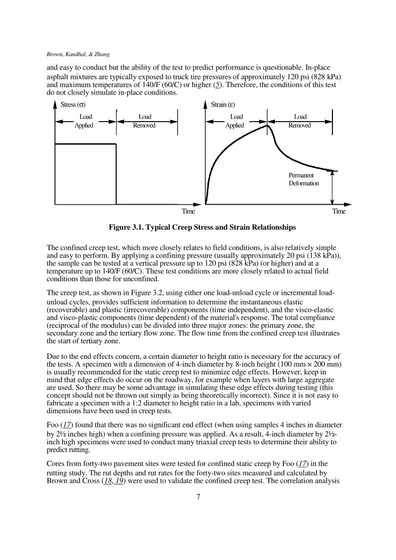
Stress (σ) Strain (ε)
Load Load Load Load Applied Removed Applied Removed
Permanent Deformation
Time Time
Figure 3.1. Typical Creep Stress and Strain Relationships
The confined creep test, which more closely relates to field conditions, is also relatively simple and easy to perform. By applying a confining pressure (usually approximately 20 psi (138 kPa)), the sample can be tested at a vertical pressure up to 120 psi (828 kPa) (or higher) and at a temperature up to 140/F (60/C). These test conditions are more closely related to actual field conditions than those for unconfined.
The creep test, as shown in Figure 3.2, using either one load-unload cycle or incremental load-
unload cycles, provides sufficient information to determine the instantaneous elastic (recoverable) and plastic (irrecoverable) components (time independent), and the visco-elastic and visco-plastic components (time dependent) of the material's response. The total compliance (reciprocal of the modulus) can be divided into three major zones: the primary zone, the secondary zone and the tertiary flow zone. The flow time from the confined creep test illustrates the start of tertiary zone. Due to the end effects concern, a certain diameter to height ratio is necessary for the accuracy of the tests. A specimen with a dimension of 4-inch diameter by 8-inch height (100 mm × 200 mm) is usually recommended for the static creep test to minimize edge effects. However, keep in mind that edge effects do occur on the roadway, for example when layers with large aggregate are used. So there may be some advantage in simulating these edge effects during testing (this concept should not be thrown out simply as being theoretically incorrect). Since it is not easy to fabricate a specimen with a 1:2 diameter to height ratio in a lab, specimens with varied dimensions have been used in creep tests.
Foo (17) found that there was no significant end effect (when using samples 4 inches in diameter
by 2½ inches high) when a confining pressure was applied. As a result, 4-inch diameter by 2½- inch high specimens were used to conduct many triaxial creep tests to determine their ability to predict rutting.
Cores from forty-two pavement sites were tested for confined static creep by Foo (17) in the
rutting study. The rut depths and rut rates for the forty-two sites measured and calculated by Brown and Cross (18, 19) were used to validate the confined creep test. The correlation analysis
7
Brown, Kandhal, & Zhang
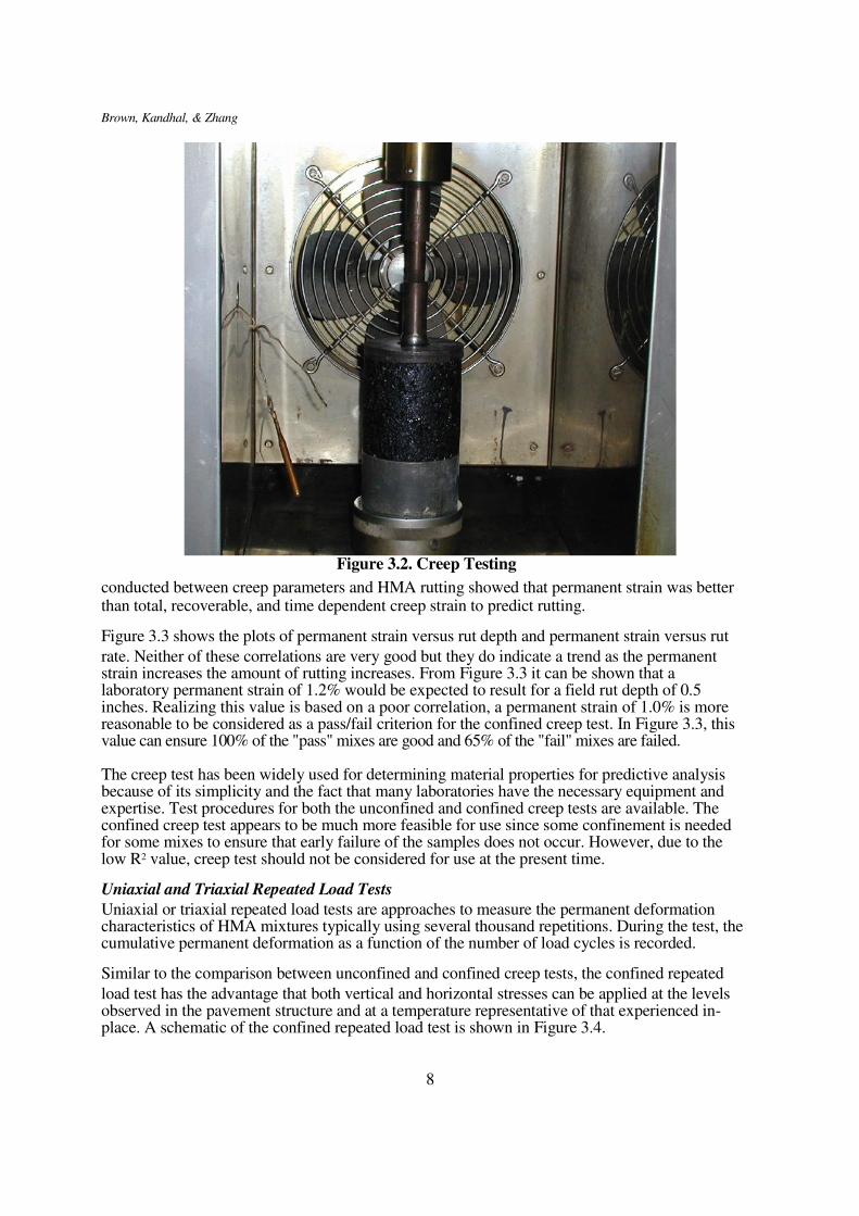
Figure 3.2. Creep Testing
conducted between creep parameters and HMA rutting showed that permanent strain was better than total, recoverable, and time dependent creep strain to predict rutting.
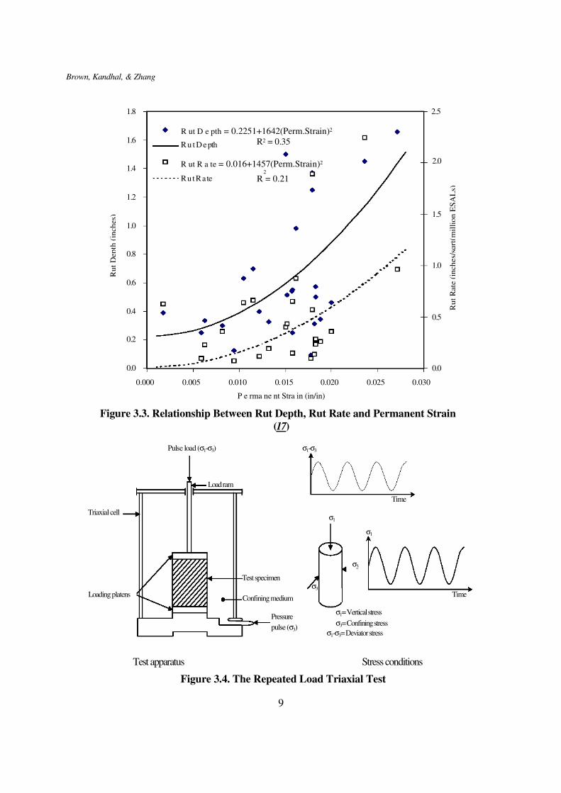
Figure 3.3 shows the plots of permanent strain versus rut depth and permanent strain versus rut
rate. Neither of these correlations are very good but they do indicate a trend as the permanent strain increases the amount of rutting increases. From Figure 3.3 it can be shown that a laboratory permanent strain of 1.2% would be expected to result for a field rut depth of 0.5 inches. Realizing this value is based on a poor correlation, a permanent strain of 1.0% is more reasonable to be considered as a pass/fail criterion for the confined creep test. In Figure 3.3, this value can ensure 100% of the "pass" mixes are good and 65% of the "fail" mixes are failed. The creep test has been widely used for determining material properties for predictive analysis because of its simplicity and the fact that many laboratories have the necessary equipment and expertise. Test procedures for both the unconfined and confined creep tests are available. The confined creep test appears to be much more feasible for use since some confinement is needed for some mixes to ensure that early failure of the samples does not occur. However, due to the low R2 value, creep test should not be considered for use at the present time.
Uniaxial and Triaxial Repeated Load Tests
Uniaxial or triaxial repeated load tests are approaches to measure the permanent deformation characteristics of HMA mixtures typically using several thousand repetitions. During the test, the cumulative permanent deformation as a function of the number of load cycles is recorded.
Similar to the comparison between unconfined and confined creep tests, the confined repeated
load test has the advantage that both vertical and horizontal stresses can be applied at the levels observed in the pavement structure and at a temperature representative of that experienced in- place. A schematic of the confined repeated load test is shown in Figure 3.4.
8
Brown, Kandhal, & Zhang
1.8 2.5
R ut D e pth = 0.2251+1642(Perm.Strain)2
1.6 R u t D e pth R2 = 0.35
1.4
R ut R a te = 0.016+1457(Perm.Strain)2 2
2.0
1.2
1.0
0.8
0.6
0.4
0.2
0.0
R u t R a te R = 0.21 1.5 1.0 0.5 0.0
0.000 0.005 0.010 0. 015 0.020 0.025 0.030
P e rma ne nt Stra in (in/in)
Figure 3.3. Relationship Between Rut Depth, Rut Rate and Permanent Strain
(17)
Pulse load (σ1-σ3) σ1-σ3
Triaxial cell
Loading platens
Load ram
Test specimen Confining medium
σ3
σ1
σ3
σ1
Time
Time
Pressure pulse (σ3)
σ1= Vertical stress σ3= Confining stress
σ1-σ3= Deviator stress
Test apparatus Stress conditions
Figure 3.4. The Repeated Load Triaxial Test
9
Ru
t R
ate
(in
ches
/sq
rt(m
illi
on
ES
AL
s)
Ru
t D
epth
(in
ches
)
Brown, Kandhal, & Zhang
Results from repeated load tests typically are presented in terms of the cumulative permanent
strain versus the number of loading cycles. The cumulative permanent strain curve can be divided into three major zones: the primary zone, the secondary zone and the tertiary zone.
Triaxial and uniaxial repeated load tests appear to be more sensitive than the creep test to HMA
mix variables. On the basis of extensive testing, Barksdale (20) reported that triaxial repeated load tests appear to provide a better measure of rutting characteristics than the creep tests. The triaxial repeated load test, conducted on 4-inch diameter by 6-inch height specimens, is being studied by NCHRP 9-19 as one of their top selected simple performance tests for rutting prediction.
Realizing the difficulty of obtaining 4-inch diameter by 6-inch height (or 8-inch height)
specimens, Mallick, Ahlrich, and Brown (21) and Kandhal and Cooley (22) have successfully used other specimen dimensions which are easy to prepare in the lab to study the potential of using triaxial repeated load tests to predict rutting. In their study, a deviator stress along with a confining stress was applied on a 4-inch diameter by 2½-inch height sample for 1 hour, with 0.1- second load duration and 0.9-second rest period intervals. In order to simulate the long-term recovery from the traffic on the HMA mixes, the load was removed and the rebound was measured for 15 minutes. The strain observed at the end of the period was reported as the permanent strain. The permanent strain indicated the rutting potential of the mix.
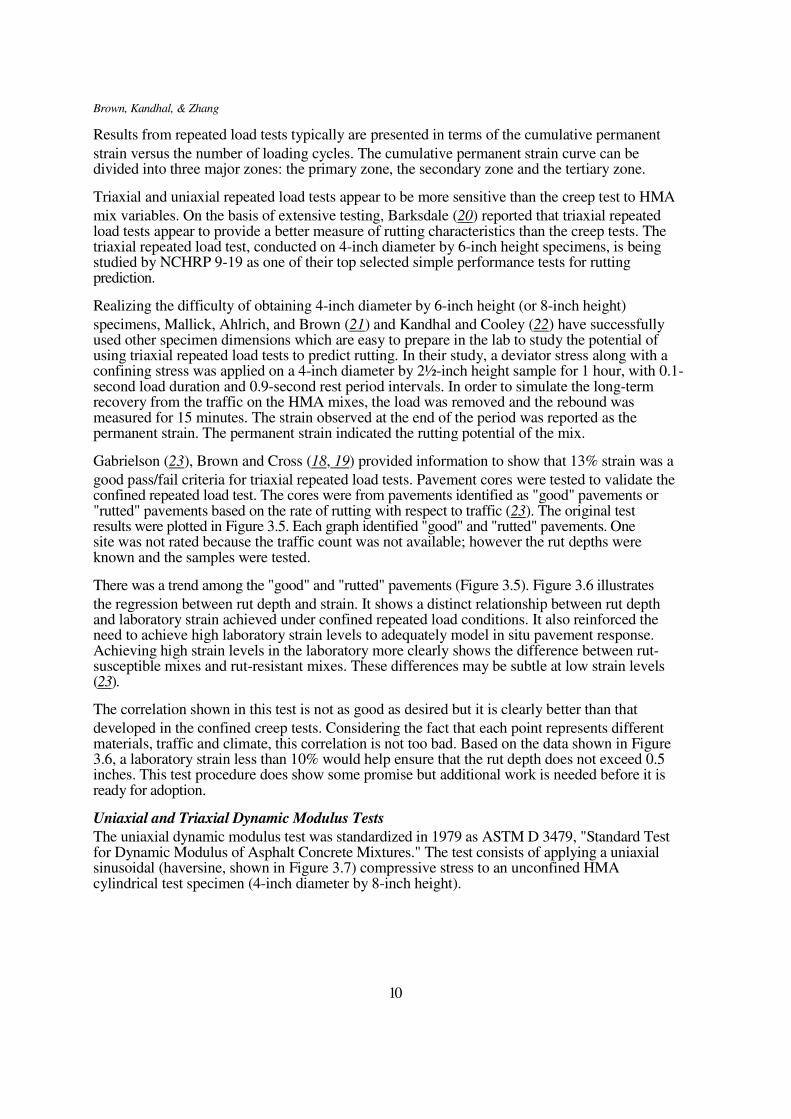
Gabrielson (23), Brown and Cross (18, 19) provided information to show that 13% strain was a
good pass/fail criteria for triaxial repeated load tests. Pavement cores were tested to validate the confined repeated load test. The cores were from pavements identified as "good" pavements or "rutted" pavements based on the rate of rutting with respect to traffic (23). The original test results were plotted in Figure 3.5. Each graph identified "good" and "rutted" pavements. One site was not rated because the traffic count was not available; however the rut depths were known and the samples were tested.
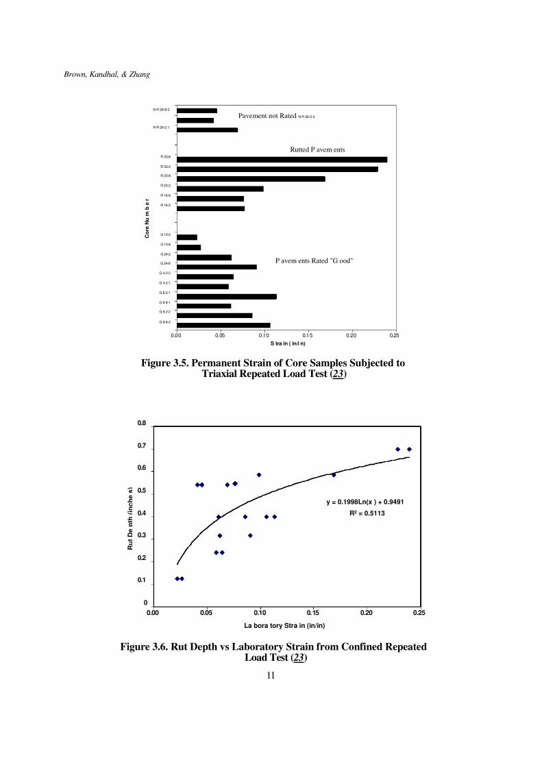
There was a trend among the "good" and "rutted" pavements (Figure 3.5). Figure 3.6 illustrates
the regression between rut depth and strain. It shows a distinct relationship between rut depth and laboratory strain achieved under confined repeated load conditions. It also reinforced the need to achieve high laboratory strain levels to adequately model in situ pavement response. Achieving high strain levels in the laboratory more clearly shows the difference between rut- susceptible mixes and rut-resistant mixes. These differences may be subtle at low strain levels (23).
The correlation shown in this test is not as good as desired but it is clearly better than that
developed in the confined creep tests. Considering the fact that each point represents different materials, traffic and climate, this correlation is not too bad. Based on the data shown in Figure 3.6, a laboratory strain less than 10% would help ensure that the rut depth does not exceed 0.5 inches. This test procedure does show some promise but additional work is needed before it is ready for adoption.
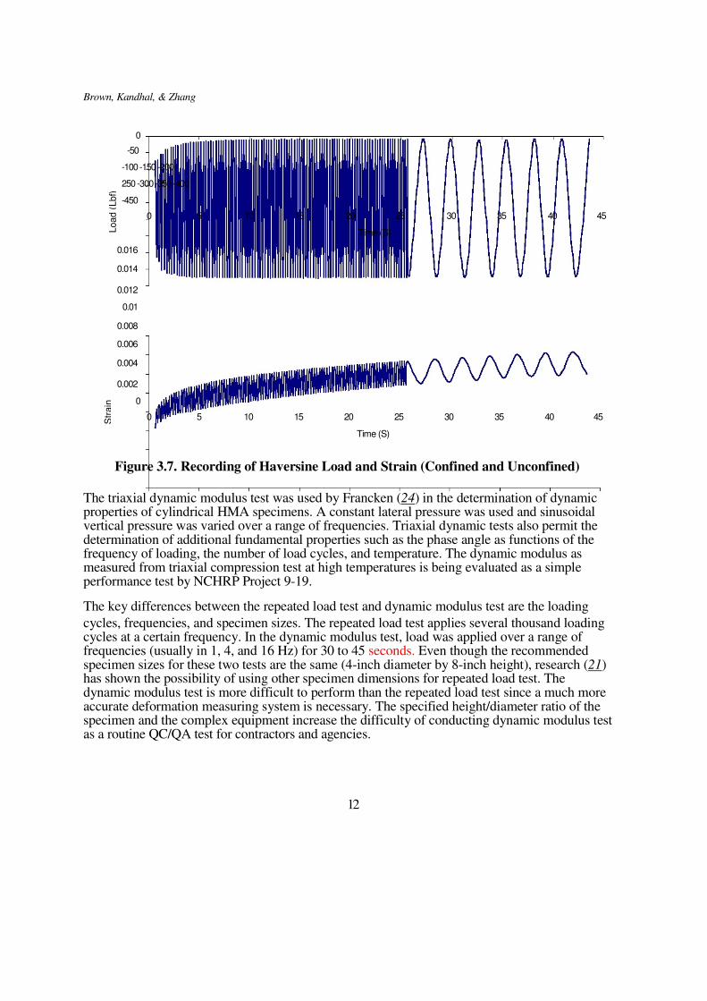
Uniaxial and Triaxial Dynamic Modulus Tests
The uniaxial dynamic modulus test was standardized in 1979 as ASTM D 3479, "Standard Test for Dynamic Modulus of Asphalt Concrete Mixtures." The test consists of applying a uniaxial sinusoidal (haversine, shown in Figure 3.7) compressive stress to an unconfined HMA cylindrical test specimen (4-inch diameter by 8-inch height).
10
Brown, Kandhal, & Zhang
N R 26-8-2 Pavement not Rated N R 26-2-2
N R 26-2-1
R 33-8 R 33-2 R 23-8 R 23-2 R 16-8 R 16-2
Rutted P avem ents
G 10-2 G 10-8 G 24-2
G 24-8
G 4-2-2 G 4-2-1 G 8-2-1 G 8-8-1 G 8-2-2 G 8-8-2
P avem ents Rated "G ood"
0 .0 0 0. 05 0 .1 0 0.1 5 0 .2 0 0.25 S tra in ( in/i n)
Figure 3.5. Permanent Strain of Core Samples Subjected to
Triaxial Repeated Load Test (23)
0.8
0.7
0.6
0.5
0.4
0.3
0.2
0.1
0
y = 0.1998Ln(x ) + 0.9491 R2 = 0.5113
0.00 0.05 0.10 0. 15 0.20 0.25
La bora tory Stra in (in/in)
Figure 3.6. Rut Depth vs Laboratory Strain from Confined Repeated Load Test (23)
11
Co
re N
u m
b e
r
Ru
t D
e p
th (
inch
e s
)
Brown, Kandhal, & Zhang
0 -50
-100 -150 -200 -
250 -300 -350 -400
-450
0 5 10 15 20 25 30 35 40 45
Time (S)
0.016
0.014 0.012
0.01
0.008
0.006
0.004 0.002
0
0 5 10 15 20 25 30 35 40 45
Time (S)
Figure 3.7. Recording of Haversine Load and Strain (Confined and Unconfined)
The triaxial dynamic modulus test was used by Francken (24) in the determination of dynamic properties of cylindrical HMA specimens. A constant lateral pressure was used and sinusoidal vertical pressure was varied over a range of frequencies. Triaxial dynamic tests also permit the determination of additional fundamental properties such as the phase angle as functions of the frequency of loading, the number of load cycles, and temperature. The dynamic modulus as measured from triaxial compression test at high temperatures is being evaluated as a simple performance test by NCHRP Project 9-19.
The key differences between the repeated load test and dynamic modulus test are the loading
cycles, frequencies, and specimen sizes. The repeated load test applies several thousand loading cycles at a certain frequency. In the dynamic modulus test, load was applied over a range of frequencies (usually in 1, 4, and 16 Hz) for 30 to 45 seconds. Even though the recommended specimen sizes for these two tests are the same (4-inch diameter by 8-inch height), research (21) has shown the possibility of using other specimen dimensions for repeated load test. The dynamic modulus test is more difficult to perform than the repeated load test since a much more accurate deformation measuring system is necessary. The specified height/diameter ratio of the specimen and the complex equipment increase the difficulty of conducting dynamic modulus test as a routine QC/QA test for contractors and agencies.
12
Load (
Lbf)
S
train
Brown, Kandhal, & Zhang
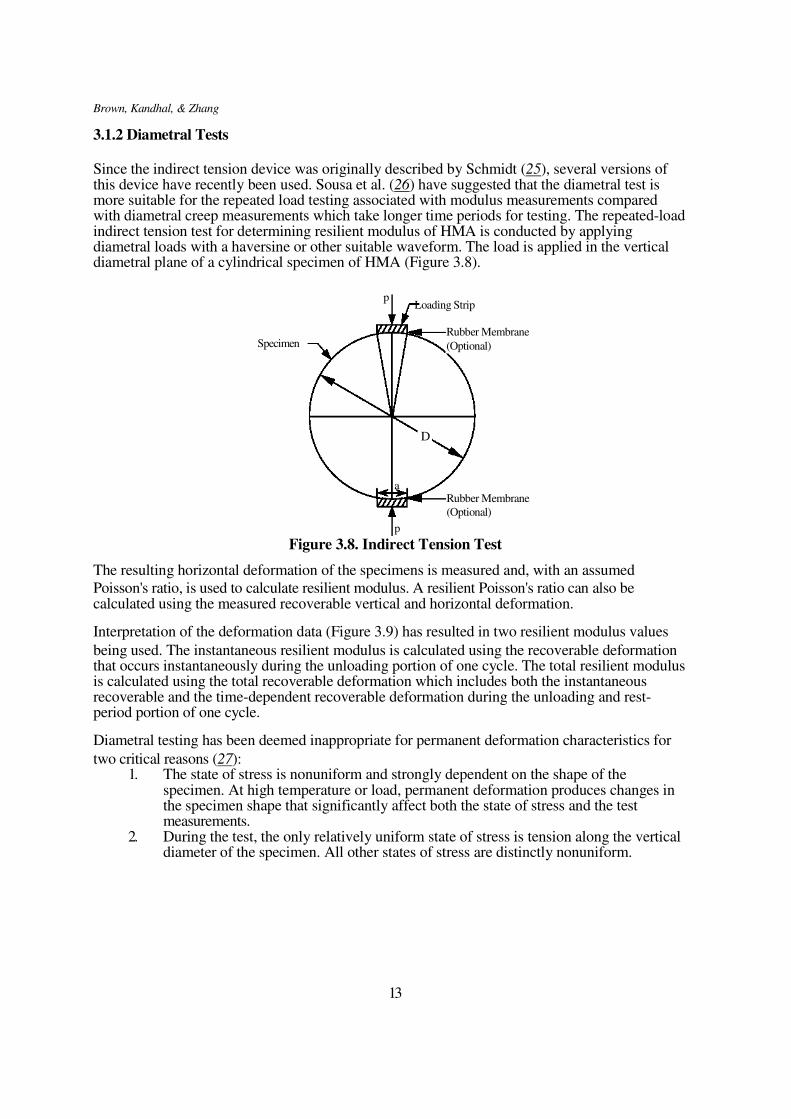
3.1.2 Diametral Tests
Since the indirect tension device was originally described by Schmidt (25), several versions of this device have recently been used. Sousa et al. (26) have suggested that the diametral test is more suitable for the repeated load testing associated with modulus measurements compared with diametral creep measurements which take longer time periods for testing. The repeated-load indirect tension test for determining resilient modulus of HMA is conducted by applying diametral loads with a haversine or other suitable waveform. The load is applied in the vertical diametral plane of a cylindrical specimen of HMA (Figure 3.8).
Specimen
p
Loading Strip
Rubber Membrane (Optional)
D
a Rubber Membrane (Optional)
p
Figure 3.8. Indirect Tension Test
The resulting horizontal deformation of the specimens is measured and, with an assumed
Poisson's ratio, is used to calculate resilient modulus. A resilient Poisson's ratio can also be calculated using the measured recoverable vertical and horizontal deformation.
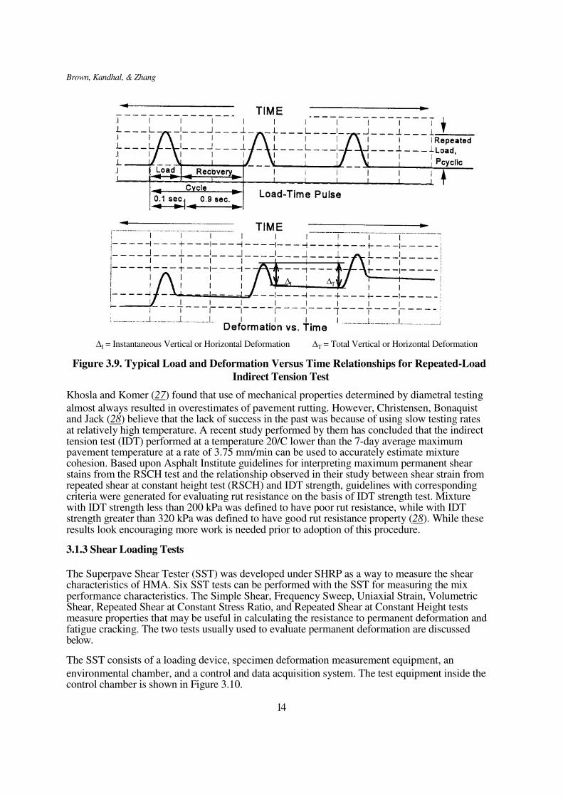
Interpretation of the deformation data (Figure 3.9) has resulted in two resilient modulus values
being used. The instantaneous resilient modulus is calculated using the recoverable deformation that occurs instantaneously during the unloading portion of one cycle. The total resilient modulus is calculated using the total recoverable deformation which includes both the instantaneous recoverable and the time-dependent recoverable deformation during the unloading and rest- period portion of one cycle.
Diametral testing has been deemed inappropriate for permanent deformation characteristics for
two critical reasons (27): 1. 2.
The state of stress is nonuniform and strongly dependent on the shape of the specimen. At high temperature or load, permanent deformation produces changes in the specimen shape that significantly affect both the state of stress and the test measurements. During the test, the only relatively uniform state of stress is tension along the vertical diameter of the specimen. All other states of stress are distinctly nonuniform.
13
Brown, Kandhal, & Zhang
∆I ∆T
∆I = Instantaneous Vertical or Horizontal Deformation ∆T = Total Vertical or Horizontal Deformation
Figure 3.9. Typical Load and Deformation Versus Time Relationships for Repeated-Load
Indirect Tension Test
Khosla and Komer (27) found that use of mechanical properties determined by diametral testing
almost always resulted in overestimates of pavement rutting. However, Christensen, Bonaquist and Jack (28) believe that the lack of success in the past was because of using slow testing rates at relatively high temperature. A recent study performed by them has concluded that the indirect tension test (IDT) performed at a temperature 20/C lower than the 7-day average maximum pavement temperature at a rate of 3.75 mm/min can be used to accurately estimate mixture cohesion. Based upon Asphalt Institute guidelines for interpreting maximum permanent shear stains from the RSCH test and the relationship observed in their study between shear strain from repeated shear at constant height test (RSCH) and IDT strength, guidelines with corresponding criteria were generated for evaluating rut resistance on the basis of IDT strength test. Mixture with IDT strength less than 200 kPa was defined to have poor rut resistance, while with IDT strength greater than 320 kPa was defined to have good rut resistance property (28). While these results look encouraging more work is needed prior to adoption of this procedure.
3.1.3 Shear Loading Tests
The Superpave Shear Tester (SST) was developed under SHRP as a way to measure the shear characteristics of HMA. Six SST tests can be performed with the SST for measuring the mix performance characteristics. The Simple Shear, Frequency Sweep, Uniaxial Strain, Volumetric Shear, Repeated Shear at Constant Stress Ratio, and Repeated Shear at Constant Height tests measure properties that may be useful in calculating the resistance to permanent deformation and fatigue cracking. The two tests usually used to evaluate permanent deformation are discussed below.
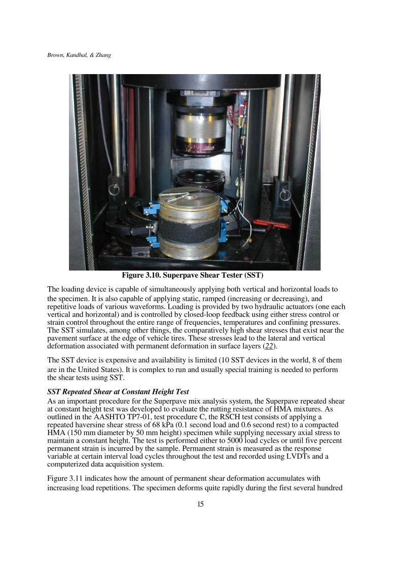
The SST consists of a loading device, specimen deformation measurement equipment, an
environmental chamber, and a control and data acquisition system. The test equipment inside the control chamber is shown in Figure 3.10.
14
Brown, Kandhal, & Zhang
Figure 3.10. Superpave Shear Tester (SST)
The loading device is capable of simultaneously applying both vertical and horizontal loads to
the specimen. It is also capable of applying static, ramped (increasing or decreasing), and repetitive loads of various waveforms. Loading is provided by two hydraulic actuators (one each vertical and horizontal) and is controlled by closed-loop feedback using either stress control or strain control throughout the entire range of frequencies, temperatures and confining pressures. The SST simulates, among other things, the comparatively high shear stresses that exist near the pavement surface at the edge of vehicle tires. These stresses lead to the lateral and vertical deformation associated with permanent deformation in surface layers (22).
The SST device is expensive and availability is limited (10 SST devices in the world, 8 of them
are in the United States). It is complex to run and usually special training is needed to perform the shear tests using SST.
SST Repeated Shear at Constant Height Test
As an important procedure for the Superpave mix analysis system, the Superpave repeated shear at constant height test was developed to evaluate the rutting resistance of HMA mixtures. As outlined in the AASHTO TP7-01, test procedure C, the RSCH test consists of applying a repeated haversine shear stress of 68 kPa (0.1 second load and 0.6 second rest) to a compacted HMA (150 mm diameter by 50 mm height) specimen while supplying necessary axial stress to maintain a constant height. The test is performed either to 5000 load cycles or until five percent permanent strain is incurred by the sample. Permanent strain is measured as the response variable at certain interval load cycles throughout the test and recorded using LVDTs and a computerized data acquisition system.
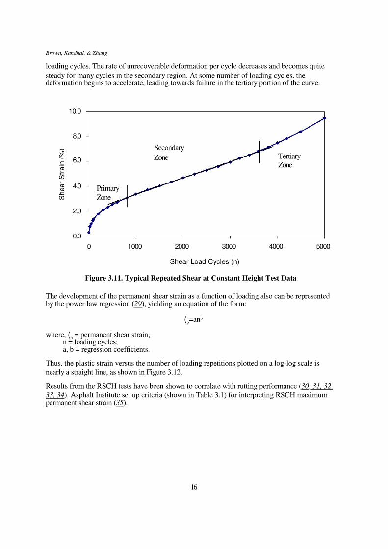
Figure 3.11 indicates how the amount of permanent shear deformation accumulates with
increasing load repetitions. The specimen deforms quite rapidly during the first several hundred
15
Brown, Kandhal, & Zhang
loading cycles. The rate of unrecoverable deformation per cycle decreases and becomes quite
steady for many cycles in the secondary region. At some number of loading cycles, the deformation begins to accelerate, leading towards failure in the tertiary portion of the curve.
10.0
8.0
Secondary
6.0
4.0
2.0
0.0
0
Primary
Zone
1000
Zone 2000
3000
Tertiary Zone
4000
5000
Shear Load Cycles (n)
Figure 3.11. Typical Repeated Shear at Constant Height Test Data
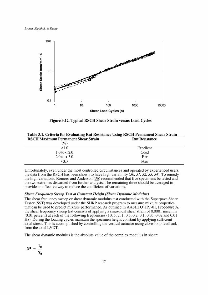
The development of the permanent shear strain as a function of loading also can be represented by the power law regression (29), yielding an equation of the form:
(p=anb
where, (p = permanent shear strain; n = loading cycles; a, b = regression coefficients.
Thus, the plastic strain versus the number of loading repetitions plotted on a log-log scale is
nearly a straight line, as shown in Figure 3.12.
Results from the RSCH tests have been shown to correlate with rutting performance (30, 31, 32,
33, 34). Asphalt Institute set up criteria (shown in Table 3.1) for interpreting RSCH maximum permanent shear strain (35).
16
Sh
ear
Str
ain
(%
)
Brown, Kandhal, & Zhang
10.0
1.0
0.1
1 10 100 1000 10000
Shear Load Cycles (n)
Figure 3.12. Typical RSCH Shear Strain versus Load Cycles
Table 3.1. Criteria for Evaluating Rut Resistance Using RSCH Permanent Shear Strain RSCH Maximum Permanent Shear Strain
(%) < 1.0
1.0 to < 2.0 2.0 to < 3.0
³ 3.0
Rut Resistance
Excellent Good Fair
Poor
Unfortunately, even under the most controlled circumstances and operated by experienced users, the data from the RSCH has been shown to have high variability (30, 31, 32, 33, 34). To remedy the high variations, Romero and Anderson (36) recommended that five specimens be tested and the two extremes discarded from further analysis. The remaining three should be averaged to provide an effective way to reduce the coefficient of variations.
Shear Frequency Sweep Test at Constant Height (Shear Dynamic Modulus)
The shear frequency sweep or shear dynamic modulus test conducted with the Superpave Shear Tester (SST) was developed under the SHRP research program to measure mixture properties that can be used to predict mixture performance. As outlined in AASHTO TP7-01, Procedure A, the shear frequency sweep test consists of applying a sinusoidal shear strain of 0.0001 mm/mm (0.01 percent) at each of the following frequencies (10, 5, 2, 1, 0.5, 0.2, 0.1, 0.05, 0.02 and 0.01 Hz). During the loading cycles maintain the specimen height constant by applying sufficient axial stress. This is accomplished by controlling the vertical actuator using close-loop feedback from the axial LVDT.
The shear dynamic modulus is the absolute value of the complex modulus in shear:
17
Sh
ea
r S
tra
in (
mm
/mm
) %
Brown, Kandhal, & Zhang
Where:
G* = shear dynamic modulus; J0 = peak shear stress amplitude; (0 = peak shear strain amplitude.
Because of the lack of availability and the cost of Superpave shear equipment it is not feasible to
recommend it for immediate use. More information must be developed if it is used effectively in the future.
Quasi- Direct Shear Dynamic Modulus - Field Shear Tester
The Field Shear Tester (FST) was developed through NCHRP 9-7 to control Superpave designed HMA mixtures (37). The device was designed to perform tests comparable to two of the Superpave load related mixture tests: the frequency sweep test at constant height and the simple shear test at constant height (AASHTO TP7-01).
The control software is very similar to the software for the SST and can be used to measure the
dynamic modulus in shear.
In the FST device the specimen is positioned in a similar manner to the indirect tensile test using
loading platens similar to the Marshall test. The test specimen is sheared along its diametral axis by moving a shaft that is attached to the loading frame holding the specimen. In the FST device, the shear frequency sweep test is conducted in a load control method of loading (i.e. applying a constant sinusoidal shear stress and measuring the shear strain as a function of the applied test frequency). As mentioned previously, in the SST device, the shear frequency sweep test is performed in a strain control method of loading (i.e., applying a constant (0.01 percent) sinusoidal shear strain). There are no criteria available in the references for shear dynamic modulus using SST or FST. In order to be used as a performance test for mix design and QC/QA, criteria must be available or sufficient data must be available to develop criteria. Hence, it is recommended that this test not be considered for immediate adoption.
Direct Shear Strength Test
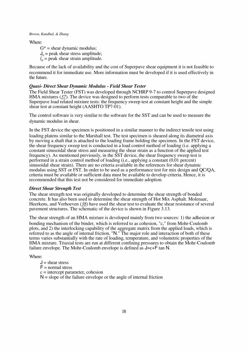
The shear strength test was originally developed to determine the shear strength of bonded concrete. It has also been used to determine the shear strength of Hot Mix Asphalt. Molenaar, Heerkens, and Verhoeven (38) have used the shear test to evaluate the shear resistance of several pavement structures. The schematic of the device is shown in Figure 3.13.
The shear strength of an HMA mixture is developed mainly from two sources: 1) the adhesion or
bonding mechanism of the binder, which is referred to as cohesion, "c," from Mohr-Coulomb plots, and 2) the interlocking capability of the aggregate matrix from the applied loads, which is referred to as the angle of internal friction, "N." The major role and interaction of both of these terms varies substantially with the rate of loading, temperature, and volumetric properties of the HMA mixture. Triaxial tests are run at different confining pressures to obtain the Mohr-Coulomb failure envelope. The Mohr-Coulomb envelope is defined as J=c+F tan N.
Where:
J = shear stress F = normal stress c = intercept parameter, cohesion N = slope of the failure envelope or the angle of internal friction
18
Brown, Kandhal, & Zhang
Figure 3.13. Shear Device Schematic (Delft University of Technology (38))
The direct shear strength test has been used to a much lesser extent than the dynamic modulus and repeated load test in evaluating an HMA mixture's susceptibility to permanent deformation. It appears that insufficient data is available to consider this test for use in predicting performance of HMA.
3.1.4 Empirical Tests
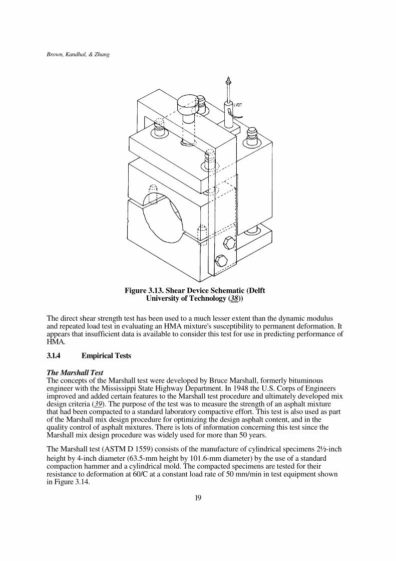
The Marshall Test The concepts of the Marshall test were developed by Bruce Marshall, formerly bituminous engineer with the Mississippi State Highway Department. In 1948 the U.S. Corps of Engineers improved and added certain features to the Marshall test procedure and ultimately developed mix design criteria (39). The purpose of the test was to measure the strength of an asphalt mixture that had been compacted to a standard laboratory compactive effort. This test is also used as part of the Marshall mix design procedure for optimizing the design asphalt content, and in the quality control of asphalt mixtures. There is lots of information concerning this test since the Marshall mix design procedure was widely used for more than 50 years.
The Marshall test (ASTM D 1559) consists of the manufacture of cylindrical specimens 2½-inch
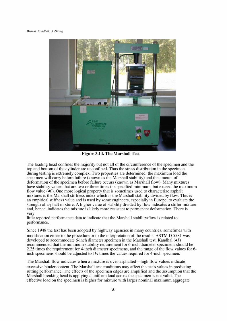
height by 4-inch diameter (63.5-mm height by 101.6-mm diameter) by the use of a standard compaction hammer and a cylindrical mold. The compacted specimens are tested for their resistance to deformation at 60/C at a constant load rate of 50 mm/min in test equipment shown in Figure 3.14.
19
Brown, Kandhal, & Zhang
Figure 3.14. The Marshall Test
The loading head confines the majority but not all of the circumference of the specimen and the top and bottom of the cylinder are unconfined. Thus the stress distribution in the specimen during testing is extremely complex. Two properties are determined: the maximum load the specimen will carry before failure (known as the Marshall stability) and the amount of deformation of the specimen before failure occurs (known as Marshall flow). Many mixtures have stability values that are two or three times the specified minimum, but exceed the maximum flow value (40). One more logical property that is sometimes used to characterize asphalt mixtures is the Marshall stiffness index which is the Marshall stability divided by flow. This is an empirical stiffness value and is used by some engineers, especially in Europe, to evaluate the strength of asphalt mixture. A higher value of stability divided by flow indicates a stiffer mixture and, hence, indicates the mixture is likely more resistant to permanent deformation. There is very little reported performance data to indicate that the Marshall stability/flow is related to performance.
Since 1948 the test has been adopted by highway agencies in many countries, sometimes with
modification either to the procedure or to the interpretation of the results. ASTM D 5581 was developed to accommodate 6-inch diameter specimen in the Marshall test. Kandhal (41) recommended that the minimum stability requirement for 6-inch diameter specimens should be 2.25 times the requirement for 4-inch diameter specimens, and the range of the flow values for 6- inch specimens should be adjusted to 1½ times the values required for 4-inch specimen.
The Marshall flow indicates when a mixture is over-asphalted—high flow values indicate
excessive binder content. The Marshall test conditions may affect the test's values in predicting rutting performance. The effects of the specimen edges are amplified and the assumption that the Marshall breaking head is applying a uniform load across the specimen is not valid. The effective load on the specimen is higher for mixture with larger nominal maximum aggregate
20
Brown, Kandhal, & Zhang
size (40). The Marshall Method has had its shortcomings despite the overall success. Research at
the University of Nottingham (42) showed that the Marshall test is a poor measure of resistance to permanent deformation and may not be able to rank mixes in order of their rut resistance, compared with more realistic repeated load triaxial tests. Other studies have shown similar results.
The Hveem Test
The concepts of the Hveem method of designing paving mixtures were developed under the direction of Francis N. Hveem, a former materials and research engineer for the California Department of Transportation. It is a HMA mixture design tool that was used primarily in the Western United States. The basic philosophy of the Hveem method of mix design was summarized by Vallerga and Lovering (43) as containing the following elements:
1. 2.
3.
It should provide sufficient asphalt cement for aggregate absorption and to produce an optimum film of asphalt cement on the aggregate as determined by the surface area method. It should produce a compacted aggregate-asphalt cement mixture with sufficient stability to resist traffic. It should contain enough asphalt cement for durability from weathering including effects of oxidation and moisture susceptibility.
The Hveem method has been developed over a period of years as certain features have been
improved and other features added. The test procedures and their application have been developed through extensive research and correlation studies on asphalt highway pavements. Similar to the Marshall mix design method, the Hveem method has a large amount of research data available.
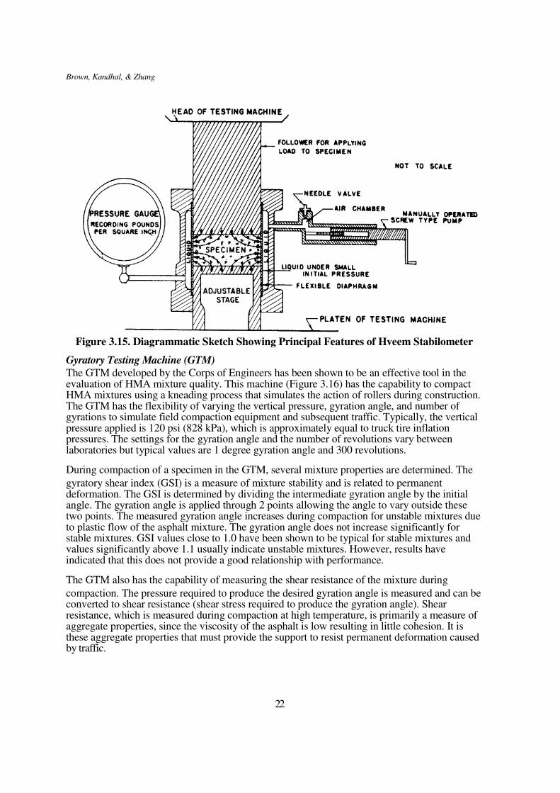
The stabilometer test was developed as an empirical measure of the internal friction within a
mixture. However, the strength or stability of a HMA mixture involves both cohesion and internal friction. Thus, a companion test using the cohesiometer, was developed to measure the cohesion characteristics.
The Hveem method uses standard test specimens of 63.5 mm (2½ in) height by 101.6 mm (4 in)
in diameter. These samples are prepared using a specified procedure for heating, mixing, and compacting the asphalt-aggregate mixtures. In preparing test specimens for the Hveem test, the California Kneading Compactor is normally used. The Hveem stabilometer, shown in Figure 3.15, is a triaxial testing device consisting essentially of a rubber sleeve within a metallic cylinder containing a liquid which registers the horizontal pressure developed by a compacted test specimen as a vertical load is applied. The specimen is maintained in a mold at 60/C (140/F) for the stability test.
The stabilometer values are measurements of internal friction, which are more a reflection of the
properties of the aggregate and the asphalt content than that of the binder grade (40). Stabilometer values are relatively insensitive to asphalt cement characteristics but are indicative of aggregate characteristics. Similar to the Marshall flow values, the Hveem stability does provide an indication when a mixture is over-asphalted—low stability values indicate excessive binder content. Different agencies have modified the Hveem procedure and related equation slightly. Since this test has been replaced with Superpave and there is no significant amount of data to correlate this test with performance, it should not be considered for performance testing.
21
Brown, Kandhal, & Zhang
Figure 3.15. Diagrammatic Sketch Showing Principal Features of Hveem Stabilometer
Gyratory Testing Machine (GTM)
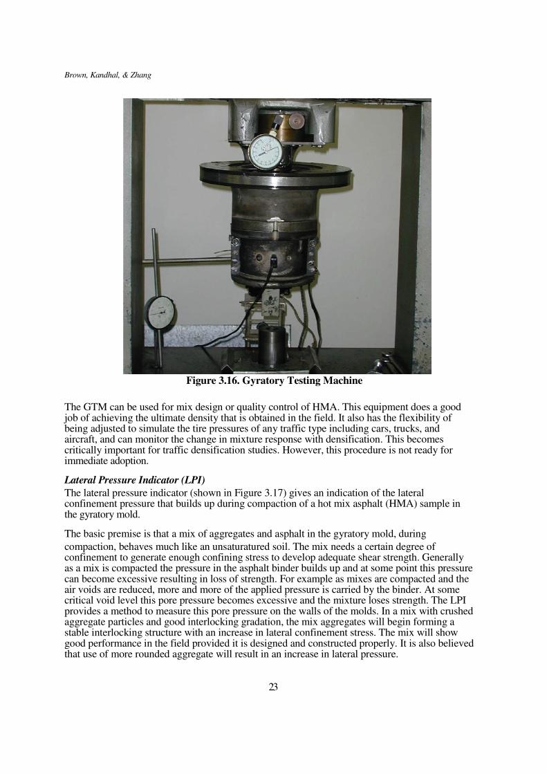
The GTM developed by the Corps of Engineers has been shown to be an effective tool in the evaluation of HMA mixture quality. This machine (Figure 3.16) has the capability to compact HMA mixtures using a kneading process that simulates the action of rollers during construction. The GTM has the flexibility of varying the vertical pressure, gyration angle, and number of gyrations to simulate field compaction equipment and subsequent traffic. Typically, the vertical pressure applied is 120 psi (828 kPa), which is approximately equal to truck tire inflation pressures. The settings for the gyration angle and the number of revolutions vary between laboratories but typical values are 1 degree gyration angle and 300 revolutions.
During compaction of a specimen in the GTM, several mixture properties are determined. The
gyratory shear index (GSI) is a measure of mixture stability and is related to permanent deformation. The GSI is determined by dividing the intermediate gyration angle by the initial angle. The gyration angle is applied through 2 points allowing the angle to vary outside these two points. The measured gyration angle increases during compaction for unstable mixtures due to plastic flow of the asphalt mixture. The gyration angle does not increase significantly for stable mixtures. GSI values close to 1.0 have been shown to be typical for stable mixtures and values significantly above 1.1 usually indicate unstable mixtures. However, results have indicated that this does not provide a good relationship with performance.
The GTM also has the capability of measuring the shear resistance of the mixture during
compaction. The pressure required to produce the desired gyration angle is measured and can be converted to shear resistance (shear stress required to produce the gyration angle). Shear resistance, which is measured during compaction at high temperature, is primarily a measure of aggregate properties, since the viscosity of the asphalt is low resulting in little cohesion. It is these aggregate properties that must provide the support to resist permanent deformation caused by traffic.
22
Brown, Kandhal, & Zhang
Figure 3.16. Gyratory Testing Machine
The GTM can be used for mix design or quality control of HMA. This equipment does a good job of achieving the ultimate density that is obtained in the field. It also has the flexibility of being adjusted to simulate the tire pressures of any traffic type including cars, trucks, and aircraft, and can monitor the change in mixture response with densification. This becomes critically important for traffic densification studies. However, this procedure is not ready for immediate adoption.
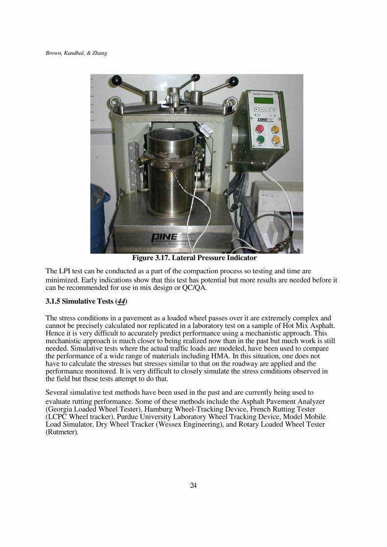
Lateral Pressure Indicator (LPI)
The lateral pressure indicator (shown in Figure 3.17) gives an indication of the lateral confinement pressure that builds up during compaction of a hot mix asphalt (HMA) sample in the gyratory mold.
The basic premise is that a mix of aggregates and asphalt in the gyratory mold, during
compaction, behaves much like an unsaturatured soil. The mix needs a certain degree of confinement to generate enough confining stress to develop adequate shear strength. Generally as a mix is compacted the pressure in the asphalt binder builds up and at some point this pressure can become excessive resulting in loss of strength. For example as mixes are compacted and the air voids are reduced, more and more of the applied pressure is carried by the binder. At some critical void level this pore pressure becomes excessive and the mixture loses strength. The LPI provides a method to measure this pore pressure on the walls of the molds. In a mix with crushed aggregate particles and good interlocking gradation, the mix aggregates will begin forming a stable interlocking structure with an increase in lateral confinement stress. The mix will show good performance in the field provided it is designed and constructed properly. It is also believed that use of more rounded aggregate will result in an increase in lateral pressure.
23
Brown, Kandhal, & Zhang
Figure 3.17. Lateral Pressure Indicator
The LPI test can be conducted as a part of the compaction process so testing and time are
minimized. Early indications show that this test has potential but more results are needed before it can be recommended for use in mix design or QC/QA.
3.1.5 Simulative Tests (44)
The stress conditions in a pavement as a loaded wheel passes over it are extremely complex and cannot be precisely calculated nor replicated in a laboratory test on a sample of Hot Mix Asphalt. Hence it is very difficult to accurately predict performance using a mechanistic approach. This mechanistic approach is much closer to being realized now than in the past but much work is still needed. Simulative tests where the actual traffic loads are modeled, have been used to compare the performance of a wide range of materials including HMA. In this situation, one does not have to calculate the stresses but stresses similar to that on the roadway are applied and the performance monitored. It is very difficult to closely simulate the stress conditions observed in the field but these tests attempt to do that.
Several simulative test methods have been used in the past and are currently being used to
evaluate rutting performance. Some of these methods include the Asphalt Pavement Analyzer (Georgia Loaded Wheel Tester), Hamburg Wheel-Tracking Device, French Rutting Tester (LCPC Wheel tracker), Purdue University Laboratory Wheel Tracking Device, Model Mobile Load Simulator, Dry Wheel Tracker (Wessex Engineering), and Rotary Loaded Wheel Tester (Rutmeter).
24
Brown, Kandhal, & Zhang
Asphalt Pavement Analyzer
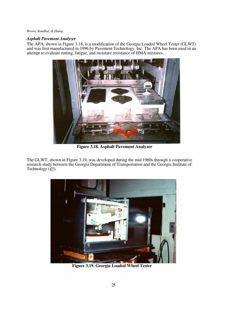
The APA, shown in Figure 3.18, is a modification of the Georgia Loaded Wheel Tester (GLWT) and was first manufactured in 1996 by Pavement Technology, Inc. The APA has been used in an attempt to evaluate rutting, fatigue, and moisture resistance of HMA mixtures.
Figure 3.18. Asphalt Pavement Analyzer
The GLWT, shown in Figure 3.19, was developed during the mid 1980s through a cooperative research study between the Georgia Department of Transportation and the Georgia Institute of Technology (45).
Figure 3.19. Georgia Loaded Wheel Tester
25
Brown, Kandhal, & Zhang
Testing of samples within the GLWT generally consists of applying a 445-N load onto a
pneumatic linear hose pressurized to 690 kPa (100 psi). The load is applied through an aluminum wheel onto the linear hose, which resides on the samples. Test specimens are tracked back and forth under the applied stationary loading. Testing is typically accomplished for a total of 8,000 loading cycles (one cycle is defined as the backward and forward movement over samples by the wheel). However, some researchers have suggested fewer loading cycles may suffice (46).
Since the APA is the second generation of the GLWT, it follows a very similar rut testing
procedure. A loaded wheel is placed on a pressurized linear hose which sits on the test specimens and then tracked back and forth to induce rutting. Similar to the GLWT, most testing in the APA is carried out to 8,000 cycles. Unlike the GLWT, samples also can be tested dry or while submerged in water.
Test specimens for the APA can be either beam or cylindrical. Currently, the most common
method of compacting beam specimens is by the Asphalt Vibratory Compactor (47). However, some have used a linear kneading compactor for beams (48). The most common compactor for cylindrical specimens is the Superpave gyratory compactor (49). Beams are most often compacted to 7 percent air voids; cylindrical samples have been fabricated to both 4 and 7 percent air voids (48). Tests can also be performed on cores or slabs taken from an actual pavement.
Test temperatures for the APA have ranged from 40.6/C to 64/C. The most recent work has been conducted at or near expected maximum pavement temperatures (49, 50).
Wheel load and hose pressure have basically stayed the same as for the GLWT, 445 N and 690
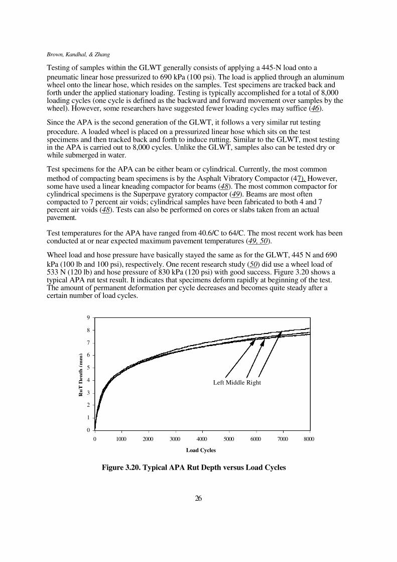
kPa (100 lb and 100 psi), respectively. One recent research study (50) did use a wheel load of 533 N (120 lb) and hose pressure of 830 kPa (120 psi) with good success. Figure 3.20 shows a typical APA rut test result. It indicates that specimens deform rapidly at beginning of the test. The amount of permanent deformation per cycle decreases and becomes quite steady after a certain number of load cycles.
9 8 7 6 5 4 3 2 1 0
Left Middle Right
0 1000 2000 3000 4000 5000 6000 7000 8000
Load Cycles
Figure 3.20. Typical APA Rut Depth versus Load Cycles
26
Ru
T D
epth
(m
m)
Brown, Kandhal, & Zhang
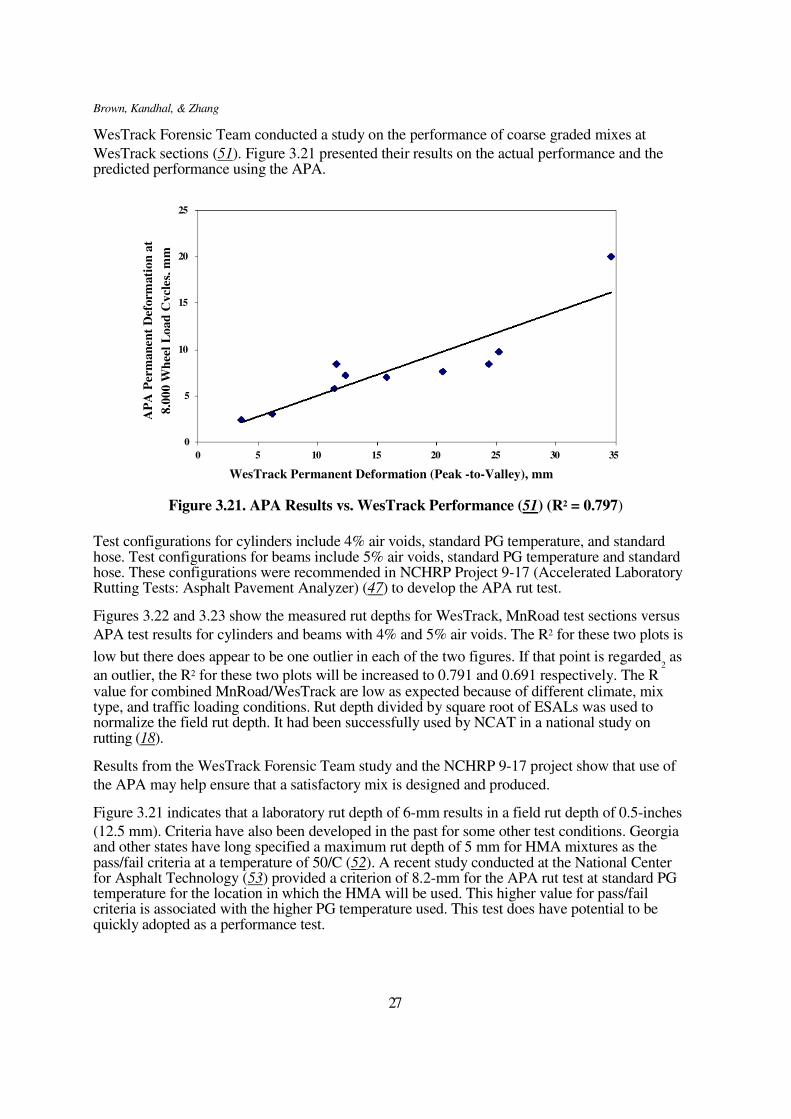
WesTrack Forensic Team conducted a study on the performance of coarse graded mixes at
WesTrack sections (51). Figure 3.21 presented their results on the actual performance and the predicted performance using the APA.
25
20
15
10
5
0
0 5 10 15 20 25 30 35
WesTrack Permanent Deformation (Peak -to-Valley), mm
Figure 3.21. APA Results vs. WesTrack Performance (51) (R2 = 0.797)
Test configurations for cylinders include 4% air voids, standard PG temperature, and standard hose. Test configurations for beams include 5% air voids, standard PG temperature and standard hose. These configurations were recommended in NCHRP Project 9-17 (Accelerated Laboratory Rutting Tests: Asphalt Pavement Analyzer) (47) to develop the APA rut test.
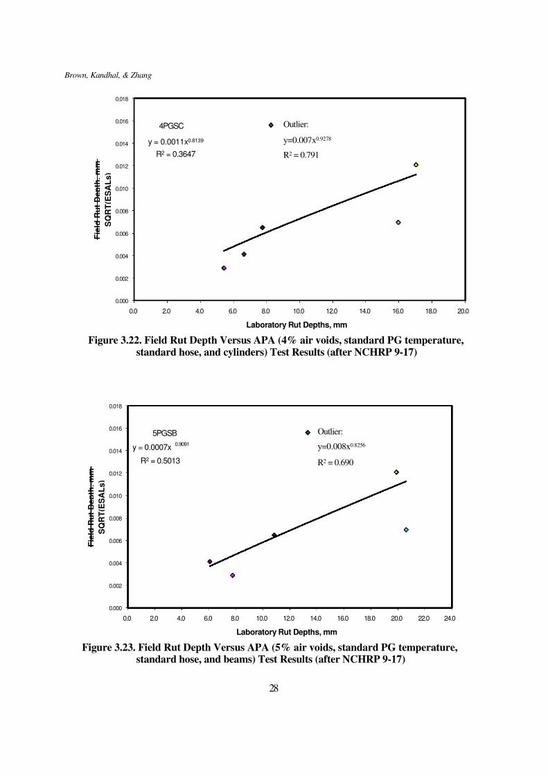
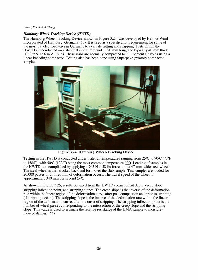
Figures 3.22 and 3.23 show the measured rut depths for WesTrack, MnRoad test sections versus
APA test results for cylinders and beams with 4% and 5% air voids. The R2 for these two plots is
low but there does appear to be one outlier in each of the two figures. If that point is regarded2 as
an outlier, the R2 for these two plots will be increased to 0.791 and 0.691 respectively. The R value for combined MnRoad/WesTrack are low as expected because of different climate, mix type, and traffic loading conditions. Rut depth divided by square root of ESALs was used to normalize the field rut depth. It had been successfully used by NCAT in a national study on rutting (18).
Results from the WesTrack Forensic Team study and the NCHRP 9-17 project show that use of
the APA may help ensure that a satisfactory mix is designed and produced.
Figure 3.21 indicates that a laboratory rut depth of 6-mm results in a field rut depth of 0.5-inches
(12.5 mm). Criteria have also been developed in the past for some other test conditions. Georgia and other states have long specified a maximum rut depth of 5 mm for HMA mixtures as the pass/fail criteria at a temperature of 50/C (52). A recent study conducted at the National Center for Asphalt Technology (53) provided a criterion of 8.2-mm for the APA rut test at standard PG temperature for the location in which the HMA will be used. This higher value for pass/fail criteria is associated with the higher PG temperature used. This test does have potential to be quickly adopted as a performance test.
27
8,0
00 W
hee
l L
oad
Cycl
es,
mm
AP
A P
erm
an
en
t D
eform
ati
on
at
Brown, Kandhal, & Zhang
0.018
0.016
0.014
0.012
0.010
0.008
0.006
0.004
0.002
0.000
4PGSC
y = 0.0011x0.8139
R2 = 0.3647
Outlier:
y=0.007x0.9278
R2 = 0.791
0.0 2.0 4.0 6.0 8.0 10.0 12.0 14.0 16.0 18.0 20.0
Laboratory Rut Depths, mm
Figure 3.22. Field Rut Depth Versus APA (4% air voids, standard PG temperature, standard hose, and cylinders) Test Results (after NCHRP 9-17)
0.018
0.016
5PGSB
Outlier:
0.014
y = 0.0007x 0.9091 y=0.008x0.8256
0.012
0.010
0.008
0.006
0.004
0.002
0.000
R2 = 0.5013 R2 = 0.690
0.0 2.0 4.0 6.0 8.0 10.0 12.0 14.0 16.0 18.0 20.0 22.0 24.0
Laboratory Rut Depths, mm
Figure 3.23. Field Rut Depth Versus APA (5% air voids, standard PG temperature, standard hose, and beams) Test Results (after NCHRP 9-17)
28
SQ
RT
(ES
AL
s)
Fie
ld R
ut
Dep
th,
mm
S
QR
T(E
SA
Ls)
Fie
ld R
ut
Dep
th, m
m
Brown, Kandhal, & Zhang
Hamburg Wheel-Tracking Device (HWTD)
The Hamburg Wheel-Tracking Device, shown in Figure 3.24, was developed by Helmut-Wind Incorporated of Hamburg, Germany (54). It is used as a specification requirement for some of the most traveled roadways in Germany to evaluate rutting and stripping. Tests within the HWTD are conducted on a slab that is 260 mm wide, 320 mm long, and typically 40 mm thick (10.2 in × 12.6 in × 1.6 in). These slabs are normally compacted to 7±1 percent air voids using a linear kneading compactor. Testing also has been done using Superpave gyratory compacted samples.
Figure 3.24. Hamburg Wheel-Tracking Device
Testing in the HWTD is conducted under water at temperatures ranging from 25/C to 70/C (77/F
to 158/F), with 50/C (122/F) being the most common temperature (55). Loading of samples in the HWTD is accomplished by applying a 705 N (158 lb) force onto a 47-mm-wide steel wheel. The steel wheel is then tracked back and forth over the slab sample. Test samples are loaded for 20,000 passes or until 20 mm of deformation occurs. The travel speed of the wheel is approximately 340 mm per second (54).
As shown in Figure 3.25, results obtained from the HWTD consist of rut depth, creep slope,
stripping inflection point, and stripping slopes. The creep slope is the inverse of the deformation rate within the linear region of the deformation curve after post compaction and prior to stripping (if stripping occurs). The stripping slope is the inverse of the deformation rate within the linear region of the deformation curve, after the onset of stripping. The stripping inflection point is the number of wheel passes corresponding to the intersection of the creep slope and the stripping slope. This value is used to estimate the relative resistance of the HMA sample to moisture- induced damage (55).
29
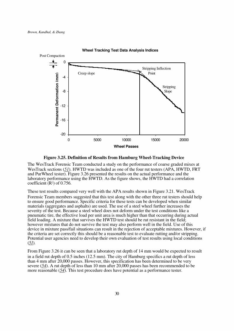
Brown, Kandhal, & Zhang
Wheel Tracking Test Data Analysis Indices
Post Compaction
0
Stripping Inflection
Creep slope Point -4
Stripping -8 Slope
-12
-16
-20
0 5000 10000 15000 20000
Wheel Passes
Figure 3.25. Definition of Results from Hamburg Wheel-Tracking Device
The WesTrack Forensic Team conducted a study on the performance of coarse graded mixes at WesTrack sections (51). HWTD was included as one of the four rut testers (APA, HWTD, FRT and PurWheel tester). Figure 3.26 presented the results on the actual performance and the laboratory performance using the HWTD. As the figure shows, the HWTD had a correlation coefficient (R2) of 0.756.
These test results compared very well with the APA results shown in Figure 3.21. WesTrack
Forensic Team members suggested that this test along with the other three rut testers should help to ensure good performance. Specific criteria for these tests can be developed when similar materials (aggregates and asphalts) are used. The use of a steel wheel further increases the severity of the test. Because a steel wheel does not deform under the test conditions like a pneumatic tire, the effective load per unit area is much higher than that occurring during actual field loading. A mixture that survives the HWTD test should be rut resistant in the field; however mixtures that do not survive the test may also perform well in the field. Use of this device in mixture pass/fail situations can result in the rejection of acceptable mixtures. However, if the criteria are set correctly this should be a reasonable test to evaluate rutting and/or stripping. Potential user agencies need to develop their own evaluation of test results using local conditions (51).
From Figure 3.26 it can be seen that a laboratory rut depth of 14 mm would be expected to result
in a field rut depth of 0.5 inches (12.5 mm). The city of Hamburg specifics a rut depth of less than 4 mm after 20,000 passes. However, this specification has been determined to be very severe (54). A rut depth of less than 10 mm after 20,000 passes has been recommended to be more reasonable (54). This test procedure does have potential as a performance tester.
30
Pe
rma
ne
nt
Defo
rma
tio
n (
mm
)
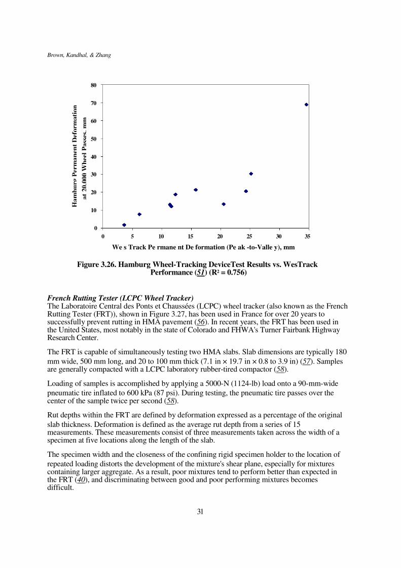
Brown, Kandhal, & Zhang
80
70
60
50
40
30
20
10
0
0 5 10 15 20 25 30 35
We s Track Pe rmane nt De formation (Pe ak -to-Valle y), mm
Figure 3.26. Hamburg Wheel-Tracking DeviceTest Results vs. WesTrack
Performance (51) (R2 = 0.756)
French Rutting Tester (LCPC Wheel Tracker) The Laboratoire Central des Ponts et Chaussées (LCPC) wheel tracker (also known as the French Rutting Tester (FRT)), shown in Figure 3.27, has been used in France for over 20 years to successfully prevent rutting in HMA pavement (56). In recent years, the FRT has been used in the United States, most notably in the state of Colorado and FHWA's Turner Fairbank Highway Research Center.
The FRT is capable of simultaneously testing two HMA slabs. Slab dimensions are typically 180
mm wide, 500 mm long, and 20 to 100 mm thick (7.1 in × 19.7 in × 0.8 to 3.9 in) (57). Samples are generally compacted with a LCPC laboratory rubber-tired compactor (58).
Loading of samples is accomplished by applying a 5000-N (1124-lb) load onto a 90-mm-wide
pneumatic tire inflated to 600 kPa (87 psi). During testing, the pneumatic tire passes over the center of the sample twice per second (58).
Rut depths within the FRT are defined by deformation expressed as a percentage of the original
slab thickness. Deformation is defined as the average rut depth from a series of 15 measurements. These measurements consist of three measurements taken across the width of a specimen at five locations along the length of the slab.
The specimen width and the closeness of the confining rigid specimen holder to the location of
repeated loading distorts the development of the mixture's shear plane, especially for mixtures containing larger aggregate. As a result, poor mixtures tend to perform better than expected in the FRT (40), and discriminating between good and poor performing mixtures becomes difficult.
31
at
20
,000 W
hee
l P
ass
es, m
m
Ha
mb
urg
Per
ma
nen
t D
eform
ati
on
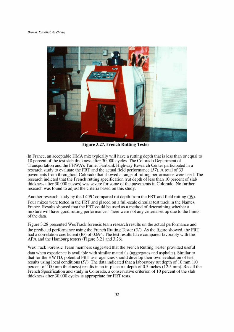
Brown, Kandhal, & Zhang
Figure 3.27. French Rutting Tester
In France, an acceptable HMA mix typically will have a rutting depth that is less than or equal to 10 percent of the test slab thickness after 30,000 cycles. The Colorado Department of Transportation and the FHWA's Turner Fairbank Highway Research Center participated in a research study to evaluate the FRT and the actual field performance (57). A total of 33 pavements from throughout Colorado that showed a range of rutting performance were used. The research indicted that the French rutting specification (rut depth of less than 10 percent of slab thickness after 30,000 passes) was severe for some of the pavements in Colorado. No further research was found to adjust the criteria based on this study.
Another research study by the LCPC compared rut depth from the FRT and field rutting (59).
Four mixes were tested in the FRT and placed on a full-scale circular test track in the Nantes, France. Results showed that the FRT could be used as a method of determining whether a mixture will have good rutting performance. There were not any criteria set up due to the limits of the data.
Figure 3.28 presented WesTrack forensic team research results on the actual performance and
the predicted performance using the French Rutting Tester (51). As the figure showed, the FRT had a correlation coefficient (R2) of 0.694. The test results have compared favorably with the APA and the Hamburg testers (Figure 3.21 and 3.26).
WesTrack Forensic Team members suggested that the French Rutting Tester provided useful
data when experience is available with similar materials (aggregates and asphalts). Similar to that for the HWTD, potential FRT user agencies should develop their own evaluation of test results using local conditions (51). The data indicated that a laboratory rut depth of 10 mm (10 percent of 100 mm thickness) results in an in-place rut depth of 0.5 inches (12.5 mm). Recall the French Specification and study in Colorado, a conservative criterion of 10 percent of the slab thickness after 30,000 cycles is appropriate for FRT tests.
32
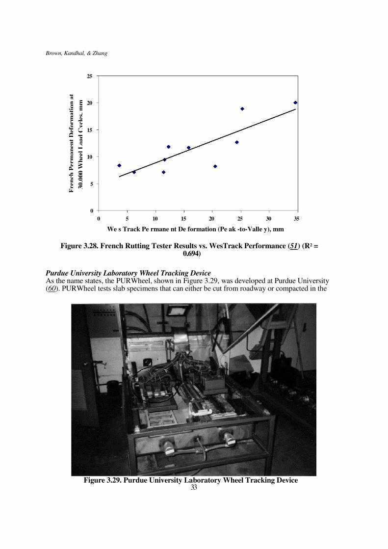
Brown, Kandhal, & Zhang
25
20
15
10
5
0
0 5 10 15 20 25 30 35
We s Track Pe rmane nt De formation (Pe ak -to-Valle y), mm
Figure 3.28. French Rutting Tester Results vs. WesTrack Performance (51) (R2 =
0.694)
Purdue University Laboratory Wheel Tracking Device As the name states, the PURWheel, shown in Figure 3.29, was developed at Purdue University (60). PURWheel tests slab specimens that can either be cut from roadway or compacted in the
Figure 3.29. Purdue University Laboratory Wheel Tracking Device 33
30
,00
0 W
hee
l L
oa
d C
ycl
es, m
m
Fre
nch
Per
ma
nen
t D
eform
ati
on
at
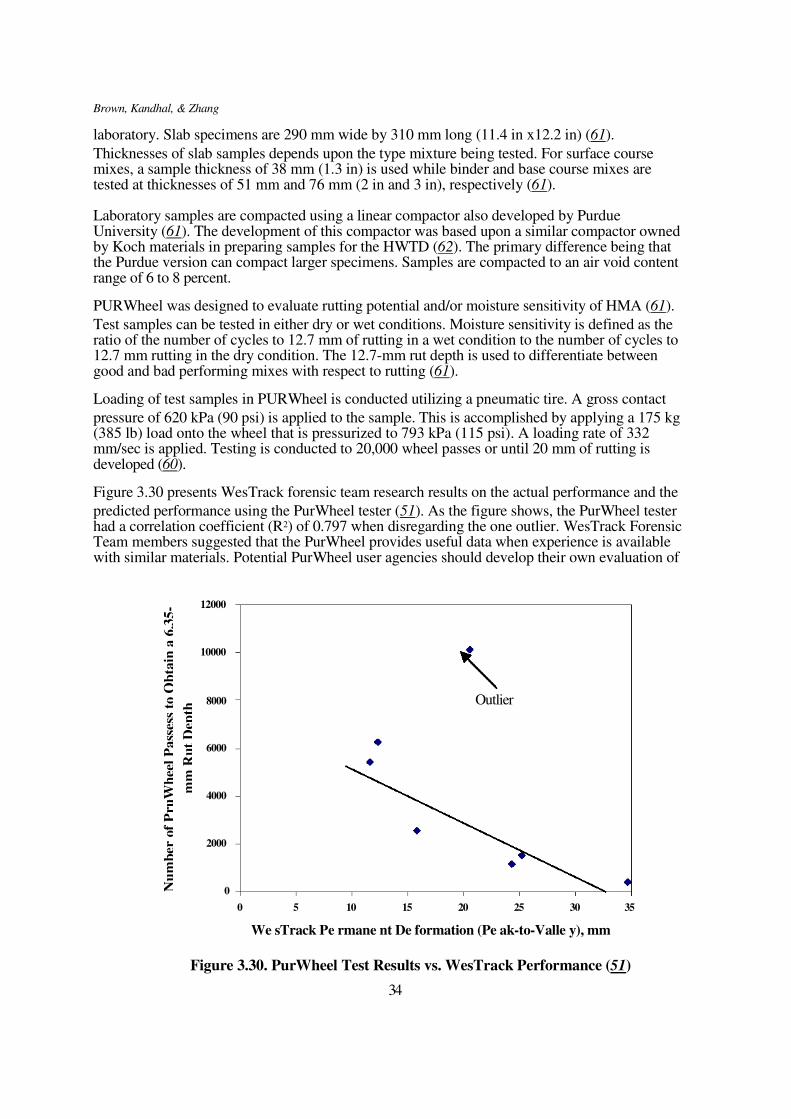
Brown, Kandhal, & Zhang
laboratory. Slab specimens are 290 mm wide by 310 mm long (11.4 in x12.2 in) (61).
Thicknesses of slab samples depends upon the type mixture being tested. For surface course mixes, a sample thickness of 38 mm (1.3 in) is used while binder and base course mixes are tested at thicknesses of 51 mm and 76 mm (2 in and 3 in), respectively (61). Laboratory samples are compacted using a linear compactor also developed by Purdue University (61). The development of this compactor was based upon a similar compactor owned by Koch materials in preparing samples for the HWTD (62). The primary difference being that the Purdue version can compact larger specimens. Samples are compacted to an air void content range of 6 to 8 percent.
PURWheel was designed to evaluate rutting potential and/or moisture sensitivity of HMA (61).
Test samples can be tested in either dry or wet conditions. Moisture sensitivity is defined as the ratio of the number of cycles to 12.7 mm of rutting in a wet condition to the number of cycles to 12.7 mm rutting in the dry condition. The 12.7-mm rut depth is used to differentiate between good and bad performing mixes with respect to rutting (61).
Loading of test samples in PURWheel is conducted utilizing a pneumatic tire. A gross contact
pressure of 620 kPa (90 psi) is applied to the sample. This is accomplished by applying a 175 kg (385 lb) load onto the wheel that is pressurized to 793 kPa (115 psi). A loading rate of 332 mm/sec is applied. Testing is conducted to 20,000 wheel passes or until 20 mm of rutting is developed (60).
Figure 3.30 presents WesTrack forensic team research results on the actual performance and the
predicted performance using the PurWheel tester (51). As the figure shows, the PurWheel tester had a correlation coefficient (R2) of 0.797 when disregarding the one outlier. WesTrack Forensic Team members suggested that the PurWheel provides useful data when experience is available with similar materials. Potential PurWheel user agencies should develop their own evaluation of
12000
10000
8000 Outlier
6000
4000
2000
0 0 5 10 15 20 25 30 35
We sTrack Pe rmane nt De formation (Pe ak-to-Valle y), mm
Figure 3.30. PurWheel Test Results vs. WesTrack Performance (51)
34
mm
Ru
t D
epth
Nu
mb
er o
f P
ruW
hee
l P
ass
ess
to O
bta
in a
6.3
5-
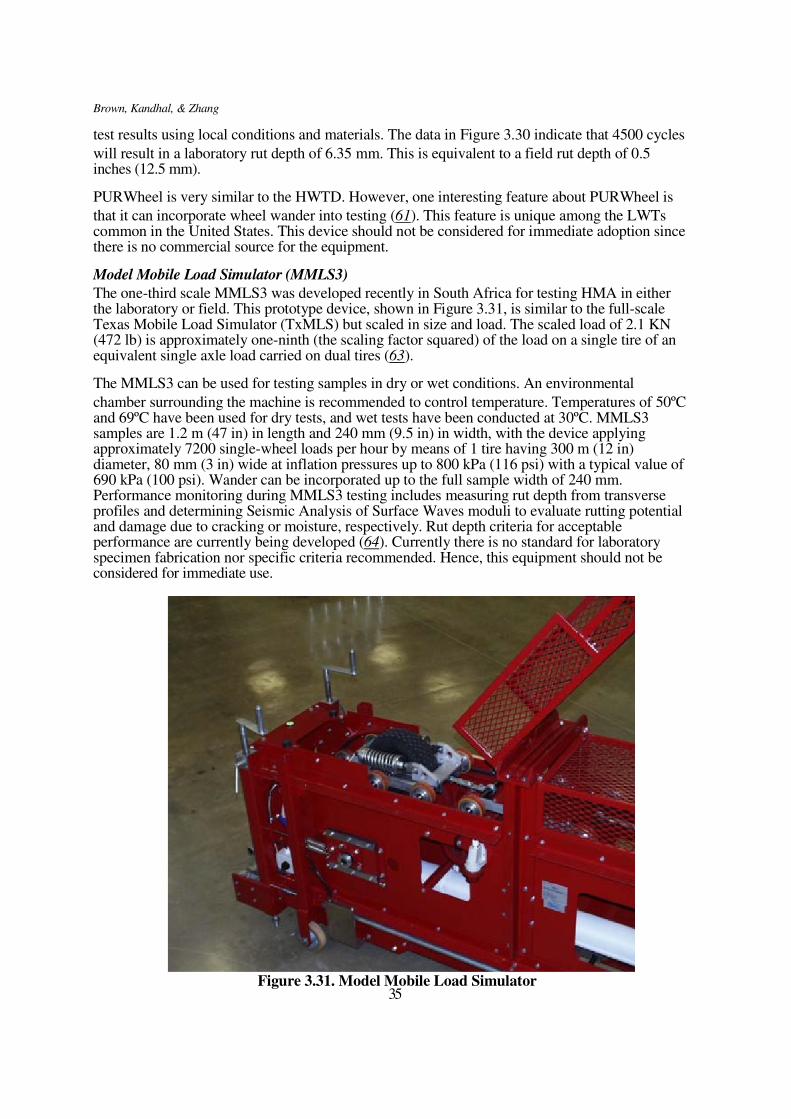
Brown, Kandhal, & Zhang
test results using local conditions and materials. The data in Figure 3.30 indicate that 4500 cycles
will result in a laboratory rut depth of 6.35 mm. This is equivalent to a field rut depth of 0.5 inches (12.5 mm).
PURWheel is very similar to the HWTD. However, one interesting feature about PURWheel is
that it can incorporate wheel wander into testing (61). This feature is unique among the LWTs common in the United States. This device should not be considered for immediate adoption since there is no commercial source for the equipment.
Model Mobile Load Simulator (MMLS3)
The one-third scale MMLS3 was developed recently in South Africa for testing HMA in either the laboratory or field. This prototype device, shown in Figure 3.31, is similar to the full-scale Texas Mobile Load Simulator (TxMLS) but scaled in size and load. The scaled load of 2.1 KN (472 lb) is approximately one-ninth (the scaling factor squared) of the load on a single tire of an equivalent single axle load carried on dual tires (63).
The MMLS3 can be used for testing samples in dry or wet conditions. An environmental
chamber surrounding the machine is recommended to control temperature. Temperatures of 50ºC and 69ºC have been used for dry tests, and wet tests have been conducted at 30ºC. MMLS3 samples are 1.2 m (47 in) in length and 240 mm (9.5 in) in width, with the device applying approximately 7200 single-wheel loads per hour by means of 1 tire having 300 m (12 in) diameter, 80 mm (3 in) wide at inflation pressures up to 800 kPa (116 psi) with a typical value of 690 kPa (100 psi). Wander can be incorporated up to the full sample width of 240 mm. Performance monitoring during MMLS3 testing includes measuring rut depth from transverse profiles and determining Seismic Analysis of Surface Waves moduli to evaluate rutting potential and damage due to cracking or moisture, respectively. Rut depth criteria for acceptable performance are currently being developed (64). Currently there is no standard for laboratory specimen fabrication nor specific criteria recommended. Hence, this equipment should not be considered for immediate use.
Figure 3.31. Model Mobile Load Simulator 35
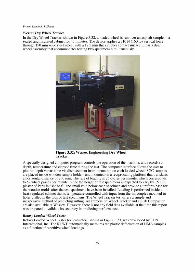
Brown, Kandhal, & Zhang
Wessex Dry Wheel Tracker
In the Dry Wheel Tracker, shown in Figure 3.32, a loaded wheel is run over an asphalt sample in a sealed and insulated cabinet for 45 minutes. The device applies a 710 N (160 lb) vertical force through 150 mm wide steel wheel with a 12.5 mm thick rubber contact surface. It has a dual wheel assembly that accommodates testing two specimens simultaneously.
Figure 3.32: Wessex Engineering Dry Wheel Tracker
A specially designed computer program controls the operation of the machine, and records rut
depth, temperature and elapsed time during the test. The computer interface allows the user to plot rut depth versus time via displacement instrumentation on each loaded wheel. SGC samples are placed inside wooden sample holders and mounted on a reciprocating platform that translates a horizontal distance of 230 mm. The rate of loading is 26 cycles per minute, which corresponds to 52 wheel passes per minute. Since the height of test specimens is expected to vary by ±5 mm, plaster of Paris is used to fill the small void below each specimen and provide a uniform base for the wooden molds after the test specimens have been installed. Loading is performed inside a heat-regulated cabinet that is temperature controlled with input from thermocouples mounted in holes drilled in the tops of test specimens. The Wheel Tracker test offers a simple and inexpensive method of predicting rutting. An Immersion Wheel Tracker and a Slab Compactor are also available at Wessex. However, there is not any field data available at the time this report was prepared to validate its accuracy in predicting performance.
Rotary Loaded Wheel Tester
Rotary Loaded Wheel Tester (or Rutmeter), shown in Figure 3.33, was developed by CPN International, Inc. The RLWT automatically measures the plastic deformation of HMA samples as a function of repetitive wheel loadings.
36
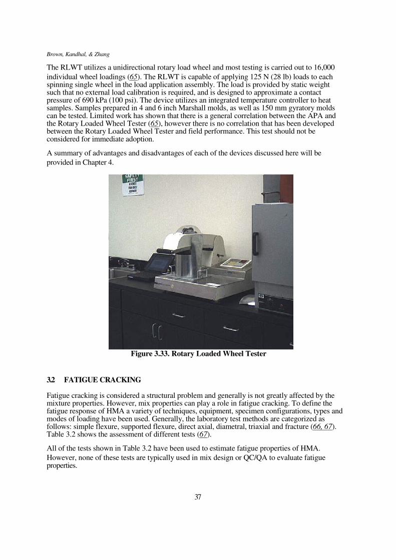
Brown, Kandhal, & Zhang
The RLWT utilizes a unidirectional rotary load wheel and most testing is carried out to 16,000
individual wheel loadings (65). The RLWT is capable of applying 125 N (28 lb) loads to each spinning single wheel in the load application assembly. The load is provided by static weight such that no external load calibration is required, and is designed to approximate a contact pressure of 690 kPa (100 psi). The device utilizes an integrated temperature controller to heat samples. Samples prepared in 4 and 6 inch Marshall molds, as well as 150 mm gyratory molds can be tested. Limited work has shown that there is a general correlation between the APA and the Rotary Loaded Wheel Tester (65), however there is no correlation that has been developed between the Rotary Loaded Wheel Tester and field performance. This test should not be considered for immediate adoption.
A summary of advantages and disadvantages of each of the devices discussed here will be
provided in Chapter 4.
Figure 3.33. Rotary Loaded Wheel Tester
3.2 FATIGUE CRACKING Fatigue cracking is considered a structural problem and generally is not greatly affected by the mixture properties. However, mix properties can play a role in fatigue cracking. To define the fatigue response of HMA a variety of techniques, equipment, specimen configurations, types and modes of loading have been used. Generally, the laboratory test methods are categorized as follows: simple flexure, supported flexure, direct axial, diametral, triaxial and fracture (66, 67). Table 3.2 shows the assessment of different tests (67).
All of the tests shown in Table 3.2 have been used to estimate fatigue properties of HMA.
However, none of these tests are typically used in mix design or QC/QA to evaluate fatigue properties.
37
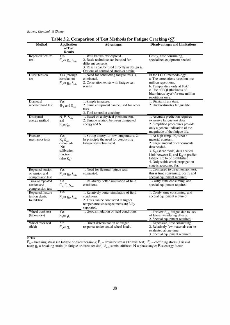
Brown, Kandhal, & Zhang
Table 3.2. Comparison of Test Methods for Fatigue Cracking (67) Method
Repeated flexure test
Direct tension test Diametral repeated load test
Dissipated energy method
Fracture mechanics tests Repeated tension or tension and compression test Triaxial repeated tension and compression test Repeated flexure test on elastic foundation
Wheel track test (laboratory) Wheel track test (field)
Application of Test Results
Yes Fb or gb, Smix
Yes (through correlation) Fb or gb, Smix
Yes 4Fb and Smix
N, R, Smix and Fb or gb,
Yes KI, Smix curve (a/h -N); calibration function (also KII)
Yes Fb or gb, Smix
Yes Fd, Fc, Smix
Yes Fb or gb, Smix
Yes F0 or gb
Yes Fb or gb
Advantages
1. Well known, widespread. 2. Basic technique can be used for different concepts 3. Results can be used directly in design 4. Options of controlled stress or strain. 1. Need for conducting fatigue tests is eliminated. 2. Correlation exists with fatigue test results.
1. Simple in nature. 2. Same equipment can be used for other tests. 3. Tool to predict cracking. 1. Based on a physical phenomenon. 2. Unique relation between dissipated energy and N.
1. Strong theory for low temperature. 2. In principle the need for conducting fatigue tests eliminated. 1. Need for flexural fatigue tests eliminated. 1. Relatively better simulation of field conditions. 1. Relatively better simulation of field conditions. 2. Tests can be conducted at higher temperature since specimens are fully supported. 1. Good simulation of field conditions.
1. Direct determination of fatigue response under actual wheel loads.
Disadvantages and Limitations
Costly, time consuming, specialized equipment needed.
In the LCPC methodology: a. The correlations based on one million repetitions. b. Temperature only at 10/C. c. Use of EQI (thickness of bituminous layer) for one million repetitions only. 1. Biaxial stress state. 2. Underestimates fatigue life.
1. Accurate prediction requires extensive fatigue test data. 2. Simplified procedures provide only a general indication of the magnitude of the fatigue life. 1. At high temp., KI is not a material constant. 2. Large amount of experimental data needed. 3. KII (shear mode) data needed. Link between KI and KII to predict fatigue life to be established. 4. Only stable crack propagation state is accounted for. 1. Compared to direct tension test, this is time consuming, costly and special equipment required. 1.Costly, time consuming, and special equipment required. 1. Costly, time consuming, and special equipment required.
1. For low Smix fatigue due to lack of lateral wandering effects. 2. Special equipment required. 1. Expensive, time consuming. 2. Relatively few materials can be evaluated at one time. 3. Special equipment required.
Notes: Fb = breaking stress (in fatigue or direct tension); Fd = deviator stress (Triaxial test); Fc = confining stress (Triaxial test); gb = breaking strain (in fatigue or direct tension); Smix = mix stiffness; N = phase angle; R = energy factor
38
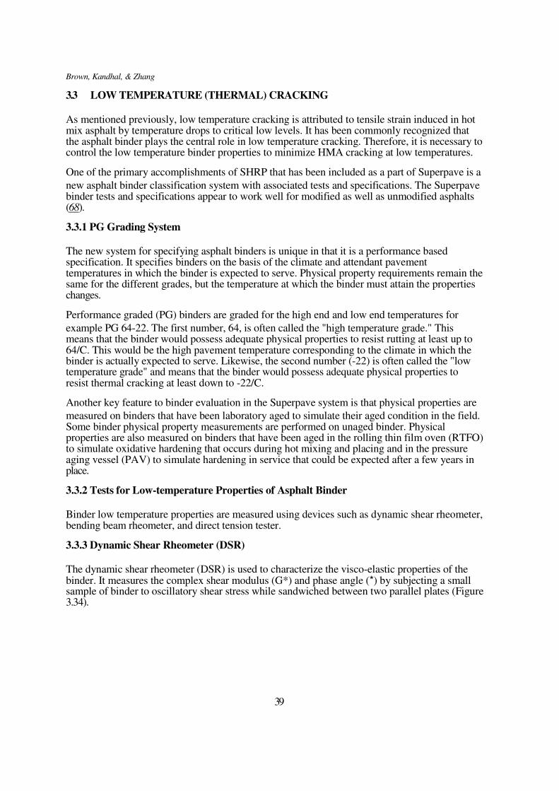
Brown, Kandhal, & Zhang
3.3 LOW TEMPERATURE (THERMAL) CRACKING
As mentioned previously, low temperature cracking is attributed to tensile strain induced in hot mix asphalt by temperature drops to critical low levels. It has been commonly recognized that the asphalt binder plays the central role in low temperature cracking. Therefore, it is necessary to control the low temperature binder properties to minimize HMA cracking at low temperatures.
One of the primary accomplishments of SHRP that has been included as a part of Superpave is a
new asphalt binder classification system with associated tests and specifications. The Superpave binder tests and specifications appear to work well for modified as well as unmodified asphalts (68).
3.3.1 PG Grading System
The new system for specifying asphalt binders is unique in that it is a performance based specification. It specifies binders on the basis of the climate and attendant pavement temperatures in which the binder is expected to serve. Physical property requirements remain the same for the different grades, but the temperature at which the binder must attain the properties changes.
Performance graded (PG) binders are graded for the high end and low end temperatures for
example PG 64-22. The first number, 64, is often called the "high temperature grade." This means that the binder would possess adequate physical properties to resist rutting at least up to 64/C. This would be the high pavement temperature corresponding to the climate in which the binder is actually expected to serve. Likewise, the second number (-22) is often called the "low temperature grade" and means that the binder would possess adequate physical properties to resist thermal cracking at least down to -22/C.
Another key feature to binder evaluation in the Superpave system is that physical properties are
measured on binders that have been laboratory aged to simulate their aged condition in the field. Some binder physical property measurements are performed on unaged binder. Physical properties are also measured on binders that have been aged in the rolling thin film oven (RTFO) to simulate oxidative hardening that occurs during hot mixing and placing and in the pressure aging vessel (PAV) to simulate hardening in service that could be expected after a few years in place.
3.3.2 Tests for Low-temperature Properties of Asphalt Binder
Binder low temperature properties are measured using devices such as dynamic shear rheometer, bending beam rheometer, and direct tension tester.
3.3.3 Dynamic Shear Rheometer (DSR)
The dynamic shear rheometer (DSR) is used to characterize the visco-elastic properties of the binder. It measures the complex shear modulus (G*) and phase angle (*) by subjecting a small sample of binder to oscillatory shear stress while sandwiched between two parallel plates (Figure 3.34).
39
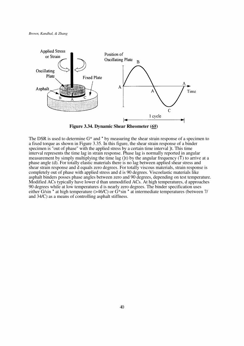
Brown, Kandhal, & Zhang
Figure 3.34. Dynamic Shear Rheometer (68)
The DSR is used to determine G* and * by measuring the shear strain response of a specimen to a fixed torque as shown in Figure 3.35. In this figure, the shear strain response of a binder specimen is "out of phase" with the applied stress by a certain time interval )t. This time interval represents the time lag in strain response. Phase lag is normally reported in angular measurement by simply multiplying the time lag ()t) by the angular frequency (T) to arrive at a phase angle (d). For totally elastic materials there is no lag between applied shear stress and shear strain response and d equals zero degrees. For totally viscous materials, strain response is completely out of phase with applied stress and d is 90 degrees. Viscoelastic materials like asphalt binders posses phase angles between zero and 90 degrees, depending on test temperature. Modified ACs typically have lower d than unmodified ACs. At high temperatures, d approaches 90 degrees while at low temperatures d is nearly zero degrees. The binder specification uses either G/sin * at high temperature (>46/C) or G*sin * at intermediate temperatures (between 7/ and 34/C) as a means of controlling asphalt stiffness.
40
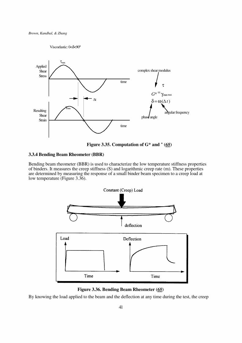
Brown, Kandhal, & Zhang
Viscoelastic: 0<δ<90°
τmax Applied
Shear Stress
time
complex shear modulus
τ
∆t
G* = γ max max
δ = ω (∆ t )
Resulting Shear Strain
γmax time
phase angle
angular frequency
Figure 3.35. Computation of G* and * (68)
3.3.4 Bending Beam Rheometer (BBR) Bending beam rheometer (BBR) is used to characterize the low temperature stiffness properties of binders. It measures the creep stiffness (S) and logarithmic creep rate (m). These properties are determined by measuring the response of a small binder beam specimen to a creep load at low temperature (Figure 3.36).
Figure 3.36. Bending Beam Rheometer (68)
By knowing the load applied to the beam and the deflection at any time during the test, the creep
41
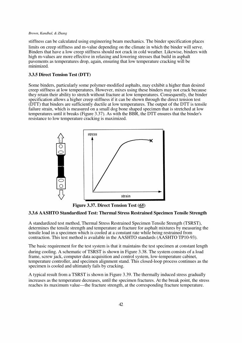
Brown, Kandhal, & Zhang
stiffness can be calculated using engineering beam mechanics. The binder specification places
limits on creep stiffness and m-value depending on the climate in which the binder will serve. Binders that have a low creep stiffness should not crack in cold weather. Likewise, binders with high m-values are more effective in relaxing and lowering stresses that build in asphalt pavements as temperatures drop, again, ensuring that low temperature cracking will be minimized.
3.3.5 Direct Tension Test (DTT)
Some binders, particularly some polymer-modified asphalts, may exhibit a higher than desired creep stiffness at low temperatures. However, mixes using these binders may not crack because they retain their ability to stretch without fracture at low temperatures. Consequently, the binder specification allows a higher creep stiffness if it can be shown through the direct tension test (DTT) that binders are sufficiently ductile at low temperatures. The output of the DTT is tensile failure strain, which is measured on a small dog bone shaped specimen that is stretched at low temperatures until it breaks (Figure 3.37). As with the BBR, the DTT ensures that the binder's resistance to low temperature cracking is maximized.
Figure 3.37. Direct Tension Test (68)
3.3.6 AASHTO Standardized Test: Thermal Stress Restrained Specimen Tensile Strength
A standardized test method, Thermal Stress Restrained Specimen Tensile Strength (TSRST), determines the tensile strength and temperature at fracture for asphalt mixtures by measuring the tensile load in a specimen which is cooled at a constant rate while being restrained from contraction. This test method is available in the AASHTO standards (AASHTO TP10-93).
The basic requirement for the test system is that it maintains the test specimen at constant length
during cooling. A schematic of TSRST is shown in Figure 3.38. The system consists of a load frame, screw jack, computer data acquisition and control system, low-temperature cabinet, temperature controller, and specimen alignment stand. This closed-loop process continues as the specimen is cooled and ultimately fails by cracking.
A typical result from a TSRST is shown in Figure 3.39. The thermally induced stress gradually
increases as the temperature decreases, until the specimen fractures. At the break point, the stress reaches its maximum value—the fracture strength, at the corresponding fracture temperature.
42
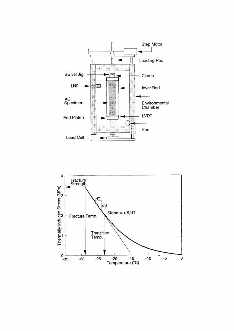

ERROR: stackunderflow
OFFENDING COMMAND: ~
STACK: