Embed Size (px)
Citation preview

Chapter 3 Numerical Characteristics and Characteristic Functions
3.2 Variances, Covariances and Correlation coefficients
3.4.1 Density functions and characteristic functions
3.4 Multivariate normal distributions
3.4.1 Density functions and characteristic functions
The pdf of n-dimensional normal distributionN(a, B) (B is positive definite symmetric matrix) :
p(x) =1
(2π)n/2|B|1/2exp{−1
2(x− a)′B−1(x− a)}.
Its c.f. is
f(t) = exp(it′a− 1
2t′Bt),
i.e.,
f(t1, · · · , tn) = exp(in∑
k=1
aktk −1
2
n∑l=1
n∑s=1
blstlts).

Chapter 3 Numerical Characteristics and Characteristic Functions
3.2 Variances, Covariances and Correlation coefficients
3.4.1 Density functions and characteristic functions
3.4 Multivariate normal distributions
3.4.1 Density functions and characteristic functionsThe pdf of n-dimensional normal distributionN(a, B) (B is positive definite symmetric matrix) :
p(x) =1
(2π)n/2|B|1/2exp{−1
2(x− a)′B−1(x− a)}.
Its c.f. is
f(t) = exp(it′a− 1
2t′Bt),
i.e.,
f(t1, · · · , tn) = exp(in∑
k=1
aktk −1
2
n∑l=1
n∑s=1
blstlts).

Chapter 3 Numerical Characteristics and Characteristic Functions
3.2 Variances, Covariances and Correlation coefficients
3.4.1 Density functions and characteristic functions
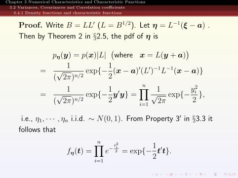
Proof. Write B = LL′ (L = B1/2). Let η = L−1(ξ − a) .
Then by Theorem 2 in §2.5, the pdf of η is
pη(y) = p(x)|L|(where x = L(y + a)
)
=1
(√2π)n/2
exp{−1
2(x− a)′(L′)−1L−1(x− a)}
=1
(√2π)n/2
exp{−1
2y′y} =
n∏i=1
1√2π
exp{−y2i
2},
i.e., η1, · · · , ηn i.i.d. ∼ N(0, 1). From Property 3′ in §3.3 it
follows that
fη(t) =n∏
i=1
e−t2i2 = exp{−1
2t′t}.

Chapter 3 Numerical Characteristics and Characteristic Functions
3.2 Variances, Covariances and Correlation coefficients
3.4.1 Density functions and characteristic functions
Proof. Write B = LL′ (L = B1/2). Let η = L−1(ξ − a) .
Then by Theorem 2 in §2.5, the pdf of η is
pη(y) = p(x)|L|(where x = L(y + a)
)=
1
(√2π)n/2
exp{−1
2(x− a)′(L′)−1L−1(x− a)}
=1
(√2π)n/2
exp{−1
2y′y} =
n∏i=1
1√2π
exp{−y2i
2},
i.e., η1, · · · , ηn i.i.d. ∼ N(0, 1). From Property 3′ in §3.3 it
follows that
fη(t) =n∏
i=1
e−t2i2 = exp{−1
2t′t}.
Chapter 3 Numerical Characteristics and Characteristic Functions
3.2 Variances, Covariances and Correlation coefficients
3.4.1 Density functions and characteristic functions
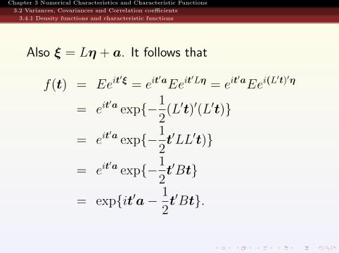
Also ξ = Lη + a. It follows that
f(t) = Eeit′ξ = eit
′aEeit′Lη = eit
′aEei(L′t)′η
= eit′a exp{−1
2(L′t)′(L′t)}
= eit′a exp{−1
2t′LL′t)}
= eit′a exp{−1
2t′Bt}
= exp{it′a− 1
2t′Bt}.

Chapter 3 Numerical Characteristics and Characteristic Functions
3.2 Variances, Covariances and Correlation coefficients
3.4.1 Density functions and characteristic functions
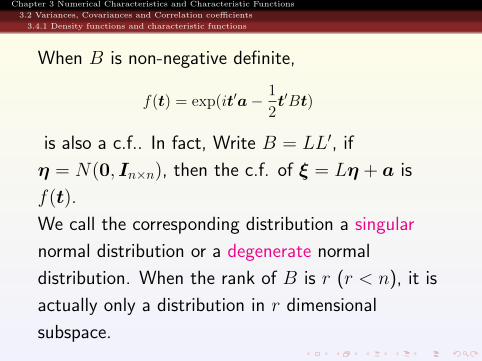
When B is non-negative definite,
f(t) = exp(it′a− 1
2t′Bt)
is also a c.f.. In fact, Write B = LL′, if
η = N(0, In×n), then the c.f. of ξ = Lη + a is
f(t).
We call the corresponding distribution a singular
normal distribution or a degenerate normal
distribution. When the rank of B is r (r < n), it is
actually only a distribution in r dimensional
subspace.
Chapter 3 Numerical Characteristics and Characteristic Functions
3.2 Variances, Covariances and Correlation coefficients
3.4.1 Density functions and characteristic functions
When B is non-negative definite,
f(t) = exp(it′a− 1
2t′Bt)
is also a c.f.. In fact, Write B = LL′, if
η = N(0, In×n), then the c.f. of ξ = Lη + a is
f(t).
We call the corresponding distribution a singular
normal distribution or a degenerate normal
distribution. When the rank of B is r (r < n), it is
actually only a distribution in r dimensional
subspace.

Chapter 3 Numerical Characteristics and Characteristic Functions
3.2 Variances, Covariances and Correlation coefficients
3.4.2 Properties
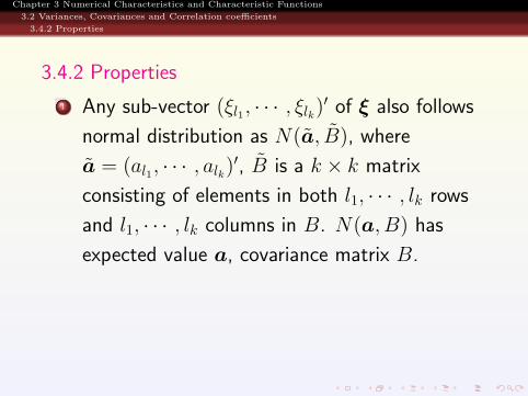
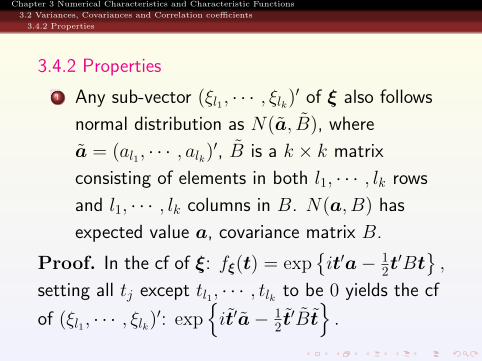
3.4.2 Properties
1 Any sub-vector (ξl1, · · · , ξlk)′ of ξ also follows
normal distribution as N(a, B), where
a = (al1, · · · , alk)′, B is a k × k matrix
consisting of elements in both l1, · · · , lk rows
and l1, · · · , lk columns in B. N(a, B) has
expected value a, covariance matrix B.
Proof. In the cf of ξ: fξ(t) = exp{it′a− 1
2t′Bt},
setting all tj except tl1, · · · , tlk to be 0 yields the cf
of (ξl1, · · · , ξlk)′: exp{it′a− 1
2 t′Bt}.
Chapter 3 Numerical Characteristics and Characteristic Functions
3.2 Variances, Covariances and Correlation coefficients
3.4.2 Properties
3.4.2 Properties
1 Any sub-vector (ξl1, · · · , ξlk)′ of ξ also follows
normal distribution as N(a, B), where
a = (al1, · · · , alk)′, B is a k × k matrix
consisting of elements in both l1, · · · , lk rows
and l1, · · · , lk columns in B. N(a, B) has
expected value a, covariance matrix B.
Proof. In the cf of ξ: fξ(t) = exp{it′a− 1
2t′Bt},
setting all tj except tl1, · · · , tlk to be 0 yields the cf
of (ξl1, · · · , ξlk)′: exp{it′a− 1
2 t′Bt}.
Chapter 3 Numerical Characteristics and Characteristic Functions
3.2 Variances, Covariances and Correlation coefficients
3.4.2 Properties
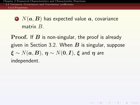
2 N(a,B) has expected value a, covariance
matrix B.
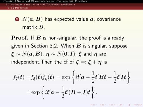
Proof. If B is non-singular, the proof is already
given in Section 3.2. When B is singular, suppose
ξ ∼ N(a,B), η ∼ N(0, I), ξ and η are
independent.Then the cf of ζ =: ξ + η is
fζ(t) =fξ(t)fη(t) = exp
{it′a− 1
2t′Bt− 1
2t′It
}=exp
{it′a− 1
2t′(B + I)t
}.

Chapter 3 Numerical Characteristics and Characteristic Functions
3.2 Variances, Covariances and Correlation coefficients
3.4.2 Properties
2 N(a,B) has expected value a, covariance
matrix B.
Proof. If B is non-singular, the proof is already
given in Section 3.2. When B is singular, suppose
ξ ∼ N(a,B), η ∼ N(0, I), ξ and η are
independent.Then the cf of ζ =: ξ + η is
fζ(t) =fξ(t)fη(t) = exp
{it′a− 1
2t′Bt− 1
2t′It
}=exp
{it′a− 1
2t′(B + I)t
}.
Chapter 3 Numerical Characteristics and Characteristic Functions
3.2 Variances, Covariances and Correlation coefficients
3.4.2 Properties
2 N(a,B) has expected value a, covariance
matrix B.
Proof. If B is non-singular, the proof is already
given in Section 3.2. When B is singular, suppose
ξ ∼ N(a,B), η ∼ N(0, I), ξ and η are
independent.
Then the cf of ζ =: ξ + η is
fζ(t) =fξ(t)fη(t) = exp
{it′a− 1
2t′Bt− 1
2t′It
}=exp
{it′a− 1
2t′(B + I)t
}.
Chapter 3 Numerical Characteristics and Characteristic Functions
3.2 Variances, Covariances and Correlation coefficients
3.4.2 Properties
2 N(a,B) has expected value a, covariance
matrix B.
Proof. If B is non-singular, the proof is already
given in Section 3.2. When B is singular, suppose
ξ ∼ N(a,B), η ∼ N(0, I), ξ and η are
independent.Then the cf of ζ =: ξ + η is
fζ(t) =fξ(t)fη(t) = exp
{it′a− 1
2t′Bt− 1
2t′It
}=exp
{it′a− 1
2t′(B + I)t
}.

Chapter 3 Numerical Characteristics and Characteristic Functions
3.2 Variances, Covariances and Correlation coefficients
3.4.2 Properties
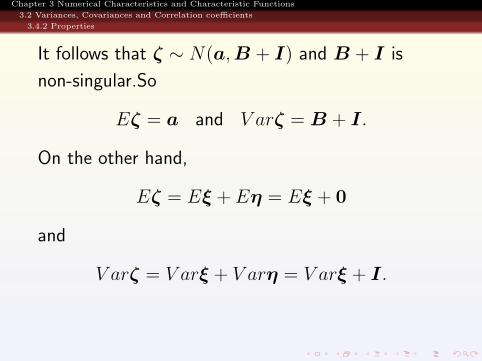
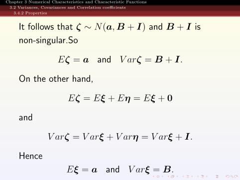
It follows that ζ ∼ N(a,B + I) and B + I is
non-singular.
So
Eζ = a and V arζ = B + I.
On the other hand,
Eζ = Eξ + Eη = Eξ + 0
and
V arζ = V arξ + V arη = V arξ + I.
Hence
Eξ = a and V arξ = B.

Chapter 3 Numerical Characteristics and Characteristic Functions
3.2 Variances, Covariances and Correlation coefficients
3.4.2 Properties
It follows that ζ ∼ N(a,B + I) and B + I is
non-singular.So
Eζ = a and V arζ = B + I.
On the other hand,
Eζ = Eξ + Eη = Eξ + 0
and
V arζ = V arξ + V arη = V arξ + I.
Hence
Eξ = a and V arξ = B.

Chapter 3 Numerical Characteristics and Characteristic Functions
3.2 Variances, Covariances and Correlation coefficients
3.4.2 Properties
3 ξ1, · · · , ξn with joint normal distribution are
mutually independent iff they are pairwise
uncorrelated. (Proof. Omitted.)

Chapter 3 Numerical Characteristics and Characteristic Functions
3.2 Variances, Covariances and Correlation coefficients
3.4.2 Properties
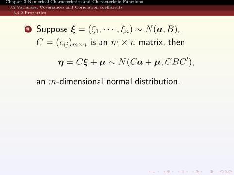
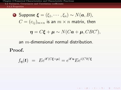
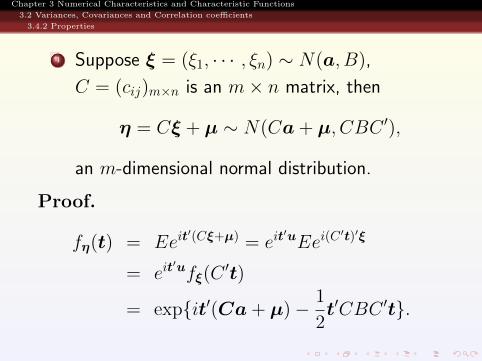
4 Suppose ξ = (ξ1, · · · , ξn) ∼ N(a, B),
C = (cij)m×n is an m× n matrix, then
η = Cξ + µ ∼ N(Ca+ µ, CBC ′),
an m-dimensional normal distribution.
Proof.
fη(t) = Eeit′(Cξ+µ) = eit
′uEei(C′t)′ξ
= eit′ufξ(C
′t)
= exp{it′(Ca+ µ)− 1
2t′CBC ′t}.
Chapter 3 Numerical Characteristics and Characteristic Functions
3.2 Variances, Covariances and Correlation coefficients
3.4.2 Properties
4 Suppose ξ = (ξ1, · · · , ξn) ∼ N(a, B),
C = (cij)m×n is an m× n matrix, then
η = Cξ + µ ∼ N(Ca+ µ, CBC ′),
an m-dimensional normal distribution.
Proof.
fη(t) = Eeit′(Cξ+µ) = eit
′uEei(C′t)′ξ
= eit′ufξ(C
′t)
= exp{it′(Ca+ µ)− 1
2t′CBC ′t}.
Chapter 3 Numerical Characteristics and Characteristic Functions
3.2 Variances, Covariances and Correlation coefficients
3.4.2 Properties
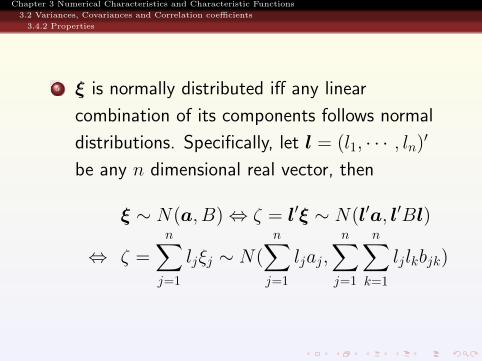
5 ξ is normally distributed iff any linear
combination of its components follows normal
distributions. Specifically, let l = (l1, · · · , ln)′
be any n dimensional real vector, then
ξ ∼ N(a, B)⇔ ζ = l′ξ ∼ N(l′a, l′Bl)
⇔ ζ =n∑j=1
ljξj ∼ N(n∑j=1
ljaj,n∑j=1
n∑k=1
ljlkbjk)
Chapter 3 Numerical Characteristics and Characteristic Functions
3.2 Variances, Covariances and Correlation coefficients
3.4.2 Properties
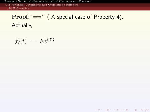
Proof.”=⇒” ( A special case of Property 4).
Actually,
fζ(t) = Eeitl′ξ
= exp
{i(tl)′a− 1
2(tl)′)B(tl)
}= exp
{it(l′a)− 1
2t2l′Bl
}.
So ζ = l′ξ ∼ N(l′a, l′Bl).
”⇐=” First, by assumption, each ξk is normal. So
its mean and variance exists, and then Cov{ξk, ξj}exists. Denote a = Eξ and B = V arξ. We want
to show that ξ ∼ N(a, B).

Chapter 3 Numerical Characteristics and Characteristic Functions
3.2 Variances, Covariances and Correlation coefficients
3.4.2 Properties
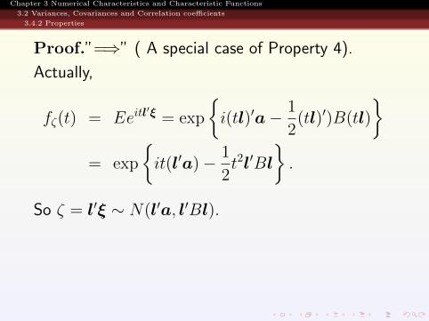
Proof.”=⇒” ( A special case of Property 4).
Actually,
fζ(t) = Eeitl′ξ = exp
{i(tl)′a− 1
2(tl)′)B(tl)
}= exp
{it(l′a)− 1
2t2l′Bl
}.
So ζ = l′ξ ∼ N(l′a, l′Bl).
”⇐=” First, by assumption, each ξk is normal. So
its mean and variance exists, and then Cov{ξk, ξj}exists. Denote a = Eξ and B = V arξ. We want
to show that ξ ∼ N(a, B).
Chapter 3 Numerical Characteristics and Characteristic Functions
3.2 Variances, Covariances and Correlation coefficients
3.4.2 Properties
Proof.”=⇒” ( A special case of Property 4).
Actually,
fζ(t) = Eeitl′ξ = exp
{i(tl)′a− 1
2(tl)′)B(tl)
}= exp
{it(l′a)− 1
2t2l′Bl
}.
So ζ = l′ξ ∼ N(l′a, l′Bl).
”⇐=” First, by assumption, each ξk is normal. So
its mean and variance exists, and then Cov{ξk, ξj}exists. Denote a = Eξ and B = V arξ. We want
to show that ξ ∼ N(a, B).

Chapter 3 Numerical Characteristics and Characteristic Functions
3.2 Variances, Covariances and Correlation coefficients
3.4.2 Properties
Proof.”=⇒” ( A special case of Property 4).
Actually,
fζ(t) = Eeitl′ξ = exp
{i(tl)′a− 1
2(tl)′)B(tl)
}= exp
{it(l′a)− 1
2t2l′Bl
}.
So ζ = l′ξ ∼ N(l′a, l′Bl).
”⇐=” First, by assumption, each ξk is normal. So
its mean and variance exists, and then Cov{ξk, ξj}exists.
Denote a = Eξ and B = V arξ. We want
to show that ξ ∼ N(a, B).

Chapter 3 Numerical Characteristics and Characteristic Functions
3.2 Variances, Covariances and Correlation coefficients
3.4.2 Properties
Proof.”=⇒” ( A special case of Property 4).
Actually,
fζ(t) = Eeitl′ξ = exp
{i(tl)′a− 1
2(tl)′)B(tl)
}= exp
{it(l′a)− 1
2t2l′Bl
}.
So ζ = l′ξ ∼ N(l′a, l′Bl).
”⇐=” First, by assumption, each ξk is normal. So
its mean and variance exists, and then Cov{ξk, ξj}exists. Denote a = Eξ and B = V arξ. We want
to show that ξ ∼ N(a, B).

Chapter 3 Numerical Characteristics and Characteristic Functions
3.2 Variances, Covariances and Correlation coefficients
3.4.2 Properties
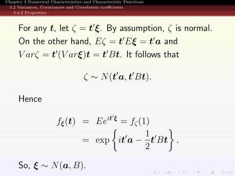
For any t, let ζ = t′ξ. By assumption, ζ is normal.
On the other hand, Eζ = t′Eξ = t′a and
V arζ = t′(V arξ)t = t′Bt. It follows that
ζ ∼ N(t′a, t′Bt).
Hence
fξ(t) = Eeit′ξ = fζ(1)
= exp
{it′a− 1
2t′Bt
}.
So, ξ ∼ N(a, B).

Chapter 3 Numerical Characteristics and Characteristic Functions
3.2 Variances, Covariances and Correlation coefficients
3.4.2 Properties
For any t, let ζ = t′ξ. By assumption, ζ is normal.
On the other hand, Eζ = t′Eξ = t′a and
V arζ = t′(V arξ)t = t′Bt.
It follows that
ζ ∼ N(t′a, t′Bt).
Hence
fξ(t) = Eeit′ξ = fζ(1)
= exp
{it′a− 1
2t′Bt
}.
So, ξ ∼ N(a, B).

Chapter 3 Numerical Characteristics and Characteristic Functions
3.2 Variances, Covariances and Correlation coefficients
3.4.2 Properties
For any t, let ζ = t′ξ. By assumption, ζ is normal.
On the other hand, Eζ = t′Eξ = t′a and
V arζ = t′(V arξ)t = t′Bt. It follows that
ζ ∼ N(t′a, t′Bt).
Hence
fξ(t) = Eeit′ξ = fζ(1)
= exp
{it′a− 1
2t′Bt
}.
So, ξ ∼ N(a, B).
Chapter 3 Numerical Characteristics and Characteristic Functions
3.2 Variances, Covariances and Correlation coefficients
3.4.2 Properties
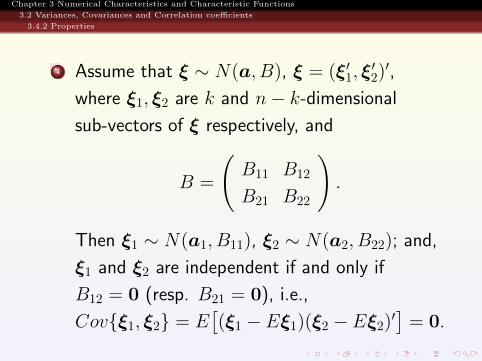
4 Assume that ξ ∼ N(a, B), ξ = (ξ′1, ξ′2)′,
where ξ1, ξ2 are k and n− k-dimensional
sub-vectors of ξ respectively, and
B =
(B11 B12
B21 B22
).
Then ξ1 ∼ N(a1, B11), ξ2 ∼ N(a2, B22); and,
ξ1 and ξ2 are independent if and only if
B12 = 0 (resp. B21 = 0), i.e.,
Cov{ξ1, ξ2} = E[(ξ1 − Eξ1)(ξ2 − Eξ2)′
]= 0.
Chapter 3 Numerical Characteristics and Characteristic Functions
3.2 Variances, Covariances and Correlation coefficients
3.4.2 Properties
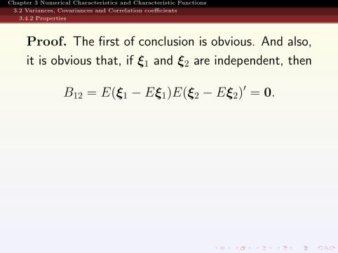
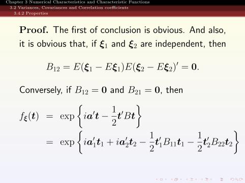
Proof. The first of conclusion is obvious. And also,
it is obvious that, if ξ1 and ξ2 are independent, then
B12 = E(ξ1 − Eξ1)E(ξ2 − Eξ2)′ = 0.
Conversely, if B12 = 0 and B21 = 0, then
fξ(t) = exp
{ia′t− 1
2t′Bt
}= exp
{ia′1t1 + ia′2t2 −
1
2t′1B11t1 −
1
2t′2B22t2
}= fξ1(t1)fξ2(t2).

Chapter 3 Numerical Characteristics and Characteristic Functions
3.2 Variances, Covariances and Correlation coefficients
3.4.2 Properties
Proof. The first of conclusion is obvious. And also,
it is obvious that, if ξ1 and ξ2 are independent, then
B12 = E(ξ1 − Eξ1)E(ξ2 − Eξ2)′ = 0.
Conversely, if B12 = 0 and B21 = 0, then
fξ(t) = exp
{ia′t− 1
2t′Bt
}
= exp
{ia′1t1 + ia′2t2 −
1
2t′1B11t1 −
1
2t′2B22t2
}= fξ1(t1)fξ2(t2).
Chapter 3 Numerical Characteristics and Characteristic Functions
3.2 Variances, Covariances and Correlation coefficients
3.4.2 Properties
Proof. The first of conclusion is obvious. And also,
it is obvious that, if ξ1 and ξ2 are independent, then
B12 = E(ξ1 − Eξ1)E(ξ2 − Eξ2)′ = 0.
Conversely, if B12 = 0 and B21 = 0, then
fξ(t) = exp
{ia′t− 1
2t′Bt
}= exp
{ia′1t1 + ia′2t2 −
1
2t′1B11t1 −
1
2t′2B22t2
}
= fξ1(t1)fξ2(t2).

Chapter 3 Numerical Characteristics and Characteristic Functions
3.2 Variances, Covariances and Correlation coefficients
3.4.2 Properties
Proof. The first of conclusion is obvious. And also,
it is obvious that, if ξ1 and ξ2 are independent, then
B12 = E(ξ1 − Eξ1)E(ξ2 − Eξ2)′ = 0.
Conversely, if B12 = 0 and B21 = 0, then
fξ(t) = exp
{ia′t− 1
2t′Bt
}= exp
{ia′1t1 + ia′2t2 −
1
2t′1B11t1 −
1
2t′2B22t2
}= fξ1(t1)fξ2(t2).
Chapter 3 Numerical Characteristics and Characteristic Functions
3.2 Variances, Covariances and Correlation coefficients
3.4.2 Properties
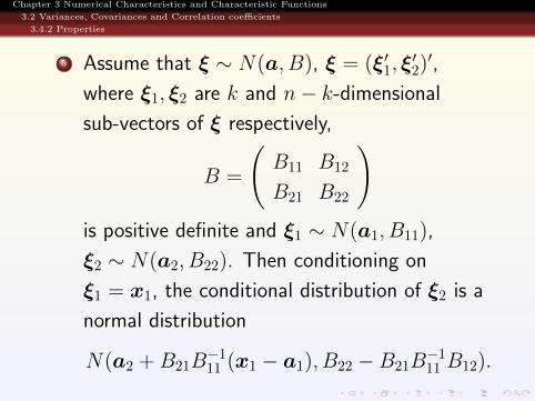
5 Assume that ξ ∼ N(a, B), ξ = (ξ′1, ξ′2)′,
where ξ1, ξ2 are k and n− k-dimensional
sub-vectors of ξ respectively,
B =
(B11 B12
B21 B22
)is positive definite and ξ1 ∼ N(a1, B11),
ξ2 ∼ N(a2, B22). Then conditioning on
ξ1 = x1, the conditional distribution of ξ2 is a
normal distribution
N(a2 +B21B−111 (x1 − a1), B22 −B21B
−111 B12).
Chapter 3 Numerical Characteristics and Characteristic Functions
3.2 Variances, Covariances and Correlation coefficients
3.4.2 Properties
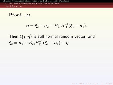
Proof. Let
η = ξ2 − a2 −B21B−111 (ξ1 − a1).
Then (ξ1,η) is still normal random vector, and
ξ2 = a2 +B21B−111 (ξ1 − a1) + η.
It is easily seen
that Eη = 0 and
V arη =B22 − 2B21B−111 B12 +B21B
−111 B11(B21B
−111 )′
=B22 −B21B−111 B12=Σ.
It follows that η ∼ N(0,Σ).
Chapter 3 Numerical Characteristics and Characteristic Functions
3.2 Variances, Covariances and Correlation coefficients
3.4.2 Properties
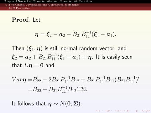
Proof. Let
η = ξ2 − a2 −B21B−111 (ξ1 − a1).
Then (ξ1,η) is still normal random vector, and
ξ2 = a2 +B21B−111 (ξ1 − a1) + η. It is easily seen
that Eη = 0 and
V arη =B22 − 2B21B−111 B12 +B21B
−111 B11(B21B
−111 )′
=B22 −B21B−111 B12=Σ.
It follows that η ∼ N(0,Σ).

Chapter 3 Numerical Characteristics and Characteristic Functions
3.2 Variances, Covariances and Correlation coefficients
3.4.2 Properties
Also,
Eη(ξ1 − a1)′ = B21 −B21B
−111 B11 = 0.
It follows that ξ1 and η are independent.
η∣∣ξ1=x1
∼ N(0,Σ).
It follows that
ξ2∣∣ξ1=x1
=a2 +B21B−111 (x1 − a1) + η
∣∣ξ1=x1
∼N(a2 +B21B−111 (x1 − a1),Σ).
Chapter 3 Numerical Characteristics and Characteristic Functions
3.2 Variances, Covariances and Correlation coefficients
3.4.2 Properties
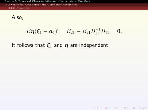
Also,
Eη(ξ1 − a1)′ = B21 −B21B
−111 B11 = 0.
It follows that ξ1 and η are independent.
η∣∣ξ1=x1
∼ N(0,Σ).
It follows that
ξ2∣∣ξ1=x1
=a2 +B21B−111 (x1 − a1) + η
∣∣ξ1=x1
∼N(a2 +B21B−111 (x1 − a1),Σ).

Chapter 3 Numerical Characteristics and Characteristic Functions
3.2 Variances, Covariances and Correlation coefficients
3.4.2 Properties
Example
Suppose ξ1, . . . , ξn be i.i.d. normal N(µ, σ2)
random variables. Let
ξ =
∑nk=1 ξkn
, σ2 =1
n
n∑k=1
(ξk − ξ)2.
Show that ξ and σ2 are independent.
Chapter 3 Numerical Characteristics and Characteristic Functions
3.2 Variances, Covariances and Correlation coefficients
3.4.2 Properties
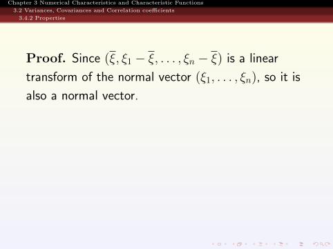
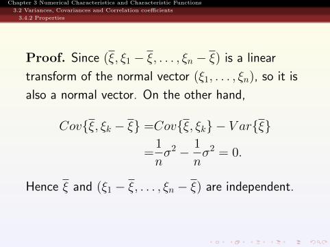
Proof. Since (ξ, ξ1 − ξ, . . . , ξn − ξ) is a linear
transform of the normal vector (ξ1, . . . , ξn), so it is
also a normal vector.
On the other hand,
Cov{ξ, ξk − ξ} =Cov{ξ, ξk} − V ar{ξ}
=1
nσ2 − 1
nσ2 = 0.
Hence ξ and (ξ1 − ξ, . . . , ξn − ξ) are independent.
So ξ and σ2 are independent.

Chapter 3 Numerical Characteristics and Characteristic Functions
3.2 Variances, Covariances and Correlation coefficients
3.4.2 Properties
Proof. Since (ξ, ξ1 − ξ, . . . , ξn − ξ) is a linear
transform of the normal vector (ξ1, . . . , ξn), so it is
also a normal vector. On the other hand,
Cov{ξ, ξk − ξ} =Cov{ξ, ξk} − V ar{ξ}
=1
nσ2 − 1
nσ2 = 0.
Hence ξ and (ξ1 − ξ, . . . , ξn − ξ) are independent.
So ξ and σ2 are independent.

Chapter 3 Numerical Characteristics and Characteristic Functions
3.2 Variances, Covariances and Correlation coefficients
3.4.2 Properties
Example 1. Assume
ξ = (ξ1, ξ2)′ ∼ N(a1, a2, σ
2, σ2, r), prove
η1 = ξ1 + ξ2 and η2 = ξ1 − ξ2 are independent, and
find respective distributions of η1, η2.
Chapter 3 Numerical Characteristics and Characteristic Functions
3.2 Variances, Covariances and Correlation coefficients
3.4.2 Properties
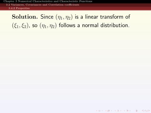
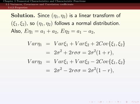
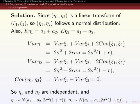
Solution. Since (η1, η2) is a linear transform of
(ξ1, ξ2), so (η1, η2) follows a normal distribution.
Also, Eη1 = a1 + a2, Eη2 = a1 − a2,
V arη1 = V arξ1 + V arξ2 + 2Cov{ξ1, ξ2}= 2σ2 + 2rσσ = 2σ2(1 + r),
V arη2 = V arξ1 + V arξ2 − 2Cov{ξ1, ξ2}= 2σ2 − 2rσσ = 2σ2(1− r),
Cov{η1, η2} = V arξ1 − V arξ2 = 0.
So η1 and η2 are independent, and
η1 ∼ N(a1 + a2, 2σ2(1 + r)), η2 ∼ N(a1 − a2, 2σ2(1− r)).

Chapter 3 Numerical Characteristics and Characteristic Functions
3.2 Variances, Covariances and Correlation coefficients
3.4.2 Properties
Solution. Since (η1, η2) is a linear transform of
(ξ1, ξ2), so (η1, η2) follows a normal distribution.
Also, Eη1 = a1 + a2, Eη2 = a1 − a2,
V arη1 = V arξ1 + V arξ2 + 2Cov{ξ1, ξ2}= 2σ2 + 2rσσ = 2σ2(1 + r),
V arη2 = V arξ1 + V arξ2 − 2Cov{ξ1, ξ2}= 2σ2 − 2rσσ = 2σ2(1− r),
Cov{η1, η2} = V arξ1 − V arξ2 = 0.
So η1 and η2 are independent, and
η1 ∼ N(a1 + a2, 2σ2(1 + r)), η2 ∼ N(a1 − a2, 2σ2(1− r)).