34. COMPARISON OF VELOCITIES DETERMINED FROM SONOBUOY, VSP

Gradstein, F. M., Ludden, J. N., et al., 1992Proceedings of the Ocean Drilling Program, Scientific Results, Vol. 123

34. COMPARISON OF VELOCITIES DETERMINED FROM SONOBUOY, VSP, CORE-SAMPLE,AND SONIC-LOG DATA FROM SITE 7651

D. Lizarralde2 and R. T. Buffler3

ABSTRACT

Several types of data were collected at Site 765 that can be used to determine the seismic velocities of the sediments.These data include a Sonobuoy profile, a vertical seismic profile, a sonic log, and traveltime measurements through coresamples. This study compares the velocity information determined from these various data sets, with emphasis on theanalyses of the Sonobuoy data. The Sonobuoy data were processed and analysed in the x-p domain to produce aninterval-velocity/depth profile. A comparison of the Sonobuoy results with the results of analyses of the other data setsreveals a good agreement among all of the velocity measurements. The velocity/depth profile determined from the analysesof the Sonobuoy data is used to convert normal-incidence reflection times to depth, thus enabling the lithologies observedin the cores from Site 765 to be tied to regional reflection profiles.

INTRODUCTION

The physical property of seismic velocity refers to the speedat which seismic energy propagates through a given medium. Theaccurate determination of the seismic velocities of various unitswithin a sedimentary column is essential to the task of convertingto depth the two-way, vertical traveltime of a reflection eventobserved on a seismic reflection profile. This time-to-depth con-version is especially important if the lithologies observed in coresdrilled from the ocean floor are to be extrapolated regionally usingregional reflection profiles.

We have analyzed Sonobuoy wide-angle-reflection data col-lected during Leg 123 of the Ocean Drilling Program (ODP) nearSite 765 on the Argo abyssal plain. The analysis involves thefitting of ellipses to the x-p transformed seismic data to determineinterval velocities. The results of the x-p analyses are comparedwith results from the more traditional approach of fitting hyper-bolas to the X-T data to determine RMS (root-mean-square) ve-locities and obtaining interval velocities from Dix's (1955) equation.

The velocity structure determined from the analyses of theSonobuoy data is compared with velocity information obtainedfrom other types of traveltime data collected at Site 765, including(1) traveltime measurements through core samples taken on boardthe JOIDES Resolution, (2) traveltime measurements from the seasurface to various depths within the borehole obtained during theVSP (vertical seismic profile) experiment, and (3) sonic logmeasurements, or traveltimes along the borehole over distancesof several meters.

Data Acquisition and AnalysesSonobuoy Line 2 (SB Line 2) (Fig. 1) extends from 5.5 km

northeast to 8.0 km southwest of Site 765, with the point of closestapproach located -1.5 km southeast of the site. During the dataacquisition the ship was traveling at a speed of approximately 7.5kt, and shots were fired every 20 s from two 80-in.3 water guns.

15 50S,

1 Gradstein, F. M., Ludden, J. N., et al., 1992. Proc. ODP, Sri. Results, 123:College Station, TX (Ocean Drilling Program).

2 Woods Hole Oceanographic Institute, Woods Hole, MA 02543, U.S.A.Institute for Geophysics, 8701 Mopac Boulevard, Austin, TX 78759-8375, U.S.A.

SB Line 2

10 km

117°40

Figure 1. Ship tracks of Sonobuoy Line 2 and BMR Rig Seismic Lines56-22 and 56-23C. The location of Site 765 is indicated.

The filter settings of the recording instruments were changed froma pass band of 5-250 Hz to 5-60 Hz after the 45th shot (-4.5 kmrange). The effect of the change in acquisition parameters isclearly seen in a reduced-time plot (T = T- X/1.5, Δ X = 99.0 m)of the direct-wave arrival (arrow, Fig. 2).

The SB Line 2 seismic profile is shown in Figure 3 out to arange of just beyond 13.0 km. The data have been band-passfiltered (5-55 Hz, zero-phase, Butterworth filter) and normalizedso that the maximum amplitude of each trace is one. The acquisi-tion-related change in trace character is again evident at -4.5 kmrange. However, with the exception of this one flaw, the qualityof the data is good.

625

D. LIZARRALDE, R. T. BUFFLER

70 60 50 40 30 20 10

Figure 2. Reduced-time plot of the direct-wave arrival: T = T- X/l.5, AX = 0.099 km. Arrow denotes change in acquisition filters from 5-250 Hz to5-60 Hz.

SONOBUOY DATA ANALYSES

x-p analyses

The x-p analyses of the Sonobuoy data involved (1) the trans-formation of the Sonobuoy data into the x-p domain and (2) theuse of the x-p normal-moveout technique to determine intervalvelocities from visually fit elliptical trajectories through the x-psection. Various aspects of the X-T to x-p transformation havebeen discussed in detail by McMechan and Ottolini (1980), Phin-ney et al. (1981), Stoffa et al. (1981), and others. The determina-tion of interval velocities by means of the x-p normal-moveoutmethod has been presented by Schultz (1982) and Stoffa et al.(1982). Theoretical aspects of the inversion problem thus will bediscussed only briefly here.

The sediments in the vicinity of Site 765 are, in general,horizontally stratified. Thus, we may assume that the velocitystructure of the sediments consists of a stack of homogeneous,laterally isotropic layers having thicknesses Z, and slownesses Mj= 1/Vj. If we consider a seismic ray path through this stack, thenthe vertical and horizontal components of slowness along the pathare given by

qj = Uj cos ij and pj = Uj sin ii•.= p, (1)

where ij is the angle of the ray in the yth layer with respect to thevertical and the horizontal component of slowness, or ray para-meter, p, remains constant along the ray path by SnelFs law. Thetotal traveltime for a plane wave reflected or refracted from thenth interface is then

(2)

where X is the offset distance between the source and the receiver.Equation 2 defines a straight line in the X-T domain that is

tangent to the traveltime curve at point (X,T), with slope p andintercept time

(3)/ = ]

The intercept time, T, is physically interpreted as the two-way,vertical traveltime of the ray with parameterp. The X-T traveltimecurves can be reparameterized in terms of x and p. For reflectionsfrom the base of a single, horizontal layer, we have

(4)

This equation describes an ellipse in the x-p plane. The x-pmappings of the X-T traveltime curves for multiple layers are thesums of ellipses (Schultz, 1976; Deibold and Stoffa, 1981)

(5)

The reflection from the first interface is a true ellipse in x-p,and the reflections from successively deeper interfaces havepseudo-elliptical trajectories.

The X-T to x-p MappingAn offset seismic section can be mapped into the x-p domain

by means of the slant stack. The term slant stack refers to theoperation of a constant-ray-parameter stack, or summation, alonglinear trajectories through an X-T seismic section at various inter-cept times. By slant stacking over a range of ray parameters, p,and intercept times, t, the entire X-T seismic section can bemapped into the x-p domain. This transformation is described bythe equation,

(6)

where / is the seismic section, F the x-p mapping, and N thenumber of X-T traces over which the summation is performed.

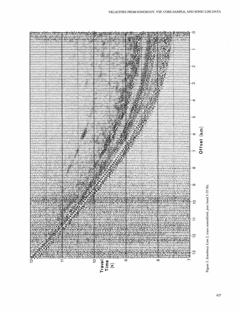
Unfortunately, the slant-stack process will introduce artifactsinto the x-p section if the X-T data are spatially aliased. A tracespacing less than one-half of the wavelength of the highest fre-quency one wishes to resolve is required to avoid spatial aliasing.The highest frequencies that we consider are 55 Hz, and thehorizontal phase velocities observed on the profile beyond 5 kmrange are between 2.0 and 3.0 km/s. To prevent spatial aliasing,the trace spacing would have to be 1/2 (2 km/s ÷ 55 Hz), or 18 m.The trace spacing of SB Line 2 is 99 m. Thus, the Sonobuoy dataare spatially aliased. Figure 4 shows the x-p section resulting froma standard slant stack of the Sonobuoy data in which all of thetraces of the profile were considered in each ray parameter stack.The elliptical trajectories of the reflection events are buried inaliased energy, which appears as linear events fanning out fromhigh to low values of p.

A number of windowing and interpolation schemes have beenproposed to reduce the problems associated with slant stackingspatially aliased, offset-seismic data (Schultz and Claerbout,1978; Stoffa et al., 1981; Singh et al., 1989). We use an approachthat incorporates a priori knowledge of the water depth, alongwith the thickness and average velocity of the sediments at Site765. With this information one can determine a range of ray

626

VELOCITIES FROM SONOBUOY, VSP, CORE-SAMPLE, AND SONIC-LOG DATA

Φ

627


P (s/km)

0.

5

6

Tαu(s)

iài

II

.1 .2

HMHBff i

öfclHipSliiII(i l l

.3

111 1 lil

• l i •llilli•si s i rIIJI Hill Illiilillll ;

.4

III 1 111 I SIB111 1 111 IJIH

MNPis lifii i1111 ^ W1 1 ;i

.5

mm

iIfI

• ' • f • i •lU •L

4

I

:;

:

Figure 4. Standard slant stack of SB Line 2 data.

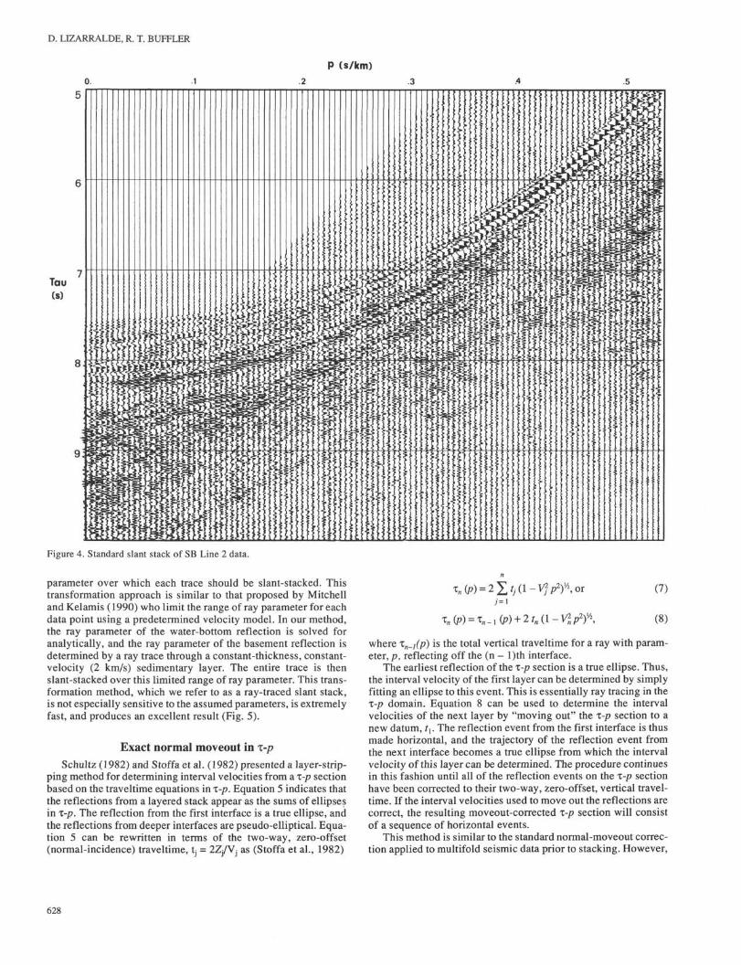
parameter over which each trace should be slant-stacked. Thistransformation approach is similar to that proposed by Mitchelland Kelamis (1990) who limit the range of ray parameter for eachdata point using a predetermined velocity model. In our method,the ray parameter of the water-bottom reflection is solved foranalytically, and the ray parameter of the basement reflection isdetermined by a ray trace through a constant-thickness, constant-velocity (2 km/s) sedimentary layer. The entire trace is thenslant-stacked over this limited range of ray parameter. This trans-formation method, which we refer to as a ray-traced slant stack,is not especially sensitive to the assumed parameters, is extremelyfast, and produces an excellent result (Fig. 5).

Exact normal moveout in x-pSchultz (1982) and Stoffa et al. (1982) presented a layer-strip-

ping method for determining interval velocities from a x-p sectionbased on the traveltime equations in x-p. Equation 5 indicates thatthe reflections from a layered stack appear as the sums of ellipsesin x-p. The reflection from the first interface is a true ellipse, andthe reflections from deeper interfaces are pseudo-elliptical. Equa-tion 5 can be rewritten in terms of the two-way, zero-offset(normal-incidence) traveltime, tj = 2Z/Vj as (Stoffa et al., 1982)

(7)

(8)

where xn_j(p) is the total vertical traveltime for a ray with param-eter, p, reflecting off the (n - l)th interface.

The earliest reflection of the x-p section is a true ellipse. Thus,the interval velocity of the first layer can be determined by simplyfitting an ellipse to this event. This is essentially ray tracing in thex-p domain. Equation 8 can be used to determine the intervalvelocities of the next layer by "moving out" the x-p section to anew datum, tx. The reflection event from the first interface is thusmade horizontal, and the trajectory of the reflection event fromthe next interface becomes a true ellipse from which the intervalvelocity of this layer can be determined. The procedure continuesin this fashion until all of the reflection events on the x-p sectionhave been corrected to their two-way, zero-offset, vertical travel-time. If the interval velocities used to move out the reflections arecorrect, the resulting moveout-corrected x-p section will consistof a sequence of horizontal events.

This method is similar to the standard normal-moveout correc-tion applied to multifold seismic data prior to stacking. However,

628

.2


P (s/km)

.3 4 .5

Tαu(s)

<i i11ii r

Ii j I||

ii

is1

I:

1I . I

11

ii-k

!

h

!;5i

M

i3 Sii

m[vrilisf>i<I

ii•

*

'ill*

•

Biiiir•

ii

rff

f

i

wP;

• ;

<

i: •

iiJ|!1

iiaxf•s

F

1j"

•

•

j !Ii i-J !i |si iiii

M

r

-

Figure 5. Ray-traced slant stack of SB Line 2 data.

the standard normal-moveout correction in X-T is a two-termapproximation to the hyperbolic traveltime equation, which isonly valid for small angles of incidence. The moveout correctionin x-p is exact for all angles. The method is thus referred to asexact normal moveout.

This procedure was carried out using an interactive computerprogram at the University of Texas Institute of Geophysics. Thex-p section is displayed on the computer screen, a normal-inci-dence time is picked for a reflection event, several velocities arechosen and the corresponding ellipses drawn until a good fit tothe event is found. The x-p section is then moved out, and the fitis judged good if the event becomes horizontal. The procedurecontinues until all prominent events have been moved out.

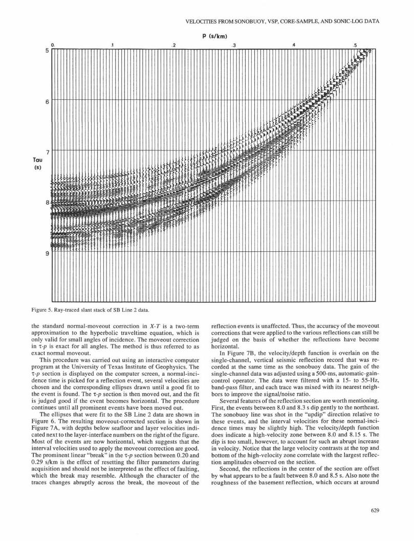
The ellipses that were fit to the SB Line 2 data are shown inFigure 6. The resulting moveout-corrected section is shown inFigure 7A, with depths below seafloor and layer velocities indi-cated next to the layer-interface numbers on the right of the figure.Most of the events are now horizontal, which suggests that theinterval velocities used to apply the moveout correction are good.The prominent linear "break" in the x-p section between 0.20 and0.29 s/km is the effect of resetting the filter parameters duringacquisition and should not be interpreted as the effect of faulting,which the break may resemble. Although the character of thetraces changes abruptly across the break, the moveout of the

reflection events is unaffected. Thus, the accuracy of the moveoutcorrections that were applied to the various reflections can still bejudged on the basis of whether the reflections have becomehorizontal.

In Figure 7B, the velocity/depth function is overlain on thesingle-channel, vertical seismic reflection record that was re-corded at the same time as the Sonobuoy data. The gain of thesingle-channel data was adjusted using a 500-ms, automatic-gain-control operator. The data were filtered with a 15- to 55-Hz,band-pass filter, and each trace was mixed with its nearest neigh-bors to improve the signal/noise ratio.

Several features of the reflection section are worth mentioning.First, the events between 8.0 and 8.3 s dip gently to the northeast.The Sonobuoy line was shot in the "updip" direction relative tothese events, and the interval velocities for these normal-inci-dence times may be slightly high. The velocity/depth functiondoes indicate a high-velocity zone between 8.0 and 8.15 s. Thedip is too small, however, to account for such an abrupt increasein velocity. Notice that the large velocity contrasts at the top andbottom of the high-velocity zone correlate with the largest reflec-tion amplitudes observed on the section.

Second, the reflections in the center of the section are offsetby what appears to be a fault between 8.0 and 8.5 s. Also note theroughness of the basement reflection, which occurs at around

629


P (s/km).2 .3

Tαu

(s)

. E

k

iif

|j

1Å ?

.

!i*

j>I

V

1

a !!1!1!

s!]I11\ii !h3

•

!1|

\L! i;El:- 1

• s1P

ii5\

H

PI

Ii j

i_̂\*

3::i

•

i|i-

s

:i5a

1

13!

::li

3

%

j3-

0 !!1> i

11»

1•Iii

3

38!•11

\\1;

\

•

"i

!

!!

i a

it1>•

\1I1T1

%%

\

\

\• ;

%

tv1\IiAr

i|:::u

SI;

1|sfü7

%

\I?

1!!i

V

I11

•

11jI]iI

As-I!ir55

I\1I

111I11i i

Figure 6. x-/7 section of Figure 5 with fit ellipses drawn in.

8.5 s. The presence of dip and faulting within the sedimentarysection and significant relief of the basement topography mayintroduce some error into the velocity analyses, which assumes ahorizontally stratified media. These features, however, are not toopronounced and probably do not significantly affect the results.

Interval velocities from semblance in X-T

The method of determining interval velocities from stackingvelocities using Dix's (1955) equation is very common in theanalyses of multifold seismic data. The stacking velocity, Vs, isdetermined as that velocity which produces the "best fitting"hyperbola,

reflections from the nth interface (Dix, 1955). The interval veloci-ties can be determined from Dix's equation (1955) as

VftMS, n‰,n~ *RMS, n - H 0, w - 1

Tn „ — 1 ft „ _ 1(10)

'0,n

X2

V2 '(9)

in the sense that the amplitudes of the traces along the hyperbolictrajectory maximize some coherency statistic, typically sem-blance (Taner and Koehler, 1969). Stacking velocities can bechosen for various reflection events from a velocity spectra plot,which is typically a contour plot of semblance values determinedfor a range of velocities at various intercept times. If the stackingvelocities are assumed equal to the RMS velocities, then Equation9 is the two-term approximation to the traveltime equation for

where vn is the interval velocity of layer n.Equation 9 is based on a small-angle approximation which is

only valid for small offset distances. As traces at larger offsets areconsidered, the stacking velocity determined from the best-fithyperbola will diverge from the true RMS velocity. The limitedbandwidth of the data also introduces uncertainties in the deter-mination of stacking velocities and intercept times. Equation 10is sensitive to errors in the values of RMS velocity and intercepttime. Stoffa et al. (1982) presented examples from real and syn-thetic data suggesting that even in the best conditions, errors ininterval velocities determined by this approach can easily be onthe order of 5%-10%.

Figure 8 is a velocity spectra plot of semblance values between0.4 and 1.0. These spectra were calculated from the first 4.5 kmof SB Line 2. The picked zero-offset times and RMS velocitiesused for calculating interval velocities are indicated. The solidline passes through the picked maxima. The spectra indicate anupper interval relatively incoherent events between 7.55 and

630


p (s/km)

7.50. .3

••P•••••••••wp•••••••••• l l•lll•IIIIIIl•lll

m:::zt

8.0<

Tαu(S)

8.5

^

9.0

1 — On, 1.4G6KΠ/S

2 - 4Git, 1 0 466KIVS

3 -– 7Bn, 1.515KMΛ

4 - 119M, JO515KM/S

3 - 192M- 1D521KM/S

6 - 2 3 8 M . U537KM/S

. 7 - 3 0 3 M , 1D934KM/S

. 8 - 3 3 5 M , 1O878KM/S

. 9 - 3 6 9 M , 1D960KM/S

.10 - 4 0 5 M , 1=910KM/S

.11 - 5 0 3 M , 2O323KM/S

.12 - 5 6 1 M . 2C15GKN/S

.13 - 5 9 0 M , 1=924KM/S

.14 - 6 2 2 M , 1C878KM/S

.15 - 66Gπ, 1O960KM/S

.18 - 746n, lα960Kπ/s

.17 - 793π, 1=880KΠ/S

.18 - 942π, 2D200KΠ/S

BNE

7.51SW

8.0<^ρ

TWT

(S)

8.5

9.0JFigure 7. A. Moved-out x-p section with interval velocities and depth below seafloor indicated next to the layer-interface numbers.B. Single-channel reflection section along SB Line 2 (Fig. 1) with the interval-velocity function from (A) superimposed at the left ofthe figure. Northeast is to the left, southwest to the right.

631


1.3 1.4

RMS Velocity (km/s)

1.5 1.6 1.7 1.8

7.5

ZeroOffset

Time(s)

8.0

*̂

<3b7.5C

T6 s. 1.460

7.909.1.

7.982.1.

u 8.06^-

11

\

km/s

468

475

.1.488

47 1.501

8.207 1.

8.296.1.

8.48!

505

510

i. 1.550

8.5

Figure 8. Contour of semblance values from 0.4 to 1.0 (contour interval 0.1). Zero-offset times and RMS velocities used inthe calculation of interval velocities of Figure 9 are indicated. Solid line passes through the picked maxima.

7.85 s. The events between 8.0 and 8.1 s are less coherent thanthe other events in the 7.9-8.35 s interval. This 8.0- to 8.1-sinterval coincides with the high velocity zone (2.32 km/s) deter-mined by the x-p analyses and also coincides with the maximumscatter in the velocities measured from the core samples (dis-cussed below).

The interval velocities determined from the semblance picksare shown in Figure 9 along with the interval velocities deter-mined from the x-p analyses. The two results are generally similar.The velocity of the interval between 750 and 1000 mbsf (metersbelow seafloor) determined from the semblance pick at 8.5 s isconsiderably higher than the velocity determined from the x-panalyses. The semblance values at 8.5 s are somewhat low (0.5),however, which reflects the discontinuous nature of the basementreflection.

The interval velocities determined from the x-p analyses arepreferred because of the better resolution of the method andbecause the method involves no offset-dependent approxima-tions. A similar semblance analyses was performed on the x-ptransformed data, where elliptical trajectory based on RMS ve-locities were scanned. The semblance plot and resulting interval

velocities were virtually identical to those determined from theanalyses of the X-T data.

VELOCITIES FROM VSP, CORE SAMPLES, ANDTHE SONIC LOG

The VSP DataA VSP experiment was conducted in the cased Hole 765D

(Bolmer et al., this volume). The VSP tool occupied 35 stationsspaced 12-30 m apart between 186.0 and 915.0 mbsf. Shots werefired from a 1000 in.3 air gun and a 400 in.3 water gun. During theexperiment, arrivals detected by the VSP geophones were moni-tored in the Underway Geophysics Laboratory, and the tool re-mained at a station until clear signals from at least five shots fromeach gun were recorded. The data from each station were sub-sequently edited, and the good traces stacked to enhance thesignal/noise ratio. The resulting VSP stacked section for the airgun shots is shown in Figure 10.

Interval velocities can be determined from the VSP data bydividing the distance between two stations, dz, by the differenceof the arrival times, dt, of the direct wave recorded at the two

632


Interval velocities from SB Line 2 Travβl (

1.0

Velocity (km/s)1.5 2.o 2.5 3.0

oo

oσ

oO

Q L<D

σo

ooQO

1

1

1

r

;•

I

J

j

Tau-p analysisSemblance analysis

Figure 9. Interval velocities determined from the semblance picks (dashedline) and the x-p analyses (solid line).

stations. The depth of the tool in the hole was determined by thewireline-out depth at the logging winch. The arrival-time differ-ences, or dt's, were determined from similar pulse-phase peaks offirst breaks on adjacent station traces (Bolmer et al., this volume).The velocities determined for the intervals between each VSPstation are plotted as the solid line in Figure 11.

There is a significant amount of variability in the VSP intervalvelocities. The velocity values vary by ±0.1-0.2 km/s about amean of -2.0 km/s. Some of this fluctuation may be a result oferrors in the positioning of the tool in the hole. At a station spacingof 12-30 m, a 1.0-2.0 m error in dz could easily account for thevariation in the interval velocities. Such an error in the determi-nation of the depth of the tool is possible, given the length of thewireline and the difficulties encountered in setting the tool incasing during the experiment (see Bolmer et al., this volume).

The effect of errors in dz will be reduced if velocities arecalculated over larger intervals. However, there will be a loss ofresolution in the velocity profile if the velocities are calculatedover an interval of three VSP stations, say, as opposed to two. Bycomputing a "weighted-average" interval velocity between eachVSP station the effect of errors in dz can be reduced whilemaintaining the resolution of the experimental station spacing.

A weighted-average interval velocity between VSP Stations 2and 3, for example, can be computed as the average of thecomputed interval velocities between Stations 1 and 3 and be-tween Stations 2 and 4. This is, in a sense, a signal-enhancing,

200-

300-

400-

Depth(mbsf)

500

600-

700-

800

900

Figure 10. Stacked, vertical-component VSP section of air-gun arrivals.

low-pass filter, in that noise (the effect of presumably randomerrors in the determination of the depth of the tool) is reduced,while the velocity determined for a particular interval is influ-enced by the velocities of the intervals above and below (as if thevelocity function had been convolved with a triangular operator).The resulting weighted-average interval velocities are plotted inFigure 11 as a heavy, dot-dash line. The fluctuations in thevelocities are reduced and the agreement between the VSP-deter-mined velocities and those determined from the Sonobuoy (light,dashed line) is improved, particularly in the interval between 550and 800 mbsf. The high velocity zone indicated by the VSP resultsbetween 350 and 500 mbsf roughly corresponds with high veloc-ity zone indicated by the Sonobuoy results between 400 and 500mbsf.

Core Sample and Sonic Log Velocities.

Compressional (p-wave) velocities were determined in thelaboratory for core samples by dividing the length of the sampleby the traveltime of a 500-kHz compressional wave through thesample. In general, laboratory-measured velocities differ fromin-situ velocities because of differences in confining pressure,drilling disturbance of the sediments, and changes in pore-fluid

633


1.0

VSP Interval VelocitiesVelocity (km/s)

1.5 2.0 2.5

VSP Inverval VelocitiesWeighted interval averageTau-p analysis

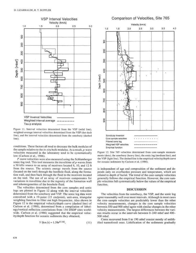
Figure 11. Interval velocities determined from the VSP (solid line),weighted-average interval velocities determined from the VSP (dot-dashline), and the interval velocities determined from the Sonobuoy (dashedline).

conditions. These factors all tend to decrease the bulk modulus ofthe sample relative to the in-situ bulk modulus. As a result,/?-wavevelocities measured in the laboratory tend to be systematicallylow (Carlson et al., 1986).

P-wave velocities were also measured using the Schlumbergersonic-log tool. This tool measures the traveltime of p-waves froma 50 kHz source to an array of receivers located 8, 10, and 12 ftfrom the source. The seismic energy travels from the source(located on the tool) through the borehole fluid, along the forma-tion wall, and then back through the fluid to the receivers locatedon the tool. The use of an array of receivers compensates forvariations in traveltime due to the rugosity of the formation walland inhomogeneities of the borehole fluid.

The velocities determined from the core samples and soniclogs are plotted in Figure 12 along with the interval velocitiesdetermined from the Sonobuoy and VSP. The sonic log data wereconvolved with a 19-point (15 cm/point), unit-area, triangularweighting function to filter out high frequencies. Also shown inFigure 12 is the empirical velocity/depth curve (dashed line) ofCarlson et al. (1986), determined from a compilation of lithol-ogy/vertical-reflection correlations from 154 DSDP sites world-wide. Carlson et al. (1986) suggested that the empirical veloc-ity/depth function for oceanic sediments they obtained,

1.0

Comparison of Velocities, Site 765

Velocity (km/s)

1.5 2.0 2.5 3.0 3.5 4.0

AJ u

%•=—f*—r

\.\

••

Sonobuoy InversionCore sample velocitiesFiltered sonic logWeighted VSP velocitiesEmpirical function

V(km/s)=1.59e(0 33Z>, (11)

Figure 12. Site 765 velocities determined from core-sample measure-ments (dots), the Sonobuoy (heavy line), the sonic log (medium line), andthe VSP (light line). The dashed line is the empirical velocity/depth curvefor oceanic sediments by Carlson et al. (1986).

is independent of age and composition of the sediment and de-pends only on overburden pressure and temperature, which arerelated to depth of burial. The trend of the core-sample velocitiesgenerally follows the empirical function. However, the core sam-ple velocities fall systematically below the values of the empiricalfunction.

DISCUSSIONThe velocities from the Sonobuoy, the VSP, and the sonic log

agree reasonably well over most intervals. Although in most casesthe core-sample velocities are predictably lower than the othervelocity measurements, changes in the core sample velocitiesbetween 550 and 900 mbsf agree with similar changes in the othervelocity measurements. The largest differences between the vari-ous results occur in the intervals between 0-240 mbsf and 400-500 mbsf.

Cores recovered from 0 to 190 mbsf consist mostly of unlith-ified nannofossil ooze. Lithification of the sediments gradually

634


increases from 190 to 379 mbsf, at which depth a fairly markedincrease in lithification occurs. In the interval 0-240 mbsf, thevelocities determined from the Sonobuoy (1.47-1.54 km/s) arenear the velocity of water, reflecting the highly unconsolidatednature of the sediments. However, these velocities are lower thanboth the velocities determined in the laboratory and those pre-dicted by the empirical function. The sonic log data begin atapproximately 190 mbsf, with values of-1.75 km/s, significantlygreater than the other measurements and the empirical function.Thus, the Sonobuoy velocities are probably too low within the0-240 mbsf interval. The empirical function probably gives agood estimate of the velocity to a depth of around 150 mbsf, atwhich point a stronger velocity gradient is necessary to bring thevelocity values nearer those of the sonic log.

The abrupt increase in the Sonobuoy velocity profile at 240mbsf does not coincide with any similarly abrupt change in corelithology. (This depth does roughly coincide, however, with asomewhat abrupt increase in drilling disturbance and decrease incore recovery at 231 mbsf.) Nevertheless, this increase brings theSonobuoy velocities in line with those of the sonic log and VSP.The Sonobuoy and sonic log velocities agree well within the240^00 mbsf interval.

The Sonobuoy velocity profile again abruptly increases at 400mbsf from 1.91 to 2.32 km/s, defining the top of a high-velocitylayer that extends to 500 mbsf. The VSP velocities also increasesignificantly between 325 and 400 mbsf. This increase probablyreflects the increase in lithification observed in the cores at 380mbsf and the presence of a high velocity pebble conglomeratebetween 460 and 475 mbsf. However, the velocities from the VSPin the 400-500 mbsf interval are 0.30 km/s lower than thosedetermined from the Sonobuoy. One explanation for this differ-ence may be a lateral variation in the thickness of the conglomer-ate layer. The scatter of the core-sample velocities illustrates thevariability of the velocities within the conglomerate (some of thevelocities are greater than 4 km/s). Horizontal velocities (whichare measured by the Sonobuoy) may be higher than vertical ve-locities in this interval because of the presence of the high-veloc-ity material within the conglomerate, which may be more exten-sive laterally than directly beneath the drill site. The slight dip ofthe reflections between 8.0 and 8.3 s observed on the single-chan-nel profile may result in slightly higher interval velocity determi-nations from the Sonobuoy.

Given the good agreement of the sonic log, VSP, and core-sam-ple velocities between 500 and 550 mbsf, the Sonobuoy velocitiesin this interval seem somewhat high. Likewise, the VSP velocitiesbelow 800 mbsf seem somewhat low. In general, however, all ofthe velocity measurements agree well below 550 mbsf. Even thesmall changes in the Sonobuoy profile at 600 and 750 mbsf,seemingly below the resolution of the method, appear to beverified by the sonic log and core-sample velocities.

Because the agreement of the Sonobuoy velocities and thoseof the other measurements is good, the Sonobuoy velocities canbe used with confidence to estimate depths to reflections observedon regional multifold seismic profiles. In Figure 13, the Sonobuoyvelocity profile is overlain on a portion of the BMR (AustraliaBureau of Mineral Resources) Rig Seismic Line 56-23C. This linetrends southeast (approximately perpendicular to SB Line 2) andpasses over Site 765 and the closest approach of SB Line 2 to thesite (Fig. 1). The depths to the seismic sequence boundariesinterpreted by Buffler (1989) are indicated at the right of thefigure. These depths can be used to tie the seismic sequences tothe lithologies observed in the cores recovered at Site 765.

CONCLUSIONThe acquisition of Sonobuoy, VSP, sonic log, and core-sample

traveltime data at Site 765 provided a rare opportunity to compare

the velocity information that can be derived from these types ofdata. None of the data are perfect. A change in acquisition param-eters in the middle of the Sonobuoy experiment makes the Sono-buoy data less than ideal. The depths of the VSP stations maycontain significant errors due to the difficulties setting the tool inthe casing and the considerable water depth of the hole. The soniclog data do not cover the entire length of the hole and are sporadicwithin the logged interval. The core samples were affected bydrilling disturbance, and traveltimes were not measured at in-situconditions.

Nevertheless, the resulting velocities from all data types agreewell. Although the velocities determined from the core samplesare generally lower than those determined from the other data, thedifference is systematic and abrupt changes in core-sample veloci-ties generally match similar changes in the other velocity meas-urements. The "scatter" of the interval velocities determined fromthe VSP data associated with uncertainties in the positioning ofthe tool were reduced by computing a weighted-average intervalvelocity between each VSP station. The velocities determined inthis way agree well with the trend of the other velocity determi-nations.

The velocities determined from the Sonobuoy for the interval400-500 mbsf may be somewhat higher than the vertical veloci-ties for similar depths in the vicinity of Site 765. This is probablya result of (1) the presence of high-velocity material within apebble conglomerate at these depths, which may vary laterally,and (2) the presence of a slight dip in the strata at these depths.Below 550 mbsf all of the velocity measurements are in agree-ment.

Of the four types of velocity measurements, the Sonobuoyprofile provides the least direct measure of seismic velocity at aparticular location and depth. However, because it is an indirectmeasure, Sonobuoy data are considerably less difficult and lessexpensive to acquire. The good agreement of these various datatypes is significant in that it provides a verification of the Sono-buoy method, and in particular the x-p approach. These resultssuggest that given good quality data and a reasonably uniformgeologic setting, sonobuoys can be used to determine accurate anddetailed velocity/depth functions.

ACKNOWLEDGMENTSWe thank Warren Wood for his kind assistance in the use of

his "P-Pick" normal moveout program. We acknowledge the inputof Davis Falquist and Richard Carlson, and the assistance of thescientists and marine technicians of Leg 123, who helped acquirethe data for this study.

REFERENCES

Buffler, R. T., 1990. Underway geophysics. In Gradstein, F. M., Ludden,J. N., et al., Proc. ODP, Init. Repts., 123: College Station, TX (OceanDrilling Program), 13-25.

Carlson, R. L., Gangi, A. F., and Snow, K. R., 1986. Empirical reflectiontraveltime versus depth functions for the deep-sea sediment column./ . Geophys. Res., 91:8249-8266.

Diebold, J. B., and Stoffa, P. L., 1981. The traveltime equation, tau-pmapping, and inversion of common midpoint data. Geophysics,46:238-254.

Dix, C. H., 1955. Seismic velocities from surface measurements. Geo-physics, 20:68-86.

McMechan, G., and Ottolini, R., 1980. Direct observation of a p-T curvein a slant stacked wavefield. SSA Bull., 44:1193-1207.

Phinney, R. A., Chowdhury, R. K., and Frazer, L. N., 1981. Transforma-tion and analysis of record sections. / . Geophys. Res., 86:359-377.

Schultz, P. S., 1976. Velocity estimation by wave front synthesis [Ph.D.dissert.]. Stanford Univ., Stanford, CA.

, 1982. A method for direct estimation of interval velocities.Geophysics, 47:1657-1671.

635


Schultz, P. S., and Claerbout, J. F., 1978. Velocity estimation and down-ward continuation by wavefront synthesis. Geophysics, 43:691-714.

Singh, S. C , West, G. F., and Chapman, C. H., 1989. On plane-wavedecomposition: alias removal. Geophysics, 54:1339-1343.

Stoffa, P. L., Buhl, P., Diebold, J. B., and Wenzel, F., 1981. Directmapping of seismic data to the domain of intercept time and rayparameter: a plane wave decomposition. Geophysics, 46:255-267.

Stoffa, P. L., Diebold, J. B., and Buhl, P., 1982. Velocity analysis forwide aperture seismic data. Geophys. Prospect., 30:25-57.

Taner, M. T., and Koehler, F., 1969. Velocity spectra-digital derivationand applications of velocity functions. Geophysics, 34:859-881.

Wood, W., 1989. Seisimic velocities of the Nankai Trough from ESP andSonobuoy Data [M.S. thesis]. Univ. of Texas, Austin.

Date of initial receipt: 31 May 1990Date of acceptance: 11 June 1991Ms 123B-140

1 km

SBL2 Site 765

SE NW

Velocity (km/s)1.41.6 1.8 2.0 2.2 2.4

SeismicSequence

iriiΦui rfiHii• 'iiniiiii ut* i*. ||i

190

2 9 0

4 0 0

510

6 3 0

940

Lith. Graphicunit lith.

IA

IB

IC

II A

MB

IIC

III BIMCIV AIV B

IVC

IVD

V A

VB

VC

VI

VII

-– .400

200

Figure 13. BMR Rig Seismic Line 56-23C with the Sonobuoy velocity profile overlain. Depths to interpreted seismic sequences (Buffler,

1989) indicated at the right of the figure are based on the Sonobuoy results. The graphic lithology column with major lithologic units is

included at the right.

636

Documents

34. COMPARISON OF VELOCITIES DETERMINED FROM SONOBUOY, VSP