Lyapunov based control for non isothermal

continuous stirred tank reactor

H. Hoang ∗F. Couenne ∗C. Jallut ∗Y. Le Gorrec ∗

∗ LAGEP, University of Lyon 1 - UMR CNRS 5007, Bat. 308 G43, Bd du 11 nov. 1918, 69622 Villeurbanne cedex France,

name@lagep.univ-lyon1.fr

Abstract: In this contribution we apply the approach of passivity proposed by Ydstie[M. Ruszkowski, V. Garcia-Osorio, and B.E. Ydstie. AIChE Journal, 2005] for physico-chemicalprocesses. The originality of this work lies in the fact we consider a thermodynamically nonlinearconsistent model for a continuous stirred tank reactor to built the appropriate Lyapunov functionfor stabilization purpose. Indeed the kinetics of reaction modelled by Arhenius law leads to nonlinear model with multiple steady state. We propose to stabilize the reactor around the unstablepoint. In order to apply the Ydstie approach, we assume that the fluid remains homogeneous.This assumption permits to use the concavity property of the entropy function to build theLyapunov function. We propose feedback laws in order to ensure the closed loop properties ofthe Lyapunov function. Finally we propose some simulation results.

Keywords: Lyapunov based control, thermodynamics, Non isothermal CSTR.

1. INTRODUCTION

Control of Continuous Stirred Tank reactor (CSTR) hasbeen widely investigated Luyben [1990], Read [1998], Al-varez [2000], Hua [2000], Guo [2001], Biagiola [2004], Jana[2005]. The underlying motivation relies on the fact thatindustrial chemical reactors may be operated at unstableoperating conditions, which often corresponds to optimalprocess performance. The methodologies used for stabi-lization of such processes are often based on input/output(I/O) feedback linearization Bastin [1997] or nonlinear PIcontrol algorithms Alvarez [1999, 2000]. In this paper wepropose a Lyapunov based approach for the stabilizationof CSTR around an unstable steady state. This approachis based on the recent work of Alonso [1997], Ydstie [1997],Ruszkowski [2005] where a thermodynamical developmentis given in order to obtain a Lyapunov function for trans-port reaction systems. In Ruszkowski [2005] the authorstreat the example of CSTRs in the isothermal case.

2. THERMODYNAMIC ASPECTS

In this section we briefly review the basis of thermody-namics and show how to obtain the so called availabilityfunction. This availability function is a function issuedfrom the second principle of the thermodynamic that isnaturally positive for homogeneous thermodynamical sys-tems. Consequently it is a natural candidate as Lyapunovfunction. We shall show this function issued from thermo-dynamic properties can be used for closed loop dynamicstabilization.

In Ruszkowski [2005] the authors apply fundament of irre-versible thermodynamics in order to produce a Lyapunovfunction for stabilization purposes. Indeed thermodynam-ics is based on the concept of energy as well as Lya-punov functions. Moreover process systems are based for

their modelling on thermodynamics properties. In Ydstie[1997] the authors showed that passivity is related to theavailability function used in thermodynamics for phasestability.

In the case of simple homogeneous thermodynamical sys-tems composed of a mixture of nc species, the fundamentalrelation of thermodynamics expresses the entropy S as afunction of the internal energy U , the volume V and themole number ni by The Gibbs equation:

dS =1

TdU +

P

TdV +

nc∑

i=1

−µi

Tdni (1)

where P , T , µi represent respectively the pressure, thetemperature and the chemical potential of species i. Itis well known that balance equation can be establishedfor U ,V and ni as well as for the entropy S but thislatter is not conservative. let us consider the vector ofextensities ZT = ( U V n1 . . . nc ) and its associatedvector of intensities (homogeneous function of degree 0 of

Z) wT =

(1

T

P

T

−µ1

T. . .

−µc

T

). It then follows that

w =∂S

∂Z. (2)

Remark 1. Gibbs equation (1) differentiation with respectto time permits to link together the different balance by:

dS

dt= wT dZ

dt. (3)

S being a homogeneous function of degree 1 with respectto Z, from Euler’s theorem we can express entropy as:

S = wT Z. (4)

In the case of isolated systems, the entropy balance isreduced to:

Proceedings of the 17th World CongressThe International Federation of Automatic ControlSeoul, Korea, July 6-11, 2008

978-1-1234-7890-2/08/$20.00 © 2008 IFAC 3854 10.3182/20080706-5-KR-1001.3322

dS

dt= σ. (5)

where the entropy production term σ is positive from thesecond law of thermodynamics. The entropy S of an iso-lated system can only increase. In this case the irreversibil-ities will be due to non equilibrium initial conditions overthe considered domain. As a consequence for simple homo-geneous thermodynamical systems, the entropy functionS(z) is necessarily concave (see Callen [1985]) as shown infigure 1.

S(z)

z

z1

Av

z2

Fig. 1. Entropy function with respect to Z and the avail-ability

From these observations, it can be shown (see Ydstie[1997]) that the non negative function Av(Z1) = S(Z2) +wT

2 (Z1−Z2)−S(Z1) is a measure of the distance betweenthe state Z1 and the thermodynamic Z2. The slope of thetangent plane is related to intensive vector.

Remark 2. The availability Av corresponds to the quan-tity involved in the Gibbs’ tangent plane condition: Gibbs(1873) proved that any given mixture at a given temper-ature pressure and overall composition would be globallystable if and only if the tangent to the Gibbs free energysurface (not necessarily concave) would never cut the sur-face. This result is used effectively to solve the multiphaseequilibrium problems. In the case of entropy surface itmeans that Av must be non negative.

In more general case, we get that two states Z and Z2 arein equilibrium if and only if Av(Z) = Z2 = 0.

So as soon as we consider homogeneous mixture, S remainsconcave and A can be considered as a Lyapunov functioncandidate. It remains to set feedback control such that

dAv

dt< 0. (6)

3. DESCRIPTION OF THE CSTR MODEL

In the present paper we consider a CSTR that is connectedto a heat exchanger that is used to control the temperaturewithin the reactor. The dynamics of the stirred tankreactor (STR) can be deduced from mass and energybalances by considering the following assumptions:

• The heat flow exchanged with the jacket is repre-sented by Q (w) and depends on the temperaturesof the jacket Tw and of the reactional mixture in thereactor T : Q = λ(Tw − T ) with λ the heat transfercoefficient (w/K).

• The reaction under consideration A → B takesplace in the reactor in liquid phase. The kinetics ofthe reaction is modelled by the Arrhenius law. Thereaction rate rv is given by k0 exp −E

RTnA

V.

• the reaction mixture is supposed to be ideal.• For simplicity, the two species are supposed to have

the same molar volume vA = vB = v (m3/mol).• At the inlet of the reactor, the pure component A is

injected at temperature Te.• the reaction volume V is supposed to be constant as

well as the pressure P . This implies a constraint onthe total outlet flow. Moreover P is set to Pref .

3.1 CSTR modelling

The mass balance are given by:

dnA

dt= FAe − FA − ξArvV

dnB

dt= −FB + ξBrvV

(7)

where

• nA, nB are the mole number of species A and Brespectively (mol).

• FAe is the inlet molar flow rate of species A (mol/s).• FA, FB are the outlet molar flow rate of species A

and B respectively (mol/s).• ξA, ξB are the stoichiometric coefficient (supposed to

be equal to 1).

let us write the internal energy balance:

dU

dt= Q − P

dV

dt+ FAehAe −

flowing out enthalpy︷ ︸︸ ︷FAhA − FBhB , (8)

where

• U is the internal energy (J).• hAe is the inlet molar enthalpy of species A (J/mol).• hi is the molar enthalpy of species i (i = A,B)) in

the reactor (J/mol).• P is the pressure in the reactor(Pa).

Remark 3. Since we suppose ideality of the mixture, theenthalpy of species in the mixture can be expressedas: hA(T ) = cpA(T − Tref ) + hAref A same expressioncan be written for B. where cpA (J/mol/K) is the heatcapacities of species A, Tref is the reference temperature,hAref is the enthalpy of reference of species. Let us notefurthermore that, as the species are involved in a chemicalreaction, the reference molar enthalpies have to be chosenwith regard to the enthalpy of formation of species.

Finally the volume balance is given by:dV

dt= 0 (9)

Moreover the volume is also given by: V =∑

i=A,B nivi.Deriving this expression and equating to zero, the totaloutput flow rate F is deduced. Since FA = xA F andFB = xB F where xA and xB represent the mole fractionof species A and B respectively, we get:

F =vAFAe + (ξBvB − ξAvA)rvV

xAvA + xBvB

(10)

Remark 4. let us note that xA = nAv

V

17th IFAC World Congress (IFAC'08)Seoul, Korea, July 6-11, 2008

3855

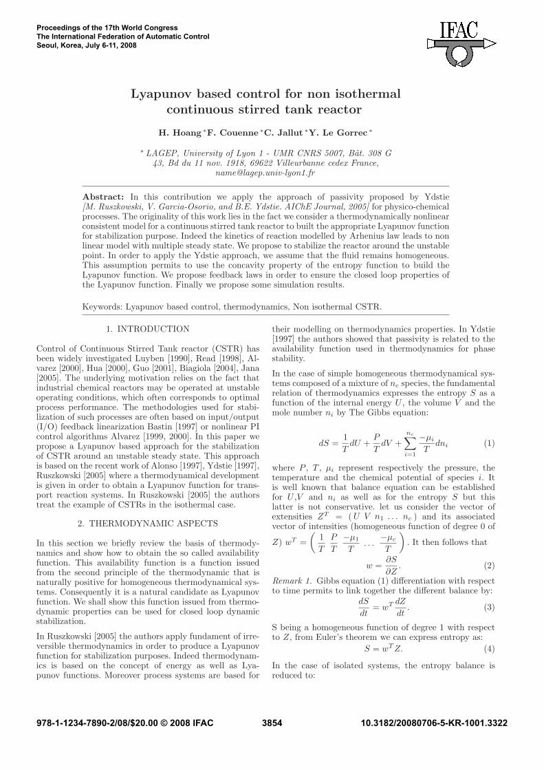
3.2 Analysis of the steady states

A most interesting feature of this reactor that createscontrol difficulty is its multiple steady states. Figure 1illustrates this feature clearly. There are three steadystate operating points: P1, P2 and P3. The steady stateoperating points P1 and P3 are stable, whereas the steadystate operating point P2 is not stable. The reactor isoperated at unstable steady state operating point P2 whichis at medium conversion. Manipulated variables are chosenas:

FAe = 0.0183mole

s, Te = 310 K and Tw = 300 K (11)

The steady state points are computed using equations 7and 8 considering dna

dt= dnb

dt= U

dt= 0 and the relation

between U and T . The steady states operating points are:

[nA nB T ] = [1.6449 0.3551 320.6704] (P1)

[nA nB T ] = [1.3583 0.6417 330.1997] (P2)

[nA nB T ] = [0.1416 1.8584 377.8795] (P3)

as shown in figure 2, where F corresponds to the rightmember of the differential equation written with respectto temperature T :F = (hA − hB) rvV + FAeCpA (Te − T ) + λ (Tw − T ).

310 320 330 340 350 360 370 380−4

−2

0

2

4

6

8

10Equilibrium points/Steady states

T

F(T

)

Fig. 2. Steady states reactor temperature vs. F(T)

3.3 Controller synthesis

The control objective of this system is to maintain thereactor temperature T as well as mole number nB at theirdesired value by manipulating the coolant temperature Tw,the inlet molar flow rate of species A FAe as well as itstemperature Te. Te appears in the inlet enthalpy of speciesA hAe.

The availability function has to be written with w =(1

T, P

T,−µA

T,−µB

T

)et Z = (U, V, nA, nB). Nevertheless

since the reactional scheme is very simple with constantvolume and same molar volume for species, we have theconstraint between nA and nB :

−

dnA

dt=

dnB

dt(12)

and with (9), we can rewrite A with w =(

1

T,−µA

T+ µB

T

)

et Z = (U, nA).

Let us rewrite the availability function of this process withrespect to P2: A(Z) = S2 + wT

2 (Z − Z2) − S(Z). Fromequation (4), we obtain:

dAv

dt= −(w − w2)

T dZ

dt(13)

Considering the deviation variable w = w − w2, (13) canbe expressed by:

dAv

dt= −wT dZ

dt(14)

dAv

dt= −wT

(Q + FAehAe − FAhA − FBhB

FAe − FA − rvV

)(15)

With simplifying assumptions 1 molar volume and stoi-chiometric coefficient the total molar flow rate becomes:

F = vFAe (16)

and we get

dAv

dt= −wT

(Q(Tw) + F(Te)FAe

GFAe − rvV

)(17)

with F = hAe(Te) − v(xAhA(T ) + (1 − xA)hB(T )),G = 1 − vxA

The objective is to set feedback control on the manipulatedvariables Tw, TE and FAe such that dAv

dt< 0. It is done

expressing dAdt

as a semi definite negative quadratic formrespect to the variables w. Let us choose:

Q = −K1

(1

T−

1

T2

). (18)

From this equation, the manipulated temperature feed-back law Tw is deduced as:

Tw =K1

λ

(1

T−

1

T2

)+ T (19)

Te is chosen such that F = F(Te, T, nA, nB) = 0. FinallyFAe is chosen such that:

FAe = G−1

(rvV + K2

˜(−µA

T+

µB

T

))(20)

Where

˜(−µA

T+

µB

T

)=

(−µA

T+

µB

T

)−

(−µA2

T2

+µB2

T2

)

We then obtain:

dAv

dt= −wT Kw (21)

1 Even if they simplify the notation, these assumptions are notnecessary for the design of the control law.

17th IFAC World Congress (IFAC'08)Seoul, Korea, July 6-11, 2008

3856

with K =

(K1 0

0 K2

).

Since the Ki’s are chosen strictly positive clearly dAv

dt< 0

so Av tends exponentially to zero.

3.4 Simulation

The purpose of this section is to illustrate the stabilizationprocedure on a simple but realistic example. Parametersused for simulation are given in table 1 and simulationsare carried out using Matlab Simulink software.

Numerical valueCpA 75.24CpB 60.E 1046.43hAref 0hBref -4575k0 0.12 1010

P 105

Pref 105

R 8.314(J/K/mol)Tref 300v 0.0005V 0.001λ 0.05808sAref 210.4sBref 180.2ξA 1ξB 1

Table 1. Steady-state design parameters

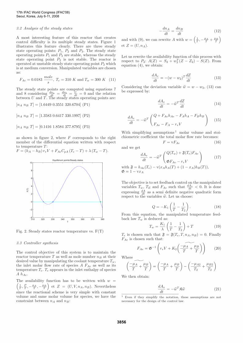
First of all let us consider open loop simulation with input(11) and initial state P2. As operating point P2 is the mostinteresting from industrial point of view we do simulationsaround this point. Let us note that P2 corresponds toa good advancement of the reaction and to a moderatetemperature which is usually necessary to preserved goodquality of polymers for example. This steady state istypically unstable. From any point of the operating domainthe system can go to the stable steady state P1 wherethe reaction is shutting down (law temperature) or tothe stable steady state P3 if the reaction go faster (hightemperature). The operating point P2 is very sensitiveto small variations or errors on the initialization. Indeeddespite high accuracy in the steady state computation (sayprecision around 10−5) the system accumulate numericalerrors and tends after a certain time to the nearest steadystate point P1 (see Figure 3).

0 1000 2000 3000 4000 5000 6000 7000320

322

324

326

328

330

332

0 1000 2000 3000 4000 5000 6000 70001.35

1.4

1.45

1.5

1.55

1.6

1.65

1.7

Fig. 3. Open loop simulations around the unstable steadystate. Reactor temperature (lhs) and number of molesof species A (rhs) vs. time)

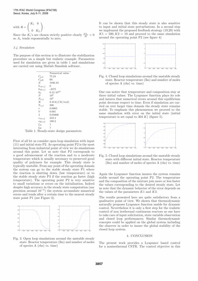
It can be shown that this steady state is also sensitiveto input and initial state perturbations. In a second stepwe implement the proposed feedback strategy (19,20) withK1 = 500,K2 = 10 and proceed to the same simulationaround the operating point P2 (see figure 4)

0 1000 2000 3000 4000 5000 6000 7000329

329.5

330

330.5

331

331.5

0 1000 2000 3000 4000 5000 6000 70000

0.5

1

1.5

2

2.5

Fig. 4. Closed loop simulations around the unstable steadystate. Reactor temperature (lhs) and number of molesof species A (rhs) vs. time)

One can notice that temperature and composition stay atthere initial values. The Lyapunov function plays its roleand insures that numerical errors around this equilibriumpoint decrease respect to time. Even if simulation are car-ried on over larger time domain the steady state remainsstable. To emphasis this phenomenon we proceed to thesame simulation with error on the initial state (initialtemperature is set equal to 304 K) (figure 5).

0 1000 2000 3000 4000 5000 6000 7000295

300

305

310

315

320

325

330

0 1000 2000 3000 4000 5000 6000 70001.15

1.2

1.25

1.3

1.35

1.4

Fig. 5. Closed loop simulations around the unstable steadystate with different initial state. Reactor temperature(lhs) and number of moles of species A (rhs) vs. time)

Again the Lyapunov function insures the system remainsstable around the operating point P2. The temperatureand the composition of the mixture join more or less fasterthe values corresponding to the desired steady state. Letus note that the dynamic behavior of the error depends onthe values of the parameters K1 and K2.

The results presented here are quite satisfactory from aqualitative point of view. We shown that thermodynamicnaturally proposes Lyapunov function usable for dynamiccontrol. Nevertheless it is only a first step for the realisticcontrol of non isothermal continuous reactors as one haveto take care of input solicitation, state variable observationand closed loop performances. Similar thermodynamicconcepts could be applied on the global system includingthe observer in order to insure the global stability of theclosed loop system.

4. CONCLUSION

The present work provides a Lyapunov based controlfor a nonisothermal CSTR. The control objective in this

17th IFAC World Congress (IFAC'08)Seoul, Korea, July 6-11, 2008

3857

simulation-based work is to maintain the CSTR at steadystate operating point. The main difficulty arises when theoperating point is unstable. This study is a first attempt tobuild a Lyapunov function for thermodynamical coherentCSTR from Ydstie’s work (Ydstie [1997], Alonso [1997],Ruszkowski [2005]). Clearly the control feedback must beimproved: two manipulated variables must be used insteadof three. Moreover this controller must be coupled with anobserver since all the state variables are used.

REFERENCES

B.E. Ydstie, and A.A. Alonso. Process systems andpassivity via the Clausius-Planck inequality. SystemsControl Letters, 30(5):253-264, 1997.

A.A. Alonso, and B.E. Ydstie. Process systems, passivityand the second law of thermodynamics. Computers andChemical Engineering, 20(2):1119-1124, 1996.

M. Ruszkowski, V. Garcia-Osorio, and B.E. Ydstie. Pas-sivity based control of transport reaction systems.AIChE Journal, 51:31473166, 2005.

B. Guo, A. Jiang, X. Hua, X., and A. Jutan. Nonlinearadaptive control for multivariable chemical processes.Chemical Engineering Science, 56:67816791, 2001.

M.A. Henson. Nonlinear Model Predictive Control: Cur-rent Status and Future Directions. Computers andChemical Engineering, 23:187-202, 1998.

X. Hua, and A. Jutan. Nonlinear Inferential CascadeControl of Exothermic Fixed-bed Reactors. AICHEJournal, 46:980-996, 2000.

A.K. Jana, A.N. Samanta, and S. Ganguly. Globallylinearized control on diabatic continuous stirred tankreactor: a case study. ISA Transactions, 44:423-444,2005.

K.J. Kim, and K.Y. Choi. On-line estimation and controlof a continuous stirred tank polymerization reactor.Journal Process Control, 1:96-110, 1991.

C. Kravaris, and C.B. Chung. Nonlinear state feedbacksynthesis by global input/output linearization. AICHEJournal, 33:592-603, 1987.

P.L. Lee, and G.R. Sullivan. Generic Model Control(GMC). Computers and Chemical Engineering, 12:573-580, 1988.

W.L. Luyben. Process Modeling, Simulation, and Controlfor Chemical Engineers. McGraw-Hill, Singapore, 1990.

L. Magni, G. De Nicolao, L. Magnani,and R. Scattolini. Astabilizing model-based predictive control algorithm fornonlinear systems. Automatica, 37:1351-1362, 2001.

N.K. Read, and W.H. Ray. Application of nonlineardynamic analysis to the identification and control ofnonlinear systemsIII. n-Dimensional systems. Journalof Process Control, 8(1):35-46, 1998.

J. Alvarez-Ramirez, and A. Morales. PI control of contin-uously stirred tank reactors: stability and performance.Chemical Engineering Science, 55(22):5497-5507, 2000.

C.T. Chen, and C.S. Dai. Robust controller design for aclass of nonlinear uncertain chemical processes. Journalof Process Control, 11(5):469-482, 2001.

S.I. Biagiola, and J.L. Figueroa. A high gain nonlinearobserver: application to the control of an unstable non-linear process. Computers and Chemical Engineering,28(9):1881-1898, 2004.

F. Viel, and F. Jadot, and G. Bastin. Global stabilizationof exothermic chemical reactors under input constraints

Automatica, 33(8):1437-1448, 1997.J. Alvarez-Ramirez, and R. Femat. Robust PI stabilization

of a class of chemical reactors. Systems & ControlLetters, 38(4-5):219-225, 1999.

H.B. Callen. Thermodynamics and an introduction tothermostatics. JohnWiley & Sons Inc, 2nd ed. NewYork, 1985.

17th IFAC World Congress (IFAC'08)Seoul, Korea, July 6-11, 2008

3858