Embed Size (px)
Citation preview

Ec 655, 3.3. Renewable resources: the fishery 1
3.3 Renewable Resources: The Economics of the Fishery A. Introduction Some historical data:
Canadian Commercial Catch
0500,000
1,000,0001,500,0002,000,0002,500,000
1975 1980 1985 1990 1995 2000 2005
year
$'00
0 or
tonn
es o
f fis
h
Quantity (tonnes) Value, $ thousands
Figure 1 Canadian fish landings and value
Data Source: Department of Fisheries and Oceans, Government of Canada. http://www.dfo-mpo.gc.ca/communic/statistics/main_e.htm Note that the value estimate is in current dollars. To get a true picture we should deflate the data with a price index like the CPI.

Ec 655, 3.3. Renewable resources: the fishery 2
Figure 2 Total World Fishery Production by Region; Source: Food and Agricultural Organization of the United Nations (FAO), http://www.fao.org/fi/fifacts/plots/default.asp
Figure 3 Aquaculture and Capture Fishery Production in 1996, Source: Food and Agricultural Organization of the United Nations (FAO), http://www.fao.org/fi/fifacts/plots/default.asp

Ec 655, 3.3. Renewable resources: the fishery 3
- major source of protein for many communities - An important source of employment for some communities and regions - Technological change has greatly increased catches and reduced costs
- Nylon filament reduced cost of nets
- Refrigeration allows catches to be stored onboard
- Satellites and computer technology to pinpoint fish migrating
- Overexploitation and environmental change such as pollution have caused
populations of many important species of fish to decline markedly in the last several decades – e.g. cod, halibut, haddock.
- We may still see increased catches due to lower valued fish being caught.
- Increased conflicts among user groups
- Competition among fishing nations for stocks outside each country’s 200 mile
limit
- Conflict between commercial and recreational fisheries. B. A Model of the Fishery Simplifying assumptions: a fishery in a particular region with one type of fish harvested by homogeneous vessels all originating from a particular port. Demersal fish – groundfish – lobster, oysters, flounder, cod Pelagic fish – migrate over a wide area of the ocean A renewable resource Reproductive potential of fish depends on size of fish population and characteristics of habitat – assume habitat characteristics held constant for the moment
Population or stock is measured in biomass (weight) units, not by number of individuals – growth can occur through the production of new individuals or growth of existing individuals.

Ec 655, 3.3. Renewable resources: the fishery 4
B.1 Fishery Populations: Biological Mechanics
- assume growth rate of the stock depends on its size - small population – births outnumber deaths because of large food supply - as biomass rises deaths rise as food per creature diminishes - growth rate declines – eventually deaths may equal births and the growth rate
falls to zero. - There may be a minimum size of stock necessary to maintain a viable
population. - X(t) is the stock of fish
/ ( )dX dt F x= (1)
F(x) is the instantaneous rate of growth of the biomass of the fish population

Ec 655, 3.3. Renewable resources: the fishery 5
( ) 0 if 0 1( ) 0 if K1 2( ) 0 if K2
F X X KF X X KF X X
≤ ≤ ≤> ≤ ≤≥ ≤
Purely compensatory growth function: Depensatory growth function: A growth curve exhibiting critical dispensation: Logistic Growth Function:
( ) (1 / )F x rX X k= − (2)
- r is the intrinsic instantaneous growth rate of the biomass - k is the carrying capacity of the habitat - Sketch the logistic growth curve in the figure below.
F(X)
X K1 K2
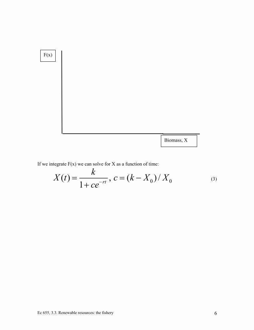
Ec 655, 3.3. Renewable resources: the fishery 6
If we integrate F(x) we can solve for X as a function of time:
0 0( ) , ( ) /1 rt
kX t c k X Xce−= = −
+ (3)
F(x)
Biomass, X
Ec 655, 3.3. Renewable resources: the fishery 7
If there is no harvesting we can find the value of X which represents a steady state i.e. dX/dt = F(X) = 0 What is this steady state level for the fish stock? Discrete time analogue:
1 (1 )t t tt
KX X rXX+ − = − (4)
Can produce complex behaviour depending on value of r – see Conrad and Clark, p. 64 for details. B2. Bionomic Equilibrium in a Simple Model - an equilibrium that combines biological mechanics with economic activity - assume harvesting is costless - How do different harvest rates affect the fish population?
time
X

Ec 655, 3.3. Renewable resources: the fishery 8
Case I: Mining the fishery – draw a harvest rate (h1) that is everywhere above F(x) If the X0=k, what happens to the fish stock once harvesting starts? Case II: Draw a harvest rate (h2) that allows us to obtain the maximum sustained yield. If the X0=k, what happens to the fish stock once harvesting starts? Case III: Sketch a harvest rate line at F(X1) – label it h3 What if X0=k?
F(x)
Biomass, X kX1
F(X1)
X2

Ec 655, 3.3. Renewable resources: the fishery 9
What if X0 is slightly greater than X1? What if X0 is slightly less than X1? For h3, which stock level represents a stable equilibrium and which represents an unstable equilibrium? The effects of harvesting on the fish population can be summarized by:
/ ( ) ( )dX dt F X H t= − (5)
C. Harvest level as a function of effort
- Assume perfectly competitive industry and each firm takes all prices, including factor prices as given and constant over time - implies demand for fish and supply of factors are perfectly elastic Define harvesting function h(t):
( ) [ ( ), ( )]( ) = fishing effort( ) = stock
H t G E t X tE tX t
=
(6)
Effort refers to an index of capital, labour, energy and material inputs. Eg. Number of lobster traps used.

Ec 655, 3.3. Renewable resources: the fishery 10
Consider how h varies with E, for a given (steady state) fish stock.
Figure 4 Harvest versus fishing effort Now consider how harvest is affected when the stock is varied given a fixed level of effort. Harvest will be an increasing function of the fish stock – assume it is linear for simplicity. A commonly used harvest function is:
( ) ( ) ( )h t qE t X t= (7) This function is based on two assumptions: a) Catch per unit of effort is directly proportional to the density of fish in the sea b) the density of fish is directly proportional to the abundance, X(t)
Harvest, h
Effort, E

Ec 655, 3.3. Renewable resources: the fishery 11
With effort level of E1, what is the steady state fish stock? What if the effort level is increased? It is inefficient for the fishing industry to exert a total effort that results in a stock to the left of MSY. Why is this so? We want to plot total revenue and total cost of fishing versus fishing effort. Suppose:
, c is a constant, let P=1
TC cETR Ph
TR h
==
⇒ =
F(x)
Biomass, X k
h=G(E1,X)
Xmsy
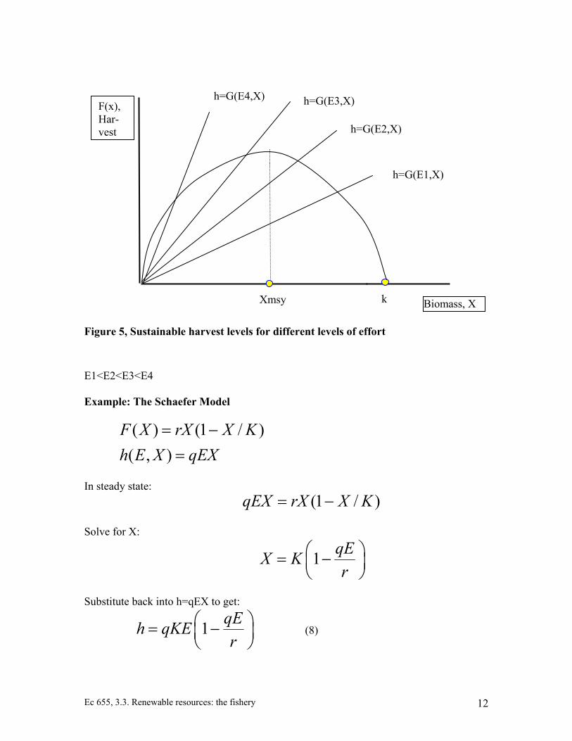
Ec 655, 3.3. Renewable resources: the fishery 12
Figure 5, Sustainable harvest levels for different levels of effort E1<E2<E3<E4 Example: The Schaefer Model
( ) (1 / )( , )
F X rX X Kh E X qEX
= −=
In steady state:
(1 / )qEX rX X K= − Solve for X:
1 qEX Kr
= −
Substitute back into h=qEX to get:
1 qEh qKEr
= −
(8)
F(x), Har-vest
Biomass, X k
h=G(E1,X)
Xmsy
h=G(E2,X)
h=G(E3,X) h=G(E4,X)

Ec 655, 3.3. Renewable resources: the fishery 13
Plot the sustainable yield associated with each of harvest levels. Note that for sufficiently high effort the yield is zero. (E≥r/q)
Figure 6 Sustainable Harvest as a function of effort. Since the price of fish is 1, the harvest shown in the above graph is identical to total revenue. Now add a line showing TC=cE. D. Objectives of Management - a common objective is to maintain the stock that allows the MSY - MSY is where ( ) 0F X′ = - For the Schaefer model this MSY is as follows:
/ 2/ 4
MSY
MSY
X Kh rK
=
=
Harvest and revenue
Effort, E

Ec 655, 3.3. Renewable resources: the fishery 14
- MSY polices have been criticized because
• An overestimate of MSY can lead to depletion or extinction • MSY is not sustainable in the long run, because of natural fluctuations in stock • May not make sense when 2 or more independent species are being harvested. • MSY ignores social and economic considerations • MSY ignores nonmarket “preservation” values General management problem to maximize net social benefits from harvesting the resource.
0maximize ( ( ), ( ))
T tU H t X t e dtδ−∫ (9)
subject to
0
( ( )) ( ( ), ( ))(0)
X F X t h X t E tX X= −
= (10)
Current valued Hamiltonian
( , ) [ ( ) ]H U X Y F x hµ= + − (11) Necessary conditions of the maximum principle:
(a) h( ) maximizes ( , ; ) for all t.(b) X X X
t H X HH U F
µµ δµ δµ µ= − = − −
(12)
D.1 Constant price - no preservation value
( , ) ( , )U X E ph X E cE= − (13) - Maximization problem:

Ec 655, 3.3. Renewable resources: the fishery 15
0maximize { ( ( ), ( )) ( )}
T tph X t E t cE t e dtδ−−∫ (14)
subject to
0
( ( )) ( ( ), ( ))(0)
X F X t h X t E tX X= −
=(15)
We choose h to maximize H :
( ) ( )cH p h F xqX
µ µ= − − +
Suppose ( )( )
ct pqX t
µ = − (17)
Differentiate (17) to get: Use adjoint equation and sub in for µ(t): This gives an expression that defines the solution to our maximization problem. Any X which satisfies this expression is called a singular solution to the original control problem. The X* that satisfies this equation represents the optimal equilibrium stock level. If we are not at X* then the appropriate dynamic adjustment is:
max
0 when ( ) * ( )
h when X(t)>X*X t X
h t<
=
(18)
Procedure for finding the MRAP solution summarized on page 76 of Conrad and Clark.

Ec 655, 3.3. Renewable resources: the fishery 16
D.2 Downward sloping demand curve
( , ) ( )
( )
U X h B h cEcYB hqX
= −
= − (19)
where ( )
0( ) ( )
h tB h D s ds= ∫ .
( ) [ ( ) ]chH B h F x hqX
µ= − + − (20)

Ec 655, 3.3. Renewable resources: the fishery 17
E. Open access equilibrium
Figure 7 What level of effort would be expected in the open access fishery?
h qEX= (21)
( )X F X h= − (22)
( , ) ( )U X E ph cE pqX c E= − = − (23)
(1 )qEh Kr
= − (24)
We can also draw MR, AR, and MC curves.
Harvest and revenue
Effort, E E1 E2 E3 E4
TC=cE
TR=h
Ec 655, 3.3. Renewable resources: the fishery 18
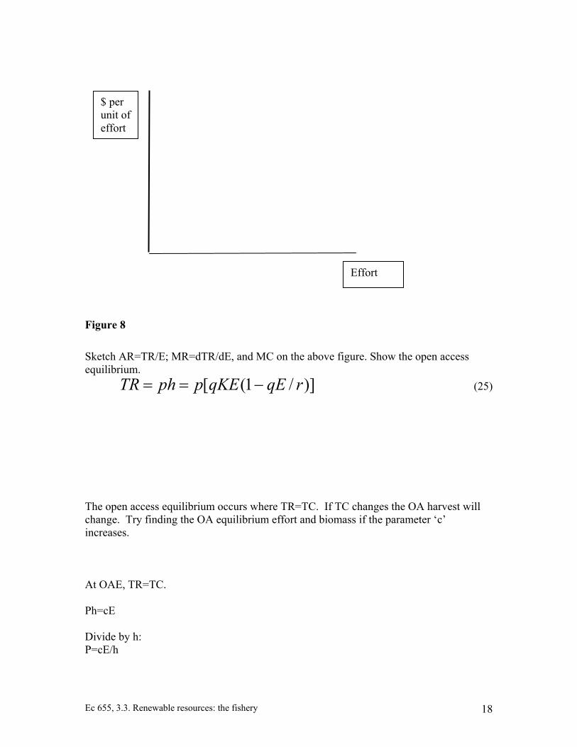
Figure 8 Sketch AR=TR/E; MR=dTR/dE, and MC on the above figure. Show the open access equilibrium.
[ (1 / )]TR ph p qKE qE r= = − (25) The open access equilibrium occurs where TR=TC. If TC changes the OA harvest will change. Try finding the OA equilibrium effort and biomass if the parameter ‘c’ increases. At OAE, TR=TC. Ph=cE Divide by h: P=cE/h
$ per unit of effort
Effort

Ec 655, 3.3. Renewable resources: the fishery 19
At the OAE, price equals the average cost of harvest. At the OAE, MR<MC → Economically inefficient Also if biomass is to the left of that implied by MSY, it is inefficient in a bioeconomic sense. The same harvest could be maintained at a higher biomass of fish.
D. Socially optimal harvest under private property rights Under open access each individual firm (fisher) treats the stock, X, as exogenous. When a firm exerts additional effort it leads to a lower equilibrium stock and a slightly higher harvest cost for every boat. This is a stock effect, an external cost imposed on other firms that is ignored by each individual firm. Results in economic inefficiency. Another possible externality – instead of fixed costs per unit of effort, marginal harvesting costs might depend on the total effort in the fishing industry and on the stock. Congestion costs – another reason the OAE will be inefficient. Three diagrams on the next page show relevant cost and revenue curves for a sole owner. Identify the private property (PPE) equilibrium and compare with the OAE.

Ec 655, 3.3. Renewable resources: the fishery 20
Figure 9 The sole owner will maximize profits by choosing the level of effort where:
Effort, E
Effort, E
Biomass, X
Total revenue and cost, $
$ per unit effort
F(X) and h
TC=cE
ARMR
MC=c

Ec 655, 3.3. Renewable resources: the fishery 21
Compare the amount of effort used in an OAE versus a sole owner. Compare the harvest level under an OAE versus a sole owner.