3238 IEEE TRANSACTIONS ON INFORMATION THEORY… · 3238 IEEE TRANSACTIONS ON INFORMATION THEORY, VOL. 60, NO. 6, JUNE 2014 The Lossy Common Information of Correlated Sources Kumar

3238 IEEE TRANSACTIONS ON INFORMATION THEORY, VOL. 60, NO. 6, JUNE 2014

The Lossy Common Information ofCorrelated Sources

Kumar B. Viswanatha, Student Member, IEEE, Emrah Akyol, Member, IEEE, and Kenneth Rose, Fellow, IEEE

Abstract— The two most prevalent notions of common informa-tion (CI) are due to Wyner and Gács–Körner and both the notionscan be stated as two different characteristic points in the losslessGray–Wyner region. Although the information theoretic charac-terizations for these two CI quantities can be easily evaluated forrandom variables with infinite entropy (e.g., continuous randomvariables), their operational significance is applicable only to thelossless framework. The primary objective of this paper is togeneralize these two CI notions to the lossy Gray–Wyner network,which hence extends the theoretical foundation to general sourcesand distortion measures. We begin by deriving a single lettercharacterization for the lossy generalization of Wyner’s CI,defined as the minimum rate on the shared branch of the Gray–Wyner network, maintaining minimum sum transmit rate whenthe two decoders reconstruct the sources subject to individualdistortion constraints. To demonstrate its use, we compute theCI of bivariate Gaussian random variables for the entire regimeof distortions. We then similarly generalize Gács and Körner’sdefinition to the lossy framework. The latter half of this paperfocuses on studying the tradeoff between the total transmit rateand receive rate in the Gray–Wyner network. We show thatthis tradeoff yields a contour of points on the surface of theGray–Wyner region, which passes through both the Wyner andGács–Körner operating points, and thereby provides a unifiedframework to understand the different notions of CI. We furthershow that this tradeoff generalizes the two notions of CI to theexcess sum transmit rate and receive rate regimes, respectively.

Index Terms— Common information, Gray-Wyner network,multiterminal source coding.

I. INTRODUCTION

THE quest for a meaningful and useful notion of com-mon information (CI) of two discrete random vari-

ables (denoted by X and Y ) has been actively pursued by

Manuscript received January 16, 2013; revised January 13, 2014; acceptedMarch 13, 2014. Date of publication April 4, 2014; date of current versionMay 15, 2014. This work was supported by the National Science Foundationunder Grant CCF-1016861, Grant CCF-1118075, and Grant CCF-1320599.The material in this paper was presented in part at the IEEE InformationTheory Workshop (ITW) at Paraty, Brazil, Oct 2011 and the IEEE Interna-tional Symposium on Information Theory (ISIT) at Boston, MA, USA, Jul2012.

K. Viswanatha was with the Electrical and Computer Engineering Depart-ment, University of California at Santa Barbara, Santa Barbara, CA 93106USA. He is now with the Qualcomm Research Center, San Diego, CA 92121USA (e-mail: [email protected]).

E. Akyol is with the Electrical and Computer Engineering Department,University of California at Santa Barbara, Santa Barbara, CA 93106 USA andwith the Electrical Engineering Department, University of Southern California,Los Angeles, CA 90089 USA (email: [email protected]).

K. Rose is with the Electrical and Computer Engineering Department,University of California at Santa Barbara, Santa Barbara, CA 93106 USA(e-mail: [email protected]).

Communicated by A. Wagner, Associate Editor for Shannon Theory.Color versions of one or more of the figures in this paper are available

online at http://ieeexplore.ieee.org.Digital Object Identifier 10.1109/TIT.2014.2315805

Fig. 1. The Gray-Wyner network.

researchers in information theory for over three decades.A seminal approach to quantify CI is due to Gács andKörner [1] (denoted here by CGK(X, Y )), who defined itas the maximum amount of information relevant to bothrandom variables, one can extract from the knowledge ofeither one of them. Their result was of considerable the-oretical interest, but also fundamentally negative in nature.They showed that CGK(X, Y ) is usually much smaller thanthe mutual information and is non-zero only when the jointdistribution satisfies certain unique properties. Wyner proposedan alternative notion of CI [2] (denoted here by CW (X, Y ))inspired by earlier work in multi-terminal source coding [3].Wyner’s CI is defined as:

CW (X, Y ) = inf I(X, Y ; U) (1)

where the infimum is over all random variables, U , suchthat X ↔ U ↔ Y form a Markov chain in that order.He showed that CW (X, Y ) is equal to the minimum rateon the shared branch of the lossless Gray-Wyner network(described in section II-A and Fig. 1), when the sum rate isconstrained to be the joint entropy. In other words, it is theminimum amount of shared information that must be sent toboth decoders, while restricting the overall transmission rateto the minimum, H(X, Y ).

We note that although CGK(X, Y ) and CW (X, Y ) weredefined from theoretical standpoints, they play important rolesin understanding the performance limits in several practicalnetworking and database applications, see eg., [4]. We furthernote in passing that several other definitions of CI, withapplications in different fields, have appeared in the literature[5] and [6], but are less relevant to us here.

Although the quantity in (1) can be evaluated for randomvariables with infinite entropy (eg. continuous random vari-ables), for such random variables it lacks the underlying the-oretical interpretation, namely, as a distinctive operating point

0018-9448 © 2014 IEEE. Personal use is permitted, but republication/redistribution requires IEEE permission.See http://www.ieee.org/publications_standards/publications/rights/index.html for more information.

VISWANATHA et al.: LOSSY CI OF CORRELATED SOURCES 3239

in the Gray-Wyner region, and thereby mismatches Wyner’soriginal reasoning. This largely compromises its practicalsignificance and calls for a useful generalization which can beeasily extended to infinite entropy distributions. Our primarystep is to characterize a lossy coding extension of Wyner’sCI (denoted by CW (X, Y ; D1, D2)), defined as the minimumrate on the shared branch of the Gray-Wyner network atminimum sum rate when the sources are decoded at respectivedistortions of D1 and D2. Note that the minimum sum rate atdistortions D1 and D2 is given by Shannon’s rate distortionfunction, hereafter denoted by RX,Y (D1, D2). In this paper,our main objective is to derive an information theoretic char-acterization for CW (X, Y ; D1, D2) for general sources anddistortion measures. Using this characterization, we derivethe lossy CI of two correlated Gaussian random variablesfor the entire regime of distortions. This example highlightsseveral important characteristics of the lossy CI and challengesthat underlie optimal encoding in the Gray-Wyner network.We note that although there is no prior work on characterizingCW (X, Y ; D1, D2), in a recent work [7], Xu et al. providedan asymptotic definition for CW (X, Y ; D1, D2)1 and showedthat there exists a region of small enough distortions whereCW (X, Y ; D1, D2) coincides with Wyner’s single letter char-acterization in (1). We further note that there have been otherphysical interpretations of both notions of CI, irrespective ofthe Gray-Wyner network, including already in [1] and [2],whose connections with the lossy generalizations we considerherein are less direct and beyond the scope of this paper.

The last section of the paper focuses on the tradeoffbetween the total transmit rate and receive rate in theGray-Wyner network, which directly relates the two notionsof CI. Although it is well known that the two definitions of CIcan be characterized as two extreme points in the Gray-Wynerregion, no contour with operational significance is knownwhich connects them. We show that the tradeoff betweentransmit and receive rates leads to a contour of points on theboundary of the Gray-Wyner region, which passes through theoperating points of both Wyner and Gács-Körner. Hence, thistradeoff plays an important role in gaining theoretical insightinto more general notions of shared information. Beyond theo-retical insight, this tradeoff also plays a role in understandingfundamental limits in many practical applications includingstorage of correlated sources and minimum cost routing fornetworks (see eg., [4]). Motivated by these applications, weconsider the problem of deriving a single letter character-ization for the optimal tradeoff between the total transmitversus receive rate in the Gray-Wyner network. We provide acomplete single letter characterization for the lossless setting.We develop further insight into this tradeoff by defining twoquantities C(X, Y ; R′) and K(X, Y ; R′′), which quantify theshared rate as a function of the total transmit and receiverates, respectively. These two quantities generalize the losslessnotions of CI to the excess sum transmit rate and receive rateregimes, respectively. Finally, we use these properties to derivealternate characterizations for the two definitions of CI under abroader unified framework. We note that a preliminary version

1They denote CW (X, Y ; D1, D2) by C3(D1, D2).

of our results appeared in [4] and [8].The rest of the paper is organized as follows. A summary of

prior results pertaining to the Gray-Wyner network and the twonotions of CI is given in Section II. We define a lossy gener-alization of Wyner’s CI and derive a single letter informationtheoretic characterization in Section III. Next, we specializeto the lossy CI of two correlated Gaussian random variablesusing the information theoretic characterization. In Section IV,we extend the Gács and Körner CI definition to the lossyframework. In Section V, we study the tradeoff between thesum rate and receive rate in the Gray-Wyner network and showthat a corresponding contour of points on the boundary of theGray-Wyner region emerges, which passes through both theCI operating points of Wyner and Gács-Körner.

II. PRIOR RESULTS

A. The Gray-Wyner Network [3]

Let (X, Y ) be any two dependent random variables tak-ing values in the alphabets X and Y , respectively. Let X and Ybe the respective reconstruction alphabets. For any positiveinteger M , we denote the set {1, 2 . . .M} by IM . A sequenceof n independent and identically distributed (iid) randomvariables is denoted by Xn and the corresponding alphabetby Xn. In what follows, for any pair of random variablesX and Y , RX(·), RY (·) and RX,Y (·, ·) denote the respec-tive rate distortion functions. With slight abuse of notation,we use H(·) to denote the entropy of a discrete randomvariable or the differential entropy of a continuous randomvariable.

A rate-distortion tuple (R0, R1, R2, D1, D2) is said to beachievable by the Gray-Wyner network if for all ε > 0, thereexists encoder and decoder mappings:

fE : Xn × Yn → IM0 × IM1 × IM2

f(X)D : IM0 × IM1 → Xn

f(Y )D : IM0 × IM2 → Yn (2)

where fE(Xn, Y n) = (S0, S1, S2), S0 ∈ IM0 , S1 ∈ IM1 andS2 ∈ IM2 , such that the following hold:

Mi ≤ 2n(Ri+ε), i ∈ {0, 1, 2}ΔX ≤ D1 + ε

ΔY ≤ D2 + ε (3)

where Xn = f(X)D (S0, S1), Y n = f

(Y )D (S0, S2) and

ΔX =1n

n∑

i=1

dX(Xi, Xi)

ΔY =1n

n∑

i=1

dY (Yi, Yi) (4)

for some well defined single letter distortion measures dX(·, ·)and dY (·, ·). The convex closure over all such achievablerate-distortion tuples is called the achievable region for theGray-Wyner network. The set of all achievable rate tuplesfor any given distortion D1 and D2 is denoted here byRGW (D1, D2). We denote the lossless Gray-Wyner region,


as defined in [3], simply by RGW , when X and Y are randomvariables with finite entropy.

Gray and Wyner [3] gave the following complete charac-terization for RGW (D1, D2). Let (U, X, Y ) be any randomvariables jointly distributed with (X, Y ) and taking valuesin alphabets U , X and Y , respectively (for any arbitrary U).Let the joint density be P (X, Y, U, X, Y ). All rate-distortiontuples (R0, R1, R2, D1, D2) satisfying the following condi-tions are achievable:

R0 ≥ I(X, Y ; U)R1 ≥ I(X ; X|U)R2 ≥ I(Y ; Y |U)D1 ≥ E(dX(X, X))D2 ≥ E(dY (Y, Y )) (5)

The closure of the achievable rate distortion tuples over allsuch joint densities is the complete rate-distortion region forthe Gray-Wyner network, RGW (D1, D2). For the losslessframework, the above characterization simplifies significantly.Let U be any random variable jointly distributed with (X, Y ).Then, all rate tuples satisfying the following conditions belongto the lossless Gray-Wyner region:

R0 ≥ I(X, Y ; U)R1 ≥ H(X |U)R2 ≥ H(Y |U) (6)

The convex closure of achievable rates, over all such jointdensities is denoted by RGW .

B. Wyner’s Common Information

Wyner’s CI, denoted by CW (X, Y ), is defined as:

CW (X, Y ) = inf I(X, Y ; U) (7)

where the infimum is over all random variables U such thatX ↔ U ↔ Y form a Markov chain in that order. Wynershowed that CW (X, Y ) is equal to the minimum rate on theshared branch of the GW network, while the total sum rateis constrained to be the joint entropy. To formally state theresult, we first define the set RW . A common rate R0 issaid to belong to RW if for any ε > 0, there exists a point(R0, R1, R2) such that:

(R0, R1, R2) ∈ RGW

R0 + R1 + R2 ≤ H(X, Y ) + ε (8)

Then, Wyner showed that:

CW (X, Y ) = inf R0 ∈ RW (9)

It is worthwhile noting that, if the random variables (X, Y ) aresuch that every point on the plane R0 +R1 + R2 = H(X, Y )satisfies (6) with equality for some joint density P (X, Y, U),then (8) can be simplified by setting ε = 0, without loss inoptimality. We again note that Wyner showed that the quantityCW (X, Y ) has other operational interpretations, besides theGray-Wyner network. Their relations to the lossy generaliza-tion we define in this paper are less obvious and will beconsidered as part of our future work.

C. The Gács and Körner Common Information

Let X and Y be two dependent random variables takingvalues on finite alphabets X and Y , respectively. Let Xn andY n be n independent copies of X and Y . Gács and Körnerdefined CI of two random variables as follows:

CGK(X, Y ) = sup1n

H(f1(Xn)) (10)

where sup is taken over all sequences of functions f(n)1 , f

(n)2 ,

such that P (f1(Xn) �= f2(Y n)) → 0. It can be understoodas the maximum rate of the codeword that can be generatedindividually at two encoders observing Xn and Y n separately.To describe their main result, we need the following definition.

Definition 1: Without loss of generality, we assumeP (X = x) > 0 ∀x ∈ X and P (Y = y) > 0, ∀y ∈ Y .Ergodic decomposition of the stochastic matrix of conditionalprobabilities P (X = x|Y = y), is defined by a partition ofthe space X ×Y into disjoint subsets, X ×Y =

⋃j Xj ×Yj ,

such that ∀j:

P (X = x|Y = y) = 0 ∀x ∈ Xj , y /∈ Yj

P (Y = y|X = x) = 0 ∀y ∈ Yj , x /∈ Xj (11)

Observe that, the ergodic decomposition will always be suchthat if x ∈ Xj , then Y must take values in Yj and vice-versa,i.e., if y ∈ Yj , then X must take values only in Xj . Let usdefine the random variable J as:

J = j iff x ∈ Xj ⇔ y ∈ Yj (12)

Gács and Körner showed that CGK(X, Y ) = H(J).The original definition of CI, due to Gács and Körner,

was naturally unrelated to the Gray-Wyner network, which itpredates. However, an alternate and insightful characterizationof CGK(X, Y ) in terms of RGW , was given by Ahlswede andKörner in [9] (and also recently appeared in [5]). To formallystate the result, we define the set RGK . A common rate R0 issaid to belong to RGK if for any ε > 0, there exists a point(R0, R1, R2) such that:

(R0, R1, R2) ∈ RGW (13)

R0 + R1 ≤ H(X) + ε

R0 + R2 ≤ H(Y ) + ε (14)

Then:

CGK(X, Y ) = sup R0 ∈ RGK

Specifically, Ahlswede and Körner showed that:

H(J) = CGK(X, Y ) = sup I(X, Y ; U) (15)

subject to,

Y ↔ X ↔ U and X ↔ Y ↔ U (16)

This characterization of CGK(X, Y ) in terms of theGray-Wyner network offers a crisp understanding of the differ-ence in objective between the two approaches. It will becomeevident in Section V that the two are in fact instances of a moregeneral objective, within a broader unified framework. Again itis worthwhile noting that, if every point on the intersection of


the planes R0+R1 = H(X) and R0+R2 = H(Y ) satisfies (6)with equality for some joint density P (X, Y, U), then theabove definition can be simplified by setting ε = 0.

III. LOSSY EXTENSION OF WYNER’S COMMON

INFORMATION

A. Definition

We generalize Wyner’s CI to the lossy framework anddenote it by CW (X, Y ; D1, D2). Let RW (D1, D2) be theset of all R0 such that, for any ε > 0, there exists a point(R0, R1, R2) satisfying the following conditions:

(R0, R1, R2) ∈ RGW (D1, D2)R0 + R1 + R2 ≤ RX,Y (D1, D2) + ε

Then, the lossy generalization of Wyner’s CI is defined as theinfimum over all such shared rates R0, i.e.,

CW (X, Y ; D1, D2) = inf R0 ∈ RW (D1, D2)

Note that, for any distortion pair (D1, D2), if every pointon the plane R0 + R1 + R2 = RX,Y (D1, D2) satisfies (5)with equality for some joint density P (X, Y, U, X, Y ), thenthe above definition can be simplified by setting ε = 0.We note that the plane R0 + R1 + R2 = RX,Y (D1, D2) iscalled the Pangloss plane in the literature [3]. We note thatthe above operational definition of CW (X, Y ; D1, D2), hasalso appeared recently in [7], albeit without a single letterinformation theoretic characterization. The primary objectiveof Section III-B is to characterize CW (X, Y ; D1, D2) forgeneral sources and distortion measures. Wyner gave the com-plete single letter characterization of CW (X, Y ; 0, 0) whenX and Y have finite joint entropy and the distortion measureis Hamming distortion (d(x, x) = 1x �=x, d(y, y) = 1y �=y), i.e.,

CW (X, Y ) = CW (X, Y ; 0, 0) = inf I(X, Y ; U) (17)

where the infimum is over all U satisfying X ↔ U ↔ Y .

B. Single Letter Characterization of CW (X, Y ; D1, D2)To simplify the exposition and to make the proof more

intuitive, in the following theorem, we assume that for anydistortion pair (D1, D2), every point on the Pangloss plane(i.e., R0 + R1 + R2 = RX,Y (D1, D2)) satisfies (5) withequality for some joint density P (X, Y, U, X, Y ). We handlethe more general setting in Appendix A.

Theorem 1: A single letter characterization of CW (X, Y ;D1, D2) is given by:

CW (X, Y ; D1, D2) = inf I(X, Y ; U) (18)

where the infimum is over all joint densities P (X, Y, X, Y , U)such that the following Markov conditions hold:

X ↔ U ↔ Y (19)

(X, Y ) ↔ (X, Y ) ↔ U (20)

and where P (X, Y |X, Y ) ∈ PX,YD1,D2

is any joint distributionwhich achieves the rate distortion function at (D1, D2), i.e.,I(X, Y ; X, Y ) = RX,Y (D1, D2), E(dX(X, X)) ≤ D1 andE(dY (Y, Y )) ≤ D2, ∀P (X, Y |X, Y ) ∈ PX,Y

D1,D2.

Remark 1: If we set X = X , Y = Y and consider theHamming distortion measure, at (D1, D2) = (0, 0), it is easyto show that Wyner’s CI is obtained as a special case, i.e.,CW (X, Y ; 0, 0) = CW (X, Y ).

Proof: We note that, although there are arguably simplermethods to prove this theorem, we choose the followingapproach as it uses only the Gray-Wyner theorem withoutrecourse to any supplementary results. Further, we assume thatthere exists a unique encoder P ∗(X∗, Y ∗|X, Y ) ∈ PX,Y

D1,D2

which achieves RX,Y (D1, D2). The proof of the theoremwhen there are multiple encoders in PX,Y

D1,D2follows directly.

Our objective is to show that every point in the intersec-tion of RGW (D1, D2) and the Pangloss plane has R0 =I(X, Y ; U) for some U jointly distributed with (X, Y, X∗, Y ∗)and satisfying conditions (19) and (20). We first prove thatevery point in the intersection of the Pangloss plane andRGW (D1, D2) is achieved by a joint density satisfying (19)and (20). Towards showing this, we begin with an alternatecharacterization of RGW (D1, D2) (which is also complete)due to Venkataramani et al. (see section III.B in [10]).2 Let(U, X, Y ) be any random variables jointly distributed with(X, Y ) such that E(dX(X, X)) ≤ D1 and E(dY (Y, Y )) ≤D2. Then any rate tuple (R0, R1, R2) satisfying the followingconditions belongs to RGW (D1, D2):

R0 ≥ I(X, Y ; U)R1 + R0 ≥ I(X, Y ; U, X)R2 + R0 ≥ I(X, Y ; U, Y )

R0 + R1 + R2 ≥ I(X, Y ; U, X, Y ) + I(X ; Y |U) (21)

It is easy to show that the above characterization is equivalentto (5). As the above characterization is complete, this impliesthat, if a rate-distortion tuple (R0, R1, R2, D1, D2) is achiev-able for the Gray-Wyner network, then we can always findrandom variables (U, X, Y ) such that E(dX(X, X)) ≤ D1,E(dY (Y, Y )) ≤ D2 and satisfying (21). We are furtherinterested in characterizing the points in RGW (D1, D2) thatlie on the Pangloss plane, i.e., R0+R1+R2 = RX,Y (D1, D2).Therefore, for any rate tuple (R0, R1, R2) on the Panglossplane in RGW (D1, D2), we have the following series ofinequalities:

RX,Y (D1, D2) = R0 + R1 + R2

≥ I(X, Y ; U, X, Y ) + I(X ; Y |U)≥ I(X, Y ; X, Y ) + I(X; Y |U)

≥(a) RX,Y (D1, D2) + I(X; Y |U)≥ RX,Y (D1, D2) (22)

where (a) follows because (X, Y ) satisfy the distortion con-straints. Since the above chain of inequalities start and endwith the same quantity, they must all be identities and we

2We note that the theorem can be proved even using the original Gray-Wynercharacterization. However, if we begin with that characterization, we wouldrequire the random variables to satisfy two additional Markov conditionsbeyond (19) and (20). These Markov conditions can in fact be shown tobe redundant from the Kuhn-Tucker conditions. The alternate approach wechoose circumvents these supplementary arguments.


have:

I(X; Y |U) = 0I(X, Y ; U, X, Y ) = I(X, Y ; X, Y )

I(X, Y ; X, Y ) = RX,Y (D1, D2) (23)

By assumption, there is a unique encoder, P ∗(X∗, Y ∗|X, Y ),which achieves I(X, Y ; X, Y ) = RX,Y (D1, D2). It thereforefollows that every point in RGW (D1, D2) that lies on thePangloss plane satisfies (21) for some joint density satisfying(19) and (20).

It remains to be shown that any joint density(X, Y, X∗, Y ∗, U) satisfying (19) and (20) leads to asub-region of RGW (D1, D2) which has at least one pointon the Pangloss plane with R0 = I(X, Y ; U). Formally,denote by R(U), the region (21) achieved by a joint density(X, Y, X∗, Y ∗, U) satisfying (19) and (20). We need to showthat ∃(R0, R1, R2) ∈ R(U) such that:

R0 + R1 + R2 = RX,Y (D1, D2)R0 = I(X, Y ; U) (24)

Consider the point, (R0, R1, R2) =(I(X, Y ; U), I(X, Y ;

X∗|U), I(X, Y ; Y ∗|U, X∗))

for any joint density (X, Y,

X∗, Y ∗, U) satisfying (19) and (20). Clearly the point satisfiesthe first two conditions in (21). Next, we note that:

R0 + R2 = I(X, Y ; U) + I(X, Y ; Y ∗|U, X∗)≥(b) I(X, Y ; U) + I(X, Y ; Y ∗|U)= I(X, Y ; Y ∗, U) (25)

R0 + R1 + R2 =(c) I(X, Y ; X∗, Y ∗, U)= I(X, Y ; X∗, Y ∗) = RX,Y (D1, D2) (26)

where (b) and (c) follow from the fact that the joint densitysatisfies (19) and (20). Hence, we have shown the existenceof one point in R(U) satisfying (24) for every joint den-sity (X, Y, X∗, Y ∗, U) satisfying (19) and (20), proving thetheorem.

The following corollary sheds light on several propertiesrelated to the optimizing random variables U in Theorem 1.These properties significantly simplify the computation oflossy CI.

Corollary 1: The joint distribution that optimizes (18) inTheorem 1 satisfies the following properties:

X∗ ↔ (X, Y, U) ↔ Y ∗

X∗ ↔ (X, U) ↔ Y

Y ∗ ↔ (Y, U) ↔ X (27)

i.e., the conditional density can always be written as:

P (X∗, Y ∗, U |X, Y ) = P (X∗, U |X)P (Y ∗, U |Y ) (28)Proof: We relegate the proof to Appendix B as it is quite

orthogonal to the main flow of the paper.We note that, in general, CW (X, Y ; D1, D2) is neither

convex/concave nor monotonic with respect to (D1, D2). Aswe will see later, CW (X, Y ; D1, D2) is non-monotonic evenfor two correlated Gaussian random variables under meansquared distortion measure. This makes it hard to establish

conclusive inequality relations between CW (X, Y ; D1, D2)and CW (X, Y ) for all distortions. However, in the follow-ing lemma, we establish sufficient conditions on (D1, D2)for CW (X, Y ; D1, D2) ≶ CW (X, Y ). In Appendix C, wereview some of the results pertinent to Shannon lower boundsfor vectors of random variables, that will be useful in thefollowing Lemma.

Lemma 1: For any pair of random variables (X, Y ),• (i) CW (X, Y ; D1, D2) ≤ CW (X, Y ) at (D1, D2) if

∃(D1, D2) such that D1 ≤ D1, D2 ≤ D2 andRX,Y (D1, D2) = CW (X, Y ).

• (ii) For any difference distortion measures,CW (X, Y ; D1, D2) ≥ CW (X, Y ), if the Shannonlower bound for RXY (D1, D2) is tight at (D1, D2).

Proof: The proof of (i) is straightforward and hence omit-ted. Towards proving (ii), we appeal to standard techniques[11], [12] (also refer to Appendix C) which immediatelyshow that the conditional distribution P (X∗, Y ∗|X, Y ) thatachieves RX,Y (D1, D2) when Shannon lower bound is tight,has independent backward channels, i.e.:

PX,Y |X∗,Y ∗(x, y|x∗, y∗) = QX|X∗(x|x∗)QY |Y ∗(y|y∗)

Let us consider any U that satisfies (X∗ ↔ U ↔ Y ∗) and(X, Y ) ↔ (X∗, Y ∗) ↔ U . It is easy to verify that any suchjoint density also satisfies X ↔ U ↔ Y . As the infimumfor CW (X, Y ) is taken over a larger set of joint densities, wehave CW (X, Y ; D1, D2) ≥ CW (X, Y ).

The above lemma highlights the anomalous behavior ofCW (X, Y ; D1, D2) with respect to the distortions. Deter-mining the conditions for equality in Lemma 1. (ii) is aninteresting problem in its own right. It was shown in [7] thatthere always exists a region of distortions around the originsuch that CW (X, Y ; D1, D2) = CW (X, Y ). We will furtherexplore the underlying connections between these results aspart of future work.

C. Bivariate Gaussian Example

Let X and Y be jointly Gaussian random variables withzero mean, unit variance and a correlation coefficient of ρ.Let the distortion measure be the mean squared error (MSE),i.e., D1(X, X) = (X − X)2 and D2(Y, Y ) = (Y − Y )2.

Hereafter, for simplicity, we assume that ρ ∈ [0, 1], notingthat all results can be easily extended to negative values ofρ with appropriate modifications. The joint rate distortionfunction is given by (29) at the top of the next page (see [11]),where Di = 1 − Di.

Let us first consider the range of distortions such thatD1D2 ≥ ρ2. The RD-optimal random encoder is such thatP (X |X∗) and P (Y |Y ∗) are two independent zero meanGaussian channels with variances D1 and D2, respectively.It is easy to verify that the optimal reproduction distribution(for (X∗, Y ∗)) is jointly Gaussian with zero mean. Thecovariance matrix for (X∗, Y ∗) is:

ΣX∗Y ∗ =[

D1 ρρ D2

](31)


RX,Y (D1, D2) =

⎧⎪⎪⎪⎪⎪⎨

⎪⎪⎪⎪⎪⎩

12 log

(1−ρ2

D1D2

)if D1D2 ≥ ρ2

12 log

(1−ρ2

D1D2−�

ρ−√

D1D2

�2

)if D1D2 ≤ ρ2, min

{D1D2

, D2D1

}≥ ρ2

12 log

(1

min(D1,D2)

)if D1D2 ≤ ρ2, min

{D1D2

, D2D1

}< ρ2

(29)

CW (X, Y, D1, D2) =

⎧⎪⎪⎪⎪⎪⎪⎨

⎪⎪⎪⎪⎪⎪⎩

CW (X, Y ) = 12 log 1+ρ

1−ρ if max{D1, D2} ≤ 1 − ρ

RX,Y (D1, D2) if D1D2 ≤ ρ2

12 log 1−ρ2�

1− ρ2D1

�D1

if D1 > 1 − ρ, D1D2 > ρ2

12 log 1−ρ2�

1− ρ2D2

�D2

if D2 > 1 − ρ, D1D2 > ρ2

(30)

Observe that, at these distortions, the Shannon lower boundis tight. Next, let us consider the range of distortions suchthat D1D2 ≤ ρ2. The RD-optimal random encoder in thisdistortion range is such that X∗ = aY ∗ and the conditionaldistribution P (X, Y |X∗ = aY ∗) is jointly Gaussian withcorrelated components, where:

a =

⎧⎨

⎩

√D1D2

min{

D1D2

, D2D1

}≥ ρ2

ρ min{

D1D2

, D2D1

}< ρ2

(32)

Clearly, the Shannon lower bound is not tight in this regimeof distortions. Note that the regime of distortions whereD1D2 ≤ ρ2 and min

{D1D2

, D2D1

}< ρ2, is degenerate in the

sense that one of the two distortions can be reduced withoutincurring any excess sum-rate [13].

It was shown in [7] that, for two correlated Gaussian randomvariables, CW (X, Y ) = 1

2 log 1+ρ1−ρ and the infimum achieving

U∗ is a standard Gaussian random variable jointly distributedwith (X, Y ) as:

X =√

ρU∗ +√

1 − ρN1

Y =√

ρU∗ +√

1 − ρN2 (33)

where N1, N2 and U∗ are independent standard Gaussianrandom variables. Equipped with these results, we derive inthe following theorem, the lossy CI of two correlated Gaussianrandom variables, and then demonstrate its anomalousbehavior.

Theorem 2: The lossy CI of two correlated zero-meanGaussian random variables with unit variance and correlationcoefficient ρ, is given by (30) at the top of the page.

Remark 2: The different regimes of distortions indicatedin (30) are depicted in Fig. 2(a). The lossy CI is equal to thecorresponding lossless information theoretic characterizationin the regime where both D1 and D2 are smaller than 1−ρ. Inthe regime where D1D2 ≤ ρ2, the lossy CI is equal to the jointrate-distortion function, i.e., all the bits are sent on the sharedbranch. In the other two regimes, the lossy CI is strictly greaterthan the lossless characterization, i.e., CW (X, Y ; D1, D2) >CW (X, Y ). To illustrate, we fix ρ = 0.5 and D2 = 0.2, andplot the CW (X, Y ; 0.2, D2) as a function of D1, as shownin Fig. 2(b). Observe that the lossy CI remains a constanttill point A, where D1 = 1 − ρ. It is strictly greater than

the lossless characterization between points A and B, i.e.,between D1 = 1 − ρ and D1 = 1 − ρ

1−D1and finally

is equal to the joint rate-distortion function for all pointsto the right of B. This result is quite counter-intuitive andreveals a surprising property of the Gray-Wyner network. Notethat while traversing from the origin to point A, the lossyCI is a constant, and decreasing only the rates of the sidebranches is optimal in achieving the minimum sum rate atthe respective distortions. However, between points A and B,the rate on the common branch increases, while the rates onthe side branches continue to decrease in order to maintain sumrate optimality at the respective distortions. This implies that,even a Gaussian source under mean squared error distortionmeasure, one of the simplest successively refinable examplesin point to point settings, is not successively refinable on theGray-Wyner network, i.e, the bit streams on the three branches,when D1 is set to a value in between (A, B), are not subsetsof the respective bit-streams required to achieve a distortionin between the origin and point A. Finally note that, for allpoints to the right of B, all the information is carried on thecommon branch and the side branches are left unused, i.e., toachieve minimum sum rate, all the bits must be transmitted onthe shared branch. This example clearly demonstrates that thelossy CI is neither convex/concave nor is monotonic in general.

Before stating the formal proof, we provide a high levelintuitive argument to justify the non-monotone behavior ofCW (X, Y ; D1, D2). First, it follows from results in [7] thatthere exists a region of distortions around origin such thatCW (X, Y ; D1, D2) = CW (X, Y ), where the optimizing U inTheorem 1 is equal to U∗. Next, recall that, if D1D2 ≥ ρ2,Shannon lower bound is tight and hence from Lemma 1,CW (X, Y ; D1, D2) ≥ CW (X, Y ). For CW (X, Y ; D1, D2)to be equal to CW (X, Y ), there should exist a jointdensity over (X, Y, X∗, Y ∗, U∗), such that, (X, Y, U∗) isdistributed according to (33) and the Markov chain conditionX ↔ X∗ ↔ U∗ ↔ Y ∗ ↔ Y is satisfied. However, ifD1 > 1 − ρ and D1D2 ≥ ρ2, I(X ; X∗) = 1

2 log 1D1

<12 log 1

1−ρ = I(X ; U∗). Therefore, it is impossible to find sucha joint density and hence CW (X, Y ; D1, D2) > CW (X, Y ).Finally, note that if D1D2 ≤ ρ2, X∗ = aY ∗ and henceU∗ must be equal to X∗ to satisfy X∗ ↔ U∗ ↔ Y ∗.This implies that CW (X, Y ; D1, D2) = RX,Y (D1, D2),which is a monotonically decreasing function. The above


Fig. 2. The figure on the left shows the different regions of distortions indicated in (30) when ρ = 0.5. Region I is blue, region II is white, region III isyellow and region IV is green. The figure on the right shows the lossy CI for two correlated Gaussian random variables at a fixed D2 = 0.2 and as a functionof D1. Observe that the curve is equal to the lossless CI till D1 = 1− ρ, then increases till D1 = 1− ρ2

1−D2and then finally drops off as RX,Y (D1, D2).

arguments clearly demonstrate the non-monotone behavior ofCW (X, Y ; D1, D2).

Proof: We first consider the regime of distortions wheremax{D1, D2} ≤ 1−ρ. At these distortions, the Shannon lowerbound is tight and hence by Lemma 1, CW (X, Y ; D1, D2) ≥CW (X, Y ). To prove that CW (X, Y, D1, D2) = CW (X, Y ),it is sufficient for us to show the existence of a joint dis-tribution over (X, Y, X∗, Y ∗, U∗) satisfying (19) and (20),where (X, Y, U∗) satisfy (33) and (X∗, Y ∗) achieve joint RDoptimality at (D1, D2). We can generate (X∗, Y ∗) by passingU∗ through independent Gaussian channels as follows:

X∗ =√

ρU∗ +√

1 − D1 − ρN1

Y ∗ =√

ρU∗ +√

1 − D2 − ρN2 (34)

where N1 and N2 are independent standard Gaussian ran-dom variables independent of both N1 and N2. Thereforethere exists a joint density over (X, Y, X∗, Y ∗, U∗) satisfyingX∗ ↔ U∗ ↔ Y ∗ and (X, Y ) ↔ (X∗, Y ∗) ↔ U∗. Thisshows that CW (X, Y ; D1, D2) ≤ CW (X, Y ). Therefore in therange max{D1, D2} ≤ 1− ρ, we have CW (X, Y ; D1, D2) =CW (X, Y ). We note that, for the symmetric case with D1 =D2 ≤ 1 − ρ, this specific result was already deduced in [7],albeit using an alternate approach deriving results from con-ditional rate-distortion theory.

We next consider the range of distortions whereD1D2 ≤ ρ2. Note that the Shannon lower bound forRX,Y (D1, D2) is not tight in this range. However, theRD-optimal conditional distribution P (X∗, Y ∗|X, Y ) in thisdistortion range is such that X∗ = aY ∗, for some constanta. Therefore the only U that satisfies (X∗ ↔ U ↔ Y ∗)is U = X∗ = aY ∗. Therefore by Theorem 1, we concludethat CW (X, Y ; D1, D2) = RX,Y (D1, D2) for D1D2 ≤ ρ2.We note that, if either D1 or D2 is greater than 1, then noinformation needs to be sent from the encoder to either oneof the two decoders, i.e.:

RX,Y (D1, D2) =

{RX(D1) if D1 < 1 , D2 > 1RY (D2) if D1 > 1 , D2 < 1

(35)

In the Gray-Wyner network, these bits can be sent only on therespective private branches, and hence the minimum rate on

the shared branch can be made 0 while achieving a sum rateof RX,Y (D1, D2). Therefore, if D1 or D2 is greater than 1,CW (X, Y ; D1, D2) = 0.

Next, let us consider the third regime of distortions whereinmax{D1, D2} > 1 − ρ and D1D2 > ρ2. This correspondsto the two intermediate regions in Fig. 2(a). It is impor-tant to note that the Shannon lower bound is actually tightin this regime. Therefore, we have CW (X, Y ; D1, D2) ≥CW (X, Y ). First, we show that CW (X, Y ; D1, D2) >CW (X, Y ), i.e., it is impossible to find a joint densityover (X, Y, X∗, Y ∗, U∗) satisfying (19) and (20), where(X, Y, U∗) satisfy (33) and (X∗, Y ∗) achieve joint RD opti-mality at (D1, D2). Towards proving this, note that if thejoint density over (X, Y, U∗) satisfies (33), then I(X ; U∗) =I(Y ; U∗) = 1

2 log 11−ρ . Also note that any joint density that

satisfies (19) and (20) also satisfies X ↔ X∗ ↔ U∗ andY ↔ Y ∗ ↔ U∗, and therefore I(X ; X∗) ≥ I(X ; U∗)and I(Y ; Y ∗) ≥ I(Y ; U∗). However, if max{D1, D2} >1 − ρ, then min{I(X ; X∗), I(Y ; Y ∗)} < 1

2 log 11−ρ . Hence,

it follows that there exists no such joint density over(X, Y, X∗, Y ∗, U∗), proving that CW (X, Y ; D1, D2) > CW

(X, Y ) if max{D1, D2} > 1−ρ and (1−D1)(1−D2) > ρ2.Finally, we prove that the lossy CI in this regime of

distortions is given by (30). Recall that the RD-optimal randomencoder is such that P (X, Y |X∗, Y ∗) = P (X |X∗)P (Y |Y ∗)and the covariance matrix for (X∗, Y ∗) is given by (31). Ourobjective is to find the joint density over (X, Y, X∗, Y ∗, U)satisfying (19) and (20), that minimizes I(X, Y ; U). Clearly,this joint density additionally satisfies all the following Markovconditions:

X ↔ X∗ ↔ U

Y ↔ Y ∗ ↔ U

X ↔ U ↔ Y (36)

Hereafter, we restrict ourselves to the regime of distortionwhere D1 > 1 − ρ and D1D2 > ρ2. This corresponds toregion III in Fig. 2(a). Similar arguments hold for regimeIV. Let us consider two extreme possibilities for the randomvariable U . Observe that both choices U = X∗ and U = Y ∗

satisfy all the required Markov conditions. In fact, it is easy to


verify that evaluating I(X, Y ; X∗) leads to the expression forCW (X, Y ; D1, D2) in (30) for regime III (and correspondinglyevaluating I(X, Y ; Y ∗) leads to the lossy CI in regime IV).Hence, we need to prove that, in regime III, the optimumU = X∗.

First, we rewrite the objective function as follows:

inf I(X, Y ; U) = inf H(X, Y ) − H(X, Y |U)= inf H(X, Y ) − H(X |U) − H(Y |U) (37)

Hence, our objective is equivalent to maximizing H(X |U) +H(Y |U) subject to (19), (20) and (36). We will next provethat U = X∗ is the solution to this problem.

Recall an important result called the data-processinginequality for minimum mean squared error (MMSE) esti-mation [14], [15]. It states that, if X ↔ Y ↔ Zform a Markov chain, then Φ(X |Y ) ≤ Φ(X |Z), whereΦ(A|B) = E

[(A − E

[A|B])2] is the MMSE of estimating

A from B. Hence, it follows that for any joint densityP (X, Y, X∗, Y ∗, U), satisfying (36), we have:

Φ(X |U) ≥ D1

Φ(Y |U) ≥ D2 (38)

Next, we consider a less constrained optimization problemand prove that the solution to this less constrained problem isbounded by (30). It then follows that the solution to (37) isU = X∗. Consider the following problem:

sup{H(X |U) + H(Y |U)

}(39)

where is supremum is over all joint densities P (X, Y , U),subject to the following conditions:

(X, Y ) ∼ (X, Y )X ↔ U ↔ Y

Φ(X |U) ≥ D1

Φ(Y |U) ≥ D2 (40)

Observe that all the conditions involving (X∗, Y ∗) have beendropped in the above formulation and the constraints for thisproblem are a subset of those in (37). We will next show thatthe optimum for the above less constrained problem leads tothe expressions in (30).

Before proceeding, we show that for any three randomvariables satisfying X ↔ U ↔ Y , where X and Y are zeromean and of unit variance, we have:

(1 − Φ(X|U))(1 − Φ(Y |U)) ≥ (E(XY ))2

= ρ2 (41)

Denote the optimal estimators θX(U) = E(X |U) andθY (U) = E(Y |U). Then, we have:

Φ(X|U) = E

[(X − θX(U)

)2]

= E[X2]− E

[(θX(U )

)2]

= 1 − E

[(θX(U)

)2]

(42)

Therefore, we have:

(1 − Φ(X |U))(1 − Φ(Y |U))

= E

[(θX(U)

)2]

E

[(θY (U)

)2]

≥(a)(E[θY (U)θY (U)

])2

=(b)(E[E[XY

∣∣∣U]])2

=(E[XY

])2

= ρ2 (43)

where (a) follows from Cauchy-Schwarz inequality and (b)follows from the Markov condition X ↔ U ↔ Y .

This allows us to further simplify the formulation in (39).Specifically, we relax the constraints (40) by imposing (41),instead of the Markov condition X ↔ U ↔ Y . Our objectivenow becomes:

sup{H(X|U) + H(Y |U)

}(44)

where the supremum is over all joint densities P (X, Y , U),subject to the following conditions:

(X, Y ) ∼ (X, Y )(1 − Φ(X |U))(1 − Φ(Y |U)) ≥ ρ2

Φ(X |U) ≥ D1

Φ(Y |U) ≥ D2 (45)

We next bound H(X|U) + H(Y |U) in terms of the corre-sponding MMSE as:

H(X|U) + H(Y |U) ≤ 12

log(2πeΦ(X|U)

)

+12

log(2πeΦ(Y |U)

)(46)

Using (46) to bound (44) leads to the following objectivefunction:

sup{

Φ(X|U)Φ(Y |U)}

(47)

subject to the conditions in (45). It is easy to verify thatthe maximum for this objective function satisfying (45) isachieved either at (Φ(X |U) = D1, Φ(Y |U) = 1 − ρ2

1−D1)

or at (Φ(X |U) = 1 − ρ2

1−D2, Φ(Y |U) = D2), depending on

whether D1 > 1− ρ or D2 > 1− ρ. Substituting these valuesin (46) leads to upper bounds on H(X |U) + H(Y |U) forthe two distortion regimes, respectively. These upper boundsare achieved by setting U = X∗ or U = Y ∗, depending onthe distortion regime. The proof of the theorem follows bynoting that these choices for U lead to the lossy CI beingequal to (30). Therefore, we have completely characterizedCW (X, Y ; D1, D2) for (X, Y ) jointly Gaussian for all distor-tions (D1, D2) > 0.

IV. LOSSY EXTENSION OF THE GÁCS-KÖRNER

COMMON INFORMATION

A. Definition

Recall the definition of the Gács-Körner CI from Section II.Although the original definition does not have a direct lossy


interpretation, the equivalent definition given by Ahlswedeand Körner, in terms of the lossless Gray-Wyner region canbe extended to the lossy setting, similar to our approach toWyner’s CI. These generalizations provide theoretical insightinto the performance limits of practical databases for fusionstorage of correlated sources as described in [4].

We define the lossy generalization of the Gács-Körner CIat (D1, D2), denoted by CGK(X, Y ; D1, D2) as follows. LetRGK(D1, D2) be the set of R0 such that for any ε > 0, thereexists a point (R0, R1, R2) satisfying the following conditions:

(R0, R1, R2) ∈ RGW (D1, D2) (48)

R0 + R1 ≤ RX(D1)+ ε R0 + R2 ≤ RY (D2) + ε (49)

Then,

CGK(X, Y ; D1, D2) = sup R0 ∈ RGK(D1, D2) (50)

Again, observe that, if every point on the intersection of theplanes R0 + R1 = RX(D1) and R0 + R2 = RX(D2) satis-fies (5) with equality for some joint density P (X, Y, X, Y , U),then the above definition can be simplified by setting ε = 0.Hereafter, we will assume that this condition holds, notingthat the results can be extended to the general case, similar toarguments in Appendix A.

B. Single Letter Characterization of CGK(X, Y ; D1, D2)

We provide an information theoretic characterization forCGK(X, Y ; D1, D2) in the following theorem.

Theorem 3: A single letter characterization ofCGK(X, Y ; D1, D2) is given by:

CGK(X, Y ; D1, D2) = sup I(X, Y ; U) (51)

where the supremum is over all joint densities (X, Y, X, Y , U)such that the following Markov conditions hold:

Y ↔ X ↔ U X ↔ Y ↔ U

X ↔ X ↔ U Y ↔ Y ↔ U (52)

where P (X |X) ∈ PXD1

and P (Y |Y ) ∈ PYD2

, are any rate-distortion optimal encoders at D1 and D2, respectively.

Proof: The proof follows in very similar lines to the proofof Theorem 1. The original Gray-Wyner characterization is,in fact, sufficient in this case. We first assume that there areunique encoders P (X |X) and P (Y |Y ), that achieve RX(D1)and RY (D2), respectively. The proof extends directly to thecase of multiple rate-distortion optimal encoders.

We are interested in characterizing the points inRGW (D1, D2) which lie on both the planes R0 + R1 =RX(D1) and R0 + R2 = RY (D2). Therefore we have thefollowing series of inequalities:

RX(D1) = R0 + R1

≥ I(X, Y ; U) + I(X ; X|U)= I(X ; X, U) + I(Y ; U |X)≥ I(X ; X) ≥ RX(D1) (53)

Writing similar inequality relations for Y and following thesame arguments as in Theorem 1, it follows that for all

joint densities satisfying (52) and for which P (X|X) ∈ PXD1

and P (Y |Y ) ∈ PYD2

, there exists at least one point inRGW (D1, D2) which satisfies both R0 + R1 = RX(D1) andR0 + R2 = RY (D2) and for which R0 = I(X, Y ; U). Thisproves the theorem.

Corollary 2: CGK(X, Y ; D1, D2) ≤ CGK(X, Y )Proof: This corollary follows directly from Theorem 3 as

conditions in (16) are a subset of the conditions in (52).It is easy to show that if the random variables (X, Y ) are

jointly Gaussian with a correlation coefficient ρ < 1, thenCGK(X, Y ) = 0. Hence from Corollary 2, it follows that, forjointly Gaussian random variables with correlation coefficientstrictly less than 1, CGK(X, Y ; D1, D2) = 0 ∀D1, D2, underany distortion measure. It is well known that CGK(X, Y ) istypically very small and is non-zero only when the ergodicdecomposition of the joint distribution leads to non-trivialsubsets of the alphabet space. In the general setting, asCGK(X, Y ; D1, D2) ≤ CGK(X, Y ), it would seem thatTheorem 3 has very limited practical significance. However,in [16] we showed that CGK(X, Y ; D1, D2) plays a centralrole in scalable coding of sources that are not successivelyrefinable. Further implications of this result will be studied inmore detail as part of future work.

V. OPTIMAL TRANSMIT-RECEIVE RATE TRADEOFF IN

GRAY-WYNER NETWORK

A. Motivation

It is well known that the two definitions of CI, dueto Wyner and Gács-Körner, can be characterized using theGray-Wyner region and the corresponding operating pointsare two boundary points of the region. Several approacheshave been proposed to provide further insight into the under-lying connections between them [5], [6], [9], [17]. However,to the best of our knowledge, no prior work has identi-fied an operationally significant contour of points on theGray-Wyner region, which connects the two operating points.In this section we derive and analyze such a contour of pointson the boundary, obtained by trading-off a particular definitionof transmit rate and receive rate, which passes through boththe operating points of Wyner and Gács-Körner. This tradeoffprovides a generic framework to understand the underlyingprinciples of shared information. We note in passing thatPaul Cuff characterized a tradeoff between Wyner’s commoninformation and the mutual information in [18], while studyingthe amount of common randomness required to generatecorrelated random variables, with communication constraints.This tradeoff is similar in spirit to the tradeoff studied in thispaper, although very different in details.

We define the total transmit rate for the Gray-Wyner net-work as Rt = R0 + R1 + R2 and the total receive rate asRr = 2R0 + R1 + R2. Specifically, we show that the contourtraced on the Gray-Wyner region boundary when we tradeRt = R0 +R1 +R2 for Rr = 2R0 +R1 +R2, passes throughboth the operating points of Wyner and Gács-Körner for anydistortion pair (D1, D2).


Fig. 3. PW and PGK in the Gray-Wyner region. Observe that the transmitcontour and the receive contour coincide in between PW and PGW .

B. Relating the Two notions of CI

Let PW and PGK denote the respective operating pointsin RGW (D1, D2), corresponding to the lossy definitionsof Wyner and Gács-Körner CI (CW (X, Y ; D1, D2) andCGK(X, Y ; D1, D2)). Hereafter, the dependence on the dis-tortion constraints will be implicit for notational convenience.PW and PGK are shown in Fig. 3.

We define the following two contours in the Gray-Wynerregion. We define the transmit contour as the set of pointson the boundary of the Gray-Wyner region obtained by min-imizing the total receive rate (Rr) at different total transmitrates (Rt), i.e., the transmit contour is the trace of operatingpoints obtained when the receive rate is minimized subjectto a constraint on the transmit rate. Similarly, we define thereceive contour as the trace of points on the Gray-Wynerregion obtained by minimizing the transmit rate (Rt) foreach (Rr).

Claim: The transmit contour coincides with the receivecontour between PW and PGK .

Proof: RGW is a convex region. Hence the set of achiev-able rate pairs for (Rt, Rr) = (R0+R1+R2, 2R0+R1+R2) isconvex. We have Rt ≥ RX,Y (D1, D2) and Rr ≥ RX(D1) +RY (D2). Note that when Rt = RX,Y (D1, D2), min Rr =RX,Y (D1, D2) + CW (X, Y ; D1, D2) and is achieved at PW .Similarly when Rr = RX(D1) + RY (D2), min Rt =RX(D1)+RY (D2)−CGK(X, Y ; D1, D2), which is achievedat PGK . Figure 4 depicts the trade-off between Rt and Rr.Hence, it follows from the convexity of (Rt, Rr) region thatfor every transmit rate Rt ≥ RX,Y (D1, D2), there existsa receive rate Rr ≤ RX(D1) + RY (D2), such that, thecorresponding operating points on the transmit and the receivecontours respectively coincide. Hence, it follows that thetransmit and the receive contours coincide in between PW

and PGK .This new relation between the two notions of CI brings

them both under a common framework. Gács and Körner’soperating point can now be stated as the minimum shared rate(similar to Wyner’s definition), at a sufficiently large sum rate.

Fig. 4. Tradeoff between Rr and Rt. Observe that, whenRt = RX,Y (D1, D2), minimum Rr is equal to RX,Y (D1, D2) +CW (X, Y ; D1, D2) and when Rr = RX(D1) + RY (D2), minimumRt = RX(D1) + RY (D2) − CGK(X, Y ; D1, D2).

Likewise, Wyner’s CI can be defined as the maximum sharedrate (similar to Gács and Körner’s definition), at a sufficientlylarge receive rate. We will make these arguments more precisein Section V-E when we derive alternate characterizations inthe lossless framework for each notion in terms of the objectivefunction of the other.

We note that operating point corresponding to Gács-KörnerCI is always unique, for all (D1, D2), as it lies on the intersec-tion of two planes. However, the operating point correspondingto Wyner’s CI may not be unique, i.e., there could exist sourceand distortion pairs for which, the minimum shared rate on thePangloss plane could be achieved at multiple points in the GWregion. In fact, it follows directly from the convexity of theGW region that if there are two operating points correspondingto Wyner’s CI, then all points in between them also achieveminimum shared rate and lie on the Pangloss plane. For suchsources and distortion pairs, the trade-off between the transmitand receive rates on the GW network leads to a surfaceof operating points, instead of a contour. Nevertheless, thissurface always intersects both PW and PGK .

C. Single Letter Characterization of the Tradeoff

The tradeoff between the transmit and the receive rates inthe Gray-Wyner network not only plays a crucial role in pro-viding theoretical insight into the workings of the two notionsof CI, but also has implications in several practical scenariossuch as fusion coding and selective retrieval of correlatedsources in a database [19] and dispersive information routingof correlated sources [20], as described in [4]. It is thereforeof interest to derive a single letter information theoreticcharacterization for this tradeoff. Although we were unable toderive a complete characterization for general distortions, wederive a single letter complete characterization for the losslesssetting here. Hence, we focus only on the lossless setting forthe rest of the paper.

To gain insight into this tradeoff, we characterize twocurves which are rotated/transformed versions of each other.The first curve, denoted by C(X, Y ; R′), plots the minimum


shared rate, R0, at a transmit rate of H(X, Y ) + R′ andthe second, denoted by K(X, Y ; R′′), is the maximum R0

at a receive rate of H(X) + H(Y ) + R′′. It is easy to seethat the transmit-receive rate tradeoff can be derived directlyfrom these quantities. We note that the quantities C(X, Y ; R′)and K(X, Y ; R′′) are in fact generalizations of Wyner andGács-Körner (lossless) definitions of CI to the excess sumtransmit rate and receive rate regimes, respectively. Using theirproperties, we will also derive alternate characterizations forthe two notions of lossless CI under a unified framework inSection V-D.

We define the quantity C(X, Y ; R′) ∀R′ ∈ [0, I(X, Y )] as:

C(X, Y ; R′) = inf R0 : (R0, R1, R2) ∈ RGW (54)

satisfying,

R0 + R1 + R2 = H(X, Y ) + R′ (55)

Similarly, we define the quantity K(X, Y ; R′′) ∀R′′ ∈[0, H(X, Y ) − I(X, Y )] as:

K(X, Y ; R′′) = sup R0 : (R0, R1, R2) ∈ RGW (56)

satisfying,

2R0 + R1 + R2 = H(X) + H(Y ) + R′′ (57)

Note that we restrict the ranges for R′ and R′′ to the rangesof practical interest, as operating at R′ > I(X ; Y ) or R′′ >H(X, Y ) − I(X, Y ) is suboptimal and uninteresting. Thefollowing Theorem provides information theoretic characteri-zations for C(X, Y ; R′) and K(X, Y ; R′′).

Theorem 4: (i) For any excess sum transmit rate R′ ∈[0, I(X, Y )]:

C(X, Y ; R′) = min I(X, Y ; U) (58)

where the minimization is over all U jointly distributed with(X, Y ) such that:

I(X ; Y |U) = R′ (59)

We denote the operating point in RGW corresponding to theminimum by PC(X,Y )(R′).

(ii) For any excess reception rate R′′ ∈ [0, H(X, Y ) −I(X, Y )]:

K(X, Y ; R′′) = max I(X, Y ; W ) (60)

where the maximization is over all W jointly distributed with(X, Y ) such that:

I(X ; W |Y ) + I(Y ; W |X) = R′′ (61)

We denote the operating point in RGW corresponding to themaximum by PK(X,Y )(R′′).

Proof: We prove part (i) of the theorem for C(X, Y ; R′).The proof of (ii) for K(X, Y ; R′′) follows similar lines.

Achievability: Let U be jointly distributed with (X, Y )such that I(X ; Y |U) = R′. It leads to a point in theGray-Wyner region with (R0, R1, R2) = (I(X, Y ; U),H(X |U), H(Y |U)). On substituting in (55) we have:

R0 + R1 + R2 = I(X, Y ; U) + H(X |U) + H(Y |U)= H(X, Y ) + I(X ; Y |U) (62)

= H(X, Y ) + R′ (63)

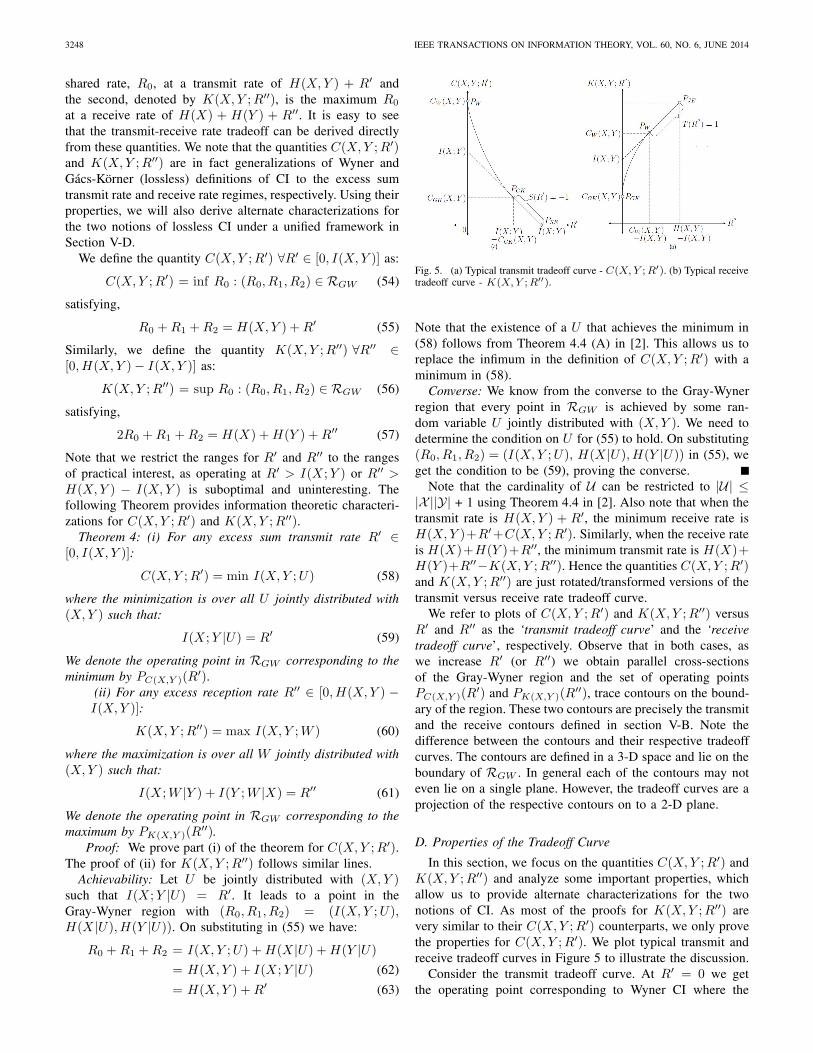
Fig. 5. (a) Typical transmit tradeoff curve - C(X, Y ; R′). (b) Typical receivetradeoff curve - K(X, Y ; R′′).

Note that the existence of a U that achieves the minimum in(58) follows from Theorem 4.4 (A) in [2]. This allows us toreplace the infimum in the definition of C(X, Y ; R′) with aminimum in (58).

Converse: We know from the converse to the Gray-Wynerregion that every point in RGW is achieved by some ran-dom variable U jointly distributed with (X, Y ). We need todetermine the condition on U for (55) to hold. On substituting(R0, R1, R2) = (I(X, Y ; U), H(X |U), H(Y |U)) in (55), weget the condition to be (59), proving the converse.

Note that the cardinality of U can be restricted to |U| ≤|X ||Y| + 1 using Theorem 4.4 in [2]. Also note that when thetransmit rate is H(X, Y ) + R′, the minimum receive rate isH(X, Y )+R′+C(X, Y ; R′). Similarly, when the receive rateis H(X)+H(Y )+R′′, the minimum transmit rate is H(X)+H(Y )+R′′−K(X, Y ; R′′). Hence the quantities C(X, Y ; R′)and K(X, Y ; R′′) are just rotated/transformed versions of thetransmit versus receive rate tradeoff curve.

We refer to plots of C(X, Y ; R′) and K(X, Y ; R′′) versusR′ and R′′ as the ‘transmit tradeoff curve’ and the ‘receivetradeoff curve’, respectively. Observe that in both cases, aswe increase R′ (or R′′) we obtain parallel cross-sectionsof the Gray-Wyner region and the set of operating pointsPC(X,Y )(R′) and PK(X,Y )(R′′), trace contours on the bound-ary of the region. These two contours are precisely the transmitand the receive contours defined in section V-B. Note thedifference between the contours and their respective tradeoffcurves. The contours are defined in a 3-D space and lie on theboundary of RGW . In general each of the contours may noteven lie on a single plane. However, the tradeoff curves are aprojection of the respective contours on to a 2-D plane.

D. Properties of the Tradeoff Curve

In this section, we focus on the quantities C(X, Y ; R′) andK(X, Y ; R′′) and analyze some important properties, whichallow us to provide alternate characterizations for the twonotions of CI. As most of the proofs for K(X, Y ; R′′) arevery similar to their C(X, Y ; R′) counterparts, we only provethe properties for C(X, Y ; R′). We plot typical transmit andreceive tradeoff curves in Figure 5 to illustrate the discussion.

Consider the transmit tradeoff curve. At R′ = 0 we getthe operating point corresponding to Wyner CI where the


minimum shared information is given by CW (X, Y ). Thispoint is denoted by PW in Figure 5. Next observe that atR0 = 0, for lossless reconstruction of X and Y , we need,R1 ≥ H(X) and R2 ≥ H(Y ). Therefore at an excess sumtransmit rate R′ = H(X)+H(Y )−H(X, Y ) = I(X ; Y ), theshared rate vanishes, or, C(X, Y ; I(X ; Y )) = 0. We call thispoint - ‘separate encoding’ and denote it by PSE in the figure.It is also obvious that any U independent of (X, Y ) achievesthis minimum R0 for R′ = I(X ; Y ).

Lemma 2 (Convexity): C(X, Y ; R′) is convex for R′ ∈[0, I(X ; Y )] and K(X, Y ; R′′) is concave for R′′ ∈[0, H(X, Y ) − I(X ; Y )].

Proof: The proof follows directly from the convexity ofthe Gray-Wyner region.Lemma 3 (Monotonicity 3): C(X, Y ; R′) is strictly monotonedecreasing ∀R′ ∈ [0, I(X ; Y )] and K(X, Y ; R′′) is strictlymonotone increasing ∀R′′ ∈ [0, H(X, Y ) − I(X ; Y )]

Proof: It is clear from the achievability results of Gray-Wyner that if a point (r0, r1, r2) ∈ RGW , then all points{(R0, R1, R2) : R0 ≥ r0, R1 ≥ r1, R2 ≥ r2} ∈ RGW . LetC(X, Y ; R′) = r0, for some excess transmission rate R′ andlet the corresponding operating point in RGW be (r0, r1, r2).Hence for any Δ > 0, the point (r0, r1 + Δ, r2) ∈ RGW andsatisfies R0 + R1 + R2 = R + Δ. Therefore,

C(X, Y ; R′ + Δ) = inf R0 : {R0 + R1 + R2 = R + Δ}≤ r0 (64)

Hence, C(X, Y ; R′) is non-increasing. Then it follows fromconvexity that C(X, Y ; R′) is either a constant or is strictlymonotone decreasing. Lemma 4 below eliminates the possi-bility of a constant, proving this lemma.

At all R′ where C(X, Y ; R′) is differentiable, we denotethe slope by S(R′). At non-differentiable points, we denote byS−(R′) and S+(R′) the left and right derivatives, respectively.Similarly the slope, left derivative and right derivatives ofK(X, Y ; R′′) are denoted by T (R′′), T−(R′′) and T +(R′′),respectively.

Lemma 2: The slope of C(X, Y ; R′), S(R′) ≤ −1 ∀R ∈[0, I(X ; Y )] where the curve is differentiable. At non-differentiable points, we have S−(R′) < S+(R′) ≤ −1.Similarly we have, T (R′′) ≥ 1 ∀R′′ ∈ [0, H(X, Y )−I(X ; Y )]and T−(R′′) > T +(R′′) ≥ 1

Proof: Note that it is sufficient for us to show thatS−(I(X ; Y )) ≤ −1. Then it directly follows from convexitythat S(R′) ≤ −1 at all differentiable points and S−(R′) <S+(R′) ≤ −1 at all non-differentiable points. Consider > 0, and fix the shared information rate to be R0 = .From the converse of the source coding theorem for losslessreconstruction, we have:

R0 + R1 = + R1 ≥ H(X)R0 + R2 = + R2 ≥ H(Y ) (65)

The above inequalities imply R0 + R1 + R2 ≥ H(X, Y ) +I(X ; Y ) − . Therefore the point on the transmit tradeoffcurve with C(X, Y ; R′) = has R′ ≥ I(X ; Y ) − . HenceS−(I(X ; Y )) ≤ −1 proving the Lemma.

Remark 3: Observe that the above proofs do not rely onthe lossless definitions of C(X, Y ; R′) and K(X, Y ; R′′), butleverage only on the convexity of the lossless Gray-Wynerregion. It is well known that the lossy Gray-Wyner region isalso convex in the rates, for all distortion pairs. Consequently,all the three lemmas (2, 3 and 4) can be easily extended tothe lossy counterparts of C(X, Y ; R′) and K(X, Y ; R′′). Weomit the details of the proof here to avoid repetition.

E. Alternate Characterizations for CGK(X, Y )and CW (X, Y )

In this section, we provide alternate characterizations forCGK(X, Y ) and CW (X, Y ) in terms of C(X, Y ; R′) andC(X, Y ; R′′), respectively.

Theorem 5: An alternate characterization for theGács-Körner CI is:

CGK(X, Y ) = supR′:S+(R′)=−1

C(X, Y ; R′) (66)

If there exists no R′ for which S+(R′) = −1, then,CGK(X, Y ) = 0. Similarly, an alternate characterization forWyner’s CI is :

CW (X, Y ) = infR′′:T+(R′′)=1

K(X, Y ; R′′) (67)

If there exists no R′′ for which T +(R) = 1, then,CW (X, Y ) = H(X, Y ). Note that CGK(X, Y ) corresponds tothat excess sum transmit rate where the region of C(X, Y ; R′)with slope < −1 meets the region with slope equal to −1, andCW (X, Y ) corresponds to that excess receive rate where theregion of K(X, Y ; R′′) with slope > 1 meets the region withslope equal to 1.

Proof: We first assume that there exists some R∗ ∈[0, I(X ; Y )), which is the minimum rate at which S+(R∗) =−1. We need to show that C(X, Y ; R∗) = CGK(X, Y ). Wedenote this point by PGK in the figure. Let R be such thatR∗ ≤ R < I(X ; Y ) and let U be the random variablewhich achieves the minimum shared information rate at Rin Theorem 4. Then it follows from Lemmas 2 and 4 thatS+(R) = −1. Then the point in the GW region correspondingto U satisfies the following two conditions:

R0 = I(X, Y ) − R

R0 + R1 + R2 = H(X, Y ) + R (68)

Adding the two equations, we have 2R0+R1+R2 = H(X)+H(Y ), which implies that R0 + R1 = H(X) and R0 + R2 =H(Y ). Therefore, the point corresponding to U satisfies Gács-Körner constraints (14). Hence, it follows that, any R such thatS+(R) = −1 leads to an operating point in the GW regionwhich satisfies Gács-Körner constraints.

Next, we need to show the converse. Consider any point inthe GW region satisfying Gács-Körner constraints. It can bewritten as,

R0 = I(X ; Y ) − R

R1 = H(X) − (I(X ; Y ) − R)R2 = H(Y ) − (I(X ; Y ) − R) (69)


for some CGK(X, Y ) ≤ R ≤ I(X ; Y ). On summing the threeequations, we have R0 + R1 + R2 = H(X, Y ) + R. It thenfollows from the convexity of C(X, Y ; R′) that S+(R) = −1.Therefore, we have,

C(X, Y ; R∗) = I(X ; Y ) − R∗

= I(X ; Y ) − minR:S+(R)=−1

R

= max{

R0 : (R0, R1, R2) ∈ RGW

R0 + R1 = H(X), R0 + R2 = H(Y )}

= CGK(X, Y ) (70)

proving the first part of the theorem. However, if there existsno R′ ∈ [0; I(X ; Y )] for which S+(R′) = −1, it implies that∀R′ ∈ [0; I(X ; Y )), C(X ; Y ; R′) > I(X ; Y ). Therefore (14)is not satisfied with equality for any R′ ∈ [0; I(X ; Y )). HenceCGK(X, Y ) = 0.

Note that the above characterizations for CGK(X, Y ) andCW (X, Y ) are of fundamentally different nature from theiroriginal characterizations and provide important insights intothe understanding of shared information. Moreover, from apractical standpoint, these characterizations also play a role infinding the minimum communication cost for networks whenthe cost of transmission on each link is a non-linear functionof the rate as illustrated in [4].

VI. CONCLUSION

In this paper we derived single letter information theoreticcharacterizations for the lossy generalizations of the two mostprevalent notions of CI due to Wyner and due to Gácsand Körner. These generalizations allow us to extend thetheoretical interpretation underlying their original definitionsto sources with infinite entropy (eg. continuous random vari-ables). We use these information theoretic characterizationsto derive the CI of bivariate Gaussian random variables. Wefinally showed that the operating points associated with thetwo notions of CI arise as extreme special cases of a broaderframework, that involves the tradeoff between the the totaltransmit versus the receive rate in the Gray-Wyner network.For the lossless setting, single letter information theoreticcharacterization for the tradeoff curve was established. Usingthe properties of the tradeoff curve, alternate characterizationsunder a common framework were derived for the two notionsof CI.

APPENDIX A

PROOF OF THEOREM 1 FOR THE GENERAL SETTING

In this appendix, we extend the proof of Theorem 1 forgeneral sources and distortion measures. Here, we do notassume that every point on the intersection of the Gray-Wyner region and the Pangloss plane satisfies (5) with equalityfor some joint density P (X, Y, U, X, Y ). We note that anequivalent definition of Wyner’s lossy CI is given by thefollowing. For any ε > 0, let Rmin

0 (D1, D2, ε) be definedas:

Rmin0 (D1, D2, ε) = inf R0 (71)

over all points (R0, R1, R2) satisfying:

(R0, R1, R2) ∈ RGW (D1, D2)R0 + R1 + R2 ≤ RX,Y (D1, D2) + ε (72)

Then,

CW (X, Y ; D1, D2) = limε→0

Rmin0 (D1, D2, ε) (73)

In the following Lemma, we derive upper and lower boundsto CW (X, Y ; D1, D2) in terms of ε.

Lemma 3: Let ε > 0 be given. Then, an upper bound toCW (X, Y ; D1, D2) is:

CW (X, Y ; D1, D2) ≤ inf I(X, Y ; U) (74)

where the infimum is over all joint densities P (X, Y, X, Y , U)satisfying:

I(X, Y ; X, Y ) ≤ RX,Y (D1, D2) + εI(X, Y ; U |X, Y ) = 0

I(X ; Y |U) = 0E(dX(X, X)) ≥ D1

E(dY (Y, Y )) ≥ D2 (75)

We denote this upper bound by CUBW (D1, D2, ε).

A lower bound to CW (X, Y ; D1, D2) is:

CW (X, Y ; D1, D2) ≥ inf I(X, Y ; U) (76)


I(X, Y ; X, Y ) ≤ RX,Y (D1, D2) + εI(X, Y ; U |X, Y ) ≤ ε

I(X ; Y |U) ≤ εE(dX(X, X)) ≥ D1

E(dY (Y, Y )) ≥ D2 (77)

We denote this lower bound by CLBW (D1, D2, ε).

Proof: The proof follows using very similar arguments tothat in the proof of Theorem 1. Hence, we omit the detailshere to avoid repetition.

Observe that the proof of Theorem 1 for the generalsetting follows once we show that CUB

W (D1, D2, ε) andCLB

W (D1, D2, ε) are continuous at ε = 0. The followingLemma sheds light on the the continuity of these quantities atε = 0.

Lemma 4: Let (D1, D2) be a pair of distortions at whichthere exists at least one distribution P (X, Y |X, Y ) that isRD-optimal in achieving RX,Y (D1, D2). Then:

CW (X, Y ; D1, D2) = CLBW (D1, D2, 0) = CUB

W (D1, D2, 0)(78)

However, if there exists no RD-optimal distribution, i.e.,there only exist distributions that can infinitesimally approachRX,Y (D1, D2), then:

CW (X, Y ; D1, D2) = limε→0

CLBW (D1, D2, ε)

= limε→0

CUBW (D1, D2, ε) (79)

Proof: To prove this Lemma, we employ techniquesvery similar to the ones used by Wyner in [2]. We further


restrict ourselves to discrete random variables for simplicity.However, the arguments can be easily extended to well-behaved continuous random variables and distortion measuresusing standard techniques.

We first show that the quantity CLBW (D1, D2, ε) is a convex

function of ε for all ε > 0. Towards proving this, define ageneralized version of CLB

W (D1, D2, ε) as:

CLBW (D1, D2, ε1, ε2, ε3) = inf I(X, Y ; U) (80)


I(X, Y ; X, Y ) ≤ RX,Y (D1, D2) + ε1

I(X, Y ; U |X, Y ) ≤ ε2

I(X; Y |U) ≤ ε3

E(dX(X, X)) ≥ D1

E(dY (Y, Y )) ≥ D2 (81)

Particularly, we show that CLBW (D1, D2, ε1, ε2, ε3) is con-

vex with respect to εi for any fixed values of εj and εk,i, j, k ∈ {1, 2, 3}.

Let ε2 > 0 and ε3 > 0 be fixed. Let ε11 > 0 and ε12 > 0 betwo values for ε1 and let the corresponding optimizing distrib-utions for (80) be P1(X, Y, X, Y , U) and P2(X, Y, X, Y , U),respectively. Now consider ε1 = θε11 + (1 − θ)ε12, for some0 < θ < 1. It is easy to check that the joint distribution thattakes value P1 with probability θ and value P2 with probability1 − θ, denoted hereafter by Pθ , satisfies all the constraints in(81) for ε1,ε2 and ε3. Next, consider the following series ofinequalities:

CLBW (D1, D2, ε1, ε2, ε3)

≤ IPθ (X, Y ; U)= θIP1(X, Y ; U) + (1 − θ)IP2(X, Y ; U)= θCLB

W (D1, D2, ε11, ε2, ε3)+(1 − θ)CLB

W (D1, D2, ε12, ε2, ε3)

where IP (·, ·) denotes the mutual information withrespect to joint density P . This proves convexity ofCLB

W (D1, D2, ε1, ε2, ε3) with respect to ε1 for fixed ε2and ε3. Similar arguments lead to the conclusion thatCLB

W (D1, D2, ε1, ε2, ε3) is convex with respect to (ε1, ε2, ε3)when ε1 > 0, ε2 > 0 and ε3 > 0. Hence, CLB

W (D1, D2, ε)and CUB

W (D1, D2, ε) are convex and continuous for all ε > 0.To prove that CLB

W (D1, D2, ε1, ε2, ε3) is continuous atthe origin, we first consider continuity with respect toε2 for fixed ε1 and ε3. Let ε1, ε2, ε3 > 0 and letP (X, Y, X, Y , U) be the joint density that achieves the opti-mum for CLB

W (D1, D2, ε1, ε2, ε3). It is sufficient for us toprove that there exists a joint density Q(X, Y, X, Y , U) thatsatisfies (81) with ε2 = 0, and for which IQ(X, Y ; U) iswithin δ(ε2) from CLB

W (D1, D2, ε1, ε2, ε3), for some δ(ε2) →0 as ε2 → 0. We construct the joint density Q(·) as follows:

Q(X, Y, X, Y , U) = P (X, Y )P (X, Y |X, Y )P (U |X, Y )

Observe that all the conditions in (81) with ε2 = 0 are satisfiedby Q(·), as IQ(X, Y ; U |X, Y ) = 0. We need to show that

|IP (X, Y ; U)− IQ(X, Y ; U)| ≤ δ(ε2) for some δ(ε2) → 0 asε2 → 0. Towards proving this result, we have:

ε2 = IP (X, Y ; U |X, Y )≥(a) sup |P (X, Y, U |X, Y ) − Q(X, Y, U |X, Y )|

where (a) follows from Pinsker’s inequality [21] and thesupremum is over all possible subsets of alphabets of(X, Y, U, X, Y ). The above inequalities state that the jointdensities P (X, Y, X, Y , U) and Q(X, Y, X, Y , U) have a totalvariation smaller than ε2. Therefore, as ε2 → 0, P (·) →Q(·). As conditional entropy is continuous in the total vari-ation distance of the corresponding random variables, thereexists a δ(ε2) such that |IP (X, Y ; U) − IQ(X, Y ; U)| ≤δ(ε2) and δ(ε2) → 0 as ε2 → 0. This proves thatlimε2→0 CLB

W (D1, D2, ε1, ε2, ε3) = CLBW (D1, D2, ε1, 0, ε3).

The proof for continuity with respect to ε3 at origin followsin very similar lines to the proof of [2, Th. 4.4]. Hence, weomit the details here. This leads to the conclusion that:

CW (X, Y ; D1, D2) = limε→0

CLBW (D1, D2, ε)

= limε→0

CUBW (D1, D2, ε)

The proof of this Lemma follows directly by observing that,if there exists a joint density P (X, Y |X, Y ) that achievesRX,Y (D1, D2), then both the above limits converge toCUB

W (D1, D2, 0), which is same as the information theoreticcharacterization in (18).

APPENDIX B

PROOF OF COROLLARY 1

Proof: Our objective is to prove that the optimizingdistribution in Theorem 1 satisfies (27). We begin with anauxiliary property of the RD-optimal conditional distributionP (X∗, Y ∗|X, Y ). Recall that the RD optimal conditionaldistribution minimizes I(X, Y ; X∗, Y ∗) over all joint distrib-utions that satisfy the distortion constraints, E(dX(X, X∗)) ≤D1 and E(dY (Y, Y ∗)) ≤ D2. Hence, it follows using standardarguments [11] that, for every distortion pair (D1, D2), theRD-optimal conditional distribution, P (X∗, Y ∗|X, Y ), alsominimizes the following Lagrangian for some positive con-stants μ1, μ2 and positive valued function λ(x, y) defined forall x ∈ X ,y ∈ Y:

L = I(X, Y ; X∗, Y ∗)−μ1E(dX(X, X∗)) − μ2E(dY (Y, Y ∗))

−ˆ

λ(x, y)dxdy

ˆdx∗dy∗P (x∗, y∗|x, y) (82)

Upon differentiating the above Lagrangian with respect toP (x∗, y∗|x, y) and setting it to zero leads to the necessaryconditions for optimality of the joint distribution. Some routinesteps and simplifications lead to the conclusion that the jointdistribution P (X, Y, X∗, Y ∗) must satisfy the following:

P (X∗, Y ∗|X, Y ) = λ(X, Y )P (X∗, Y ∗)× exp(dX(X, X∗)) exp(dY (Y, Y ∗)) (83)


It follows that the conditional density P (X, Y |X∗, Y ∗)satisfies:

P (X,Y |X∗, Y ∗)=φ(X,Y )exp(dX(X, X∗))exp(dY (Y, Y ∗))(84)

where φ(X, Y ) = λ(X, Y )P (X, Y ).Next recall that the optimizing distribution in Theorem 1

satisfies the following two Markov conditions:

(X, Y ) ↔ (X∗, Y ∗) ↔ U

X∗ ↔ U ↔ Y ∗ (85)

Hence the optimizing joint distribution can be rewritten as:

P (X, Y, X∗, Y ∗, U) = P (U)P (X∗|U)P (Y ∗|U)×P (X, Y |X∗, Y ∗)

= φ1(X, X∗, U)φ2(Y, Y ∗, U)φ(X, Y )(86)

where φ1(X, X∗, U) = P (U)P (X∗|U) exp(dX(X, X∗)) andφ2(Y, Y ∗, U) = P (Y ∗|U) exp(dY (Y, Y ∗)). Hence, it followsthat:

P (X∗, Y ∗, U |X, Y ) = φ1(X, X∗, U)φ2(Y, Y ∗, U)λ(X, Y )(87)

which implies that the Markov conditions in (27) must besatisfied, proving the Lemma.

APPENDIX C

SHANNON LOWER BOUND FOR VECTORS

In this appendix, we review some of the definitions andresults pertinent to Shannon lower bounds for vectors ofrandom variables. We refer to [11] (section 4.3.1) for furtherdetails on Shannon lower bound and its properties.

Let X be an n-dimensional random variable distributedaccording to p(X), and let ρi(xi, xi) ∀i ∈ {1, . . . , N} be anywell defined difference distortion measures, i.e., ρi(x, x) =ρi(x − x). Let RX(D) be the rate-distortion function of X,with respect to the given distortion measures, i.e.:

RX(D) = infP (X|X):E[ρi(xi,xi)]≤Di ∀i

I(X, X) (88)

Then the Shannon lower bound to RX(D), denoted byRL

X(D), is given by:

RLX(D) = H(X)

− sups1,...,sn<0

N∑

i=1

{siDi − log

ˆesiρi(zi)dzi

}

= H(X) −N∑

i=1

maxgi∈Gi(Di)

H(gi) (89)

where, Gi(Di) denotes the set of all joint distributions suchthat: ˆ

ρi(zi)g(zi)dzi ≤ Di (90)

The above derivation is a direct extension of the derivation inSection 4.3.1 in [11], to vectors of random variables. It is easyto verify that the distribution gi that achieves the maximumin (89) is given by:

gi(z) =esiρ(z)´esiρ(z)dz

(91)

where, si is such that:ˆgi(z)ρi(z)dz = Di (92)

Shannon showed that RLX(D) ≤ RX(D) always holds

(see [11] for details). The following lemma states the necessaryand sufficient conditions for RL

X(D) = RX(D).Lemma 5: RL

X(D) = RX(D) iff the distribution of X canbe expressed as:

p(x) =ˆ

q(x)n∏

i

gi(xi − xi)dx (93)

i.e., X can be expressed as the sum of two statisticallyindependent random vectors, X and Z, where Z is distributedaccording to:

g(Z) =n∏

i

gi(zi) (94)

where gi(z) is given by (91).Proof: Direct extension of [11, Th. 4.3.1].

It follows from the above Lemma that, if Shannon lowerbound is tight, X is the RD-optimal reconstruction and theRD-optimal backward channel from X to X is additive andcan be written as:

X = X + Z (95)

where Z ∼∏ni gi(Zi). Therefore, if Shannon lower bound is

tight, the components of X are independent given X, i.e., thejoint density p(X, X) is of the form:

p(X, X) = q(X)n∏

i

pi(Xi|Xi). (96)

REFERENCES

[1] P. Gács and J. Körner, “Common information is far less than mutualinformation,” Problems Control Inf. Theory, vol. 2, no. 2, pp. 149–162,1973.

[2] A. Wyner, “The common information of two dependent random vari-ables,” IEEE Trans. Inf. Theory, vol. 21, no. 2, pp. 163–179, Mar. 1975.

[3] R. Gray and A. Wyner, “Source coding for a simple network,” Bell Syst.Tech. J., vol. 53, pp. 1681–1721, Nov. 1974.

[4] K. Viswanatha, E. Akyol, and K. Rose, “An optimal transmit-receiverate tradeoff in Gray-Wyner network and its relation to common infor-mation,” in Proc. IEEE ITW, Oct. 2011, pp. 105–109.

[5] S. Kamath and V. Anantharam, “A new dual to the Gács-Körner commoninformation defined via the Gray-Wyner system,” in Proc. 48th Annu.Allerton Conf. Commun., Control, Comput., Oct. 2010, pp. 1340–1346.

[6] H. Yamamoto, “Coding theorems for Shannon’s cipher system withcorrelated source outputs, and common information,” IEEE Trans. Inf.Theory, vol. 40, no. 1, pp. 85–95, Jan. 1994.

[7] G. Xu, W. Liu, and B. Chen, “Wyner’s common information forcontinuous random variables—A lossy source coding interpretation,” inProc. 45th Annu. Conf. CISS, 2011, pp. 1–6.


[8] K. Viswanatha, E. Akyol, and K. Rose, “Lossy common informationof two dependent random variables,” in Proc. IEEE ISIT, Jul. 2012,pp. 528–532.

[9] R. Ahlswede and J. Körner, “On common information and relatedcharacteristics of correlated information sources,” in Proc. 7th PragueConf. Inf. Theory, 1974.

[10] R. Venkataramani, G. Kramer, and V. Goyal, “Multiple descriptioncoding with many channels,” IEEE Trans. Inf. Theory, vol. 49, no. 9,pp. 2106–2114, Sep. 2003.

[11] T. Berger, Rate Distortion Theory. Englewood Cliffs, NJ, USA:Prentice-Hall, 1971.

[12] R. Gray, “A new class of lower bounds to information rates of stationarysources via conditional rate-distortion functions,” IEEE Trans. Inf.Theory, vol. 19, no. 4, pp. 480–489, Jul. 1973.

[13] J. Nayak, E. Tuncel, D. Gunduz, and E. Erkip, “Successive refinementof vector sources under individual distortion criteria,” IEEE Trans. Inf.Theory, vol. 56, no. 4, pp. 1769–1781, Apr. 2010.

[14] Y. Wu and S. Verdu, “Functional properties of minimum mean-squareerror and mutual information,” IEEE Trans. Inf. Theory, vol. 58, no. 3,pp. 1289–1301, Mar. 2012.

[15] R. Zamir, “A proof of the Fisher information inequality via a dataprocessing argument,” IEEE Trans. Inf. Theory, vol. 44, no. 3,pp. 1246–1250, May 1998.

[16] K. Viswanatha, E. Akyol, T. Nanjundaswamy, and K. Rose, “On com-mon information and the encoding of sources that are not successivelyrefinable,” in Proc. IEEE ITW, Sep. 2012, pp. 129–133.

[17] D. Marco and M. Effros, “On lossless coding with coded side informa-tion,” IEEE Trans. Inf. Theory, vol. 55, no. 7, pp. 3284–3296, Jul. 2009.

[18] P. Cuff, “Communication requirements for generating correlated ran-dom variables,” in Proc. IEEE Int. Symp. Inf. Theory, Jul. 2008,pp. 1393–1397.

[19] J. Nayak, S. Ramaswamy, and K. Rose, “Correlated source coding forfusion storage and selective retrieval,” in Proc. IEEE Int. Symp. Inf.Theory, Sep. 2005, pp. 92–96.

[20] K. Viswanatha, E. Akyol, and K. Rose, “On optimum communicationcost for joint compression and dispersive information routing,” in Proc.IEEE ITW, Sep. 2010, pp. 1–5.

[21] T. Cover and J. Thomas, Elements of Information Theory. New York,NY, USA: Wiley, 1991.

Kumar B. Viswanatha (S’08) received his PhD degree in 2013 in the Elec-trical and Computer Engineering department from University of California atSanta Barbara (UCSB), USA. He is currently working for Qualcomm researchcenter in San Diego. Prior to joining Qualcomm, he was an intern associate inthe equity volatility desk at Goldman Sachs Co., New York, USA. His researchinterests include multi-user information theory, wireless communications, jointcompression and routing for networks and distributed compression for largescale sensor networks.

Emrah Akyol (S’03–M’12) received the Ph.D. degree in 2011 in electricaland computer engineering from the University of California at Santa Barbara.From 2006 to 2007, he held positions at Hewlett-Packard Laboratories andNTT Docomo Laboratories, both in Palo Alto, where he worked on topics invideo compression.

Currently, Dr. Akyol is a postdoctoral researcher in the Electrical Engineer-ing Department, University of Southern California. His current research is onthe interplay of networked information theory, communications and control.

Kenneth Rose (S’85–M’91–SM’01–F’03) received the Ph.D. degree in 1991from the California Institute of Technology, Pasadena.

He then joined the Department of Electrical and Computer Engineering,University of California at Santa Barbara, where he is currently a Professor.His main research activities are in the areas of information theory and signalprocessing, and include rate-distortion theory, source and source-channelcoding, audio and video coding and networking, pattern recognition, andnonconvex optimization. He is interested in the relations between informationtheory, estimation theory, and statistical physics, and their potential impact onfundamental and practical problems in diverse disciplines.

Dr. Rose was co-recipient of the 1990 William R. Bennett Prize PaperAward of the IEEE Communications Society, as well as the 2004 and 2007IEEE Signal Processing Society Best Paper Awards.

Documents

3238 IEEE TRANSACTIONS ON INFORMATION THEORY… · 3238 IEEE TRANSACTIONS ON INFORMATION THEORY, VOL. 60, NO. 6, JUNE 2014 The Lossy Common Information of Correlated Sources Kumar