31545 Medical Imaging systems

Lecture 2: Ultrasound physics

Jørgen Arendt Jensen

Center for Fast Ultrasound Imaging

Section for Ultrasound and Biomechanics

Department of Health Technology

Technical University of Denmark

September 2, 2021

1

Outline of today

1. Discussion assignment on B-mode imaging

2. Signal processing quiz

3. Derivation of wave equation and role of speed of sound

4. Wave types and properties

5. Intensities and safety limits

6. Scattering of ultrasound

7. Questions for exercise 1 and practical details

2

Design an ultrasound B-mode system

Assume that a system can penetrate 300 wavelengths

It should penetrate down to 10 cm in a liver

1. What is the largest pulse repetition frequency possible?

2. What is the highest possible transducer center frequency?

3. What is the axial resolution?

4. What is the lateral resolution for an F-number of 2?

3

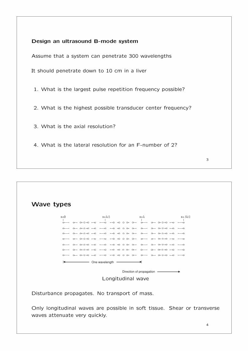
Wave types

One wavelength

Direction of propagation

λ/2x= λx= 3λ/2x=x=0

Longitudinal wave

Disturbance propagates. No transport of mass.

Only longitudinal waves are possible in soft tissue. Shear or transverse

waves attenuate very quickly.

4

Derivation of the wave equation in one dimension

5

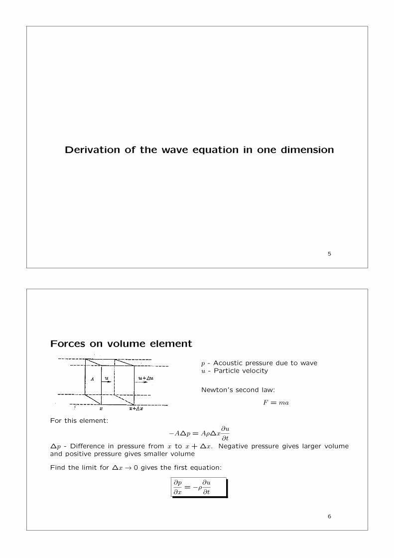
Forces on volume element

p - Acoustic pressure due to waveu - Particle velocity

Newton’s second law:

F = ma

For this element:

−A∆p = Aρ∆x∂u

∂t∆p - Difference in pressure from x to x + ∆x. Negative pressure gives larger volumeand positive pressure gives smaller volume

Find the limit for ∆x→ 0 gives the first equation:

∂p

∂x= −ρ∂u

∂t

6

Preservation of mass

Change in volume due to change in particle velocity:

∆vol = A∆u∆t

Assume linear relation to pressure

∆vol = −κ(A∆x)∆p

κ - Compressibility of material in [m2/N]

If the pressure on the volume is positive, then the volume gets smaller and the volumechange is negative.

Combined:

A∆u∆t = −κ(A∆x)∆p

After limit gives the second equation:

∂u

∂x= −κ∂p

∂t

7

Combining the two equations:

∂p

∂x= −ρ∂u

∂t

∂u

∂x= −κ∂p

∂t

Apply ∂/∂t on second eqn.:

∂ ∂u∂x

∂t=

∂2u

∂x∂t= −κ∂

2p

∂t2

Apply ∂/∂x on first eqn.:

∂2p

∂x2= −ρ

∂ ∂u∂t

∂x⇒ ∂2u

∂t∂x= −1

ρ

∂2p

∂x2

Combining gives:

−κ∂2p

∂t2= −1

ρ

∂2p

∂x2

leading to

∂2p

∂x2− ρκ∂

2p

∂t2= 0

8

The linear wave equation:

Introduce the speed of sound c:

c =

√1

ρκ

Finally gives the linear wave equation:

∂2p

∂x2− 1

c2∂2p

∂t2= 0

9

Solutions to the wave equation

Assume harmonic solution:

p(t, x) = p0 sin(ω0(t− x

c))

Insert into equation:

∂2p

∂x2− 1

c2

∂2p

∂t2= 0

(−p0

(ω0

c

)2+ p0

1

c2ω2

0) sin(ω0(t− x

c)) = 0

which shows this is a solution.

Note that c is speed of sound, which links spatial position and time.

General solutions:

p(t, x) = g(t± x

c)

x

cis time delay

10

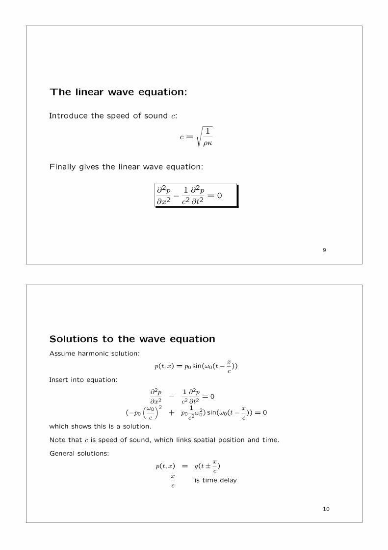
Link between speed of sound and delay

0 0.2 0.4 0.6 0.8 1 1.2 1.4 1.6 1.8

x 10−6

−1

0

1

2g(t−x/c) for x = 0

Norm

aliz

ed p

ressure

0 0.2 0.4 0.6 0.8 1 1.2 1.4 1.6 1.8

x 10−6

−1

0

1

2g(t−x/c) for x = 1.54 mm

x/c

Time [s]

Norm

aliz

ed p

ressure

Propagation of 2 cycle 5 MHz pulse in a medium with a speed of sound

of 1540 m/s.

11

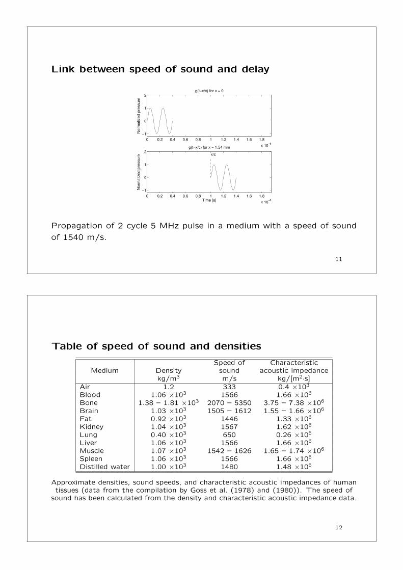
Table of speed of sound and densities

Speed of CharacteristicMedium Density sound acoustic impedance

kg/m3 m/s kg/[m2·s]Air 1.2 333 0.4 ×103

Blood 1.06 ×103 1566 1.66 ×106

Bone 1.38 – 1.81 ×103 2070 – 5350 3.75 – 7.38 ×106

Brain 1.03 ×103 1505 – 1612 1.55 – 1.66 ×106

Fat 0.92 ×103 1446 1.33 ×106

Kidney 1.04 ×103 1567 1.62 ×106

Lung 0.40 ×103 650 0.26 ×106

Liver 1.06 ×103 1566 1.66 ×106

Muscle 1.07 ×103 1542 – 1626 1.65 – 1.74 ×106

Spleen 1.06 ×103 1566 1.66 ×106

Distilled water 1.00 ×103 1480 1.48 ×106

Approximate densities, sound speeds, and characteristic acoustic impedances of humantissues (data from the compilation by Goss et al. (1978) and (1980)). The speed of

sound has been calculated from the density and characteristic acoustic impedance data.

12

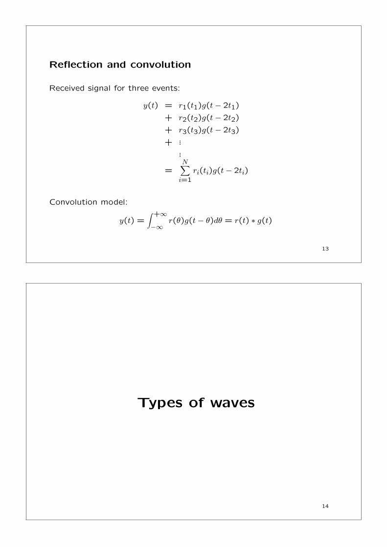
Reflection and convolution

Received signal for three events:

y(t) = r1(t1)g(t− 2t1)

+ r2(t2)g(t− 2t2)

+ r3(t3)g(t− 2t3)

+ ......

=N∑

i=1

ri(ti)g(t− 2ti)

Convolution model:

y(t) =∫ +∞

−∞r(θ)g(t− θ)dθ = r(t) ∗ g(t)

13

Types of waves

14

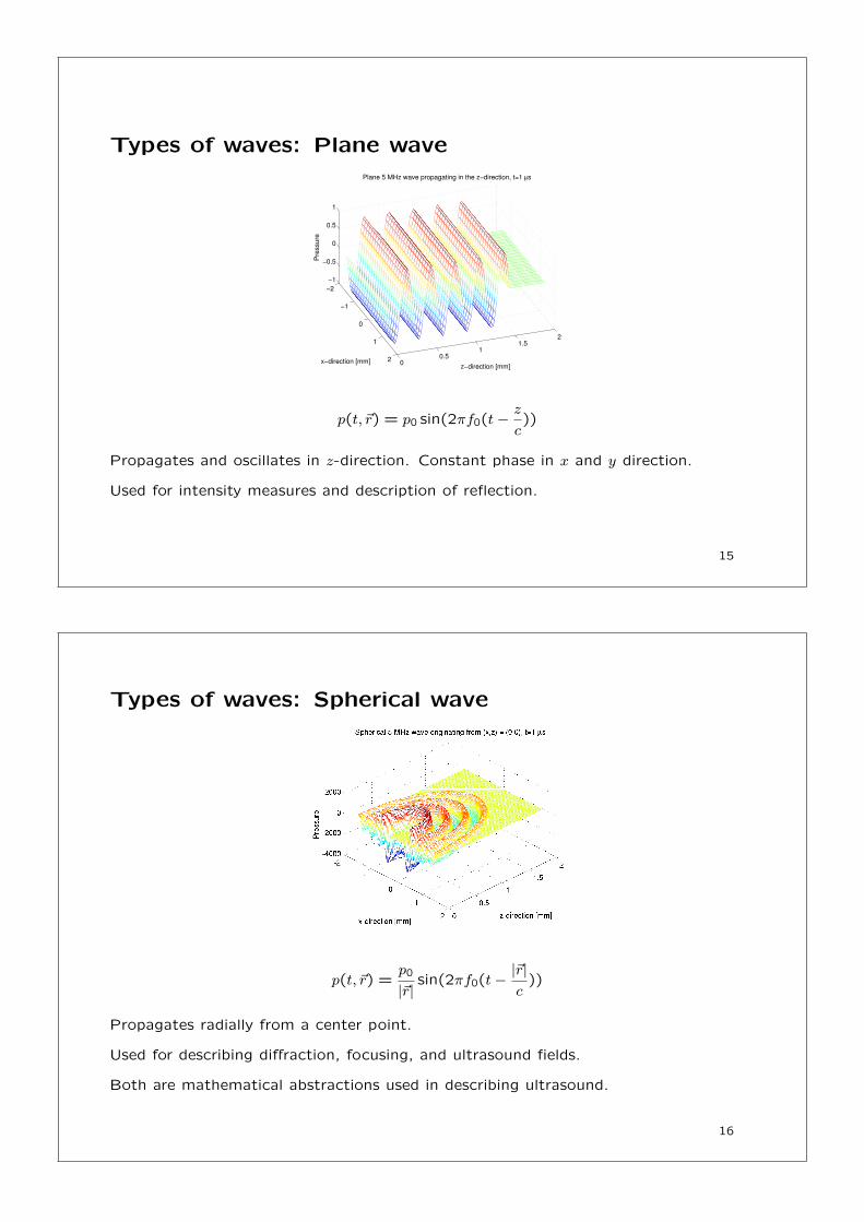
Types of waves: Plane wave

−2

−1

0

1

20

0.51

1.52

−1

−0.5

0

0.5

1

z−direction [mm]

Plane 5 MHz wave propagating in the z−direction, t=1 µs

x−direction [mm]

Pre

ssure

p(t, ~r) = p0 sin(2πf0(t− z

c))

Propagates and oscillates in z-direction. Constant phase in x and y direction.

Used for intensity measures and description of reflection.

15

Types of waves: Spherical wave

p(t, ~r) =p0

|~r| sin(2πf0(t− |~r|c

))

Propagates radially from a center point.

Used for describing diffraction, focusing, and ultrasound fields.

Both are mathematical abstractions used in describing ultrasound.

16

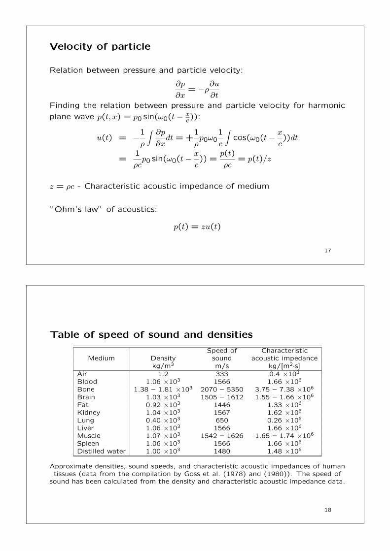
Velocity of particle

Relation between pressure and particle velocity:

∂p

∂x= −ρ∂u

∂t

Finding the relation between pressure and particle velocity for harmonic

plane wave p(t, x) = p0 sin(ω0(t− xc)):

u(t) = −1

ρ

∫∂p

∂xdt = +

1

ρp0ω0

1

c

∫cos(ω0(t− x

c))dt

=1

ρcp0 sin(ω0(t− x

c)) =

p(t)

ρc= p(t)/z

z = ρc - Characteristic acoustic impedance of medium

”Ohm’s law” of acoustics:

p(t) = zu(t)

17

Table of speed of sound and densities

Speed of CharacteristicMedium Density sound acoustic impedance

kg/m3 m/s kg/[m2·s]Air 1.2 333 0.4 ×103

Blood 1.06 ×103 1566 1.66 ×106

Bone 1.38 – 1.81 ×103 2070 – 5350 3.75 – 7.38 ×106

Brain 1.03 ×103 1505 – 1612 1.55 – 1.66 ×106

Fat 0.92 ×103 1446 1.33 ×106

Kidney 1.04 ×103 1567 1.62 ×106

Lung 0.40 ×103 650 0.26 ×106

Liver 1.06 ×103 1566 1.66 ×106

Muscle 1.07 ×103 1542 – 1626 1.65 – 1.74 ×106

Spleen 1.06 ×103 1566 1.66 ×106

Distilled water 1.00 ×103 1480 1.48 ×106

Approximate densities, sound speeds, and characteristic acoustic impedances of humantissues (data from the compilation by Goss et al. (1978) and (1980)). The speed of

sound has been calculated from the density and characteristic acoustic impedance data.

18

Example

Typical values: c = 1500 m/s, ρ = 1000 kg/m3

z = 1.5 · 106 kg/[M2 s] = 1.5 MRayl

p0 = 100 kPa, ω0 = 2π · 5 · 106 rad/s

gives

u =100 · 103

1.5 · 106= 0.06 m/s

Displacement:∫u(t)dt =

u

ω0= 2.1 nm

Actual particle displacements are very, very small.

19

Safety and intensity of ultrasound

20

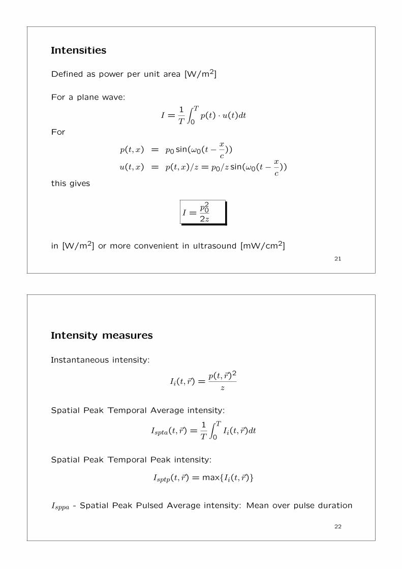
Intensities

Defined as power per unit area [W/m2]

For a plane wave:

I =1

T

∫ T0p(t) · u(t)dt

For

p(t, x) = p0 sin(ω0(t− xc

))

u(t, x) = p(t, x)/z = p0/z sin(ω0(t− xc

))

this gives

I =p2

0

2z

in [W/m2] or more convenient in ultrasound [mW/cm2]

21

Intensity measures

Instantaneous intensity:

Ii(t, ~r) =p(t, ~r)2

z

Spatial Peak Temporal Average intensity:

Ispta(t, ~r) =1

T

∫ T0Ii(t, ~r)dt

Spatial Peak Temporal Peak intensity:

Isptp(t, ~r) = max{Ii(t, ~r)}

Isppa - Spatial Peak Pulsed Average intensity: Mean over pulse duration

22

Example of intensities

0 0.5 1 1.5 2 2.5 3 3.5

x 10−5

0

0.2

0.4

0.6

0.8

1

Time [s]

Insta

nta

neous inte

nsity [W

/m ]

2

Isptp

Ispta

Isppa Isppa

Different measures of intensity for a typical ultrasound pulse. The pulse

repetition time is set artificially low at 17.5 µs.

23

FDA safety limits

Ispta.3 Isppa.3 ImmW/cm2 W/cm2 W/cm2 MI

Use In Situ Water In Situ Water In Situ WaterCardiac 430 730 190 240 160 600 1.90Peripheral vessel 720 1500 190 240 160 600 1.90Ophthalmic 17 68 28 110 50 200 0.23Fetal imaging (a) 94 170 190 240 160 600 1.90

Highest known acoustic field emissions for commercial scanners as stated by theUnited States FDA (The use marked (a) also includes intensities for abdominal,

intra-operative, pediatric, and small organ (breast, thyroid, testes, neonatal cephalic,and adult cephalic) scanning) from the the September 9, 2008, FDA Guidance.

24

Mechanical Index MI

Definition:

MI =pr.3(zsp)√

fc

Variables:

pr.3 - Peak negative pressure in MPa derated by 0.3 dB([MHz cm]

zsp - Point on the beam axis with the maximum pulse intensity integral

fc - Center frequency in MHz

25

Example

Plane wave with an intensity of 730 mW/cm2 (cardiac, water)

Pulse emitted: f0 = 5 MHz, M = 2 periods, Tprf = 200µs

Pressure emitted:

Ispta =1

Tprf

∫ M/f0

0Ii(t, ~r)dt =

M/f0

Tprf

P20

2z

p0 =

√√√√Ispta2zTprfM/f0

= 3.35 · 106 Pa = 33.5 atm

(Rock concert at 120 dB (pain level) is 50 Pa)

The normal atmospheric pressure is 100 kPa.

26

Example continued

The particle velocity is U0 = p0Z = 3.35·106

1.48·106 = 2.18 m/s.

The particle velocity is the derivative of the particle displacement, so

z(t) =∫U0 sin(ω0t− kz)dt =

U0

ω0cos(ω0t− kz).

The displacement is

z0 = U0/ω0 = 2.18/(2π · 5 · 106) = 69 nm.

Mechnical Index MI is without deration

MI =pr.3(zsp)√

fc=

3.35√5

= 1.5

at 7 cm with deration it is: 3.35·10−0.3·7·5/20√5

= 0.44

27

Typical intensities for fetal scanning in water

0 10 20 30 40 50 60 70 80 90 1000

50

100

150

200

Axial distance [mm]

Inte

nsity:

Isp

ta

[mW

/cm

2]

Focus at 60 mm, elevation focus at 40 mm (Fetal)

0 10 20 30 40 50 60 70 80 90 1000.5

1

1.5

2

2.5

Axial distance [mm]

Pe

ak p

ressu

re [

MP

a]

Simulated intensity profile in water for fetal scanning using a using a 65

elements 5 MHz linear array focused at 60 mm with an elevation focus

at 40 mm.

28

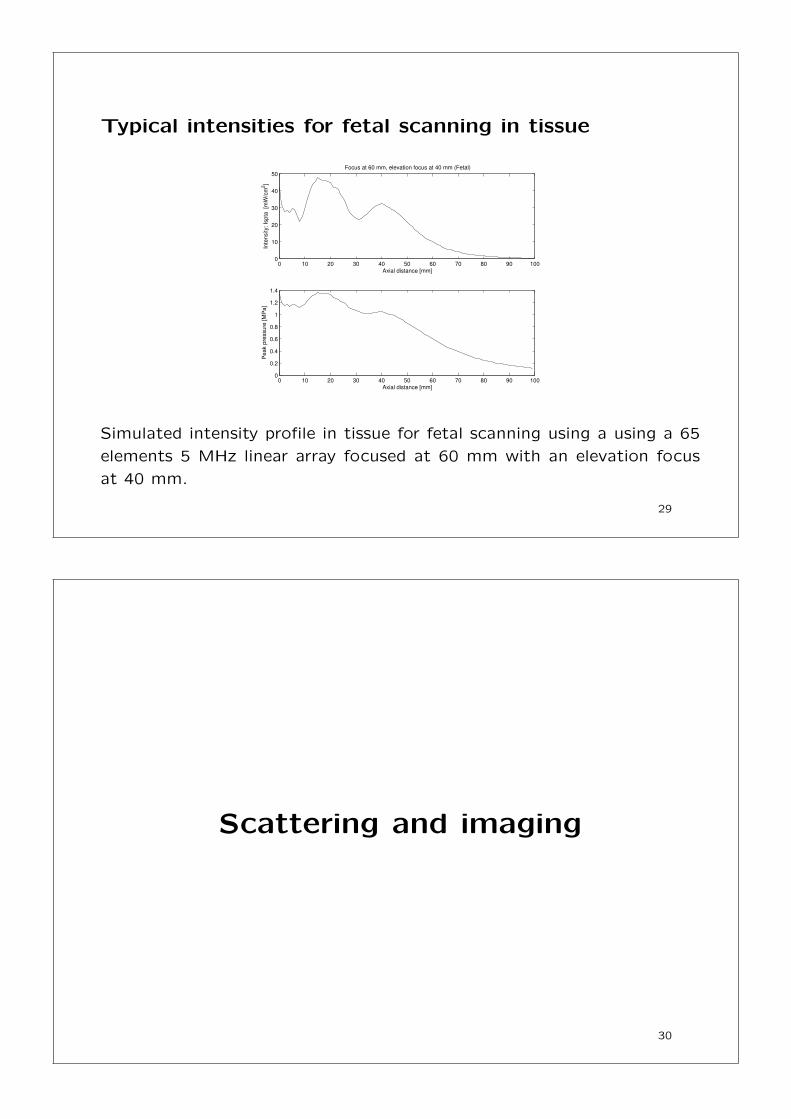
Typical intensities for fetal scanning in tissue

0 10 20 30 40 50 60 70 80 90 1000

10

20

30

40

50

Axial distance [mm]

Inte

nsity:

Isp

ta

[mW

/cm

2]

Focus at 60 mm, elevation focus at 40 mm (Fetal)

0 10 20 30 40 50 60 70 80 90 1000

0.2

0.4

0.6

0.8

1

1.2

1.4

Axial distance [mm]

Pe

ak p

ressu

re [

MP

a]

Simulated intensity profile in tissue for fetal scanning using a using a 65

elements 5 MHz linear array focused at 60 mm with an elevation focus

at 40 mm.

29

Scattering and imaging

30

Fetus

Amniotic fluid

Head

Mouth

Spine

Boundary of placenta

Amniotic fluid

Foot

Ultrasound image of 13th week fetus. The markers at the border of the

image indicate one centimeter.

31

Speckle pattern in ultrasound image

4 x 4 cm image of a human liver for a 28-year old male.

Speckle pattern in liver. The dark areas are blood vessels.

32

Backscattering

Power of backscattered signal:

Ps = Iiσsc

Ii - Incident intensity [W/m2]

σsc - Backscattering cross-section [m2]

Received power of backscattered signal at transducer:

Pr = Iiσscr2

4R2

r - Transducer radius

R - Distance to scattering region

33

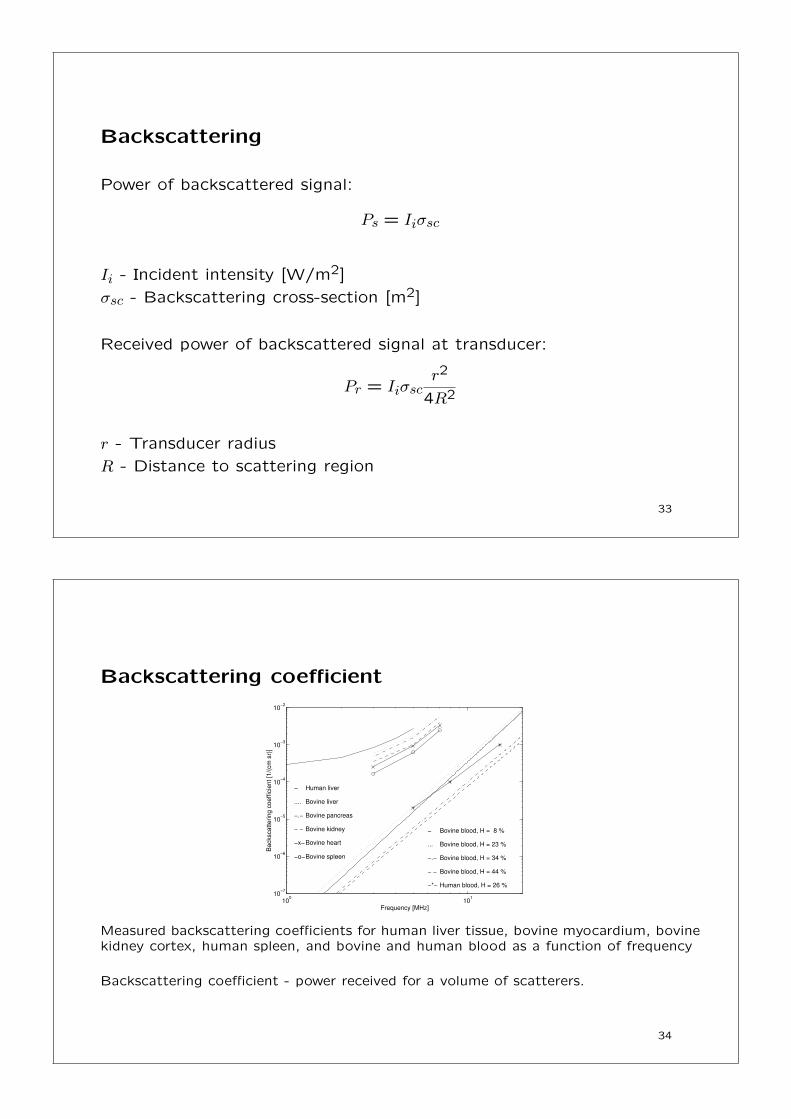
Backscattering coefficient

100

101

10−7

10−6

10−5

10−4

10−3

10−2

Frequency [MHz]

Ba

cksca

tte

rin

g c

oe

ffic

ien

t [1

/(cm

sr)

]

− Bovine blood, H = 8 %

... Bovine blood, H = 23 %

−.− Bovine blood, H = 34 %

− − Bovine blood, H = 44 %

−*− Human blood, H = 26 %

− Human liver

.... Bovine liver

−.− Bovine pancreas

− − Bovine kidney

−x−Bovine heart

−o−Bovine spleen

Measured backscattering coefficients for human liver tissue, bovine myocardium, bovinekidney cortex, human spleen, and bovine and human blood as a function of frequency

Backscattering coefficient - power received for a volume of scatterers.

34

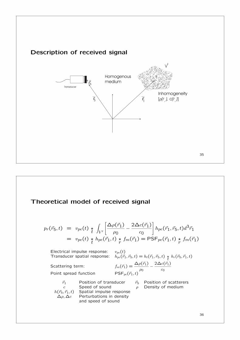
Description of received signal

35

Theoretical model of received signal

pr(~r5, t) = vpe(t) ?t

∫

V ′

[∆ρ(~r1)

ρ0− 2∆c(~r1)

c0

]hpe(~r1, ~r5, t)d

3~r1

= vpe(t) ?thpe(~r1, t) ?r

fm(~r1) = PSFpe(~r1, t) ?rfm(~r1)

Electrical impulse response: vpe(t)Transducer spatial response: hpe(~r1, ~r5, t) = ht(~r1, ~r5, t) ?

thr(~r5, ~r1, t)

Scattering term: fm(~r1) =∆ρ(~r1)

ρ0− 2∆c(~r1)

c0Point spread function PSFpe(~r1, t)

~r1 Position of transducer ~r5 Position of scatterersc Speed of sound ρ Density of medium

h(~r5, ~r1, t) Spatial impulse response∆ρ,∆c Perturbations in density

and speed of sound

36

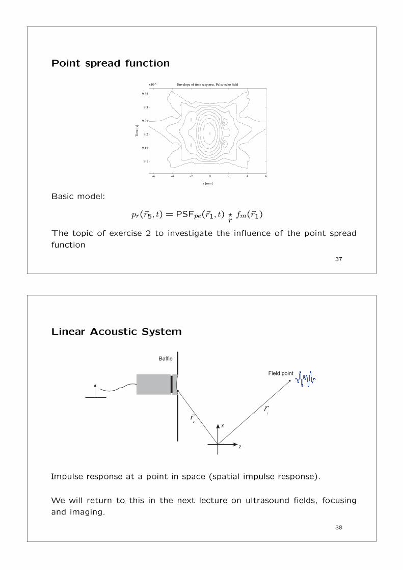
Point spread function

9.1

9.15

9.2

9.25

9.3

9.35

x10-5

-6 -4 -2 0 2 4 6

Envelope of time response, Pulse-echo field

x [mm]

Tim

e [s

]

Basic model:

pr(~r5, t) = PSFpe(~r1, t) ?rfm(~r1)

The topic of exercise 2 to investigate the influence of the point spread

function

37

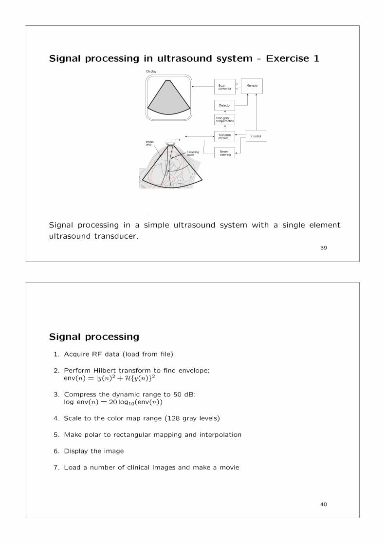
Linear Acoustic System

Impulse response at a point in space (spatial impulse response).

We will return to this in the next lecture on ultrasound fields, focusing

and imaging.

38

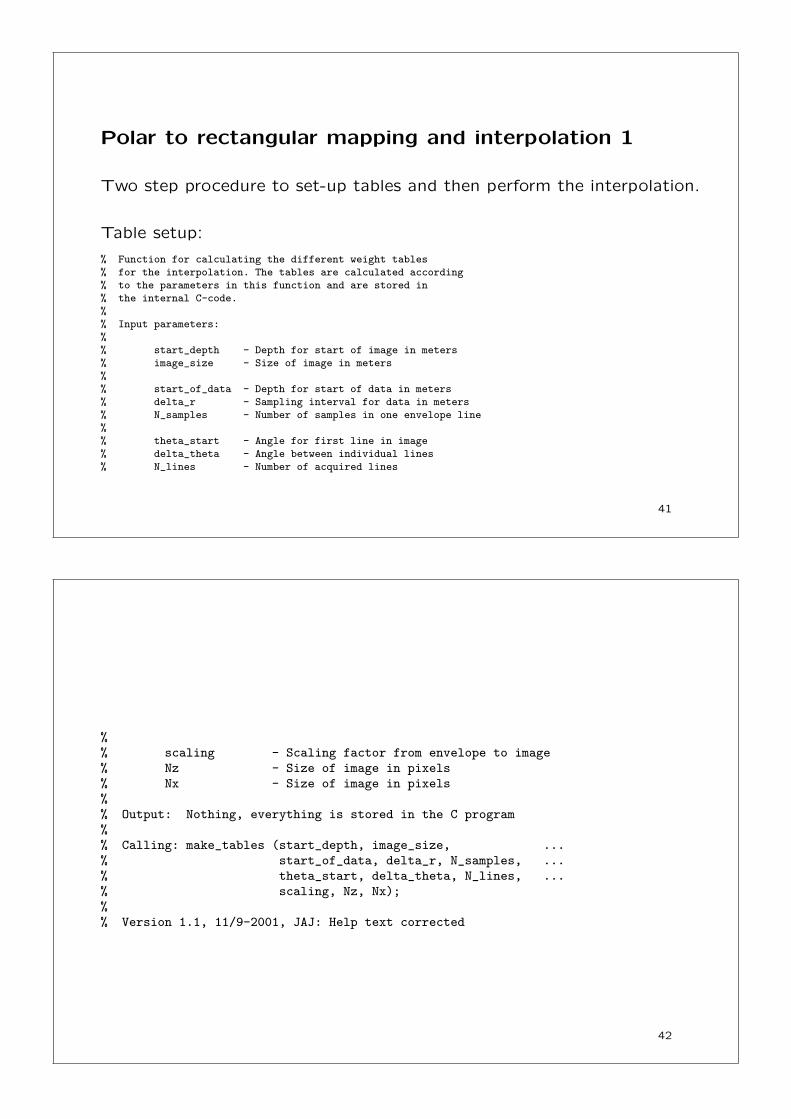
Signal processing in ultrasound system - Exercise 1

Transmit/receive

Beamsteering

Time-gaincompensation

Detector

Memory

Control

Imagearea

Sweepingbeam

Display

Scanconverter

Signal processing in a simple ultrasound system with a single element

ultrasound transducer.

39

Signal processing

1. Acquire RF data (load from file)

2. Perform Hilbert transform to find envelope:env(n) = |y(n)2 +H{y(n)}2|

3. Compress the dynamic range to 50 dB:log env(n) = 20 log10(env(n))

4. Scale to the color map range (128 gray levels)

5. Make polar to rectangular mapping and interpolation

6. Display the image

7. Load a number of clinical images and make a movie

40

Polar to rectangular mapping and interpolation 1

Two step procedure to set-up tables and then perform the interpolation.

Table setup:

% Function for calculating the different weight tables% for the interpolation. The tables are calculated according% to the parameters in this function and are stored in% the internal C-code.%% Input parameters:%% start_depth - Depth for start of image in meters% image_size - Size of image in meters%% start_of_data - Depth for start of data in meters% delta_r - Sampling interval for data in meters% N_samples - Number of samples in one envelope line%% theta_start - Angle for first line in image% delta_theta - Angle between individual lines% N_lines - Number of acquired lines

41

%% scaling - Scaling factor from envelope to image% Nz - Size of image in pixels% Nx - Size of image in pixels%% Output: Nothing, everything is stored in the C program%% Calling: make_tables (start_depth, image_size, ...% start_of_data, delta_r, N_samples, ...% theta_start, delta_theta, N_lines, ...% scaling, Nz, Nx);%% Version 1.1, 11/9-2001, JAJ: Help text corrected

42

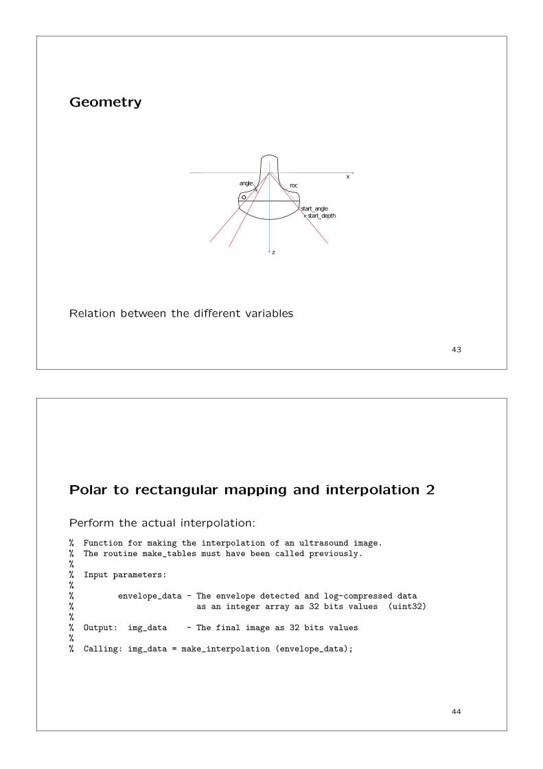
Geometry

x

z

angle

start_anglestart_depth

roc

Relation between the different variables

43

Polar to rectangular mapping and interpolation 2

Perform the actual interpolation:

% Function for making the interpolation of an ultrasound image.% The routine make_tables must have been called previously.%% Input parameters:%% envelope_data - The envelope detected and log-compressed data% as an integer array as 32 bits values (uint32)%% Output: img_data - The final image as 32 bits values%% Calling: img_data = make_interpolation (envelope_data);

44

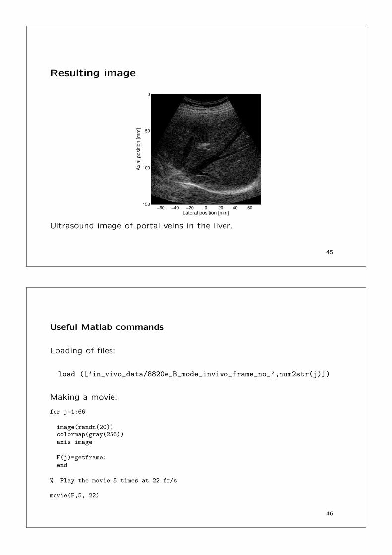
Resulting image

Lateral position [mm]

Axia

l p

ositio

n [

mm

]

−60 −40 −20 0 20 40 60

0

50

100

150

Ultrasound image of portal veins in the liver.

45

Useful Matlab commands

Loading of files:

load ([’in_vivo_data/8820e_B_mode_invivo_frame_no_’,num2str(j)])

Making a movie:

for j=1:66

image(randn(20))colormap(gray(256))axis image

F(j)=getframe;end

% Play the movie 5 times at 22 fr/s

movie(F,5, 22)

46

Discussion for next time

Use the ultrasound system from the first discussion assignment

1. What is the largest pressure tolerated for cardiac imaging?

2. What displacement will this give rise to in tissue?

Prepare your Matlab code for exercise 1.

47