3.1 THREE DIMENSIONAL CONCEPTS - SJCET, PALAImcasjcet.weebly.com/uploads/4/4/7/9/4479347/computer_graphics... · by a set of surface polygons. Many graphic ... representations are

MODULE II I MCA - 301 COMPUTER GRAPHICS ADMN 2009-‘10

Dept. of Computer Science And Applications, SJCET, Palai 75

3.1 THREE DIMENSIONAL CONCEPTS

We can rotate an object about an axis with any spatial orientation in three-

dimensional space. Two-dimensional rotations, on the other hand, are always around an

axis that is perpendicular to the xy plane. Viewing transformations in three dimensions

are much more cornplicated because we have many more parameters to select when

specifying how a three-dimensional scene is to be mapped to a display device. The scene

description must be processed through viewing-coordinate transformations and

projection routines that transform three-dimensional viewing coordinates onto two-

dimensional device coordinates. Visible parts of a scene, for a selected view, must be

identified; and surface-rendering algorithms must he applied if a realistic rendering of

the scene is required.

3.2 THREE DIMENSIONAL OBJECT REPRESENTATIONS

Graphics scenes contain many different kinds of objects. Trees, flowers, glass,

rock, water etc.. There is not any single method that we can use to describe objects that

will include all characteristics of these different materials.

Polygon and quadric surfaces provide precise descriptions for simple Euclidean

objects such as polyhedrons and ellipsoids.

Spline surfaces and construction techniques are useful for designing aircraft

wings, gears and other engineering structure with curved surfaces.

Procedural methods such as fractal constructions and particle systems allow us to

give accurate representations for clouds, clumps of grass and other natural objects.

Physically based modeling methods using systems of interacting forces can be

used to describe the non-rigid behavior of a piece of cloth or a glob of jello.

Octree encodings are used to represent internal features of objects; such as those

obtained from medical CT images.

Isosurface displays, volume renderings and other visualization techniques are

applied to 3 dimensional discrete data sets to obtain visual representations of the data.

3.3 POLYGON SURFACES

Polygon surfaces provide precise descriptions for simple Euclidean objects such

as polyhedrons and ellipsoids. A three dimensional graphics object can be represented

by a set of surface polygons. Many graphic systems store a 3 dimensional object as a set

of surface polygons. This simplifies and speeds up the surface rendering and display of

objects. In this representation, the surfaces are described with linear equations. The

polygonal representation of a polyhedron precisely defines the surface features of an

object.

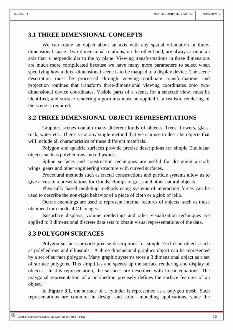
In Figure 3.1, the surface of a cylinder is represented as a polygon mesh. Such

representations are common in design and solid- modeling applications, since the



wireframe outline can be displayed quickly to give a general indication of the surface

structure.

(Figure 3.1, Wireframe representation of a cylinder with back (hidden) lines removed)

3.4 POLYGON TABLES

We know that a polygon surface is defined by a set of vertices. As information

for each polygon is input, the data are placed in to tables that are used in later

processing, display and manipulation of objects in the scene.

Polygon data tables can be organized in to 2 groups: geometric tables and

attribute tables. Geometric data tables contain vertex coordinates and parameters to

identify the spatial orientation of the polygon surfaces. Attribute information for an

object includes parameters specifying the degree of transparency of the object and its

surface reflexivity and texture characteristics.

A suitable organization for storing geometric data is to create 3 lists, a vertex

table, an edge table and a polygon table. Coordinate values for each vertex is stored in

the vertex table. The edge table contains pointers back to the vertex table to identify the

vertices for each polygon edge. The polygon table contains pointers back to the edge

table to identify the edges for each polygon.

An alternative arrangement is to modify the edge table to include forward

pointers in to the polygon table so that common edges between polygons could be

identified more rapidly.

Additional geometric formation that is usually stored in the data tables includes

the slope for each edge and the coordinate extents for each polygon. As vertices are

input, we can calculate edge slopes, and we can scan the coordinate values to identify

the minimum and maximum x, y, and z values for individual polygons. Edge slopes and

bounding-box information for the polygons are needed in subsequent processing, for

example, surface rendering. Coordinate extents are also used in some visible-surface

determination algorithms

The more information included in the data tables, the easier it is to check for

errors. Therefore, error checking is easier when three data tables (vertex, edge, and

polygon) are used, since this scheme provides the most information. Some of the tests



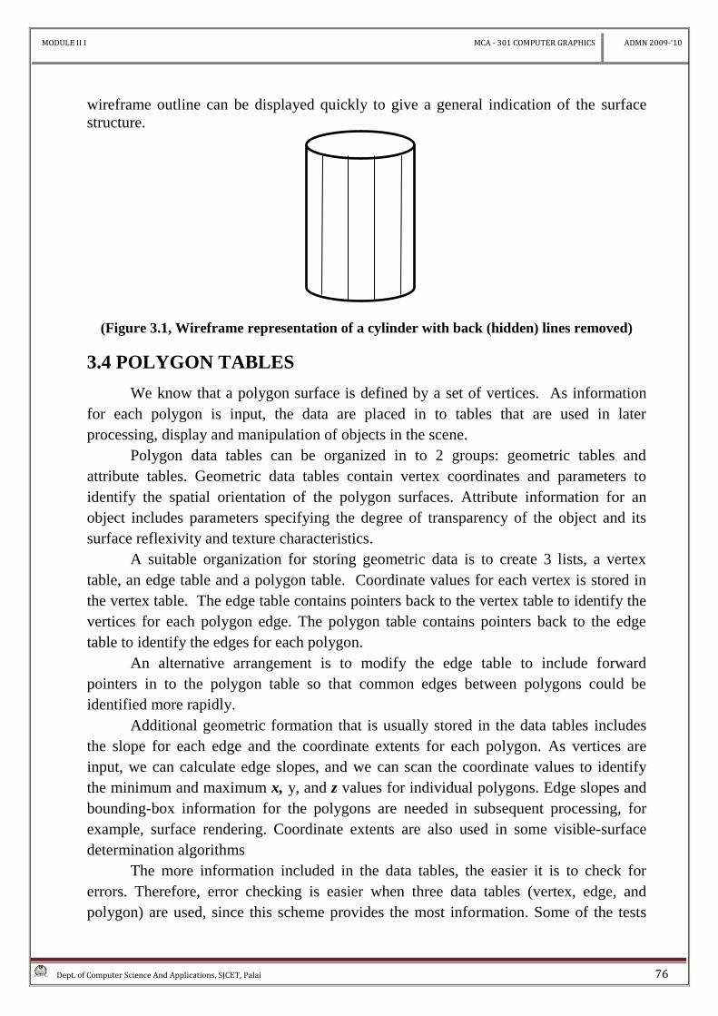
that could be performed by a graphics package are (1) that every vertex is listed as an

endpoint for at least two edges, (2) that every edge is part of at least one polygon, (3)

that every polygon is closed, (4) that each polygon has at least one shared edge, and (5)

that if the edge table contains pointers to polygons, every edge referenced by a polygon

pointer has a reciprocal pointer back to the polygon.

3.5 PLANE EQUATIONS When working with polygons or polygon meshes, we need to know the equation

of the plane in which the polygon lies. We can use the coordinates of 3 vertices to find

the plane. The plane equation is

Ax + By + Cz + D = 0

The coefficients A, B and C define the normal to the plane. [A B C]. We can

obtain the coefficients A, B, C and D by solving a set of 3 plane equations using the

coordinate values for 3 non collinear points in the plane. Suppose we have 3 vertices on

the polygon (x1, y1, z1), (x2, y2, z2) and (x3, y3, z3).

Ax + By + Cz + D = 0

(A/D) x1 + (B/D) y1 + (C/D) z1 = -1

(A/D) x2 + (B/D) y2 + (C/D) z2 = -1

(A/D) x3 + (B/D) y3 + (C/D) z3 = -1

the solution for this set of equations can be obtained using Cramer‘s rule as,

VERTEX

TABLE

V1:x1,y1,z1

V2:x2,y2,z2

V3:x3,y3,z3

V4:x4,y4,z4

V5:x5,y5,z5

EDGE TABLE

E1:V1,V2

E2:V2,V3

E3:V3,V1

E4:V3,V4

E5:V4,V5

E6:V5,V1

POLYGON-SURFACE

TABLE

S1:E1,E2,E3

S2:E3,E4,E5,E6



A = 1 y1 z1

1 y2 z2

1 y3 z3

B = x1 1 z1

x2 1 z2

x3 1 z3

C = x1 y1 1

x2 y2 1

x3 y3 1

D = _ x1 y1 z1

x2 y2 z2

x3 y3 z3

We can write the calculations for the plane coefficients in the form

A = y1 (z2 - z3) + y2 (z3 – z1) + y3 (z1 – z2)

B = z1 (x2 - x3) + z2 (x3 – x1) + z3 (x1 – x2)

C = x1 (y2 - y3) + x2 (y3 – y1) + x3 (y1 – y2)

D= - x1 (y2 z3 – y3 z2) – x2 (y3 z1 – y1 z3) – x3 (y1 z2 – y2 z1)

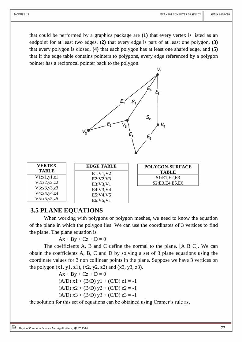
(Figure 3.2, The vector N, Normal to the surface of a plane described by the equation

Ax + By + Cz + D = 0 ,has Cartesian components(A,B,C))

If there are more than 3 vertices, the polygon may be non-planar. We can check

whether a polygon is nonplanar by calculating the perpendicular distance from the plane

to each vertex. The distance d for the vertex at (x, y, z) is

d = Ax + By + Cz + D

(A2 + B

2 + C

2)

N=(A,B,C)



The distance is either positive or negative, depending on which side of the plane the

point is located. If the vertex is on the plane, then d = 0.

We can identify the point as either inside or outside the plane surface according to

the sign of Ax + By + Cz + D.

If Ax + By + Cz + D < 0, the point (x, y, z) is inside the surface.

If Ax + By + Cz + D > 0, the point (x, y, z) is outside the surface.

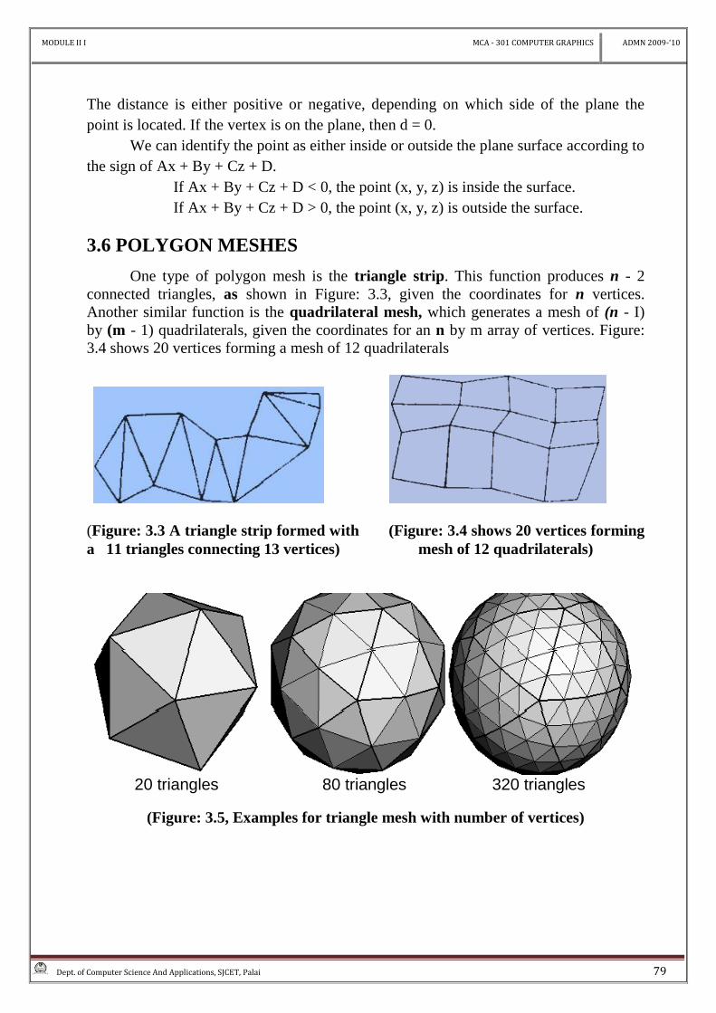
3.6 POLYGON MESHES

One type of polygon mesh is the triangle strip. This function produces n - 2

connected triangles, as shown in Figure: 3.3, given the coordinates for n vertices.

Another similar function is the quadrilateral mesh, which generates a mesh of (n - I)

by (m - 1) quadrilaterals, given the coordinates for an n by m array of vertices. Figure:

3.4 shows 20 vertices forming a mesh of 12 quadrilaterals

(Figure: 3.3 A triangle strip formed with (Figure: 3.4 shows 20 vertices forming

a 11 triangles connecting 13 vertices) mesh of 12 quadrilaterals)

20 triangles 80 triangles 320 triangles

(Figure: 3.5, Examples for triangle mesh with number of vertices)



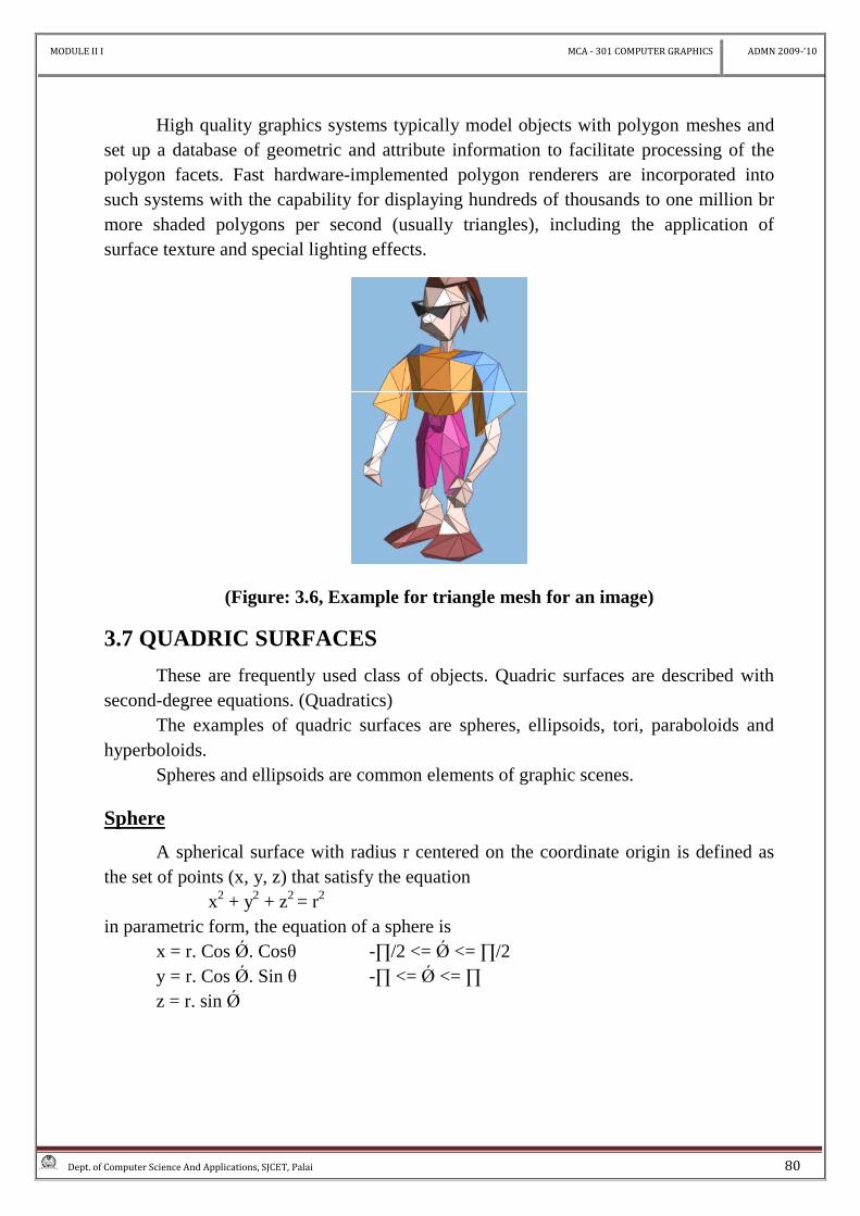
High quality graphics systems typically model objects with polygon meshes and

set up a database of geometric and attribute information to facilitate processing of the

polygon facets. Fast hardware-implemented polygon renderers are incorporated into

such systems with the capability for displaying hundreds of thousands to one million br

more shaded polygons per second (usually triangles), including the application of

surface texture and special lighting effects.

(Figure: 3.6, Example for triangle mesh for an image)

3.7 QUADRIC SURFACES

These are frequently used class of objects. Quadric surfaces are described with

second-degree equations. (Quadratics)

The examples of quadric surfaces are spheres, ellipsoids, tori, paraboloids and

hyperboloids.

Spheres and ellipsoids are common elements of graphic scenes.

Sphere

A spherical surface with radius r centered on the coordinate origin is defined as

the set of points (x, y, z) that satisfy the equation

x2 + y

2 + z

2 = r

2

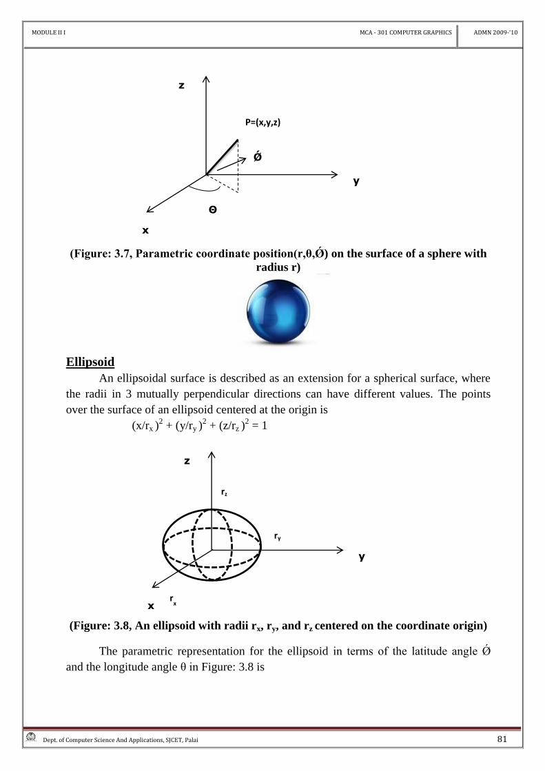
in parametric form, the equation of a sphere is

x = r. Cos Ǿ. Cosθ -∏/2 <= Ǿ <= ∏/2

y = r. Cos Ǿ. Sin θ -∏ <= Ǿ <= ∏

z = r. sin Ǿ



(Figure: 3.7, Parametric coordinate position(r,θ,Ǿ) on the surface of a sphere with

radius r)

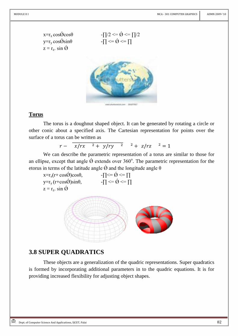
Ellipsoid

An ellipsoidal surface is described as an extension for a spherical surface, where

the radii in 3 mutually perpendicular directions can have different values. The points

over the surface of an ellipsoid centered at the origin is

(x/rx )2 + (y/ry )

2 + (z/rz )

2 = 1

(Figure: 3.8, An ellipsoid with radii rx, ry, and rz centered on the coordinate origin)

The parametric representation for the ellipsoid in terms of the latitude angle Ǿ

and the longitude angle θ in Figure: 3.8 is

P=(x,y,z)

x

z

y

Ǿ

rz

x

z

y

ry

rx



x=rx cosǾcosθ -∏/2 <= Ǿ <= ∏/2

y=ry cosǾsinθ -∏ <= Ǿ <= ∏

z = rz. sin Ǿ

Torus

The torus is a doughnut shaped object. It can be generated by rotating a circle or

other conic about a specified axis. The Cartesian representation for points over the

surface of a torus can be written as

We can describe the parametric representation of a torus are similar to those for

an ellipse, except that angle Ǿ extends over 360o. The parametric representation for the

etorus in terms of the latitude angle Ǿ and the longitude angle θ

x=rx(r+ cosǾ)cosθ, -∏<= Ǿ <= ∏

y=ry (r+cosǾ)sinθ, -∏ <= Ǿ <= ∏

z = rz. sin Ǿ

3.8 SUPER QUADRATICS

These objects are a generalization of the quadric representations. Super quadratics

is formed by incorporating additional parameters in to the quadric equations. It is for

providing increased flexibility for adjusting object shapes.



Super ellipse

The Cartesian representation for a super ellipse is obtained from the equation of

an ellipse by allowing the exponent on the x and y terms to be variable.

The equation of a super ellipse is

+

The parameter s can be assigned any real value. When s = 1, we get an ordinary

ellipse. Corresponding parametric equations for the superellipse can be expressed as

x=rxcossθ, -∏<= Ǿ <= ∏

y=rysinsθ,

.,;, ·. ,;

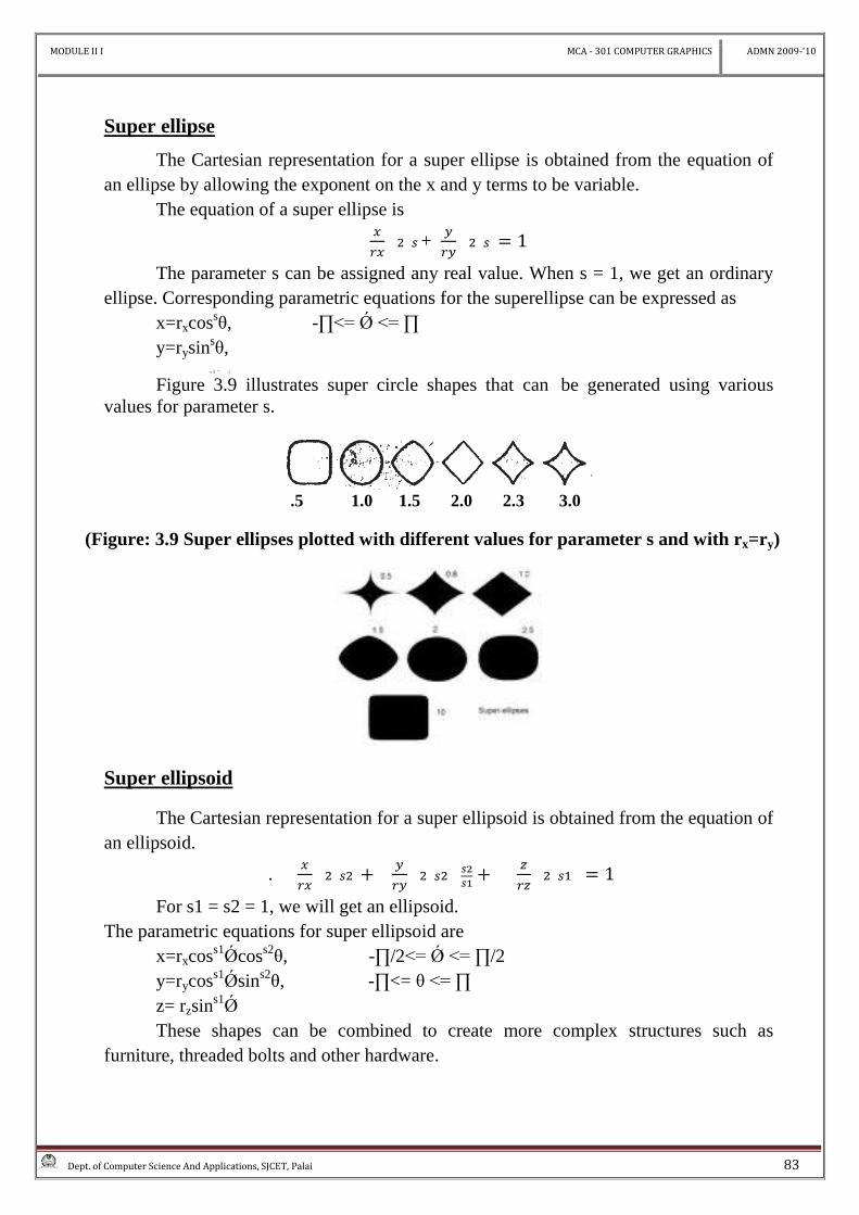
Figure 3.9 illustrates super circle shapes that can be generated using various

values for parameter s.

.5 1.0 1.5 2.0 2.3 3.0

(Figure: 3.9 Super ellipses plotted with different values for parameter s and with rx=ry)

Super ellipsoid

The Cartesian representation for a super ellipsoid is obtained from the equation of

an ellipsoid.

.

For s1 = s2 = 1, we will get an ellipsoid.

The parametric equations for super ellipsoid are

x=rxcoss1

Ǿcoss2

θ, -∏/2<= Ǿ <= ∏/2

y=rycoss1

Ǿsins2

θ, -∏<= θ <= ∏

z= rzsins1

Ǿ

These shapes can be combined to create more complex structures such as

furniture, threaded bolts and other hardware.



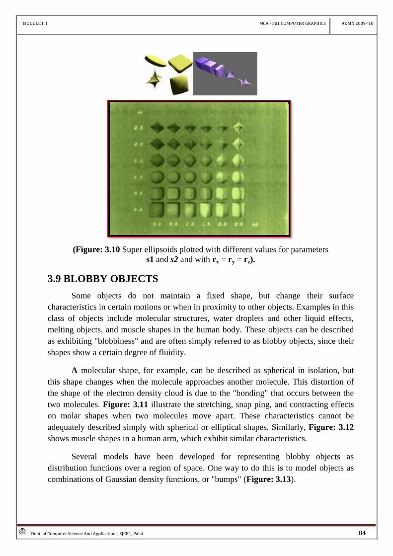
(Figure: 3.10 Super ellipsoids plotted with different values for parameters

s1 and s2 and with rx = ry = rz).

3.9 BLOBBY OBJECTS

Some objects do not maintain a fixed shape, but change their surface

characteristics in certain motions or when in proximity to other objects. Examples in this

class of objects include molecular structures, water droplets and other liquid effects,

melting objects, and muscle shapes in the human body. These objects can be described

as exhibiting "blobbiness" and are often simply referred to as blobby objects, since their

shapes show a certain degree of fluidity.

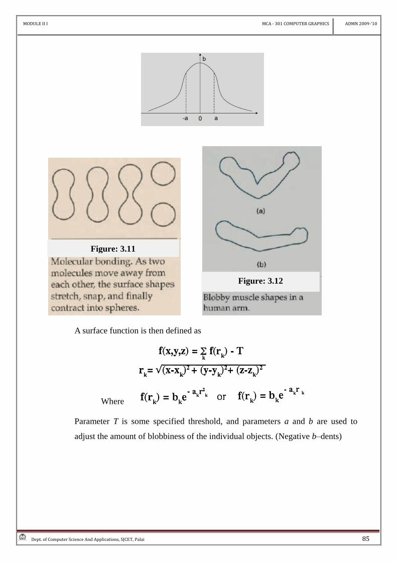
A molecular shape, for example, can be described as spherical in isolation, but

this shape changes when the molecule approaches another molecule. This distortion of

the shape of the electron density cloud is due to the "bonding" that occurs between the

two molecules. Figure: 3.11 illustrate the stretching, snap ping, and contracting effects

on molar shapes when two molecules move apart. These characteristics cannot be

adequately described simply with spherical or elliptical shapes. Similarly, Figure: 3.12

shows muscle shapes in a human arm, which exhibit similar characteristics.

Several models have been developed for representing blobby objects as

distribution functions over a region of space. One way to do this is to model objects as

combinations of Gaussian density functions, or "bumps" (Figure: 3.13).



A surface function is then defined as

Where

Parameter T is some specified threshold, and parameters a and b are used to

adjust the amount of blobbiness of the individual objects. (Negative b–dents)

Figure: 3.11

Figure: 3.12



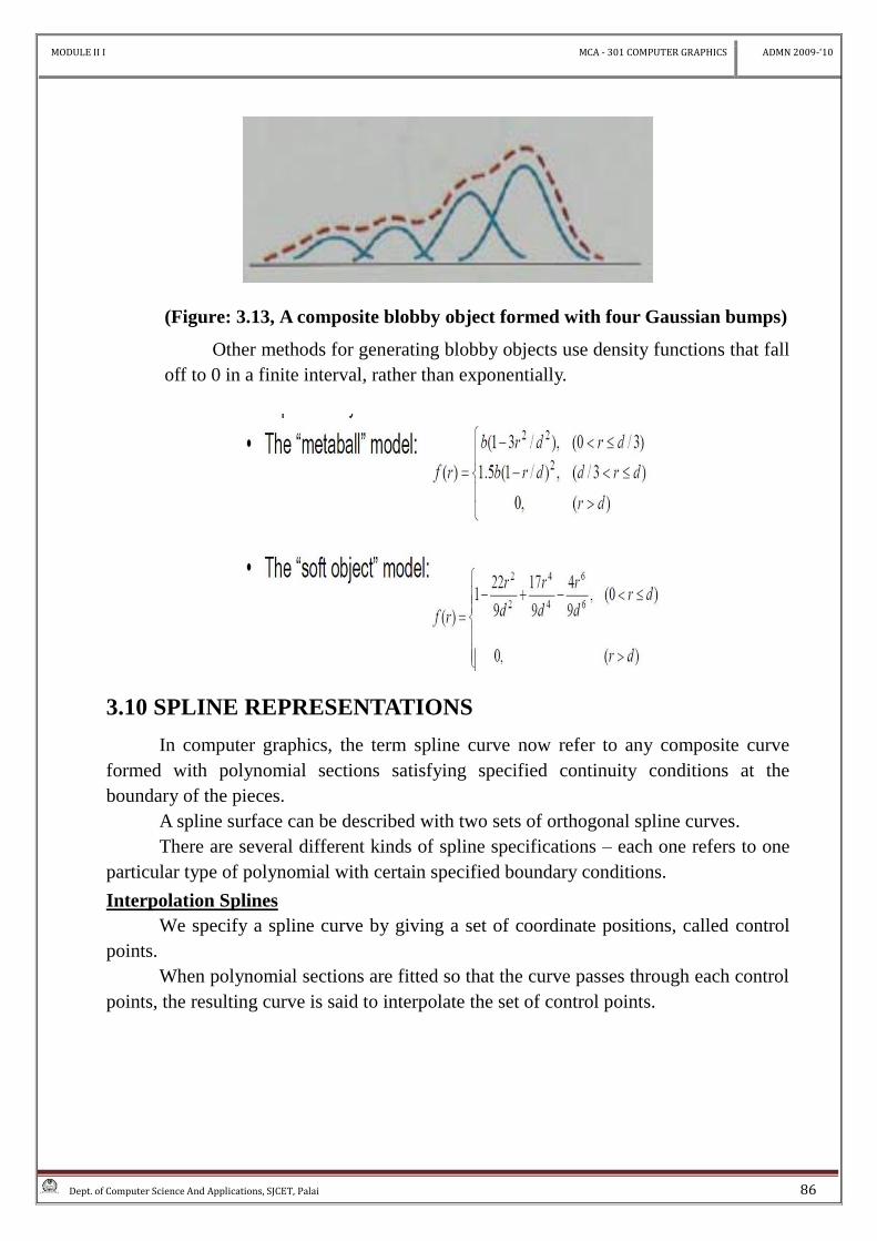
(Figure: 3.13, A composite blobby object formed with four Gaussian bumps)

Other methods for generating blobby objects use density functions that fall

off to 0 in a finite interval, rather than exponentially.

3.10 SPLINE REPRESENTATIONS

In computer graphics, the term spline curve now refer to any composite curve

formed with polynomial sections satisfying specified continuity conditions at the

boundary of the pieces.

A spline surface can be described with two sets of orthogonal spline curves.

There are several different kinds of spline specifications – each one refers to one

particular type of polynomial with certain specified boundary conditions.

Interpolation Splines

We specify a spline curve by giving a set of coordinate positions, called control

points.

When polynomial sections are fitted so that the curve passes through each control

points, the resulting curve is said to interpolate the set of control points.



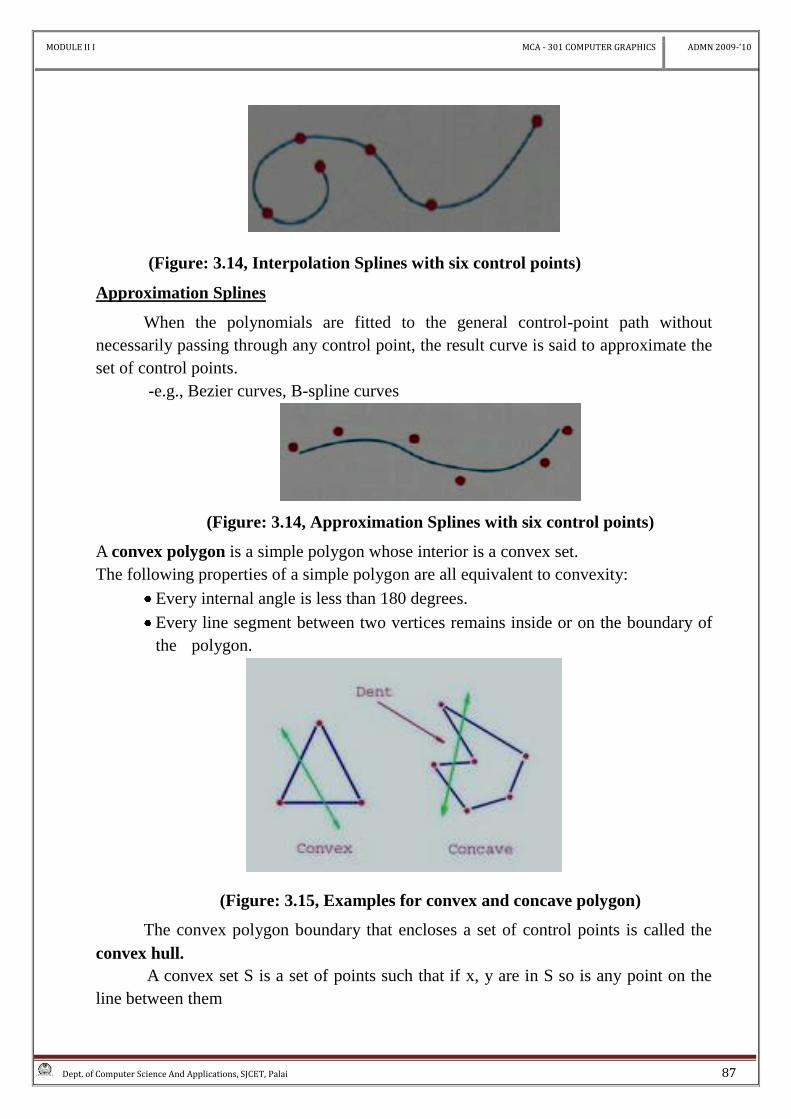
(Figure: 3.14, Interpolation Splines with six control points)

Approximation Splines

When the polynomials are fitted to the general control-point path without

necessarily passing through any control point, the result curve is said to approximate the

set of control points.

-e.g., Bezier curves, B-spline curves

(Figure: 3.14, Approximation Splines with six control points)

A convex polygon is a simple polygon whose interior is a convex set.

The following properties of a simple polygon are all equivalent to convexity:

Every internal angle is less than 180 degrees.

Every line segment between two vertices remains inside or on the boundary of

the polygon.

(Figure: 3.15, Examples for convex and concave polygon)

The convex polygon boundary that encloses a set of control points is called the

convex hull.

A convex set S is a set of points such that if x, y are in S so is any point on the

line between them

http://en.wikipedia.org/wiki/Simple_polygon

http://en.wikipedia.org/wiki/Interior_(topology)

http://en.wikipedia.org/wiki/Convex_set

http://en.wikipedia.org/wiki/Internal_angle

http://en.wikipedia.org/wiki/Degree_(angle)

http://en.wikipedia.org/wiki/Line_segment

http://en.wikipedia.org/wiki/Vertex_(geometry)



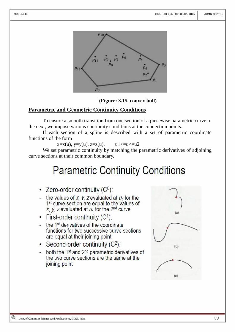
(Figure: 3.15, convex hull)

Parametric and Geometric Continuity Conditions

To ensure a smooth transition from one section of a piecewise parametric curve to

the next, we impose various continuity conditions at the connection points.

If each section of a spline is described with a set of parametric coordinate

functions of the form

x=x(u), y=y(u), z=z(u), u1<=u<=u2

We set parametric continuity by matching the parametric derivatives of adjoining

curve sections at their common boundary.



3.10.1 BEZIER CURVES AND SURFACES

Bezier splines have a number of properties that make them highly useful and

convenient for curve and surface design.

They are also easy to implement.

Bezier splines are widely available in various CAD systems.

The number of control points to be approximated and their relative position determine

the degree of the Bezier polynomial.

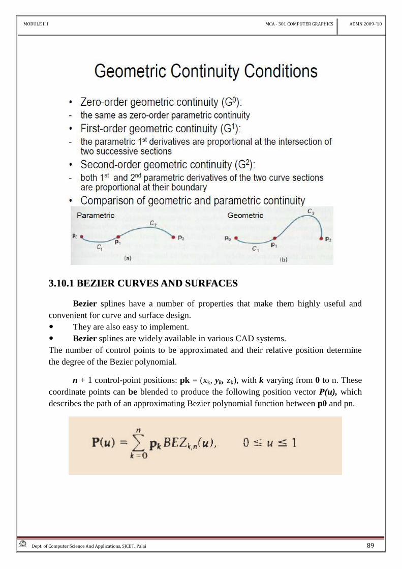
n + 1 control-point positions: pk = (xk, yk, zk), with k varying from 0 to n. These

coordinate points can be blended to produce the following position vector P(u), which

describes the path of an approximating Bezier polynomial function between p0 and pn.



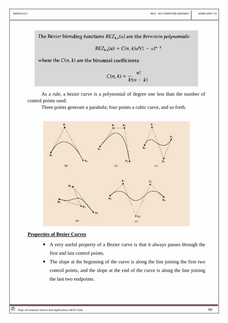
As a rule, a bezier curve is a polynomial of degree one less than the number of

control points used:

Three points generate a parabola; four points a cubic curve, and so forth.

Properties of Bezier Curves

A very useful property of a Bezier curve is that it always passes through the

first and last control points.

The slope at the beginning of the curve is along the line joining the first two

control points, and the slope at the end of the curve is along the line joining

the last two endpoints.



Another important property of any Bezier curve is that it lies within the

convex hull (convex polygon boundary) of the control points.

Design Techniques using Bezier curve

Closed Bezier curves are generated by specifying the first and last control

points at the same position.

Also, specifying multiple control points at a single coordinate position gives

more weight to that position.

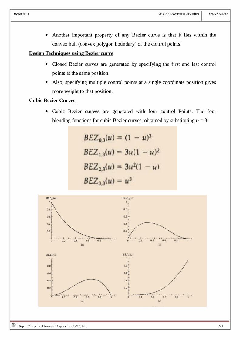
Cubic Bezier Curves

Cubic Bezier curves are generated with four control Points. The four

blending functions for cubic Bezier curves, obtained by substituting n = 3



At u = 0, the only nonzero blending function is BEZ0, 3, which has the

value 1.

At u = 1, the only nonzero function is BEZ3, 3 with a value of 1 at that

point.

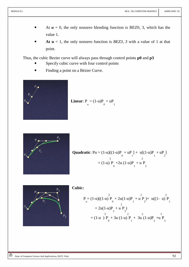
Thus, the cubic Bezier curve will always pass through control points p0 and p3

Specify cubic curve with four control points

Finding a point on a Bézier Curve.

Linear: Pu = (1-u)P

0 + uP

1

Quadratic: Pu = (1-u)[(1-u)P0 + uP

1] + u[(1-u)P

1 + uP

2]

= (1-u)2

P0 +2u (1-u)P

1 + u

2

P2

Cubic:

Pu= (1-u)((1-u)

2

P0 + 2u(1-u)P

1 + u

2

P2)+ u((1- u)

2

P1

+ 2u(1-u)P2 + u

2

P3)

= (1-u )3

P0 + 3u (1-u)

2

P1 + 3u

2

(1-u)P2 +u

3

P3



BÉZIER SURFACE

A Bézier surface S(u,v) is defined by a grid of control points Pi,j

, where

0 i m, 0 j n, and 0 u 1, 0 v 1. The degree is (m,n).

Bm,i

(u) Bn,j

(v) are the Bézier basis functions for the surface.

This Bezier surface has a degree of (4,3).

Important Properties

S(u,v) passes through the control points at the four corners of the control net:

P0,0

, Pm,0

, Pm,n

, P0,n

.

Partition of unity:

Convex hull property: a Bézier surface lies in the convex hull defined by its

control net.

i j

jijnim PvBuBvuS ,,, )()(),(

jnj

jn

imi

im

vvjnj

nvB

uuimi

muB

)1()!(!

!)(

)1()!(!

!)(

,

,

m

i

n

j

jnim vBuB0 0

,, 1)()(

Documents

3.1 THREE DIMENSIONAL CONCEPTS - SJCET, PALAImcasjcet.weebly.com/uploads/4/4/7/9/4479347/computer_graphics... · by a set of surface polygons. Many graphic ... representations are