3017 Tutorial 4 Solutions

7/16/2019 3017 Tutorial 4 Solutions

http://slidepdf.com/reader/full/3017-tutorial-4-solutions 1/3

FINC3017 Investments and Portfolio Management

Tutorial 4 Solutions

Single Index Model

1. Estimate the Single-Index Model for Cabcharge, David Jones, Macquarie

Group and Tabcorp using excess returns for the full sample from 31 January

2001 to 31 July 2012.

a) Which stock has greater systematic risk? Comment on the differences in

the estimates of systematic risk across the four companies.

b) Which stock has the highest firm-specific risk?

c) Which stock has the highest alpha?

d) Which stock would you want to invest in for the next 12 months?

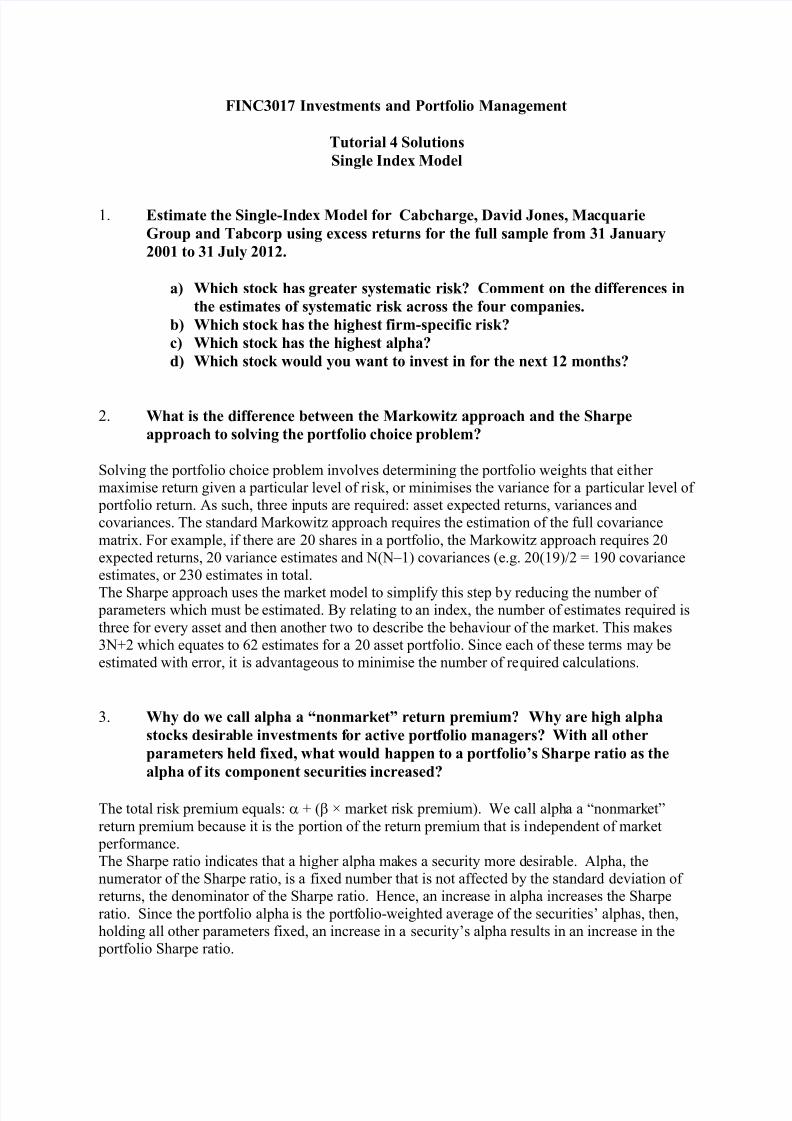
2. What is the difference between the Markowitz approach and the Sharpe

approach to solving the portfolio choice problem?

Solving the portfolio choice problem involves determining the portfolio weights that either

maximise return given a particular level of risk, or minimises the variance for a particular level of

portfolio return. As such, three inputs are required: asset expected returns, variances and

covariances. The standard Markowitz approach requires the estimation of the full covariance

matrix. For example, if there are 20 shares in a portfolio, the Markowitz approach requires 20

expected returns, 20 variance estimates and N(N – 1) covariances (e.g. 20(19)/2 = 190 covariance

estimates, or 230 estimates in total.

The Sharpe approach uses the market model to simplify this step by reducing the number of parameters which must be estimated. By relating to an index, the number of estimates required is

three for every asset and then another two to describe the behaviour of the market. This makes

3N+2 which equates to 62 estimates for a 20 asset portfolio. Since each of these terms may be

estimated with error, it is advantageous to minimise the number of required calculations.

3. Why do we call alpha a “nonmarket” return premium? Why are high alpha

stocks desirable investments for active portfolio managers? With all other

parameters held fixed, what would happen to a portfolio’s Sharpe ratio as the

alpha of its component securities increased?

The total risk premium equals: + ( × market risk premium). We call alpha a “nonmarket”

return premium because it is the portion of the return premium that is independent of market

performance.

The Sharpe ratio indicates that a higher alpha makes a security more desirable. Alpha, the

numerator of the Sharpe ratio, is a fixed number that is not affected by the standard deviation of

returns, the denominator of the Sharpe ratio. Hence, an increase in alpha increases the Sharpe

ratio. Since the portfolio alpha is the portfolio-weighted average of the securities’ alphas, then,

holding all other parameters fixed, an increase in a security’s alpha results in an increase in the

portfolio Sharpe ratio.



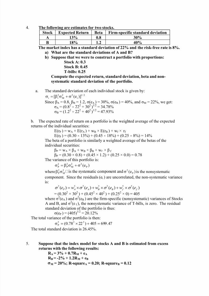
4. The following are estimates for two stocks.

Stock Expected Return Beta Firm-specific standard deviation

A 13% 0.8 30%

B 18% 1.2 40%

The market index has a standard deviation of 22% and the risk-free rate is 8%.

a) What are the standard deviations of A and B?b) Suppose that we were to construct a portfolio with proportions:

Stock A: 0.3

Stock B: 0.45

T-bills: 0.25

Compute the expected return, standard deviation, beta and non-

systematic standard deviation of the portfolio.

a. The standard deviation of each individual stock is given by:2/1

i

22

M

2

ii )]e([

Since βA = 0.8, βB = 1.2, σ(eA ) = 30%, σ(eB ) = 40%, and σM = 22%, we get:σA = (0.82 × 222 + 302 )1/2 = 34.78%

σB = (1.22 × 222 + 402 )1/2 = 47.93%

b. The expected rate of return on a portfolio is the weighted average of the expected

returns of the individual securities:

E(r P ) = wA × E(r A ) + wB × E(r B ) + wf × r f

E(r P ) = (0.30 × 13%) + (0.45 × 18%) + (0.25 × 8%) = 14%

The beta of a portfolio is similarly a weighted average of the betas of the

individual securities:

βP = wA × βA + wB × βB + wf × β f

βP = (0.30 × 0.8) + (0.45 × 1.2) + (0.25 × 0.0) = 0.78The variance of this portfolio is:

)e( P

22

M

2

P

2

P

where2

M

2

P )e( P

2 is the nonsystematic

component. Since the residuals (ei ) are uncorrelated, the non-systematic variance

is:2 2 2 2 2 2 2( ) ( ) ( ) ( ) P A A B B f f e w e w e w e

= (0.302 × 302 ) + (0.452 × 402 ) + (0.252 × 0) = 405

where σ2(eA ) and σ2(eB ) are the firm-specific (nonsystematic) variances of Stocks

A and B, and σ2(e f ), the nonsystematic variance of T-bills, is zero. The residual

standard deviation of the portfolio is thus:σ(eP ) = (405)1/2 = 20.12%

The total variance of the portfolio is then:

47.699405)2278.0(222

P

The total standard deviation is 26.45%.

5. Suppose that the index model for stocks A and B is estimated from excess

returns with the following results:

R A = 3% + 0.7R M + eA

R B = -2% + 1.2R M + eB

M = 20%; R-squareA = 0.20; R-squareB = 0.12



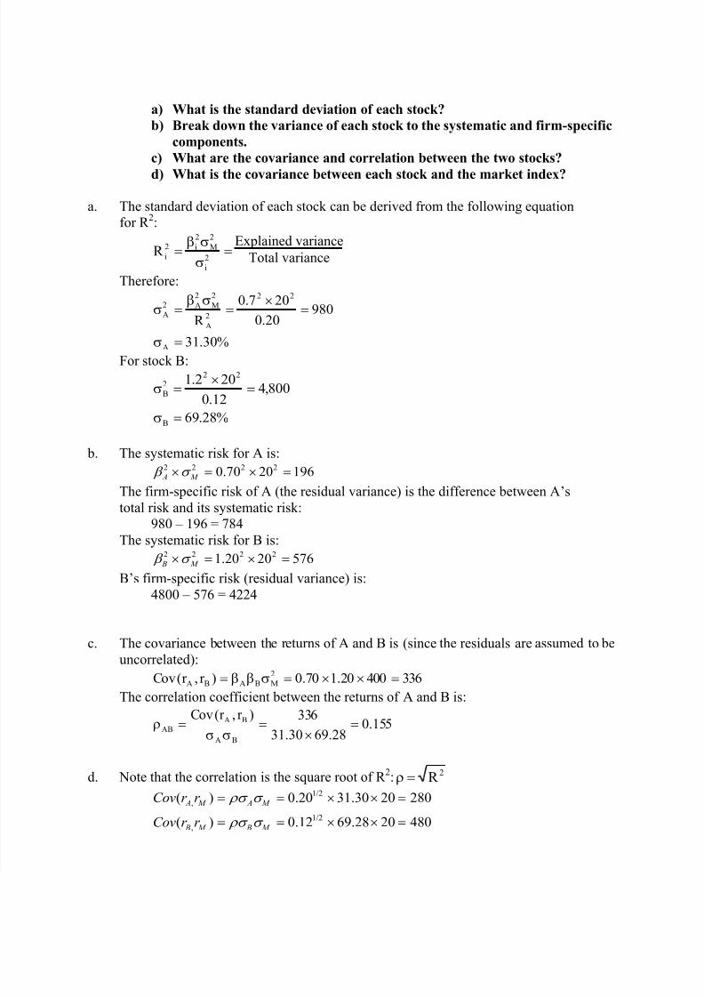
a) What is the standard deviation of each stock?

b) Break down the variance of each stock to the systematic and firm-specific

components.

c) What are the covariance and correlation between the two stocks?

d) What is the covariance between each stock and the market index?

a. The standard deviation of each stock can be derived from the following equation

for R 2:

2

i

2

M

2

i2

iR Explained variance

Total variance

Therefore:

%30.31

98020.0

207.0

R

A

22

2

A

2

M

2

A2

A

For stock B:

%28.69

800,412.0

202.1

B

222

B

b. The systematic risk for A is:2 2 2 20.70 20 196 A M

The firm-specific risk of A (the residual variance) is the difference between A’s

total risk and its systematic risk:

980 – 196 = 784The systematic risk for B is:

2 2 2 21.20 20 576 B M

B’s firm-specific risk (residual variance) is:

4800 – 576 = 4224

c. The covariance between the returns of A and B is (since the residuals are assumed to be

uncorrelated):

33640020.170.0)r ,r (Cov2

MBABA

The correlation coefficient between the returns of A and B is:

155.028.6930.31

336)r ,r (Cov

BA

BA

AB

d. Note that the correlation is the square root of R 2: 2R 1/2

,

1/2

,

( ) 0.20 31.30 20 280

( ) 0.12 69.28 20 480

A M A M

B M B M

Cov r r

Cov r r

Documents

3017 Tutorial 4 Solutions