30 November 2006. math.AG/0602161sottile/research/pdf/quot.pdf30 November 2006. math.AG/0602161 THE EQUIVARIANT CHOW RINGS OF QUOT SCHEMES TOM BRADEN, LINDA CHEN, AND FRANK SOTTILE

30 November 2006. math.AG/0602161

THE EQUIVARIANT CHOW RINGS OF QUOT SCHEMES

TOM BRADEN, LINDA CHEN, AND FRANK SOTTILE

Abstract. We give a presentation for the (integral) torus-equivariant Chow ring ofthe quot scheme, a smooth compactification of the space of rational curves of degree d inthe Grassmannian. For this presentation, we refine Evain’s extension of the method ofGoresky, Kottwitz, and MacPherson to express the torus-equivariant Chow ring in termsof the torus-fixed points and explicit relations coming from the geometry of families oftorus-invariant curves. As part of this calculation, we give a complete description ofthe torus-invariant curves on the quot scheme and show that each family is a productof projective spaces.

Introduction

Let k be an algebraically closed field and let d, n, r be non-negative integers withr < n. We study the quot scheme Qd := Qd(r, n) parametrizing quotient sheaves on P1

of the trivial vector bundle OnP1 which have rank r and degree d. When r > 0, this is

a compactification of the space Md of parametrized rational curves of degree d on theGrassmannian G(r, n) of r-dimensional quotients of kn. Indeed, a morphism from P1 toG(r, n) of degree d is equivalent to a quotient bundle On

P1 → T of rank r and degree d.Strømme [16] showed that Qd(r, n) is a smooth, projective, rational variety of dimen-

sion r(n− r) + nd. He described the decomposition into BiaÃlynicki-Birula cells inducedby an action of a one-dimensional torus T on Qd, thereby determining its Betti numbers.He also gave a presentation of its integral Chow ring (Theorem 5.3, loc. cit.) in termsof generators and relations. However, the set of generators is far from minimal, and therelations are given by the annihilator of a certain class, and are therefore non-explicit.He also gave a more elementary set of generators for its rational Chow ring. We computethe corresponding equivariant classes in Sections 5 and 6.

Later, Bertram used the geometry ofQd to determine the (small) quantum cohomologyring of the Grassmannian [1]. He used a recursive description of the boundary Qd \Md

to show that the 3-point genus zero Gromov-Witten invariants of the Grassmannian areequal to particular intersection numbers on Qd. By studying certain types of intersec-tions on quot schemes, he obtained a quantum Schubert calculus for the Grassmannian.However, he did not need to compute the full cohomology ring of Qd.

Our main result is a presentation of the T -equivariant Chow ring A∗T (Qd) for an action

of a torus T on Qd. This determines the ordinary Chow ring A∗(Qd). Our presentation

1991 Mathematics Subject Classification. 14C05, 14F43, 14M15, 55N91.Key words and phrases. Quot scheme, Grassmannian, equivariant cohomology.Braden supported in part by NSF grant DMS-0201823.Chen supported in part by NSF VIGRE grant DMS-9810750 and NSF grant DMS-0432701.Sottile supported in part by NSF CAREER grant DMS-0134860 and the Clay Mathematical Institute.

1

2 TOM BRADEN, LINDA CHEN, AND FRANK SOTTILE

gives A∗T (Qd) as an explicit subring of a direct sum of polynomial rings. When k = C,

the cycle class map induces an isomorphism between Chow and cohomology rings, soour result also determines the T -equivariant and ordinary cohomology rings of Qd.

Our presentation arises from an analysis of the localization map. When an algebraictorus T acts on a smooth variety X with finitely many fixed points XT , the inclusioni : XT ↪→ X induces the localization map of (integral) equivariant Chow rings

(1) i∗ : A∗T (X)→ A∗

T (XT ) =⊕

p∈XT

A∗T (p) .

Each summand A∗T (p) is canonically isomorphic to the symmetric algebra S of the char-

acter group of T . When k = C, there is a similar localization for rational equivariantcohomology.

When k = C, Chang and Skjelbred [4] showed that the image of the localization mapin cohomology is cut out by the images of the T -equivariant cohomology of componentsof the one-skeleton of X (the points fixed by some codimension one subtorus of T ).These components are closures of families of T -invariant curves. In particular, whenX has finitely many one-dimensional T -orbits (whose closures are T -invariant curves),Goresky, Kottwitz, and MacPherson [11] used this to describe the image of the localiza-tion map for equivariant cohomology. Each T -invariant curve gives a relation, and theseGKM relations cut out the image. Brion [3] showed that this remains true for rationalequivariant Chow rings of varieties over any algebraically closed field.

The torus T = Tkn × TP1 acts on Qd, where Tkn = (Gm)n acts diagonally on kn

and TP1 = Gm acts primitively on P1. This action has finitely many fixed points, butthere are infinitely many T -invariant curves. The GKM relations remain valid, but arenow insufficient to cut out the image of i∗. There will be extra relations coming fromconnected components of the one-skeleton of Qd. Brion [3] adapted the result of Changand Skjelbred to Chow groups, showing that the relations given by these families aresufficient to cut out A∗

T (X), rationally. Determining these relations explicitly is moredifficult than for the GKM relations, however, and few cases have been worked out indetail.

One case for which the relations are known is when X is a Hilbert scheme of pointson a toric surface, which has families of T -invariant curves. Following a sugestion ofBrion, Evain [8] used Edidin and Graham’s [6] version of the Atiyah-Bott-Berline-Vergnelocalization formula for equivariant Chow groups to give relations in terms of ideal-membership. The relations come from elements of the T -equivariant Chow rings of thefamilies of T -invariant curves.

We discuss this in Section 4, and give a more explicit formula for Evain’s relationswhen each component Y of XT ′

has smooth T -invariant subvarieties Z whose classes [Z]generate A∗

T (Y ). We derive necessary and sufficient linear relations over Q from Evain’sideal-membership relations. Lastly, we show that if the T -weights of the tangent spaceat each fixed point are not too dependent (see Theorem 12), then Evain’s relations alsodetermine the integral Chow ring.

THE EQUIVARIANT CHOW RINGS OF QUOT SCHEMES 3

All of these additional hypotheses hold for Qd. In fact, the components Y for Qd arerelatively simple: all are products of projective spaces. As a result, we obtain explicitdescriptions of the equivariant Chow ring of Qd, both rationally and integrally.

To describe the combinatorics of fixed points in QTd , we use the following notations.

For an element a = (a1, . . . , an) ∈ Zn, we define |a| =∑

i ai. We use addition andsubtraction on Zn considered as an abelian group, and denote the identity element by0 = (0, . . . , 0). If a ∈ (Z≥0)

n, we set a! =∏

i ai!, where 0! = 1. Finally we use the partialorder a ≤ b to mean ai ≤ bi for all i.

In Section 1, we give an explicit parametrization of the fixed point set QTd by a set F

of triples (δ, a,b), where

• δ ∈ {0, 1}n takes the value 1 exactly n−r times, so that |δ| = n− r, and• a,b are elements of (Z≥0)

n which satisfy |a|+ |b| = d and for which δi = 0 impliesai = 0 and bi = 0.

The fixed points are maximally degenerate quotient sheaves supported at 0 and ∞; thedata a and b describe the structure of the stalks as modules over OP1 and as represen-tations of T .

Recall that A∗T (p) = S, the symmetric algebra of the character group of T . We have

S = Z[e1, . . . , en, f ], where e1, . . . , en, and f are dual to the obvious basis coming fromthe decomposition T = Tkn × TP1 . In particular, f restricts to the identity character onTP1 and to the trivial character of TCn . We write SQ for S ⊗Z Q and sometimes SZ forS, when we wish to emphasize our ring of scalars. We write SF for the set of tuples ofpolynomials (f(δ,a,b) ∈ S | (δ, a,b) ∈ F). Then SF = A∗

T (QTd ), under the identification

of F with QTd . We exhibit the image of the localization map as a subring of SF .

In Section 2 we describe a finite set of T -invariant curves which span the tangent spaceat each fixed point. In Section 3, we describe the families of T -invariant curves and theirclosures. Based on this description, our relations for the image of i∗Qd

are the following:

I. For any pair (δ, a,b), (δ′, a′,b′) ∈ F with δ = δ′, a = a′ and b = b′ except in

positions i and j, and δi = δ′j = 1 and δj = δ′i = 0, we have

f(δ,a,b) ≡ f(δ′,a′,b′) mod ej − ei + (a′

j − ai)f .

(Note that (a′j − ai) = −(b′j − bi), since ai + bi = a′

j + b′j.)II. (a) For any pair (δ, a,b), (δ, a′,b) ∈ F with a, a′ agreeing except in positions i

and j, we have

f(δ,a,b) ≡ f(δ,a′,b) mod ej − ei + (a′j − ai)f .

(b) For any pair (δ, a,b), (δ, a,b′) ∈ F with b, b′ agreeing except in positionsi and j, we have

f(δ,a,b) ≡ f(δ,a,b′) mod ej − ei + (bi − b′j)f .

(c) If we have (δ, a,b), (δ, a′,b), (δ, a,b′) ∈ F satisfying both of the previousconditions (with the same i and j), and in addition a′

j − ai = bi − b′j, then

Df(δ,a,b) −Df(δ,a′,b) −Df(δ,a,b′) + Df(δ,a′,b′) ≡ 0 mod ej − ei + (a′j − ai)f

where D is differentiation in the direction of e∨j , the dual basis vector to ej.


(c)′ Under the hypotheses of II(c),

f(δ,a,b) − f(δ,a′,b) − f(δ,a,b′) + f(δ,a′,b′) ≡ 0 mod (ej − ei + (a′j − ai)f)2 .

III. For every (δ, a,b) ∈ F and every 0 ≤ b′ < b,

∑

b′≤c≤b

(−1)|c|

(b− c)!(c− b′)!D|b|−|b′|−1f(δ,a+c,b−c) ≡ 0 mod f ,

where D is differentiation in the direction of f∨, the dual basis vector to f .III′. For every (δ, a,b) ∈ F , b 6= 0,

∑

0≤c≤b

(−1)|c|

c!(b− c)!f(δ,a+c,b−c) ≡ 0 mod f |b|.

Relations I, II(a), and II(b) are standard GKM relations, while the rest come fromfamilies of T -invariant curves. In particular, relations II(c)/II(c)′ (respectively III/III′)come from certain families whose closures are isomorphic to P1×P1 (respectively arbitraryproducts of projective spaces).

Theorem 1. The rational equivariant Chow ring A∗T (Qd)Q is isomorphic to the set of

tuples f = (f(δ,a,b)) ∈ SFQ subject to the relations I, II(a)(b)(c), and III.

The integral equivariant Chow ring A∗T (Qd) is isomorphic to the set of tuples f =

(f(δ,a,b)) ∈ SFZ subject to the relations I, II(a)(b)(c)′, and III′.

We prove Theorem 1 in Section 4.5. Since the equivariant Chow ring determines theordinary Chow ring for smooth spaces, this gives in principle a complete descriptionof the Chow ring of Qd. The resulting computation of Betti numbers is the same asStroome’s computation.

The quot scheme Qd represents the functor which associates to a scheme X the set offlat families over X of sheaves on P1 which are quotients of On

P1 of rank r and degree d.Thus, there is a universal exact sequence

(2) 0 → S → OnP1×Qd

→ T → 0

of sheaves on P1×Qd where T has rank r and degree d. This sequence of sheaves is flat,and flatness implies that S is a vector bundle of degree −d and rank n−r. In particular,points of Qd are exact sequences of such sheaves on P1.

Strømme’s generators of the rational cohomology ring ofQd were Kunneth componentsof the Chern classes of the tautological vector bundle S on P1 × Qd. In Section 5,we describe the equivariant Chern classes of S in A∗

T (Qd) and thus lifts of Strømme’sgenerators to the equivariant Chow groups. In Section 6 we work this out explicitlyfor Q2(0, 2), using Theorem 1 to describe the equivariant and ordinary Chow rings andgiving explicit lifts of Strømme’s generators as localized classes.

1. Torus-fixed points of Qd

The free module OnP1 = kn ⊗ OP1 has basis e1, . . . , en. Write Tkn for the group of

diagonal matrices in this basis. Let [x, y] be coordinates on P1 with x vanishing at 0 and


y at ∞. For TP1 acting on P1 with fixed points 0 and ∞, the torus T := Tkn × TP1 actson Qd naturally as indicated by the given splitting.

The T -fixed points are indexed by triples (δ, a,b) in the set F of the Introduction.The fixed point corresponding to (δ, a,b) is the sequence of sheaves on P1

S(δ,a,b) −→ OnP1 −→ T(δ,a,b)

where S(δ,a,b) is the image of the map

n⊕

i=1

OP1(−ai − bi)diag(δix

aiybi )−−−−−−−−−→ On

P1 .

We identify this fixed point with the subsheaf S(δ,a,b) of OnP1 .

We introduce the following notation. For natural numbers a, b, let Sa,b be the subsheafof OP1 which is the image of the map

OP1(−a− b)xayb

−−−−→ OP1 .

Under the identification of modules over OP1 with saturated graded modules of thehomogeneous coordinate ring k[x, y], Sa,b is the ideal of k[x, y] generated by xayb. Thequotient OP1/Sa,b is the skyscraper sheaf

Ta,b = OP1/ma0 ⊕OP1/mb

∞

on P1 supported at 0 and at ∞. Here, mp is the sheaf of ideals cutting out the pointp ∈ P1. Then we have

S(δ,a,b) =⊕

δi=1

Sai,bi· ei , and

T(δ,a,b) =⊕

δj=1

Taj ,bj· ej ⊕

⊕

δj=0

OP1 · ej .

In the sum, δj = 0 means those j in {1, . . . , n} with δj = 0, and the same for δj = 1.The tangent space to Qd at this fixed point is Hom(S(δ,a,b), T(δ,a,b)). Let e1, . . . , en be

the basis dual to e1, . . . , en. For each i, j, set Eij := ei ⊗ ej ∈ Hom(kn, kn). These Eij

form a basis for Hom(kn, kn).

Theorem 2. The tangent space T(δ,a,b)Qd is canonically identified with

(3)⊕

δi=1

⊕

δj=0

Hom(Sai,bi, OP1) · Eij ⊕

⊕

δi=1

⊕

δj=1

Hom(Sai,bi, Taj ,bj

) · Eij .

We now give T -bases (bases of T -eigenvectors) for these summands and determine thecorresponding weights. Fix a basis for the character group of T as follows. Extend theaction of Tkn on On

P1 to T by letting the factor TP1 act trivially. Then we abuse notationand denote the character of T acting on the ith basis vector ei by the same symbol ei.Thus the dual basis element ei has T -weight −ei.

Similarly, extend the action of TP1 on P1 to an action of T by letting Tkn act trivially,and denote by f the character of T corresponding to the action on the dense orbitP1 \ {0,∞}. More precisely, we can let TP1

∼= C∗ act on the homogeneous coordinates


k[x, y] of P1 by q · x = qx and q · y = y. Thus T acts on the rational function z := x/ywith weight f , and on the monomial za = xay−a with weight a f .

The first sum of (3) involves spaces of the form Hom(Sa,b,OP1) = H0(S∗a,b). This space

of sections has a monomial T -basis

{zc | −a ≤ c ≤ b} .

For example, H0(S∗1,2) = k · {z−1, z0 = 1, z, z2}. Thus if δi = 1 and δj = 0, then the

piece Hom(Sai,bi,OP1) · Eij of the tangent space has a monomial T -basis zc · Eij for all

−ai ≤ c ≤ bi. The basis element zc · Eij has T -weight

(4) ej − ei + c f .

The second sum of (3) involves spaces of the form Hom(Sa,b, Tα,β). Since Tα,β is askyscraper sheaf supported at 0 and ∞, a map φ ∈ Hom(Sa,b, Tα,β) is determined by itsactions at 0 and at ∞. At 0, z = x/y is a local parameter, so the map φ becomes

φ : zaC[z]→ C[z]/〈zα〉 ,

and thus has the form z−af(z) where f(z) has degree less than α. At ∞, z−1 is a localparameter, and the map φ has the form zbg(z−1) where g(z) is a polynomial of degreeless than β. Thus Hom(Sa,b, Tα,β) has the monomial T -basis

k · {z(α−c)−a | 1 ≤ c ≤ α} ⊕ k · {zb−(β−c) | 1 ≤ c ≤ β} ,

where elements in the first summand act by zero on the stalk at ∞, and elements of thesecond summand act by zero at 0.

Thus, if δi = δj = 1, then the summand Hom(Sai,bi, Taj ,bj

) ·Eij of (3) has a monomialT -basis

{z(aj−c)−ai · Eij | 1 ≤ c ≤ aj} ∪ {z(bj−c)−bi · Eij | 1 ≤ c ≤ bj}

with corresponding T -weights

(5) ej − ei + ((aj − c)− ai)f and ej − ei + (bi − (bj − c))f .

We note that this discussion gives a basis for T(δ,a,b)Qd consisting of∑

δj=0

∑

δi=1

(ai + bi + 1) +∑

δi=1

∑

δj=1

(aj + bj) = (n− r) · (d + r) + r · d

= r · (n− r) + nd = dimQd

elements, which shows that Qd is smooth at the T -fixed point S(δ,a,b), and hence every-where. In the next section, we will describe T -invariant curves in Qd incident on S(δ,a,b)

whose tangent directions at S(δ,a,b) coincide with this given T -basis of T(δ,a,b)Qd.

Example 3. The quot scheme Q := Q2(0, 2) of rank 0 and degree 2 quotients of O2P1

has dimension r(n−r) + dn = 2 · 0 + 2 · 2 = 4. Note that the associated Grassmannianis a point. Since r = 0, the index δ is the same for each fixed point, δ1 = δ2 = 1, and sothe fixed points are indexed by quadruples (a1, a2, b1, b2) of non-negative integers whosesum is 2. Thus there are ten fixed points. We represent the fixed point (a1, a2, b1, b2)


by two columns of boxes superimposed on a horizontal line where the ith column has ai

boxes above the horizontal line and bi boxes below it. For example,

↔ (2, 0, 0, 0) , ↔ (1, 1, 0, 0) , and ↔ (1, 0, 0, 1) .

The fixed point corresponding to is the exact sequence of sheaves on P1

O(−2) · e1x2

−−→ O · e1 −→ O/m20 · e1

0 −→ ⊕ ⊕ ⊕ −→ 0 ,

O · e21−−→ O · e2 −→ 0

whereO = OP1 . The tangent space at this fixed point is the sum of the two 2-dimensionalT -invariant spaces of homomorphisms having the indicated T -bases.

Hom(O,O/m20) · E21 = k{1, z} · E21

Hom(x2O,O/m20) · E11 = k{z−2, z−1} · E11

As before, z := x/y is a local parameter at 0 and z−1 is a local parameter at ∞. Thesebasis elements have four distinct T -weights

e1 − e2, e1 − e2 + f , and − f , −2f .

The fixed point corresponding to is the exact sequence of sheaves on P1,

O(−1) · e1x−−→ O · e1 −→ O/m0 · e1

0 −→ ⊕ ⊕ ⊕ −→ 0 .

O(−1) · e2y−−→ O · e2 −→ O/m∞ · e2

The tangent space at this fixed point is the sum of four 1-dimensional T -invariant spacesof homomorphisms having bases and weights as indicated.

T -eigenspace basis T -weight

Hom(xO,O/m0) · E11 z−1 · E11 −f

Hom(xO,O/m∞) · E12 1 · E12 e2 − e1

Hom(yO,O/m0) · E21 1 · E21 e1 − e2

Hom(yO,O/m∞) · E22 z · E22 f

2. T -invariant curves

We describe a collection of T -invariant curves whose tangent directions at a T -fixedpoint (δ, a,b) form a basis for T(δ,a,b)Qd. A T -invariant curve on Qd is, by definition, aflat family S → P1 with a T -action whose fibre S(s, t) over a point [s, t] ∈ P1 is a freesubsheaf of On

P1 of rank n− r and degree −d. We exhibit each curve as a subsheaf S ofOn

P1×P1 with a T -action that has rank n− r and degree (−d,−1) with S(1, 0) = S(δ,a,b)

and S(0, 1) = S(δ′,a′,b′), where (δ′, a′,b′) is some other T -fixed point on Qd. Then S

defines a T -invariant curve on Qd connecting the two fixed points.Each sheaf S has one of three types: I, II, or III. We describe them below and then

argue that they have the desired properties. We write O for OP1×P1 . We use the cor-respondence between sheaves over O and saturated modules over the bihomogeneous


coordinate ring k[x, y][s, t] of P1[x,y]×P1

[s,t]. Then On is the rank n free module with basise1, e2, . . . , en.

Type I: Let (δ′, a′,b′) be another fixed point where the data (δ, a,b) and (δ, a′,b′) agreeexcept in positions i and j, with δi = δ′j = 1 and δj = δ′i = 0. Note that ai + bi = a′

j + b′j.Let S be the subsheaf of On which agrees with both S(δ,a,b) and S(δ′

,a′,b′) except forits component in O · ei + O · ej, where it is the rank 1 and degree −(ai+bi) subsheafgenerated by the single element

(6) sxaiybi · ei + txa′

jyb′j · ej .

Type II: Let (δ′, a′,b′) be another T -fixed point where δ = δ′, b = b′, and the data

a and a′ agree except in positions i and j with i 6= j. We suppose that i and j havebeen chosen so that ai < a′

i. Then aj > a′j and c := a′

i − ai = aj − a′j > 0. Set

γ := ai + bi + c− aj − bj.If γ ≥ 0, let S be the subsheaf of On which agrees with both S(δ,a,b) and S(δ′

,a′,b′)

except for its components in O · ei +O · ej, where it is the subsheaf generated by

(7) xai+cybi · ei , xajybj · ej , and sxaiybi · ei + txaj−cybj+γ · ej .

When γ < 0, replace the third generator by sxaiybi−γ · ei + txaj−cybj · ej.The remaining sheaves of type II are obtained by interchanging the roles of a and b.

That is, δ = δ′, a = a′ and b,b′ agree except in positions i 6= j, and we further have

that c := b′i− bi = bj − b′j > 0. Set γ := ai + bi + c− aj − bj. If γ ≥ 0, let S be as before,except with the generators (7) replaced by

(8) xaiybi+c · ei , xajybj · ej , and sxaiybi · ei + txaj+γybj−c · ej .

If γ < 0, then the third generator will be sxai−γybi · ei + txajybj−cej.

Type III: Let (δ′, a′,b′) be another T -fixed point where δ = δ′ and the data (a,b) and

(a′,b′) agree except in position i. Thus δi 6= 0 and ai +bi = a′i +b′i. Let S be the subsheaf

of On which agrees with both S(δ,a,b) and S(δ′,a′,b′), except for its component in O · ei,

where it is the rank 1 and degree −(ai + bi) subsheaf generated by

(9) sxaiybi · ei + txa′

iyb′i · ei .

Theorem 4. The subsheaves S of OnP1×P1 of types I, II, and III are T -invariant and free

of rank n−r and degree (−d,−1). They satisfy S(1, 0) = S(δ,a,b) and S(0, 1) = S(δ′,a′,b′),

and hence define T -invariant curves on Qd.

Proof. The generators of S are T -invariant, except for those described by (6), (7), (8),and (9). But T acts transitively on those generators for s · t 6= 0. Therefore, each sheafS is T -invariant. In all cases, S has degree −1 with respect to P1

[s,t].

The theorem is clear for the sheaves of types I and III, as they are constant on P1[s,t],

except for the rank 1 components (6) and (9), each of which has degree (−(ai + bi),−1).Specializing these generators at [s, t] = [1, 0] and [0, 1] shows that S(1, 0) = S(δ,a,b) andS(0, 1) = S(δ′

,a′,b′).We use a Grobner basis argument for the sheaves of type II. The Hilbert function for

a submodule M of O2 equals the Hilbert function for the module of leading terms of


any Grobner basis of M . As explained in [7, Ch. 15], a weight ω selecting these leadingterms induces a Gm-action on O2 whose restriction to the Grobner basis of M generatesa flat family over A1 whose special fibre is the module of leading terms.

For now, set s = t = 1. If ei > ej, then the generators (7) form a Grobner basis forany position-over-monomial ordering, and the third generator has leading term xaiybi ·ei.As c > 0, the module of leading terms is generated by xaiybi · ei and xajybj · ej, and so ithas rank 2 and degree −(ai+bi+aj+bj). The weight ω with ω(ei) = 0 and ω(ej) = −1induces the leading terms and has corresponding Gm-action t.(ei, ej) = (ei, tej), fort ∈ Gm. This action on S(1, 1) is the flat family of modules over A1 generated by

xai+cybi · ei , xajybj · ej , and xaiybi · ei + txaj−cybj+γ · ej ,

which is just the part of S in O·ei +O·ej restricted to the affine subset U of P1[s,t] where

s 6= 0. Thus S|U is a flat family over U of free subsheaves of OnP1 of rank n−r and degree

−d, and S(1, 0) = S(δ,a,b).When s = t = 1 the generators (7) form a Grobner basis when ei < ej, where the third

generator has leading term xaj−cybj+γ · ej. The module of leading terms is generated by

xai+cybi · ei , xajybj · ej , and xaj−cybj+γ · ej .

Since γ ≥ 0 and c > 0, saturating the ideal of k[x, y] generated by xajybj and xaj−cybj+γ

by the irrelevant maximal ideal generated by x and y gives the ideal generated by xaj−cybj .Thus the module of leading terms is generated by

xai+cybi · ei , and xaj−cybj · ej .

As before, restricting S to the affine set of points [s, t] of P1 where t 6= 0 gives a flat familyof subsheaves of On

P1 of rank n−r and degree −d with special fibre S(0, 1) = S(δ′,a′,b′).

The same arguments suffice for the module generated by (8). ¤

Theorem 5. For any T -fixed point S(δ,a,b) in Qd, the set of tangent directions to the T -invariant curves induced by the sheaves S of types I, II, and III corresponds to the T -basisof T(δ,a,b)Qd defined in Section 1, and this correspondence is T -equivariant, respectingthe weights. More specifically, at the T -fixed point S(δ,a,b),

I. The weight of the type I curve (6) is

ej − ei + (a′j − ai) ,

and such curves correspond to the first summand of (3).II. The weight of the type II curve (7) is

ej − ei + (a′j − ai) ,

the weight of the type II curve (8) is

ej − ei + (bi − b′j) ,

and such curves correspond to the second summand of (3) when i 6= j.III. The weight of the type III curve (9) is

(a′j − ai) ,

and such curves correspond to the second summand of (3) when i = j.


Proof. In each of these curves, the T -fixed point S(δ,a,b) is the point where s = 1 andt = 0. In what follows, we work locally, setting s = 1.

Note that the generator (6) of a type I sheaf may be rewritten

xaiybi · (ei + t · xa′

j−aiyb′j−biEij(ei)) .

This shows that the tangent space to the curve when t = 0 is the T -basis elementxa′

j−aiyb′j−biEij of Hom(Sai,bi· ei, OP1 · ej). Thus the tangent spaces of type I curves at

S(δ,a,b) span the component of T(δ,a,b)Qd given by the first summand of (3). (Recall thatin type I, we have δi = δ′j = 1 and δj = δ′i = 0.)

A similar analysis shows that the tangent space at t = 0 of the type III curve definedby (9) is spanned by xa′

i−aiyb′i−biEii, and so the tangent spaces at S(δ,a,b) of type III curvesspan the component of T(δ,a,b)Qd given by the second summand of (3) when i = j.

For a curve of type II, note that the family of sheaves described by (7) is constant ina neighborhood of ∞. In a neighborhood of 0, it is given by

xai+cei, xajej, and xai ·(

ei + tx(aj−c)−aiEij(ei))

.

Thus x(aj−c)−aiEij spans the tangent space at t = 0. A similar argument near ∞ for thesheaves described by (8) shows that the tangent spaces of type II curves at S(δ,a,b) spanthe component of T(δ,a,b)Qd given by the second summand of (3) when i 6= j. ¤

A moment graph of a T -variety is a graph whose vertices correspond to T -fixed pointsand whose edges correspond to T -invariant curves, embedded into R⊗Hom(T, Z) so thatthe edge corresponding to a T -invariant curve is parallel to the weight of the action ofT on the curve. More specifically, if C is a T -invariant curve joining fixed points p andq, then the edge from p to q in the moment graph is a positive multiple of the T -weightof TpC. When k = C and we fix a Kahler form, there is a moment map µ : Qd → t

∗ andthe image of the T -fixed points and T -invariant curves is a moment graph.

When there are finitely many T -invariant curves, the Goresky-Kottwitz-MacPhersonmethod to compute equivariant cohomology is conveniently expressed in terms of a mo-ment graph, with one relation for each edge. When there are infinitely many T -invariantcurves, there are additional relations coming from families of T -invariant curves, so itis better to work with the moment multigraph, where each family of T -invariant curves(which will appear as a connected component of parallel edges in the moment graph)is considered to form a single multiedge with more than 2 vertices, given by the fixedpoints in the closure of the family. To have a structure which determines the equivariantcohomology or Chow groups, we should label each multiedge with the topological typeof the corresponding family.

Guillemin and Zara [12, 13, 14] have explored the combinatorial properties of momentgraphs.

Example 6. Figure 1 represents a moment multigraph of Q2(0, 2). Since the T -fixedpoints and have the same image in this and in any moment multigraph, wedisplace their images from their true positions for clarity. Similarly, some images ofT -invariant curves are displaced or drawn as arcs.


-e1−e2

6

f

Figure 1. A moment multigraph of Q2(0, 2)

The T -basis of the tangent space at has weights {e1 − e2, e1 − e2 + f ,−f ,−2f}.These correspond to the following four T -invariant curves:

Submodules of e1O ⊕ e2O t = 0 s = 0 Weight Type

x2e1, x2e2, se1 + te2 x2e1, e2 e1, x2e2 e1 − e2 II

x2e1, x2e2, sxe1 + tye2 x2e1, e2 xe1, xe2 e1 − e2 + f II

(sx2 + txy)e1, e2 x2e1, e2 xye1, e2 −f III

(sx2 + ty2)e1, e2 x2e1, e2 y2e1, e2 −2f III

The T -basis to the tangent space at has weights {±f ,±(e2−e1)}. These correspondto the following four T -invariant curves:

Submodules of e1O ⊕ e2O t = 0 s = 0 Weight Type(sx + ty)e1, ye2 xe1, ye2 ye1, ye2 −f IIIxye1, ye2, sxe1 + txe2 xe1, ye2 xye1, e2 e2 − e1 IIxe1, xye2, tye1 + sye2 xe1, ye2 e1, xye2 e1 − e2 IIxe1, (sy + tx)e2 xe1, ye2 xe1, xe2 f III

3. Families of T -invariant curves

Suppose that Z is a T -invariant curve on Qd. Let T ′ be the identity component of thestabilizer of Z in T , a codimension one subtorus of T . Then the action of T on Z factorsthrough the quotient

T −→ T/T ′ ' Gm .

This composition χ : T → Gm is a primitive weight parallel to the weight of the action ofT on Z. Let Y be the component of the T ′-fixed point locus QT ′

d which contains Z. Then


Y \ Y T is foliated by one-dimensional orbits of T whose closures are T -invariant curves.We call Y the family of T -invariant curves on Qd which contains Z. If p ∈ Y T ⊂ QT

d isa T -fixed point of Y , then TpY is a T -invariant linear subspace of TpQd which is fixedpointwise by T ′. In particular, all weights of the T -action on TpY are multiples of χ.

To classify families of T -invariant curves, we first determine which T -weights of TpQd

are parallel. If the weight of a curve is not parallel to the weight of any other curve, itis isolated. By Theorem 5, it suffices to identify those T -invariant curves incident on afixed point with parallel T -weights.

Theorem 7. Two T -invariant curves S, S ′ of types I, II, or III containing the fixedpoint S(δ,a,b) have parallel T -weights if and only if either

(1) both S and S ′ have type III or(2) both S and S ′ have type II, and

(a) S connects S(δ,a,b) to S(δ,a′,b),(b) S ′ connects S(δ,a,b) to S(δ,a,b′),(c) a and a′ agree except in positions i and j with i 6= j; b and b′ agree except

in positions i and j (same i, j); and ai + bi = a′j + b′j.

Proof. For (1), note that the weight of T on a type III curve is parallel to f .If a curve does not have type III, then its weight has the form ej − ei + c f , where

δi = 1 and either δj = 0 if it has type I or δj = 1 if it has type II. Thus S and S ′ havethe same weight and type, δ = δ

′, and the indices i and j in their definitions coincide.Weights of curves of types I and II correspond to (4) and (5), respectively. Inspect-

ing (4), shows that no two curves of type I can have the same weight. Inspecting (5)reveals that either a given curve S of type II has a unique weight, or else there is exactlyone other type II curve S ′ with the same weight, and the two curves are as described inthe statement of the theorem. ¤

We show that all type III curves at a fixed point lie in a single family of T -invariantcurves, and if two type II curves have the same weight then they lie in a 2-dimensionalfamily. Together with the isolated T -invariant curves, this shows that the tangent spacesat a given fixed point T to families of T -invariant curves are the subspaces of TpQd whichare stabilized by codimension 1 subtori of T . It follows that these families contain allT -invariant curves in Qd.

Vertical families. A vertical family containing S(δ,a,b) is parametrized by the productof projective spaces

∏

δi=1

PH0(O(ai + bi)) '∏

δi=1

Pai+bi .

It contains exactly the fixed points S(δ′,a′,b′) where δ = δ

′, and a′ + b′ = a + b, alongwith all type III curves which connect them. These include all type III curves at each ofthese fixed points.

Consider the family S of submodules of OnP1 generated by

{eisi | δi = 1, si ∈ H0(O(ai + bi))} .


The base of this family is∏

δi=1 PH0(O(ai + bi)), all subsheaves have rank n − r anddegree −d, and the foliation by T -invariant curves is given by the T -action on the base.

Horizontal families. If there exist i, j, c, c′ such that 1 ≤ c ≤ aj, 1 ≤ c′ ≤ bj, andai +bi +c+c′ = aj +bj, then the point S(δ,a,b) lies in a horizontal family parametrized bythe product of two projective lines. Let a′

i = ai + c, a′j = aj − c, b′i = bi + c′, b′j = bj − c′.

Let ([s, t], [σ, τ ]) be the coordinates of P1×P1, and let S be the submodule of OnP1 which,

except for its components in O · ei +O · ej, agrees with S(δ,a,b). The component of S inO · ei +O · ej is the subsheaf generated by

ejxajybj , seix

a′

iybi + tejxajyb′j , σeix

aiyb′i + τejxa′

jybj , eixa′

iyb′i .

Similar reasoning as for Theorem 4 shows that this defines a family of T -invariant curvesover the base P1 × P1 with coordinates ([s, t], [σ, τ ]). It contains four T -fixed points:setting t = τ = 0 gives the fixed point S(δ,a,b), setting t = σ = 0 gives the fixed pointS(δ,a′,b), setting s = τ = 0 gives the fixed point S(δ,a,b′), and setting s = σ = 0 gives thefixed point S(δ,a′,b′). This family also contains the four Type II curves connecting thesefour fixed points, given by setting exactly one of s, t, σ, or τ equal to zero. Furthermore,the data (δ, a,b) and (δ′, a′,b′) satisfy Theorem 7(2)(c), and any two T -invariant curvesS and S ′ as in Theorem 7(2) lie in a unique horizontal family.

4. Algebraic extension of GKM theory

We discuss equivariant localization and an extension of the Goresky-Kottwitz-Mac-Pherson relations when there are finitely many fixed points but infinitely many T -invariant curves. We work with equivariant Chow rings; similar results hold for equivari-ant cohomology. In fact, when k = C, X is smooth and projective, and XT is finite, thetwo theories coincide.

We first recall some properties of T -equivariant Chow rings as developed by Edidinand Graham [5] and Brion [3]. Next, we outline Evain’s [8] development of ideas of Brionwhich extends the GKM relations to describe the T -equivariant Chow ring of a smoothvariety with finitely many T -fixed points when there are infinitely many T -invariantcurves. This description involves ideal-membership relations, one for each generator ofthe equivariant Chow ring of each family of T -invariant curves. When the generatorsare given by smooth subvarieties, these relations may be expressed in terms of tangentweights. This gives one form of our presentation for A∗

T (Qd) in Theorem 1. We next givea variant of these relations using differential operators, which gives the other form of ourpresentation for A∗

T (Qd). We then compute these relations for products of projectivespaces, and finally deduce Theorem 1.

4.1. Torus equivariant Chow rings. When a linear algebraic group G acts on asmooth scheme X, Edidin and Graham [5] defined the equivariant Chow ring A∗

G(X),using Totaro’s algebraic approximation to the classifying space of G. It satisfies functo-rial properties under equivariant maps analogous to those for ordinary Chow rings [9],including proper pushforwards and pullbacks by local complete intersection morphisms.

When the group is a torus T , Brion [3] gave an alternative development of this theorywhich includes versions of the localization theorems that hold for equivariant cohomology.


He gave the following presentation for the equivariant Chow ring, analogous to the usualpresentation of Chow groups. The equivariant Chow ring A∗

T (p) of a point p is the

integral symmetric algebra S of the character group T of T . Equivariant pullback makesA∗

T (X) into an S-module.

Proposition 8 (Theorem 2.1 [3]). The S-module A∗T (X) is defined by generators [Y ],

for each T -invariant subvariety Y , and by relations [divY (f)] − χ[Y ] for each rationalfunction f on Y which is a T -eigenvector of weight χ; here χ is considered as an elementof S in degree 1.

It follows immediately that the usual Chow ring may be recovered from the S-moduleA∗

T (X), as the quotient by the ideal S+ of S generated by the character group T .

Proposition 9 (Corollary 2.3.1 [3]). We have

A∗(X) = A∗T (X)⊗S Z = A∗

T (X)/S+A∗T (X) .

The analogous statement in equivariant cohomology requires stronger hypotheses.When k = C, the connection between Chow groups and cohomology is given by the

cycle mapA∗

T (X) → H∗T,c(X, Z)

to compactly supported (Borel-Moore) equivariant cohomology. If X is projective andthe fixed point set XT is finite, then the cycle map is an isomorphism.

Some statements below hold only for the rational equivariant Chow ring A∗T (X)Q :=

A∗T (X)⊗Z Q. This is a module over the rational equivariant Chow ring A∗

T (p)Q of a point

p, which is the symmetric algebra SQ of TQ := T ⊗Z Q.

4.2. Localization. We now assume that XT is finite, and that X has a decompositioninto T -invariant affine cells C1, . . . , Cm which can be ordered so that for i = 1, . . . ,m,the union C1∪· · ·∪Ci is Zariski open. We will call such varieties filtrable; this is close tothe terminology Brion used in [3], but he did not require that XT be finite, and his cellswere allowed to be vector bundles over components of XT . If X is smooth and projectiveand XT is finite, then BiaÃlynicki-Birula [2] showed that it is filtrable.

Let i : XT → X be the inclusion of the subscheme of T -fixed points of X.

Proposition 10 (Corollary 3.2.1 [3]). The S-module A∗T (X) is free. The map

i∗ : A∗T (X)→ A∗

T (XT )

is an injection.

Brion also established Chow ring versions of results of Chang and Skjelbred and ofGoresky, Kottwitz, and MacPherson concerning the image of the localization map.

Proposition 11 (Sections 3.3 and 3.4 [3]).

(a) The image of the localization map i∗A∗T (X)Q → A∗

T (XT )Q is the intersection ofthe images of the localization maps

i∗T ′ : A∗T (XT ′

)Q → A∗T (XT )Q

where T ′ runs over all codimension one subtori of T .


(b) When T acts with finitely many fixed points and has finitely many invariant

curves, then the image of the localization map i∗ : A∗T (X)Q → A∗

T (XT )Q ' (SQ)XT

is the set of all tuples (fp)p∈XT ∈ (SQ)XT

such that whenever p and q belong tothe same irreducible T -invariant curve C, we have fp ≡ fq modulo χ, where χ isthe weight of the action of T on TpC.

Statement (a) is analogous to a theorem of Chang and Skjelbred [4] for equivariantcohomology. This result, together with the easy calculation of the equivariant Chowgroups of P1, immediately gives (b), which is the Chow analog of the GKM relations forequivariant cohomology.

In general this result does not hold with Z coefficients. For instance, suppose thatdim X = 2, x ∈ XT , and the weights of T on the tangent space TxX are aχ and a′χ′,where χ, χ′ ∈ T are linearly independent primitive characters. Then condition (b) wouldsay that if (fp) ∈ A∗

T (XT ) has fp = 0 for p 6= x, then it is in the image of i∗ if fx is amultiple of lcm(a, a′)χχ′. In fact, fx must be a multiple of aa′χχ′.

This is essentially the only obstruction to working with Z coefficients, at least if thefixed point set is finite. We say that the tangent weights of a T -variety X are almostcoprime if whenever two T -weights of TpX for p ∈ XT are divisible by the same integera > 1, then they are parallel. With this added hypothesis, Brion’s proof of Proposition 11given by Brion works over Z.

Theorem 12. Let X be a smooth filtrable T -variety whose tangent weights are almostcoprime. Then Proposition 11 holds with rational Chow groups replaced by integral Chowgroups.

4.3. Evain’s relations. When T does not have finitely many invariant curves on X,then statement (b) of Proposition 11 fails, but by (a) we can still compute A∗

T (X) ifwe know the images of i∗T ′ for all codimension one subtori T ′ of T . A finite set of suchT ′ suffices, namely those which fix at least one T -invariant curve pointwise. Brion [3]and Goldin and Holm [10] have computed cases where the components of XT ′

are low-dimensional. Evain [8] recently described relations in the general case: we recall hisresults.

Let Y = XT ′

for T ′ a codimension one subtorus of T . By [15], Y is smooth. Forp ∈ Y T = XT , let eT

p (Y ) = eT (TY )|p be the localization of the equivariant Euler classof TY at p. Under the identification A∗

T (p) = S, this is the product of the T -weights onthe tangent space TpY .

Proposition 13 (Corollary 27 [8]). A class α = (αp)p∈Y T in SY T

lies in i∗T ′A∗T (Y ) if

and only if

(10)∑

p∈Y T

αpβp

eTp (Y )

∈ S

for every β ∈ i∗T ′A∗T (Y ).

Remark on Evain’s proof. The condition (10) is necessary, since if π is the projectionof Y to a point, then the sum is simply π∗(α · β), by the integration formula of Edidin


and Graham [6]. Note that since π∗ is S-linear, it is enough to take β in a generatingset of the S-module i∗A∗

T (Y ).By BiaÃlynicki-Birula [2], there are two T -invariant cell decompositions C+

p and C−p for

p ∈ Y T of X and an ordering of the fixed points Y T such that the matrix with entriesin S whose (p, q)-entry is

π∗([C+p ] · [C−

q ])

is unitriangular. Either set of classes [C+p ] or [C−

p ] forms a basis for the S-module A∗T (X),

and expressing the elements α and β in these two bases proves sufficiency.

Combining Proposition 13 with Proposition 11 and Theorem 12 gives the followingcriterion for membership in i∗A∗

T (X).

Theorem 14. A class α = (αp)p∈XT ∈ (SQ)XT

lies in the image i∗A∗T (X)Q of the

localization map if and only if for all Y = XT ′

for T ′ a codimension one subtorus of Twe have

∑

p∈Y T

αpβp

eTp (Y )

∈ SQ

for all β in a set of SQ-module generators for i∗T ′A∗T (Y )Q.

If the tangent weights of X are almost coprime, the same statement holds over Z.

Remark. When X is smooth, the relations in Theorem 14 can also be taken for Yrunning over all irreducible components of the union of the fixed points and the T -invariant curves, since such Y are just the connected components of the T ′-fixed lociXT ′

for some codimension one subtorus T ′ of T . We call this union of fixed points andT -invariant curves the one-skeleton of X.

To apply Theorem 14, we need to know explicit generators of A∗T (Y ), or more precisely

their localizations to Y T . By Proposition 8, one class of generators are the equivariantfundamental cycles [Z] of T -invariant subvarieties Z of the components Y . These areeasy to compute when Z is smooth, since if p ∈ ZT we have [Z]p = eT

p (NZY ), the

equivariant Euler class of the normal bundle to Z in Y , while if p ∈ Y T \ ZT , then

[Z]p = 0. It follows that [Z]peTp (Y )

= 1eTp (Z)

if p ∈ ZT .

To see this, note that [Z]p ∈ A∗T (p) is the pullback of [Z] along the regular embedding

ip,Y : p→ Y . We factor ip,Y as the composition

pip,Z

−−−→ ZiZ−−→ Y .

The class [Z] ∈ A∗T (Y ) is the pushforward along iZ of the unit class 1 = [Z] ∈ A∗

T (Z),and so we have

[Z]p = i∗p,Zi∗ZiZ,∗1 = i∗p,ZeT (NZY ) = eTp (NZY ) ,

by the self-intersection formula for Chow rings.Thus if we can find for each Y a collection ZY of smooth T -invariant subvarieties of Y

so that the classes [Z] for Z ∈ ZY generate A∗T (Y ) as an S-module, we get the following

more explicit version of Theorem 14.


Theorem 15. A class α = (αp)p∈XT ∈ (SQ)XT

lies in i∗A∗T (X)Q if and only if

(11)∑

p∈ZT

αp

eTp (Z)

∈ SQ

for all Z ∈ ZY and all components Y of the one-skeleton of X. If the tangent weights ofX are almost coprime, the same statement holds over Z.

The necessity of (11) does not require the argument above, since if (αp) = i∗α forα ∈ A∗

T (X), then the sum is just π∗(α|Z), where π is the projection of Z to a point.Obvious candidates for the subvarieties [Z] are the closures of the BiaÃlynicki-Birula

cells, since their classes form an S-basis for A∗T (Y ). Unfortunately, they are not in

general smooth—this was the case for Evain. However, for the quot schemes we study,they are smooth, as the connected components Y are products of projective spaces. Moregenerally we can ask that for each component Y of XT ′

there is a torus TY containingT which acts on Y with finitely many orbits, so that Y is a smooth toric variety. Theclosures of the cells will be TY -orbit closures, and therefore smooth.

The relations of Theorem 15 are the same as those found by Goldin and Holm [10] forequivariant cohomology of Hamiltonian T -spaces. Their result applied where the spacesXT ′

are at most four-dimensional (over R). Since this implies that the components ofXT ′

are toric manifolds, Theorem 15 recovers their result.

4.4. Evain’s relations as differential operators. We rewrite this algebraic criterionin a different form. Suppose that Y is a smooth component of XT ′

and Z ⊂ Y is a smoothT -invariant subvariety. The action of T on Y factors through a character η : T → C∗, sothe weights of T on TpZ for p ∈ ZT are non-zero scalar multiples of η. Thus there existnumbers dp = dp(Z) so that

eTp (Z) = dp(Z) · ηdim Z .

The terms in (11) have a common denominator ηdim Z , and so we may rewrite it as∑

p∈ZT

αp

dp(Z)∈ ηdim ZSQ .

We can rewrite this condition using a linear differential operator. The ring SQ is the

symmetric algebra of TQ, or dually the ring of polynomial functions on T ∗Q. Choose

ζ ∈ T ∗Q for which ζ(η) 6= 0. Then the operator D = Dζ of differentiation in the direction

of ζ acts on SQ. If f ∈ SQ is divisible by η, then ηk divides f if and only if ηk−1 dividesDf , so the relation (11) is equivalent to

∑

p∈ZT

dp(Z)−1Djαp ≡ 0 mod η, for all 0 ≤ j < dim Z.

We give a variant of Theorem 15 which uses the last relation, but only with themaximum order derivative j = dim Z − 1. In exchange, we must apply it using moresubvarieties Z.

Let Y be a component of the one-skeleton of X, let η be the associated characterof T , and consider the two BiaÃlynicki-Birula cell decompositions {C−

p | p ∈ Y T} and


{C+p | p ∈ Y T} induced by the T -action. Each cell C = C+

p , C−p is isomorphic to

the T -vector space TpC ⊂ TpY . Suppose that within each cell C = C+p we can find

T -invariant affine subspaces Cp,1, . . . Cp,dim C with dim Cp,i = i and which have smoothclosures Zp,i = Cp,i. As before, this will be true if each Y is a toric variety for a largertorus TY containing T , since we can take each Zp,i to be the closure of a TY -orbit.

Theorem 16. With these assumptions, a class α = (αp)p∈XT ∈ (SQ)XT

lies in i∗A∗T (X)Q

if and only if

(12)∑

q∈ZT

dq(Z)−1Ddim Z−1αq ≡ 0 mod η.

for all Z = Zp,i and for all components Y of the one-skeleton of X.

Proof. The necessity of the conditions (12) follows from the previous discussion.To show they are sufficient, let U be an open union of the cells C−

p and note thatZp,i ⊂ U if and only if p ∈ U . We use induction on the number of cells in U to showthat the image of i∗U : A∗

T (U)Q → A∗T (UT )Q is the set of (αx)|x∈UT satisfying (12) for all

Zp,i ⊂ U .When U is a single cell, this is immediate, as i∗U is an isomorphism and there are no

Zp,i’s contained in U . Otherwise, suppose α = (αx)|x∈UT satisfies (12) for all Zp,i ⊂ U .Let C−

p ⊂ U be a closed cell, and put U ′ = U \ C−p . There is an exact sequence[3,

Proposition 3.2]

(13) 0 → A∗T (U)Q

ρ−→ A∗

T (U ′)Q × A∗T (C−

p )Q → A∗T (C−

p )Q/(eT (N)) → 0 ,

where eT (N) is the equivariant Euler class of the normal bundle N to C−p in X. Under

the isomorphism A∗T (C−

p ) ∼= S, this is just the product of all the T -weights of N . The

components of ρ are the restriction maps, while the map A∗T (C−

p )Q → A∗T (C−

p )Q/(eT (N))is the natural quotient.

By the inductive hypothesis, α|(U ′)T lies in the image of i∗U ′ . The exact sequence (13)implies that A∗

T (U) → A∗T (U ′) is surjective and so we can write α = i∗Uβ + γ, with

β ∈ A∗T (U) and γ|(U ′)T = 0. Since i∗Uβ satisfies the relations (12), so does γ. It will be

enough to show that γ is in the image of i∗U . But using the exact sequence (13), we seethat this holds if and only if γp is a multiple of cT

d (N), which is a non-zero multiple of ηd,where d = codim C−

p = dim C+p . But the relation (12) implies that Dkγp ≡ 0 (mod η)

for 0 ≤ k < d. The result follows. ¤

Example 17. Let T = Gm act on X = Pr by

t · [x0 : x1 : · · · : xr] = [x0 : tx1 : · · · : trxr]

in homogeneous coordinates, where t ∈ T . For each 0 ≤ j ≤ r, let pj ∈ XT denotethe T -fixed point corresponding to the jth standard basis vector ej. The tangent spaceTpj

X is Cn/C · ej, with the action of T given by t · ek = tk−jek. Thus epj(X) =

(−1)jj!(r−j)!ηr, where η is the identity character. More generally, if 0 ≤ l ≤ n ≤ r, letZl,m = P Span{el, el+1, . . . , em}. The same calculation gives

epj(Zl,m) = (−1)j−l(j − l)!(m− j)!ηm−l .


We can apply Theorem 15 using the smooth subvarieties Z0,l, for 1 ≤ l ≤ r. Theni∗A∗

T (X) ⊂ A∗T (XT ) is the set of tuples α = (α0, . . . , αr) where

(14)∑

0≤j≤l

(−1)jαj

j!(l − j)!∈ ηlS

for all 1 ≤ l ≤ r.On the other hand, we can apply Theorem 16 using all the subvarieties Zl,m. If D is

differentiation on S in the direction of η∨, then α lies in the image of i∗ if and only if

(15)∑

l≤j≤m

(−1)j−lDm−l−1αj

(j − l)!(m− j)!∈ ηS

for all 0 ≤ l < m ≤ r. We could take one more derivative and ask that the resultingsums vanish, but this would not generalize to actions of higher dimensional tori.

When X = P1 we get exactly the GKM relation for a primitive action.

Example 18. These same arguments apply to products of projective spaces. Let r =(r1, . . . , rn), and let X = Pr1 × · · · × Prn , where the action of t ∈ T = Gm on a point([x1

0 : x11 : · · · : x1

r1], . . . , [xn

0 : xn1 : · · · : xn

rn]) is given by multiplying xi

j by tj. The fixedpoints have the form pj = (pj1 , . . . , pjn

), where pjiis the jith fixed point in Pri , in the

notation of Example 17, and j = (j1, . . . , jn) satisfies 0 ≤ j ≤ r, meaning that 0 ≤ ji ≤ ri

for all 1 ≤ i ≤ n.For l,m ∈ Zn with 0 ≤ li ≤ mi ≤ ri for all i, set Zl,m = Zl1,m1

×· · ·×Zln,mn. For each

l ≤ j ≤ m, the tangent space to Zl,m at pj is⊕n

i=1 TpjiZli,mi

. Using the computationfrom Example 17, we see that

eTpj

(Zl,m) = (−1)|j|(j− l)!(m− j)!η|m|−|l| .

Recall that for an n-tuple a = (a1, . . . , an), we put a! = a1! · · · an!.As in Example 17, we can either apply Theorem 15 using the subvarieties Z0,l, or

Theorem 16 using all the Zl,m. The resulting conditions for a tuple α = (αj)0≤j≤r tobe in the image of the localization map are just (14) and (15), where the variables nowrepresent elements of Zn rather than scalars.

4.5. Proof of Theorem 1. We combine these localization results with the geometry ofthe quot scheme from Sections 1, 2, and 3 to produce a proof of Theorem 1.

The only non-primitive tangent weights are those with i = j in (5), which are multiplesof f ; These correspond to Type III curves. Thus the tangent weights are almost coprime,so Theorem 15 gives a correct description of the integral equivariant Chow ring.

The relations I, II(a) and II(b) are the GKM relations for the T -invariant curves oftypes I and II, as described in Section 2 using the identification of the T -weights of thesecurves with the tangent weights given by Theorem 5.

The relations II(c)/II(c)′ come from the horizontal families of T -invariant curves oftype II. As described in Section 3, these are isomorphic to P1 × P1, where the actionon each factor is by the same primitive character. As in Example 18, we can apply therelation in Theorem 15 with Y = P1 × P1 to get the relations II(c)/II(c)′. We get onenew relation using Z = Y ; smaller T -invariant subvarieties contained in Y are either


T -invariant curves, whose relations are already covered by II(a) and II(b), or points,which give no relation.

Finally, the relations III and III′ come from the vertical families. As described inSection 3, the vertical family containing S(δ,a,b) is isomorphic to

∏

δi=1

PH0(O(ai + bi)) '∏

δi=1

Pai+bi ,

and the fixed points in the family are those S(δ,a′,b′) with a′+b′ = a+b. The codimensionone subtorus Tkn ⊂ T acts trivially on the family, and the remaining action of TP1 is theone described in Example 18, using the monomial basis of H0(O(ai + bi)). Example 18then gives exactly the relations III and III′. This proves Theorem 1. ¤

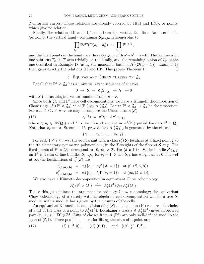
5. Equivariant Chern classes on Qd

Recall that P1 ×Qd has a universal exact sequence of sheaves

0 → S → OnP1×Qd

→ T → 0

with S the tautological vector bundle of rank n− r.Since both Qd and P1 have cell decompositions, we have a Kunneth decomposition of

Chow rings, A∗(P1 ×Qd) ' A∗(P1)⊗Z A∗(Qd). Let π : P1 ×Qd → Qd be the projection.For each 1 ≤ i ≤ n−r we may decompose the Chern class ci(S)

(16) ci(S) = π∗ti + hπ∗ui−1 ,

where ti, ui ∈ Ai(Qd) and h is the class of a point in A1(P1) pulled back to P1 × Qd.Note that u0 = −d. Strømme [16] proved that A∗(Qd)Q is generated by the classes

{t1, . . . , tk, u1, . . . , uk−1} .

For each 1 ≤ i ≤ n−r, the equivariant Chern class cTi (S) localizes at a fixed point p to

the ith elementary symmetric polynomial ei in the T -weights of the fibre of S at p. Thefixed points of P1 ×Qd correspond to {0,∞}×F . For (δ, a,b) ∈ F , the bundle S(δ,a,b)

on P1 is a sum of line bundles Saj ,bjej for δj = 1. Since Sa,b has weight af at 0 and −bf

at ∞, the localizations of cTi (S) are

cTi,0,(δ,a,b) = ei({ej + ajf | δj = 1}) at (0, (δ, a,b))

cTi,∞,(δ,a,b) = ei({ej − bjf | δj = 1}) at (∞, (δ, a,b)) .

We also have a Kunneth decomposition in equivariant Chow cohomology:

A∗T (P1 ×Qd)

∼←−− A∗

T (P1)⊗S A∗T (Qd) .

To see this, just imitate the argument for ordinary Chow cohomology; the equivariantChow cohomology of a variety with an algebraic cell decomposition will be a free S-module, with a module basis given by the closures of the cells.

An equivariant Kunneth decomposition of cTi (S) analogous to (16) requires the choice

of a lift of the class of a point to A1T (P1). Localizing a class x ∈ A1

T (P1) gives an orderedpair (x0, x∞) ∈ Zf ⊕ Zf . Lifts of classes from A1(P1) are only well-defined modulo thespan of (f , f). Three possible choices for lifting the class of a point are:

(17) (i) (−f , 0) , (ii) (0, f) , and (iii) 12(−f , f) .


The symmetric lift (iii) requires rational coefficients. We will use this lift to express ourformulas.

Given a lift h ∈ A1T (P1) of the class of a point, the formula (16) defines equivariant

lifts of the classes ti, ui−1. Strømme’s result together with Proposition 9 implies thatthese classes generate A∗

T (X)Q as an SQ-algebra.

Proposition 19. The symmetric choice (iii) of lift h ∈ A1T (P1) of the class of a point give

the formula for the Kunneth components ti, ui−1 of the equivariant Chern class cTi (S) of

the bundle S. We express this in terms of its localization at the fixed point of Qd indexedby p := (δ, a,b).

ti,p =1

2(cT

i,0,p + cTi,∞,p) ui−1,p =

1

f(cT

i,∞,p − cTi,0,p) .

6. Equivariant Chow ring of the quot scheme Q2(0, 2)

We use Theorem 1 to describe the equivariant Chow ring of Q2 := Q2(0, 2). We firstgive a basis for A∗

T (Q2) as a module over S = Z[e1, e2, f ].

The equivariant Chow ring is the collection of tuples (fp | p ∈ QT2 ) ∈ SQT

2 whichsatisfy the relations of Theorem 1. If p and q are connected by an edge in the momentmultigraph (see Figure 1) with weight χ, then fp − fq lies in the ideal generated by χ.These are the standard GKM relations.

There are two multiedges with four vertices in the multigraph, namely the verticaland horizontal lines of symmetry. They should be seen as flattened quadrangles, sincethey are images of subvarieties isomorphic to P1 × P1. Each gives rise to an additionalrelation, as follows. Suppose that the quadrangle has four vertices a, b, c, d:

-χ a

b

cd(((

hhh

hhh

(((

(Here, the edges are parallel with direction χ.) Then the tuples (fp) must satisfy

fa − fb − fc + fd ∈ χ2S .

These are relations of types II(c)′ (horizontal) and III′ (vertical) of Theorem 1.The remaining multiedges with more than two vertices are the left and right vertical

edges, both with three vertices. They should be seen as flattened triangles, since theycome from subvarieties isomorphic to P2. The additional relations they induce are de-scribed as follows. Let the three fixed points on the multiedge be a, b, c, with b betweena and c. Then

fa − 2fb + fc ∈ f2S .

This is relation of type III′ of Theorem 1.When k = C, we can construct an S-module basis for equivariant cohomology using

equivariant Morse theory; as is well-known, a generic projection of the moment mapto a line will give a Morse function which is perfect for equivariant cohomology. Thisresults in an inductive algorithm to produce a basis, which is nicely expounded in [17](see also [12]). Pick a direction vector v (corresponding to an element of the Lie algebratR) which does not annihilate the direction vector of any edge. Orient each edge to havepositive pairing with v, this is the Hasse diagram of a partial order on the fixed points


induced by v. Then, using the relations described above, we can inductively constructa triangular basis with respect to this ordering. That is, if f = f(p) corresponds to thefixed point p, it vanishes at q (fq = 0) unless p < q, and fp is the product of weightsof edges pointing down from p. While this algorithm was motivated by Morse theory, itmakes sense over any field k, if v is a linear function on the character group of T whichdoes not annihilate any edge of the moment graph.

Set e := e1 − e2 and pick the vector v = f + εe, where ε > 0 is small. One basiselement is the identity f( ), which localizes to 1 at each fixed point. We display eachof the remaining nine in Figure 2 as a localization diagram, writing its localizations ona copy of a moment multigraph.

2f

f−e

f

f+e

f−e f+e

f−e

f

f+e

0f( )

c

¤¤¤º

v

2f

2ff

2f

f f

0f

0

0

c

f( )

f2

f2

0f2

0 0

00

0

0

c

f( )

f(f + e)

0ef

2ef

0 ef

00

0

0

c

f( )

f(f + e)

00

2ef

0 ef

0ef

0

0

c

f( )

0

00

e(e−f)

0 e2

00

e(e+f)

0

c

f( )

f2(f + e)

00

2e2f

0 e2f

00

0

0

c

f( )

f2(f + e)

00

2ef2

0 0

00

0

0

c

f( )

f2(f2 − e2)

00

0

0 0

00

0

0

c

f( )

Figure 2. An S-module basis for A∗T (Q2(0, 2)).


Set x := f( ) − f , y := f( ) − f , and z := f( ) − f( ). Figure 3 shows theirlocalization diagrams. We show that they generate A∗

T (Q2)Q as an SQ-algebra by showing

f

f

0f

0 0

−f

0−f

−fx

f

−e

0e

−e e

−e

0e

−fy

0

0ef

0

0 0

0−ef

0

0z

Figure 3. Generators for the SQ-algebra A∗T (Q2(0, 2))Q.

that each basis element f(p) of degree greater than 2 lies in SQ[x, y, z]. Since

f( ) = 12x(x+f) ,

f( ) = 12(y+e)(y−x) , and(18)

f( ) + f( ) , = (y+e)(x+f) ,

the four degree 2 basis elements lie in SQ[x, y, z]. The remaining three basis elementsalso lie in SQ[x, y, z],

yf( ) = f( ) , xf( ) = f( ) , and (y − e)f( ) = f( ) .

Inspecting the localization diagrams of x, y, and z, shows that the following 5 expres-sions vanish in A∗

T (Q2)

(19) xz , yz , x(x2 − f2) , (y2 − e2)(y − x) , and z2 − (y2 − e2)(x2 − f2) .

In the lexicographic term order where z > y > x > e > f , these five polynomials form aGrobner basis for the ideal I of Q[e1, e2, f , x, y, z] they generate with leading terms xz,yz, x3, y3, and z2. There are ten standard monomials

1, x, y, x2, xy, y2, z, x2y, xy2, and x2y2 .

Since A∗T (Q2)Q is free over SQ = Q[e1, e2, f ] of rank 10, we conclude that

A∗T (Q2)Q ' Q[e1, e2, f , x, y, z]/I .

Using Proposition 9, we obtain the presentation of the rational Chow ring

A∗(Q2)Q ' Q[x, y, z]/〈xz, yz, x3, xy2 − y3, z2 − x2y2〉 .

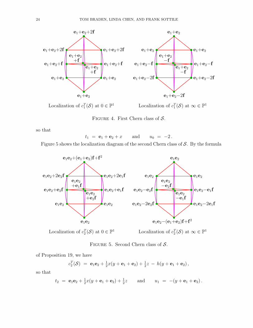
By (18), the integral Chow ring has a more complicated presentation.We now consider Strømme’s generators. Figure 4 shows the localization diagram of

the first Chern class of S. By the formula of Proposition 19, we have

cT1 (S) = e1 + e2 + x − 2h ,


e1+e2+2f

e1+e2+2f e1+e2+2f

e1+e2+f e1+e2+f

e1+e2 e1+e2

e1+e2

+f

e1+e2

+f

e1+e2

Localization of cT1 (S) at 0 ∈ P1

e1+e2

e1+e2 e1+e2

e1+e2−f e1+e2−f

e1+e2−2f e1+e2−2f

e1+e2

−f

e1+e2

−f

e1+e2−2f

Localization of cT1 (S) at ∞ ∈ P1

Figure 4. First Chern class of S.

so that

t1 = e1 + e2 + x and u0 = −2 .

Figure 5 shows the localization diagram of the second Chern class of S. By the formula

e1e2+(e1+e2)f+f2

e1e2+2e2f e1e2+2e1f

e1e2+e2f e1e2+e1f

e1e2 e1e2

e1e2

+e1f

e1e2

+e2f

e1e2

Localization of cT2 (S) at 0 ∈ P1

e1e2

e1e2 e1e2

e1e2−e2f e1e2−e1f

e1e2−2e2f e1e2−2e1f

e1e2−(e1+e2)f+f2

e1e2

−e2f

e1e2

−e1f

Localization of cT2 (S) at ∞ ∈ P1

Figure 5. Second Chern class of S.

of Proposition 19, we have

cT2 (S) = e1e2 + 1

2x(y + e1 + e2) + 1

2z − h(y + e1 + e2) ,

so that

t2 = e1e2 + 12x(y + e1 + e2) + 1

2z and u1 = −(y + e1 + e2) .


The corresponding classes in A∗(Q2) are

t1 = x , u1 = −y , and t2 = 12(z + xy) .

Note that this shows that the claim in [16, Theorem (5.3)] that the classes ti, ui−1 generatethe integral Chow ring is false.

References

[1] Aaron Bertram, Quantum Schubert calculus, Adv. Math. 128 (1997), no. 2, 289–305.[2] Andrzej BiaÃlynicki-Birula, Some theorems on actions of algebraic groups, Ann. of Math. (2) 98

(1973), 480–497.[3] Michel Brion, Equivariant Chow groups for torus actions, Transform. Groups 2 (1997), no. 3, 225–

267.[4] Theodore Chang and Tor Skjelbred, The topological Schur lemma and related results, Ann. of Math.

(2) 100 (1974), 307–321.[5] Dan Edidin and William Graham, Equivariant intersection theory, Invent. Math. 131 (1998), no. 3,

595–634.[6] , Localization in equivariant intersection theory and the Bott residue formula, Amer. J.

Math. 120 (1998), no. 3, 619–636.[7] David Eisenbud, Commutative algebra, Graduate Texts in Mathematics, vol. 150, Springer-Verlag,

New York, 1995.[8] Laurent Evain, The Chow ring of punctual Hilbert schemes of toric surfaces.

arXiv:math.AG/0503697.[9] William Fulton, Intersection theory, second ed., Ergebnisse der Mathematik und ihrer Grenzgebiete.

3. Folge. A Series of Modern Surveys in Mathematics [Results in Mathematics and Related Areas.3rd Series. A Series of Modern Surveys in Mathematics], vol. 2, Springer-Verlag, Berlin, 1998.

[10] Rebecca Goldin and Tara S. Holm, The equivariant cohomology of Hamiltonian G-spaces from

residual S1 actions, Math. Res. Lett. 8 (2001), no. 1-2, 67–77.[11] Mark Goresky, Robert Kottwitz, and Robert MacPherson, Equivariant cohomology, Koszul duality,

and the localization theorem, Invent. Math. 131 (1998), no. 1, 25–83.[12] V. Guillemin and C. Zara, 1-skeleta, Betti numbers, and equivariant cohomology, Duke Math. J.

107 (2001), no. 2, 283–349.[13] Victor Guillemin and Catalin Zara, Combinatorial formulas for products of Thom classes, Geome-

try, mechanics, and dynamics, Springer, New York, 2002, pp. 363–405.[14] , The existence of generating families for the cohomology ring of a graph, Adv. Math. 174

(2003), no. 1, 115–153.[15] Birger Iversen, A fixed point formula for action of tori on algebraic varieties, Invent. Math. 16

(1972), 229–236.[16] Stein Arlid Strømme, On parameterized rational curves in Grassmann varieties, Space Curves

(F. Ghione, C. Peskine, and E. Sernesi, eds.), Lecture Notes in Math., vol. 1266, Springer-Verlag,1987, pp. 251–272.

[17] Julianna S. Tymoczko, An introduction to equivariant cohomology and homology, following Goresky,

Kottwitz, and MacPherson, Snowbird lectures in algebraic geometry, Contemp. Math., vol. 388,Amer. Math. Soc., Providence, RI, 2005, pp. 169–188.


Department of Mathematics, University of Massachusetts, Amherst, MA 01003, USA

E-mail address: [email protected]

Department of Mathematics, The Ohio State University, Columbus, OH 43210, USA


Department of Mathematics, Texas A&M University, College Station, TX 77843,

USA


Documents

30 November 2006. math.AG/0602161sottile/research/pdf/quot.pdf30 November 2006. math.AG/0602161 THE EQUIVARIANT CHOW RINGS OF QUOT SCHEMES TOM BRADEN, LINDA CHEN, AND FRANK SOTTILE