1

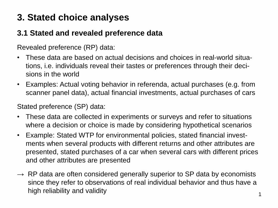
3. Stated choice analyses

3.1 Stated and revealed preference data

Revealed preference (RP) data:

• These data are based on actual decisions and choices in real-world situa-

tions, i.e. individuals reveal their tastes or preferences through their deci-

sions in the world

• Examples: Actual voting behavior in referenda, actual purchases (e.g. from

scanner panel data), actual financial investments, actual purchases of cars

Stated preference (SP) data:

• These data are collected in experiments or surveys and refer to situations

where a decision or choice is made by considering hypothetical scenarios

• Example: Stated WTP for environmental policies, stated financial invest-

ments when several products with different returns and other attributes are

presented, stated purchases of a car when several cars with different prices

and other attributes are presented

→ RP data are often considered generally superior to SP data by economists

since they refer to observations of real individual behavior and thus have a

high reliability and validity

2

However, SP data have several advantages compared with RP data:

• In contrast to RP data, SP data are not limited to situations, products, and

attributes of alternatives that currently exist or have existed in the past, but

can also refer to new products (e.g. new energy sources in vehicles or new

financial products), new attributes of products, or products with a low market

penetration

• Even for already existing situations and products, it is possible that some re-

levant factors and thus explanatory variables have little variability (e.g. pri-

ces of products or interest rates in financial products) so that an econometric

analysis is hardly possible with RP data. Instead, SP experiments can be

designed to contain as much variation in attributes as desired.

• Explanatory variables for real-world decisions can be strongly correlated

(e.g. fuel efficiency and motor power of cars are mostly strongly negatively

correlated, price and quality of cars can be strongly positively correlated),

which makes the econometric analysis with RP data problematic

• The collection of RP data can be very time consuming, very expensive, or

even impossible for specific topics

• In particular, RP data are not or only indirectly available for valuations of

public goods such as environmental goods (e.g. climate protection) since

they are not traded in real economic markets so that e.g. the analysis of

WTP for climate protection is problematic or impossible with RP data

3

Contingent valuation methods (CVM):

• In this SP approach mostly non-market resources (e.g. natural resources),

which typically give some utility, are valued by respondents in a survey

• Typically, respondents are directly asked for the WTP for public goods such

as for a new local recreation area or an improvement in environmental quali-

ty (e.g. an increase in biodiversity)

• The WTP questions in CVM can be based on classical open-ended formats

or several types of (e.g. single or double bounded) binary choice formats

• A problem of CVM is that it strongly relies on the accuracy of the description

of the resources (e.g. local recreation area) that are valued. Furthermore,

CVM cannot value separate components or attributes of the resources.

Conjoint analyses:

• In this non-choice SP approach respondents rank or rate each combination

of components or attributes of several alternatives such as products

• However, such ranking tasks are problematic with respect to utility theory,

which do not necessarily reveal the WTP for some attributes. In particular, in

real-world situations decision makers have to make specific choices (e.g.

between several vehicles).

→ As a consequence, data from stated choice experiments (SCE), where res-

pondents are asked to indicate their preference among two or more multi-

attribute alternatives, are in many situations the most attractive SP data

4

3.2 Design of stated choice experiments

Overview of main components of SCE:

• Problem definition and development, i.e. analysis of the research questions

(e.g. analysis of the possible preferences and WTP for electric vehicles or

for sustainable investments)

• Identification and selection of choice alternatives (e.g. different energy sour-

ces and propulsion technologies in vehicles, different investment products)

including the decision for labeled or unlabeled alternatives

• Selection of attributes, attribute levels, and attribute-level labels

• Selection of experimental design, i.e. specification of how attribute levels are

combined to form different alternatives

• Generation of choice sets, i.e. decision on how the attribute level combina-

tions are blocked for the presentation to the respondents

Challenges in the survey and questionnaire construction (which does not only

comprise an SCE, but also other questions) for reliable econometric analyses:

• Generally, the survey design should strongly conform to the problem defini-

tion and not vice versa, i.e. the research question should not be adjusted to

the survey design

• The questions must correspond to the type of data that are necessary for

the econometric models (e.g. linear or nonlinear) in the empirical analysis

5

• The questions must be appropriate for the study, i.e. questions that are not

used in the econometric analysis unnecessarily extend the length of the sur-

vey (and thus the costs and the efforts for the respondents)

• The questions must be understandable, realistic, and unambiguous for the

respondents and should not be based on specific technical expertise (e.g.

with respect to different energy sources and propulsion technologies in ve-

hicles)

• Biased and leading questions as well as non-mutually exclusive categories

in the SCE should be avoided

• The decision context in the SCE should be clear, i.e. a descriptive story

should be provided that explains the context in which to consider the choice

of the different alternatives (e.g. it should be clarified whether holiday or bu-

siness trips are considered for the choice among different travel modes)

• The survey delivery method must be appropriate, e.g. phone surveys gene-

rally make no sense for SCE since the questions are too complex. While

(computer-assisted) personal interviews are attractive, they can be very ex-

pensive so that recently often online surveys are conducted instead of writ-

ten surveys, which were very attractive in the past.

• Finally, the whole questionnaire should be thoroughly tested before data col-

lection, e.g. on the basis of expert talks, focus groups, and especially pre-

tests with a small sample from the interesting population

6

Hypothetical bias:

In order to circumvent or at least reduce problems through the hypothetical

character of SCE or general SP data (especially the overestimation of WTP),

several ex ante procedures are often included to increase the validity of SCE

data such as cheap talk scripts (e.g. the advice that the income and wealth si-

tuation should be strongly considered in the SCE) or honesty oaths

Labeled and unlabeled SCE:

• Labeled SCE assign specific labels to each alternative (e.g. air, train, bus,

car in travel mode choices or electric, gasoline, diesel cars in the choice

among different energy sources and propulsion technologies in vehicles)

• Unlabeled SCE use generic or uninformative titles or headings for the alter-

natives (e.g. alternative 1, alternative 2, etc.) and thus do not give additional

information to the respondent

• A label for an alternative can be considered like an attribute, which is speci-

fically obvious in quasi-labeled SCE, where each alternative refers to exactly

one specification (e.g. when electric, gasoline, and diesel are included as at-

tribute levels for the attribute energy sources and propulsion technologies)

• One advantage of unlabeled SCE is that they do not require the identifica-

tion and use of all alternatives among the universal set of alternatives

• However, labeled SCE can sometimes be more realistic and also be useful

for the estimation of alternative-specific constants

7

Experimental designs:

• Full factorial design

- Design in which all possible attribute level combinations (which can be dif-

ferently coded) are considered

- Example: For two attributes (e.g. purchase price and CO2 emissions) with

three levels, respectively (e.g. 5000, 10000, 15000 Euro and 0, 100, 200

gram per kilometer) in the case of a vehicle choice, nine (i.e. 3·3) attribute

level combinations for one alternative are possible

- In general, the number of possible attribute level combinations depends

on the number L of attribute levels, the number k2 of attributes, and the

number J of alternatives and thus is Lk2J in labeled SCE and Lk2 in unlabe-

led SCE

- It is important to note that the alternatives in labeled SCE often have diffe-

rent attributes and especially different attribute levels (e.g. 0, 100, 200

gram CO2 emissions per kilometer for electric vehicles, but only 100 and

200 gram for gasoline vehicles)

- Full factorial designs have very attractive statistical properties for parame-

ter estimation and statistical testing, but the number of attribute level com-

binations is mostly too large in practice so that commonly only a fraction

of them is used

8

• Fractional factorial design

- Design in which only a fraction of all possible attribute level combinations

is used

- While it is possible to randomly select a specific number of combinations,

this can lead to inefficient or sub-optimal designs

- Instead, several scientific methods can be used to select more sophistica-

ted optimal attribute level combinations

- One popular approach is the orthogonal fractional factorial design, which

is generated such that the attributes of the design are uncorrelated. How-

ever, the minimization of the correlations in this design generally does not

lead to the statistically most efficient design.

• Optimal or statistically efficient designs

- Optimal designs often allow for correlations across the attributes, but are

statistically efficient

- A popular criterion is the determinant of the variance-covariance matrix of

the parameter vector that is estimated with ML in a model. The maximiza-

tion of this determinant leads to D-optimal designs.

- The value of this determinant (i.e. of the determinant of the inverse of the

variance-covariance matrix) is the basis for the calculation of the level of

D-efficiency

9

Generation and selection of choice sets:

• Each attribute level combination from the experimental design is a separate

potential choice set and thus provides the relevant information about the al-

ternatives, attributes, and attribute levels in the hypothetical scenario

• In each choice set it is important that the attribute levels are well defined and

clear for the respondents so that a mechanism of describing unambiguously

each attribute level is required. One common approach is the inclusion of

pictures (e.g. for the description of colors as attribute for cars).

• It is important to ensure that the decision in each choice set is independent

to the decisions in all other choice sets, i.e. that the hypothetical scenarios in

the choice sets cannot be compared

• Finally, a specific number (e.g. six or 12) of the possible choice sets from the

experimental design must be randomly assigned to the respondents

No choice option:

The decision whether to include the option to not choose an alternative should

be based on the objective of the study. For example, if the demand for different

alternatives in a market is considered, the inclusion of the no choice alternative

is mostly useful, whereas the inclusion of the no choice option can be hindering

in an analysis of the effect of different attribute levels. Without the no choice al-

ternative, the analyzed decision is a conditional choice, i.e. conditional on

choosing any alternative.

10

It is often (especially in the case of the valuation of public goods) useful to in-

clude the status quo (i.e. baseline) alternative besides other alternatives:

• In some cases, the inclusion of the status quo alternative as additional alter-

native represents an inclusion of RP data in SCE (e.g. in the choice among

different electricity tariffs, the current electricity tariff can be included)

• The information of the current status quo alternative must be collected be-

fore the SCE in the survey so that it can be included in the experiment •

• In contrast to the other alternatives, the status quo alternative and its attri-

bute levels remain constant across all choice sets for the same respondent

• The individual attribute levels are often coordinated with the levels in the sta-

tus quo to make the hypothetical scenarios more realistic for the respondent

(e.g. the electricity costs as an attribute in the choice among different electri-

city tariffs can be very different across households)

• These customized attribute levels (which need not refer to the inclusion of

the status quo alternative) are mostly based on percentage changes from

the status quo levels (e.g. -10%, 0%, +10% of the current electricity costs)

• Commonly, not the percentage changes, but the respective values that are

linked with the percentage changes are presented in the choice sets (e.g.

550 Euro instead of +10%, when 500 Euro is the cost value in the status

quo), which can lead to very different values across the respondents

• However, the percentage changes instead of these values should be used in

the econometric analysis and thus e.g. for the WTP estimation

11

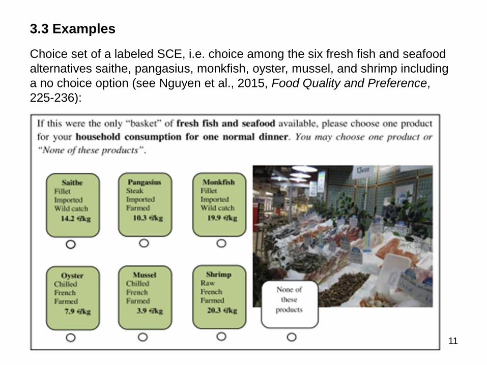
3.3 Examples

Choice set of a labeled SCE, i.e. choice among the six fresh fish and seafood

alternatives saithe, pangasius, monkfish, oyster, mussel, and shrimp including

a no choice option (see Nguyen et al., 2015, Food Quality and Preference,

225-236):

12

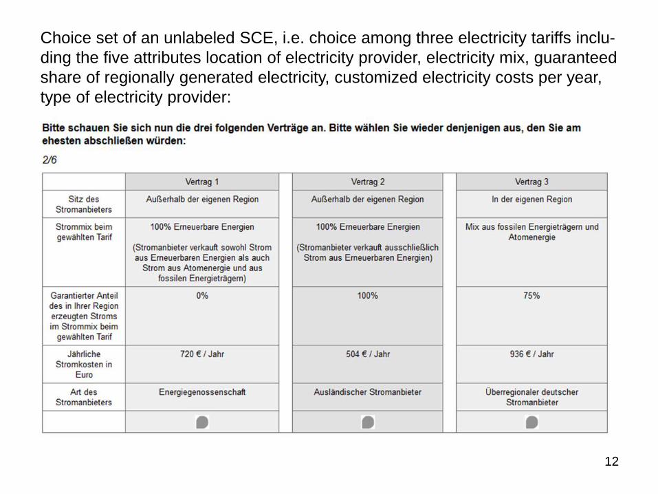
Choice set of an unlabeled SCE, i.e. choice among three electricity tariffs inclu-

ding the five attributes location of electricity provider, electricity mix, guaranteed

share of regionally generated electricity, customized electricity costs per year,

type of electricity provider:

13

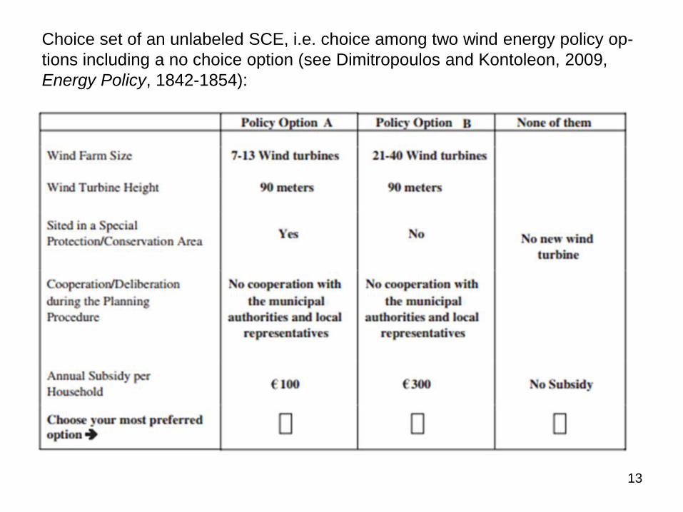
Choice set of an unlabeled SCE, i.e. choice among two wind energy policy op-

tions including a no choice option (see Dimitropoulos and Kontoleon, 2009,

Energy Policy, 1842-1854):

14

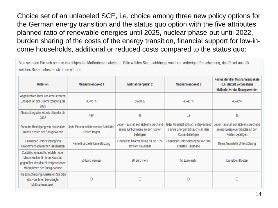
Choice set of an unlabeled SCE, i.e. choice among three new policy options for

the German energy transition and the status quo option with the five attributes

planned ratio of renewable energies until 2025, nuclear phase-out until 2022,

burden sharing of the costs of the energy transition, financial support for low-in-

come households, additional or reduced costs compared to the status quo:

15

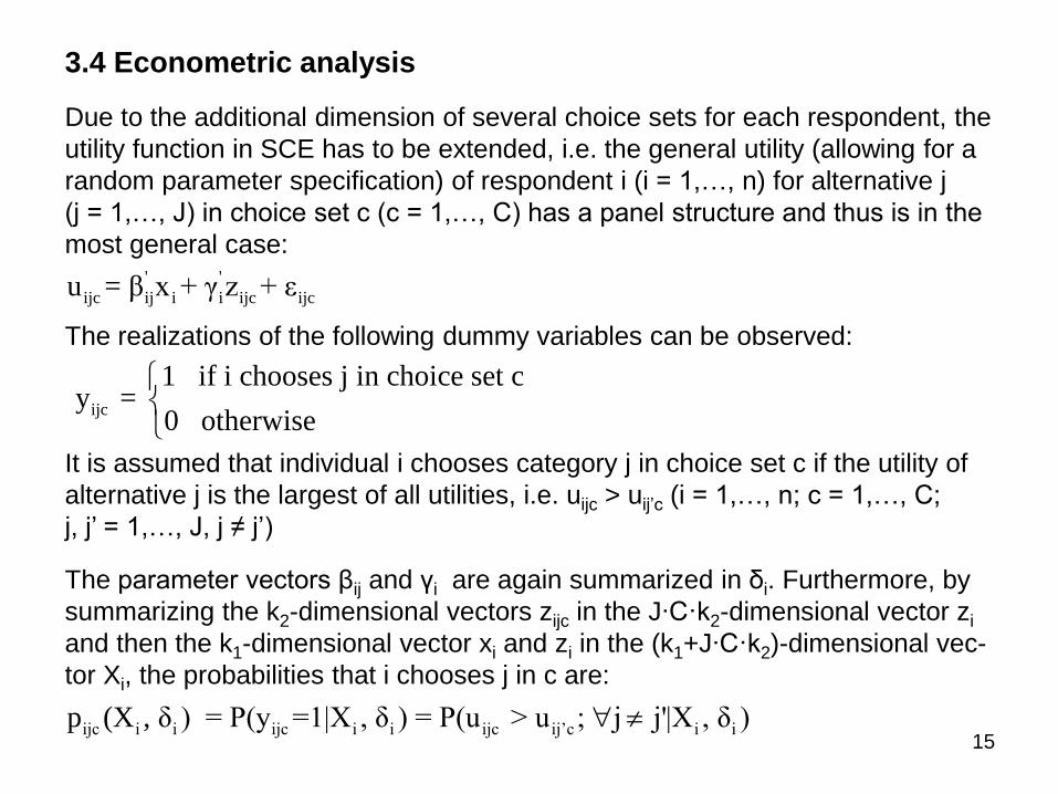
3.4 Econometric analysis

Due to the additional dimension of several choice sets for each respondent, the

utility function in SCE has to be extended, i.e. the general utility (allowing for a

random parameter specification) of respondent i (i = 1,…, n) for alternative j

(j = 1,…, J) in choice set c (c = 1,…, C) has a panel structure and thus is in the

most general case:

The realizations of the following dummy variables can be observed:

It is assumed that individual i chooses category j in choice set c if the utility of

alternative j is the largest of all utilities, i.e. uijc > uij’c (i = 1,…, n; c = 1,…, C;

j, j’ = 1,…, J, j ≠ j’)

The parameter vectors βij and γi are again summarized in δi. Furthermore, by

summarizing the k2-dimensional vectors zijc in the J∙C·k2-dimensional vector zi

and then the k1-dimensional vector xi and zi in the (k1+J∙C·k2)-dimensional vec-

tor Xi, the probabilities that i chooses j in c are:

' '

ijc ij i i ijc ijcu = β x + γ z + ε

ijc

1 if i chooses j in choice set cy =

0 otherwise

ijc i i ijc i i ijc ij’c i ip (X , δ ) = P(y =1|X , δ ) = P(u > u ; j j'|X , δ )

16

Multinomial logit models:

• In this case, the parameter vectors βij and γi are fixed so that it follows for

the utility function:

• The βj are again summarized in the J∙k2-dimensional vector β. The assump-

tion that the error terms εijc are independently and identically standard ex-

treme value distributed over all j = 1,…, J and all c = 1,…, C (and naturally

over also all i = 1,…, n) leads to the following choice probabilities:

• It follows for the log-likelihood function and the ML estimator:

• However, the use of multinomial logit models on the basis of SCE data is

even more restrictive since they do not only assume independence of the

error terms over the J alternatives, but also over the C choice sets

' '

ijc j i ijc ijcu = β x + γ z + ε

'j i ijc

'm i imc

β x + γ'z

ijc i ijc i Jβ x + γ'z

m=1

ep (X , β, γ) = P(y =1|X , β, γ) =

e

n J C

ijc ijc i

i=1 j=1 c=1

n J C

ML ijc ijc iθ

i=1 j=1 c=1

logL(θ) = y logp (X , β, γ)

θ̂ = arg max y logp (X , β, γ)

17

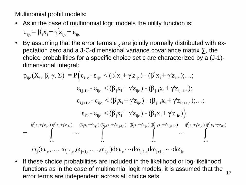
Multinomial probit models:

• As in the case of multinomial logit models the utility function is:

• By assuming that the error terms εijc are jointly normally distributed with ex-

pectation zero and a J·C-dimensional variance covariance matrix ∑, the

choice probabilities for a specific choice set c are characterized by a (J-1)-

dimensional integral:

• If these choice probabilities are included in the likelihood or log-likelihood

functions as in the case of multinomial logit models, it is assumed that the

error terms are independent across all choice sets

' '

ijc j i ijc ijcu = β x + γ z + ε

' '

ijc i i1c ijc j i ijc 1 i i1c

' '

i,j-1,c ijc j i ijc j-1 i i,j-1,c

i,j+1,c

p (X , β, γ, ) = P ε - ε < (β x + γ'z ) - (β x + γ'z );…;

ε - ε < (β x + γ'z ) - (β x + γ'z );

ε

' ' ' 'j i ijc 1 i i1c j i ijc j+1 i i,j+

' '

ijc j i ijc j+1 i i,j+1,c

' '

iJc ijc j i ijc J i iJc

(β x +γ'z )-(β x +γ'z ) (β x +γ'z )-(β x +γ'z

- -

- ε < (β x + γ'z ) - (β x + γ'z );…;

ε - ε < (β x + γ'z ) - (β x + γ'z )

' ' ' 'j i ijc j-1 i i,j-1,c 1,c j i ijc J i iJc(β x +γ'z )-(β x +γ'z ) ) (β x +γ'z )-(β x +γ'z )

- -

j 1c j-1,c j+1,c J,c 1c j-1,c j+1,c Jc φ (ω ,…, ω ,ω ,…,ω )dω dω dω dω

18

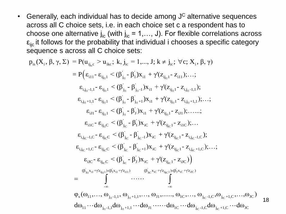
• Generally, each individual has to decide among JC alternative sequences

across all C choice sets, i.e. in each choice set c a respondent has to

choose one alternative jic (with jic = 1,…, J). For flexible correlations across

εijc it follows for the probability that individual i chooses a specific category

sequence s across all C choice sets:

ic

i1 i1 i1

i1

is i ij c ikc ic ic i

' '

i11 ij 1 j 1 i1 ij 1 i11

i,j -1,1

p (X , β, γ, ) = P(u > u ; k, j = 1,..., J; k j ; c; X , β, γ)

= P ε - ε < (β - β )x + γ'(z - z );…;

ε - ε

i1 i1 i1 i1 i1

i1 i1 i1 i1 i1 i1

i1

' '

ij 1 j j -1 i1 ij 1 i,j -1,1

' '

i,j +1,1 ij 1 j j +1 i1 ij 1 i,j +1,1

iJ1 ij 1 j

< (β - β )x + γ'(z - z );

ε - ε < (β - β )x + γ'(z - z );…;

ε - ε < (βi1 i1

i1 iC iC

iC iC iC iC iC

' '

J i1 ij 1 iJ1

' '

i1C ij C j 1 iC ij 1 i1C

' '

i,j -1,C ij C j j -1 iC ij 1

- β )x + γ'(z - z );…...;

ε - ε < (β - β )x + γ'(z - z );…

ε - ε < (β - β )x + γ'(z

iC

iC iC iC iC iC iC

iC iC iC

i,j -1,C

' '

i,j +1,C ij C j j +1 iC ij 1 i,j +1,C

' '

iJC ij C j J iC ij 1 iJC

- z );

ε - ε < (β - β )x + γ'(z - z );…;

ε - ε < (β - β )x + γ'(z - z )

' '' 'j iC ij 1 J iC iJCj i1 ij 1 1 i1 i11 iC iCi1 i1

i1 i1 iC iC

(β x +γ'z )-(β x +γ'z )(β x +γ'z )-(β x +γ'z )

- -

s 11 j -1,1 j +1,1 J1 1C j -1,C j +1,C JC

φ (ω ,…, ω , ω ,…, ω ,......, ω ,…, ω ,ω ,…,ω )

i1 i1 iC iC11 j -1,1 j +1,1 J1 1C j -1,C j +1,C JC dω dω dω dω dω dω dω dω

19

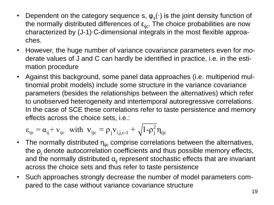
• Dependent on the category sequence s, φs(∙) is the joint density function of

the normally distributed differences of εijc. The choice probabilities are now

characterized by (J-1)∙C-dimensional integrals in the most flexible approa-

ches.

• However, the huge number of variance covariance parameters even for mo-

derate values of J and C can hardly be identified in practice, i.e. in the esti-

mation procedure

• Against this background, some panel data approaches (i.e. multiperiod mul-

tinomial probit models) include some structure in the variance covariance

parameters (besides the relationships between the alternatives) which refer

to unobserved heterogeneity and intertemporal autoregressive correlations.

In the case of SCE these correlations refer to taste persistence and memory

effects across the choice sets, i.e.:

• The normally distributed ηijc comprise correlations between the alternatives,

the ρj denote autocorrelation coefficients and thus possible memory effects,

and the normally distributed αij represent stochastic effects that are invariant

across the choice sets and thus refer to taste persistence

• Such approaches strongly decrease the number of model parameters com-

pared to the case without variance covariance structure

ijc ij ijc

2ijc j i,j,c-1 j ijc ε = α + v with v = ρ v + 1-ρ η

20

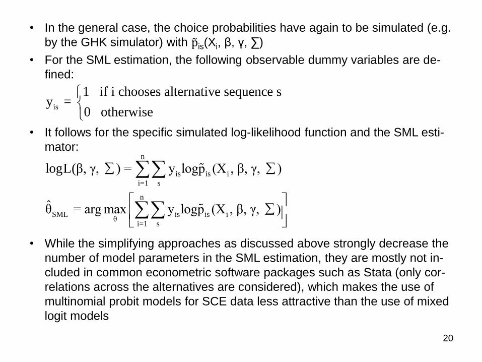
• In the general case, the choice probabilities have again to be simulated (e.g.

by the GHK simulator) with p is(Xi, β, γ, ∑)

• For the SML estimation, the following observable dummy variables are de-

fined:

• It follows for the specific simulated log-likelihood function and the SML esti-

mator:

• While the simplifying approaches as discussed above strongly decrease the

number of model parameters in the SML estimation, they are mostly not in-

cluded in common econometric software packages such as Stata (only cor-

relations across the alternatives are considered), which makes the use of

multinomial probit models for SCE data less attractive than the use of mixed

logit models

n

is is i

i=1 s

n

SML is is iθ

i=1 s

logL(β, γ, ) = y logp (X , β, γ, )

θ̂ = arg max y logp (X , β, γ, )

is

1 if i chooses alternative sequence sy =

0 otherwise

21

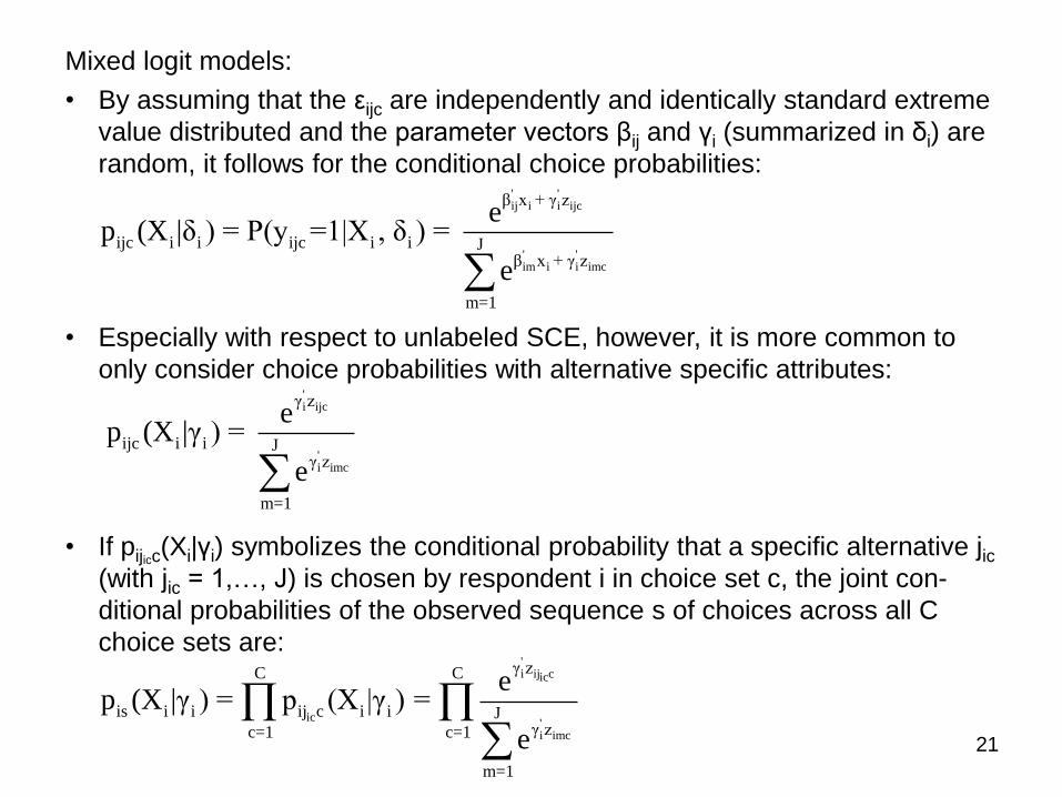
Mixed logit models:

• By assuming that the εijc are independently and identically standard extreme

value distributed and the parameter vectors βij and γi (summarized in δi) are

random, it follows for the conditional choice probabilities:

• Especially with respect to unlabeled SCE, however, it is more common to

only consider choice probabilities with alternative specific attributes:

• If pijicc

(Xi|γi) symbolizes the conditional probability that a specific alternative jic

(with jic = 1,…, J) is chosen by respondent i in choice set c, the joint con-

ditional probabilities of the observed sequence s of choices across all C

choice sets are:

' 'ij i i ijc

' 'im i i imc

β x + γ z

ijc i i ijc i i Jβ x + γ z

m=1

ep (X |δ ) = P(y =1|X , δ ) =

e

'i ij cic

ic'i imc

γ zC C

is i i ij c i i Jγ zc=1 c=1

m=1

ep (X |γ ) = p (X |γ ) =

e

'i ijc

'i imc

γ z

ijc i i Jγ z

m=1

ep (X |γ ) =

e

22

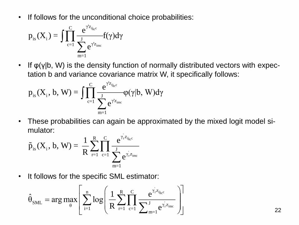
• If follows for the unconditional choice probabilities:

• If φ(γ|b, W) is the density function of normally distributed vectors with expec-

tation b and variance covariance matrix W, it specifically follows:

• These probabilities can again be approximated by the mixed logit model si-

mulator:

• It follows for the specific SML estimator:

ij cic

imc

γ'zC

is i Jγ'zc=1

m=1

ep (X ) = f(γ)dγ

e

ij cic

imc

γ'zC

is i Jγ'zc=1

m=1

ep (X , b, W) = φ(γ|b, W)dγ

e

'r ij cic

'r imc

γ zCR

is i Jγ zr=1 c=1

m=1

1 ep (X , b, W) =

Re

'r ij cic

'r imc

γ zCn R

SML J γ zθi=1 r=1 c=1

m=1

1 eθ̂ arg max log

R e

23

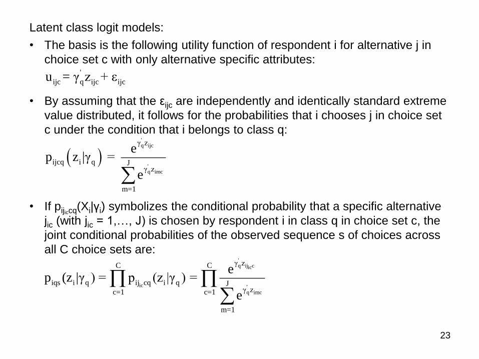
Latent class logit models:

• The basis is the following utility function of respondent i for alternative j in

choice set c with only alternative specific attributes:

• By assuming that the εijc are independently and identically standard extreme

value distributed, it follows for the probabilities that i chooses j in choice set

c under the condition that i belongs to class q:

• If pijiccq(Xi|γi) symbolizes the conditional probability that a specific alternative

jic (with jic = 1,…, J) is chosen by respondent i in class q in choice set c, the

joint conditional probabilities of the observed sequence s of choices across

all C choice sets are:

'

ijc q ijc ijcu = γ z + ε

'q ijc

'q imc

γ z

ijcq q J

m=

iγ z

1

ze

p |γ =

e

'q ij cic

ic 'q imc

γ zC C

iqs i q ij cq i q Jγ zc=1 c=1

m=1

ep (z |γ ) = p (z |γ ) =

e

24

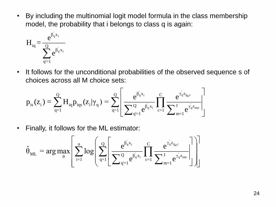
• By including the multinomial logit model formula in the class membership

model, the probability that i belongs to class q is again:

• It follows for the unconditional probabilities of the observed sequence s of

choices across all M choice sets:

• Finally, it follows for the ML estimator:

'q i

'q' i

β x

iq Qβ x

q'=1

eH =

e

''q ij cq i ic

' 'q' i q imc

γ zβ xQ Q C

is i iq iqs i q Q Jβ x γ zq=1 q=1 c=1

q'=1 m=1

e ep (z ) = H p (z |γ ) =

e e

''q ij cq i ic

' 'q' i q imc

γ zβ xQ Cn

ML Q Jβ x γ zθi=1 q=1 c=1

q'=1 m=1

e eθ̂ = arg max log

e e

25

3.5 Applications

---------------------------------------------------------------------------------------------------------

Example 1: Energy sources and propulsion technologies in vehicles (I)

In Ziegler (2012), an SCE (that is based on a computer-randomized fractional

factorial design) with respect to the preferences for alternative energy sources

or propulsion technologies in vehicles is examined:

• The data stem from Computer Assisted Personal Interviews (CAPI), conduc-

ted in selected car dealerships and technical inspection agencies (TÜV) bet-

ween August 2007 and March 2008

• 598 persons from the population of German residents with valid drivers’ li-

censes, who intend or at least could imagine to purchase a vehicle in the

near future, participated in the survey

• The people were asked for details (e.g. size, motor power) of the currently

used and future vehicle as well as for socio-demographic variables (e.g.

age, gender, education)

• The SCE comprises six choice sets with seven hypothetical vehicles types

• It is a quasi-labeled experiment, i.e. each of the seven vehicles refers to

exactly one energy source or propulsion technology

• The vehicles were additionally characterized by five attributes

---------------------------------------------------------------------------------------------------------

26

---------------------------------------------------------------------------------------------------------

Example 1: Energy sources and propulsion technologies in vehicles (II)

Alternatives:

• Gasoline

• Diesel

• Hybrid

• Gas (i.e. natural gas, liquid petroleum gas)

• Biofuel

• Hydrogen

• Electric

Further attributes:

• Purchase price (in Euro)

• Motor power (in horsepower)

• Fuel costs (in Euro per 100 kilometers)

• CO2 emissions (in gram per kilometer)

• Service station availability (in % of stations with respective fuel)

---------------------------------------------------------------------------------------------------------

27

---------------------------------------------------------------------------------------------------------

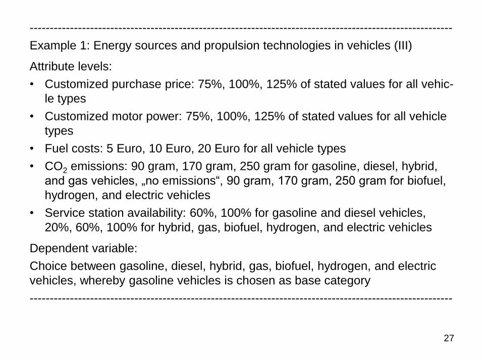
Example 1: Energy sources and propulsion technologies in vehicles (III)

Attribute levels:

• Customized purchase price: 75%, 100%, 125% of stated values for all vehic-

le types

• Customized motor power: 75%, 100%, 125% of stated values for all vehicle

types

• Fuel costs: 5 Euro, 10 Euro, 20 Euro for all vehicle types

• CO2 emissions: 90 gram, 170 gram, 250 gram for gasoline, diesel, hybrid,

and gas vehicles, „no emissions“, 90 gram, 170 gram, 250 gram for biofuel,

hydrogen, and electric vehicles

• Service station availability: 60%, 100% for gasoline and diesel vehicles,

20%, 60%, 100% for hybrid, gas, biofuel, hydrogen, and electric vehicles

Dependent variable:

Choice between gasoline, diesel, hybrid, gas, biofuel, hydrogen, and electric

vehicles, whereby gasoline vehicles is chosen as base category

---------------------------------------------------------------------------------------------------------

28

---------------------------------------------------------------------------------------------------------

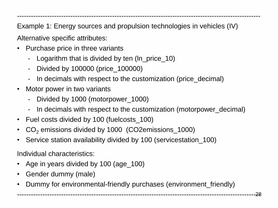
Example 1: Energy sources and propulsion technologies in vehicles (IV)

Alternative specific attributes:

• Purchase price in three variants

- Logarithm that is divided by ten (ln_price_10)

- Divided by 100000 (price_100000)

- In decimals with respect to the customization (price_decimal)

• Motor power in two variants

- Divided by 1000 (motorpower_1000)

- In decimals with respect to the customization (motorpower_decimal)

• Fuel costs divided by 100 (fuelcosts_100)

• CO2 emissions divided by 1000 (CO2emissions_1000)

• Service station availability divided by 100 (servicestation_100)

Individual characteristics:

• Age in years divided by 100 (age_100)

• Gender dummy (male)

• Dummy for environmental-friendly purchases (environment_friendly)

---------------------------------------------------------------------------------------------------------

29

---------------------------------------------------------------------------------------------------------

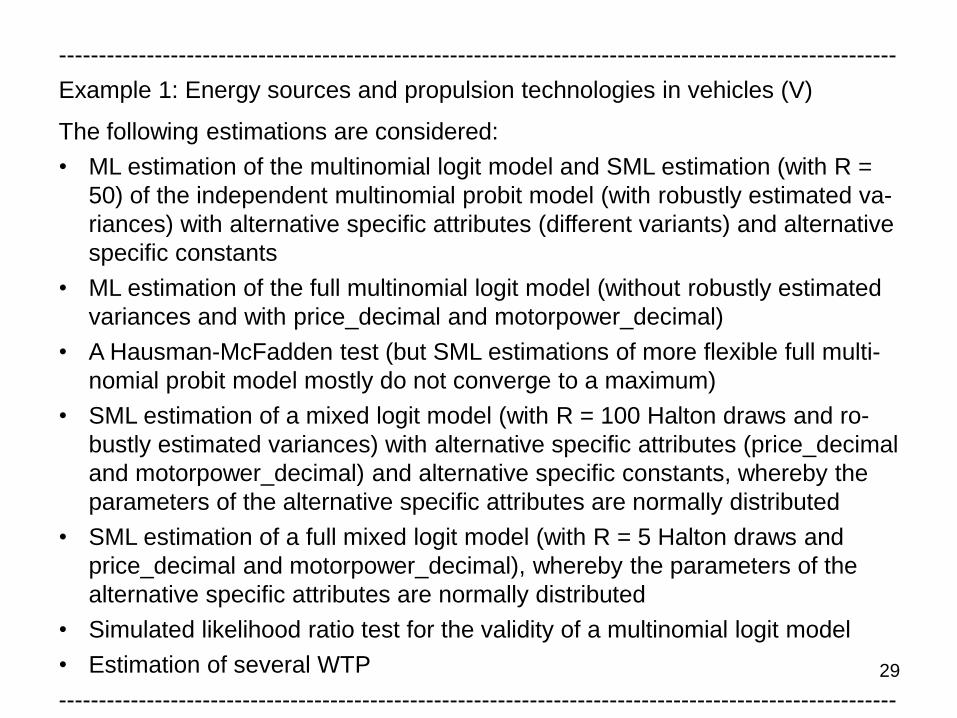
Example 1: Energy sources and propulsion technologies in vehicles (V)

The following estimations are considered:

• ML estimation of the multinomial logit model and SML estimation (with R =

50) of the independent multinomial probit model (with robustly estimated va-

riances) with alternative specific attributes (different variants) and alternative

specific constants

• ML estimation of the full multinomial logit model (without robustly estimated

variances and with price_decimal and motorpower_decimal)

• A Hausman-McFadden test (but SML estimations of more flexible full multi-

nomial probit model mostly do not converge to a maximum)

• SML estimation of a mixed logit model (with R = 100 Halton draws and ro-

bustly estimated variances) with alternative specific attributes (price_decimal

and motorpower_decimal) and alternative specific constants, whereby the

parameters of the alternative specific attributes are normally distributed

• SML estimation of a full mixed logit model (with R = 5 Halton draws and

price_decimal and motorpower_decimal), whereby the parameters of the

alternative specific attributes are normally distributed

• Simulated likelihood ratio test for the validity of a multinomial logit model

• Estimation of several WTP

---------------------------------------------------------------------------------------------------------

30

---------------------------------------------------------------------------------------------------------

Example 1: Energy sources and propulsion technologies in vehicles (VI) asclogit choice ln_price_10 motorpower_1000 fuelcosts_100 CO2emissions_1000 servicestation_100, case(choiceset)

alternatives(alternatives) base(gasoline) robust

Alternative-specific conditional logit Number of obs = 25116

Case variable: id Number of cases = 3588

Alternative variable: alternatives Alts per case: min = 7

avg = 7.0

max = 7

Wald chi2(5) = 1089.75

Log pseudolikelihood = -6115.5597 Prob > chi2 = 0.0000

(Std. Err. adjusted for clustering on id)

------------------------------------------------------------------------------------

| Robust

choice | Coef. Std. Err. z P>|z| [95% Conf. Interval]

-------------------+----------------------------------------------------------------

alternatives |

ln_price_10 | -9.062862 .8571563 -10.57 0.000 -10.74286 -7.382866

motorpower_1000 | 5.812731 .6468658 8.99 0.000 4.544897 7.080564

fuelcosts_100 | -7.572525 .3310998 -22.87 0.000 -8.221469 -6.923582

CO2emissions_1000 | -4.124374 .2819872 -14.63 0.000 -4.677058 -3.571689

servicestation_100 | 1.223938 .0605655 20.21 0.000 1.105232 1.342644

-------------------+----------------------------------------------------------------

biofuel |

_cons | -.6321688 .0707488 -8.94 0.000 -.7708339 -.4935037

-------------------+----------------------------------------------------------------

diesel |

_cons | .0872432 .0549861 1.59 0.113 -.0205276 .195014

-------------------+----------------------------------------------------------------

electric |

_cons | -.9236439 .075934 -12.16 0.000 -1.072472 -.774816

-------------------+----------------------------------------------------------------

gas |

_cons | -.2111685 .0645051 -3.27 0.001 -.3375962 -.0847409

-------------------+----------------------------------------------------------------

gasoline | (base alternative)

-------------------+----------------------------------------------------------------

hybrid |

_cons | -.1579636 .0633328 -2.49 0.013 -.2820935 -.0338336

-------------------+----------------------------------------------------------------

hydrogen |

_cons | -.3168433 .0657563 -4.82 0.000 -.4457232 -.1879633

------------------------------------------------------------------------------------

---------------------------------------------------------------------------------------------------------

31

---------------------------------------------------------------------------------------------------------

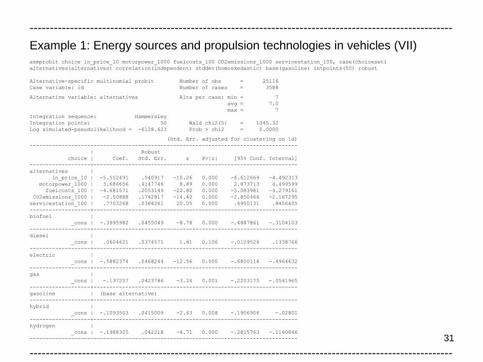
Example 1: Energy sources and propulsion technologies in vehicles (VII) asmprobit choice ln_price_10 motorpower_1000 fuelcosts_100 CO2emissions_1000 servicestation_100, case(choiceset)

alternatives(alternatives) correlation(independent) stddev(homoskedastic) base(gasoline) intpoints(50) robust

Alternative-specific multinomial probit Number of obs = 25116

Case variable: id Number of cases = 3588

Alternative variable: alternatives Alts per case: min = 7

avg = 7.0

max = 7

Integration sequence: Hammersley

Integration points: 50 Wald chi2(5) = 1045.32

Log simulated-pseudolikelihood = -6128.623 Prob > chi2 = 0.0000

(Std. Err. adjusted for clustering on id)

------------------------------------------------------------------------------------

| Robust

choice | Coef. Std. Err. z P>|z| [95% Conf. Interval]

-------------------+----------------------------------------------------------------

alternatives |

ln_price_10 | -5.552491 .540917 -10.26 0.000 -6.612669 -4.492313

motorpower_1000 | 3.686656 .4147746 8.89 0.000 2.873713 4.499599

fuelcosts_100 | -4.681571 .2053149 -22.80 0.000 -5.083981 -4.279161

CO2emissions_1000 | -2.50888 .1742817 -14.40 0.000 -2.850466 -2.167295

servicestation_100 | .7703268 .0384261 20.05 0.000 .6950131 .8456405

-------------------+----------------------------------------------------------------

biofuel |

_cons | -.3995982 .0455049 -8.78 0.000 -.4887861 -.3104103

-------------------+----------------------------------------------------------------

diesel |

_cons | .0604621 .0374571 1.61 0.106 -.0129524 .1338766

-------------------+----------------------------------------------------------------

electric |

_cons | -.5882374 .0468244 -12.56 0.000 -.6800116 -.4964632

-------------------+----------------------------------------------------------------

gas |

_cons | -.137257 .0423786 -3.24 0.001 -.2203175 -.0541965

-------------------+----------------------------------------------------------------

gasoline | (base alternative)

-------------------+----------------------------------------------------------------

hybrid |

_cons | -.1093503 .0415009 -2.63 0.008 -.1906906 -.02801

-------------------+----------------------------------------------------------------

hydrogen |

_cons | -.1988305 .042218 -4.71 0.000 -.2815763 -.1160846

------------------------------------------------------------------------------------

---------------------------------------------------------------------------------------------------------

32

---------------------------------------------------------------------------------------------------------

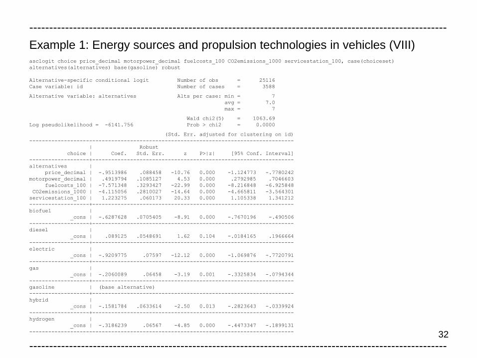
Example 1: Energy sources and propulsion technologies in vehicles (VIII) asclogit choice price_decimal motorpower_decimal fuelcosts_100 CO2emissions_1000 servicestation_100, case(choiceset)

alternatives(alternatives) base(gasoline) robust

Alternative-specific conditional logit Number of obs = 25116

Case variable: id Number of cases = 3588

Alternative variable: alternatives Alts per case: min = 7

avg = 7.0

max = 7

Wald chi2(5) = 1063.69

Log pseudolikelihood = -6141.756 Prob > chi2 = 0.0000

(Std. Err. adjusted for clustering on id)

------------------------------------------------------------------------------------

| Robust

choice | Coef. Std. Err. z P>|z| [95% Conf. Interval]

-------------------+----------------------------------------------------------------

alternatives |

price_decimal | -.9513986 .088458 -10.76 0.000 -1.124773 -.7780242

motorpower_decimal | .4919794 .1085127 4.53 0.000 .2792985 .7046603

fuelcosts_100 | -7.571348 .3293427 -22.99 0.000 -8.216848 -6.925848

CO2emissions_1000 | -4.115056 .2810027 -14.64 0.000 -4.665811 -3.564301

servicestation_100 | 1.223275 .060173 20.33 0.000 1.105338 1.341212

-------------------+----------------------------------------------------------------

biofuel |

_cons | -.6287628 .0705405 -8.91 0.000 -.7670196 -.490506

-------------------+----------------------------------------------------------------

diesel |

_cons | .089125 .0548691 1.62 0.104 -.0184165 .1966664

-------------------+----------------------------------------------------------------

electric |

_cons | -.9209775 .07597 -12.12 0.000 -1.069876 -.7720791

-------------------+----------------------------------------------------------------

gas |

_cons | -.2060089 .06458 -3.19 0.001 -.3325834 -.0794344

-------------------+----------------------------------------------------------------

gasoline | (base alternative)

-------------------+----------------------------------------------------------------

hybrid |

_cons | -.1581784 .0633614 -2.50 0.013 -.2823643 -.0339924

-------------------+----------------------------------------------------------------

hydrogen |

_cons | -.3186239 .06567 -4.85 0.000 -.4473347 -.1899131

------------------------------------------------------------------------------------

---------------------------------------------------------------------------------------------------------

33

---------------------------------------------------------------------------------------------------------

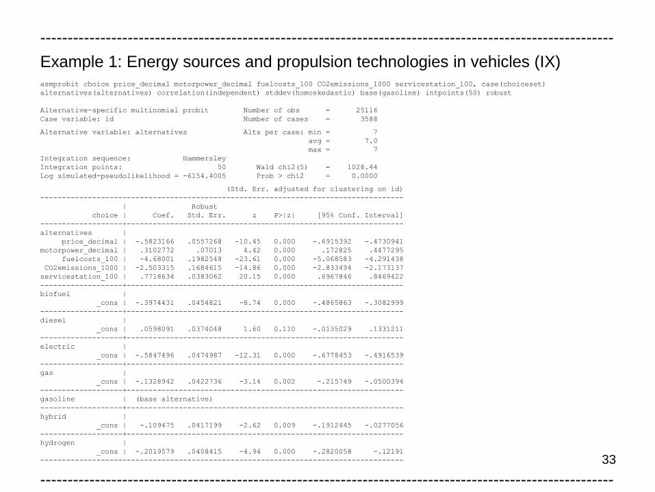
Example 1: Energy sources and propulsion technologies in vehicles (IX) asmprobit choice price_decimal motorpower_decimal fuelcosts_100 CO2emissions_1000 servicestation_100, case(choiceset)

alternatives(alternatives) correlation(independent) stddev(homoskedastic) base(gasoline) intpoints(50) robust

Alternative-specific multinomial probit Number of obs = 25116

Case variable: id Number of cases = 3588

Alternative variable: alternatives Alts per case: min = 7

avg = 7.0

max = 7

Integration sequence: Hammersley

Integration points: 50 Wald chi2(5) = 1028.44

Log simulated-pseudolikelihood = -6154.4005 Prob > chi2 = 0.0000

(Std. Err. adjusted for clustering on id)

------------------------------------------------------------------------------------

| Robust

choice | Coef. Std. Err. z P>|z| [95% Conf. Interval]

-------------------+----------------------------------------------------------------

alternatives |

price_decimal | -.5823166 .0557268 -10.45 0.000 -.6915392 -.4730941

motorpower_decimal | .3102772 .07013 4.42 0.000 .172825 .4477295

fuelcosts_100 | -4.68001 .1982548 -23.61 0.000 -5.068583 -4.291438

CO2emissions_1000 | -2.503315 .1684615 -14.86 0.000 -2.833494 -2.173137

servicestation_100 | .7718634 .0383062 20.15 0.000 .6967846 .8469422

-------------------+----------------------------------------------------------------

biofuel |

_cons | -.3974431 .0454821 -8.74 0.000 -.4865863 -.3082999

-------------------+----------------------------------------------------------------

diesel |

_cons | .0598091 .0374048 1.60 0.110 -.0135029 .1331211

-------------------+----------------------------------------------------------------

electric |

_cons | -.5847496 .0474987 -12.31 0.000 -.6778453 -.4916539

-------------------+----------------------------------------------------------------

gas |

_cons | -.1328942 .0422736 -3.14 0.002 -.215749 -.0500394

-------------------+----------------------------------------------------------------

gasoline | (base alternative)

-------------------+----------------------------------------------------------------

hybrid |

_cons | -.109475 .0417199 -2.62 0.009 -.1912445 -.0277056

-------------------+----------------------------------------------------------------

hydrogen |

_cons | -.2019579 .0408415 -4.94 0.000 -.2820058 -.12191

------------------------------------------------------------------------------------

---------------------------------------------------------------------------------------------------------

34

---------------------------------------------------------------------------------------------------------

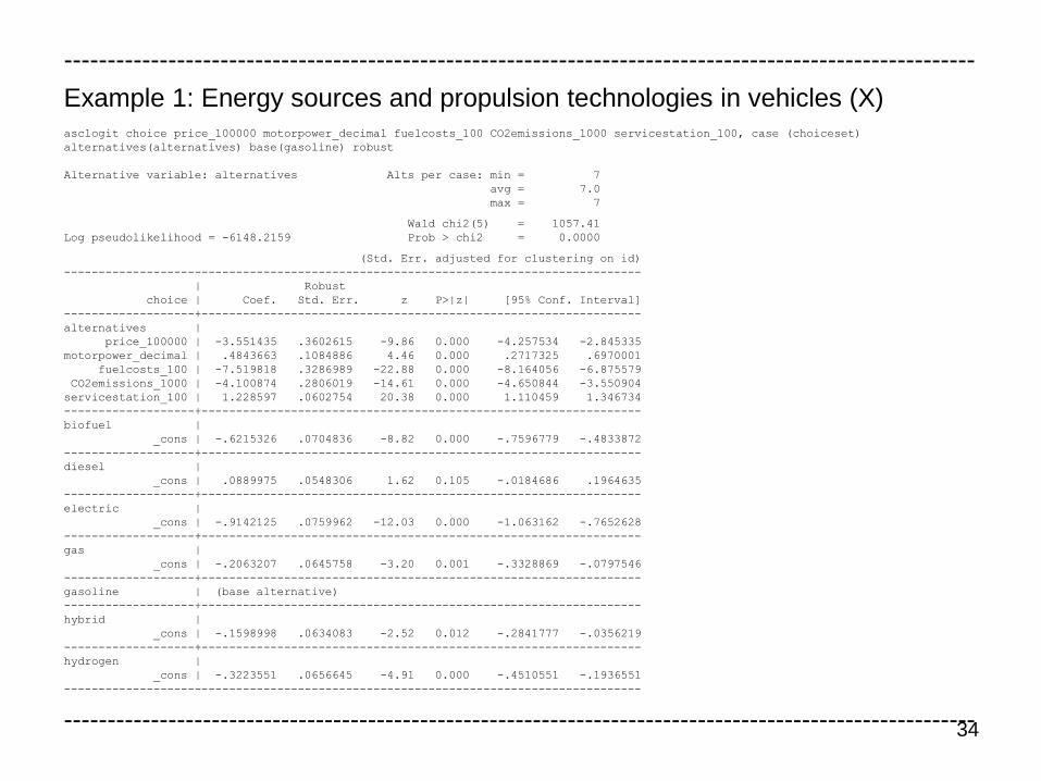
Example 1: Energy sources and propulsion technologies in vehicles (X) asclogit choice price_100000 motorpower_decimal fuelcosts_100 CO2emissions_1000 servicestation_100, case (choiceset)

alternatives(alternatives) base(gasoline) robust

Alternative variable: alternatives Alts per case: min = 7

avg = 7.0

max = 7

Wald chi2(5) = 1057.41

Log pseudolikelihood = -6148.2159 Prob > chi2 = 0.0000

(Std. Err. adjusted for clustering on id)

------------------------------------------------------------------------------------

| Robust

choice | Coef. Std. Err. z P>|z| [95% Conf. Interval]

-------------------+----------------------------------------------------------------

alternatives |

price_100000 | -3.551435 .3602615 -9.86 0.000 -4.257534 -2.845335

motorpower_decimal | .4843663 .1084886 4.46 0.000 .2717325 .6970001

fuelcosts_100 | -7.519818 .3286989 -22.88 0.000 -8.164056 -6.875579

CO2emissions_1000 | -4.100874 .2806019 -14.61 0.000 -4.650844 -3.550904

servicestation_100 | 1.228597 .0602754 20.38 0.000 1.110459 1.346734

-------------------+----------------------------------------------------------------

biofuel |

_cons | -.6215326 .0704836 -8.82 0.000 -.7596779 -.4833872

-------------------+----------------------------------------------------------------

diesel |

_cons | .0889975 .0548306 1.62 0.105 -.0184686 .1964635

-------------------+----------------------------------------------------------------

electric |

_cons | -.9142125 .0759962 -12.03 0.000 -1.063162 -.7652628

-------------------+----------------------------------------------------------------

gas |

_cons | -.2063207 .0645758 -3.20 0.001 -.3328869 -.0797546

-------------------+----------------------------------------------------------------

gasoline | (base alternative)

-------------------+----------------------------------------------------------------

hybrid |

_cons | -.1598998 .0634083 -2.52 0.012 -.2841777 -.0356219

-------------------+----------------------------------------------------------------

hydrogen |

_cons | -.3223551 .0656645 -4.91 0.000 -.4510551 -.1936551

------------------------------------------------------------------------------------

---------------------------------------------------------------------------------------------------------

35

---------------------------------------------------------------------------------------------------------

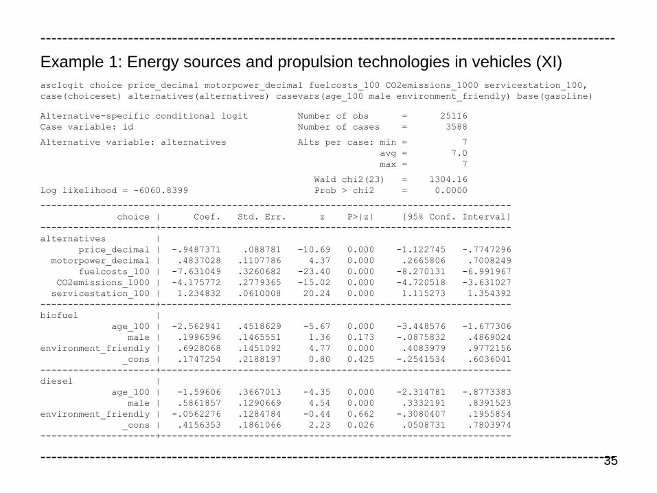
Example 1: Energy sources and propulsion technologies in vehicles (XI)

asclogit choice price_decimal motorpower_decimal fuelcosts_100 CO2emissions_1000 servicestation_100,

case(choiceset) alternatives(alternatives) casevars(age_100 male environment_friendly) base(gasoline)

Alternative-specific conditional logit Number of obs = 25116

Case variable: id Number of cases = 3588

Alternative variable: alternatives Alts per case: min = 7

avg = 7.0

max = 7

Wald chi2(23) = 1304.16

Log likelihood = -6060.8399 Prob > chi2 = 0.0000

--------------------------------------------------------------------------------------

choice | Coef. Std. Err. z P>|z| [95% Conf. Interval]

---------------------+----------------------------------------------------------------

alternatives |

price_decimal | -.9487371 .088781 -10.69 0.000 -1.122745 -.7747296

motorpower_decimal | .4837028 .1107786 4.37 0.000 .2665806 .7008249

fuelcosts_100 | -7.631049 .3260682 -23.40 0.000 -8.270131 -6.991967

CO2emissions_1000 | -4.175772 .2779365 -15.02 0.000 -4.720518 -3.631027

servicestation_100 | 1.234832 .0610008 20.24 0.000 1.115273 1.354392

---------------------+----------------------------------------------------------------

biofuel |

age_100 | -2.562941 .4518629 -5.67 0.000 -3.448576 -1.677306

male | .1996596 .1465551 1.36 0.173 -.0875832 .4869024

environment_friendly | .6928068 .1451092 4.77 0.000 .4083979 .9772156

_cons | .1747254 .2188197 0.80 0.425 -.2541534 .6036041

---------------------+----------------------------------------------------------------

diesel |

age_100 | -1.59606 .3667013 -4.35 0.000 -2.314781 -.8773383

male | .5861857 .1290669 4.54 0.000 .3332191 .8391523

environment_friendly | -.0562276 .1284784 -0.44 0.662 -.3080407 .1955854

_cons | .4156353 .1861066 2.23 0.026 .0508731 .7803974

---------------------+----------------------------------------------------------------

---------------------------------------------------------------------------------------------------------

36

---------------------------------------------------------------------------------------------------------

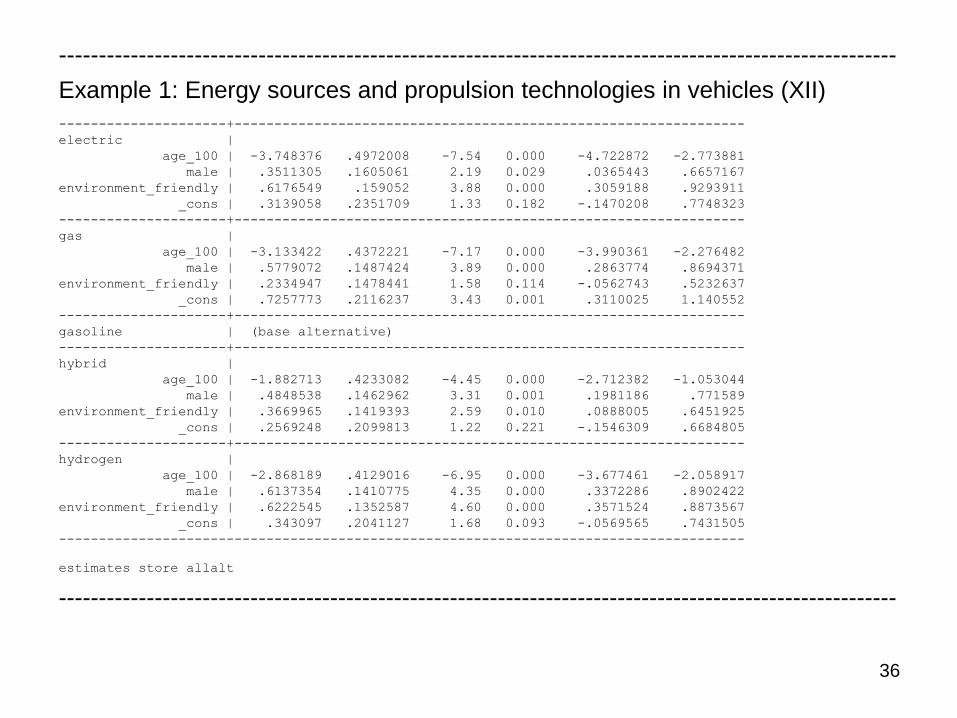
Example 1: Energy sources and propulsion technologies in vehicles (XII)

---------------------+----------------------------------------------------------------

electric |

age_100 | -3.748376 .4972008 -7.54 0.000 -4.722872 -2.773881

male | .3511305 .1605061 2.19 0.029 .0365443 .6657167

environment_friendly | .6176549 .159052 3.88 0.000 .3059188 .9293911

_cons | .3139058 .2351709 1.33 0.182 -.1470208 .7748323

---------------------+----------------------------------------------------------------

gas |

age_100 | -3.133422 .4372221 -7.17 0.000 -3.990361 -2.276482

male | .5779072 .1487424 3.89 0.000 .2863774 .8694371

environment_friendly | .2334947 .1478441 1.58 0.114 -.0562743 .5232637

_cons | .7257773 .2116237 3.43 0.001 .3110025 1.140552

---------------------+----------------------------------------------------------------

gasoline | (base alternative)

---------------------+----------------------------------------------------------------

hybrid |

age_100 | -1.882713 .4233082 -4.45 0.000 -2.712382 -1.053044

male | .4848538 .1462962 3.31 0.001 .1981186 .771589

environment_friendly | .3669965 .1419393 2.59 0.010 .0888005 .6451925

_cons | .2569248 .2099813 1.22 0.221 -.1546309 .6684805

---------------------+----------------------------------------------------------------

hydrogen |

age_100 | -2.868189 .4129016 -6.95 0.000 -3.677461 -2.058917

male | .6137354 .1410775 4.35 0.000 .3372286 .8902422

environment_friendly | .6222545 .1352587 4.60 0.000 .3571524 .8873567

_cons | .343097 .2041127 1.68 0.093 -.0569565 .7431505

--------------------------------------------------------------------------------------

estimates store allalt

---------------------------------------------------------------------------------------------------------

37

---------------------------------------------------------------------------------------------------------

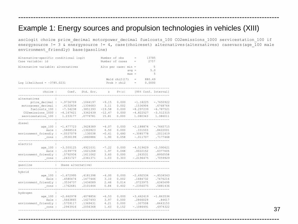
Example 1: Energy sources and propulsion technologies in vehicles (XIII)

asclogit choice price_decimal motorpower_decimal fuelcosts_100 CO2emissions_1000 servicestation_100 if

energysource != 3 & energysource != 4, case(choiceset) alternatives(alternatives) casevars(age_100 male

environment_friendly) base(gasoline)

Alternative-specific conditional logit Number of obs = 13785

Case variable: id Number of cases = 2757

Alternative variable: alternatives Alts per case: min = 5

avg = 5.0

max = 5

Wald chi2(17) = 880.49

Log likelihood = -3785.0231 Prob > chi2 = 0.0000

--------------------------------------------------------------------------------------

choice | Coef. Std. Err. z P>|z| [95% Conf. Interval]

---------------------+----------------------------------------------------------------

alternatives |

price_decimal | -.9736709 .1064197 -9.15 0.000 -1.18225 -.7650922

motorpower_decimal | .4152834 .1334683 3.11 0.002 .1536904 .6768764

fuelcosts_100 | -7.54238 .3851393 -19.58 0.000 -8.297239 -6.787521

CO2emissions_1000 | -4.167421 .3342439 -12.47 0.000 -4.822527 -3.512315

servicestation_100 | 1.233177 .0779781 15.81 0.000 1.080343 1.386011

---------------------+----------------------------------------------------------------

diesel |

age_100 | -1.477723 .3628389 -4.07 0.000 -2.188874 -.7665715

male | .5868516 .1302823 4.50 0.000 .331503 .8422001

environment_friendly | -.0537079 .130038 -0.41 0.680 -.3085778 .2011619

_cons | .3530199 .1860886 1.90 0.058 -.011707 .7177468

---------------------+----------------------------------------------------------------

electric |

age_100 | -3.555125 .4921031 -7.22 0.000 -4.519629 -2.590621

male | .3199779 .1621268 1.97 0.048 .0022152 .6377405

environment_friendly | .5792934 .1611062 3.60 0.000 .263531 .8950558

_cons | .2431727 .2361371 1.03 0.303 -.2196475 .7059929

---------------------+----------------------------------------------------------------

gasoline | (base alternative)

---------------------+----------------------------------------------------------------

hybrid |

age_100 | -1.672995 .4181398 -4.00 0.000 -2.492534 -.8534563

male | .4580474 .1477446 3.10 0.002 .1684732 .7476216

environment_friendly | .3534737 .1434089 2.46 0.014 .0723975 .6345499

_cons | .1762681 .2101444 0.84 0.402 -.2356075 .5881436

---------------------+----------------------------------------------------------------

hydrogen |

age_100 | -2.662978 .4078856 -6.53 0.000 -3.462419 -1.863536

male | .5663865 .1427493 3.97 0.000 .2866029 .84617

environment_friendly | .5759117 .1369431 4.21 0.000 .307508 .8443153

_cons | .2943916 .2056368 1.43 0.152 -.1086491 .6974322

--------------------------------------------------------------------------------------

---------------------------------------------------------------------------------------------------------

38

---------------------------------------------------------------------------------------------------------

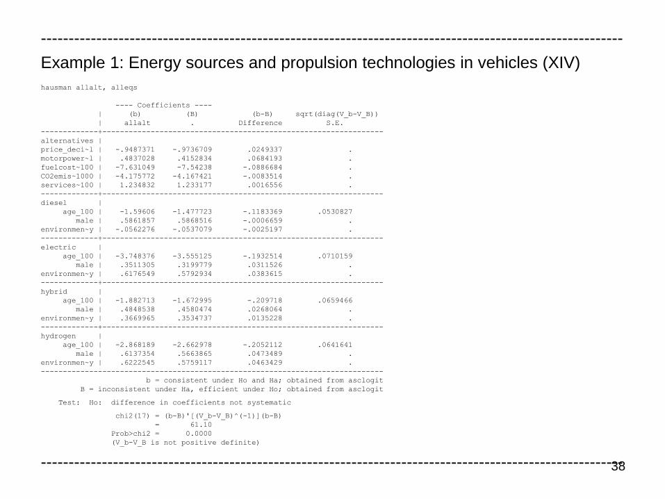
Example 1: Energy sources and propulsion technologies in vehicles (XIV)

hausman allalt, alleqs

---- Coefficients ----

| (b) (B) (b-B) sqrt(diag(V_b-V_B))

| allalt . Difference S.E.

-------------+----------------------------------------------------------------

alternatives |

price_deci~l | -.9487371 -.9736709 .0249337 .

motorpower~l | .4837028 .4152834 .0684193 .

fuelcost~100 | -7.631049 -7.54238 -.0886684 .

CO2emis~1000 | -4.175772 -4.167421 -.0083514 .

services~100 | 1.234832 1.233177 .0016556 .

-------------+----------------------------------------------------------------

diesel |

age_100 | -1.59606 -1.477723 -.1183369 .0530827

male | .5861857 .5868516 -.0006659 .

environmen~y | -.0562276 -.0537079 -.0025197 .

-------------+----------------------------------------------------------------

electric |

age_100 | -3.748376 -3.555125 -.1932514 .0710159

male | .3511305 .3199779 .0311526 .

environmen~y | .6176549 .5792934 .0383615 .

-------------+----------------------------------------------------------------

hybrid |

age_100 | -1.882713 -1.672995 -.209718 .0659466

male | .4848538 .4580474 .0268064 .

environmen~y | .3669965 .3534737 .0135228 .

-------------+----------------------------------------------------------------

hydrogen |

age_100 | -2.868189 -2.662978 -.2052112 .0641641

male | .6137354 .5663865 .0473489 .

environmen~y | .6222545 .5759117 .0463429 .

------------------------------------------------------------------------------

b = consistent under Ho and Ha; obtained from asclogit

B = inconsistent under Ha, efficient under Ho; obtained from asclogit

Test: Ho: difference in coefficients not systematic

chi2(17) = (b-B)'[(V_b-V_B)^(-1)](b-B)

= 61.10

Prob>chi2 = 0.0000

(V_b-V_B is not positive definite)

---------------------------------------------------------------------------------------------------------

39

---------------------------------------------------------------------------------------------------------

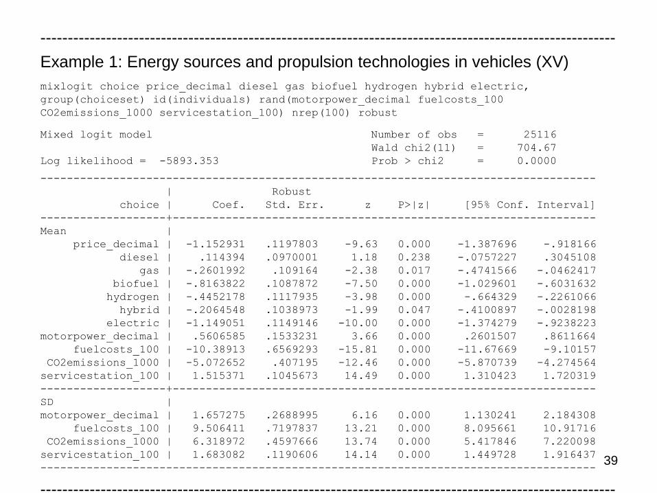
Example 1: Energy sources and propulsion technologies in vehicles (XV)

mixlogit choice price_decimal diesel gas biofuel hydrogen hybrid electric,

group(choiceset) id(individuals) rand(motorpower_decimal fuelcosts_100

CO2emissions_1000 servicestation_100) nrep(100) robust

Mixed logit model Number of obs = 25116

Wald chi2(11) = 704.67

Log likelihood = -5893.353 Prob > chi2 = 0.0000

------------------------------------------------------------------------------------

| Robust

choice | Coef. Std. Err. z P>|z| [95% Conf. Interval]

-------------------+----------------------------------------------------------------

Mean |

price_decimal | -1.152931 .1197803 -9.63 0.000 -1.387696 -.918166

diesel | .114394 .0970001 1.18 0.238 -.0757227 .3045108

gas | -.2601992 .109164 -2.38 0.017 -.4741566 -.0462417

biofuel | -.8163822 .1087872 -7.50 0.000 -1.029601 -.6031632

hydrogen | -.4452178 .1117935 -3.98 0.000 -.664329 -.2261066

hybrid | -.2064548 .1038973 -1.99 0.047 -.4100897 -.0028198

electric | -1.149051 .1149146 -10.00 0.000 -1.374279 -.9238223

motorpower_decimal | .5606585 .1533231 3.66 0.000 .2601507 .8611664

fuelcosts_100 | -10.38913 .6569293 -15.81 0.000 -11.67669 -9.10157

CO2emissions_1000 | -5.072652 .407195 -12.46 0.000 -5.870739 -4.274564

servicestation_100 | 1.515371 .1045673 14.49 0.000 1.310423 1.720319

-------------------+----------------------------------------------------------------

SD |

motorpower_decimal | 1.657275 .2688995 6.16 0.000 1.130241 2.184308

fuelcosts_100 | 9.506411 .7197837 13.21 0.000 8.095661 10.91716

CO2emissions_1000 | 6.318972 .4597666 13.74 0.000 5.417846 7.220098

servicestation_100 | 1.683082 .1190606 14.14 0.000 1.449728 1.916437

------------------------------------------------------------------------------------

---------------------------------------------------------------------------------------------------------

40

---------------------------------------------------------------------------------------------------------

Example 1: Energy sources and propulsion technologies in vehicles (XVI)

mixlogit choice price_decimal diesel gas biofuel hydrogen hybrid electric age_diesel age_gas

age_biofuel age_hydrogen age_hybrid age_electric male_diesel male_gas male_biofuel

male_hydrogen male_hybrid male_electric env_diesel env_gas env_biofuel env_hydrogen env_hybrid

env_electric, group(choiceset) id(individuals) rand(motorpower_decimal fuelcosts_100

CO2emissions_1000 servicestation_100) nrep(5)

Mixed logit model Number of obs = 25116

LR chi2(4) = 252.43

Log likelihood = -5934.6262 Prob > chi2 = 0.0000

------------------------------------------------------------------------------------

choice | Coef. Std. Err. z P>|z| [95% Conf. Interval]

-------------------+----------------------------------------------------------------

Mean |

price_decimal | -1.032654 .0943062 -10.95 0.000 -1.217491 -.847817

diesel | .4778174 .1920106 2.49 0.013 .1014835 .8541512

gas | .861209 .2192962 3.93 0.000 .4313963 1.291022

biofuel | .2782128 .232375 1.20 0.231 -.1772337 .7336594

hydrogen | .3371377 .2186315 1.54 0.123 -.0913721 .7656476

hybrid | .3603566 .2167583 1.66 0.096 -.0644819 .785195

electric | .3766095 .2519047 1.50 0.135 -.1171147 .8703337

age_diesel | -.0174023 .0037944 -4.59 0.000 -.0248391 -.0099655

age_gas | -.0355684 .0045697 -7.78 0.000 -.0445249 -.026612

age_biofuel | -.0305214 .0048031 -6.35 0.000 -.0399353 -.0211076

age_hydrogen | -.0314858 .0044428 -7.09 0.000 -.0401934 -.0227782

age_hybrid | -.0215847 .0043804 -4.93 0.000 -.0301701 -.0129992

age_electric | -.0419787 .005316 -7.90 0.000 -.052398 -.0315595

male_diesel | .6239399 .1338339 4.66 0.000 .3616304 .8862495

male_gas | .622389 .1549903 4.02 0.000 .3186137 .9261644

male_biofuel | .2201399 .1569898 1.40 0.161 -.0875544 .5278342

male_hydrogen | .7132127 .15203 4.69 0.000 .4152394 1.011186

male_hybrid | .5021938 .1522135 3.30 0.001 .2038609 .8005267

male_electric | .3860522 .1712318 2.25 0.024 .0504441 .7216603

---------------------------------------------------------------------------------------------------------

41

---------------------------------------------------------------------------------------------------------

Example 1: Energy sources and propulsion technologies in vehicles (XVII)

-------------------+----------------------------------------------------------------

env_diesel | -.0581815 .1330155 -0.44 0.662 -.3188872 .2025241

env_gas | .2444517 .1536347 1.59 0.112 -.0566668 .5455703

env_biofuel | .7172262 .1547238 4.64 0.000 .4139732 1.020479

env_hydrogen | .6128832 .1460365 4.20 0.000 .3266569 .8991096

env_hybrid | .3709122 .1474779 2.52 0.012 .0818609 .6599636

env_electric | .6119939 .1695082 3.61 0.000 .2797639 .9442239

motorpower_decimal | .5443154 .1178504 4.62 0.000 .3133329 .7752978

fuelcosts_100 | -8.656736 .4241358 -20.41 0.000 -9.488026 -7.825445

CO2emissions_1000 | -4.697025 .3377086 -13.91 0.000 -5.358922 -4.035129

servicestation_100 | 1.316358 .0745108 17.67 0.000 1.170319 1.462396

-------------------+----------------------------------------------------------------

SD |

motorpower_decimal | .0233069 .3343648 0.07 0.944 -.6320361 .6786499

fuelcosts_100 | -6.080686 .6500041 -9.35 0.000 -7.354671 -4.806702

CO2emissions_1000 | 4.922441 .4547904 10.82 0.000 4.031068 5.813814

servicestation_100 | 1.158471 .1103848 10.49 0.000 .942121 1.374821

------------------------------------------------------------------------------------

estimates store mixlogit

asclogit choice price_decimal motorpower_decimal fuelcosts_100 CO2emissions_1000

servicestation_100, case(choiceset) alternatives(alternatives) casevars(age_100 male

environment_friendly) base(gasoline)

lrtest mixlogit, force

Likelihood-ratio test LR chi2(4) = 252.43

(Assumption: . nested in mixlogit) Prob > chi2 = 0.0000

---------------------------------------------------------------------------------------------------------

42

---------------------------------------------------------------------------------------------------------

Example 1: Energy sources and propulsion technologies in vehicles (XVIII)

Estimated WTP (based on the customized purchase price in decimals) for re-

duced CO2 emissions (in 1000 gram per kilometer) and for service station avai-

lability (in decimals of stations with respective fuel):

• Page 32: Multinomial logit model with only alternative specific attributes

- WT PCO2 = -4.325, i.e. the estimated average WTP is approximately

0.4325% of the purchase price for a reduction of the CO2 emissions by 1

gram (which is 0.004325·20725 = 89.64 Euro due to the average pur-

chase price of 20725 Euro)

- WT Pstation = 1.286, i.e. the estimated average WTP is approximately

1.286% of the purchase price for an increase of the service station availa-

bility by 1 percentage point (which is 0.01286·20725 = 266.47 Euro)

• Page 33: Independent multinomial probit model with only alternative specific

attributes

- WT PCO2 = -4.299, i.e. 0.4299% or 0.004299·20725 = 89.09 Euro

- WT Pstation = 1.326, i.e. 1.326% or 0.01326·20725 = 274.71 Euro

---------------------------------------------------------------------------------------------------------

43

---------------------------------------------------------------------------------------------------------

Example 1: Energy sources and propulsion technologies in vehicles (XIX)

• Page 35: Full multinomial logit model

- WT PCO2 = -4.401, i.e. 0.4401% or 0.004401·20725 = 91.22 Euro

- WT Pstation = 1.302, i.e. 1.302% or 0.01302·20725 = 269.75 Euro

• Page 39/40: Mixed logit models with only alternative specific attributes and

full mixed logit model

- WT PCO2 = -4.400 (91.19 Euro) and WT PCO2 = -4.548 (94.27 Euro)

- WT Pstation = 1.314 (272.40 Euro) and 1.1275 (264.19 Euro)

Estimated WTP (based on the purchase price divided by 100000) for reduced

CO2 emissions (in 1000 gram per kilometer) and for service station availability

(in decimals of stations with respective fuel):

• Page 34: Multinomial logit model with only alternative specific attributes

- WT PCO2 = -1.155, i.e. the estimated average WTP is approximately 115,5

Euro for a reduction of the CO2 emissions by 1 gram

- WT Pstation = 0.346, i.e. the estimated average WTP is approximately 346

Euro for an increase of the service station availability by 1 percentage

point

---------------------------------------------------------------------------------------------------------

44

---------------------------------------------------------------------------------------------------------

Example 2: Choice among fixed-interest investment products (I)

In Gutsche and Ziegler (2016), two unlabeled SCE (based on “Balanced Over-

lap” designs for which 50 different versions of randomized choice sets were

created for each SCE and assigned to the respondents) are examined, which

comprised choices among several investment products:

• While one SCE referred to the choice among four different equity funds (the

data are discussed and examined in the tutorial), the other SCE referred to

the choice among four alternative fixed-interest investment products with an

investment horizon of three years

• All data stem from a computer-based survey during December 2013 and Ja-

nuary 2014, carried out in cooperation with the German market research in-

stitute GfK SE, which drew a sample from its internal representative (in

terms of age, gender, and place of origin) online panel

• 1001 respondents from the population of financial decision makers in Ger-

many with a minimum of investment experiences (i.e. the respondents must

have at least a savings account) participated in the survey and thus in this

SCE

• The SCE was based on six choice sets and comprised four attributes, i.e.

provider, yearly nominal interest rate, sustainability criteria, and transpare-

ncy logo

---------------------------------------------------------------------------------------------------------

45

---------------------------------------------------------------------------------------------------------

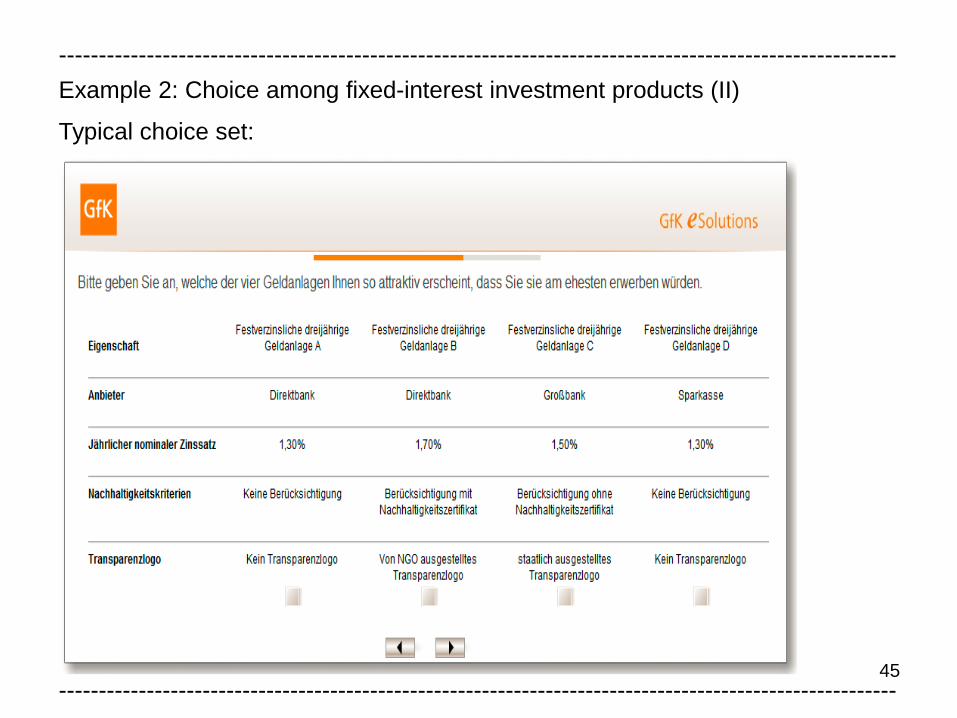
Example 2: Choice among fixed-interest investment products (II)

Typical choice set:

---------------------------------------------------------------------------------------------------------

46

---------------------------------------------------------------------------------------------------------

Example 2: Choice among fixed-interest investment products (III)

Attribute levels:

• Provider (dummy variables): Big bank (base variable), municipal savings

bank, co-operative bank, direct bank, sustainability bank

• Yearly nominal interest rate: 1.30%, 1.50%, 1.70%, 1.90%, 2.10%

• Sustainability criteria (dummy variables): No consideration (base variable),

consideration without sustainability certificate, consideration with sustain-

ability certificate

• Transparency logo (dummy variables): No transparency logo (base variab-

le), transparency logo issued by an NGO, transparency logo issued by the

state

Individual characteristics:

• Social values and norms (dummy variables): Warm glow, expectations from

the social environ-ment, membership to an environmental organization,

affinity with left or right-wings parties

• Socio-demographic variables (dummy variables with the exception of age,

which is measured in years): Female, high education, living together or mar-

ried, Western Germany

---------------------------------------------------------------------------------------------------------

47

---------------------------------------------------------------------------------------------------------

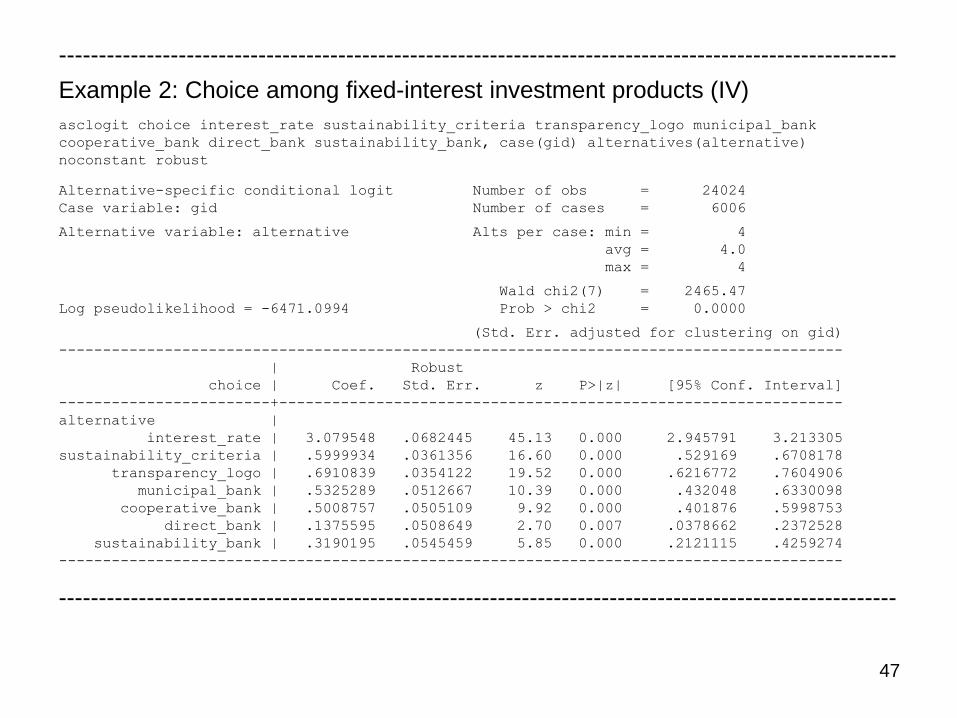
Example 2: Choice among fixed-interest investment products (IV)

asclogit choice interest_rate sustainability_criteria transparency_logo municipal_bank

cooperative_bank direct_bank sustainability_bank, case(gid) alternatives(alternative)

noconstant robust

Alternative-specific conditional logit Number of obs = 24024

Case variable: gid Number of cases = 6006

Alternative variable: alternative Alts per case: min = 4

avg = 4.0

max = 4

Wald chi2(7) = 2465.47

Log pseudolikelihood = -6471.0994 Prob > chi2 = 0.0000

(Std. Err. adjusted for clustering on gid)

-----------------------------------------------------------------------------------------

| Robust

choice | Coef. Std. Err. z P>|z| [95% Conf. Interval]

------------------------+----------------------------------------------------------------

alternative |

interest_rate | 3.079548 .0682445 45.13 0.000 2.945791 3.213305

sustainability_criteria | .5999934 .0361356 16.60 0.000 .529169 .6708178

transparency_logo | .6910839 .0354122 19.52 0.000 .6216772 .7604906

municipal_bank | .5325289 .0512667 10.39 0.000 .432048 .6330098

cooperative_bank | .5008757 .0505109 9.92 0.000 .401876 .5998753

direct_bank | .1375595 .0508649 2.70 0.007 .0378662 .2372528

sustainability_bank | .3190195 .0545459 5.85 0.000 .2121115 .4259274

-----------------------------------------------------------------------------------------

---------------------------------------------------------------------------------------------------------

48

---------------------------------------------------------------------------------------------------------

Example 2: Choice among fixed-interest investment products (V)

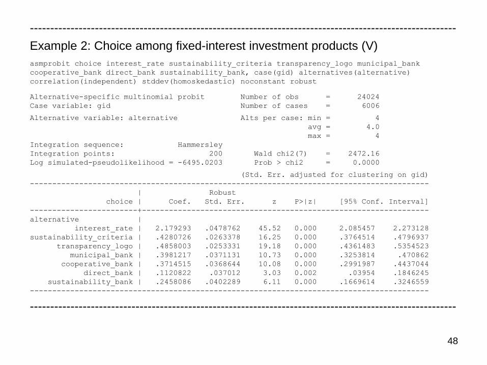
asmprobit choice interest_rate sustainability_criteria transparency_logo municipal_bank

cooperative_bank direct_bank sustainability_bank, case(gid) alternatives(alternative)

correlation(independent) stddev(homoskedastic) noconstant robust

Alternative-specific multinomial probit Number of obs = 24024

Case variable: gid Number of cases = 6006

Alternative variable: alternative Alts per case: min = 4

avg = 4.0

max = 4

Integration sequence: Hammersley

Integration points: 200 Wald chi2(7) = 2472.16

Log simulated-pseudolikelihood = -6495.0203 Prob > chi2 = 0.0000

(Std. Err. adjusted for clustering on gid)

-----------------------------------------------------------------------------------------

| Robust

choice | Coef. Std. Err. z P>|z| [95% Conf. Interval]

------------------------+----------------------------------------------------------------

alternative |

interest_rate | 2.179293 .0478762 45.52 0.000 2.085457 2.273128

sustainability_criteria | .4280726 .0263378 16.25 0.000 .3764514 .4796937

transparency_logo | .4858003 .0253331 19.18 0.000 .4361483 .5354523

municipal_bank | .3981217 .0371131 10.73 0.000 .3253814 .470862

cooperative_bank | .3714515 .0368644 10.08 0.000 .2991987 .4437044

direct_bank | .1120822 .037012 3.03 0.002 .03954 .1846245

sustainability_bank | .2458086 .0402289 6.11 0.000 .1669614 .3246559

-----------------------------------------------------------------------------------------

---------------------------------------------------------------------------------------------------------

49

---------------------------------------------------------------------------------------------------------

Example 2: Choice among fixed-interest investment products (VI)

mixlogit choice interest_rate, group(gid) id(id) rand(sustainability_criteria transparency_logo

municipal_bank cooperative_bank direct_bank sustainability_bank) nrep(10)

Mixed logit model Number of obs = 24024

LR chi2(6) = 409.16

Log likelihood = -6266.5199 Prob > chi2 = 0.0000

-----------------------------------------------------------------------------------------

choice | Coef. Std. Err. z P>|z| [95% Conf. Interval]

------------------------+----------------------------------------------------------------

Mean |

interest_rate | 3.535709 .0778741 45.40 0.000 3.383079 3.68834

sustainability_criteria | .7223758 .0481924 14.99 0.000 .6279205 .816831

transparency_logo | .8350265 .0467344 17.87 0.000 .7434288 .9266242

municipal_bank | .5144328 .0654726 7.86 0.000 .3861088 .6427568

cooperative_bank | .5070607 .0614912 8.25 0.000 .3865402 .6275812

direct_bank | .1352623 .0575323 2.35 0.019 .022501 .2480236

sustainability_bank | .251023 .0649031 3.87 0.000 .1238151 .3782308

------------------------+----------------------------------------------------------------

SD |

sustainability_criteria | .8885514 .0662333 13.42 0.000 .7587366 1.018366

transparency_logo | .6820224 .0844074 8.08 0.000 .5165869 .847458

municipal_bank | 1.057992 .0860352 12.30 0.000 .8893658 1.226618

cooperative_bank | .692157 .0867893 7.98 0.000 .522053 .862261

direct_bank | -.1793131 .097308 -1.84 0.065 -.3700332 .0114071

sustainability_bank | -.7008728 .1002378 -6.99 0.000 -.8973352 -.5044104

-----------------------------------------------------------------------------------------

estimates store fullmixedlogit

---------------------------------------------------------------------------------------------------------

50

---------------------------------------------------------------------------------------------------------

Example 2: Choice among fixed-interest investment products (VII)

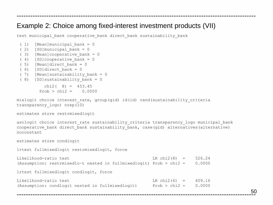
test municipal_bank cooperative_bank direct_bank sustainability_bank

( 1) [Mean]municipal_bank = 0

( 2) [SD]municipal_bank = 0

( 3) [Mean]cooperative_bank = 0

( 4) [SD]cooperative_bank = 0

( 5) [Mean]direct_bank = 0

( 6) [SD]direct_bank = 0

( 7) [Mean]sustainability_bank = 0

( 8) [SD]sustainability_bank = 0

chi2( 8) = 453.45

Prob > chi2 = 0.0000

mixlogit choice interest_rate, group(gid) id(id) rand(sustainability_criteria

transparency_logo) nrep(10)

estimates store restrmixedlogit

asclogit choice interest_rate sustainability_criteria transparency_logo municipal_bank

cooperative_bank direct_bank sustainability_bank, case(gid) alternatives(alternative)

noconstant

estimates store condlogit

lrtest fullmixedlogit restrmixedlogit, force

Likelihood-ratio test LR chi2(8) = 326.24

(Assumption: restrmixedlo~t nested in fullmixedlogit) Prob > chi2 = 0.0000

lrtest fullmixedlogit condlogit, force

Likelihood-ratio test LR chi2(6) = 409.16

(Assumption: condlogit nested in fullmixedlogit) Prob > chi2 = 0.0000

---------------------------------------------------------------------------------------------------------

51

---------------------------------------------------------------------------------------------------------

Example 2: Choice among fixed-interest investment products (VIII)

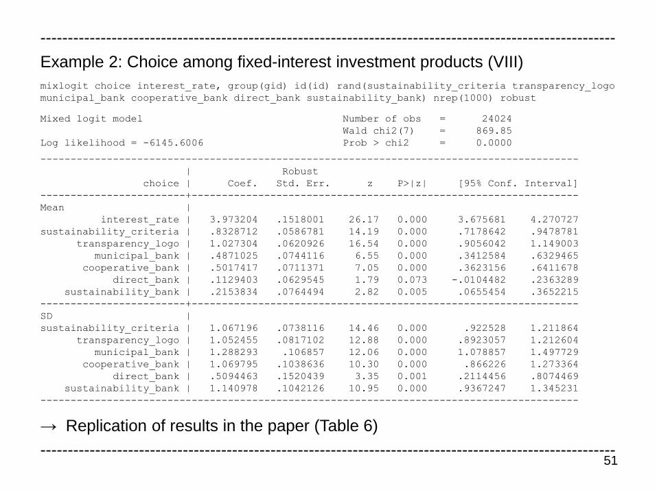
mixlogit choice interest_rate, group(gid) id(id) rand(sustainability_criteria transparency_logo

municipal_bank cooperative_bank direct_bank sustainability_bank) nrep(1000) robust

Mixed logit model Number of obs = 24024

Wald chi2(7) = 869.85

Log likelihood = -6145.6006 Prob > chi2 = 0.0000

-----------------------------------------------------------------------------------------

| Robust

choice | Coef. Std. Err. z P>|z| [95% Conf. Interval]

------------------------+----------------------------------------------------------------

Mean |

interest_rate | 3.973204 .1518001 26.17 0.000 3.675681 4.270727

sustainability_criteria | .8328712 .0586781 14.19 0.000 .7178642 .9478781

transparency_logo | 1.027304 .0620926 16.54 0.000 .9056042 1.149003

municipal_bank | .4871025 .0744116 6.55 0.000 .3412584 .6329465

cooperative_bank | .5017417 .0711371 7.05 0.000 .3623156 .6411678

direct_bank | .1129403 .0629545 1.79 0.073 -.0104482 .2363289

sustainability_bank | .2153834 .0764494 2.82 0.005 .0655454 .3652215

------------------------+----------------------------------------------------------------

SD |

sustainability_criteria | 1.067196 .0738116 14.46 0.000 .922528 1.211864

transparency_logo | 1.052455 .0817102 12.88 0.000 .8923057 1.212604

municipal_bank | 1.288293 .106857 12.06 0.000 1.078857 1.497729

cooperative_bank | 1.069795 .1038636 10.30 0.000 .866226 1.273364

direct_bank | .5094463 .1520439 3.35 0.001 .2114456 .8074469

sustainability_bank | 1.140978 .1042126 10.95 0.000 .9367247 1.345231

-----------------------------------------------------------------------------------------

→ Replication of results in the paper (Table 6)

---------------------------------------------------------------------------------------------------------

52

---------------------------------------------------------------------------------------------------------

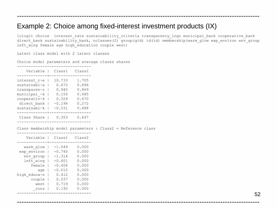
Example 2: Choice among fixed-interest investment products (IX)

lclogit choice interest_rate sustainability_criteria transparency_logo municipal_bank cooperative_bank

direct_bank sustainability_bank, nclasses(2) group(gid) id(id) membership(warm_glow exp_environ env_group

left_wing female age high_education couple west)

Latent class model with 2 latent classes

Choice model parameters and average classs shares

--------------------------------

Variable | Class1 Class2

-------------+------------------

interest_r~e | 10.733 1.705

sustainabi~a | 0.672 0.896

transparen~o | 0.945 0.869

municipal_~k | 0.150 0.685

cooperativ~k | 0.329 0.670

direct_bank | -0.196 0.272

sustainabi~k | -0.531 0.488

-------------+------------------

Class Share | 0.353 0.647

--------------------------------

Class membership model parameters : Class2 = Reference class

--------------------------------

Variable | Class1 Class2

-------------+------------------

warm_glow | -1.049 0.000

exp_environ | -0.740 0.000

env_group | -1.314 0.000

left_wing | -0.601 0.000

female | -0.406 0.000

age | -0.015 0.000

high_educa~n | 0.412 0.000

couple | 0.037 0.000

west | 0.719 0.000

_cons | 0.192 0.000

--------------------------------

---------------------------------------------------------------------------------------------------------

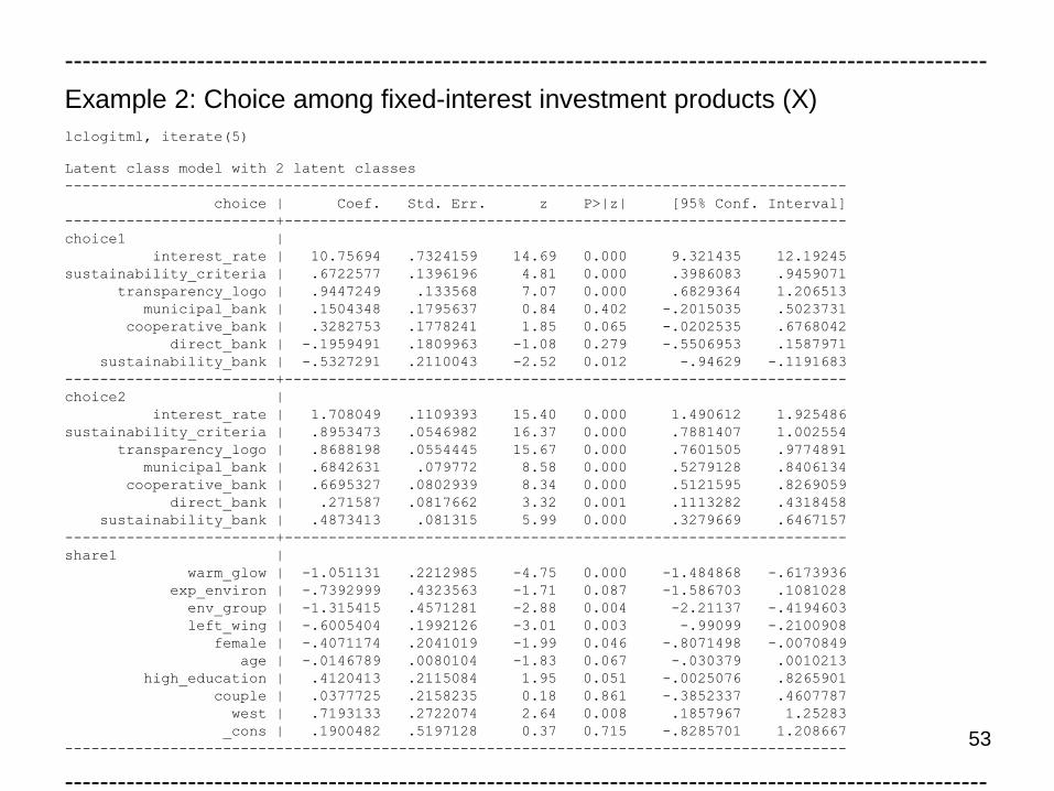
53

---------------------------------------------------------------------------------------------------------

Example 2: Choice among fixed-interest investment products (X)

lclogitml, iterate(5)

Latent class model with 2 latent classes

-----------------------------------------------------------------------------------------

choice | Coef. Std. Err. z P>|z| [95% Conf. Interval]

------------------------+----------------------------------------------------------------

choice1 |

interest_rate | 10.75694 .7324159 14.69 0.000 9.321435 12.19245

sustainability_criteria | .6722577 .1396196 4.81 0.000 .3986083 .9459071

transparency_logo | .9447249 .133568 7.07 0.000 .6829364 1.206513

municipal_bank | .1504348 .1795637 0.84 0.402 -.2015035 .5023731

cooperative_bank | .3282753 .1778241 1.85 0.065 -.0202535 .6768042

direct_bank | -.1959491 .1809963 -1.08 0.279 -.5506953 .1587971

sustainability_bank | -.5327291 .2110043 -2.52 0.012 -.94629 -.1191683

------------------------+----------------------------------------------------------------

choice2 |

interest_rate | 1.708049 .1109393 15.40 0.000 1.490612 1.925486

sustainability_criteria | .8953473 .0546982 16.37 0.000 .7881407 1.002554

transparency_logo | .8688198 .0554445 15.67 0.000 .7601505 .9774891

municipal_bank | .6842631 .079772 8.58 0.000 .5279128 .8406134

cooperative_bank | .6695327 .0802939 8.34 0.000 .5121595 .8269059

direct_bank | .271587 .0817662 3.32 0.001 .1113282 .4318458

sustainability_bank | .4873413 .081315 5.99 0.000 .3279669 .6467157

------------------------+----------------------------------------------------------------

share1 |

warm_glow | -1.051131 .2212985 -4.75 0.000 -1.484868 -.6173936

exp_environ | -.7392999 .4323563 -1.71 0.087 -1.586703 .1081028

env_group | -1.315415 .4571281 -2.88 0.004 -2.21137 -.4194603

left_wing | -.6005404 .1992126 -3.01 0.003 -.99099 -.2100908

female | -.4071174 .2041019 -1.99 0.046 -.8071498 -.0070849

age | -.0146789 .0080104 -1.83 0.067 -.030379 .0010213

high_education | .4120413 .2115084 1.95 0.051 -.0025076 .8265901

couple | .0377725 .2158235 0.18 0.861 -.3852337 .4607787

west | .7193133 .2722074 2.64 0.008 .1857967 1.25283

_cons | .1900482 .5197128 0.37 0.715 -.8285701 1.208667

-----------------------------------------------------------------------------------------

---------------------------------------------------------------------------------------------------------

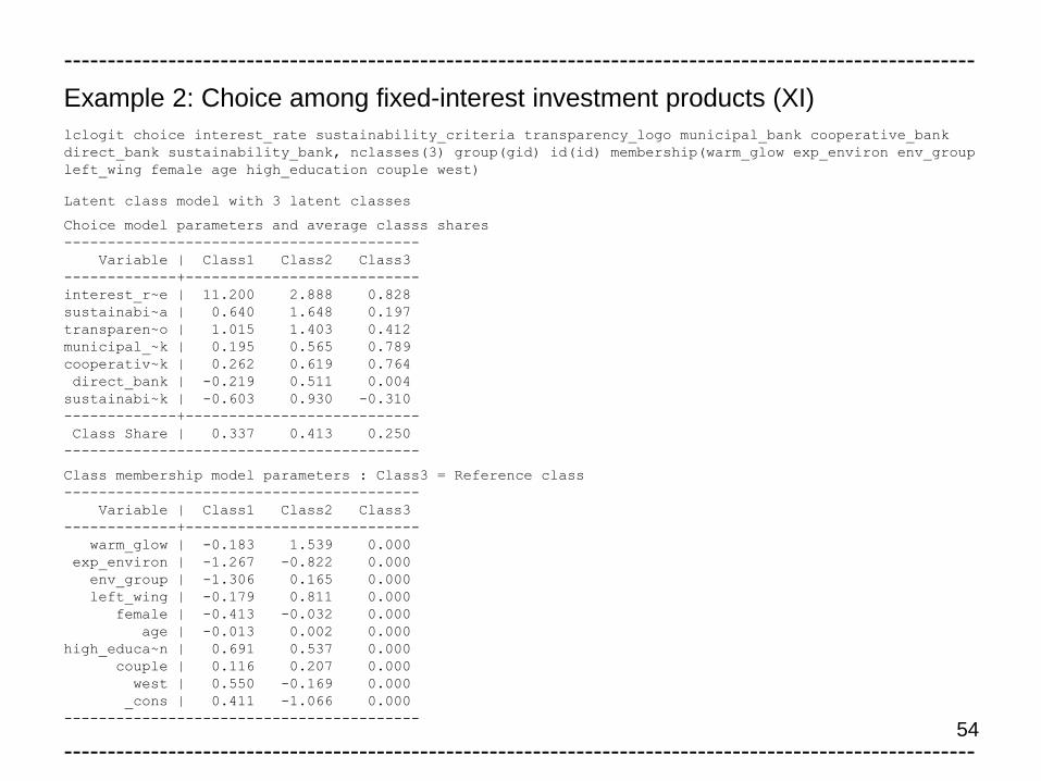
54

---------------------------------------------------------------------------------------------------------

Example 2: Choice among fixed-interest investment products (XI)

lclogit choice interest_rate sustainability_criteria transparency_logo municipal_bank cooperative_bank

direct_bank sustainability_bank, nclasses(3) group(gid) id(id) membership(warm_glow exp_environ env_group

left_wing female age high_education couple west)

Latent class model with 3 latent classes

Choice model parameters and average classs shares

-----------------------------------------

Variable | Class1 Class2 Class3

-------------+---------------------------

interest_r~e | 11.200 2.888 0.828

sustainabi~a | 0.640 1.648 0.197

transparen~o | 1.015 1.403 0.412

municipal_~k | 0.195 0.565 0.789

cooperativ~k | 0.262 0.619 0.764

direct_bank | -0.219 0.511 0.004

sustainabi~k | -0.603 0.930 -0.310

-------------+---------------------------

Class Share | 0.337 0.413 0.250

-----------------------------------------

Class membership model parameters : Class3 = Reference class

-----------------------------------------

Variable | Class1 Class2 Class3

-------------+---------------------------

warm_glow | -0.183 1.539 0.000

exp_environ | -1.267 -0.822 0.000

env_group | -1.306 0.165 0.000

left_wing | -0.179 0.811 0.000

female | -0.413 -0.032 0.000

age | -0.013 0.002 0.000

high_educa~n | 0.691 0.537 0.000

couple | 0.116 0.207 0.000

west | 0.550 -0.169 0.000

_cons | 0.411 -1.066 0.000

-----------------------------------------

---------------------------------------------------------------------------------------------------------

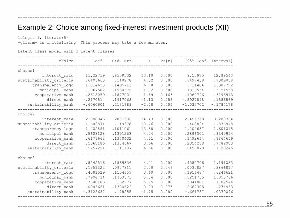
55

---------------------------------------------------------------------------------------------------------

Example 2: Choice among fixed-interest investment products (XII)

lclogitml, iterate(5)

-gllamm- is initializing. This process may take a few minutes.

Latent class model with 3 latent classes

-----------------------------------------------------------------------------------------

choice | Coef. Std. Err. z P>|z| [95% Conf. Interval]

------------------------+----------------------------------------------------------------

choice1 |

interest_rate | 11.22759 .8509532 13.19 0.000 9.55975 12.89543

sustainability_criteria | .6403663 .148278 4.32 0.000 .3497468 .9309858

transparency_logo | 1.014638 .1495712 6.78 0.000 .721484 1.307792

municipal_bank | .1967502 .1930676 1.02 0.308 -.1816554 .5751558

cooperative_bank | .2618059 .1877001 1.39 0.163 -.1060796 .6296913

direct_bank | -.2170514 .1917068 -1.13 0.258 -.5927898 .1586869

sustainability_bank | -.6060601 .2181889 -2.78 0.005 -1.033702 -.1784178

------------------------+----------------------------------------------------------------

choice2 |

interest_rate | 2.888046 .2001506 14.43 0.000 2.495758 3.280334

sustainability_criteria | 1.642871 .119378 13.76 0.000 1.408894 1.876848

transparency_logo | 1.402851 .1011061 13.88 0.000 1.204687 1.601015

municipal_bank | .5623128 .1391263 4.04 0.000 .2896302 .8349954

cooperative_bank | .6178662 .1370432 4.51 0.000 .3492664 .8864659

direct_bank | .5068186 .1384667 3.66 0.000 .2354288 .7782083

sustainability_bank | .9257291 .141187 6.56 0.000 .6490078 1.20245

------------------------+----------------------------------------------------------------

choice3 |

interest_rate | .8245516 .1869836 4.41 0.000 .4580706 1.191033

sustainability_criteria | .1951322 .0977311 2.00 0.046 .0035827 .3866817

transparency_logo | .4081529 .1104659 3.69 0.000 .1916437 .6246621

municipal_bank | .7904714 .1353571 5.84 0.000 .5251765 1.055766

cooperative_bank | .7648103 .132977 5.75 0.000 .5041801 1.02544

direct_bank | .0043661 .1380622 0.03 0.975 -.2662308 .274963

sustainability_bank | -.3123637 .178255 -1.75 0.080 -.661737 .0370096

------------------------+----------------------------------------------------------------

---------------------------------------------------------------------------------------------------------

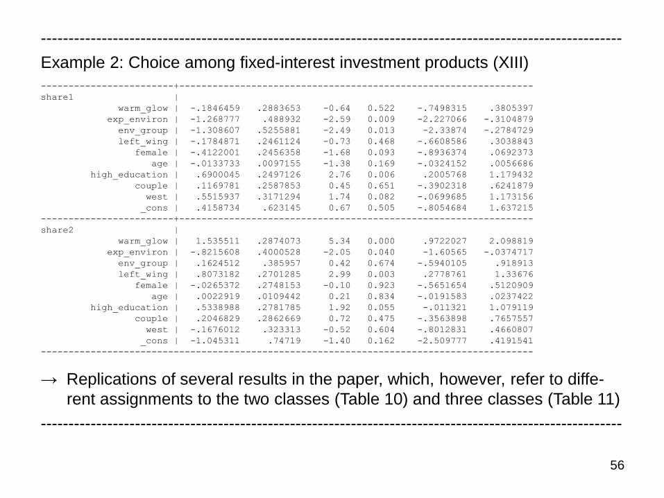
56

---------------------------------------------------------------------------------------------------------

Example 2: Choice among fixed-interest investment products (XIII)

------------------------+----------------------------------------------------------------

share1 |

warm_glow | -.1846459 .2883653 -0.64 0.522 -.7498315 .3805397

exp_environ | -1.268777 .488932 -2.59 0.009 -2.227066 -.3104879

env_group | -1.308607 .5255881 -2.49 0.013 -2.33874 -.2784729

left_wing | -.1784871 .2461124 -0.73 0.468 -.6608586 .3038843

female | -.4122001 .2456358 -1.68 0.093 -.8936374 .0692373

age | -.0133733 .0097155 -1.38 0.169 -.0324152 .0056686

high_education | .6900045 .2497126 2.76 0.006 .2005768 1.179432

couple | .1169781 .2587853 0.45 0.651 -.3902318 .6241879

west | .5515937 .3171294 1.74 0.082 -.0699685 1.173156

_cons | .4158734 .623145 0.67 0.505 -.8054684 1.637215

------------------------+----------------------------------------------------------------

share2 |

warm_glow | 1.535511 .2874073 5.34 0.000 .9722027 2.098819

exp_environ | -.8215608 .4000528 -2.05 0.040 -1.60565 -.0374717

env_group | .1624512 .385957 0.42 0.674 -.5940105 .918913

left_wing | .8073182 .2701285 2.99 0.003 .2778761 1.33676

female | -.0265372 .2748153 -0.10 0.923 -.5651654 .5120909

age | .0022919 .0109442 0.21 0.834 -.0191583 .0237422

high_education | .5338988 .2781785 1.92 0.055 -.011321 1.079119

couple | .2046829 .2862669 0.72 0.475 -.3563898 .7657557

west | -.1676012 .323313 -0.52 0.604 -.8012831 .4660807

_cons | -1.045311 .74719 -1.40 0.162 -2.509777 .4191541

-----------------------------------------------------------------------------------------

→ Replications of several results in the paper, which, however, refer to diffe-

rent assignments to the two classes (Table 10) and three classes (Table 11)

---------------------------------------------------------------------------------------------------------