3. Linear Least Squares Problems

Linear Least Squares Problems

3.1. Introduction

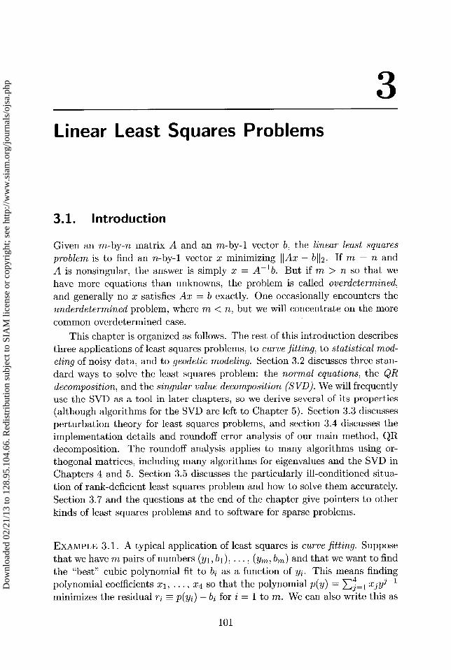
Given an m-by-n matrix A and an m-by-1 vector b, the linear least squaresproblem is to find an n-by-1 vector x minimizing Ax — bil2. If m = n and

A is nonsingular, the answer is simply x = A—l b. But if m > n so that we

have more equations than unknowns, the problem is called overdetermined,and generally no x satisfies Ax = b exactly. One occasionally encounters the

underdetermined problem, where m < n, but we will concentrate on the more

common overdetermined case.

This chapter is organized as follows. The rest of this introduction describesthree applications of least squares problems, to curve fitting, to statistical rnod-eling of noisy data, and to geodetic modeling. Section 3.2 discusses three stan-

dard ways to solve the least squares problem: the normal equations, the QRdecomposition, and the singular value decomposition (SVD). We will frequentlyuse the SVD as a tool in later chapters, so we derive several of its properties(although algorithms for the SVD are left to Chapter 5). Section 3.3 discussesperturbation theory for least squares problems, and section 3.4 discusses theimplementation details and roundoff error analysis of our main method, QRdecomposition. The roundoff analysis applies to many algorithms using or-thogonal matrices, including many algorithms for eigenvalues and the SVD inChapters 4 and 5. Section 3.5 discusses the particularly ill-conditioned situa-

tion of rank-deficient least squares problem and how to solve them accurately.Section 3.7 and the questions at the end of the chapter give pointers to other

kinds of least squares problems and to software for sparse problems.

EXAMPLE 3.1. A typical application of least squares is curve fitting. Suppose

that we have m pairs of numbers (yl, bi), ... , (yr,,,, bm ) and that we want to find

the "best" cubic polynomial fit to bi as a function of yz. This means finding

polynomial coefficients xl, ... , x4 so that the polynomial p(y) _ >j xjy^-1minimizes the residual ri - p(y2) — bi for i = 1 to m. We can also write this as

101

Dow

nloa

ded

02/2

1/13

to 1

28.9

5.10

4.66

. Red

istr

ibut

ion

subj

ect t

o SI

AM

lice

nse

or c

opyr

ight

; see

http

://w

ww

.sia

m.o

rg/jo

urna

ls/o

jsa.

php

102 Applied Numerical Linear Algebra

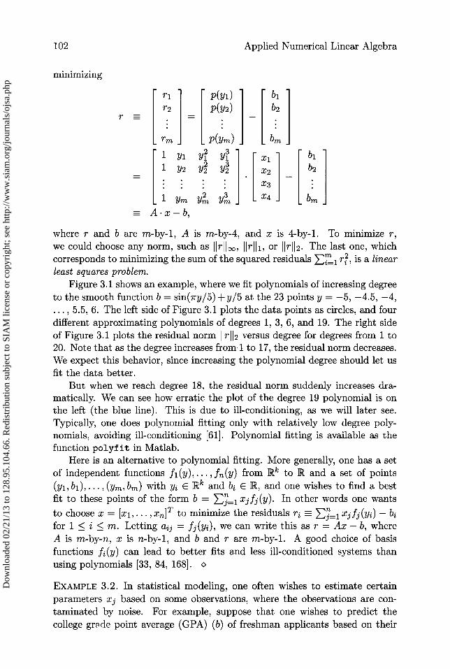
minimizing

r1 p(yi) bi

r2 p(y2) b2r - _ —rm P(ym) bm

1 yl yi yi xl bl1 Y2 Y2 Y2 x2 b2

X3

1 ym ym ymX4 bm

A•x—b,

where r and b are m-by-1, A is m-by-4, and x is 4-by-1. To minimize r,we could choose any norm, such as IIrI, IIrIi, or 1r 2. The last one, whichcorresponds to minimizing the sum of the squared residuals ^m r2, is a linearleast squares problem.

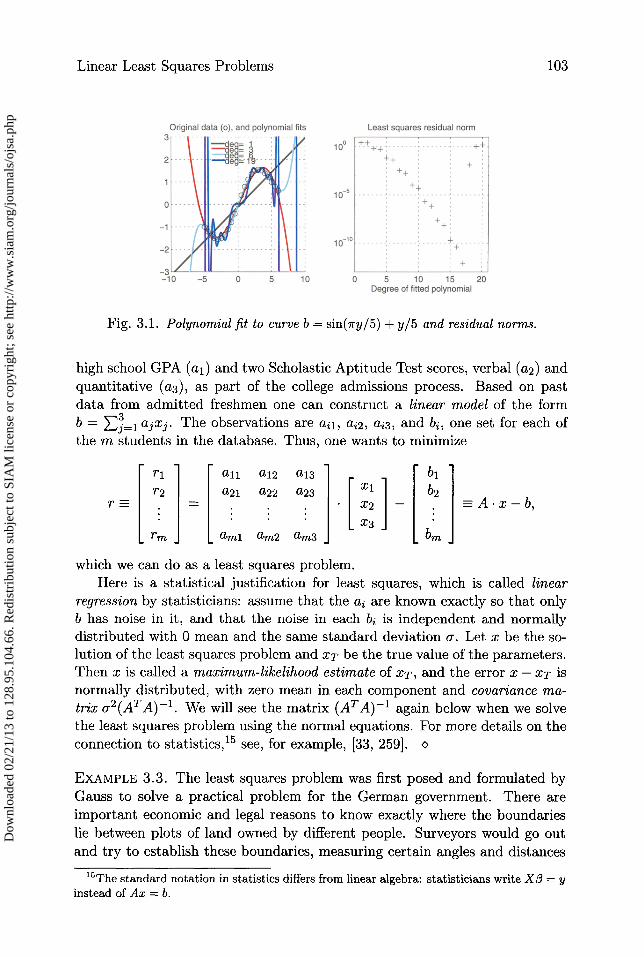
Figure 3.1 shows an example, where we fit polynomials of increasing degreeto the smooth function b = sin(iry/5) + y/5 at the 23 points y = —5, —4.5, —4,... , 5.5, 6. The left side of Figure 3.1 plots the data points as circles, and fourdifferent approximating polynomials of degrees 1, 3, 6, and 19. The right sideof Figure 3.1 plots the residual norm r 112 versus degree for degrees from 1 to20. Note that as the degree increases from 1 to 17, the residual norm decreases.We expect this behavior, since increasing the polynomial degree should let usfit the data better.

But when we reach degree 18, the residual norm suddenly increases dra-matically. We can see how erratic the plot of the degree 19 polynomial is onthe left (the blue line). This is due to ill-conditioning, as we will later see.Typically, one does polynomial fitting only with relatively low degree poly-nomials, avoiding ill-conditioning [61]. Polynomial fitting is available as thefunction polyf it in Matlab.

Here is an alternative to polynomial fitting. More generally, one has a setof independent functions fl (y), ... , f(y) from I[8k to I[8 and a set of points

(yl, bi), ... , (ym, bm ) with y2 E Rk and bi E R, and one wishes to find a bestfit to these points of the form b = E^ 1 x^ f^(y). In other words one wants

to choose x = [xl, ... , xn ] T to minimize the residuals ri = E^ 1 x3 f^ (yz) — bifor 1 < i < m. Letting = f^(y2), we can write this as r = Ax — b, whereA is m-by-n, x is n-by-1, and b and r are m-by-1. A good choice of basisfunctions f(y) can lead to better fits and less ill-conditioned systems thanusing polynomials [33, 84, 168]. o

EXAMPLE 3.2. In statistical modeling, one often wishes to estimate certainparameters xj based on some observations, where the observations are con-taminated by noise. For example, suppose that one wishes to predict thecollege grade point average (GPA) (b) of freshman applicants based on their

Dow

nloa

ded

02/2

1/13

to 1

28.9

5.10

4.66

. Red

istr

ibut

ion

subj

ect t

o SI

AM

lice

nse

or c

opyr

ight

; see

http

://w

ww

.sia

m.o

rg/jo

urna

ls/o

jsa.

php


103

Fig. 3.1. Polynomial fit to curve b = sin(7ry/5) + y/5 and residual norms.

high school GPA (a1) and two Scholastic Aptitude Test scores, verbal (a2) andquantitative (a3), as part of the college admissions process. Based on pastdata from admitted freshmen one can construct a linear model of the formb = E^__ 1 a^x^. The observations are ai1, ai2, az3, and bi, one set for each ofthe m students in the database. Thus, one wants to minimize

r1 all a12 a13 b1

r2 a21 a22 a23 x1 b2r- = X2 — -A•x—b,

X3

rm aml am2 am3 bm

which we can do as a least squares problem.Here is a statistical justification for least squares, which is called linear

regression by statisticians: assume that the ai are known exactly so that onlyb has noise in it, and that the noise in each bi is independent and normallydistributed with 0 mean and the same standard deviation o,. Let x be the so-lution of the least squares problem and XT be the true value of the parameters.Then x is called a maximum-likelihood estimate of XT, and the error x — XT isnormally distributed, with zero mean in each component and covariance ma-trix a2(ATA)_l. We will see the matrix (ATA) -1 again below when we solvethe least squares problem using the normai equations. For more details on theconnection to statistics, 15 see, for example, [33, 259]. o

EXAMPLE 3.3. The least squares problem was first posed and formulated byGauss to solve a practical problem for the German government. There areimportant economie and legal reasons to know exactly where the boundarieslie between plots of land owned by different people. Surveyors would go outand try to establish these boundaries, measuring certain angles and distances

15 The standard notation in statistics differs from linear algebra: statisticians write X/3 = yinstead of As = b.

Dow

nloa

ded

02/2

1/13

to 1

28.9

5.10

4.66

. Red

istr

ibut

ion

subj

ect t

o SI

AM

lice

nse

or c

opyr

ight

; see

http

://w

ww

.sia

m.o

rg/jo

urna

ls/o

jsa.

php


and then triangulating from known landmarks. As time passed, it becamenecessary to improve the accuracy to which the locations of the landmarkswere known. So the surveyors of the day went out and remeasured manyangles and distances between landmarks, and it fell to Gauss to figure outhow to take these more accurate measurements and update the governmentdatabase of locations. For this he invented least squares, as we will explainshortly [33].

The problem that Gauss solved did not go away and must be periodicallyrevisited. In 1974 the US National Geodetic Survey undertook to update theUS geodetic database, which consisted of about 700,000 points. The motiva-tions had grown to include supplying accurate enough data for civil engineersand regional planners to plan construction projects and for geophysicists to

study the motion of tectonic plates in the earth's crust (which can move up to5 cm per year). The corresponding least squares problem was the largest eversolved at the time: about 2.5 million equations in 400,000 unknowns. It wasalso very sparse, which made it tractable on the computers available in 1978,when the computation was done [164].

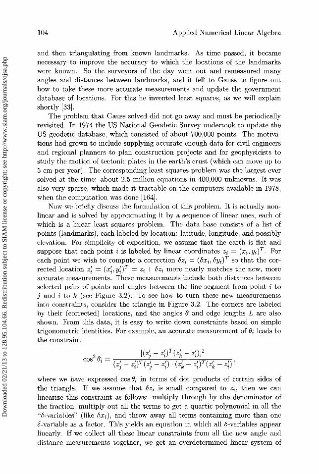
Now we briefly discuss the formulation of this problem. It is actually non-linear and is solved by approximating it by a sequence of linear ones, each ofwhich is a linear least squares problem. The data base consists of a list ofpoints (landmarks), each labeled by location: latitude, longitude, and possiblyelevation. For simplicity of exposition, we assume that the Barth is flat andsuppose that each point i is labeled by linear coordinates zi = (xi, yi) T . Foreach point we wish to compute a correction 5zi = ( 6xi, Syi) T so that the cor-rected location z = (xi, y')T = zi + 5zi more nearly matches the new, moreaccurate measurements. These measurements include both distances betweenselected pairs of points and angles between the line segment from point i toj and i to k (see Figure 3.2). To see how to turn these new measurementsinto constraints, consider the triangle in Figure 3.2. The corners are labeledby their (corrected) locations, and the angles 0 and edge lengths L are alsoshown. From this data, it is easy to write down constraints based on simpletrigonometric identities. For example, an accurate measurement of ei leads to

the constraint

COS2 Bi = [(zj - zi) T (zk - zi)] 2

(zj - zi)T ( j - zi) . ( zk - zi)T (zk - zi)

where we have expressed cos ei in terms of dot products of certain sides of

the triangle. If we assume that 6zi is small compared to zi, then we canlinearize this constraint as follows: multiply through by the denominator ofthe fraction, multiply out all the terms to get a quartic polynomial in all the"6-variables" (like 5xi), and throw away all terms containing more than oneS-variable as a factor. This yields an equation in which all 6-variables appearlinearly. If we collect all these linear constraints from all the new angle anddistance measurements together, we get an overdetermined linear system of

Dow

nloa

ded

02/2

1/13

to 1

28.9

5.10

4.66

. Red

istr

ibut

ion

subj

ect t

o SI

AM

lice

nse

or c

opyr

ight

; see

http

://w

ww

.sia

m.o

rg/jo

urna

ls/o

jsa.

php

Linear Least Squares Problems 105

Z'j=(Xj Yj )

z'k=(x'k,Yk)

z'^=(X'1 ,Yi )

Fig. 3.2. Constraints in updating a geodetic database.

equations for all the S-variables. We wish to find the smallest corrections, i.e.,the smallest values of Sxi, etc., that most nearly satisfy these constraints. This

is a least squares problem. o

Later, after we introduce more machinery, we will also show how image

compression can be interpreted as a least squares problem (see Example 3.4).

3.2. Matrix Factorizations That Solve the Linear Least

Squares Problem

The linear least squares problem has several explicit solutions that we nowdiscuss:

1. normal equations,

2. QR decomposition,

3. SVD,

4. transformation to a linear system (see Question 3.3).

The first method is the fastest but least accurate; it is adequate when thecondition number is small. The second method is the standard one and costsup to twice as much as the first method. The third method is of most use on anill-conditioned problem, i.e., when A is not of full rank; it is several times moreexpensive again. The last method lets us do iterative refinement to improvethe solution when the problem is ill-conditioned. All methods but the thirdcan be adapted to deal efficiently with sparse matrices [33]. We will discusseach solution in turn. We assume initially for methods 1 and 2 that A has full

column rank n.

Dow

nloa

ded

02/2

1/13

to 1

28.9

5.10

4.66

. Red

istr

ibut

ion

subj

ect t

o SI

AM

lice

nse

or c

opyr

ight

; see

http

://w

ww

.sia

m.o

rg/jo

urna

ls/o

jsa.

php

106

Applied Numerical Linear Algebra

3.2.1. Normal Equations

To derive the normal equations, we look for the x where the gradient of II Ax —

bI12 = (Ax — b)T (Ax — b) vanishes. So we want

0 = lim (A(x + e) — b) T (A(x + e) — b) — (Ax — b) T (Ax — b)

e- o IICII22eT (ATAx — AT b) + eTATAe=

e 0 I1e112

The second term e e^2 e< IIAIIéI112112 = JIAII2IIeII2 approaches 0 as e goes to

0, so the factor AT Ax—AT b in the first term must also be zero, or ATAx = ATb.

This is a system of n linear equations in n unknowns, the normal equations.

Why is x = (ATA) —I ATb the minimixer of IIAx — bI12? We can note thatthe Hessian ATA is positive definite, which means that the function is strictlyconvex and any critical point is a global minimum. Or we can complete thesquare by writing x' = x + e and simplifying

(Ax'—b) T (Ax'—b) = (Ae + Ax — b)T(Ae + Ax — b)

= (Ae)T (Ae) + (Ax — b) T (Ax — b)

+2(Ae) T (Ax — b)

= IIAeII2+IIAx—bII2+26T (ATAx —ATb )

= IIAe112+ IIAx —bI12•

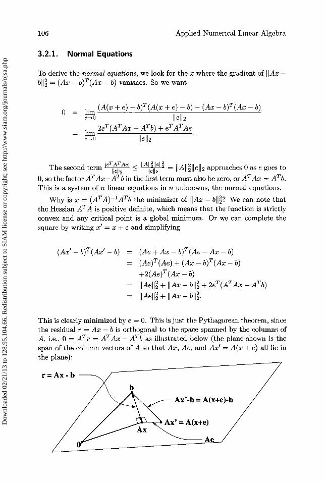
This is clearly minimized by e = 0. This is just the Pythagorean theorem, sincethe residual r = Ax — b is orthogonal to the space spanned by the columns of

A, i.e., 0 = ATr = ATAx — ATb as illustrated below (the plane shown is thespan of the column vectors of A so that Ax, Ae, and Ax' = A(x + e) all lie in

the plane):

r=

Dow

nloa

ded

02/2

1/13

to 1

28.9

5.10

4.66

. Red

istr

ibut

ion

subj

ect t

o SI

AM

lice

nse

or c

opyr

ight

; see

http

://w

ww

.sia

m.o

rg/jo

urna

ls/o

jsa.

php


Since ATA is symmetric and positive definite, we can use the Choleskydecomposition to solve the normal equations. The total cost of computing

ATA, AT b, and the Cholesky decomposition is n2m + 3 n3 + 0(n2 ) flops. Since

m > n, the n2m cost of forming ATA dominates the cost.

3.2.2. QR Decomposition

THEOREM 3.1. QR decomposition. Let A be m-by-n with m >_ n. Supposethat A has full column rank. Then there exist a unique m-by-n orthogonalmatrix Q (QT Q = In) and a unique n-by-n upper triangular matrix R withpositive diagonale r22 > 0 such that A = QR.

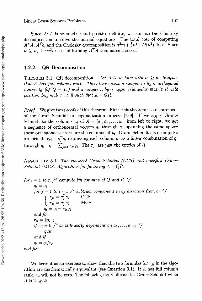
Proof. We give two proofs of this theorem. First, this theorem is a restatementof the Gram—Schmidt orthogonalization process [139]. If we apply Gram—Schmidt to the columns ai of A = [al, a2, ... , an] from left to right, we geta sequence of orthonormal vectors ql through q„ spanning the same space:these orthogonal vectors are the columns of Q. Gram—Schmidt also computescoefficients rei = q^ ai expressing each column ai as a linear combination of ql

through qi: a2 = =1 r^jqj. The rei are just the entries of R.

ALGORITHM 3.1. The classical Gram—Schmidt (CGS) and modified Gram—Schmidt (MGS) Algorithms for factoring A = QR:

for i = 1 to n /* compute ith columns of Q and R */

qi = ai

for j = 1 to i — 1 /* subtract component in qj direction from ai */rj2 = q ai CGS

r^2 = q^ qi MGSqZ = qz — rjjqj

end forrij = Il qi 112if r22 = 0 /* a2 is linearly dependent on al,... ,al */

quitend if

qz = gi/r22end for

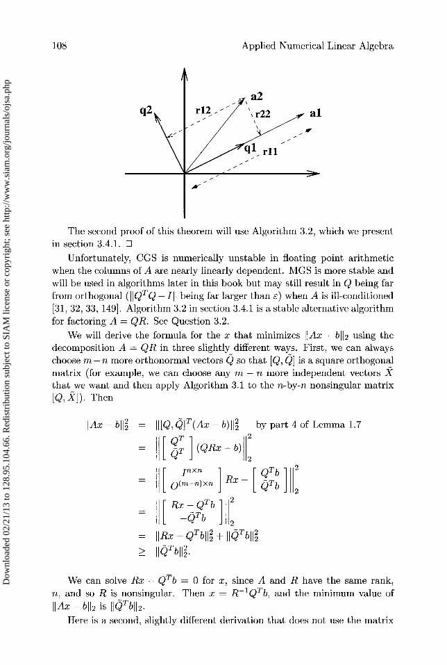
We leave it as an exercise to show that the two formulas for rei in the algo-rithm are mathematically equivalent (see Question 3.1). If A has full columnrank, r22 will not be zero. The following figure illustrates Gram—Schmidt whenA is 2-by-2:

Dow

nloa

ded

02/2

1/13

to 1

28.9

5.10

4.66

. Red

istr

ibut

ion

subj

ect t

o SI

AM

lice

nse

or c

opyr

ight

; see

http

://w

ww

.sia

m.o

rg/jo

urna

ls/o

jsa.

php

108


The second proof of this theorem will use Algorithm 3.2, which we presentin section 3.4.1. ❑

Unfortunately, CGS is numerically unstable in floating point arithmeticwhen the columns of A are nearly linearly dependent. MGS is more stable andwill be used in algorithmslater in this book but may still result in Q being farfrom orthogonal (I QT Q - I being far larger than s) when A is ill-conditioned[31, 32, 33, 149]. Algorithm 3.2 in section 3.4.1 is a stable alternative algorithmfor factoring A = QR. See Question 3.2.

We will derive the formula for the x that minimizes lAx - bil2 using thedecomposition A = QR in three slightly different ways. First, we can alwayschoose m - n more orthonormal vectors Q so that [Q, Q] is a square orthogonalmatrix (for example, we can choose any m - n more independent vectors Xthat we want and then apply Algorithm 3.1 to the n-by-n nonsingular matrix[Q, X]). Then

Ax — bI I2 = II [Q, Q] T (Ax — b) I I2 by part 4 of Lemma 1.7_ QT 1 (QRx - b) 2

J 2

= I O(m n)xn J Rx — 1 L QTb 1 2

L `w ]M2

— [ Rx Q QT b 1I2

J2

= IIRx—QTbii2+IIQTbiI2IIQTb112

We can solve Rx - QTb = 0 for x, since A and R have the same rank,n, and so R is nonsingular. Then x = R-1 QTb, and the minimum value of

II Ax — bil 2 is II QT bll 2 .Here is a second, slightly different derivation that does not use the matrix

Dow

nloa

ded

02/2

1/13

to 1

28.9

5.10

4.66

. Red

istr

ibut

ion

subj

ect t

o SI

AM

lice

nse

or c

opyr

ight

; see

http

://w

ww

.sia

m.o

rg/jo

urna

ls/o

jsa.

php


Q. Rewrite Ax — b as

Ax—b = QRx—b=QRx—(QQT +I—QQT )b

= Q(Rx — QTb) — (1— QQT ) b.

Note that the vectors Q(Rx — QTb) and (I — QQT)b are orthogonal, be-

cause (Q(Rx — QT b)) T ((I — QQT )b) = (Rx — QT b) T [QT (I — QQT )]b = (Rx —

QT b) T [0] b = 0. Therefore, by the Pythagorean theorem,

IIAx — bllá = IIQ(Rx — QTb) II2+ 1I(I— QQT )b112

= 1iRx—QTbII2 + II(I— QQT )bII2,

where we have used part 4 of Lemma 1.7 in the form I I Qy I12 = I1 y 112. This sum

of squares is minimized when the first term is zero, i.e., x = R-1 QTb.Finally, here is a third derivation that starts from the normal equations

solution:

x = (ATA) —I AT b_ (RTQTQR) -1 RT QT b = (RTR)- 1 RTQTb

= R—lR—TRTQTb = R-1QTb.

Later we will show that the cost of this decomposition and subsequent leastsquares solution is 2n2m — 2 n3 , about twice the cost of the normal equations

if m » n and about the same if m = n.

3.2.3. Singular Value Decomposition

The SVD is a very important decomposition which is used for many purposesother than solving least squares problems.

THEOREM 3.2. SVD. Let A be an arbitrary m-by-n matrix with m >_ n. Thenwe can write A = UEVT , where U is m-by-n and satisfies UTU = I, V is n-by-n and satisfies VTV = I, and E = diag(al, ... , an ), where cr > • • • > un > 0.The columns ul, ... ,u of U are called left singular vectors. The columns

vn of V are called right singular vectors. The ui are called singular

values. (If m < n, the SVD is defined by considering AT.)

A geometric restatement of this theorem is as follows. Given any m-by-n

matrix A, think of it as mapping a vector x E R n to a vector y = Ax E IRm .

Then we can choose one orthogonal coordinate system for R (where the unitaxes are the columns of V) and another orthogonal coordinate system for R m

(where the units axes are the columns of U) such that A is diagonal (E), i.e.,

maps a vector x = Ei 1 f32v2 to y = Ax = 1 aj/3 ui. In other words, any

matrix is diagonal, provided that we piek appropriate orthogonal coordinate

systems for its domain and range.

Dow

nloa

ded

02/2

1/13

to 1

28.9

5.10

4.66

. Red

istr

ibut

ion

subj

ect t

o SI

AM

lice

nse

or c

opyr

ight

; see

http

://w

ww

.sia

m.o

rg/jo

urna

ls/o

jsa.

php


Proof of Theorem 3.2. We use induction on m and n: we assume that the SVDexists for (m — 1)-by-(n — 1) matrices and prove it for m-by-n. We assumeA $ 0; otherwise we can take E = 0 and let U and V be arbitrary orthogonalmatrices.

The basic step occurs when n = 1 (since m >_ n). We write A = UEVT

with U =A/IIAII2,E=IIAII2, and V=1.For the induction step, choose v so 11 v 112 = 1 and I A I I 2= I I Av I I 2 > 0. Such

a v exists by the definition of IIAII2 = max11 112=1 IIAvhI2. Let u = ^Âv112 , which

is a unit vector. Choose Ü and V so that U = [u, U] is an m-by-m orthogonalmatrix, and V = [v, V] is an n-by-n orthogonal matrix. Now write

T T nTATUTAV=I

r UT]•A•[v V]=

[UTAvUTAV].

Then

UTAv = (Av)T (Av) = IIAvII2 = IIAvhl2 = IIAII2 - U

IIAvhl2 IIAvII2

and UT Av = UT u I I Av I 12 = 0. We claim UT Ç/ = 0 too because otherwise

or = IIAII2 = IIUTAVII2 > II[1,0,...,0]UTAVII2 = II [UIuTAV]II 2 > a, a contra-diction. (We have used part 7 of Lemma 1.7.)

So UT AV = [ 0 ÜAV ] = [ 0 q ] • We may now apply the induction

hypothesis to A to get A = U1E1VT , where Ui is (m — 1)-by-(n — 1), E, is(n — 1)-by-(n — 1), and Vl is (n — 1)-by-(n — 1). So

0 1_1 0 Q 0 1 0UTAV=CO U

1 ^ 1 VT J[ 0 U1 ] [0 El] [ 0 V1 ]

or

A=\U 0 UlJ/ L 0 E1J (v[

0 Vl]/T

which is our desired decomposition. ❑

The SVD has a large number of important algebraic and geometric prop-erties, the most important of which we state here.

THEOREM 3.3. Let A = UEVT be the SVD of the m-by-n matrix A, wherem > n. (There are analogous results for m < n.)

1. Suppose that A is symmetrie, with eigenvalues Xz and orthonormal eigen-vectors ui. In other words A = UAUT is an eigendecomposition of A,with A = diag(\1, ... , ) ), U = [ul, ... , u,], and UUT = I. Then anSVD of A is A = UEVT , where oj = IXiI and vz = sign7i)ui, wheresign(0) = 1.

Dow

nloa

ded

02/2

1/13

to 1

28.9

5.10

4.66

. Red

istr

ibut

ion

subj

ect t

o SI

AM

lice

nse

or c

opyr

ight

; see

http

://w

ww

.sia

m.o

rg/jo

urna

ls/o

jsa.

php


111

2. The eigenvalues of the symmetrie matrix A TA are o•2. The right singularvectors vz are corresponding orthonormal eigenvectors.

3. The eigenvalues of the symmetrie matrix AA T are a2 and m — n zeroes.The left singular vectors ui are corresponding orthonormal eigenvectors

for the eigenvalues Q2. One can take any m — n other orthogonal vectorsas eigenvectors for the eigenvalue 0.

4. Let H = [ Á óT ], where A is square and A = UEVT is the SVD of A.

Let E = diag(o-1, ...,o ), U = [u1,...,un], and V = [vl,...,v]. Thenthe 2n eigenvalues of H are ±uj, with corresponding unit eigenvectors

2 [ ±ui

5. If A has full rank, the solution of mini IlAx — bil2 is x = VE —l UTb.

6. IIAII2 = cr i . If A is square and nonsingular, then II A-1 11 2 1 — o-n and

JIAI12.11A—'112 = "n

7. Suppose Ui > ... > aT > aT+i = ... = an = 0. Then the rank of A is r.The null space of A, i.e., the subspace of vectors v such that Av = 0, isthe space spanned by columns r + 1 through n of V: span(vr+1 , . .. , vn ).The range space of A, the subspace of vectors of the foren Aw for all w,is the space spanned by columns 1 through r of U: span(ul, ... , Ur ).

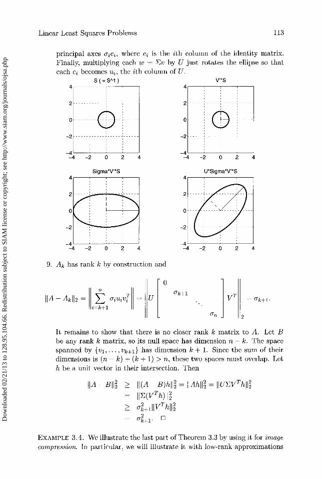
8. Let S'— ' be the unit sphere in Rn: Sn-1 = {x E R 11XJ12 = 1}.Let A • Sn-1 be the image of Sn-1 under A: A • Sn— ' = {Ax x ER7 and 11X11 2 = 1}. Then A • Sn -1 is an ellipsoid centered at the originof R, with principal axes cru.

9. Write V = [vl , v2 , ... , vn] and U = [ut, u2,. . . , u?], so A = UEVT

r 1 uiuivl (a sum of rank-1 matrices). Then a matrix of rank k < n

closest to A (measured with I1 12) is Ak = Ek_ 1 o-iuivT, and IIA — Ak112 =Qk+1• We may also write Ak = UEkVT , where Ek = diag(ul, ... , Qk, 0,...,0).

Proof.

1. This is true by the definition of the SVD.

2. ATA = V EUT UEVT = V E2 VT . This is an eigendecomposition of ATA,with the columns of V the eigenvectors and the diagonal entries of E 2

the eigenvalues.

3. Choose an m-by-(m—n) matrix Ü so that [U, U] is square and orthogonal.Then write

AAT = U^VTVÛT = U^ 2 UT = [U, ü] [2 0 0]

[U^ü]T

Dow

nloa

ded

02/2

1/13

to 1

28.9

5.10

4.66

. Red

istr

ibut

ion

subj

ect t

o SI

AM

lice

nse

or c

opyr

ight

; see

http

://w

ww

.sia

m.o

rg/jo

urna

ls/o

jsa.

php


This is an eigendecomposition of AAT .

4. See Question 3.14.

5. II Ax - bII2 = II UEVT x - b1I2. Since A has full rank, so does E, and thusE is invertible. Now let [U, U] be square and orthogonal as above so

T l 2

UEVT x — bII2 = [ UT J (UEVT x — b)2

EVTTbT b 1 112

J 2

= II EVT x - UT bII2 + I UTblIz•

This is minimized by making the first term zero, i.e., x = VE-l UTb.

6. It is ciear from its definition that the two-norm of a diagonal matrix isthe largest absolute entry on its diagonal. Thus, by part 3 of Lemma 1.7,

IIAII2 = II UT AV II2 = IIr-II2 = ai and Al 2 = II VT A-1 UII2 = IIy-_ l II2 =-in

7. Again choose an m-by-(m - n) matrix Ü so that the m-by-m matrixU = [U, U] is orthogonal. Since U and V are nonsingular, A and UT AV =

^nXn

[ ^^n^_n^Xn ] - E have the same rank namely, r—by our assumption

about E. Also, v is in the null space of A if and only if VT v is in the nullspace of UT AV = E, since Av = 0 if and only if UT AV (VT v) = 0. Butthe null space of E is clearly spanned by columns r + 1 through n of then-by-n identity matrix In , so the null space of A is spanned by V timesthese columns, i.e., v,. + l through vn . A similar argument shows that therange space of A is the same as U times the range space of UT AV =i.e., U times the first r columns of I„t , or ul through ur .

8. We "build" the set A • Sn- ' by multiplying by one factor of A = UEVT

at a time. The figure below illustrates what happens when

A = [ 3113J

2 -1 /2 -2 -1 /2 4 0 2-1/2 -2 -1 /2 T

_[ 2-1/2 2-1/2 ][ 0 2 [ 2-1/2 2-1/2

UEVT .

Assume for simplicity that A is square and nonsingular. Since V isorthogonal and so maps unit vectors to other unit vectors, VT • Sn-1 =Sn-1 . Next, since v E S'^-1 if and only if IIvII2 = 1, w E ESn -1 if andonly if IIE -1 w1I2 = 1 or Ei 1(wz/ai) 2 = 1. This defines an ellipsoid with

Dow

nloa

ded

02/2

1/13

to 1

28.9

5.10

4.66

. Red

istr

ibut

ion

subj

ect t

o SI

AM

lice

nse

or c

opyr

ight

; see

http

://w

ww

.sia

m.o

rg/jo

urna

ls/o

jsa.

php


113

principal axes Qiei, where e2 is the ith column of the identity matrix.

Finally, multiplying each w = Ev by U just rotates the ellipse so thateach ei becomes ui, the ith column of U.

s(= S^1) V'*S4

4

2

2

0

0

-2 -2

-4 -4-4 -2 0 2 4 -4 -2 0 2 4

Sigma*V'*S U*Sigma*V'*S4

4

2

2 ------ - --,--- -- --

0

0 ----- ------

-2 -2 ---- ----- ---------

-4 -4

-4 -2 0 2 4 -4 -2 0 2 4

9. Ak has rank k by construction and

0

IIA — AkII2 = Ê uiuivz = U VT = ak+1 .Ê

7 '7k+1

i=k+1

Orn 2

It remains to show that there is no closer rank k matrix to A. Let Bbe any rank k matrix, so its null space has dimension n — k. The spacespanned by {vl, ... , vk+l} has dimension k + 1. Since the sum of theirdimensions is (n — k) + (k + 1) > n, these two spaces must overlap. Let

h be a unit vector in their intersection. Then

IIA—B1I2 > II(A—B)h1I2 = IIAh1I2 = IIUEVT h1Iz

= II (VT h)112

'— ak+lIIVT hII22

_ ak+1

EXAMPLE 3.4. We illustrate the last part of Theorem 3.3 by using it for imagecompression. In particular, we will illustrate it with low-rank approximations

Dow

nloa

ded

02/2

1/13

to 1

28.9

5.10

4.66

. Red

istr

ibut

ion

subj

ect t

o SI

AM

lice

nse

or c

opyr

ight

; see

http

://w

ww

.sia

m.o

rg/jo

urna

ls/o

jsa.

php


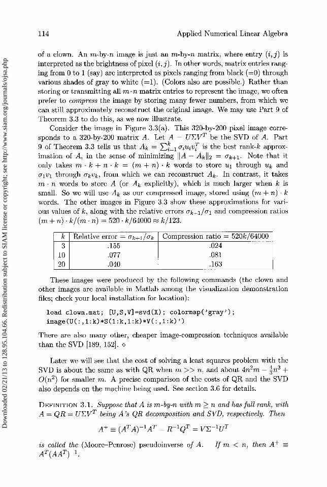
of a clown. An m-by-n image is just an m-by-n matrix, where entry (i, j) isinterpreted as the brightness of pixel (i, j). In other words, matrix entries rang-ing from 0 to 1 (say) are interpreted as pixels ranging from black (=0) throughvarious shades of gray to white (=1). (Colors also are possible.) Rather thanstoring or transmitting all m • n matrix entries to represent the image, we oftenprefer to compress the image by storing many fewer numbers, from which wecan still approximately reconstruct the original image. We may use Part 9 ofTheorem 3.3 to do this, as we now illustrate.

Consider the image in Figure 3.3(a). This 320-by-200 pixel image corre-sponds to a 320-by-200 matrix A. Let A = UEVT be the SVD of A. Part

9 of Theorem 3.3 tells us that Ak = Ik_ 1 ojuivT is the best rank-k approx

imation of A, in the sense of minimizing I I A — Ak I I2 = Uk+l • Note that it

only takes m • k + n • k = (m + n) • k words to store ul through Uk and

alvl through akvk, from which we can reconstruct Ak. In contrast, it takes

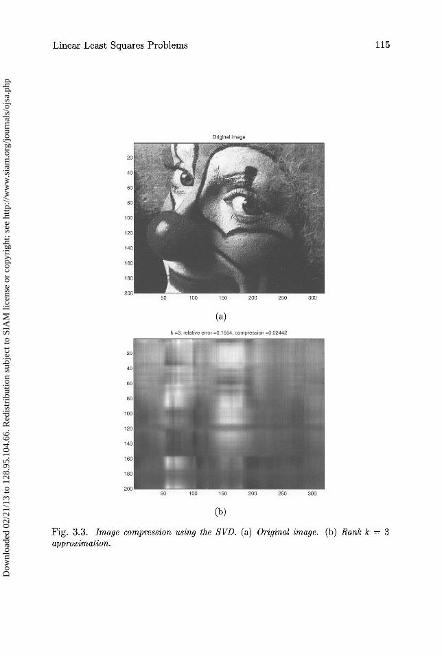
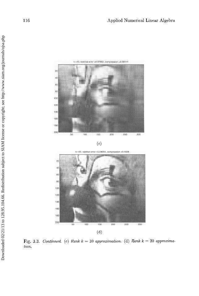
m • n words to store A (or Ak explicitly), which is much larger when k issmall. So we will use Ak as our compressed image, stored using (m + n) • kwords. The other images in Figure 3.3 show these approximations for vari-ous valnes of k, along with the relative errors ak+1 /a1 and compression ratios

(m + n) • k/(m • n) = 520.k/64000 k/123.

k Relative error = 0-k+1 /ak Compression ratio = 520k/64000

3 .155 .02410 .077 .081

20 .040 .163

These images were produced by the following commands (the clown andother images are available in Matlab among the visualization demonstrationfiles; check your local installation for location):

load clown.mat; [U,S,V]=svd(X); colormap('gray');image(U(:,1:k)*S(1:k,1:k)*V(:,1:k)')

There are also many other, cheaper image-compression techniques available

than the SVD [189, 152]. o

Later we will see that the cost of solving a least squares problem with theSVD is about the same as with QR when m » n, and about 4n2 m — 3n3 +

O(n2 ) for smaller m. A precise comparison of the costs of QR and the SVD

also depends on the machine being used. See section 3.6 for details.

DEFINITION 3.1. Suppose that A is m -by-n with m > n and has full rank, withA = QR = UEVT being A's QR decomposition and SVD, respectively. Then

A+ _ (ATA) — 'AT = R-1 QT = VE —l UT

is called the (Moore-Penrose) pseudoinverse of A. If m < n, then A+AT(AAT) -1.

Dow

nloa

ded

02/2

1/13

to 1

28.9

5.10

4.66

. Red

istr

ibut

ion

subj

ect t

o SI

AM

lice

nse

or c

opyr

ight

; see

http

://w

ww

.sia

m.o

rg/jo

urna

ls/o

jsa.

php


(a)

(b)

Fig. 3.3. Image compression using the SVD. (a) Original image. (b) Rank k = 3approzimation.

Dow

nloa

ded

02/2

1/13

to 1

28.9

5.10

4.66

. Red

istr

ibut

ion

subj

ect t

o SI

AM

lice

nse

or c

opyr

ight

; see

http

://w

ww

.sia

m.o

rg/jo

urna

ls/o

jsa.

php

116


(c)

(d)

Fig. 3.3. Continued. (c) Rank k = 10 approxioration. (d) Rank k = 20 approxima-tion.

Dow

nloa

ded

02/2

1/13

to 1

28.9

5.10

4.66

. Red

istr

ibut

ion

subj

ect t

o SI

AM

lice

nse

or c

opyr

ight

; see

http

://w

ww

.sia

m.o

rg/jo

urna

ls/o

jsa.

php


The pseudoinverse lets us write the solution of the full-rank, overdeter-mined least squares problem as simply x = A+b. If A is square and full rank,this formula reduces to x = Ab as expected. The pseudoinverse of A iscomputed as pinv (A) in Matlab. When A is not full rank, the Moore—Penrosepseudoinverse is given by Definition 3.2 in section 3.5.

3.3. Perturbation Theory for the Least Squares Problem

When A is not square, we define its condition number with respect to the2-norm to be i2(A) - 0-„,ax(A)/Qmin(A). This reduces to the usual conditionnumber when A is square. The next theorem justifies this definition.

THEOREM 3.4. Suppose that A is m-by-n with m >_ n and has full rank. Sup-pose that x minimizes Ax—bII2. Let r = Ax—b be the residual. Let x minimize

II (A + 6A)i — (b + 5b) 11 2 . Assume e - max( i6Ai 2 Il 5bll2 ) < 1 __ --in(A)JI I1 ijb112 /r2(` Qmax(A)

Then

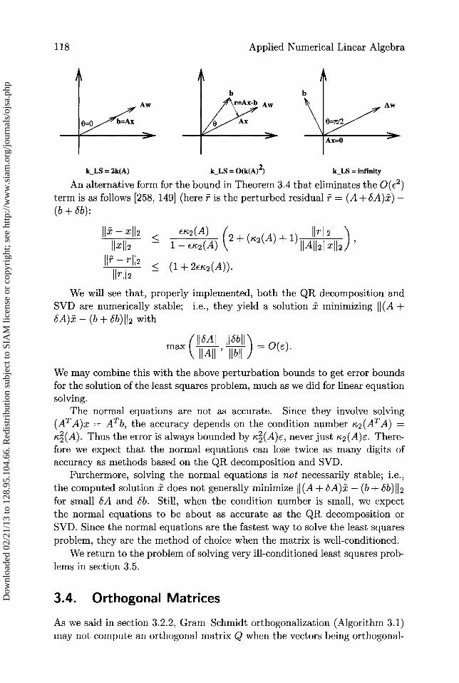
lxp x l2 112 < E f2 (A) +tan0 . r.2(A) } +O(e 2 ) - e • kLS + O ( E2 ) ,

where sin 0 = 11 ILbII2 . In other words, 0 is the angle between the vectors b and

Ax and measures whether the residual norm IIr112 is large (near Ilbil) or small(near 0). kLS is the condition number for the least squares problem.

Sketch of Proof. Expand x = ((A + SA)T (A + bA)) —1 (A + bA)T (b + bb) inpowers of SA and bb, and throw away all but the linear terms in SA and bb. O

We have assumed that e • r,2 (A) <1 for the same reason as in the derivationof bound (2.4) for the perturbed solution of the square linear system Ax = b:it guarantees that A + SA has full rank so that x is uniquely determined.

We may interpret this bound as follows. If 0 is 0 or very small, then theresidual is small and the effective condition number is about 2k2(A), much likeordinary linear equation solving. If 0 is not small but not close to r/2, theresidual is moderately large, and then the effective condition number can be

much larger: K(A). If 9 is close to ir/2, so the true solution is nearly zero,then the effective condition number becomes unbounded even if k2 (A) is small.These three cases are illustrated below. The right-hand picture makes it easyto see why the condition number is infinite when 9 = 7r/2: in this case thesolution x = 0, and almost any arbitrarily small change in A or b will yield anonzero solution x, an "infinitely” large relative change.

Dow

nloa

ded

02/2

1/13

to 1

28.9

5.10

4.66

. Red

istr

ibut

ion

subj

ect t

o SI

AM

lice

nse

or c

opyr

ight

; see

http

://w

ww

.sia

m.o

rg/jo

urna

ls/o

jsa.

php

118


k_LS = 2k(A) k_LS = O(k(A)2 k_LS = infinity

An alternative form for the bound in Theorem 3.4 that eliminates the O(e 2 )term is as follows [258, 149] (here r is the perturbed residual r = (A+SA)x) —(b + bb):

IIx — x112 < Er,2(A)(2+ (Yv2(A) + 1) Ilrll2

11x112 1-a2(A) ^JA11211x112 IIr — r11 2 < (1 + 26r2(A)).

11rl12 -

We will see that, properly implemented, both the QR decomposition andSVD are numerically stable; i.e., they yield a solution x minimizing II (A +A)— (b + bb) lI2 with

ilbAIl lk5bmax ij) =O(6).C IIAI1 1^b^^

We may combine this with the above perturbation bounds to get error boundsfor the solution of the least squares problem, much as we did for linear equationsolving.

The normal equations are not as accurate. Since they involve solving(AT A)x = AT b, the accuracy depends on the condition number k2 (ATA) _rc2(A). Thus the error is always bounded by t2(A)E, never just r,2(A)E. There-fore we expect that the normal equations can lose twice as many digits ofaccuracy as methods based on the QR decomposition and SVD.

Furthermore, solving the normal equations is not necessarily stable; i.e.,the computed solution x does not generally minimize I (A + SA) — (b + 5b) 112for small SA and 5b. Still, when the condition number is small, we expectthe normal equations to be about as accurate as the QR decomposition orSVD. Since the normal equations are the fastest way to solve the least squaresproblem, they are the method of choice when the matrix is well-conditioned.

We return to the problem of solving very ill-conditioned least squares prob-lems in section 3.5.

3.4. Orthogonal Matrices

As we said in section 3.2.2, Gram—Schmidt orthogonalization (Algorithm 3.1)may not compute an orthogonal matrix Q when the vettors being orthogonal-

Dow

nloa

ded

02/2

1/13

to 1

28.9

5.10

4.66

. Red

istr

ibut

ion

subj

ect t

o SI

AM

lice

nse

or c

opyr

ight

; see

http

://w

ww

.sia

m.o

rg/jo

urna

ls/o

jsa.

php


ized are nearly linearly dependent, so we cannot use it to compute the QRdecomposition stably.

Instead, we base our algorithms on certain easily computable orthogonalmatrices called Householder relections and Givens rotations, which we canchoose to introduce zeros into vectors that they multiply. Later we will showthat any algorithm that uses these orthogonal matrices to introduce zerosis automatically stable. This error analysis will apply to our algorithms forthe QR decomposition as well as many SVD and eigenvalue algorithms inChapters 4 and 5.

Despite the possibility of nonorthogonal Q, the MGS algorithm has im-portant uses in numerical linear algebra. (There is little use for its less stableversion, CGS.) These uses include finding eigenvectors of symmetrie tridiagonalmatrices using bisection and inverse iteration (section 5.3.4) and the Arnoldiand Lanczos algorithms for reducing a matrix to certain "condensed" forms(sections 6.6.1, 6.6.6, and 7.4). Arnoldi and Lanczos algorithms are used asthe basis of algorithms for solving sparse linear systems and finding eigenval-ues of sparse matrices. MGS can also be modified to solve the least squaresproblem stably, but Q may still be far from orthogonal [33].

3.4.1. Householder Transformations

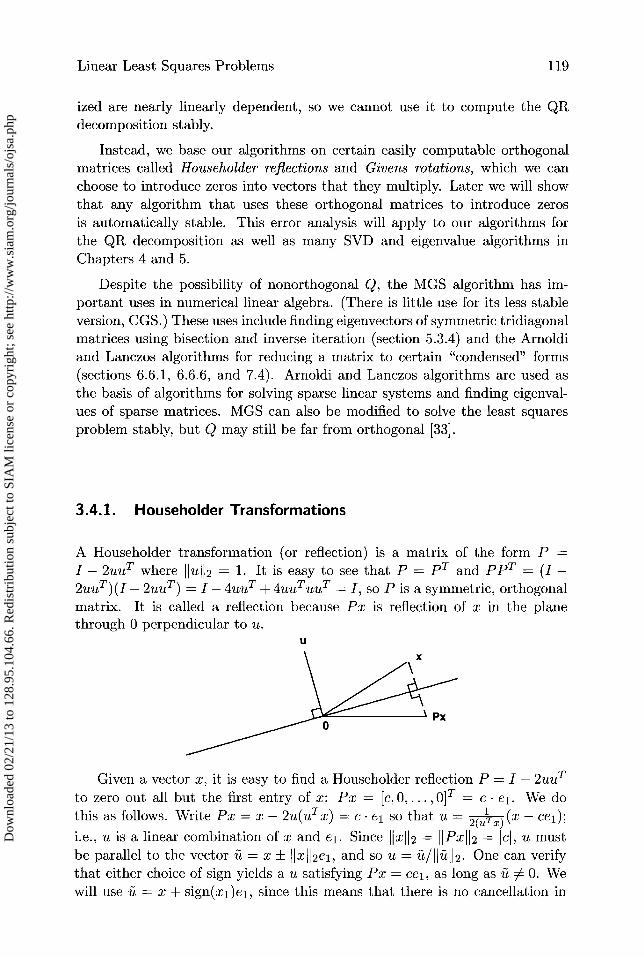
A Householder transformation (or reflection) is a matrix of the form P =I — 2uuT where hÛ112 = 1. It is easy to see that P = PT and ppT = (I —2uuT ) (I — 2uuT ) = I — 4uuT + 4uuT uuT = I, so P is a symmetrie, orthogonalmatrix. It is called a reflection because Px is reflection of x in the planethrough 0 perpendicular to u.

u

Given a vector x, it is easy to find a Householder reflection P = I — 2uuT

to zero out all but the first entry of x: Px = [c, 0, ... , 0] T = c • Cl. We dothis as follows. Write Px = x — 2u(uTx) = c. el so that u = 2(u x) (x — cel);

i.e., u is a linear combination of x and e l . Since 11x11 2 = IIPxI1 2 = lci, u mustbe parallel to the vector u = x + hlxhI2e1, and so u = u/IIuIH2. One can verifythat either choice of sign yields a u satisfying Px = cel, as long as u 0. Wewill use ü = x + sign(x1)ei, since this means that there is no cancellation in

Dow

nloa

ded

02/2

1/13

to 1

28.9

5.10

4.66

. Red

istr

ibut

ion

subj

ect t

o SI

AM

lice

nse

or c

opyr

ight

; see

http

://w

ww

.sia

m.o

rg/jo

urna

ls/o

jsa.

php

120


computing the first component of ü. In summary, we get

xl + sign(x1) • IIXII2X2 uu = with u = Iu II2xn

We write this as u = House(x). (In practice, we can store ü instead of u to savethe work of computing u, and use the formula P = I — (2 /IluI12)uuT insteadofP=I-2uuT .)

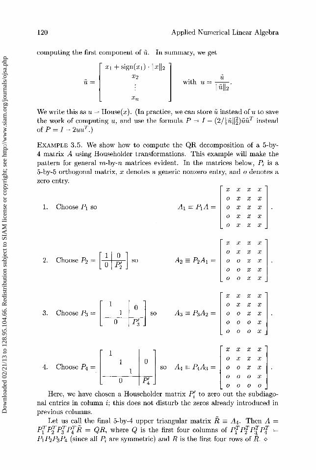
EXAMPLE 3.5. We show how to compute the QR decomposition of a 5-by-4 matrix A using Householder transformations. This example will make thepattern for general m-by-n matrices evident. In the matrices below, PZ is a5-by-5 orthogonal matrix, x denotes a generic nonzero entry, and o denotes azero entry.

1. Choose Pl so

2. Choose P2 = [0 p, so2J

1 03. Choose P3 = 1 so

0 P

XXX X

o x x xAl=PlA= o x x x

0 XXX

0 XXX

XXX X

0 XXX

A2-P2A1= 0 0 X X

00 x x00 x x

XXX X

0 XXX

A3-P3A2= 0 0 X X

O O O X

O O O X

1 XXX X

1 0 0 XXX

4. Choose P4 = 1 so A4 - P4A3 = 0 0 X X

0P4 0 0 0 xO O O O

Here, we have chosen a Householder matrix P' to zero out the subdiago-nal entries in column i; this does not disturb the zeros already introduced inprevious columns.

Let us call the final 5-by-4 upper triangular matrix R - A4. Then A =Pi P2 P3 PR = QR, where Q is the first four columns of PP2 P3 P4P1P2P3P4 (since all PZ are symmetric) and R is the first four rows of R. o

Dow

nloa

ded

02/2

1/13

to 1

28.9

5.10

4.66

. Red

istr

ibut

ion

subj

ect t

o SI

AM

lice

nse

or c

opyr

ight

; see

http

://w

ww

.sia

m.o

rg/jo

urna

ls/o

jsa.

php


Here is the general algorithm for QR decomposition using Householdertransformations.

ALGORITHM 3.2. QR factorization using Householder reflections:

for i = 1 to min(m — 1, n)uz = Heuse(A(i : m, i))P'= I-2uiuTA(i:m,i:n)=PZA(i:m,i:n)

end for

Here are some more implementation details. We never need to form PZexplicitly but just multiply

(I-2uiuT)A(i:m,i:n)=A(i:m,i: n)-2ui(uTA(i:m,i:n)),

which costs less. To store Pi, we need only ui, or ui and Iui. These canbe stored in column i of A; in fact it need not be changed! Thus QR can be"overwritten" on A, where Q is stored in factored form Pl ... Pn_1 i and PZ isstored as ui below the diagonal in column i of A. (We need an extra array oflength n for the top entry of ui, since the diagonal entry is occupied by Rii.)

Recall that to solve the least squares problem min IAx—b112 using A = QR,we need to compute QTb. This is done as follows: QTb = PnPn_i . • Pi b, sowe need only keep multiplying b by Pi, P2,. . . , Pn :

for i=1 ton-y=-2•uTb(i:m)b(i : m) = b(i : m) + 7ui

end for

The cost is n dot products ry = —2 • uT b and n "saxpys" b + ^/ui. The costof computing A = QR this way is 2n2 m — 3n3 , and the subsequent cost ofsolving the least squares problem given QR is just an additional O(mn).

The LAPALK routine for solving the least squares problem using QR issgels. Just as Gaussian elimination can be reorganized to use matrix-matrixmultiplication and other Level 3 BLAS (see section 2.6), the same can be donefor the QR decomposition; see Question 3.17. In Matlab, if the m-by-n matrixA has more rows than columns and b is m by 1, A\b solves the least squaresproblem. The QR decomposition itself is also available via [Q,R]=qr(A).

3.4.2. Givens Rotations

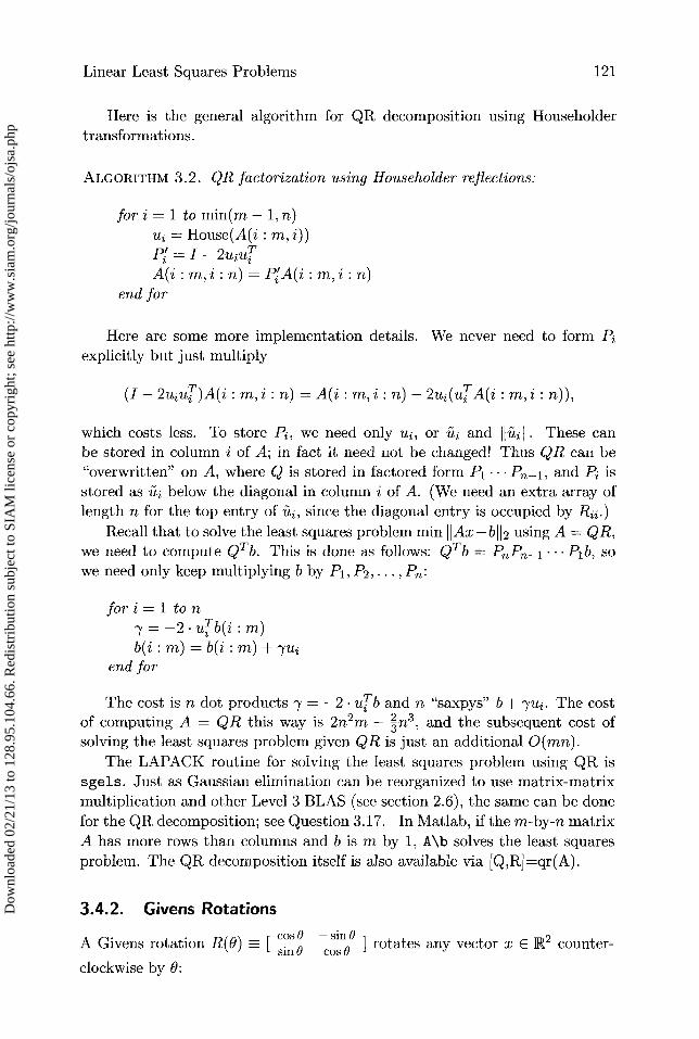
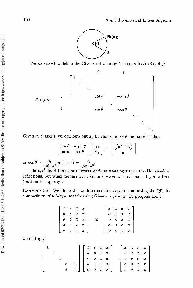
A Givens rotation R(0) _ [ cos B — sin B ]sin B cos B

rotates any vector x E R2 counter-

clockwise by 0:

Dow

nloa

ded

02/2

1/13

to 1

28.9

5.10

4.66

. Red

istr

ibut

ion

subj

ect t

o SI

AM

lice

nse

or c

opyr

ight

; see

http

://w

ww

.sia

m.o

rg/jo

urna

ls/o

jsa.

php

122


R(e)x

x

We also need to define the Givens rotation by 0 in coordinates i and j:

i j

1 1

cos B — sin BR(i, j, B)

7 sin 9 cos B

1

L 1

Given x, i, and j, we can zero out x by choosing cos 0 and sin 0 so that

cos 0 — sin 9 xi_ ^X2 + X^[ sine cos B ] [ x j , 6

or cos 0 = x z and sin 0 =X2+x3 2?+X^

The QR algorithm using Givens rotations is analogous to using Householderreflections, but when zeroing out column i, we zero it out one entry at a time(bottom to top, say).

EXAMPLE 3.6. We illustrate two intermediate steps in computing the QR de-composition of a 5-by-4 matrix using Givens rotations. To progress from

X x x x X X X X

0 X X X 0 X X X

0 0 X x to o 0 X X

00 x X o 0 o X

00 x X o 0 o X

we multiply

X X X X X X X X

0 X X X 0 X X X

00 x X = 00 x X

c —s 0 0 X X 0 0 X X

s C 00 x x 000 X

Dow

nloa

ded

02/2

1/13

to 1

28.9

5.10

4.66

. Red

istr

ibut

ion

subj

ect t

o SI

AM

lice

nse

or c

opyr

ight

; see

http

://w

ww

.sia

m.o

rg/jo

urna

ls/o

jsa.

php


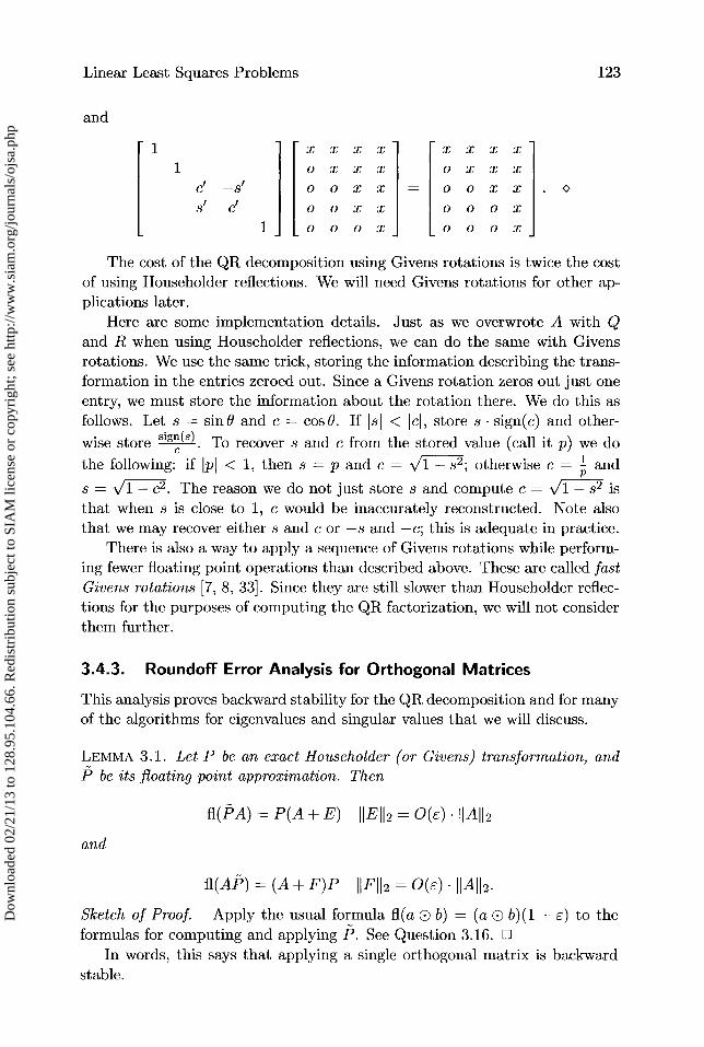
and

1 XXX x XXXI

1 0 XXX 0 XXX

C1 —S1 00 x x = 00 x x o

s' c' 0 0 x x 0 0 0 x1 o o o x o 0 o X

The cost of the QR decomposition using Givens rotations is twice the costof using Householder reflections. We will need Givens rotations for other ap-plications later.

Here are some implementation details. Just as we overwrote A with Qand R when using Householder reflections, we can do the same with Givensrotations. We use the same trick, storing the information describing the trans-formation in the entries zeroed out. Since a Givens rotation zeros out just oneentry, we must store the information about the rotation there. We do this asfollows. Let s = sin0 and c = cosO. If IsI < iei, store s • sign(c) and other-

wise store s ' gn (s) . To recover s and c from the stored value (call it p) we do

the following: if Ipi < 1, then s = p and c = T— s 2 ; otherwise c = 1 and

s = 1 — c2 . The reason we do not just store s and compute c = sf1 — s2 isthat when s is close to 1, c would be inaccurately reconstructed. Note alsothat we may recover either s and c or —s and —c; this is adequate in practice.

There is also a way to apply a sequence of Givens rotations while perform-ing fewer floating point operations than described above. These are called fastGivens rotations [7, 8, 33]. Since they are still slower than Householder reflec-tions for the purposes of computing the QR factorization, we will not considerthem further.

3.4.3. Roundoff Error Analysis for Orthogonal Matrices

This analysis proves backward stability for the QR decomposition and for manyof the algorithms for eigenvalues and singular values that we will discuss.

LEMMA 3.1. Let P be an exact Householder (or Givens) transformation, andP be its floating point approximation. Then

fl(PA) = P(A + E) hJEil2 = 0(e) . JIAI12

and

fl(AP) = (A + F)P IJFI12 = 0 (e) . hIAll2.

Sketch of Proof. Apply the usual formula fl(a O b) = (a O b)(1 + e) to theformulas for computing and applying P. See Question 3.16. ❑

In words, this says that applying a single orthogonal matrix is backwardstable.

Dow

nloa

ded

02/2

1/13

to 1

28.9

5.10

4.66

. Red

istr

ibut

ion

subj

ect t

o SI

AM

lice

nse

or c

opyr

ight

; see

http

://w

ww

.sia

m.o

rg/jo

urna

ls/o

jsa.

php


THEOREM 3.5. Consider applying a sequence of orthogonal transformationsto Ao. Then the computed product is an exact orthogonal transformation ofAo + 6A, where IISAII2 = 0(r)IIA112• In other words, the entire computation isbackward stable:

fl(f f _1 ... PiAoQ,Q2 ... Q^) =P P,(Ao+E)Qi...Q^

with I I E I I2 = i • 0(E) - I I A I I2 • Here, as in Lemma 3.1, Pi and Qi are floatingpoint orthogonal matrices and PZ and Qi are exact orthogonal matrices.

Proof. Let P^ - P3_ • • Pl and Q Q1 • • • Q. We wish to show thatfl(PjA^_1Qj) = Pj(A+E^)Q for some (IEÎI2 = jO(s)IIAII2• We use

Lemma 3.1 recursively. The result is vacuously true for j = 0. Now assumethat the result is true for j — 1. Then we compute

B = fl(PÂ^- 1 )

= Pj(A^_l+E') byLemma3.1

= Pj(Pj_1(A+ E^_1)Q^_1 + E') by induction

= P^(A+E^-1+PT lE^Q^ 1)Q^-1

P^ (A + E")Q^-1,

where

E"112 = IIE^—i + P?' 1E'Q? 1II2 <— IIE^—ilH2 + II PT IE'Qj 1II2= IIE^—1 II2 + IIE'II2= jO(E)IIAII2

since IIE^_ i ii 2 = (j — 1 ) 0 (e)IIAII2 and IIE'II2 = O(E)IIAII2. Postmultiplicationby Q is handled in the same way. ❑

3.4.4. Why Orthogonal Matrices?

Let us consider how the error would grow if we were to multiply by a sequence ofnonorthogonal matrices in Theorem 3.5 instead of orthogonal matrices. Let Xbe the exact nonorthogonal transformation and X be its floating point approx-imation. Then the usual floating point error analysis of matrix multiplicationtells us that

fl(XA) = XA+ E = X(A+X -1E) - X(A+ F),

where IIEII2 < O(e)IIXII2 . IIAII2 and so IIFII2 < IIX -1 112 ' IIEII2 <_ 0(E) • r-2(X)

IIAII2•So the error I I E I 12 is magnified by the condition number i2 (X) >_ 1. In a

larger product Xk • • • X,AY, ... Yk the error would be magnified by [ji k2(XZ) •k2 (Y). This factor is minimized if and only if all Xi and Y are orthogonal (orstalar multiples of orthogonal matrices), in which case the factor is one.

Dow

nloa

ded

02/2

1/13

to 1

28.9

5.10

4.66

. Red

istr

ibut

ion

subj

ect t

o SI

AM

lice

nse

or c

opyr

ight

; see

http

://w

ww

.sia

m.o

rg/jo

urna

ls/o

jsa.

php


3.5. Rank-Deficient Least Squares Problems

So far we have assumed that A has full rank when minimizing liAx — bII2.What happens when A is rank deficient or "close" to rank deficient? Suchproblems arise in practice in many ways, such as extracting signals from noisydata, solution of some integral equations, digital image restoration, comput-ing inverse Laplace transforms, and so on [141, 142]. These problems arevery ill-conditioned, so we will need to impose extra conditions on their so-lutions to make them well-conditioned. Making an ill-conditioned problemwell-conditioned by imposing extra conditions on the solution is called regular-ization and is also done in other fields of numerical analysis when ill-conditionedproblems arise.

For example, the next proposition shows that if A is exactly rank deficient,then the least squares solution is not even unique.

PROPOSITION 3.1. Let A be m-by-n with m > n and rank A = r < n. Thenthere is an n — r dimensional set of vectors x that minimize IAx — bII2•

Proof. Let Az = 0. Then if x minimizes lI Ax — b1I2, so does x + z. ❑

Because of roundof in the entries of A, or roundofi during the computation,it is most often the case that A will have one or more very small computedsingular values, rather than some exactly zero singular values. The next propo-sition shows that in this case, the unique solution is likely to be very large and iscertainly very sensitive to error in the right-hand side b (see also Theorem 3.4).

PROPOSITION 3.2. Let o-min = crmin(A), the smallest singular value of A. As-Sume Amin > 0. Then

1. if x minimizes lAx — bil2i then x1 2 >_ lunbl/amin , where un is the lastcolumn of U in A = UEVT .

2. changing b to b + bb can change x to x + bx, where 6X112 is as large as

Il bb 1I2 /Umin

In other words, if A is nearly rank deficient (Am in is small), then the solu-tion x is ill-conditioned and possibly very large.

Proof. For part 1, x = A+b = VE —l UTb, so 11x112 = (IE —l UTblI2 >I (E —l UT b)m,I = IunbJ /crmin. For part 2, choose bb parallel to u,. ❑

We begin our discussion of regularization by showing how to regularizean exactly rank-deficient least squares problem: Suppose A is m-by-n withrank r < n. Within the (n — r)-dimensional solution space, we will look forthe unique solution of smallest norm. This solution is characterized by thefollowing proposition.

Dow

nloa

ded

02/2

1/13

to 1

28.9

5.10

4.66

. Red

istr

ibut

ion

subj

ect t

o SI

AM

lice

nse

or c

opyr

ight

; see

http

://w

ww

.sia

m.o

rg/jo

urna

ls/o

jsa.

php

126


PROPOSITIoN 3.3. When A is exactly singular, the x that minimize 11 Ax — b 112can be characterized as follows. Let A = UEVT have rank r < n, and writethe SVD of A as

A = [Ui, U2] L Ol 0 J [V1, V2] T = U1E1VT (3.1)

where E 1 is r x r and nonsingular and Ui and Vl have r columns. Let o, =

Qmin(i), the smallest nonzero singular value of A. Then

1. all solutions x can be written x = V1Ei 1 Ul b+V2z, z an arbitrary vector.

2. the solution x has minimal norm IIx112 precisely when z = 0, in whichcase x = V1 Ei'Ul b and 11x112 < I1b11 2 /a.

3. changing b to b + Sb can change the minimal norm solution x by at mostIISb11 2 /a.

In other words, the norm and condition number of the unique minimal normsolution x depend on the smallest nonzero singular value of A.

Proof. Choose Ü so [U, U] = [U1, U2, Ü] is an m x m orthogonal matrix. Then

IIAx — bil = II[U,U] T (Ax—b)112UT 2

= Uz (UiiV1Tx_b)iiiiUT 112

E1V2'x — UTb 1112= U

UT b 112

= IIF-1VTx— U12 b112+ IIU2 b112+ IIUTb112.

1. 1 I Ax — b112 is minimized when E 1 V1T x= UTb, or x = V1 i 1 Ul b+ V2zsince V1TV2z = 0 for all z.

2. Since the columns of Vl and V2 are mutually orthogonal, the Pythagoreantheorem implies that Ilxll2 = IIVir-1 1 U1 bll2 + IIV2z112, and this is mini-mized by z = 0.

3. Changing b by bb changes x by at most I I Vi E 1 1 Ui bb I I 2< I I F- 1 1 1 12 I I Sb l i 2=Il5bll 2 /cî. ❑

Proposition 3.3 tells us that the minimum norm solution x is unique andmay be well-conditioned if the smallest nonzero singular value is not too small.This is key to a practical algorithm, discussed in the next section.

Dow

nloa

ded

02/2

1/13

to 1

28.9

5.10

4.66

. Red

istr

ibut

ion

subj

ect t

o SI

AM

lice

nse

or c

opyr

ight

; see

http

://w

ww

.sia

m.o

rg/jo

urna

ls/o

jsa.

php


EXAMPLE 3.7. Suppose that we are doing.medical research on the effect of acertain drug on blood sugar level. We collect data from each patient (numberedfrom i = 1 to m) by recording his or her initial blond sugar level (a2,1), finalblood sugar level (bi), the amount of drug administered (ai,2), and other med-ical quantities, including body weights on each day of a week-long treatment(az,3 through ai,9). In total, there are n < m medical quantities measured foreach patient. Our goal is to predict bi given ai,1 through az,„ and we formulatethis as the least squares problem min, ilAx — bil2. We plan to use x to predictthe final blond sugar level b of future patient j by computing the dot product

i:k=1 a^kxk.

Since people's weight generally does not change significantly from day today, it is likely that columns 3 through 9 of matrix A, which contain theweights, are very similar. For the sake of argument, suppose that columns3 and 4 are identical (which may be the case if the weights are rounded tothe nearest pound). This means that matrix A is rank deficient and thatxp = [0, 0, 1, —1,0,. , 0] T is a right null vector of A. So if x is a (minimumnorm) solution of the least squares problem min, liAx — bil2i then x + /3x0 isalso a (nonminimum norm) solution for any scalar 0, including, say, ,Q = 0 andQ = 106 . Is there any reason to prefer one value of 0 over another? The value106 is clearly not a good one, since future patient j, who gains one poundbetween days 1 and 2, will have that difference of one pound multiplied by106 in the predictor Ek a^kxk of final blond sugar level. It is much morereasonable to choose 0 = 0, corresponding to the minimum norm solution x.0

For further justification of using the minimum norm solution for rank-deficient problems, see [141, 142].

When A is square and nonsingular, the unique solution of Ax = b is ofcourse b = A-1x. If A has more rows than columns and is possibly rank-deficient, the unique minimum-norm least squares solution may be similarlywritten b = A+b, where the Moore—Penrose pseudoinverse A+ is defined asfollows.

DEFINITION 3.2. (Moore—Penrose pseudoinverse A+ for possibly rank-deficientA)

Let A = UEVT = U1 E 1 VT as in equation (3.1). Then A+ - V1Ei 1 U1 .This is also written A+ = VTE+U, where E+ _ [ ol 0

0 ]+ = [ E1 0 ]'

So the solution of the least squares problem is always x = A+b, and whenA is rank deficient, x has minimum norm.

Dow

nloa

ded

02/2

1/13

to 1

28.9

5.10

4.66

. Red

istr

ibut

ion

subj

ect t

o SI

AM

lice

nse

or c

opyr

ight

; see

http

://w

ww

.sia

m.o

rg/jo

urna

ls/o

jsa.

php

128


3.5.1. Solving Rank-Deficient Least Squares Problems Using theSVD

Our goal is to compute the minimum norm solution x, despite roundof. Inthe last section, we saw that the minimal norm solution was unique and had acondition number depending on the smallest nonzero singular value. Therefore,computing the minimum norm solution requires knowing the smallest nonzerosingular value and hence also the rank of A. The mail difficulty is that therank of a matrix changes discontinuously as a function of the matrix.

For example, the 2-by-2 matrix A = diag(1, 0) is exactly singular, and itssmallest nonzero singular value is o = 1. As described in Proposition 3.3, theminimum norm least squares solution to min., IlAx — bil2 with b = [1, 11 T isx = [1, 0] T , with condition number 1/Q = 1. But if we make an arbitrarilytiny perturbation to get A = diag(1, c), then o drops to E and x = [l, l/ E] T

becomes enormous, as does its condition number 1 /E. In general, roundofi willmake such tiny perturbations, of magnitude O(e)IIAII2• As we just saw, thiscan increase the condition number from 1/Q to 1/e.

We deal with this discontinuity algorithmically as follows. In general eachcomputed singular value Qi satisfies

— oij < O(--) IIAII2. This is a consequenteof backward stability: the computed SVD will be the exact SVD of a slightlydifferent matrix: A = UÊVT = A + SA, with IISA11 = 0 ( 5) . IIAII. (This isdiscussed in detail in Chapter 5.) This means that any &Z < O(e)1IA112 canbe treated as zero, because roundoff makes it indistinguishable from 0. In theabove 2-by-2 example, this means we would set the E in A to zero before solvingthe least squares problem. This would raise the smallest nonzero singular valuefrom E to 1 and correspondingly decrease the condition number from 1/E to1/o- = 1.

More generally, let tol be a user-supplied measure of uncertainty in the dataA. Roundofi implies that tol >_ e • 11 A 1 , but it may be larger, depending on thesource of the data in A. Now set & = Qi if &i > tol, and &i = 0 otherwise. LetE = diag(& ). We call UEVT the truncated SVD of A, because we have setsingular values smaller than tol to zero. Now we solve the least squares problemusing the truncated SVD instead of the original SVD. This is justified sinceII UÉVT — UÊVT 112 = IIU(E — E)VT pb 2 < tol; i.e., the change in A caused bychanging each Qi to Qi is less than the user's inherent uncertainty in the data.The motivation for using E instead of E is that of all matrices within distantetol of E, E maximizes the smallest nonzero singular value a. In other words, itminimizes both the norm of the minimum norm least squares solution x and its

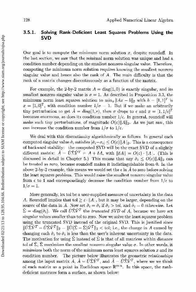
condition number. The picture below illustrates the geometric relationshipsamong the input matrix A, A = UEVT , and A = UEVT , where we we thinkof each matrix as a point in Euclidean space IRm'n. In this space, the rank-deficient matrices form a surface, as shown below:

Dow

nloa

ded

02/2

1/13

to 1

28.9

5.10

4.66

. Red

istr

ibut

ion

subj

ect t

o SI

AM

lice

nse

or c

opyr

ight

; see

http

://w

ww

.sia

m.o

rg/jo

urna

ls/o

jsa.

php


trices

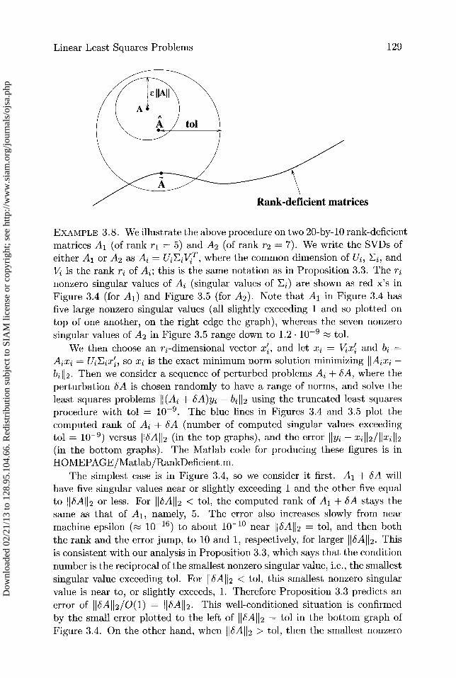
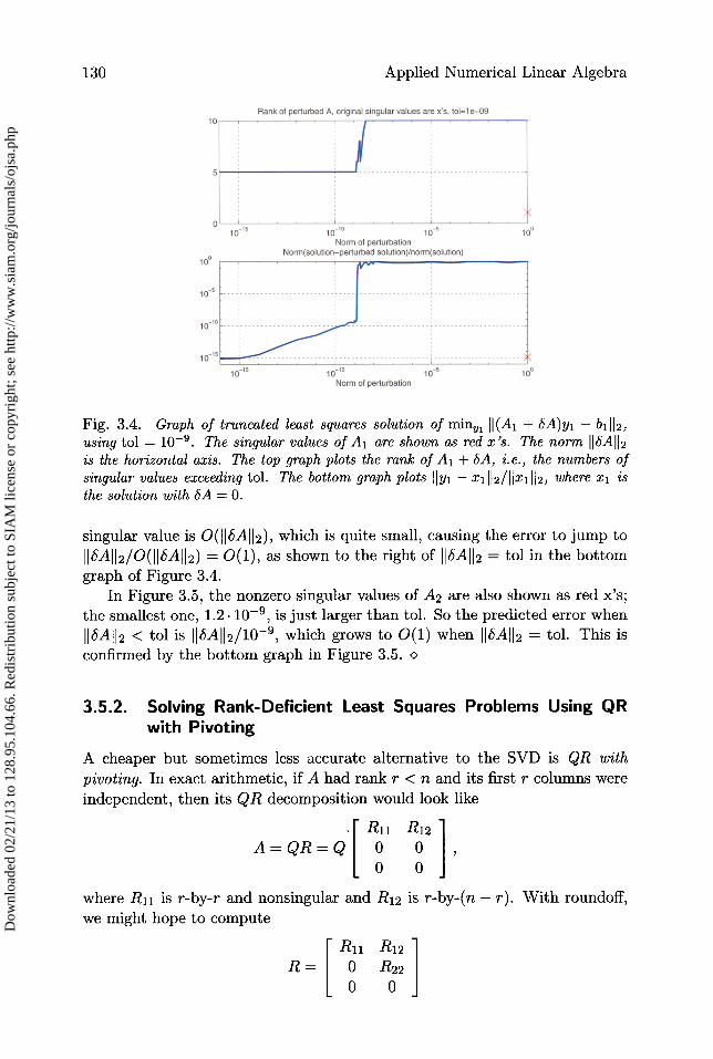
EXAMPLE 3.8. We illustrate the above procedure on two 20-by-10 rank-deficientmatrices A l (of rank rl = 5) and A2 (of rank r2 = 7). We write the SVDs of

either Al or A2 as Ai = UiE where the common dimension of UZ, E i , and

U is the rank ri of AZ; this is the same notation as in Proposition 3.3. The r2nonzero singular values of Ai (singular values of Ej) are shown as red x's inFigure 3.4 (for A1) and Figure 3.5 (for A2). Note that Al in Figure 3.4 basfive large nonzero singular values (all slightly exceeding 1 and so plotted ontop of one another, on the right edge the graph), whereas the seven nonzero

singular values of A2 in Figure 3.5 range down to 1.2 • 10 -9 tol.

We then choose an ri-dimensional vector xi, and let x, = Uxi and bi =Aixi = Ui E ixi, so x2 is the exact minimum norm solution minimizing IIAixz —b2 II2. Then we consider a sequence of perturbed problems Ai + SA, where the

perturbation SA is chosen randomly to have a range of norms, and solve the

least squares problems (Ai + SA)y2 — bi li 2 using the truncated least squares

procedure with tol = 10 -9 . The blue lines in Figures 3.4 and 3.5 plot thecomputed rank of Ai + SA (number of computed singular values exceedingtol = 10-9 ) versus IISAH2 (in the top graphs), and the error I^y2 — xiJI2/1jxj112(in the bottom graphs). The Matlab code for producing these figures is inHOMEPAGE/Matlab/RankDeficient.m.

The simplest case is in Figure 3.4, so we consider it first. Al + SA willhave five singular values near or slightly exceeding 1 and the other five equal

to IIAII2 or less. For SA 2 < tol, the computed rank of Al + 6A stays thesame as that of A 1 , namely, 5. The error also increases slowly from nearmachine epsilon ( 10 -16 ) to about 10 — '° near 16A112 = tol , and then both

the rank and the error jump, to 10 and 1, respectively, for larger 116A1H. This

is consistent with our analysis in Proposition 3.3, which says that the condition

number is the reciprocal of the smallest nonzero singular value, i.e., the smallestsingular value exceeding tol. For 16A112 < tol, this smallest nonzero singular

value is near to, or slightly exceeds, 1. Therefore Proposition 3.3 predicts anerror of 116A112/O(1) = ÎM112. This well-conditioned situation is confirmedby the small error plotted to the left of II6A2 = tol in the bottom graph ofFigure 3.4. On the other hand, when IA2 > tol, then the smallest nonzero

Dow

nloa

ded

02/2

1/13

to 1

28.9

5.10

4.66

. Red

istr

ibut

ion

subj

ect t

o SI

AM

lice

nse

or c

opyr

ight

; see

http

://w

ww

.sia

m.o

rg/jo

urna

ls/o

jsa.

php


Fig. 3.4. Graph of truncated least squares solution of min„, II(Al + SA)yl - b1112,using tol = 10-9 . The singular values of Al are shown as red x's. The norm 116A112is the horizontal axis. The top graph plots the rank of Al + SA, i.e., the numbers ofsingular values exceeding tol. The bottom graph plots IIyl - x1112/11x1112, where xl isthe solution with SA = 0.

singular value is O(lISAII2), which is quite small, causing the error to jump to

IIbAII2/o(IISA112) = 0(1), as shown to the right of 1ISA112 = tol in the bottomgraph of Figure 3.4.

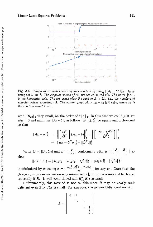
In Figure 3.5, the nonzero singular values of A2 are also shown as red x's;the smallest one, 1.2. 10 -9 , is just larger than tol. So the predicted error whenIISAII 2 < tol is IISAII2/10-9 , which grows to 0(1) when I16A112 = tol. This isconfirmed by the bottom graph in Figure 3.5. o

3.5.2. Solving Rank-Deficient Least Squares Problems Using QRwith Pivoting

A cheaper but sometimes less accurate alternative to the SVD is QR withpivoting. In exact arithmetic, if A had rank r < n and its first r columns wereindependent, then its QR decomposition would look like

Rij R12A=QR=Q 0 0

0 0

where R11 is r-by-r and nonsingular and R12 is r-by-(n - r). With roundoff,we might hope to compute

Rij R12R= 0 R22

0 0

Dow

nloa

ded

02/2

1/13

to 1

28.9

5.10

4.66

. Red

istr

ibut

ion

subj

ect t

o SI

AM

lice

nse

or c

opyr

ight

; see

http

://w

ww

.sia

m.o

rg/jo

urna

ls/o

jsa.

php


Fig. 3.5. Graph of truncated least squares solution of miny2 lI(A2 + SA)y2 — b2112,using tol = 10 -9 . The singular values of A2 are shown as red x's. The norm 116A112is the horizontal axis. The top graph plots the rank of A2 + SA, i.e., the numbers ofsingular values exceeding tol. The bottom graph plots 11y2 — x2112/11x2112, where x2 isthe solution with bA = 0.

with I I R22 112 very small, on the order of e I I A I I2 • In this case we could just setR22 = 0 and minimize 11 Ax — b I 1 2 as follows: let [Q, Q] be square and orthogonalso that

IIAx — bII2 =ir T L QT (Ax—b)

]12= r RxQQTb 2

z IL 2= IIRx — QT bi12 + 11QTbIi2•

Write Q = [Q1, Q2] and x = [ x1 ] conformally with R = [ Rll R12 1 soX2 0 0

that

IIAx — b1I2 = (IR11x1 + R12 x2 — Qi bII2 + IIQz bII2 + I IQT bII2

is minimized by choosing x = [ R111iQ1 b2 R12x2) 1 for any x2. Note that the

choice x2 = 0 does not necessarily minimize I I x 2, but it is a reasonable choice,especially if Rll is well-conditioned and R111 R12 is small.

Unfortunately, this method is not reliable since R may be nearly rankdeficient even if no R22 is small. For example, the n-by-n bidiagonal matrix

21

A =. 1

12

Dow

nloa

ded

02/2

1/13

to 1

28.9

5.10

4.66

. Red

istr

ibut

ion

subj

ect t

o SI

AM

lice

nse

or c

opyr

ight

; see

http

://w

ww

.sia

m.o

rg/jo

urna

ls/o

jsa.

php


has Am in (A) ti 2 — ', but A = Q • R with Q = I and R = A, and no R22 is small.To deal with this failure to recognize rank deficiency, we may do QR with

column pivoting. This means that we factorize AP = QR, P being a permuta-

tion matrix. This idea is that at step i (which ranges from 1 to n, the numberof columns) we select from the unfinished part of A (columns i to n and rows

i to m) the column of largest norm and exchange it with the ith column. Wethen proceed to compute the usual Householder transformation to zero outcolumn i in entries i + 1 to m. This pivoting strategy attempts to keep Rll aswell-conditioned as possible and R22 as small as possible.

EXAMPLE 3.9. If we compute the QR decomposition with column pivotingto the last example (.5 on the diagonal and 1 on the superdiagonal) withn = 11, we get R11,11 = 4.23. 10 -4 , a reasonable approximation to min(A)

3.66.10-4 . Note that R„„ > O-min(A) since Qm in (A) is the norm of the smallestperturbation that can lower the rank, and setting R^,n, to 0 lowers rank. o

One can show only a Rf(A) 2n but usually Rnn is a reasonable approx-

imation to Qmin (A). The worst case, however, is as bad as worst-case pivotgrowth in GEPP.

More sophisticated pivoting schemes than QR with column pivoting, calledrank-revealing QR algorithms, have been a subject of much recent study. Rank-revealing QR algorithms that detect rank more reliably and sometimes alsofaster than QR with column pivoting have been developed [28, 30, 48, 50, 109,126, 128, 150, 196, 236]. We discuss them further in the next section.

QR decomposition with column pivoting is available as subroutine sgeqpfin LAPACK. LAPACK also has several similar factorizations available: RQ(sgerqf), LQ (sgelqf), and QL (sgeqlf). Future LAPACK releases willcontain improved versions of QR.

3.6. Performance Comparison of Methods for Solving

Least Squares Problems

What is the fastest algorithm for solving dense least squares problems? Asdiscussed in section 3.2, solving the normal equations is fastest, followed by

QR and the SVD. If A is quite well-conditioned, then the normal equations areabout as accurate as the other methods, so even though the normal equationsare not numerically stable, they may be used as well. When A is not well-conditioned but far from rank deficient, we should use QR.

Since the design of fast algorithms for rank-deficient least squares problemsis a current research area, it is difficult to recommend a single algorithm to use.We summarize a recent study [206] that compared the performance of severalalgorithms, comparing them to the fastest stable algorithm for the non—rank-deficient case: QR without pivoting, implemented using Householder trans-formations as described in section 3.4.1, with memory hierarchy optimizations

Dow

nloa

ded

02/2

1/13

to 1

28.9

5.10

4.66

. Red

istr

ibut

ion

subj

ect t

o SI

AM

lice

nse

or c

opyr

ight

; see

http

://w

ww

.sia

m.o

rg/jo

urna

ls/o

jsa.

php


described in Question 3.17. These comparisons were made in double preci-sion arithmetic on an IBM RS6000/590. Included in the comparison were therank-revealing QR algorithms mentioned in section 3.5.2 and various imple-mentations of the SVD (see section 5.4). Matrices of various sizes and withvarious singular value distributions were tested. We present results for twosingular value distributions:

Type 1: random matrices, where each entry is uniformly distributed from —1to 1;

Type 2: matrices with singular values distributed geometrically from 1 to e(in other words, the ith singular value is 'y, where 'y is chosen so thatryn =e).

Type 1 matrices are generally well-conditioned, and Type 2 matrices arerank-deficient. We tested small square matrices (n = m = 20) and largesquare matrices (m = n = 1600). We tested square matrices because if m issufficiently greater than n in the m-by-n matrix A, it is cheaper to do a QRdecomposition as a "preprocessing step" and then perform rank-revealing QRor the SVD on R. (This is done in LAPACK.) If m » n, then the initialQR decomposition dominates the the cost of the subsequent operations on then-by-n matrix R, and all the algorithms cost about the same.

The fastest version of rank-revealing QR was that of [30, 196]. On Type1 matrices, this algorithm ranged from 3.2 times slower than QR withoutpivoting for n = m = 20 to just 1.1 times slower for n = m = 1600. On Type 2matrices, it ranged from 2.3 times slower (for n = m = 20) to 1.2 times slower(for n = m = 1600). In contrast, the current LAPACK algorithm, dgeqpf,was 2 times to 2.5 times slower for both matrix types.

The fastest version of the SVD was the one in [58], although one based ondivide-and-conquer (see section 5.3.3) was about equally fast for n = m = 1600.(The one based on divide-and-conquer also used much less memory.) For Type1 matrices, the SVD algorithm was 7.8 times slower (for n = m = 20) to 3.3times slower (for n = m = 1600). For Type 2 matrices, the SVD algorithm was3.5 times slower (for n = m = 20) to 3.0 times slower (for n = m = 1600). Incontrast, the current LAPACK algorithm, dgelss, ranged from 4 times slower(for Type 2 matrices with n = m = 20) to 97 times slower (for Type 1 matriceswith n = m = 1600). This enormous slowdown is apparently due to memoryhierarchy effects.

Thus, we see that there is a tradeoff between reliability and speed in solv-ing rank-deficient least squares problems: QR without pivoting is fastest butleast reliable, the SVD is slowest but most reliable, and rank-revealing QRis in-between. If m » n, all algorithms cost about the same. The choice ofalgorithm depends on the relative importante of speed and reliability to theuser.

Future LAPACK releases will contain improved versions of both rank-revealing QR and SVD algorithms for the least squares problem.

Dow

nloa

ded

02/2

1/13

to 1

28.9

5.10

4.66

. Red

istr

ibut

ion

subj

ect t

o SI

AM

lice

nse

or c

opyr

ight

; see

http

://w

ww

.sia

m.o

rg/jo

urna

ls/o

jsa.

php

134


3.7. References and Other Topics for Chapter 3

The best recent reference on least squares problems is [33], which also discussesvariations on the basic problem discussed here (such as constrained, weighted,and updating least squares), different ways to regularize rank-deficient prob-lems, and software for sparse least squares problems. See also chapter 5 of[121] and [168]. Perturbation theory and error bounds for the least squaressolution are discussed in detail in [149]. Rank-revealing QR decompositionsare discussed in [28, 30, 48, 50, 126, 150, 196, 206, 236]. In particular, thesepapers examine the tradeoff between cost and accuracy in rank determination,and in [206] there is a comprehensive performance comparison of the availablemethods for rank-deficient least squares problems.

3.8. Questions for Chapter 3

QUESTION 3.1. (Easy) Show that the two variations of Algorithm 3.1, CGSand MGS, are mathematically equivalent by showing that the two formulas forrei yield the same results in exact arithmetic.

QUESTION 3.2. (Easy) This question will illustrate the difference in nu-merical stability among three algorithms for computing the QR factoriza-tion of a matrix: Householder QR (Algorithm 3.2), CGS (Algorithm 3.1),and MGS (Algorithm 3.1). Obtain the Matlab program QRStability.m fromHOMEPAGE/Matlab/QRStability.m. This program generates random matri-ces with user-specified dimensions m and n and condition number cnd, computestheir QR decomposition using the three algorithms, and measures the accuracyof the results. It does this with the residual I I A — Q • R I / I A I I , which should bearound machine epsilon E for a stable algorithm, and the orthogonality of Q^1QT • Q — I j, which should also be around E. Run this program for small ma-trix dimensions (such as m= 6 and n= 4), modest numbers of random matrices(samples= 20), and condition numbers ranging from cnd= 1 up to cnd= 10 15 .

Describe what you see. Which algorithms are more stable than others? Seeif you can describe how large JQT • Q — I^^ can be as a function of choice ofalgorithm, cnd and E.

QUESTION 3.3. (Medium; Hard) Let A be m-by-n, m > n, and have full rank.

1. (Medium) Show that [ AT A ] [

r ] _ [

b ] has a solution where x

minimizes hjAx — bil2. One reason for this formulation is that we canapply iterative refinement to this linear system if we want a more accurateanswer (see section 2.5).

2. (Medium) What is the condition number of the coefficient matrix in termsof the singular values of A? Hint: Use the SVD of A.

Dow

nloa

ded

02/2

1/13

to 1

28.9

5.10

4.66

. Red

istr

ibut

ion

subj

ect t

o SI

AM

lice

nse

or c

opyr

ight

; see

http

://w

ww

.sia

m.o

rg/jo

urna

ls/o

jsa.

php


3. (Medium) Give an explicit expression for the inverse of the coefficientmatrix, as a block 2-by-2 matrix. Hint: Use 2-by-2 block Gaussian elim-ination. Where have we previously seen the (2,1) block entry?

4. (Hard) Show how to use the QR decomposition of A to implement aniterative refinement algorithm to improve the accuracy of x.

QUESTION 3.4. (Medium) Weighted least squares: If some components of Ax-b are more important than others, we can weight them with a scale factor diand solve the weighted least squares problem min II D(Ax — b) I I2 instead, whereD has diagonal entries di. More generally, recall that if C is symmetric positivedefinite, then lxIIc - (xTCx)112 is a norm, and we can consider minimizing

Ax — bIIC• Derive the normal equations for this problem, as well as theformulation corresponding to the previous question.

QUESTION 3.5. (Medium; Z. Bai) Let A E Rnxn be positive definite. Twovectors ul and u2 are called A-orthogonal if ul Aug = 0. If U E RnxT andUT AU = I, then the columns of U are said to be A-orthonormal. Show thatevery subspace has an A-orthonormal basis.

QUESTION 3.6. (Easy; Z. Bai) Let A have the form

A= [ ]

where R is n-by-n and upper triangular, and S is m-by-n and dense. Describean algorithm using Householder transformations for reducing A to upper trian-gular form. Your algorithm should not "fill in" the zeros in R and thus requirefewer operations than would Algorithm 3.2 applied to A.

QUESTION 3.7. (Medium; Z. Bai) If A = R + uvT , where R is an upper trian-gular matrix, and u and v are column vectors, describe an efficient algorithmto compute the QR decomposition of A. Hint: Using Givens rotations, youralgorithm should take O(n2 ) operations. In contrast, Algorithm 3.2 would takeO(n3) operations.

QUESTION 3.8. (Medium; Z. Bai) Let x E R' and let P be a Householdermatrix such that Px = ± IxÎ2e1. Let G1,2 i ... , G 7 _1, be Givens rotations,and let Q = Gl,2 ... G71 _1,n . Suppose Qx = +IIxII2e1. Must P equal Q? (Youneed to give a proof or a counterexample.)

QUESTION 3.9. (Easy; Z. Bai) Let A be m-by-n, with SVD A = UEVT

Compute the SVDs of the following matrices in terms of U, E, and V:

1. (ATA)_ l

2. (ATA)-1AT

Dow

nloa

ded

02/2

1/13

to 1

28.9

5.10

4.66

. Red

istr

ibut

ion

subj

ect t

o SI

AM

lice

nse

or c

opyr

ight

; see

http

://w

ww

.sia

m.o

rg/jo

urna

ls/o

jsa.

php


3. A(ATA) -1

4. A(ATA) — 'AT

QUESTION 3.10. (Medium; R. Schreiber) Let Ak be a best rank-k approxima-tion of the matrix A, as defined in Part 9 of Theorem 3.3. Let ui be the ithsingular value of A. Show that Ak is unique if Uk > uk+1

QUESTION 3.11. (Easy; Z. Bai) Let A be m-by-n. Show that X = A+ (theMoore—Penrose pseudoinverse) minimizes II AX — III F over all n-by-m matricesX. What is the value of this minimum?

QUESTION 3.12. (Medium; Z. Bai) Let A, B, and C be matrices with di-mensions such that the product ATCBT is well defined. Let X be the set ofmatrices X minimizing I I AX B — C I I F, and let Xo be the unique member of Xminimizing IIXIIF• Show that Xo = A+CB+. Hint: Use the SVDs of A andB.

QUESTION 3.13. (Medium; Z. Bai) Show that the Moore—Penrose pseudoin-verse of A satisfies the following identities:

AA+A = A,

A+AA+ = A+,

A+A = (A+A)T ,AA+ = (AA+) T

QUESTION 3.14. (Medium) Prove part 4 of Theorem 3.3: Let

H = [ Á óT ], where A is square and A = UEVT is its SVD. Let E _diag(ui, ... ,o),), U = [ul, ... ,u], and V = [vi, ... ,v]. Prove that the 2n

eigenvalues of H are +aj, with corresponding unit eigenvectors [ v' . ]. Ex-

tend to the case of rectangular A.

QUESTION 3.15. (Medium) Let A be m-by-n, m < n, and of full rank. Thenmin II Ax — btI2 is called an underdetermined least squares problem. Show thatthe solution is an (n — m)-dimensional set. Show how to compute the uniqueminimum norm solution using appropriately modified normal equations, QRdecomposition, and SVD.

QUESTION 3.16. (Medium) Prove Lemma 3.1.

Dow

nloa

ded

02/2

1/13

to 1

28.9

5.10

4.66

. Red

istr

ibut

ion

subj

ect t

o SI

AM

lice

nse

or c

opyr

ight

; see

http

://w

ww

.sia

m.o

rg/jo

urna

ls/o

jsa.

php


QUESTION 3.17. (Hard) In section 2.6.3, we showed how to reorganize Gaus-sian elimination to perform Level 2 BLAS and Level 3 BLAS at each step inorder to exploit the higher speed of these operations. In this problem, we willshow how to apply a sequence of Householder transformations using Level 2and Level 3 BLAS.

1. Let ul, ... , ub be a sequence of vectors of dimension n, where jUiIJ2 = 1and the first i — 1 components of ui are zero. Let P = Pb • Pb_ 1 ... Pl,where PZ = I — 2uiuT is a Householder transformation. Show that thereis a b-by-b lower triangular matrix T such that P = I — UTUT , whereU = [ul, ... , ub]. In particular, provide an algorithm for computing theentries of T. This identity shows that we can replace multiplication by bHouseholder transformations Pl through Pb by three matrix multiplica-tions by U, T, and UT (plus the cost of computing T).

2. Let House(x) be a function of the vector x which returns a unit vector usuch that (I — 2uuT)x = IIxII2ei; we showed how to implement House(x)in section 3.4. Then Algorithm 3.2 for computing the QR decompositionof the m-by-n matrix A may be written as

for i = 1 mui = House(A(i : m, i))PZ = I — 2uiuT'A(i:m,i:n)=PZA(i:rn,i:n)

endfor

Show how to implement this in terms of the Level 2 BLAS in an efficientway (in particular, matrix-vector multiplications and rank-1 updates).What is the floating point operation count? (Just the high-order termsin n and m are enough.) It is sufficient to write a short program in thesame notation as above (although trying it in Matlab and comparingwith Matlab's own QR factorization are a good way to make sure thatyou are right!).

3. Using the results of step (1), show how to implement QR decompositionin terms of Level 3 BLAS. What is the operation count? This technique isused to accelerate the QR decomposition, just as we accelerated Gaussianelimination in section 2.6. It is used in the LAPACK routine sgeqrf.

QUESTION 3.18. (Medium) It is often of interest to solve constrained leastsquares problems, where the solution x must satisfy a linear or nonlinear con-straint in addition to minimizing IIAx — bil2. We consider one such problemhere. Suppose that we want to choose x to minimize lAx — bil2 subject tothe linear constraint Cx = d. Suppose also that A is m-by-n, C is p-by-n,and C has full rank. We also assume that p < n (so Cx = d is guaranteed to

Dow

nloa

ded

02/2

1/13

to 1

28.9

5.10

4.66

. Red

istr

ibut

ion

subj

ect t

o SI

AM

lice

nse

or c

opyr

ight

; see

http

://w

ww

.sia

m.o

rg/jo

urna

ls/o

jsa.

php


be consistent) and n < m + p (so the system is not underdetermined). Show

that there is a unique solution under the assumption that [ ] has full column

rank. Show how to compute x using two QR decompositions and some matrix-vector multiplications and solving some triangular systems of equations. Hint:Look at LAPACK routine sgglse and its description in the LAPACK manual[10] (NETLIB/lapack/lug/lapack_lug.html).

QUESTION 3.19. (Hard; Programming) Write a program (in Matlab or anyother language) to update a geodetic database using least squares, as describedin Example 3.3. Take as input a set of "landmarks," their approximate coordi-nates (xi, y2), and a set of new angle measurements B and distance measure-ments The output should be corrections (Sxi, Syz) for each landmark, anerror bound for the corrections, and a picture (triangulation) of the old andnew landmarks.

QUESTION 3.20. (Hard) Prove Theorem 3.4.

QUESTION 3.21. (Medium) Redo Example 3.1, using a rank-deficient leastsquares technique from section 3.5.1. Does this improve the accuracy of thehigh-degree approximating polynomials?

Dow

nloa

ded

02/2

1/13

to 1

28.9

5.10

4.66

. Red

istr

ibut

ion

subj

ect t

o SI

AM

lice

nse

or c

opyr

ight

; see

http

://w

ww

.sia

m.o

rg/jo

urna

ls/o

jsa.

php

Documents

3. Linear Least Squares Problems