3-DIMENSIONAL PLASMA FLUID MODELLING OF ISLAND FLUX TUBES IN W7-X GEOMETRY

STEFAN WEBER

Max-Planck lnstitut fiir Plasmaphysik, Teilinstitut Greifswald, EURATOM Association, Walther-Rathenau-Str. 49a, D-17489 Greifswald, Germany

1 Introduction

Modelling of the W7-X divertor and edge region presents itself with several difficulties: a fully 3-dimensional magnetic topology which automatically requires the code to have the same dimension, a complex geometry (divertor configuration), the usual large transport anisotropy perpendicular and parallel to the magnetic field and the occurrence of stochastic magnetic field regions close to the separatrix. In addition open and closed flux surfaces have to be treated within the same context.

At present 3-dimensional codes are under development for an eventually accurate modelling of the plasma edge and divertor region in stellarator devices. For W7-X two lines are persued: a fluid approach being developed at W7-X [ 1 ] and a Monte-Carlo type approach being tested at W7-AS [2].

2 Status of 3D Plasma Fluid Modelling for W7-X

To initiate fluid modelling of this region two codes have been developed for preliminary investigations: PEC3D [1] and FT3D (flux tubes in 3 dimensions), presented here.

PEC3D solves the full 3-dimensional Braginskii equations with standard sources/sinks due to ionisation and recombination together with a neutral diffusion model in a simplified, slab-like, geometry whereas FT3D solves the anisotropic Laplace equation for the electron temperature

V . (XllVll% + x•177 = 0 (1)

in the full magnetic topology with the help of magnetic coordinates. Therefore the physics is kept to the most essential but the geometry is treated without any restrictions.

PEC3D is useful for looking at the basic physics processes in 3 dimensions and Fr3D is used for the modelling of an island flux tube as they exist outside the separatrix of the standard magnetic configuration of W7-X. At present the two codes are complementary but eventually they are expected to merge into a single code which enables accurate modelling of the plasma edge region of the W7-X divertor.

3 Flux Tubes in 3 Dimensions

In the case of W7-X there are 5 closed independent island tubes winding around the Core plasma with t ~ 1. It is sufficient for the beginning to model a single one of these. In particular

Czechoslovak Journal of Physics Vol. 48 (1998), Suppl. $2 34.5

S. Weber

this might also be used as a model/'or the LHD divertor configuration where a single (m=l, n=l) island flux tube is created in the edge [3].

3.1 Geometry and the use of magnetic coordinates

Fig.1 shows the magnetic topology of the W7-X configuration and the flux tube that is

modelled.

Fig. 1. Left: the outermost flux surface of one of the five island flux tubes in the outer region of the W7-X configuration winding around the main plasma. Right: superposition of poloidal cuts of the flux

tube taken every 6~ one colour represents half a period.

Due to the very large transport anisotropy (parallel and perpendicular to the magnetic field) the choice of magnetic coordinates (s, 0, qS) is considered well adapted. 0 and 4) are generalized angle-like variables and s is the radial coordinate. The parameter range is unity for all three variables. For a detailed exposition of the construction of magnetic coordinates see [4],[5]. As can be shown the perpendicular and parallel gradient parts take the following form:

/TF~ v , , - F~I%-F'~J (~Oo + o~)

gO~ g~ 0 ] v• = vs as + . , iVY~176 + iVsl 2 ~] (2)

v s x 6 V• = - ( F ~ I + FS, J)IVsl 2 (I(9o - JOy)

VII is the gradient in the direction of the magnetic field 17, V• the gradient in the direction Vs, i.e. perpendicular to the flux surfaces and V• also being perpendicular to the magnetic field, in the direction Vs x/3 .

346 Czech. J. Phys. 48/$2 (1998)

3-dimensional plasma fluid modelling of island ...

I and J are the poloidal and toroidal currents and F~ and F:~ are the radial derivatives of the

flux functions. ~ is defined as: ~ = Up/F~. In the plasma edge it is a valid approximation to

set the toroidaI current J = 0 and also 9 r = 0 because the plasma pressure in the edge is very

small. This simplifies the above formulae.

As can be seen from the differential operators occurring in Eqn.2 the transport along the

0-direction is a mixture of parallel and perpendicular transport whereas the radial transport

(s-direction) remains pure perpendicular transport and the transport along the C-coordinate line

is pure parallel transport. In magnetic coordinates the heat flux vector has thefore the resulting

form:

go~ ] = + x . ,nvs as + i - a0/To

I I J

1 (8 • vs) 00r + x-2n (3)

+ x , v [r + a+] W~

Arranging the terms according to the three gradient directions the following expression results:

Fq,, = + x• [ 9 o` 1 B ] OT~

13 9T. + XllI 0r

The two different perpendicular transport coefficients simply account for the tact that transport

in these directions may difl'er. The perpendicular transport is anomalous. Dimensional analysis

of the equation [XII] = [X• cm-3 requires a value for n as no equation tbr the density is solved. The effective perpendicular transport coefficient X~L = X• ' n = 1017 cm -1s-1 is used for

subsequent calculations.

The parallel transport coefficient is the usual Braginskii heat conductivity with XII oc T 5/2. The resulting transport anisotropy for a typical temperature of 10 eV (see Fig. 2) is: xf___L ~ 7.0- 10 5.

X •

The equation to be solved has the simple form V �9 Fq. = O. In order to avoid applying the

rather complicated divergence operator in magnetic coordinates the equation is solved in its

integral form making use of Gauss' theorem:

L , . v . ;o, ev = Loorq,, (5)

This lends itself immediately for a numerical treatment by the Finite-Volume method where

the volume is the computational volume and the area is the surface area of each computational

cell. I.e. /'or each computational cell the following relation must hold:

6 6

O~ E / : {...}.fida,~ E [{...} �9 fi, l kAk (6) = �9 k k = l

Czech. J. Phys. 48/$2 (1998) 347

S. Weber

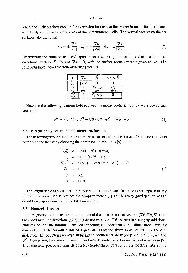
where the curly brackets contain the expression for the heat flux vector in magnetic coordinates

and the Ak are the six surface areas of the computational cells. The normal vectors on the six

surfaces take the form:

Vs VO Vr

Discretizing the equation in a FV-approach requires taking the scalar products of the three

directional vectors (/3, Vs and Vs x /3) with the surface normal vectors given above. The

following table shows the non-vanishing products.

v , IVs[ o o v__.!e 9"" B_~_ ~,r -B~ Ivol [rot Ivol J v~lvol

o B d V r o IVr

Note that the following relations hold between the metric coefficients and the surface normal

vectors:

gS* = V s . V s , gOO = VO- VO, gr162 = V r V r (8)

3.2 Simple analytical model for metric coefficients

The following prescription for the metric was extracted from the lull set of Fourier coefficients

describing the metric by choosing the dominant contributions [6]:

v ~ = - 5 3 4 - 86cos(2~-r

g,o = 5.6sin(4~-[0- r

IVsl 2 = s (43 + 37cos(4~[0 - r = j s ,

F~. = 7r

I = 882

z = 1.085

(9)

The length scale is such that the minor radius of the island flux tube is set approximately

to one. The above set determines the complete metric [7], and is a very good qualitative and

quantitative approximation to the full Fourier set.

3.3 Numerical issues

As magnetic coordinates are non-orthogonal the surface normal vectors (V0, Vr Vs) and

the coordinate line directions (e~, e~, 4 ) do not coincide. This results in setting up additional

matrices besides the minimal 7 needed for orthogonal coordinates in 3 dimensions. Writing

down in detail the various terms of Eqn.6 and using the above table results in a 15-point

molecule. The following non-vanishing metric coefficients are needed: 9% 9 ~176 9 r162 9 *0 and

g r176 Concerning the choice of freedom and interdependence of the metric coefficients see [7].

The numerical procedure consists of a Newton-Raphson iterative solver together with a fully

348 Czech. J. Phys. 48/$2 (1998)

3-dimensional plasma fluid modelling of island ...

implicit discretization scheme. Details were presented elsewhere [1].

For the calculations a mesh of 20x20x20 (O,s,(~) points was used.

3.4 Boundary conditions

The generalized angle variables 0 and ~b are assigned periodic boundary conditions in

accordance with the topology of a closed flux surface.

The s variable requires more complicated boundary conditions, s = 0 is the magnetic axis of

the island flux tube. The metric coefficients of magnetic coordinates diverge at this point so that

the boundary conditions have to be assigned at s = e > 0 such that no power flows across the

boundary (i.e. VTc = 0) and all points at s = c must have the same value, such that in the limit

s = e > 0 a unique temperature results for the island O-point.

At s = 1 ( the outermost flux surface ) a simple divertor is simulated. Its surface coincides

with a flux surface. On this divertor surface three stripes with different boundary conditions

are winding around the flux tube: an assigned high temperature (20 eV) simulating a high

temperature part of the island and ensuring a power flow into the flux tube, an assigned low

temperature (5eV) simulating a low temperature part where power is leaving the island and a no

power flow condition (VT = 0) in between the two.

3.5 Island flux tube temperature profiles

Fig. 2. shows a typical electron temperature profile of a complete flux tube in magnetic

coordinates lbr the metric given above. At present this is a formal calculation as the boundary

conditions for the divertor are not yet realistic. The reason being that the actual divertor nearly

follows the field lines so that the stripes are not at constant 0. But they can nicely be modelled

with an angle of 45 ~ in the 0 - ~b plane.

Fig. 2. Electron temperature plot [eV] of an island flux tube in magnetic coordinates; the unit cube is shown from two different angles.

Czech. J. Phys. 48/$2 (1998) 349

S. Weber: 3-dimensional plasma fluid modelling of island ...

4 Perspective for a 3D Plasma Fluid Edge Code

In a first realization of a fully 3-dimensional edge code with more or less complete physics

one would consider only the case of well-behaved flux surfaces. At a later stage one has to take

into account the occurrence of stochastic fields in the edge region. One possibility might be a

kind of hybrid code in which the stochastic regions are treated with a Monte-Carlo type code

and the orderly flux surfaces with a standard fluid code [8]. The two of them would then have to

be coupled at the appropriate cell boundaries and fluxes across these boundaries would of course

have to be conserved. Where "good" surfaces are available it makes sense to use a fluid code

as there would be no noise level. However it would be very difficult to construct field aligned

meshes for FV schemes in stochastic regions. The choice of method (fluid versus MC) has to

be governed by the prevailing magnetic topology in any particular region of the computational

domain.

So far the work has mainly concentrated on assembling primary tools and testing various

approaches to the issue of 3-dimensional plasma edge modelling. The goal, of course, is to

achieve the same standard as exemplified in the various edge codes used for tokamak transport

simulations.

These two approaches so far (PEC3D & FT3D) (full physics with simple geometry and simple

physics with full geometry) are expected to merge into a single code which enables accurate

modelling of the plasma edge region of the W7-X divertor.

5 Outlook

The next step for FT3D would be a more accurate representation of the actual divertor which

cuts through several layers of flux surfaces and also is aligned with the field lines such that a

transformation of the coordinate system (0 = - 0 + ~b) should be performed. In addition one

might want to use the full set of Fourier coefficients to describe the metric, although only small

quantitative changes are expected.

I'm thankful to S. Gori for providing me with numerical data and an illustrative figure of an W7-X

island flux tube, to C. Hennig for turning the numerical output into excellent 3D graphics and to J.

Ntihrenberg for very helpful discussions.

References

[1] S. Weber" Contrib. Plasma Phys. 38 (1998) 43.

[2] "1(. Feng etaL: J. Nuc. Mat. 241-243 (1997) 930.

[3] A. Komori et al.: Proceedings 15th Int. Conf. Plasma Phys. Contr. Nuc. Fusion Res.,

Seville, Spain 1994, IAEA-CN-60/F-P-4.

[4] J. Ntihrenberg, R. Zille: in Theory o f Fusion Plasma. Editrice Compositori 1987, p.3.

[5] W.D. D'haeseleer et aL : Flux Coordinates and Magnetic Field Structure. Springer, 199 I.

[6] J. Ntihrenberg: private communication.

[7] C. Schwab: Ph.D. Thesis 1991, Technical University Darmstadt.

[8] R. Schneider: private communication.

350 Czech. J. Phys. 48/$2 (1998)