3-DIMENSIONAL COMPUTATIONAL FLUID CELL USING DIFFERENT FUELS by SACHIN LAXMAN … · 3-dimensional computational fluid ... cell using different fuels . by . sachin laxman puthran

3-DIMENSIONAL COMPUTATIONAL FLUID

DYNAMICS MODELING OF SOLID OXIDE FUEL

CELL USING DIFFERENT FUELS

by

SACHIN LAXMAN PUTHRAN

A THESIS

Presented to the Faculty of the Graduate School of the

MISSOURI UNIVERSITY OF SCIENCE AND TECHNOLOGY

In Partial Fulfillment of the Requirements for the Degree

MASTER OF SCIENCE IN MECHANICAL ENGINEERING

2011

Approved by

Dr. Umit O. Koylu, Co-Advisor Dr. Serhat Hosder, Co-Advisor

Dr. Fatih Dogan

Report Documentation Page Form ApprovedOMB No. 0704-0188

Public reporting burden for the collection of information is estimated to average 1 hour per response, including the time for reviewing instructions, searching existing data sources, gathering andmaintaining the data needed, and completing and reviewing the collection of information. Send comments regarding this burden estimate or any other aspect of this collection of information,including suggestions for reducing this burden, to Washington Headquarters Services, Directorate for Information Operations and Reports, 1215 Jefferson Davis Highway, Suite 1204, ArlingtonVA 22202-4302. Respondents should be aware that notwithstanding any other provision of law, no person shall be subject to a penalty for failing to comply with a collection of information if itdoes not display a currently valid OMB control number.

1. REPORT DATE 2011 2. REPORT TYPE

3. DATES COVERED 00-00-2011 to 00-00-2011

4. TITLE AND SUBTITLE 3-Dimensional Computational Fluid Dynamics Modeling of Solid OxideFuel Cell Using Different Fuels

5a. CONTRACT NUMBER

5b. GRANT NUMBER

5c. PROGRAM ELEMENT NUMBER

6. AUTHOR(S) 5d. PROJECT NUMBER

5e. TASK NUMBER

5f. WORK UNIT NUMBER

7. PERFORMING ORGANIZATION NAME(S) AND ADDRESS(ES) Missouri University of Science and Technology,1870 Miner Circle,Rolla,MO,65409

8. PERFORMING ORGANIZATIONREPORT NUMBER

9. SPONSORING/MONITORING AGENCY NAME(S) AND ADDRESS(ES) 10. SPONSOR/MONITOR’S ACRONYM(S)

11. SPONSOR/MONITOR’S REPORT NUMBER(S)

12. DISTRIBUTION/AVAILABILITY STATEMENT Approved for public release; distribution unlimited

13. SUPPLEMENTARY NOTES

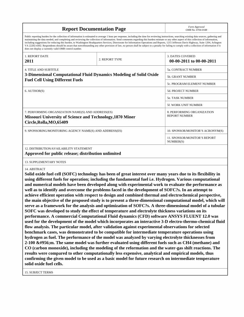
14. ABSTRACT Solid oxide fuel cell (SOFC) technology has been of great interest over many years due to its flexibility inusing different fuels for operation; including the fundamental fuel i.e. Hydrogen. Various computationaland numerical models have been developed along with experimental work to evaluate the performance aswell as to identify and overcome the problems faced in the development of SOFC?s. In an attempt toachieve efficient operation with respect to design and combined thermal and electrochemical perspective,the main objective of the proposed study is to present a three-dimensional computational model, which willserve as a framework for the analysis and optimization of SOFC?s. A three-dimensional model of a tubularSOFC was developed to study the effect of temperature and electrolyte thickness variations on itsperformance. A commercial Computational Fluid dynamics (CFD) software ANSYS FLUENT 12.0 wasused for the development of the model which incorporates an interactive 3-D electro-thermo-chemical fluidflow analysis. The particular model, after validation against experimental observations for selectedbenchmark cases, was demonstrated to be compatible for intermediate temperature operations usinghydrogen as fuel. The performance of the model was analyzed by varying electrolyte thicknesses from2-100 μm. The same model was further evaluated using different fuels such as CH4 (methane) andCO (carbon monoxide), including the modeling of the reformation and the water-gas shift reactions. Theresults were compared to other computationally less expensive, analytical and empirical models, thusconfirming the given model to be used as a basic model for future research on intermediate temperaturesolid oxide fuel cells.

15. SUBJECT TERMS

16. SECURITY CLASSIFICATION OF: 17. LIMITATION OF ABSTRACT Same as

Report (SAR)

18. NUMBEROF PAGES

83

19a. NAME OFRESPONSIBLE PERSON

a. REPORT unclassified

b. ABSTRACT unclassified

c. THIS PAGE unclassified

Standard Form 298 (Rev. 8-98) Prescribed by ANSI Std Z39-18

2011

Sachin Laxman Puthran

All Rights Reserved

iii

ABSTRACT

Solid oxide fuel cell (SOFC) technology has been of great interest over many years

due to its flexibility in using different fuels for operation; including the fundamental fuel

i.e. Hydrogen. Various computational and numerical models have been developed along

with experimental work to evaluate the performance as well as to identify and overcome

the problems faced in the development of SOFC’s. In an attempt to achieve efficient

operation with respect to design and combined thermal and electrochemical perspective,

the main objective of the proposed study is to present a three-dimensional computational

model, which will serve as a framework for the analysis and optimization of SOFC’s.

A three-dimensional model of a tubular SOFC was developed to study the effect of

temperature and electrolyte thickness variations on its performance. A commercial

Computational Fluid dynamics (CFD) software ANSYS FLUENT 12.0 was used for the

development of the model which incorporates an interactive 3-D electro-thermo-chemical

fluid flow analysis. The particular model, after validation against experimental

observations for selected benchmark cases, was demonstrated to be compatible for

intermediate temperature operations using hydrogen as fuel. The performance of the

model was analyzed by varying electrolyte thicknesses from 2-100 μm. The same model

was further evaluated using different fuels such as CH4 (methane) and CO (carbon

monoxide), including the modeling of the reformation and the water-gas shift reactions.

The results were compared to other computationally less expensive, analytical and

empirical models, thus confirming the given model to be used as a basic model for future

research on intermediate temperature solid oxide fuel cells.

iv

ACKNOWLEDGMENTS

I would like to thank my advisor Dr. Umit O. Koylu for his guidance,

encouragement and financial support throughout this research work. I am also thankful to

my co-advisors and also graduate committee members, Dr. Serhat Hosder and Dr. Fatih

Dogan for extending their help in relevant topics needed for the research and also for

serving in the committee, taking time out of their busy schedules. I am grateful to the

Energy Research and Development Center at Missouri University of Science and

Technology and the Air Force Research Laboratory (AFRL) for funding my research. I am

also grateful to all the faculty members of the department who have contributed in my

learning of the required skills to finish this work.

I would like to thank all my friends for being with me always in tough times so far

away from home. And last, but not the least, I would like to express my gratitude to my

parents, my sister and my entire family for their love, affection and support.

v

TABLE OF CONTENTS

Page

ABSTRACT.................................................................................................. iii

ACKNOWLEDGMENTS........................................................................................ iv

LIST OF ILLUSTRATIONS.................................................................................... vii

LIST OF TABLES.................................................................................................... viii

NOMENCLATURE.................................................................................................. ix

SECTION

1. INTRODUCTION........................................................................................ 1

1.1. FUEL CELL THEORY........................................................................ 1

1.2. SOLID OXIDE FUEL CELL THEORY............................................. 5

1.3. OBJECTIVES...................................................................................... 7

2. LITERATURE REVIEW............................................................................ 9

3. SOFC MODELING..................................................................................... 15

3.1. GEOMETRIC MODEL............................................................................... 15

3.2. COMPUTATIONAL MODEL........................................................... 19

3.2.1. Computational Model Theory.................................................... 19

3.2.2. Case Setup.................................................................................. 25

4. MODEL VALIDATION............................................................................. 29

4.1. BOUNDARY CONDITION SETUP................................................... 30

4.2. RESULTS AND ANALYSIS.............................................................. 31

5. PARAMETRIC ANALYSIS....................................................................... 35

5.1. TEMEPRATURE DEPENDENCE & EFFECT OF POROSITY....... 35

5.2. EFFECT OF ELECTROLYTE THICKNESS..................................... 41

5.3. ANALYSIS USING DIFFERENT FUELS......................................... 44

5.3.1. CO Electrochemistry Model...................................................... 44

vi

5.3.2. Modeling the reformation and Water-gas shift reaction using CH4 as fuel............................................................................ 46

6. CONCLUSIONS AND FUTURE WORK.................................................. 54

6.1. CONCLUSIONS AND DISCUSSIONS............................................. 54

6.2. FUTURE WORK SUGGESTIONS..................................................... 55

APPENDIX: FLUENT TUTORIAL FOR SETTING UP THE TUBULAR SOFC MODEL …………………………………………………………….. 57

BIBLIOGRAPHY..................................................................................................... 70

VITA......................................................................................................................... 73

vii

LIST OF ILLUSTRATIONS

Figure Page

1.1. General architecture of a fuel cell................................................................... 2

1.2. Planar and tubular SOFC configuration........................................................... 5

1.3. Working of SOFC.............................................................................................. 6

3.1. Cross section of tubular SOFC model.............................................................. 17

3.2. Figure showing mesh structure for the model.................................................... 18

4.1. Comparison plot with experimental results from Barzi et al............................. 32

4.2. Plot of power density vs. current density for present model.............................. 33

5.1. Plot of total voltage vs. average current density for different cases with variation in temperature (T) and cathode porosity (p)....................................... 36

5.2. Power density plotted against average current density for temperature dependence study........................................................................... 37

5.3. Contour plots of current density, voltage & temperature distribution............... 38

5.4. Plot of H2 mole fraction over length of cell for all 5 cases................................ 40

5.5. Plot of H2O mole fraction over length of cell for all 5 cases............................. 40

5.6. Plots to study the electrolyte thickness variation effects.................................... 42

5.7.Contour plots of current density, voltage and temperature for CO electrochemistry model..................................................................................... 45

5.8.Contour plots of the distribution of fuel species in the flow channel and on electrolyte surface........................................................................................... 49

5.9. Plot showing distribution of H2O along length of cell....................................... 51

5.10. Contour plots for kinetic rates of reaction........................................................ 52

viii

LIST OF TABLES

Table Page

1.1.Types of fuel cells.......................................................................................................... 4

3.1. Geometrical properties of the model in study.................................................... 16

3.2. Material specifications for model....................................................................... 26

3.3. Electrical properties of the SOFC model........................................................... 27

4.1. Cell zone conditions and boundary conditions applied to the present model.... 30

5.1. Comparison of results for the model with Stiller et al....................................... 48

ix

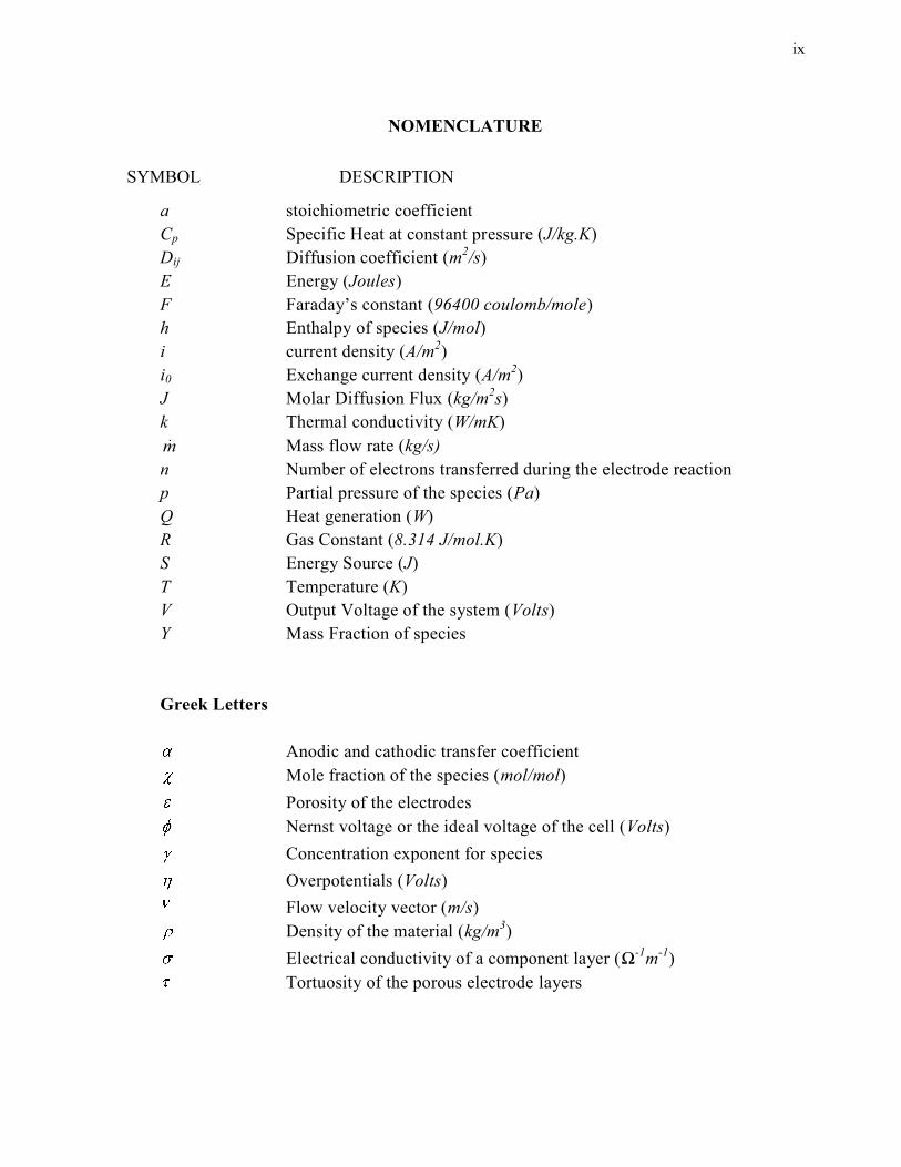
NOMENCLATURE

SYMBOL DESCRIPTION

a stoichiometric coefficient Cp Specific Heat at constant pressure (J/kg.K) Dij Diffusion coefficient (m2/s) E Energy (Joules) F Faraday’s constant (96400 coulomb/mole) h Enthalpy of species (J/mol) i current density (A/m2) i0 Exchange current density (A/m2) J Molar Diffusion Flux (kg/m2s) k Thermal conductivity (W/mK) m Mass flow rate (kg/s) n Number of electrons transferred during the electrode reaction p Partial pressure of the species (Pa) Q Heat generation (W) R Gas Constant (8.314 J/mol.K) S Energy Source (J) T Temperature (K) V Output Voltage of the system (Volts) Y Mass Fraction of species Greek Letters

Anodic and cathodic transfer coefficient Mole fraction of the species (mol/mol) Porosity of the electrodes Nernst voltage or the ideal voltage of the cell (Volts) Concentration exponent for species Overpotentials (Volts) Flow velocity vector (m/s) Density of the material (kg/m3) Electrical conductivity of a component layer (Ω-1m-1) Tortuosity of the porous electrode layers

x

Superscripts and Subscripts 0 Denotes standard or reference state a Anodic act related to activation losses c Cathodic cell Referring to cell properties eff Effective property elec Referring to electrolyte h heat source i Referring to species i ideal Ideal property j Referring to species j jump voltage Jump condition ohmic Related to ohmic losses ref Referring to the reference state

1. INTRODUCTION

In recent years, energy has become the most important and challenging aspect of

our existence. Tremendous interest and effort have been put into developing new and

improved methods of energy generation. Power generation using electrical energy has

been of prime importance due to its extensive applications. Various resources, both

renewable and non-renewable were introduced into the power industry in the process.

Emphasis has been given to alternative sources of energy conversion due to the limitations

of the conventional sources. This need gave rise to the concept of fuel cells as an

alternative source of energy. Fuel cells coupled with other renewable energy sources like

wind, solar etc. can prove to be very useful and clean source of power generation.

1.1. FUEL CELL THEORY

The origin of fuel cell dates back to the late 19th century, when Sir William Grove

found out that it was possible to generate electricity by reversing the electrolysis of water

[1]. A fuel cell is an electrochemical device consisting of a minimum of two electrodes

separated by an electrolyte. As stated in O’Hayre et al. [2], it is like a factory, a shell,

which converts the chemical energy stored in the fuel into electrical energy. It produces

electricity directly from the chemical reactions by harnessing the electrons as they move

from high-energy reactant bonds to low-energy product bonds. The electrolyte being used

is an ion conducting material, either liquid or solid phase, which separates the fuel and the

oxidizer so that the electron transfer needed to complete the bonding reconfiguration

occurs over an extended area. The electrolyte used in the fuel cell, plays a very important

2

role in any fuel cell operation, as it has to be capable of permitting only the appropriate

ions through it to generate electricity efficiently. The electrons thus released will move

from the fuel species to the oxidant species through an external circuit. This movement of

the electrons generates electrical current, which can be used for various applications.

Figure 1.1 shows the general architecture of a fuel cell, stating the arrangement of the

zones.

Figure 1.1 General architecture of a fuel cell

The general electrochemical reactions occurring in a basic hydrogen-oxygen fuel

cell are shown in the equations 1.1-1 and 1.1-2.

22 2 2H O H O e (Anodic Reaction) (1.1-1)

21 22

O e O (Cathodic Reaction) (1.1-2)

Load

2e-

2e-

3

Fuel cells exhibit a potential for highly reliable and long lasting systems with very

low emissions because of their capability to directly produce electricity from the chemical

energy, without involving any moving parts. They are a clean and almost entirely non-

polluting energy source. Also, the elimination of moving parts makes them vibration–free

and the associated noise-pollution is also eliminated. The working of fuel cells make

them share common characteristics with the conventional combustion engines and

primary batteries, combining various advantages of both the types of energy conversion

devices. The efficiency obtained by this process is also higher (40%-60%) compared to

the conventional devices [3]. The applications of fuel cells are usually based on the type

of the fuel cell being used.

Various types of fuel cells have been put to use and are in different stages of their

development. The 5 major types of fuel cells in practice are listed below:

Polymer Electrolyte Membrane Fuel Cell (PEMFC)

Alkaline Fuel cell (AFC)

Phosphoric Acid Fuel Cell (PAFC)

Molten Carbonate Fuel Cell (MCFC)

Solid Oxide Fuel Cell (SOFC)

This classification in fuel cells broadly depends on the type of the electrolyte being used.

The type of the electrolyte lays influence over the other thermo-physical properties such

as the operating temperature of the cell and the material properties of the other cell

components. A large variation can be found in the operating temperatures of these fuel

cell types, ranging approximately from 80 oC to 1000 oC. Usually, in low temperature fuel

cells, the fuel used is pure hydrogen wherein all the fuel is required to be converted to

4

hydrogen before being fed to the low temperature fuel cells. Some high temperature fuel

cells possess this advantage over the low temperature one’s that CO or other hydrocarbon

fuels can be converted to hydrogen internally in the fuel cells or can even be directly

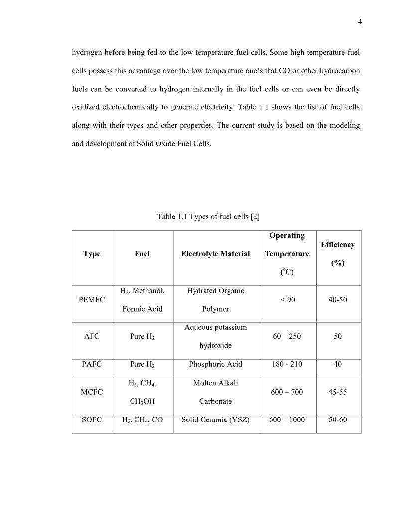
oxidized electrochemically to generate electricity. Table 1.1 shows the list of fuel cells

along with their types and other properties. The current study is based on the modeling

and development of Solid Oxide Fuel Cells.

Table 1.1 Types of fuel cells [2]

Type Fuel Electrolyte Material

Operating

Temperature

(oC)

Efficiency

(%)

PEMFC H2, Methanol,

Formic Acid

Hydrated Organic

Polymer < 90 40-50

AFC Pure H2 Aqueous potassium

hydroxide 60 – 250 50

PAFC Pure H2 Phosphoric Acid 180 - 210 40

MCFC H2, CH4,

CH3OH

Molten Alkali

Carbonate 600 – 700 45-55

SOFC H2, CH4, CO Solid Ceramic (YSZ) 600 – 1000 50-60

5

1.2. SOLID OXIDE FUEL CELL THEORY

Solid Oxide Fuel Cells (SOFC) in particular are considered as promising energy

conversion devices due to a number of potential benefits, including high energy

efficiency, lower pollutant emissions, possibility of using different fuels and combined

heat and power generation applications. SOFC’s operate at high temperatures in the range

of about 600 oC-1000 oC [2]. This high temperature operation of SOFC’s provide multiple

co-generation possibilities such as internal reforming of hydrocarbon fuels to generate

hydrogen, which is not possible in other types of fuel cells. It also facilitates production of

high quality steam, which can be efficiently used for other applications. A number of

different designs have been tested in need of optimizing the performance of these cells.

The common geometries used are shown in Figure 1.2.

Figure 1.2 Planar and tubular SOFC configuration

Planar Model Tubular model

Anode

cathode

Flow channels

cathode

Anode

Electrolyte

Fuel flow channels

Air flow channels

6

Two basic geometries of SOFC’s have been studied quite actively in the relevant

literature viz. the planar SOFC design and the tubular design. Both types have their own

advantages and disadvantages and have been discussed in detail in the cited literature.

Figure 1.2 shows the general configuration of the planar and tubular geometry of SOFC’s.

The working of a Solid Oxide fuel cell is different to that of other types of fuel

cells. The electrolyte material is a ceramic solid which is a very good ion conductor at

elevated temperatures. In SOFC operation, the oxygen ions travel through the electrolyte

from the cathode to the anode, and reacts with the hydrogen molecules at the Triple phase

boundary (TPB) on the anode. This electrochemical reaction produces H2O and releases

electrons in the anode. These electrons travel through the anode and the current collectors

and through the external circuit to the cathode to react with the oxygen molecules. This

phenomenon generates the electrical current due to the potential developed. The working

of the Soild Oxide Fuel cell is well explained in the Figure 1.3.

Figure 1.3. Working of SOFC

22 2 2H O H O e

2

1 22

O e O

H2

H2O

O2-

2e-

Cat

ho

de

An

od

e

Oxidizer Fuel

7

1.3. OBJECTIVE

Despite the advantages, there have been certain limitations on the applications of

SOFC’s, where relatively high operating temperatures are of great concern. It becomes

difficult and expensive to acquire materials withstanding such high temperatures. Based

on these concerns, efforts are being made to reduce the temperatures involved by

developing intermediate temperature SOFC’s. This concept is gaining importance to

enhance the long term stability prospects of Solid Oxide Fuel cells. Efforts are being made

by developing experimental, mathematical and computational models and prototypes to

achieve optimum operating conditions for specific target area applications of SOFC’s.

This calls for a need of fundamental and detailed understanding of the design, transport

and electrochemical kinetics involved in the SOFC systems. Mathematical and

computational models can prove to be extremely valuable tools for the design and analysis

compared to the much expensive experimental evaluation techniques. However a

combination of these techniques can be used as a comparably accurate method for the

characterization and validation of SOFC systems.

A three-dimensional computational fluid dynamics (CFD) model of a Solid Oxide

fuel cell was developed in the work mentioned in this thesis. A single cell cathode-

supported, tubular geometry was considered for the design, which is one of the common

and most used designs in the fuel cell industry. This model is used to carry out analysis,

by varying parameters involved in the operation to optimize the performance of the SOFC

for the given set of conditions and design. This model serves as a framework or guideline

for setting up successful experimental work for the analysis and optimization of SOFC’s.

A commercial CFD software, ANSYS FLUENT 12.0 is used for the analysis, which

8

incorporates a complete electro-thermo-chemical fluid flow analysis. A computational

evaluation of this model with the varying parameters will help in the optimization study of

the currently installed models based on the current density and the thermal distribution

fields generated within a single cell. The results are compared against relevant benchmark

SOFC models existing in the literature.

9

2. LITERATURE REVIEW

The objective of this work is to develop a base model for a tubular Solid Oxide

Fuel Cell which can be considered to resemble the actual practical model of a SOFC,

taking into account all the conservation principles. As described earlier, a computational

model of the desired design will enable a comparatively detailed analysis of the model

under consideration. A 3-dimensional model will consider the physics involved in the

model in all the significant directions, thus providing us with a detailed analysis of the

SOFC model.

Solid Oxide fuel cells have been a subject of extensive study since the 1960’s as a

promising prospective option for clean energy generation. The first successful

demonstration of a Solid Oxide fuel cell was performed in 1962 [1]. Since then, a lot of

experimental work has been performed along-with the various numerical and

mathematical models to predict the behavior of Solid Oxide Fuel cells to varying

conditions. Westinghouse started the concept of long tubular cells (inside air, outside

fuel), electrically interconnected by oxides and metallic conductors and accumulated

together in tube bundles in 1978 [2, 4]. This design lead to the installation of the first 5

kW SOFC Generator consisting of 324 single cells in 1986 [4-5]. After 12 years, in 1998,

a 100 kW SOFC power generator was installed in Netherlands, consisting of 1152 tubular

cells[4]. Research work on different SOFC designs has been on its peak over all these

years. Majority of the research work are focused on the optimization of the design and the

materials used in Solid Oxide fuel cells.

Mathematical and Numerical models along with the experimental analysis have

proved to be an extremely useful tool over the years. A mathematical model for

10

simulation of planar Solid Oxide fuel cells was introduced by Karoliussen and

Nisancioglu et al. [6] and by Achenbach et al. in 1994 [7]. Both the studies focused on the

effect of different flow structures on the performance of planar SOFC’s. But the equations

used in these modeling approaches did not account for the heat transfer or conduction

through the interconnects [7]. The first mathematical model for a Tubular SOFC was

developed by Bessette et al. in 1995 [8-9] which accounted for the electrochemical and

thermal factors of the tubular cell resembling the Westinghouse design. The data required

for the analysis were obtained from fundamental equations or were independently

measured to avoid any discrepancies in the evaluation.

Due to the extremely high operating temperatures related to Solid Oxide fuel cells,

the materials used in the construction of a cell play a very important role. This has given

rise to a lot of active research work in the micro-modeling of SOFC’s, which is associated

with the micro-level properties of the SOFC materials such as the pore structures, thermal

and electrical conductivities, active area etc. for the electrochemical reactions to take

place.In 1998, Costamagna et al. [10] developed a micro-model of SOFC electrodes

having LSM/YSZ cathodes and Ni/YSZ anodes which helped in understanding a

relationship between the electrochemical properties of the materials used, related to the

structural parameters. A one-dimensional anode micro-model including the study of the

transport of electrons, ions and molecules through the electrode micro-structure were

studied by Chan and Xia et al. [11]. Recently, in 2010, Ding et al. [12] studied the anode

supported SOFC’s in more detail using experimental models for analyzing the

performance of the Solid Oxide fuel cells for varying thicknesses. A GDC (Gadolinium

doped ceria) electrolyte was used for the study and it was observed that lower electrolyte

11

thickness was favorable but further reduction of thickness below 5 μm gave rise to

electron flux through the electrolyte film, thus degrading the electrical performance of the

anode-supported SOFC.

Another advancement in the field of SOFC’s included the introduction of the

concept of single chamber SOFC’s. This concept was considered very promising for

reducing the complexity of the SOFC operations. The single chamber concept simplified

the design prospects of SOFC’s considerably, where the fuel and the oxidizer were

premixed and then fed into the fuel cell channel. In 2005, Chung et al.[13] developed a

computational model of a single chamber SOFC, modeling the multi-physical phenomena

(ionic conduction, fluid dynamics and gas diffusion). The best performance for the micro-

single chamber design was observed when the inflow direction was kept perpendicular to

the electrode axis. Akhtar et al. [14] developed a 3-dimensional numerical model for a

single chamber design in 2009, which used nitrogen diluted hydrogen/oxygen mixture to

predict the hydrodynamic and electrochemical performance of the SOFC single cell. Also

the porosity of the electrodes played an important role in the electrochemical performance

of the cell. Single chamber designs are considered as a promising concept, but their

applications are still far-fetched due to the various problems involved with pre-mixing of

the fuel and the oxidizer which makes it difficult to control the various reactions that

could be initiated, rendering the process out of control.

The basic dual-chambered geometries are the most researched topics recently,

which have been already installed and are put to use. Optimization of these basic designs

can be considered as more important currently with an application point of view. A lot of

researchers have laid focus on modeling of the planar single cells as well as stack designs.

12

In 2001, Yakabe et al. [15] developed a 3-D mathematical model for a planar single cell

SOFC. A finite volume method was employed to solve the conservation equations, taking

into account the internal and external reforming reactions, the water shift reaction and the

diffusion of the species. It was observed that the reformation reaction induced a steep drop

in the temperature of the fuel near the inlet developing stresses, and the co-flow pattern

was found to be advantageous to mitigate the steep temperature gradient and to reduce the

internal stresses. Even Recknagle et al. [16] (2002) evaluated the planar SOFC design for

different flow patterns and found out that the co-flow design had the most uniform

temperature distribution and the smallest thermal gradients, thus providing thermo-

structural advantages to the model. Murthy and Fedorov [17], in 2003, applied different

computational methods to quantify the effect of radiation heat transfer in the SOFC

monolith design, which is neglected in most of the modeling cases. They concluded that

the radiation heat transfer effect were significant and should be considered for accurate

predictions of the temperature distribution in the cell and the cell voltage. Other literature

on modeling and optimization of planar SOFC cells involved a numerical model by Lin

and Beale [18] in 2003 and 3-D thermo-fluid modeling of anode-supported planar SOFC

by Zuopeng Qu et al. [19] which again emphasized on the importance of all the modes of

heat transfer in performance prediction of the planar SOFC’s.

Although the fabrication and arrangements of planar cells are comparatively

easier, tubular cells exhibit better stability against mechanical and thermal stresses and

they also provide better sealing between the air and the fuel flow channels [2]. Some

significant research work in development of tubular SOFC’s are cited. Fang et al. [20]

developed a 1-dimensional transient model of a tubular SOFC considering the

13

thermoelectric properties by recording the dynamic behavior of the electrical

characteristics and temperature under variable load conditions. Three transient cases viz.

start-up, load resistance decrease and air-flow decrease were employed to capture the

dynamic behavior of SOFC stacks. In 2004, Campanari and Iora [21] developed a finite

volume model of a tubular SOFC single cell and carried out a sensitivity analysis,

considering all the thermal and electrochemical analysis including the heat exchange

processes and the internal reforming cases. This paper is cited in most of the research

work on tubular SOFC’s. Another useful contribution in the tubular SOFC modeling

literature is the model described by Suwanwarangkul et al. [22] (2005). A 2-dimensional

mechanistic model of a cathode supported tubular SOFC was developed to account for the

thermal and electrochemical properties of the SOFC. In 2007, the same model was used to

predict the effect of the composition of the biomass derived synthesis gas fuels on the cell

performance and behavior [23]. A transient numerical analysis was carried out by Mollayi

Barzi [24] in 2009, combining the heat and mass transport effects, which gave more

realistic results compared to the 1-dimensional and lumped models due to the

consideration of the state variable gradients in the radial direction. It was observed that

82% of the electrical parameter variations take place immediately after the load change

and the remaining 18% variations take a very long time to reach a steady state. Stiller et

al. [25] developed steady state models for both planar and tubular cells fueled by partially

pre-reformed methane to study the hybrid cycle performance of SOFC stacks. It was

observed that the air pre-heating internally in case of tubular SOFC was advantageous in

improving the effectiveness of the GT cycle. Hybrid system efficiencies of above 65%

were achieved using both the planar and tubular geometries.

14

As mentioned previously, the modeling approach mentioned in this work is based

on the 3-dimensional computational analysis of SOFC’s using commercial computational

softwares. These computational software packages have contributed in the SOFC

modeling studies and are also proven to be efficient in saving time required for the

analysis. Several commercial CFD software packages such as FLUENT, COMSOL

MULTIPHYSICS, CFX, STAR-CD, CFD-ACE etc. have been used for the modeling

purposes. The single chamber model by Akhtar et al.[14] mentioned earlier used

COMSOL MULTIPHYSICS for the 3-D model, accounting for the hydrodynamic and

electrochemical performance of the model. In 2003, Autissier et al. [26] developed a 3-

dimensional simulation tool using FLUENT, which also accounted for the radiative heat

transfer in the single cell. Other literature work using the FLUENT simulation tool for

SOFC modeling include the CFD model developed by Pasaogullari and Wang [27]

making use of the UDF (User defined function) developed by FLUENT, taking care of the

electrochemical reactions of the SOFC. In 2010, Sleiti et al. [28] analyzed the

performance of tubular SOFC at reduced temperatures and cathode porosity using the

FLUENT 6.3 SOFC UDF; the model developed resembled the Westinghouse design and

is also similar to the model described in the present research mentioned in this thesis. The

model was found to demonstrate the capability of SOFC’s to operate at intermediate

temperatures given that the transport properties of the electrodes and the electrolyte were

kept the same. The model mentioned in the current thesis also makes use of the FLUENT

12.0 SOFC UDF to model the electrochemical reactions involved in the SOFC operation,

integrated with the other conservation equations.

15

3. SOFC MODELING

The grid for the three-dimensional SOFC model was generated using GAMBIT

2.3.16. The tubular design was made to resemble the Westinghouse concept, which is

already been installed, as mentioned in Section 2. This tubular design was used to set-up a

base case using a commercial computational analysis software viz. ANSYS FLUENT,

which takes into account all the complex electro-thermo-chemical properties by simulating

the complex processes involved in the SOFC operation. FLUENT makes use of

computational methods to solve the conservation equations which take care of the

parameters involved and help us simulate a near-actual case, thus helping in optimization

study of the SOFC operation using different perspectives. The modeling strategy and

procedure is described in detail in the following sections.

3.1. GEOMETRIC MODEL

As mentioned earlier, a geometric modeling and meshing software viz. GAMBIT

(version 2.3.16) was used for developing the model. GAMBIT is considered as a pre-

processor for FLUENT, since the zone definitions and the meshing strategy can be easily

imported into the FLUENT solver, for further analysis.

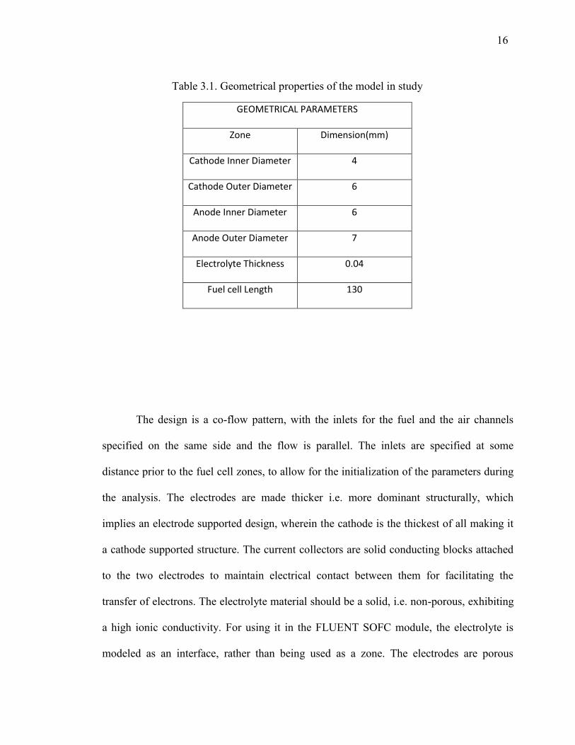
The tubular geometry described in the work is a 130 mm long concentric tube,

with layers of the flow channels and the electrodes. The inner tube is the air electrode

(cathode) and the fuel flows through the outermost tube adjacent to the fuel electrode

(anode). The electrolyte is sandwiched between the two electrodes. Table 3.1 shows the

important zones and the dimensions of the model being developed.

16

Table 3.1. Geometrical properties of the model in study

GEOMETRICAL PARAMETERS

Zone Dimension(mm)

Cathode Inner Diameter 4

Cathode Outer Diameter 6

Anode Inner Diameter 6

Anode Outer Diameter 7

Electrolyte Thickness 0.04

Fuel cell Length 130

The design is a co-flow pattern, with the inlets for the fuel and the air channels

specified on the same side and the flow is parallel. The inlets are specified at some

distance prior to the fuel cell zones, to allow for the initialization of the parameters during

the analysis. The electrodes are made thicker i.e. more dominant structurally, which

implies an electrode supported design, wherein the cathode is the thickest of all making it

a cathode supported structure. The current collectors are solid conducting blocks attached

to the two electrodes to maintain electrical contact between them for facilitating the

transfer of electrons. The electrolyte material should be a solid, i.e. non-porous, exhibiting

a high ionic conductivity. For using it in the FLUENT SOFC module, the electrolyte is

modeled as an interface, rather than being used as a zone. The electrodes are porous

17

ceramic solids while the interlayers are modeled as a pair of wall and wall shadow faces.

These surfaces are modeled with species and energy sources and sinks due to

electrochemical reactions added to adjacent computational cells. Figure 3.1 shows the

cross section of the GAMBIT model of the tubular design. The different zones are labeled

to show the architecture of the model.

Figure 3.1. Cross section of tubular SOFC model

The FLUENT solver uses the finite volume method to solve the conservation

equations, which makes use of cells as control volumes in the flow field. A hexahedral

mesh is generated for the entire volume, where the cells in the zones are hexahedral and

face cells are quadrilateral. There are a total of 79680 cells for the entire volume of the

Fuel flow

channel

Anode

Cathode

Air flow channel

Current collector

Electrolyte

Interface

Current collector

18

model. The maximum aspect ratio is limited to 20. O-structured mesh is generated on the

concentric faces of the model, giving a good mesh quality (skewness). The mesh structure

of the model is shown in the Figure 3.2.

Figure 3.2. Figure showing mesh structure for the model

This model was exported to the FLUENT solver, for further analysis, where the

complex conservation equations are solved based on certain different parameters involved.

The next section will describe the computational modeling of the prototype.

19

3.2. COMPUTATIONAL MODEL

The model described in this research work uses ANSYS FLUENT SOFC module

(version 12.0). The details of the modeling strategy are explained in the fuel cells module

manual by FLUENT [29]. The 3-dimensional tubular SOFC model employs the CFD

modeling software to numerically solve the set of partial differential equations involved in

the SOFC modeling theory. These partial differential equations describe the heat and mass

transfer through the flow channels and the electrodes, the fuel flow and the chemical and

electrochemical reactions occurring in the SOFC’s. A User Defined Function is employed

to model the electrochemical reactions particularly, since they involve some electrical

principles which have to be defined in UDF’s. The UDF solves for the potential

developed in the operation, the current distribution and the different overvoltages (losses)

in the fuel cell operation. The electrical model accounts for the potential field in the

conductive layers of the cell. The two electrodes in the model are connected using the

potential jump feature in the UDF’s, for calculating the potential. The mass diffusion

model used in the solver, corrects the effect of porosity and tortuosity in the porous media

using the multi-component diffusion model.

3.2.1. Computational Model Theory. Computational fluid dynamics modeling of

Solid oxide fuel cells requires modeling of the following listed phenomena in the cell.

Fluid Flow: This involves the flow of fuel and air in the flow channels i.e. in the

porous and the non-porous media, which can be predicted by solving the conservation

of momentum principle.

Mass Transfer: The mass conservation equation and the species conservation equation

are solved to account for the diffusion of fuel and air in the porous electrodes.

20

Heat Transfer: This accounts for the conduction of heat in the solid regions of the cell

and the convective heat transfer in the electrodes and through the layers, by solving the

energy conservation equation.

Electrochemical Reactions: The electrochemical reactions occurring at the electrodes

are accounted for, with the release of ions and electrons.

Current and potential field transport: This phenomenon accounts for the transfer of

ions and electrons and the calculation of the cell potential and the current generated.

These phenomena are modeled by solving the above mentioned conservation

equations by adopting the finite volume method, using the implicit discretization scheme.

The modeling assumptions used for solving these equations are as listed below [29]:

The flow is considered as incompressible and laminar, due to the low velocities and

low utilization factors

Steady state operation

All components are assumed to have similar thermal expansions

Radiation heat transfer effects are neglected (single cell model)

Reactions are assumed to take place in a single step

Charge transfer reaction is considered as the rate limiting reaction

The conservation of momentum principle to model the flow of fuel and air through

different zones in the fuel cell operation is given by Equation 3.2.1-1

21

,. .i i s iv vy J St

(3.2.1-1)

For the porous electrodes, an effective binary diffusion coefficient is calculated,

accounting for the porosity and the tortuosity of the electrode structures. Equation 3.2.1-2

shows the expression for the effective binary diffusion coefficient.

,ij eff ijD D (3.2.1-2)

The conservation of charge principle applied to the conductive regions states that

. 0i (3.2.1-3)

Where i is, i (3.2.1-4)

The Laplace equation is used as the governing principle for solving the species

conservation equation,

0 (3.2.1-5)

The oxygen in the air flow-channel gets reduced to O2- ions, which diffuses through the

porous cathode and the electrolyte to react with the hydrogen atoms at the TPB on the

anode side. The electrochemical reaction results in release of electrons which pass through

the external circuit connected together by the current collectors. The transfer of electrons

generates a current through the circuit, developing a potential difference across the two

electrodes. The output voltage of the cell is calculated using the Nernst Equation

[29](Equation 3.2.1-6) while the current density and the activation overpotentials are

calculated using the Butler-Volmer relations [29](Equation 3.2.1-9).

22

At equilibrium, the reversible cell voltage (Nernst Voltage) is given by Equation

3.2.1-6,

2 2

2

12

0 ln4

H Oideal

H O

p pRTF p

(3.2.1-6)

The actual cell potential is lower than the Nernst voltage by reduction due to activation,

Ohmic losses due to resistivity of the electrolyte, and a linearized for voltage reduction due

to activation,

cell jump (3.2.1-7)

Where,

, ,jump ideal ele act a act c (3.2.1-8)

The current density on the interface can be calculated using the Butler-Volmer equation

where the reaction rates are written in terms of the exchange current density.

, ,

0,

a act a c act cn F n FRT RT

effi i e e (3.2.1-9)

Where, 0, 0,.

j

jeff ref

j ref

i i (3.2.1-10)

More specifically, the effective exchange current density can be calculated for the anode

side and the cathode side; for the anode side:

23

2 2

2 2

2 2

0, 0, ,

H H O

H H Oanode anodeeff ref

H ref H O ref

i i (3.2.1-11)

and for the cathode side,

2

2

2

0, 0,,

O

Ocathode cathodeeff ref

O ref

i i (3.2.1-12)

The Butler-Volmer equation can be solved using the Newton’s method after the initial

input values for the model are provided. The activation overpotentials for the cathode and

the anode are calculated using this equation.

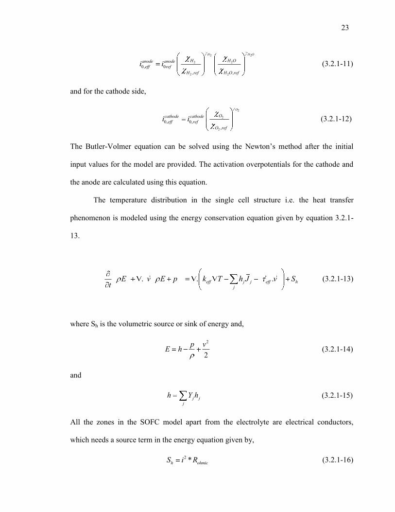
The temperature distribution in the single cell structure i.e. the heat transfer

phenomenon is modeled using the energy conservation equation given by equation 3.2.1-

13.

. . .eff j j eff hj

E v E p k T h J v St

(3.2.1-13)

where Sh is the volumetric source or sink of energy and,

2

2p vE h (3.2.1-14)

and

j jj

h Y h (3.2.1-15)

All the zones in the SOFC model apart from the electrolyte are electrical conductors,

which needs a source term in the energy equation given by,

2 *h ohmicS i R (3.2.1-16)

24

Equation 3.2.1-16 accounts for the ohmic heating in the cell zones due to the electrical

conduction, but the model also needs to take into account the heat generated or lost due to

the electrochemical reactions and due to the overpotentials (losses) in the fuel cell

operation. The enthalpy flux terms are introduced into the energy equation to take care of

the electrochemistry, Equation 3.2.1-17 and Equation 3.2.1-18 show a general energy

balance for hydrogen reaction and the enthalpy of formation for the same, respectively.

2 2 2

" " " "H O H OQ h h h i V (3.2.1-17)

2 2 0

ref

T

H H pT

h m C dT h (3.2.1-18)

The last term in Equation 3.2.1-17 is the work done by the system which is

calculated as a product of the local voltage jump and the local current density. The effects

of all overpotentials are taken into account by the introduction of the work term for each

electrode into the energy equation.

The ohmic resistance in the conducting regions is calculated as:

.ohmic i R (3.2.1-19)

The electrochemical reactions are modeled by calculating the rate of species

production and destruction, thus calculating the dependence of the concentration of species

on the current-voltage characteristics of the cell,

aiSnF

(3.2.1-20)

25

By convention the current density i is considered positive when it flows from

electrode into the electrolyte solution, i.e. the current densities are positive at the anodes

and negative at the cathodes. Equation 3.2.1-20 can be used with the conventions to

quantify the source terms for the calculations, depending on the electrochemistry involved.

3.2.2. Case Setup. The flow is defined as a viscous laminar flow through both

tubes. The fuel and air flow rates are 2.5x10-7 kg/s and 1.35x10-5 kg/s respectively [2, 28].

The fuel flows through the outer tube diffusing through the porous anode to reach the

Triple Phase Boundary (TPB). The air flows through the inner tube at the given flow rate.

The inlet temperature for fuel and air is considered to be 973 K to facilitate for faster

reaction rates, increasing the effective time of the SOFC operation. Materials are specified

for each component using the available materials and also defining new materials in the

FLUENT database. The material properties for the components are listed in Table 3.2.

The SOFC Module developed by FLUENT takes the material properties which are

defined by the user, along with the electrical parameters which can also be specified by

the user as per the required case. The electrical properties used for this case are shown in

Table 3.3. Since, not all the electrical and electrochemical parameters needed for the

specifications are mentioned in the literature, some of these values have to be calculated

approximations, used to try and match the results to the referred case. The values

mentioned in Table 3.2. and Table 3.3. were extracted from the FLUENT UDF Manual

examples.[29]

26

Table 3.2. Material specifications for model

MATERIAL PROPERTIES

Property Zones

Anode Cathode Current

Collector Electrolyte

Material Ni-Doped YSZ LSM Ferritic

Chromium steel YSZ

Density(ρ) kg/m3 3030 4375 8900 5371

Thermal

conductivity (k)

W/mK

595.1 Temperature

Dependent 446 585.2

Specific heat (cp)

J/kg K 6.23 1.15 72 2.2

Porosity (Є) % 30 30 Impermeable Impermeable

Tortuosity (τ) 3 3 - -

27

Table 3.3. Electrical properties in the SOFC model

ELECTRICAL PROPERTIES

Property Value

Total system current (Amp) 8

Electrolyte resistivity (ohm - m) 0.1

Current under relaxation factor 0.3

Anode exchange current density (Amps) 1.00e+20

Cathode exchange current density (Amps) 512

- Anodic transfer coefficient 0.5

- Cathodic transfer coefficient 0.5

- Anode Conductivity (1/ohm-m) 333330

- Cathode Conductivity (1/ohm-m) 7937

- Current collectors conductivity (1/ohm-m) 1.50e+07

- Anodic contact resistance (ohm-m2) 1.00E-07

- Cathodic contact resistance (ohm-m2) 1.00E-08

As discussed earlier, the electrochemical modeling makes use of a User Defined

Module (UDF) for the calculation of the current and potential characteristics. This

requires definition of basic initial parameters as inputs to the governing equations. The

FLUENT module allows us to specify an initial system current or to converge to a specific

output voltage. The present simulation makes use of the initial specified current through

28

the system to find out the developed voltage. The module also provides us with the

flexibility of specifying the thickness of the electrolyte used, since the electrolyte was

modeled as an interface rather than as a thick zone. The electrical input parameters to the

model are specified in Table 3.3.

Although, it is difficult to replicate the behavior of all the materials that are in

practical use, because the properties of materials at such high temperatures vary

indefinitely, but care had been taken to set these parameters to nearest possible behavior

of those materials to obtain an accurate comparison. The UDF gives the flexibility of

setting up the electrical and thermal conductivities for the given materials as per the

predictions. Also the contact resistances can be varied according to the case. After the

initial setup of the case by defining the basic input parameters, the model needs to be

validated against a benchmark case to test for the reliability and accuracy of the model,

for the given set of boundary conditions.

29

1. MODEL VALIDATION

First step after developing any model based on mathematical and computational

principles is its verification and validation. A few basic questions is needed to be answered

about the model i.e. 1) are the equations taking care of all the processes involved, and 2) Is

the solution accurate enough to represent the real life case. The validation is usually done

by comparing the results to either experimental observations or another independent model

for the given set of operating conditions. For a successful verification and validation of the

model, it is necessary to match the independent parameters as much as possible to have a

comparison, although sometimes there is less chance of an exact match of the parameters

with the experimental values due to the various limitations imposed on the model based on

the assumptions.

The validation of a computational SOFC model is an extremely challenging task.

Small size of the cells coupled with high temperatures make it difficult to probe and

measure parameters in SOFC’s. However, before implementation, any computational

model needs to be validated against some experimental analysis i.e. against some

benchmark case for similar geometry. Validation of the model will signify the relevance

and reliability of the model to match the actual conditions using computational analysis. In

general, fuel cell performance is evaluated using the basic polarization curve, which

exhibits the current-voltage characteristics of the fuel cell under consideration. In this

section, results from the computational FLUENT SOFC model are compared against

experimental work mentioned in Barzi et al. [24] as well as against 2 other computational

models.

30

4.1. BOUNDARY CONDITION SETUP

For the comparison of the present model with the cases in the literature mentioned,

the initial and boundary conditions needs to be matched with the cases. As was discussed

in the modeling theory in section 3, it is quite difficult to obtain all the required parameters

for setting up an exact replica of the base case, the modeling is done with the available

conditions and then try to setup approximate values for the other parameters. Table 4.1.

gives a detailed description of the boundary conditions for the present model.

Table 4.1. Cell zone conditions and boundary conditions applied to the present model

OPERATING AND BOUNDARY CONDITIONS

Property Value

Viscous resistance for porous zone (1/m2) 1.00e+13

Fuel flow rate (kg/s) 2.49e-07

Air flow rate (kg/s) 1.37e-05

Fuel inlet temperature (K) 9.73e+02

Air inlet temperature (K) 9.73e+02

Inlet mass fractions :

- H2O 0.525

- H2 0.475

- O2 0.292

Operating pressure (Pa) 101325

31

The flow rates for the tubular fuel cell model are calculated as per the length of

the cell and the fuel utilization for the given total current through the circuit. The

operation is carried out at atmospheric pressure but at a higher initial temperature for the

fuel as well as air. The model was simulated for these operating and boundary

conditions.

4.2. RESULTS AND ANALYSIS

After setting up the boundary conditions for the model according to the

specifications mentioned in the literature, the model was simulated using the FLUENT

interface and also using the UDF. Figure 4.1. shows the results obtained from Barzi et al.

[24] which includes a compilation and comparison of results from three different sources.

The plot shows the output voltage of the system plotted against the localized current

density. Also, included is the plot obtained using the experimental observations of

Hagiwara et al. [30]. The results obtained from the simulation performed on the present

model are imposed onto the same plot for comparison with the relevant cases. The output

voltage is plotted against an area-weighted average (Equation 4.2-1.) of the current

density.

1

1 1 n

i ii

dA AA A

(4.2-1)

Averaging is done by dividing the summation of the product of the selected field

variable and the facet area by the total area of the surface [29]. The results are in close

accordance for all the 4 cases.

32

Figure 4.1. Comparison plot with experimental results from Barzi et al. [24]

It can be observed from Figure 4.1 and Figure 4.2. that the plots for the voltage for

the given computational model and the mathematical model show an average deviation of

5% for current densities above 250 mA/cm2, whereas below 250 mA/cm

2 the deviation is

15% from experimental. Variation in the voltage is observed in the low current density

region, whereas in the intermediate and high current density values, the model shows close

acceptance to the base case. This can be explained by considering the unknown losses due

to the material properties as well as the environmental factors, which are difficult to

account for in the mathematical and the computational models, due to their non-

quantitative nature. These unknown factors impart some losses to the voltage developed in

0.3

0.4

0.5

0.6

0.7

0.8

0.9

1

0 100 200 300 400 500 600

Hagiwara et al results(experimental) [21]

Barzi et al results [20]

Pei-Wen Li et al results [20]

present study

CURRENT DENSITY (mA/cm2)

OU

TPU

T V

OLT

AG

E(V

)

33

the experimental i.e. practical situations, which ultimately results in a lower total voltage,

especially at low current densities, where the resistances become dominant.

Figure 4.2. Plot of power density vs. the current density for present model

Figure 4.2. shows the power density developed by the current model plotted

against the average current density for the given set of conditions. This characteristic plot

is also important to measure the fuel cells performance for certain load variation. It helps

to identify the optimum operating current density for the fuel cell corresponding to the

0

500

1000

1500

2000

2500

3000

0 1000 2000 3000 4000 5000 6000

Power Density (W/m2)

Power Density (W/m2)

PO

WER

DEN

SITY

(W

/m2

)

AVERAGE CURRENT DENSITY(A/m2)

34

maximum current density, considering all other important factors. The optimum operating

current density for the given model is found to be in the range of 400-500 mA/cm2.

The current model was validated for the mentioned case using the experimental

data. The same model was then used for its performance analysis by varying the

conditions and parameters. The response of the computational model to different

conditions is analyzed and discussed in detail in the next section.

35

5. PARAMETRIC ANALYSIS

After the successful verification and validation of the SOFC model, several

parametric studies were performed on the model. The material covered in this section deals

with tracking and analyzing the response of the model, to change in various important

parameters involved. The effect of change in operating temperature, cathode porosities and

the electrolyte thickness are being noted on the model to evaluate its performance and to

find the optimum conditions for SOFC operation. Basic characteristics, involving the

geometry, mesh, material properties and the operating conditions are kept the same as in

the previous section, unless mentioned specifically.

5.1. TEMPERATURE DEPENDENCE & EFFECT OF POROSITY

As mentioned earlier, the model was developed to evaluate the response of SOFC

cells to varying parameters. Temperature dependence of the same model was checked by

simulating it for three different temperatures, keeping all other parameters constant. This

evaluation technique was adopted by Sleiti et.al [28] for the similar cathode supported

tubular model. Simulations were performed for initial temperatures of 500 0C, 600 0C and

700 0C and all the response parameter variations were noted. Figure 5.1. shows the plot of

the total voltage for all the three cases, two more cases are added to check for the effect of

cathode porosity variation for a specified inlet temperature. The cathode porosity is varied

from 30 % - 10 % for a fixed inlet temperature of 700 0C. The two plots for porosity values

of 20 % and 10 % are also added onto the same figure for a comparison.

36

Figure 5.1. Plot of total voltage vs. average current density for different cases with variation in temperature (T) and cathode porosity (p)

The operating temperature is of utmost importance in case of Solid Oxide fuel

cells, since the electrolyte material exhibits high ionic conductivity at higher temperatures.

It can be observed, though, in Figure 5.1. that the SOFC model under study performs

better at a lower temperature when compared to the other two temperature cases. The

lowest total voltage is attained for the higher temperatures from the observation obtained.

It can also be seen that small variations in the porosity of the cathode does not impose a

significant effect on the performance of the cell. The plots for the three different porosity

values at 973 K look superimposed with very slight variation in values in the Figure 5.1. It

is implied from the 5 plots that the case with inlet temperature of 773 K shows the best

0

0.2

0.4

0.6

0.8

1

1.2

0 1000 2000 3000 4000 5000 6000

T=973 K; p=0.3

T=873 K; p=0.3

T=773 K; p=0.3

T=973 K; p=0.2

T=973 K; p=0.1

VO

LTA

GE

(V)

CURRENT DENSITY (A/m2)

37

performance in case of the total output voltage among the compared cases. Figure 5.2.

shows the power density plot for all the five cases to support the observation.

Figure 5.2. Power density plotted against average current density for temperature dependence study

It can be observed from the Figure 5.2. that the highest power density is attained

for the case with initial temperature of 773 K. It can be concluded from the observations

0

500

1000

1500

2000

2500

3000

3500

0 1000 2000 3000 4000 5000 6000

PD-T=973 K, p=0.3

PD-T=873 K

PD-T=773 K

PD-T=973 K, p=0.2

PD-T=973 K, p=0.1

PO

WER

DEN

SITY

(W

/m2)

CURRENT DENSITY (A/m2)

38

that the model can be used as an intermediate temperature SOFC model provided that the

basic conditions are kept the same. The present model can be simulated and analyzed for

different operating conditions as a prototype for an intermediate temperature SOFC

operation.

Other characteristic plots were also studied for the same model for further analysis.

Figure 5.3-a to c. shows the contour plots of the cell voltage, the current density

distribution and the temperature distribution over the length of the model.

Figure 5.3. Contour plots of current density, voltage & temperature distribution

Figure 5.3. shows the distribution of the important parameters on the electrolyte

interface on the anode side in the SOFC architecture described in Section 3. The contour

Inlet

Outlet

Inlet Inlet

Outlet Outlet

(a) (b) (c)

39

plots are obtained for the case with inlet temperature of 973 K and cathode porosity of 30

%. It can be seen from the figure that the current density distribution varies along the

length of the cell from the inlet to the outlet along with the variation in the temperature. As

can be seen, the maximum current density is observed very close to the inlet as compared

to the other areas on the surface. The current density decreases along the length thus

decreasing the power output of the single cell. The cell voltage is however constant over

the length, because it defines the potential difference developed across the two electrodes.

This characteristic along with other factors can be considered as an important observation

for determining the optimum length of the single cells in a fuel cell stack system. Another

indication for restricting the length of the cell in this case can be the sudden increase in

temperature towards the outlet of the cell. As illustrated in the Figure 5.3-c, the

temperature rises considerably towards the outlet end of the cell, where even the current

density is lower. Also Figure 5.4. and Figure 5.5. shows the distribution of mole fractions

of the reacting species in the anode side for all the 5 different cases mentioned earlier.

The concentration of H2 in the anode side goes on decreasing from the inlet to the

outlet of the tube. The variation is a result of the electrochemical reaction taking place

along the length of the cell. Figure 5.4. shows the decrease in the H2 mole fraction whereas

Figure 5.5. indicates the increase in the H2O mole fraction which is the product of the

electrochemistry. It is evident from the plots that the H2 concentration reduces to a very

low value near the outlet for the given model, which is another indication for reducing the

length of the single cells in this case for optimization of resources.

40

Figure 5.4. Plot of H2 mole fraction over length of cell for all 5 cases

Figure 5.5. Plot of H2O mole fraction over length of cell for all 5 cases

0.00

0.10

0.20

0.30

0.40

0.50

0.60

0.70

0.80

0.90

1.00

00.020.040.060.080.10.120.14

Ti=973 K, p=30%

Ti=873 K, p=30%

Ti=773 K, p=30%

Ti=973 K, p=20%

Ti=973 K, p=10%

0.00

0.10

0.20

0.30

0.40

0.50

0.60

0.70

0.80

0.90

00.020.040.060.080.10.120.14

Ti=973 K, p=30%

Ti=873 K, p=30%

Ti=773 K, p=30%

Ti=973 K, p=20%

Ti=973 K, p=10%

Axial co-ordinates (m)

H2

Mo

le Fraction

(mo

l/mo

l) H

2 O M

ole Fractio

n (m

ol/m

ol)


41

The temperature dependence study of the model for the different cases mentioned

above indicates that the model can be used as an intermediate temperature SOFC model.

This model can be simulated and analyzed for different operating conditions as a prototype

for an intermediate temperature SOFC operation, which can prove to be a useful and

important guiding tool for successful experimental setups. Further parametric analysis was

performed on the model to enhance the geometrical and material properties for the model.

5.2. EFFECT OF ELECTROLYTE THICKNESS

Low SOFC operating temperatures have various advantages such as broadening the

material selection prospects, reducing the sealing problems and enhancing the

commercialization of SOFC’s. However, lower operating temperatures also result in

increase of electrolyte resistance and higher electrode overpotentials which might reduce

the electrochemical performance of the cell. One of the methods of reducing the operating

temperature of the SOFC’s while retaining its electrochemical performance is to reduce the

electrolyte thickness to attainable values.

The thickness of the electrolyte plays a very important role in the overall SOFC

operation. Electrolytes are important to carry out the ion transport process in the operation,

which is the initial step for the electrochemical reaction to take place at the anode-

electrolyte interface. Theoretically, reducing the thickness of the electrolyte implies

providing less resistance to the flow of oxygen ions from the cathode side to the anode

side. Figure 5.6. shows the effect of the variation in the electrolyte thickness in the present

model.

42

Figure 5.6. Plots to study the electrolyte thickness variation effects

0

500

1000

1500

2000

2500

3000

3500

4000

0

0.2

0.4

0.6

0.8

1

1.2

0 2000 4000 6000

OV - 500 C

OV - 550 C

OV - 600 C

PD - 500 C

PD - 550 C

PD - 600 C

Current Density (A/m2)

Po

wer

Den

sity

(W/m

2 )

Ou

tpu

t V

olt

age

(V)

0

500

1000

1500

2000

2500

3000

3500

4000

0

0.2

0.4

0.6

0.8

1

1.2

0 2000 4000 6000

PD - 500 C

PD - 550 C

PD - 600 C

OV - 500 C

OV - 550 C

OV - 600 C


Po

wer

Den

sity

(W/m

2 )

Ou

tpu

t V

olt

age

(V)

0

500

1000

1500

2000

2500

3000

3500

4000

0

0.2

0.4

0.6

0.8

1

1.2

0 2000 4000 6000

PD - 500 C

PD - 550 C

PD- 600 C

OV - 500 C

OV - 550 C

OV - 600 C


Ou

tpu

t V

olt

age

(V)

Po

wer

Den

sity

(W/m

2 )

0

500

1000

1500

2000

2500

3000

3500

0

0.2

0.4

0.6

0.8

1

1.2

0 2000 4000 6000

OV- 500 C

OV - 600 C

OV - 550 C

PD - 500 C

PD - 600 C

PD - 550 C

Po

wer

Den

sity

(W/m

2 )


Ou

tpu

t V

olt

age

(V)

0

500

1000

1500

2000

2500

3000

3500

0

0.2

0.4

0.6

0.8

1

1.2

0 2000 4000 6000

OV - 500 C

OV - 550 C

OV - 600 C

PD - 500 C

PD - 550 C

PD - 600 C


Po

wer

Den

sity

(W/m

2 )

Ou

tpu

t V

olt

age

(V)

0

500

1000

1500

2000

2500

3000

3500

4000

0 2000 4000 6000

2 microns

4 microns

16 microns

40 microns

100 microns

Po

wer

Den

sity

(W/m

2 )


(a) 2 μm (b) 4 μm

(c) 16 μm (d) 40 μm

(f) Power

density (e) 100 μm

43

The present model was tested and evaluated for different cases, by changing the

electrolyte thickness to certain values. The thickness was varied from 2-100 μm and the

output voltage for each system was noted as the response variable. The simulations were

performed at three different operating temperatures to find the optimum operating

thickness for the present model. Also, variation in temperature would help in

understanding the inter-relation between both the parameters. The model was simulated for

these cases and the simulation results i.e. the plots for the variation of output voltage

against the current density and also the power density curves are shown in Figures 5.6-a to

5.6-e.

The variation of the output voltage for different thicknesses, considering the same

parameters for all the cases are shown in the above mentioned figures. It is clearly evident

from the plots that lower electrolyte thicknesses exhibit better performance. The maximum

power density values for the cell, obtained by varying the electrolyte layer thickness are

0.354 W/cm2, 0.352 W/cm2, 0.343 W/cm2, 0.326 W/cm2 and 0.29 W/cm2 for the

electrolyte thicknesses of 2 μm, 4 μm, 16 μm, 40 μm and 100 μm respectively.

It can be observed from Figure 5.6-f. that there is not much change in the power

density as the thickness is reduced from 4 μm to 2 μm. An optimum thickness can be

established for this model based on this observation; however, the computational model

does not account for the electron leakage which can occur through the electrolyte due to

very low thickness. This electron leakage can result in a reversal of current, reducing the

overall output voltage and consequently the power provided by the cell. Also, lower

electrolyte thicknesses are more difficult to manufacture, making the process expensive

[12]. Based on the electrical limitations of the computational model, compared to the

44

actual experimental work, an optimum thickness of the given model can be considered to

be between 4-16 μm.

The temperature variation also shows a considerable effect on the performance of

this cell as shown in the Figure 5.6. It is observed that the model is at its peak performance

at 500 0C compared to the higher temperatures. A very low operating temperature can

again impart some voltage losses due to the activation barrier for the electrochemical

reactions to take place, which can lower the overall performance of the fuel cell. Thus an

operating temperature of 500 0C along with an electrolyte thickness of 4-16 μm can be

considered as the most favorable operating parameters based on the present computations.

The model can be used for the evaluation of intermediate temperature SOFC operations.

5.3. ANALYSIS USING DIFFERENT FUELS

From the study based on the parameter variations on the model, it was observed

that this model can serve as a base model for study of intermediate temperature fuel cells

for the given set of conditions. For further exploring the advantages of SOFC systems over

other fuel cell types i.e. checking for its compatibility with fuels other than hydrogen, the

model was simulated using fuels like CO and then using a hydrocarbon fuel CH4 for

simulating other processes involved. The following section makes use of the CO

electrochemistry feature of the FLUENT SOFC module.

5.3.1. CO Electrochemistry Model. The model was evaluated for different cases

using H2 as the fuel and air as the oxidizer for all the previous tests. SOFC systems possess

the flexibility of working with fuels other than hydrogen. To explore and analyze these

characteristics of the SOFC systems, H2 in the fuel channel was replaced by CO. The

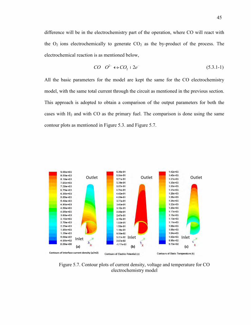
45

difference will be in the electrochemistry part of the operation, where CO will react with

the O2 ions electrochemically to generate CO2 as the by-product of the process. The

electrochemical reaction is as mentioned below,

22 2CO O CO e (5.3.1-1)

All the basic parameters for the model are kept the same for the CO electrochemistry

model, with the same total current through the circuit as mentioned in the previous section.

This approach is adopted to obtain a comparison of the output parameters for both the

cases with H2 and with CO as the primary fuel. The comparison is done using the same

contour plots as mentioned in Figure 5.3. and Figure 5.7.

Figure 5.7. Contour plots of current density, voltage and temperature for CO electrochemistry model

Contours of interface current density (a/m2)

Inlet

Outlet Outlet Outlet

Inlet Inlet

(a) (b) (c)

46

Figure 5.7-a. to c. compared to Figure 5.3. shows a small difference in the voltage

developed by the cell for both the cases. The cell voltage differs by just 0.1 V, with greater

value achieved using H2 as the fuel. It can still be considered that H2 contributes greater to

the electrochemistry when H2 and CO both are present in the fuel mixture, because of the

consumption of CO in the shift reaction, associated with the SOFC operation. The shift

reaction was not considered in the CO electrochemistry case and will be discussed in the

further section.

5.3.2. Modeling the Reformation and Water–gas Shift Reaction using CH4 as

Fuel. After checking the model for the CO electrochemistry case and the comparison of

the results for H2 and CO as the fuel, the same design was used to model the reformation

reactions and the water-gas shift reaction using hydrocarbon fuel methane (CH4). As

discussed in Section 1, solid oxide fuel cells possess this characteristic of using fuels other

than H2 for generating electricity. This model involves the integration of the chemical

reaction modeling with the other transport and conservation principles discussed earlier,

along with the UDF defined for the electrochemistry.

Humidified methane can be fed directly at the anode inlet of the SOFC model and

due to its high operating temperatures; methane reacts with the steam in the presence of

nickel which acts as the catalyst to generate CO and H2. This reaction is called as the

methane reformation reaction which is endothermic in nature. The reformation reaction is

shown in Equation (5.3.2-1),

47

4 2 23CH H O CO H (5.3.2-1)

The CO generated in the reformation reaction further reacts with the steam in the

mixture to produce more hydrogen and carbon dioxide as the by-product. In this case, both

the CO and H2 generated in the process take part in the electrochemical reactions and

contribute to the power produced. Equation (5.3.2-2) shows the Water-Gas shift reaction

mechanism.

2 2 2CO H O CO H (5.3.2-2)

The electrochemical reactions for hydrogen and CO are shown in Equations (1.1-1) in

Section 1 and (5.3.1-1), respectively.

Usually, for practical applications, methane is pre-reformed to a certain extent

before being fed at the inlet to the fuel cell. The high operating temperature of solid oxide

fuel cells provides the necessary heat energy for the initiation of the reformation reaction.

But the highly endothermic nature of this reaction generates large thermal gradients along

the path. This could result in high thermal stresses being induced in the materials used,

consequently affecting the life of the cell. To control and eliminate this problem, care is

taken to have a uniform distribution of the necessary species at the inlet to balance out the

thermal requirements of the processes involved. This is attained by having a partial

reformation process carried out prior to the fuel cell operation.

Stiller et al. [25] worked on a mathematical model for a tubular SOFC for the

partially pre-reformed methane case, for different operating conditions. The present model

48

was simulated using the same conditions for better comparison amongst different

operating parameters.

Table 5.1 shows the simulation parameters and results for the Stiller [25] model

and the present model for two different operating pressures.

Table 5.1. Comparison of results for the model with Stiller et al. [25]

Stiller

(atm)

Model

(atm)

Stiller

(press.)

Model

(press.)

Pressure (bar) 1.05 1.05 3.5 3.5

Inlet fuel temperature (K) 823 823 860 860

Inlet Air temperature (K) 1104 1104 1048 1048

Fuel utilization (%) 69 69 69 69

Inlet Fuel Composition :

H2 0.258 0.258 0.226 0.226

H2O 0.284 0.284 0.334 0.334

CH4 0.11 0.11 0.131 0.131

CO 0.057 0.057 0.057 0.057

CO2 0.228 0.228 0.241 0.241

N2 0.063 0.063 0.011 0.011

Voltage (V) 0.695 0.762 0.564 0.709

Average Current density (A/m2) 5000 7000

49

As mentioned earlier, the products obtained in the fuel stream after the partial pre-

reformation process is fed at the model inlet with the composition shown in Table 5.1. It

can be observed form the table that the current model performs better than the Stiller

model for similar set of operating and boundary conditions, considering the overall voltage

developed. This variation in the results can be due to various undeterminable parametric

differences in both the models. The total voltage is found to be lower for the pressurized

case, also needing a higher overall current through the circuit thus increasing the average

current density for the pressurized case. However, the results are found to be very sensitive

to the inlet temperature and the fuel composition.

Figure 5.8. Contour plots of the distribution of fuel species in the flow channel and on the electrolyte surface

Inlet

Outlet

Channel

Electrolyte

Interface

Inlet

Channel

Electrolyte

Interface

Outlet

(a) (b)

50

Figure 5.8. Contour plots of the distribution of fuel species in the flow channel and on the electrolyte surface (cont.)

Figure 5.8-(a-d). shows the contour plots of the distribution of the fuel species, as it

flows from the inlet to the outlet of the fuel cell. Figure 5.9. shows the variation of the H2O

mole fraction over the length of the cell. The distribution is analyzed in the anode flow

channel wall and the electrolyte surface on the anode side. Figure 5.8-a. shows the

distribution of CH4 over the length of the cell; it can be seen that the concentration

gradually goes on decreasing with a good overall distribution along the length for the

given set of conditions. The reformation reaction taking place (Equation 5.3.2-1) uses up a

portion of the steam contained in the mixture and produces CO and H2 which can be seen

in Figure 5.8-b and 5.8-d. There is an increase in the CO fraction at the start of the

Inlet

Channel

Electrolyte

Interface

Outlet

Inlet

Channel

Electrolyte

Interface

Outlet

(c) (d)

51

electrolyte interface, which is further consumed in the electrochemistry and also for the

shift reaction. It is noted that the shift reaction is more dominant further down the line i.e.

closer to the outlet, producing more CO2 and H2 closer to the outlet as seen in Figure 5.8-c

and 5.8-d.

Figure 5.9. Plot showing distribution of H2O along length of the cell

Figure 5.9. shows the distribution of H2O along the fuel cell length. The decrease

in the concentration is due to the consumption of H2O in both the reformation and the shift

reactions, but the electrochemical reaction involving H2 prevents the H2O concentration

from falling considerably over the cell length.

0.00

0.05

0.10

0.15

0.20

0.25

0.30

0.000.020.040.060.080.100.120.14

H2O mole fraction


H2O

Mo

le f

ract

ion

(m

ol/

mo

l)

52

The chemical reactions are modeled using the finite rate model in the FLUENT

solver. The activation energies for the reactions are specified approximately, based on the

values mentioned in the literature. The activation energy for the reformation reaction is

considered in the range of 60-230 kJ/mol [31] and for the shift reaction it’s considered to

be 100-300 kJ/mol [31-32]. Figure 5.10-(a-b). shows the contour plots for the kinetic rates

of reaction for the reformation reaction (reaction 1) and the shift reaction (reaction 2)

respectively.

Figure 5.10. Contour plots for kinetic rates of reaction

Figure 5.10. indicates that both the reactions were dominant in the flow channel

where there was enough concentration of the reactants and the high temperature to carry

out the reactions. Figure 5.10-b. shows that the shift reaction becomes dominant along the

Methane reformation reaction Shift Reaction

(a) (b)

53

length of the cell when there is more CO and H2O produced from the reformation reaction

and the electrochemical reaction down the line. As mentioned earlier, the strongly

endothermic nature of the reformation reaction makes the temperature fall considerably in

the channel and then increases again due to the exothermic electrochemical reaction and

the shift reaction.

Thus, the computational model used in this study, helps understand and analyze the

processes involved in the SOFC operation much more descriptively as compared to other

modeling approaches. Lowering the initial temperatures in this case can prove to be

helpful to reduce the high thermal gradients generated due to the reactions and also

catalysts can be used to control the activation requirements i.e. ultimately the kinetics

involved in the reactions.

54

6. CONCLUSIONS AND FUTURE WORK

This thesis work included a detailed computational fluid dynamics modeling,

simulation and analysis of a tubular solid oxide fuel cell. A cathode supported structure

was developed using a FLUENT pre-processor software GAMBIT 2.3.16. The meshed

structure was then modeled for fluid flow, mass transport and electro-thermo-chemical

analysis using the FLUENT 12.0 interface including the SOFC UDF developed by

FLUENT for modeling the electrochemical reactions occurring in the SOFC’s. Some

important discussions based on the analyses of the model for the different conditions are

mentioned in the following sections.

6.1. CONCLUSIONS AND DISCUSSIONS

The results obtained from the analyses performed on the model for the different

conditions mentioned in the previous sections show that the computational model

developed is much more advantageous for understanding the complex processes involved

in the SOFC operation. The plots and results obtained are much more descriptive in terms

of the distribution of various important parameters in a three dimensional perspective.

A parametric analysis was performed on the model, to analyze its response and

performance to varying parameters. By the temperature effect study, it was discovered that

the model showed a greater overall operating potential at a lower temperature compared to

the other cases for the specific set of basic properties defined. This characteristic of the

model makes it suitable to be used as a prototype for an intermediate temperature SOFC

55

for further analysis. An optimum operating temperature combined with suitable electrolyte

thickness was observed for the given model [33].

For further exploring the advantages of solid oxide fuel cells, the model was

simulated for cases using fuels other than hydrogen, to analyze the performance. The

simulation was carried out successfully, describing the reformation reaction and the shift

reaction for methane as the fuel. The simulation results were studied for a single case,

evaluating the effect of the specified parameters. Since, no complete set of input

parameters and experimental results are found in the literature for tubular fuel cells, the

obtained correspondence can be considered sufficient for the validation. Based on all the

analyses, the model could be used as a base model or a prototype of a cathode supported

tubular SOFC, to carry out a faster and cheaper analysis prior to a successful experimental

setup.

6.2. FUTURE WORK SUGGESTIONS

The SOFC model mentioned in this work was evaluated considering a few

assumptions mentioned in Section 3. The steady state models used in these analyses can be

replaced by adopting a transient analyses approach. FLUENT itself provides the option of

setting-up a transient case using its implicit solver. A complete transient analysis can be

very helpful in analyzing the kinetics of each reaction and also the flow duration for

different composition and flow rates of the fuel and oxidizer. Also, as discussed in Section

2, a radiation model can be included to account for the effect of radiation heat transfer on

the final operating temperature of the cell, which was neglected in the present model. The

integration of the chemical reactions with the electrochemical model can be studied in

56

detail, by considering different rate limiting reactions, and also by modifying the catalytic

effect on the reactions involved.

This single cell model can be further modified to be used as an appropriate pre-

evaluation tool by upgrading it to a complete fuel cell stack, with all necessary parts

involved in the operation. A complete stack model, will evaluate the performance most

accurately compared to any other single cell models.

These important additions to the model can help considerably in this research area

of solid oxide fuel cell modeling. These computational setups can be simulated for

different parameters and conditions and the results can be analyzed and used for

optimizing the performance of the fuel cell systems.

57

APPENDIX

FLUENT TUTORIAL FOR SETTING UP THE TUBULAR SOFC MODEL

The Solid Oxide Fuel Cell Unresolved electrolyte module was developed by

FLUENT for modeling and simulating 3-D SOFC designs. A license for this module is

needed to be bought separately for the unresolved electrolyte. The steps mentioned below

will help in complete setup and modeling of a SOFC design using FLUENT.

Step 1: Importing the mesh and starting up the SOFC module

Start FLUENT 12.0 using the 3-D double precision model.

Read the mesh file for the model from the location.

(FILE READMESH)

Scale the mesh according to the case requirement

(Problem setupGeneralMeshScale)

The Solid Oxide Fuel Cell (SOFC) With Unresolved Electrolyte Model is

loaded into ANSYS FLUENT through the text user interface (TUI). The

module can only be loaded after a valid ANSYS FLUENT mesh or case file

has been set or read. The text command to load the addon module is

define models addon-modules

A list of FLUENT addon modules is displayed as shown below:

FLUENT Addon Modules:

0. None

1. MHD Model

2. Fiber Model

58

3. Fuel Cell and Electrolysis Model

4. SOFC Model with Unresolved Electrolyte

5. Population Balance Model

Enter Module Number: [0] 4

Select the SOFC Model with Unresolved Electrolyte by entering number 4, which

will load the SOFC module for the selected model.

Step 2: Case setup for the fluid flow, species transport and the heat transfer

For simplicity in recognizing the zones in the tubular model, rename the

electrolyte zone to electrolyte-cathode and the electrolyte shadow zone to

electrolyte-anode.

Check the display and the grid ( correct the mesh if any discrepancies observed

in the quality of the mesh)

Retain the solver settings with a pressure-based and steady state solver.

Turn on the heat transfer analysis tool by enabling the energy equation

Problem setup Models Energy

Enable laminar flow simulation, ensuring that the viscous heating is disabled.

Problem setup Models Viscous

59

Define the species transport and reaction models.

60

Enable the species transport model for volumetric reactions and also enable the

Diffusion Energy Source, Full Multicomponent Diffusion and the Thermal

Diffusion models.

Step 3: Setting up the electrochemical model using the FLUENT UDF (the values

mentioned in the brackets are an example for the present tubular model)

Problem SetupModelsSOFC (Unresolved Electrolyte) Edit

61

Specify the Current Underrelaxation Factor for the solver for the given case

Set the Total System Current or the Specified System Voltage, as per the output

requirement

Set the Leakage Current Density, Electrolyte Resistivity and the Electrolyte

Thickness as per the case requirement.

Enable the Electrolyte Conductivity Submodel, Volumetric Energy Source,

Surface Energy Source, Species Sources and disable the CO Electrochemistry

(for H2 as the fuel) models in the Model Options section.

In the Electrochemistry tab, define the Exchange Current Densities,

Concentration Exponents (obtained from the electrochemical reaction) and the

Butler Volmer Coefficients

62

Define the zones having the anode and the cathode interface and also the

tortuosity values can be set for specific zones in the Electrolyte and Tortuosity

tab.

63

In the Electric Field tab,

Define upto 5 conductive zones with their conductivities

Define upto 3 contact surfaces with the surface resistance values

Specify the voltage and the current tap surfaces

Step 4: Specify the Material Properties

Define a User-defined scalar, by changing the number of user-defined scalars to

1

DefineUser-definedScalars

Define 14 user-defined memory locations for storing the user-defined parameter

values

DefineUser-definedMemory

Define user-defined function hooks by changing the Adjust function to

adjust_function

DefineUser-definedFunction hooks

Create or re-define new solid materials as appropriate for the electrodes and the

electrolyte according to the problem specifications.

64

Edit the mixture template by specifying the mixture species as per the case

setup

1. Using H2 as the fuel:

In the Species dialog, arrange the materials under Selected Species in

the following order: h2o, o2, h2, and n2.

MaterialsCreate/Edit materialsMixture Species

(Copy the properties for H2 from the fluent database)

2. Using partially pre-reformed CH4 as fuel:

65

Arrange the species in the increasing order of their specified compositions

in the mixture species box.

CH4, when used as the fuel also involves chemical reactions along with the

electrochemical part. The reactions are modeled using the FLUENT solver,

which needs the user the feed in the values of the parameters needed for the

reaction such as the activation energies and the pre-exponential factor,

which are needed for the calculation of the reaction rates.

MaterialsCreate/EditMixture templateReaction

Change the Thermal conductivity and Viscosity to ideal-gas mixing law.

Change the Mass Diffusivity to user-defined and select diffusivity::SOFC as

the user-defined function.

66

Change the UDS Diffusivity to user-defined and select E_Conductivity::SOFC

as the user defined function.

Step 5: Setting up the Operating and Boundary Conditions

Problem SetupCell-zone conditionsOperating Conditions

Boundary Condition specifications

1. Using H2 as the fuel:

The anode and the cathode properties are set as shown in the screenshot above.

The source terms are decided as per the case setup and the electrochemical

reactions. The electrodes are modeled as porous zones by specifying the

percent porosity of the zones.

Change the material for the current collectors to current-collector-material.

67

Problem SetupBoundary Conditionsinlet

The inlet properties for the anode are specified, flow rate is calculated as per

the case setup. Species composition and distribution is specified in the Species

tab. Similarly the cathode inlet properties are specified.

The operating temperature can be specified in the Thermal tab.\

3. Using partially pre-reformed CH4 as fuel:

68

The source terms in this case are specified for the anode and the cathode zones

in a similar manner.

The inlet conditions for the anode and the cathode in this case is specified in a

manner similar to the H2 case. The mole fractions of the species at the inlet are

fed in the Species tab.

Step 6: Solution Methods and controls

Problem SetupSolution Methods

Select the SIMPLE pressure-velocity coupling scheme with a Green-Gauss Cell

Based discretization method.

Select Standard for pressure and First Order Upwind scheme for momemtum,

Energy and all the species for the case.

Use the default under-relaxation factors for all parameters, unless required to be

changed to rectify errors

Problem SetupMonitors

Turn on the residual monitors and set the convergence criteria as shown or as

per requirement

69

Step 7: Initialization and simulating the model

Initialize the flow field for all the zones.

Problem SetupSolution InitializationInitialize

Run the simulation until the residuals converge.

Problem SetupRun Calculation

Step 8: Postprocessing

Carry out the postprocessing of the electrochemical parameters as per the chart

mentioned below [29]:

UDM-0 Interface Current Density (A/m2)

UDM-1 Nernst Potential (Volts)

UDM-2 Activation Overpotential (Volts)

UDM-3 Volumetric Ohmic Source (W/m3 )

UDM-4 x Component of the Current Density (A/m2)

UDM-5 y Component of the Current Density (A/m2)

UDM-6 z Component of the Current Density (A/m2 )

UDM-7 Electrolyte Voltage Jump

UDM-8 Electrolyte Resistivity (Ohm-m)

UDM-9 Effective Electric Resistance

UDM-10 Anode Activation

UDM-11 Cathode Activation

UDM-12 Electrochemical Source (W/m3 )

UDM-13 Magnitude of Current Density (A/m2 )

70

BIBLIOGRAPHY

1. History of Fuel cells. Available from: www.sae.org/fuelcells/fuelcells-history.htm.

2. R O'Hayre, Suk-Won Cha, W Colella, F Prinz, Fuel Cell Fundamentals. 2009, New York: John Wiley & sons

3. S Singhal, K Kendall, High Temperature Solid Oxide fuel cells: Fundamentals, design and applications. 2003: Elsevier Ltd.

4. S Supramaniam, Fuel Cells: From fundamentals to applications. 2006: Springer.

5. Fuel Cell Handbook, U.S.D.o. Energy, Editor. 2004, EG&G Technical Services.

6. H Karoliussen, K Nisancioglu Mathematical modeling of cross plane SOFC with internal reforming. in Proceedings of the third international symposium on SOFC. 1993. Honolulu, Hawaii.

7. E Achenbach, Three-dimensional and time-dependent simulation of a planar solid oxide fuel cell stack. Journal of Power Sources, 1994.

8. S Kakac, A Pramuanjaroenkij, Xiang Yang Zhou, A review of numerical modeling of Solid Oxide fuel cells. International Journal of Hydrogen Energy, 2006.

9. N Bessette II, W Wepfer, J Winnick, A Mathematical model of a Solid Oxide Fuel Cell. Journal of Electrochemical Society, 1995. 142(11).

10. P Costamagna, E Arato, E Achenbach , U Reus, Fluid Dynamic study of fuel cell devices: simulation and experimental validation. Journal of Power Sources, 1994. 52.

11. SH Chan, K Khor, ZT Xia, A complete polarization model of a solid oxide fuel cell and its sensitivity to change of cell component thickness. Journal of Power Sources, 2001. 93.

12. C Ding, H Lin, K Sato, K Amezawa, T Kawada, J Mizusaki, T Hashida, Effect of thickness of Gd0.1Ce0.9O1.95 electrolyte films on electrical performance of anode-supported solid oxide fuel cells. Journal of Power Sources, 2010. 195.

13. Chan-Yeup Chung, Yong-Chae Chung, Performance characteristics of a micro single-chamber solid oxide fuel cell: Computational Analysis. Journal of Power Sources, 2005. 154.

14. N Akhtar, S Decent, D Loghin, K Kendall, A three-dimensional numerical model of a single-chamber solid oxide fuel cell. International Journal of Hydrogen Energy, 2009. 34.

71

15. H Yakabe, T Ogiwara, M Hishinuma, I Yasuda, 3-D model calculation for planar SOFC. Journal of Power Sources, 2001. 102.

16. K Recknagle, R Williford, L Chick, D Rector, M Khaleel, Three-dimensional thermo-fluid electrochemical modeling of planar SOFC stacks. Journal of Power Sources, 2003. 113.

17. S Murthy, A Fedorov, Radiation heat transfer analysis of the monolith type solid oxide fuel cell. Journal of Power Sources, 2003. 124.

18. Y Lin, S Beale, Performance predictions in Solid Oxide Fuel Cells, in Third International Conference on CFD in the Minerals and Process Industry, CSIRO. 2003: Melbourne, Australia.

19. Zuopeng Qu, P Aravindh, N Dekker, A Janssen, N Woudstra, A Verkooijen, Three-dimensional thermo-fluid and electrochemical modeling of anode-supported planar solid oxide fuel cell. Journal of Power Sources, 2010. 195.

20. W J R Fang, R Dougal, J Khan, Thermoelectric model of a Tubular SOFC for Dynamic simulation. Journal of Energy Resources Technology, 2008. 130.

21. S Campanari, P Iora, Definition and sensitivity analysis of a finite volume SOFC model for a tubular cell geometry. Journal of Power Sources, 2004. 132.

22. R Suwanwarangkul, E Croiset, M Pritzker, M Fowler, P Douglas, E Entchev, Mechanistic modeling of a cathode supported tubular solid oxide fuel cell. 2005.

23. R Suwanwarangkul, E Croiset, M Pritzker, M Fowler, P Douglas, E Entchev, Modeling of a cathode-supported tubular solid oxide fuel cell operating with biomass-derived synthesis gas. Journal of Power Sources, 2007.

24. Y M Barzi, M Ghassemi, M Hamedi, A 2D transient numerical model combining heat/mass transport effects in a tubular solid oxide fuel cell. Journal of Power Sources, 2009. 192.

25. C Stiller, B Thorud, S Seljebo, O Mathisen, H Karoliussen, O Bolland, Finite-volume modeling and hybrid-cycle performance of planar and tubular solid oxide fuel cells. Journal of Power Sources, 2004. 141.

26. N Autissier, D Larrain, J Van Herle, D Favrat, CFD simulation tools for solid oxide fuel cells. Journal of Power Sources, 2003. 131.

27. U Pasaogullari, Chao-Yang Wang, Computational Fluid Dynamics modeling of solid oxide fuel cells. Electrochemical society, 2003.

28. A Sleiti, Performance of tubular Solid Oxide Fuel cell at reduced temperature and cathode porosity. Journal of Power Sources, 2010. 195.

29. Fuel cells Module Manual 12.0, ANSYS, Editor. 2009.

72

30. A Hagiwara, H Michibata, A Kimura, M Jaszcar, G Tomlins, Veyo SE. Tubular Solid Oxide Fuel cells life test. in Proceedings of third international fuel cells conference. 1999. Nagoya, Japan.

31. K Ahmed, K Foger, Kinetics of internal steam reforming of methane on Ni/YSZ-based anodes for solid oxide fuel cells. Catalysis Today, 2000. 63(479-487).

32. F Bustamante, R Enick, R Killmeyer, B Howard, K Rothenberger, A Cugini, B Morreale, M Ciocco, Uncatalyzed and wall catalyzed forward water-gas shift reaction kinetics.

33. S Puthran, U Koylu, S Hosder, F Dogan, Three-dimensional CFD modeling of tubular solid oxide fuel cell using different fuels, in 5th International Energy Sustainability and Fuel Cell conference, ASME, 2011. 2011: Washington DC.

73

VITA

Sachin Laxman Puthran received his B. Tech in Mechanical Engineering from

Vidyavardhini’s College of Engineering and Technology affiliated to the Mumbai

University, India in May 2007. Soon after that, in July 2007, he joined Jindal Drilling and

Industries Ltd. as a MWD (Measurement While Drilling) Engineer. Duties included

working on-field at oil drilling rigs, operating an electro-magnetic depth and direction

measurement tool in directional drilling services. Later worked as an instructor at JTG

Classes, teaching mathematics to secondary and higher secondary level students from

November 2008 to July 2009. In August 2009, he joined the Mechanical and Aerospace

Engineering Department at Missouri University of Science and Technology for the

Master’s in Mechanical Engineering program. He completed his M.S in Mechanical

Engineering in August 2011.

He has presented a conference paper at the 5th International Energy Sustainability

and Fuel Cell Conference by ASME, 2011, Washington DC. His graduate research

included Computational Fluid Dynamics (CFD), simulation softwares, modeling and

analysis of Solid Oxide fuel cells. Other interests include fuel cell applications,

renewable energy research and fluid dynamic applications. Sachin has been a student

member of ASME.

Documents

3-DIMENSIONAL COMPUTATIONAL FLUID CELL USING DIFFERENT FUELS by SACHIN LAXMAN … · 3-dimensional computational fluid ... cell using different fuels . by . sachin laxman puthran