Embed Size (px)
Citation preview
Remote Sens. 2011, 3, 721-751; doi:10.3390/rs3040721
Remote Sensing ISSN 2072-4292
www.mdpi.com/journal/remotesensing
Article
3-Dimensional Building Details from Aerial Photography for
Internet Maps
Philipp Meixner * and Franz Leberl
Institute for Computer Graphics and Vision, Graz University of Technology, Inffeldgasse 16,
8010 Graz, Austria; E-Mail: [email protected]
* Author to whom correspondence should be addressed; E-Mail: [email protected];
Tel.: +43-316-873-5035; Fax: +43-316-873-5050.
Received: 5 January 2011; in revised form: 1 February 2011 / Accepted: 11 February 2011 /
Published: 8 April 2011
Abstract: This paper introduces the automated characterization of real estate (real
property) for Internet mapping. It proposes a processing framework to achieve this task
from vertical aerial photography and associated property information. A demonstration of
the feasibility of an automated solution builds on test data from the Austrian City of Graz.
Information is extracted from vertical aerial photography and various data products derived
from that photography in the form of a true orthophoto, a dense digital surface model and
digital terrain model, and a classification of land cover. Maps of cadastral property
boundaries aid in defining real properties. Our goal is to develop a table for each property
with descriptive numbers about the buildings, their dimensions, number of floors, number
of windows, roof shapes, impervious surfaces, garages, sheds, vegetation, presence of a
basement floor, and other descriptors of interest for each and every property of a city. From
aerial sources, at a pixel size of 10 cm, we show that we have obtained positional
accuracies in the range of a single pixel, an accuracy of areas in the 10% range, floor
counts at an accuracy of 93% and window counts at 86% accuracy. We also introduce 3D
point clouds of facades and their creation from vertical aerial photography, and how these
point clouds can support the definition of complex facades.
Keywords: aerial images; 3D-modeling of buildings; semantic image interpretation;
counting building floors; window detection; real estate valuation; facade point clouds
OPEN ACCESS
Remote Sens. 2011, 3
722
1. Describing Real Properties
We define a ―real property‖ by one or sometimes multiple parcels as they are recorded in cadastral
maps. It consists of a piece of land, sometimes defined by a fence, on which are one or more buildings,
impervious surfaces, garages, trees and other vegetation. A property may also contain only the portion
of a multi-unit building, for example in dense urban cores where buildings are connected.
The description of a real property consists of a table with coordinates and numbers. These define the
number of buildings, type of building from a stored list of candidates, building height and footprint,
number of floors, number and types of windows, presence of a basement floor, type of attic, roof type
and roof details such as an eave, skylights, chimneys, presence of a garage and its size, types and
extent of impervious surfaces, such as a driveway and parking spaces, and statements about the type
and size of elements of vegetation, the presence of a water body, the existence and type of a fence,
exposure to the sun and effects of shadows, the quality of views from a window, etc.
We expect that such information per parcel, for all properties of a city, will be useful for a broad
range of applications in city administrations, commercial location-based services and searches on the
Internet [1]. There will, however, be concern about the cost of data creation. An economically
favorable approach would build first of all on the wealth of already existing routine aerial photography
justified by other applications, not insignificantly in connection with innovative location-aware global
Internet sites such as Google Maps and Microsoft’s Bing Maps, or the innumerable regional sites.
Secondly, such property-descriptions will need to be developed automatically, with little
manual support.
Therefore we have designed a processing framework which focuses on using pre-existing high
resolution vertical aerial images and cadastral data. These two sources need to be conflated into a
common coordinate system. The aerial images themselves in turn are the source of terrain models,
image camera poses and classifications. One may possibly also involve street vectors. The process first
builds an integrated geometry and semantic object data set which can then be analyzed for the
development of descriptors. Our initial results concern the definition of building details. We show that,
for vertical aerial photography, we have achieved an accuracy in counting floors of 93%, and for
windows 86%.
2. Inspiration from the Location-Aware Internet
2.1. Evolving from Digital Geodata to Location-Awareness
A location-aware Internet [2-5] has evolved since about 2005. Internet-search has been a driving
force in the rapid development of detailed 2-dimensional maps and also 3-dimensional urban models.
―Internet maps‖ in this context consist of street-maps used for car navigation, augmented by the terrain
shape in the form of the Bald Earth and all this accompanied by photographic texture from ortho
photos. This is currently available for large areas of the industrialized World when calling up the
websites maps.google.com or www.bing.com/maps, and also from a number of regional Internet
mapping services, for example the French www.geoportail.fr or the German
www.klicktel.de/kartensuche.
Remote Sens. 2011, 3
723
The transition from the first availability of digital map data to today’s interactive location-based
search on the Internet spans about 30 years. One may divide the evolution into several distinct stages:
(1) The massive transition to digital geo data dates back to the time when computing facilities were
first able to cope with the data quantity implied in the geo-application and began with the
scanning of paper maps and their subsequent vectorization in the late 1970s. This improved the
storage, retrieval, transmission and printing of such data.
(2) The availability of digital data led to an early form of pre-Internet e-commerce by shipping
shrink-wrapped Geodata to interested experts.
(3) Road maps became available for trip planning in the mid 1990s, initially for transportation
systems, later for the general public in the form of car navigation. It required the broad
acceptance of personal computing. Geodata were transported on digital media.
(4) The Internet was the major enabler of the widespread commerce with Geodata greatly
improving the convenience in exchanging orthophotos, aerial and satellite photography.
Shrink-wraps were replaced by online services.
(5) The GPS (Global Positioning System) inspired a further increase in the usefulness of digital
Geodata and resulted in the transition to true real-time navigation from about the mid 1990s
onwards, based on street maps.
(6) The latest stage of this evolution was the introduction of Geodata into the novel
search-application via the Internet. Global location awareness was introduced into Internet
search via maps.google.com and www.bing.com/maps. 3D urban building models came into
being in November 2006 with Microsoft’s announcement of the availability of Virtual Earth
in 3D [6].
(7) We see today the emergence of smart telephones and a refined interest in locations, not only in
cars but now also for pedestrian applications.
An interesting transition occurred along the way from Geodata as a realm of experts, into routine
use by everyone. This separate evolutionary track began with a very early idea, namely the invention
of the GIS (Geographic Information Systems) in about 1962 [7]. The idea was born well ahead of the
ability to realize it in the form of large area systems. While of course entirely predicated on the
availability of the computer, it took the personal computer to make the idea a practical reality.
However, the GIS did not change the basic limitations of ―Geodata for the experts‖. That change
became very visible with the development of car navigation systems for regular passenger cars. It
signaled for the first time a transition from experts to everyone. This development accelerated with the
location-aware Internet search, so that today almost every Internet user is also a user of Geodata,
inspecting and judging aerial photography, oblique imagery, 3D building models and, most recently,
also street-side images and their various methods of supporting a Geo-naïve user.
Urban 3D models have been a research topic since the mid 1990s [8-12]. The initial introduction
into Internet-search at Bing Maps (then Virtual Earth) employed man-made buildings as triangulated
point clouds with a visual embellishment by photographic texture. Since April 2008, vegetation is
being classified and identified, and computer-generated vegetation is being placed on top of the Bald
Earth [5].
Remote Sens. 2011, 3
724
3D urban models are still in their infancy and are provided over large areas only by Bing Maps, with
an example presented in Figure 1 in its ―classic‖ version from www.bing.com/maps. Recently, the
emphasis has shifted at Microsoft from a full 3D urban model to the use of 2D street-side imagery that
has undergone some limited 3D processing (see www.bing.com/maps/explore). While Internet-search
may be the most visible and also initial driving application, there are of course others. Often mentioned
are city planning, virtual tourism, disaster preparedness, military or police training and decision
making [13], or 3D car navigation [14]. In Germany, 3D building models are being considered of such
municipal relevance that a fairly complex and all-encompassing CityGML data standard has been
developed to guide the creation of 3D building models at various levels of detail, ranging from a basic
L0 through to a virtual reality level L4 with indoor 3D modeling [15]. This standard has been adopted
by the international Open Geospatial Consortium (OGC) [16].
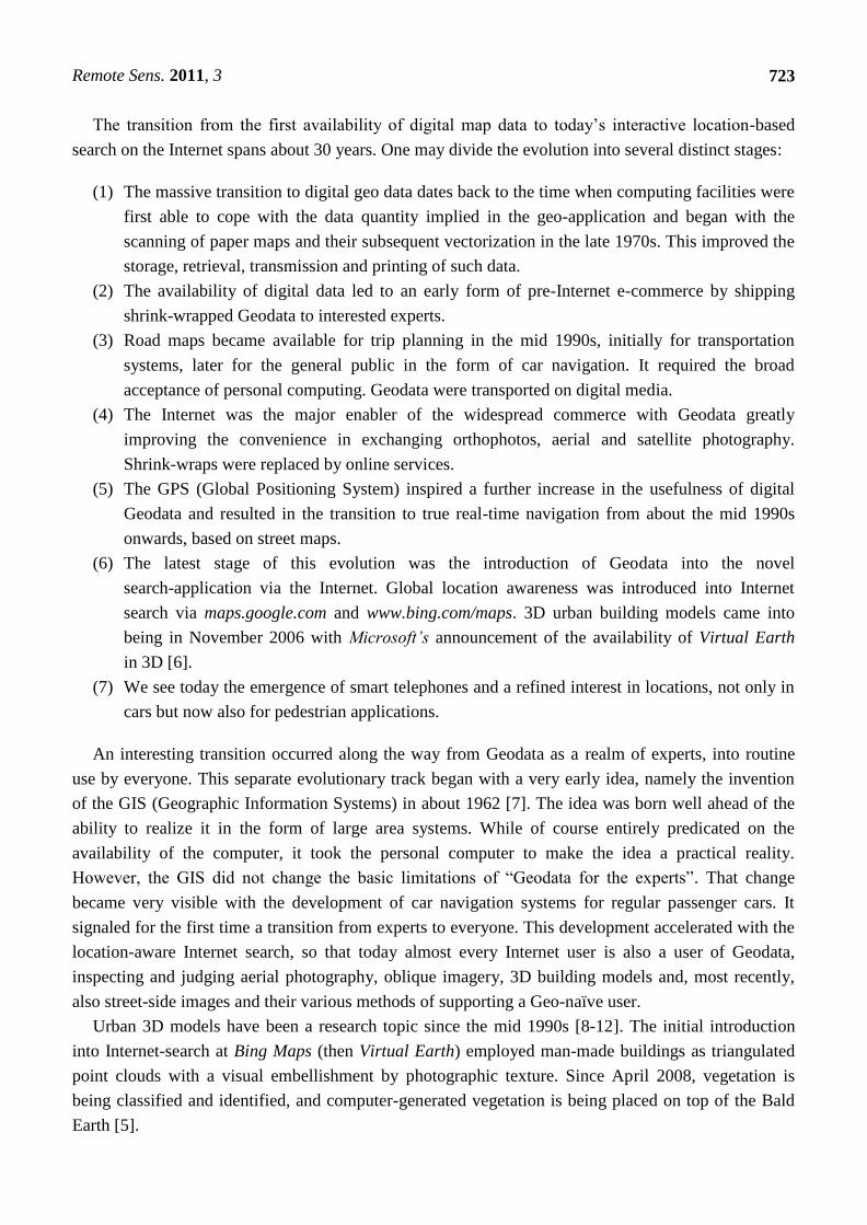
Figure 1. Typical 3D content in support of an Internet search, taken from
www.bing.com/maps. The focus is on providing a pleasant ―user experience‖. The example
is the Colorado State Capitol. The geometry is from vertical aerial photography, the
photo-texture from separate aerial oblique imagery. The vegetation has been classified and
computer generated trees have been placed at the locations classified as trees.
2.2. Towards Semantically Interpreted Urban Models
So-called 3D-location awareness of the Internet serves to please the user’s eye—one could speak of
―eye candy‖—but cannot be used as part of the search itself. This is unlike the 2D content with its
street map and address codes that can be searched. An interpreted urban 3D model would support
searches in geometry data, not just in alphanumeric data. Certain characteristics may be interest, such
as: the number of buildings higher than four floors in a certain district, a built-up floor area in excess
of 500 m2, impervious areas at less than 30% of the land area, large window surfaces in excess of 30%
of the wall surface, a certain minimum sun exposure during the day, with attractive views of the distant
urban landscape.
We can search for such objects if we augment the Internet with descriptions of real properties.
Image contents must not merely be shown on a monitor, but they must get interpreted. For this to be
Remote Sens. 2011, 3
725
accomplished at low cost, it must be done automatically and from easily available sources. We are
facing a research challenge for computer vision [4,17].
2.3. Growing from Location-Awareness towards Ambient Intelligence
While applications like Bing Maps or Google Earth are currently driven to engage the public in
using the associated Internet-search systems via attractive location awareness, there is a deeper
justification in light of the emerging opportunities created by the Internet-of-Things and Ambient
Intelligence. Both concepts need location awareness [18]. Already in 1991, Marc Weiser authored his
much quoted prediction for computing in the 21st century and postulated that location will be one of
two issues of crucial importance: ―ubiquitous computers must know where they are‖ [19].
Weiser’s sketch of the future has morphed from ubiquitous computing to ambient intelligence. We
expect the geometry of the elementary parts of an entire urban environment to be available at a human
scale to be searched; we foresee that this becomes the basis for locations of fixed sensors, or moving
GPS-tracked sensors, to read the RFID- and other tags of goods to be placed inside buildings, even
inside individual rooms. In analogy, triangulated cell phones as well as tags can also place persons
inside buildings and rooms. A semantically interpreted 3D city model could help find one’s briefcase,
an errant person, the nearest copying machine and will affect the use and behavior of all sorts of
computer-driven gadgets.
3. Going through a Processing Framework
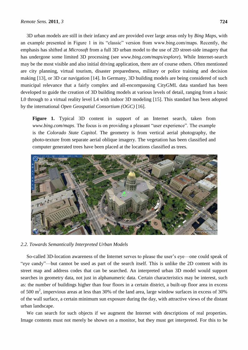
Low cost by automation and a reliance on pre-existing sources has led us to define a general
processing framework (Figure 2). We start out by conflating (merging) geometric data from essentially
two sources: the aerial imagery and the cadastral information. Figures 3 and 4 cover an example of a
400 m × 400 m urban test area in the city of Graz (Austria). Conflation defines each property as a
separate entity for further analysis, not unlike previous authors have proposed [20]. The cadastral data
may also contain preliminary information about a 2D building footprint. Conflation is part of a
pre-processing workflow and results in all geometric data being available per property and in a single
geometric reference system.
We now proceed towards the use of the dense 3D point clouds associated with the aerial
photography and extracted from it by means of a dense matcher applied to the triangulated aerial
photographs [21]. ―Dense‖ refers to the fact that each image pixel gets assigned a terrain elevation
value. The surface model is thus at a spacing equal to the Ground Sampling Distance (GSD) of the
images. The extraction of data per building and per element of vegetation comes first. This finds the
areas occupied by a building as well as its height. For vegetation we need to find the type, its location,
the height and the crown diameter. The building footprints get refined vis-à-vis the cadastral prediction
using image segmentation and classification to define roof lines.
From the building, one proceeds to the facades: building footprints become facade baselines. A
decision is needed on the number of facades. We segment a single building shape so that the footprints
of its parts all consist of simple rectangular shapes. This is the basis for addressing the facades. For
each facade we must find its intersection with the ground—its footprint. This is the basis for an
extraction of the facade in 3D by intersecting it with elevation data. We compute the corner points of
Remote Sens. 2011, 3
726
each facade. These can then be projected into the block of overlapping aerial photography. We can
search all aerial images for the best representation of the facade details; typically this will be the image
with the maximum number of pixels for a given facade. Since there are multiple facade images, we
prepare for a multi-view process.
Figure 2. Diagram of the proposed work flow to characterize real properties from aerial
images and associated cadastral data (performed processing steps highlighted).
What follows is a search for rows and columns of windows in the overlapping (i.e., ―redundant‖)
photographic imagery. First of all, this serves to establish the number of floors. Second, we also are
interested in the windows location themselves, as well as in their size. And finally, we want to take a
look at attics and basement windows to establish whether there is an attic or basement.
While Figure 2 summarizes the workflow, subsequent sections of this paper will fill in the details
based on sample data from Figures 3 and 4 from the City of Graz to explain the approach. The aerial
coverage is taken with a ground sampling distance at 10 cm and with overlaps of 80% forward and
Aerial Images DTM/DSM
Orthophoto AT
Segmented Images (WGS84 Coordinate System)
Cadastre (Gauss Krueger) Street Networks (Display
Coordinate System
Assembling Data per property Chamfer Matching and Coordinate Transformations
Classified Image Segments per property and per building
DTM/DSM, Orthophoto, Segmented Images
Determination of roof details Roof type, Eaves, Skylights,
Chimneys, Type of attic
Roof Details Type, Eaves, Skylights, Chimneys, Sun Hours
Detection of other facade details Garages, bays, stucco, balconies
Location of garages, bays and type of stucco
Window detection, floor determination
Number and location of windows
Floor number
Location, Size and Type of Trees and
Hedges Roofs per building
Location and size of impervious surfaces, swimming pools, etc.
Semantic description per property Facade determination (2D and 3D) Decomposing of complex buildings
into separate objects Determination of Building heights
Tree and Vegetation Detection Heights and crown diameter
Type of Tree (conifer, broadleaf)
Determination of impervious surfaces, water bodies, etc
Facades per building
Remote Sens. 2011, 3
727
60% sideward. Our aim is to show that an automated property characterization is feasible, not least due
to the fact that the overlaps produce a10-image coverage of each terrain point.
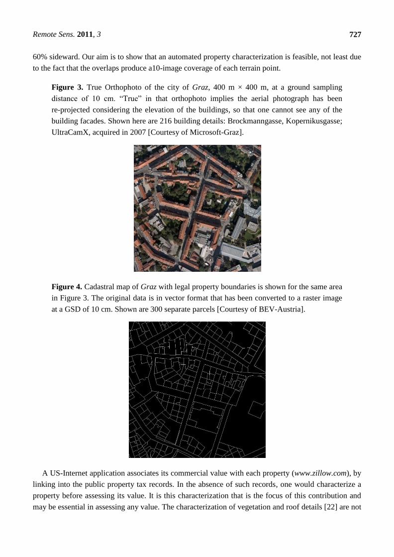
Figure 3. True Orthophoto of the city of Graz, 400 m × 400 m, at a ground sampling
distance of 10 cm. ―True‖ in that orthophoto implies the aerial photograph has been
re-projected considering the elevation of the buildings, so that one cannot see any of the
building facades. Shown here are 216 building details: Brockmanngasse, Kopernikusgasse;
UltraCamX, acquired in 2007 [Courtesy of Microsoft-Graz].
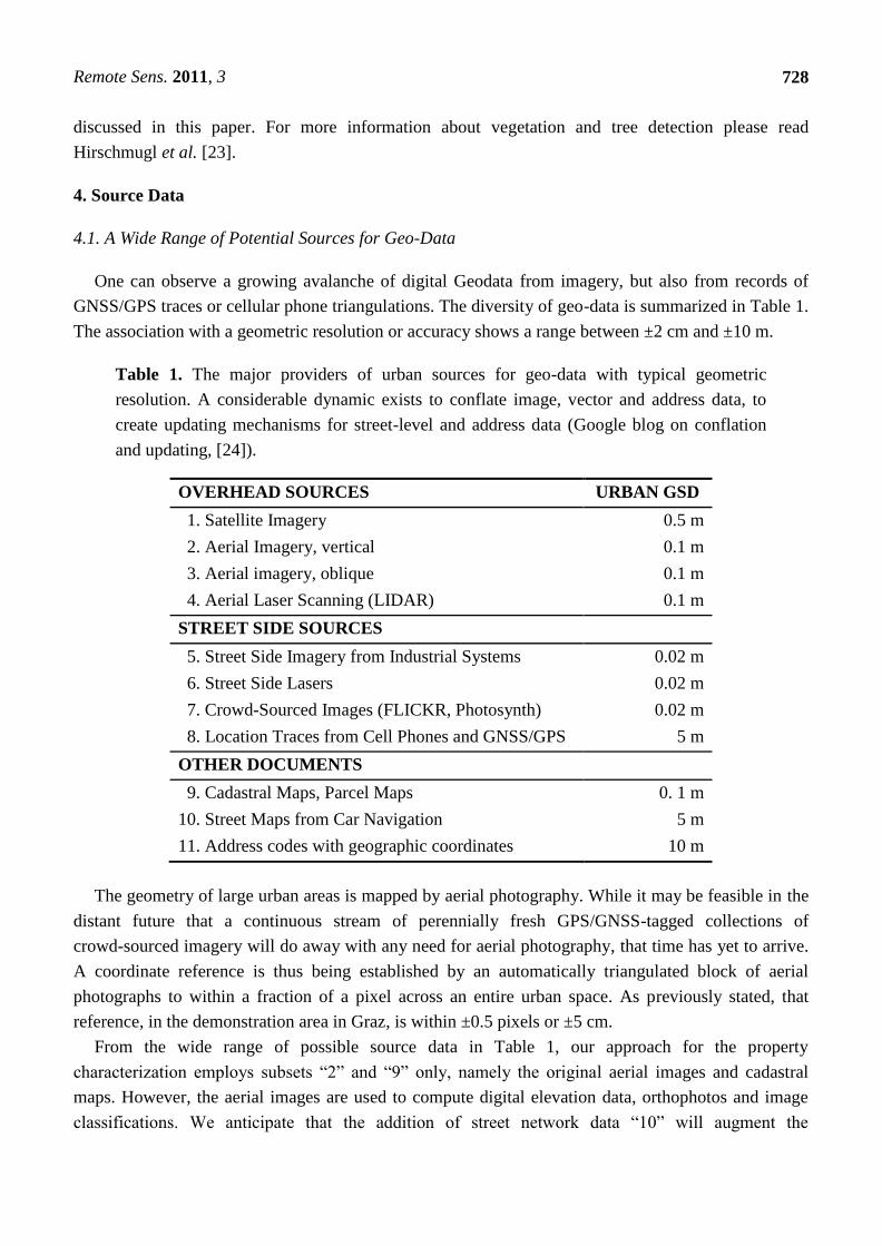
Figure 4. Cadastral map of Graz with legal property boundaries is shown for the same area
in Figure 3. The original data is in vector format that has been converted to a raster image
at a GSD of 10 cm. Shown are 300 separate parcels [Courtesy of BEV-Austria].
A US-Internet application associates its commercial value with each property (www.zillow.com), by
linking into the public property tax records. In the absence of such records, one would characterize a
property before assessing its value. It is this characterization that is the focus of this contribution and
may be essential in assessing any value. The characterization of vegetation and roof details [22] are not
Remote Sens. 2011, 3
728
discussed in this paper. For more information about vegetation and tree detection please read
Hirschmugl et al. [23].
4. Source Data
4.1. A Wide Range of Potential Sources for Geo-Data
One can observe a growing avalanche of digital Geodata from imagery, but also from records of
GNSS/GPS traces or cellular phone triangulations. The diversity of geo-data is summarized in Table 1.
The association with a geometric resolution or accuracy shows a range between ±2 cm and ±10 m.
Table 1. The major providers of urban sources for geo-data with typical geometric
resolution. A considerable dynamic exists to conflate image, vector and address data, to
create updating mechanisms for street-level and address data (Google blog on conflation
and updating, [24]).
OVERHEAD SOURCES URBAN GSD
1. Satellite Imagery 0.5 m
2. Aerial Imagery, vertical 0.1 m
3. Aerial imagery, oblique 0.1 m
4. Aerial Laser Scanning (LIDAR) 0.1 m
STREET SIDE SOURCES
5. Street Side Imagery from Industrial Systems 0.02 m
6. Street Side Lasers 0.02 m
7. Crowd-Sourced Images (FLICKR, Photosynth) 0.02 m
8. Location Traces from Cell Phones and GNSS/GPS 5 m
OTHER DOCUMENTS
9. Cadastral Maps, Parcel Maps 0. 1 m
10. Street Maps from Car Navigation 5 m
11. Address codes with geographic coordinates 10 m
The geometry of large urban areas is mapped by aerial photography. While it may be feasible in the
distant future that a continuous stream of perennially fresh GPS/GNSS-tagged collections of
crowd-sourced imagery will do away with any need for aerial photography, that time has yet to arrive.
A coordinate reference is thus being established by an automatically triangulated block of aerial
photographs to within a fraction of a pixel across an entire urban space. As previously stated, that
reference, in the demonstration area in Graz, is within ±0.5 pixels or ±5 cm.
From the wide range of possible source data in Table 1, our approach for the property
characterization employs subsets ―2‖ and ―9‖ only, namely the original aerial images and cadastral
maps. However, the aerial images are used to compute digital elevation data, orthophotos and image
classifications. We anticipate that the addition of street network data ―10‖ will augment the
Remote Sens. 2011, 3
729
characterization result by information about traffic flows. It is worth noting that such data have
become widely available at no cost off the Internet.
4.2. Vertical Aerial Images
At the core of the approach are vertical aerial images. In the current test environment we
specifically use images from the UltraCamX [25]. This, like most digital aerial cameras, produces
images in the four colors red, green, blue, and near infrared (NIR), and also collects a separate
panchromatic channel. The images often have ~13 bits of radiometric range; this is encoded into
16 bits per color channel [26,27]. The entire administrative area of the city of Graz consists of 155 km2
and covers the dense urban core and rural outlying areas. This surface area is covered by 3,000 aerial
photographs that have been flown with along-track overlaps at 80% and across-track at 60% with a
GSD of 10 cm. This large number of aerial photographs far exceeds, by an order of magnitude, what
one would have captured with a film camera and manual processing. The overlaps would have been at
60% and 20%, and the geometric GSD would have been at 20 cm, largely driven by concerns about the
cost of film and of manual processing scaling with the number of film images.
Standard photogrammetric processing is being applied to such a block of digital photography using
the UltraMap-AT processing system. The word ―standard‖ is applicable in terms of the principle of
photo-triangulation itself, but the procedure is far from standard when considering the data quantities
and the level of automation [28]. Full automation is achieved first because of the high image overlaps;
a second factor is the use of a very much larger number of tie-points than traditional approaches have
been using. The aerial triangulation process therefore results not only in a pose for each aerial
photograph, but also in a sparse cloud of terrain points, since about 1,000 tie-points are found per
aerial photograph [29,30]. The accuracy of the triangulation is in the sub-pixel range of ±4 cm in
planimetry and ±6 cm in height [27]. The sparse cloud of terrain points may be at 20,000 per km2.
4.3. Oblique Aerial Images
There is a need for simple measurements in urban spaces by non-expert users in municipal
administrations. This combines with the appeal of a bird’s eye view of a neighborhood and has led to
the introduction of oblique aerial photography [30]. One application for this type of imagery has been
in support of the location aware Internet, so far mainly in www.bing.com/maps, and in the regional site
www.klicktel.de.
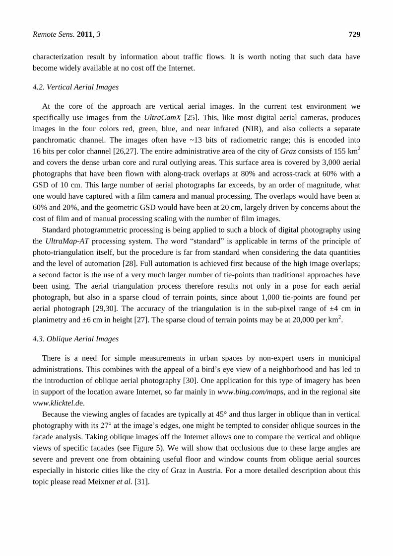
Because the viewing angles of facades are typically at 45° and thus larger in oblique than in vertical
photography with its 27° at the image’s edges, one might be tempted to consider oblique sources in the
facade analysis. Taking oblique images off the Internet allows one to compare the vertical and oblique
views of specific facades (see Figure 5). We will show that occlusions due to these large angles are
severe and prevent one from obtaining useful floor and window counts from oblique aerial sources
especially in historic cities like the city of Graz in Austria. For a more detailed description about this
topic please read Meixner et al. [31].
Remote Sens. 2011, 3
730
Figure 5. Oblique aerial image at 45° look angle taken from Bing Maps (left); Vertical
aerial image obtained from UltraCamX at a look angle of 27° (right). The marked sections
in the original image segments (above) have been rectified (below).
4.4. Derived from Vertical Aerial Images: DSM and DTM Data
The Digital Surface Model (DSM) is created by ―dense matching‖. The input consists of the
triangulated aerial photographs. In this process, one develops point clouds from subsets of the
overlapping images and then merge (fuse) the separately developed point clouds of a given area. The
process is described by Klaus in [21]. For property classification, the elevation data are considered as
input. Data used in our property-related experiments have been obtained from work at Microsoft
Graz [27]. The conversion of the surface model DSM into a Bald Earth Digital Terrain Model (DTM)
is a post-process of dense matching and has been described by Zebedin et al. [32].
The postings of the DSM and DTM are at 2 pixel intervals, and result in about 25 million points
per km2, far denser than traditional photogrammetry rules would support. However, because the
overlaps of 80% and 60% result in 10 images per ground point, one is observing a type of
―super-resolution‖ that supports a very dense sampling of terrain points. It has been shown that the
vertical accuracy of such DSMs is in the range of about ±0.5 pixels [33], provided the surface is
well defined.
4.5. Derived from Vertical Aerial Images: True Orthophoto
The DSM is the reference surface onto which each aerial photograph is projected. The DSM and its
associated photographic texture are then projected orthogonally into the XY-plane and result in what is
denoted as a ―true‖ orthophoto. In this data product, the buildings are only shown by their roofs, not
however by their facades. Given the overlaps of the source images, the orthophoto can be constructed
in such a way that all occlusions are avoided. Image detail in the orthophoto is therefore taken from
multiple aerial images in a manner that would not be customary in traditional film-based
orthophotography.
Remote Sens. 2011, 3
731
In the current context, the true orthophoto is an auxiliary tool for visual inspection of intermediate
results. One could also use traditional orthophotos that have been projected not onto the DSM but onto
the Bald Earth DTM instead. The traditional orthophoto would, however, show far less concurrence
with the cadastral map. For further details about this method see Zebedin et al. [32] and
Oda et al. [34]. Another possibility of generating true orthophotos is to use a fusion step where
massive redundant image data is transformed to a common (ortho) view and processed with
e.g., variational methods as described by Zach et al. [35] or Kluckner et al. [36].
4.6. Derived from Aerial Images: Classification into Segmented Images
Any urban area of interest can be covered by multiple color aerial images. These can be subjected to
an automated classification to develop information layers about the area. We consider these as input
for our characterization procedures. The classification approach used here has been described by
Gruber-Geymayer et al. [37] and Zebedin et al. [32]. However, classification and segmentation
methods are topics of intense research. For example Kluckner et al. [38] have proposed alternative
novel methods with good results specifically interpreting urban scenes imaged by the UltraCam digital
aerial camera.
Standard classifications of 4-channel digital aerial photography typically lead to seven separate data
layers: buildings; grass; trees; sealed surfaces; bare earth; water; other objects (―unclassified‖). The
unclassified areas may show lamp posts, cars, buses, people, etc. Gruber-Geymayer et al. [39] report
typical classification accuracies in the range of 90%: this means that a 10% error is being made either
by assigning a class in error or not assigning any class.
4.7. Cadaster for Property Boundaries
Since a ―property boundary‖ is a legal concept, it is not typically visible in the field and from the
air. Also image segmentation algorithms cannot properly distinguish between buildings when they are
physically attached to one another. It will be the rare exception that attached buildings can be separated
from aerial imagery, for example if the roof styles differ, building heights vary or the colors of the
roofing tiles differ. Obviously then one needs to introduce the cadastral map.
Cadastral information has a long history that is reflected in a need to consider its national
circumstances and historical development to avoid negative surprises. The accuracy and the historical
development of the Austrian land register can be considered to be at a rather highly developed level
not found in many countries.
For the study area in the city of Graz we have cadastral data available from the year 2008, provided
by the Austrian Federal Mapping Agency Bundesamt für Eich- und Vermessungswesen (BEV, see
Figure 4). The cadastral information addresses property boundaries, and not necessarily building
footprints, although such building data may be provided from the cadastral sources, albeit with some
uncertainty and oftentimes somewhat dated. The cadastral accuracy is quoted at ±10 cm which is
equivalent to the range of the aerial photography’s pixel size and thus sufficient for the purpose of
characterizing real properties [40].
Remote Sens. 2011, 3
732
4.8. Optional Street Network and Address Data
Car navigation has been the driver for the global development of digital street maps. They also
support location awareness of Internet searches. Since the vector format of street maps is not available
free of charge, it is at times re-engineered from the raster display off the Internet [41]. The example for
the Graz study site, in Figures 3 and 4, illustrates the scarcity of street map. And yet it can add unique
information about traffic and traffic-related property-characteristics. Of course the street maps would
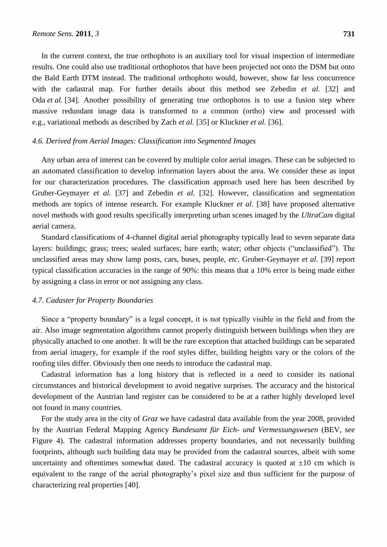
take on a much elevated importance if there was no cadastral data (Figure 6).
Figure 6. Street layer for the area in Figure 3 taken off the Internet search system Bing
Maps (Microsoft, November 2009). The raster GSD has been resampled to fit the aerial
imagery sources at a GSD of 10 cm. To the right is a ―hybrid‖ view of the street layer
superimposed onto the orthophoto.
Address information is encoded in the form of a point and its geographic latitude and longitude.
This is valuable when attaching alphanumeric information to a property. Again, this source is of
elevated importance when one needs to cope with the absence of a cadaster. Between the street map,
address data and the orthophoto, one will have to devise a strategy for approximating cadastral
information.
4.9. Comments
All image-based source data for the proposed property work are the result of extensive computation
and data processing, some of which constitutes the outcome of considerable recent innovations, such
as dense image matching and fully automated aerial triangulation. However, none of this processing is
specific to the property characterization; therefore we do not address it in this paper.
The growing diversity of Geodata sources has recently been discussed by Blumenthal [24] with
respect to efforts made at Google. Two innovative phenomena stand out: crowd sourced imagery and
motion traces. Both may have an impact on the property characterization as such data becomes
increasingly more available. The detail from crowd sourced imagery (also denoted as Community
Photo Collections CPC) will probably exceed by a level of magnitude that of aerial imagery. The
Remote Sens. 2011, 3
733
developments in this domain hold great promise [42-44]. Even new words are being introduced to deal
with these changes, for example ―neo-geographer‖ [45]. A separate novel type of Geodata is the
motion trace offering the option of modeling noise from traffic.
The Graz study area is 400 m × 400 m and contains 216 buildings situated on 321 parcels. This
suggests that multiple parcels may combine into a single property.
5. Assembling Data per Property
5.1. Chamfer-Matching the Cadastral Map with the Building Classification
Most cadastral maps, including the Austrian cadastre, basically present a 2D data base and ignore
the 3rd dimension. This causes issues when relating the cadastral data to the aerial photography and its
inherently 3D data products. Co-registration therefore may be accomplished using the 2D building
classification and a match between this and the 2D-cadastral map. Once this co-registration is
achieved, the cadastral data are also geometrically aligned with all the orthophoto and other
photo-derived data sets.
A 2-step process serves to match the 2D cadastral vector map (in its own coordinate system) and the
2D orthophoto (with its different coordinate reference). In a first step, the cadastral point coordinates
simply get converted from their Gauss-Krüger M34 values to the building classification’s Universal
Transverse Mercator UTM system. In an ideal world, this would solve the registration problem.
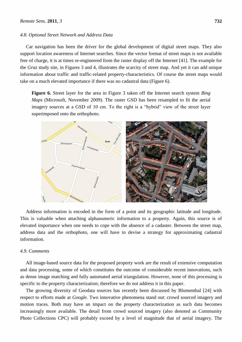
However, it does not, as illustrated in Figure 7 (left).
Figure 7. Overlaying the cadastral map over the orthophoto will leave some small errors
that need to be found and removed. Left is the overlay after step 1 of the registration,
namely the coordinate transformation from the Gauss-Krüger to the UTM system. To the
right is the result after a Chamfer-match has been applied. The area is a segment of the
study area in Figure 3.
A second step is thus needed to achieve a fine alignment of the cadastre and the building
classification. This is because small projection errors exist in the range of a few pixels (some
tens of cm).
Remote Sens. 2011, 3
734
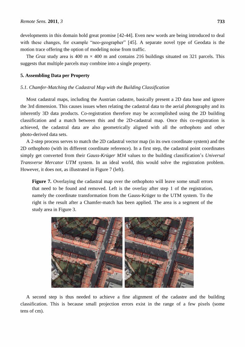
This adjustment is accomplished by a so-called Chamfer-match, here implemented after
Borgefors [46]. The algorithm converts the vector image of the cadastral map into a raster image and
assigns a grey value to each pixel as a function of the distance from the nearest vector. This is denoted
as a distance image. The resulting raster image from the cadastre is shown in Figure 8. In a similar
fashion, the building classification is transformed into an edge image. Chamfer-matching now employs
these two computed auxiliary raster images by overlapping them to find small geometric changes to
make them fit optimally. In our case this linear alignment is computed for the entire image patch. For
this data set no non-linear misalignments like shearing or rotation occur, they are all solved in the first
step. Figure 7 (right) supports the conclusion that discrepancies have been reduced from their previous
±7 pixels down to a mere ±2 pixels (GSD = 10 cm).
Figure 8. Cadastral raster image in the format of a computed distance transform
image (left) and the edges of the segmented image (right), both used as an input to the
Chamfer-match after Borgefors [46].
5.2. Class-Specific Segmentation per Individual Properties
The image segmentation result has the same coordinate system as the orthophoto. Therefore the
cadastral map can be used directly to cut a classification map into data per property. Figure 9 illustrates
the result.
An evaluation of the automated segmentation is based on manually developed ground truth. For the
example of the building information, the result confirms that the classification approach implemented
by Gruber-Geymayer et al. [37] and Zebedin et al. [32] delivers an accuracy of 90%. Classification
uncertainties are caused by mismatches between cadastral line work and the building outlines when a
cadastral boundary line coincides with a building facade. We may find facade details such as
balconies, or roof extensions in the form of eaves that violate cadastral delineations. Having the
cadaster available offers one the option of changing the segmentation and classification along building
and property boundaries.
Remote Sens. 2011, 3
735
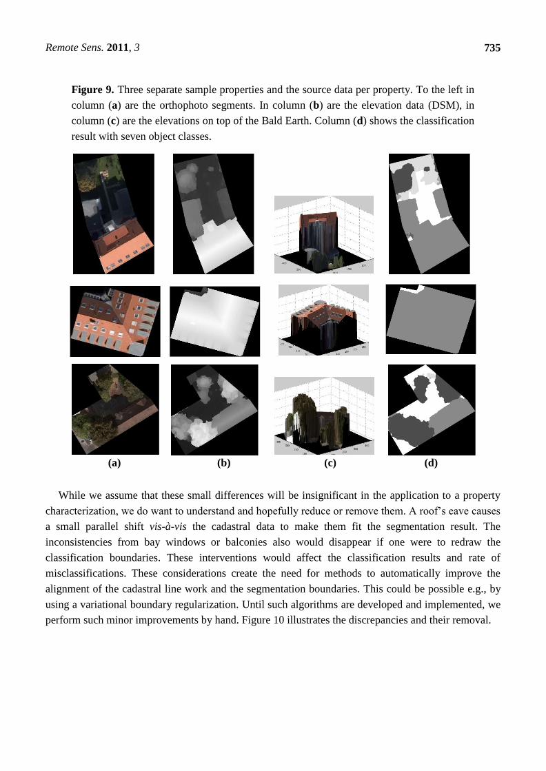
Figure 9. Three separate sample properties and the source data per property. To the left in
column (a) are the orthophoto segments. In column (b) are the elevation data (DSM), in
column (c) are the elevations on top of the Bald Earth. Column (d) shows the classification
result with seven object classes.
(a) (b) (c) (d)
While we assume that these small differences will be insignificant in the application to a property
characterization, we do want to understand and hopefully reduce or remove them. A roof’s eave causes
a small parallel shift vis-à-vis the cadastral data to make them fit the segmentation result. The
inconsistencies from bay windows or balconies also would disappear if one were to redraw the
classification boundaries. These interventions would affect the classification results and rate of
misclassifications. These considerations create the need for methods to automatically improve the
alignment of the cadastral line work and the segmentation boundaries. This could be possible e.g., by
using a variational boundary regularization. Until such algorithms are developed and implemented, we
perform such minor improvements by hand. Figure 10 illustrates the discrepancies and their removal.
Remote Sens. 2011, 3
736
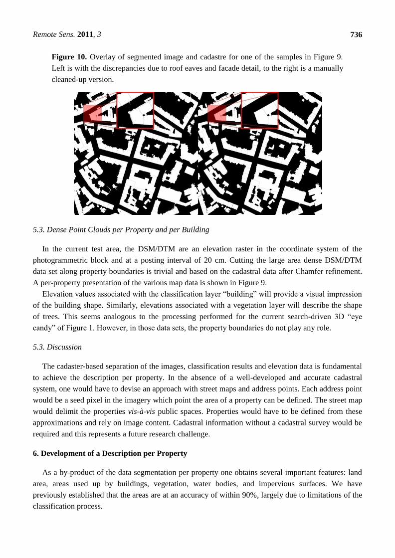
Figure 10. Overlay of segmented image and cadastre for one of the samples in Figure 9.
Left is with the discrepancies due to roof eaves and facade detail, to the right is a manually
cleaned-up version.
5.3. Dense Point Clouds per Property and per Building
In the current test area, the DSM/DTM are an elevation raster in the coordinate system of the
photogrammetric block and at a posting interval of 20 cm. Cutting the large area dense DSM/DTM
data set along property boundaries is trivial and based on the cadastral data after Chamfer refinement.
A per-property presentation of the various map data is shown in Figure 9.
Elevation values associated with the classification layer ―building‖ will provide a visual impression
of the building shape. Similarly, elevations associated with a vegetation layer will describe the shape
of trees. This seems analogous to the processing performed for the current search-driven 3D ―eye
candy‖ of Figure 1. However, in those data sets, the property boundaries do not play any role.
5.3. Discussion
The cadaster-based separation of the images, classification results and elevation data is fundamental
to achieve the description per property. In the absence of a well-developed and accurate cadastral
system, one would have to devise an approach with street maps and address points. Each address point
would be a seed pixel in the imagery which point the area of a property can be defined. The street map
would delimit the properties vis-à-vis public spaces. Properties would have to be defined from these
approximations and rely on image content. Cadastral information without a cadastral survey would be
required and this represents a future research challenge.
6. Development of a Description per Property
As a by-product of the data segmentation per property one obtains several important features: land
area, areas used up by buildings, vegetation, water bodies, and impervious surfaces. We have
previously established that the areas are at an accuracy of within 90%, largely due to limitations of the
classification process.
Remote Sens. 2011, 3
737
By introducing the 3rd dimension in the form of the dense point cloud, one adds relevant property
information and improves the accuracy of area measurements previously obtained in the 2D
classification. An overriding role is associated with buildings; therefore they are the focus of our initial
efforts. Going through each property, we add descriptive information about its buildings.
6.1. Finding the Footprint of Facades in 2D
(a) Vectorizing the Building Contour
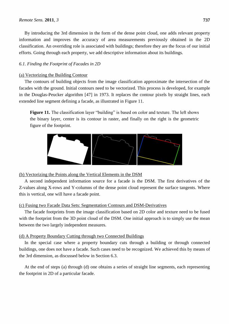
The contours of building objects from the image classification approximate the intersection of the
facades with the ground. Initial contours need to be vectorized. This process is developed, for example
in the Douglas-Peucker algorithm [47] in 1973. It replaces the contour pixels by straight lines, each
extended line segment defining a facade, as illustrated in Figure 11.
Figure 11. The classification layer ―building‖ is based on color and texture. The left shows
the binary layer, center is its contour in raster, and finally on the right is the geometric
figure of the footprint.
(b) Vectorizing the Points along the Vertical Elements in the DSM
A second independent information source for a facade is the DSM. The first derivatives of the
Z-values along X-rows and Y-columns of the dense point cloud represent the surface tangents. Where
this is vertical, one will have a facade point.
(c) Fusing two Facade Data Sets: Segmentation Contours and DSM-Derivatives
The facade footprints from the image classification based on 2D color and texture need to be fused
with the footprint from the 3D point cloud of the DSM. One initial approach is to simply use the mean
between the two largely independent measures.
(d) A Property Boundary Cutting through two Connected Buildings
In the special case where a property boundary cuts through a building or through connected
buildings, one does not have a facade. Such cases need to be recognized. We achieved this by means of
the 3rd dimension, as discussed below in Section 6.3.
At the end of steps (a) through (d) one obtains a series of straight line segments, each representing
the footprint in 2D of a particular facade.
Remote Sens. 2011, 3
738
6.2. Decomposing a Building into Separate Building Objects
At issue is the number of a building’s facades and thus the building’s complexity. The simplest
building will have four facades at right angles. However, there is no limit to the complexity of building
shapes and thus of the number of facades, and also of the angles formed between adjacent facades.
The option exists to fit the pattern of facade footprints into a series of predefined shapes of
(rectangular) building footprints. In the process one hopes to develop a set of separate non-overlapping
basic building objects or ―sub-buildings‖. This could be obtained via a segmentation of the building
footprint. However, one could also review the roof shapes. Having more than one local maximum in
the roof height is an indication that the single building has a complex shape and should be segmented
into multiple building objects or sub-buildings. This is of course not the case for all roof types e.g.,
gabled roofs.
6.3. Adding the 3rd Dimension to the Facade
Along the footprints of the facade one finds elevation values in the DSM. These attach a 3rd
dimension to the facade. The simplest facade shape is a rectangle. Depending on the shape of the roof,
a facade could also have a complex shape. Should the elevations change along the facade footprint, we
could be facing a sloping ground or a varying roof line, or a combination of both. The slope of the
ground is known from the DTM. Variations of the roof line are available from the difference between
the DSM and the DTM. For use as a property descriptor, one might be satisfied with a single elevation
value for each facade. Therefore we initially associate a vertical rectangle to each facade.
We have previously mentioned connected buildings and a property line cutting through buildings,
leading to virtual facades. These can be identified via a look at the dense point cloud. The elevation
values above the Bald Earth along a facade footprint will be zero at one side of the footprint. If they
are not, then this facade will be marked as ―virtual‖.
6.4. From the Facade to the Height of a Building and Its Roof
As a minimum, we want to use two elevations values for each building: the height of the roof line
and the height of the roof’s highest point. But given that a building has multiple facades, possibly built
on a sloping ground and does not have a single roof line, one is faced with a more complex issue than
expected. For simplicity, we initially average the multiple facade heights to a single value, and we
define the roof height as the elevation difference between the highest point on the roof and the
computed facade height.
6.5. Occlusions
Parts of buildings may be occluded by vegetation, other buildings or other objects such as cars or
people. Any detailing of building information must be built with an understanding of the existence of
occlusions. We see two approaches to deal with this issue. The first is the reliance on the known
incidence angles defined by the camera station and neighborhood facade footprints. As one processes
overlapping images and obtains different results, these differences themselves can indicate the effect of
occlusions and cause a second look to be given to identify an occlusion. A second approach is a
Remote Sens. 2011, 3
739
geometric process using the facade footprints, the DSM and the camera station. Occlusions get
computed by Z-buffering or ray tracing.
7. Counting Floors and Windows
7.1. Vertical Aerial Photography
We proceed from the basic building description to an analysis of the facades. Work on building
facades would intuitively build on street level photography or at least oblique aerial imagery.
However, our interest is in understanding how well one can study facades in (cost free) vertical aerial
photography. The facade detail of interest is a floor count, a window count and a description of the
window’s location and size.
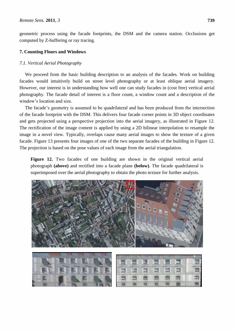
The facade’s geometry is assumed to be quadrilateral and has been produced from the intersection
of the facade footprint with the DSM. This delivers four facade corner points in 3D object coordinates
and gets projected using a perspective projection into the aerial imagery, as illustrated in Figure 12.
The rectification of the image content is applied by using a 2D bilinear interpolation to resample the
image in a novel view. Typically, overlaps cause many aerial images to show the texture of a given
facade. Figure 13 presents four images of one of the two separate facades of the building in Figure 12.
The projection is based on the pose values of each image from the aerial triangulation.
Figure 12. Two facades of one building are shown in the original vertical aerial
photograph (above) and rectified into a facade plane (below). The facade quadrilateral is
superimposed over the aerial photography to obtain the photo texture for further analysis.
Remote Sens. 2011, 3
740
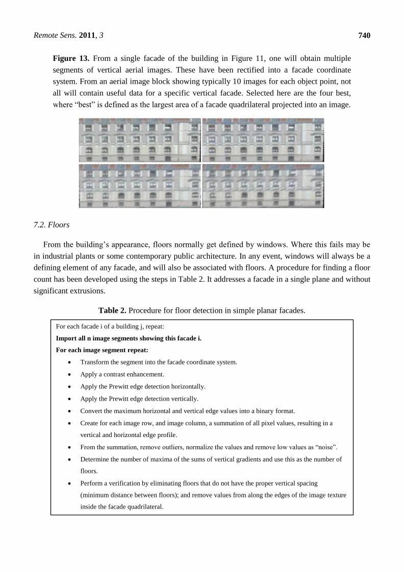
Figure 13. From a single facade of the building in Figure 11, one will obtain multiple
segments of vertical aerial images. These have been rectified into a facade coordinate
system. From an aerial image block showing typically 10 images for each object point, not
all will contain useful data for a specific vertical facade. Selected here are the four best,
where ―best‖ is defined as the largest area of a facade quadrilateral projected into an image.
7.2. Floors
From the building’s appearance, floors normally get defined by windows. Where this fails may be
in industrial plants or some contemporary public architecture. In any event, windows will always be a
defining element of any facade, and will also be associated with floors. A procedure for finding a floor
count has been developed using the steps in Table 2. It addresses a facade in a single plane and without
significant extrusions.
Table 2. Procedure for floor detection in simple planar facades.
For each facade i of a building j, repeat:
Import all n image segments showing this facade i.
For each image segment repeat:
Transform the segment into the facade coordinate system.
Apply a contrast enhancement.
Apply the Prewitt edge detection horizontally.
Apply the Prewitt edge detection vertically.
Convert the maximum horizontal and vertical edge values into a binary format.
Create for each image row, and image column, a summation of all pixel values, resulting in a
vertical and horizontal edge profile.
From the summation, remove outliers, normalize the values and remove low values as ―noise‖.
Determine the number of maxima of the sums of vertical gradients and use this as the number of
floors.
Perform a verification by eliminating floors that do not have the proper vertical spacing
(minimum distance between floors); and remove values from along the edges of the image texture
inside the facade quadrilateral.
Remote Sens. 2011, 3
741
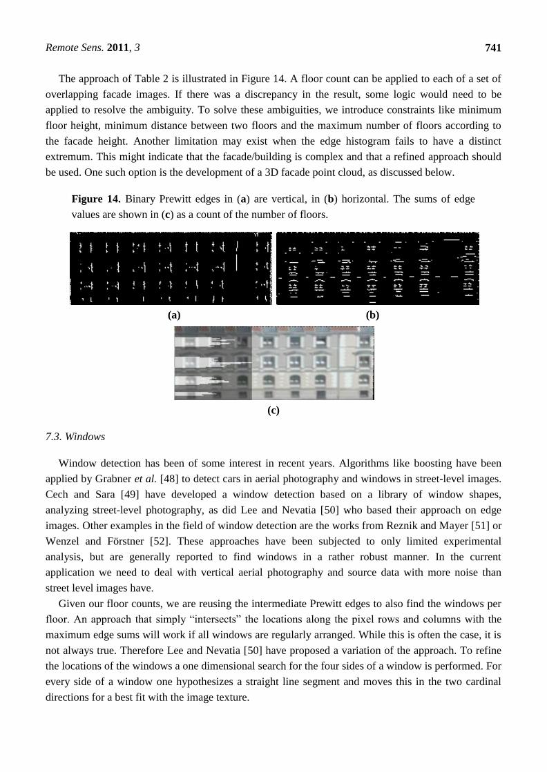
The approach of Table 2 is illustrated in Figure 14. A floor count can be applied to each of a set of
overlapping facade images. If there was a discrepancy in the result, some logic would need to be
applied to resolve the ambiguity. To solve these ambiguities, we introduce constraints like minimum
floor height, minimum distance between two floors and the maximum number of floors according to
the facade height. Another limitation may exist when the edge histogram fails to have a distinct
extremum. This might indicate that the facade/building is complex and that a refined approach should
be used. One such option is the development of a 3D facade point cloud, as discussed below.
Figure 14. Binary Prewitt edges in (a) are vertical, in (b) horizontal. The sums of edge
values are shown in (c) as a count of the number of floors.
(a) (b)
(c)
7.3. Windows
Window detection has been of some interest in recent years. Algorithms like boosting have been
applied by Grabner et al. [48] to detect cars in aerial photography and windows in street-level images.
Cech and Sara [49] have developed a window detection based on a library of window shapes,
analyzing street-level photography, as did Lee and Nevatia [50] who based their approach on edge
images. Other examples in the field of window detection are the works from Reznik and Mayer [51] or
Wenzel and Förstner [52]. These approaches have been subjected to only limited experimental
analysis, but are generally reported to find windows in a rather robust manner. In the current
application we need to deal with vertical aerial photography and source data with more noise than
street level images have.
Given our floor counts, we are reusing the intermediate Prewitt edges to also find the windows per
floor. An approach that simply ―intersects‖ the locations along the pixel rows and columns with the
maximum edge sums will work if all windows are regularly arranged. While this is often the case, it is
not always true. Therefore Lee and Nevatia [50] have proposed a variation of the approach. To refine
the locations of the windows a one dimensional search for the four sides of a window is performed. For
every side of a window one hypothesizes a straight line segment and moves this in the two cardinal
directions for a best fit with the image texture.
Remote Sens. 2011, 3
742
We find this method applicable to images with lower resolution, as is the case in facades imaged in
vertical aerial photography. Also not only rectangular windows but other window designs can be
automatically detected as well and rather quickly, without training the program in advance. The
window count is applicable in each image segment of a given facade, separately. Or one might want to
merge the edge data sets and apply single window detection to the sum of all edges. A comparison of
the various different methods for window detection is pending and will be subject of ongoing work.
7.4. Multiple Facades per Building
We may find different floor numbers from the multiple facades of one building. It is possible that a
building has different floor counts on a sloping terrain. Since the Bald Earth as well as the slope of a
building footprint is known, this must enter into the floor count.
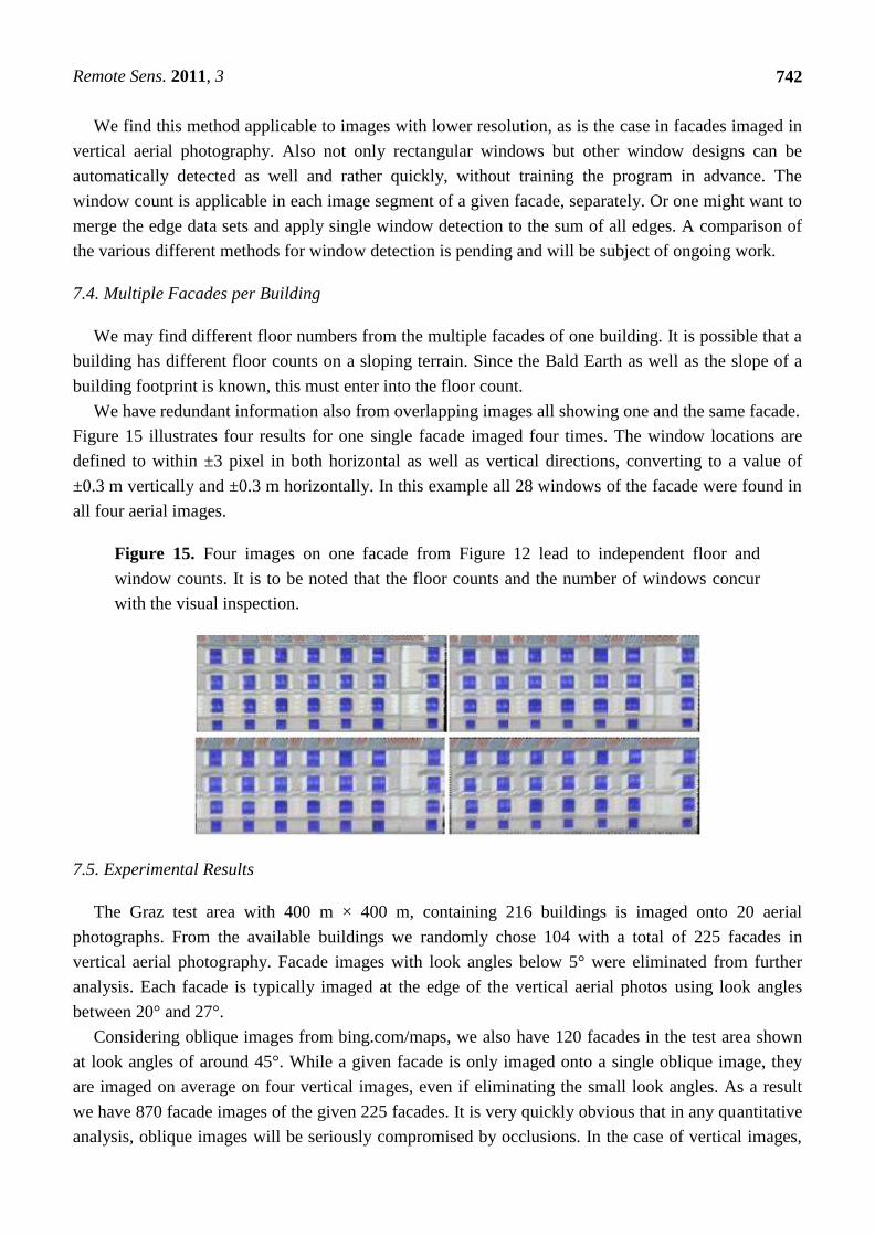
We have redundant information also from overlapping images all showing one and the same facade.
Figure 15 illustrates four results for one single facade imaged four times. The window locations are
defined to within ±3 pixel in both horizontal as well as vertical directions, converting to a value of
±0.3 m vertically and ±0.3 m horizontally. In this example all 28 windows of the facade were found in
all four aerial images.
Figure 15. Four images on one facade from Figure 12 lead to independent floor and
window counts. It is to be noted that the floor counts and the number of windows concur
with the visual inspection.
7.5. Experimental Results
The Graz test area with 400 m × 400 m, containing 216 buildings is imaged onto 20 aerial
photographs. From the available buildings we randomly chose 104 with a total of 225 facades in
vertical aerial photography. Facade images with look angles below 5° were eliminated from further
analysis. Each facade is typically imaged at the edge of the vertical aerial photos using look angles
between 20° and 27°.
Considering oblique images from bing.com/maps, we also have 120 facades in the test area shown
at look angles of around 45°. While a given facade is only imaged onto a single oblique image, they
are imaged on average on four vertical images, even if eliminating the small look angles. As a result
we have 870 facade images of the given 225 facades. It is very quickly obvious that in any quantitative
analysis, oblique images will be seriously compromised by occlusions. In the case of vertical images,
Remote Sens. 2011, 3
743
occlusions are reduced as the look angles become steeper. And since we operate with four or more
vertical images of each facade, we can exploit the redundancy to find a most likely correct floor and
window count.
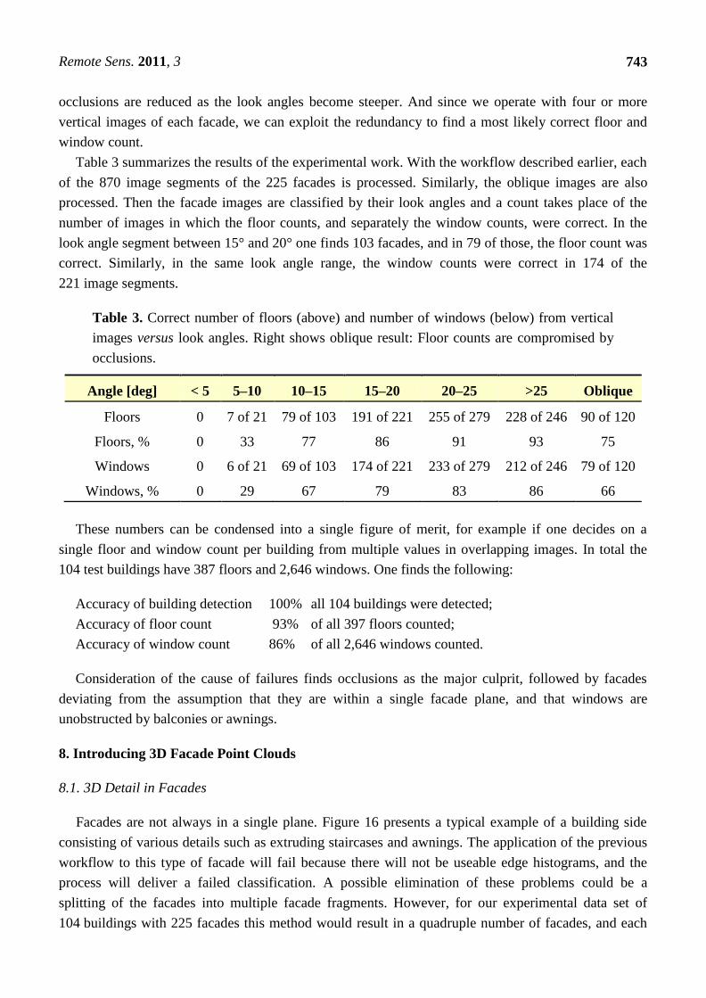
Table 3 summarizes the results of the experimental work. With the workflow described earlier, each
of the 870 image segments of the 225 facades is processed. Similarly, the oblique images are also
processed. Then the facade images are classified by their look angles and a count takes place of the
number of images in which the floor counts, and separately the window counts, were correct. In the
look angle segment between 15° and 20° one finds 103 facades, and in 79 of those, the floor count was
correct. Similarly, in the same look angle range, the window counts were correct in 174 of the
221 image segments.
Table 3. Correct number of floors (above) and number of windows (below) from vertical
images versus look angles. Right shows oblique result: Floor counts are compromised by
occlusions.
These numbers can be condensed into a single figure of merit, for example if one decides on a
single floor and window count per building from multiple values in overlapping images. In total the
104 test buildings have 387 floors and 2,646 windows. One finds the following:
Accuracy of building detection 100% all 104 buildings were detected;
Accuracy of floor count 93% of all 397 floors counted;
Accuracy of window count 86% of all 2,646 windows counted.
Consideration of the cause of failures finds occlusions as the major culprit, followed by facades
deviating from the assumption that they are within a single facade plane, and that windows are
unobstructed by balconies or awnings.
8. Introducing 3D Facade Point Clouds
8.1. 3D Detail in Facades
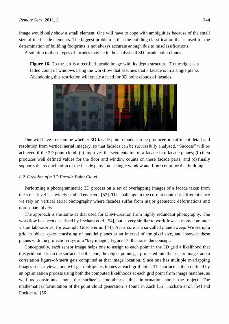
Facades are not always in a single plane. Figure 16 presents a typical example of a building side
consisting of various details such as extruding staircases and awnings. The application of the previous
workflow to this type of facade will fail because there will not be useable edge histograms, and the
process will deliver a failed classification. A possible elimination of these problems could be a
splitting of the facades into multiple facade fragments. However, for our experimental data set of
104 buildings with 225 facades this method would result in a quadruple number of facades, and each
Angle [deg] < 5 5–10 10–15 15–20 20–25 >25 Oblique
Floors 0 7 of 21 79 of 103 191 of 221 255 of 279 228 of 246 90 of 120
Floors, % 0 33 77 86 91 93 75
Windows 0 6 of 21 69 of 103 174 of 221 233 of 279 212 of 246 79 of 120
Windows, % 0 29 67 79 83 86 66
Remote Sens. 2011, 3
744
image would only show a small element. One will have to cope with ambiguities because of the small
size of the facade elements. The biggest problem is that the building classification that is used for the
determination of building footprints is not always accurate enough due to misclassifications.
A solution to these types of facades may be in the analysis of 3D facade point clouds.
Figure 16. To the left is a rectified facade image with its depth structure. To the right is a
failed count of windows using the workflow that assumes that a facade is in a single plane.
Abandoning this restriction will create a need for 3D point clouds of facades.
One will have to examine whether 3D facade point clouds can be produced in sufficient detail and
resolution from vertical aerial imagery, so that facades can be successfully analyzed. ―Success‖ will be
achieved if the 3D point cloud: (a) improves the segmentation of a facade into facade planes; (b) then
produces well defined values for the floor and window counts on these facade parts; and (c) finally
supports the reconciliation of the facade parts into a single window and floor count for that building.
8.2. Creation of a 3D Facade Point Cloud
Performing a photogrammetric 3D process on a set of overlapping images of a facade taken from
the street level is a widely studied endeavor [53]. The challenge in the current context is different since
we rely on vertical aerial photography where facades suffer from major geometric deformations and
non-square pixels.
The approach is the same as that used for DSM-creation from highly redundant photography. The
workflow has been described by Irschara et al. [54], but is very similar to workflows at many computer
vision laboratories, for example Gösele et al. [44]. At its core is a so-called plane sweep. We set up a
grid in object space consisting of parallel planes at an interval of the pixel size, and intersect these
planes with the projection rays of a ―key image‖. Figure 17 illustrates the concept.
Conceptually, each sensor image helps one to assign to each point in the 3D grid a likelihood that
this grid point is on the surface. To this end, the object points get projected into the sensor image, and a
correlation figure-of-merit gets computed at that image location. Since one has multiple overlapping
images sensor views, one will get multiple estimates at each grid point. The surface is then defined by
an optimization process using both the computed likelihoods at each grid point from image matches, as
well as constraints about the surface’s smoothness, thus information about the object. The
mathematical formulation of the point cloud generation is found in Zach [55], Irschara et al. [54] and
Pock et al. [56].
Remote Sens. 2011, 3
745
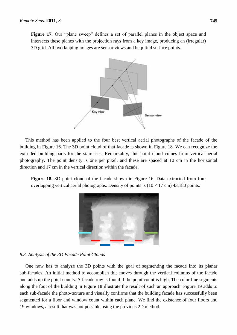
Figure 17. Our ―plane sweep‖ defines a set of parallel planes in the object space and
intersects these planes with the projection rays from a key image, producing an (irregular)
3D grid. All overlapping images are sensor views and help find surface points.
This method has been applied to the four best vertical aerial photographs of the facade of the
building in Figure 16. The 3D point cloud of that facade is shown in Figure 18. We can recognize the
extruded building parts for the staircases. Remarkably, this point cloud comes from vertical aerial
photography. The point density is one per pixel, and these are spaced at 10 cm in the horizontal
direction and 17 cm in the vertical direction within the facade.
Figure 18. 3D point cloud of the facade shown in Figure 16. Data extracted from four
overlapping vertical aerial photographs. Density of points is (10 × 17 cm) 43,180 points.
8.3. Analysis of the 3D Facade Point Clouds
One now has to analyze the 3D points with the goal of segmenting the facade into its planar
sub-facades. An initial method to accomplish this moves through the vertical columns of the facade
and adds up the point counts. A facade row is found if the point count is high. The color line segments
along the foot of the building in Figure 18 illustrate the result of such an approach. Figure 19 adds to
each sub-facade the photo-texture and visually confirms that the building facade has successfully been
segmented for a floor and window count within each plane. We find the existence of four floors and
19 windows, a result that was not possible using the previous 2D method.
Remote Sens. 2011, 3
746
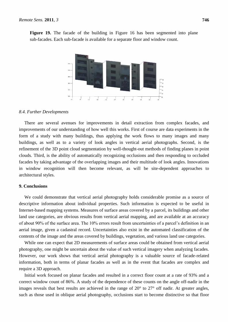
Figure 19. The facade of the building in Figure 16 has been segmented into plane
sub-facades. Each sub-facade is available for a separate floor and window count.
8.4. Further Developments
There are several avenues for improvements in detail extraction from complex facades, and
improvements of our understanding of how well this works. First of course are data experiments in the
form of a study with many buildings, thus applying the work flows to many images and many
buildings, as well as to a variety of look angles in vertical aerial photographs. Second, is the
refinement of the 3D point cloud segmentation by well-thought-out methods of finding planes in point
clouds. Third, is the ability of automatically recognizing occlusions and then responding to occluded
facades by taking advantage of the overlapping images and their multitude of look angles. Innovations
in window recognition will then become relevant, as will be site-dependent approaches to
architectural styles.
9. Conclusions
We could demonstrate that vertical aerial photography holds considerable promise as a source of
descriptive information about individual properties. Such information is expected to be useful in
Internet-based mapping systems. Measures of surface areas covered by a parcel, its buildings and other
land use categories, are obvious results from vertical aerial mapping, and are available at an accuracy
of about 90% of the surface area. The 10% errors result from uncertainties of a parcel’s definition in an
aerial image, given a cadastral record. Uncertainties also exist in the automated classification of the
contents of the image and the areas covered by buildings, vegetation, and various land use categories.
While one can expect that 2D measurements of surface areas could be obtained from vertical aerial
photography, one might be uncertain about the value of such vertical imagery when analyzing facades.
However, our work shows that vertical aerial photography is a valuable source of facade-related
information, both in terms of planar facades as well as in the event that facades are complex and
require a 3D approach.
Initial work focused on planar facades and resulted in a correct floor count at a rate of 93% and a
correct window count of 86%. A study of the dependence of these counts on the angle off-nadir in the
images reveals that best results are achieved in the range of 20° to 27° off nadir. At greater angles,
such as those used in oblique aerial photography, occlusions start to become distinctive so that floor
Remote Sens. 2011, 3
747
and window counts fail. Such counts will also fail if a facade is complex, yet the analysis method is
unaware of that complexity. One needs then to consider the 3D shape of building facades, for example
with extruding stair cases, balconies, awnings. We explain in this paper an approach based on 3D
clouds of facade surface points, all extracted from overlapping vertical images. We have explained the
approach by example and will have to embark on a systematic study of its performance with many
buildings and imaging configurations. It seems not only important to test the work flow on many
buildings, but also that the buildings represent a variety of sizes and styles and come from different
regions (cities and rural areas) and parts of the world.
The complexity of describing buildings is immense and much work remains to be done. One needs
to obtain a good understanding of the accuracy and reliability of a building’s key numbers in all cases.
One needs to solve the problems faced when: parts of a building are occluded; the geometric resolution
of the source data varies; buildings deviate from expected shapes in the event of add-ons and of
complex footprints and roof shapes; the building’s use is mixed and an industrial use leads to
windowless facades; cadastral detail contradicts image detail, etc.
At issue in this paper is of course also the motivation for the development of descriptive data about
real properties (or real estate). An initial driver to embark on this research has been the disappointment
when faced with the lack of detailed information about objects shown in Internet-maps on Google
Earth or BingMaps, and the expectation that such information could be available at very little extra
cost from image sources in existence for other purposes. Were such detailed information to exist, it
could be useful in location-based decisions of both commercial and public interest, and in a better
administration of municipal resources. The more thorough use of vertical aerial photography is
globally expected to be augmented by significant efforts to conflate various 2D Geodata sources, to be
added to business and private address data bases and parcel data, and by the start of massive
collections of GNSS and cellular traces. This is separate from an increasing interest in human scale
details of urban data that is reflected initially in the form of street-side imagery taken by moving
vehicles, but in the long run is expected to come from Community-Photo-Collections (CPC), such as
those in FLICKR. This in turn will be part of a broader concept of user-generated content (UGC).
Much of Internet-mapping is currently a result of the search application. However, one may be able
to see on the horizon an advent of spatial information as an integral part of the evolution of the
Internet-of-Things (―IoT‖) and of Ambient Intelligence (―AmI‖), as projected by Weiser [19] or
O’Reilly and Batelle [18].
Acknowledgements
The aerial images and their data products DTM, DSM, orthophotos and segmented land use classes
were provided with the support of Barbara Gruber-Geymayer and Michael Gruber at
Microsoft-Photogrammetry in Graz. Our colleagues Michael Donoser, Stefan Kluckner and Arnold
Irschara at the Institute for Computer Graphics and Vision were and continue to be a great inspiration
for new algorithms, software and knowledge.
Remote Sens. 2011, 3
748
References
1. Gartner, G.; Rehrl K. Location Based Services and TeleCartography II: From Sensor Fusion to
Context Models; Lecture Notes in Geoinformation and Cartography; In Proceedings of 5th
International Conference on Location Based Services and TeleCartography, Salzburg, Austria,
26–28 November 2008; Springer-Verlag: Berlin/Heidelberg, Germany, 2009; Volume 29, p. 456.
2. Leberl, F. Die automatische Photogrammetrie für das Microsoft Virtual Earth System. In
Proceedings of 14th Internationale Geodätische Woche, Obergurgl, Austria, 11–17 February
2007; pp. 200-208.
3. Leberl, F.; Gruber, M.; Ponticelli, M.; Bernögger, S. Ultracamx, the Large Format Digital Aerial
Camera System by Vexcel Imaging/Microsoft. In Proceedings of XXIst ISPRS, Beijing, China,
3–11 July 2008; In The International Archives of the Photogrammetry, Remote Sensing and
Spatial Information Sciences, ISPRS: Vienna, Austria, 2008; Volume 37, pp. 665-670.
4. Leberl, F.; Gruber, M. Ortsbewusstsein im Internet—von 2-dimensionalen Navigationshilfen zur
3-dimensionalen Mixed Reality. In Proceedings of 15 Internationale Geodätische Woche
Obergurgl 2009, Obergurgl, Austria, 8–14 February 2009; pp. 67-79.
5. Leberl, F.; Gruber, M. 3D-Models of the Human Habitat for the Internet. In Proceedings of
Visigrapp 2009, Lisbon, Portugal, 5–8 February 2009; INSTCC-Portugal: Lisbon, Portugal, 2009;
pp. 7-15.
6. Paul, R. Microsoft Launches Virtual Earth 3D to Try and Take on Google Earth. 7 November
2006. Available online: http://www.earthtimes.org/articles/show/10224.html (accessed on 16
September 2010).
7. Tomlinson, R.F. An Introduction to the Geo-Information System of the Canada Land Inventor;
ARDA, Canada Land Inventory, Department of Forestry and Rural Development: Ottawa, ON,
Canada, 1967.
8. Dang, T.; Jamet, O.; Maître, F. Interprétation et Restitution Automatique de Bâtiments en Milieu
Péri-Urbain. Revue Française de Photogrammétrie et Télédétection 1993, 131, 3-12.
9. Grün, A.; Kübler, O.; Agouris, P. Automatic Extraction of Man-Made Objects from Aerial and
Space Images. In Proceedings of an International Workshop, Ascona, Switzerland, 24–28 April
1995; Birkhäuser-Verlag: Basel, Switzerland, 1995; p. 250.
10. Förstner, W.; Weidner, U. Towards Automatic Building Reconstruction from High Resolution
Digital Elevation Models. ISPRS J. Photogramm. Remote Sens. 1995, 50, 38-49.
11. Gruber, M.; Pasko, M.; Leberl, F. Geometric versus texture detail in 3D models of real world
buildings. In Automatic Extraction of Man-Made Objects from Aerial and Space Images; Grün,
A., Kübler, O., Agouris, P., Eds.; Birkhäuser-Verlag: Basel, Switzerland, 1995; pp. 189-198.
12. Gruber, M. Ein System zur umfassenden Erstellung und Nutzung dreidimensionaler Stadtmodelle.
Ph.D. Dissertation, Graz University of Technology, Graz, Austria, 1997; p. 135.
13. Willkomm, P. 3D GDI—Automationsgestützte Erzeugung und Verteilung landesweiter
Gebäudemodelle aus Laserdaten. In 14th Münchner Fortbildungsseminar GIS, Technische
Universität München, München, Germany, 2009; [DVD].
14. Strassenburg-Kleciak, M. Photogrammetry and 3D Car Navigation. In 51st Photogrammetric
Week; Fritsch, D., Ed.; Wichmann-Verlag: Berlin, Germany, 2007; pp. 309-314.
Remote Sens. 2011, 3
749
15. Gröger, G.; Kolbe, T.; Czerwinski, A. Candidate OpenGIS CityGML Implementation
Specification (City Geography Markup Language); OpenGIS Engineering Report; 2007.
Available online: http://www.citygml.org (accessed on 5 October 2010).
16. Kolbe, T.; Nagel, C.; Stadler, A. CityGML-OGC Standard for Photogrammetry? In
Photogrammetric Week; Wichmann-Heidelberg Publishers: Stuttgart, Germany, 10 September
2009; pp. 265-277.
17. Bischof, H.; Leberl, F.; Pock, T.; Irschara, A.; Kluckner, S. Aerial Computer Vision for a 3D
Virtual Habitat. IEEE Comput. 2010, 43, 24-31.
18. O’Reilly, T.; Batelle, J. Web Squared: Web 2.0 Five Years On. O’Reilly Media Inc.: Sebastopol,
CA, USA, 2009. Available online: http://www.web2summit.com/web2009/public/schedule/
detail/10194 (accessed on 3 October 2010).
19. Weiser, M. The Computer for the 21st Century. Scientific American 1991, 265, 94-95, 98-102,
104.
20. Kienegger, E. Integration of Aerial Photographs with Geographic Information Systems. Ph.D.
Dissertation, Graz University of Technology, Graz, Austria, 1992; p. 153.
21. Klaus, A. Object Reconstruction from Image Sequences. Ph.D. Dissertation, Graz University of
Technology, Graz, Austria, 2007; p. 147.
22. Brédif, M.; Boldo, D.; Pierrot-Deseilligny, M.; Maître, H. 3D Building Reconstruction with
Parametric Roof Superstructures. In Proceedings of 2007 IEEE International Conference on
Image Processing, San Antonio, TX, USA, 16 September–19 October 2007.
23. Hirschmugl, M.; Ofner, M.; Raggam, J., Schardt, M. Single tree detection in very high resolution
remote sensing data. Remote Sens. Environ. 2007, 110, 533-544.
24. Blumenthal, M. Tectonic Shifts Altering the Terrain at Google Maps. 14 October 2009. Available
online: http://searchengineland.com/tectonic-shifts-altering-the-terrain-at-google-maps-27783
(accessed on 20 September 2010).
25. Gruber, M.; Reitinger, B. UltraCamX and a New Way of Photogrammetric Processing. In
Proceedings of ASPRS Annual Conference, Portland, OR, USA, 28 April–2 May 2008; [DVD].
26. Scholz, S.; Gruber, M. Radiometric Quality of UltraCam Images. In Proceedings of XXIst ISPRS
Congress, Beijing, China, 3–11 July 2008; Volume 37, Part B6A, pp.539-543.
27. Scholz, S.; Gruber, M. Radiometric and Geometric Quality Aspects of the Large Format Aerial
Camera UltraCam Xp. In Proceedings of ISPRS Hannover Workshop 2009: High-Resolution
Earth Imaging for Geospatial Information, Hannover, Germany, 2–5 June 2009; Volume 38,
pp. 143-147.
28. Reitinger, B.; Hoefler, M.; Lengaue A.; Tomasi, R.; Lamperter, M.; Gruber, M.
Dragonfly—Interactive Visualization of Huge Aerial Image Datasets. In Proceedings of XXIst
ISPRS Congress, Beijing, China, 3–11 July 2008; Volume 37, pp. 491-494.
29. Leberl, F.; Gruber, M.; Ponticelli, M.; Bernoegger, S.; Perko, P. The UltraCam Large Format
Aerial Digital Camera System. In Proceedings of ASPRS Annual Conference, Anchorage, AL,
USA, 5–9 May 2003; [DVD].
30. Petrie, G. Systematic Oblique Aerial Photography using Multiple Digital Frame Cameras.
Photogramm. Eng. Remote Sensing 2009, 75, 102-107.
Remote Sens. 2011, 3
750
31. Meixner, P.; Leberl, F. Vertical- or Oblique-Imagery for Semantic Building Interpretation. In
Dreiländertagung OVG, DGPF und SGPF, Vienna, Austria, 1–3 July 2010; Volume 19,
pp. 247-256.
32. Zebedin, L.; Klaus, A; Gruber-Geymayer, B.; Karner, K. Towards 3D Map Generation from
Digital Aerial Images. ISPRS J. Photogramm. Remote Sens. 2006, 60, 413-427.
33. Leberl, F.; Irschara, A.; Pock, T.; Meixner, P.; Gruber, M.; Scholz, S.; Wiechert, A. Point Clouds:
LiDAR versus 3D Vision. Photogramm. Eng. Remote Sensing 2010, 76, 1123-1134.
34. Oda, K.; Lu, W.; Uchida, O.; Doihara, T. Triangle-based Visibility Analysis and True Ortho
Generation. In Proceedings of XXth ISPRS Congress, Istanbul, Turkey, 12–23 July 2004; Part B3,
pp. 623-628.
35. Zach, C.; Pock, T.; Bischof, H. A Globally Optimal Algorithm for Robust TV-L1 Range Image
Integration. In Proceedings of IEEE 11th International Conference on Computer Vision, Rio de
Janeiro, Brazil, 14–20 October 2007.
36. Kluckner, S.; Bischof, H. Exploiting Redundancy for Aerial Image Fusion using Convex
Optimization. In Proceedings of 32nd DAGM Symposium on Pattern Recognition, Darmstadt,
Germany, 22–24 September 2010.
37. Gruber-Geymayer, B.C.; Klaus, A.; Karner, K. Data Fusion for Classification and Object
Extraction. In Proceedings of the ISPRS Workshop CMRT 2005, Vienna, Austria, 29–30 August
2005; pp. 125-130.
38. Kluckner, S.; Mauthner, T.; Roth, P.; Bischof, H. Semantic Classification in Aerial Imagery by
Integrating Appearance and Height Information. In Proceedings of 9th Asian Conference on
Computer Vision, Xi’an, China, 23–27 September 2009; [DVD].
39. Gruber-Geymayer, B.C.; Zebedin, L.; Karner, K. From Pixels to Buildings; VRVis Research
Center for Virtual Reality and Visualization: Graz, Austria, 2006; p. 6.
40. Feucht, R. Flächenangaben im Kataster. Ph.D. Institute for Geoinformation and Cartography,
Vienna University of Technology, Vienna, Austria, 2008; p. 102.
41. Chiang, Y.; Knoblock, C. Automatic Extraction of Road Intersection Position, Connectivity, and
Orientation from Raster Maps. In Proceedings of 16th ACM SIGSPATIAL International
Conference on Advances in Geographic Information Systems, Irvine, CA, USA, 5–7 November
2008; pp. 267-276.
42. Snavely, N.; Seitz, S.M.; Szeliski, R. Modeling the World from Internet Photo Collections. Int. J.
Comput. Vis. 2008, 80, 189-210.
43. Agarwal, S.; Snavely, N.; Simon, I.; Seitz, S.; Szeliski, R. Building Rome in a Day. In
Proceedings of International Conference on Computer Vision, Kyoto, Japan, 27 September–4
October 2009; pp. 72-79.
44. Gösele, M.; Ackermann, J.; Fuhrmann, S.; Klowsky, R.; Langguth, F.; Mücke, P.; Ritz, R. Scene
Reconstruction from Community Photo Collections. IEEE Comput. 2010, 43, 48-53.
45. Goodchild, M. Assertion and Authority: The Science of User-Generated Geographic Content. In
Proceedings of the Colloquium for Andrew U. Frank’s 60th Birthday, Vienna, Austria, 30 June–1
July 2008; GeoInfo Series; Volume 39, pp. 1-18.
46. Borgefors, G. Hierarchical Chamfer Matching: A Parametric Edge Matching Algorithm. IEEE
Trans. Pattern Anal. Machine Intell. 1988, 10, 849-865.
Remote Sens. 2011, 3
751
47. Douglas, D.; Peucker, T. Algorithms for the Reduction of the Number of Points Required to
Represent a Digitized Line or Its Caricature. The Canadian Cartographer 1973, 10, 112-122.
48. Grabner, M.; Nguyen, T.; Gruber-Geymayer, B.; Bischof, H. Boosting-Based Car Detection from
Aerial Images. ISPRS J. Photogramm. Remote Sens 2007, 63, 382-396.
49. Čech, J.; Šára, R. Windowpane Detection Based on Maximum a Posteriori Labeling; Technical
Report TR-CMP-2007-10; Center for Machine Perception, K13133 FEE Czech Technical
University: Prague, Czech Republic, 2007; p. 14.
50. Lee, S.C.; Nevatia, R. Extraction and Integration of Window in a 3D Building Model from
Ground View Images. In Proceedings of IEEE Computer Society Conference on Computer Vision
and Pattern Recognition, Washington, DC, USA, 27 June–2 July 2004; pp. 113-120.
51. Reznik, S.; Mayer, H. Implicit Shape Models, Self-Diagnosis, and Model Selection for 3D Facade
Interpretation. Photogrammetrie, Fernerkundung und Geoinformation 2008, 3, 187-196.
52. Wenzel, S.; Förstner, W. Semi-Supervised Incremental Learning of Hierarchical Appearance
Models. In Proceedings of 21st Congress of ISPRS, Beijing, China, 3–11 July 2008; Volume 37,
Part B3B/2, pp. 399-404.
53. Dulong, C.; Filip, D.; Früh, C.; Lafon, S.; Lyon, R.; Ofab, A.; Vincent, L.; Weaver, J. Google
Street View: Capturing the World at Street Level. IEEE Comput. 2010, 43, 32-38.
54. Irschara, A.; Zach, C.; Bischof, H. Towards Wiki-based Dense City Modeling. In Proceedings of
IEEE 11th International Conference on In Computer Vision, Rio de Janeiro, Brazil, 14–20
October 2007; pp. 1-8.
55. Zach, C. High Performance Modeling from Multiple Views using Graphics Hardware. Ph.D.
Dissertation, Graz University of Technology, Graz, Austria, 2007; p. 153.
56. Pock, T.; Schoenemann, T.; Graber, G.; Bischof, H.; Cremers, D. A Convex Formulation of
Continuous Multi-Label Problems. In Proceedings of 10th European Conference on Computer
Vision, Marseille, France, 12–18 October 2008; pp. 792-805.
© 2011 by the authors; licensee MDPI, Basel, Switzerland. This article is an open access article
distributed under the terms and conditions of the Creative Commons Attribution license
(http://creativecommons.org/licenses/by/3.0/).