JIM THOM, JOA Oil and Gas Houston LLC, Houston Texas USA, CHRISTIAN HÖCKER, JOA Oil and Gas BV, Delft, Netherlands

3-D Grid Types in Geomodeling and Simulation – How the Choice of the

Model Container Determines Modeling Results Requirements for subsurface modeling have changed substantially over the past years: the perception that limits of hydrocarbon availability are in sight has moved attention in exploration and development to more complex reservoirs; more data has become available for predicting and monitoring performance that now need to be integrated in subsurface models. Targets for (re)development have become more sophisticated and depend more critically on accurate models of geometry and actual properties. This paper attempts to analyze the requirements of ‘static’ modeling at reservoir to basin scales and simulation of dynamic subsurface behavior, covering fluid flow as well as geomechanical response to man-made changes in the subsurface. A quick look back into methods for describing subsurface reservoirs tells us that over the past 15 years using 2-D maps as carrier of geometry and property information have been gradually replaced by 3-D reservoir models, usually built for single reservoir intervals. Maps are still an important means of documentation for securing funding and getting well plans certified, but in general are a derivative of 3-D reservoir models. The latter are now the main mechanism by which a thorough understanding of subsurface processes and their impact on hydrocarbon availability is created. As understanding of processes grew, it has become apparent that ‘static reservoir properties’ are not static but time-variant, being influenced by phenomena at scales greatly different from that of reservoirs. Production is affected by mechanical processes at foot scale as well as by full-field compaction responding to underburden and overburden up to surface. Large-scale models are also required when using 4D seismic data as a constraint in reservoir modeling and simulation. Effectively the phenomena to be considered for a balanced solution occur at 5 orders of magnitude. Complex or just very mature assets cannot be optimized based on single reservoir models. What is required are multi-scale, 3-D consistent representations of the subsurface - in other words we still need Shared Earth Models even though the term has become less fashionable. Another learning has been that production data are often not accurate enough for optimizing mature fields, shifting the focus from detailed history matching to real-time measurements of the current performance and using this information for continuous optimization of asset performance. To do so one needs an evergreen model. Therefore our subsurface models should not only be comprehensive but also easily updatable. Current reality is different though and practice in maturation teams is frequently pitched at lower levels of sophistication and integration. Sometimes for a good reason - there are indeed cases where re-development can be done well on the basis of decline curve analysis and where models or tools are of secondary importance to experience and skill. However, simple assets can become complex when aging and the number of experienced engineers capable of running a field by decline curves is getting smaller. While integration is required, practice often shows workflows where optimization occurs in single expertise areas. So what is causing this underperformance of all past integration attempts? In our opinion a significant blocker to integration has so far been overlooked; it is actually the ‘heart’ of all modeling packages, the so-called ‘3-D gridder’ that determines how comprehensive models can be and how easily they can be updated.

Grid Types in Geological Modeling Different approaches have been developed to subdivide the subsurface into cells. The simplest of all grids is the ‘voxel grid’ or ‘sugar cube grid’; well known from storage of seismic data – a matrix of uniformly sized cells with horizontal tops and vertical sides. For capturing geological shape into such grids one would need to use

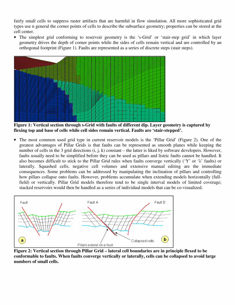
fairly small cells to suppress raster artifactstypes use n general the corner points of cells cell center. • The simplest grid conforming to reservoir geometr

geometry drives the depth of corner points while the sides of cells remain vertical and are controlled by an orthogonal footprint (Figure 1). Faults are represented as a series of discrete steps

Figure 1: Vertical section through s-Grid

flexing top and base of cells while cell sides remain vertical. Faults are ‘stair

• The most common used grid type in current reservoir models greatest advantages of Pillar Grids number of cells in the 3 grid directions (i, j, k) constantfaults usually need to be simplified before they can be used as pillars and listric faults cannot be handled. It also becomes difficult to stick to the Pillar Grid rules laterally. Squashed cells, negative cell volumes and extensive manual editing are the immediate consequences. Some problems can be addressed how pillars collapse onto faults. However, field) or vertically. Pillar Grid models therefore tend to be single interval models of limited coverage; stacked reservoirs would then be handled as a series of individual models that can be co

Figure 2: Vertical section through Pillar Grid

conformable to faults. When faults converge vertically or laterally, cells can be collapsed to avoid large

numbers of small cells.

r artifacts that are harmful in flow simulation. All more sophisticated grid of cells to describe the subsurface geometry; properties can be stored

The simplest grid conforming to reservoir geometry is the ‘s-Grid’ or ‘stair-step grid’ in which layer geometry drives the depth of corner points while the sides of cells remain vertical and are controlled by an

Faults are represented as a series of discrete steps (stair steps).

Grid with faults of different dip. Layer geometry is captured

flexing top and base of cells while cell sides remain vertical. Faults are ‘stair-stepped’.

in current reservoir models is the ‘Pillar Grid’ is that faults can be represented as smooth planes while keeping the

number of cells in the 3 grid directions (i, j, k) constant – the latter is liked by software developers. However, faults usually need to be simplified before they can be used as pillars and listric faults cannot be handled. It also becomes difficult to stick to the Pillar Grid rules when faults converge vertically (‘Y’ or ‘laterally. Squashed cells, negative cell volumes and extensive manual editing are the immediate

Some problems can be addressed by manipulating the inclination of pillarsowever, problems accumulate when extending models horizontally (full

models therefore tend to be single interval models of limited coverage; then be handled as a series of individual models that can be co

Pillar Grid – lateral cell boundaries are in principle

hen faults converge vertically or laterally, cells can be collapsed to avoid large

. All more sophisticated grid properties can be stored at the

step grid’ in which layer geometry drives the depth of corner points while the sides of cells remain vertical and are controlled by an

(stair steps).

with faults of different dip. Layer geometry is captured by

stepped’.

’ (Figure 2). One of the is that faults can be represented as smooth planes while keeping the

is liked by software developers. However, faults usually need to be simplified before they can be used as pillars and listric faults cannot be handled. It

when faults converge vertically (‘Y’ or ‘λ’ faults) or laterally. Squashed cells, negative cell volumes and extensive manual editing are the immediate

by manipulating the inclination of pillars and controlling oblems accumulate when extending models horizontally (full-

models therefore tend to be single interval models of limited coverage; then be handled as a series of individual models that can be co-visualized.

in principle flexed to be

hen faults converge vertically or laterally, cells can be collapsed to avoid large

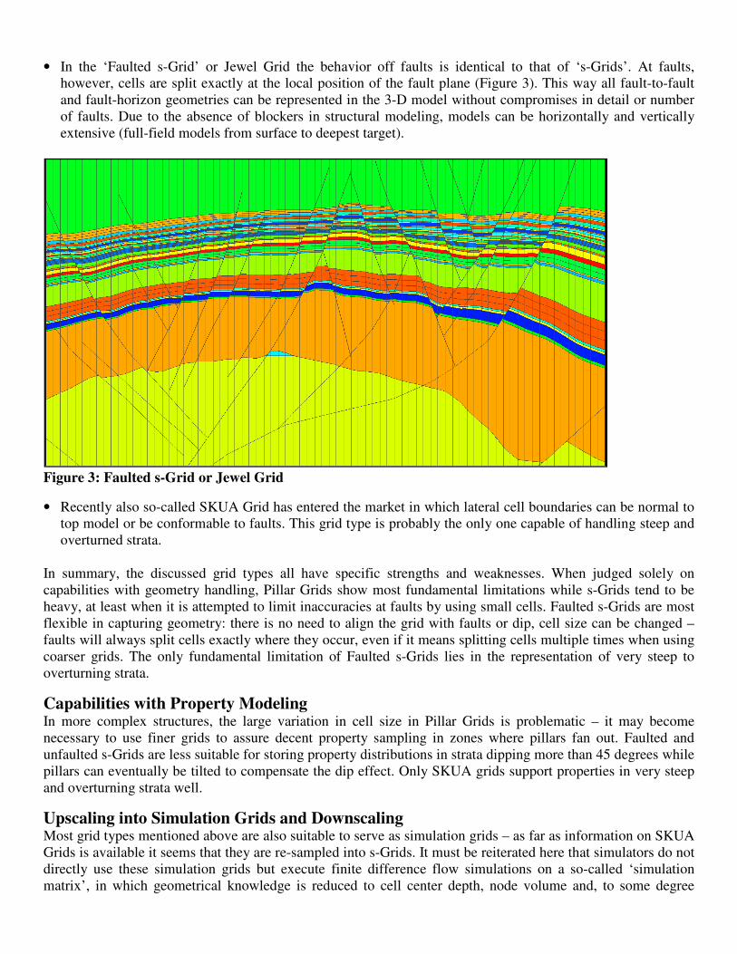
• In the ‘Faulted s-Grid’ or Jewel Grid the behavior off faults is identical to that of ‘s-Grids’. At faults, however, cells are split exactly at the local position of the fault plane (Figure 3). This way all fault-to-fault and fault-horizon geometries can be represented in the 3-D model without compromises in detail or number of faults. Due to the absence of blockers in structural modeling, models can be horizontally and vertically extensive (full-field models from surface to deepest target).

Figure 3: Faulted s-Grid or Jewel Grid

• Recently also so-called SKUA Grid has entered the market in which lateral cell boundaries can be normal to top model or be conformable to faults. This grid type is probably the only one capable of handling steep and overturned strata.

In summary, the discussed grid types all have specific strengths and weaknesses. When judged solely on capabilities with geometry handling, Pillar Grids show most fundamental limitations while s-Grids tend to be heavy, at least when it is attempted to limit inaccuracies at faults by using small cells. Faulted s-Grids are most flexible in capturing geometry: there is no need to align the grid with faults or dip, cell size can be changed – faults will always split cells exactly where they occur, even if it means splitting cells multiple times when using coarser grids. The only fundamental limitation of Faulted s-Grids lies in the representation of very steep to overturning strata.

Capabilities with Property Modeling In more complex structures, the large variation in cell size in Pillar Grids is problematic – it may become necessary to use finer grids to assure decent property sampling in zones where pillars fan out. Faulted and unfaulted s-Grids are less suitable for storing property distributions in strata dipping more than 45 degrees while pillars can eventually be tilted to compensate the dip effect. Only SKUA grids support properties in very steep and overturning strata well.

Upscaling into Simulation Grids and Downscaling Most grid types mentioned above are also suitable to serve as simulation grids – as far as information on SKUA Grids is available it seems that they are re-sampled into s-Grids. It must be reiterated here that simulators do not directly use these simulation grids but execute finite difference flow simulations on a so-called ‘simulation matrix’, in which geometrical knowledge is reduced to cell center depth, node volume and, to some degree

transmissibility's as calculated from permeability and cell contact areatransmissibility's works best if modeling grid and simulation matrix are similar and communicate with each other in terms of integers (e.g. 3 cells in the geological grid to 1 cell in simulation grid and matrix), which is the case for all grid types except for SKUA Grids.reservoir models, in order to “close the loop” between geological modeling and reservoir simulation.

Performance of Grid Types in SimulationThrough the integration of (3rd party) reservoir simulatorscommunicate complex structure and grid properties This process allows for properly handling the polyhedral cells at the fault locations by computing the cell pore volumes and generating the non-neighbor connections across the fault surfaces. An imethod is consistent X and Y permeability values, resulting in more precise transmissibility calculations and reservoir simulation results. A great number of tests have been executed that distributions that are stored in different grid types. Tspeed and gave identical results to s-Grid(unfaulted) SPE1 and SPE10 models. challenging model where the effects of extensively. The two most common dynamic sGrids were evaluated for flow across a model with two producing wells on the other side of permeability's. The fault throw for two faults on the

Figure 4: Kz in the 3 different types of simulation grids of faulted

permeability is displayed on the arbitrary cross

planes are highlighted in green, 2 of which define a fault zone with low

injector is denoted by the blue well with th

The results show that water breakthrough times are different by 50% in Faulted s-Grids (see Figure 5). More importantly, visualization and evaluation of the results would most probably yield significantly different development and in

as calculated from permeability and cell contact area. Upscaling and derivation of works best if modeling grid and simulation matrix are similar and communicate with each

rms of integers (e.g. 3 cells in the geological grid to 1 cell in simulation grid and matrix), which is the case for all grid types except for SKUA Grids. The same holds for downscaling simulation results back into

loop” between geological modeling and reservoir simulation.

Performance of Grid Types in Simulation party) reservoir simulators such as provided by CMG

rid properties directly to the to the reservoir simulation deck generator. This process allows for properly handling the polyhedral cells at the fault locations by computing the cell pore

neighbor connections across the fault surfaces. An important advantage of this method is consistent X and Y permeability values, resulting in more precise transmissibility calculations and

of tests have been executed that compare simulation results in identicalare stored in different grid types. The Faulted s-Grids perform in simulation

Grids when benchmarked in CMG's IMEX simulation engine A more interesting benchmark was conducted on a structurally

model where the effects of grid sampling on transmissibility across faults could be evaluated more The two most common dynamic simulation grids (s-Grid, Pillar Grid) along with the

model using one water injector in dead oil and keeping the BHP constant with two producing wells on the other side of the faults. The model comprises of 10 intervals with altepermeability's. The fault throw for two faults on the left is 540 feet, while single fault on the right is 150 ft.

Kz in the 3 different types of simulation grids of faulted heterogeneous field; vertical

rbitrary cross-section (blue layers ~ 1 Darcy, red layers ~

, 2 of which define a fault zone with low permeability's

injector is denoted by the blue well with the producers shown by the yellow derrick.

The results show that water breakthrough times are different by 50% in Pillar Grids versus the Stair Step and ). More importantly, visualization and evaluation of the results would most

probably yield significantly different development and in-fill drilling planning (see Figure

Upscaling and derivation of works best if modeling grid and simulation matrix are similar and communicate with each

rms of integers (e.g. 3 cells in the geological grid to 1 cell in simulation grid and matrix), which is the The same holds for downscaling simulation results back into

loop” between geological modeling and reservoir simulation.

CMG, Faulted s-Grids can the to the reservoir simulation deck generator.

This process allows for properly handling the polyhedral cells at the fault locations by computing the cell pore mportant advantage of this

method is consistent X and Y permeability values, resulting in more precise transmissibility calculations and

identical structure and property in simulation with equivalent

CMG's IMEX simulation engine on the A more interesting benchmark was conducted on a structurally more

transmissibility across faults could be evaluated more ) along with the Faulted s-

using one water injector in dead oil and keeping the BHP constant intervals with alternating

left is 540 feet, while single fault on the right is 150 ft.

heterogeneous field; vertical

Darcy, red layers ~ 1 mD). 3 fault

permeability's inside. Water

e producers shown by the yellow derrick.

s versus the Stair Step and ). More importantly, visualization and evaluation of the results would most

Figure 6).

Figure 5: IMEX Simulation results showing water breakthrough

model. Arrival time of water front differs by approximately 50%.

Figure 6: Water Saturations after 7609

and near faults being handled differently

In general it can be stated that simulation tests show results from sGiven that s-Grids are most similar in geometry to simulation matrices results from sbe correct if they are fine enough to represent geology properly.understand the differences in simulation behavior.

Grid Types and Integrated WorkflowsIn integrated workflows, the overall performance of the Grid reservoir simulation is by far more critical rather than its performance in individual dito utilize, analyze and interpret all of the subsurface data available in hydrocarbon assets can be greatly facilitated by newer gridding technologies and approaches that can properly deal with the range of scales associated with all data contributing to reservoir performance. Older gridding techniques were devised and implemented in computing environments that were limited in processing and visualization power. Newer application engineering techniques in conjunction with 32 and gridding capabilities that can more effectively manage the scaling challenges associated Integrated Modeling (IRM). Through the realization of the benefits of IRefficiently and effectively managed in a proactive manner saving both time and cost.

IMEX Simulation results showing water breakthrough at Well 3 prediction across faulted

model. Arrival time of water front differs by approximately 50%.

7609 days differ substantially in Pillar Grid due to

and near faults being handled differently.

In general it can be stated that simulation tests show results from s-Grids and Faulted sGrids are most similar in geometry to simulation matrices results from s-Grids can be assumed to

be correct if they are fine enough to represent geology properly. Additional testing is currently ongoing to better ulation behavior.

Grid Types and Integrated Workflows In integrated workflows, the overall performance of the Grid in iterative loops between geological modeling and

is by far more critical rather than its performance in individual discipline areas. to utilize, analyze and interpret all of the subsurface data available in hydrocarbon assets can be greatly facilitated by newer gridding technologies and approaches that can properly deal with the range of scales

h all data contributing to reservoir performance. Older gridding techniques were devised and implemented in computing environments that were limited in processing and visualization power. Newer application engineering techniques in conjunction with 32 and 64 bit desktop operating systems enable new gridding capabilities that can more effectively manage the scaling challenges associated Integrated

). Through the realization of the benefits of IRM, hydrocarbon assets can now be more iciently and effectively managed in a proactive manner saving both time and cost.

prediction across faulted

due to transmissibility's at

Grids and Faulted s-Grids to be similar. Grids can be assumed to

Additional testing is currently ongoing to better

in iterative loops between geological modeling and scipline areas. The ability

to utilize, analyze and interpret all of the subsurface data available in hydrocarbon assets can be greatly facilitated by newer gridding technologies and approaches that can properly deal with the range of scales

h all data contributing to reservoir performance. Older gridding techniques were devised and implemented in computing environments that were limited in processing and visualization power. Newer

64 bit desktop operating systems enable new gridding capabilities that can more effectively manage the scaling challenges associated Integrated reservoir

, hydrocarbon assets can now be more