Embed Size (px)
Citation preview
SFU, CMPT 459 / 741, 06-3, Martin Ester 64
3. Cluster and Outlier Analysis
Contents of this Chapter
3.1 Introduction
3.2 Partitioning Methods
3.3 Hierarchical Methods
3.4 Density-Based Methods
3.5 Database Techniques for Scalable Clustering
3.6 Clustering High-Dimensional Data
3.7 Outlier Detection
Reference: [Han and Kamber 2006, Chapter 7]
SFU, CMPT 459 / 741, 06-3, Martin Ester 65
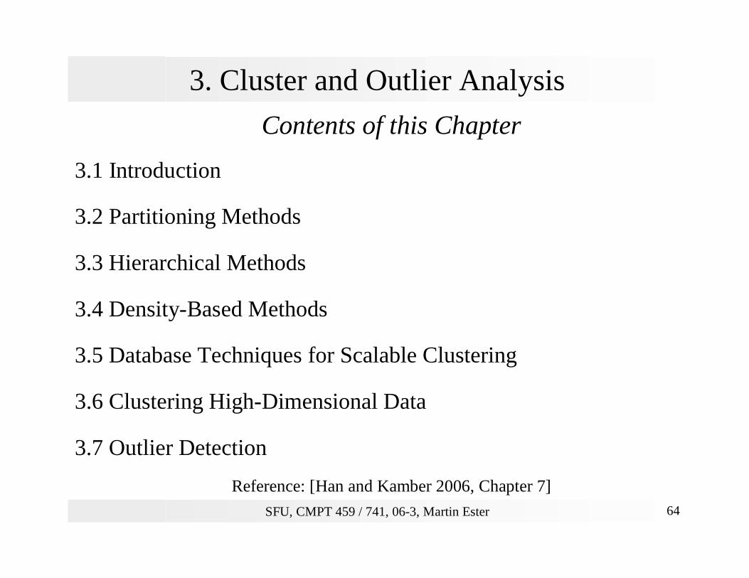
3.1 Introduction
Goal of Cluster Analysis• Identification of a finite set of categories, classes or groups (clusters) in the
dataset• Objects within the same cluster shall be as similar as possible• Objects of different clusters shall be as dissimilar as possible
clusters of different sizes, shapes, densitieshierarchical clustersdisjoint / overlapping clusters
SFU, CMPT 459 / 741, 06-3, Martin Ester 66
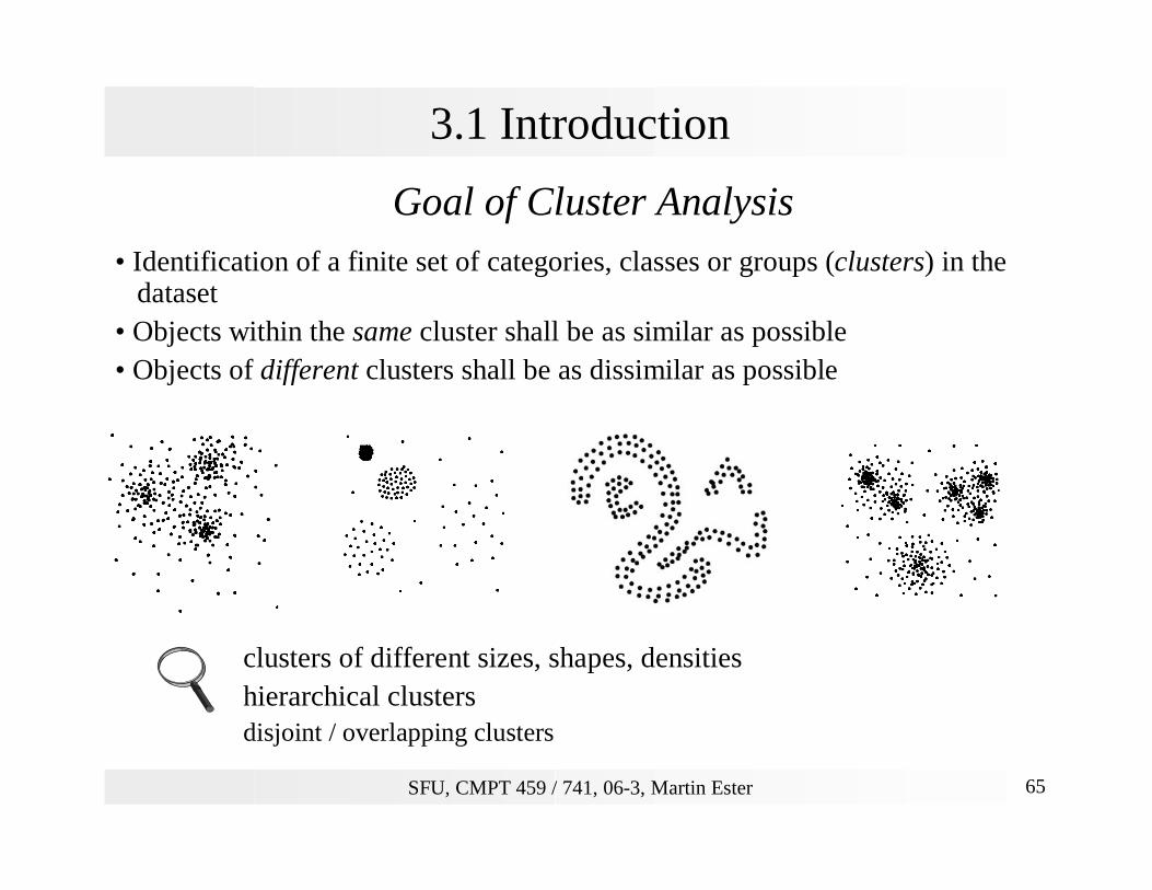
3.1 Introduction
Goal of Outlier Analysis
• Identification of objects (outliers) in the dataset which aresignificantly different from the rest of the dataset (global outliers)or significantly different from their neighbors in the dataset (local outliers)
outliers do not belong to any of the clusters
..
global outliers
local outlier

SFU, CMPT 459 / 741, 06-3, Martin Ester 67
3.1 Introduction
Clustering as Optimization Problem
Definition• dataset D, |D| = n• clustering C of D:
Goalfind clustering that best fits the given training data
Search Spacespace of all clusteringssize is
local optimization methods (greedy)
DCDC
CCC
kiiii
k
=⊆
=
≤≤U1,
1
andwhere
},...,{
)2( nO
SFU, CMPT 459 / 741, 06-3, Martin Ester 68
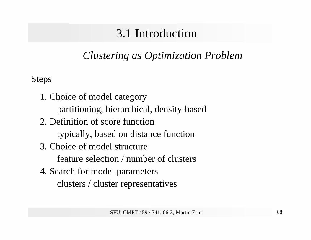
3.1 Introduction
Clustering as Optimization Problem
Steps
1. Choice of model categorypartitioning, hierarchical, density-based
2. Definition of score functiontypically, based on distance function
3. Choice of model structurefeature selection / number of clusters
4. Search for model parameters clusters / cluster representatives
SFU, CMPT 459 / 741, 06-3, Martin Ester 69
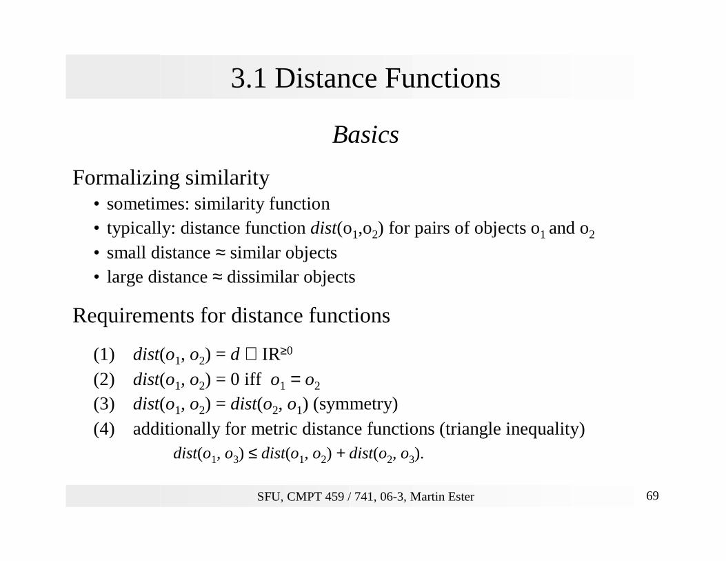
3.1 Distance Functions
Basics
Formalizing similarity• sometimes: similarity function• typically: distance function dist(o1,o2) for pairs of objects o1 and o2
• small distance ≈ similar objects• large distance ≈ dissimilar objects
Requirements for distance functions
(1) dist(o1, o2) = d ∈ IR≥0
(2) dist(o1, o2) = 0 iff o1 = o2
(3) dist(o1, o2) = dist(o2, o1) (symmetry)(4) additionally for metric distance functions (triangle inequality)
dist(o1, o3) ≤ dist(o1, o2) + dist(o2, o3).
SFU, CMPT 459 / 741, 06-3, Martin Ester 70
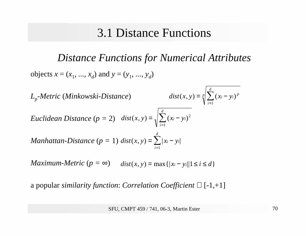
3.1 Distance Functions
Distance Functions for Numerical Attributes
objects x = (x1, ..., xd) and y = (y1, ..., yd)
Lp-Metric (Minkowski-Distance)
Euclidean Distance (p = 2)
Manhattan-Distance (p = 1)
Maximum-Metric (p = ∞)
a popular similarity function: Correlation Coefficient ∈ [-1,+1]
dist x y x yi ip
i
d
p( , ) ( )= −=∑
1
dist x y x yi i
i
d
( , ) ( )= −=∑ 2
1
dist x y x yi i
i
d
( , ) | |= −=∑
1
dist x y x y i di i( , ) max{| || }= − ≤ ≤1
SFU, CMPT 459 / 741, 06-3, Martin Ester 71
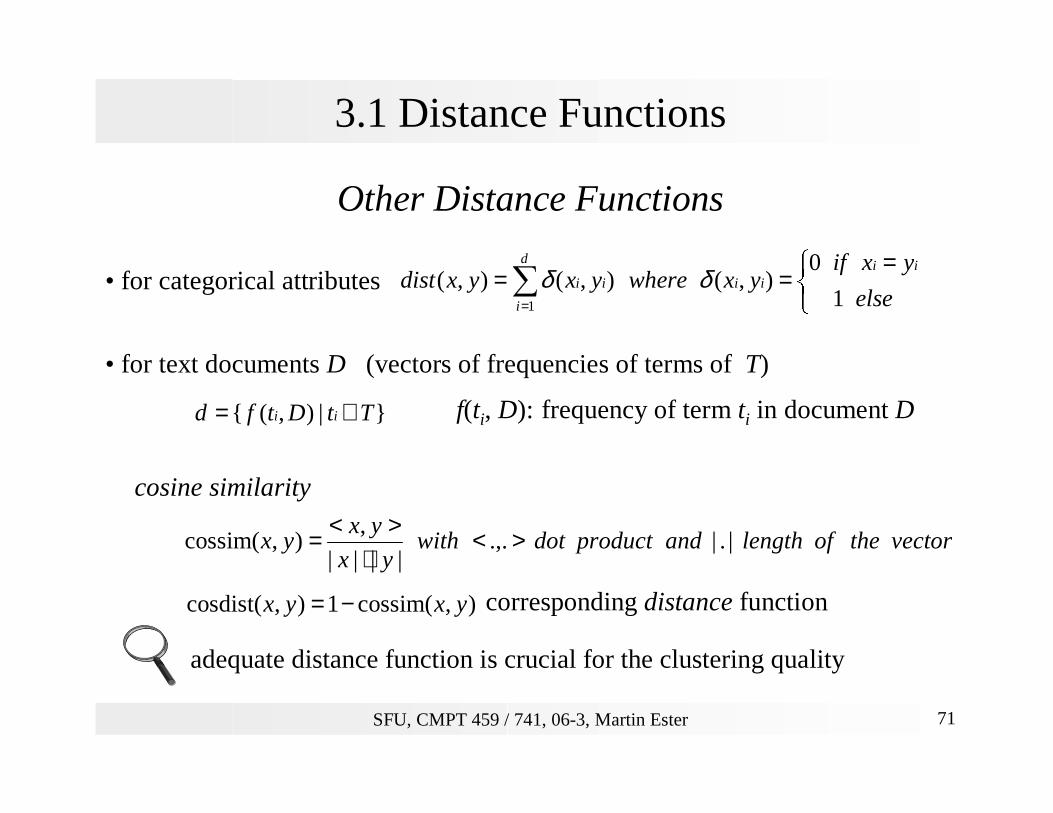
3.1 Distance Functions
Other Distance Functions
• for categorical attributes
• for text documents D (vectors of frequencies of terms of T)
f(ti, D): frequency of term ti in document D
cosine similarity
corresponding distance function
adequate distance function is crucial for the clustering quality
∑=
=
==d
i
iiiiii
else
yxifyxwhereyxyxdist
1 1
0),(),(),( δδ
}|),({ TtDtfd ii ∈=
vectortheoflengthandproductdotwithyx
yxyx |.|.,.
||||
,),cossim( ><
⋅><=
),cossim(1),cosdist( yxyx −=
SFU, CMPT 459 / 741, 06-3, Martin Ester 72
3.1 Typical Clustering Applications
Overview
• Market segmentation
clustering the set of customer transactions
• Determining user groups on the WWW
clustering web-logs
• Structuring large sets of text documents
hierarchical clustering of the text documents
• Generating thematic maps from satellite images
clustering sets of raster images of the same area (feature vectors)
SFU, CMPT 459 / 741, 06-3, Martin Ester 73
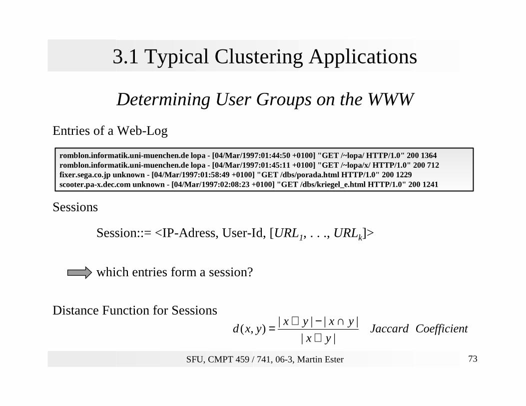
3.1 Typical Clustering Applications
Determining User Groups on the WWW
Entries of a Web-Log
Sessions
Session::= <IP-Adress, User-Id, [URL1, . . ., URLk]>
which entries form a session?
Distance Function for Sessions
romblon.informatik.uni-muenchen.de lopa - [04/Mar/1997:01:44:50 +0100] "GET /~lopa/ HTTP/1.0" 200 1364romblon.informatik.uni-muenchen.de lopa - [04/Mar/1997:01:45:11 +0100] "GET /~lopa/x/ HTTP/1.0" 200 712fixer.sega.co.jp unknown - [04/Mar/1997:01:58:49 +0100] "GET /dbs/porada.html HTTP/1.0" 200 1229scooter.pa-x.dec.com unknown - [04/Mar/1997:02:08:23 +0100] "GET /dbs/kriegel_e.html HTTP/1.0" 200 1241
tCoefficienJaccardyx
yxyxyxd
||
||||),(
∪∩−∪=
SFU, CMPT 459 / 741, 06-3, Martin Ester 74
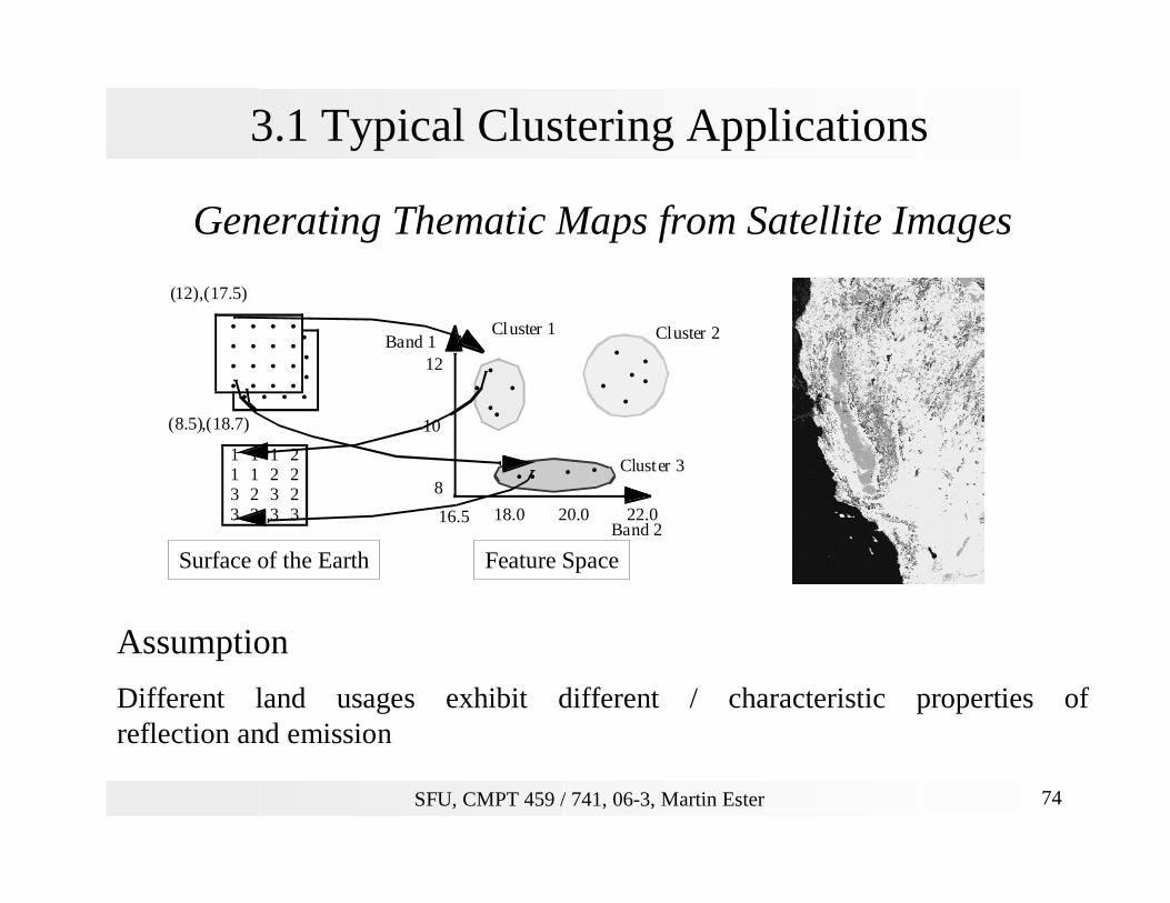
3.1 Typical Clustering Applications
Generating Thematic Maps from Satellite Images
Assumption
Different land usages exhibit different / characteristic properties of reflection and emission
• • • •• • • •• • • •• • • •
• • • •• • • •• • • •• • • •
Erdoberfläche Feature-Raum
Band 1
Band 216.5 22.020.018.0
8
12
10
•
(12),(17.5)
(8.5),(18.7)
•• •
•
••• •
••
••••1 1 1 21 1 2 23 2 3 23 3 3 3
Cluster 1 Cluster 2
Cluster 3
Surface of the Earth Feature Space
SFU, CMPT 459 / 741, 06-3, Martin Ester 75
3.1 Types of Clustering Methods
Partitioning Methods• Parameters: number k of clusters, distance function• determines a „flat“ clustering into k clusters (with minimal costs)
Hierarchical Methods• Parameters: distance function for objects and for clusters• determines a hierarchy of clusterings, merges always the most similar
clusters
Density-Based Methods• Parameters: minimum density within a cluster, distance function• extends cluster by neighboring objects as long as the density is large enough
Other Clustering Methods• Fuzzy Clustering• Graph-based Methods• Neural Networks
SFU, CMPT 459 / 741, 06-3, Martin Ester 76
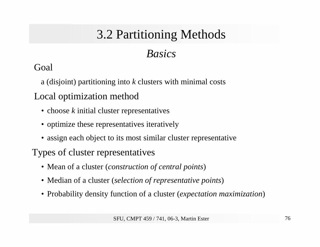
3.2 Partitioning Methods
BasicsGoal
a (disjoint) partitioning into k clusters with minimal costs
Local optimization method
• choose k initial cluster representatives
• optimize these representatives iteratively
• assign each object to its most similar cluster representative
Types of cluster representatives
• Mean of a cluster (construction of central points)
• Median of a cluster (selection of representative points)
• Probability density function of a cluster (expectation maximization)
SFU, CMPT 459 / 741, 06-3, Martin Ester 77
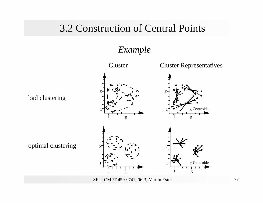
3.2 Construction of Central Points
1
1
5
5
x Centroide
x
xx
1
1
5
5
x Centroidex
x
x
1
1
5
5
1
1
5
5
Example
Cluster Cluster Representatives
bad clustering
optimal clustering
SFU, CMPT 459 / 741, 06-3, Martin Ester 78
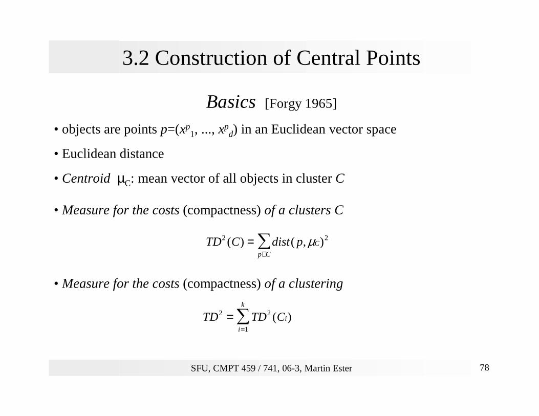
3.2 Construction of Central Points
Basics [Forgy 1965]
• objects are points p=(xp1, ..., xp
d) in an Euclidean vector space
• Euclidean distance
• Centroid µC: mean vector of all objects in cluster C
• Measure for the costs (compactness) of a clusters C
• Measure for the costs (compactness) of a clustering
TD C dist p C
p C
2 2( ) ( , )=∈∑ µ
TD TD Ci
i
k2 2
1
==∑ ( )
SFU, CMPT 459 / 741, 06-3, Martin Ester 79
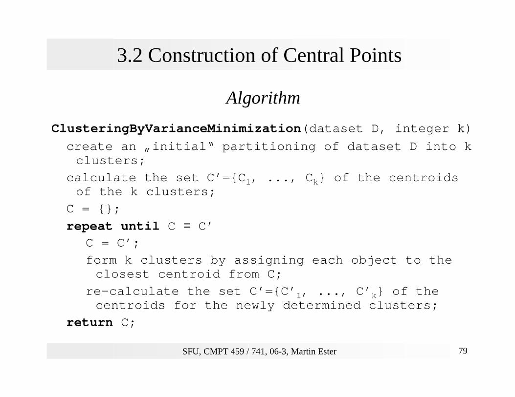
3.2 Construction of Central Points
Algorithm
ClusteringByVarianceMinimization(dataset D, integer k)
create an „initial“ partitioning of dataset D into k clusters;
calculate the set C’={C1, ..., Ck} of the centroidsof the k clusters;
C = {};
repeat until C = C’C = C’;
form k clusters by assigning each object to the closest centroid from C;
re-calculate the set C’={C’1, ..., C’k} of the centroids for the newly determined clusters;
return C;
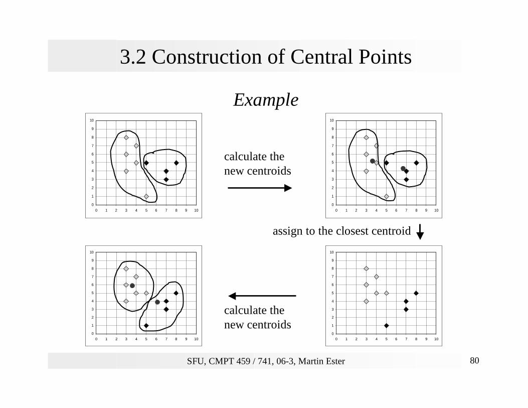
SFU, CMPT 459 / 741, 06-3, Martin Ester 80
3.2 Construction of Central Points
Example
0
1
2
3
4
5
6
7
8
9
10
0 1 2 3 4 5 6 7 8 9 100
1
2
3
4
5
6
7
8
9
10
0 1 2 3 4 5 6 7 8 9 10
0
1
2
3
4
5
6
7
8
9
10
0 1 2 3 4 5 6 7 8 9 10
0
1
2
3
4
5
6
7
8
9
10
0 1 2 3 4 5 6 7 8 9 10
calculate thenew centroids
assign to the closest centroid
calculate thenew centroids
SFU, CMPT 459 / 741, 06-3, Martin Ester 81
3.2 Construction of Central Points
Variants of the Basic Algorithm
k-means [MacQueen 67]
• Idea: the relevant centroids are updated immediately when an object changesits cluster membership
• K-means inherits most properties from the basic algorithm
• K-means depends on the order of objects
ISODATA• based on k-means • post-processing of the resulting clustering by
– elimination of very small clusters– merging and splitting of clusters
• user has to provide several additional parameter values
SFU, CMPT 459 / 741, 06-3, Martin Ester 82
3.2 Construction of Central Points
Discussion
+ EfficiencyRuntime: O(n) for one iteration,
number of iterations is typically small (~ 5 - 10).
+ simple implementation
K-means is the most popular partitioning clustering method
- sensitivity to noise and outliers all objects influence the calculation of the centroid
- all clusters have a convex shape
- the number k of clusters is often hard to determine
- highly dependent from the initial partitioning clustering result as well as runtime
SFU, CMPT 459 / 741, 06-3, Martin Ester 83
3.2 Selection of Representative Points
Basics [Kaufman & Rousseeuw 1990]
• Assumes only a distance function for pairs of objects
• Medoid: a representative element of the cluster (representative point)
• Measure for the costs (compactness) of a clusters C
• Measure for the costs (compactness) of a clustering
• Search space for the clustering algorithm:all subsets of cardinality k of the dataset D with |D|= n
runtime complexity of exhaustive search O(nk)
TD C dist p mC
p C
( ) ( , )=∈∑
TD TD Ci
i
k
==∑ ( )
1
SFU, CMPT 459 / 741, 06-3, Martin Ester 84
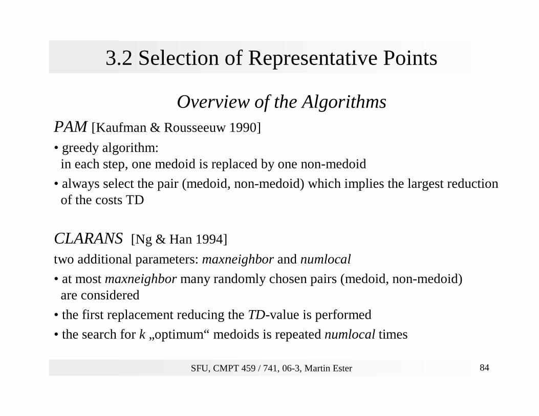
3.2 Selection of Representative Points
Overview of the AlgorithmsPAM [Kaufman & Rousseeuw 1990]
• greedy algorithm:in each step, one medoid is replaced by one non-medoid
• always select the pair (medoid, non-medoid) which implies the largest reductionof the costs TD
CLARANS [Ng & Han 1994]
two additional parameters: maxneighbor and numlocal
• at most maxneighbor many randomly chosen pairs (medoid, non-medoid)are considered
• the first replacement reducing the TD-value is performed
• the search for k „optimum“ medoids is repeated numlocal times
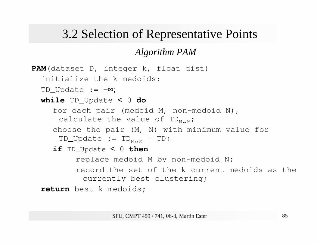
SFU, CMPT 459 / 741, 06-3, Martin Ester 85
3.2 Selection of Representative PointsAlgorithm PAM
PAM(dataset D, integer k, float dist)initialize the k medoids;
TD_Update := −∞;while TD_Update < 0 do
for each pair (medoid M, non-medoid N),calculate the value of TDN↔M;
choose the pair (M, N) with minimum value forTD_Update := TDN↔M − TD;
if TD_Update < 0 thenreplace medoid M by non-medoid N;
record the set of the k current medoids as thecurrently best clustering;
return best k medoids;
SFU, CMPT 459 / 741, 06-3, Martin Ester 86
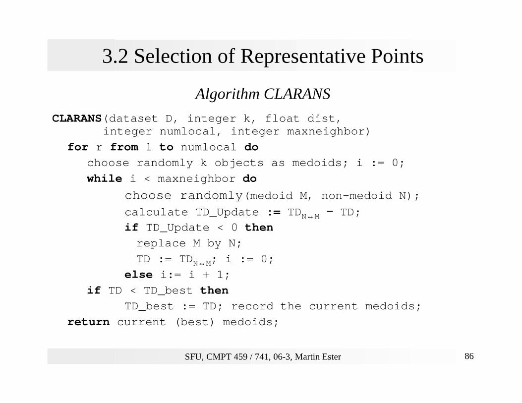
3.2 Selection of Representative Points
Algorithm CLARANS
CLARANS(dataset D, integer k, float dist, integer numlocal, integer maxneighbor)
for r from 1 to numlocal do
choose randomly k objects as medoids; i := 0;
while i < maxneighbor do
choose randomly(medoid M, non-medoid N);calculate TD_Update := TDN↔M − TD;if TD_Update < 0 then
replace M by N;
TD := TDN↔M; i := 0;
else i:= i + 1;
if TD < TD_best then
TD_best := TD; record the current medoids;
return current (best) medoids;
SFU, CMPT 459 / 741, 06-3, Martin Ester 87
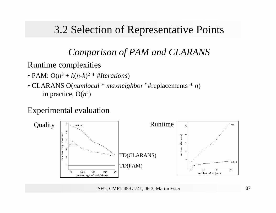
3.2 Selection of Representative Points
Comparison of PAM and CLARANSRuntime complexities• PAM: O(n3 + k(n-k)2 * #Iterations)
• CLARANS O(numlocal * maxneighbor * #replacements * n)in practice, O(n2)
Experimental evaluation
TD(CLARANS)
TD(PAM)
Quality Runtime
SFU, CMPT 459 / 741, 06-3, Martin Ester 88
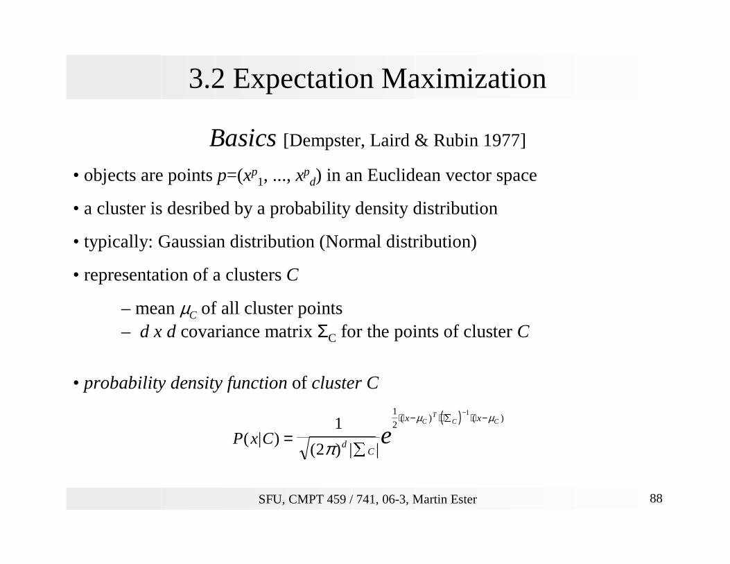
3.2 Expectation Maximization
Basics [Dempster, Laird & Rubin 1977]
• objects are points p=(xp1, ..., xp
d) in an Euclidean vector space
• a cluster is desribed by a probability density distribution
• typically: Gaussian distribution (Normal distribution)
• representation of a clusters C
– mean µC of all cluster points– d x d covariance matrix ΣC for the points of cluster C
• probability density function of cluster C
( )P x C
x x
dC
CT
C C
e( | )( ) | |
( ) ( )
=∑
⋅ − ⋅ ∑ ⋅ −−1
21
1
2
µ µ
π
SFU, CMPT 459 / 741, 06-3, Martin Ester 89
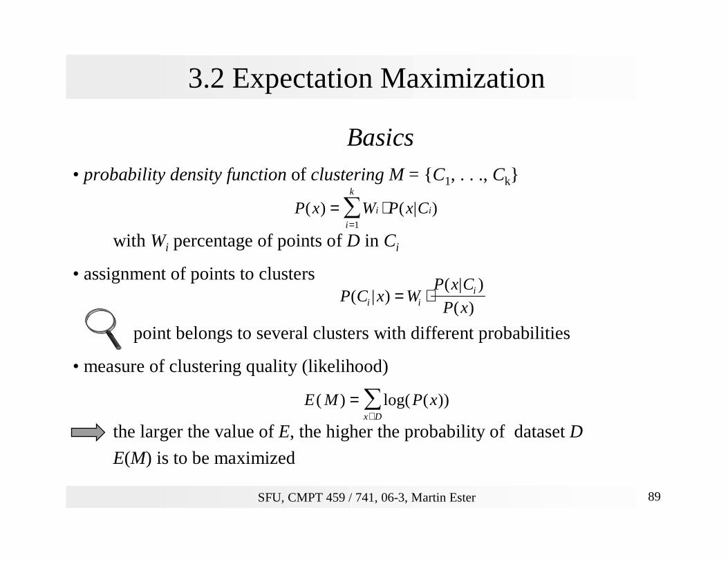
3.2 Expectation Maximization
Basics• probability density function of clustering M = {C1, . . ., Ck}
with Wi percentage of points of D in Ci
• assignment of points to clusters
point belongs to several clusters with different probabilities
• measure of clustering quality (likelihood)
the larger the value of E, the higher the probability of dataset D
E(M) is to be maximized
P x W P x Ci i
i
k
( ) ( | )= ⋅=∑
1
P C x WP x C
P xi ii( | )
( | )
( )= ⋅
E M P xx D
( ) log( ( ))=∈∑
SFU, CMPT 459 / 741, 06-3, Martin Ester 90
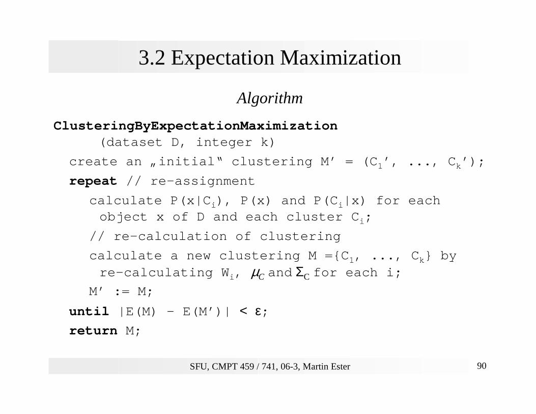
3.2 Expectation Maximization
Algorithm
ClusteringByExpectationMaximization (dataset D, integer k)
create an „initial“ clustering M’ = (C1’, ..., Ck’);
repeat // re-assignment
calculate P(x|Ci), P(x) and P(Ci|x) for each object x of D and each cluster Ci;
// re-calculation of clustering
calculate a new clustering M ={C1, ..., Ck} byre-calculating Wi, µC and ΣC for each i;
M’ := M;
until |E(M) - E(M’)| < ε;return M;
SFU, CMPT 459 / 741, 06-3, Martin Ester 91
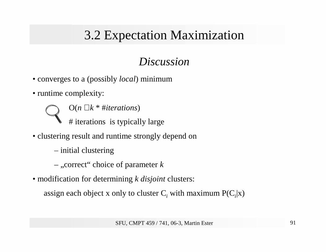
3.2 Expectation Maximization
Discussion
• converges to a (possibly local) minimum
• runtime complexity:
O(n ∗ k * #iterations)
# iterations is typically large
• clustering result and runtime strongly depend on
– initial clustering
– „correct“ choice of parameter k
• modification for determining k disjoint clusters:
assign each object x only to cluster Ci with maximum P(Ci|x)
SFU, CMPT 459 / 741, 06-3, Martin Ester 92
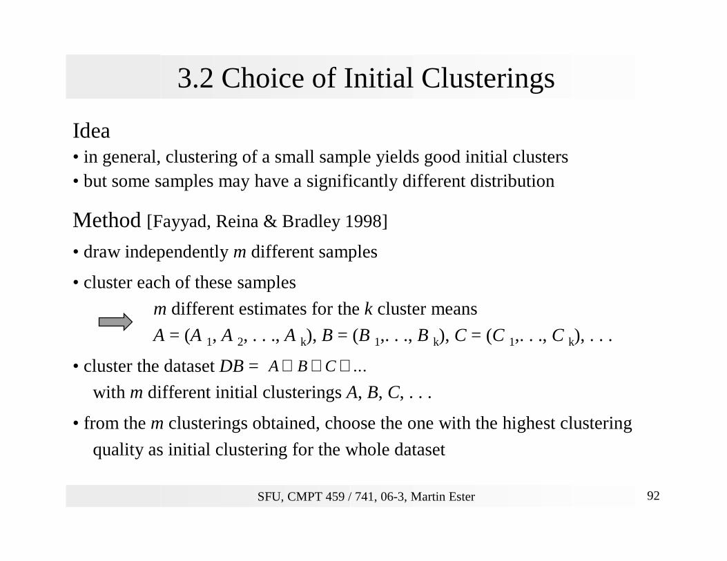
3.2 Choice of Initial Clusterings
Idea• in general, clustering of a small sample yields good initial clusters• but some samples may have a significantly different distribution
Method [Fayyad, Reina & Bradley 1998]
• draw independently m different samples
• cluster each of these samples
m different estimates for the k cluster means
A = (A 1, A 2, . . ., A k), B = (B 1,. . ., B k), C = (C 1,. . ., C k), . . .
• cluster the dataset DB =
with m different initial clusterings A, B, C, . . .
• from the m clusterings obtained, choose the one with the highest clustering
quality as initial clustering for the whole dataset
A B C∪ ∪ ∪ ...

SFU, CMPT 459 / 741, 06-3, Martin Ester 93
3.2 Choice of Initial Clusterings
Example
A2
A1
A3
B1
C1B2
B3
C2
C3
D1
D2
D3
whole dataset
k = 3
DB
from m = 4 samples
true cluster means
SFU, CMPT 459 / 741, 06-3, Martin Ester 94
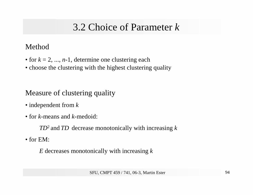
3.2 Choice of Parameter k
Method
• for k = 2, ..., n-1, determine one clustering each• choose the clustering with the highest clustering quality
Measure of clustering quality
• independent from k
• for k-means and k-medoid:
TD2 and TD decrease monotonically with increasing k
• for EM:
E decreases monotonically with increasing k
SFU, CMPT 459 / 741, 06-3, Martin Ester 95
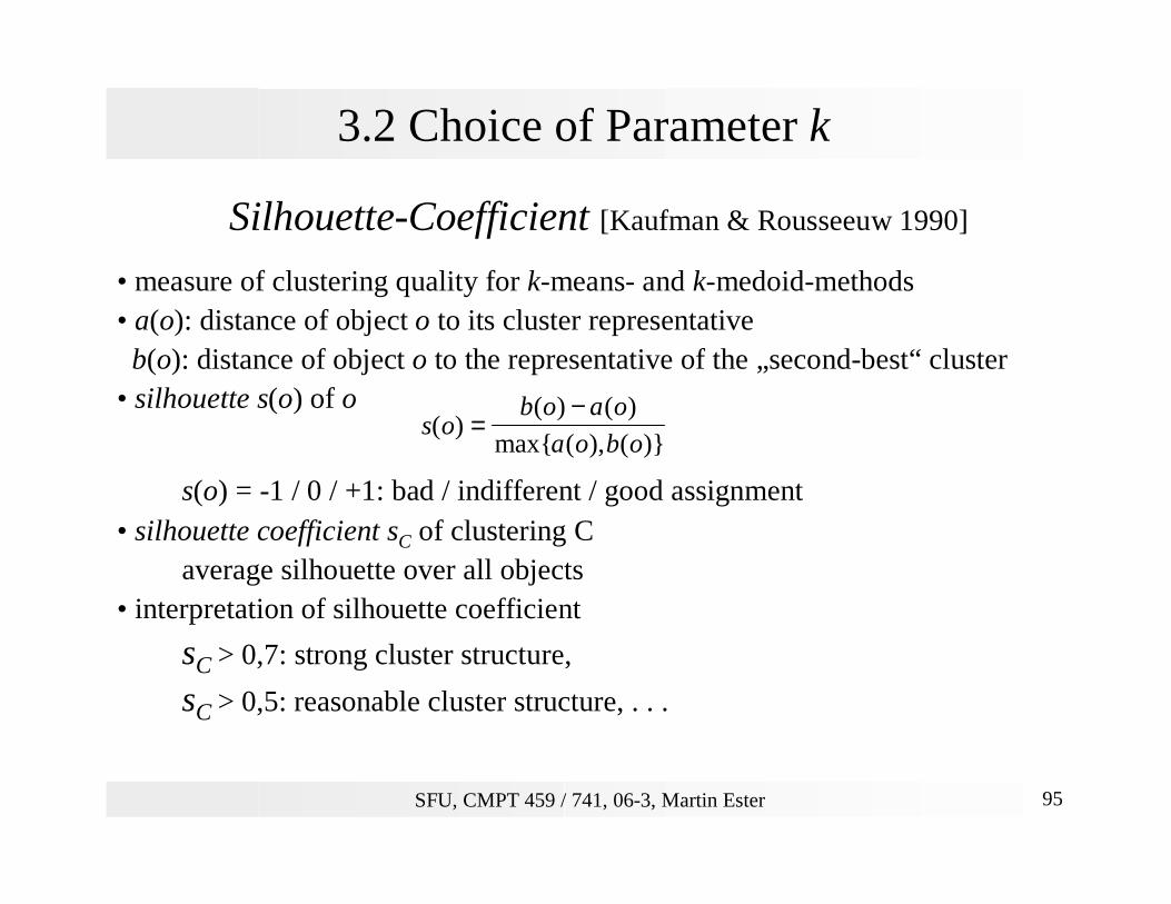
3.2 Choice of Parameter k
Silhouette-Coefficient [Kaufman & Rousseeuw 1990]
• measure of clustering quality for k-means- and k-medoid-methods• a(o): distance of object o to its cluster representative
b(o): distance of object o to the representative of the „second-best“ cluster• silhouette s(o) of o
s(o) = -1 / 0 / +1: bad / indifferent / good assignment• silhouette coefficient sC of clustering C
average silhouette over all objects• interpretation of silhouette coefficient
sC > 0,7: strong cluster structure,
sC > 0,5: reasonable cluster structure, . . .
s ob o a o
a o b o( )
( ) ( )
max{ ( ), ( )}=
−
SFU, CMPT 459 / 741, 06-3, Martin Ester 96
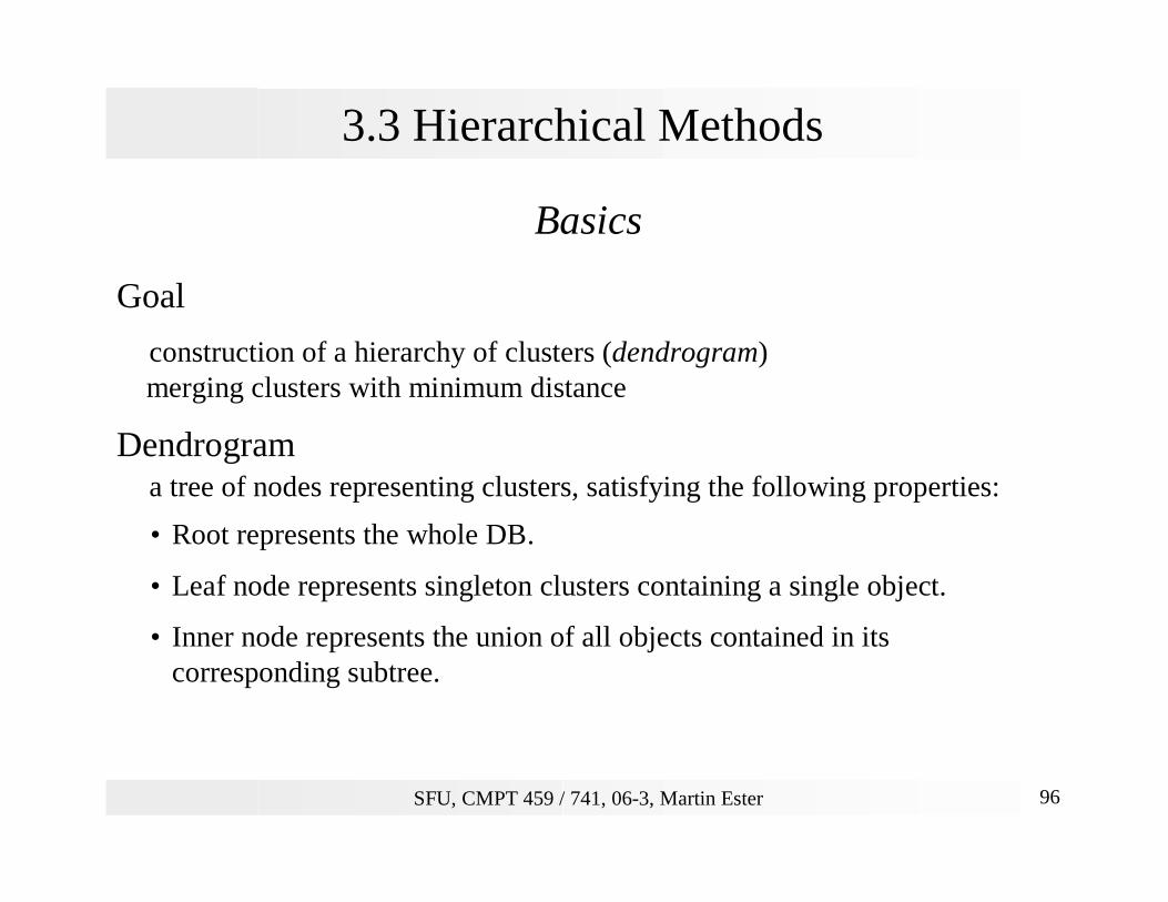
3.3 Hierarchical Methods
Basics
Goal
construction of a hierarchy of clusters (dendrogram) merging clusters with minimum distance
Dendrograma tree of nodes representing clusters, satisfying the following properties:
• Root represents the whole DB.
• Leaf node represents singleton clusters containing a single object.
• Inner node represents the union of all objects contained in its corresponding subtree.
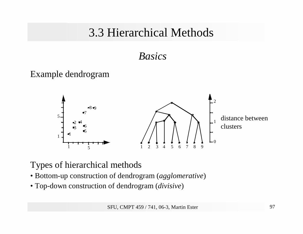
SFU, CMPT 459 / 741, 06-3, Martin Ester 97
3.3 Hierarchical Methods
Basics
Example dendrogram
Types of hierarchical methods• Bottom-up construction of dendrogram (agglomerative)• Top-down construction of dendrogram (divisive)
1
1
5
5
132 4
65
78 9
1 2 3 4 5 6 7 8 90
1
2
distance betweenclusters
SFU, CMPT 459 / 741, 06-3, Martin Ester 98
3.3 Single-Link and Variants
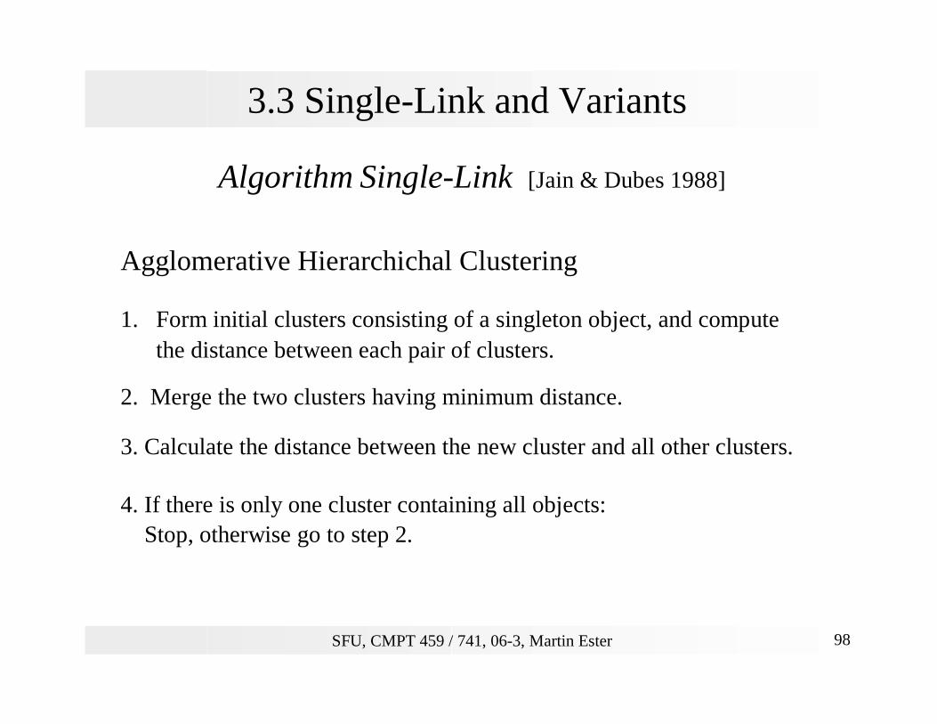
Algorithm Single-Link [Jain & Dubes 1988]
Agglomerative Hierarchichal Clustering
1. Form initial clusters consisting of a singleton object, and computethe distance between each pair of clusters.
2. Merge the two clusters having minimum distance.
3. Calculate the distance between the new cluster and all other clusters.
4. If there is only one cluster containing all objects:Stop, otherwise go to step 2.

SFU, CMPT 459 / 741, 06-3, Martin Ester 99
3.3 Single-Link and Variants
Distance Functions for Clusters
• Let dist(x,y) be a distance function for pairs of objects x, y.
• Let X, Y be clusters, i.e. sets of objects.
Single-Link
Complete-Link
Average-Link
),(min),(_,
yxdistYXsldistYyXx ∈∈
=
),(max),(_,
yxdistYXcldistYyXx ∈∈
=
∑∈∈
⋅⋅
=YyXx
yxdistYX
YXaldist,
),(||||
1),(_
SFU, CMPT 459 / 741, 06-3, Martin Ester 100
3.3 Single-Link and Variants
Discussion
+ does not require knowledge of the number k of clusters
+ finds not only a „flat“ clustering, but a hierarchy of clusters (dendrogram)
+ a single clustering can be obtained from the dendrogram (e.g., by performing a horizontal cut)
- decisions (merges/splits) cannot be undone
- sensitive to noise (Single-Link)a „line“ of objects can connect two clusters
- inefficientruntime complexity at least O(n2) for n objects

SFU, CMPT 459 / 741, 06-3, Martin Ester 101
3.3 Single-Link and Variants
CURE [Guha, Rastogi & Shim 1998]• representation of a cluster
partitioning methods: one objecthierarchical methods: all objects
• CURE: representation of a cluster by c representatives• representatives are stretched by factor of α w.r.t. the centroid
detects non-convex clustersavoids Single-Link effect
SFU, CMPT 459 / 741, 06-3, Martin Ester 102
3.4 Density-Based Clustering
Basics
Idea
• clusters as dense areas in a d-dimensional dataspace
• separated by areas of lower density
Requirements for density-based clusters
• for each cluster object, the local density exceeds some threshold
• the set of objects of one cluster must be spatially connected
Strenghts of density-based clustering
• clusters of arbitrary shape
• robust to noise
• efficiency
SFU, CMPT 459 / 741, 06-3, Martin Ester 103
3.4 Density-Based Clustering
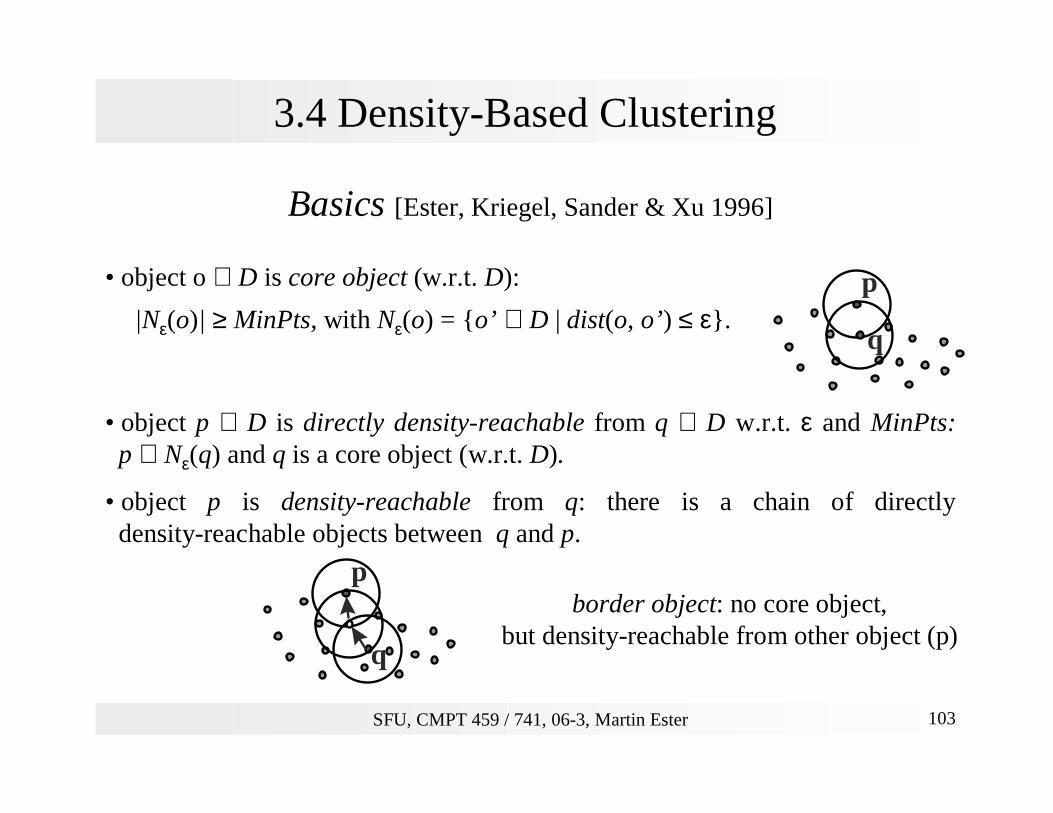
Basics [Ester, Kriegel, Sander & Xu 1996]
• object o ∈ D is core object (w.r.t. D):
|Nε(o)| ≥ MinPts, with Nε(o) = {o’ ∈ D | dist(o, o’) ≤ ε}.
• object p ∈ D is directly density-reachable from q ∈ D w.r.t. ε and MinPts: p ∈ Nε(q) and q is a core object (w.r.t. D).
• object p is density-reachable from q: there is a chain of directly density-reachable objects between q and p.
p
q
p
q
border object: no core object,but density-reachable from other object (p)
SFU, CMPT 459 / 741, 06-3, Martin Ester 104
3.4 Density-Based Clustering
Basics
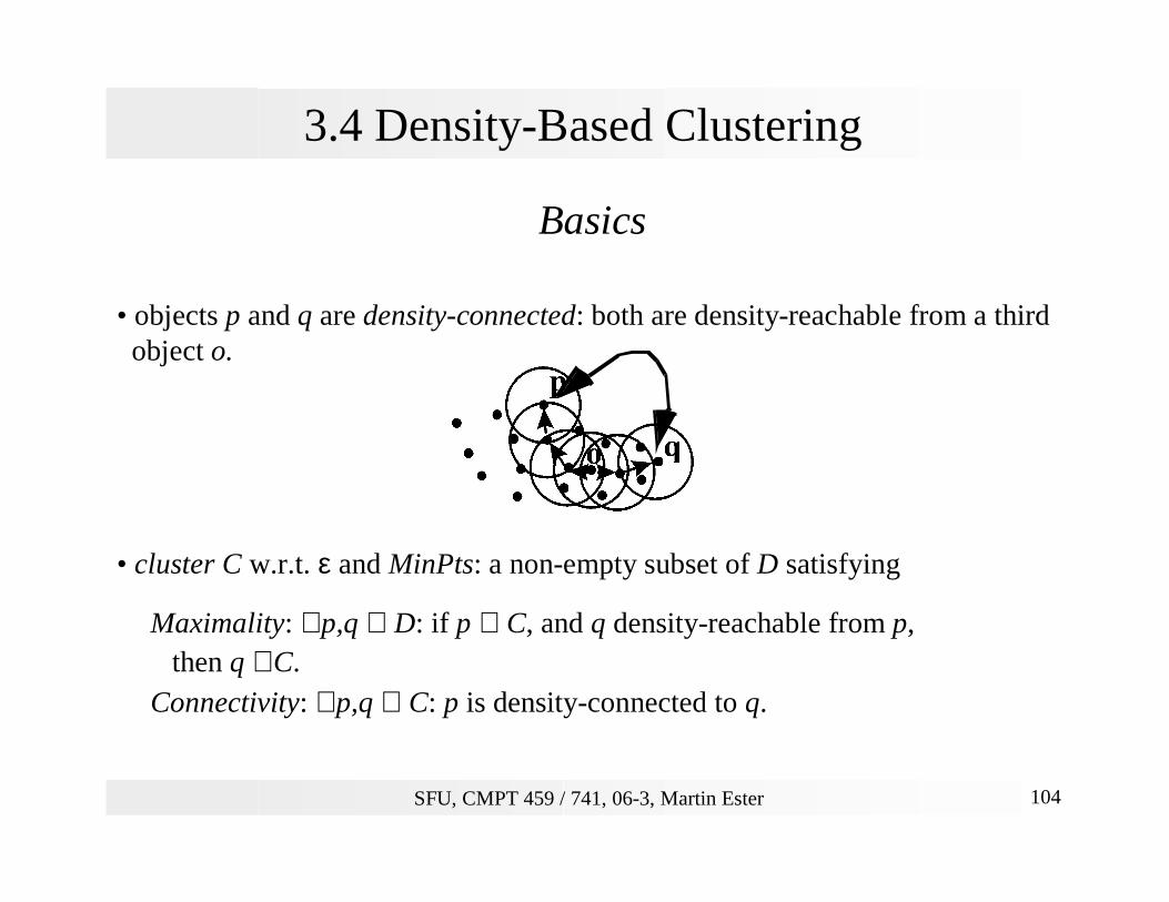
• objects p and q are density-connected: both are density-reachable from a thirdobject o.
• cluster C w.r.t. ε and MinPts: a non-empty subset of D satisfying
Maximality: ∀ p,q ∈ D: if p ∈ C, and q density-reachable from p, then q ∈ C.
Connectivity: ∀ p,q ∈ C: p is density-connected to q.
SFU, CMPT 459 / 741, 06-3, Martin Ester 105
3.4 Density-Based Clustering
Basics
• Clustering
A density-based clustering CL of a dataset D w.r.t. ε and MinPts is the
set of all density-based clusters w.r.t. ε and MinPts in D.
• The set NoiseCL („noise“) is defined as the set of all objects in D which do not
belong to any of the clusters.
• Property
Let C be a density-based cluster and p ∈ C a core object. Then:
C = {o ∈ D | o density-reachable from p w.r.t. ε and MinPts}.
SFU, CMPT 459 / 741, 06-3, Martin Ester 106
3.4 Density-Based Clustering
Algorithm DBSCAN
DBSCAN(dataset D, float ε, integer MinPts)// all objects are initially unclassified,
// o.ClId = UNCLASSIFIED for all o ∈ D
ClusterId := nextId(NOISE);
for i from 1 to |D| do
object := D.get(i);
if Objekt.ClId = UNCLASSIFIED then
if ExpandCluster(D, object, ClusterId, ε, MinPts)// visits all objects in D density-reachable from object
then ClusterId:=nextId(ClusterId);
SFU, CMPT 459 / 741, 06-3, Martin Ester 107
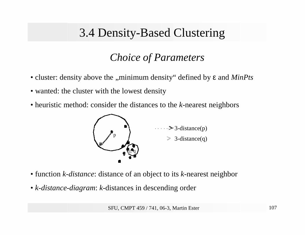
3.4 Density-Based Clustering
Choice of Parameters
• cluster: density above the „minimum density“ defined by ε and MinPts
• wanted: the cluster with the lowest density
• heuristic method: consider the distances to the k-nearest neighbors
• function k-distance: distance of an object to its k-nearest neighbor
• k-distance-diagram: k-distances in descending order
p
q
3-distance(p)
3-distance(q)

SFU, CMPT 459 / 741, 06-3, Martin Ester 108
3.4 Density-Based Clustering
Choice of Parameters
Example
Heuristic Method
• User specifies a value for k (Default is k = 2*d - 1), MinPts := k+1.• System calculates the k-distance-diagram for the dataset and visualizes it.• User chooses a threshold object from the k-distance-diagram,
ε := k-distance(o).
3-di
stan
ce
objects
threshold object o
first „valley“
SFU, CMPT 459 / 741, 06-3, Martin Ester 109
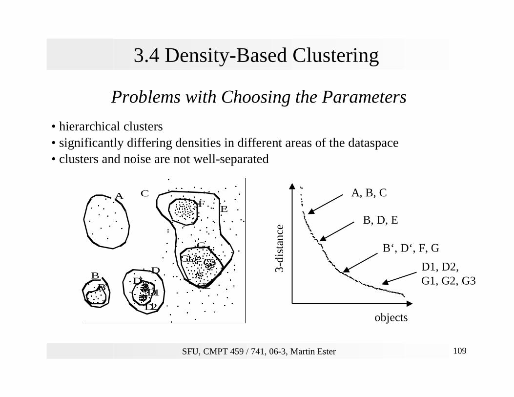
3.4 Density-Based Clustering
Problems with Choosing the Parameters
• hierarchical clusters• significantly differing densities in different areas of the dataspace • clusters and noise are not well-separated
A
B
C
D
E
D’
F
G
B’D1
D2
G1
G2
G3
3-di
stan
ce
objects
A, B, C
B‘, D‘, F, G
B, D, E
D1, D2,G1, G2, G3
SFU, CMPT 459 / 741, 06-3, Martin Ester 110
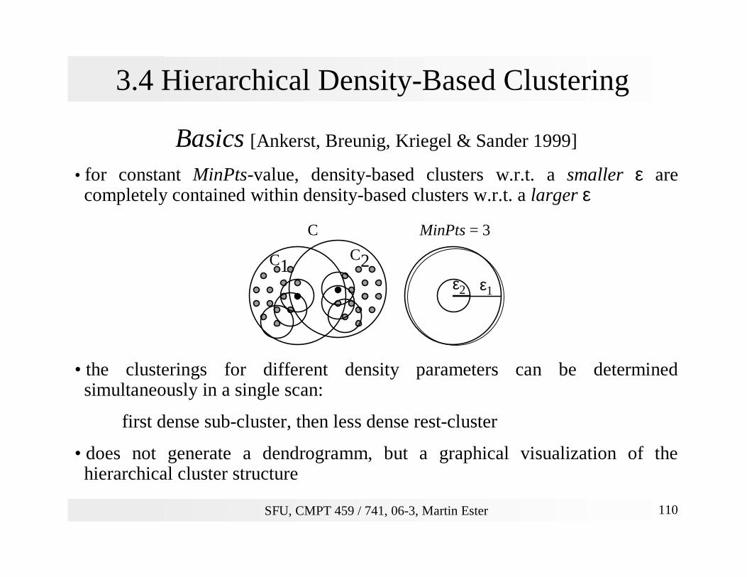
3.4 Hierarchical Density-Based Clustering
Basics [Ankerst, Breunig, Kriegel & Sander 1999]
• for constant MinPts-value, density-based clusters w.r.t. a smaller ε arecompletely contained within density-based clusters w.r.t. a larger ε
• the clusterings for different density parameters can be determinedsimultaneously in a single scan:
first dense sub-cluster, then less dense rest-cluster
• does not generate a dendrogramm, but a graphical visualization of thehierarchical cluster structure
MinPts = 3C
C1C2
ε2 ε1
SFU, CMPT 459 / 741, 06-3, Martin Ester 111
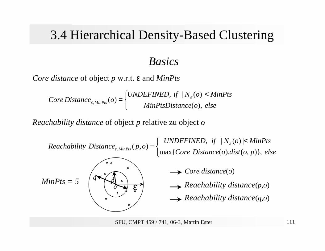
3.4 Hierarchical Density-Based Clustering
BasicsCore distance of object p w.r.t. ε and MinPts
Reachability distance of object p relative zu object o
MinPts = 5
<
=elseoanceMinPtsDist
MinPtsoNifUNDEFINEDoDistanceCore MinPts ,)(
|)(|,)(,
εε
<
=elsepodistoDistanceCore
MinPtsoNifUNDEFINEDopDistancetyReachabili MinPts ,)},(),(max{
|)(|,),(,
εε
opq
ε
Core distance(o)
Reachability distance(p,o)
Reachability distance(q,o)
SFU, CMPT 459 / 741, 06-3, Martin Ester 112
3.4 Hierarchical Density-Based Clustering
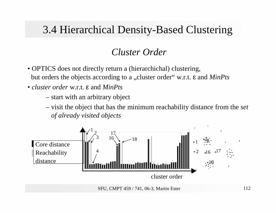
Cluster Order
• OPTICS does not directly return a (hierarchichal) clustering, but orders the objects according to a „cluster order“ w.r.t. ε and MinPts
• cluster order w.r.t. ε and MinPts
– start with an arbitrary object
– visit the object that has the minimum reachability distance from the setof already visited objects
Core-distance
Reachability-distance 4
123 16 18
17
1
2
34
16 17
18
Core distanceReachability distance
cluster order

SFU, CMPT 459 / 741, 06-3, Martin Ester 113
3.4 Hierarchical Density-Based Clustering
Reachability Diagram
• depicts the reachability distances (w.r.t. ε and MinPts) of all objectsin a bar diagram
• with the objects ordered according to the cluster order
reac
habi
lity
dist
ance
reac
habi
lity
dist
ance
clusterorder
SFU, CMPT 459 / 741, 06-3, Martin Ester 114
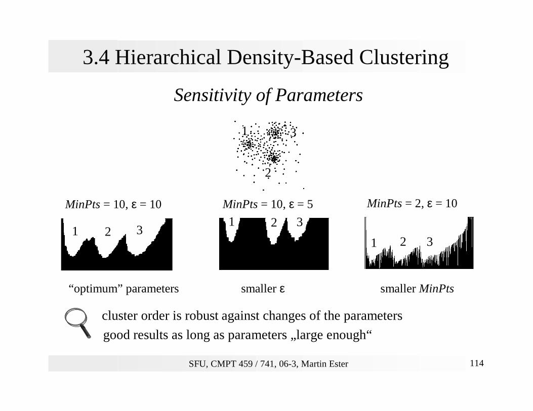
3.4 Hierarchical Density-Based Clustering
Sensitivity of Parameters
1
2
3
MinPts = 10, ε = 10
1 2 3
MinPts = 10, ε = 5 MinPts = 2, ε = 10
1 2 3
1 2 3
“optimum” parameters smaller ε smaller MinPts
cluster order is robust against changes of the parameters
good results as long as parameters „large enough“
SFU, CMPT 459 / 741, 06-3, Martin Ester 115
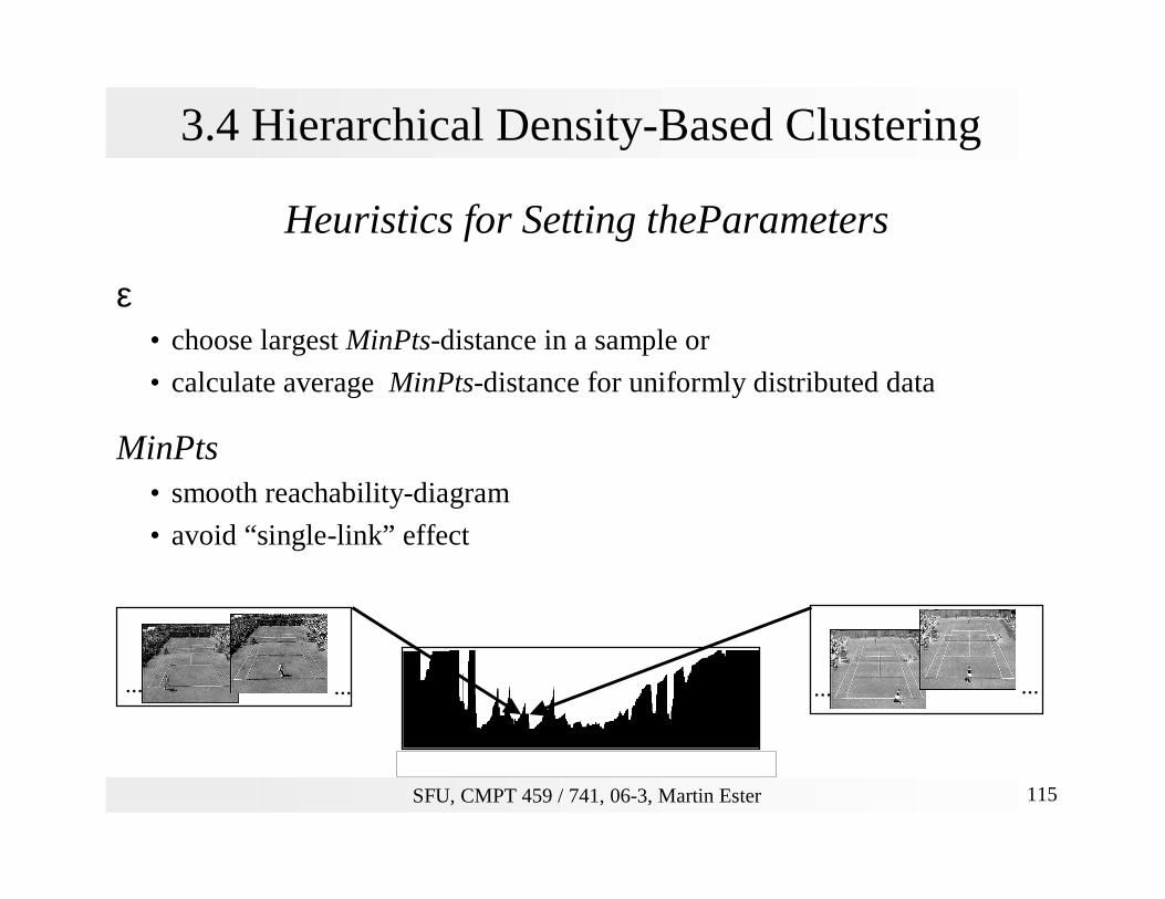
3.4 Hierarchical Density-Based Clustering
Heuristics for Setting theParameters
ε• choose largest MinPts-distance in a sample or
• calculate average MinPts-distance for uniformly distributed data
MinPts• smooth reachability-diagram
• avoid “single-link” effect
... ... ... ...
SFU, CMPT 459 / 741, 06-3, Martin Ester 116
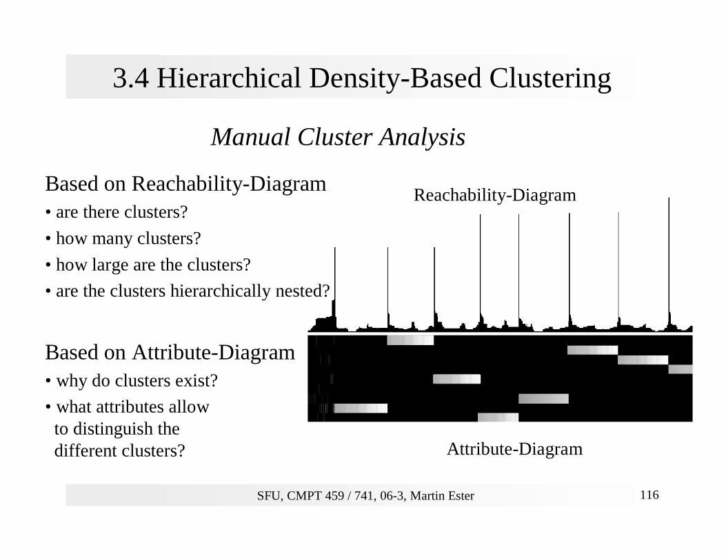
3.4 Hierarchical Density-Based Clustering
Manual Cluster Analysis
Based on Reachability-Diagram• are there clusters?
• how many clusters?
• how large are the clusters?
• are the clusters hierarchically nested?
Based on Attribute-Diagram• why do clusters exist?
• what attributes allowto distinguish the different clusters?
Reachability-Diagram
Attribute-Diagram
SFU, CMPT 459 / 741, 06-3, Martin Ester 117
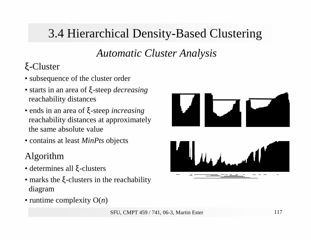
3.4 Hierarchical Density-Based Clustering
Automatic Cluster Analysisξ-Cluster• subsequence of the cluster order
• starts in an area of ξ-steep decreasingreachability distances
• ends in an area of ξ-steep increasingreachability distances at approximatelythe same absolute value
• contains at least MinPts objects
Algorithm• determines all ξ-clusters
• marks the ξ-clusters in the reachabilitydiagram
• runtime complexity O(n)

SFU, CMPT 459 / 741, 06-3, Martin Ester 118
3.5 Database Techniques for Scalable Clustering
Goal
So far
• small datasets• in main memory
Now
• very large datasets which do not fit into main memory• data on secondary storage (pages)
random access orders of magnitude more expensive than in main memory
scalable clustering algorithms
SFU, CMPT 459 / 741, 06-3, Martin Ester 119
3.5 Database Techniques for Scalable Clustering
Use of Spatial Index Structures or Related Techniques
• index structures obtain a coarse pre-clustering (micro-clusters)
neighboring objects are stored on the same / a neighboring disk
block
• index structures are efficient to construct
based on simple heuristics
• fast access methods for similarity queries
e.g. region queries and k-nearest-neighbor queries
SFU, CMPT 459 / 741, 06-3, Martin Ester 120
3.5 Region Queries for Density-Based Clustering
• basic operation for DBSCAN and OPTICS:retrieval of ε-neighborhood for a database object o
• efficient support of such region queries by spatial index structures such as
R-tree, X-tree, M-tree, . . .
• runtime complexities for DBSCAN and OPTICS:
single range query whole algorithm
without index O(n) O(n2)
with index O(log n) O(n log n)
with random access O(1) O(n)
spatial index structures degenerate for very high-dimensional data
SFU, CMPT 459 / 741, 06-3, Martin Ester 121
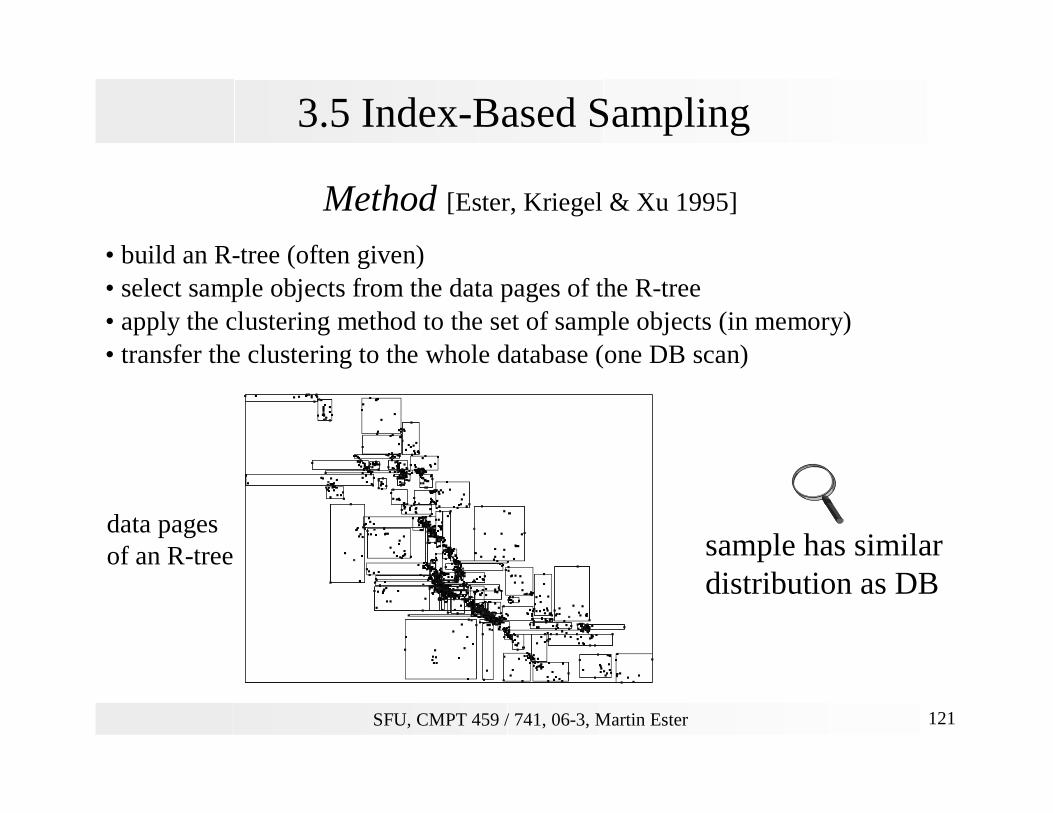
3.5 Index-Based Sampling
Method [Ester, Kriegel & Xu 1995]
• build an R-tree (often given)• select sample objects from the data pages of the R-tree• apply the clustering method to the set of sample objects (in memory)• transfer the clustering to the whole database (one DB scan)
data pagesof an R-tree sample has similar
distribution as DB

SFU, CMPT 459 / 741, 06-3, Martin Ester 122
3.5 Index-Based Sampling
Transfer the Clustering to the whole Database
• For k-means- and k-medoid-methods:
apply the cluster representatives to the whole database (centroids, medoids)
• For density-based methods:generate a representation for each cluster (e.g. bounding box)
assign each object to closest cluster (representation)
• For hierarchichal methods: generation of a hierarchical representation (dendrogram or
reachability-diagram) from the sample is difficult
SFU, CMPT 459 / 741, 06-3, Martin Ester 123
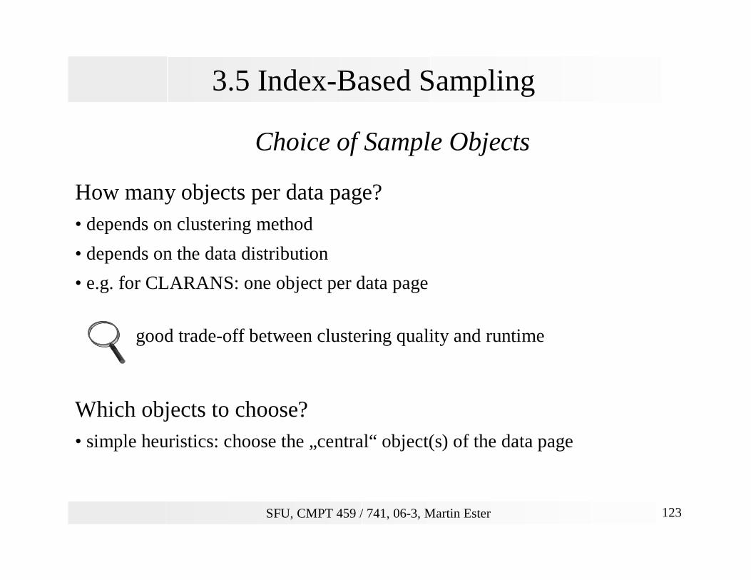
3.5 Index-Based Sampling
Choice of Sample Objects
How many objects per data page?• depends on clustering method
• depends on the data distribution
• e.g. for CLARANS: one object per data page
good trade-off between clustering quality and runtime
Which objects to choose?• simple heuristics: choose the „central“ object(s) of the data page
SFU, CMPT 459 / 741, 06-3, Martin Ester 124
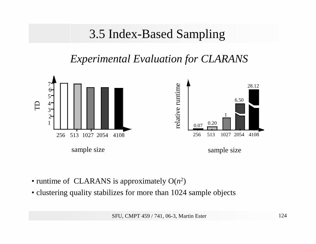
3.5 Index-Based Sampling
Experimental Evaluation for CLARANS
• runtime of CLARANS is approximately O(n2)
• clustering quality stabilizes for more than 1024 sample objects
256 1027
45
2
7
1
3
6
2054 4108513
sample size
TD
256 513 1027
1
6.50
0.07
28.12
2054 4108
0.20
sample size
rela
tive
run
tim
e
SFU, CMPT 459 / 741, 06-3, Martin Ester 125
3.5 Data Compression for Pre-Clustering
Basics [Zhang, Ramakrishnan & Linvy 1996]
Method
• determine compact summaries of “micro-clusters” (Clustering Features)
• hierarchical organization of clustering features
in a balanced tree (CF-tree)
• apply any clustering algorithm, e.g. CLARANS
to the leaf entries (micro-clusters) of the CF-tree
CF-tree
• compact, hierarchichal representation of the database
• conserves the “cluster structure”
SFU, CMPT 459 / 741, 06-3, Martin Ester 126
3.5 Data Compression for Pre-Clustering
Basics
Clustering Feature of a set C of points Xi: CF = (N, LS, SS)
N = |C| number of points in C
linear sum of the N points
square sum of the N points
CFs sufficient to calculate
• centroid
• measures of compactness
• and distance functions for clusters
LS Xii
N
==∑
1
SS Xi
i
N
==∑ 2
1
SFU, CMPT 459 / 741, 06-3, Martin Ester 127
3.5 Data Compression for Pre-Clustering
Basics
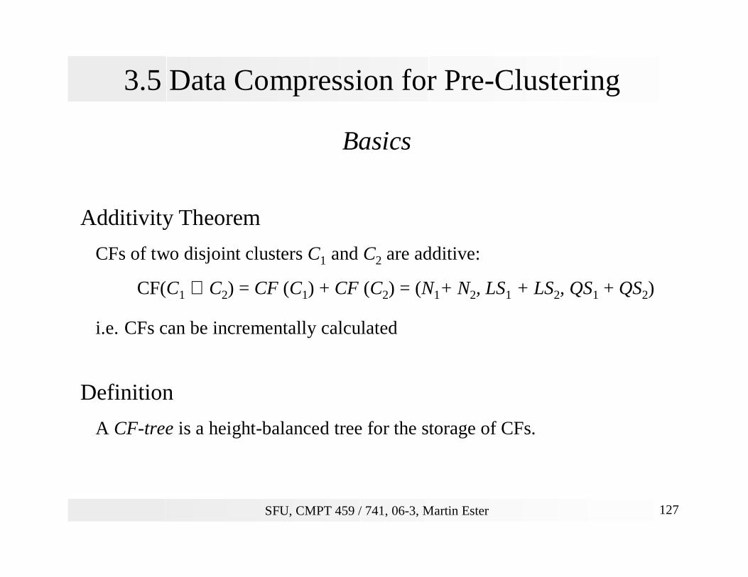
Additivity Theorem
CFs of two disjoint clusters C1 and C2 are additive:
CF(C1 ∪ C2) = CF (C1) + CF (C2) = (N1+ N2, LS1 + LS2, QS1 + QS2)
i.e. CFs can be incrementally calculated
Definition
A CF-tree is a height-balanced tree for the storage of CFs.
SFU, CMPT 459 / 741, 06-3, Martin Ester 128
3.5 Data Compression for Pre-Clustering
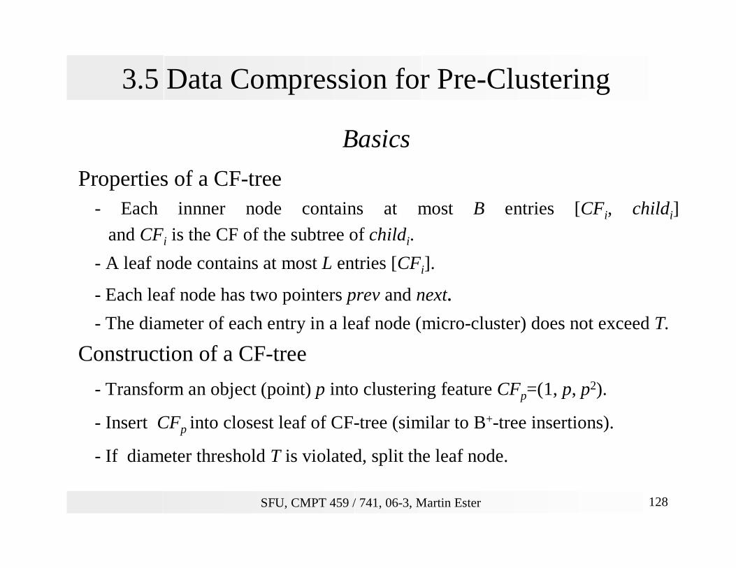
Basics
Properties of a CF-tree- Each innner node contains at most B entries [CFi, childi]
and CFi is the CF of the subtree of childi.
- A leaf node contains at most L entries [CFi].
- Each leaf node has two pointers prev and next.- The diameter of each entry in a leaf node (micro-cluster) does not exceed T.
Construction of a CF-tree
- Transform an object (point) p into clustering feature CFp=(1, p, p2).
- Insert CFp into closest leaf of CF-tree (similar to B+-tree insertions).
- If diameter threshold T is violated, split the leaf node.
SFU, CMPT 459 / 741, 06-3, Martin Ester 129
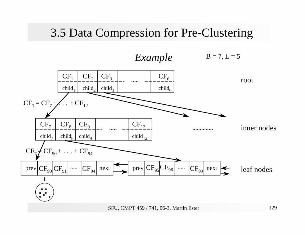
3.5 Data Compression for Pre-Clustering
Example
CF1
child1
CF3
child3
CF2
child2
CF6
child6
CF7
child7
CF9
child9
CF8
child8
CF12
child12
CF90 CF91 CF94prev next CF95 CF96 CF99
prev next
B = 7, L = 5
root
inner nodes
leaf nodes
CF1 = CF7 + . . . + CF12
CF7 = CF90 + . . . + CF94
SFU, CMPT 459 / 741, 06-3, Martin Ester 130
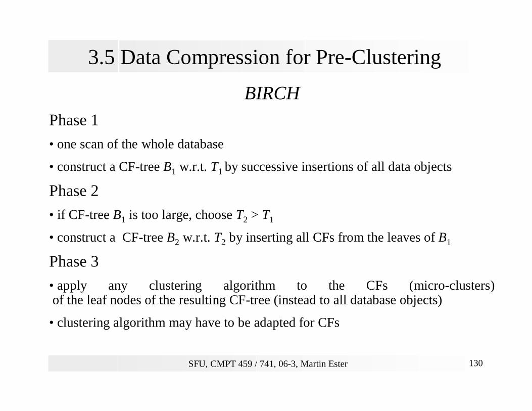
3.5 Data Compression for Pre-Clustering
BIRCH
Phase 1
• one scan of the whole database
• construct a CF-tree B1 w.r.t. T1 by successive insertions of all data objects
Phase 2
• if CF-tree B1 is too large, choose T2 > T1
• construct a CF-tree B2 w.r.t. T2 by inserting all CFs from the leaves of B1
Phase 3
• apply any clustering algorithm to the CFs (micro-clusters)of the leaf nodes of the resulting CF-tree (instead to all database objects)
• clustering algorithm may have to be adapted for CFs
SFU, CMPT 459 / 741, 06-3, Martin Ester 131
3.5 Data Compression for Pre-Clustering
Discussion
+ CF-tree size / compression factor is a user parameter
+ efficiency
construction of secondary storage CF-tree: O(n log n) [page accesses]
construction of main memory CF-tree : O(n) [page accesses]
additionally: cost of clustering algorithm
- only for numeric data Euclidean vector space
- result depends on the order of data objects
SFU, CMPT 459 / 741, 06-3, Martin Ester 132
3.6 Clustering High-Dimensional Data
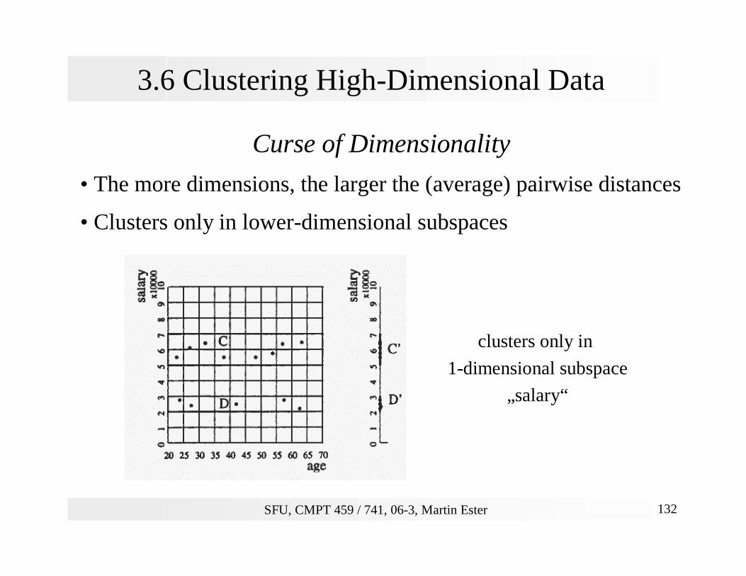
Curse of Dimensionality
• The more dimensions, the larger the (average) pairwise distances
• Clusters only in lower-dimensional subspaces
clusters only in
1-dimensional subspace
„salary“
SFU, CMPT 459 / 741, 06-3, Martin Ester 133
3.6 Subspace Clustering
CLIQUE [Agrawal, Gehrke, Gunopulos & Raghavan 1998]
• Cluster: „dense area“ in dataspace
• Density-threshold
region is dense, if it contains more than objects
• Grid-based approach
each dimension is divided into intervals
cluster is union of connected dense regions (region = grid cell)
• Phases
1. identification of subspaces with clusters
2. identification of clusters
3. generation of cluster descriptions
ττ
ξ
SFU, CMPT 459 / 741, 06-3, Martin Ester 134
3.6 Subspace Clustering
Identification of Subspaces with Clusters
• Task: detect dense base regions
• Naive approach:
calculate histograms for all subsets of the set of dimensions
infeasible for high-dimensional datasets (O (2d) for d dimensions)
• Greedy algorithm (Bottom-Up)
start with the empty set
add one more dimension at a time
• Monotonicity property
if a region R in k-dimensional space is dense, then each projection of R in
(k-1)-dimensional subspace is dense as well (more than objects)τ
SFU, CMPT 459 / 741, 06-3, Martin Ester 135
3.6 Subspace Clustering
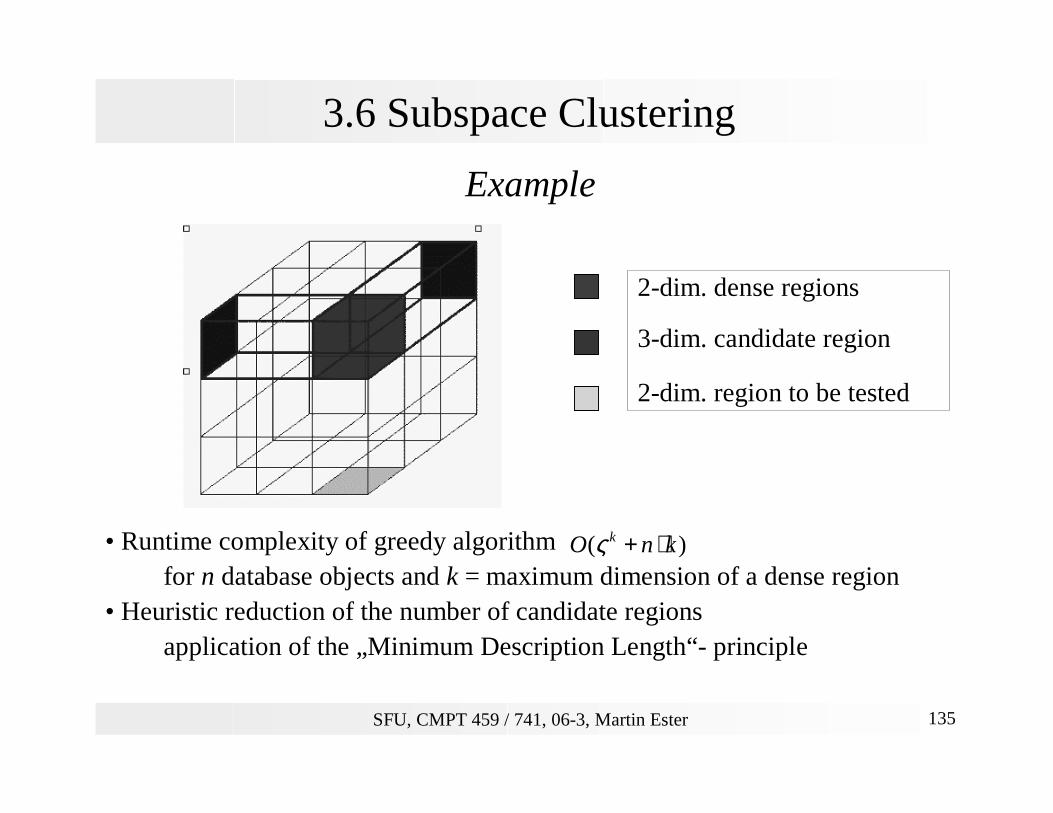
Example
• Runtime complexity of greedy algorithm for n database objects and k = maximum dimension of a dense region
• Heuristic reduction of the number of candidate regionsapplication of the „Minimum Description Length“- principle
2-dim. dense regions
3-dim. candidate region
2-dim. region to be tested
O n kk( )ς + ⋅

SFU, CMPT 459 / 741, 06-3, Martin Ester 136
3.6 Subspace Clustering
Identification of Clusters
• Task: find maximal sets of connected dense base regions
• Given: all dense base regions in a k-dimensional subspace
• „Depth-first“-search of the following graph (search space)
nodes: dense base regions
edges: joint edges / dimensions of the two base regions
• Runtime complexity
dense base regions in main memory (e.g. hash tree)
for each dense base region, test 2 k neighbors
⇒ number of accesses of data structure: 2 k n

SFU, CMPT 459 / 741, 06-3, Martin Ester 137
3.6 Subspace Clustering
Generation of Cluster Descriptions
• Given: a cluster, i.e. a set of connected dense base regions
• Task: find optimal cover of this cluster
by a set of hyperrectangles
• Standard methods
infeasible for large values of d
the problem is NP-complete
• Heuristic method
1. cover the cluster by maximal regions
2. remove redundant regions
SFU, CMPT 459 / 741, 06-3, Martin Ester 138
3.6 Subspace Clustering
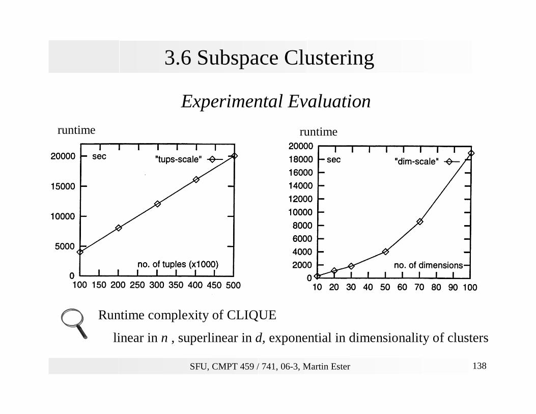
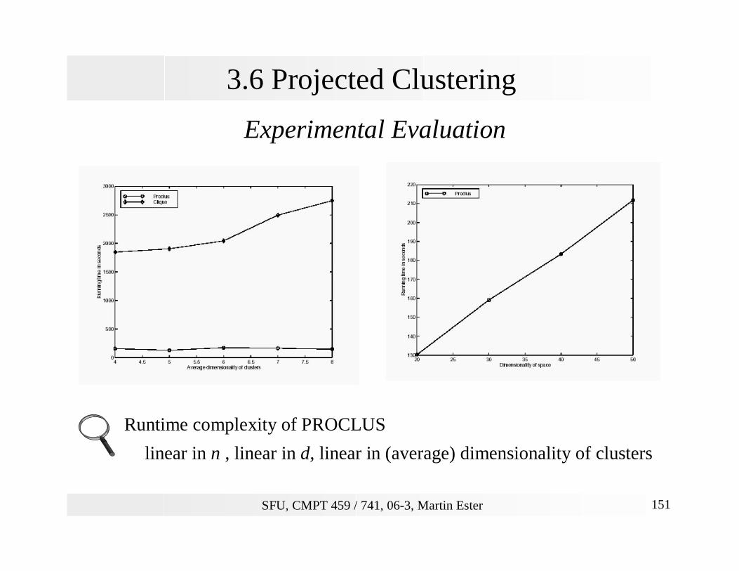
Experimental Evaluation
Runtime complexity of CLIQUE
linear in n , superlinear in d, exponential in dimensionality of clusters
runtime runtime
SFU, CMPT 459 / 741, 06-3, Martin Ester 139
3.6 Subspace Clustering
Discussion
+ Automatic detection of subspaces with clusters
+ No assumptions on the data distribution and number of clusters
+ Scalable w.r.t. the number n of data objects
- Accuracy crucially depends on parameters and
single density threshold for all dimensionalities is problematic
- Needs a heuristics to reduce the search space
method is not complete
ξτ
SFU, CMPT 459 / 741, 06-3, Martin Ester 140
3.6 Subspace Clustering
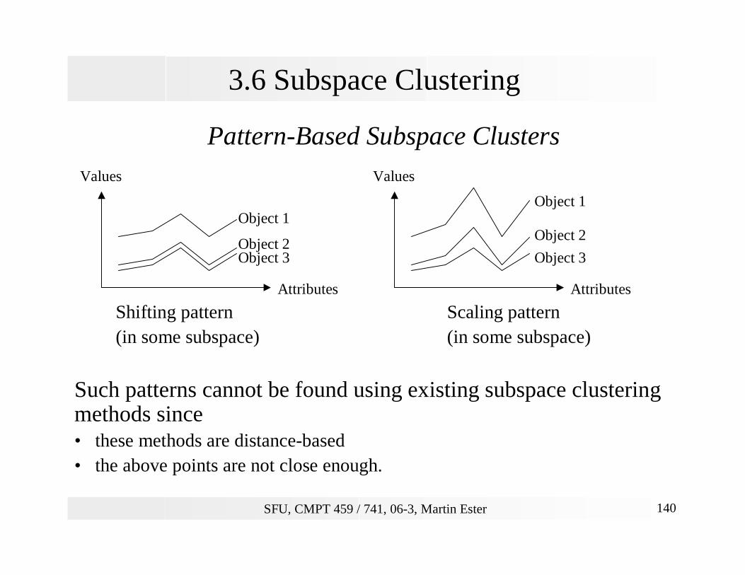
Pattern-Based Subspace Clusters
Shifting pattern Scaling pattern(in some subspace) (in some subspace)
Such patterns cannot be found using existing subspace clusteringmethods since• these methods are distance-based • the above points are not close enough.
Attributes
Values
Attributes
Values
Object 1
Object 2Object 3
Object 1
Object 2
Object 3
SFU, CMPT 459 / 741, 06-3, Martin Ester 141
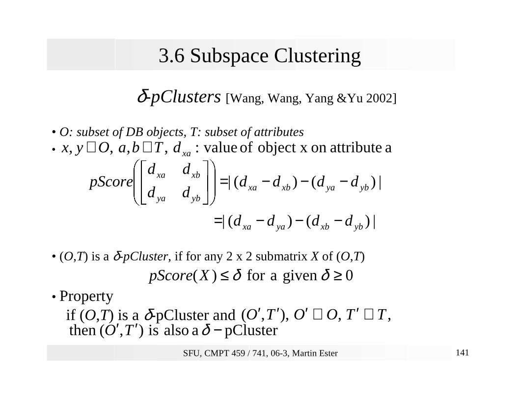
3.6 Subspace Clustering
δ-pClusters [Wang, Wang, Yang &Yu 2002]
• O: subset of DB objects, T: subset of attributes •
• (O,T) is a δ-pCluster, if for any 2 x 2 submatrix X of (O,T)
• Propertyif (O,T) is a δ-pCluster and
a attributeon object x of value:,,,, xadTbaOyx ∈∈
|)()(|
|)()(|
ybxbyaxa
ybyaxbxaybya
xbxa
dddd
dddddd
ddpScore
−−−=
−−−=
0given afor)( ≥≤ δδXpScore
pClustera alsois),(then −′′ δTO,,),,( TTOOTO ⊆′⊆′′′

SFU, CMPT 459 / 741, 06-3, Martin Ester 142
3.6 Subspace Clustering
Problem
• Given δ , nc (minimal number of columns), nr (minimal number of rows), find all pairs (O,T) such that
• (O,T) is a δ−pCluster•
•
• For δ−pCluster (O,T), T is a Maximum Dimension Set if there does not exist
•
• Objects x and y form a δ−pCluster on T iff the difference between the largest and smallest value in S(x,y,T) is below δ
nrO ≥||ncT ≥||
pCluster- a also is ),(such that δTOTT ′⊃′
}|{),,( TaddTyxS yaxa ∈−=

SFU, CMPT 459 / 741, 06-3, Martin Ester 143
3.6 Subspace Clustering
Algorithm
•
• Given A, is a MDS of x and y iff
and
• Pairwise clustering of x and y:
compute
identify all subsequences with the above property
Ex.: -3 -2 -1 6 6 7 8 8 10, δ = 2
δδδ >−>−≤− −+ 11 and, ijijij ssssss
jiTyxSssTyxS jiik <≤∈= for ss and ),,(s where,...,),,( 1
r
AT ⊆),,( of esubsequenc contiguous a is...),,( AyxSssTyxS ji
rr
=
),,( TyxSr
SFU, CMPT 459 / 741, 06-3, Martin Ester 144
3.6 Subspace Clustering
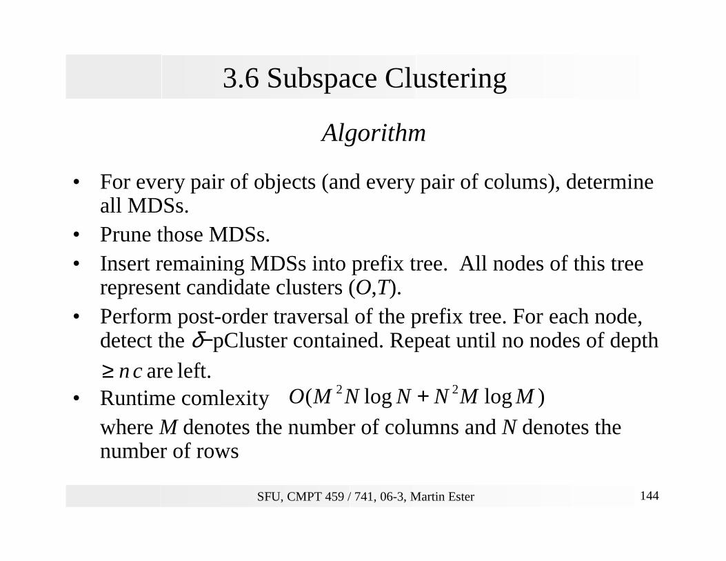
Algorithm
• For every pair of objects (and every pair of colums), determine all MDSs.
• Prune those MDSs.• Insert remaining MDSs into prefix tree. All nodes of this tree
represent candidate clusters (O,T).• Perform post-order traversal of the prefix tree. For each node,
detect the δ−pCluster contained. Repeat until no nodes of depth
• Runtime comlexitywhere M denotes the number of columns and N denotes the number of rows
left. are cn≥)loglog( 22 MMNNNMO +
SFU, CMPT 459 / 741, 06-3, Martin Ester 145
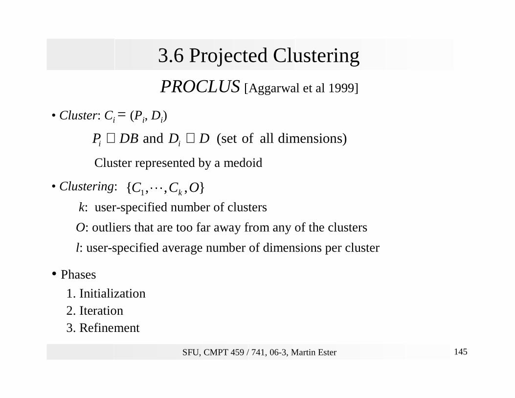
3.6 Projected Clustering
PROCLUS [Aggarwal et al 1999]
• Cluster: Ci = (Pi, Di)
Cluster represented by a medoid
• Clustering:
k: user-specified number of clusters
O: outliers that are too far away from any of the clusters
l: user-specified average number of dimensions per cluster
• Phases
1. Initialization2. Iteration3. Refinement
)dimensionsallof(setand DDDBP ii ⊆⊆
},,,{ 1 OCC kL
SFU, CMPT 459 / 741, 06-3, Martin Ester 146
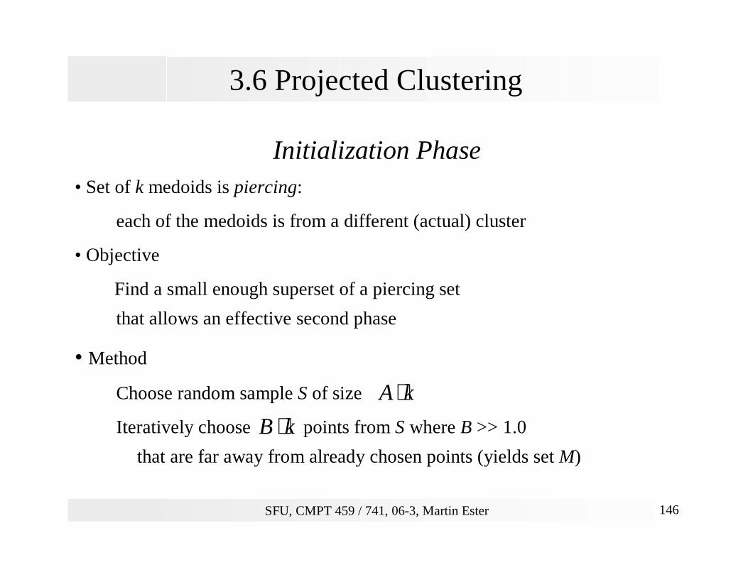
3.6 Projected Clustering
Initialization Phase• Set of k medoids is piercing:
each of the medoids is from a different (actual) cluster
• Objective
Find a small enough superset of a piercing set
that allows an effective second phase
• Method
Choose random sample S of size
Iteratively choose points from S where B >> 1.0
that are far away from already chosen points (yields set M)
kA ⋅kB ⋅
SFU, CMPT 459 / 741, 06-3, Martin Ester 147
3.6 Projected Clustering
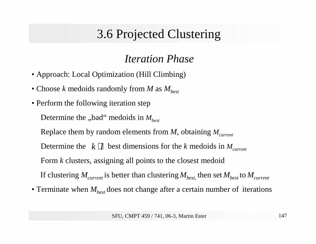
Iteration Phase• Approach: Local Optimization (Hill Climbing)
• Choose k medoids randomly from M as Mbest
• Perform the following iteration step
Determine the „bad“ medoids in Mbest
Replace them by random elements from M, obtaining Mcurrent
Determine the best dimensions for the k medoids in Mcurrent
Form k clusters, assigning all points to the closest medoid
If clustering Mcurrent is better than clustering Mbest, then set Mbest to Mcurrent
• Terminate when Mbest does not change after a certain number of iterations
lk ⋅
SFU, CMPT 459 / 741, 06-3, Martin Ester 148
3.6 Projected Clustering
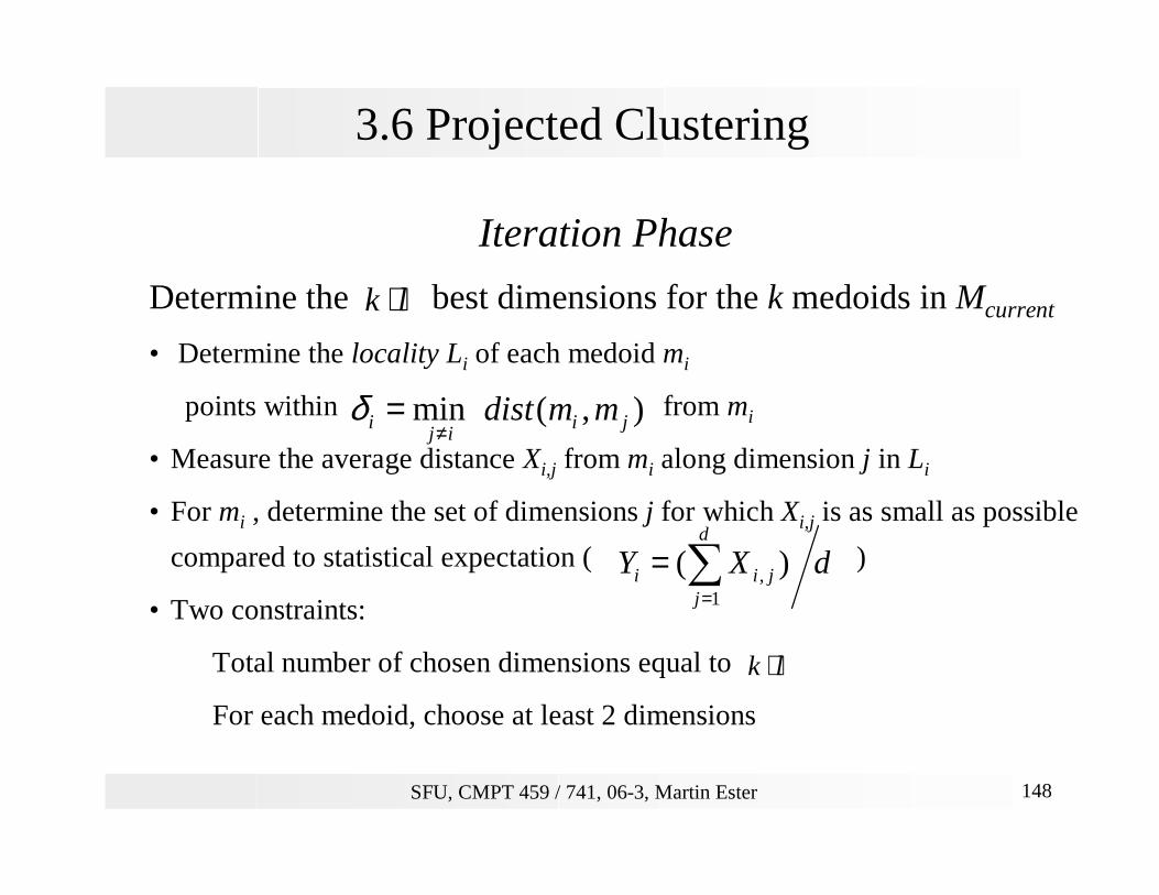
Iteration Phase
Determine the best dimensions for the k medoids in Mcurrent
• Determine the locality Li of each medoid mi
points within from mi
• Measure the average distance Xi,j from mi along dimension j in Li
• For mi , determine the set of dimensions j for which Xi,j is as small as possible
compared to statistical expectation ( )
• Two constraints:
Total number of chosen dimensions equal to
For each medoid, choose at least 2 dimensions
lk ⋅
),(min jiij
i mmdist≠
=δ
dXYd
jjii ∑
=
=1
, )(
lk ⋅
SFU, CMPT 459 / 741, 06-3, Martin Ester 149
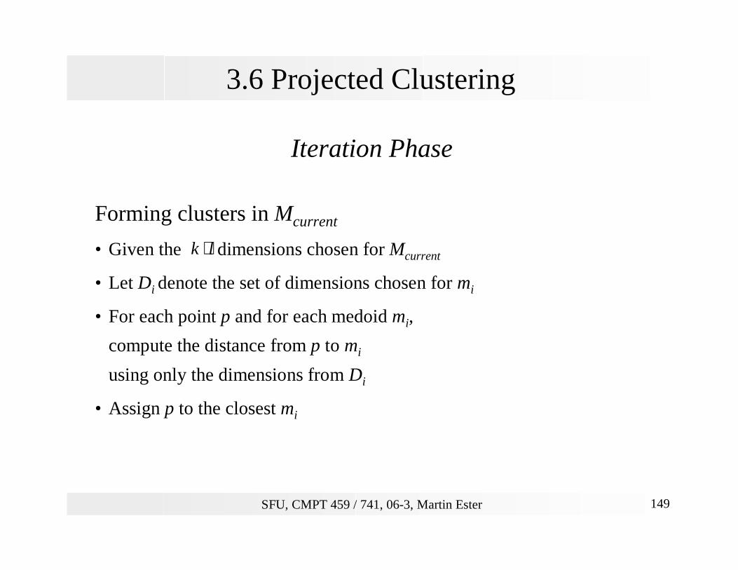
3.6 Projected Clustering
Iteration Phase
Forming clusters in Mcurrent
• Given the dimensions chosen for Mcurrent
• Let Di denote the set of dimensions chosen for mi
• For each point p and for each medoid mi,
compute the distance from p to mi
using only the dimensions from Di
• Assign p to the closest mi
lk ⋅
SFU, CMPT 459 / 741, 06-3, Martin Ester 150
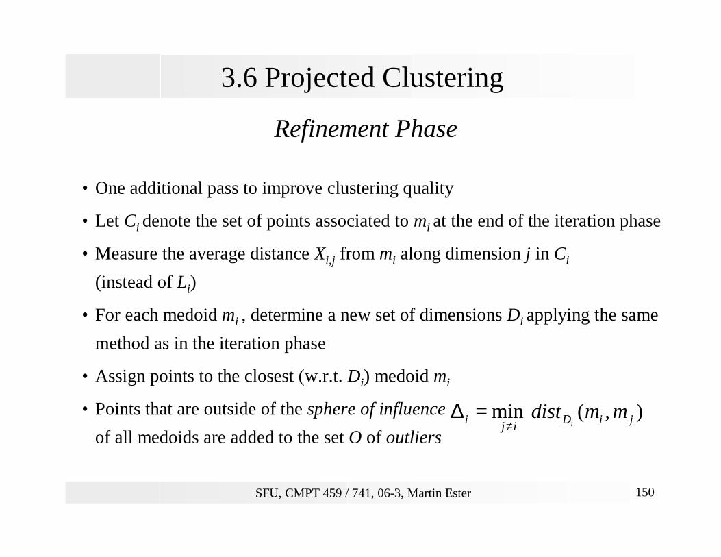
3.6 Projected Clustering
Refinement Phase
• One additional pass to improve clustering quality
• Let Ci denote the set of points associated to mi at the end of the iteration phase
• Measure the average distance Xi,j from mi along dimension j in Ci
(instead of Li)
• For each medoid mi , determine a new set of dimensions Di applying the same
method as in the iteration phase
• Assign points to the closest (w.r.t. Di) medoid mi
• Points that are outside of the sphere of influence
of all medoids are added to the set O of outliers
),(min jiDij
i mmdisti≠
=∆
SFU, CMPT 459 / 741, 06-3, Martin Ester 151
3.6 Projected Clustering
Experimental Evaluation
Runtime complexity of PROCLUS
linear in n , linear in d, linear in (average) dimensionality of clusters
SFU, CMPT 459 / 741, 06-3, Martin Ester 152
3.6 Projected Clustering
Discussion+ Automatic detection of subspaces with clusters
+ No assumptions on the data distribution
+ Output easier to interpret than that of subspace clustering
+ Scalable w.r.t. the number n of data objects, d of dimensions and the average
cluster dimensionality l
- Finds only one (of the many possible) clusterings
- Finds only spherical clusters
- Clusters must have similar dimensionalities
- Accuracy very sensitive to the parameters k and l
parameter values hard to determine a priori
SFU, CMPT 459 / 741, 06-3, Martin Ester 153
3.7 Outlier Detection
Overview
Definition
Outliers: objects significantly dissimilar from the remainder of the data
Applications
• Credit card fraud detection
• Telecom fraud detection
• Medical analysis
Problem
• Find top k outlier points
SFU, CMPT 459 / 741, 06-3, Martin Ester 154
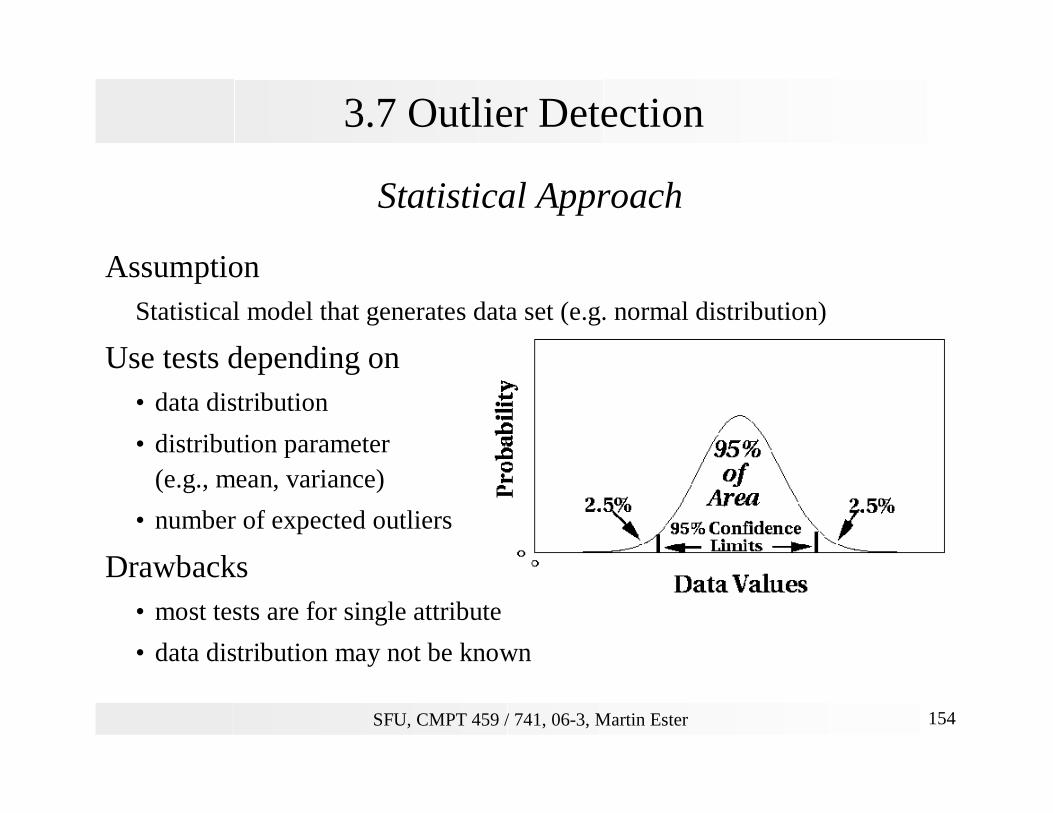
3.7 Outlier Detection
Statistical Approach
AssumptionStatistical model that generates data set (e.g. normal distribution)
Use tests depending on • data distribution
• distribution parameter (e.g., mean, variance)
• number of expected outliers
Drawbacks• most tests are for single attribute
• data distribution may not be known
SFU, CMPT 459 / 741, 06-3, Martin Ester 155
3.7 Outlier Detection
Distance-Based Approach
Ideaoutlier analysis without knowing data distribution
DefinitionDB(p, t)-outlier:
object o in a dataset D such that at least a fraction p of the objects in D has a distance greater than t from o
Algorithms for mining distance-based outliers • Index-based algorithm
• Nested-loop algorithm
• Cell-based algorithm
SFU, CMPT 459 / 741, 06-3, Martin Ester 156
3.7 Outlier Detection
Deviation-Based ApproachIdea
• Identifies outliers by examining the main characteristics of objects in a group
• Objects that “deviate” from this description are considered outliers
Sequential exception technique • simulates the way in which humans can distinguish unusual objects from
among a series of supposedly like objects
OLAP data cube technique• uses data cubes to identify regions of anomalies in large multidimensional
data
• Example: city with significantly higher sales increase than its region