3. Classical Physics in Galilean and Minkowski Spacetimes

3.1. The Action Principle in Galilean Spacetime3.2. Symmetries and Conservation Laws3.3. The Hamiltonian3.4. Poisson Brackets and Translation Operators3.5. The Action Principle in Minkowski Spacetime3.6. Classical Electrodynamics3.7. Geometry in Classical Physics

Purpose: Set out classical mechanics in a form suitable for generalization to general relativity & quantum mechanics.

Two basic ideas:

1. Action (contains all dynamical information of the system ).

2. Symmetry ~ conservation law.

Comment:

Not all systems can be described by an action, e.g. systems with dissipation.

However, all known fundamental (microscopic) interaction can.

3.1. The Action Principle in Galilean Spacetime

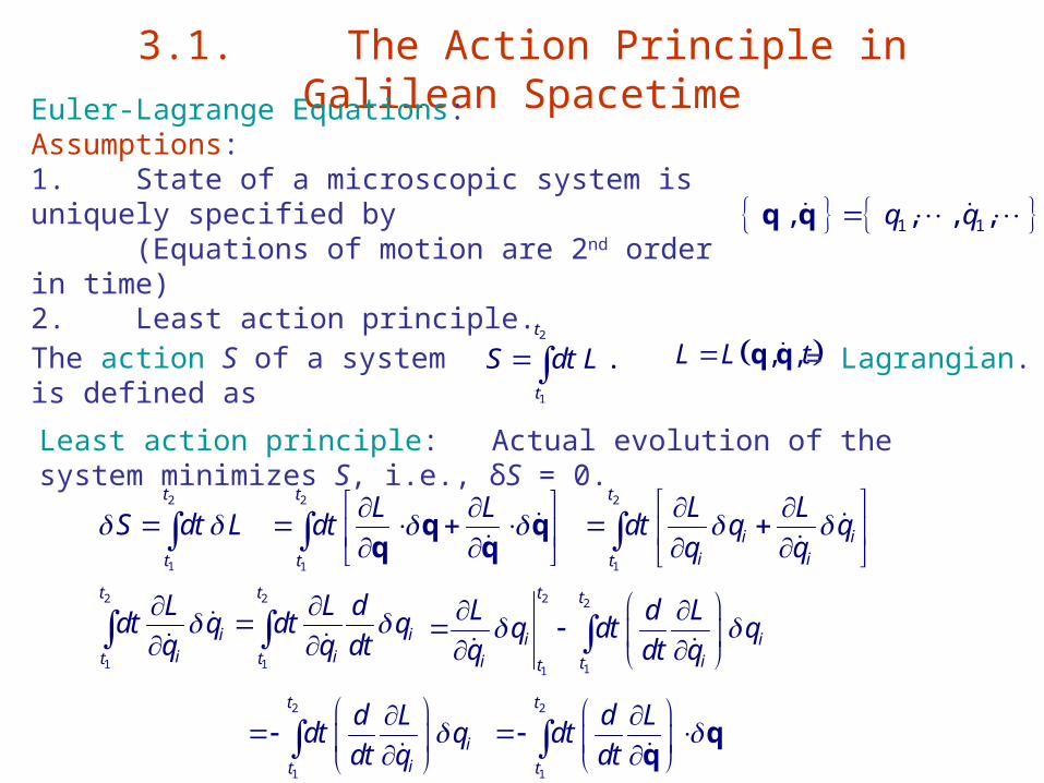
Euler-Lagrange Equations:Assumptions:1. State of a microscopic system is uniquely specified by (Equations of motion are 2nd order in time)2. Least action principle.

The action S of a system is defined as2

1

.t

t

S dt L

1 1, , , ,q qq q

, ,L L t q q = Lagrangian.

Least action principle: Actual evolution of the system minimizes S, i.e., δS = 0.

2

1

t

t

S dt L 2

1

t

t

L Ldt

q q

q q

2

1

t

i ii it

L Ldt q q

q q

2 2

1 1

t t

i ii it t

L L ddt q dt q

q q dt

2 2

11

t t

i ii itt

L d Lq dt q

q dt q

2

1

t

iit

d Ldt q

dt q

2

1

t

t

d Ldt

dt

q

q

2

1

0t

ii it

L d LS dt q

q dt q

0i i

L d L

q dt q

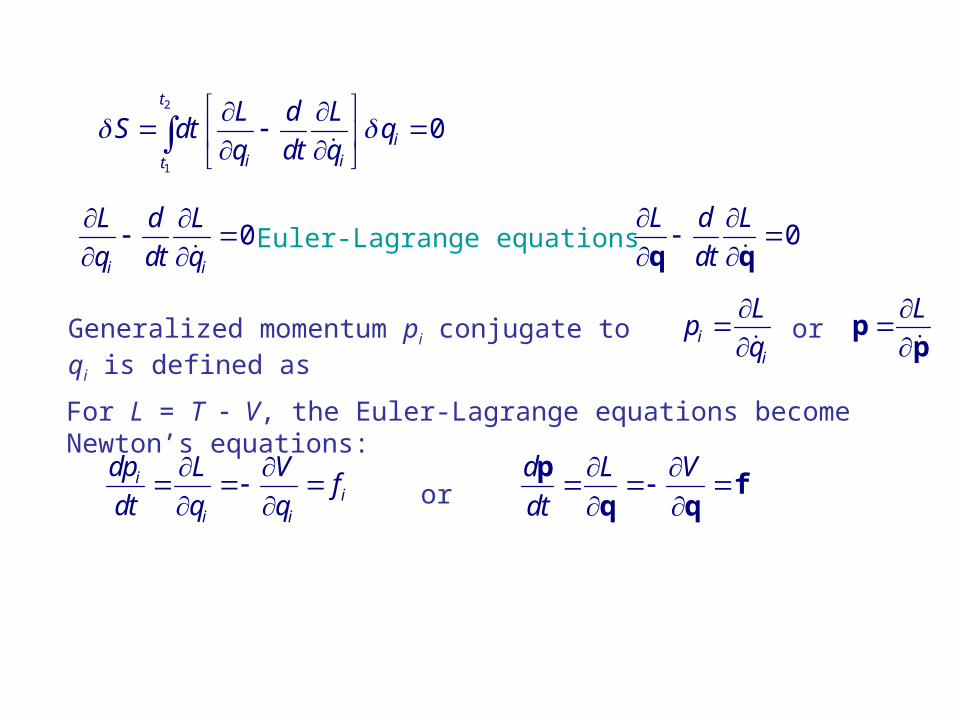
Euler-Lagrange equations

Generalized momentum pi conjugate to qi is defined as ii

Lp

q

0L d L

dt

q q

L

pp

For L = T V, the Euler-Lagrange equations become Newton’s equations:

ii

i i

dp L Vf

dt q q

or

ord L V

dt

pf

q q

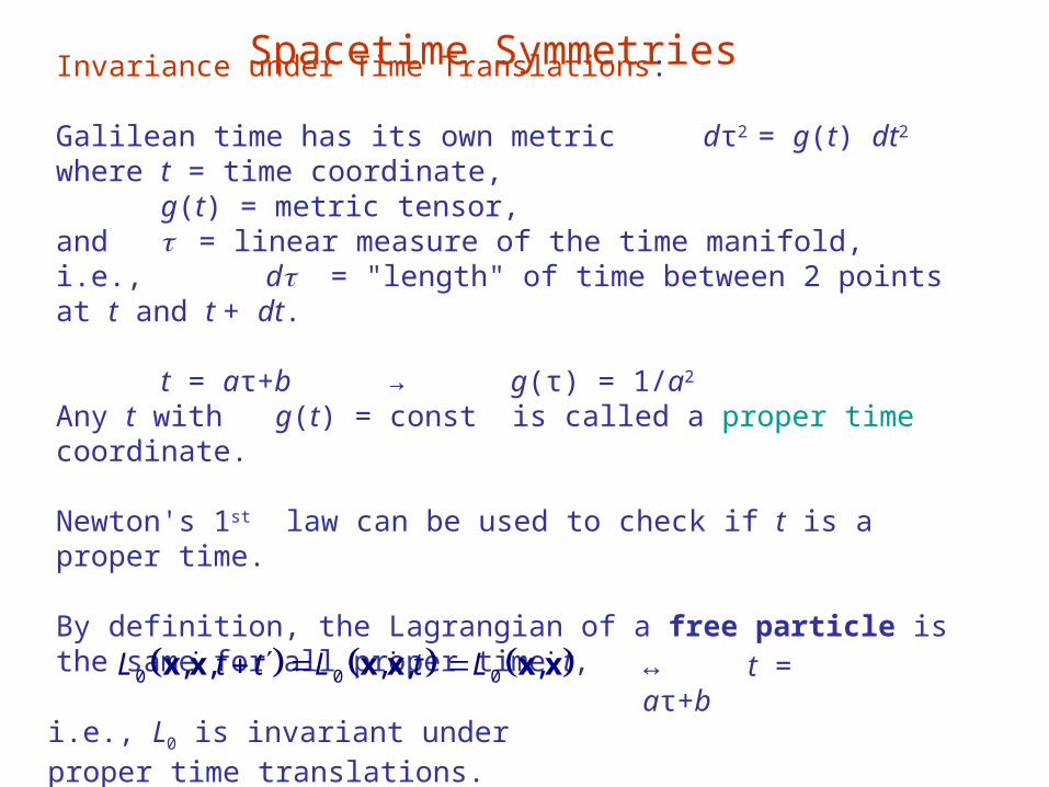
Spacetime Symmetries

Invariance under Time Translations:

Galilean time has its own metric dτ2 = g(t) dt2 where t = time coordinate,

g(t) = metric tensor,and = linear measure of the time manifold,i.e., d = "length" of time between 2 points at t and t + dt.

t = aτ+b → g(τ) = 1/a2

Any t with g(t) = const is called a proper time coordinate.

Newton's 1st law can be used to check if t is a proper time.

By definition, the Lagrangian of a free particle is the same for all proper time t,

i.e., L0 is invariant under proper time translations.

0 0, , , ,L t t L t x x x x 0 ,L x x ↔ t = aτ+b

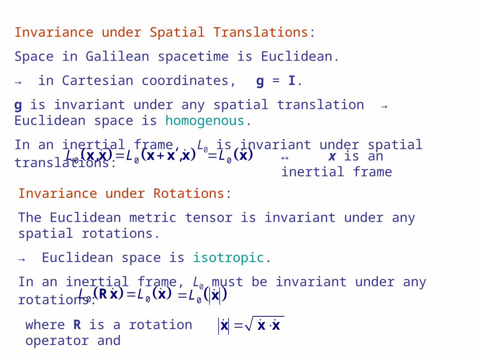
Invariance under Spatial Translations:

Space in Galilean spacetime is Euclidean.

→ in Cartesian coordinates, g = I.

g is invariant under any spatial translation → Euclidean space is homogenous.

In an inertial frame, L0 is invariant under spatial translations:

0 0, ,L L x x x x x 0L x ↔ x is an inertial frame

Invariance under Rotations:

The Euclidean metric tensor is invariant under any spatial rotations.

→ Euclidean space is isotropic.

In an inertial frame, L0 must be invariant under any rotations:

0 0L LRx x 0L x

where R is a rotation operator and x x x

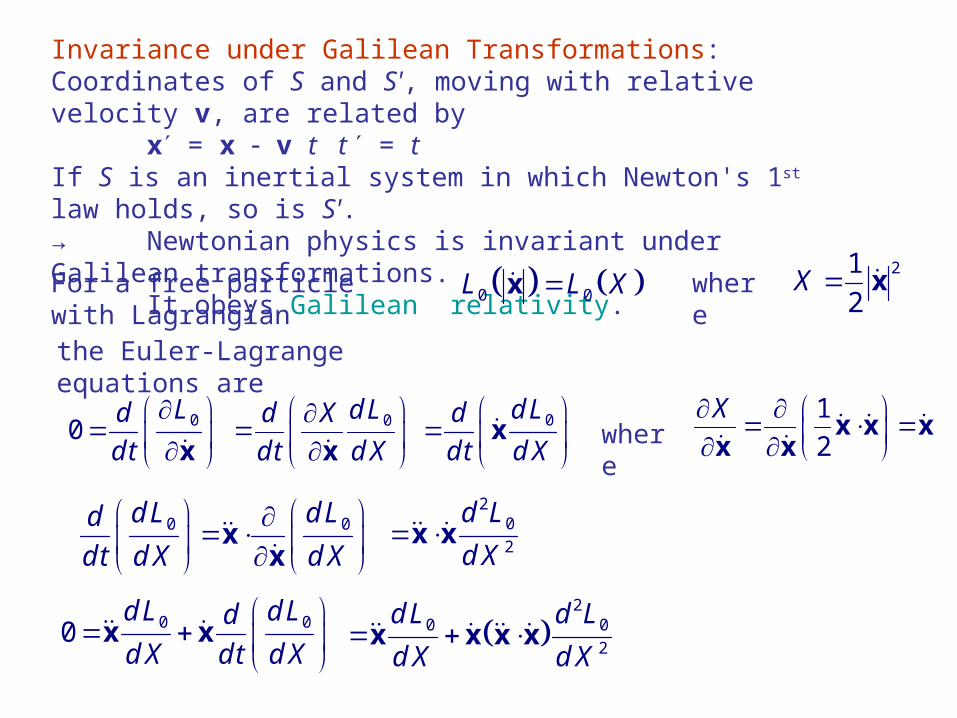
Invariance under Galilean Transformations:Coordinates of S and S', moving with relative velocity v, are related by

x = x v t t = tIf S is an inertial system in which Newton's 1st law holds, so is S'. → Newtonian physics is invariant under Galilean transformations.

It obeys Galilean relativity.

For a free particle with Lagrangian 0 0L L Xx21

2X xwhere

the Euler-Lagrange equations are

00Ld

d t

x

0d Ld X

dt d X

x

0d Ld

d t d X

x

1

2

X x x x

x x

where

0 0d L d Ld

d t d X d X

xx

20

2

d L

d X x x

0 00d L d Ld

d X d t d X

x x

20 0

2

d L d L

d X d X x x x x

2

0 0

20

d L d L

d X d X x x x x

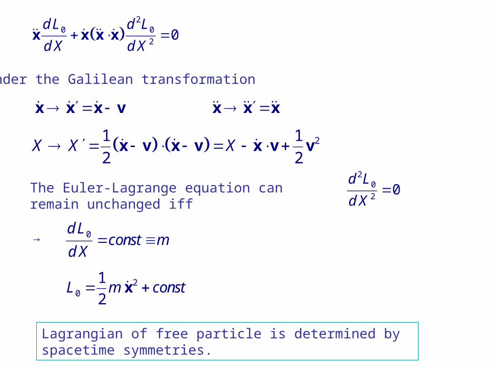
Under the Galilean transformation

x x x v x x x

21 1

2 2X X X x v x v x v v

The Euler-Lagrange equation can remain unchanged iff2

0

20

d L

d X

→ 0d Lconst m

d X

20

1

2L m const x

Lagrangian of free particle is determined by spacetime symmetries.

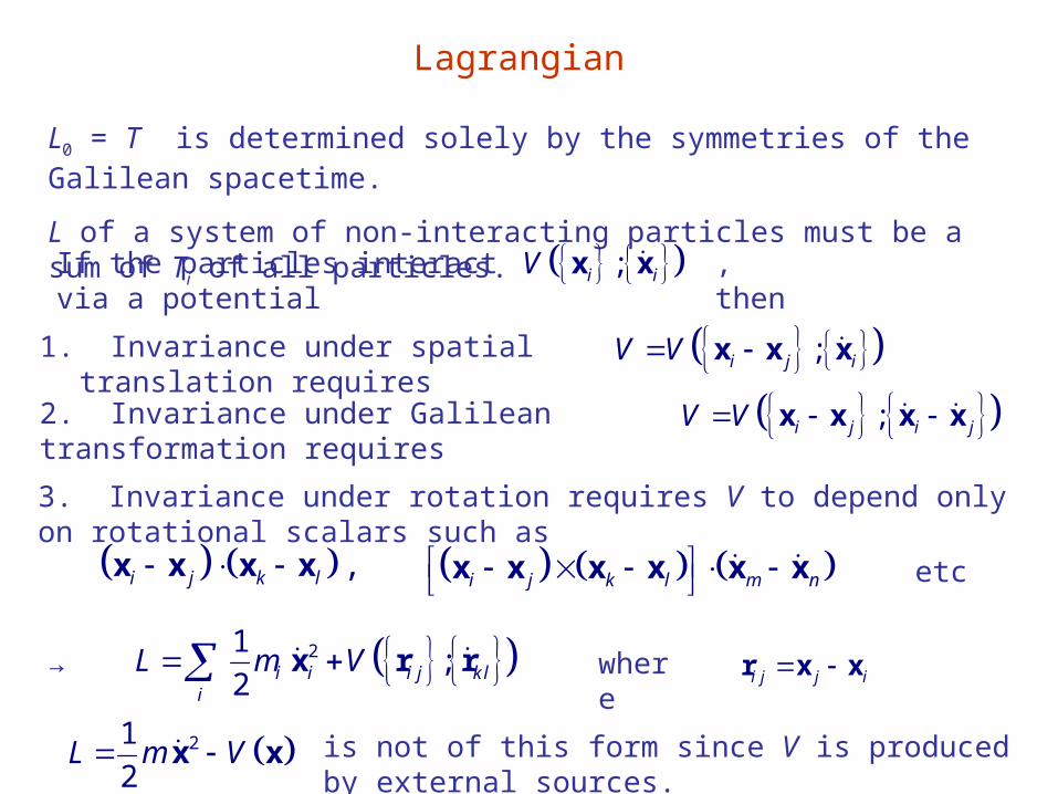
Lagrangian

L0 = T is determined solely by the symmetries of the Galilean spacetime.

L of a system of non-interacting particles must be a sum of Ti of all particles.

If the particles interact via a potential ;i iV x x

1. Invariance under spatial translation requires

, then

;i j iV V x x x

2. Invariance under Galilean transformation requires ;i j i jV V x x x x

3. Invariance under rotation requires V to depend only on rotational scalars such as

,i j k l x x x x i j k l m n x x x x x x etc

21;

2 i i i j k li

L m V x r r→ where i j j i r x x

21

2L m V x x is not of this form since V is produced by external sources.

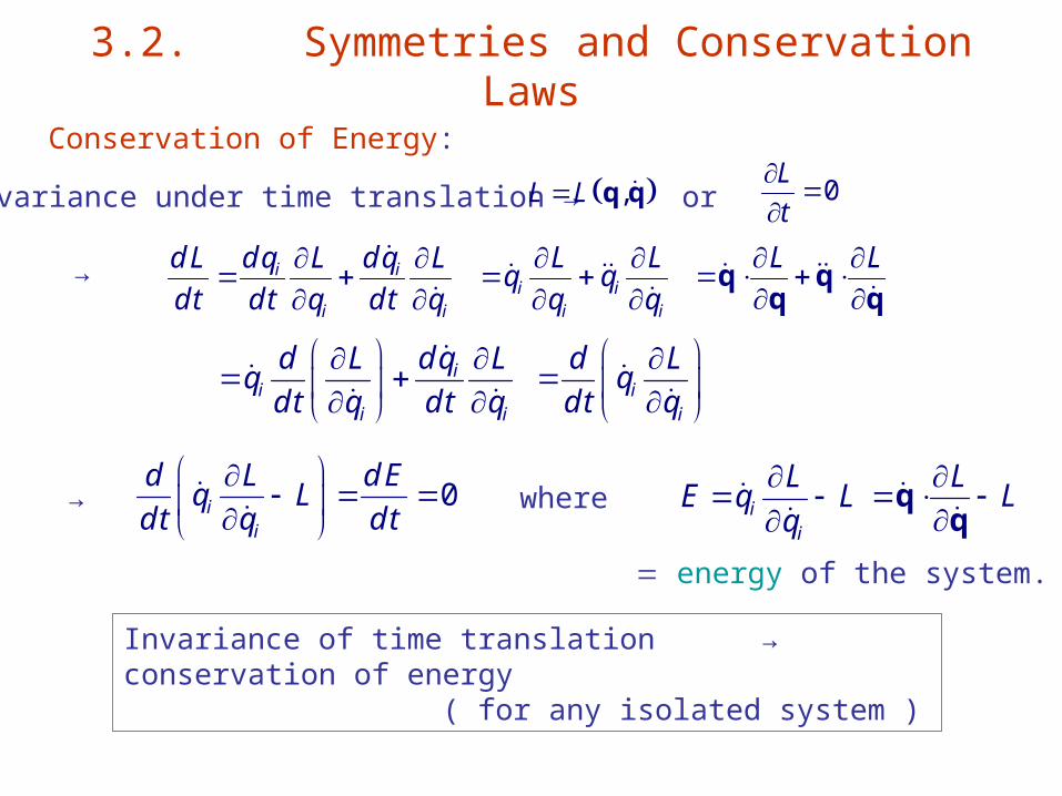
3.2. Symmetries and Conservation Laws

Conservation of Energy:

Invariance under time translation → ,L L q q 0L

t

or

→ i i

i i

d L d q L d q L

d t d t q d t q

i ii i

L Lq q

q q

L L

q qq q

i

ii i

d L d q Lq

d t q d t q

ii

d Lq

d t q

0ii

d L d Eq L

d t q d t

→ i

i

LE q L

q

L

L

qq

where

energy of the system.

Invariance of time translation → conservation of energy ( for any isolated system )

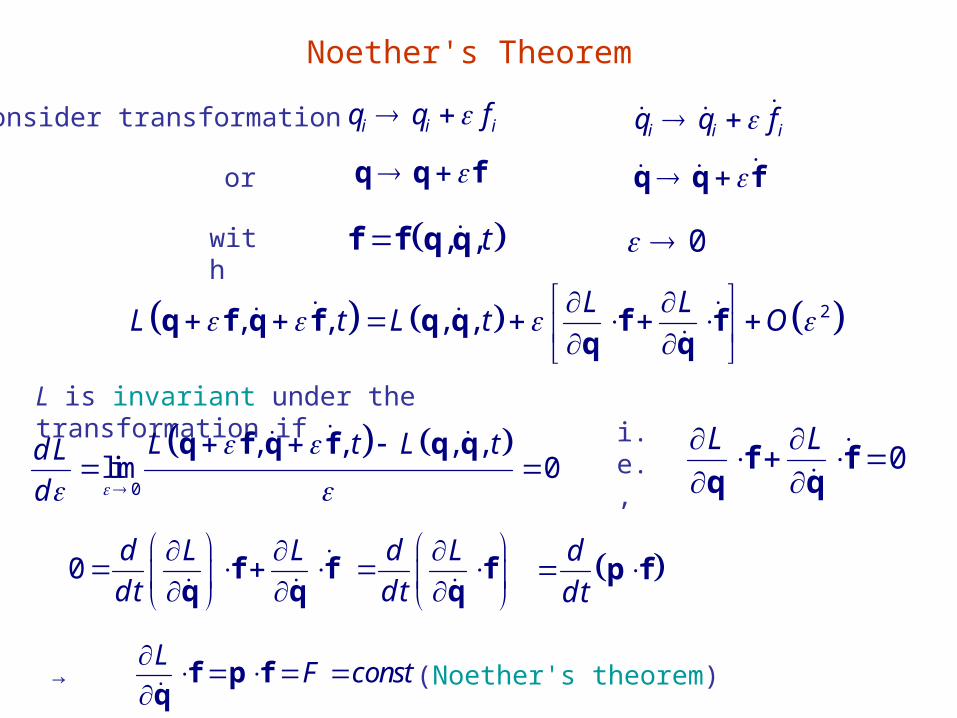
Noether's Theorem

Consider transformation i i iq q f i i iq q f

q q f q q for

, , tf f q q 0 with

2, , , ,L L

L t L t O

q f q f q q f f

q q

L is invariant under the transformation if

0

, , , ,lim 0

L t L td L

d

q f q f q qi.e., 0

L L

f f

q q

0d L L

d t

f fq q

d

d t p f

LF const

f p f

q

(Noether's theorem)→

d L

d t

fq

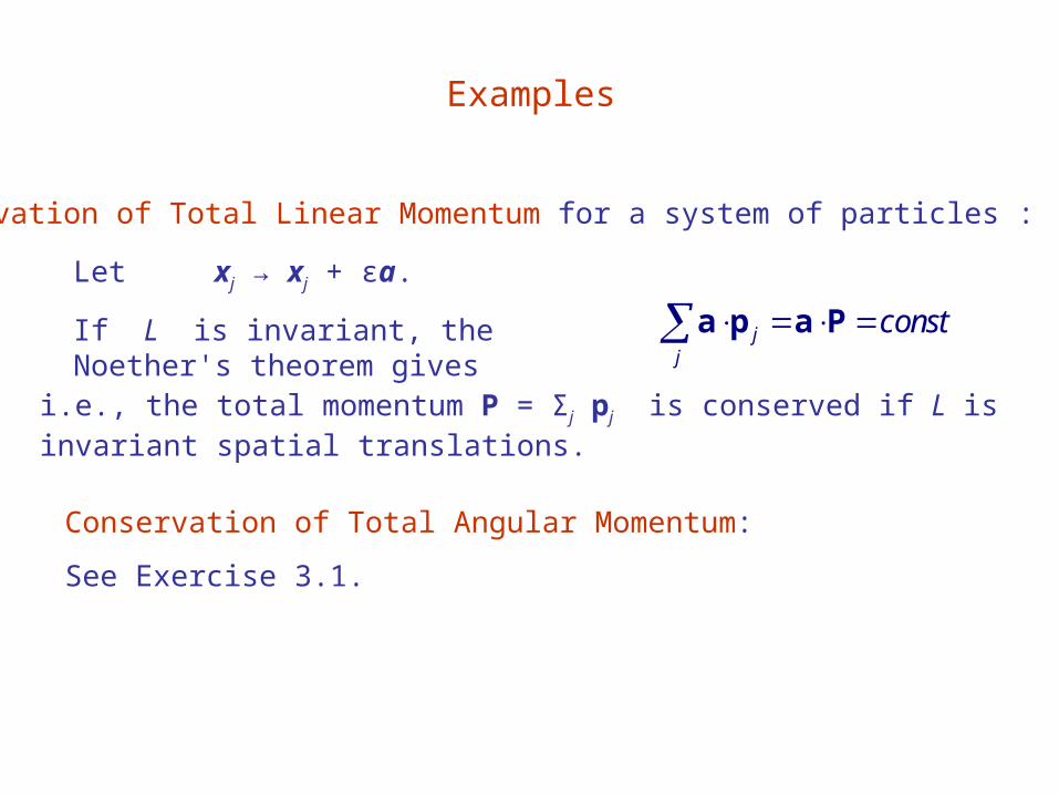
Examples

Let xj → xj + εa.

If L is invariant, the Noether's theorem gives jj

const a p a P

Conservation of Total Linear Momentum for a system of particles :

i.e., the total momentum P = Σj pj is conserved if L is invariant spatial translations.

Conservation of Total Angular Momentum:

See Exercise 3.1.

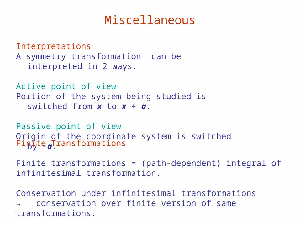
Miscellaneous

InterpretationsA symmetry transformation can be interpreted in 2 ways.

Active point of viewPortion of the system being studied is switched from x to x + a.

Passive point of viewOrigin of the coordinate system is switched by –a.

Finite Transformations

Finite transformations = (path-dependent) integral of infinitesimal transformation. Conservation under infinitesimal transformations → conservation over finite version of same transformations.

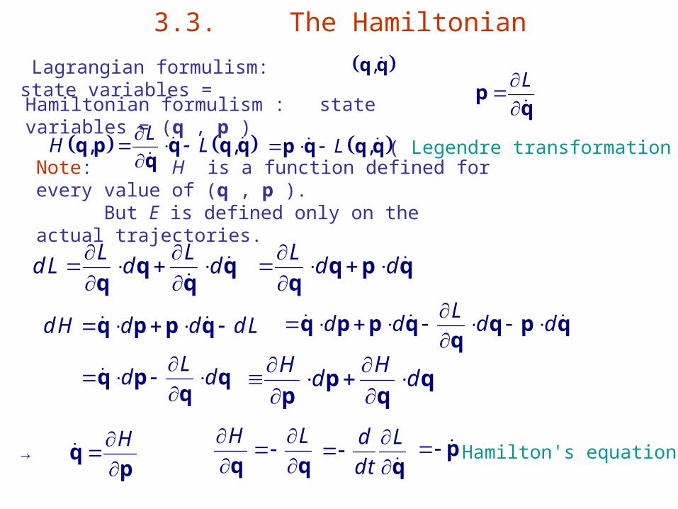
3.3. The Hamiltonian

Lagrangian formulism: state variables =

,q q

Hamiltonian formulism : state variables = (q , p )

, ,L

H L

q p q q qq

,L p q q q

( Legendre transformation )

L

p

q

Note: H is a function defined for every value of (q , p ).But E is defined only on the actual trajectories.

L Ld L d d

q q

q q

L

d d

q p qq

d H d d d L q p p qL

d d d d

q p p q q p qq

Ld d

q p q

q

H Hd d

p q

p q

→H

qp

H L

q q

d L

d t

q p

Hamilton's equations

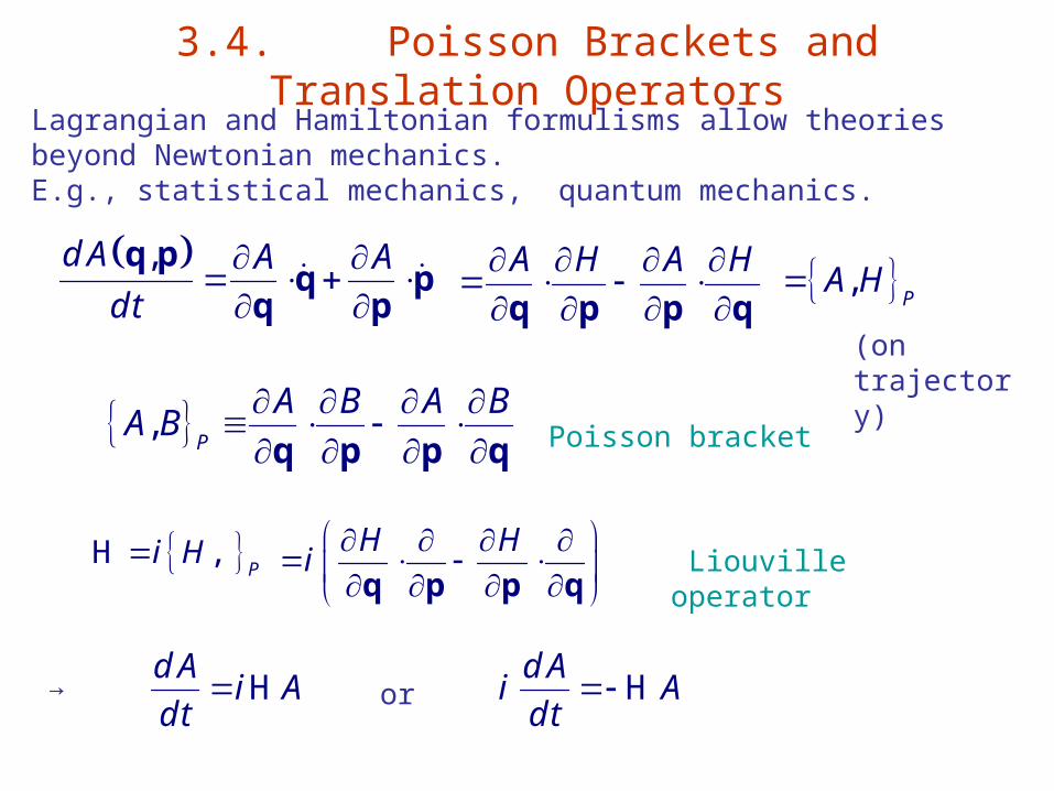
3.4. Poisson Brackets and Translation OperatorsLagrangian and Hamiltonian formulisms allow theories beyond Newtonian mechanics.E.g., statistical mechanics, quantum mechanics.

,d A A A

dt

q p

q pq p

A H A H

q p p q ,

PA H

,P

A B A BA B

q p p q Poisson bracket

(on trajectory)

,P

i HH H Hi

q p p q

→d A

i Ad t

Hd A

i Ad t

H

or

Liouville operator

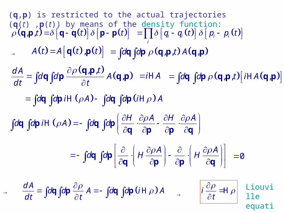
(q,p) is restricted to the actual trajectories (q(t) ,p(t)) by means of the density function:

, , t t t q p q q p p i i i ii

q q t p p t ,A t A t t q p , , ,d d t A q p q p q p→

, ,,

td Ad d A

d t t

q p

q p q p i A H , , ,d d t i A q p q p q pH

d d i A d d i A q p q pH H

H A H Ad d i A d d

q p q pq p p q

H

A Ad d H H

q pq p p q

0

→ d Ad d A d d i A

d t t

q p q p H it

H Liouville

equation→

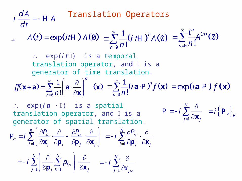
Translation Operators d Ai A

d t H

→ exp 0A t it A H 0

10

!n

n

i t An

H

0

0!

nn

n

tA

n

exp(i t ) is a temporal translation operator, and is a generator of time translation.

0

1

!

n

n

f fn

x a a xx

0

1

!

n

n

i fn

a xP =exp i fa xP

exp(i a · ) is a spatial translation operator, and is a generator of spatial translation. 1

N

j j

i

xP ,

Pi P

1

n

j j j j j

P Pi

x p p xP

1

N

j j j

Pi

p x

1 1

N N

kj kj j

i p

p x 1

N

j j

ix

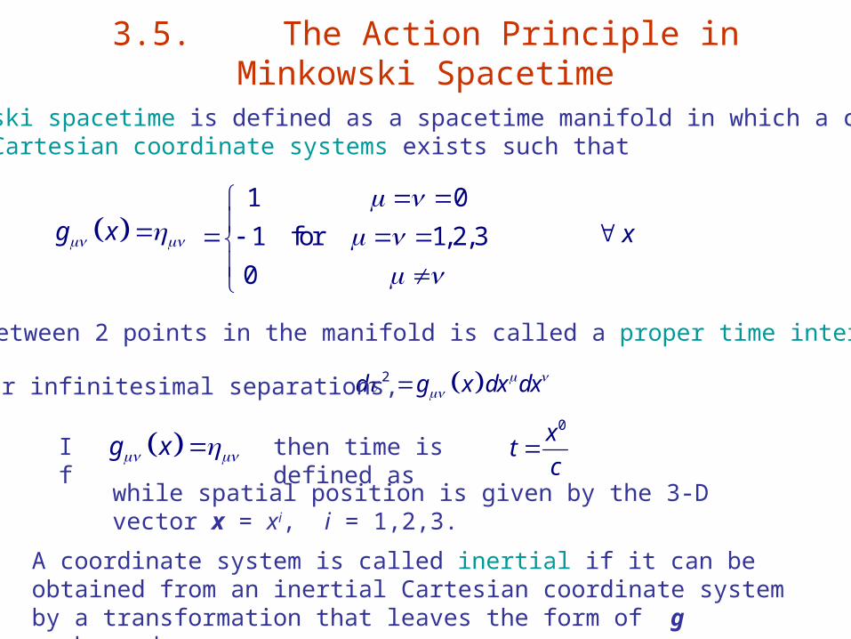
3.5. The Action Principle in Minkowski Spacetime

2d g x dx dx

g x

A Minkowski spacetime is defined as a spacetime manifold in which a class of inertial Cartesian coordinate systems exists such that

x1 0

1 for 1,2,3

0

Distance between 2 points in the manifold is called a proper time interval, .

For infinitesimal separations,

g x If then time is defined as 0x

tc

while spatial position is given by the 3-D vector x = xi, i = 1,2,3.

A coordinate system is called inertial if it can be obtained from an inertial Cartesian coordinate system by a transformation that leaves the form of g unchanged.

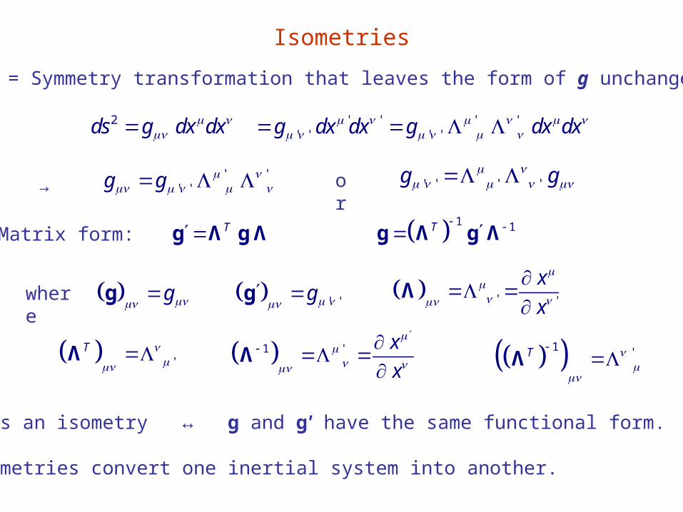
Isometries

Isometry = Symmetry transformation that leaves the form of g unchanged.

2ds g dx dx ' '

' 'g dx dx

' '' 'g dx dx

→' '

' 'g g or ' ' ' 'g g

Matrix form: 1 1T g Λ g ΛTg Λ g Λ

where g

g ' 'g g ' '

x

x

Λ

'T

Λ

Λ is an isometry ↔ g and g' have the same functional form. Isometries convert one inertial system into another.

1 ' x

x

Λ 1 'T

Λ

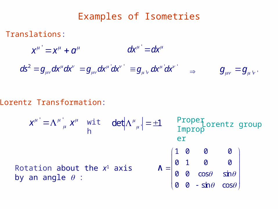
Examples of Isometries

Translations:

'x x a 'dx dx

2ds g dx dx ' 'g dx dx

' '' 'g dx dx

' 'g g

Lorentz Transformation:

' 'x x Proper

Improper'det 1 with

Rotation about the x1 axis by an angle :

1 0 0 0

0 1 0 0

0 0 cos sin

0 0 sin cos

Λ

Lorentz group

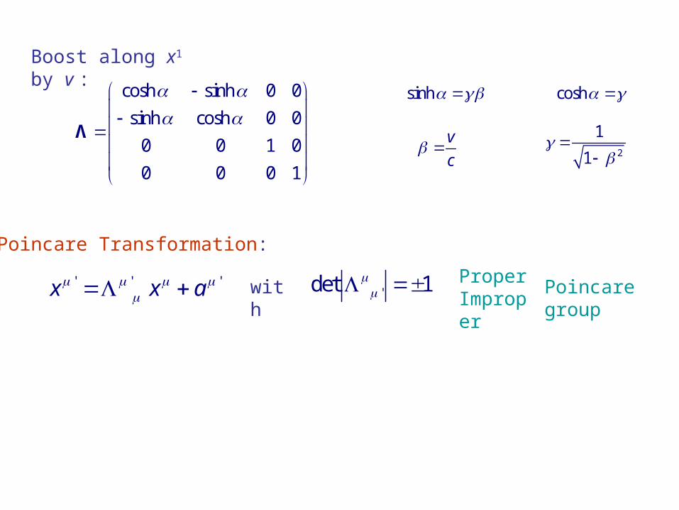
Poincare Transformation:

' ' 'x x a Poincare

group'det 1

with

Boost along x1 by v :

cosh sinh 0 0

sinh cosh 0 0

0 0 1 0

0 0 0 1

Λ

sinh cosh

v

c 2

1

1

Proper Improper

Tensors

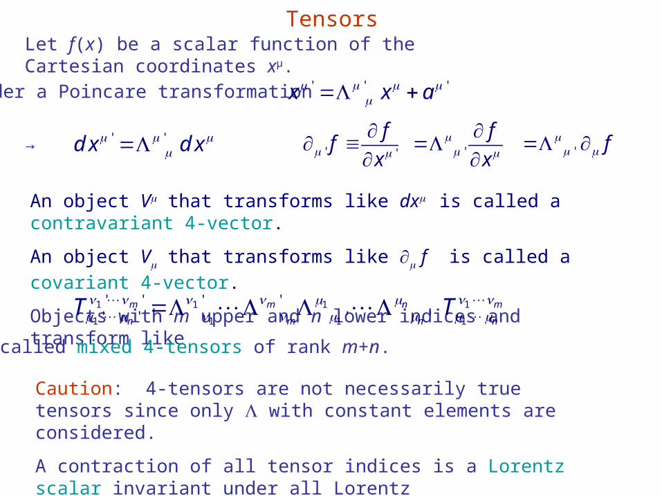
Let f(x) be a scalar function of the Cartesian coordinates xμ.

Under a Poincare transformation ' ' 'x x a

→ ' 'd x d x ' '

ff

x

'

f

x

' f

An object V that transforms like dx is called a contravariant 4-vector.

An object V that transforms like f is called a covariant 4-vector.

Objects with m upper and n lower indices and transform like

1 11 1

1 1 1 1

' ' ''' ' ' '

m m n m

n m n nT T

are called mixed 4-tensors of rank m+n.

Caution: 4-tensors are not necessarily true tensors since only with constant elements are considered.

A contraction of all tensor indices is a Lorentz scalar invariant under all Lorentz transformations. E.g., ημν U μV ν

Lagrangian of a Free Particle

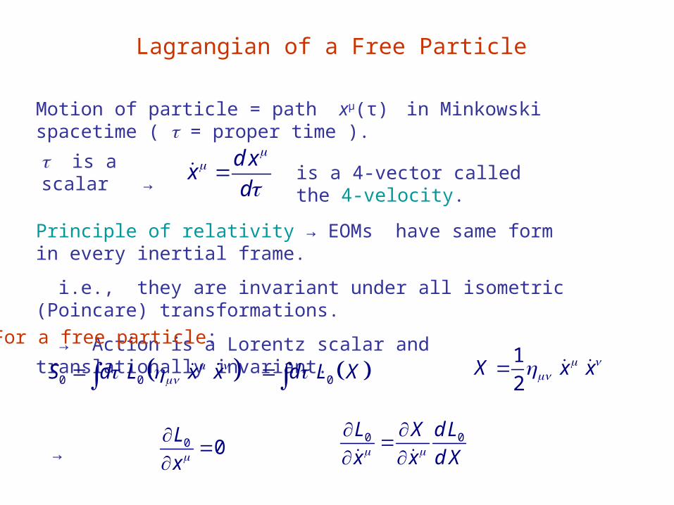
Motion of particle = path xμ(τ) in Minkowski spacetime ( = proper time ).

is a scalar →d x

xd

is a 4-vector called the 4-velocity.

Principle of relativity → EOMs have same form in every inertial frame.

i.e., they are invariant under all isometric (Poincare) transformations.

→ Action is a Lorentz scalar and translationally invariant.

0 0S d L x x 0d L X

For a free particle:1

2X x x

→0 0

L

x

0 0L X d L

x x d X

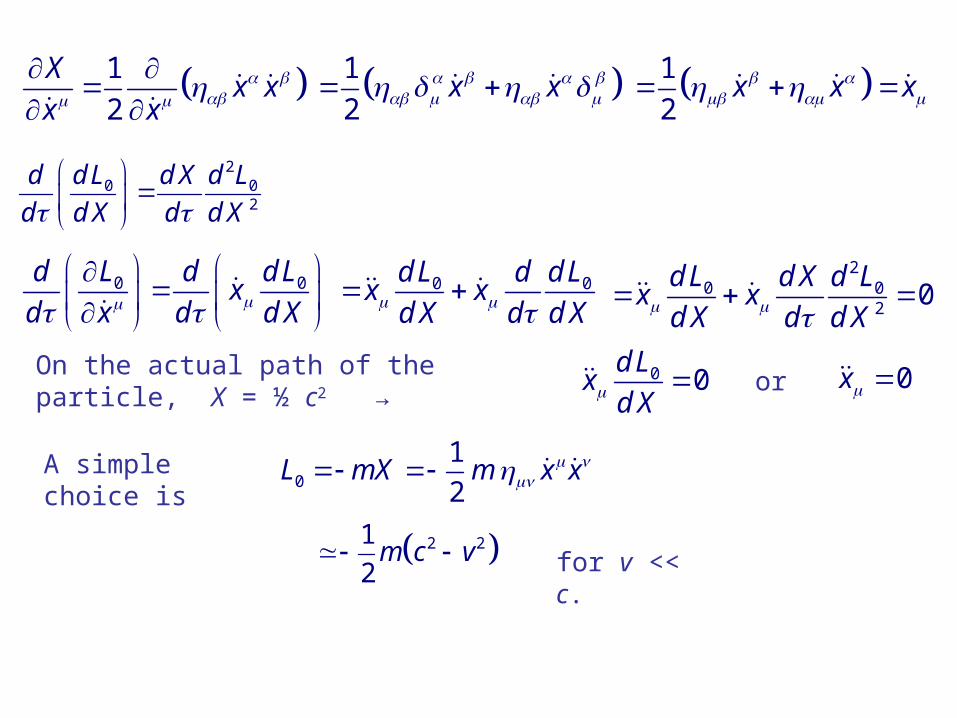
1

2

Xx x

x x

1

2x x

1

2x x x

20 0

2

d d L d X d L

d d X d d X

0 0d L d d Lx

d x d d X

0 0d L d d L

x xd X d d X

2

0 02

0d L d X d L

x xd X d d X

On the actual path of the particle, X = ½ c2 → 0 0d L

xd X or 0x

A simple choice is0

1

2L mX m x x

2 21

2m c v for v << c.

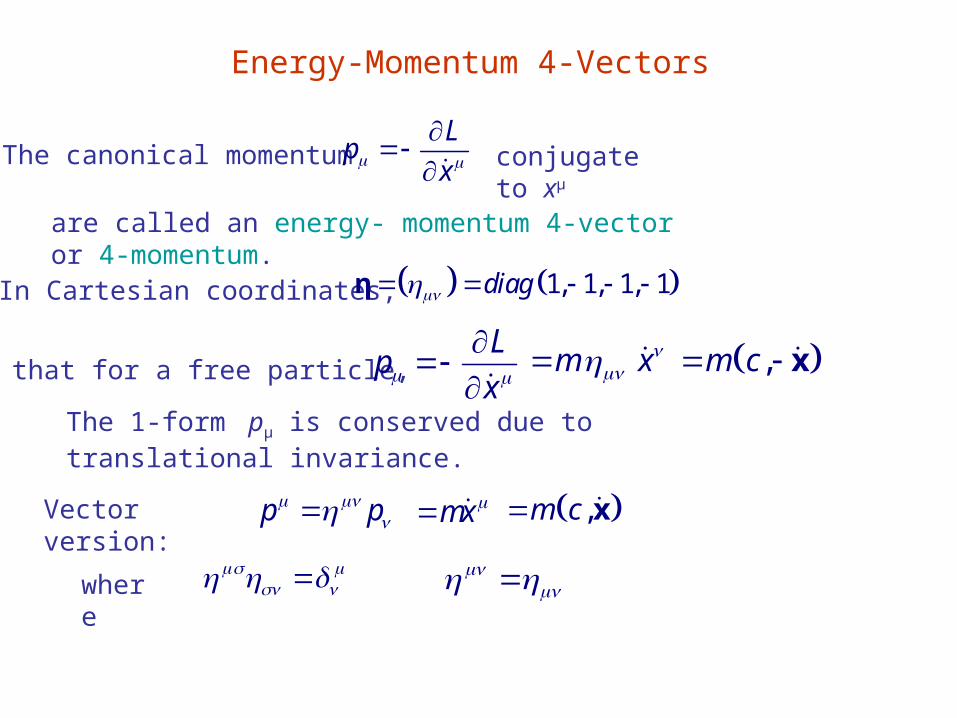
Energy-Momentum 4-Vectors

The canonical momentum L

px

conjugate to xμ

are called an energy- momentum 4-vector or 4-momentum.

In Cartesian coordinates, 1, 1, 1, 1diag η

so that for a free particle, L

px

m x

,m c x

The 1-form pμ is conserved due to translational invariance.

p p mx ,m c x

Vector version:

where

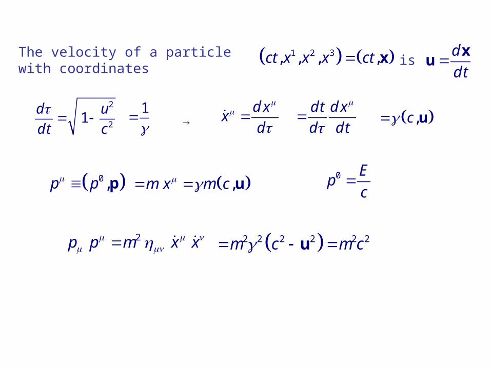
The velocity of a particle with coordinates 1 2 3, , , ,ct x x x ct x is d

d t

xu

2

21

d u

d t c

1

→d x

xd

d t d x

d d t

,c u

0 ,p p p ,m x m c u

0 Ep

c

2p p m x x 2 2 2 2 2 2m c m c u

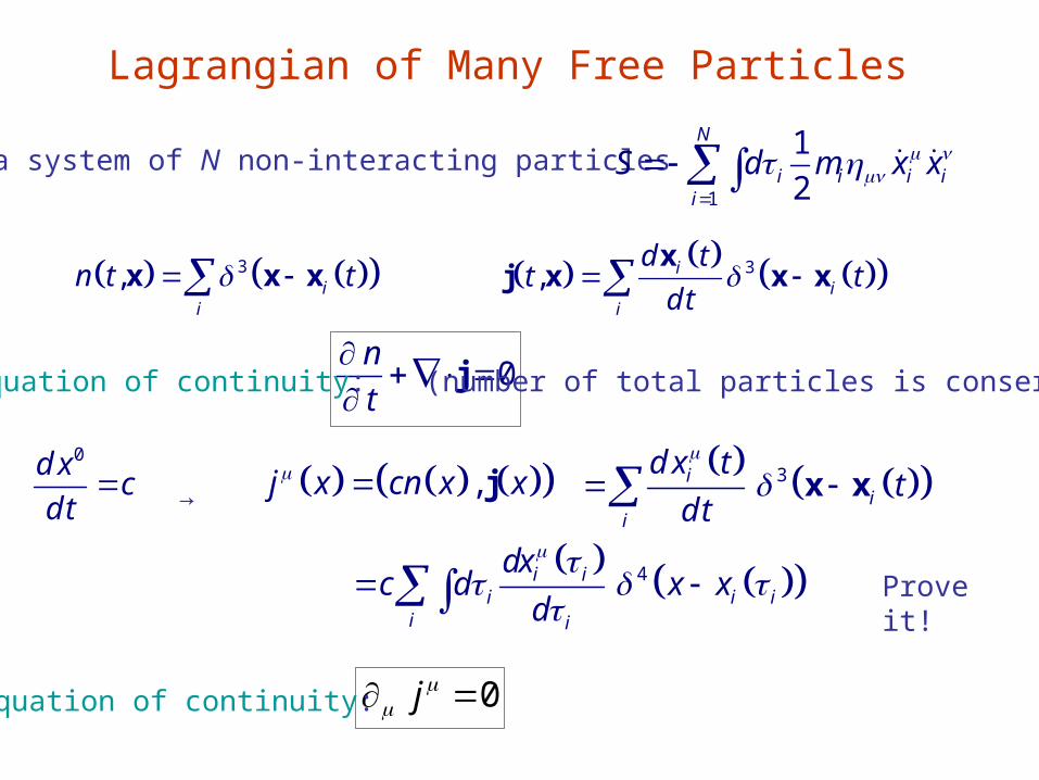
Lagrangian of Many Free Particles

For a system of N non-interacting particles 1

1

2

N

i i i ii

S d m x x

3, ii

n t t x x x 3, ii

i

d tt t

d t x

j x x x

0n

t

jEquation of continuity: (number of total particles is conserved )

0d xc

d t → ,j x cn x x j

3ii

i

d x tt

d t

x x

4i ii i i

i i

dxc d x x

d

Prove it!

0j Equation of continuity:

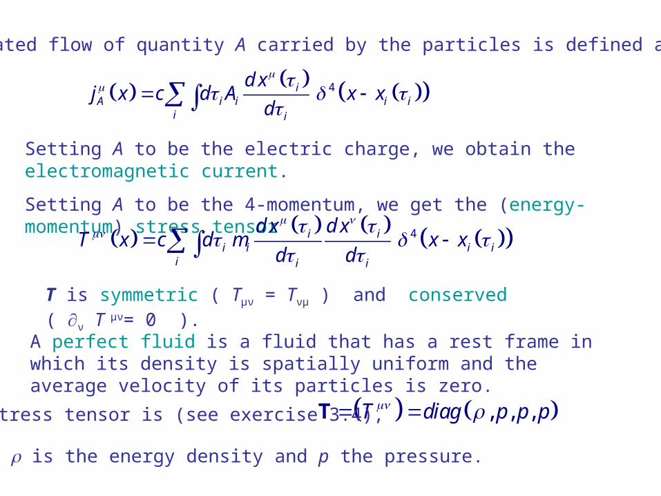
The associated flow of quantity A carried by the particles is defined as

4iA i i i i

i i

d xj x c d A x x

d

Setting A to be the electric charge, we obtain the electromagnetic current.

Setting A to be the 4-momentum, we get the (energy-momentum) stress tensor

4i ii i i i

i i i

d x d xT x c d m x x

d d

T is symmetric ( Tμν = Tνμ ) and conserved ( ν T μν= 0 ).

A perfect fluid is a fluid that has a rest frame in which its density is spatially uniform and the average velocity of its particles is zero.

, , ,T diag p p p TIts stress tensor is (see exercise 3.4),

where is the energy density and p the pressure.

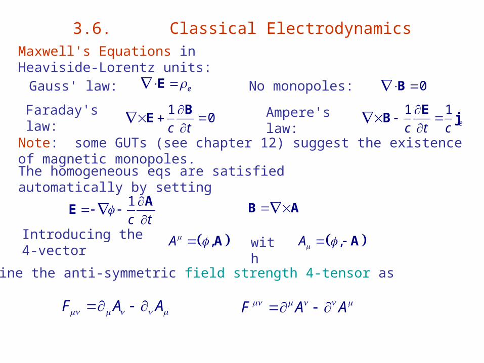
3.6. Classical Electrodynamics

Maxwell's Equations in Heaviside-Lorentz units:

Gauss' law: e E No monopoles: 0 B

Faraday's law: Ampere's law: 1

0c t

B

E1 1

ec t c

E

B j

Note: some GUTs (see chapter 12) suggest the existence of magnetic monopoles.

The homogeneous eqs are satisfied automatically by setting

1

c t

A

E B A

Introducing the 4-vector ,A A ,A A

we define the anti-symmetric field strength 4-tensor as

with

F A A F A A

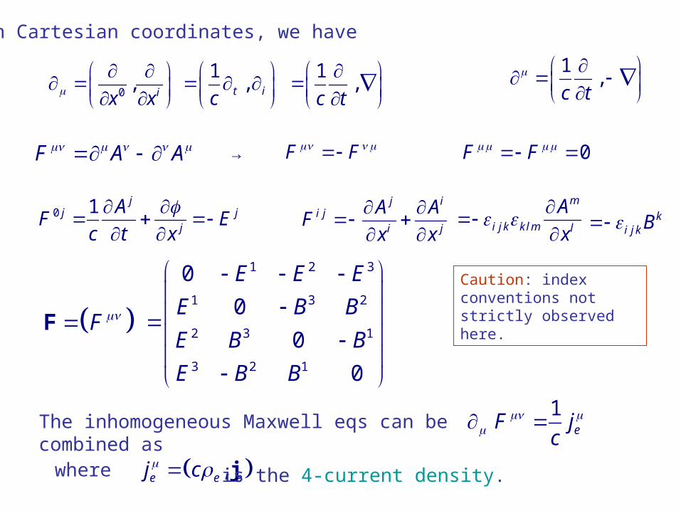
In Cartesian coordinates, we have

0,

ix x

1,t ic

1,

c t

1,

c t

F F 0F F

0 1 jj j

j

AF E

c t x

j ii j

i j

A AF

x x

m

i j k k l m l

A

x

F A A →

F F

1 2 3

1 3 2

2 3 1

3 2 1

0

0

0

0

E E E

E B B

E B B

E B B

The inhomogeneous Maxwell eqs can be combined as1

eF jc

where ,e e ej c j is the 4-current density.

ki j k B

Caution: index conventions not strictly observed here.

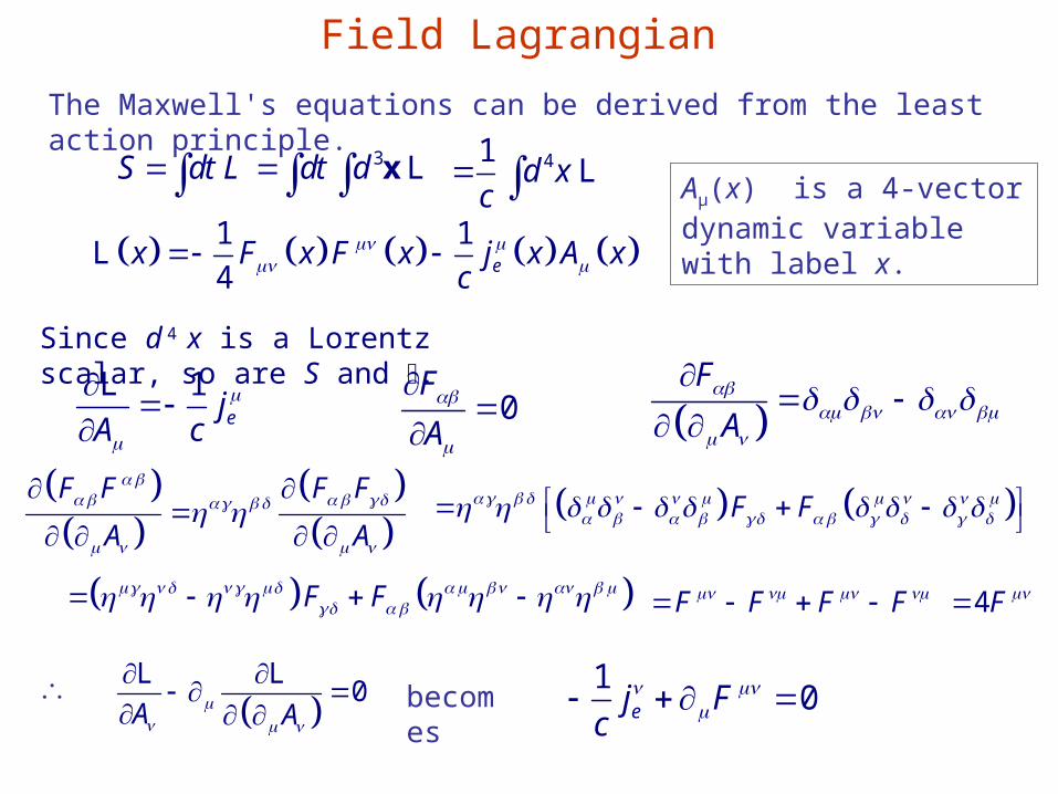
Field Lagrangian

The Maxwell's equations can be derived from the least action principle.

S dt L 3dt d x L 41d x

c L

1 1

4 ex F x F x j x A xc

L

Aμ(x) is a 4-vector dynamic variable with label x.

Since d 4 x is a Lorentz scalar, so are S and .

1ejA c

L

0F

A

F

A

F F F F

A A

F F

F F F F F F 4F

0A A

L L

becomes 10ej F

c

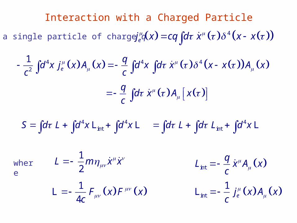
Interaction with a Charged Particle

For a single particle of charge q 4ej x cq d x x x

4 4 42

1e

qd x j x A x d x d x x x A x

c c

qd x A x

c

4 4intS d L d x d x L L 4

intd L d L d x L

1

2L m x x

int

qL x A x

c

1

4F x F x

c

L int

1ej x A x

c

L

where

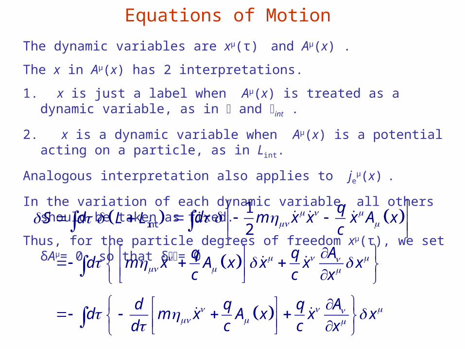
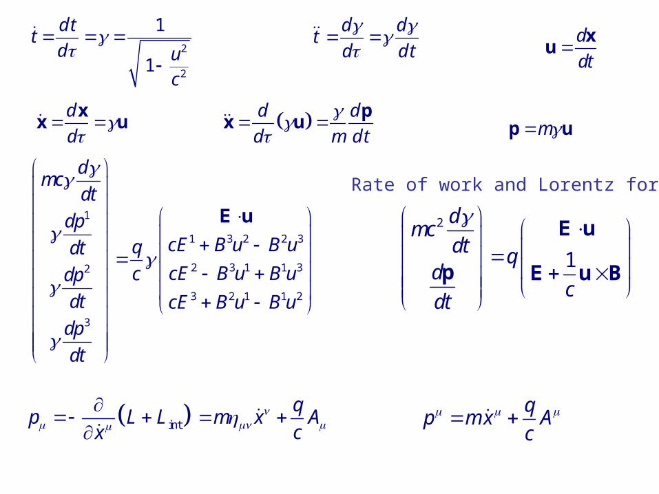
Equations of Motion

The dynamic variables are xμ(τ) and Aμ(x) .

The x in Aμ(x) has 2 interpretations.

1. x is just a label when Aμ(x) is treated as a dynamic variable, as in and int .

2. x is a dynamic variable when Aμ(x) is a potential acting on a particle, as in Lint.

Analogous interpretation also applies to jeμ(x) .

In the variation of each dynamic variable, all others should be taken as fixed.

Thus, for the particle degrees of freedom xμ(τ), we set δAμ= 0 so that δ= 0 intS d L L 1

2

qd m x x x A x

c

q q Ad m x A x x x x

c c x

d q q Ad m x A x x x

d c c x

0q q A

m x A xc c x

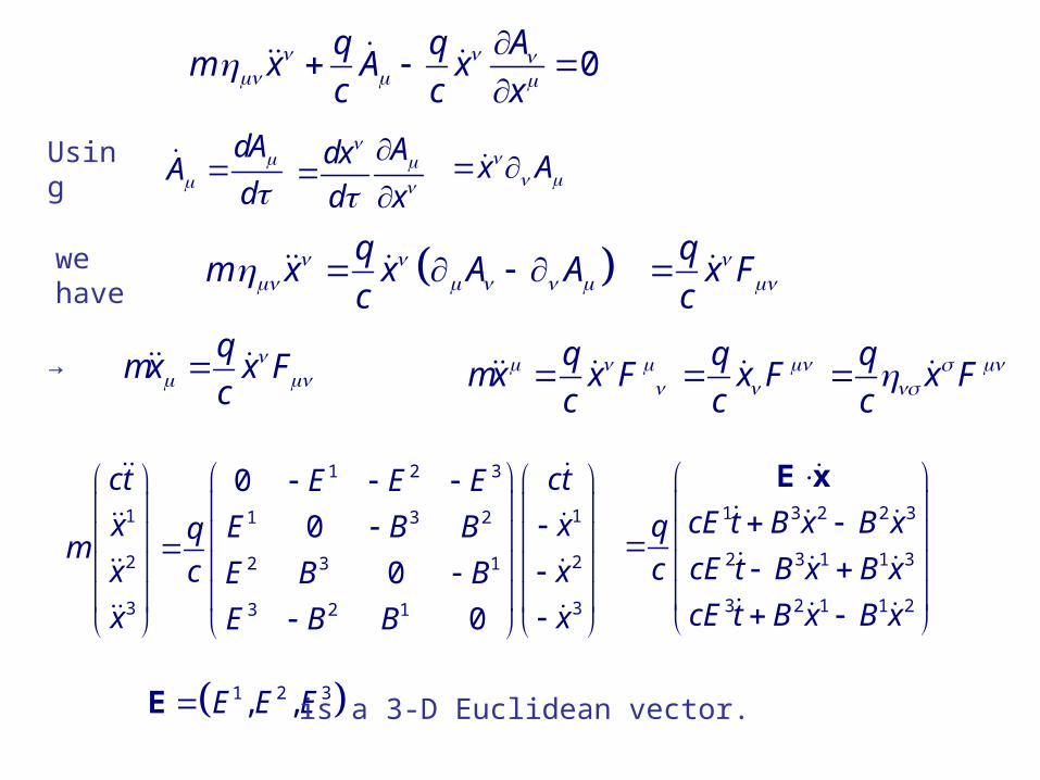
Using dAA

d

Adx

d x

x A

we have qm x x A A

c

qx F

c

qmx x F

c

qmx x F

c

qx F

c

qx F

c

→

1 2 3

1 11 3 2

2 22 3 1

3 33 2 1

0

0

0

0

ct ctE E E

x xE B Bqm

cx xE B B

x xE B B

1 3 2 2 3

2 3 1 1 3

3 2 1 1 2

cE t B x B xq

cE t B x B xc

cE t B x B x

E x

1 2 3, ,E E EE is a 3-D Euclidean vector.

2

2

1

1

d tt

d uc

d dt

d d t

d

dt

xu

d

d

xx u d d

d m dt

p

x u mp u

1

1 3 2 2 3

2 3 1 1 32

3 2 1 1 2

3

dmc

dt

dpcE B u B uqdtcE B u B ucdp

dt cE B u B udp

dt

E u 2

1

dmc

dt qd

cdt

E u

p E u B

Rate of work and Lorentz force

intp L Lx

q

m x Ac

qp m x A

c

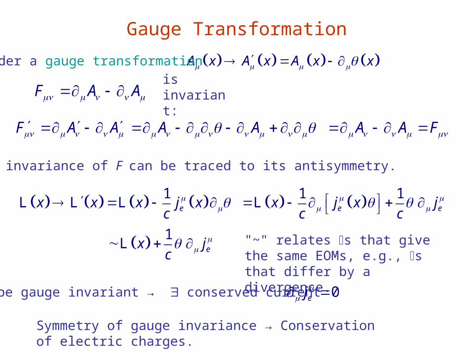
Gauge Transformation

A x A x A x x

F A A

Under a gauge transformation

is invariant:

F A A A A A A F

Gauge invariance of F can be traced to its antisymmetry.

1ex x x j x

c

L L L 1 1e ex j x j

c c

L

1ex j

c

L

"~" relates s that give the same EOMs, e.g., s that differ by a divergence.

be gauge invariant → conserved current 0ej

Symmetry of gauge invariance → Conservation of electric charges.

3.7. Geometry in Classical Physics

3.7.1. More on Tensors

3.7.2. Differential Forms, Dual Tensors and Maxwell's Equations

3.7.3. Configuration Space and Its Relatives

3.7.4. The Symplectic Geometry of Phase Space

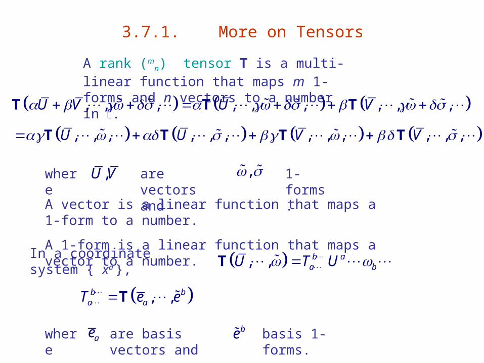
3.7.1. More on Tensors

A rank (mn) tensor T is a multi-linear function that

maps m 1-forms and n vectors to a number in .

, , , , , , , , ,U V U V T T T

, , , , , , , , , , , ,U U V V T T T T

A vector is a linear function that maps a 1-form to a number.

A 1-form is a linear function that maps a vector to a number.

In a coordinate system { xa }, , , b aa bU T U T

, ,b ba aT e eT

where ,U V are vectors and , 1-forms.

where ae are basis vectors and be basis 1-forms.

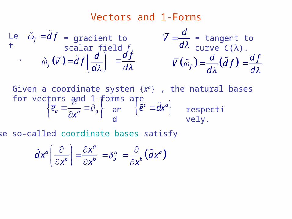
Vectors and 1-Forms

Letf d f d

Vd

= gradient to scalar field f. = tangent to curve C(λ).

→ f

dV d f

d

d f

d

f

dV d f

d

d f

d

Given a coordinate system {xa} , the natural bases for vectors and 1-forms are

a aae

x

a ae dx and respectively.

These so-called coordinate bases satisfy

aa

b b

xd x

x x

ab a

bd x

x

aaV V e a

aV

x

a

a e aa d x

a ba b

V d x Vx

b aa bV d x

x

b a a

a b aV V

a bba

V V d xx

a b

b aV d x

x

a b ab a aV V

V V

Under a coordinate transformation, 'a ax x

'a ad x d x'a

aa

xd x

x

'a a

a d x 'a ax x

'

a

a a

x

x x

'a

a ax

''

' '

a ba b

a a a a

x x

x x

bbaa

x

x

''

aa d x '

'a a b

a a b d x a ba b d x a

a d x

→

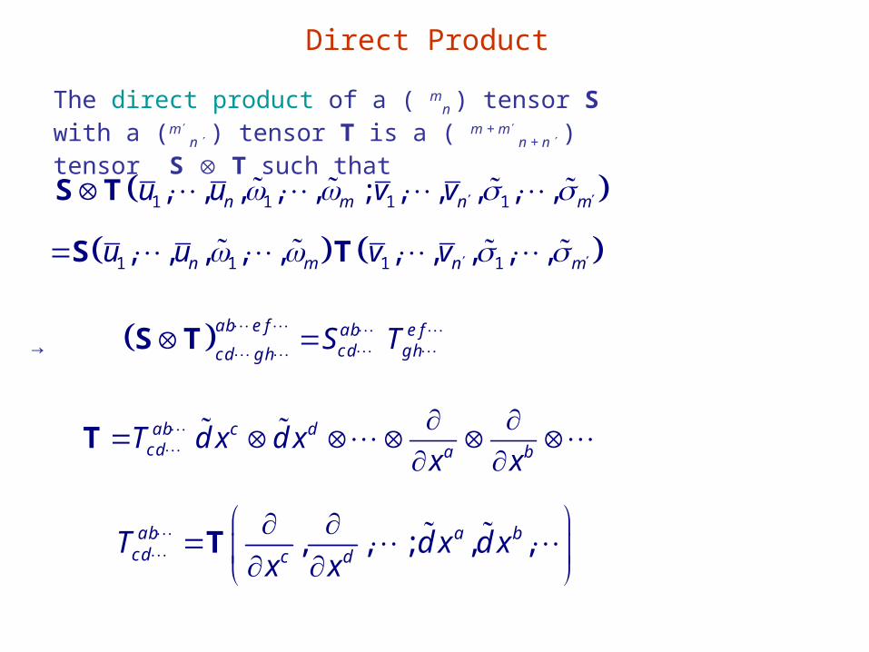
Direct Product

The direct product of a ( mn ) tensor S with a (m

n ) tensor T is a ( m + m

n + n ) tensor S T such that

1 1 1 1, , , , , ; , , , , ,n m n mu u v v S T

1 1 1 1, , , , , , , , , ,n m n mu u v v S T

ab e f ab e f

cd g hcd g hS T S T

→

ab c dcd a b

T d x d xx x

T

, , ; , ,ab a bcd c d

T d x d xx x

T

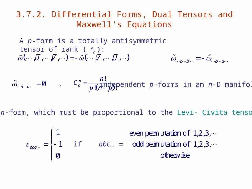
3.7.2. Differential Forms, Dual Tensors and Maxwell's Equations

A p-form is a totally antisymmetric tensor of rank ( 0p ):

, , , , , , , ,U V V U a b b a

0a a → !

! !np

nC

p n p

independent p-forms in an n-D manifold.

only one n-form, which must be proportional to the Levi- Civita tensor density

1

1

0abc

even permutation of 1,2,3,

odd permutation of 1,2,3,

otherwise

if abc…

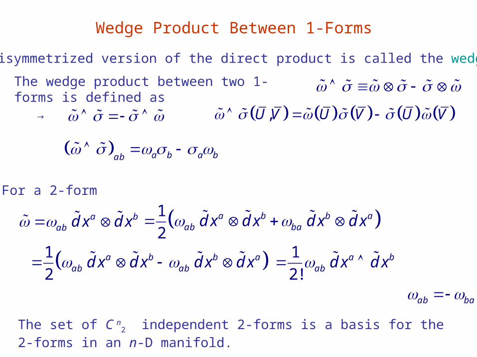
Wedge Product Between 1-Forms

A totally antisymmetrized version of the direct product is called the wedge product .

The wedge product between two 1-forms is defined as

→ ,U V U V U V

a b a bab

For a 2-form

a bab d x d x 1

2a b b a

ab bad x d x d x d x

1

2a b b a

ab abd x d x d x d x

ab ba

1

2!a b

ab d x d x

The set of C n2 independent 2-forms is a basis for the 2-forms in an n-D manifold.

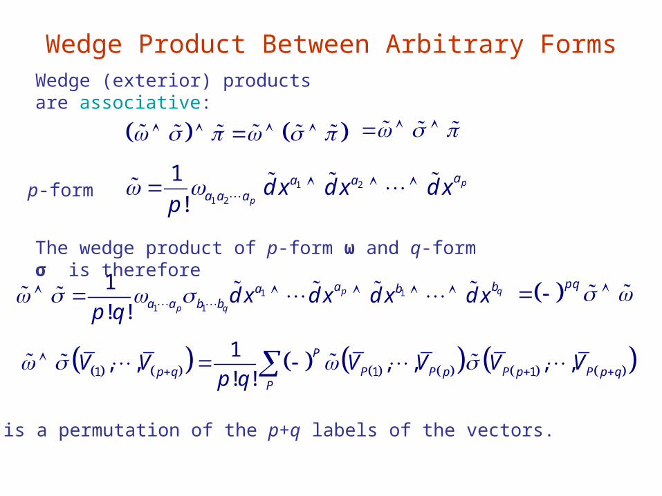
Wedge Product Between Arbitrary Forms

Wedge (exterior) products are associative:

1 2

1 2

1

!p

p

aa aa a a d x d x d x

p

p -form

The wedge product of p-form ω and q-form σ is therefore

1 1

1 1

1

! !p q

p q

a ba ba a b b d x d x d x d x

p q

pq

1 1 1

1, , , , , ,

! !P

p q P P p P p P p qP

V V V V V Vp q

where P is a permutation of the p+q labels of the vectors.

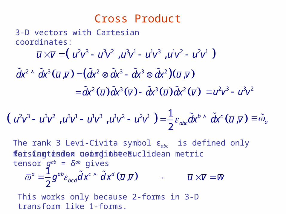
Cross Product

2 3 3 2 3 1 1 3 1 2 2 1, ,u v u v u v u v u v u v u v

3-D vectors with Cartesian coordinates:

2 3 2 3 3 2, ,dx dx u v dx dx dx dx u v

2 3 3 2dx u dx v dx u dx v 2 3 3 2u v u v

2 3 3 2 3 1 1 3 1 2 2 1 1, , ,

2b c

abcu v u v u v u v u v u v dx dx u v a

The rank 3 Levi-Civita symbol εabc is defined only for Cartesian coordinates.

Raising index using the Euclidean metric tensor gab = δab gives

1,

2a ab c d

bcdg d x d x u v → u v w

This works only because 2-forms in 3-D transform like 1-forms.

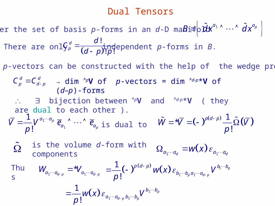
Dual Tensors

Consider the set of basis p-forms in an d-D manifold 1 pa aB d x d x

There are only !

! !dp

dC

d p p

independent p-forms in B.

Similarly, p-vectors can be constructed with the help of the wedge product.

d dp d pC C → dim pV of p-vectors = dim d-p*V of (d–p)-forms

bijection between pV and d-p*V ( they are dual to each other ).

1

1

1

!p

p

a a

a aV V e ep

is dual to 1*

!p d p

W V Vp

1 1d da a a aw x is the volume d-form with components

Thus1 1

*d p d pa a a aW V

1

1 1

1

!p

d p p

b b

a a b bw x Vp

1

1 1

1

!p

p d p

p d p b b

b b a aw x Vp

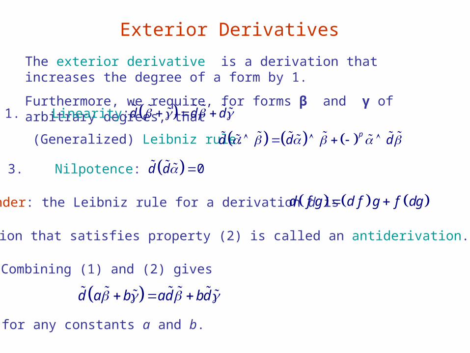
Exterior Derivatives

The exterior derivative is a derivation that increases the degree of a form by 1.

Furthermore, we require, for forms β and γ of arbitrary degrees, that

1. Linearity: d d d

2. (Generalized) Leibniz rule:

3. Nilpotence:

pd d d

0d d

A derivation that satisfies property (2) is called an antiderivation.

Reminder: the Leibniz rule for a derivation d is d f g d f g f dg

Combining (1) and (2) gives

d a b ad bd

for any constants a and b.

p-forms

Taking a scalar function f as a 0-form, we have a 1-form aa

fd f d x

x

Consistency check: 1

1 aa

xd x d x

x

1 1aa d x d x

Note that ad x is a 1-form while the ordinary derivative dxa is a 1-vector.

Also, most authors (Lawrie is one) use the symbol d to denote d

aa dx

aad d dx 0a a

a ad dx d dx b aab

dx dxx

0ad dx

a bab

dx dxx

,a b

a b dx dx ,

b ab a dx dx

,a b

b a dx dx , ,

1

2a b

a b b a dx dx

, ,a b b aabd

For a 1-form

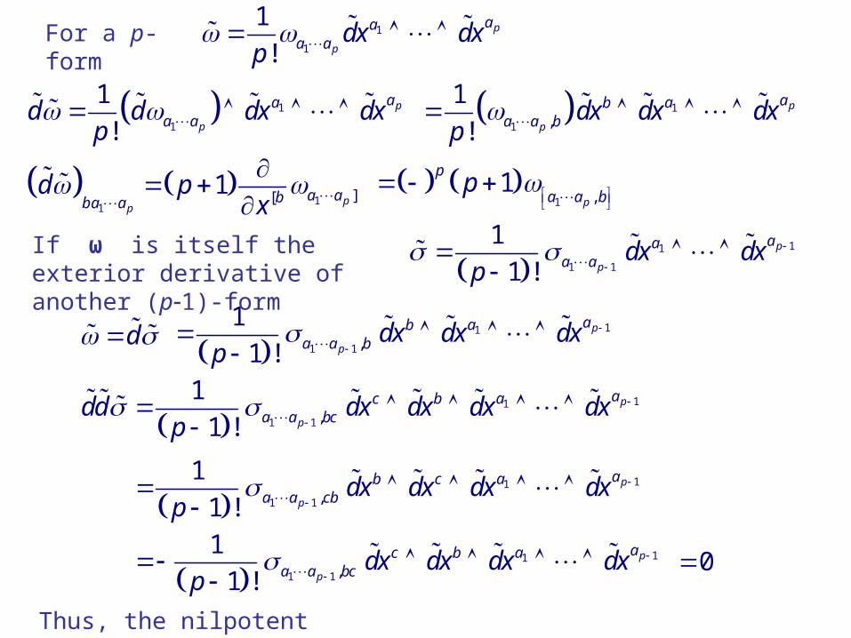
For a p-form 1

1

1

!p

p

aaa a dx dx

p

1

1

1

!p

p

aaa ad d dx dx

p 1

1 ,

1

!p

p

aaba a b dx dx dx

p

1

1][

1p

pa abba a

d px

1 ,1

p

p

a a bp

11

1 1

1

1 !p

p

aaa a dx dx

p

d 11

1 1 ,

1

1 !p

p

aaba a b dx dx dx

p

11

1 1 ,

1

1 !p

p

aac ba a bcdd dx dx dx dx

p

11

1 1 ,

1

1 !p

p

aab ca a cb dx dx dx dx

p

0

If ω is itself the exterior derivative of another (p1)-form

11

1 1 ,

1

1 !p

p

aac ba a bc dx dx dx dx

p

Thus, the nilpotent assumption is consistent.

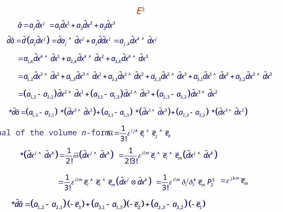
E3 j

ja a dx 1 2 31 2 3a dx a dx a dx

jjda d a dx j j

j jda dx a ddx ,

k jj ka dx dx

1 2 31, 2, 3,

k k kk k ka dx dx a dx dx a dx dx

2 1 3 1 1 2 1 3 1 3 2 31, 2 1, 3 2,1 2, 3 3,1 3, 2a dx dx a dx dx a dx dx a dx dx a dx dx a dx dx

2 1 1 3 3 21, 2 2,1 3,1 1, 3 2, 3 3, 2a a dx dx a a dx dx a a dx dx

2 1 1 3 3 21, 2 2,1 3,1 1, 3 2, 3 3, 2* * * *da a a dx dx a a dx dx a a dx dx

1

3!i j k

i j ke e e Dual of the volume n-form:

1*

2!j k j kdx dx dx dx 1

2!3!il m j k

i l me e e dx dx

1

3!il m j k

i l me e e dx dx 32

1

3!il m j k

i l me P j k m

me

1, 2 2,1 3 3,1 1, 3 2 2, 3 3, 2 1*da a a e a a e a a e

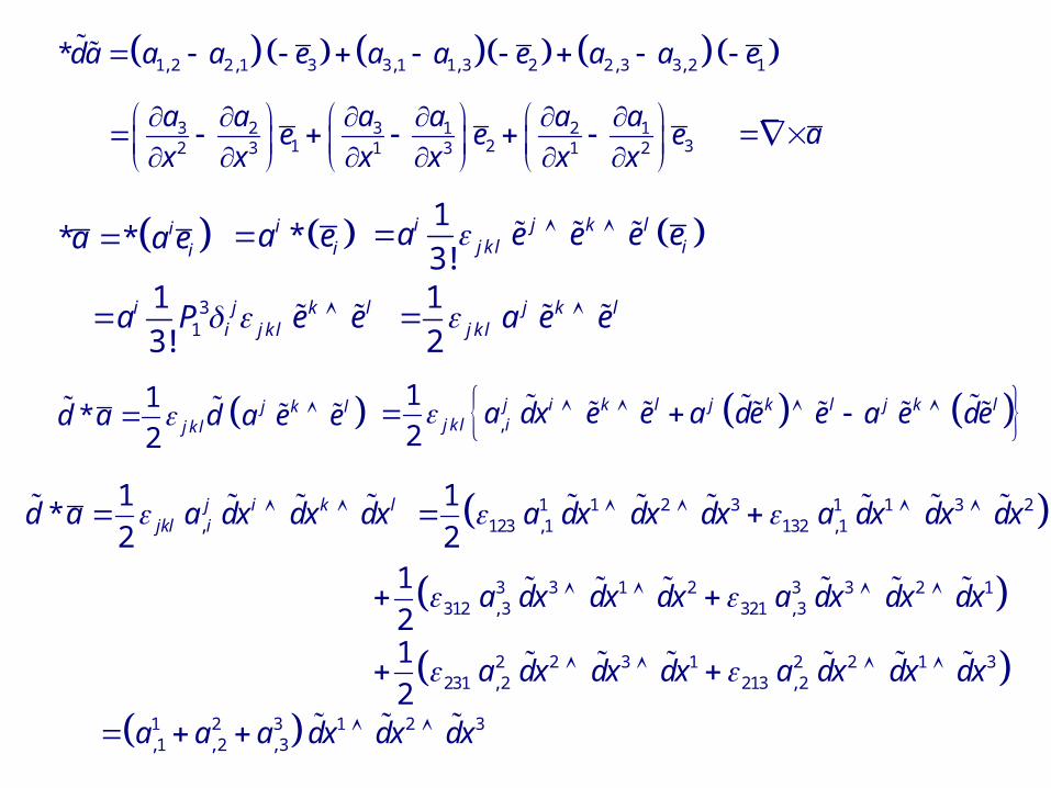
1, 2 2,1 3 3,1 1, 3 2 2, 3 3, 2 1*da a a e a a e a a e

3 2 3 1 2 11 2 32 3 1 3 1 2

a a a a a ae e e

x x x x x x

a

* * iia a e *i

ia e 1

3!i j k l

j k l ia e e e e

31

1

3!i j k l

i j k la P e e 1

2j k l

j k l a e e

1*

2j k l

j k ld a d a e e ,

1

2j i k l j k l j k l

j k l ia dx e e a de e a e de

,

1*

2j i k l

jkl id a a dx dx dx 1 1 2 3 1 1 3 2123 ,1 132 ,1

1

2a dx dx dx a dx dx dx

2 2 3 1 2 2 1 3231 , 2 213 , 2

1

2a dx dx dx a dx dx dx

3 3 1 2 3 3 2 1312 , 3 321 , 3

1

2a dx dx dx a dx dx dx

1 2 3 1 2 3,1 , 2 , 3a a a dx dx dx

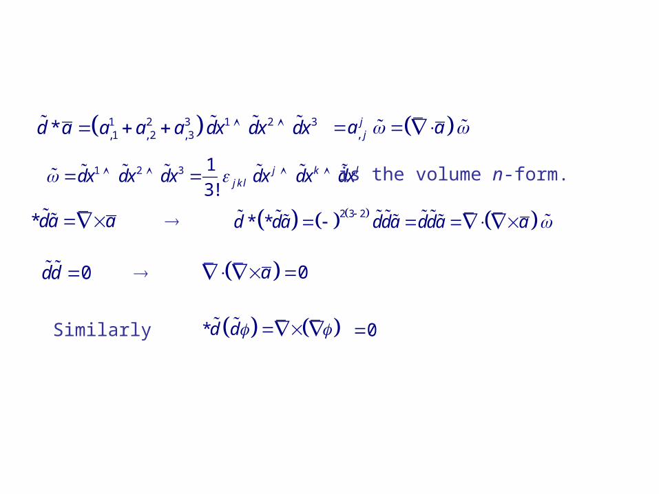
1 2 3 1 2 3,1 , 2 , 3*d a a a a dx dx dx ,

jja a

1 2 3 1

3!j k l

j k ldx dx dx dx dx dx is the volume n-form.

2 3 2* *d da dda dda a

0dd 0a

*da a

*d d 0Similarly

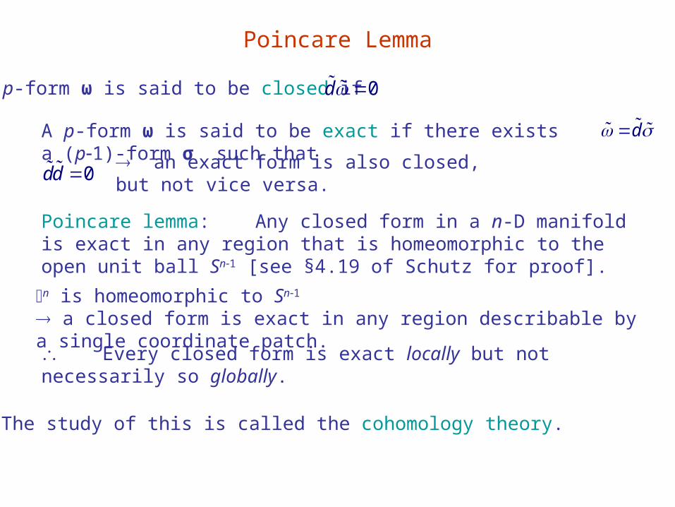
Poincare Lemma

A p-form ω is said to be exact if there exists a (p1)-form σ such that

A p-form ω is said to be closed if 0d

d

0dd an exact form is also closed, but not vice versa.

Poincare lemma: Any closed form in a n-D manifold is exact in any region that is homeomorphic to the open unit ball Sn1 [see §4.19 of Schutz for proof].

n is homeomorphic to Sn1 a closed form is exact in any region describable by a single coordinate patch.

Every closed form is exact locally but not necessarily so globally.

The study of this is called the cohomology theory.

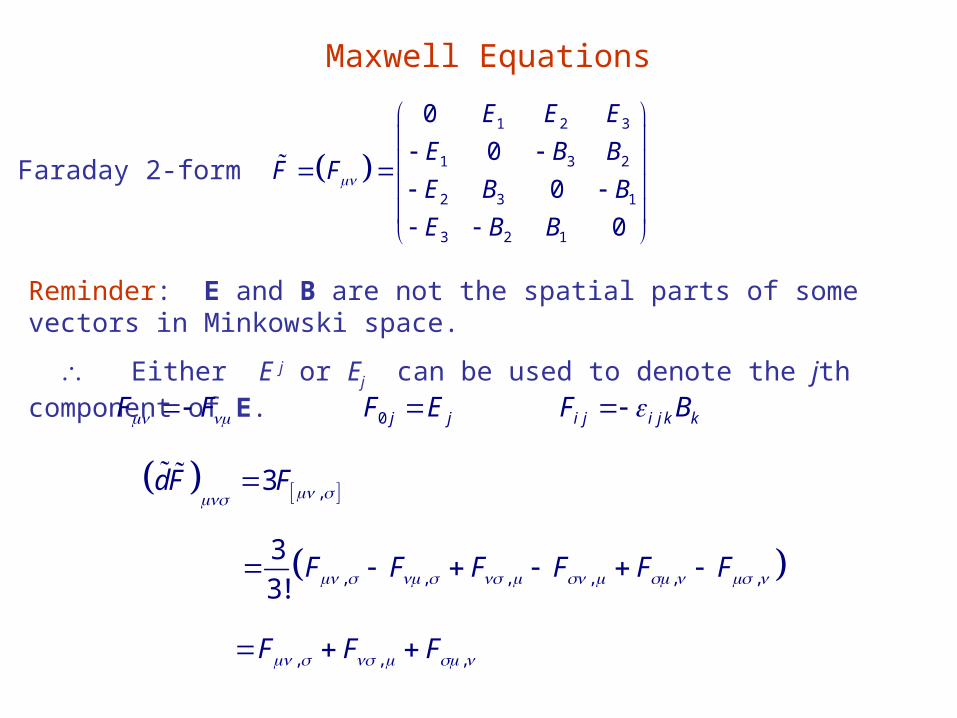
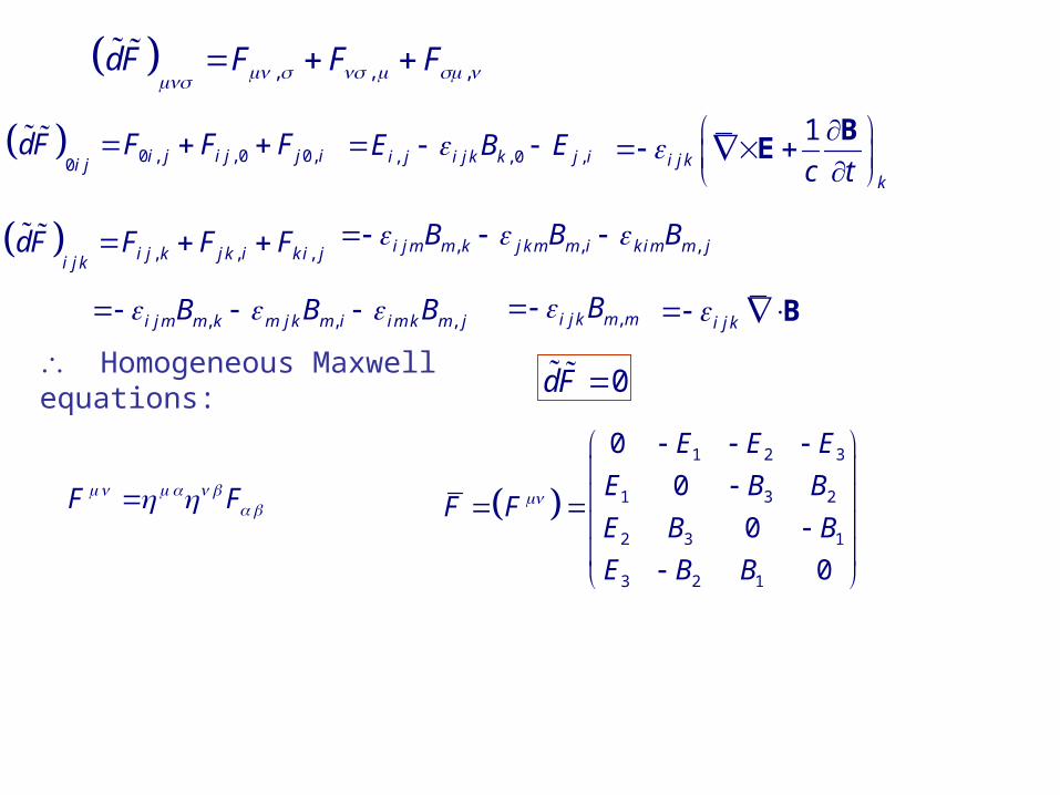
Maxwell Equations

Faraday 2-form 1 2 3

1 3 2

2 3 1

3 2 1

0

0

0

0

E E E

E B BF F

E B B

E B B

Reminder: E and B are not the spatial parts of some vectors in Minkowski space.

Either E j or Ej can be used to denote the jth component of E. F F 0 j jF E i j i j k kF B

,3dF F

, , , , , ,

3

3!F F F F F F

, , ,F F F

, , ,dF F F F

0 , , 0 0,0 i j i j j ii jdF F F F

, , 0 ,i j i j k k j iE B E 1i j k

kc t

BE

, , ,i j k j k i k i ji j kdF F F F , , ,i j m m k j k m m i k im m jB B B

, , ,i j m m k m j k m i im k m jB B B ,i j k m mBi j k B

Homogeneous Maxwell equations: 0dF

F F

1 2 3

1 3 2

2 3 1

3 2 1

0

0

0

0

E E E

E B BF F

E B B

E B B

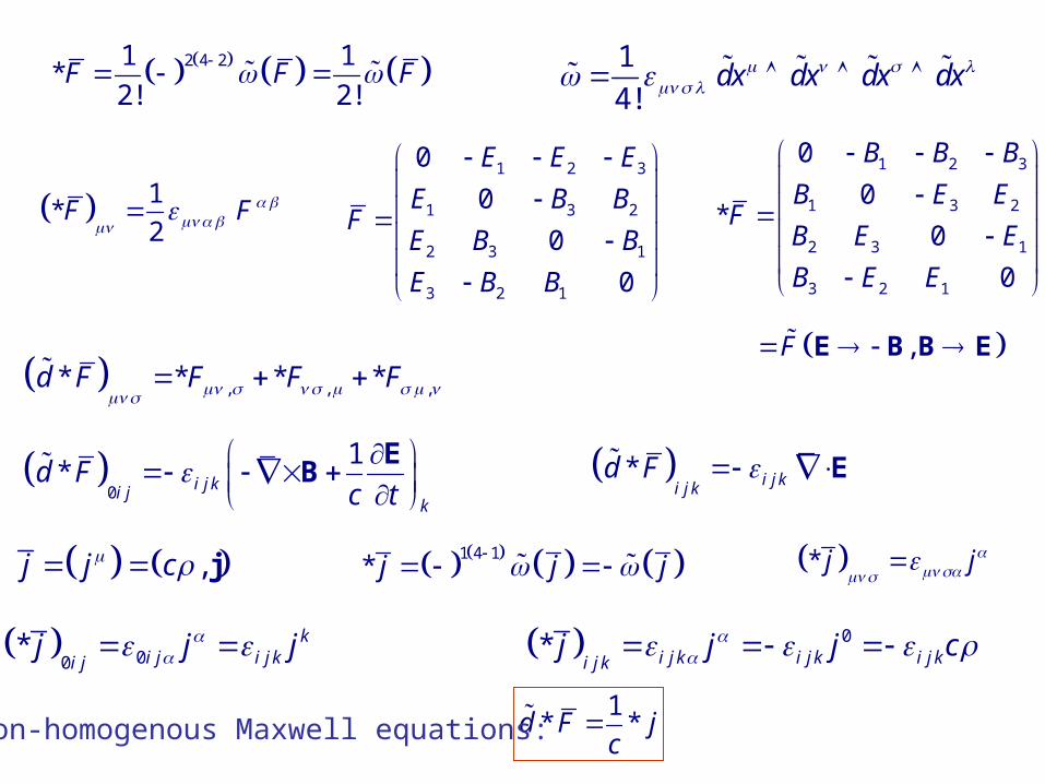
2 4 21 1*

2! 2!F F F 1

4!dx dx dx dx

1*

2F F

1 2 3

1 3 2

2 3 1

3 2 1

0

0*

0

0

B B B

B E EF

B E E

B E E

1 2 3

1 3 2

2 3 1

3 2 1

0

0

0

0

E E E

E B BF

E B B

E B B

,F E B B E

, , ,* * * *d F F F F

0

1* i j ki j

k

d Fc t

E

B * i j ki j kd F E

,j j c j 1 4 1* j j j * j j

00* k

i j i j ki jj j j

0* i j k i j k i j ki j kj j j c

1* *d F j

cNon-homogenous Maxwell equations:

3.7.3. Configuration Space and Its Relatives

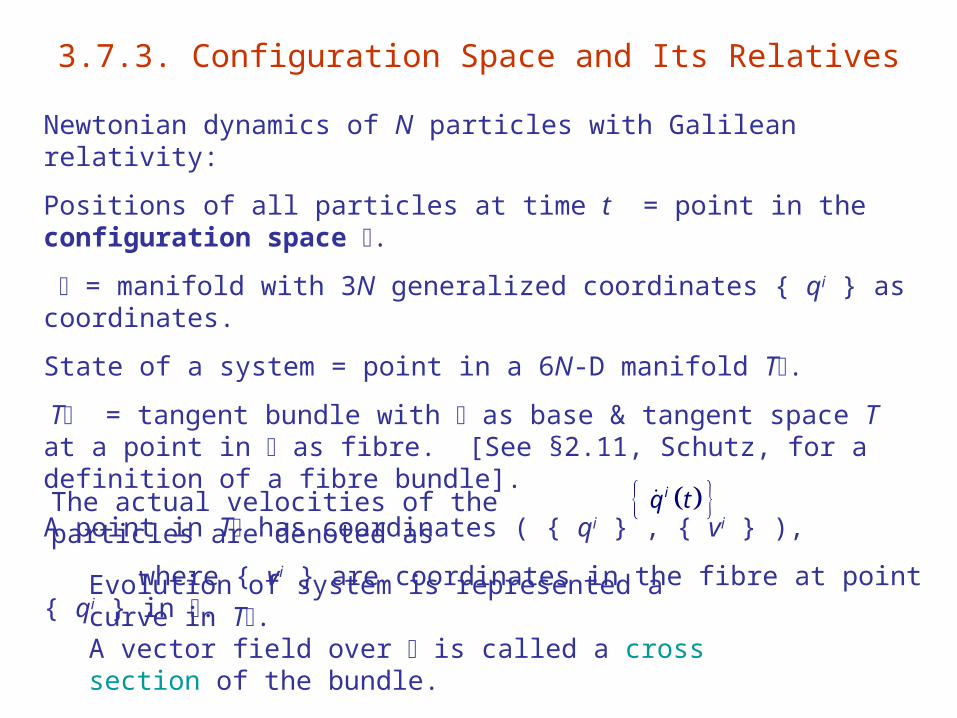
Newtonian dynamics of N particles with Galilean relativity:

Positions of all particles at time t = point in the configuration space .

= manifold with 3N generalized coordinates { qi } as coordinates.

State of a system = point in a 6N-D manifold T.

T = tangent bundle with as base & tangent space T at a point in as fibre. [See §2.11, Schutz, for a definition of a fibre bundle].

A point in T has coordinates ( { qi } , { vi } ),

where { vi } are coordinates in the fibre at point { qi } in .

The actual velocities of the particles are denoted as

Evolution of system is represented a curve in T. A vector field over is called a cross section of the bundle.

iq t

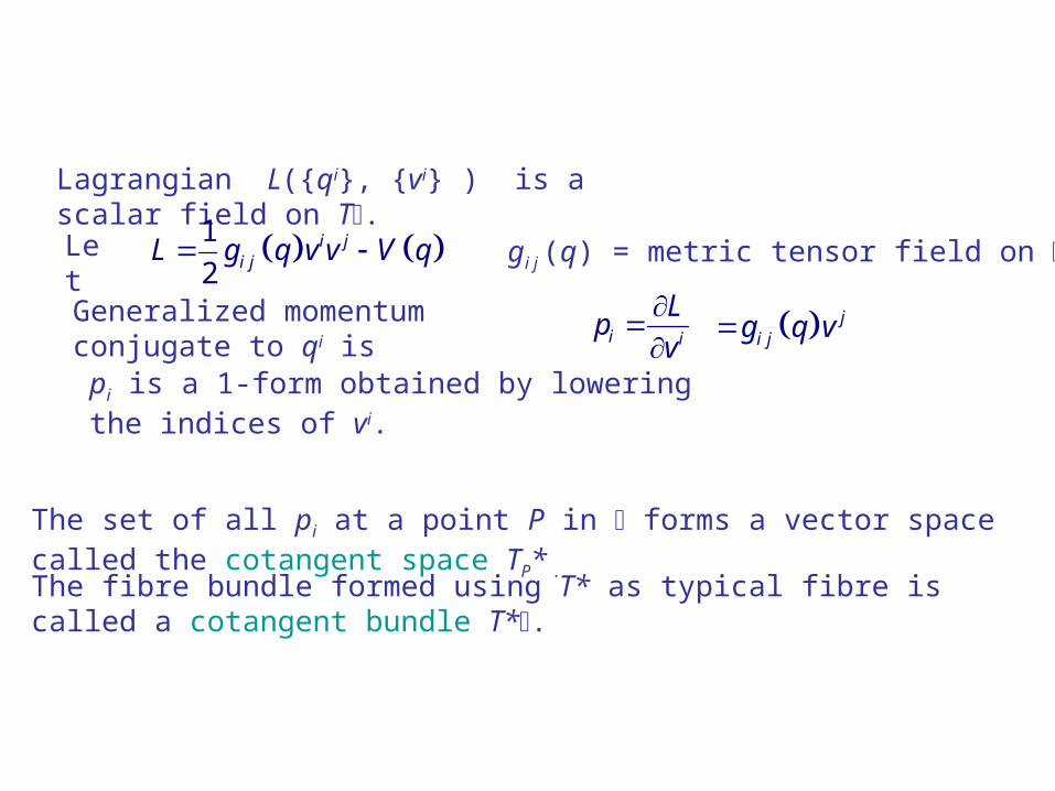
Lagrangian L({qi}, {vi} ) is a scalar field on T.

Let 1

2i j

i jL g q v v V q gi j (q) = metric tensor field on .

Generalized momentum conjugate to qi is i i

Lp

v

ji jg q v

pi is a 1-form obtained by lowering the indices of vi.

The set of all pi at a point P in forms a vector space called the cotangent space TP* .

The fibre bundle formed using T* as typical fibre is called a cotangent bundle T*.

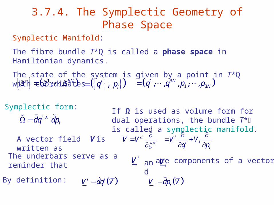
3.7.4. The Symplectic Geometry of Phase Space

Symplectic Manifold:

The fibre bundle T*Q is called a phase space in Hamiltonian dynamics.

The state of the system is given by a point in T*Q with coordinates

1 6, , N ,iiq p 1 3

1 3, , , , ,NNq q p p

Symplectic form:i

idq dp If Ω is used as volume form for dual operations, the bundle T* is called a symplectic manifold.

A vector field V is written as V V

i

iii

V Vq p

The underbars serve as a reminder that iViVand are components of a vector.

By definition: i iV dq V i iV dp V

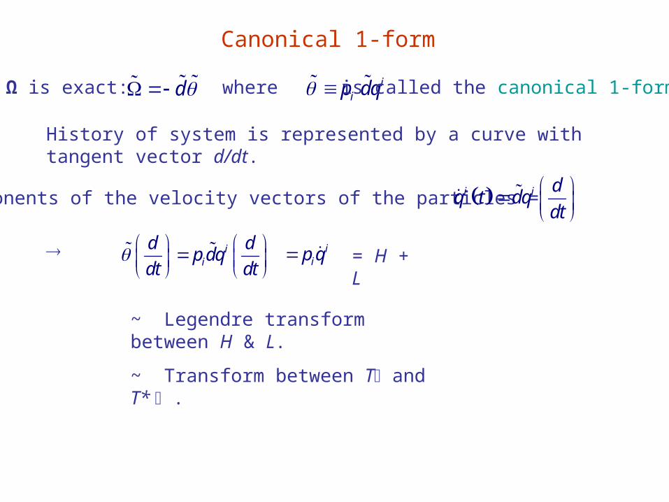
Canonical 1-form

Ω is exact: d iip dq where is called the canonical 1-form.

History of system is represented by a curve with tangent vector d/dt.

Components of the velocity vectors of the particles = i i dq t dq

dt

ii

d dp dq

dt dt

iip q = H + L

~ Legendre transform between H & L.

~ Transform between T and T* .

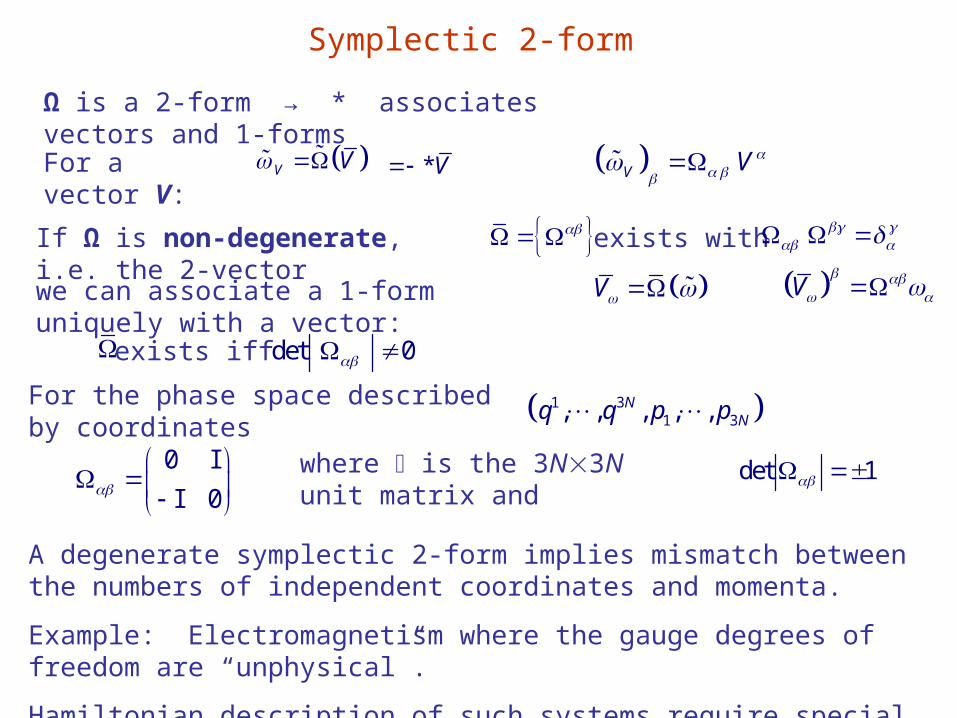
Symplectic 2-form

Ω is a 2-form → * associates vectors and 1-forms

For a vector V: V V *V V V

If Ω is non-degenerate, i.e. the 2-vector exists with

we can associate a 1-form uniquely with a vector: V V

det 0 exists iff

For the phase space described by coordinates 1 31 3, , , , ,N

Nq q p p

0

0

I

Iwhere is the 3N3N unit matrix and

det 1

A degenerate symplectic 2-form implies mismatch between the numbers of independent coordinates and momenta.

Example: Electromagnetism where the gauge degrees of freedom are “unphysical”.

Hamiltonian description of such systems require special techniques.

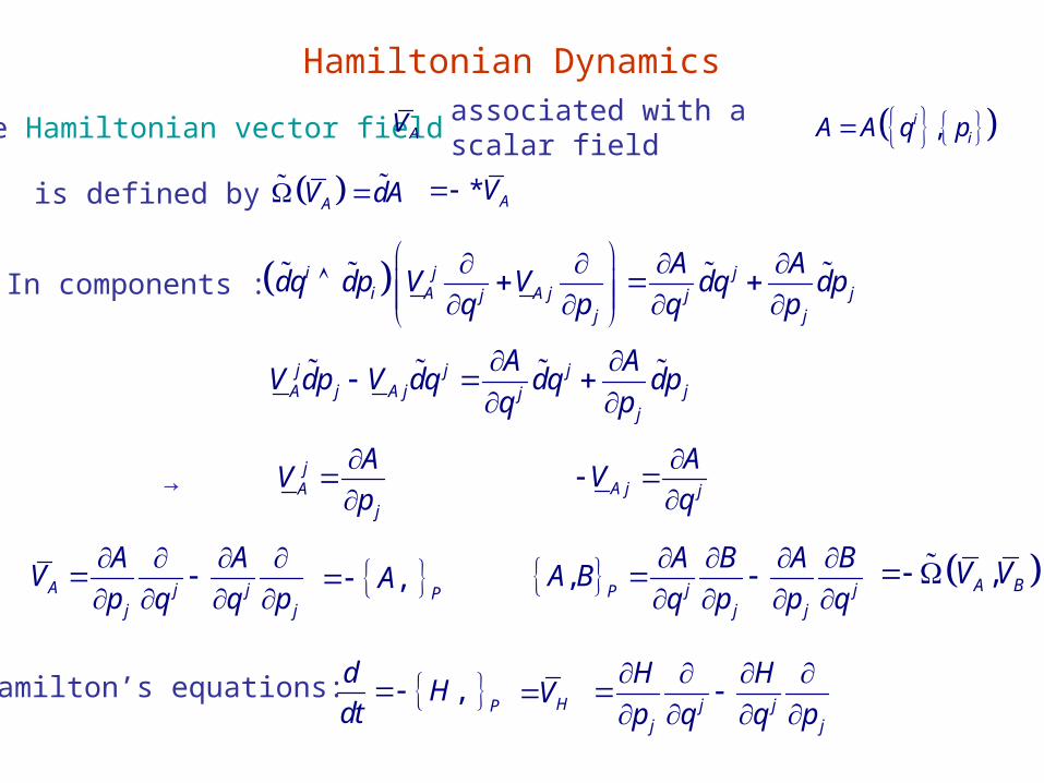
Hamiltonian Dynamics

associated with a scalar field ,iiA A q pThe Hamiltonian vector field AV

is defined by AV dA * AV

In components : i j ji A A j jj j

j j

A Adq dp V V dq dp

q p q p

j j jA j A j jj

j

A AV dp V dq dq dp

q p

→ j

Aj

AV

p

A j j

AV

q

A j jj j

A AV

p q q p

,P

A ,j jP

j j

A B A BA B

q p p q

,A BV V

Hamilton’s equations: HV j j

j j

H H

p q q p

,P

dH

dt

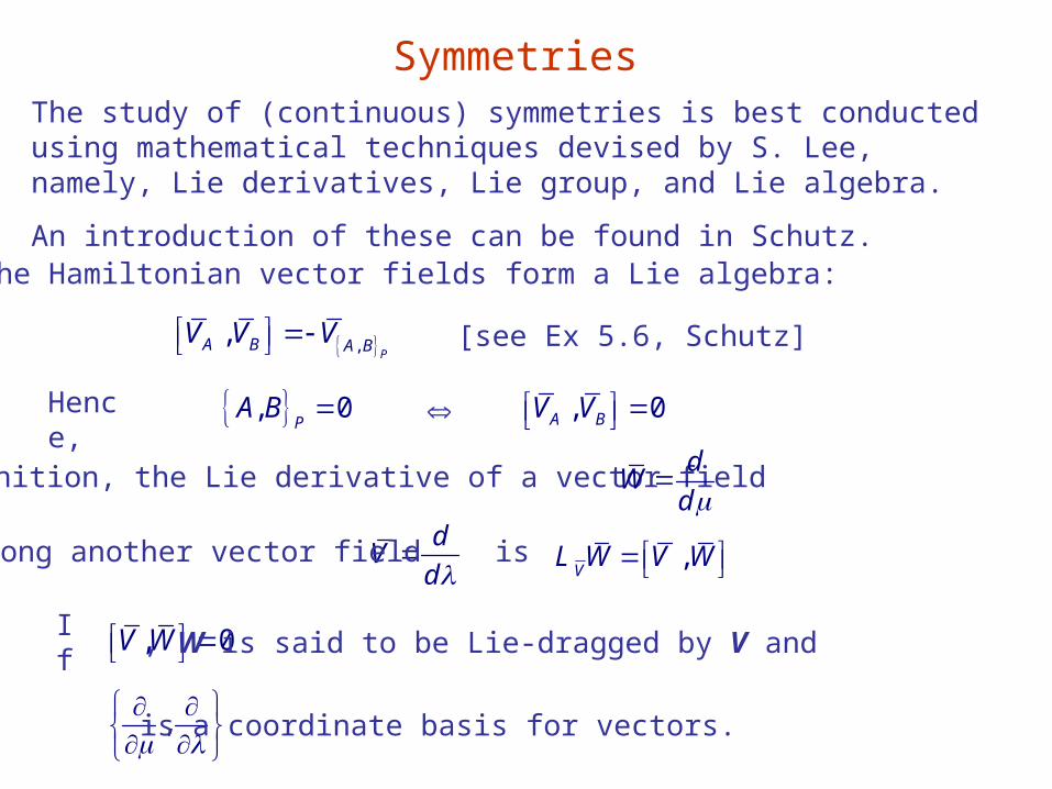
Symmetries The study of (continuous) symmetries is best conducted using mathematical techniques devised by S. Lee, namely, Lie derivatives, Lie group, and Lie algebra.

An introduction of these can be found in Schutz.

,,P

A B A BV V V [see Ex 5.6, Schutz]

First, the Hamiltonian vector fields form a Lie algebra:

Hence, , 0P

A B , 0A BV V

By definition, the Lie derivative of a vector field dW

d

dV

d ,

VW V W Lalong another vector field is

, 0V W

If , W is said to be Lie-dragged by V and

,

is a coordinate basis for vectors.

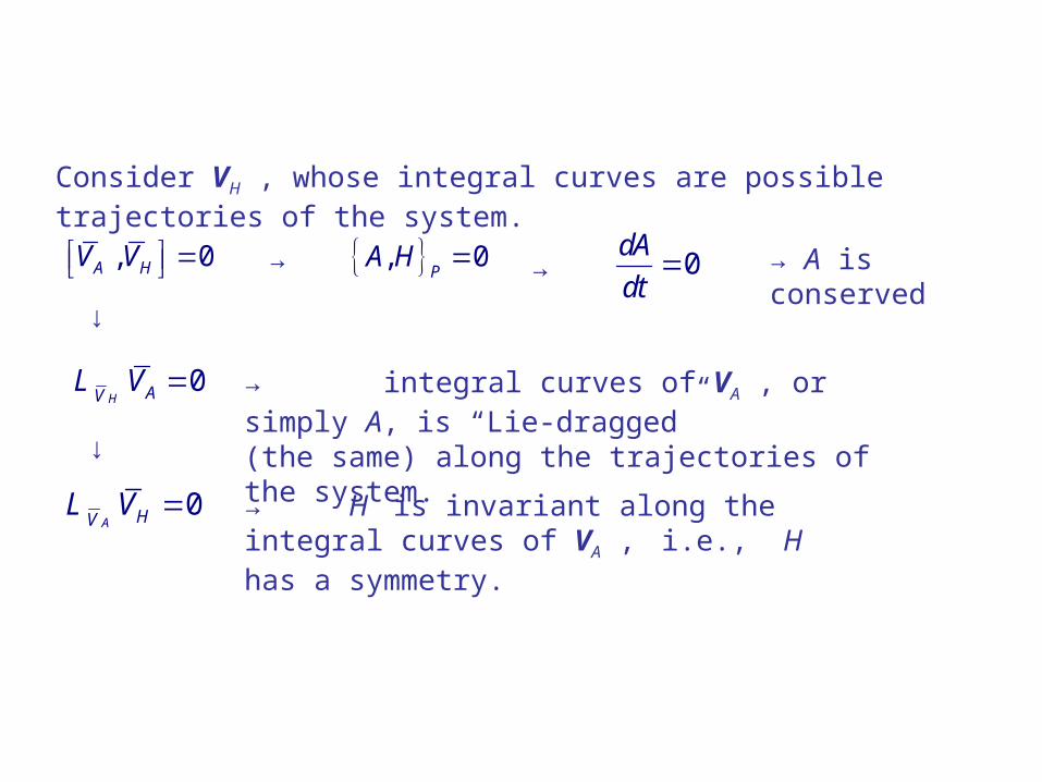
Consider VH , whose integral curves are possible trajectories of the system.

, 0A HV V , 0P

A H → 0dA

dt→ → A is conserved

↓

0H AV

V L → integral curves of VA , or simply A, is “Lie-dragged” (the same) along the trajectories of the system. ↓

0A HV

V L → H is invariant along the integral curves of VA , i.e., H has a symmetry.