DISCHARGE:ARITHMETIC METHOD

CIEN 6011FEBRUARY 2014

OUTLINE

• Field techniques for measuring streamflow

• Computation of discharge

• Exercises

LEARNING OUTCOMES

• Understand the field techniques used for measuring velocity

• Understand various methods of computing discharge

STREAMFLOW METERING USING A CURRENT METER

• Set up a transect

• Measure width of channel

• Determine spacing of velocity readings based on width (verticals)

• Measure velocity based on depth of vertical

• Calculate total discharge (Q) at the transect location

SITE SELECTION• Straight channel with a uniform cross-section

• Laminar flows along transect

• Channels should be free of obstruction, debris and vegetation

• Avoid sites with dead water, turbulent flows, vortices and reverse

flow

• Depth of the water should allow for current measurements at all

river stages

• Ease of access to site

• Located away from pumps, outfalls, sluices and bridges (measure

upstream of the bridge)

MEASURE CHANNEL WIDTH• Choose a point on the bank to start the transect

• Stretch a measuring tape perpendicular to the direction of flow from

one bank to the next

• Secure the measuring tape on both ends (bank reference points)

• Record the channel width of the stream’s water surface

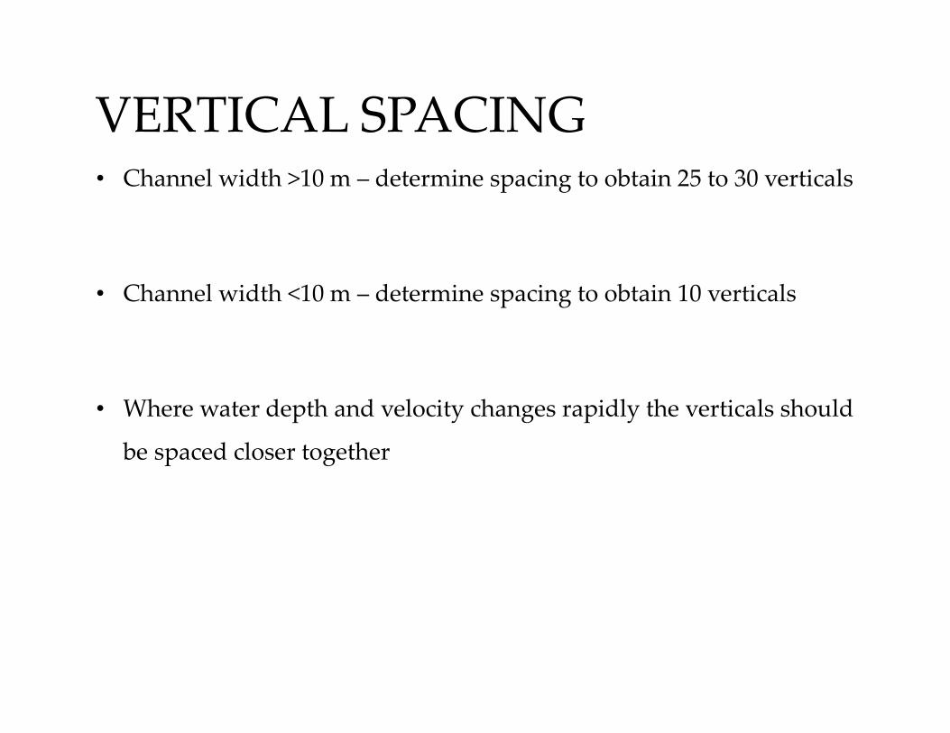
VERTICAL SPACING• Channel width >10 m – determine spacing to obtain 25 to 30 verticals

• Channel width <10 m – determine spacing to obtain 10 verticals

• Where water depth and velocity changes rapidly the verticals should

be spaced closer together

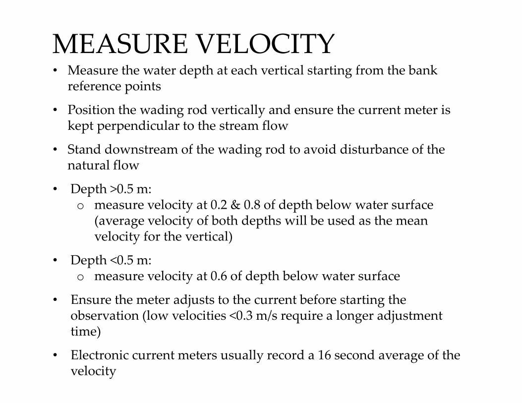
MEASURE VELOCITY• Measure the water depth at each vertical starting from the bank

reference points

• Position the wading rod vertically and ensure the current meter is kept perpendicular to the stream flow

• Stand downstream of the wading rod to avoid disturbance of the natural flow

• Depth >0.5 m:o measure velocity at 0.2 & 0.8 of depth below water surface

(average velocity of both depths will be used as the mean velocity for the vertical)

• Depth <0.5 m:o measure velocity at 0.6 of depth below water surface

• Ensure the meter adjusts to the current before starting the observation (low velocities <0.3 m/s require a longer adjustment time)

• Electronic current meters usually record a 16 second average of the velocity

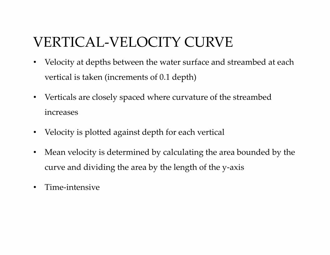
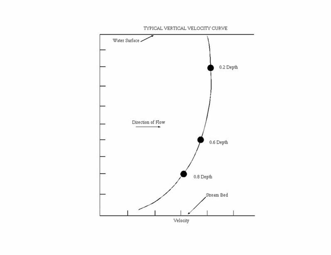
VERTICAL-VELOCITY CURVE

• Velocity at depths between the water surface and streambed at each

vertical is taken (increments of 0.1 depth)

• Verticals are closely spaced where curvature of the streambed

increases

• Velocity is plotted against depth for each vertical

• Mean velocity is determined by calculating the area bounded by the

curve and dividing the area by the length of the y-axis

• Time-intensive

TWO-POINT METHOD

• Velocity measured at 0.2 and 0.8 of the vertical depth

• Mean velocity is calculated as the average of these two readings

• Used for depths >0.5 m

• Test for appropriateness of measuring mean velocity - 0.2 depth

velocity should be greater than 0.8 depth velocity but not more than

double the amount

0.6 DEPTH METHOD

• Velocity measured at 0.6 of the vertical depth is the mean velocity of

the vertical

• Used for channel depths between 0.1 and 0.5 m

• Suitable for changing stage when a quick velocity measurement is

required

0.2 DEPTH METHOD

• Velocity is measured at 0.2 of the vertical depth

• A coefficient is applied to this reading to determine mean velocity.

• Coefficient is derived from the point to mean velocity ratio. USGS

used 0.87.

• Vertical-velocity curves are used to establish a relationship between

mean velocity and velocity at 0.2 of depth.

• Velocity-relation curve is plotted by plotting the true mean versus

the 0.2-depth velocity. Coefficient is derived from this curve

• Used for rivers with high velocity flows

• Not as accurate as the two point or 0.6 depth methods

THREE POINT METHOD

• Velocity is recorded at 0.2, 0.6 and 0.8 of the vertical depth

• The average velocity of 0.2 and 0.8 depths are calculated and then

averaged with the 0.6 depth velocity

• Alternatively, the arithmetic mean of the three velocities can be

reviewed

• Vertical depth >0.5 m

• Used when velocities in a vertical are abnormally distributed due to

turbulence or an obstruction

SURFACE AND SUBSURFACE METHOD

• Surface velocity is measured using a current meter or timing surface

floats

• Subsurface velocity is measured at 0.6 depth or below

• Coefficients are used to convert the surface or subsurface velocities

to mean velocity

• Vertical-velocity curve is used to derive the coefficients

• Coefficients may range from 0.84 to 0.9 based on shape of vertical-

velocity curve:

o Higher coefficients – smooth stream beds and normal shaped curves

o Lower coefficients – irregular stream beds and irregular curves

INTEGRATION METHOD

• Current meter is lowered in the vertical to the streambed and slowly

raised to the surface at a uniform rate

• The total number of revolutions and elapsed time is recorded

• A horizontal axis current meter can only be used since the vertical

movement of the meter will affect the measurements taken using a

vertical axis current meter

• Velocity at the stream bed cannot be measured using this method

• Accuracy dependent on the ability to move the meter at a constant

rate

FIVE POINT METHOD

• Velocity measurements recorded at :

1. 0.22. 0.63. 0.84. Surface5. Streambed

• Velocity measurements plotted on a graph and mean velocity is

determined using a planimeter or equation:

V = 0.1 (Vsurface + 3V0.2 + 3V0.6 + 2V0.8 + Vbed)

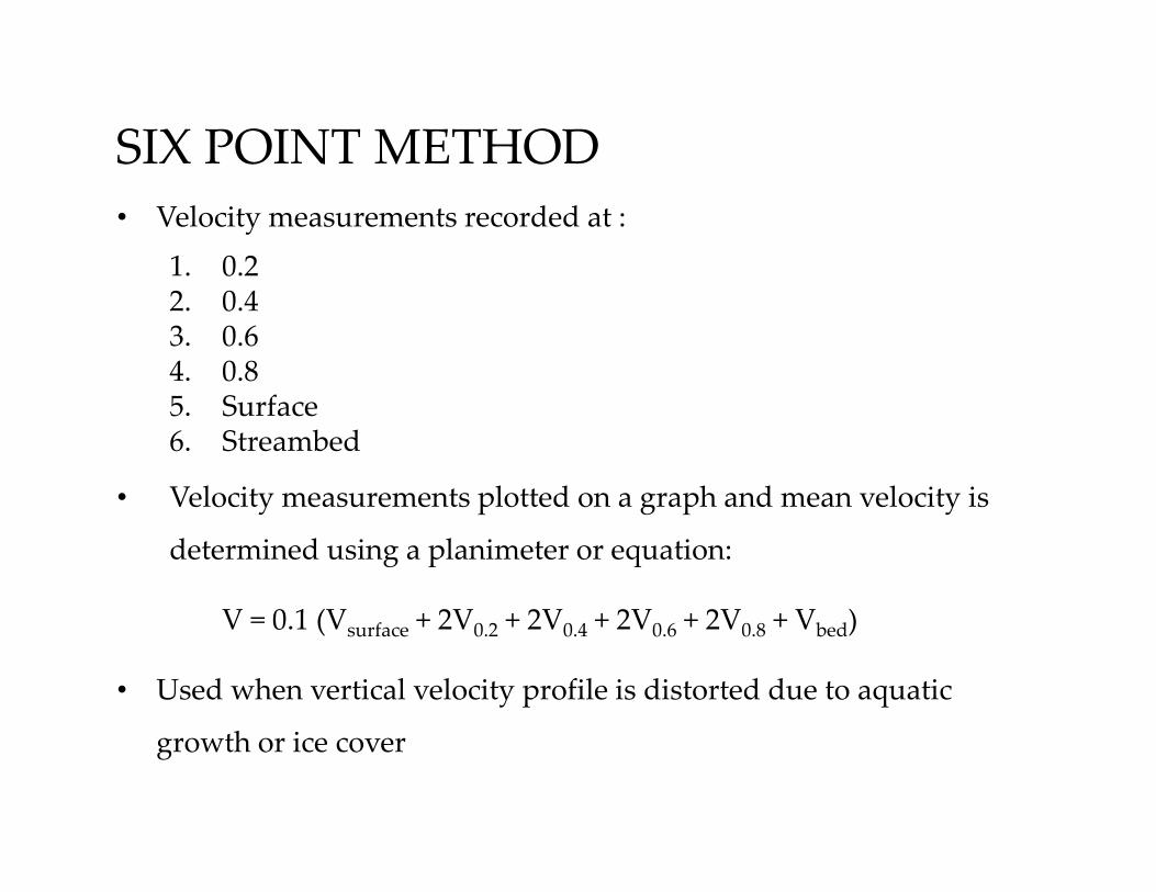
SIX POINT METHOD

• Velocity measurements recorded at :

1. 0.22. 0.43. 0.64. 0.85. Surface6. Streambed

• Velocity measurements plotted on a graph and mean velocity is

determined using a planimeter or equation:

V = 0.1 (Vsurface + 2V0.2 + 2V0.4 + 2V0.6 + 2V0.8 + Vbed)

• Used when vertical velocity profile is distorted due to aquatic

growth or ice cover

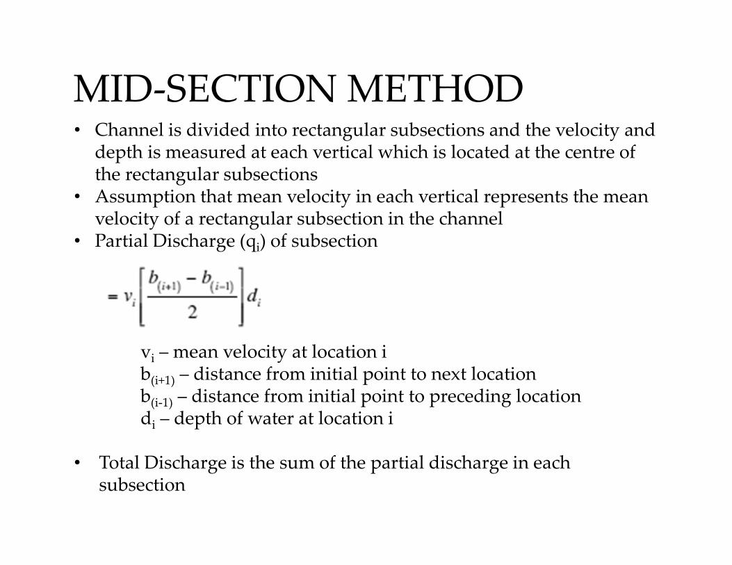
MID-SECTION METHOD• Channel is divided into rectangular subsections and the velocity and

depth is measured at each vertical which is located at the centre of the rectangular subsections

• Assumption that mean velocity in each vertical represents the mean velocity of a rectangular subsection in the channel

• Partial Discharge (qi) of subsection

vi – mean velocity at location ib(i+1) – distance from initial point to next locationb(i-1) – distance from initial point to preceding locationdi – depth of water at location i

• Total Discharge is the sum of the partial discharge in each subsection

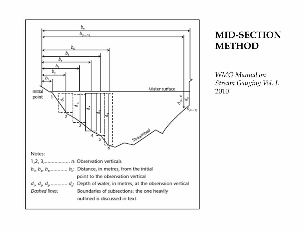
MID-SECTION METHOD

WMO Manual on Stream Gauging Vol. I, 2010

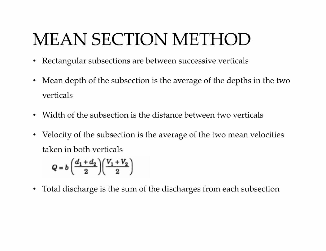
MEAN SECTION METHOD• Rectangular subsections are between successive verticals

• Mean depth of the subsection is the average of the depths in the two

verticals

• Width of the subsection is the distance between two verticals

• Velocity of the subsection is the average of the two mean velocities

taken in both verticals

• Total discharge is the sum of the discharges from each subsection

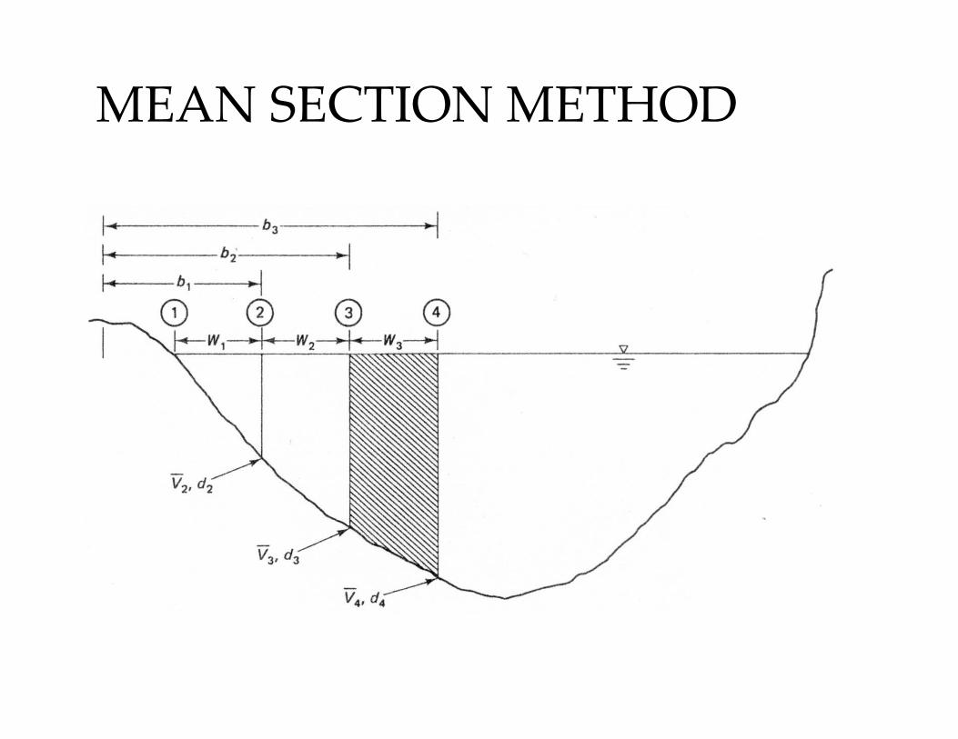
MEAN SECTION METHOD

MANNING’S EQUATION

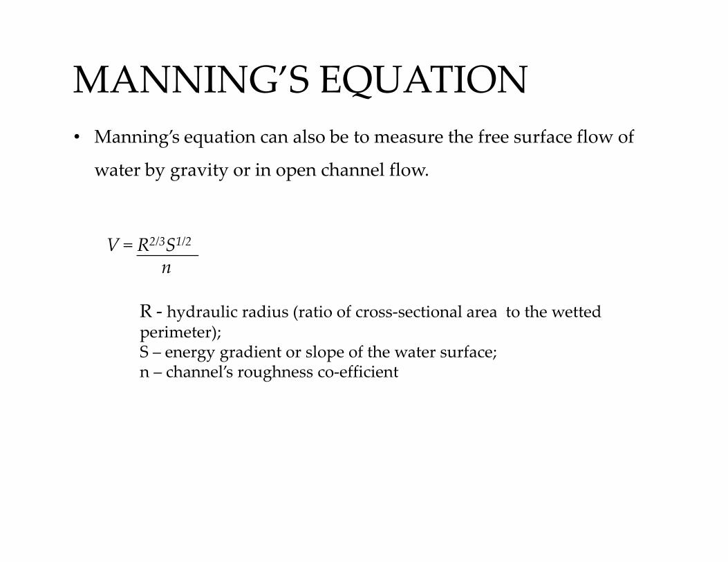
• Manning’s equation can also be to measure the free surface flow of

water by gravity or in open channel flow.

V = R2/3S1/2

n

R - hydraulic radius (ratio of cross-sectional area to the wetted perimeter); S – energy gradient or slope of the water surface; n – channel’s roughness co-efficient

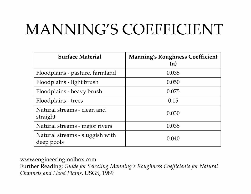
MANNING’S COEFFICIENT

Surface Material Manning’s Roughness Coefficient (n)

Floodplains - pasture, farmland 0.035

Floodplains - light brush 0.050

Floodplains - heavy brush 0.075

Floodplains - trees 0.15

Natural streams - clean and straight

0.030

Natural streams - major rivers 0.035

Natural streams - sluggish with deep pools

0.040

www.engineeringtoolbox.comFurther Reading: Guide for Selecting Manning’s Roughness Coefficients for Natural Channels and Flood Plains, USGS, 1989