3. Basics of Heat Transfer

Course Part A: Introduction to Electronics Cooling

MPE 635: Electronics Cooling 36

3. Basics of Heat Transfer This lecture is intended to refresh the post graduate students memory about the basics of heat transfer regarding the various modes of heat transfer, analogy between heat transfer and electric circuits, combined modes of heat transfer and the overall heat transfer coefficient. As a start, we will begin by the modes of heat transfer mechanism in a brief review then we will elaborate on the analogy between heat transfer and electric circuits. This will enable us to study the combined modes of heat transfer then we will end this lecture with the concept of overall heat transfer coefficient.

3.1 Modes of Heat Transfer Heat, by definition, is the energy in transit due to temperature difference. Whenever exists a temperature difference in a medium or between media, heat flow must. Different types of heat transfer processes are called modes. These modes are shown in Figure 3.1. When a temperature gradient exists in a stationary medium, which may be a solid or a fluid, heat flows under the law of conduction heat transfer. On the other hand if the temperature gradient exists between a surface and a moving fluid we use the term Convection. The third mode of heat transfer is termed Radiation and it needs no medium to transfer through since it is driven by electromagnetic waves emitted from all surfaces of finite temperature, so there is a net heat transfer by radiation between two surfaces at different temperatures.

Figure 3.1 Conduction, convection and radiation heat transfer modes

3.1.1 Conduction Conduction is the mechanism of heat transfer whereby energy is transported between parts of a continuum by the transfer of kinetic energy between particles or groups of particles at the atomic level. We should conjure up the concept of atomic and molecular activity In gases,



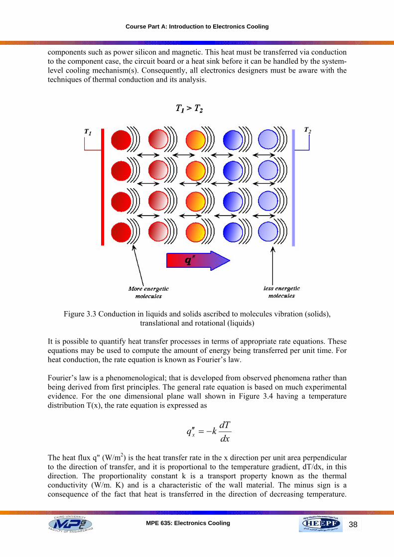
conduction is caused by elastic collision of molecules; consider a gas in which there exist a temperature gradient and assume there is no bulk motion . The gas may occupy the space between two surfaces which are maintained at different temperatures as shown in Figure 3.2. We associate the temperature at any point with the energy of gas molecules in proximity to the point. This energy is related to the random translational motion as well as to the internal rotational and vibrational motions of the molecules. As shown in Figure 3.3. The hypothetical plane at xo is constantly being crossed by molecules from above and below due to their random motion. However, molecules from above are associated with a larger temperature than those from below, causing net transfer of energy in the positive x direction. We may speak of the net transfer of energy by the random molecular motion as a diffusion of energy.

Figure 3.2 Conduction heat transfer as diffusion of energy due to molecular activity. In liquids and electrically non conducting solids, it is believed to be caused by longitudinal oscillations of the lattice structure; it is called also lattice waves. Thermal conduction in metals occurs, like electrical conduction, through the motion of free electrons. Thermal energy transfer occurs in the direction of decreasing temperature, a consequence of the second law of thermodynamics. In solid opaque bodies, thermal conduction is the significant heat transfer mechanism because no net material flows in the process. With flowing fluids, thermal conduction dominates in the region very close to a solid boundary, where the flow is laminar and parallel to the surface and where there is no eddy motion. Examples of conduction heat transfer are tremendous. On a summer day there is a significant energy gain from outside air to a room. This gain is principally due to conduction heat transfer through the wall that separates room air from outside air. Also in electronics cooling process conduction is a heat transfer mechanism used in every electronics design. Even if a system is designed for convection cooling of the circuit boards, conduction is still the dominant heat transfer mechanism within the component devices and on the circuit board. This is especially true for power electronics, where concentrations of heat are developed in



components such as power silicon and magnetic. This heat must be transferred via conduction to the component case, the circuit board or a heat sink before it can be handled by the system-level cooling mechanism(s). Consequently, all electronics designers must be aware with the techniques of thermal conduction and its analysis.

Figure 3.3 Conduction in liquids and solids ascribed to molecules vibration (solids), translational and rotational (liquids)

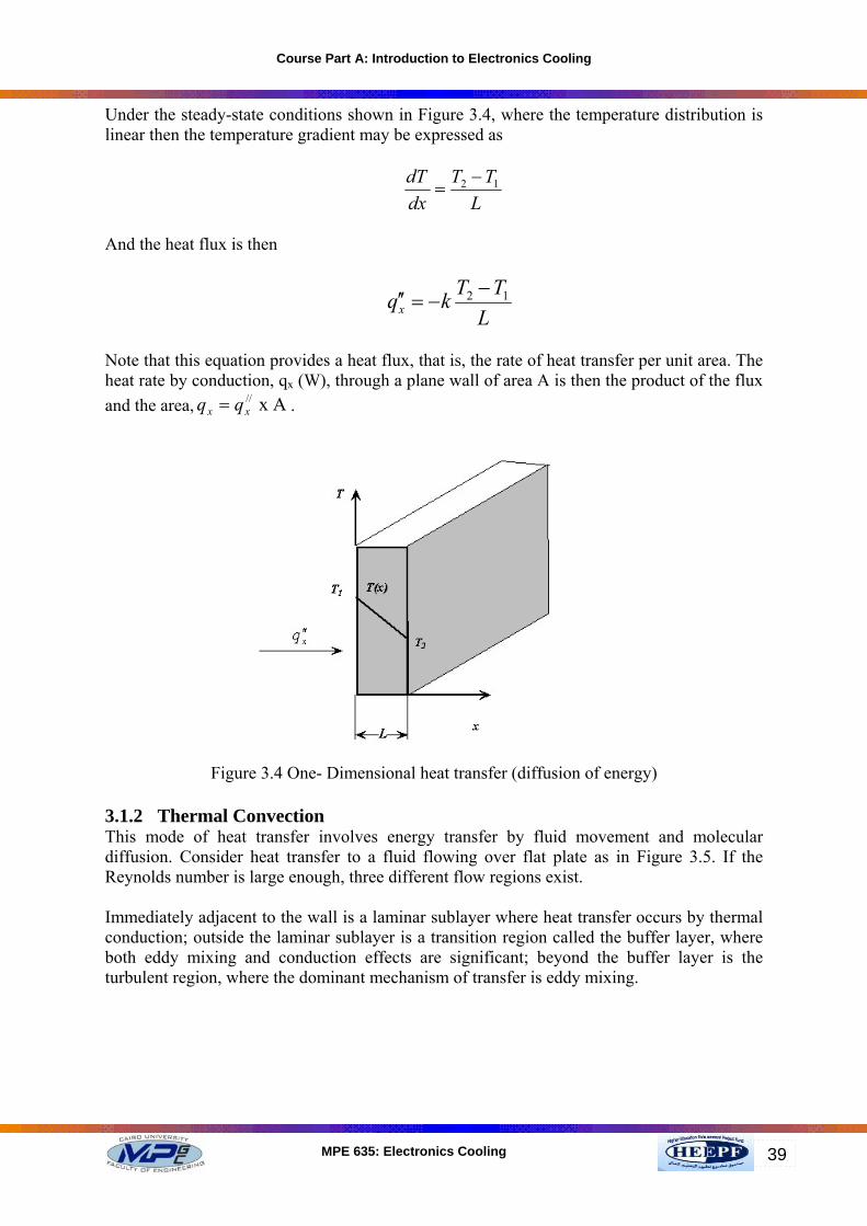
It is possible to quantify heat transfer processes in terms of appropriate rate equations. These equations may be used to compute the amount of energy being transferred per unit time. For heat conduction, the rate equation is known as Fourier’s law. Fourier’s law is a phenomenological; that is developed from observed phenomena rather than being derived from first principles. The general rate equation is based on much experimental evidence. For the one dimensional plane wall shown in Figure 3.4 having a temperature distribution T(x), the rate equation is expressed as

dxdTkqx −=′′

The heat flux q" (W/m2) is the heat transfer rate in the x direction per unit area perpendicular to the direction of transfer, and it is proportional to the temperature gradient, dT/dx, in this direction. The proportionality constant k is a transport property known as the thermal conductivity (W/m. K) and is a characteristic of the wall material. The minus sign is a consequence of the fact that heat is transferred in the direction of decreasing temperature.



Under the steady-state conditions shown in Figure 3.4, where the temperature distribution is linear then the temperature gradient may be expressed as

LTT

dxdT 12 −=

And the heat flux is then

LTTkqx

12 −−=′′

Note that this equation provides a heat flux, that is, the rate of heat transfer per unit area. The heat rate by conduction, qx (W), through a plane wall of area A is then the product of the flux and the area, A x //

xx qq = .

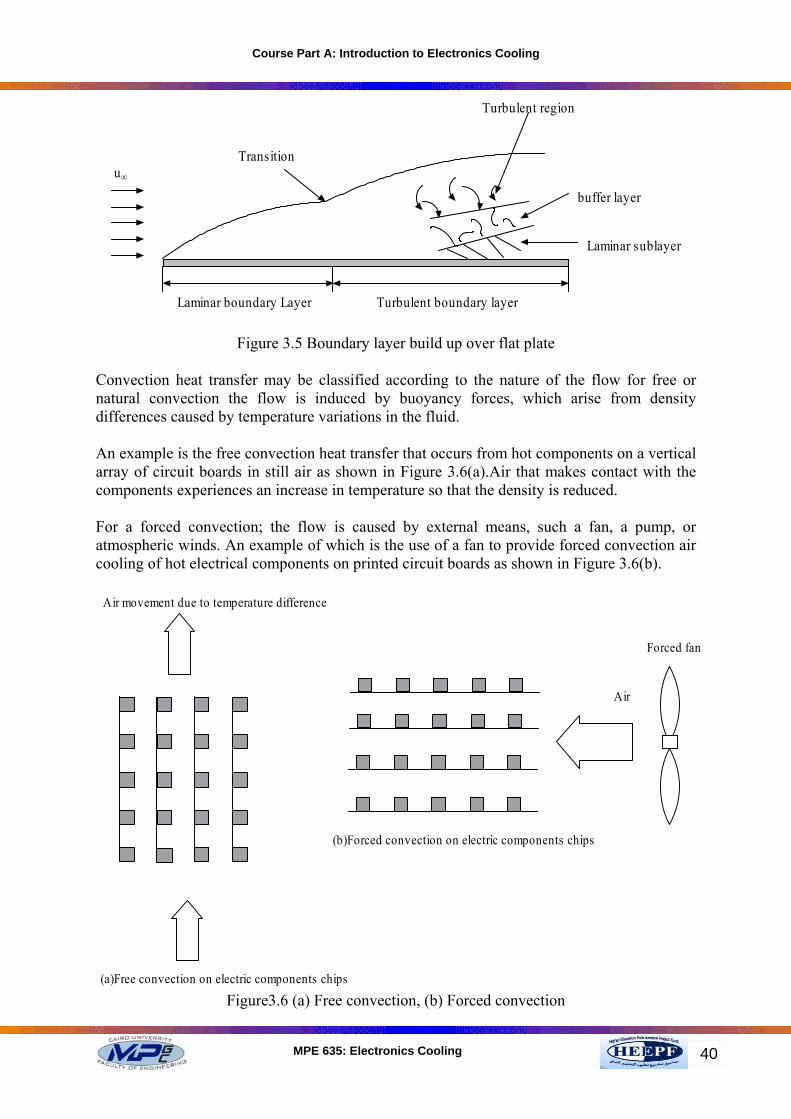
Figure 3.4 One- Dimensional heat transfer (diffusion of energy) 3.1.2 Thermal Convection This mode of heat transfer involves energy transfer by fluid movement and molecular diffusion. Consider heat transfer to a fluid flowing over flat plate as in Figure 3.5. If the Reynolds number is large enough, three different flow regions exist. Immediately adjacent to the wall is a laminar sublayer where heat transfer occurs by thermal conduction; outside the laminar sublayer is a transition region called the buffer layer, where both eddy mixing and conduction effects are significant; beyond the buffer layer is the turbulent region, where the dominant mechanism of transfer is eddy mixing.



Laminar sublayer

buffer layer

Turbulent region

Laminar boundary Layer Turbulent boundary layer

Transitionu∞

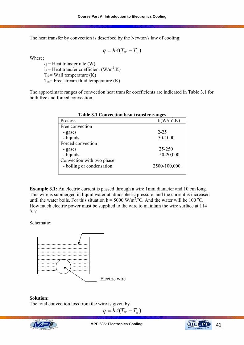
Figure 3.5 Boundary layer build up over flat plate Convection heat transfer may be classified according to the nature of the flow for free or natural convection the flow is induced by buoyancy forces, which arise from density differences caused by temperature variations in the fluid. An example is the free convection heat transfer that occurs from hot components on a vertical array of circuit boards in still air as shown in Figure 3.6(a).Air that makes contact with the components experiences an increase in temperature so that the density is reduced. For a forced convection; the flow is caused by external means, such a fan, a pump, or atmospheric winds. An example of which is the use of a fan to provide forced convection air cooling of hot electrical components on printed circuit boards as shown in Figure 3.6(b).

Air movement due to temperature difference

(a)Free convection on electric components chips

Air

(b)Forced convection on electric components chips

Forced fan

Figure3.6 (a) Free convection, (b) Forced convection



The heat transfer by convection is described by the Newton's law of cooling:

)( ∞−= TThAq W Where;

q = Heat transfer rate (W) h = Heat transfer coefficient (W/m2.K) Tw= Wall temperature (K) T∞= Free stream fluid temperature (K)

The approximate ranges of convection heat transfer coefficients are indicated in Table 3.1 for both free and forced convection.

Table 3.1 Convection heat transfer ranges Process h(W/m2.K) Free convection - gases 2-25 - liquids 50-1000 Forced convection - gases 25-250 - liquids 50-20,000 Convection with two phase - boiling or condensation 2500-100,000

Example 3.1: An electric current is passed through a wire 1mm diameter and 10 cm long. This wire is submerged in liquid water at atmospheric pressure, and the current is increased until the water boils. For this situation h = 5000 W/m2.oC. And the water will be 100 oC. How much electric power must be supplied to the wire to maintain the wire surface at 114 oC? Schematic:

Solution: The total convection loss from the wire is given by

)( ∞−= TThAq W

Electric wire



For this problem the surface area of the wire is A= π d L = π (1 x 10-3) (10 x 10-2) = 3.142 x10-4 m2

The heat transfer is therefore Wq 99.21)100114(10142.35000 4 =−×××= −

And this is equal to the electric power which must be applied. 3.1.3 Thermal Radiation The mechanism of heat transfer by radiation depends on the transfer of energy between surfaces by electromagnetic waves in wave length interval between 0.1 to 100 µm. Radiation heat transfer can travel in vacuum such as solar energy. Radiation heat transfer depends on the surface properties such as colors, surface orientation and fourth power of the absolute temperature (T4) of the surface. The basic equation for radiation heat transfer between two gray surfaces is given by:

)( 42

41 TTfAq −= σε

Where: σ = Stefan-Boltzmann constant = 5.67x10-8 W/m2.K4 ε = Emissivity of the surface which provide of how efficiently a surface emits energy relative to a black body(no reflection) and it's ranges 0≤ ε ≤1 ƒ = Geometrical factor which depends on the orientation between the surfaces Example3.2: A horizontal steel pipe having a diameter of 10 cm is maintained at a temperature of 60 oC in a large room where the air and wall temperature are at 20 oC with average heat transfer coefficient 6.5 W/m2.k. The emissivity of the steel is 0.6 calculate the total heat lost from the pipe per unit length. Solution: The total heat lost from the pipe due to convection and radiation

)()( 44∞∞ −+−=

+=

TTfATTAh

qqq

SS

radiationconvectiontotal

σε Because the pipe in a large enclosure then the geometrical factor ƒ = 1

mWxxxqtotal

/33.134)293333)(1.0)(1)(6.0(1067.5)2060)(1.0(5.6 448

=−+−= − ππ

3.2 Analogy between Heat Transfer and Electric Circuits There exists an analogy between the diffusion of heat and electrical charge. Just as an electrical resistance is associated with the conduction of electricity, a thermal resistance may be associated with the conduction of heat. Defining resistance as the ratio of a driving potential to the corresponding transfer rate, it follows from Figure 3.4 that the thermal resistance for conduction is:



kAL

qTT

Rx

sscondt =

−≡ 2,1,

,

As the electric resistance from Ohm’s law

AL

IEE

R sse σ

=−

= 2,1,

As there is a conduction resistance also there is a convection resistance.

q = h A (Ts- T∞)

hAqTTR s

convt1

, =−

≡ ∞

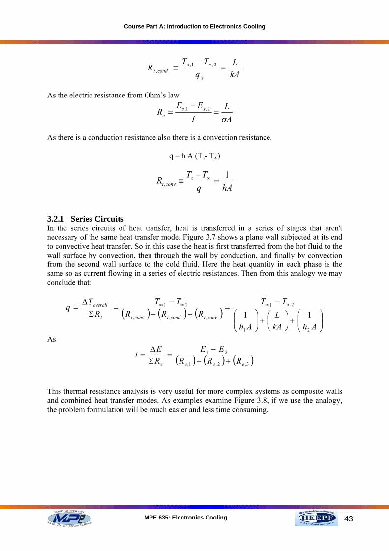
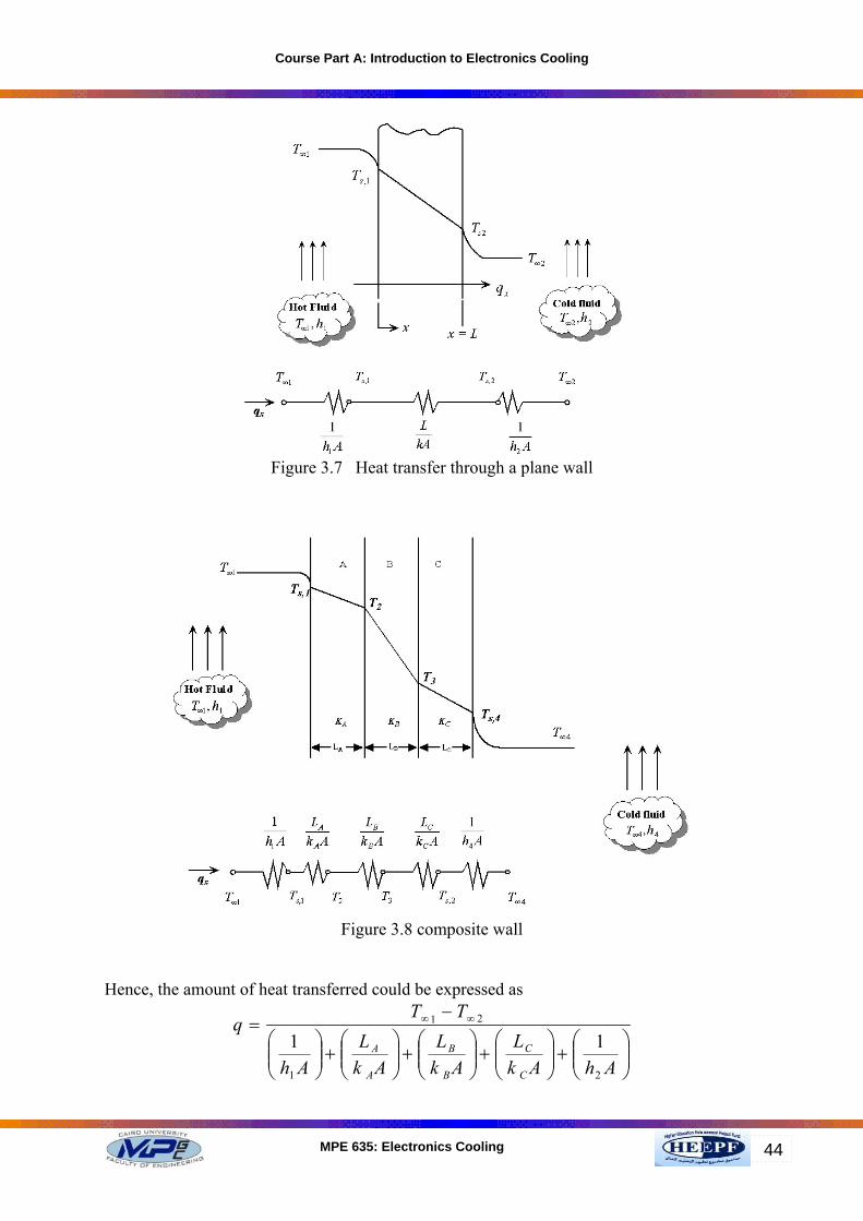
3.2.1 Series Circuits In the series circuits of heat transfer, heat is transferred in a series of stages that aren't necessary of the same heat transfer mode. Figure 3.7 shows a plane wall subjected at its end to convective heat transfer. So in this case the heat is first transferred from the hot fluid to the wall surface by convection, then through the wall by conduction, and finally by convection from the second wall surface to the cold fluid. Here the heat quantity in each phase is the same so as current flowing in a series of electric resistances. Then from this analogy we may conclude that:

( ) ( ) ( )⎟⎟⎠

⎞⎜⎜⎝

⎛+⎟

⎠⎞

⎜⎝⎛+⎟⎟

⎠

⎞⎜⎜⎝

⎛−

=++

−=

Σ∆

= ∞∞∞∞

AhkAL

Ah

TTRRR

TTR

Tqconvtcondtconvtt

overall

21

21

,,,

21

11

As

( ) ( ) ( )3,2,1,

21

eeee RRREE

REi

++−

=Σ∆

=

This thermal resistance analysis is very useful for more complex systems as composite walls and combined heat transfer modes. As examples examine Figure 3.8, if we use the analogy, the problem formulation will be much easier and less time consuming.



Figure 3.7 Heat transfer through a plane wall

Figure 3.8 composite wall

Hence, the amount of heat transferred could be expressed as

⎟⎟⎠

⎞⎜⎜⎝

⎛+⎟⎟

⎠

⎞⎜⎜⎝

⎛+⎟⎟

⎠

⎞⎜⎜⎝

⎛+⎟⎟

⎠

⎞⎜⎜⎝

⎛+⎟⎟

⎠

⎞⎜⎜⎝

⎛−

= ∞∞

AhAkL

AkL

AkL

Ah

TTq

C

C

B

B

A

A

21

21

11



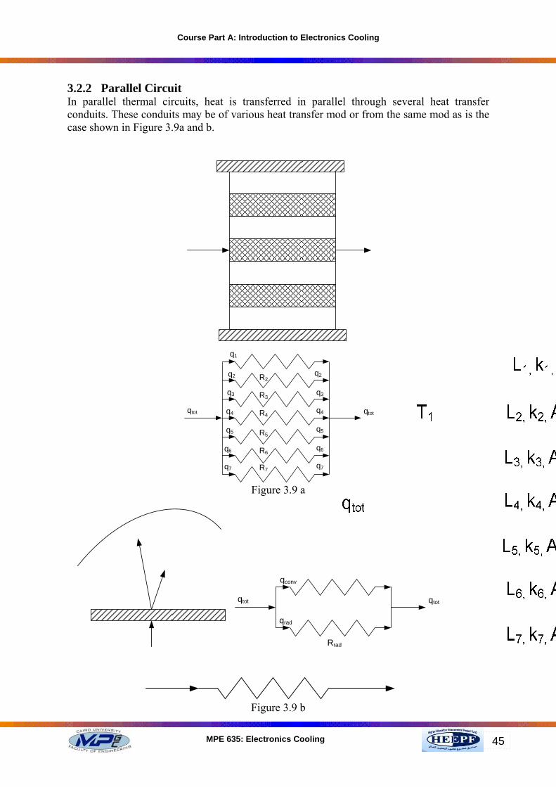
3.2.2 Parallel Circuit In parallel thermal circuits, heat is transferred in parallel through several heat transfer conduits. These conduits may be of various heat transfer mod or from the same mod as is the case shown in Figure 3.9a and b.

q1

qtot qtot

q7

q6

q7

q5

q6

q4

q5

q3 q3

q2 q2

R7

R6

R5

R3

R2

R4q4

Figure 3.9 a

qtot qtot

qrad

qconv

Rrad

Figure 3.9 b



Now considering the case in Figure 3.9 a,

itiiii R

TLTAkq

,

∆=

∆=

And;

totttttttttitot R

TRRRRRRR

Tqq,7,6,5,4,3,2,1,

1111111 ∆=⎟

⎟⎠

⎞⎜⎜⎝

⎛++++++∆=Σ=

This means that like electric circuits in parallel, the equivalent total thermal resistance would be:

∑=ittott RR ,,

11

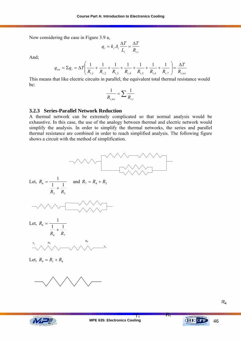
3.2.3 Series-Parallel Network Reduction A thermal network can be extremely complicated so that normal analysis would be exhaustive. In this case, the use of the analogy between thermal and electric network would simplify the analysis. In order to simplify the thermal networks, the series and parallel thermal resistance are combined in order to reach simplified analysis. The following figure shows a circuit with the method of simplification.

Let,

32

6 111

RR

R+

= and 547 RRR +=

Let,

76

8 111

RR

R+

=

T1

T2

R8R1

Let, 819 RRR +=



3.3 Combined Modes of Heat Transfer Most of the practical cases under investigations, heat is transferred by more than one mode; as for examples heat may be transferred by combined convection and radiation, combined convection and conduction, etc. 3.3.1 Combined Convection and Radiation Since these two modes of heat transfer are completely independent, there would be no mutual effect between them. Thus net heat exchange of the surface is the sum of the two

radconvnet qqq +=

This hypothetical approach seems to be similar to the parallel electrical resistances as shown previously, but the problem here is that no radiation resistance has been defined yet. So let us use a radiant heat transfer in order to express the radiation heat transfer, q rad, as a linear function in the temperature difference between the surface temperature and the fluid temperature.

)( fsrrad TTAhq −××= Where; hr = radiation heat transfer coefficient, W/m2.K A = heat transfer surface area, m2 Ts = surface absolute temperature, K Tf = enclosure absolute temperature, K Now it is time to define how the radiation heat transfer coefficient can be obtained

)()(

)(

44

fs

esse

fs

radr TT

TTF

TTAq

h−−

×××=−×

= σε

In the above equation, Te is used to express the enclosure temperature as this is the more general case. But for most of the cases, the fluid adjacent to the surface has the same temperature as that of the enclosure. So for this most likely circumstance the following agree:

)()()()(

)()( 2244

fs

fsfsfsse

fs

fsser TT

TTTTTTF

TTTT

Fh−

−×+×+×××=

−

−×××= σεσε

)()2)(()()( 222

fsfsfssefsfsser TTTTTTFTTTTFh +×−+×××=+×+×××=∴ σεσε Now if we define the arithmetic means temperature as

2fs

m

TTT

+=

If further Ts-Te<<Ts then

fsm TTT = So we may define the radiation heat transfer coefficient as



34 mser TFh ××××=∴ σε And finally;

)( fstotnet TTAhq −××= . Where radconvtot hhh += 3.3.2 Combined Convection and Conduction This combination is likely to occur with the use of extended surfaces where the primary surface exchanges heat by convection to the adjacent fluid flow and by conduction through the extended surfaces. This case may be considered in a similar manner as the above, but here the problem doesn't need extra work as the conduction thermal resistance is pre-defined.

condconvnet qqq +=

ALTT

kTThq extsfsconvnet ×⎟

⎠⎞

⎜⎝⎛ −

+−=)(

)(

3.4 Overall Heat Transfer Coefficient The concept of overall heat transfer coefficient laid its importance in the heat exchanger design and industry as it combines the various modes of heat transfer in the heat exchange between two fluids. The concept of overall heat transfer has been extensively studied in the undergraduate courses of heat transfer and heat transfer equipments, but again for reasons of memory refresh. Let's examine the defining equation and it parameters.

)(1

)()()(1

1

,,,,,,

",

,,,

",

,,, shhfphhshhfph

hf

msccfpc

cf

sccfpcc

cchh

AAhAAR

kAx

AAR

AAh

AUAU

ηηηη ++

+++

++

+

==

Where; Uc is the overall heat transfer coefficient based on the cold side area, W/m2.K. Ac is the total heat transfer surface area adjacent to the cold fluid side, m2. Uh is the overall heat transfer coefficient based on the hot side area, W/m2.K. Ah is the total heat transfer surface area adjacent to the hot fluid side, m2. hc is the convection heat transfer coefficient based on the cold side area, W/m2.K. Ac,p is the primary heat transfer surface area adjacent to the cold fluid side, m2. Ac,s is the secondary heat transfer surface area adjacent to the cold fluid side, m2. ηf,c is the cold side fin efficiency. Rf,c

" is the fouling factor for the cold side, m2.K/W. x is the wall thickness, m. k is the thermal conductivity of the interface wall material, W/m2.K. Am mean heat transfer area for conduction, m2. hh is the convection heat transfer coefficient based on the hot side area, W/m2.K. Ah,p is the primary heat transfer surface area adjacent to the hot fluid side, m2. Ah,s is the secondary heat transfer surface area adjacent to the hot fluid side, m2.



ηf,h is the hot side fin efficiency. Rf,h

" is the fouling factor for the hot side, m2.K/W. The following table gives values for representative fouling factor for several applications: The heat transfer between to fluids separated by heat transfer area can then be easily calculated as:

overallhhnet TAUQ ∆= The following table shows some values for the overall heat transfer coefficient:

Fluid Rf,", m2.K/W.

Seawater and treated boiler feedwater (below 50 ºC)

0.0001

Seawater and treated boiler feedwater (above50 ºC)

0.0002

River water below 50 ºC 0.0002-0.001 Fuel oil 0.0009 Refrigerating liquids 0.0002 Steam (nonoil bearing) 0.0001

Fluid combination U, W/m2.K.

Water to water 850-1700 Water to oil 110-350 Steam condenser, water in tube 1000-6000 Ammonia condenser, water in tube 800-1400 Finned tube heat exchanger, water in tubes air in cross flow

25-50

Documents

3. Basics of Heat Transfer