1

Second Year Project Report

Mode Division Multiplexed Transmission for Long Haul Fiber

Communication Systems

April 2014

By:

Hamdi Ghodbane

Saddam Gafsi

Supervisors:

Dr. Amine Ben Salem

Pr. Mourad Zghal

2

Acknowledgements

We wish to express our sincere gratitude and appreciation to everyone who assisted

and supported us during this project. We would like to make special mention of the following

people:

Our supervisor, Professor Mourad ZGHAL, first for giving us the opportunity to work

on such an exciting subject in the field of optics, the field we were passionate about and

aspired to work in, second for his encouragement and appreciation for our efforts, and finally

for introducing us to great people that we now enjoy their friendship and look forward to

further work with.

Our second supervisor doctor Amine Ben Salem for his continuous support, his

guidings, although some times strict have always been in our best interest.

Finally, we would like to thank our friend and colleague Abderrahmen trichilli for his

valuable help and encouragement during this project.

3

Table of contents

General introduction :................................................................................................................................................. 9

1. Chapter 1 : The capacity crunch and the need for new multiplexing techniques ............................ 11

1.1 Introduction : ................................................................................................................................................... 11

1.2 Motivation : ...................................................................................................................................................... 11

1.3 Existing multiplexing techniques : ............................................................................................................. 12

1.3.1 Wavelength division multiplexing :........................................................................................... 12

1.3.2 Time division multiplexing : ........................................................................................................ 12

1.3.3 Polarization division multiplexing : ...........................................................................................13

1.3.4 Code division multiplexing : ........................................................................................................13

1.3.5 Subcarrier multiplexing : ..............................................................................................................13

1.4 Space Division Multiplexing : ......................................................................................................................14

1.4.1 Overview :...............................................................................................................................................14

1.4.2 Presentation of optical fibers :.....................................................................................................14

1.4.3 Concept of SDM : ........................................................................................................................... 15

1.4.4 Engineering challenges and current state : .............................................................................. 17

1.5 Conclusion : ......................................................................................................................................................19

2. Chapter 2 : Modes determination and optical fiber modeling ............................................................... 20

2.1 Introduction : ................................................................................................................................................... 20

2.2 Optical Fiber Modes Determination : ......................................................................................................... 20

2.2.1 Maxwell’s equations : ............................................................................................................................. 20

2.2.3 Bessel Equation : .....................................................................................................................................23

2.2.4 Mode determination: .............................................................................................................................. 27

2.2.5 Solutions for m=0 and m=1 : ................................................................................................................ 28

2.2.6 Solutions for m>1 : ..................................................................................................................................30

2.2.7 Field amplitude distribution of the modes: .......................................................................................31

2.2.8 Analogy with microwave waveguides: ..............................................................................................33

2.3 Modeling the optical fiber : ..........................................................................................................................34

2.4 Conclusion : ......................................................................................................................................................36

3. Chapter 3 : Study of key system performance parameters in a MDM transmission system .........37

3.1 Introduction : ...................................................................................................................................................37

3.2 Definition and perspective : .........................................................................................................................37

3.3 Mode coupling and its origins : ..................................................................................................................38

3.4 Coupled power theory : .................................................................................................................................38

3.5 Simulation and parametric study: ...............................................................................................................41

3.5.1 Justification of the perturbation model : ...........................................................................................41

4

3.5.2 Refractive index perturbation : ............................................................................................................ 45

3.5.3 Input powers : .......................................................................................................................................... 48

3.5.4 Core radius : ............................................................................................................................................. 50

3.5.5 Wavelength : ............................................................................................................................................ 50

3.5.6 Modes : ....................................................................................................................................................... 51

3.5.7 Coupling of modes of the same group: .............................................................................................. 51

3.5.8 Effect of the number of modes : .......................................................................................................... 52

3.6 Conclusion : ...................................................................................................................................................... 58

Conclusion : ................................................................................................................................................................. 58

4. Bibliography : .................................................................................................................................................... 60

5

List of figures

Figure 1 Forecast of the worldwide IP traffic in petabytes per month, according to the Cisco Visual Networking Index ...................................................................................................................................................... 11 Figure 2 Multimode and single mode fibers ........................................................................................................14 Figure 3 Multicore fibers .......................................................................................................................................... 15 Figure 4 SDM over a few mode fiber ....................................................................................................................16 Figure 5 SDM over a multicore fiber .....................................................................................................................16 Figure 6 Cylindrical coordinate system ................................................................................................................ 24 Figure 7 solutions of the eigenvalue equation for m=0 in the (u,w) plane .................................................. 29 Figure 8 solutions of the eigenvalue equation for m=0 and m=1 in the (u,w) plane ................................30 Figure 9 Field intensity distribution for m=0 ......................................................................................................32 Figure 10 Field intensity distribution for m=1 Figure 11 Field intensity distribution for m=2 ................................................................................................................................32 Figure 12 correspondence between modes in metallic guides and optical fibers ......................................33 Figure 13 Dividing a sphere into smaller finite elements (meshing) progressively .................................34 Figure 14 Different types of finite elements that can be used in meshing ..................................................34 Figure 15 Meshed structure .....................................................................................................................................35 Figure 16 calculated solution ..................................................................................................................................35 Figure 17. LP11 mode : transverse electric field and electric field norm .......................................................41 Figure 18. LP01 mode : transverse electric field and electric field norm .......................................................41 Figure 19 3D plot of the sin(2x)*cos(2y) function .............................................................................................. 42 Figure 20 Evolution of the perturbed refractive index as a function of the distance z ............................ 42 Figure 21 Evolution of the refractive index of the fiber as a function of the distance z for a higher perturbation value .....................................................................................................................................................43 Figure 22 Exact plot of the fiber’s cross section (5.5 um core radius) ...........................................................43 Figure 23 zoomed-in snapshot of the exact plot of the fiber’s cross section (5.5 um core radius) ........44 Figure 24 Power coupling for δn2(x, y) = 1.5 *10^-2 sin(rc x)cos(rc y) .........................................................44 Figure 25 Crosstalk between the two propagating modes............................................................................... 45 Figure 26 Coupling coefficient as a function of K .............................................................................................46 Figure 27 Point of equilibrium as a function of K ..............................................................................................46 Figure 28 Power coupling for δn2(x, y) = 10^-2 sin(rc x)cos(rc y) ................................................................. 47 Figure 29 Power coupling for δn2(x, y) = 2*10^-2 sin(rc x)cos(rc y) ............................................................. 47 Figure 30 Point of equilbrium as a function of P01 ........................................................................................... 48 Figure 31 Power coupling for P01=4mW and P11=1mW .................................................................................49 Figure 32 Power coupling for P01=1.2mW and P11=1mW .............................................................................49 Figure 33 Coupling coefficient as a function of the core radius .................................................................... 50 Figure 34 Coupling coefficients of the different modes with the fundamental mode .............................. 51 Figure 35 Power coupling between the LP02 and the LP21 modes ............................................................... 52 Figure 36 Power coupling in a four mode fiber .................................................................................................. 54 Figure 37 Power coupling in a six mode fiber (first configuration) .............................................................. 55 Figure 38 Power coupling in a six mode fiber (second configuration) ....................................................... 56 Figure 39 Power coupling in a six mode fiber (third configuration) ............................................................ 56 Figure 40 Power coupling in a six mode fiber (fourth configuration) ......................................................... 57 Figure 41 Power coupling in a six mode fiber (fifth configuration) ............................................................. 57

6

List of tables Table1.1: State of the art SDM demonstrations 18

Table 2.1: Determination of possible solutions 28

Table 3.1: Modes effective indices 54

Table 3.2: Coupling coefficients for the different modes 54

7

List of acronyms: SMF single mode fiber

MMF multimode fiber

FMF few mode fiber

GI graded index fiber

SI step index fiber

WDM wavelength division multiplexing

DWDM dense wavelength division multiplexing

CWDM coarse wavelength division multiplexing

TDM time division multiplexing

FDM frequency division multiplexing

PDM polarization division multiplexing

CDM code division multiplexing

CDMA code division multiple access

SCM subcarrier multiplexing

CATV cable television

SDM spatial division multiplexing

MCF multicore fiber

Tx transmitter

Rx receiver

DSP digital signal processing

FEM finite element method

DMGD differential mode group delay

MIMO multi-input/multi-output

EDFA erbium doped fiber amplifier

8

List of symbols : ∇ : Nabla operator

𝛽 : Propagation constant

휀0 : Vacuum dielectric permittivity

𝜇0 ∶ Vacuum magnetic permiability

𝜆 : wavelength

𝜔 : Anguler frequency

�⃗� : Electric field

�⃗⃗� : Magnetic field

�⃗� : Magnetic induction

�⃗� : Polarization vector

𝑐 : Light celerity in vacuum

𝐽𝑚: 1st order Bessel function

𝐾𝑚 : Modified Bessel function

𝑁𝑚 : Bessel function of the 2nd kind

𝑅𝑒(𝑧) : Real part of the complex number z

𝐼𝑚(𝑧) : Imaginary part of the complex number z

𝑉 : Normalized frequency

𝑘0 : Wavenumber

ℎ𝑝𝑞 : Coupling coefficient between modes p and q

𝜅 : Transverse component of the wavenumber 𝑘0

𝑎: Core radius

𝑛𝑐𝑙 : Refractive index inside the claddinng

𝑛𝑐𝑜: Refractive index inside the core

9

General introduction :

Over the past forty years, a series of technological breakthroughs have allowed the

capacity-per-fiber to increase around 10x every four years. Transmission technology has

therefore thus far been able to keep up with the relentless, exponential growth of capacity

demand. The cost of transmitting exponentially more data was also manageable, in large

part because more data was transmitted over the same fiber by upgrading equipment at the

fiber ends. But in the coming decade or so, an increasing number of fibers in real networks

will reach their capacity limit. Keeping up with demand will therefore mean lighting new

fibers and installing new cables, potentially also at an exponentially increasing rate. Further,

this fiber capacity limit is not specific to a particular modulation format or transponder

standard, it is fundamental and can be derived from a straightforward extension of the

fundamental Shannon capacity limit to a nonlinear fiber channel under quite broad

assumptions.

The upcoming potential “capacity crunch”, then, is an era of unfavorable cost

scaling. For some carriers who have access to a limited number of dark fibers, very

expensive installation of new cables will be the only alternative as the capacity of existing

fibers is filled. “Fiber-rich” carriers who attempted to future-proof their fiber plant by

including large numbers of premium fibers in each cable (thus putting off the need for

subsequent new cables) will be forced to overbuild, i.e. deploy multiple systems over parallel

fibers, to keep up with demand. However, multiple systems over parallel fibers suggest that

transmission costs and power consumption will scale linearly with growing capacity. The

fear is that, without further innovation to lower the cost-per-bit, the capacity crunch will

apply pressure to constrain growth, and we will finally reach the end of the seemingly

boundless connectivity that drives our economy and enriches our experiences.

In order to achieve higher spectral efficiency, mode division multiplexing in few-

mode fibers is a new research area. The idea faces lots of technical issues including

intermodal delay and mode coupling which limit the achievable length of the system. This

report is designated to make an analysis of mode coupling in step-index few-mode fibers.

We analyze numerically all the parameters of fiber, which could impact mode coupling in

few-mode fibers and identify the conditions which can minimize power coupling and the

crosstalk between modes.

10

Chapter one provides an introduction to the area of interest in which MDM falls. In

particular, it is the purpose of this chapter to present multiplexing techniques currently

used in optical transmission systems.

In chapter two we introduce fundamental notions indispensable for understanding

the concept of mode division multiplexing such as modes in optical fibers and essential fiber

characteristics. We then demonstrate how to model an optical fiber using the finite element

method.

Finally, in chapter three, we try to develop a deeper understanding of mode coupling

effects in fibers which represent the main obstacle for MDM transmission and evaluate key

system performance parameters numerically using a finite element analysis solver

and simulation software, and MATLAB to implement the coupled power theory equations

and to obtain numerical results.

11

1. Chapter 1 : The capacity crunch and the need for new multiplexing techniques

1.1 Introduction :

In this chapter we will first present the motivation behind this project. Then, we will give

an overview of the existing technologies that helped satisfy the capacity demand until today

which leads us to the introduction of the concept of spatial division multiplexing and

especially mode division multiplexing.

1.2 Motivation :

Some of the best numbers we have on bandwidth usage come from Cisco's Visual

Networking Index, which shows that worldwide IP (Internet protocol) traffic hit 20.2 exabytes

per month in 2010, and 242 exabytes per year. (1 exabyte = 1000 000 000 gigabytes !).

According to Cisco, global IP traffic increased eightfold over the five years leading up to

2010 and will quadruple by 2015, hitting 966 exabytes (nearly one zettabyte) for the full year.

That will be the equivalent of all movies ever made crossing IP networks every four minutes.

Figure 1 Forecast of the worldwide IP traffic in petabytes per month, according to the Cisco Visual Networking Index

12

Recent fundamental studies have shown that the bandwidth provided by our current fiber

optic technologies are very close (within a factor of 2 or 3) to the "Shannon limits" of

(nonlinear) optical fiber transmission. Scientists conclude that space is the additional degree

of freedom required to achieve higher transmission, whether it's multiple single mode fibers,

multimode fibers, or various coupled mode configurations.

1.3 Existing multiplexing techniques :

Optical communications technology has made enormous and steady progress for

several decades, providing the key resource in our increasingly information-driven society

and economy. Much of this progress has been in finding innovative ways to increase the

data carrying capacity of a single optical fiber. In this search, researchers have explored (and

close to maximally exploited) every available degree of freedom, and even commercial

systems now utilize multiplexing in time, wavelength, polarization, and phase to speed

more information through the fiber infrastructure.

1.3.1 Wavelength division multiplexing :

A powerful technique in optical communications is wavelength division

multiplexing (WDM). WDM creates several channels over the same fiber, either SMF or

MMF, using a different wavelength for each channel. At the receiving side of a WDM

system, optical filters are required in order to demultiplex the transmitted signals. The

format of the transmitted signals can be arbitrary since the demultiplexing is based on

wavelength differentiation. There are two WDM variants, namely dense WDM (DWDM)

and coarse WDM (CWDM). CWDM, sometimes referred to as wideband WDM, uses a much

wider spacing in the wavelengths of the optical sources and therefore it has increased

tolerance with respect to wave-length drifting and consequently to temperature

fluctuations. CWDM is a lower cost technique than DWDM due to the more relaxed

requirements in the system design and related components. Therefore CWDM seems more

suitable for application in MMF systems.

1.3.2 Time division multiplexing :

In digital communications, it is possible to divide the transmission time in slots and

transmit each digital channel periodically. This technique is called time division

multiplexing (TDM). Similarly to WDM and FDM, TDM can apply directly in the optical or

electrical domain. TDM can apply over the intensity of the transmitted optical carrier and it

requires a digital signal format. Optical TDM aims at achieving a very high capacity per

13

transmission wavelength in long-haul SMF transmission systems. Electrical TDM can be a

cost-effective approach in LANs and optical access systems.

1.3.3 Polarization division multiplexing :

In SMFs, the optical field propagates in one mode with two orthogonal polarizations.

Therefore, polarization division multiplexing (PDM) can be achieved and two channels can

be transmitted over an SMF. The two polarizations should be separated at the receiving end

to demultiplex the two channels, which can transport signals of any format. PDM requires

that polarization is maintained along propagation and it is an example of spatial

multiplexing. It is usually employed in transmission experiments where record capacities

are pursued. In principle, PDM can also apply in MMF transmission to create two

independent channels, as long as polarization maintenance can be achieved.

1.3.4 Code division multiplexing :

In all multiplexing techniques, a minimum level of orthogonality is needed in a

certain domain among the received signals in order to demultiplex the channels. The

previously mentioned techniques achieve the necessary orthogonality in the wavelength,

frequency, time and polarization (space) domains. It is possible to create several

communication channels by using a unique code at each channel to transmit a digital data

stream. The necessary orthogonality can then be achieved with the use of mutually

orthogonal codes. This technique is called code division multiplexing (CDM) or code

division multiple access (CDMA), depending on the application and whether it uses

synchronous or asynchronous transmission. CDMA has been originally introduced in radio

communications but optical CDMA has been investigated as well. In CDM/CDMA, the

communication channels can use the same wavelength, frequency, time or polarization (in

general, spatial mode).

1.3.5 Subcarrier multiplexing :

Similarly to WDM, in radio communications, frequency division multiplexing (FDM)

is applied. In a sense, WDM is an optical form of FDM. It is possible to use a radio FDM

signal to modulate the laser intensity of an optical link. At the end of such a link, the

electrical received signal can be processed with an FDM demultiplexer. Therefore several

radio channels can be multiplexed over the same fiber, either SMF or MMF. This technique

is known as subcarrier multiplexing (SCM) and it is mainly used in radio-over-fiber systems,

such as the cable television (CATV) distribution systems. In SCM, the transmission channels

14

are transparent to the transmission format and their bandwidth is limited by the subcarrier

spacing. SCM transmission has been considered over MMF, and combined with DWDM has

yielded a very high aggregate bit rate of 204 Gbit/s over 3 km of 50/125 ¹m silica-based GI-

MMF [9].

1.4 Space Division Multiplexing :

1.4.1 Overview :

The term SDM is nowadays taken to refer to multiplexing techniques that establish

multiple spatially distinguishable data pathways through the same fiber, although in earlier

days the same terminology was previously applied to describe the case of multiple parallel

fiber systems: the benchmark that needs to be beaten on a cost-per-bit perspective if any of

the SDM approaches currently under investigation are ever to be commercially deployed.

There are two main approaches in spatial division multiplexing, each one of these

approaches uses a different type of optical fiber, but before we dive any deeper in the

concept of SDM it is essential to have a basic knowledge about these fiber technologies. In

the following section we will describe them briefly.

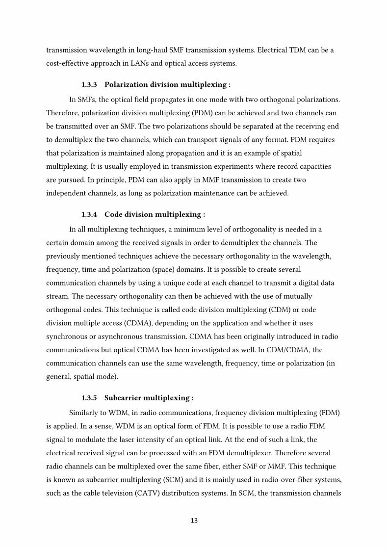
1.4.2 Presentation of optical fibers :

An optical fiber is a dielectric cylindrical waveguide. Light propagates in the core of

the optical fiber. The core is surrounded by the cladding, which has a smaller refractive

index. Therefore the mechanism of light propagation in optical fibers is total internal

reflection. The diameters of the core and the cladding, the profile of the refractive index, as

Figure 2 Multimode and single mode fibers

15

well as the material of the fiber define the type of the optical fiber and give its particular

characteristics.

An optical fiber is multimode when light propagates in more than one spatial guided

mode. A spatial guided mode, or simply a mode, can be viewed as a solution to the

electromagnetic wave propagation problem of monochromatic light in an optical fiber . It is

common not to refer to the two orthogonal polarizations of the electromagnetic field as two

different modes, but rather as the two polarizations of a mode. Alternatively, a distinct ray-

trace of light propagation in the optical fiber corresponds to a certain mode. A single mode

fiber supports only one mode in its specified wavelength operation range. Besides the

optical power that propagates along the fiber, some of the power is not bound and it is

radiated. This is usually described by the radiation modes.

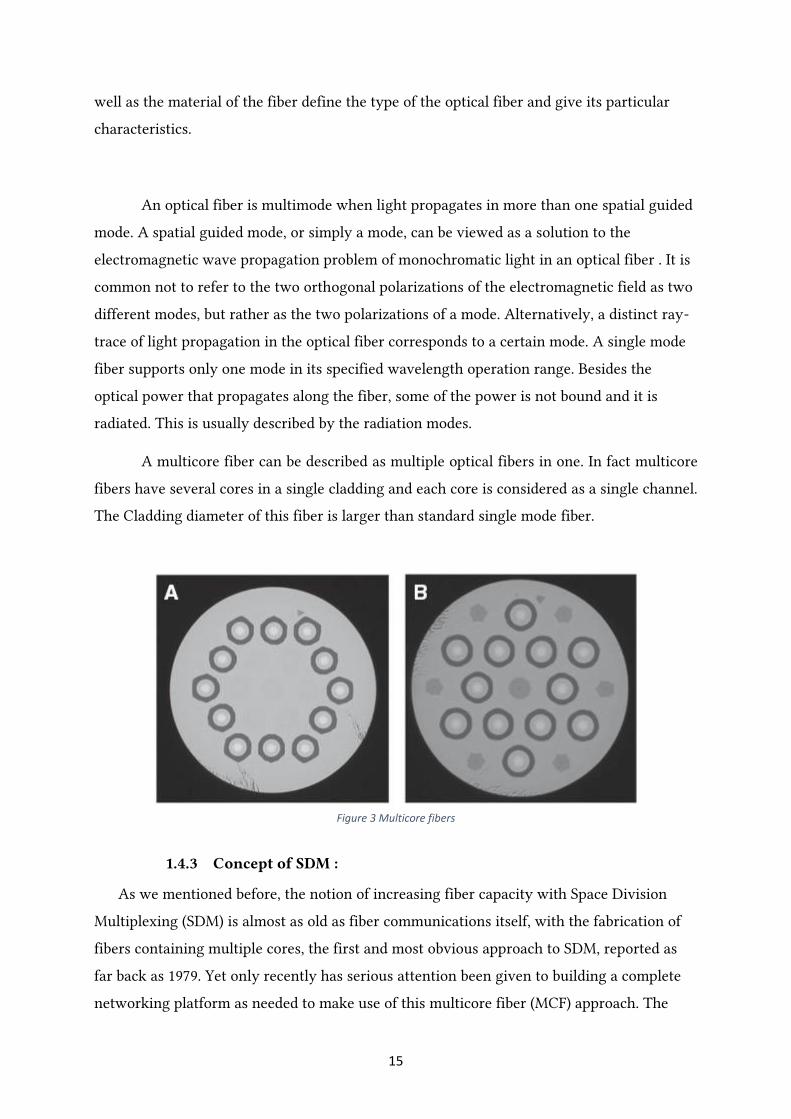
A multicore fiber can be described as multiple optical fibers in one. In fact multicore

fibers have several cores in a single cladding and each core is considered as a single channel.

The Cladding diameter of this fiber is larger than standard single mode fiber.

1.4.3 Concept of SDM :

As we mentioned before, the notion of increasing fiber capacity with Space Division

Multiplexing (SDM) is almost as old as fiber communications itself, with the fabrication of

fibers containing multiple cores, the first and most obvious approach to SDM, reported as

far back as 1979. Yet only recently has serious attention been given to building a complete

networking platform as needed to make use of this multicore fiber (MCF) approach. The

Figure 3 Multicore fibers

16

alternative approach of using modes within a multimode fiber (MMF) as a means to define

separate spatially distinct channels is called ‘Mode Division Multiplexing’ or MDM.

The current frenzied progress in SDM is occurring now because of a convergence of

enabling technological capabilities and a rapidly emerging need. On the one hand, SDM

draws on the accumulated progress of fiber research. This includes subtle improvements in

traditional fibers, and the fantastically precise fabrication methods developed to produce

hollow-core and other complex microstructure fibers. Sophisticated mode control and

analysis methods along with tapered devices can be borrowed from high-power fiber laser

research, which itself has needed to develop means to better exploit the spatial domain in

the drive to achieve ever higher power levels. These enabling technologies have made SDM

a viable strategy just as a severe need for innovation emerges.

The anticipated promise of SDM is not only that it will provide the next leap in capacity-

per-fiber, but that this will concurrently enable large reductions in cost-per-bit and

Figure 4 SDM over a few mode fiber

Figure 5 SDM over a multicore fiber

17

improved energy efficiency. This is a formidable challenge. SDM is very different from

wavelength division multiplexing (WDM) which inherently allows the sharing of key

components: e.g., an EDFA and dispersion compensation module can easily be shared by

many WDM channels with minimal added complexity. The benefits of SDM are more

speculative, and assume that many system components can be eventually integrated and

engineered to support this new platform.

1.4.4 Engineering challenges and current state :

For mode division multiplexed (MDM) transmission in MMF where the

distinguishable pathways have significant spatial overlap and, as a consequence, signals are

prone to couple randomly between the modes during propagation. In general the modes will

exhibit differential mode group delays (DMGD) and also differential modal loss or gain. The

energy of a given data symbol launched into a particular mode spreads out into adjacent

symbol time slots as a result of mode-coupling, rapidly compromising successful reception

of the information it carries. Crosstalk occurs when light is coupled from one mode to

another and remains there upon detection. Inter-symbol interference occurs when the

crosstalk is coupled back to the original mode after propagation in a mode with different

group velocity. As in wireless systems, equalization utilizing multiple-input multiple-output

(MIMO) techniques is required at the receivers to mitigate these linear impairments.

Conventional MMFs with core/cladding diameters of 50/125 and 62.5/125um support

more than 100 modes and have large DMGDs, and thus are not suitable for long-haul

transmission because the DSP complexity for MIMO equalization would be too high. Recent

advancements have led to fibers supporting a small number of modes, the so-called “few-

mode fibers” (FMFs), with low DMGD. The most significant research demonstrations have

so far concentrated on the simplest FMF, which supports three modes, the LP01 and

degenerate LP11 modes, for a total of 6 polarization and spatial modes (referred to as 3MF).

The DMGD in step-index core designs (as used in the first demonstrations of MDM in 3MF)

is a few ns/km, meaning that the number of taps required for MIMO processing was

impractical for transmission distances much greater than 10km. Consequently work has

been undertaken to develop core designs offering substantially reduced values of DMGD.

Using a graded-index (GI-) core design, DMGD values as low as 50 ps/km have been

achieved for 3MF. Moreover, it has been shown that DMGD cancellation is possible by

combining fibers fabricated to have opposite signs of DMGD. In this way transmission lines

with net values of DMGD as low as ~5ps/km (and with low levels of inherent mode-

18

coupling between mode-groups) have been realized, enabling transmission over >1000km

length scales when incorporated with an appropriate amplification approach. Whilst these

results are in themselves technically impressive, the question arises as to how scalable the

basic approach will ultimately prove. To this end, experiments have been undertaken on

both 6-mode and 5-mode FMF with encouraging initial results obtained. However, just as

with the MCF approach it is clear that scaling MDM much beyond this is likely to prove

very challenging, not least in terms of developing scalable, accurate, low-loss mode launch

schemes and ensuring that the required DSP remains tractable.

Whilst zero crosstalk would be ideal, there is a developing school of thought that

contends that mode-coupling is inevitable, that full 2Mx2M MIMO is thus necessary, and

that strong coupling should be actively exploited. If mode-coupling is weak then a data

symbol carried by multiple modes with different group indices will spread in time linearly

with fiber length. In contrast, if the coupling is strong, then the temporal spread follows a

random-walk process, and will scale with the square-root of fiber length. Strong coupling

can therefore potentially reduce the number of MIMO taps required and consequently the

DSP complexity. Indeed this is analogous to spinning of current single-mode fiber during

fabrication to reduce PMD. Similarly, the impact of differential modal gain and loss can in

principle be mitigated by strong mode-coupling over a suitable length scale relative to the

amplifier spacing.

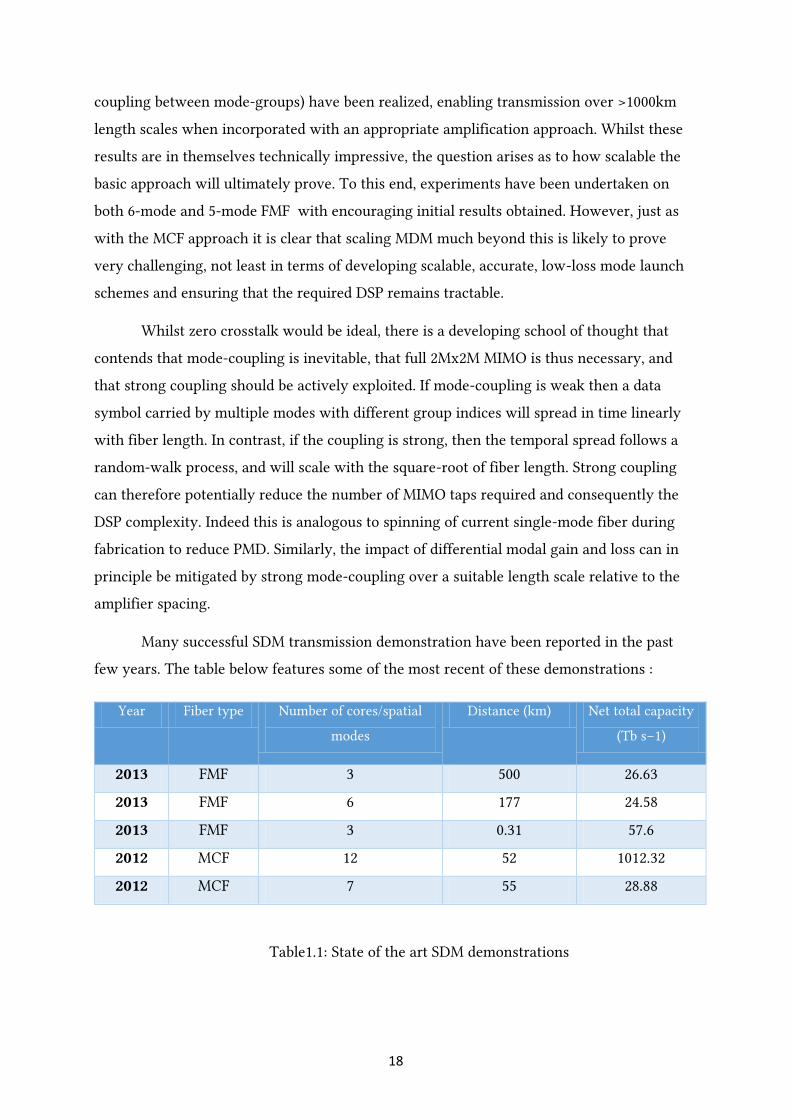
Many successful SDM transmission demonstration have been reported in the past

few years. The table below features some of the most recent of these demonstrations :

Table1.1: State of the art SDM demonstrations

Year Fiber type Number of cores/spatial

modes

Distance (km) Net total capacity

(Tb s−1)

2013 FMF 3 500 26.63

2013 FMF 6 177 24.58

2013 FMF 3 0.31 57.6

2012 MCF 12 52 1012.32

2012 MCF 7 55 28.88

19

These experiments show the feasibility of scaling capacity using SDM in FMF in combination

with MIMO signal processing.

1.5 Conclusion :

In this chapter we illustrated how the capacity of existing standard single-mode fibers is

approaching its fundamental limit regardless of significant realization of transmission

technologies which allow for high spectral efficiencies. Than we pointed out how space

division multiplexing (SDM) is currently the most promising technique of dealing with this

capacity crunch. Then we explained the concept of SDM and the engineering challenges to

overcome in order to prove it a feasible solution to the problem of saturation of the capacity

of optical transmission systems

20

2. Chapter 2 : Modes determination and optical fiber modeling

2.1 Introduction :

In this chapter we will study the propagation of light in optical fibers in order to determine

the optical modes. Then we will describe the technique we are going to use to simulate the

light propagation in optical fibers.

2.2 Optical Fiber Modes Determination :

In this chapter, we aim to describe mathematically the propagation of electromagnetic

waves in optical fibers. To do so, we will start by exposing Maxwell’s equations then we will

derive and solve the propagation equation.

2.2.1 Maxwell’s equations :

Since 1862, light was considered an electromagnetic phenomenon that can be

described accurately by the following Maxwell’s equations:

Maxwell-Gauss equation for the electric flux:

∇⃗⃗ . �⃗� = 0

Maxwell-Thomson equation for the magnetic flux:

∇⃗⃗ . �⃗⃗� =0

Maxwell-Faraday equation of magnetic induction:

∇⃗⃗ . �⃗� = −𝜇0𝜕�⃗⃗�

𝜕𝑡

Maxwell-Ampère equation for electric currents:

∇⃗⃗ × �⃗⃗� =𝜕

𝜕𝑡(휀0�⃗� + �⃗� )

Where:

�⃗� and �⃗⃗� are the electric and the magnetic fields.

(2.1)

(2.2)

(2.3)

(2.4)

21

The vector �⃗� is the induced electric polarization, which describes the response of the

medium to the electric excitation.

ε0 and µ0 are respectively the vacuum dielectric permittivity and the vacuum magnetic

permeability and are related to the light celerity in vacuum as follows : 휀0𝜇0 =1

𝑐2

2.2.2 Wave equation :

The propagation equation for an electromagnetic pulse in an optical fiber is a second

order partial differential equation that is derived directly from Maxwell’s equations.

First, we start by taking the curl of Maxwell-Faraday equation:

∇⃗⃗ × (∇⃗⃗ × �⃗� ) = −𝜇0𝜕

𝜕𝑡(∇⃗⃗ × �⃗⃗� ) = −𝜇0

𝜕²

𝜕𝑡²(휀0�⃗� + �⃗� )

Using the usual identity: ∇⃗⃗ × (∇⃗⃗ × �⃗� ) = ∇⃗⃗ (∇.⃗⃗⃗ �⃗� ) − ∇2�⃗� we get the following wave equation:

∇2�⃗� = 𝜇0휀0𝜕²�⃗�

𝜕𝑡²+휀0𝜇0휀0

𝜕²�⃗�

𝜕𝑡²

Which can be written as:

∇2�⃗� −1

𝑐2𝜕2�⃗�

𝜕𝑡2=

1

휀0𝑐²

𝜕²�⃗�

𝜕𝑡²

Generally, to identify the induced polarization rigorously, it is necessary to do some

complex quantum-mechanical analysis that will lead to the following equation:

�⃗� (𝑟 , 𝑡) = 휀0∫ 𝜒(1)(𝑡 − 𝑡′). �⃗� (𝑟 , 𝑡′)𝑑𝑡′ +∞

−∞

+ 휀0∫ ∫ 𝜒2(𝑡 − 𝑡1 , 𝑡 − 𝑡2): �⃗� +∞

−∞

+∞

−∞

(𝑟 , 𝑡1)�⃗� (𝑟 , 𝑡2)𝑑𝑡1𝑑𝑡2

+ ∫ ∫ ∫ 𝜒3(𝑡 − 𝑡1 , 𝑡 − 𝑡2, 𝑡 − 𝑡3) ⋮ �⃗� (𝑟 , 𝑡1)�⃗� (𝑟 , 𝑡2)�⃗� (𝑟 , 𝑡3)𝑑𝑡1𝑑𝑡2𝑑𝑡3 +∞

−∞

+∞

−∞

+∞

−∞

+⋯

(2.5)

(2.6)

22

where 𝜒𝑗 is the so-called jth order susceptibility represented by a tensor of rank j+1.

Obviously, this formula can lead to an enormous complexity. Hence, it is necessary to simplify

it as much as possible without neglecting any important physical effects.

First of all, in optical telecommunications, terms of order higher than three have no

considerable impact on our study.

Furthermore, thanks to the symmetry of silica glass molecules SiO2, 𝜒(2) vanishes.

This leaves us to consider only the 1st order term of susceptibility which is responsible

for the linear effects and the 3rd order susceptibility accounting for non- linear effects.

Thus, the polarization vector can be separated into a linear term and a non-linear term

as written below:

�⃗� = �⃗� 𝐿 + �⃗� 𝑁𝐿

Where the linear polarization �⃗� 𝐿 is given by the relation :

�⃗� 𝐿 = 휀0∫ 𝜒1(𝑡 − 𝑡′). �⃗� (𝑟 , 𝑡′)𝑑𝑡′+∞

−∞

And the non-linear polarization �⃗� 𝑁𝐿 is given by:

�⃗� 𝑁𝐿 = 휀0∫ ∫ ∫ 𝜒3(𝑡 − 𝑡1, 𝑡 − 𝑡2, 𝑡 − 𝑡3): �⃗� (𝑟 , 𝑡1)�⃗� (𝑟 , 𝑡2)𝑑𝑡1𝑑𝑡2 +∞

−∞

+∞

−∞

+∞

−∞

Because of the high complexity, it is necessary to make more simplifying

approximations. Therefore, the nonlinear polarization is treated as a small perturbation to the

total induced polarization i.e : �⃗� 𝑁𝐿 = 0⃗ . It is also useful to work in the frequency domain:

∇2Ẽ + 휀0(𝜔)𝜔2

𝑐2Ẽ = 0

where Ẽ(r,ω) is the fourier transform of E(r,t) defined as:

𝐸(𝑟, 𝑡) =1

2𝜋∫ Ẽ(𝑟, 𝜔) exp(−𝑖𝜔𝑡) 𝑑𝜔+∞

−∞

At this level, we define the frequency-dependent dielectric constant 휀(𝜔) as follows:

휀(𝜔) = 1 + 𝜒(1)(𝜔)

(2.8)

(2.9)

(2.10)

1

(2.11)

(2.12)

23

where 𝜒(1)(𝜔) stands for the Fourier transform of χ(1).

Note that generally, 𝜒1(𝜔) is complex, so the frequency dependent dielectric constant

is also a complex number. This number can be used to determine the refractive index 𝑛 and

the absorption given by a coefficient 𝛼 using this formula :

휀 = (𝑛 +𝑖𝛼𝑐

2𝜔)2

Therefore, we can deduce explicitly the expressions of 𝑛 and 𝛼:

𝑛(𝜔) = 1 +1

2𝑅𝑒[𝜒~(1) (𝜔)]

𝛼(𝜔) =𝜔

𝑛𝑐𝑙𝐼𝑚[𝜒~(1)(𝜔)]

The imaginary part of ε is small in comparison to the real part. Thus, we can replace ε

by 𝑛2(𝜔).

Finally, we can write the wave equation in the frequency domain as:

∇2Ẽ + 𝑛2𝜔2

𝑐2Ẽ = 0

We can now define the wave number as follows:

𝑘0 =𝜔

𝑐=2𝜋

𝜆

Hence, the wave equation becomes:

∇2Ẽ + 𝑛2𝑘02Ẽ = 0

Which has the form of a well-known equation called the Helmholtz equation.

2.2.3 Bessel Equation :

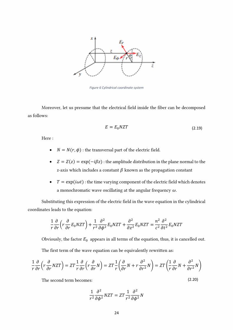
Since the geometry of the fiber is cylindrical, it is more convenient to continue our

study in the cylindrical frame of reference (see figure 1.1) characterized by the following

spatial coordinates(𝑟, 𝜙, 𝑧).

(2.13)

(2.14)

(2.15)

(2.16)

(2.17)

(2.18)

24

Moreover, let us presume that the electrical field inside the fiber can be decomposed

as follows:

𝐸 = 𝐸0𝑁𝑍𝑇

Here :

𝑁 = 𝑁(𝑟, 𝜙) : the transversal part of the electric field.

𝑍 = 𝑍(𝑧) = exp (−𝑖𝛽𝑧) : the amplitude distribution in the plane normal to the

z-axis which includes a constant 𝛽 known as the propagation constant

𝑇 = exp (𝑖𝜔𝑡) : the time varying component of the electric field which denotes

a monochromatic wave oscillating at the angular frequency 𝜔.

Substituting this expression of the electric field in the wave equation in the cylindrical

coordinates leads to the equation:

1

𝑟

𝜕

𝜕𝑟(𝑟𝜕

𝜕𝑟𝐸0𝑁𝑍𝑇) +

1

𝑟2𝜕2

𝜕𝜙2𝐸0𝑁𝑍𝑇 +

𝜕2

𝜕𝑧2𝐸0𝑁𝑍𝑇 =

𝑛2

𝑐2𝜕2

𝜕𝑡2𝐸0𝑁𝑍𝑇

Obviously, the factor 𝐸0 appears in all terms of the equation, thus, it is cancelled out.

The first term of the wave equation can be equivalently rewritten as:

1

𝑟

𝜕

𝜕𝑟(𝑟𝜕

𝜕𝑟𝑁𝑍𝑇) = 𝑍𝑇

1

𝑟

𝜕

𝜕𝑟(𝑟𝜕

𝜕𝑟𝑁) = 𝑍𝑇

1

𝑟(𝜕

𝜕𝑟𝑁 + 𝑟

𝜕2

𝜕𝑟2𝑁) = 𝑍𝑇 (

1

𝑟

𝜕

𝜕𝑟𝑁 +

𝜕2

𝜕𝑟2𝑁)

The second term becomes:

1

𝑟2𝜕2

𝜕𝜙2𝑁𝑍𝑇 = 𝑍𝑇

1

𝑟2𝜕2

𝜕𝜙2𝑁

(2.19)

(2.20)

Figure 6 Cylindrical coordinate system

25

and the third:

𝜕2

𝜕𝑧2𝑁𝑍𝑇 = 𝑁𝑇

𝜕2

𝜕𝑧2𝑍 = −𝛽2𝑁𝑍𝑇

On the right hand side:

𝑛2

𝑐2𝜕2

𝜕𝑡2𝑁𝑍𝑇 = 𝑁𝑍

𝑛2

𝑐2𝜕2

𝜕𝑡2𝑇 = −𝑁𝑍𝑇𝜔2

𝑛2

𝑐2= −𝑛2𝑘0

2𝑁𝑍𝑇

We notice now, that the factor ZT is common to all terms, so this factor is also

cancelled out.

Therefore, the wave equation becomes:

(1

𝑟

𝜕

𝜕𝑟𝑁 +

𝜕2

𝜕𝑟2𝑁) +

1

𝑟2𝜕2

𝜕𝜙2𝑁 − 𝛽2𝑁 = −𝑛2𝑘0

2𝑁

We are left with an equation of the amplitude distribution of the electric field in the

plane normal to the propagation direction. To resolve this equation, we have to make a further

factorization: 𝑁(𝑟, 𝜙) = 𝑅(𝑟)Φ(𝜙)

Substituting this expression in the wave equation and multiplying all terms by 𝑟2

𝑅Φ and

then rearranging all terms leads to the equation below:

−1

Φ

𝜕2

𝜕𝜙2Φ =

1

𝑅 (𝑟2

𝜕2

𝜕𝑟2𝑅 + 𝑟

𝜕

𝜕𝑟𝑅 + 𝑟2(𝑘2 − 𝛽2)𝑅

We see that the right hand side depends only on R whereas the left hand side depends

only on Φ. Therefore, both sides must be equal to a constant which we presume positive and

we will denote it 𝑚2 .

These assumptions leave us with two independent equations of the form:

1

Φ

𝜕2

𝜕𝜙2Φ+m2 = 0

1

𝑅 (𝑟2

𝜕2

𝜕𝑟2𝑅 + 𝑟

𝜕

𝜕𝑟𝑅 + 𝑟2(𝑘2 − 𝛽2)𝑅 = 𝑚2

×𝑅⇔ 𝑟2

𝜕2

𝜕𝑟2𝑅 + 𝑟

𝜕

𝜕𝑟𝑅 + 𝑅[(𝑘2 − 𝛽2)𝑟2 −𝑚2] = 0

By using the abbreviation: 𝜅2 = 𝑘02 − 𝛽2, the equation above becomes :

(2.21)

(2.22)

(2.23)

(2.24)

(2.25)

(2.26)

26

𝑟2𝜕2

𝜕𝑟2𝑅 + 𝑟

𝜕

𝜕𝑟𝑅 + 𝑅(𝜅2𝑟2 −𝑚2) = 0

Before moving to the mode analysis and resolving the two equations above, it is

necessary to discuss the meaning of the constants 𝑘, 𝜅, 𝑎𝑛𝑑 𝛽.

To do so, all we need is the ray-optical description where the rays make small angles

with the axes.

In this approach, k stands for the wave number as mentioned before.

𝛽 : the propagation constant, can be seen as the component of the wave number k in

the propagation direction.

Finally, 𝜅 can be understood as the transverse component of the wave number k.

Note here, that all these assumptions are deduced directly from the equation:

𝜅2 = 𝑘02 − 𝛽2 which can be written in an equivalent way as: 𝑘0

2 = 𝛽2 + 𝜅2 which

stands for the Pythagorean identity.

The equation :

1

Φ

𝜕2

𝜕𝜙2Φ+m2 = 0

has the general solution :

Φ(𝑚) = 𝑐0 cos(𝑚𝜙 + 𝜙0)

Where 𝑐0 and 𝜙0 are constants. Surely, Φ(𝑚) and 𝜕Φ

𝜕𝜙 must be continuous at

𝜙 = 0 𝑎𝑛𝑑 𝜙 = 2𝜋 which leads to:

Φ(0) = 𝑐0 cos(𝜙0) = Φ(2𝜋) = 𝑐0cos (2𝑚𝜋 + 𝜙0)

This relation suggests that m must be an integer.

The radial equation:

(2.27)

(2.29)

27

𝑟2𝜕2

𝜕𝑟2𝑅 + 𝑟

𝜕

𝜕𝑟𝑅 + 𝑅(𝜅2𝑟2 −𝑚2) = 0

is of the form:

𝑥2𝑦′′ + 𝑥𝑦′ + (𝜅2𝑥2 −𝑚2)𝑦 = 0

Which stands for a standard Bessel equation. For m integer, the solutions are of the

form:

𝑦(𝑥) = 𝑐1𝐽𝑚(𝜅𝑥) + 𝑐2𝑁𝑚(𝜅𝑥)

Or, in the other form:

𝑦(𝑥) = 𝑐3𝐼𝑚(𝜅𝑥) + 𝑐4𝐾𝑚(𝜅𝑥)

Where: 𝐽𝑚 and 𝑁𝑚 are special functions called Bessel functions.

This type of functions has an oscillatory behavior. Thus, it’s convenient to describe

the propagation inside the core regions. That is why, we are going to consider those functions

whenever the condition: 𝑟 ≤ 𝑎 is satisfied (a stands here for the core radius).

However, 𝐼𝑚 and 𝐾𝑚 are a non-oscillatory Bessel functions that are more convenient

to describe the wave behavior in the cladding region. So, we are going to use these functions

whenever the condition 𝑟 ≥ 𝑎 is satisfied.

2.2.4 Mode determination:

Considering that the solution has to be smoothly continuous on the boundaries, which

means that 𝑅(𝑟) and 𝜕

𝜕𝑟𝑅 are continuous, and the fact that the field amplitude is inversely

proportional to the distance r, we are left with the following condition:

𝐽𝑚(𝑢)

𝑢𝐽𝑚+1(𝑢)=

𝐾𝑚(𝑤)

𝑤𝐾𝑚+1(𝑤)

Where 𝑢 = 𝜅𝑐𝑜𝑎 and 𝑘𝑐𝑜2 = 𝑛𝑐𝑜2 𝑘02 − 𝛽2 is the transverse component of the wave

number inside the core and 𝑤 = 𝜅𝑐𝑙𝑎 and 𝜅𝑐𝑙2 = 𝛽2 − 𝑛𝑐𝑙

2 𝑘02 is the transverse component

inside the cladding region.

Note here that:

(2.30)

(2.31)

(2.32)

(2.33)

28

𝑢2 + 𝑤2 = (𝜅𝑐𝑜2 + 𝜅𝑐𝑙

2 )𝑎2 = 𝑎2(𝑛𝑐𝑜2 𝑘0

2 − 𝛽2 + 𝛽2 − 𝑛𝑐𝑙2 𝑘0

2) = 𝑎2𝑘02(𝑛𝑐𝑜

2 − 𝑛𝑐𝑙2 )

The quantity: √𝑎2𝑘02(𝑛𝑐𝑜2 − 𝑛𝑐𝑙

2 ) = 𝑎𝑘0√(𝑛𝑐𝑜2 − 𝑛𝑐𝑙2 ) is denoted V and called the

normalized frequency.

This constant is of central importance because it resumes all the properties of the

optical fibers. In fact, it includes the geometry of the fiber which is represented by the factor

a, it includes also the chemical properties of the materials which are represented by the

refractive indices of the core and the cladding regions and finally it contains the injected

wavelength which reveals the physical aspect.

The V number can reveal the number of the supported modes when using some well-

known approximation relations.

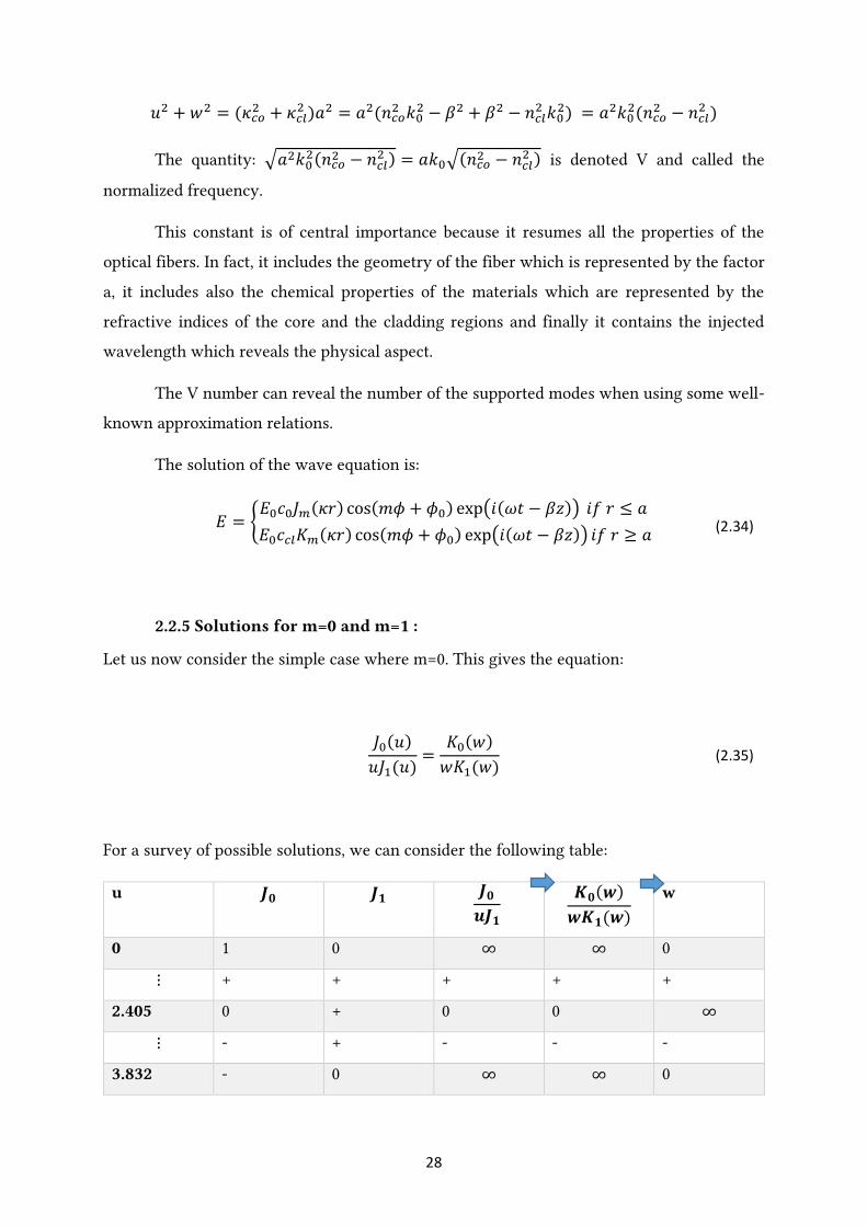
The solution of the wave equation is:

𝐸 = {𝐸0𝑐0𝐽𝑚(𝜅𝑟) cos(𝑚𝜙 + 𝜙0) exp(𝑖(𝜔𝑡 − 𝛽𝑧)) 𝑖𝑓 𝑟 ≤ 𝑎

𝐸0𝑐𝑐𝑙𝐾𝑚(𝜅𝑟) cos(𝑚𝜙 + 𝜙0) exp(𝑖(𝜔𝑡 − 𝛽𝑧)) 𝑖𝑓 𝑟 ≥ 𝑎

2.2.5 Solutions for m=0 and m=1 :

Let us now consider the simple case where m=0. This gives the equation:

𝐽0(𝑢)

𝑢𝐽1(𝑢)=𝐾0(𝑤)

𝑤𝐾1(𝑤)

For a survey of possible solutions, we can consider the following table:

u 𝑱𝟎 𝑱𝟏 𝑱𝟎𝒖𝑱𝟏

𝑲𝟎(𝒘)

𝒘𝑲𝟏(𝒘)

w

0 1 0 ∞ ∞ 0

⋮ + + + + +

2.405 0 + 0 0 ∞

⋮ - + - - -

3.832 - 0 ∞ ∞ 0

(2.34)

(2.35)

29

⋮ - - + + +

5.520 0 - 0 0 ∞

⋮ + - - - -

Table 2.1: Determination of possible solutions

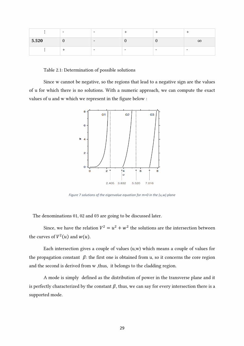
Since w cannot be negative, so the regions that lead to a negative sign are the values

of u for which there is no solutions. With a numeric approach, we can compute the exact

values of u and w which we represent in the figure below :

Figure 7 solutions of the eigenvalue equation for m=0 in the (u,w) plane

The denominations 01, 02 and 03 are going to be discussed later.

Since, we have the relation 𝑉2 = 𝑢2 + 𝑤2 the solutions are the intersection between

the curves of 𝑉2(𝑢) and 𝑤(𝑢).

Each intersection gives a couple of values (u,w) which means a couple of values for

the propagation constant 𝛽: the first one is obtained from u, so it concerns the core region

and the second is derived from w ,thus, it belongs to the cladding region.

A mode is simply defined as the distribution of power in the transverse plane and it

is perfectly characterized by the constant 𝛽, thus, we can say for every intersection there is a

supported mode.

30

We also notice from the figure above that the particular value: V=2.405 marks the

transition of a unique solution to more than one solution. So, below this value, the fiber can

support only one mode and it is called single mode fiber.

Above this value, many modes are supported and the fiber is then called multimode fiber.

We can notice also that at higher wavelengths, V is always below 2.405, so the fiber is

obviously a single mode fiber. This implies that the qualifications single mode or multimode

have meaning only in relation to a specific wavelength.

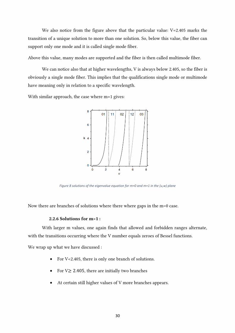
With similar approach, the case where m=1 gives:

Figure 8 solutions of the eigenvalue equation for m=0 and m=1 in the (u,w) plane

Now there are branches of solutions where there where gaps in the m=0 case.

2.2.6 Solutions for m>1 :

With larger m values, one again finds that allowed and forbidden ranges alternate,

with the transitions occurring where the V number equals zeroes of Bessel functions.

We wrap up what we have discussed :

For V<2.405, there is only one branch of solutions.

For V≥ 2.405, there are initially two branches

At certain still higher values of V more branches appears.

31

2.2.7 Field amplitude distribution of the modes:

To complete our analysis, we are going to plot the expression of E and for convenience

the radial and the azimuthal terms will be plotted separately.

The field E is given by:

𝐸 = {𝐸0𝑐0𝐽𝑚(𝜅𝑟) cos(𝑚𝜙 + 𝜙0) exp(𝑖(𝜔𝑡 − 𝛽𝑧)) 𝑖𝑓 𝑟 ≤ 𝑎

𝐸0𝑐𝑐𝑙𝐾𝑚(𝜅𝑟) cos(𝑚𝜙 + 𝜙0) exp(𝑖(𝜔𝑡 − 𝛽𝑧)) 𝑖𝑓 𝑟 ≥ 𝑎

We now see that the modes form a two-parameter family. The first parameter is m. m

indicates as shown in the formula above the angular dependency of the field distribution of

the mode.

For m=0: the distribution is rotationally invariant ie: on any circular path at a given r

one would find a constant field amplitude and thus intensity.

For m=1: the field amplitude will vary according to a sine function of the azimuthal

angle. It therefore, has two zeroes at opposite positions. In between, there are a positive and

a negative branch, or lobe. Either branch contains the maximum of the intensity while the

algebraic sign indicates the phase of the field. Thus, in one lobe the field oscillates in opposite

phase to the other.

For m=2: a circular path would run through two full periods of the sine function; the

intensity pattern then resembles a four-leaved clover. Again, each one of the leaves in

opposite positions has the same phase while the other has the opposite phase.

When m takes even higher values, the angular dependency of the field amplitude has

2m leaves.

The parameter m fixes also which Bessel function governs the field distribution in the

radial direction: we have found a combination of Jm in the core and Km in the cladding.

Since Jm oscillates at any m, there are infinitely many ways to smoothly connect Jm to

Km even after m has been fixed. This set of possibilities is labeled with p, the second

parameter.

We adopt here the terminology of modes as introduced in 1971 by Gloge: modes are

designated with 𝐿𝑃𝑚𝑝 on grounds that they are essentially linearly polarized. Index m

designates the number of pairs of nodes in the azimuthal coordinate, and index p counts the

possibilities in the radial coordinate.

32

This explanation can be visualized through the following figures:

Figure 9 Field intensity distribution for m=0

Figure 10 Field intensity distribution for m=1 Figure 11 Field intensity distribution for m=2

33

2.2.8 Analogy with microwave waveguides:

Microwave waveguides are metal pipes with conducting walls. This enforces a node

of the electrical field on the boundary.

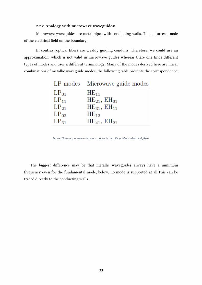
In contrast optical fibers are weakly guiding conduits. Therefore, we could use an

approximation, which is not valid in microwave guides whereas there one finds different

types of modes and uses a different terminology. Many of the modes derived here are linear

combinations of metallic waveguide modes, the following table presents the correspondence:

Figure 12 correspondence between modes in metallic guides and optical fibers

The biggest difference may be that metallic waveguides always have a minimum

frequency even for the fundamental mode; below, no mode is supported at all.This can be

traced directly to the conducting walls.

34

2.3 Modeling the optical fiber :

For our modeling purposes we are going to perform a finite element analysis using a FEM

software.

the finite element method (FEM) is a numerical technique for finding approximate solutions

to boundary value problems for differential equations. It uses variational methods to minimize

an error function and produce a stable solution. Analogous to the idea that connecting many

tiny straight lines can approximate a larger circle, FEM encompasses all the methods for

connecting many simple element equations over many small subdomains, named finite

elements, to approximate a more complex equation over a larger domain.

Figure 13 Dividing a sphere into smaller finite elements (meshing) progressively

Figure 14 Different types of finite elements that can be used in meshing

35

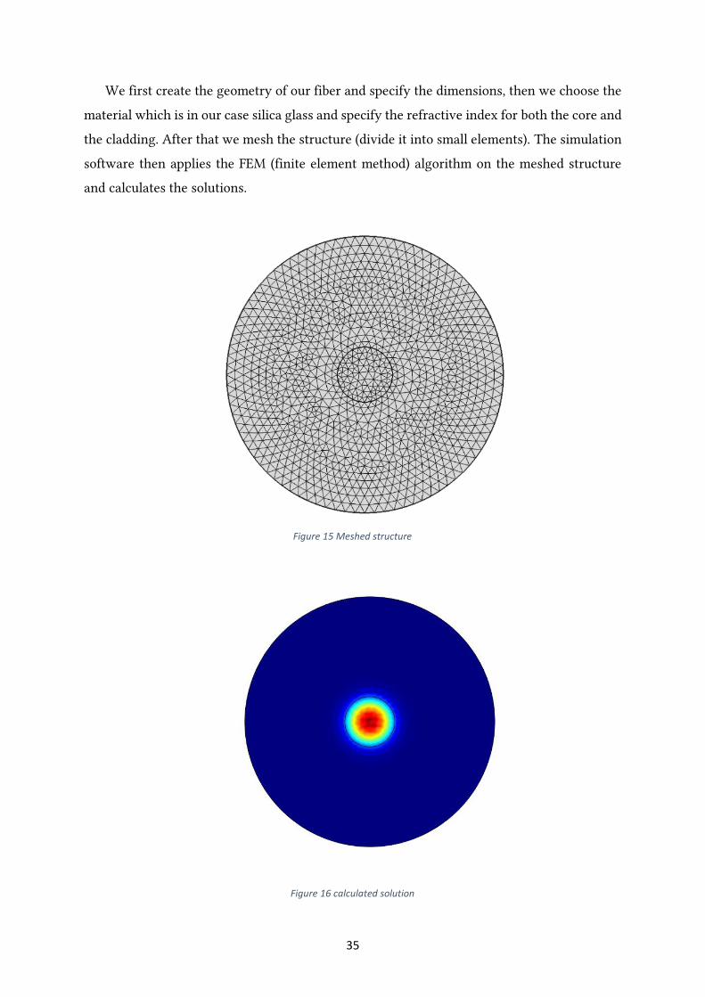
We first create the geometry of our fiber and specify the dimensions, then we choose the

material which is in our case silica glass and specify the refractive index for both the core and

the cladding. After that we mesh the structure (divide it into small elements). The simulation

software then applies the FEM (finite element method) algorithm on the meshed structure

and calculates the solutions.

Figure 15 Meshed structure

Figure 16 calculated solution

36

2.4 Conclusion :

In this chapter we demonstrated mathematically and in detail how to determine the optical

modes in the fiber based on maxwell’s equations and the weakly guided modes

approximation. Then we explained how to model the optical fiber using a finite element

analysis software to solve numerically the differential equations describing the light

propagation in the fiber and thus obtain the values of the field distribution of each mode in

the fiber.

37

3. Chapter 3 : Study of key system performance parameters in a MDM transmission system

3.1 Introduction :

After successfully modeling the fiber as described in chapter 2, in this chapter we will

carry out a parametric study on the propagation of the modes in the fiber to evaluate the

influence of each parameter on mode coupling which is the main obstacle for MDM

transmission that limits the performance and reach of MDM systems.

3.2 Definition and perspective :

The concept of mode coupling is very often used e.g. to describe the propagation of

light in some waveguides or optical cavities under the influence of additional effects, such as

external disturbances or nonlinear interactions. The basic idea of coupled-mode theory is to

decompose all propagating light into the known modes of the undisturbed device, and then

to calculate how these modes are coupled with each other by some additional influence. This

approach is often technically and conceptually much more convenient than, e.g., recalculating

the propagation modes for the actual situation in which light propagates in the device [1].

Some examples of mode coupling are discussed in the following:

• An optical fiber may have several propagation modes, to be calculated for the fiber being

kept straight. If the fiber is strongly bent, this can introduce coupling e.g. from the

fundamental mode to higher-order propagation modes (even to cladding modes), or coupling

between different polarization states. Bend losses can be understood as coupling to non-

guided (and thus lossy) modes.

• Nonlinear interactions in a waveguide can also couple the modes (as calculated for low light

intensities) to each other. This picture can serve e.g. to describe processes such as frequency

doubling in a waveguide, where the nonlinear coupling mechanism transfers amplitude (and

optical power) from the pumped mode into a mode with twice the optical frequency.

• In high-power fiber amplifiers, a mechanism has been identified which can couple power

from the fundamental fiber mode into higher-order modes . This mechanism can involve

38

either a Kramers–Kronig effect or thermal distortions influencing the refractive index profile.

This leads to a strong loss of beam quality above a certain pump power level.

Technically, the mode coupling approach is often used in the form of coupled

differential equations for the complex excitation amplitudes of all the involved modes. These

equations contain coupling coefficients, which are usually calculated from overlap integrals,

involving the two mode functions and the disturbance causing the coupling. Typically, the

applied procedure is first to calculate the mode amplitudes for the given light input, then to

propagate these amplitudes based on the above-mentioned coupled differential equations (e.g.

using some Runge–Kutta algorithm), and finally (if required) to recombine the mode fields to

obtain the resulting field distribution.

An important physical aspect of such coherent mode coupling phenomena is that the

optical power transferred between two modes depends on the amplitudes which are already

in both modes. A consequence of that is that the power transfer from a mode A to another

mode B can be kept very small simply by strongly attenuating mode B. In this way, mode B

is prevented from acquiring sufficient power to extract power from mode A efficiently, so

that mode A experiences only little loss, despite the coupling.

3.3 Mode coupling and its origins :

In an ideal fiber, modes propagate without cross-coupling. In a real fiber,

perturbations, whether intended or unintended, can induce coupling between spatial and/or

polarization modes. Throughout this chapter, we consider only coupling between forward-

propagating modes, since it has a dominant effect on the system properties of interest,

including MD and MDL. In multimode transmission fibers, unintended mode coupling can

arise from several sources. These include manufacturing variations causing non-circularity of

the core, roughness at the core-cladding boundary, variations in the core radius, or variations

in the index profile in graded-index fibers. They also include stresses induced by the jacket,

or by thermal mismatches between glasses of different compositions. Finally, mode coupling

can arise from micro-bending, macro-bending, or twists [2].

3.4 Coupled power theory :

In his book ‘theory of dielectric optical waveguide’ , D.Marcuse presented an

exact coupled mode theory that is capable, at least in principle, of handling any kind of mode

conversion and radiation effect that may occur in a multimode or single-mode optical

dielectric waveguide. However, the infinite set of coupled integro-differential equations

39

obtained is very hard to solve. In addition, the problem of a randomly deformed multimode

waveguide is too complex to be treated directly with the coupled wave theory. The complexity

of the coupled wave equations is caused by the fact that they contain too much information.

The system of coupled equations contains a detailed description of the phase and amplitude

of all the modes at any point along the waveguide. However, as this report represents a first

approach to studying mode coupling in fibers we will try to use a simpler model.

For many practical purposes, especially MMF systems using spatially and temporally

incoherent light emitting diodes, it would suffice to know the average amount of power

carried by each mode or groups of modes. We are interested to know how the total power

carried by the waveguide is distributed among the modes and how this distribution is

changing as a result of coupling and loss processes.

The coupled power equations hold only for relatively weak coupling. However, this

weak coupling case is most often encountered in practical applications. Weak coupling means

that changes in the power distribution take place over distances that are very long compared

to the wavelength of light. Undesired, random coupling caused by waveguide imperfections

is always weak and is thus accessible to the approximate coupled power theory. This approach

is also suitable for geometrical perturbations, such as bends or tapers, which represent large

deviations from an ideal fiber, provided they vary slowly along the fiber’s length [2,4].

In the simple case of two modes, the power coupling equations [5,ch.5] are :

𝑑𝑃1𝑑𝑧

= −𝛼𝑃1 + ℎ12(𝑃2 − 𝑃1)

𝑑𝑃2𝑑𝑧

= −𝛼𝑃2 + ℎ12(𝑃1 − 𝑃2)

With the initial conditions : P1(0)=P01 and P2(0)=P02.

where we have assumed equal attenuation coefficients for the two modes (α).

h12: is the intermodal coupling coefficient which measures the probability per unit length of

a transition occurring between modes 1 and 2.

Note that h12 is symmetric which means h12=h21.

(3.1)

(3.2)

40

On the right-hand side, the first term describes loss by power attenuation coefficient

α, and the second term describes coupling by non-negative real coefficient h12 [2,ch.11 ;

4,ch.12].

ℎ12 = ⟨|∫ 𝐶12(𝑧)𝑒−𝑗(𝛽1−𝛽2)𝑧𝑑𝑧

𝐿

0

|

2

⟩

𝐶12 =𝜔휀04∫ ∫ 𝛿𝑛2(𝑥, 𝑦)𝐸1

∗(𝑥, 𝑦)𝐸2(𝑥, 𝑦)𝑑𝑥𝑑𝑦 +∞

−∞

+∞

−∞

Assuming a perturbed index profile of the form :

n2(x, y, z) = n02(x, y) + δn2(x, y)*f(z)

(3.2) → 𝑃1 =1

ℎ12(𝑑𝑃2𝑑𝑧

+ (𝛼 + ℎ12)𝑃2)

𝑡ℎ𝑒𝑛 𝑖𝑓 𝑤𝑒 𝑖𝑛𝑗𝑒𝑐𝑡 (3.6) 𝑖𝑛 (3.1) 𝑤𝑒 𝑔𝑒𝑡 ∶

𝑑2𝑃2𝑑𝑧2

+ 2(𝛼 + ℎ12)𝑑𝑃2𝑑𝑧

+ (𝛼2 + 2𝛼ℎ12)𝑃2 = 0

To solve this second order differential equation we have to solve the characteristic

equation first :

𝑚2 + 2(𝛼 + ℎ12)𝑚 + (𝛼2 + 2𝛼ℎ12) = 0

The solutions for this second order equation are :

𝑚1 = −𝛼 𝑎𝑛𝑑 𝑚2 = −𝛼 − 2ℎ12

which means the general solution for P2 is :

𝑃2(𝑧) = 𝐶1𝑒−𝛼𝑧 + 𝐶2𝑒

(−𝛼−2ℎ12)𝑧

finally , considering the initial conditions we get :

𝑃2(𝑧) =(𝑃01 + 𝑃02)

2𝑒−𝛼𝑧 +

(𝑃02 − 𝑃01)

2𝑒−(𝛼+2ℎ12)𝑧

Similarly :

𝑃1(𝑧) =(𝑃01 + 𝑃02)

2𝑒−𝛼𝑧 +

(𝑃01 − 𝑃02)

2𝑒−(𝛼+2ℎ12)𝑧

(3.3)

(3.4)

(3.5)

(3.6)

(3.7)

(3.8)

(3.9)

(3.10)

(3.11)

(3.12)

41

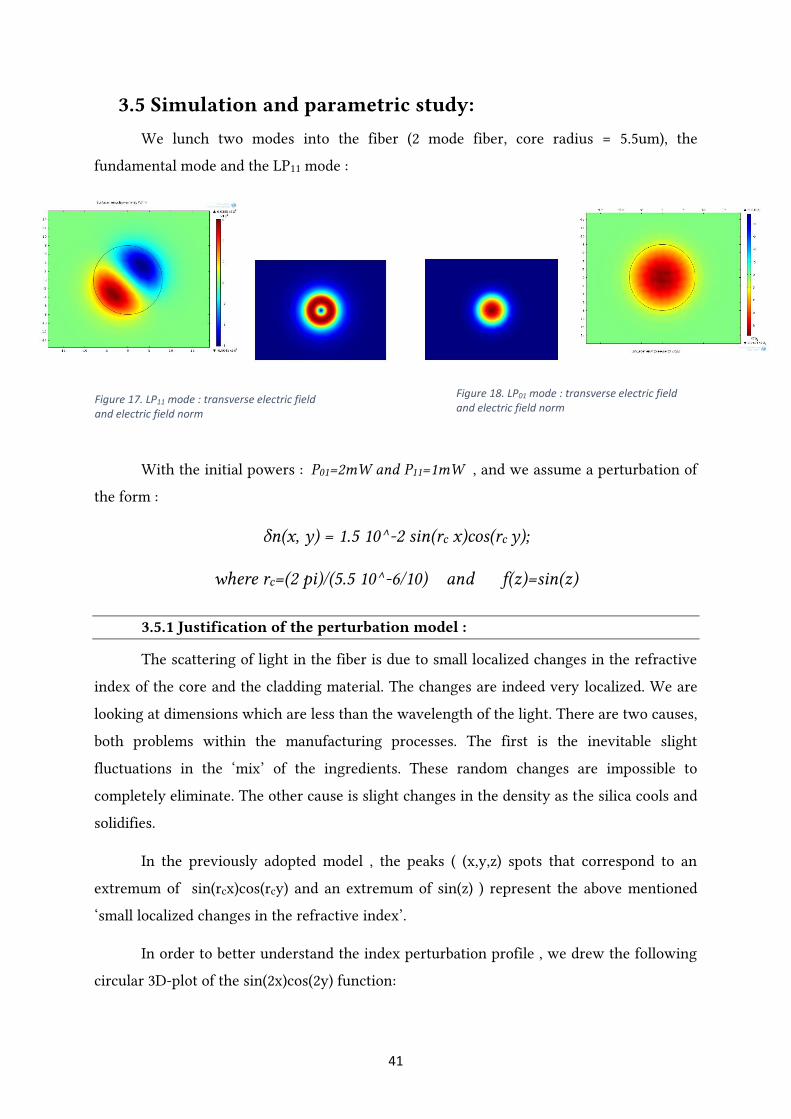
3.5 Simulation and parametric study:

We lunch two modes into the fiber (2 mode fiber, core radius = 5.5um), the

fundamental mode and the LP11 mode :

With the initial powers : P01=2mW and P11=1mW , and we assume a perturbation of

the form :

δn(x, y) = 1.5 10^-2 sin(rc x)cos(rc y);

where rc=(2 pi)/(5.5 10^-6/10) and f(z)=sin(z)

3.5.1 Justification of the perturbation model :

The scattering of light in the fiber is due to small localized changes in the refractive

index of the core and the cladding material. The changes are indeed very localized. We are

looking at dimensions which are less than the wavelength of the light. There are two causes,

both problems within the manufacturing processes. The first is the inevitable slight

fluctuations in the ‘mix’ of the ingredients. These random changes are impossible to

completely eliminate. The other cause is slight changes in the density as the silica cools and

solidifies.

In the previously adopted model , the peaks ( (x,y,z) spots that correspond to an

extremum of sin(rcx)cos(rcy) and an extremum of sin(z) ) represent the above mentioned

‘small localized changes in the refractive index’.

In order to better understand the index perturbation profile , we drew the following

circular 3D-plot of the sin(2x)cos(2y) function:

Figure 17. LP11 mode : transverse electric field and electric field norm

Figure 18. LP01 mode : transverse electric field and electric field norm

42

The following figure illustrates the evolution of the refractive index of the fiber along

the z axis (which is periodic since f(z)=sin(z)) :

Figure 19 3D plot of the sin(2x)*cos(2y) function

Figure 20 Evolution of the perturbed refractive index as a function of the distance z

43

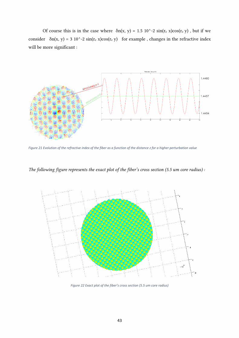
Of course this is in the case where δn(x, y) = 1.5 10^-2 sin(rc x)cos(rc y) , but if we

consider δn(x, y) = 3 10^-2 sin(rc x)cos(rc y) for example , changes in the refractive index

will be more significant :

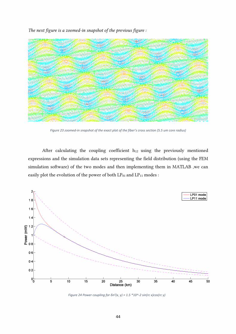
The following figure represents the exact plot of the fiber’s cross section (5.5 um core radius) :

Figure 22 Exact plot of the fiber’s cross section (5.5 um core radius)

Figure 21 Evolution of the refractive index of the fiber as a function of the distance z for a higher perturbation value

44

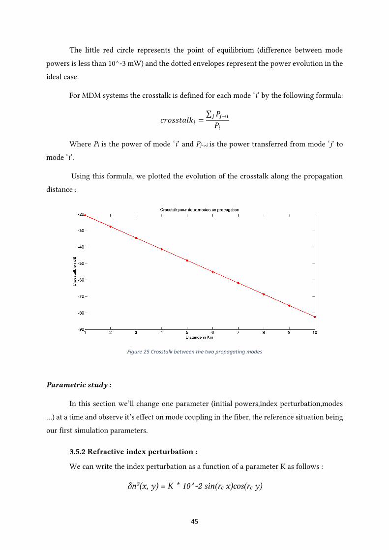
The next figure is a zoomed-in snapshot of the previous figure :

Figure 23 zoomed-in snapshot of the exact plot of the fiber’s cross section (5.5 um core radius)

After calculating the coupling coefficient h12 using the previously mentioned

expressions and the simulation data sets representing the field distribution (using the FEM

simulation software) of the two modes and then implementing them in MATLAB ,we can

easily plot the evolution of the power of both LP01 and LP11 modes :

Figure 24 Power coupling for δn2(x, y) = 1.5 *10^-2 sin(rc x)cos(rc y)

45

The little red circle represents the point of equilibrium (difference between mode

powers is less than 10^-3 mW) and the dotted envelopes represent the power evolution in the

ideal case.

For MDM systems the crosstalk is defined for each mode ‘i’ by the following formula:

𝑐𝑟𝑜𝑠𝑠𝑡𝑎𝑙𝑘𝑖 =∑ 𝑃𝑗→𝑖𝑗

𝑃𝑖

Where Pi is the power of mode ‘i’ and Pj->i is the power transferred from mode ‘j’ to

mode ‘i’.

Using this formula, we plotted the evolution of the crosstalk along the propagation

distance :

Parametric study :

In this section we’ll change one parameter (initial powers,index perturbation,modes

…) at a time and observe it’s effect on mode coupling in the fiber, the reference situation being

our first simulation parameters.

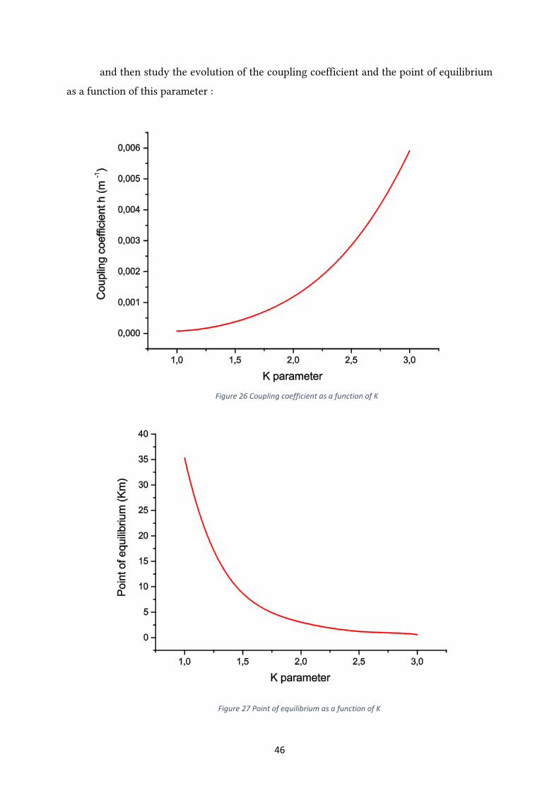
3.5.2 Refractive index perturbation :

We can write the index perturbation as a function of a parameter K as follows :

δn2(x, y) = K * 10^-2 sin(rc x)cos(rc y)

Figure 25 Crosstalk between the two propagating modes

46

and then study the evolution of the coupling coefficient and the point of equilibrium

as a function of this parameter :

Figure 26 Coupling coefficient as a function of K

Figure 27 Point of equilibrium as a function of K

47

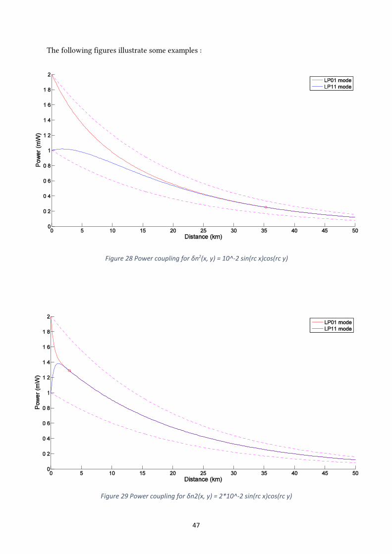
The following figures illustrate some examples :

Figure 28 Power coupling for δn2(x, y) = 10^-2 sin(rc x)cos(rc y)

Figure 29 Power coupling for δn2(x, y) = 2*10^-2 sin(rc x)cos(rc y)

48

We notice that the more significant the index perturbation, the stronger the coupling

between modes. As we increase the amplitude of the perturbation, the coupling coefficient

increases rapidly and thus the point of equilibrium decreases naturally. The previous figures

demonstrate clearly that the amplitude of the perturbation in the refractive index of the fiber

core is the most influential parameter in mode coupling.

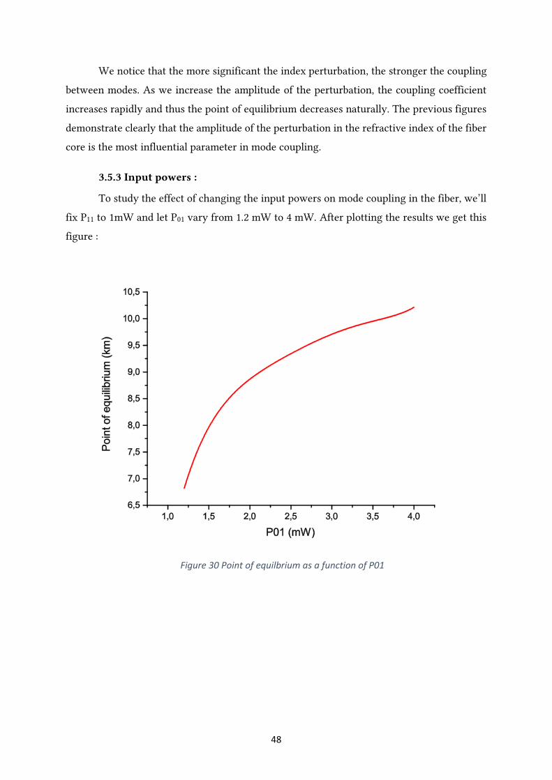
3.5.3 Input powers :

To study the effect of changing the input powers on mode coupling in the fiber, we’ll

fix P11 to 1mW and let P01 vary from 1.2 mW to 4 mW. After plotting the results we get this

figure :

Figure 30 Point of equilbrium as a function of P01

49

The following figures illustrate some examples :

Input powers do not affect the coupling coefficients, but increasing the difference

between lunch powers can help by increasing the value of the point of equilibrium. Such

Figure 31 Power coupling for P01=4mW and P11=1mW

Figure 32 Power coupling for P01=1.2mW and P11=1mW

50

solution should be a last resort since increasing the system’s reach using this method will

increase the energy cost and there is always the limit imposed by the nonlinear effects that

rise as we increase the power injected in the fiber.

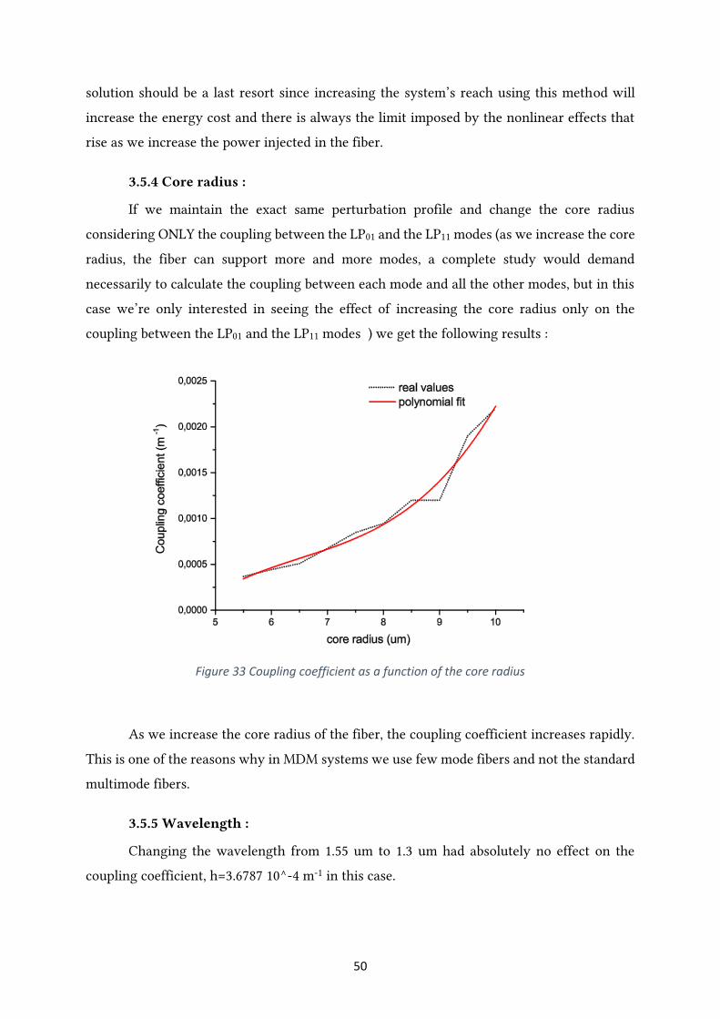
3.5.4 Core radius :

If we maintain the exact same perturbation profile and change the core radius

considering ONLY the coupling between the LP01 and the LP11 modes (as we increase the core

radius, the fiber can support more and more modes, a complete study would demand

necessarily to calculate the coupling between each mode and all the other modes, but in this

case we’re only interested in seeing the effect of increasing the core radius only on the

coupling between the LP01 and the LP11 modes ) we get the following results :

As we increase the core radius of the fiber, the coupling coefficient increases rapidly.

This is one of the reasons why in MDM systems we use few mode fibers and not the standard

multimode fibers.

3.5.5 Wavelength :

Changing the wavelength from 1.55 um to 1.3 um had absolutely no effect on the

coupling coefficient, h=3.6787 10^-4 m-1 in this case.

Figure 33 Coupling coefficient as a function of the core radius

51

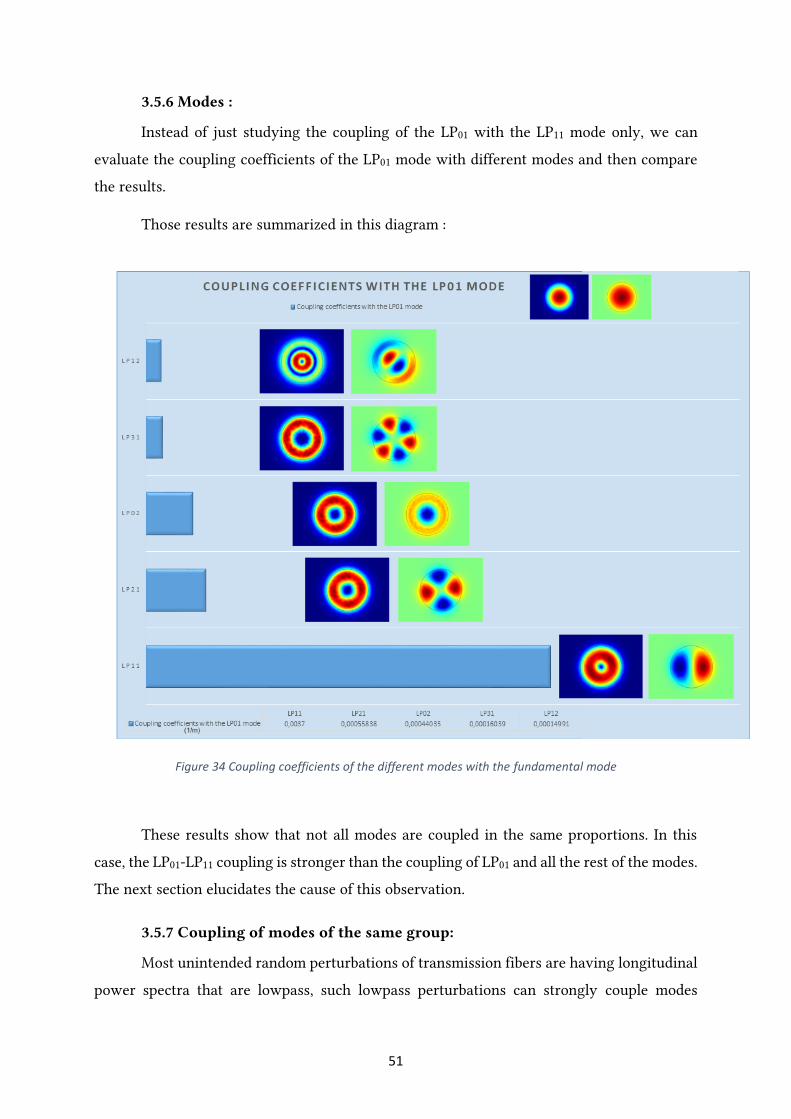
3.5.6 Modes :

Instead of just studying the coupling of the LP01 with the LP11 mode only, we can

evaluate the coupling coefficients of the LP01 mode with different modes and then compare

the results.

Those results are summarized in this diagram :

Figure 34 Coupling coefficients of the different modes with the fundamental mode

These results show that not all modes are coupled in the same proportions. In this

case, the LP01-LP11 coupling is stronger than the coupling of LP01 and all the rest of the modes.

The next section elucidates the cause of this observation.

3.5.7 Coupling of modes of the same group:

Most unintended random perturbations of transmission fibers are having longitudinal

power spectra that are lowpass, such lowpass perturbations can strongly couple modes

52

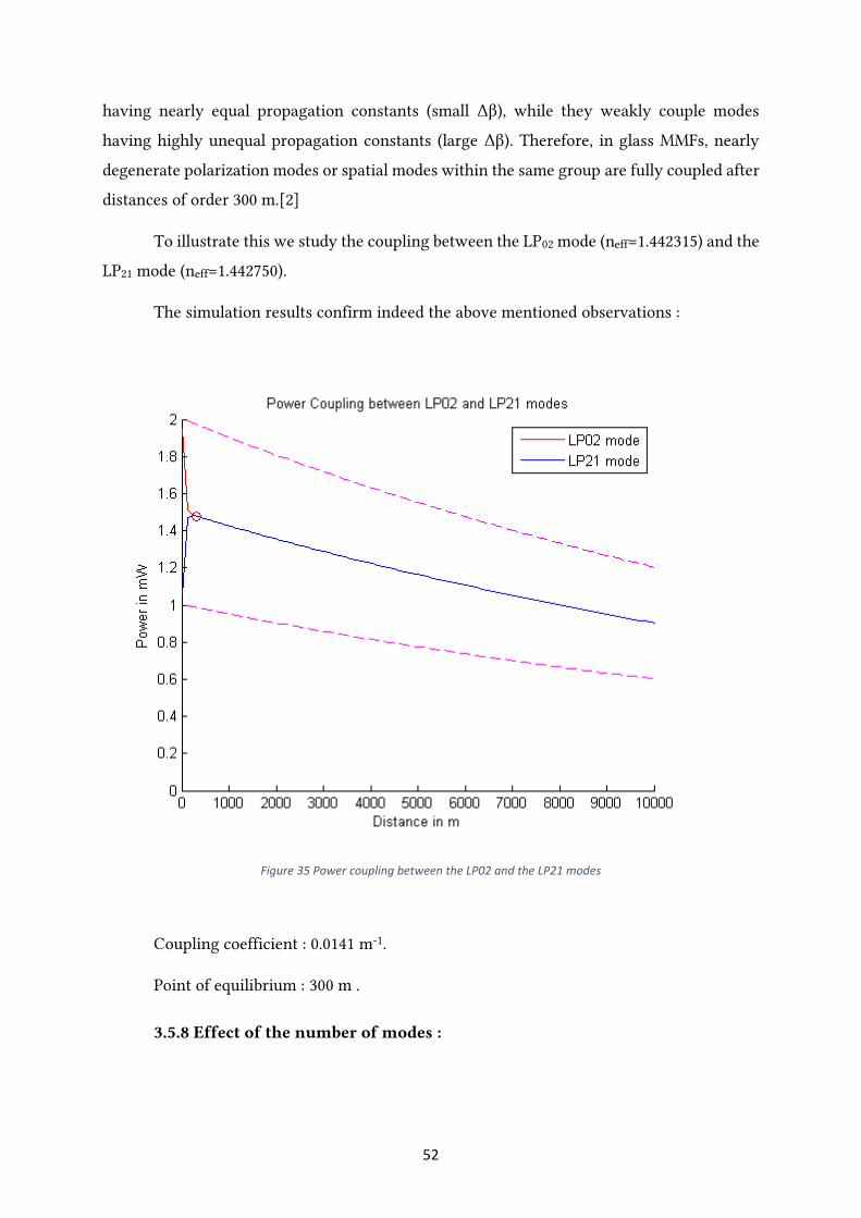
having nearly equal propagation constants (small Δβ), while they weakly couple modes

having highly unequal propagation constants (large Δβ). Therefore, in glass MMFs, nearly

degenerate polarization modes or spatial modes within the same group are fully coupled after

distances of order 300 m.[2]

To illustrate this we study the coupling between the LP02 mode (neff=1.442315) and the

LP21 mode (neff=1.442750).

The simulation results confirm indeed the above mentioned observations :

Figure 35 Power coupling between the LP02 and the LP21 modes

Coupling coefficient : 0.0141 m-1.

Point of equilibrium : 300 m .

3.5.8 Effect of the number of modes :

53

In this section we’ll be treating more than two modes, therefore more than two

coupled differential equations, it is more convenient to write the system of the coupled

differential equations using a matrix notation :

(

𝑑𝑃1𝑑𝑧𝑑𝑃2𝑑𝑧⋮𝑑𝑃𝑛𝑑𝑧 )

= 𝐴𝑛 (

𝑃1𝑃2⋮𝑃𝑛

)

Where 𝐴𝑛 = (−(𝛼 + ∑ ℎ1𝑖

𝑛𝑖=2 ) ⋯ ℎ1𝑛⋮ ⋱ ⋮ℎ𝑛1 ⋯ −(𝛼 + ∑ ℎ𝑛𝑖

𝑛−1𝑖=1 )

)

The general solution of such a system is :

𝑃 = 𝐶1𝑉1𝑒𝜆1𝑧 + 𝐶2𝑉2𝑒

𝜆2𝑧 +⋯+ 𝐶𝑛𝑉𝑛𝑒𝜆𝑛𝑧

where:

λ1, ...,λn are the eigenvalues of the matrix An and V1,...,Vn are it’s eigenvectors.

C1 C2,...,Cn are constants and can be determined using the initial conditions of the

injected powers at the input of the fiber.

1) Four mode fiber :

For this simulation we used a fiber with a 7.5 um core radius which supports four

modes : LP01, LP11, LP21 and LP02.

54

LP01 LP11 LP21 LP02

Effective index 1.444256 1.442102 1.439425 1.438756

Table 3.1: Modes effective indices

We calculated the coupling coefficients between all modes :

Coupl.coeff (m-1) LP01 LP11 LP21 LP02

LP01 — 8.3249e-04 1.2690e-04 9.2291e-05

LP11 8.3249e-04 — 5.7740e-04 2.3651e-04

LP21 1.2690e-04 5.7740e-04 — 0.0065

LP02 9.2291e-05 2.3651e-04 0.0065 —

Table 3.2: Coupling coefficients for the different modes

We then implemented and solved the above mentioned system of coupled differential

equations. The obtained solutions are illustrated in the following figure :

Figure 36 Power coupling in a four mode fiber

55

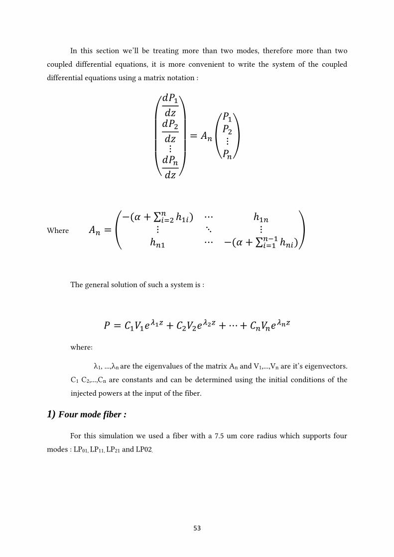
2) Six mode fiber :

Following the exact same steps as in the case of the four mode fiber, we made another

simulation, this time with a fiber that has a 12 um core radius supporting six modes.

This time we also tried different lunch power combinations to highlight even more

the coupling between the different modes, especially how it is stronger between modes having

close propagation constants.

The results are illustrated in the following figures :

Figure 37 Power coupling in a six mode fiber (first configuration)

56

Figure 38 Power coupling in a six mode fiber (second configuration)

Figure 39 Power coupling in a six mode fiber (third configuration)

57

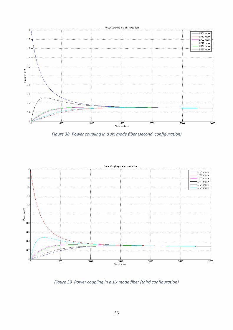
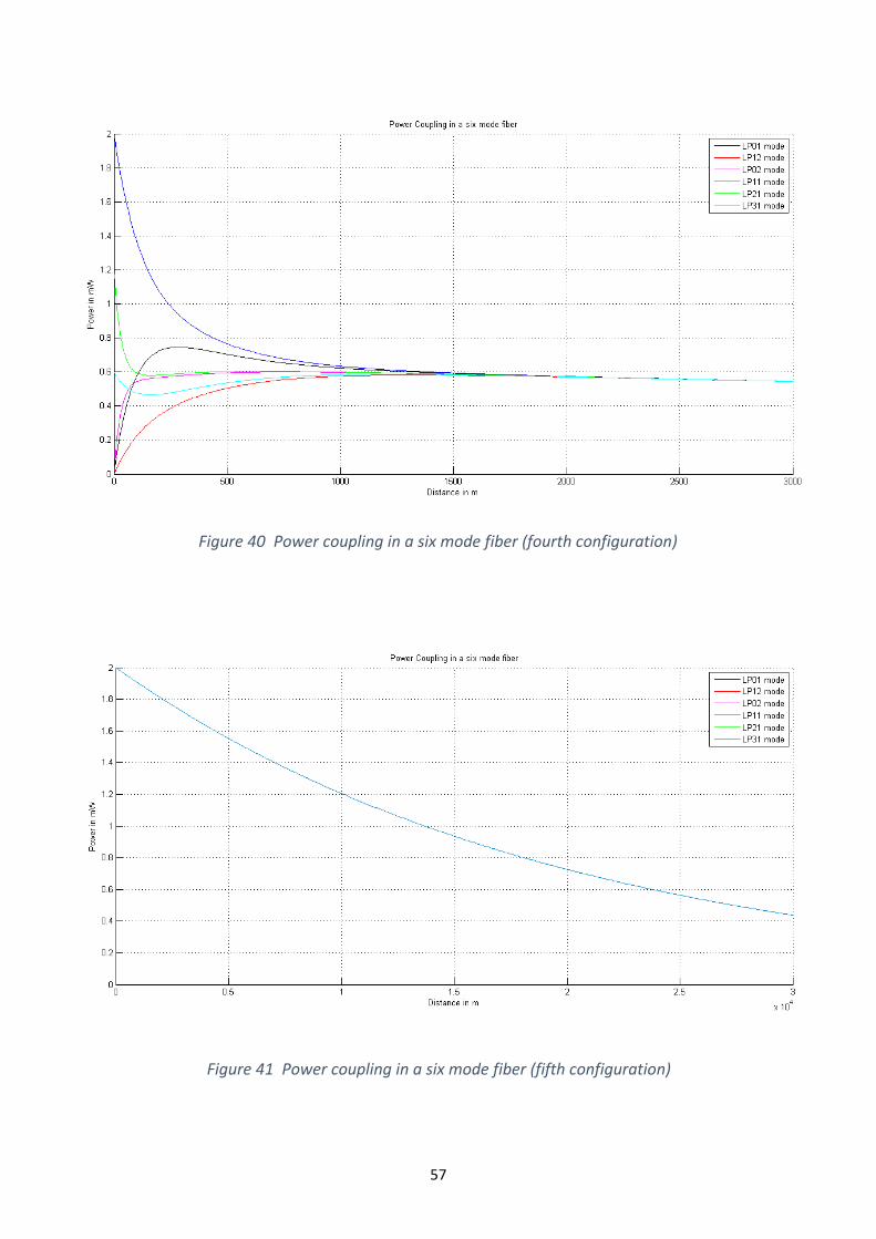
Figure 40 Power coupling in a six mode fiber (fourth configuration)

Figure 41 Power coupling in a six mode fiber (fifth configuration)

58

The previous figures illustrate that in MDM systems, the more modes we use, the

more transmission channels we have. Unfortunately, as illustrated by the previous figures,

this has an obvious disadvantage : in a two mode fiber, each mode is only coupled with one

other mode while in six mode fiber each mode is coupled with five other modes. Not to

mention the increase in the coupling coefficients when we increase the core radius.

These figures also illustrate more how modes of the same group tend to couple

stronger than the other modes. One exception is the last figure. This figure illustrates how

mode coupling tends to make an equilibrium between mode powers. If this equilibrium is

established from the beginning (if we lunch all modes with the same initial power) there will

always be mode coupling, but it will preserve this power equilibrium throughout the rest of

the distance of propagation.

3.6 Conclusion :

In this chapter we studied the performance of an MDM system by evaluating the main

obstacle for MDM transmission which is ‘mode coupling’, as a function of the different

possible parameters. We then interpreted the obtained numerical results in order to determine

how to optimize a transmission system over FMF for the best MDM efficiency.

Conclusion : In this report we studied the concept of optical mode division multiplexed

transmission systems. The continuously increasing demand for worldwide data traffic

requires new, disruptive technologies in optical transmission systems, and mode division

multiplexing (MDM) is one of the candidates currently drawing a lot of attention from

researchers all over the world.

MDM is a special form of space division multiplexing (SDM) and it has been shown

that compared to other SDM techniques, MDM offers a relatively high potential for synergies,

but at the same time, it also comes along with the highest amount of uncertainty of all SDM

solutions concerning its feasibility. It requires fundamental changes in system design (FMF,

mode multiplexer and demultiplexer, MIMO digital signal processing) and comes along with

new transmission limiting effects compared to systems relying on single mode fiber (SMF).

Today the biggest challenge is linear mode coupling leading to intermodal crosstalk in

59

combination with a high differential mode group delay (DMGD) between different spatial

modes.

In this project we focused primarily on a weakly coupled MDM approach where we

try to minimize mode coupling as much as possible and rely on the maximum required MIMO

DSP to compensate for the high DMGD. This is why our main focus was on optimizing system

parameters to minimize mode coupling as much as possible in order to be able to physically

separate the signals of the different spatial modes at the receiving end.

Unfortunately we had no experimental setup to actually perform any MDM

transmission experiments, so we used the coupled power theory to model mathematically the

coupling phenomena that occurs during the propagation of the different modes in the fiber.

We then used a finite element analysis solver to simulate a FMF and obtained the numerical

results presented in this report.

Finally, after analyzing and interpreting these results we proposed the optimal

configuration for each studied system parameter that result in the lowest levels of mode

coupling.

60

4. Bibliography :

[1] http://www.rp-photonics.com/

[2] J. M. Kahn, Keang-Po Ho and M. Bagher Shemirani"Mode Coupling Effects in Multi-Mode

Fibers" Proc. of Optical Fiber Commun. Conf., Los Angeles, CA, March 4-8, 2013

[3] Fedor Mitschke, ‘Fiber optics : physics and technology’, Springer, 2009

[4] A.Yariv and P.Yeh Optical Electronics in Modern Communications, sixth Edition

(Academic Press, 2007).

[5] D. Marcuse, ‘Theory of Dielectric Optical Waveguide’ second ed, Academic press,1997

[6] D. J. Richardson, J. M. Fini and L E. Nelson, ‘Space Division Multiplexing in Optical Fibres’

[7] P. J. Winzer, ‘Optical Networking Beyond WDM’, IEEE Photonics J. 4, 647 (2012)

[8] John Crisp and Barry Elliot, ‘Introduction to fiber optics’ , 3rd edition, Elsevier

[9] Christos P. Tsekrekos, Mode group diversity multiplexing in multimode fiber transmission

systems, thesis

[10] " Cisco Visual Networking Index-Forecast and Methodology, 2007-2012," Cisco Systems,

Inc., May 2013.