2D Transient Conduction CalculatorUsing MatlabGreg TeichertKyle Halgren

Assumptions Use Finite Difference Equations shown in

table 5.2 2D transient conduction with heat

transfer in all directions (i.e. no internal corners as shown in the second condition in table 5.2)

Uniform temperature gradient in object Only rectangular geometry will be

analyzed

Program Inputs The calculator asks for

Length of sides (a, b) (m) Outside Temperatures (T_inf 1-T_inf 4) (K) Temperature of object (T_0) (K) Thermal Convection Coefficient (h1-h4)

(W/m^2*K) Thermal Conduction Coefficient (k) (W/m*K) Density (ρ) (kg/m^3) Specific Heat (Cp) (J/kg*K) Desired Time Interval (t) (s)

Transient Conduction Example problem

suppose we have an object with rectangular cross-section with these boundary conditions:

T_inf 1, h1

T_inf 2, h2

T_inf 3, h3

T_inf 4, h4

a

b

Origin

Conditions%Userdefined h valuesh(1) = 10;h(2) = .1;h(3) = 10;h(4) = .1; %Boundary conditions%Userdefined T infinity values in kelvinT_inf(1) = 293;T_inf(2) = 293;T_inf(3) = 353;T_inf(4) = 353; %Initial condition (assume uniform initial temperature)%Userdefined initial temperature valueT_0 = 573; %Material properties%Userdefined material valuesk = .08;rho = 7480;c_p = .460; %Userdefined physical variablesa = 1; %height of cross sectionb = 1.3; %width of cross sectiont = 3600; %time at which results are given

Time Step (Δt) We assumed a value of Δx = Δy =

gcd(a, b) Using each of the conditions (except the

second) in the table 5.2, we calculate the Δt and choose the smallest value

Using that Δt we calculate Fo Our outputs for delta_x, delta_t, Fo

respectively 0.0500, 3.7078, 0.0345

Method Using the Finite Difference Method,

matlab generates a matrix of temperature values that are represented in the graph shown on the next slide

This method allows for the calculation of every node in any 2D direction

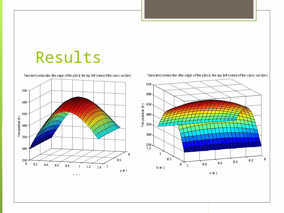
Results

0

0.5

10 0.2 0.4 0.6 0.8 1 1.2 1.4

250

300

350

400

450

500

550

a (m)

b (m)

Transient conduction (the origin of the plot is the top left corner of the cross section)

Tem

pera

ture

(K)

00.20.40.60.810

0.5

1

1.5250

300

350

400

450

500

550

a (m)

Transient conduction (the origin of the plot is the top left corner of the cross section)

b (m)

Tem

pera

ture

(K

)

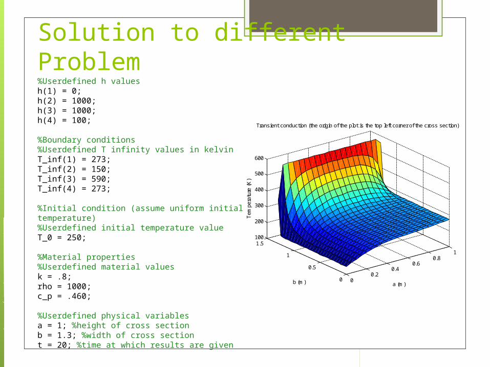
Solution to different Problem%Userdefined h valuesh(1) = 0;h(2) = 1000;h(3) = 1000;h(4) = 100; %Boundary conditions%Userdefined T infinity values in kelvinT_inf(1) = 273;T_inf(2) = 150;T_inf(3) = 590;T_inf(4) = 273; %Initial condition (assume uniform initial temperature)%Userdefined initial temperature valueT_0 = 250; %Material properties%Userdefined material valuesk = .8;rho = 1000;c_p = .460; %Userdefined physical variablesa = 1; %height of cross sectionb = 1.3; %width of cross sectiont = 20; %time at which results are given

00.2

0.40.6

0.81

0

0.5

1

1.5100

200

300

400

500

600

a (m)

Transient conduction (the origin of the plot is the top left corner of the cross section)

b (m)

Tem

pera

ture

(K

)

Conclusion and Recommendations Works only in rectangular geometry High values of h and t>1 causes errors

to occur due to lack of memory Use a better method to find Δx and Δt

Appendix-References Incropera, Frank P. DeWitt, DaviD P.

Fundamentals of Heat and Mass Transfer Fifth Edition, R. R. Donnelley & Sons Company. 2002 John Wiley & Sons, Inc

Appendix-hand work

Appendix-hand work