2D & 3D particle size analysis of micro-CT images

G. van Dalen, M.W. Koster

Unilever Research & Development, Advanced Measurement & Data Modelling, Olivier van Noortlaan 120, NL-3133AT Vlaardingen, Gerard-van.Dalen@unilever.com

Introduction Particles are everywhere in our everyday life. Particles can be found in nearly all products. For example bubbles in aerated products 1, water or oil droplets in emulsions, grains in cereals, salt crystals in bouillon cubes and granules in washing powders. Particles may be dispersed in a continuous phase, which in consumer products is mostly air or water. The size of these particles may influence the physical, chemical or physiological behaviour of products or processes. A wide variety of different techniques are used to measure the particle size distribution. These include physical, electrical, imaging and optical techniques. Imaging techniques with image analysis offer the possibility to analyse the size and shape of each individual particle present in a sample. Especially X-ray microtomography (μCT) provides a powerful tool for non-destructive analysis in 3D. Various image analysis methods are used to obtain quantitative information about the size and shape of particles. In this paper 2D and 3D discrete image analysis methods are compared. For each particle a variety of different specific measurements can be made (e.g. location, size and shape)2. In these methods touching particles are separated, so that each individual particle can be identified, counted and measured. In the SkyScan CT-Analyser (CTan) software the separation possibilities are limited. Therefore, it was investigated if the determination of the 3D structure thickness can be used as an indirect method for the estimation of the particle size distribution. These methods were tested on μCT images of aerated emulsions imaged at different storage times3. The bubble size of these samples increases in time (coarsening). This will not only change the mean bubble size, but also the shape of the size distribution curve.

Methods Images were obtained using a SkyScan 1172 desktop µCT system. Details about the imaging acquisition and tomographic reconstruction can be found in a separate paper3. The image analysis methods were tested on identical binary images to exclude influences of different thresholding procedures. For 2D and 3D image analysis of the individual particles, the image analysis toolbox DIPlib (vers. 2.3) from the Delft University of Technology, running under MATlab (vers. 2009a) from MathWorks was used. Also Avizo Fire (vers. 7.0) from the Visualization Sciences Group was used for 3D image analysis of the indivual particles. Avizo Fire combines 3D visualisation with 3D quantitative measurement. For visualisation in 3D space, isosurface rendering was used. Images of time series were aligned in Avizo Fire using affine registration. Before registration a coarse manual alignment was performed using marks on the sample holder wall. The 3D structure thickness was analysed using SkyScan CT-Analyser (CTan) version 1.11.10.0.

2D image analysis A 2D image will not represent the true sizes of objects. Also the number of objects observed in a 2D image does not correspond to the number per unit volume. A 2D image is the intersection of a plane with the three-dimensional space. The observed apparent size distribution is generally different from the true distribution because: - The apparent diameters are as a rule equal or smaller than the true diameters (with a

random section the plane may pass through the sphere at the equator, near one of the poles, or anywhere in between)

- A random section will contain a relatively greater number of actually large droplets than of small ones (compared to the true distribution), because the former will more frequently be intersected by the section plane.

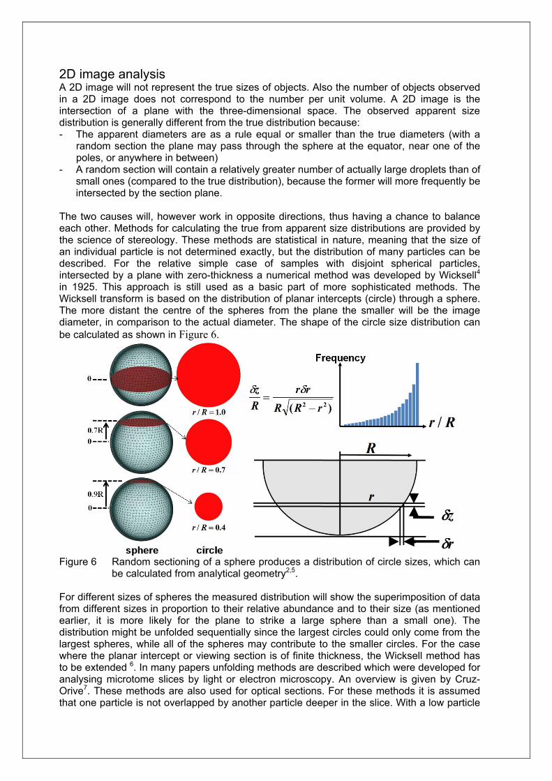
The two causes will, however work in opposite directions, thus having a chance to balance each other. Methods for calculating the true from apparent size distributions are provided by the science of stereology. These methods are statistical in nature, meaning that the size of an individual particle is not determined exactly, but the distribution of many particles can be described. For the relative simple case of samples with disjoint spherical particles, intersected by a plane with zero-thickness a numerical method was developed by Wicksell4 in 1925. This approach is still used as a basic part of more sophisticated methods. The Wicksell transform is based on the distribution of planar intercepts (circle) through a sphere. The more distant the centre of the spheres from the plane the smaller will be the image diameter, in comparison to the actual diameter. The shape of the circle size distribution can be calculated as shown in Figure 6.

Figure 6 Random sectioning of a sphere produces a distribution of circle sizes, which can

be calculated from analytical geometry2,5. For different sizes of spheres the measured distribution will show the superimposition of data from different sizes in proportion to their relative abundance and to their size (as mentioned earlier, it is more likely for the plane to strike a large sphere than a small one). The distribution might be unfolded sequentially since the largest circles could only come from the largest spheres, while all of the spheres may contribute to the smaller circles. For the case where the planar intercept or viewing section is of finite thickness, the Wicksell method has to be extended 6. In many papers unfolding methods are described which were developed for analysing microtome slices by light or electron microscopy. An overview is given by Cruz-Orive7. These methods are also used for optical sections. For these methods it is assumed that one particle is not overlapped by another particle deeper in the slice. With a low particle

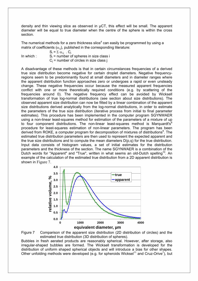
density and thin viewing slice as observed in μCT, this effect will be small. The apparent diameter will be equal to true diameter when the centre of the sphere is within the cross section. The numerical methods for a zero thickness slice4 can easily be programmed by using a matrix of coefficients (i,j), published in the corresponding literature: Si = i,j . Cj In which : Si = number of spheres in size class i Cj = number of circles in size class j A disadvantage of these methods is that in certain circumstances frequencies of a derived true size distribution become negative for certain droplet diameters. Negative frequency-regions seem to be predominantly found at small diameters and in diameter ranges where the apparent distribution function approaches zero or undergoes a rapid or even unsteady change. These negative frequencies occur because the measured apparent frequencies conflict with one or more theoretically required conditions (e.g. by scattering of the frequencies around 0). The negative frequency effect can be avoided by Wicksell transformation of true log-normal distributions (see section about size distributions). The observed apparent size distribution can now be fitted by a linear combination of the apparent size distributions derived analytically from the log-normal distributions, in order to estimate the parameters of the true size distribution (iterative process from initial to final parameter estimates). This procedure has been implemented in the computer program SGYNWAER using a non-linear least-squares method for estimation of the parameters of a mixture of up to four component distributions. The non-linear least-squares method is Marquardt's8 procedure for least-squares estimation of non-linear parameters. The program has been derived from ROKE, a computer program for decomposition of mixtures of distributions9. The estimated true distribution parameters are then used to represent the expected apparent and the true size distributions and to compute the mean diameters D(p,q) for the true distribution. Input data consists of histogram values, a set of initial estimates for the distribution parameters and the thickness of the section. The name SGYNWAER is a combination of the Dutch words for "Apparent" and "True", written in what seems an old-Dutch spelling10. An example of the calculation of the estimated true distribution from a 2D apparent distribution is shown in Figure 7.

Figure 7 Comparison of the apparent size distribution (2D distribution of circles) and the

estimated true distribution (3D distribution of spheres). Bubbles in fresh aerated products are reasonably spherical. However, after storage, also irregular-shaped bubbles are formed. The Wicksell transformation is developed for the distribution of uniform shaped spherical objects and will introduce a bias for other shapes. Other unfolding methods were developed (e.g. for spheroids Wicksel11 and Cruz-Orive7), but

0.0

0.5

1.0

1.5

2.0

2.5

3.0

3.5

4.0

0 1000 2000 3000 4000

rela

tiv

e v

olu

me

, %

equivalent diameter, µm

trueapparent

these models are only useful when the three-dimensional shape of the objects is known and is the same for all objects present. Unless the inherent 3D nature of the microstructure is recognised and carefully accounted for the use of 2D image analysis methods can lead to significant errors (bias).

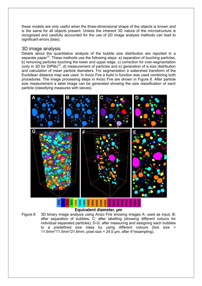
3D image analysis Details about the quantitative analysis of the bubble size distribution are reported in a separate paper12. These methods use the following steps: a) separation of touching particles, b) removing particles touching the lower and upper edge, c) correction for over-segmentation (only in 3D for DIPlib)12, d) measurement of particles and e) generation of a size distribution and calculation of mean particle diameters. For segmentation a watershed transform of the Euclidean distance map was used. In Avizo Fire a build in function was used combining both procedures. The image processing steps in Avizo Fire are shown in Figure 8. After particle size measurement a label image can be generated showing the size classification of each particle (classifying measures with sieves).

Figure 8 3D binary image analysis using Avizo Fire showing images A: used as input, B:

after separation of bubbles, C: after labelling (showing different colours for individual separated particles), D-G: after measuring and assigning each bubbles to a predefined size class by using different colours (box size = 11.5mm*11.5mm*21.6mm, pixel size = 24.0 μm, after 4*resampling).

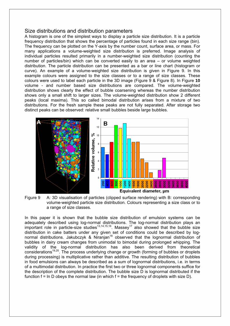
Size distributions and distribution parameters A histogram is one of the simplest ways to display a particle size distribution. It is a particle frequency distribution that shows the percentage of particles found in each size range (bin). The frequency can be plotted on the Y-axis by the number count, surface area, or mass. For many applications a volume-weighted size distribution is preferred. Image analysis of individual particles resulted primarily in a number-weighted size distribution (counting the number of particles/bin) which can be converted easily to an area – or volume weighted distribution. The particle distribution can be presented as a bar or line chart (histogram or curve). An example of a volume-weighted size distribution is given in Figure 9. In this example colours were assigned to the size classes or to a range of size classes. These colours were used to label each particle in the 3D image (Figure 9 & Figure 8). In Figure 10 volume - and number based size distributions are compared. The volume-weighted distribution shows clearly the effect of bubble coarsening whereas the number distribution shows only a small shift to larger sizes. The volume-weighted distribution show 2 different peaks (local maxima). This so called bimodal distribution arises from a mixture of two distributions. For the fresh sample these peaks are not fully separated. After storage two distinct peaks can be observed: relative small bubbles beside large bubbles.

Figure 9 A: 3D visualisation of particles (clipped surface rendering) with B: corresponding

volume-weighted particle size distribution. Colours representing a size class or to a range of size classes.

In this paper it is shown that the bubble size distribution of emulsion systems can be adequately described using log-normal distributions. The log-normal distribution plays an important role in particle-size studies13,14,15,16. Massey17 also showed that the bubble size distribution in cake batters under any given set of conditions could be described by log-normal distributions. Jakubczyk & Niranjan18 observed that the lognormal distribution of bubbles in dairy cream changes from unimodal to bimodal during prolonged whipping. The validity of the log-normal distribution has also been derived from theoretical considerations19,20. The process underlying change or growth (forming of bubbles or droplets during processing) is multiplicative rather than additive. The resulting distribution of bubbles in food emulsions can always be described as a sum of lognormal distributions, i.e. in terms of a multimodal distribution. In practice the first two or three lognormal components suffice for the description of the complete distribution. The bubble size D is lognormal distributed if the function f = ln D obeys the normal law (in which f = the frequency of droplets with size D).

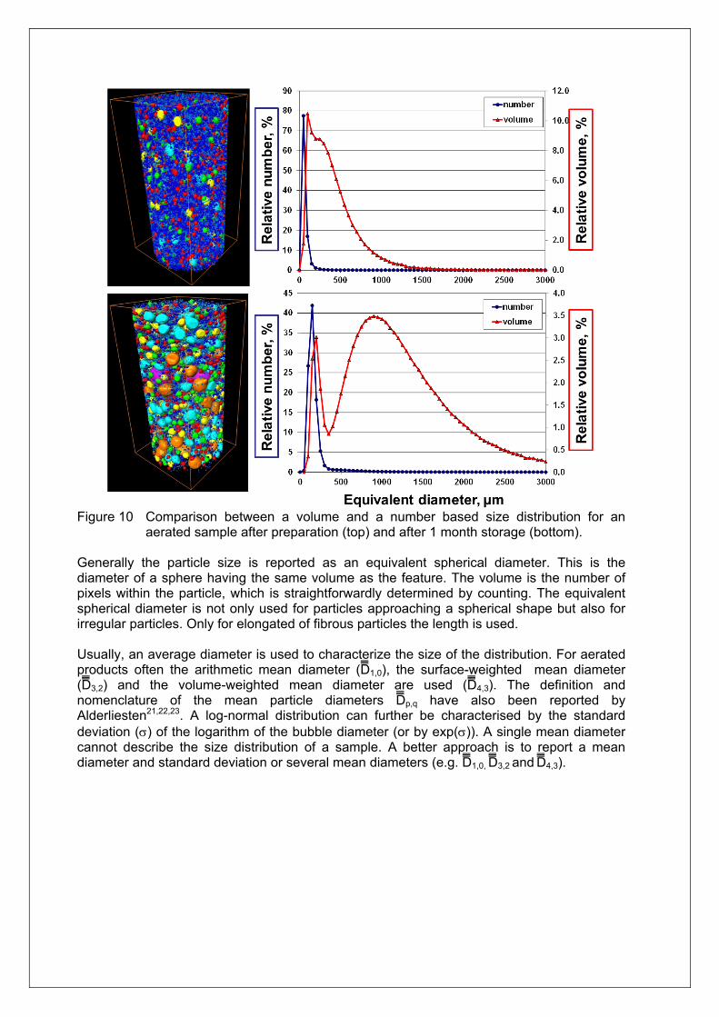
Figure 10 Comparison between a volume and a number based size distribution for an

aerated sample after preparation (top) and after 1 month storage (bottom). Generally the particle size is reported as an equivalent spherical diameter. This is the diameter of a sphere having the same volume as the feature. The volume is the number of pixels within the particle, which is straightforwardly determined by counting. The equivalent spherical diameter is not only used for particles approaching a spherical shape but also for irregular particles. Only for elongated of fibrous particles the length is used. Usually, an average diameter is used to characterize the size of the distribution. For aerated products often the arithmetic mean diameter (D̅̅̅1,0), the surface-weighted mean diameter (D̅̅̅3,2) and the volume-weighted mean diameter are used (D̅̅̅4,3). The definition and nomenclature of the mean particle diameters D̅̅̅p,q have also been reported by Alderliesten21,22,23. A log-normal distribution can further be characterised by the standard deviation () of the logarithm of the bubble diameter (or by exp()). A single mean diameter cannot describe the size distribution of a sample. A better approach is to report a mean diameter and standard deviation or several mean diameters (e.g. D̅̅̅1,0, D̅̅̅3,2 and D̅̅̅4,3).

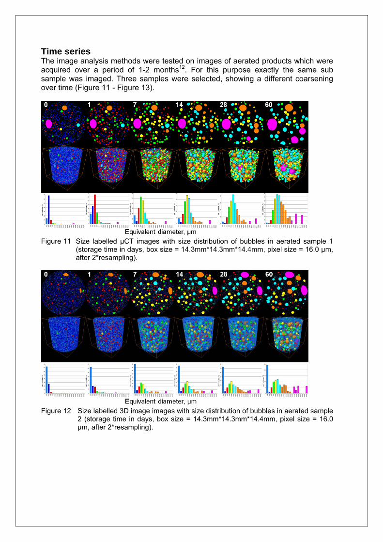
Time series The image analysis methods were tested on images of aerated products which were acquired over a period of 1-2 months12. For this purpose exactly the same sub sample was imaged. Three samples were selected, showing a different coarsening over time (Figure 11 - Figure 13).

Figure 11 Size labelled μCT images with size distribution of bubbles in aerated sample 1

(storage time in days, box size = 14.3mm*14.3mm*14.4mm, pixel size = 16.0 μm, after 2*resampling).

Figure 12 Size labelled 3D image images with size distribution of bubbles in aerated sample

2 (storage time in days, box size = 14.3mm*14.3mm*14.4mm, pixel size = 16.0 μm, after 2*resampling).

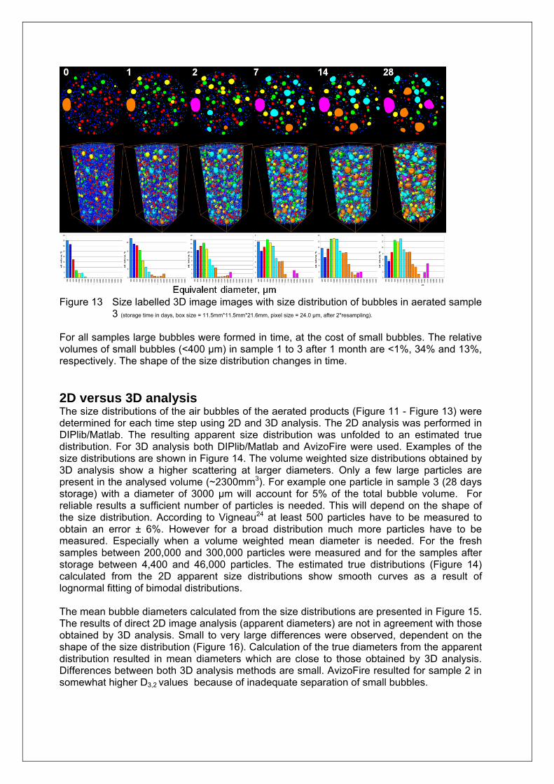
Figure 13 Size labelled 3D image images with size distribution of bubbles in aerated sample

3 (storage time in days, box size = 11.5mm*11.5mm*21.6mm, pixel size = 24.0 μm, after 2*resampling). For all samples large bubbles were formed in time, at the cost of small bubbles. The relative volumes of small bubbles (<400 µm) in sample 1 to 3 after 1 month are <1%, 34% and 13%, respectively. The shape of the size distribution changes in time.

2D versus 3D analysis The size distributions of the air bubbles of the aerated products (Figure 11 - Figure 13) were determined for each time step using 2D and 3D analysis. The 2D analysis was performed in DIPlib/Matlab. The resulting apparent size distribution was unfolded to an estimated true distribution. For 3D analysis both DIPlib/Matlab and AvizoFire were used. Examples of the size distributions are shown in Figure 14. The volume weighted size distributions obtained by 3D analysis show a higher scattering at larger diameters. Only a few large particles are present in the analysed volume (~2300mm3). For example one particle in sample 3 (28 days storage) with a diameter of 3000 µm will account for 5% of the total bubble volume. For reliable results a sufficient number of particles is needed. This will depend on the shape of the size distribution. According to Vigneau24 at least 500 particles have to be measured to obtain an error ± 6%. However for a broad distribution much more particles have to be measured. Especially when a volume weighted mean diameter is needed. For the fresh samples between 200,000 and 300,000 particles were measured and for the samples after storage between 4,400 and 46,000 particles. The estimated true distributions (Figure 14) calculated from the 2D apparent size distributions show smooth curves as a result of lognormal fitting of bimodal distributions. The mean bubble diameters calculated from the size distributions are presented in Figure 15. The results of direct 2D image analysis (apparent diameters) are not in agreement with those obtained by 3D analysis. Small to very large differences were observed, dependent on the shape of the size distribution (Figure 16). Calculation of the true diameters from the apparent distribution resulted in mean diameters which are close to those obtained by 3D analysis. Differences between both 3D analysis methods are small. AvizoFire resulted for sample 2 in somewhat higher D3,2 values because of inadequate separation of small bubbles.

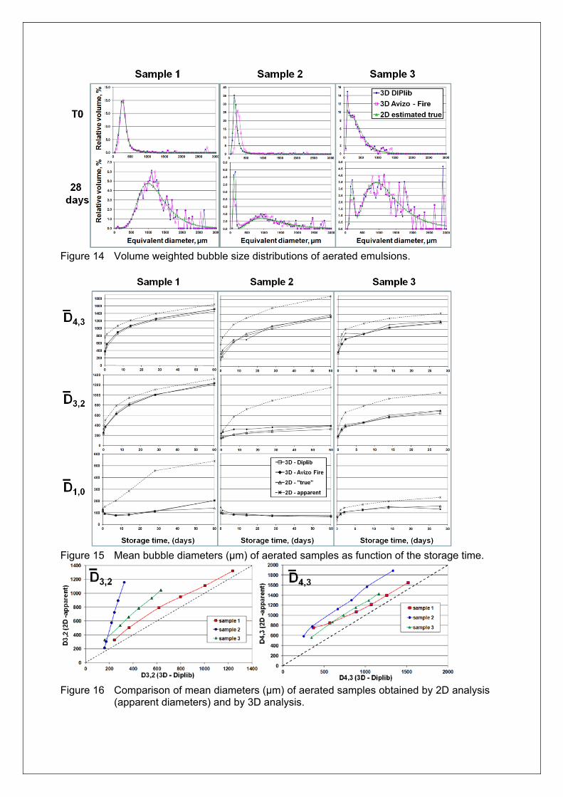
Figure 14 Volume weighted bubble size distributions of aerated emulsions.

Figure 15 Mean bubble diameters (µm) of aerated samples as function of the storage time.

Figure 16 Comparison of mean diameters (µm) of aerated samples obtained by 2D analysis

(apparent diameters) and by 3D analysis.

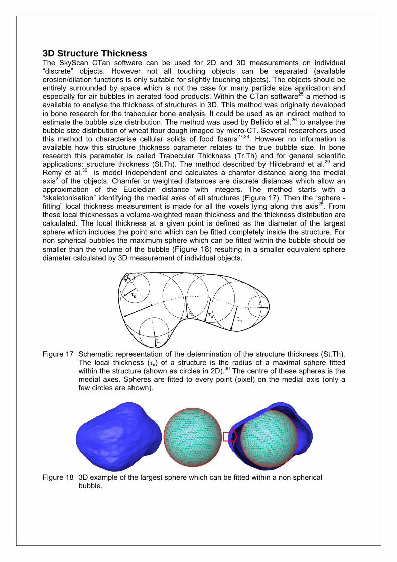
3D Structure Thickness The SkyScan CTan software can be used for 2D and 3D measurements on individual “discrete” objects. However not all touching objects can be separated (available erosion/dilation functions is only suitable for slightly touching objects). The objects should be entirely surrounded by space which is not the case for many particle size application and especially for air bubbles in aerated food products. Within the CTan software25 a method is available to analyse the thickness of structures in 3D. This method was originally developed in bone research for the trabecular bone analysis. It could be used as an indirect method to estimate the bubble size distribution. The method was used by Bellido et al.26 to analyse the bubble size distribution of wheat flour dough imaged by micro-CT. Several researchers used this method to characterise cellular solids of food foams27,28. However no information is available how this structure thickness parameter relates to the true bubble size. In bone research this parameter is called Trabecular Thickness (Tr.Th) and for general scientific applications: structure thickness (St.Th). The method described by Hildebrand et al.29 and Remy et al.30 is model independent and calculates a chamfer distance along the medial axis2 of the objects. Chamfer or weighted distances are discrete distances which allow an approximation of the Eucledian distance with integers. The method starts with a “skeletonisation” identifying the medial axes of all structures (Figure 17). Then the “sphere -fitting” local thickness measurement is made for all the voxels lying along this axis25. From these local thicknesses a volume-weighted mean thickness and the thickness distribution are calculated. The local thickness at a given point is defined as the diameter of the largest sphere which includes the point and which can be fitted completely inside the structure. For non spherical bubbles the maximum sphere which can be fitted within the bubble should be smaller than the volume of the bubble (Figure 18) resulting in a smaller equivalent sphere diameter calculated by 3D measurement of individual objects.

Figure 17 Schematic representation of the determination of the structure thickness (St.Th).

The local thickness (τn) of a structure is the radius of a maximal sphere fitted within the structure (shown as circles in 2D).30 The centre of these spheres is the medial axes. Spheres are fitted to every point (pixel) on the medial axis (only a few circles are shown).

Figure 18 3D example of the largest sphere which can be fitted within a non spherical

bubble.

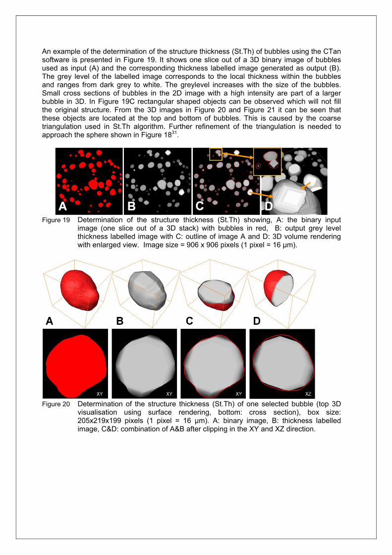
An example of the determination of the structure thickness (St.Th) of bubbles using the CTan software is presented in Figure 19. It shows one slice out of a 3D binary image of bubbles used as input (A) and the corresponding thickness labelled image generated as output (B). The grey level of the labelled image corresponds to the local thickness within the bubbles and ranges from dark grey to white. The greylevel increases with the size of the bubbles. Small cross sections of bubbles in the 2D image with a high intensity are part of a larger bubble in 3D. In Figure 19C rectangular shaped objects can be observed which will not fill the original structure. From the 3D images in Figure 20 and Figure 21 it can be seen that these objects are located at the top and bottom of bubbles. This is caused by the coarse triangulation used in St.Th algorithm. Further refinement of the triangulation is needed to approach the sphere shown in Figure 1831.

Figure 19 Determination of the structure thickness (St.Th) showing, A: the binary input

image (one slice out of a 3D stack) with bubbles in red, B: output grey level thickness labelled image with C: outline of image A and D: 3D volume rendering with enlarged view. Image size = 906 x 906 pixels (1 pixel = 16 µm).

Figure 20 Determination of the structure thickness (St.Th) of one selected bubble (top 3D

visualisation using surface rendering, bottom: cross section), box size: 205x219x199 pixels (1 pixel = 16 µm). A: binary image, B: thickness labelled image, C&D: combination of A&B after clipping in the XY and XZ direction.

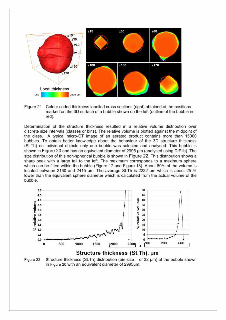
Figure 21 Colour coded thickness labelled cross sections (right) obtained at the positions

marked on the 3D surface of a bubble shown on the left (outline of the bubble in red).

Determination of the structure thickness resulted in a relative volume distribution over discrete size intervals (classes or bins). The relative volume is plotted against the midpoint of the class. A typical micro-CT image of an aerated product contains more than 15000 bubbles. To obtain better knowledge about the behaviour of the 3D structure thickness (St.Th) on individual objects only one bubble was selected and analysed. This bubble is shown in Figure 20 and has an equivalent diameter of 2995 µm (analysed using DIPlib). The size distribution of this non-spherical bubble is shown in Figure 22. This distribution shows a sharp peak with a large tail to the left. The maximum corresponds to a maximum sphere which can be fitted within the bubble (Figure 17 and Figure 18). About 80% of the volume is located between 2160 and 2415 µm. The average St.Th is 2232 µm which is about 25 % lower than the equivalent sphere diameter which is calculated from the actual volume of the bubble.

Figure 22 Structure thickness (St.Th) distribution (bin size = of 32 µm) of the bubble shown

in Figure 20 with an equivalent diameter of 2995µm.

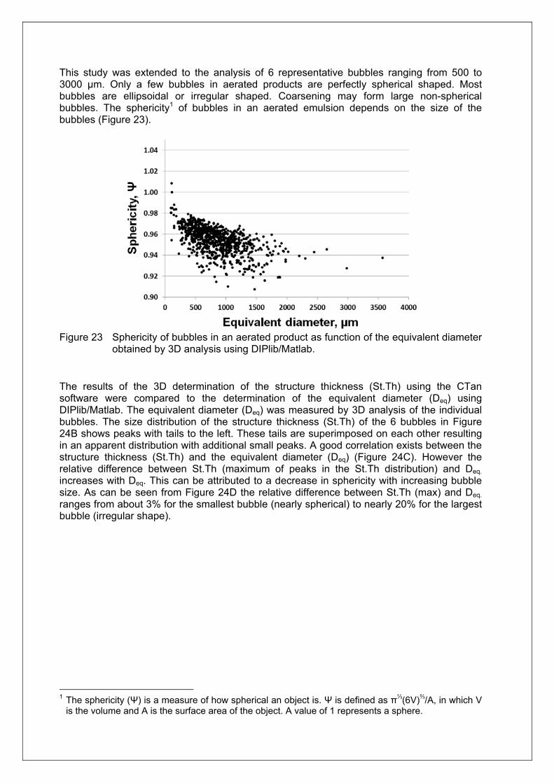
This study was extended to the analysis of 6 representative bubbles ranging from 500 to 3000 µm. Only a few bubbles in aerated products are perfectly spherical shaped. Most bubbles are ellipsoidal or irregular shaped. Coarsening may form large non-spherical bubbles. The sphericity1 of bubbles in an aerated emulsion depends on the size of the bubbles (Figure 23).

Figure 23 Sphericity of bubbles in an aerated product as function of the equivalent diameter

obtained by 3D analysis using DIPlib/Matlab. The results of the 3D determination of the structure thickness (St.Th) using the CTan software were compared to the determination of the equivalent diameter (Deq) using DIPlib/Matlab. The equivalent diameter (Deq) was measured by 3D analysis of the individual bubbles. The size distribution of the structure thickness (St.Th) of the 6 bubbles in Figure 24B shows peaks with tails to the left. These tails are superimposed on each other resulting in an apparent distribution with additional small peaks. A good correlation exists between the structure thickness (St.Th) and the equivalent diameter (Deq) (Figure 24C). However the relative difference between St.Th (maximum of peaks in the St.Th distribution) and Deq.

increases with Deq. This can be attributed to a decrease in sphericity with increasing bubble size. As can be seen from Figure 24D the relative difference between St.Th (max) and Deq. ranges from about 3% for the smallest bubble (nearly spherical) to nearly 20% for the largest bubble (irregular shape).

1 The sphericity (Ψ) is a measure of how spherical an object is. Ψ is defined as π⅓(6V)⅔/A, in which V

is the volume and A is the surface area of the object. A value of 1 represents a sphere.

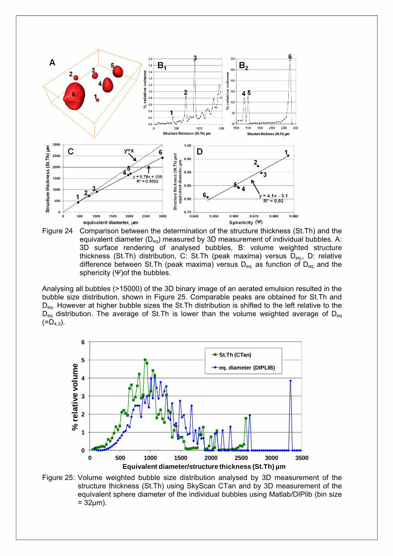
Figure 24 Comparison between the determination of the structure thickness (St.Th) and the

equivalent diameter (Deq) measured by 3D measurement of individual bubbles. A: 3D surface rendering of analysed bubbles, B: volume weighted structure thickness (St.Th) distribution, C: St.Th (peak maxima) versus Deq,, D: relative difference between St.Th (peak maxima) versus Deq, as function of Deq, and the sphericity (Ψ)of the bubbles.

Analysing all bubbles (>15000) of the 3D binary image of an aerated emulsion resulted in the bubble size distribution, shown in Figure 25. Comparable peaks are obtained for St.Th and Deq. However at higher bubble sizes the St.Th distribution is shifted to the left relative to the Deq distribution. The average of St.Th is lower than the volume weighted average of Deq (=D4,3).

Figure 25: Volume weighted bubble size distribution analysed by 3D measurement of the

structure thickness (St.Th) using SkyScan CTan and by 3D measurement of the equivalent sphere diameter of the individual bubbles using Matlab/DIPlib (bin size = 32µm).

0

1

2

3

4

5

6

0 500 1000 1500 2000 2500 3000 3500

% r

ela

tive

vo

lum

e

Equivalent diameter/structure thickness (St.Th) µm

St.Th (CTan)

eq. diameter (DIPLIB)

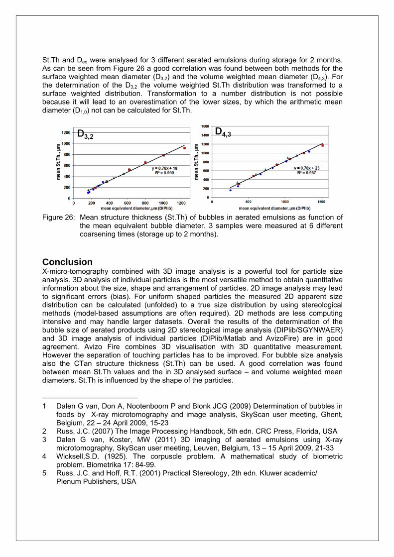
St.Th and Deq were analysed for 3 different aerated emulsions during storage for 2 months. As can be seen from Figure 26 a good correlation was found between both methods for the surface weighted mean diameter (D3,2) and the volume weighted mean diameter (D4,3). For the determination of the D3,2 the volume weighted St.Th distribution was transformed to a surface weighted distribution. Transformation to a number distribution is not possible because it will lead to an overestimation of the lower sizes, by which the arithmetic mean diameter (D1,0) not can be calculated for St.Th.

Figure 26: Mean structure thickness (St.Th) of bubbles in aerated emulsions as function of

the mean equivalent bubble diameter. 3 samples were measured at 6 different coarsening times (storage up to 2 months).

Conclusion X-micro-tomography combined with 3D image analysis is a powerful tool for particle size analysis. 3D analysis of individual particles is the most versatile method to obtain quantitative information about the size, shape and arrangement of particles. 2D image analysis may lead to significant errors (bias). For uniform shaped particles the measured 2D apparent size distribution can be calculated (unfolded) to a true size distribution by using stereological methods (model-based assumptions are often required). 2D methods are less computing intensive and may handle larger datasets. Overall the results of the determination of the bubble size of aerated products using 2D stereological image analysis (DIPlib/SGYNWAER) and 3D image analysis of individual particles (DIPlib/Matlab and AvizoFire) are in good agreement. Avizo Fire combines 3D visualisation with 3D quantitative measurement. However the separation of touching particles has to be improved. For bubble size analysis also the CTan structure thickness (St.Th) can be used. A good correlation was found between mean St.Th values and the in 3D analysed surface – and volume weighted mean diameters. St.Th is influenced by the shape of the particles. 1 Dalen G van, Don A, Nootenboom P and Blonk JCG (2009) Determination of bubbles in

foods by X-ray microtomography and image analysis, SkyScan user meeting, Ghent, Belgium, 22 – 24 April 2009, 15-23

2 Russ, J.C. (2007) The Image Processing Handbook, 5th edn. CRC Press, Florida, USA 3 Dalen G van, Koster, MW (2011) 3D imaging of aerated emulsions using X-ray

microtomography, SkyScan user meeting, Leuven, Belgium, 13 – 15 April 2009, 21-33 4 Wicksell,S.D. (1925). The corpuscle problem. A mathematical study of biometric

problem. Biometrika 17: 84-99. 5 Russ, J.C. and Hoff, R.T. (2001) Practical Stereology, 2th edn. Kluwer academic/

Plenum Publishers, USA

6 Cruz_Orive, L.M. (1983). Distribution-free estimation of sphere size distribution from

slabs showing overprojection and truncation, with a review of previous methods. J. Micros. 131: 265-290.

7 Cruz_Orive L.M. (1976). Particle size-shape distributions: the general spheroid problem, I Mathematical model. J. Micros. 107: 235-253.

8 Marquardt, D.W. (1963). An algorithm for least squares estimation of non-linear parameters. SIAM Journal 11: 431-441.

9 Clark, I. (1977). ROKE, a computer program for nonlinear least-squares decomposition of mixtures of distributions. Computers & Geosciences 3: 245-256.

10 Alderliesten, M and Klahn, J.K. unpublished work. 11 Wicksell,S.D. (1926). The corpuscle problem. second memoir. Case of ellipsoidal

corpuscles. Biometrika 18: 151-172. 12 Dalen G van and Koster, MW (2011) 3D visualisation and quantification of bubbles in

emulsions using μCT and image analysis, Proceedings of the 13th International Congress of Stereology (ICS-13), Beijing, China, 19-23 October 2011

13 Underwood, E.E. (1970). Quantitative stereology, Addison-Wesley Publishing Company, Massachusetts: 140-143.

14 Aitchison, J. and Brown, J.A.C. (1957). The lognormal distribution, Cambridge University Press, London.

15 Heintzenberg,J. (1994). Properties of the log-normal particle-size distribution, Aerosol Sci. Technol. 21: 46-48.

16 Limpert, E., Stahel, W.A. and Abbt, M. (2001). Log-normal distributions across the sciences: keys and clues, Bio Sc. 51(5): 341-352.

17 Massey, A. (2002) Air Inclusion Mechanisms and Bubble Dynamics in IntermediateViscosity Food Systems. PhD dissertation, University of Reading

18 Jakubczyk, E. and Niranjan, K. (2006). Transient development of the properties of dairy cream during whipping, J. Food Eng. 77(1): 79-83.

19 Rajagopal, E.S. (1959). Statistical Theory of Particle Size Distributions in Emulsions and Suspensions, Kolloid-Z. 162 (2): 85-92.

20 Espenscheid, W.F., Kerker, M. and Matijević, E. (1964). Logarithmic Distribution Functions for Colloidal Particles, The Journal of Physical Chemistry 68: 3093-3097.

21 Alderliesten, M. (1990). Mean particle diameters. Part I: Evaluation of definition systems. Part. Part.Syst.Charact. 7: 233-241.

22 Alderliesten, M. (1991). Mean particle diameters. Part II: Standardization of nomenclature, Part. Part.Syst.Charact. 8: 237-241.

23 Alderliesten, M. (2008). Mean particle diameters, From Statistical Definition to Physical Understanding, PhD Thesis, Technical University Delft, the Netherlands.

24 Vigneau, E., Loisel, C., Devaux, M.F. & Cantoni, P. (2000) Number of particles for the determination of size distribution from microscopic images. Powder Techn. 107, 243–250

25 CTan manual (2009) morphometric parameters in ct-analyser, Skyscan 26 Bellido GB, Scanlon MG, Page JH and Hallgrimsson B (2006) The bubble size

distribution in wheat flour dough, Food Res. Int. 39, 1058-1066. 27 Cho KY and Rizvi SSH (2009) 3D microstructure of supercritical fluid extrudates. II: cell

anisotropy and the mechanical properties. Food Res. Int. 42: 603-61. 28 Frisullo P, Conte A and Del Nobile MA (2010) A novel approach to study biscuits and

breadsticks using X-ray computed tomography. J. Food Sc. 75,6: E353-E358. 29 Hildebrand T and Ruegsegger P (1997) A new method for the model independent

assessment of thickness in three dimensional images. J. Microsc. 185: 67-75. 30 Remy E and Thiel E (2002) Medial axis for chamfer distances: computing look-up tables

and neighbourhoods in 2D or 3D. Pattern Recognition Letters 23: 649 –661. 31 Remy, E. and Thiel, E.(2000), Optimizing masks with norm constraints, Int. Workshop on

Combinatorial Analysis, Malgouyres (Ed), Caen, 39-56