Embed Size (px)
Citation preview
European Erasmus Mundus Master Course
Sustainable Constructions under Natural Hazards and Catastrophic Events
520121-1-2011-1-CZ-ERA MUNDUS-EMMC
2C09 Design for seismic and climate changes
Lecture 04: Dynamic analysis of multi-degree-of-freedom systems I
Daniel Grecea, Politehnica University of Timisoara
11/03/2014

L5 – Dynamic analysis of multi-degree-of-freedom systems I
European Erasmus Mundus Master Course
Sustainable Constructions under Natural Hazards and Catastrophic Events
L4.1 – Equations of motion. L4.2 – Natural vibration modes. L4.3 – Orthogonality of modes. L4.4 – Normalisation of modes.
2C09-L4 – Dynamic analysis of multi-degree-of-freedom systems I

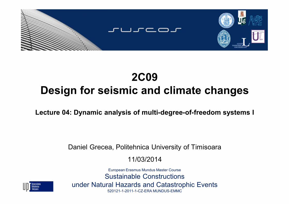
Multi degree of freedom systems

Multi degree of freedom systems Structure idealisation: elements interconnected at nodes Degrees of freedom: node displacements/rotations
– 3 DOF for two-dimensional frames – 6 DOF for three-dimensional frames
Forces applied at nodes
Multi degree of freedom systems
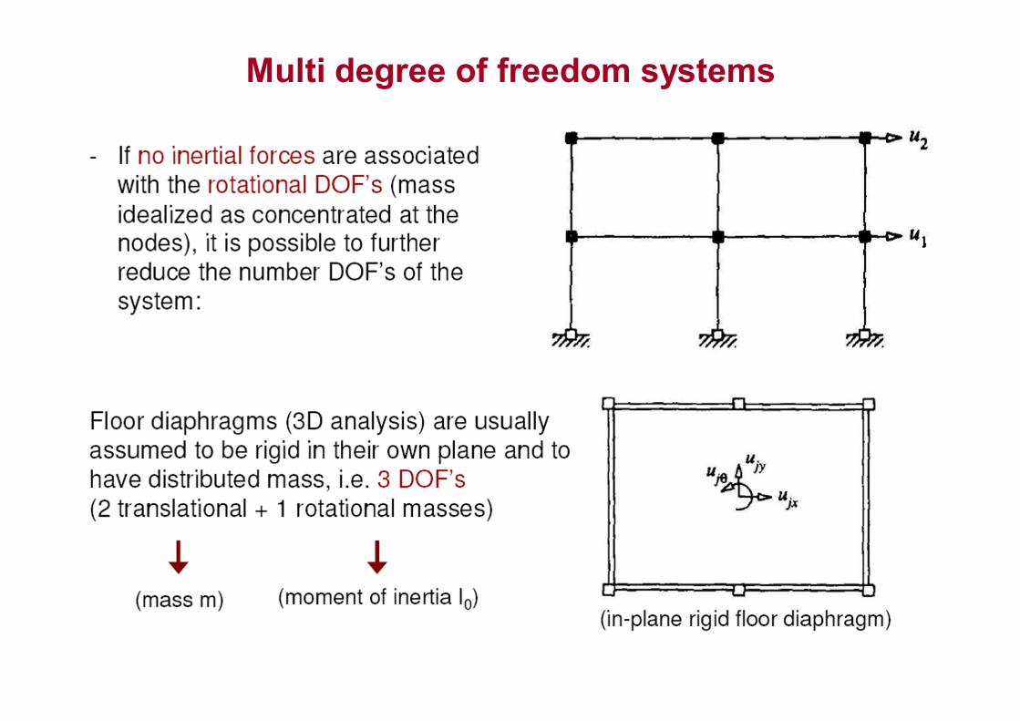
Equations of motion

Elastic forces Node displacements uj nodal forces fSj Linear systems: nodal forces determined based on
– superposition principle – stiffness coefficients
Stiffness coefficient kij is equal to the force along DOF i due to a unit displacement along DOF j
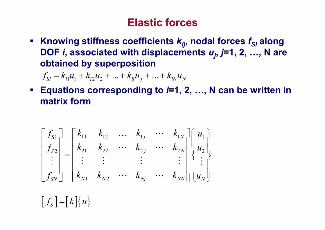
Elastic forces Knowing stiffness coefficients kij, nodal forces fSi along
DOF i, associated with displacements uj, j=1, 2, …, N are obtained by superposition
Equations corresponding to i=1, 2, …, N can be written in matrix form
1 1 2 2 ... ...Si i i ij j iN Nf k u k u k u k u
11 12 1 11 1
21 22 2 22 2
1 2
j NS
j NS
N N Nj NNSN N
k k k kf uk k k kf u
k k k kf u
Sf k u

Damping forces A unit velocity along DOF j, generates forces along
considered DOFs
Damping coefficient cij is the force along DOF i due to a unit velocity along DOF j

Damping forces Knowing damping coefficients cij, nodal forces fDi along
DOF i, associated to velocity j=1, 2, …, N are obtained by superposition
Equations corresponding to i=1, 2, …, N can be written in matrix form
ju
1 1 2 2 ... ...Di i i ij j iN Nf c u c u c u c u
11 12 1 11 1
21 22 2 22 2
1 2
j ND
j ND
N N Nj NNDN N
c c c cf uc c c cf u
c c c cf u
Df c u
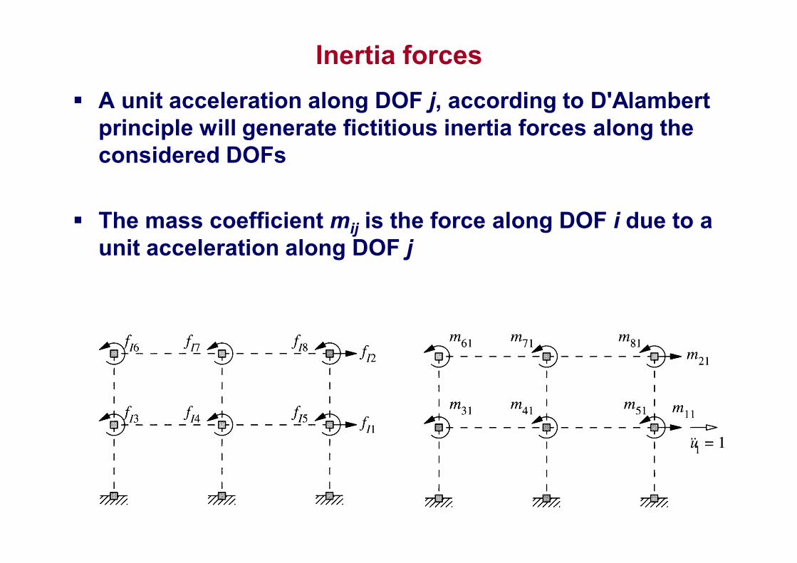
Inertia forces A unit acceleration along DOF j, according to D'Alambert
principle will generate fictitious inertia forces along the considered DOFs
The mass coefficient mij is the force along DOF i due to a unit acceleration along DOF j
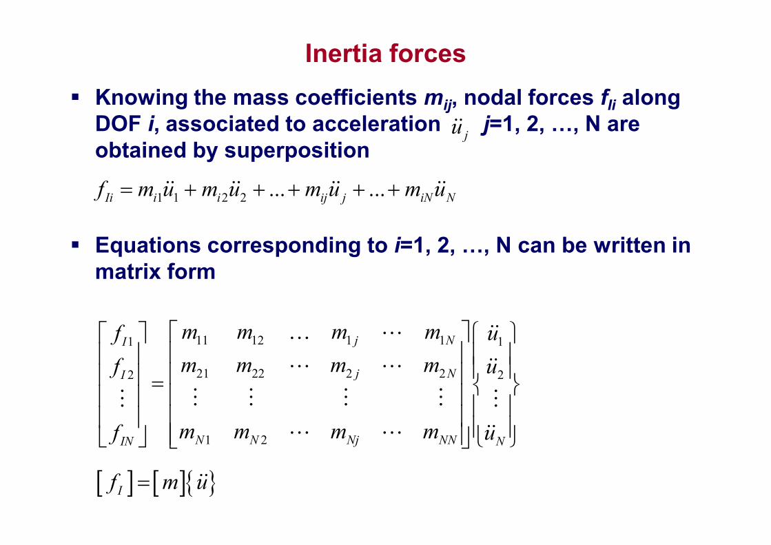
Inertia forces Knowing the mass coefficients mij, nodal forces fIi along
DOF i, associated to acceleration j=1, 2, …, N are obtained by superposition
Equations corresponding to i=1, 2, …, N can be written in matrix form
ju
1 1 2 2 ... ...Ii i i ij j iN Nf m u m u m u m u
11 12 1 11 1
21 22 2 22 2
1 2
j NI
j NI
N N Nj NNIN N
m m m mf um m m mf u
m m m mf u
If m u

Mass idealisation: 2D structures Generally mass is distributed through the structure In a simplified manner concentrated in nodes Rotational component: generally neglected Neglecting axial deformations of members masses can
be considered concentrated at the floor levels In general, for masses lumped in nodes, the mass matrix
is diagonal
0 0ij jj jm for i j and m m or
a b c
d e f
mb mamb mc
d e f
m1
2

Mass idealisation: 3D structures Multistorey three-dimensional structures: number of
elements in the mass matrix can be reduced due to floor diaphragm effect – infinite in-plane stiffness – flexible out of plane
Rigid floor diaphragms 3 DOFs defined at the center of mass: ux, uy, u
Flexible floor diaphragms masses should be assigned to each node , proportionally to their tributary area

Equation of motion: dynamic force Dynamic forces can be considered distributed to:
– stiffness component – damping component – mass component
Equation of motion:
p t Sf t Df t If t
I D Sf t f t f t p t
m u c u k u p t

Equation of motion: ground motion MDOF systems with al DOFs displacements in the same
direction with ground motion – ground displacement: ug – total displacement of mass mj: – relative displacement between mass and ground: uj
tju
1tj j gu t u t u t

Equation of motion: ground motion In case of ground motion dynamic forces
0p t
0I D Sf t f t f t
0tm u c u k u
1 gm u c u k u m u t
1tj j gu t u t u t
1eff gp t m u t
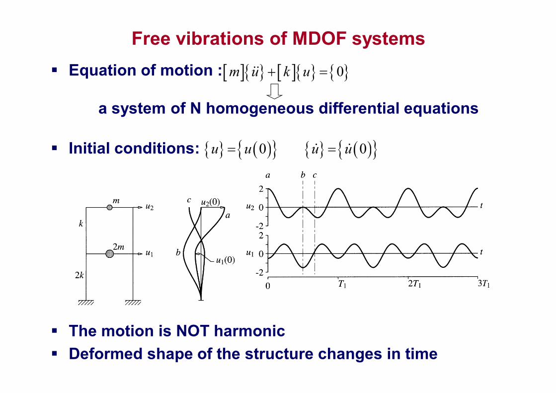
Free vibrations of MDOF systems Equation of motion :
a system of N homogeneous differential equations
Initial conditions:
The motion is NOT harmonic Deformed shape of the structure changes in time
0m u k u
0 0u u u u

Free vibrations of MDOF systems
0u u For an appropriate distribution of initial deformations:
Vibrations ARE harmonic Deformed shape does NOT change in time 1st Distribution 1st natural mode {}1
1st natural period T1
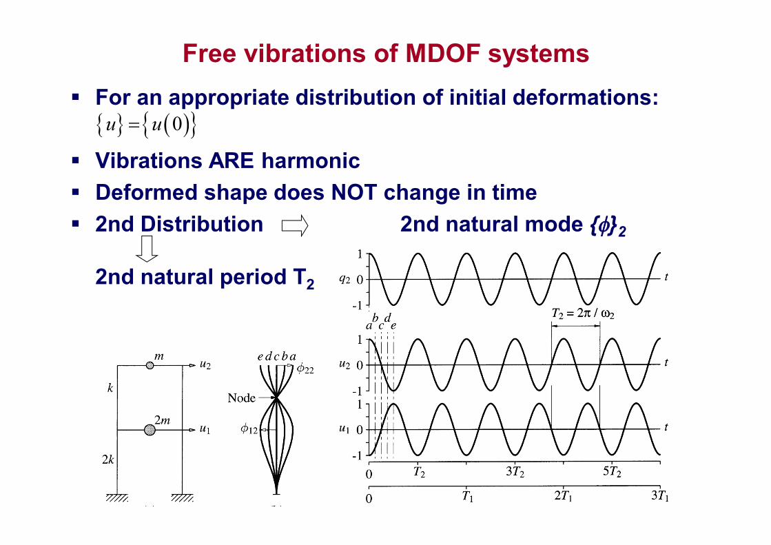
Free vibrations of MDOF systems
0u u For an appropriate distribution of initial deformations:
Vibrations ARE harmonic Deformed shape does NOT change in time 2nd Distribution 2nd natural mode {}2
2nd natural period T2

Natural modes of undamped MDOF systems Vibrations in n-th natural mode:
– deformed shape: {}n – time response:
qn(t)=0 or trivial solution non-trivial solution
eigenvalue problem determination of scalars n
and vectors {}n
n nnu t q t
cos sinn n n n nq t A t B t
cos sinn n n n nn nnu t A t B t q t 0m u k u
2 0n nn nm k q t
2nn n
k m 2 0n nk m
2det 0nk m
2 2 2cos sinn n n n n n n nn nnu t A t B t q t
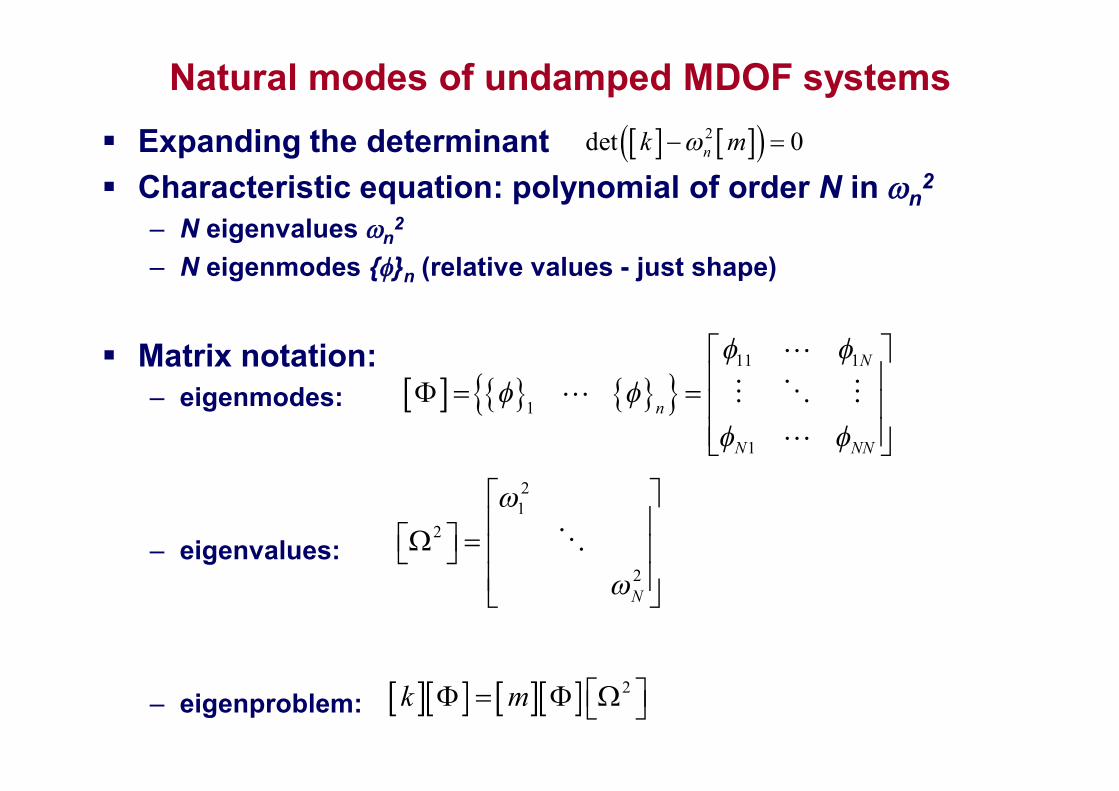
Natural modes of undamped MDOF systems Expanding the determinant Characteristic equation: polynomial of order N in n
2 – N eigenvalues n
2 – N eigenmodes {}n (relative values - just shape)
Matrix notation:
– eigenmodes:
– eigenvalues:
– eigenproblem:
2det 0nk m
11 1
1
1
N
n
N NN
21
2
2N
2k m

Orthogonality of natural modes Eigenproblem: Multiplying to the left by (rn):
Similarly:
Difference between (4.33) and (4.32):
For n2r
2, which for positive values implies nr:
orthogonality of natural modes Matrices M and K:
diagonal
2nn n
k m
Tr
2T Tnr n r nk m
2T Trn r n rk m
transpose 2T T
nn r n rk m (4.33)
(4.32)
2 2 0Tn r n rm
0T
n rm 0T
n rk (4.32)
T TK k M m
T Tn nn n n nK k M m 2
n n nK M

Normalisation of modes Natural modes: vectors for which only relative values are
known Normalisation of modes:
– setting the maximum value of a natural mode to unity – setting the value corresponding to a characteristic DOF to unity – normalisation of natural modes so that Mn are unity
(normalisation with respect to the [m] matrix) orthonormal natural modes
1 TTn n nM m m I
2 2 2TTn n n nn n
K k M K k

Modal expansion of displacements Any set of N independent vectors can be used to express
another vector of order N
qr - modal coordinates Multiplying both sides of (4.48) by
all terms are equal to zero, excepting those corresponding to r=n:
Modal coordinates can be determined:
1
N
rrr
u q q
(4.48)
T
n m
1
NT T
rn n rr
m u m q
T Tnn n nm u m q
T T
n nn T
nn n
m u m uq
Mm
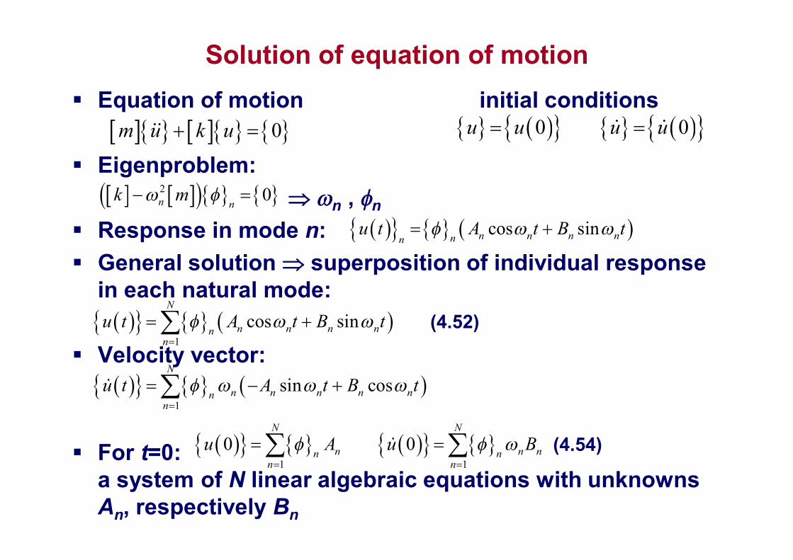
Solution of equation of motion Equation of motion initial conditions
Eigenproblem: n , n Response in mode n: General solution superposition of individual response
in each natural mode:
Velocity vector:
For t=0: a system of N linear algebraic equations with unknowns An, respectively Bn
0m u k u 0 0u u u u
cos sinn n n nnnu t A t B t
2 0n nk m
1
cos sinN
n n n nnn
u t A t B t
1
sin cosN
n n n n nnn
u t A t B t
1 1
0 0N N
n n nn nn n
u A u B
(4.54)
(4.52)

Solution of equation of motion Using modal expansion, vectors and can be
written as
where modal coordinates are given by:
Equations (4.54) and (4.55) are equivalent
Replacing these expressions in (4.52)
1 1
0 0 0 0N N
n nn nn n
u q u q
0u 0u
0 00 0
T T
n nn n
n n
m u m uq q
M M
(4.55)
0n nA q 0n n nB q
1
00 cos sin
Nn
n n nnn n
qu t q t t
1 1
0 0N N
n n nn nn n
u A u B
(4.54)

References / additional reading Anil Chopra, "Dynamics of Structures: Theory and
Applications to Earthquake Engineering", Prentice-Hall, Upper Saddle River, New Jersey, 2001.
Clough, R.W. şi Penzien, J. (2003). "Dynammics of structures", Third edition, Computers & Structures, Inc., Berkeley, USA