, I I

M I N I S T R Y O F S U P P L Y

AERONAUTICAL RESEARCH COUNCIL

REPORTS AND MEMORANDA

R. & M. No. 2918 (16,124)

A.R.C. Technical Report

The Calculation of the Pressure Distribution over the Surface of Two-dimensional and

Swept Wings with Symmetrical Aerofoil Sections

By "'-

J. WEBER, Dr. rer. nat.

t

Crown Copyright Reserved

LONDON : HER MAJESTY'S STATIONERY OFFICE

1956

PRICE 17S 6d NET

The the

Calculation of the Pressure Surface of Two°dimensional and Swept

with Symmetrical Aerofoil Sections By

J. WEBER, Dr. rer. nat.

COMMUNICATED BY THE PRINCIPAL DIRECTOR OF SCIENTIFIC RESEARCH (AIR),

MINISTRY OF SUPPLY

Distribution over Wings

Reports and Memoranda No. 2918 ?

July, 953

Summary.--A simple method is described for calculating the pressure distribution on the surface of a thick two- dimensional aerofoil section, at any incidence, in incompressible potential flow. The method has been proposed by F. Riegels and H. Wittich, Refs. 1 and 2. I t is particuIarly suitable for practical applications, since knowledge o_f the section ordinates only is required. This paper gives a complete derivation of the theory including a detailed discussion of the approximations made and their effect on the accuracy of the results. The pressure distributions calculated by the present method are identical wi th the exact values for aerofoils of elliptic cross-section, and the numerical values for Joukowsky aerofoils agree well with the exact solutions. Calculations for a typicM practical aerofoil show good agreement with the results from S. Goldstein's method, approximation III, Refs. 3 and 4.

The method is extended to sheared wings of infinite span and to the centre-section of swept wings, using tile solution for zero lift from Ref. 16 and the solution for the thin wing with lift from Refs. 10 and 17.

K_..

1. I~troduction.--The calculation of the pressure distribution over the surface of an aerofoil in inviscid flow is one of the classic problems of fluid motion theory. I t has regained importance in the design of swept-wing aircraft. A large number of calculation methods have been devised for two-dimensional aerofoils, and it is now possible to choose a method which is suitable for practical application and which is not likely to be superseded in the near future. Such a method must reduce the computational work involved to a few hours, so that the method should involve only the ordinates of the given aerofoil section. Experience has shown that the possibility of ever being able to provide a single series of aerofoil sections suitable for all purposes must be ruled out, at least for swept wings. Secondly, such a method must not make exclusive use of the method of conformal transformation because it must also be applicable to cases with essen- tially three-dimensional flow. Therefore the method of singularities should be used since it can be readily extended to three-dimensional flow, and the terms involved are open to some physical interpretation. This latter property is particularly helpful when approximate solutions including higher order terms must be found in those cases which have a complicated flow pa t t e rn ; experience has shown that the restriction to linearised theory in such cases does not often lead to adequate results.

The calculation method which provides the basis of the present paper is that of F. Riegels and H. Witt ich 1'2 (1942, 1948), which is closely related to those of S. Goldstein aa (1942, 1948) and B. Thwaites and E. J. Watson 5'6 (1945). The method for the two-dimensional unswept

j- R.A.E. Report Aero. 2497, received 9th September, 1953.

1 A

aerofoil is explained in sections 2 and 3. Conformal transformations are used only in deriving the methods for determining the distributions of singularities, from which the velocity distri- butions are calculated, and secondly, in determining a few exact solutions to check the accuracy of the method. By discussing the necessary assumptions and giving an estimate of the errors in the resulting velocity distribution.s, it is shown that the present method is suitable for practical application.

The method is then applied to the case of the sheared wing of infinite span in section 4 and to the centre section of swept wings of large span in section 5, both with and without lift. These cases may serve as the basis of a later extension of the method to wings of any given plan-form.

A numerical method to determine the occurring integrals as sums of products of the given section ordinates and fixed coefficients, and the evaluation of these coefficients, is explained in section 6. The calculation procedure is illustrated by a worked example in section 7.

The aim of sections 2 and 3 is to provide a complete derivation of the theory. Sections 4, 5 and 7 provide most of the details needed by the reader who is only interested in the application itself.

The investigation is restricted to wings with symmetrical aerofoil sections in incompressible flow. The question of what aerofoil shapes and pressure distributions may be desirable is not considered.

2. The Two-dimensional A erofoil at Zero L i f t . - -2 .1 . General Re la t ions . - -The aim of this and the following section is to calculate the pressure distribution on the surface of an unswept wing of infinite span. The flow around the aerofoil at incidence is here determined as the sum of two flows obtained by resolving the main stream into components parallel and normal to the chord-line. The aerofoil in a flow parallel to the chordline is treated in this section and the aerofoil in a flow normal to the chord-line is dealt with in section 3.

In any plane normal to the leading edge of the wing a system of rectangular co-ordinates x, z is used where the x-axis is along the chord with x = 0 at the leading edge (see Fig. 1). The co-ordinates are mad~ non-dimensional by reference to the wing chord, e. The shape of the aerofoil is assumed to be known :

z = z(x), 0 ~< x ~< 1 . . . . . . . . . . . . . . . (2-1)

The wing is placed in a uniform stream of velocity Vo, so that the velocity vector lies in the x, z-plane and is inclined at an angle ~ to the chord-line. The velocity Vo of the main stream is resolved into its components parallel and normal to the chord-line :

V,0 = V0 cos c~ . . . . . . . . . . . . . . . . (2-2)

V,0 = Vo sin ~ . . . . . . . . . . . . . . . . . (2-3)

First we deal with the aerofoil in the uniform stream V,0. This is the same problem as the aerofoil at zero lift, since we consider wings of symmetrical section shape only. The task is to determine a flow for which the given aerofoil section is a streamline, i.e., a flow for which the velocity component normal to the surface is zero. This is achieved by determining a distribution of singularities at the surface of the aerofoil which produces a velocity distribution at the surface whose normal component cancels the normal velocity component of the uniform stream Vxo.

At the surface of the aerofoil z(x), the uniform stream V,0 has tangential and normal components :

V~o = V.o ~ / { 1 + (dz/dx) 2} . . . . . . . . . . . . . . (2-4)

v.0(g /gx) v, 0 = - V { 1 + (az / e . )

2

(2-s)

To determine the required distribution of Singularities we make use of the method of conformal transformation. This is done only as an intermediate means of deriving a relation between the velocity distribution at the aerofoil surface and the section shape. I t will be shown that by introducing an approximation into this relation it is possible to determine the velocity distri- bution without actually performing the conformal transformation.

We introduce the complex variable ~ : e = x + i z

and transform the e-plane conformally into a ~* (= x* + iz*)-plane so that the part of the e-plane outside the contour z(x) is transformed into the ~*-plane outside a slit along the x*-axis. The determination of a singularity distribution in the ~-plane which produces a velocity distri- bution cancelling the normal velocity V,0 at the aerofoil surface is equivalent to the problem of determining a singularity distribution in the ~*-plane which cancels the normal velocity com- ponent V,0 :+ at the slit.

I t is known from the theory of conformal transformations that corresponding velocity com- ponents are related by the mapping ratio lde/de*[ :

. . . . . . . . . . . . . . . . . (2-6) V, oo* = V.o

The values of V,,o at corresponding points on the upper and lower surface of the slit are equal but of opposite sign. Such velocities can be cancelled by a source distribution at the slit• A con- tinuous distribution of infinite source lines normal to the x, z-plane produces a velocity field which is continuous everywhere except at the position of the sources. There the velocity com- ponent normal to the sources jumps by an amount proportional to the local strength q of the sources.

The required distribution of singularities is thus a source distribution, at the slit, of strength q(x*) = -- 2V,,o* . . . . . . . . . . . . . . . . . (2-7)

At the slit this source distribution produces the tangential velocity

f *'

1 q ( x ) . . , v,* (**-) = ~ x.~-- 7~.,~. . . . . . . . . . . . . . . (2-s)

which corresponds to the tangential velocity d V~ at the surface of the aerofoil in the original ~-plane :

= A V ,* . ~ . . . . . . . . . . . . . . . . . (2-9) A V,

At the surface of the aerofoil the mapping ratio is : ds ds dx

= dx* = dx" dx* where s denotes the length of arc along {he aerofoil surface. Hence,

d ~ = ~/{1 + (dz/dx)2} . . . . . . . (2-10) dx

4

d X ¢~ . . . . . .

From equations (2-5) to (2-10) we obtain the additional velocity which the singularities produce at the aerofoil :

• 7 V { 1 + (dz/dx) '} .,,..,, a e* .., x*(~) - x . '

- g { 1 + (gz/g~)~} 7 J \ ) T x . ,dx*' x * - x*'

_ V~o . 1 ( ~ ( x - x ' ) / ( x * - . * ' ) az , . ' . (2-11)

- - ~ / { 1 + (dz/dx) 2} = Jo (dx/dx.*), dx ' x - - x ' "" @ 0

3

O

Thus the total velocity at the surface of the aerofoil in the uniform stream V,0 is :

V(x, z) = V,o + ~ t7,

= ~ / { 1 ~ (~ /~x)~} 1 + g (d~/~-*) , ~ _ ~ _ x, . . . (2-12)

For an exact determination of the integral in this equation, the relation between x* and x is needed, i.e., the transformation would have to be carried out. However, the function

T(x, x') = (x - - x ' ) / (x '*- - x*') (dx/dx~.)~ . . . . . . . . . . . . . . . (2-13)

which gives the ratio between the distances of the pivotal point x and the variable point x' in the original plane ( x - x'), and in the transformed plane (x*--x*') , related to the local mapping ratio (dx/dx*) at the pivotal point does not differ much from unity. T(x, x') is equal uni ty for x' ---- x and we shall see in section 2.2 that the difference T(x, x') -- 1 is of the order of the thickness/chord ratio t/c. Since T(x, x') occurs only in the term which itself is of order t/c, an approximation for the velocity V(x, z) which is correct to at least the first order in t/c may be obtained by putt ing

T(x,.x') = 1 . . . . . . . . . . . . . . . . . . . . (2-14)

We shall discuss the accuracy of this approximation and its effect on the velocity distribution in detail in section 2.2.

With approximation (2-14) the velocity distribution (2-12) becomes:

y(x , ~) = ~ / { 1 + (d~/dx) 2} 1 + ~ ~x' x --~ x'J . . . . . . . . (2-1S)

This formula gives the required relation by which the velocity distribution may be ,determined from the given profile shape without performing the conformal transformation. A numerical method of calculating the integral

S ( l ) ( x ) = l j ' l o d Z dx' - - . o . . . . . . = dx' x -- x' . . . . . . . . (2-16)

for fixed points x, as sums of products of the ordinates z at the fixed points and certain coefficients which are independent of the section shape, is described in section 6.

Before we investigate the implications of approximation (2-14), let us discuss the result in equation (2-15) in view of our aim to extend the method from the two-dimensional aerofoil to three-dimensional problems. Equations (2-12) and (2-15) are obtained from a source distri- bution along the slit in the transformed plane. This corresponds to a source distribution on the surface of the aerofoil in the original plane. For three-dimensional problems, the use of such surface distributions is generally out of the question since they require very complicated calcula- tions. Since the calculations are considerably simpler when the source distributions are put on the chord-line, we interpret equation (2-15) in the following discussion as the result of a source distribution on the chord-line.

The condition thai the aerofoil surface is a streamline, i.e., that the total velocity component normal to the surface is zero, can be written in the form :

dz v /x , z) dx - - V.,o + v~(x, z) . . . . . . . . . . . . . . (2-17)

4

in linear theory this condition is approximated by t

d~ _ v~(., o) . . . . . . . . . ( 2 q 8 ) dx V~o . . . . . . . . .

which is equivalent to the following assumptions : (i) the velocity increment v, is small compared with V~0 ;

(it) the velocity v,(x, z) in the z-direction at the surface can be represented approximately by the velocity v / x , 0) in the z-direction on the chord-line.

This latter approximation considerably simplifies the problem of determining a source distri- bution which gives the required distribution of velocity v,. With a source distribution on the chord-line, the whole source distribution contributes to the velocity v, at a point on the surface, but the v~-velocity on the chordline is only dependent on the local source strength.

The required source distribution is :

dz (2 -29 ) q(x) = 2V.o d~ . . . . . . . . . . . . . . . . .

i .e. , the source strength is proportional to the local slope of the aerofoil contour.

The source distribution of the linear theory, as given by equation (2-19), satisfies the condition

(1 ~(x) d~ = o . . . . . . . . . . . . . . . . . . ( 2 -20 ) d 0

which is necessary to obtain a stagnation streamline which closes behind the source distribution, thus forming an aerofoil profile.

The source distribution of equation (2-29) also satisfies the condition that the total drag force D acting on the whole source distribution is zero. According to a theorem of A. Betz 7 (1932) about the tangential force acting on a source (which corresponds to the Kutta-Joukowsky theorem for the normal force acting on a vortex) the drag coefficient is : .,

D j l V ~ ( x ' ) q ( x ' ) d x ' . . . . . . . . . . . (2-21)

IJ v

With the approximation (i) made above: v~ (~ [7,0, i.e., V~ = V~0, it follows:

C~ = 0.

Linear theory also makes a third assumption :

(iii) the total velocity V(x , z) at the surface is represented approximately by the total V, velocity on the chord-line.

At the chord-line, the source distribution of equation (2-19) produces a velocity v~, along the chord, given by

/ ! I

v~(x, 0) -- V,o j I ~ dx #dz x dx'_ x ' . . . . . . . . . . . . . . (2-22)

The total velocity along the chord, V~, at the chord-line, which from linear theory is also the total velocity at the surface, is thus :

V / x , O) = V.o 1 + ~ dx' x - - x'

-- V,o [1 + S(1)(x)] . . . . . . . . . . . . . . . (2-23)

.5

A comparison of equations (2-15) and (2-23) gives the relation

v (x, o) V(x , z) = V ' { 1 + (dz/dx)~} " "" "" ": "" . . . . . (2-24)

We will see in section 2.2, from calculated examples, how much the velocity distribution given by linear theory is improved on multiplying by the factor 1/V'(1 if- (dz/dx)~}. The factor is important in the stagnation region, where the approximation (i) in equation (2-18) does not hold.

Later the rela~tion (2-24) between the velocity on the chord-line and the vel0eity at the surface will also be used as an approximation for the flow normal to the Chord-line of the aer0foil and in the three-dimensional case. I t can be interpreted by making use of the fact tha t the circulation around a distribution of singularities is independent of the path taken ' :

r = vtx, = v tx, 0/dx . . . . . . . . . . . . . (2-2s/

In the present case/~ = 0. Equation (2-24) now means that a corresponding relation is assumed to hold locally •

V(x , z) ds = V~(x, O) dx . . . . . . . . . . . . . . . . . (2-26)

2.2. E x a m p l e s and d iscuss ion o f the A c c u r a c y of the M e t h o d . - - I n deriving equation (2-15), the approximation of equation (2-14) was assumed to be admissible. We Shall now check the validity of this assumption for several aerofoil shapes and determine the error in the velocity distribution resulting from this approximation by comparison with exact results. For this purpose we have actually to perform the conformal transformation. We choose the two cases of, aerofoils of elliptic cross-section and Joukowsky aerofoils since for these the transformation into the slit is given by simple formulae. The ellipse and the Joukowsky profile are rather extreme cases, between which lie most practical aerofoil shapes. The usual type of aerofoil has its maximum thickness between 0.25c (Joukowsky profile) and 0.5c (ellipse) and has a finite trailing-edge angle t smaller than ~/2, whilst Joukowsky profile and ellipse give the two extreme values of 0 and z/2. The modern type aerofoils are usually of nearly elliptical shape ai: the nose an d u p to tl~e maximum thickness.

We begin with the elliptic aerofoil. The ellipse with axes c : 1 and t/c, and centre at the origin of the co-ordinate system in the C-plane, is transformed into a circle of radius r in the ¢~-plane by the transformation

R ~ ¢ = ¢~ + ¢~ . . . . . . . . . . . . . . . . . . .... (227)

with R = ~/{1 -- (t/c) 2 } 4

1 + (t/c) 4

The circle is then transformed into a slit in the ¢*-plane by the transformation

: * = ¢~ + ¢~ . . . . . . . . . . . . . . . . . (2-28)

~- For sections with finite trailing-edge angle < ~r/2 the source distribution q(x) of equation (2-19) has a finite strength at the trailing edge, which leads to a logarithmic infinity there of the integral S(l/(x), equation (2-16). Thisgives a velocity distribution with a logarithmic infinity at the trailing edge, whilst the exact value from potential theory is zero. Since the singulaxity is only logarithmic, its effect is negligible except for the very neighbourhood of the trailing edge where the flow conditions are considerably affected by the viscosity of the air anyhow.

We shall see later that, with the interpolation formula equation (6-4) used in the numerical method of section 6, profiles with a sharp trailing edge are replaced by profiles with a rounded trailing edge of very small radius of curvature, thus removing the singularity.

6

The circle in the ¢,-piane has the equa t ion :

~1 = r e ~ . . . . . . . . . . . . . . . . . . . (2-29)

Thus the real co-ord ina tes ~, ~1 = r cos v~, a n d ~*" for co r r e spond ing poin ts on the ellipse, the circle a n d ti le slit are g iven b y the relat ions~ •

~ = ( r + ~ ) c o s # = ½ c o s y ~ . . . . . . . . . . . . (2-30)

U* = 2r cos v ~ _ 1 -+- (t/c) cos v ~ . . . . . . . . . . . (2-31) 2

This gives the re la t ion

1 • ~* . . . . . . . . (2-32)

- - = 1 + (z/C) . . . . . . . .

Hence , : - - ' '

= (d#/d~*)~ = 1

a n d the re fo re the a p p r o x i m a t i o n (2-14) is s t r ic t ly t rue for the whole i n t e rva l of in tegra t ion , a n d for eve ry p ivo ta l po in t x. Thus equa t ion (2-15) gives the exac t ve loc i ty d i s t r ibu t ion for the aerofoils of el l ipt ic cross-sect ion of a n y t h i cknes s / cho rd rat io.

This resul t also m e a n s t h a t the th ree a p p r o x i m a t i o n s m a d e of l inear theory , descr ibed at the end of sec t ion 2.1, are ful ly co r rec ted in the case of the ellipse b y m u l t i p l y i n g V~(x, 0) b y the fac tor 1/~/{1 q- (dz/dx)2}, as in e q u a t i o n (2-24).

I t will p rove useful l a te r to k n o w the explici t fo rmula for the ve loc i ty d i s t r i bu t ion a long the ellii3se. Us ing the angle # as def ined b y equa t ion (2-19), the co-ord ina tes for the ellipse are, f rom equa t ion (2-27) :

1 + cos x = 2 . . . . . . . . . . . . . . . . (2-33)

, _t sin ~ . . . . . . . . . . . . . . . . . (2-34) Z = ~ c

The in tegra l S°)(x), equa t ion (2-16), can be ca lcu la ted explici t ly. I t is '

S(1)(x ) =-1 j dz dx' _2 dz dv a' dx' x - - x' ~ d#' cos tg' - - cos #

0

t 1 f l c o s ~ ' d ~ ' C 7c COS t9 ~ -- COS #'

t _ _ ° • • ° ° ° ° ° • ° ° ,

c

using the we l l -known re la t ion (see, e.g., H. Glauer t 8 (1948), p. 93) •

f l sin nv~ cos n# ' d~' = ~ . - - . . . . . cos ~' - - cos v~ sin v~

¢

(2-35)

(2-36)

i" The x-co-ordinate and the ~e-co-ordinate differ by an additive constant.

Equa t ion (2-35), together wi th equat ion (2-23), means tha t in l inear theory the velocity distri- but ion along the surface of an ellipse is constant and equal to V~0(1 + t/c). The exact value is, f rom equat ion (2-15) •

V~o V(x, z ) = ~/{1 + (dz/dx) ~} (1 + t/c) . . . . . . . . . . . . . (2.37)

Let us now consider the Joukowsky profile. The t ransformat ion R ~

= ~1 + ~ . . . . . . . . . . . . . . . . . . ( 2 . 3 s )

t ransforms the profile into a circle of radius r with the centre at ~1 = -- (r -- R) and the trans- formation

y~ ~*- = ~ + (r - R) + ~ + (r - R) . . . . . . . . . . (2-39)

t ransforms the circle into a slit. The difference r R is related to the thickness/chord ratio. We introduce the parameter e by •

r = (1 + s)R . . . . . . . . . . . . . . . . . (2.40) I t will be shown later tha t in linear theory :

4 t s -- 3V'3 c . . . . . . . . . . . . . . . . (2-41)

The relation between the real co-ordinates ~ and ~* of corresponding po in t s along the aerofoil and the slit can be obta ined from equations (2-38) to (2-40)~. We have •

~ e , = 2($~ + r - R) . . . . . . . . . . . . . . (2-42)

= ~ + r 2 - ( ~ l + r - R ) ~ + ~ 2 . . . . . . . . . . (2-43)

with

R 2

1 I . . . . . . ,244, 1 -[-2e + 2 e 2 - e ~

-- 2(1 + e) ~< ~ ~< 2(1 + e) . . . . . . . . . . (2-45)

- - 2 1 + 1 + 2 % / ~ < R ~<2 . . . . . . . . . . . (2-46)

Using equat ion (2-44) the function T(x, x') can be calculated numerically. This has been done for profiles of 10 per cent and 20 per cent thickness/chord ratio. The results are p lo t ted in Fig. 2. An approximate formula for T(x, x') can be obta ined by expressing ~/R from equat ion (2-44) as a power series of e and neglecting high order terms :

R - - R ( 1 - - ~) + ~ - - 2~

l . d~.~ = 1 -- e - / s R

1" The ~-co-ordinates used here differ from the x-co-ordinates used otherwise in this note by additive constants.

8

we get

r (x , x') = T(~, ~') = (~/R - - ~ ' /R) / (~*/R-- ~*'/R) (d~/a~*),,

Finally, in x-co-ordinates referred to the chord :

T(x, x') = 1 -- 2s(x* -- x*') . . . . . . . . . . . . . . (2-47)

using the relation

( . . . . . . . . c = 4 R 1 + 1 -}-2e . . . . . .

between the chord c of the aerofoil and the radius R, which follows from equation (2-46 i Equa t ion (2-47) gives approximations for the lower and upper limits between which T(x, x') varies :

1 - - 2e <~ T(x,x') <~ 1 + 2e.

Fig. 2 and equation (2-47) show that the maximum error made in the integrand of equation (2-12) when using the approximation T(x, x') = 1 is proportional to tic. At the pivotal point the approximation is correct and the difference IT(x, x') -- 11 becomes greater the further the varying point moves away from the pivotal point. This means that the contribution of the sources and sinks further away from the pivotal point is less accurately .taken into account than the effect of the nearby sources. I t will be shown later that the integral S(ll(x), equation (2-16), is of the order tic (see equation (2-35) for elliptic aerofoils). The difference between the velocities calculated by the exact equation (2-12), and the approximation (2--15), is therefore of higher order than tic.

In the following, we shall see that the error in the velocity distribution due to the approxima- tion T(x, x') = 1 is considerably less than the error in the local values of the integrand. To determine the error in the velocity distribution we calculate the exact velocity distribution from the conformal transformation and compare it with the velocity distribution as given by equation (2--15). The latter is calculated by the numerical method to be described in section 6.

For the present purpose we do not determine the velocity distribution at the aerofoil by means of a source-sink distribution as in section 2, but directly from the transformation. Since the total velocity along the slit is equal to V, 0 the velocity at the aerofoil is :

V d¢+J V = ,0 ~ •

The mapping ratio is given by the transformation, equations (2-38) and (2-39) :

Id**/d¢ll v = V,o I d ¢ l d ¢ l l

r~ R ) ~ 1 - -

= v~0 (¢1 + r -

1 R~

The circle in the el-plane which corresponds to the aerofoil has the equation

~i = R1 d~' . . . . . . . . . . . . . .

9

(2-49)

(2-50)

with = RE /{ 1 + + cos cos (2-51)

From equations (2-40), (2-49) and (2-50), we obtain for the exact velocity distribution •

Equations (2-43), (2-48) and (2-50) give the relation between the chordwise position ~ on the aerofoil and the angle #~

c -- 4(1 + 2e ~- e ~) -t- cos ~ . . . . . . . . . . . (2-53)

When calculating the approximate velocity distribution from equation (2-15), we need the section ordinates. These are known from the transformation. Equations (2-38), (2-48) and (2-50) give"

: c - 4(1 + 2~ + ~ ) R " " "

For the rather extreme case of a 20 per cent thick Joukowsky aerofoil, the exact velocity distribution has been calculated numerically using equations (2-51) to (2-53). T h e results are given in column (a) of Table 1. The value e .= 0. 1833 was determined from equation (2-54). The values of ~9.~ were chosen so as to give the x/c-values used in the numerical method of section 6. for N = 162 Table 1 also gives in column (b) the results of the approximate method, equation (2-15). The agreement is very good. This comparison shows that the error made in the approxi- mation T(x, x') = 1 (see Fig. 2) does not involve any serious error in the velocity distribution.

Similar good agreement between the approximate velocity distribution calculated by the methods of conformal transformation (using the approximation I I I of S. Goldstein a (1942) and the vel0city distribution calculated from equation (2-15) has been obtained for the 10 per cent thick RAE aerofoil sections 100 to 104 (see R. C. Pankhurst and H. B. Squire 9 (1950)). An example is shown in Fig. 3. These results prove that no further refinement of the present method is necessary.

To allow a further judgment of the accuracy of the present method, it is desirable to have another illustration of the effect of second-order terms in t/c on the velocity distribution. The Joukowsky profile gives a simple example for this. There are several possibilities of neglecting higher order terms, e.g., in approximating the section shape, or in calculating the velocity distribution for the exact or the approximate section shape.

In obtaining the profile shape of the Joukowsky profile from the conformal transformation, second-order terms in e are often neglected. This leads to a profile tha t is different from the exact one given by equations (2-51), (2-53) and (2-54). The approximate shape is :

R1 = R[1 + e -- e cos ~1] . . . . . . . . . . . . . . (2-55)

~ - - ½cos ~ . . . . . . . . . . . . . . . . . . (2-56) 6

Z - = le(1 -- cos ~) sin ~ . . . . . . . . . . . . . . . (2-57) C

10

T h e thickness t of the approximate profile can be determined by differentiating equation (2-57) with respect to ~1. z(~l) has its maximum value for @1 = 120 deg. Inserting this value into equation (2-57) we obtain

max a v ' a t - - 2 - " - - e, c c 4

i.e., equation (2-41). For the 20 per cent thick Joukowsky profile, equation (2-41) gives S - : 0-1538, whilst the exact value from equation (2-54) is 0. 1833.

The velocity distribution for the approximate section shape of equation (2-56) and (2-57) is from linear theory, equation (2-23) :

V = V~0[1 + ~ -- 2e cos ~i] . . . . . . . . . . . . (2-58) since

I. . . . . . .

using equation (2-36). The same result is obtained when all higher order terms in e are neglected in equation (2-52) for the exact velocity distribution. The velocity distribution of the linear theory calculated from equation (2-58) for the 20 per cent thick Joukowsky profile is also given in Table 1, column (c). I t is calculated for the e-value resulting from linear theory. A comparison with the exact values in column (a) shows that the higher order terms have a considerable effect near the nose.

Mult iplying the velocity from equation (2-58) by the factor 1/1/{1 + (dz/dx)"}, we obtain for the approximate section shape, the velocity distribution corresponding to equation (2-15)!

(1 + e) sin v~ -- e sin 2~1 . . . . . (2-60) V = V~o ~,/{sin2 ~1 + e2(cos 2v~ -- cos v~l) ~} " " "

Calculated values are given in column (d) of Table 1. A comparison of columns (c) and (d) shows the effect of the correction factor l/w/{1 + (dz/dx)~}. The difference between column (b) and (d) is due to the difference between the exact and the approximate section shapes.

Another approximation for the velocity distribution is obtained by retaining the terms of the: lowest order in e in the numerator and denominator of the formula for the exact velocity distribution, equation (2-52):

(1 + s) sin v~ -- s sin 201 . . . . . . (2-61) v = _V o V{sin + - c o s . . . .

Equation (2-61) leads, of course, to two different values for the velocity distribution depending on which value of e is used.

The e value of the approximate section shape, equation (2241), gives the values of column (e), the exact e those of column ( f ) . The results obtained from equation (2-61) show much larger variations from the exact values of column (a) than do the approximate values of column (b) calculated by the present method. This confirms that equation (2-15) gives an approximation for the velocity distribution at the surface of a symmetrical aerofoil at zero lift which takes the higher order terms well into account.

'31 The Two-dimensio~al Aerofoil at Imidence.--3.1. Ge~eral Rdat iom.--As the next step towards our aim of calculating the velocity distribution on the surface of a two-dimensional wing at any given incidence we consider the aerofoil in a uniform stream V,o normal to the chordline.

• :First we recapitulate the theory of the thin aerofoil, i.e., the flat plate, which is an obstacle in the flow V,o but not in the flow V~o. I n the following we require the velocity field in the neighbourhood of the plate I as well as along it. This is easily determined b y means of the complex

11

potent ia l funct ion for the flow around the plate. To obtain the potent ia l funct ion we t rans form the plate -- ½ ~< ~ ~< ½ in the C-plane into a circle in the ¢1-plane •

R~ ¢ = ¢1 + ~-~, 2? = I . . . . . . . . . . . . . . (3 -a)

and the circle into a vert ical slit in the ¢~-plane • R2

~ = ¢ 1 - ~ . . . . . . . . . . . . . . . . ( a - 2 )

Combining equat ions (3-1) and (3-2) •

~ = V ( ~ ~ - 4R~) = ~ / ( ~ - k) . . . . . . . . . . . . . ( 3 - 3 ) The uniform stream, in the ¢2-plane, which is not dis turbed by the vert ical plate, has the complex potent ia l funct ion •

F ( ¢ ~ ) = ¢ + i~p = - - i v y & . . . . . . . . . . . . . . . (3-4) I t follows from equat ions (3-3) and (3-4) tha t the function

2%(¢) = - ~V~o(~ ~ - ~);~ . . . . . . . . . . . . . . ( 3 - s )

represents one possible flow around the horizontal plate. The veloci ty field of this flow is given by the relat ion •

d e - v , 1 - c v z l = - iV~o ~ / ( ¢ ~ _ I )

The veloci ty is infinite at both ends of the plate. Physical reasons do not allow an infinite velocity at the t rai l ing edge in viscous flow. To represent the l imit ing case of vanishing viscosity, we require a flow pa t te rn which fulfils the Ku t t a - Joukowsky condit ion of smooth outflow at the t rai l ing edge.

A flow wi th finite veloci ty at the trai l ing edge, ¢ = >1 is obtained by adding a flow wi th circula- t ion around the plate, for which the plate is a streamline. Such a flow is obtained from the flow around the circle and the t ransformat ion of the circle into the plate, equat ion (3-1) •

F~ = i ~ in ¢1

. F = ~ ~ In [½{¢ -t- ~/(¢~ - - I ) } ] . . . . . . . . . . . . (3 -6)

The potent ia l for the general flow around the plate is then

- ~vz0v~(¢ ~ - I) + ¢ f 7 in [~{¢ + x / ( ¢ ~ - I ) }~ F F1 + F~

and the veloci ty field is given by

d F ~ I ~ 1 d~ -- V~ -- i v y = -- iVy0 ~/(¢~ _ I) + ~ 2~ x/(¢ ~ -- I) . . . . (3-7)

The veloci ty is zero at ¢ = ½ if r V,0

2= 2 so t h a t

V e - - ¢ V , = ± V~o ½ + . . . . . . . . .

At the plate the veloci ty in the usual co-ordinate sys tem is '

the posit ive sign holds for the upper surface and the negat ive sign for the lower surface.

12

The vetocity component normal to the plate is zero, since the plate is a streamline. Tile tangential velocity is of opposite sign on upper and lower surface. Such a flow pat tern can be represented by a distribution of vortices (i.e., infinite vortex lines normal to the x-z plane) at the position of the plate, the strength ~, of which is equal to the jump in the tangential velocity when going from the upper surface to the lowersurface.

~(x) = v ~ s - v~s . . . . . . . . . . . . . . . . . (3-1o) The flow around the plate is thus equal to the flow obtained by superposing a vortex distri-

bution at the plate, of strength

~(x)

on the uniform stream V,0. This vortex distribution produces a v,-component at the plate

v, (x, 0) = -- 2~ r(x') x -- x - - - ~ . . . . . . . . . . . . . . (3-12)

which for ),(x) of equation (3-11) is constant along the plate, and equal to -- V,0.

We will now deal with the flow around a thick aerofoil. Again, our aim is to represent the aerofoil by a distribution of singularities which produces at the surface of the aerofoil a normal velocity distribution cancelling the normal velocity component of the uniform stream V~0. To determine the required singularities we might again t ry to use the eonformal transformation of the ~-plane into the ~*-plane, which transforms the aerofoil contour into a slit. I t will be shown in section 3.2 that the velocity component V,0* normal to the slit, which corresponds to the normal component V,,0 of the uniform stream V,0 in the Z-plane, is, for a general aerofoil, not constant along the slit. This means that we cannot use the vortex distribution ~(x) of the flat plate, given in equation (3-11). Furthermore, a vortex distribution along the slit corresponds to a vortex distribution on the surface of the thick aerofoil. To allow a simple extension of the method for the two-dimensional aerofoil to three-dimensional problems, we wish to represent the aerofoil by singularities on the chord-line.

We shall determine the vortex distribution which represents the thick aerofoil as th6 distri- bution (3-11) for the flat plate and an additive term A y(x) which depends on the section shape. We start, therefore, with the vortex distribution of equation (3-11) on the chord-line and calculate the velocity induced by it on the surface of the thick aerofoil. We obtain an approxi- mation for the velocity field in the neighbourhood of the chord-line by expanding the right-hand side of equation (3-8) into a power series with respect to z and neglecting all higher order terms :

v ~ - iv , = + v,0 . / ~ I - - ~ 2 _ ~ ± iz \ ~ k (-~ + e)2 + ~ J

= + V,o 1 . . . . ( 3 - 1 3 ) ~ / i I + ~J (~ + ~ ) ~ / ( ~ - ~=) ..

In the usual co-ordinate system the total V=-velocity is : Z

V,(x, z) = V=o + v,(x, z) = V=ox~/{ 1 _ (1 -- 2x) ~} . . . . . . . . . (3-14)

Equat ion (3-13) implies that for the vortex distribution of the flat plate the approximation

v.(x, z) = v.(x, o) = ± ~(x) 2 ""

is correct, if we consider only linear terms in z. ~(x)

v /x , z) = v~(~, o) = ± 2

for source distributions.)

. . . . . . . . . . . . (3 -15)

(This relation corresponds to the approximation

13

The condition that the aerofoil surface is a streamline can be written in the form (as in equation (2-17))"

2

dz V / x , z) dx v~(x, z)

Using the approximation (3-15) for any vortex distribution this condition can be mated by •

V,(x, z) = r(x) dz . 2 d ~ . . . . . . . . . . . . . . . . ( 3 - 1 ~ )

approxi-

A comparison of the required Vzvelocity, equation (3-16), with the V,-velocity produced by the vortex distribution of the flat plate, equation (3-14), shows that we need a correction Z~,(x) to the vortex distribution (3-11)"

2 V ~ 0 % / ~ t + A ~ ( x ) , . . . . . . . . . . . . (3-17)

n ~ ~

~(x)=

which produces the additional velocity component dr,, where

( 3 - 1 s )

With It is, of course, again desirable to take for A r (x) a vortex distribution on the chord-line. A) , (x ) being only a correction term, some further approximations in equation (3-18) are per 7 missible. First, we make the approximation

i .e . , we determine a vortex distribution Ar(x) which produces the required Av,-velocity on the chord~line. Secondly, we make the approximation

v 0/fl -2\ since A~(x) is small compared with the basic term 2V~0~/{(1 -- x)/x}. We will see later that the ratio between the two terms is of the order t/c. We obtain thus from equations (3-12) and (3-18) for At(x) the equation :

1 fro A , ( x , ) d x ' 2~ x - - x ~ - - A v / x , O)

(3-19) - ) = L o , ~ / ~ ,~ j k ~ t ~ 1 - (1 - 2 ~ ) ~ "

To solve this equation we treat the general problem of determining a vortex distribution along a flat plate which produces a velocity distribution with given components normal to the plate. For this purpose we transform the slit -- ½ ~< ~ ~< ½ in the ~-plane into a circle in the ¢l-plane by equation (3-1), and make use of the fact that in potential flow with given normal velocity v,~ (1) at the circle, the tangential velocity vt (1) is determined by the Poisson integral:

J? vt(1) = -- 2~1 cot #1' --2 e~ dO~' + const . . . . . . . . . (3-20)

The normal velocity v,/1/in the ¢~-plane is determined by the A v, velocity in the C-plane :

v,~ (1~ = Av~ = 2 sin %~1 • V ; , . . . . . . . . . . . .

14

where ~1 = } e ~' . . . .

represents the circle. From the relations

d v~ : - - Vt O) d~l I Vt(1)

and

it follows tha t

Since

A y = 2Ave

1 1 A v, sin v~ ' cot - -

Ay -- sin ~'~1 g 0

v a l ' - - t 9 1 - / c o n s t

~- d'G sin G

(3-22)

cot ~1 ! -- ~i sin G ' + sin G 2 COS v~l - - COS t~ 1'

we obtain, for symmetr ica l aerofoils for which AG(G) = Av=(2z~ - - G ) :

sin G ' d G ' const Ay 2 1 sin G ' sin G cos G -- cos G ' sin G

The angle G can be replaced by the chordwise co-ordinate 2. F rom equations (3-1) and (3-22) :

5 = ½ cos ~ so tha t

- - • ~¢/{1 - - (22) 2} v= V / { 1 - - (25') ~} ~ _ 5' ,V/{1 - - ( 2 5 ) 2 } "

We are again only interested in a flow with finite velocity at the trailing edge, which means dy(5 = ½) = 0. This condit ion determines the value of the constant. Thus

" f+' I ' ' t - ~v,(5') ~/<1 - ( 2 5 ' ) =} ~ 2' 1 _ ~ / {1 - ( 2 5 ) =} -~ - ~ 2' at '

which can be wri t ten as

2 1 ~+~ - - - dv=(5') ~/{1 - - (25 ' ) =} 1 -- 22 dU Ay J 1 - - 2 2 ' 2 - - 2 ' x / < l - ( 2 5 ) =} -~

2 - - 22 A v / U ) + - ; + ~ - 2 5 ' j 5 - 5'"

The vortex distr ibution which produces a given A v= is therefore given by the equat ion :

" d y ( x ) 2 z Av=(* x - - x ' . . . .

in the usual co-ordinate system. Thus the addit ional vor tex distr ibution is, from equat ions (3-19) and (3-23):

x Jd0 dxx' 1 - - ( 1 - - 2x') x - - x " '

15

So tha t the total vortex distribution which represents a thick aerofoil is :

x ; ~ 1 - ( I - 2x') x - ~ ' J " 3-25)

From the known vortex distribution we determine the velocity at the surface of the thick aerofoil by using the approximate relation (2-24) or (2-26) between the velocity on the chord-line and the velocity on the surface. The total velocity on the chord-line is :

V, (x , o) = :k b , ( x ) .

Hence, the velocity on the aerofoil, in a uniform stream V,0 normal to its chord-line, is :

V(x, z) ----- ± ~/{1 + (dz/dx) ~} 1 + • dx-x' 1 - - (1 -- 2x')~] x - x 'J" "" (3-26)

The accuracy of this approximate solution is discussed in section 3.2.

Having calculated the velocity distributions along the aerofoil produced by uniform streams parallel and normal to the chord-line, we can now determine the total velocity on the surface of a symmetrical aerofoil in a uniform stream V0 inclined at an angle c~ to the chord-line. Since the velocity components of the main flow parallel and normal to the chord-line are

V~o = Vo cos

V,~ = V0 s in c~

we obtain by combining the results of equations (2-15) and (3-26) :

V(x,z) = ~ / { l + ( d z / d x ) ~ cos~ 1 ~-~- d x ' x - - x '

flE ± sinc~ J { l - - X } [ l + -I dz 2z(x') ] dx' l~ x ~ 1 -- (1 -- 2x')2J x - ~' j j (3-27)

The positive sign holds for the upper surface, the negative sign for the lower surface.

For convenience, we use the notation of equation (2-16)

S,l,(x ) = _ l f }dz dx' ~z d x ' :~ - - x ' '

and

d z Sc21(x) _ dx' . . (3-2s)

s~,@) =

The equation for the

v(~ , z) Vo

dxx' 1 - - ( 1 - - 2x') x - - x " 0

velocity distribution then reads :

cos o'.[1 + S(~)(x)] 4- sin oc [1 :g

16

+ Sl~/(x)]

(3-29)

(3-30)

A method for calculating the functions S(1)(~;), S(2)(X) and S(a)(x) numerically at certain fixed points x, along the chord, when the ordinates of the aerofoil section at the fixed points x, are given, is described in section 6. The functions are approximated by sums of products of the ordinates and certain coefficients, which are independent of the section shape •

N - ~ (3-31) S m ( x , ) = ~ s ,}~) z,, . . . . . . . . . . . . . . . .

/ t = l

N--l . (3-32)

N - , . / e . . . . ( 3 - 3 3 ) S (~)(x,) = y. s#p z, + s'd~) ~ 2-c . . . . . . . .

l*=l

where p is the radius of curvature at the leading edge. The coefficients s~}% %m), %}a) are determined in section 6 and calculated values are given in Tables 3 to 12. In most cases it is advisable to use Tables 7 to 9, taking 16 points along the chord.

Using Bernoulli's equation for incompressible flow the pressure coefficient along the surface of a two-dimensional aerofoil at incidence cc is •

C~ = -- o _-- 1 -- p

?{, - {cos ct 11 q- S(*)(x)] 4- sin m V [1 -J- Sm)(x)]} 2 . . (a-a4)

1 + [S~=~(x)] 2

At high incidence the pressure distribution On the upper surface has a high suction peak near the nose of the aerofoil and changes rapidly along the chord. In this case it is advisable, for practical calculations, to write equation (3-34) in the following form •

C~ : 1 -- {cos ~[I + S(*)(x)] -V/x 4- sin c~ ~/(I -- x)[l + S(a)(x)]} ~ .. (s-as)

The chordwise load distribution, i.e., the difference between the pressure coefficients on the upper and lower surface of the aerofoil is, from equation (3-34) •

A Up ---- Cpus -- Cp~s

/ ( 1 - ~][1 + s(~(~)l[1 + s<~(x)l . . (3-36) = - 4 c o s sin + -

factor I1 + S/*~(x)][1 + S/~(x)] gives the correction to the flat-plate distribution due to The

the non-zero thickness of the aerofoil. The term [1 q-S(1)(x)] takes into account the fact that the vortices are put into a flow with the velocity Vo[1 + Sm(x)], instead of Vo as for the thin wing. The term [1 Jr SIa)(x)] takes into account the fact that the vortex distribution

1 for the thick wing- differs from that for the thin wing. The term i q- [S(~/(x)] 2 is the usual

correction term to allow for the difference between the velocities at the chord-line and on the surface. The first two terms increase the load over the forward part of the aerofoil and decrease it over the rear part. The third term reduces the infinite suction at the leading edge of the thin wing to finite values.

17

From the load distribution, the coefficients of the normal force and the pitching moment can be obtained by integration •

f' cN = - ~ c , d~ = - 2 ~ c , ~ / ~ d r % . . . . . . . . . . ( 3 - 3 7 /

o 0

c , , , = ~ c , ( x - 0.25) dx = 2 ~ C , ( x - 0 .25)Vx d~/x . . . . . (3-38) 0 • 0

The lift coefficient and the drag coefficient are related to the coefficients of normal force and tangential force by the equations •

CL = CN cos e -- C,c sin ~. . . . . . . . . . . . . . . (3-39)

Ca = CN sin ~, + Cr cos ~ . . . . . . . . . . . . . . . (3-40)

Since the drag in potential flow is zero,

i.e., Ca = 0 . . . . . . . . . . . . . . . . . . . (3_41) we have"

Cr = -- tan ~ C~ . . . . . . . . . . . . . . . . . (3-42)

C~ CL = • . . . . . . . . . . . . . . . . . . (3-43)

CO S 0~

3.2. Examples and Discussion of the Accuracy of the Method.--To check the validity of tile approximations made in deriving equation (3-26) for the velocity distribution along the aerofoil in a uniform stream normal to its chord-line, we again calculate the exact distributions for aerofoils of elliptic cross-section and for Joukowsky profiles, and compare them with the approximate results.

The exact velocity distribution can be determined from the velocity distribution of the flat plate, equation (3-8), using the transformations given in equations (2-27) and (2-28) which transform the flat plate in the ~*-plane into an ellipse in the C-plane. To the velocity distribution of the flat plate

v(x,, o )= + V:o ~/ Lc.,i 2 + 7~

corresponds the velocity along the ellipse '

• /¢c*-/2- ~*'} d~ V(x, z ) = ::j:: V~o 4 t ~ + ~ . . . . . . . . . . . . . (3-44)

Thus, using equations (2-10) and (2-32), we obtain, for the exact velocity along the surface of elliptical aerofoils in a flow normal to the chord the equation

" x ~¢/{1 -]-(dz/dx) 2} . . . . . . . . . ( 3 - 4 5 )

To determine the approximate distribution from equation (3--26), we calculate the t~rm S<*)(x), equation (3-29). I t follows from equations (2-16), (2-33), (2-34), (2-35), (2-36), (3-.9), that •

s<~,(x) _ s ( , , (x ) _ _ 2 ( 1 z (x ' ) u x '

J0 1 -- (1 -- 2x')~x -- x'

=t /c - - -1 t j l . _ dO" :7l: C C O S ~9' - - C O S ~9 ' t

= l / C . . . . . . . . .

18

., (3-46)

This means that equation (3-26) gives the velocity distribution of equation (3-45). In the case of elliptic aerofoils equation (3-26) is therefore exact. I t has already been shown in section 2.2 that equation (2-15) gives the exact velocity distribution for a flow parallel to the chord. These two results mean that equations (3-27) or (3-30) give the exact distribution for elliptical aerofoils at any incidence ~.

The pressure coefficient for aerofoils of elliptical cross-section at any incidence c~ to the uniform stream V0 is therefore •

( ,,.'2- )

• 1 - - X " 2

{,o, + ,m ; )} /- . . . . . . (3-47)

The chordwise load distribution is

1 + L c ) 1 - - (1 2x) 2

To obtain the lift coefficient we integrate the load distribution •

with

C~v= --A@dx=4cos~sino'. 1 + . J 1

J

j _ f i ~ / Q l - * ) * *° x E1 - ( t / c )2] (* - .2 ) + ~(qc)2 g x .

The integral J can be written in the form

19

Using the relations

d x - -

we obtain

and finally,

d N ~ - - 7t

f o r a < 0 o r a > 1

J - 2 1 + t/c

CN = 23(1 4- t/c) cos e sin

Cz = 23(1 + t/c) sin e . . . . . . . . . . . . . . . (3-49)

The last relation states that, for the same incidence, a greater lift is acting on the thick aerofoil than on the thin one. The same is true for ordinary aerofoils with sharp trailing edge. For these the correction factor to the lift of the thin aerofoil can be approximated by 1 @ 0-8 tic :

CL = 2~(1 + 0.8 t/c) sin ~ . . . . . . . . . . . . . (3-50)

To make a comparison between the exact velocity distribution and the approximation of equation (3-26), for the Joukowsky profile, we first determine the exact distribution again using equat ion (3-44). The mapping ratio Id¢*/d¢ I has been determined from the transformations (2-38) and (2-39) in equations (2-49) to (2-52). It follows from equations (2-40), (2-42), (2-45), (2-50) that

The exact velocity distribution along the Joukowsky profile in a uniform stream normal to its chord-line is therefore ;

g ~ Yz0

1 - e o s

, / i R. j , /( [,1 + 2 ~ + ~ - c o s ~ s i n ~ + L 2R~/R 1

. . ( 3 - 5 1 )

Some values calculated for the 20 per cent thick aerofoil are given in column (a) of Table 2.

Values for the approximate velocity distribution of the present method, equation (3-26), have been calculated by the numerical method of section 6, using the ordinates of the exact section shape given by equations (2-53) and (2-54). The comparison of the approximate values in column (b) with the exact values in column (a) shows good agreement, especially in the front part of the aerofoil. This implies that equations (3-34) and (3-35) give a good approximation to the suction peak.

Similar agreement is obtained for the 10 per cent thick sections RAE 100 to 104 between the results of the present method, equation (3-36), and the approximation I I I of the method by S. Goldstein, based on conformal transformation (see R. C. Pankhurst and H. B. Squire 9 (1950)). This is illustrated by an example given in Fig. 3.

20

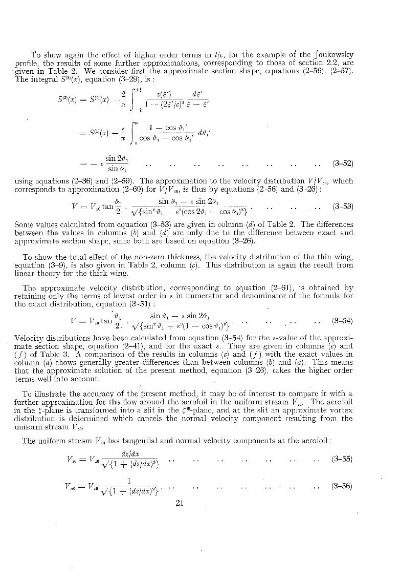
To show again the effect of higher order terms in t/c, for the exampie of the Joukowsky profile, the results of some further approximations, corresponding to those of section 2.2, are

g iven in Table 2. We consider first the approximate section shape, equations (2-56), (2-57). The integral S(al(x), equation (3-29), is :

S(~)(x ) = S l l ) (x ) _ 2 ~ [ +~ Z(~ I) d~'

2 - ~ 1 - (2~'/c) ~ ~ - ~'

_ i f ] 1 - - c o s # / dG' = S(1)(K) 2"~ COS ~'1 - - COS Wi t

sin 2G - - e sin G . . . . . . . . . . . . . . . . (3-52)

using equations (2-36) and (2-59). The approximation to the velocity distribution V/~o, which corresponds to approximation (2-60) for V/V,o, is thus by equations (2-56) and (3-26) :

V = V~Ù tan G sin G -- e sin 2~ 2 ~/{sin = #,, + d(cos 24i -- cos #1) ~} . . . . . . . (3-58)

Some values calculated from equation (3-53) are given in column (d) of Table 2. The differences between the values in columns (b) and (d) are only due to the difference between exact and approximate section shape, since both are based on equation (3-26).

To show the total effect of the non-zero thickness, the velocity distribution of the thin wing, equation (8-9), is also given in Table 2, column (c). This distr ibution is again the result from linear theory for the thick wing.

The approximate velocity distribution, corresponding to equation (2-61), is obtained by retaining only the terms of lowest order in s in numerator and denominator of the formula for the exact distribution, equation (3-51):

V = Vz0 tan G Sill ~1 -- e sin 2~ 2 " ~/{sin"G q- e= (1 - cos~9'1) 2} . . . . . . . . . (3--54)

Velocity distributions have been calculated from equation (3-54) for the e-value of the approxi- mate section shape, equation (2-41), and for the exact e. They are given in columns (e) and ( f ) of Table 3. A comparison of the results in columns (e) and ( f ) with the exact values in column (a) shows generally greater differences than between columns (b) and (a). This means that the approximate solution of the present method, equation (3-26), takes the higher order terms well into account.

To illustrate the accuracy of the present method, it may be of interest to compare it with a further approximation for t he flow around the aerofoil in the uniform stream K~.o. The aerofoil in the F-plane is transformed into a slit in the ~*-plane, and at the slit an approximate vortex distribution is determined which cancels the normal velocity component resulting from the uniform stream V~o.

The uniform stream V,0 has tangential and normal velocity components at the aerofoil :

d z / d x v,o = v,0 V { 1 + (&/dx) '~} . . . . . . . . . . . . . . (3 -55)

1

V,,o = V,o v '{1 + (&/dxp} . . . . . . . . . . . . . . . (3-s6)

21

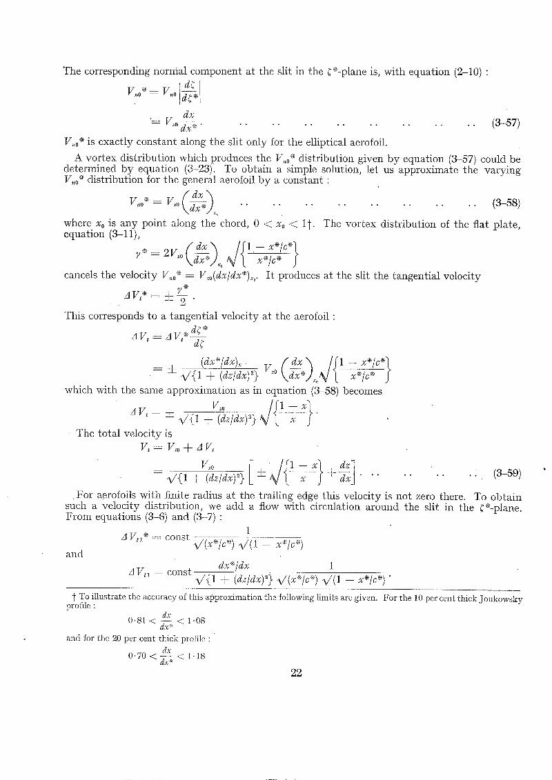
The corresponding normal component at the slit in the ¢*-plane is, with equation (2-10) •

V,o*= V,o ~

dx '= V~o dx,a, . . . . . . . . . . . . . . . . . (3-57)

V,0* is exactly constant along the slit only for the elliptical aerofoil.

A vortex distribution which produces the V,,0 "~: distribution given by equation (3-57) could be determined by equation (3-23). To obtain a simple solution, let us approximate the varying V~0* distribution for the general aerofoil by a constant •

V , , o * = V~o ~ .,, . . . . . . . . . . . . . . . . ( 3 . s s )

where x0 is any point along the chord, 0 < x0 < 1{. The vortex distribution of the fiat plate, equation (3-11),

dx

cancels the velocity V,,0* = V,o(dx/dx*).,.o. It produces at the slit the tangential velocity y *

AV,* = 4 -~ - .

This corresponds to a tangential velocity at the aerofoil •

z~ V, = z~ V, * ff¢''*- de

+

which with the same approximation as in equation (3-58) becomes

v, = 4- V ( 1 + (dz/dx) ~} The total velocity is

V t = V~0+AV~

= ~/{1 + (dz/dx) =} 4- + d-x . . . . . . . . . (3.59)

For aerofoils with finite radius at the trailing edge this velocity is not zero there. To obtain such a velocity distribution, we add a flow with circulation around the slit in the ¢*-plane. From equations (3-6) and (3-7) •

1 A Vt~* : const

and

A Vt~ = const dx*'/dx 1 v'{1 + (d~/d~)~} ,/(~"/~*) V'(1 -- ~*/~*)"

-~ To illustrate the accuracy of this approximat iol l the following limits are given. For the 10 per cent thick J o u k o w s k y profile :

dx 0.81 < ~ < 1.08

and for the 20 per cent thick profile :

d.v 0.70 < dx* < 1.18

22

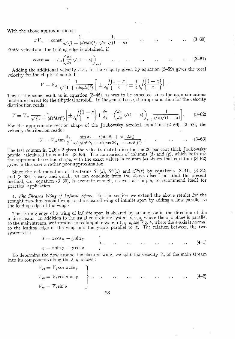
With the above approximations :

1 1 . . . . . . ( 3 . ~ 0 ) AYtl = const V,{1 + (dz/dx)~ } @x ~/(1 - - X ) ' "'

Finite velocity at the trailing edge is obtained, if

const = - V~0 dxx x/(1 -- x) . . . . . . . . . . . . . (3-61) X = I

Adding the additional velocity A Vt 1 to the velQcity given by equation (3-59) gives the t o t a l velocity for the elliptical aerofoil :

v = V~o ~/{1 + (dz/dx) ~} + - - ~ - - + ~ x "

This is the same result as in equation (3-45), as was to be expected since the approximations made are correct for the elliptical aerofoil. In the general case, the approximation for the velocity distribution reads :

y = v~0 ~ / { 1 + (dz/dx) 2} + x d ~ - - ~ ~ / ( 1 - - ~) .~:1 ~ / x ~ / ( 1 - - x) . ( 3 . 6 2 )

For the approximate section shape of the Joukowsky aerofoil, equations (2-56), (2-57), the velocity distribution reads:

V = V,0 tan Oj sin v~l -- e (sin 0.I + sin 2v~1) . . . . (3-63) 2"~/{sin~O~ + e~(cos2O~- cos~) ~} ' ..

The last column in Table 2 gives the velocity distribution for the 20 per cent thick Joukowsky profile, calculated by equation (3-63). The comparison of columns (d) and (g), which both use the approximate section shape, with the exact values in column (a) shows that equation (3-62) gives in this case a rather poor approximation.

Since the determination of the terms S(~l(x), S(~)(x) and S(3)(x) by equations (3.31), (3-32) and (3-33) is easy and quick, we can conclude from the above discussions that the present method, i.e., equation (3-30), is accurate enough, as well as simple, to recommend itself for practical application.

4. The Sheared Wing of Infinite Span.--In this section we extend the above results for the straight two-dimensional wing to the sheared wing of infinite span by adding a flow parallel to the leading edge of the wing.

The leading edge of a wing of infinite span is sheared by an angle ~0 in the direction of the main stream. In addition to the usua! co-ordinate system x, y, z, where the x, z-plane is parallel to the main stream, we introduce a rectangular system f, v, z, see Fig. 4, where the ~-axis is normal to the leading edge of the wing and tile v-axis parallel to it. The relation between the two systems is :

= xcos9 -- ysin~0 ; (4-1) • o • o , . . . • ° , • •

~7 = x sin ~0 + y cos ~0 3 To determine the flow around the sheared wing, we split the velocity Vo of the main stream

into its components along the ~, ~, z axes :

V~o = V0cos~cos~ "] I

V,~o = VocoS gs in~ F ,

J V~o = Vo sin

. . . . . . . . . . . . . . (4 -2)

23

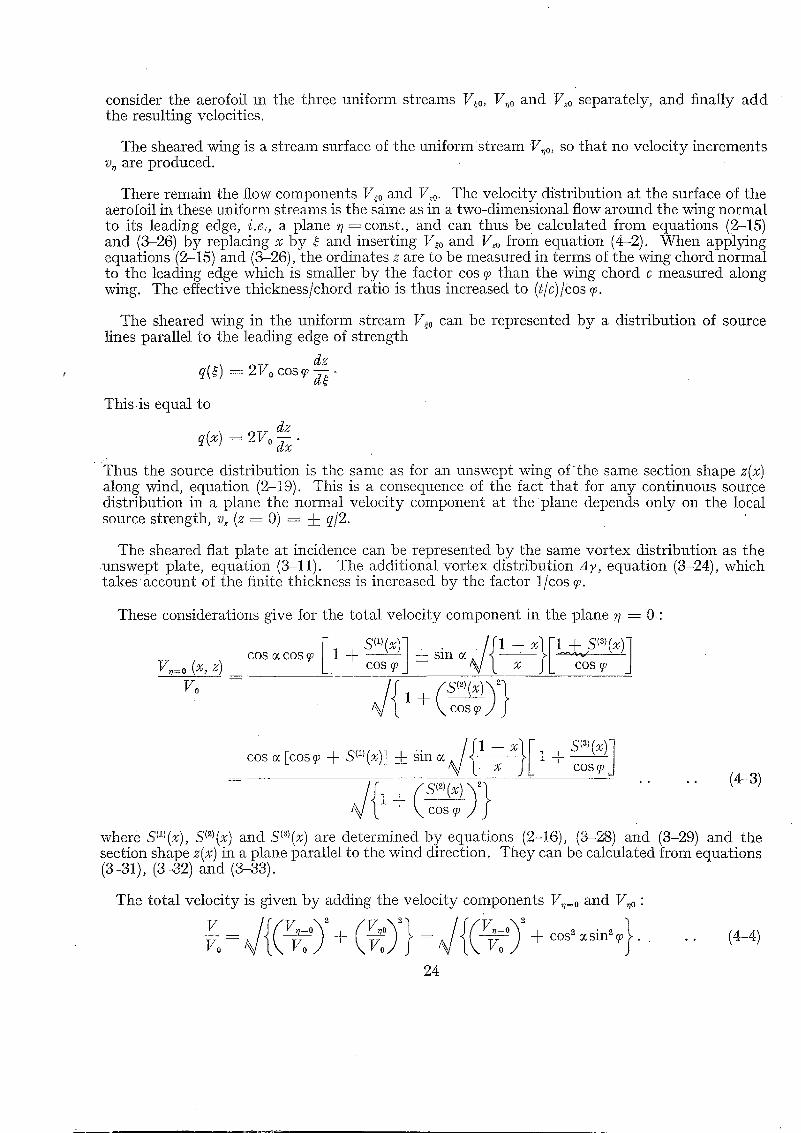
consider the aerofoil Ill the three uniform streams Va, V,o and V~o separately, and finally add the resulting velocities.

The sheared wing is a stream surface of the uniform stream V~o, so that no velocity increments v~ are produced.

There remain the flow components V,0 and V,o. The velocity distribution at the surface of the aeroIoil in these uniform streams is the same as in a two-dimensional flow around the wing normal to its leading edge, i.e,, a plane ~; = const., and can thus be calculated from equations (2-15) and (3-26) by replacing x by ~ and inserting V,o and V,0 from equation (4-2). When applying equations (2-15) and (3-26), the ordinates z are to be measured in terms of the wing chord normal to the leading edge which is smaller by the factor cos ~0 than the wing chord c measured along wing. The effective thickness/chord ratio is thus increased to (t/c)/cos %

The sheared wing in the uniform stream V,0 can be represented by a distribution of source lines parallel to the leading edge of strength

dz = 2V0 cos

This is equal to

dz = 2 V o

Thus the source distribution is the same as for an unswept wing of the same section shape z(x) along wind, equation (2-19). This is a consequence of the fact that for any continuous source distribution in a plane the normal velocity component at the plane depends only on the local source strength, v~ (z = 0) = -b q/2.

The sheared flat plate at incidence can be represented by the same vortex distribution as the unswept plate, equation (3-11). The additional vortex distribution AT, equation (3-24), wh ich takes account of the finite thickness is increased by the factor 1/cos ¢.

These considerations give for the total velocity component in the plane ~ = 0:

[ S(1)(x)] c~ / ~ 1 -- l <=0(x,z) cos cos 14 4- sin '%/t x JL cos j

cos o~ [cos¢-F S(1)(x)] :J:: Sin c~/<~--x}[ 1-I--- cos ~ j

(4 -3 )

where S(1)(x), S(~)(x) and S(8)(x) are determined by equations (2-16), (3-28) and (3-29) and the section shape z(x) in a plane parallel to the wind direction. They can be calculated from equations (3-31), (3-32) and (3-33).

The total velocity is given by adding the velocity components V~=0 and V~0 :

24

(4-4)

The velocity component in the spanwise direction %, which is needed for instance when calculating the shape of a strearriline, is given by •

] {4-5) v, _ sin 9 cos a cos • • v0 L v0 9 . . . . . . . . . . . . .

The pressure coefficient in incompressible flow is from equat ion (4-4) •

= 1 -- cos 2 c~sin 2 9 - -

and the chordwise loading "

cos ~. Ecos 9 + SI1)(x)] -t- sin ~ 1 + c~-~-sg.

1 + \ c o s g /

@ = 1 - - c o s 2c~sin s 9 -

(4-6)

( tic ~ (1 -- 2x) ~ 1 + \ c o s g / 1 -- (1 - - 2 x ) 2

CL = 2~(1-}- cost/C~9/ sin c~ cos9 . . . . . . . . . . . . . . . ('1-9)

The above relations show that, for wings of constant thickness/chord ratio tic along wind, the thickness corrections become larger with increasing angle of sweep. This implies tha t the greater the angle of sweep the more impor tan t it is to take the higher order terms in tic into account. For this reason, we have invest igated the accuracy of the present method, in sections 2.2 and 3.2, using the ra ther thick Joukowsky aerofoil with tic = 0-2 as an example.

W h e n deriving a formula for the pressure coefficient of a sheared wing by first de termining the linear order terms for the sheared wing and then applying a second-order correction, like equat ion (2-24), some doubt m a y arise as to whether the correction reads

1 1

~/{1 .+ (dz/dx) ~} or 1 -F \ c o s 9 / J

This quest ion is solved in favour of the second al ternat ive by the above derivat ion since this gives the exact answer for the aerofoil of elliptic cross-section.

25

(4-s)

This gives the lift coefficient •

[ A Cp = -- 4 cos c~ sin ct cos 9 1 -- x cos 9 / ' (4-7/

x 1 @ \ c o s g /

In tegra t ion of this distribution, equations (3-37) a n d (3-43), gives the lift coefficient.

As an example we quote the pressure distr ibution on a sheared wing of elliptic cross-section, (see equat ion ( 3 - 4 7 ) ) •

1 4- tic cos c~ cos 9 ± sin ~. cos 9J L x

Since no exact solutions exist for the three-dimensional flow. around swept wings, the accuracy of approximate solutions must be determined by comparison with experimental results. Part of the differences which occur are, however, due to the viscosity of the air which is neglected in the present calculations. To show the magnitude of such effects it is desirable to have a com- parison between calculated and measured pressure distributions on a sheared wing, for in this two-dimensional case we know that the present method gives sufficiently accurate results.

I t is difficult to s tudy a sheared wing of infinite aspect ratio in practice, since a sheared wing spanning a wind tunnel represents the conditions on a zig-zag wing, with the tunnel walls acting as reflection plates. The flow conditions existing near mid-semispan on a swept wing of finite aspect ratio are, however, similar to those on a sheared wing of infinite span, provided the aspect ratio is not smaller than about 4. Then the station considered is not affected by the distributions of the flow near the centre and the tips. The incidence, 0c, to be used in calculating the pressure distribution is the effective incidence, ~, which differs from the given geometrical incidence, %, by the induced angle of incidence, ~, produced by the trailing vortices :

= ~ = % - c~i . . . . . . . . . . . . . . . . . (4-10)

c~ has to be obtained from a calculation of the spanwise load distribution of the wing. In the following comparisons between theoretical and experimental results, the induced incidence has been calculated by the method of D. Kiichemann i° (195a). This method excludes wings of very small aspect ra t io; but it is only on wings unaffected by small aspect ratio effects that conditions exist which are similar to those on an infinite sheared wing, as discussed here.

Fig. 6 shows the chordwise load distribution measured near mid-semispan on a 45-deg swept- back wing of aspect ratio 5 (from Ref. 11), together with the calculated distribution. The calculation is made for inviscid flow. The comparison shows the effect of the boundary layer, present in the real flow, which is to reduce the circulation around the wing. The viscosity effect already exists for ~-+ 0, and increases with increasing incidence. The shape of the chordwise load distribution is also altered by the boundary layer, the more so the h~gher the incidence. Methods for calculating the pressure distributions on two-dimensional wings in viscous flow, when the growth of the boundary layer is known, have been described by J. H. Preston *~ (1949) D. Spence ~a (1952), G. G. Brebner and J. A. Bagley ~ (1952). A good approximation for small incidence can be obtained by ignoring the alteration of the shape of the chordwise load distri- bution and calculating the pressure distribution for a reduced effective incidence. The latter can be found from a calculated spanwise load distribution which uses the lift slope CL/o:~ of viscous flow for infinite aspect ratio. For the quoted example " CL/~ = 5.00 ~ inviscid flow • CL/% = 8.87 ; viscous flow, R = 1.7 × 106 : CL/% = 8.63.

A second example is given in Fig. 8, with experimental results from Ref. 15. In this case the wing is tapered. Ref. 16, which deals with the calculations of the pressure distribution on swept wings at zero lift, contains a discussion of how the three-dimensional flow around a tapered wing can be approximated by a series of ' local two-dimensional flows '. In this approximation the pressure distribution at a station free from centre and tip interference is calculated from the formulae for the sheared wing of constant chord by taking for each point along the chord its

geometri,~ sweep ~(x), i.e., the sweep of lines joining points of constant percentage chord

In Fig. 8, two calculated curves are given for the load distribution on the thick wing. In one calculation the local angle of sweep ~o(x) was used. The other calculation was made with a constant ~0 along the chord, i.e., the angle of sweep at mid chord, ~o~/=. The two different chordwise load distributions give different values of CL/o:~ ( a . 8 7 for ~ = ~(x), 4 . 1 2 for ~ = %/~) and con- sequently different values of CL/% (2.79 for ~v = ~o (x), 2.91 for q0 = %/2). Since the experimental results are also affected by the viscosity of the air, it is not possible to conclude from this test t

t i t is difficult to isolate the taper effect from experirnentM results on more highly tapered wings since these are wings of small aspect ratio and it is known that, with straight constant-chord wings of small aspect ratio, the chordwise load distribution differs from the two-dimensional distribution.

26

whether to use the local ~(x) or the constant ~oo/~. To show that the effect of this uncer ta inty is not large compared with the effect of the finite thickness, tile load distributions of thin wings are also plotted in Figs. 6 and 8.

5. The Centre-section of a Swept W i n g . - - T o solve the problem of calculating the pressure distribution at any station of a swept wing, a further basic problem is the determination of the pressure distribution at the centre section of a swept wing of infinite aspect ratio.

The solution for zero lift has been dealt with in detail in Ref. 16. The problem was solved by replacing the wing by a distribution of kinked source lines. The strength of the source distri- bution is, in linear theory, again given by equation (2-19), since the vz-velocity on the chord-line produced by a continuous distribution of kinked source lines is still equal to q/2. This implies tha t in linear theory the problem is a ' quasi two-dimensional ' one, since for wings of constant section shape the source strength does not vary on lines parallel to the leading edge.

I t was shown that the source distribution produces a velocity component, v,., at the chord-line of the centre-section which differs from that on the sheared wing, cos 9. S l~)(x), by an additive term dependent on the local source strength"

v,(x, z = O) q(x)

Vo - c o s % S ( ' ( x ) - f ( v ) c o s ~ 2V0

dz = cos % s ( ' ( x ) - f ( ~ ) c o s ~

= cos ~ iS l~ ) ( x ) - f ( ~ ) cos ~ . S ( ' l ( x ) . . . . . . . . . . ( 5 - t )

with

f(~) = - l l n 1 + sin9 .. . . . . . . . . . . . . (5-2) 1 -- sin ~0

The spanwise velocity component vy is zero by reasons of symmetry.

To obtain the velocity distribution on the surface the correction factor of the straight wing, equation (2-24), is again applied:

V(x, z) _ 1 q- cosg.S°/(x) -- f(~0) cos ~0.S(2/ (x) . . . . (5-3) v0 - V { 1 + (s~2~(x)) ~} . . . . . .

and C, = 1 - {1 + cos~ .S ( ' ( x ) - f (~) cos~.S(~l(x)} 2

1 q-(S(21(x)) 2 . . . . . . (5-4)

This gives only an approximate result, but the comparison with experimental results, given in Ref. 16, shows sufficient agreement for practical purposes. There are no exact solutions available to determine the accuracy of the method, nor are there known any better approxi- mations which might be obtained by calculating the velocity components at the surface which are produced by a source distribution of constant strength along lines parallel to the leading edge. The exact solution demands source distributions 0f varying strength along these lines.

The infinite source strength at the leading edge, which results from the assumptions of linear theory, leads to a pressure coefficient at the leading edge different from 1. An approximate formula, giving the correct stagnation pressure at x = 0, is :

) "L I + cos~.S(')(~)-f(~) cos~ </{I + (s(',(,~))'}]

c , = 1 - . . . . ( 5 - 5 ) 1 + (S <2'(x))"

27

The difference between the formulae (5-4) and (5-5) is important only within the first few per cent of the chord. This is illustrated in Fig. 5, where the pressure distributions calculated from the two equations for 12 per cent thick wings with 45-deg sweepback are plotted, together with experimental results.

Measurements of the pressure coefficient on swept wings at incidence have shown that the shape of the chordwise load distribution at the centre-section differs from that of the distribution further outboard. I t has been explained in Refs. 10 and 17 that this is due to the fact that the v,-velocity produced by a distribution 7 (x) of kinked vortex lines of infinite length and constant strength along the span is no longer given by equation (3-12) but by the relation :

v,(• , , ) = - 2-; r ( * ' ) . _ . , + . . . . . . . . . (s-G)

The term a can be approximated with sufficient accuracy for all points along the centre-line by the constant

a = = tan ~0 . . . . . . . . . . . . . . . . . (5-7)

The term --~7~.y(x) corresponds to the term --f(~0)cos~0 in equation (5-1.) for the

v cvelocity induced by a distribution of kinked source lines of infinite length'.

A solution of equation (5-6) which gives the constant v,-velocity

v~ = V~o = Vo sin along the chord, is the vortex distribution

with

Q1 -- x) ~ y(x) = 2go sin. ~cos~ x (s-s)

As stated in Ref. 10, the vortex distribution of equation (5-8) can also be used for the centre- section of ordinary swept wings with non-uniform loading for which ~(x) varies along the span. The vortex distribution of equation (5-8) must now replace the distribution of equation (3-11) for the unswept flat plate.

Our aim is to find a vortex distribution corresponding to equation (3-25) which also takes into account the thickness of the aerofoil. I t is impossible to determine analytically a correction to the vortex distribution of equation (5-8) similar to the A y (x) of equation (3-24) for the straight wing. Equations (5-6) and (5-7) have not yet been verified analytically for the thin wing, but only numerically for wings of finite thickness, by calculating the downwash which a vortex distribution at z = 0 produces at the surface of thick aerofoils. These calculations lead to a-values in equation (5-6) which vary slightly along the chord and with the thickness/chord ratio, and the shape of the aerofoil. These variations have been ignored in equations (5-7) and (5-8).

Tentatively, therefore, we Use the factor (1 + S(~/(x)) of the two-dimensional wing to multiply the ~(x) of equation (5-8):

(1 -- x)'~(~) (1 -t- S(a)(x)) . . . . (5-10) 7(x) = 2V0 sin ~cos~o x " . . . .

in analogy to the procedure for the infinite sheared wing.

28

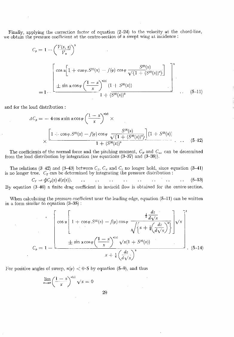
Finally, applying the correction factor of equation (2-24) to the velocity at the chord-line, we obtain the pressure coefficient at the centre-section of a swept wing at incidence •

c , = l - \ Vo /

cos el1 + cos~0.S(')(x) -- f(~) cos9 S(~)(x) ] ~/{1 + (sc~>(~)?}/ | / 1 -- x \ <~) L 4 - s i n c ~ c ° s ~ Q x ) ( l+S'~)(x))

= 1 - 1 -]- (S(~)(x)) 2 .. (5-11)

and for the load distribution •

A @ 4 cos c~ c~ cos ~o k ! X

1 + c o s ~ . S C ' ) ( x ) - f ( ~ ) cos~ V { 1 + (s(~(~))~}J

x 1 + (s~(x)) ~ . . (5-12)

The coefficients of the normal force and the pitching moment, C~ and C .... can be determined from the load distribution by integration (see equations (3-37) and (3-38)).

The relations (3=42) and (3-43) between Cr, CN and CL no longer hold, since equation (3-41) is no longer true. Cr can be determined by integrating the pressure distribution •

c~ = CG(~)d(~(x)) . . . . . . . . . . . . . . . . . (5-13) By equation (3-40) a finite drag coefficient in inviscid flow is obtained for the centre-section.

When calculating the pressure coefficient near the leading edge, equation (5-11) can be written in a form similar to equation (3-35) •

COS 0¢ [

1 dz

1 + cos ~.S/l'(x)-/(~) cos~--.dfx + !('-dz-'~'\dVx./J

(1-x)"'~'V.x( 1 + S,~,(x)) ± sin ~ cos 9 x

]+xl c , = 1 - (5-14)

For positive angles of sweep, n(~0) < 0.5 by equation (5-9), and thus

lira (.1 -- x)"/~) %/x = 0 x---->-0 X .

29

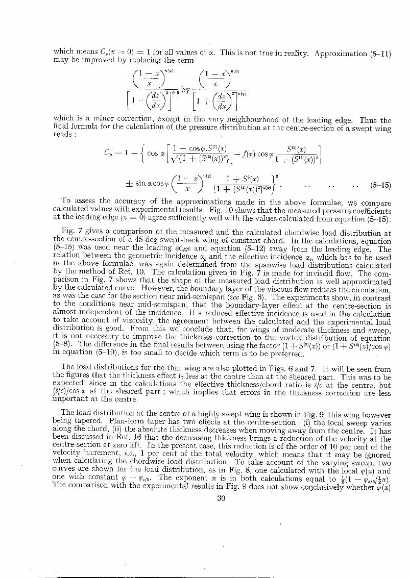
which means C / x = O) = 1 for all values of a. This is not true in reality. may be improved by replacing the term

<1 --x x) "('~) <1 --x x) ~(~1

I l +<dxx) J/dz\27°'5 by [l + ~,dx/]ddz~]'~(~)

Approximation (5-11)

which is a minor correction, except in the very neighbourhood of the leading edge. Thus the final formula for the calculation of the pressure distribution at the centre-section of a swept wing reads :

c,= - cos + (s(,,(x)),}.- y(v) cosy I +

[I + (s(')(x))']-(,)J " ""

To assess the accuracy of the approximations made in the above formulae, we compare calculated values with experimental results. Fig. 10 shows that the measured pressure coefficients at the leading edge (x ---- 0) agree sufficiently well with the values calculated from equation (5-15).

Fig. 7 gives a comparison of the measured and the calculated chordwise load distribution at the centre-section of a 45-deg swept-back wing of constant chord. In the calculations, equation (5-15) was used near the leading edge and equation (5-12) away from the leading edge. The relation between the geometric incidence % and the effective incidence ~, which has to be used in the above formula% was again determined from the spanwise load distributions calculated by the method of Ref. 10. The calculation given in Fig. 7 is made for inviscid flow. The com- parison in Fig. 7 shows that the shape of the measured load distribution is well approximated by the calculated curve. However, the boundary layer of the viscous flow reduces the circulation, as was the case for the section near mid-semispan (see Fig. 6). The experiments show, in contrast to the conditions near mid-semispan, that the boundary-layer effect at the centre-section is almost independent of the incidence. If a reduced effective incidence is used in the calculation to take account of viscosity, the agreement between the calculated and the experimental load distribution is good. From this we conclude that, for wings of moderate thickness and sweep, it is not necessary to improve the thickness correction to the vortex distribution of equation !5-8). The difference in the final results between using the factor (1 + S(3)(x)) or (1 + S(3)lx)/cos cp) m equation (5-10), is too small to decide which term is to be preferred.

The load distributions for the thin wing are also plotted in Figs. 6 and 7. I t will be seen from the figures that the thickness effect is less at the centre than at the sheared part. This was to be expected; since in the calculations the effective thickness/chord ratio is tic at the centre, but (@)/cos ~ at the sheared par t ] which implies that errors in the thickness correction are less important at the centre.

The load distribution at the centre of a highly swept wing is shown in Fig. 9, this wing however being tapered. Plan-form taper has two effects at the centre-section : (i) the local sweep varies along the chord, (if) the absolute thickness decreases when moving away from the centre. I t has been discussed in Ref. 16 that the decreasing thickness brings a reduction of the velocity at the centre-section at zero lift. In the present case, this reduction is of the order of 10 per cent of the velocity increment, <e., 1 per cent of the total velocity, which means that it may be ignored when calculating the chordwise load distribution. To take account of the varying sweep, two curves are shown for the load distribution, as in Fig. 8, one calculated with the local ~(x) and one with constant ~ ---- %/~. The exponent ~¢ is in both calculations equal to ½(1 -- %/2/~a). The comparison with the experimental results in Fig. 9 does not show conclusively whether ~ (x)

30

or %n gives the bet ter agreement. This implies tha t we cannot decide from this test whether to take the factor (1 + S(~l(x)) or (1 + S(31(x)/cosg~) in equations (5-10) and (5-11). I t must be pointed out, however, tha t the differences between the various methods themselves, and between calculation and experiment, are small compared with the differences between the distr ibutions at the centre and near mid-semispan. We can, therefore, conclude tha t the present me thod provides sufficiently accurate results for most practical purposes.

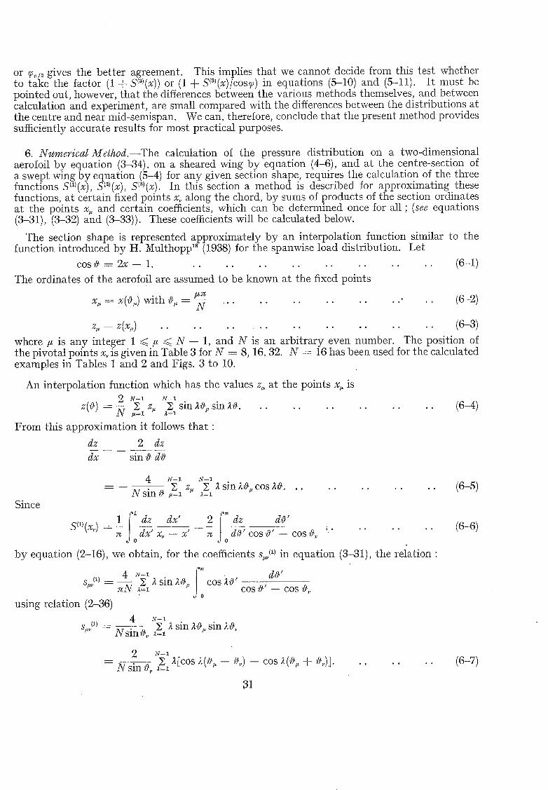
6. N u m e r i c a l Me thod . The calculation of the pressure dis t r ibut ion on a two-dimensional aerofoil by equat ion (3-34), on a sheared wing by equat ion (4-6), and at the centre-section of a swept wing by equat ion (5-4) for any given section shape, requires the calculation of the three functions Sl~(x), S(2)(x), S(3)(x). In this section a me thod is described for approximat ing these functions, at certain fixed points x,, along the chord, by sums of products of the section ordinates at the points x~ and certain coefficients, which can be de termined once for a l l ; (see equat ions (3-31), (3=32) and (3-33)). These coefficients will be calculated below.

The section shape is represented approximate ly by an interpolat ion function similar to the funct ion int roduced by H. Multhopp TM (1938) for the spanwise load distribution. Let

cos v~ = 2x -- 1 . . . . . . . . . . . . . . . . . (6-1)

The ordinates of the aerofoil are assumed to be known at the fixed points

x. = x(v~.) with v~,, =/~--~ . . . . . ' . . (6-2) N ,o . • • o , .

z . = . . . . . . . . . . . . . . . . . . .

where /z is any integer 1 ~</z ~< N - 1, and N is an arbi t rary even number. The position of the pivotal points x, is given in Table 3 for N = 8, 16, 32. N = 16 has been used for the calculated examples in Tables 1 and 2 and Figs. 3 to 10.

An interpolat ion function which has the values z,, at the points x, is 2 g - - i N--I

z ( ~ ) - - N ~ z ~= ~=~E s i n 2 ~ s i n ~ . . . . . . .

From this approximat ion it follows tha t •

dz 2 dz

( 6 - 4 )

dx sin v~ d~

Since

4 N--I N--I

= - - N s i n v ~ ~1= z~ ~=~X ;t sin 10~ cos 2 ~ .

z~ dx ' x~ - - x ' zc de ' cos v a' -- cos ~ '

by equat ion (2-16), we obtain, for the coefficients s~v/1) in equat ion (3-31), the relation •

-- X 2 sin iv~ cos ~z~' v~' -- S"~(~) ~ N ~.-1 COS COS va.,,

using relation (2-36) 4 N - - 1

- - E 2 sin 20~ sin 2v~, s~// N sin v~, a=~

(c-s)

2 N - - 1

- N s i n e . [cos - - c o s +

3 1

(6-7)

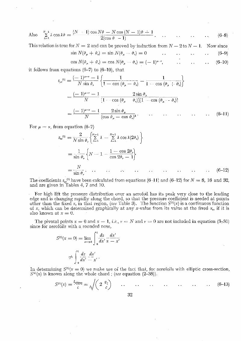
N--1 ( X - 1 ) C O S N O - - ' N C O S ( N - 1 ) 0 --~ l Also X ~ c o s ~ =

~ = ~ 2 ( c o s ,o~ - 1 ) . . . . . .

This r e l a t ion is t r u e for N = 2 a n d can be p r o v e d b y i n d u c t i o n f r o m N - - 2 to N - - 1.

sin N ( ~ . + G) = sin N ( 4 . - - G) = 0 . . . . . . .

cos N(G + o~) = cos N(G - o,) = ( - 1) .-~, . . . .

i t fol lows f r o m e q u a t i o n s (6-7) to (6-10), t h a t

{ ' i} s~(~) = ( - - 1)"-" - - 1 1 cos - - cos q- G N sin 0~ - - (0, - - G) 1 - - (0,

. . (~-8)

N o w since

. . (6-9)

. . (6-1o)

(-- 1) "-~ - - 1 2 sin 0 ,

N E1 - - cos (G - - G)][1 - - cos (G + G)]

( - - 1) "-~ - - 1 2 sin # , N

F o r / ~ = v, f r o m e q u a t i o n (6-7)

s'(~) - - N sin G ( ~=1

(COS tg~, - - COS Or) 2 "

1 - - 2: ;t cos 1 (2G) 1=1

(6-11)

1 I N - 1 1 - c o s 2 4 Q - - s i n g L co~-2~T-- i J

i v . . . . . . . . . ( ~ - 1 2 ) - - . . , , . .- , . . sin G

T h e Coefficients s,~ cll h a v e b e e n c a l c u l a t e d f r o m e q u a t i o n s (6-11) a n d (6-12) for N --= 8, 16 a n d 32, a n d are g iven in Tab le s 4, 7 a n d 10.

F o r h i g h lift t h e p res su re d i s t r i b u t i o n ove r an aerofoi l has i ts p e a k v e r y close to t he l e a d i n g edge a n d is c h a n g i n g r a p i d l y a long t he chord , so t h a t t h e p re s su re coeff icient is n e e d e d a t p o i n t s o t h e r t h a n t h e f ixed x~ in t h a t region, (see T a b l e 3). T h e f u n c t i o n SCll(x) is a c o n t i n u o u s f u n c t i o n of x, w h i c h can be d e t e r m i n e d g r a p h i c a l l y a t a n y x -va lue f r o m its v a l u e a t t he f ixed x , if i t is also k n o w n a t x = 0.

T h e p i v o t a l p o i n t s x = 0 a n d x = 1, i . k , v = N a n d v = 0 are n o t i n c l u d e d in e q u a t i o n (37-31) s ince for aerofoi ls w i t h a r o u n d e d nose,

i1 dx' Sm(x = 0) = ,-+olim Jo dxd-~z' x - - x '

i 1o dz dx' =/: dx ' - - x ' "

I n d e t e r m i n i n g SIll(x ---- 0) we m a k e use of t he fac t t h a t , for aerofoi ls w i t h e l l ip t ic cross-sect ion, Sill(x) is k n o w n a long t he whole c h o r d ; (see e q u a t i o n (2-35)).

32

where e is the nose radius. We subtract from the aerofoil ordinates those of the elliptic aerofoil wi th the same nose radius •

_ _ . . . . . . . . . . . (6-14)

W i t h convent ional aerofoil sections we can assume tha t A z has no term which varies l inear ly wi th x. T h e n '

dAz dx ' dAz dx' lim -- x' -- x' ~--~o d x ' % d%' - -

o

N--1 ~ SpN (i} ZJ Z/, '

p= l

with S,uN{1 ) = (-- 1) ~ -- 1 2 sin v~.

N i i + cos ~.)~ from equat ion (6-11). For the ellipse

z . , = ~ c sin ~.

6 - 1 s )

~-~ t ~ (-- 1 ) ' - - 1 sin~ ~, ~ S~N (I) Z~ -- /* = I - C ,u=l N (1 + COS %~,u) 2

_ t_, [_ ( N - 1 ) ] . c

2 -~-- ~ S/~N (1) Z/,- ~ S#N(1)Z~/2 • p=l j*=l

Since

S('(x = 0) =

we obta in finally,

S(1)(x = O) = N 2 + ~. s~N~l) z# . . . . . . . . . . . .=1

The term S(2)(x), which is equal to the slope of the profile surface dz/dx, can of course, be determined graphical ly from a plot t ing of z against x, but it can also be determined numerical ly at the points x . F rom equat ion (6-5) we obtain a relation for the coefficients s~J ~) in equat ion (3-32) •

4 N-I s~J2) -- N sin ~. ~ t ~ sin ;t~. cos ~

Now

2 ( ' E l ;~[sin t(~9. + a~) -}- sin ;~(4~- 4,)]~ . . . . . (6-17) N sin #,~ ( ~ = i )

N-1 (N - - 1) s i n N o - - N s in ( N - - 1)~ (6 -1S) X ~ sin ~9, = 2(cos ~9 -- 1) 2=1

33

This relation is true for N = 2 and can be proved by induct ion from N -- 2 to N -- 1. equat ion (6-9) it follows from equations (6-17) and (6-18) tha t •

sin(v~ + G) sin(v~, - - G) ] sg) -- (-- 1)~-~ 1 cos + 1 -- cos d n e.. - (% e..) + - <)

( i 1)"-" { '0 , - I- G va, -- G} -- sin 0r cot 2 + cot 2

= -- 2 (-- 1)"- 's inO, sin G [cos ~ -- cos G] "

For ~ = ~, from equat ion (6-17) •

2 N--1

s"'?) = -- N sin v~,- ~=~X ,~ sin 2;~G

Using

(6-19)

1 sin 2G sin v~,, 1 ~- cos 2va,

cot 0r sin ~ "" "" (6-20)

N--~ sin e ~. - ( - 1 ) . = 1 . o

~=* 1 + cos v*,,

so tha t for the elliptic aerofoil, z = ½(t/c) sin a, (dz/d~/x).,=o = t/c, which agrees with the exact value, F?r the 20 per cent thick Joukowsky profile equat ion (6-23 gives dz/d~/x ---- 0" 2991 whilst

34

Now

N-- 1 sin ,9 = - - 2 E ( - - 1) '< z,., . . . . . . . (6--23)

,,-1 1 + cos v~ . . . .

The coefficients G] ~/ calculated from equat ions (6-19) and (6-20) for N = 8, 16 and 32, are given in Tables 5, 8 and 11.

In calculating the pressure distr ibution at high incidence by equat ion (3-35) the derivat ive of z with respect to ~/x, dz/dv/x, is needed. This term can be de termined graphically from a plot t ing of z against a /x or by plot t ing

taking into account the relation

The values of dz/d,v'x determined by equat ion (6-21), or directly from plot t ing z(v'x), need not fully agree since equat ion (6-5) is only an approximation. The magni tude of the difference can be seen by comparing the exact nose radius with the radius of the approximate section shape, equat ion (6-4). From equat ion (6-5) it follows tha t

%

d z

the exact value from equat ion (2-53), (2-54) is 0.2992. For the 10 per cent thick RAE 101 section the nose radius from equat ion (6-23) is o/c ---- 0.00760, whilst the figure given in Ref. 9 is e/c---= 0.00763. These figures show tha t for aerofoil sections which have a shape similar to an ellipse for the first few per cent of the chord, the interpolat ion formula (6-4) is adequate.

If there is an appreciable difference between the two values for the nose radius, one might improve the interpolat ion formula (6-4) by adding the te rm (c]N) sin N#~ :

2 N - 1 N - 1 c , • z(#) = ~ ,~: z~ ~:lX sin Z0, sin Z0 + ~ sin NO . . . . . . . . . (6-24)

This interpolat ion function gives the required values at x~, :

Thus dz 2 N-1 N-1 dO -- N ~ : z, ~=IE Z sin Z#. cos ~9, + c, cos N# . . . . . . . . . (6-25)

The constant c, can be chosen so tha t

( d z ) ~-~ sin#,, ~=,= Z (-- :t)" z~+c, ~=~ 1 + cos #~,

. . . . . . . . . . . . . . . • •

The improved interpolat ion function (6-24) gives the same values for S(~)(x,,) as equat ion (6-4), since the addi t ional te rm to S(~l(x) is by equations (6-6) and (6-25)

2c, ['= d , ' s i n N # zJ S(1)(tg) = - - 3o cos N# ' = 2c, - - . . . . . . . . (6-27) cos #' -- cos 0 sin ,9

which is zero for # = #,. At the leading edge, # = ~, ASI~I(x) = - - 2Nc,, i.e., N t imes the dif- ference between the values of 1/(2e/c) for the given section and the interpolat ion function, which means S(~l(x = 0) is given by equat ion (6-16).

Th~ a m e n d m e n t of the interpolat ion function z(#), given by equat ion (6-24), is a special case of the a m e n d m e n t suggested by J. WeissingeP ~ (1952) for calculating the spanwise load distri- but ion using the calculation me thod by H. Multhopp ~8.

The interpolat ion function equat ion (6-4) gives the correct ordinates at fixed points x,. It may be desirable to calculate the function S(~l(x) from an interpolat ion function z(v~) which has the correct value z~ at one further arbi t rary point x~. Let an asterisk denote the values of z and S(1/. ob ta ined from equat ion (6-4). The new interpolat ion function is

= + - z * ( o o ) sin N0~ sin NO . . . . . . . . . . . (6-28)

By equat ion (6-6),

S(1)(O ) = S(1)@(19,) -~- ,~(tg'a) - - Z@(tg'a) 2 N s i n N # . . . . . (6-29) sin Nv% sin # " " "

-~An ~dditive term which does not alter the section shape of equation (6-~) at the trailing edge is (G/N) sin 27#.-}(1 -- cos #). To obtain the required nose radius the constant c, is to be determined by equation (6-26). The additive term alters the value of S(1)(x)~ slightly. I t follows from equation (6-6) that the additional term to

• S(~)(x~) is: (-1),

AS(1)(x~) = - - N c,

This correction can usually be neglected since c, is generally small.

5

Therefore, sin N~, = 0 by equation (6-2),

S(1)(t9~,,) = S ( 1 ) * ( l ~ v )

i .e. , the values of S ( l l ( x ) a t the points x,. are not altered by using a fur ther point for determining the interpolat ion function. This is not so for points 0 =/= tg,. In particular,

s~l~(~o) = s~l~*(~) + [z(o,~) - z*(<)] s ~ T h i s relation can be wri t ten in the form :

N--1 S(1)(~ , ) = s~Cl)z~ + 2 s,~o< z,, . . . . . . . . . . . . . . ( 6 - 3 0 )

i*=1

where

2N Sag(l) ---- sin ~ ,~- - . . . . . . . . . . . . . . . . . . (6-31)

- - 4 N - - I

s"]l) -- N sin 0s ~1 (N -- 2) sin ha, sin ~ , . . . . . . . . . . (6-32)

by equations (3-31), (6-4) and (6-7).

t ha t

I t follows from equation (6-8) a n d t h e relation

N-~ cos (N -- 1)# -- cos Nv~ + cos v~ -- 1 E cos Z# . . . . . . . . . (6-33) a=~ 2(1 -- cos ~)

2 sin v~, [cos N~9, cos N~9, 1] s"]~) = NEcos ~, -- cos v%]

where

4 sin #. N [ c o s a, , - c o s a~ l " A , o . . . . . . . . . . . . ( 6 - 3 4 )

A,, , = sin2 N2~ for ff even

cos 2 ~ f o r ff o d d .

If in par t icular #4 = {(2~ q- 1)/2N}a, i.e., at a pivotal point of the sys tem with 2 N p o i n t s taken along the chord, then A,,~ = } for all ¢ and a, and the coefficients s,,~ I1) by equation (6-34) agree wi th those by equation (6-11) calculated for 2N.

We have s ta ted in section 2.2 tha t the interpolat ion function, equat ion {6-4), replaces the given section by one wi th a finite radius Or at the trai l ing edge. We will now determine this radius. We have

dz

N-~ sin 0,. = - 2 ~ ( - 1)~ ~ . . . . . . . . . . . ( 6 - 3 5 )

.=1 1 --= COS ~

For the 10 per cent th ick R A E 101 section, equation (6-35) gives or/c = 0. 000009, which means there is no impor tan t difference between the given section and the approximation,

a 6

Final ly , we have to d e t e r m i n e the coefficients s,,/~i a n d sN~ (3) i n e q u a t i o n (3-33) for the f u n c t i o n Sl~l(x,)'~. F r o m equa t ions (2-16) a n d (3-29)"

2±~ 1 z(x') dx' S(~)(x) = Sa)(x)

1 - - (1 - - 2x')~x - x' L = S(~)(x) + 2 L z ( # ' ) ( ' ' ~ dS' . . . . . . ( 6 - 3 6 )

s i n 8 ' c o s 8 ' - - c o s 8 " ' " l ) e

TO e v a l u a t e the in tegra l we a p p r o x i m a t e to the va lue of z(O)/sin 8 b y an in t e rpo la t ion funct ion . The func t ion

F 2 N - i N-1 ] --sin sin sin 48 ] sin O sin 2 #~ ~=1

~/(~) I sinN# I -- cos#

-- 2cc N sin # 2 " '

has the r equ i r ed va lues at # = 8~, since sin (NG) = 0, l ead ing edge, 8 : ~ •

. . . . . . . . (6-37)

I t also h a s the correc t va lue a t the

s ince

s i n N # 1 - - c o s 0 ) = _ N"

At the t ra i l ing edge, O = 0, equa t ion (6-37) gives z(8)/sin O = 0,' wh ich is correc t for aerofoils w i t h a sharp t ra i l ing edge.

B y equa t ions (6-36) a n d (6-37), we obta in , for the coefficients s.] ~/ in equa t ion (3-33), the

sin 48' sin 8' dS'

COS #t __ COS 0 . "

j c o s (4 - - 1 ) O ' - - c o s (2 q- 1 ) 8 '

COS 8 ' - - COS O,, 0

do'

re la t ion •

4 1 N--1 ;~ I; sin ;~O~, G)3) = s~']l) q- a N sin" 8~ ~=~ J°

B y m e a n s of equa t ion (2-36) '

f l sin 8' dO' _ sin 4,0' 8 ' - - - - ~ COS COS 8~

Thus •

sin (4 -- 1)G = sin (4 + 1)8. 2 sin v%

= - - ~ cos 4G . . . . . . . . . . . . . . . . . (6-38)

4 I N--I - - - - = I; sin 28~, cos 48,,

2 I N--I = s~5~ Nsin~0~ ~1 [sin;~(,L + ,L) + sin 4(G -- 'L)] . . (6-39)

]-For aerofoils with finite radius of curvature 0z at the trailing edge, a further t e rm so,,(a)V'(~H2c ) has to be added in equation (3-33). Excep t for the elliptfc aerofoil, such aerofoils are of little practical interest:

37

N-, s in (N - - 1)4 - - sin NO 4- sin # N o w Z s in Z# =

~=1 2(1 - - cos O) . . . . . . . . . .

w h i c h m a y be p r o v e d b y i nduc t i on . Us ing e q u a t i o n s (6-9), (6-10) a n d (6-40) we o b t a i n

S/~ (8) ~ S[~ (1) - -

1 - - ( - - 1) ' -~{ s i n ( G 4 - G ) s i n ( # , , - 5 ) "~ Nsi~o,~ 1 - cos (o,. + m) + 1 2 ; G ( C _ o.) j

COS O'~ -- COS O~

a n d hence

2 1 - - ( - - 1 ) ~ -~ s~]3) = s~(~) + _~ sin # .

F o r ¢ = v, we o b t a i n f r o m e q u a t i o n (6-39)

2 1 N--1 = t; s in A(2G) sJa) sJ') N sin ~ O~ z=~

(6-40)

(6-41)

2 1 sin [(N -- 1)2G] 4- s in 2O. S~, (1)

N sin 2 G 2(1 - - cos 2G)

S~ (1) . . . . . . . . . . . . . . .

B y e q u a t i o n s (6-36) a n d (6-37), t he coeff icient s,w (~) in e q u a t i o n (3-33) is

1 s i n N # ' 1 - - c o s 0 ' s g / = = N j o s~n~ ' cos 0 ' - - cos G d0 '

(6-42)

N o w

2 ~ N Jo sin O' cos O' - - cos G

= I=sin ~O' d# '

Y~ j0 ~n V co~ o ' - cos o

(6-43)

1 - - COS ;~0, = ~ for .t even

sin ~ O.

cos O~ -- cos AO~ s i l l ~ #,,

as can be p r o v e d b y t he r e l a t ion

sin (2 - - 1)G sin v%

w h i c h fol lows f r o m

sin ZO sin O

sin (4 - - 2)# sin #

There fo re , u s ing t he e q u a t i o n s

J1 = 0

for ,~ o d d . . . .

+ 2cos (~ - 1)#.

(6-44)

2 ~ 2P'/:

38

N being an even number, equat ions (6-43) and (6-44) give

~ 9 ~ _ ( - ~)~- ~ 1 . . . . . . . . (645) • N " 1 + cosG "" ""

The coefficients s#,? I have been calculated from equations (6-41), (6-42) and (6-45) for N = 8, 16 and 32, and are given in Tables 6, 9 and 12.

Using these coefficients S(a/(x) can be calculated for the points x,. Since sial(x) is a continuous function, its values at points other than x. can be determined graphical ly if S(')(x = 0) is known.

In determining Sla/(x = 0) we apply the same procedure as in determining S<(x = 0). We subt rac t from the given section ordinates those of an elliptic aerofoil, equat ion (6-14), and make use of the fact t ha t for elliptic aerofoils

t ~ m ~ o ` / ( 2 @" ~ (6-46, S~3~(x) _ _ - - ~ , . , , o , . o o o o , ° o

C N k C /

(see equat ion (3-46)). For the Az of equat ion (6-14) we have

N - - 1 A S I~l(x = O) = E s,,~(~lA z,,

/*=1

with

S#N (3) ~ S I g N (1) @

2 l - ( - 1), 1 N sin 4~ 1 - / cos v~

2 [1 - ( - 1)q cos,L -- N sin 0# (1 + cos v~)

by equations (6-15) and (6-41). For the ellipse, z,. = ½

N - - 1 t e N - - 1 1 - - ( - - 1)" c o s G

° f i n "'el* - - ,=l c ~,=1 N 1 q- cos v~

• ° o

t_~ sin ,~,, C

. . (6-47)

Then, from

S t ~ N ( 3 ) Z t , SZ a,r(3)~'e/~ S(3~(x = O) = 2 + .=1 - . = 1

we obtain finally

N - - 1

E S, NI3)Z,, . . . . . . . . . . . (6-48) l* = 1

7. Calculated E x a m p l e . - - T o i l lustrate the calculation procedure a worked example will be given. We calculate by equat ion (4-6) the pressure dis t r ibut ion on a sheared wing, swept b y an angle 9 = 45 deg, at an incidence ~. The aerofoil section parallel to the main s t ream is a twelve per cent th ick R A E 101 section (see Ref. 9).

' 39

The layout of the calculation is given in Table 13, for N = 16, i.e., we fix the section shape by its ordinates at 16 points along the chord. This n u m b e r of points does not involve a great amoun t of computa t iona l work and gives results of sufficient accuracy for almost all pract ical cases.

F rom the given section data , wi th the co-ordinates x, z made dimensionless by reference to the wing chord c, the ordinates z~ = z(x~,) are de te rmined at the fixed points &, given in Table 3.

For de termining the function Sial(x) from equat ion (3-33) the te rm y/(0/2c) is needed, where o is the radius of curva ture at the leading edge. When the nose radius is not given, the t e rm

can be de te rmined from a plot t ing of z against #. near the leading edge, where = 2"/: - - C O S - 1 ( 1 - - 2 X ) .

Such a plot t ing of z(O) is also often advisable to obtain values of z,, near the leading edge which are as accurate as possible. For sections which are ellipses up to the m a x i m u m thickness posit ion ~M~X~

2c = "2V2 %/(Xm.~x/C)"

The functions S(~)(x), S(~)(x) and S(a)(x) are then calculated at the points x, for v = 1, 2 . . . . N -- 1 from the relations

N--1

S(')(x~) = 2 s ,2 ) z,, B = I

N-- 1

S(~)(x.) 5: s.p)z,, 4-

using the coefficients s~, (1), s,,, (~), s,, I~) and sN, (al given in Tables 7, 8 and 9. These sums are easily ob ta ined by using a calculat ing machine.

The functions S(ll(x = 0) and S(~l(x = 0) at the leading edge, v = 16, are calculated from the relations

S(~)(x : 0) : 2N O 4- I; s~.,~<~) z,~

S¢3)(x = O) = N ~ 4- ~ s,N<a) z,

with s,16 ¢1) and s,16 <3) from Tables 7 and 9.

The pressure coefficient at the points x,, for a given effective incidence ~, is then calculated from equat ion (4-6) •

cos ~[coss0 4- S(1)(x)] -I- sin ~ 1 4- @ = 1 -- cos 2 ~ sin"¢ -- x cos ¢ j j

1 4- LC°S~°J

where the posit ive sign holds for the upper surface and the negat ive sign for the lower surface.

4O

If the pressure coefficient is required at points other than: the fixed x~, the calculated values of S(~l(x,), S(2l(x~) and S(Sl(x~) are plotted against x,, or preferably against ~/x, near the leading edge, and continuous curves S(~l(x), Sial(x) and S{31(x) are drawn. To avoid the infinity of S(~l(x) = dz/dx at the leading edge, the term

dz d V x -- 2v'x Sl~(x)

is plotted, taking into account the relation

The pressure coefficient near the leading edge is calculated from the equation

{ [ C, = 1 -- cos2esin2~0 -- cos c@os¢ + S(~l(x)]v'x ± sin ~ / ( 1 -- x) 1 + c°scJ3 1 ( d z ' ~ ~

x + 4 cos 2 ~ \ d x / x /

If the pressure distribution {s required for a given value of the normal-force coefficient C~, the corresponding value of tile effective incidence ~ has to be determined first. For this purpose the function

- - A C p --4cos~0/1-- cos~sin¢ N/ ~c

x 1 + c°s~JL + cosgj

L cos so J

is calculated and integrated along the chord. This integration is best done from a plotting of --ACp

_ ~ ~/x against V'x. The incidence is then determined from the relation • cos c~ sin

cos c~ sin c< = ½ sin 2c~ = CN

2 - ~ C , ~ / x d ~ / x cos c~ sin 0~

0

x, y , z

~, ~], z

LIST OF SYMBOLS

Rectangular co-ordinates, x-axis in direction of the main stream, y-axis spanwise ; x = 0 at leading edge

Rectangular co-ordinates used for sheared wing, ~ normal to leading edge, parallel to leading edge

= x + iz complex co-ordinate in original p l ane

x* + iz* complex co-ordinate in the plane where the aerofoil contour is transformed into a slit

Complex co-ordinates in transformed planes

Real co-ordinates in ¢ or ¢*-plane, used for flow around flat plate, ellipse and Joukowski profile ; ~ and ~* differ from x and x* by an additive constant

41

LiST OF SYMBOLS--contlnued

RI, ~I

S

z.

t

b

R

f

A

~o

~°cl4, ~°cl2

Ot

%

Cte

V

Vo

v . , v , , v , V~, V,

V,~=o V o, V .o, V,,o,

Vx, 7)y~ V z

F

CN

Cr

CL

C.

Polar co-ordinates in ¢l-plane, see equation (2-50)

Length of arc along the aerofoil surface

Aerofoil section

1 -~ cos ~,. #~ z(xlJ where x~ - -

Wing chord

Maximum wing thickness

Wing span

Nose radius

Radius of circle in ¢l-plane into which the slit in the C-plane is transformed

Radius of circle in ¢l-plane into which the ellipse or Joukowski profile are transformed

Aspect ratio

Angle of sweep

Sweep of quarter-chord or semi-chord line

Angle of incidence

Geometric angle of incidence

Effective angle of incidence

Total local velocity

Velocity of main stream

Velocity components in direction of the axes

Velocity components normal and tangential to the aerofoil surface

Velocity component in plane normal to the leading edge of a sheared wing

Components of V0

Velocity increments in direction of the axes

Complex potential function

Local strength of source distribution

Local strength of vortex distribution

Circulation

Pressure coefficient

Difference between pressure coefficients on upper and lower surface

Normal force coefficient

Tangential force coefficient

Lift coefficient

Drag coefficient

42

LIST OF S Y M B O L S - - c o n t i n u e d

= .

8

#

#

N

z

1 In 1 - I - s i n 9 1 -- sin 9

S e e equations (5-8), (5-9)

Thickness parameter for Joukowski profile, s e e equations (2-40), (2-53), (2-54)

c o s -1 ( 2 x - 1)

Suffix indicating the pivotal point

Suffix indicating the inducing point

Number of points taken along chord

=

N - 1

N--1

, s e e also equation (2-16)

, s e e also equation (3-28)

SI l(x ) =

St,, (a)

y_. s~ ,p ) z . + sN} ~) , , s e e also equation (3-29) H = I

Coefficients, s e e Tables 4, 7 and 10

Coefficients, s e e Tables 5, 8 and 11

Coefficients, s e e Tables 6, 9 and 12

No. Author

1 F. Riegels and H. Wittich

2 F. Riegels . . . . . .

3 S. Goldstein . . . .

4 S. Goldstein . . . .

5 B. Thwaites . . . .

6 E . J . Watson . . . .

7 A. Betz . . . . . .

• °

• °

• °

REFERENCES Title, etc.

Zur Berechnung der Druckverteilung yon Profilen. Jahrbuch 1942 der deutschen Lufffahrfforschung p. I 120.

Das Umstr6mungsproblem bei inkompressiblen Potentialstr6mungen. I. Mitteilung ; Ing. Arch., Vol. XVI, p. 373. 1948. II . Mitteilung ; Ing. Arch., Vol. XVII , p. 94. 1949.

A theory of aerofoils of small thickness. Part I. Velocity distri- butions for symmetrical aerofoils. A.R.C. 5804. 1942.

Low-drag and suction airfoils. J. Aero. Sci. Vol. 15, p. 189. 1948.

A method of aerofoil design• Part I. Symmetrical aerofoils. R. & M. 2166. Nay, 1945.

Formulae for the computation of the functions employed for calcula- ting the velocity distribution about a given aerofoil. R. & N. 2176. May, 1945.

Singularit~tenverfahren zur Ermit t lung der Kr&fte und Nomente auf K6rper in ~otentialstr6mungen. Ing. A~'ch., Vol. I I I , p. 454. 1932.

43

REFERENCES--continued

No.

8

9

10

11

12

13

14

15

Author

H. Glauert . . . . . . . .

R. C. Pankhurst and H. B. Squire

D. Kiichemann . . . . . .

J. Weber and G. G. Brebner ..

J. H. Preston . . . . . .

D. A. Spence . . . . . .

G. G. Brebner and J. A. Bagley

Pt. I by Tunnel Staff of Aero Dept., R.A.E. Pt. I I by G. G. Brebner

16 D. Ktichemann and J. Weber

17 D. Ktichemann and J. Weber

18 H. Multhopp . . . .

19 J. Weissinger . . . . . .

Title etc.

The elements of aerofoil and airscrew theory. Cambridge University Press, 1948.

Calculated pressure distributions for the RAE' 100-104 aerofoit sections. C.P.80. March, 1950.

T h e distribution of lift over the surface of swept wings. Aero. Quart. Vol. IV, p. 261. 1953.

Low-speed tests on 45-deg sweptback wings. Part I. Pressure measurements onwings of aspect ratio 5. R. & M. 2882. May, 1951.

The calenlation of lift taking account of the boundary layer. R. & M. 2725. November, 1949.

Prediction of the characteristics of two-dimensional aerofoils. A.R.C. 15,504. December, 1952.

Pressure and boundary-layer measurements on a two-dimensional wing at low speed. R. & M. 2886. February, 1952.

Pressure and boundaryqayer measurements on a 59-deg sweptback wing at low speed and cornparison with high-speed results on a 45-deg swept wing. C.P.86. Part I, February, 1949. Part II, August, 1950.

The subsonic-flow past swept wings at zero lift without and with body. R. & M. 2908. March, 1953.

On the chordwise lift distribution at the centre of swept wings. Aero. Quart., Vol. II, p. 146. August, 1950.

The calculation of t h e lift distribution of aerofoils. Translation: A.R.C. 8516. Die Berechnung der Auffriebsverteilung von Trag- fliigeln. Luftfahrtforschung Vol. 15, p. 153. 1938,

Uber die Einschaltung zus~tzlicher Punkte beim Verfahren von Multhopp. Ing. Arch., Vol. XX, p. 163. 1952..

44

\

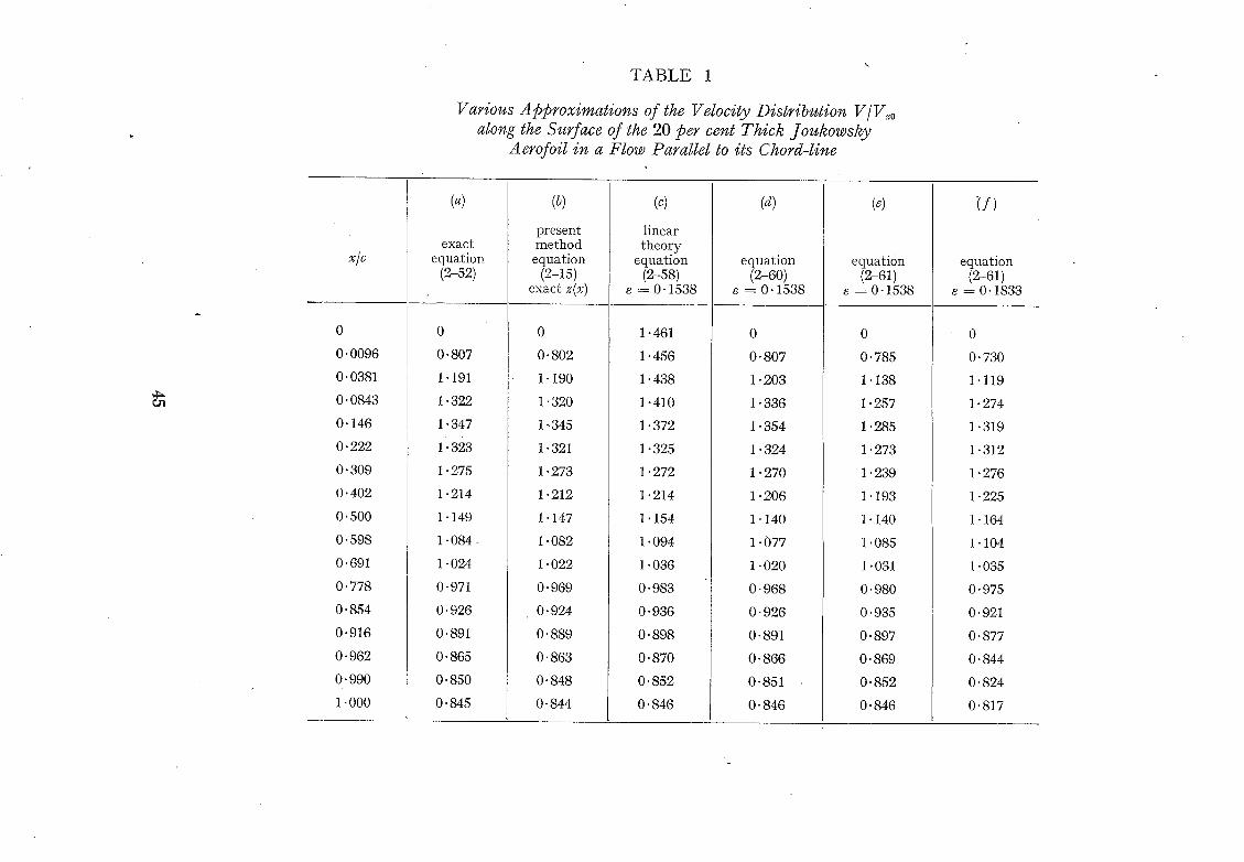
T A B L E 1

Various Approximations of the Velocity Distribution V/V,o along the Surface of the 20 per cent Thick Joukowsky

A erofoil in a Flow Parallel to its Chord-line

x/c

0

0 .0096

0.0381

0.0843

0 .146

0 .222

0 .309

0 .402

0 .500

0 ,598

0.691

0 .778

0.854

0-916

0 .962

0.990

1.000

(a)

exact equat ion

(2-52)

(b)

present me thod

equat ion (2-15)

exact z(x)

(c)

l inear theory

equa t ion (2-58)

s = O. 1538

(d)

equa t ion (2-60)

e = O- 1538

(~)

equation (2-61)

e = 0 - 1 5 3 8

0 0

0.807 0-802

1.191 1-190

1.322 1.320

1-347 1,345

1-323 1-321

1.275 1-273

1.214 1.212

1.149 1.147

1 .084- 1.082

1.024 1-022

0.971 0.969

0.926 0.924

0.891 0.889

0.865 0 .863

0.850 0 .848

0.845 0-844

1.461

1.456

1.438

1.410

1. 372

1.325

1.272

1.214

1. 154

1.094

1.036

O. 983

O. 936

O. 898

O. 870

O. 852

O. 846

0

O- 807

1 • 203

1 • 336

1.354

1- 324

1 • 270

1 .206

1-140

1 • 077

1- 020

O- 968

O. 926

O. 891

O- 866

0-851

O- 846

0

O. 785

1. 138

1.257

1.285

1.273

1.239

1.193

1.140

1.085

1.031

O. 980

O. 935

O. 897

O. 869

0 .852

O. 846

i f )

equation (2-61)

e = O. 1833

0

0.730

1.119

1- 274

1.319

1.312

1.276

1.225

1.164

1.104

1.035

O. 975

O" 921

0-877

O- 844

O" 824

0.817

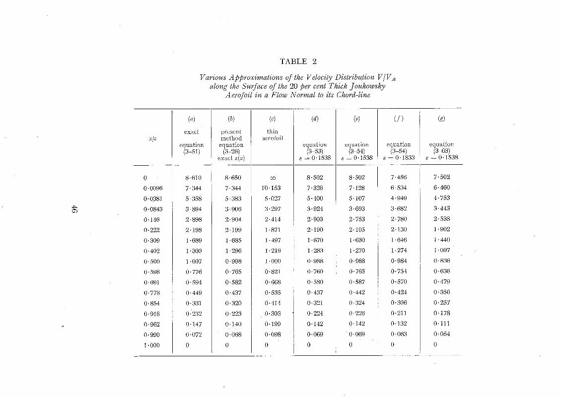
T A B L E 2

Various Approximations of the Velocity Distribcttion V/V,o along the Surface of the 20 per cent Thick Joukowsky

A erofoil in a Flow Normal to its Chord-line

0

0.0096

0.0381

0.0843

0-146

0.222

0.309

0.402

0.500

0.598

0.691

0.778

0.854

0.916

0"962

0-990

1"000

(~)

exact

equat ion (3-51)

(t)

present method

equat ion (3-26)

exact z(x)

(c)

th in aerofoil

(d)

equat ion (3-53)

e=0-1538

(e)

equation (3-54)

s = O" 1538

( f )

equat ion (3-54)

s = O. 1833

8.610

7-344

5.358

3-894

2-898

2-198

1.689

1-303

1.007

0-776

0.594

0-449

0-331

0.'232

0.147

0.072

0

8-650

7-344

5.383

3.906

2-904

2.199

1.685

1-296

0.998

0-765

0"582

0"437

0"320

0-223

0-140

0-068

0

O9

10.153

5.027

3.297

2.414

1.871

1"497

1"219

1"000

0"821

0"668

0"535

0.414

0-303

0"199

0"098

0

8.502

7.326

5.400

3.924

2.903

2.190

1.670

1.283

0.988

0.760

0.580

0.437

0.321

0.224

0.142

0.069

0

8" 502

7" 128

5" 107

3" 693

2" 753

2" 105

1-630

1" 270

O" 988

O" 765

0.587

0.442

0- 324

0.226

0.142

0.069

0

7" 456

6- 534

4" 949

3" 682

2- 780

2- 130

1- 646

1" 274

O" 984

0-754

O- 570

O- 424

O" 306

0.211

O" 132

O" 063

0

(g)

equat ion (3-63)

s = O" 1538

7. 502

6.460

4. 753

3.443

2. 538

1 • 902

1. 440

1. 097

O- 836

O. 636

O. 479

O. 356

O. 257

O" 178

0.111

O" 054

0

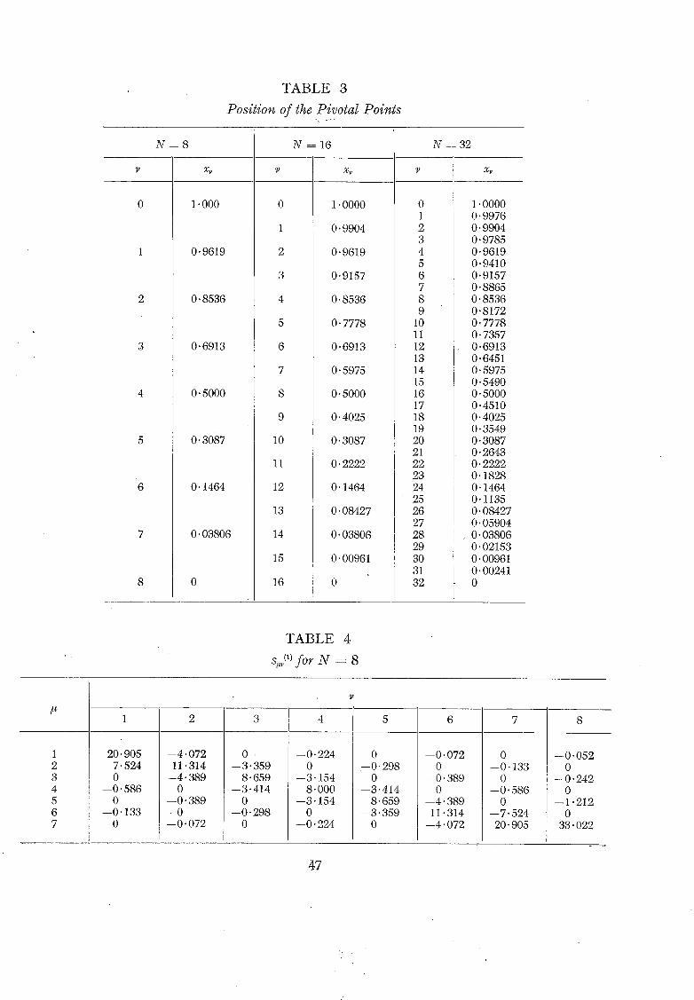
TABLE 3

Position of the Pivotal Points

0

4

"6

8

N = 8

x~

1-000

0.9619

0.8536

0.6913

0.5000

0-3087

0.1464

0.03806

0

1

2

3

4

5

6

7

8

9

10

11

12

13

14

15

16

1.0000

0.9904

0.9619

0.9157

0.8536

0-7778

0.6913

0.5975

0.5000

0.4025

0.3087

0.2222

0.1464

0.08427

0.03806

0.00961

0

0 1 2 3 4 5 6 7 8 9

10 11 12 13 14 15 16 17 18 19 20 21 22 23 24 25 26 27 28 29 3O 31 32

N = 1 6 N = 32

1.0000 0.9976 0.9904 0.9785 0.9619 0.9410 0.9157 0.8865 0.8536 0.8172 0.7778 0.7357 0.6913 0.6451 0.5975 0.5490 0.5000 0.4510 0.4025 0.3549 0.3087 0.2643 0.2222 0.1828 0.1464 0.1135 0.08427 0.05904 0.03806 0.02153 0.00961 0.00241 0

TABLE 4

s~ (1) for N = 8

# 1 2 3 4 5 6 7 8

1 2 3 4 5 6 7

20.905 - - 7 . 5 2 4

0 - - 0 . 5 8 6

0 - - 0 . 1 3 3

0

- - 4 . 0 7 2 11.314

- - 4 . 3 8 9 0

- - 0 . 3 8 9 0

- - 0 - 0 7 2

0 "

- - 3 . 3 5 9 8 .659

- - 3 . 4 1 4 0

- - 0 - 2 9 8 0

- - 0 . 2 2 4 0

- - 3 . 1 5 4 8-000

- -3 -154 0

- - 0 . 2 2 4

0 : - 0 ' 2 9 8

0 - - 3 . 4 1 4

8-659 - -3 -359

0

- - 0 . 0 7 2 0

- - 0 . 3 8 9 0

- - 4 . 3 8 9 11.314

- -4"072

0 - -0 -133

0 - - 0 . 5 8 6

0 - - 7 . 5 2 4 20.905

- - 0 . 0 5 2 0

- -0 .242 0

- - 1 . 2 1 2 0

- -33 . 022

47

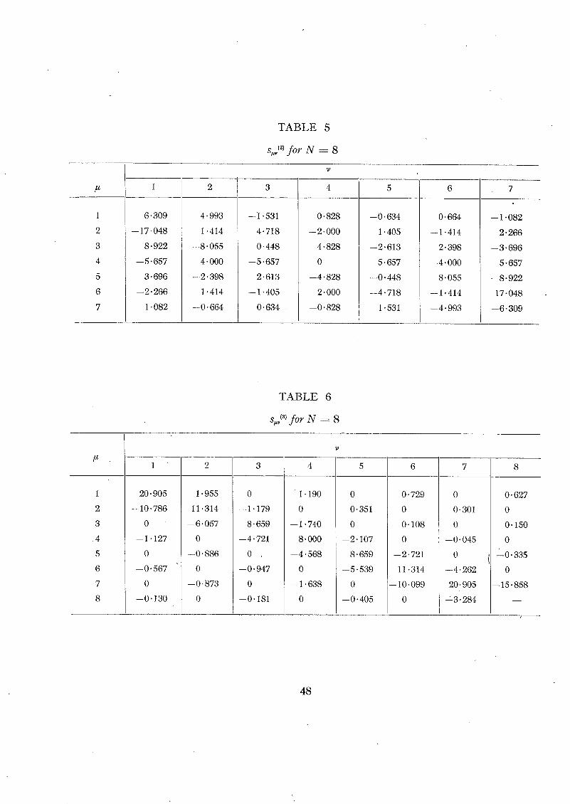
TABLE 5

s~v ~2) f o r N = 8

# 1 2 3 4 5 6 7

1

2

3

4

5

6

7

6.309

--17"048

8-922

--5 .657

3.696

- -2 .266

1.082

4-993

1.414

--8"055

4.000

- -2 .398

t .414

--0.664

--1.531

4.718

0.448

--5 .657

2.613

--1 .405

0.634

0.828

- -2 .000

4.828

0

- -4 .828

2.000

- -0 .828

--0.634

1.405

--2 .613

5.657

--0 .448

--4 .718

1.531

0.664

--1.414

2.398

- -4 .000

8.055

--1 ,414

--4 .993

- -1 .082

2.266

--3 .696

5.657

- -8 .922

17-048

--6-309

TABLE 6

s., (3) f o r N = 8

1

2

3

4

5

6

7

8

20.905

--10.786

0

1.955

11-314

- -6 .057

0

--1.179

8.659

1 . 1 9 0

0

- -1 .740

0

0"351

0

0.729

0

0.108

0

0- 301

0

- -1 .127

0

--0"567

0

--0"130

0

- -0 .886

0

- -0 .873

0

--4.721

0

- -0 .947

0

--0.181

8.000

- -4 .568

0

- -1 .638

0

- -2 .107

8"659

--5"539

0

--0"405

0

--2.721

11.314

--10.099

0

- -0 .045

0

- -4 .262

20.905

--'3.284

8

0-627

0

0-150

0

- -0 . 335

0

--15-858

48

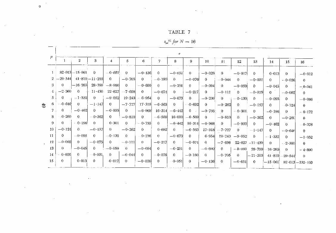
T A B L E 7

s.~ (1) f o r N = 16

2 3 4 5 6 7

~J

8 9 10 11 12 13 14 If 16

1

2

3

4

5

6

7

8

9

10

11 0

12 - -0 .062 i

13 0

14 - -0 .026

15 0

- -15 .061 0 - -0 .651 0

4 1 . 8 1 0 - - 1 1 . 2 0 3 0 - -0 -705

- -16 .265 28.799 --8.9813 0

0 - - 1 1 . 4 3 0 22.627 - -7 .698

- -1 .532 0 - -9 .052 19.243

0 - -1 -147 0 - -7 -727

- -0 .462 0 - - 0 . 9 3 5 0

0 - -0 .362 0 --0.8113

- -0 -196 0 - -0 .301 0

0 - - 0 . 1 5 7 0 - - 0 . 2 6 2

- -0 .095 0 - - 0 . 1 3 0 0

0 - -0"075 0 - -0 .111

- -0 .045 0 --0.059 0

0 --0.031 0 --0-044

--0"013 0 --0.017 0

- - 0

0

- - 0 "

0

- - 6 "

17.

- - 6 "

0

- -0 .735

0

- - 0 . 2 3 (

0

- - 0 . 0 9 4

0

- - 0 . 0 2 (

136 0

- -0 .180

69G 0

0.674

954 0

318 - -6 .563

9681 16-314

- - 6 . 569

0

- -0 .692

0

- -0 .217

0

- -0"076

0

--0"051 0 - - 0 . 0 2 6 0

0 - - 0 . 0 7 6 0 - - 0 . 0 4 4

- -0-201 0 - - 0 . 0 9 4 0

0 - -0 .217 0 - -0"111

- -0 .673 0 - - 0 . 2 3 6 0

0 - -0 .692 0 - -0"262

- -6 .442 0 - - 0 . 7 3 5 0

16.000 - -6 .569 0 - - 0 . 8 1 0

- -6 .442 16.314 - -6"968 0

0 - -6"563 17"318 - - 7 . 7 2 7

- -0 .673 0 - -6 -954 19.243

0 - -0 .674 0 - -7"698

- -0 .201 0 - - 0 . 6 9 0 0

0 - -0"180 0 - -0"705

--0"051 0 --0'1361 0

- - 0 . 0 1 7 0 - -0 -018 0

0 - -0 . 031 0 - - 0 .

- - 0 . 0 5 9 0 - -0 .045 0

0 - - 0 . 075 0 --0"

- - 0 . 130 0 - -0 .095 0

0 - - 0 . 1 5 7 0 - - 0 .

- -0 .301 0 - - 0 - t9~ 0

0 - -0 . 362 0 - - 0 .

--0" 935 0 --0. 462 0

0 --I. 147 0 --0.

--9.052 0 --I .532 0

22.627 --Ii .430 0 --2.

--8. 980 28. 799-- 16.265 0

0 --11-203 41.81G--29.

- -0 .651 0 - -15 "061 82.

- -0 .012

02C 0

_0"041

062 0

- -0"08~

124 0

- - 0 . 172

2613 0

- -0 . 378

64~ 0

- - 1.052

3613 0

--4.89C

544 0

013 - -132. 103

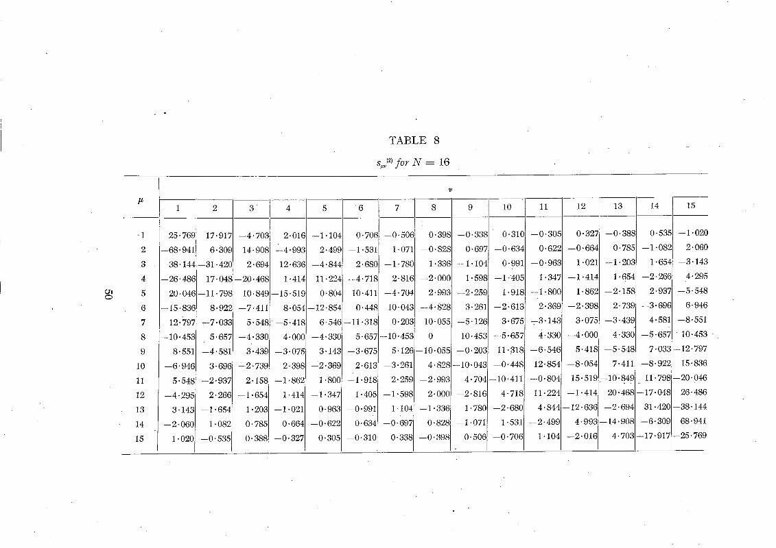
TABLE 8

s~ C~l f o r N -~ 16

# 1 2 3 4 5 6 7 8 9 10 11 12 13 14 15

-1

2

3

4

5

6

7

8

9

10

11

12

13

14

15

25.76g 17-917 --4.703 2.016 --1.104 0.706 --0-506 0.398 --0.338 0-310 --0.305 0.327 - -0 .388 0.535 - -1 .020

--68.941 6.30~ 14-908 --4-993 2.499 l l - 5 3 1 1.071 --0-828 0.697 --0.634 0.622 --0-664 0.785 --1.082 2-060

38 .144- -31 .420 2.694 12.636 --4.844 2.680 --1.780 1.336 --1.104 0.991 --0.963 1-021 --1.203i 1.654 13 .143

- -26 .486 17.048--20.468 1.414 11.224 --4.718 2.816 --2 .000 1.598 --1.~05 t .347 --1.4141 1.654 12 .266 4.295

20 .046--11 .798 10.84g--15.519 0.804 10.411 --4.704 2.993 --2-259 1.918 --1 .800 1.862! --2.158 2.937 --5 .548

--15.83E 8.922 --7.411 8.054--12"854 0"448 10-043 --4"828 3"261 --2.613 2"369 --2"398 2"73g --3.696 6-946

12.795 =-7"033 5"548!--5"418 6"546--Ii'318 0.203 10"055 --5"126 3.675 =-3"143 3"075 --3"439 4"581 --8"551

--10-453 5"657 --4.330 4"000 --4"330 5.657--10"453 0 10"453 --5"657 5-330 --4.000 4-330 --5-657 10.453

8"551 --4"581 3"439 --3"075 3"143 --3"675 5.126--10"055 --0"203 11"318 --6.546 5.418 --5"548 7"033 -12.797

--6"946 3-696 --2"739 2-398 ±2"369 2"613 --3.261 4.828--10"043 --0"448 12-854 --8.054 7.411 --8-922 15"836

5"548 --2"937 2"158 --1"862 1.800i --1"918 2.259 --2.993 4-704--I0"411 --0"804 15"519--10"849 !1"798--20"046

--4"295 2"266 --1-654 1"41.4 --1"347 1-405 --1"598 2.000 --2-816 4.718--11-224 --1"414 20.468--17"048 26"486

3"143 --1-654 1-203 --1.021 0"963 --0"991 1"104 --1.336 1-780 --2-680 4.844--12"636 --2.694 31.420 144

--2.060 1.082 --0.785 0"664 --0.622 0"634 --0"697 0.828 --I'0711 1"531 --2"499 4-993--14.908 --6.309 68:941

1"020 --0"535 0-388 --0"325 0"305 --0"310 0"338 --0.398 0"50E --0-70~ 1.104 --2"016 4.703--17.917--25"769

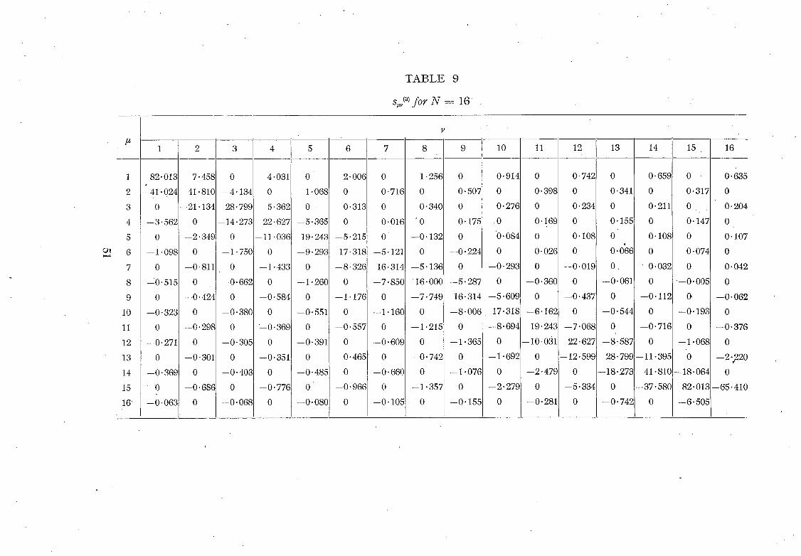
T A B L E 9

s., (3) f o r N = 1 6

1

2

3

4

5

6

7

8

9

10

11

12

13

14

15

16'

1

• 82.013 7-458

-41.024 41.810

0 21.134

--3.562 0

0 -2.349

--1.098 0

0 -0.811

--0-515 0

0 -0.424

--0-323 0

0 -0.298

--0.271 0

0 -0"301

--0.3691 0

' 0 -0.68E

- -0 .063 0

0

--4.134

28.799

-14-273

0

- 1 - 7 5 0

0

--0.662

0

--0.380

0

--0.305 0

--0.403 0

--0.068

4 5

4-031 O

0 1.06~

5.362 0

12.627 --5.365

1.036 19.24~

0 --9.29~

1.433 0

0 --1.26fi

0.584 0

0 --0-551

0.369, 0

0 --0.391

0.351 0

0 --0.48~

0.776 O

0 --0.08(

6

2 -006

~ .068

--5.365 ~.313

19.243 --5.215

- 9 . 2 9 3 1 i7.318!

0 --8.326

--1.260 0

0 --1"176 !

--0-551 0

0 --0.557

--0.391 0

0 --0.465

--0.485 0

O --0.966

--0.080 0

:716 1216 ( :3 o :°16 : 32 5. 121

6. 314 --5- 136

16-000

0.105, -;'357/

9

0

~ .507

~ .175

--~.224 --5.287

--:.365

--~.076]

/

10

0.914

0

0.276

0

'0.084

0

--0.293

0

--5.609

17.318

--8.694

0

--1.692

0

--2-279

0

11 12 13 14

0 0"742 0 0-65£

0-398 0 0"341 0

0 0"234 0 0"211

0 .169 0 01155 0

• ° O-lO8 o . O.lO8

0.026 0 0.066 0

0 --0.019 O, 0 . 0 3 2

--0.360 0 --0.061 0

0 --0.437 0 --0.112

--6.162 0 --0.544 0

19.243 --7"068 0 --0.716

--10"031 22"627 --7-587 0

0 --12"599 28.799--11.395

--2"479 0 --18-273 41.810

--~.2811 --~-334 __~.7421--3~.580

15

.

0.317

0 , •

O. 147

0

O. 074

0

- - 0 . 0 0 5

O.

--0" 19~

0

--1.06~

0

--18.064

82.01,~

--6.50~

16

0.635

0

0. 204

0

0" 107

0

0. 042

0

- - 0 . 0 6 2

0

- - 0 . 3 7 6

0

-2.g2o 0

--65.410

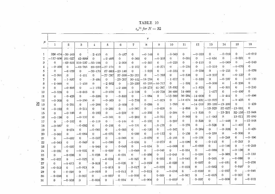
T A B L E 10

s.~(1! for N = 32

# 1 2 3 4 5 6 7 8 9 10 11 12 13 14 15 16

6

7

8

9

10

11

12 O1 t,~ 13

14

15

16

i7 18

19

20

21

22

23

24

25

26

27

28

29

30

31

326.474--59.103 0

--117.63E 164.027--42.889

0 --63.816

--9.40~ 0

0 --6.029

--2"591 0

0 --1.837

--1"065 0

0 --0"805

-o.5381 o 0 --0.425

--0.30S 0

0 --0.251

--0.192 0

0 --0-160

--0.12~ 0

0 --0.107

--0.087 0

0 --0.074

--0-061 0

0 --0.052

--0-043 0

0 --0.037

--0.031 0

0 --0.02~

--0.021 0

0 --0.017

--0.013 0

0 --0.010

--0.006 0

0 --0-003

- -2-410 0

0 - -2 .495

110.237--33.198 0

--43.765 83.620--27.171

0 --33.470

--4.411 0

0 - -3 .484

- -1 .416 0

0 - -1-153

--0-645 0

0 - -0-538

- -0 .350 0

0 - -0-298

--0.211 0

0 - -0 .182

--0 .137 0

0 - -0 .119

- -0 .092 0

0 --0.081

--0 .064 0

0 - -0-057

--0.045~ 0

0 - -0 .040

--0.032 0

0 - -0-028

--0.022 0

0 - -0 .018

--0 .013 0

0 - -0 .010

- -0 .007 0

9 - -0 .003

--0.457 0 --0.148 0 --0.063 0 - -0 .033 0

0 --0.565 0 --0-203 0 --0.094 0 - -0 .051

--2.305 0 --0-581 0 --0.225 0 - -0 .110 0

0 - -2 .102 0 --0.571 0 --0.234 0 - -0-119

67.883--23.149 0 --1.928 0 --0.553 0 - -0 .236 0

--27.287 57.599--20.321 0 --1.788 0 --0-536 0 - -0-237

0 --23-207 50.442--18.25S 0 --1-677 0 - -0 .520 0

--2-892 0 --20-350 45.255--16.717 0 --1"591 0 - -0 .509

0 - -2 .488 0 --18.275 41.397--15.552 0 - -1-525 0

--0-97( 0 --2"198 0 - -16.728 38.486--14.669 0 - -1 .477

0 - -0 .850 0 --1.984 0 --15.560 36.284--14.0081 0

--0-463 0 - -0 .758 0 --1.823 0 --14.674 34 .637 - -13 .527

0 --.0.408 0 --0.688 0 --1-700 0 --14.010

- -0 .260 0 --0.367 0 --0.635 0 - -1 .606 0

0 --0.231 0 --0.335 0 --0.594 0 --1"535

--0.161 0 --0.209 0 --0.311 0 - -0 .563 0

0 - -0 .144 0 --0.192 0 --0.291 0 --0"538

- -0 .106 0 --0.131 0 =0.178 0 - -0 .276 0

0 --0.095 0 --0.120 0 --0.167 0 - -0 .264

- -0-072 0 --0.086 0 --0.112 0 - - 0 . 1 5 8 0

0 --0.065 0 --0.079 0 --0.105 0 - -0 .151

- -0 .050 0 - -0 .059 0 --0.073 0 - -0 .099 0

0 --0.045 0 --0.054 0 --0.068 0 - -0 .093

--0-035 0 --0.040 0 --0.049 0 --0.064 0

0 --0.031: 0 --0.036 0 --0.045 0 - -0 .059

- -0 .024 0 --0.027 0 --0.032 0 --0-041 0

0 --0-02C 0 " --0.023 0 --0.029 0 - -0 .037

--0-015 0 --0.017 0 --0.020 0 --0-025 0

0 --0.011 0 --0.013i 0 -O.O1e 0 - -0 .020

--0-007 0 --0-008 0 --0.009 0 --0.012 0

0 --0-004 0 --0.004 0 --0.005 0 - -0 .007

--0"019 0 --0"012

0 --0.031 0

- -0 .063 0 --0-04C

0 --0-07C 0

--0.1251 0 --0-07G

0 --0.129 0

--0.237 0 --0.133

0 --0.238 0

--0.501 0 --0.240

0 --0.496 0

- -1 .444 0 --0.496

0 --1-425 0

33 .440- -13 .199 0 --1-420

- -13 .529 32-627--13.010 0

0 --13-201 32.155--12.948

- -1 .483 0 --13-011 32.000

0 - -1 .448 0 --12.948

- -0 .520 0 --1-427 0

0 - -0 .508 0 - -1 .420

- -0 .255 0 --0-500 0

0 - -0-248 0 - -0 .496

- -0 .145 0 - -0 .243 0

0 - -0 .140 0 - -0 .240

- -0 .089 0 - -0"136. 0

0 - -0-085 0 --0-133

- - 0 . 0 5 5 0 - -0 .080 0

0 --0.051 0 - -0 .076

- -0 .032 0 --O.04E 0

0 - -0 . 027 0 - -0 .040

- -0 .015 0 - -0 '021 0

0 --0-00~ 0 - -0 .012

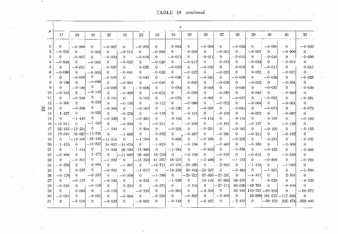
18

10 11 12

ol 13 5¢

14

15

16 17

18

19

20 21

22

23 24

25

26

27

28 29

30

31

# 17

1 0

2 --0 .021

3 0

4 - -0"046

5 0

6 - -0 .080 7 0

8 - -0 .136

9 0

- -0 .243

0 - -0 .500

0

- -1 .427

0 -13.011

32.155

-13.010

0

- -1 .425

0

--0"496

0 - -0 .238

0

--0" 129

0

--0. 070

0

--0"031

0

19 I

- -0 .009 0

- -0 .027

0 - -0 .051

0

- -0 .085

0 - -0 .140

0 - -0 .248

0 - -0 . 508

0

- -1 .448

0

-13.201

32.627

-13.199

0

- -1 .444

0 --0.501

0

- -0 .237

0 - -0 .125

0

- -0 .063

0

- -0 .019

i

2O i

0 --0.0151

0

- - O- 0321 0 i

- -0 .055 0

--0.089

0

- -0 .145

0

- -0 .255

0

- -0 .520

0

- -1 .483

0 -13 .529

33.440

-13"527

0

- -1 .477

0

- -0 . 509

0 - -0 .237

0 - -0 .119

0

- -0 . 051

0

- -0 .007

0 - -0-020

0 --0" 037

0 --0.05c~

0

T A B L E lO--continued E

- 2 1 , 2 2 2 3

o - 0 . 0 0 5 o --0"0121 0 - -0"009 !

0 --0.0161 0 --0.025] 0 - -0 .020

0 --0.0291 0 --0.0411 0 - -0 .032

0 --0-045i 0

--0.0641 0 - -0 .049

24 25

--0.004[ 0

0 ] - -0 .008

--0.013[ 0 ", 0 [ ' - - 0 . 0 1 7

--0"023[ 0

0 I - -0 -027

--0.0361 0

? I -0.040 0

- -0 .059

0 - -0 .086

0

- -0 .131

0

- -0 .209

0

- -0 .367

0

- -0 .758

0 - -2 .198

0 -20 .350

50.442

-20.321

0

- -2 .102

0

- -0 .565

0

26

--0"004:

--0"011]

0

- -0"020

--0.0311

- -0 .045

0 - -0 .065

0

- -0 .095

0 - -0 .144

0

- -0 .231

0

- -0-408

0

- -0 .850

0 - -2 .488

0

--23"207

57"599

23"149

0

- -2"305

0

- -0"457

7 - -

- -~-007

28 29 " 3 0

--0"0031 0 - -~-003 - -0"007

--0"0101 0 --0.010t

- -0-015 t - -0 .013 - -~ .017 0 - -0 .0181 0

--0-024 - -0 .022 0 [

0 --0.0281 0 - -0 .026

o - -0 .035 - -0 .0 3 2

0 - - 0 . 0 4 0 1 0 - -0 .037

--0.0501 - -0 .045 --0.0520 - -0 .0 4 3 0 --0.0571 0 0

- -0 .072 - -0 .064 0 - - 0 . 0 6 1

0 --0.081l 0 - -0 .074 0

--0.10C - -0 .092 0 - -0 .0 8 7

0 --0.119l 0 - -0 .107 0

--0-161 - -0 .137 0 - -0 .126 0 --0.182l 0 - -0 .160 0

--0-2601 --0-211 0 - -0 .1 9 2

0 --0"298t 0 - -0 .251 0

- -0 .463 - -0 .350 0 - -0 .3 0 8 0 --0"538] 0 - -0 .425 0

--0.976i - -0 .645 0 - -0 .538

0 - -1 .153 0 - -0"805 0

--2"8921 0 - -1 .416 0 - -1 .065 I

0 J - -3 .484 0 - -1 .837 0

- -27.287 --4 .411 0

67.883--33.470l 0 - -6 .029 - -27.171 83 .620 - -43 .765 0

0 - - 3 3 . 1 9 8 1 1 0 . 2 3 7 - - 6 3 . 8 1 6 --2 .495 - - 4 2 . 8 8 9 1 6 4 . 0 2 7

0 --2.410] 0 - -59 .103

31 32

0 - - O. 003 - -0 .0 0 ( 0

0 - - 0 . 0 0 9

- -0 -013 0

0 - -0 .017 - -0 .021 0

0 - -0 .0 2 5 - -0 . 031 0

0 --0" 036

0

--0"051

0 - -0 .0 7 2

0

- -0 . 103 0

- -0 . 153 0

- -0 .237

0

- -0 . 395 0

--0" 723 0

- - 1. 539

- -2 .591 0

0 - -4 .2 2 6 - -9 .409 0

0 - -19 .572

- - 117.63(~ --520"8 326" 474 400

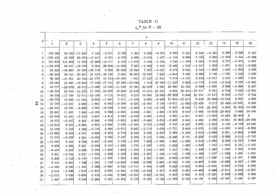
TABLE 11 s,~ (2) f o r N = 3 2

# 1 2 3 4 5 6 7 8 9 10 11 12 13 14 15 16

1 103.586 69"783--17"658 7-184 --3"671 2.155 --1.391 : 0.962 --0-703 0.53~ --0.424 0.346 --0.291 0.250 --0.220 0-197

2 --276.452 25.769 56-370--17-917 8.372 --4-703 2.960 --2.016 1.457 --1-104 0.869 --0 .706 0.590 --0.506 0.444 --0-398

3 154-876--124.802 11.356 45.888--16.417 8.329 --4.976 3.286 --2.328 1.74C --1.356 i .094 --0-910 0.777 --0.679 0.607

4 --109.508 68.941--79.750 6.309 38.696--14.908 7.997 --4.993 3.420 --2.499 1.918 --1-531 1-262 --1.071 0.931 --0.828

5 84.923 --48.880 43.293=-58.716 3.969 33.636--13.645 7.627 --4.927 3.474 --2.604 2"044 --1.665 1.400 --1.209 1.069

6 --69.243 38"144--30-507 31.420--46.720 2.694 29.961i--12.635 7.293 --4.844 3.499 --2.680 2.146 --1.780 1.522 --1.336

7 58-263 --31.301 23.764--21"976 24.713--39.066 1:921 i 27.227--11.841 7.018 --4.770 3.518 --2.747 2.238 --1-889 1.641 8 --50.084 26.487--19.~500 17.048--17.161 20.469--33.82E 1.414 25-160--11.224 6.803 --4 .718 3.546 --2.816 2.333 --2-000

9 43.717 --22,878 16.512--13-956 13-250--14.120 17.581--30.069 1.062 23-589--10.755 6.648 --4.695 3.588 --2.896 2-437

10 --38.592 20.046--14.273 11.798--10-809 10.849--12.055 15-519--27.292 0.804 22-401--10-411i 6-551 --4-704 3-652 --2-993

11 34.356 --17.749 12-514:--10"186 9-115 --8-8171 9.218:--10.583 13.999--25.202 0.606 21.521--10.177 6-509 --4.747 3.742

ca 12 --30"778 15.836--11:084 8.922 --7.851 7-411[I --7.462 8"055 --9"496 12.854--23.617 0.448 20-898--10-043 6-522 --4-828

~. 13 27.700 --14.207 9.890 --7.893 6-862 --6.3651 6.25C --6-493 7-195 --8.677 11-982--22.42C 0.317 20.499--10"002 6.593 14 --25.013 12-797 --8.866 7.033 --6.059 5-548 --5.35C 5.418 --5-776 6.545 --8.050 11.318--21-533 0.203 20.305--10.055

15 22.634 --11.557 7.983 --6.298 5-386 --4.885 4.648 --4-621 4.800 --5.232 6.044 --7.56~ 10-818--20-905 0"099 20.306

16 --20.503 t0.453 --7.200 5.657 --4-811 4.3301 --4-078 4.000 --4"078 4.330 --4-811 5.657 --7-200 10.453--20.503 0 17 18-575 --9.457 6.499 .--5.090 4.309 --3.854 3-602 - -3 "496 3-516 --3.663 3.963 --4.482 5-356 --6.924 10.202--20.306

18 --16.813 8.551 --5.86E 4.581 --3.864 3.439 --3.193 3.075 --3.059 3.142 --3.337 3.675 --4-223 5-126 --6.725 10.055

19 15-190 --7.718 5,286 ~-4.119; 3-464 --3-071 2.837 --2,714 2.678 --2.721 2.849 --3.078 3.445 --4.020 4.953 - -6 .593

20 -- i3-682 6"946 --4.752 3"6961 --3.10C 2-739 --2.520 2.398 --2.350 2-369 --2.453 2.613 - -2 .869 3.261 --3.862 4-828

2 1 12-270 --6.226 4.254 --3"3031 2.7651 --2.437 2.234 --2.117 2.063 --2.066 2-121 ~2 .235 2.420 --2.698 3.113 --3.742

22 --10.940 5-548 - -3 .788 2.937 --2.454 2.158 --1-973 1.863 --1.808 1.800 --1.836 1--918 --2-054 2.259 --2-557 2.993 23 9.679 --4.906 3.347 --2.593 2.163 --1.898 1.732 --1.630 1.576 --1.563 1.585 --1-645 1-747 --1.900 2.121 --2.437

24 --8.476 4.295 --2.928! 2-266 --1.888 1.654 --1.506 1.414 --1.364 1.347 - - t - 36 t 1.405 --1 .482 1.598 --1-765 2.000

25 7.321 --3.708 2.527 --1.954 1.626 --1-423 1.294 --1.212 1.166 --1.149 1.156 --1-188 1.247 --1.336 1-464 --1.641

26 --6.206 3.143: --2.14C 1.654 --1.376 1-203 --1.091 1.021 :-0.981 0-963 --0.967 0-991 --1.035 1.104 --1.201 1.336

27 5.124 --2.594 1.766 --1.364 1.134 --0-990 0.898 --0.839 0.804 --0"789 0.790 --0-807 0.840 --0.893! 0"967i --1,069

28 --4.069 2-06C --1.402 1.082 --0.899 0-785 --0.711 0.664 --0.635 0-622 --0.622 0.634 - -0 .659 0.697 --0.753 0.828

29 3,034 --1.53~ 1.045 --0-807 0.67G --0.584 0.529 --0-493 0.472 --0.462 0.461 --0-469 0.48E --0.514 0.553 --0.607

30 --2.015 1-020 --0.694 0.535 --0.444 0"388 --0.351 0-327 --0.313 0,305 --0.305 0.310 --0.321 0.338 --0~363 0.398 31 1.005 --0.509 0.346 --0.26C 0-222 --0.194 0.175 --0~163 0.156 --0.152 0.152 --0.154 0.159 --0.167 0.18G --0.197

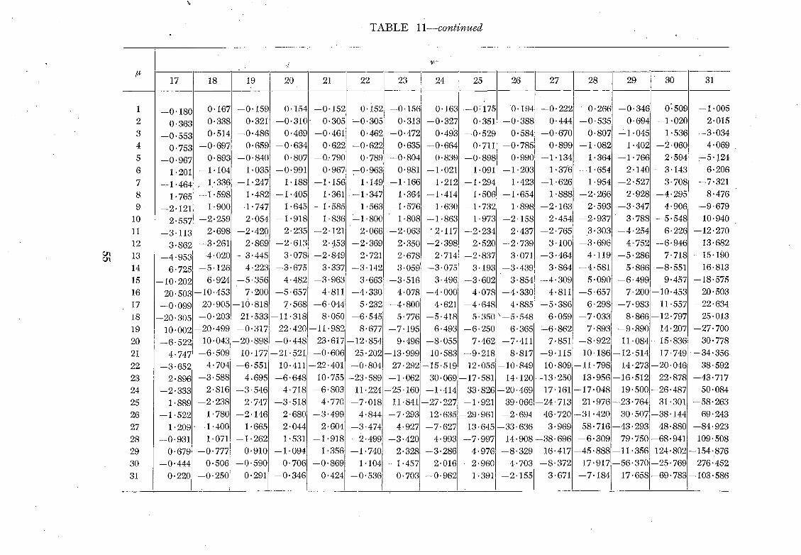
TABLE l l--continued

# 17 18 19 20 21 22 23 24 25 26 27 28 29 30 31

C, gq

5

6

7

8 9

10

11

12

13

14

15

16

17 18

19 20

21

22

23

24 25

26

27

28

29

30

31

--0"180 0"167 --0"159 0.154 --0"152 0.i52 --0.156 0"163 ---0:i75 0.194 --0.222 ' 0.266 --0"34~ 0:509 --1"005

0"363 --0"338 0"321 --0.310 0.305 :--0"305 0.313 --0"327 0"351 --0,388 0"444 --0"535 0"694 --1-020i 2"015

--0.553 0"514 --0"486 0.469 --0.461! 0.462 --0"472 0"493 --0"529 0.584 --0"670 0"807 --1"045 1"53~ --3"034

0.753 --0"697 0.659 --0.634 0.622 --0.622 0.635 --0.664 0"711 --0.785 0.899 --1-082 1.402 --2.060 4"069

--0.967 0.893 --0.840 0.807 --0.790 0.789 --0.804 0.839 --0.898 0.990 --1.134 1-364 --1-76~ 2.594 - -5 . ]24 1.201 --1-104 1.035 --0.991 0.967 --0.963 0.981 --1.021 1.091 --1.203 1-376 --1.654 2.140 ~--3.143 6.206

--1"464 • 1-336 --1.247 1.188 --1.156i 1.149 --1.166 1.212 --1.294 1.423 --1-626 1.954 --2.527 3-708 --7.321

1.765 --1.598 1.482 --1.405 1.361 J--1.347 1.364 --1.414 1.5061 --1-6541 1.888 --2-266 2-928 --4.295 8"476

--2.121 1.900 --1.747 1.645 --1-585 1.563 --1.576 1.630 --1.732 1.898 --2-163 2-593 --3-347 4.906 --9"679

2.557 --2.259 2.054 --1-918 1.83~ '--1.800 1-808 --1.863 1,973 --2.158 2.454 --2-937 3"788 --5"548 10"940

--3.113 2.698 --2.420 2.235 --2.121 2-066 --2.063 "2-I17 ---2.234 2.437 --2.765 3.303 --4.254 6.226 --12.270

3.862 --3.261 2.869 --2-613 2.453 --2-369 2"350 --2.39~ 2.52C --2.739 3-100 --3~696 4-752 --6-946 13.682

--4"953 ,4.020 --3.445 3"07~ --2.849 2.721 --2.678 2.714 --2.837 3.071 --3.464 4-119 --5.286 7"718 --15.190

6-725 --5.126 4.223 --3.675 3-337 --3.142 3.059' --3.075 3.193 --3.439 3-864 --4.581 5"866 --8"551 16.813

--10"202 6.924 --5"356 4"482 --3"963 3-663 --3.516 3"49~ --3.602 3.854 --4"309 5"090 --6"499 9:457 --18.575

20.503--10"453 7.200 --5"657 4"811 --4"330 4.078 --4"000 4.078 --4"330 4"811 --5"657 7"200--10"453 20"503

--0-099 20.905--10-818 7"568 --6"044 5"232 --4.800 4-621 --4.648 4"885 --5-386 6"298 --7-983 11"557 --22"634 --20"305 --0"203 21-533--11-318 8"050 --6-545 5.776 --5"418 5.350 \ - -5 .548 6"059 --7"033 8"866--12"797 25"013

10.002--20"499 --0"317 22.420--11"982 8"677 --7.195 6"493 --6,250 6"365 :-6"862 7"893 --9"890 14.207 --27.700

--6"522 10"043--20-898 --0"448 23"617--12.854 9.49( --8"055 7.462 --7"411 7"8511 --8"922 11-084--15"836 30"778

4"747 --6"509 10"177--21"521 --0"606 25"202--13.999 10"583 --9.218 8"817 --9-115 10"186--12"514 17"749- -34"356

--3"652 4"704 --6-551 10.411--22"401 --0"804 27"292'--15"519 12"055 --10"849 10"809i--11"798 14"273--20"046 38"592

2"89C --3"58~ 4.695 --6"648 10"755--23.589 --1.062 30.069--17.581 14.120--13-250 13"956--16"512 22"878 --43"717

--2.333 2.81E --3"546 4"718 - -6 '803 11.224--25"160 --1"414 33.826--20.469 17"161--17"048 19"500--26"487 50"084

1-889 - -2 .238 2"747 --3"518 4.770 --7"018 11"841--27.227 --1.921 39.066--24"713 21"976--23"764 31"301 --58"263

--1"522 1"78C --2"146 2"680 --3"499 4"844 --7-293 12"635--29.961 --2"694 46-720--31"420 30"507--38"144 69"243

1.209!'--1"40C 1-665 --2-044 2"604 --3"474 4.927 --7"627 13.645--33-636 --3"969 58"716--43"293 48"880 --84"923

--0"931 1.071 --1"262 1"531 --1"918 2"499' --3.420 4"993 --7.997 14-908--38-696 --6"309 79"750--68"941 109"508

0"679 --0"777 0"910 --1"094 1"356 --1"74C 2.328 --3"286 4"976 --8"329 16"417--45"888--11"356 124"802--154-876

--0"444 0"506 --0"590 0"706 --0"869 1"104 --1.457 2.016 --2-960 4"703 --8"372 17"917--56"370--25"769 276"452

0"220 --0"250 0"291 --0"346 0"424 --0"536! 0.703 --0"962 1.391 --2"155 3"671 --7"184 17"658--69"783--103"586

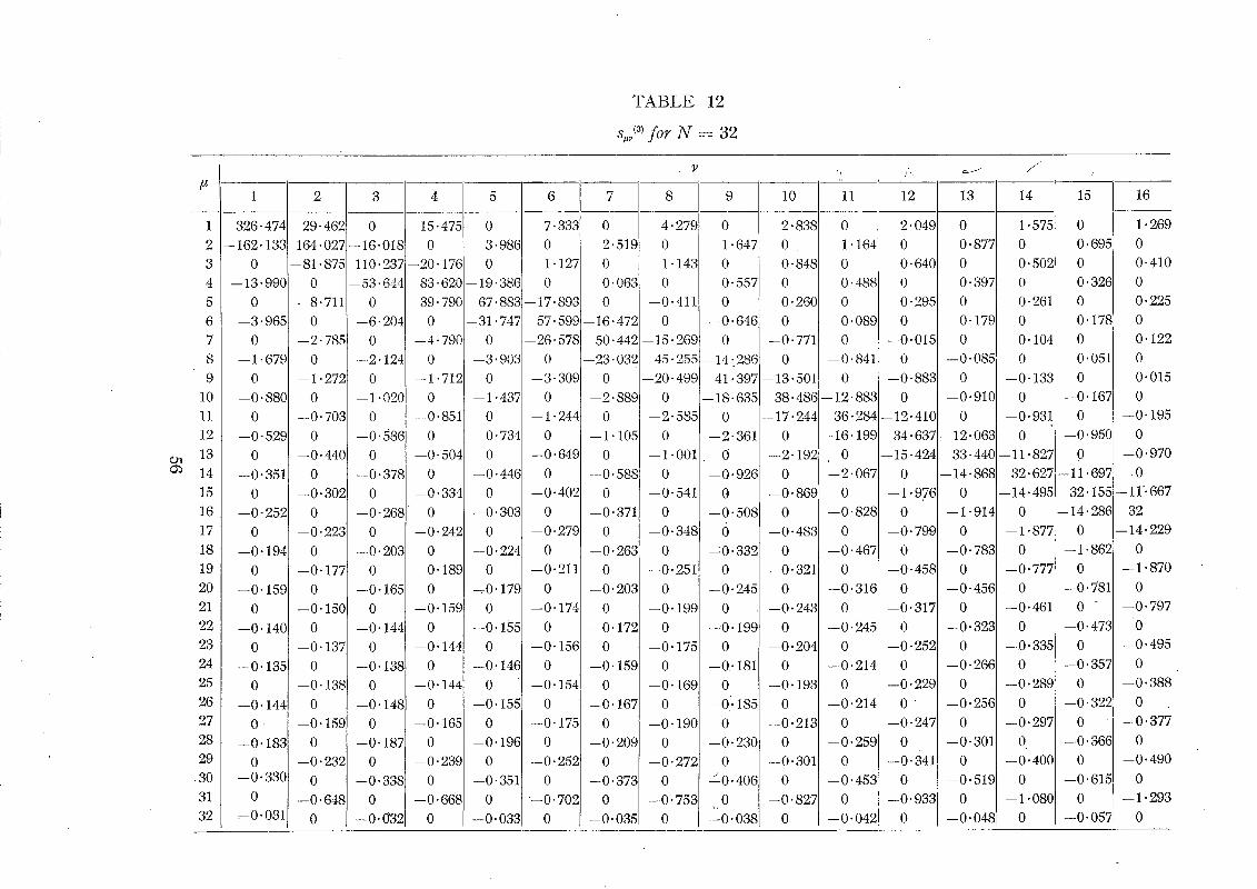
T A B L E 12

s.~ (3) f o r N = 32

6 7

8

9

10 11 12

¢m 13

14

15 16

17

18

19

2O

21 22 23

24 25

26 27

28 29

3 0

31 32

# 1

1 326.474 2 --162.133

3 0

4 --13-990 5 0

--3.965

0 --1.679

0 --0.880

0

--0-529

0 --0.351

0 --0-252

0 --0.194

0 --0.159

0

--0.140

0

--0.135

0

--0.144

0 --0.183

0 --0.330

0 --0.031

0 --8.711

0

0

- -0" 70~

0

- - 0 . 4 4 (

0

0 --0. 177

0

--0.15(

0 --0" 137

0 --0" 13~

0 --0" 15 c

0 --0.23~

0

--0" 648

0

110.2371

--6.2041

--2.1241

- - 1.0201

--0.5861

--0.3781

--0- 2681

--0.2031

--0- 165l

--0- 144] ,,

--0.1381

--0.148]

--0-1871

--0.338[

--0.0321

4 5 6 7

15.475 0 7-333 0

0 3.986l 0 2"5191 -20.176 0 1-127 0

83"620 -19.3861 0 0.0631 -39.790 67.883]-I7 .893 0

0 -31.7471 57.599--16.4721 --4.790 0 -26.578 50.442]

0 --3.903l 0 --23.0321 --1.712 0 --3.309 0

0 --1.437l 0 --2.8891 --0.851 0 --1.244 0

0 --0.734l 0 --1.105l --0-504 0 --0-649 0

0 --0.446l 0 --0.588[

o I - - 0 . 2 4 2

0 --0. 189

0 --0. 159

0 --0. 144

0 --0. 144

0 --0. 165

0 --0.239

0

- - 0 . 6 6 8

0

0 --0.402

--0.3031 0 0 --0.279

-0.2241 0 0 --0.211

~0.1791 0 0 --0.174

--0.1551 0 0 --0.156

--0.146I 0

0 --0-154

--0.1551 0

0 --0.175

--0.1961 0

0 --0.252

--0.351[ 0

0 - -0 .702

--0.033] 0

0 --0.3711

0 - O. 263[

0 --0.2031

0

--0. 1721

0

--0. 1591

0 - - 0 . 1671

0

--0.2091

0 --0.373l

0

--0.0351

b

1.647 0 1.1641

0 0-848 0.557 0 0.4881 0 0.260

--0.646 0 0.089l

0 --0.771

45.255 -14.286 0 --0.841]

-20.499!- 41:397 -13.501

0 --18.635 38.486 -12.8831

12 13

2" 049 0

0 O. 877 0

0 O. 397

0.2951 0 0 O" 17 c

--0.015 0

0 --0-08~

--0.883 0 0 --0.91C

--2-585 0 --17.2441 36-2841--12.410 0

0 --2.361 0 --16.1991 34.637,-12.062

- - 1 . 0 0 1 0 I --2.192 --10.424 33.44C 0 --0.926 0 --2.0671 ~ -14-868

--0.541 0 --0.869 --1.976 0

0 --0.508 0 --0"8281 --1.914

--0.348 0 --0.483 --0.799 0

j ' "

14

.57; 0.502[

0 0.261

0

0.104

0

--0.133

0 --0.931

0 -11.827

32.627

-14.495

--~.877

0

--0.251I

0

--0.199

0

--0-175

0 --0.169

0

--0.190

0 --0.272

0

--0.753

0

--0.332 0

--0.245 0

--0.199 0

--0,.181

0

--0.185

0 --0.230

0 ±0 .406

0

--0.038

0 --0.321

0 --0.243

0 --0.204

0 --0.193

0 --0.213

0

--0.301

0

- - 0 . 8 2 7

0

--0.4671

--0.3161

--0.2451

--0.2141

--0.2141

--0.2591

--0- 4531

--0.0421

0 --0-458

0 --0-317

0 --0.252

0 - - O. 229

O

--0 O- 247

- .341 00.933 _0.048

--0.785 0 0 --0.777

--0.45E 0 0 --0.461

--0-322 0

0 --.0.335

--0.26~ 0 0 --0.289

--0.25~ 0

0 --0.297

--0-301 0 0 --0.400

--0.51 c 0

0 -- 1.080

0

15 16

0 1.269

0.695 0 0 0-410

0.326 0 0 0.225

0.178[ 0

0 0-122

0.051 0

0 0.015

0.167 0 0 --0.195

0.950 0 0 --0-970

- 1.697 0 ;2. 155 --11-667

4.286 32 0 --14-229

1- 8621 0 0 -- 1.870

O. 781 0 0 - --0.797

O- 473 0 0 - - 0 . 4 9 5

0.357 0 0 - - 0 . 388

O. 3221 0 0 --0.377

O. 366 0 0 --0.490

0.615 0 0 -- 1.293

0.057 0

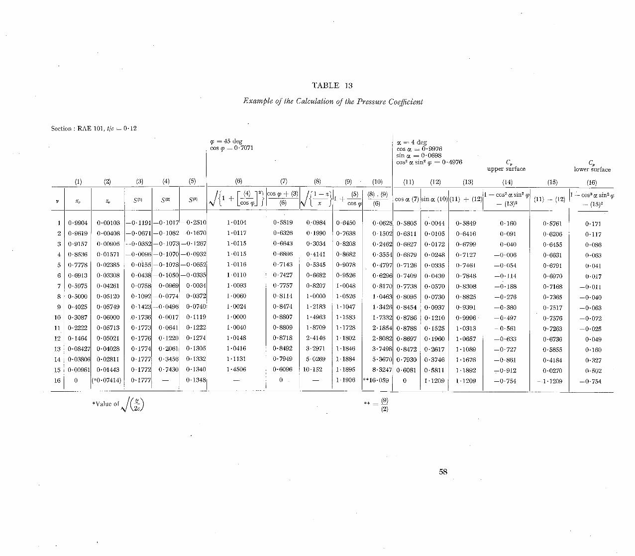
T A B L E 13

Example of the Calculation of the Pressure Coefficient

Section : R A E 101, t/c = 0 .12

(1) (2) (3) (4) (5)

1

2

3

4

5

6

7

8

9

10

11

12

13

14

15

16

x~

0.9904

0.9619

0.9157

0 .8536

0.7778

0.6913

0.5975

0.5000

0.4025

0.3087

0.2222

0.1464

0.08427

0.03806

0.00961

0

z~

0.00103

0.00408

0.00905

0.01571

0.02385

0 .03308

0.04261

0.05120

0"05749

0.06000

0.05713

0.05021

0.04028

0.02811

0.01443

(*0.07414)

S(Z) S(~)

- -0-1191--0-1017

- -0 .0671--0-1082

- - 0 . 0 3 5 2 - - 0 " 1 0 7 3

- - 0 - 0 0 9 6 - - 0 - 1 0 7 0

0 . 0 i 5 5 - - 0 . 1 0 7 8

0 .04381--0-1050

0 . 0 7 5 8 - - 0 . 0 9 6 9

0 - 1 0 9 2 - - 0 . 0 7 7 4

0 . 1 4 2 3 - - 0 . 0 4 9 ~

.0.1736 ) .0017

0-1773 ) '0641

0-1776 ).122G

0 .1774 )-2061

0"1777 ) '345~

0"1772 ) '743C

0"1777 - -

S(s)

- - 0 . 2 5 1 0

- - 0 . 1 6 7 0

- - 0 . 1 2 6 7

- - 0 . 0 9 3 2

- - 0 . 0 6 5 2

0 0335'

0 .0034

0.03721 I

0.07401

0.1119]

0 .1222

0 .1274

0 .1305

0 .1332

0 .1340

0"1348

T = 4 5 deg cos 9 = 0 . 7 0 7 1

(6)

LCOS ~oj d

1.0104

1.0117

1-0115

1-0115

1-0116

1.0110

1.0093

1.0060

1-0024

1.0000

1.0040

1.0148

1.0416

1.1131

1.4506

(7) (8) (9) (10)

cos 9 + (3) (6)

0-5819

0-6326

0.6643

0 .6896

0.7143

0.7427

0-7757

0.8114

0.8474

0 .8807

0 .8809

0 .8718

0 .8492

0"7949

0 .6096

0

cos

0:0984 0.6450

0.1990 0.7638

0.3034 0 .8208

0-4141 0-8682

0.5345 0-9078

0.6682 0.9526

0-8207 1-0048

1.0000 1.0526

1.2183 1-1047

1.4963 1.1583

1.8709 1.1728

2.4146 1.1802

3-2971 1-1846

5.0269 1.1884

10-152 1.1895

1.1906

~ = 4 deg cos a = 0 - 9 9 7 6 sin a = 0 . 0 6 9 8 cos ~ a sin 2 ~ = 0 . 4 9 7 6 G

uppe r surface

(11) (12) (13) (14) (15)

G lower surface

(16)

(8) . (9) (7 ( 6 ) i C O S

0-0628 0-5805

0 .1502 0-6311

0 .2462 0-6627

0-3554 0-6879

0 .4797 0-7126

0 .6296 0-7409

0-8170 0 .7738

1"0463 0 .8095

1.3426 0-8454

1.7332 0 -8786

2. 1854 0 -8788

2 .8082 0-8697

3 .7498 0 .8472

5 .3670 0 .7930

8 .3247 0-6081

* '16"059 0

sin ! ~ (lO)i

0-0044

0 .0105

0 -0172

0 . 0 2 4 8

0 .0335

0 .0439

0 . 0 5 7 0

0 .0730

0 .0937

0 .1210

0 .1525

0 .1960

0 .2617

0 .3746

0 .5811

1 .1209

(11) + (12)

0 .5849

0-6416

0 .6799

0 .7127

0.7461

0-7848

- - ccs ~ ~ sin 2 ~

- (13 )2 (11) - - (12)

0.160

0.091

0 .040

- - 0 . 0 0 6

- - 0 . 0 5 4

- - 0 . 1 1 4

0.5761

0"6206

0.6455

0-6631

0"6791

0.6970

1 L cos 2 ~ sin 2 ,

- ( 1 5 V

0.171

0.117

0 .086

0.063

0"041

0"017

0 . 8 3 0 8

0 .8825

0-9391

0 . 9 9 9 6

1 .0313

1 .0657

1 .1089

1 .1676

1 .1892

1 .1209

- - 0 . 1 8 8

- - 0 . 2 7 6

--0.380

- -0"497

- -0"561

--0-633

- -0"727

- -0 -861

7 0 - 9 1 2

- - 0 - 7 5 4

0.7168

0-7365

0.7517

0-7576

0-7263

0.6736

0.5855

0.4184

0.0270

- - 1 . 1 2 0 9

- -0 .011

- - 0 . 0 4 0

- - 0 . 0 6 3

- - 0 . 0 7 2

- - 0 . 0 2 5

O. 049

O. 160

O. 327

O. 502

- - 0 . 7 5 4

** = (9)

(2)

5 8

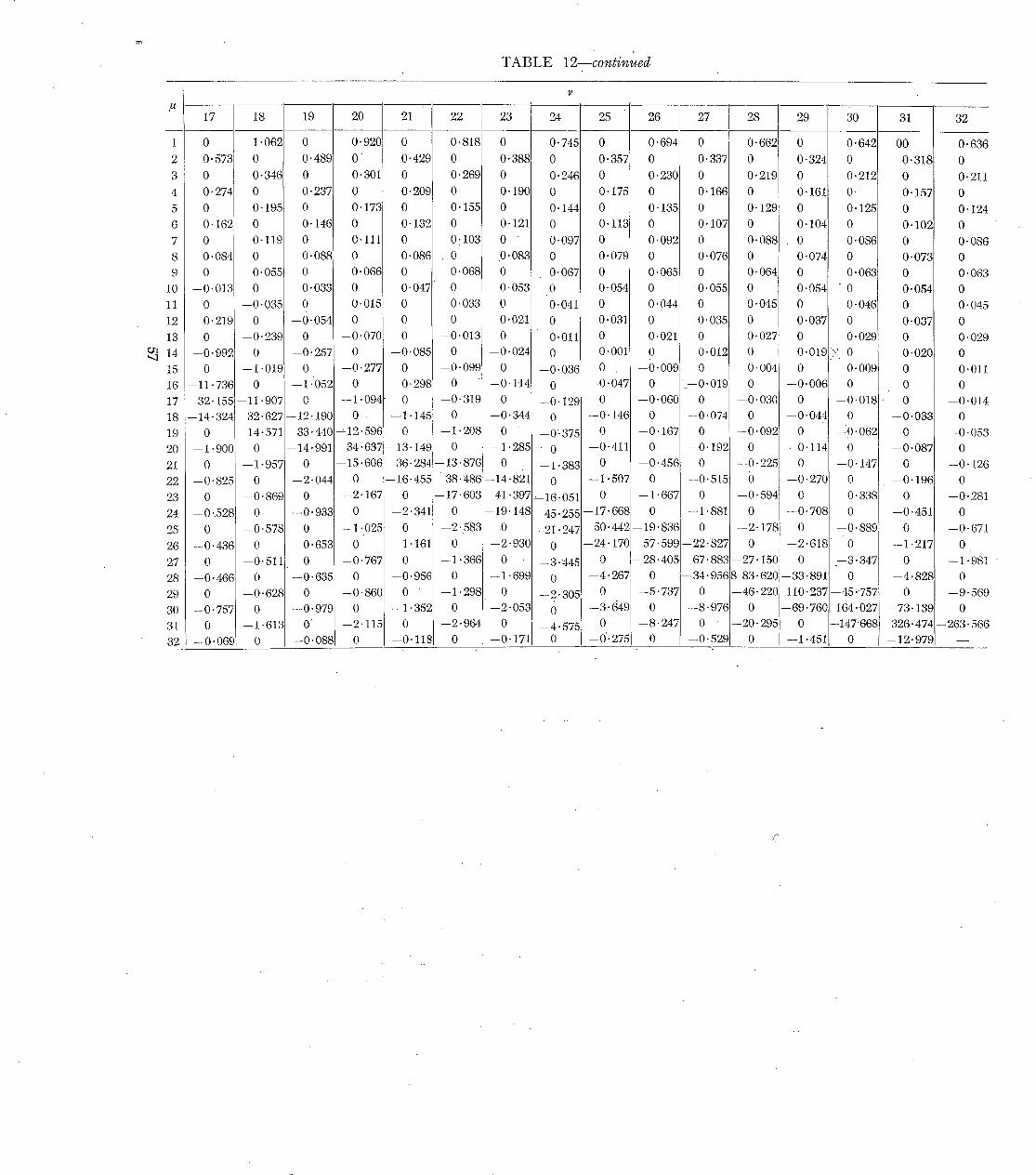
r r t

T A B L E 12--continued

¢.xt

#

1

2

3

4

5

6

7

8

9

10

11

12

13

14

15

16

17

18

19

20

21

22

23

24

25

26

27

28

29

30

31

32

17 18 19 20 21 22 23 24 25

0 1.062 0 0.920

0.573 0 0.489 0

0 0.346 0 0.301

0.274 0 0.237 0

0 0-195 0 0.173

0.162 0 0.146 0

0 0-119 0 0.111

0.084 0 0.088 0

0 0-055 0 0.066

--0.013 0 0.033 0

0 --0-035 0 0.015

--0.219 0 - -0 .054 0

0 --0.239 0 --0.070

--0.992 0 - -0 .257 0

0 --1.019 0 - -0 .277

--11-736 0 - -1 .052 0

32.155--11"907 0 ~1 .094

- -14 .324 32.627=-12.190 0

0

- -1 .900

0

--0.825

0

- -0 .528

0

- -0 .436

0

- - 0 - 4 6 6

0

--0.757

0

- -0 .069

0 0.818 0 0.745

0.429 0 0.388 0

0 0.269 0 0.246

0.209 0 0.190 0

0 0.155 0 0.144

0-132 0 0.121 0

0 0:103 0 0.097

0.086 0 9-083 0

0 0.068 0 0.067

0.047 0 0.053 0

0 0.033 0 0.041

0 0 0-021 0

0 --0.013 0 0.011

--0.085 0 --0.024 0

0 --0-099 0 --0-036

- 0 . 2 9 8 0 - -0 .1 t4 0

0 --0.319 0 --0.129

--1.145 0 --0.344 0

~--14-571 33"440~12"596 0 - -1 .208 0 __0:375

0 --14"991 34"637--13"149 0 - -1 .285 0

--1-9571 0 --15"606 36-284--13"876 0 --1"383

0 --2.044 0 --16-455 38"486--14-821 0

--0"869 0 --2"167 0 --17"603 41-397~16.051

0 --0-933 0 --2.341 0 --19.148

- -0 .578 0 --1.025 0 - -2t583 0

0 511 . - -0 .653 0 --1.161 0 --2-930 - -0 . 0 --0.767 0 - -1 .366 0

0 --0.635 0 --0.956 0 - -1 .699

- -0 .628 0 --0.860 0 - -1 .298 0

0 --0.979 0 - -1 .352 0 --2-053

--1 .613 O" --2.115 0 - -2 .964 0

0 --0"088 0 --0"118 0 --0.171

0

0.357

0

0.175

0

0.113

0

O. 079

0

0.054

0

O- 031

0

O. 001

0

- 0 . 0 4 7

0

--0.146

0

--0.411

0

--1.507

0

45.255--17"

--21.247 50. 0 --24.

--3.445 0 0 --4.267

--2.305 0 0 -3.649

--~.575 0 --0".275

26 27 28 29 30

0.694 0 0 • 662! 0 0"642

0 0.337 0 0-324 0

0.230 0 0-219 0 0.212

0 0.166 0 0.161 O.

0-135 0 0.129 0 0.125i

0 0.107 0 0-104 0

0.092 0 0-088 0 O.08E

0 0.076 0 0.074 0

0.065 0 0-064 0 0.063

0 0.055 0 0 . 0 5 4 - 0

0'044 0 0-045 0 0.046

0 0 . 0 3 5 0 0.037 0

0"021 0 0"027 0 0"029

0 0.012 0 0.019 }: 0

- -0 .009 0 0.004 0 0-009

0 - - 0 - 0 1 9 0 - -0 .006 0

--0.060 0 --0.030 0 --0.018-

0 --0-074 0 --0.044 0

--0.167 0 --0.092 0 --0.062

0 --0.192 0 --0.114 0

--0.456 0 --0-225 0 --0.147

0 --0.515 0 - -0 .270 0

--1.667 0 --0-594 0 - -0 .338

668 0 --1.881 0 --0-708 0

442--19.836 0 - -2 .178 0 - -0 .889

170 57.599--22.827 0 - -2 .618 0

--28.405 67.883--27.150 0 - -3 .347

0 - -34 .9568 83.620--33-891 0

--5-737 0 - 46.220 110-237--45.-757

0 - -8 .976 0 --69.760 164.027

--8.247 0 - 20-295 0 --147"668

0 - -0 .529 0 --1.451 0

31 32

O0 O. 636

0.318 0

0 0-211

O- 157 0

0 O. 124

O- 102 0

0 O- 08(

O. 073 0

0 0.062

O- 054 0

0 0-045

O- 037 0 0 O. 02 c

0.020 0

0 0.011

0 0

0 --0-014

--0-033 0

0 --0.05~

- - O- 087 0

0 --0.12~

--0- 196 0

0 --0- 281

- -0 . ;151 0

0 - -0- 671

--1 .217 0

0 -- 1. 981

- -4 . 828 0

0 --9.56c~

--73. 139 0

326- 474 --263- 56(

-- 12.979

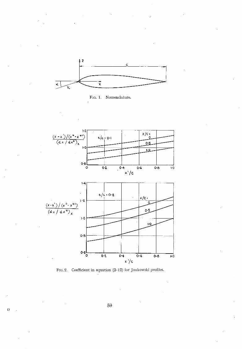
FIG. l . Nomenclature.

C× - ~ ') ICx *- x "') (~ / ~x~)~

1.0

0"~

t /C -- 0"4

/

/ /

X/C= 0 .....

/

0"5.._~ /

/

/

/

f

O 0-Z 0"4 0,~ 0.B I.~

(x-×') / Cx :"- x ~')

FIG. 2.

~'4

t.0

0.B

0.61

~/!' o.z

J f l J

/

_f f

x/c.

I ' 0 1 /

/ f

0 0,~. 0,4 0 . ~ 0 ,6 1.0

x '/C

Coefficient in equat ion (2-12) for Joukowski profiles.

59 El

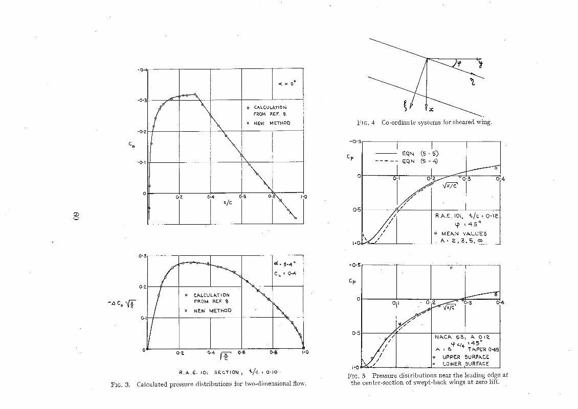
Ob 0

CI=

FIG. 3.

-04

-0.~

-0,1

K = 0

O,Z 0.4 ,/c

e C&LCU LfkTI0 N FROM REF. 9.

x NEW METHOD

O- 6 0 . ~

0"5

0-Z

Oq

® CALCULATION FROM ~EF. 9

x NEW METHOD

d,. 5.4. °

CL= 0.4-

O"& ~,.4 ~ 0'6 0"8 1.0

R.A.E. IO1 5EC..TION ~, "t-/c : O-Io '

Calculated pressure dis t r ibut ions for two-dimensional flow.

FIG. 4 Co-ordinate systems for sheared wing.

-0 '5

EQN Cs -Is) ] Cp . . . . . EQN (5 - 4) J

• ~ O G 0 2 ~ _ ~'0.$ 0

/ - # T ~

0"5 / I / R.A.E.,Oi, L / c=O. IP_ . , . { ) =4"5"

J , , / / ® ME/NN VA.L',JE,5 i.O~JC z A : ~_ ,~ ,5 co

f -_45 °

A -- 6 TfkPER 0"4.5 e UPPE.R 5URFACF..

I-0 ~'}"~"/ ~ LOWER SURFACE

FIO. 5 Pressure d is t r ibut ions near the leading edge at the centre-sect ion of swept-back wings at zero lift.

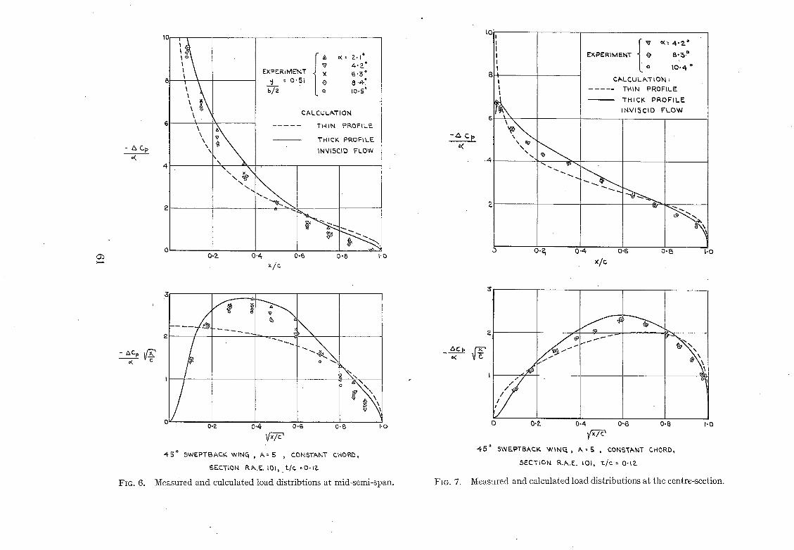
- &CI~

4

\ \ \ \ \ \

4.Z ° Ex~am~T . X e.~ °

"J : ° 5 ~ <~ 8.,~' . b / a e Io.S °

C AL C~JL~kTION

THIN PP~OFIL. E

THICK pROF~LK INVISC~O FLOW

0 . ~ 0"4 0-6 0 " 8 t . ~

×/c

- A , c.p

10

EX, P~'RIM ENT O e,-~ P

I o l O , 4 °

I I CF, LCUL ~,T 10N : THIN PROFILE I

~ ~ THICK PROFII.~. INVISCID FLOW

~'~ ~ ~

0 0 . ~ 0-4 o.6 o - g

x / c I-0

- ACp

FIG. 6.

\

o.?. 0.4 0.6 o.8 ~-o

4"5 0 5WSPTBAC~. WINCq , A = 5 3 CONSTANT CHORD,

~ECTtQN R./k.E. 10I, t /P, ,O.l~

Measured and culculated load distribtions at mid-semi-span.

a

t

FIG. 7.

/ / /

45 = 5WEI=q-BACK WIN~ , A,,S , CONS"[~,NT CHORD,

SECTION R./K.E. IOI, t / c : o-i~_

Measured and calculated load distributions at the centre-section.

0 O'Z 0.4 0"6 O.B Po

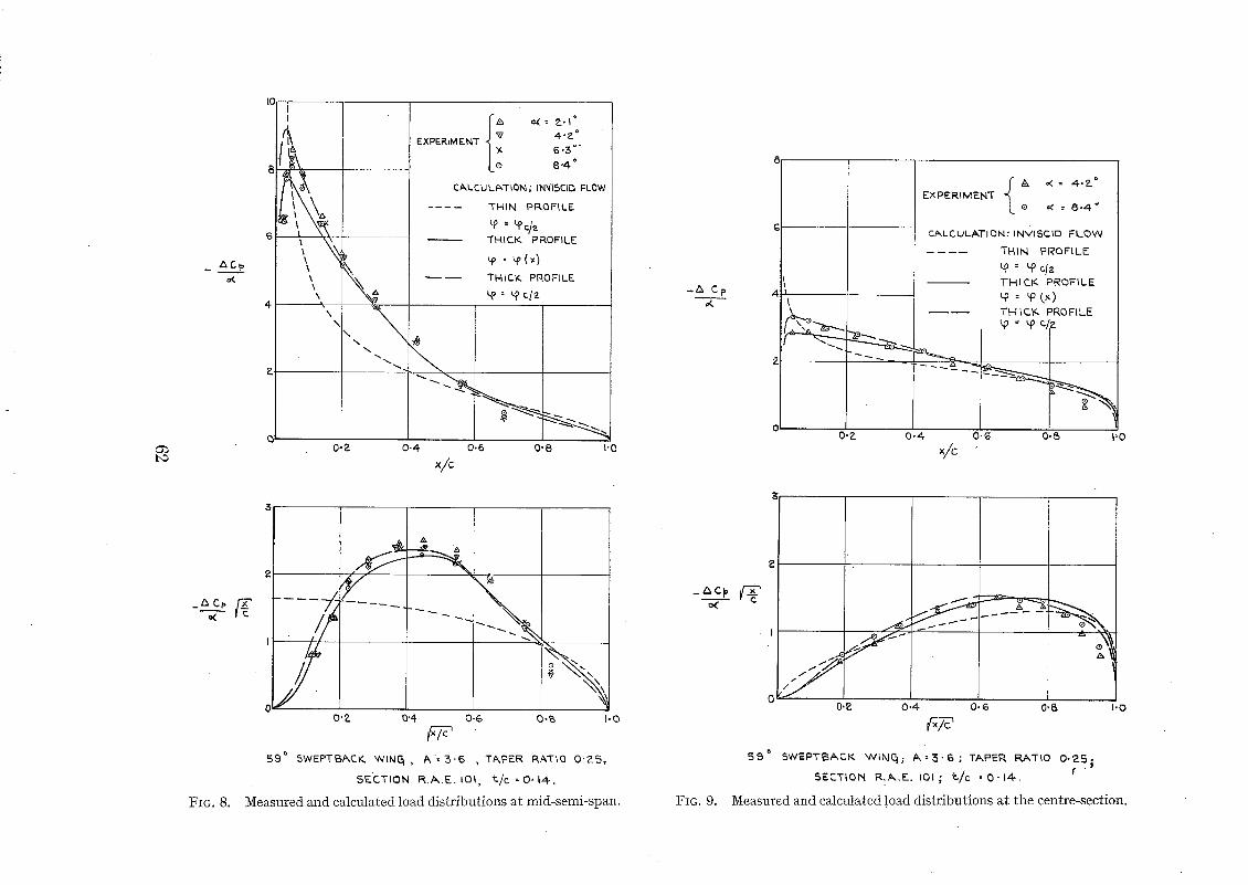
G~

- A C p

K

FIG. 8.

Ic i

4

I

\ \ \ \ \ \

0-2

--- ... - - . ~

0 - 4

f ! o( = t . I ° EXPERIM E.NT 4" ~. {' B 4 o"

e.4 °

CkLCULATION ; INVISCII~ FLOW

THIN PROFILE

~P = %]a THICK PROFILE

THICK PROFILE

: '-p cla

0 . 6 0 - 8 I-0

/ #

0

, x

04_ O'4 0.6 0 4 , I -0

59 ° 6WEPTBACK WIN~ , A : 3 . 6 , T~,PER RATIO 0 " 2 5 ,

5ECTION R . A . E . IOI t / c = 0 . 1 4 .

Measured and calculated load d i s t r i bu t ions at mid-semi-span.

_A Cp

FIG. 9.

EXPERIMENI" ~ A K = 4 .2 . "

L o ~ =8.4 °

('-ALC.ULATION: INVlSCII3 FLOW

THIN PROFILE

TII ICK. PROFILE ~p = ~p (,x)

TN I Cic. PROFILE

0.~ 0-~ I '0

o<

/ -j 0.g 0.4 0.6 0"& t.O

5 9 a SWEPTBACK W t N ~ ; A ° ~ . c o ; TAPER RATIO 0,9_5~

SECTIOM R.~,.E, 10i; ~,/c * 0 . 1 ~ . ¢ "

Measured and calculated ]oad d i s t nbu t l ons a t the centre-sect ion.

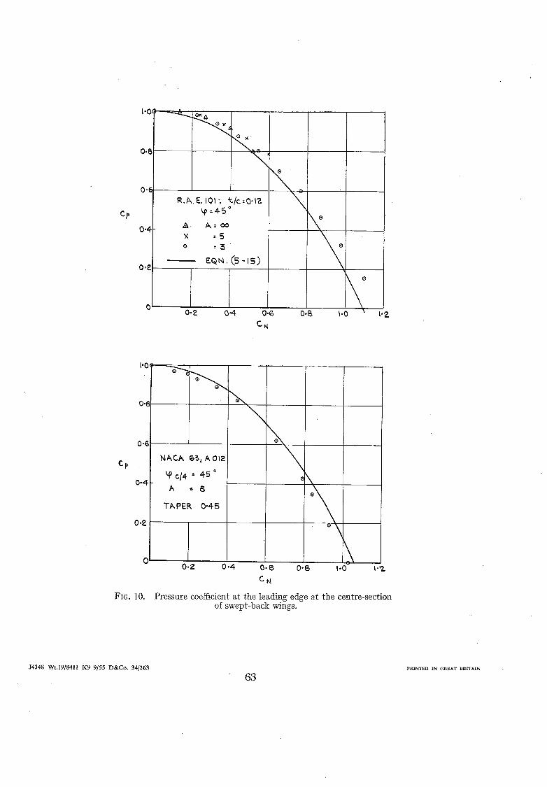
Cp

0.B

0 , 2

R.A.E. I01 ; *-/c:0.~?- q~-- 4.5"

& • : o o X : 5 o - - 5

e Q N ( s - t s )

0.~ 0-4

\ 0 \

0.6 Cu

O-B ~.0 ~.'2.

I'O

N/~CA @~j A 012 Cp ~o c/4 ~ 4 s *

0.4- A * 8

TAPER, 0.4.S

0.~.

FIG. 10.

\ 0-2 0 .4 0 . 6 0"~ 1.0 I"9_

CN

Pressure coefficient at the leading edge at the centre-section of swept-back wings.

J4348 Wt.19/8411 K9 9[55 D&Co. 34•263

63 PRINTED IN GREAT BRITAIN

R. & M . N o . 2 9 1 8

'r.

Publications of the Aeronautical Research Council

ANNUAL TECHNICAL REPORTS OF THE AERONAUTICAL RESEARCH COUNCIL (BOUND VOLUMES)

1938 Vol. I. Aerodynamics General, Performance, Airscrews. 5os. (5IS. 8d.) Vol. II. Stability and Control, Flutter, Structures, Seaplanes, Wind Tunnels, Materials. 3os. (31s. 8d.)

1939 Vol. I. Aerodynamics General, Performance, Airscrews, Engines. Sos. (5IS. 8d.) Vol. n . Stability and Control, Flut ter and Vibration, Instruments, Structures, Seaplanes, etc.

63 s. (64 s. 8d.)

194o Aero and Hydrodynamics, Aerofoils, Airscrews, Engines, Flutter, Icing, Stability and Control, Structures, and a miscellaneous section. 5os. (5IS. 8d.)

1941 Aero and Hydrodynamics, Aerofoils, Airscrews, Engines, Flutter, Stability and Control, Structures. 63 s. (64 s. 8d.)

1942 Vol. I. Aero and Hydrodynamics, Aerofoils, Airscrews, Engines. 75 s. (76s. 8d.) Vol. II. Noise, Parachutes, Stability and Control, Structures, Vibration, Wind Tunnels. 47 s. 6d.

(49 s. "2d.) "

1943 Vol. I. Aerodynamics, Aerofoils, Airscrews. 8os. (8is. 8d.) Vol. n . Engines, Flutter, Materials, Parachutes, Performance, Stability and Control, Structures.

9os. (9IS. iid.)

x944 Vol. I. Aero and Hydrodynamics, Aerofoils, Aircraft, Airscrews, Controls. 84 s. (86s. 9d.) Vol. II. Flutter and Vibration, Materials, Miscellaneous, Navigation, Parachutes, Performance,

Plates and Panels, Stability, Structures, Test Equipment, Wind Tunnels. 84 s. (86s. 9d.)

ANNUAL REPORTS OF THE AERONAUTICAL RESEARCH COUNCIL-- 1933-34 is. 6d. (is. 8½d.) 1937 2s. (2s. 2½d.) 1934-35 " is. 6d. (is. 8½d.) 1938 is. 6d. (is. 8~d.)

April I, 1935 to Dec. 31, 1936 4 s. (4 s. 5½d.) 1939-48 3 s. (3 s. 3½d.)

INDEX TO ALL REPORTS AND MEMORANDA PUBLISHED IN THE ANNUAL TECHNICAL REPORTS, AND SEPARATELY--

April, I95o . . . . . R. & M. No. 26o0. 2s. 6d. (2s. 7½d.)

AUTHOR INDEX TO ALL REPORTS AND MEMORANDA OF THE AERONAUTICAL RESEARCH COUNCIL--

I9O9-January, 1954 - - - R. & M. No. 2570. I5 s. (I5 s. 5½d.)

INDEXES TO THE TECHNICAL REPORTS OF THE AERONAUTICAL RESEARCHCOUNCIL,--

December I, 1 9 3 6 - June 3o, 1939. R. & M. No. 185o. July I, 1939 - - June 3o, 1945. - R. & M. No. 195o. July I, 1945 - - June 3 o, 1946. - R. & M. No. 2050. July I, 1946 - - December 31, 1946. R. & M. No. 215o. January i, 1947 June 3o, 1947. - R. & M. No. 2250.

PUBLISHED REPORTS AND MEMORANDA "0F THE AERONAUTICAL

Between Nos. 2251-2349. - - R . & M. NO. 2350. Between Nos. 2351-2449. - - R. • M. No. 2450. Between Nos. 2451-2549. - - R. & M. No. 255o. Between Nos. 2551-2649. - - R. & M. No. 265o.

Pyices in brackets include ~ostage

H E R MAJESTY'S S T A T I O N E R Y O F F I C E York House, Kingsway, London W.C.2; 423 Oxford Street, London W.1 (Post Orders: P.O. Box 569, London S.E.1); 13a Castle Street, Edinburgh 2; 39 King Street, Manchester 2; 2 Edmund Street, Birmingham 3; 109 St. Mary Street,

Cardiff; Tower Lane, Bristol 1; 80 Chiehester Street, Belfast, or through any bookseller f

~s. 3d. (is. 4½d.) is. (is. z½d.) l~.(xs, x½d.) IS. 3 d. (IS. 4½/¢.) IS. 3 d . (IS. 4½d.)

RESEARCH C O U N C ~ - -

IS. 9d. (IS. Io½d.) 2 s . (2s. i½d.) Zs. 6d. (2s. 7½d.) /,

2s. 6d. (2s. 7½d.)

$.O. Code No. 23-2918

R. & M . N o . 2918