MIT OpenCourseWare http://ocw.mit.edu

2.672 Project Laboratory Spring 2009

For information about citing these materials or our Terms of Use, visit: http://ocw.mit.edu/terms.

MASSACHUSETTS INSTITUTE OF TECHNOLOGY

DEPARTMENT OF MECHANICAL ENGINEERING

2.672 PROJECTS LABORATORY

LABORATORY MANUAL

Spring Term2009

This Page Intentionally Left Blank

1

___________________________________________________________________________

____________________________________________________________________________

____________________________________________________________________________

2.672 Spring, 2009 SCHEDULE

MONDAY PM SECTION 13:00-16:00 ADD DATE 3/6 - DROP DATE 4/23

1st Lab 2/9, 2/17, 2/23, 3/2 1st lab report due 3/9 2nd Lab 3/9, 3/16, 3/30, 4/6 2nd lab report due 4/13 3rd Lab 4/13, 4/27, 5/4 (3 Sessions Only) Oral Presentation 5/11, Class Time Note: Class on Tuesday 2/17, No class on 3/23 (Spring Break) or 4/20 (Patriots Day)

TUESDAY PM SECTION 14:00-17:00 ADD DATE 3/6 - DROP DATE 4/23

1st Lab 2/3, 2/10, 2/24, 3/3 1st lab report due 3/10 2nd Lab 3/10, 3/17, 3/31, 4/7 2nd lab report due 4/14 3rd Lab 4/14, 4/28, 5/5 (3 Sessions Only) Oral Presentation 5/12, Class Time Note: No class on 2/17 (Presidents Day), 3/24 (Spring Break), or 4/21 (Patriots Day)

FRIDAY PM SECTION 14:00-17:00 ADD DATE 3/6 - DROP DATE 4/23

1st Lab 2/6, 2/13, 2/20, 2/27 1st lab report due 3/6 2nd Lab 3/6, 3/13, 3/20, 4/3 2nd lab report due 4/10 3rd Lab 4/10, 4/17, 4/24 (3 Sessions Only) Oral Presentation 5/1, Class Time Note: No class on 3/27 (Spring Break) or 5/8 (Schedule Balance)

2

2.672 - Staff

Instructors in Charge: Professor Wai Cheng Extension

Professor Douglas Hart Extension

Instructors: Dr. Barbara Hughey Extension

Prof. Richard Kimball

Mr. Bryan Ruddy Extension

Sections Monday P.M. Section

Mr. Bryan Ruddy

Tuesday P.M. Section

Prof. Douglas Hart

Friday P.M. Section

Prof. Richard Kimball

3

CONTENTS

PAGECOURSE SCHEDULE 2

INSTRUCTOR AND STAFF INFORMATION 3

CONTENTS 4

SECTION 1. COURSE OUTLINE AND GRADING POLICY 5

SECTION 2. DESCRIPTION OF EXPERIMENTS 7

1. Proximity Heating of Silicon Wafers 8

2. Transfer Line Dynamics 9

3. Heat Exchanger Tube Vibrations 10

4. Pipe Clearing Fluid Transient 11

5. Irradiation Sample Transfer Line Snubbing Section Behavior 12

6. Peak Pressure in Nuclear Containment Vessel 13

7. Irrigation System Pressure Surge 14

SECTION 3. GUIDE TO 2.672 REPORT WRITING 15

SECTION 4. GUIDE TO 2.672 ORAL PRESENTATIONS 19

SECTION 5. SOFTWARE FOR 2.672 21

Matlab 22Importing data files from the data acquisition system 24Plotting 24To import graphs into Microsoft Word Document 25Script files 25Integration of ordinary differential equations 26List of Matlab programs for 2.672 projects 29

4

SECTION 1: 2.672 COURSE OUTLINE AND GRADING POLICY

2.672 Project Laboratory

PURPOSE: This course will provide experience in formulating, solving, and presenting solutions to engineering problems.

ORGANIZATION: Groups of two or three students will work together on three experiments. During the assigned time, a faculty member will be available in the laboratory and will assist with problems which arise. Since a significant purpose of the course is to allow you to learn problem solving techniques, the lab instructors will provide guidance, but will not, in general, tell you what to do.

RULES: Students are to be in the laboratory only at assigned times, unless by special permission. Attendance for the entire scheduled 3-hour laboratory session is mandatory – absence will be reflected

in your final grade. Written reports are to be written independently - while all of the reports in a group should be based on

the same data, their text and figures must be created individually. Use of materials from course "bibles" or lab reports from previous terms or other groups is

strictly prohibited.

Written reports are due electronically on the class web site before the start of class on the due date. Each student may use up to a total of 48 hours of "grace" time for late reports without penalty; i.e. one

report may be 48 hours late and the other on time, both reports may be 24 hours late, or anywhere in between. Reports turned in later than the grace time allows will be penalized at the discretion of the instructor.

WRITTEN REPORTS: It is anticipated that all written reports in a group will have data, calculations and figures which are similar, but will have separately written texts. If for any reason some figures, tables, appendices or other material are copied and shared among the group, such materials should be initialed by the person who prepared the original. We want each of you to have the experience that accompanies writing a report but do not expect you to have different experimental results when you've run the same experiment. In general, each report should have enough detail so that the reader can reproduce your results. (See Section 3: Guide to 2.672 Report Writing.) In the last week of the first experiment, one hour will be spent in a brief workshop on report writing.

ORAL REPORTS: The results from your final experiment will be presented in an oral presentation by your group collectively. Oral presentations are an important part of communicating your results, so it should be a valuable experience. (See Section 4: Guide to 2.672 Oral Presentations.)

5

Grading Policy for 2.672

There will be 3 experiments. An independently written report by each student is required for the first two; an oral presentation by the group as a whole is required for the third experiment.

A letter grade (with pluses and minuses) will be given to each report. The final grade, however, is computed by assigning a number to each letter grade, and the following weighting is used.

1st report (written) 25% 2nd report (written) 25% 3rd report (Oral) 25% Lab performance (participation, knowledge of the subject etc.) 25%

To encourage using the laboratory as learning environment, substantial weighting is assigned to the lab performance which is subjectively graded. It should be noted that much of this grade is based on the

communication between you and your instructor in class. You should use the interaction to demonstrate your knowledge of the subject matter.

Late reports will be down graded. The downgrading is progressive as a function of the days past due. The grade discount is at the discretion of the instructor who will be grading the reports.

For the first two written reports, the grading will be based half on technical content and half on how well do you communicate in writing.

6

SECTION 2: 2.672 EXPERIMENTS

7

1. Proximity Heating Of Silicon Wafer

Lithography is a critical processing step in fabrication of advanced microcircuits. It transfers a circuitry layout from a photomask to a silicon wafer. A layer of photosensitive polymers (photoresist) is first spin-coated onto the silicon substrate. A lithography system then projects the image of the photomask onto the resist coating and creates a latent image in the resist. The photoresist in the exposed (or un-exposed) area is then removed by chemical etching

The latent image needs to be activated before the etching process. This is accomplished by setting the wafer temperature to around 180 C for a few seconds; etching quality control requires the temperature to be uniform to within 2 C over the entire wafer surface. A hot-plate heating technology is currently used. The wafer is first supported at ~2.5 cm away from the hot-plate surface. The wafer is then released and lowered quickly to a close proximity (of preset distance) of the hot plate. After a certain amount of heating time, the wafer is lifted away from the hot plate, picked up by a robot and then placed on a chilled plate to cool down.

It is important to reduce the wafer heating time in order to increase process throughput: the thermal activation time for the photo-resist only requires a few seconds at 180o C. You are hired as a consultant by a semiconductor equipment company to identify parameters that will affect the wafer heating rate, to establish a model that can accurately predict the transient wafer temperature, and to propose techniques to reduce the heating time and thus increase process throughput.

Specific questions to be addressed are:

a) Are the steady state temperature differences between the hot plate and the wafer as a function of the gap size consistent with the theoretical model of the heat transfer processes?

b) What does the heat-up time (either (1-1/e) or 10-90% rise time) depend on? Is your theory consistent with the measurement?

c) The smaller the gap, the faster is the heat up time. What determines the lower limit of the gap size?

Experiment

A simplified hot-plate heating experiment has been set up in the lab. A typical test run includes the following steps:

1. Place small pieces of paper around the edge of the hot plate as spacers for setting the gap between the hot plate and the wafer. When you measure the thickness of the paper, do not squeeze it too much, since the wafer is not very heavy.

2. Lower the test wafer onto the hot plate. The distance between the wafer and hot plate is determined by the paper thickness.

3. Measure the plate temperature and the transient wafer temperature. Because of the low level signal (type K thermocouple response is 40 V/oC), the amplified signal is noisy. You may filter the signal by using the Matlab filters (the functions are “butter” for the Butterworth filter design, and “filtfilt” for the phase preserving filtering; use the help function to find out the usage).

4. Cool the wafer by lifting the wafer away from the hot plate after the wafer temperature has reached a steady-state value. There is an air jet set up in the lab to cool the wafer.

The hot-plate temperature should be set between 120 C and 150 C. (The paper spacer will char if the temperature is too high. When the temperature is too low, the thermocouple signal is buried in the noise.) You should investigate experimentally the significant effect of wafer-plate distance on the wafer heating rate.

(Note: the thermal properties of silicon may be found on the web. The wafer is not doped, so the emissivity is low – is of the order of 0.01 to 0.05.)

8

2. Transfer Line Dynamics

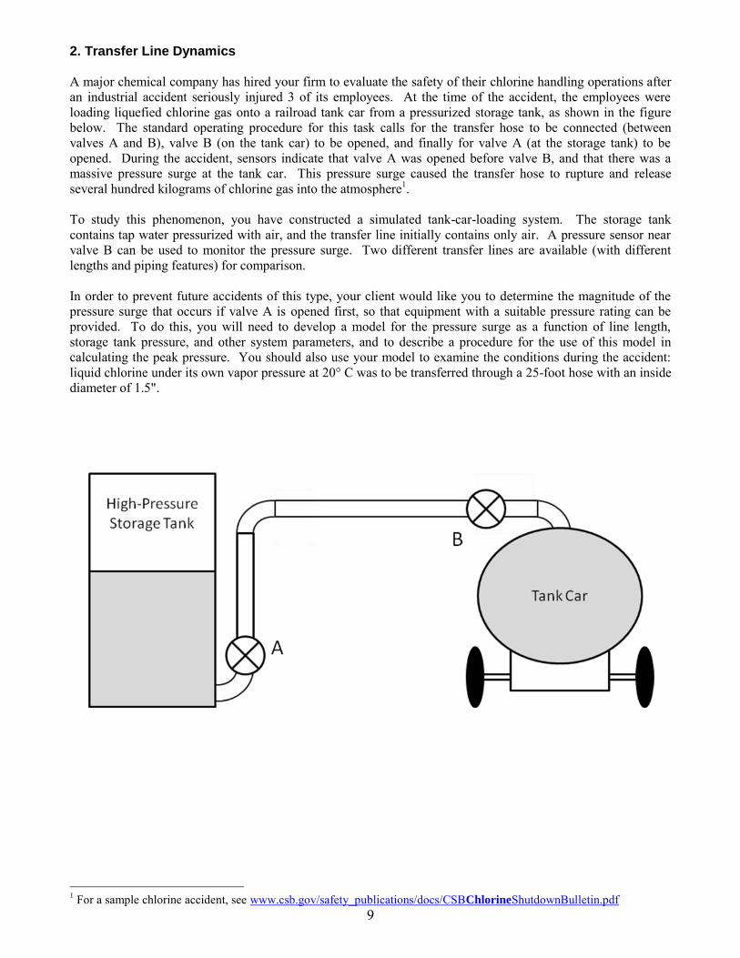
A major chemical company has hired your firm to evaluate the safety of their chlorine handling operations after an industrial accident seriously injured 3 of its employees. At the time of the accident, the employees were loading liquefied chlorine gas onto a railroad tank car from a pressurized storage tank, as shown in the figure below. The standard operating procedure for this task calls for the transfer hose to be connected (between valves A and B), valve B (on the tank car) to be opened, and finally for valve A (at the storage tank) to be opened. During the accident, sensors indicate that valve A was opened before valve B, and that there was a massive pressure surge at the tank car. This pressure surge caused the transfer hose to rupture and release several hundred kilograms of chlorine gas into the atmosphere1.

To study this phenomenon, you have constructed a simulated tank-car-loading system. The storage tank contains tap water pressurized with air, and the transfer line initially contains only air. A pressure sensor near valve B can be used to monitor the pressure surge. Two different transfer lines are available (with different lengths and piping features) for comparison.

In order to prevent future accidents of this type, your client would like you to determine the magnitude of the pressure surge that occurs if valve A is opened first, so that equipment with a suitable pressure rating can be provided. To do this, you will need to develop a model for the pressure surge as a function of line length, storage tank pressure, and other system parameters, and to describe a procedure for the use of this model in calculating the peak pressure. You should also use your model to examine the conditions during the accident: liquid chlorine under its own vapor pressure at 20° C was to be transferred through a 25-foot hose with an inside diameter of 1.5".

1 For a sample chlorine accident, see www.csb.gov/safety_publications/docs/CSBChlorineShutdownBulletin.pdf 9

3. Heat Exchanger Tube Vibrations

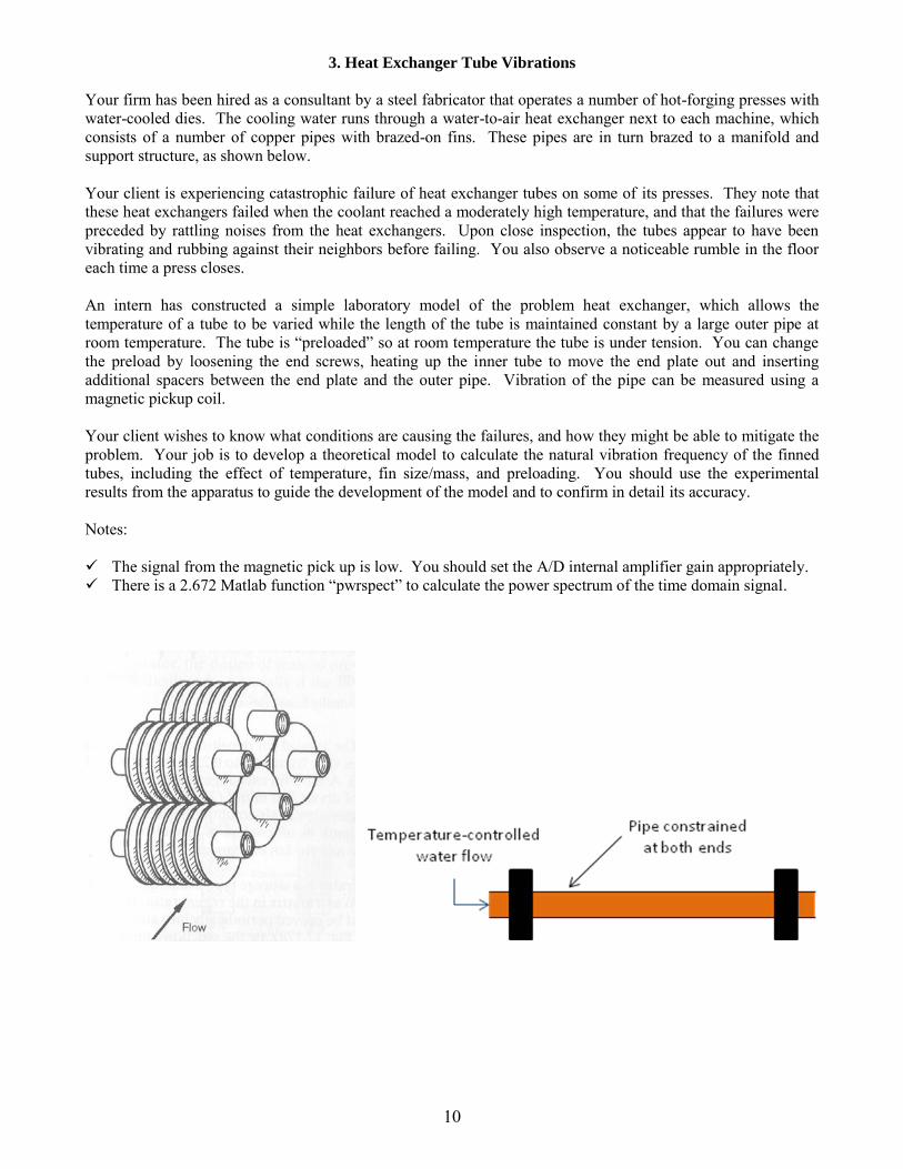
Your firm has been hired as a consultant by a steel fabricator that operates a number of hot-forging presses with water-cooled dies. The cooling water runs through a water-to-air heat exchanger next to each machine, which consists of a number of copper pipes with brazed-on fins. These pipes are in turn brazed to a manifold and support structure, as shown below.

Your client is experiencing catastrophic failure of heat exchanger tubes on some of its presses. They note that these heat exchangers failed when the coolant reached a moderately high temperature, and that the failures were preceded by rattling noises from the heat exchangers. Upon close inspection, the tubes appear to have been vibrating and rubbing against their neighbors before failing. You also observe a noticeable rumble in the floor each time a press closes.

An intern has constructed a simple laboratory model of the problem heat exchanger, which allows the temperature of a tube to be varied while the length of the tube is maintained constant by a large outer pipe at room temperature. The tube is “preloaded” so at room temperature the tube is under tension. You can change the preload by loosening the end screws, heating up the inner tube to move the end plate out and inserting additional spacers between the end plate and the outer pipe. Vibration of the pipe can be measured using a magnetic pickup coil.

Your client wishes to know what conditions are causing the failures, and how they might be able to mitigate the problem. Your job is to develop a theoretical model to calculate the natural vibration frequency of the finned tubes, including the effect of temperature, fin size/mass, and preloading. You should use the experimental results from the apparatus to guide the development of the model and to confirm in detail its accuracy.

Notes:

The signal from the magnetic pick up is low. You should set the A/D internal amplifier gain appropriately. There is a 2.672 Matlab function “pwrspect” to calculate the power spectrum of the time domain signal.

10

4. Pipe Clearing Fluid Transients

Your firm has been hired by an apple orchard in rural Massachusetts to design its new cider pasteurization equipment. This orchard only makes cider during a short period in the fall; the equipment is stored in an unheated barn during the rest of the year. For sanitary reasons, the equipment is to be flushed with water at the end of the season. To prevent freezing damage during the winter, and to keep the equipment clean for the remainder of the year, it has been proposed that the pipes in the pasteurizer be blown dry with filtered shop air before storage.

The project lead is concerned that this air purge procedure may result in damage to the pasteurizer as slugs of residual water are forced around the numerous tubing bends2. You have been tasked with modeling the forces exerted by these water slugs as they are cleared by high-pressure air. Your model will be used by the design team to choose orifices that will restrict the purge flow, and thus transient pipe forces, to safe levels.

A member of the design team has made a bench-level experimental model of the pasteurizer, consisting of a section of plastic pipe in which a measurable amount of water can be trapped. This water is driven out of the pipe by an air flow metered by a choked flow orifice of known diameter, which is that of the throat area of the solenoid valve used to switch on the flow. The nominal orifice size is stated on the valve body. Due to the compact valve design, the valve's discharge coefficient is significantly lower than 1. (If you have time, you can calibrate the discharge coefficient by discharging the tank; if you do not, you can assume a discharge coefficient of 0.5.) The mass flow rate through this orifice can then be calculated using formulas that are in your fluid mechanics text books under the section of compressible flow. The pressure exerted by the slug of moving water is recorded by a pressure transducer on the pipe elbow. From this pressure, the force on the elbow may be deduced.

Air tank

pipe

water

solenoid valve

Pressure transducer

Air tank

pipe

water

solenoid valve

Pressure transducer

2 For instance, see http://www.dairyengineering.com/juicepasteur.asp 11

5. Irradiation Sample Transfer Line Snubbing Section Behavior

The M.I.T. reactor is used to irradiate various isotope samples so that they can be used for medical treatment and research. These samples are packaged in a small cylinder and then inserted into a curved transfer line and lowered to the core of the reactor. (The curved line is to prevent personnel from radiation exposure at the point of insertion.) The sample is retrieved after a suitable interval. If the retrieval system fails, the sample drops to the bottom. To prevent such an accident from damaging the transfer line or the materials in the cylinder, a snug-fitting sleeve section has been installed in the bottom of the transfer line. The clearance between the cylinder and the tube in this section is small enough that air is trapped below the cylinder and is released slowly; this results in reduction in the speed of the cylinder.

This investigation has been commissioned to develop a methodology for designing the snubbing section. To verify the methodology, the experimental values of interest are:

a) The cylinder impact velocity at the bottom of the transfer line, as a function of the cylinder mass.

b) An estimate of the distance the cylinder has traveled before it bounces back as a function of the cylinder mass. (How would you estimate it from the data?)

c) The pressure of the air trapped in the line, both the peak value and the value when the cylinder has reached terminal velocity.

Note that results (a) and (b) are important to verify that your line design model is correct; (c) is just data for checking your theory. (The pressure is negligible compared to the materials yield strength.)

In the actual case, the air at the bottom of the tube is not at room temperature, but at a temperature of about 300oC. Also, the actual drop is one meter taller than the one in the lab. Thus, after confirming the validity of the model with the lab apparatus, the model must be used to predict results for the actual situation.

A simulated transfer line has been set up in the lab. The velocity of the cylinder before entering the snubbing section can be measured by determining the transit time of the cylinder as it passes a light sensor. Similarly, the velocity at impact may be obtained from the light sensor signal at the bottom of the tube. The pressure versus time behavior can be measured with the pressure transducer installed in the snubbing section. The mass of the cylinder can be altered by unscrewing the top and changing the mass of pellets inside.

A model for the motion of the sample in the snubbing section should be developed compared to the experiment. You have to formulate and solve the set of differential equations describing the dynamics of the system. (The terminal velocity is the steady state solution.) You may use MATLAB or write a simple program to simulate the dynamic behavior.

The critical questions to be answered with the model are:

(i) What is the impact velocity? (ii) How long should the snubbing section be?

To answer (ii), you have to get your model to reproduce the experimental results (especially item (b) in the above) with reasonable confidence. Then the model is applied to snubbing sections of different lengths to see whether the cylinder reaches the terminal velocity before hitting the bottom.

12

Simulated

containment

vessel

Simulated reactor

Top break

Bottom break

Saturated water

Saturated steam

Simulated

containment

vessel

Simulated reactor

Top break

Bottom break

Saturated water

Saturated steam

6. Peak Pressure in Nuclear Containment Vessel

Every nuclear reactor is surrounded by a containment vessel designed to prevent the release of radioactive products if there is a catastrophic break in the reactor pressure vessel. The containment vessel must be strong enough to contain the steam and water released but must not be grossly over designed since it is a major element in the overall cost of the power plant. The purpose of this investigation is to develop and confirm a method of calculating the peak pressure in such a containment vessel after a sudden release of liquid and vapor into it.

The experimental apparatus consists of a small tank simulating the reactor and a larger tank simulating the containment structure. The reactor tank can be filled with liquid water and pressurized with steam; ~20% to 70% liquid by volume is appropriate. The water in the reactor vessel can be discharged into the containment vessel by opening a valve at the bottom or the top, simulating a break at the steam side, or at the liquid side of the water in the reactor. (You should make sure that the liquid water and the steam in the reactor tank are equilibrated before the discharge.) The pressure versus time response in the containment vessel and several other temperatures and pressures can be measured routinely.

You should propose and verify a method of calculating the peak pressure in the vessel including, at least, the variation of the peak pressure with initial reactor pressure and liquid volume. The calculation will involve the solution of a set of nonlinear simultaneous equations by iteration. For your convenience, Matlab functions are available to determine the saturation properties of water as a function of pressure (or temperature). Using this function in a program you write, you could solve the set of equations for the peak pressure. See the Matlab write up for details of using the functions.

In your report, you should use your method to examine the peak pressure dependence on the various parameters, especially the ratio of the volumes of the containment and reactor vessels. Arrange your results intelligently so that they can be readily used in engineering design.

13

7. Irrigation System Pressure Surge

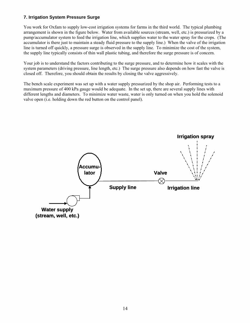
You work for Oxfam to supply low-cost irrigation systems for farms in the third world. The typical plumbing arrangement is shown in the figure below. Water from available sources (stream, well, etc.) is pressurized by a pump/accumulator system to feed the irrigation line, which supplies water to the water spray for the crops. (The accumulator is there just to maintain a steady fluid pressure to the supply line.) When the valve of the irrigation line is turned off quickly, a pressure surge is observed in the supply line. To minimize the cost of the system, the supply line typically consists of thin wall plastic tubing, and therefore the surge pressure is of concern.

Your job is to understand the factors contributing to the surge pressure, and to determine how it scales with the system parameters (driving pressure, line length, etc.) The surge pressure also depends on how fast the valve is closed off. Therefore, you should obtain the results by closing the valve aggressively.

The bench scale experiment was set up with a water supply pressurized by the shop air. Performing tests to a maximum pressure of 400 kPa gauge would be adequate. In the set up, there are several supply lines with different lengths and diameters. To minimize water waste, water is only turned on when you hold the solenoid valve open (i.e. holding down the red button on the control panel).

Accumu-

lator

Irrigation spray

Supply line Irrigation line

Valve

Water supply

(stream, well, etc.)

Accumu-

lator

Irrigation spray

Supply line Irrigation line

Valve

Water supply

(stream, well, etc.)

14

SECTION 3: A GUIDE TO 2.672 LAB REPORT WRITING

ELEMENTS OF A LABORATORY REPORT

1. Title page

2. Abstract

3. Table of Contents*

4. List of Symbols*

5. Introduction

6. Theoretical Analysis

7. Apparatus and Procedure

8. Results and discussion

10. Conclusions (and Recommendations)

11. Appendices*

12. References

*Optional

Individual reporting

You can share ideas, data and results with your group members. You need, however, to write your own project report.

Focus on your contribution

You should focus on your contributions to the understanding and solution of your project problem. You developed a model to characterize the problem. It is a remarkable achievement. Although your model may not be perfect, it is an important tool to understand the essential physical processes. Write your report to help people understand and solve real-world engineering problems. Do not write the report focusing on how inaccurate your model is.

Writing style

In general, do not use “I” , “we”, “he”, or “she” in technical writing. Here are some examples.

Example 1. “This work developed an engineering model to assess wafer temperature in hot-plate photoresist processing.”

Example 2. “The experimental system consists of three major parts.”

Write directly, avoid words that are not useful; e.g. “in order to”, “the purpose of this experiment is to”, etc.

Number of significant digits

If you report a temperature of 100.002 C, it suggests that the temperature error is less than 0.001 C. You should present your results with the right number of significant digits to represent the accuracy of your experiments and model simulations.

15

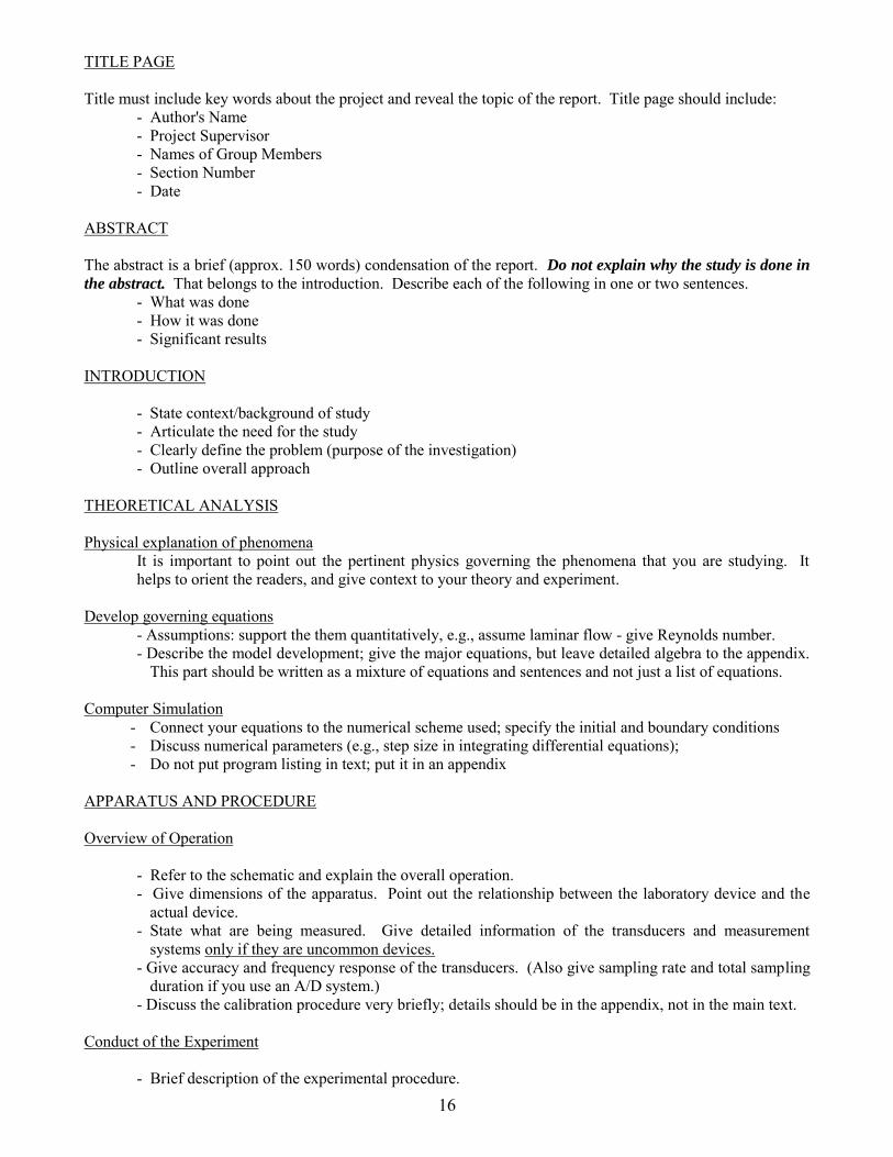
TITLE PAGE

Title must include key words about the project and reveal the topic of the report. Title page should include: - Author's Name - Project Supervisor - Names of Group Members - Section Number - Date

ABSTRACT

The abstract is a brief (approx. 150 words) condensation of the report. Do not explain why the study is done in

the abstract. That belongs to the introduction. Describe each of the following in one or two sentences. - What was done - How it was done - Significant results

INTRODUCTION

- State context/background of study- Articulate the need for the study- Clearly define the problem (purpose of the investigation)- Outline overall approach

THEORETICAL ANALYSIS

Physical explanation of phenomena It is important to point out the pertinent physics governing the phenomena that you are studying. It helps to orient the readers, and give context to your theory and experiment.

Develop governing equations - Assumptions: support the them quantitatively, e.g., assume laminar flow - give Reynolds number. - Describe the model development; give the major equations, but leave detailed algebra to the appendix.

This part should be written as a mixture of equations and sentences and not just a list of equations.

Computer Simulation - Connect your equations to the numerical scheme used; specify the initial and boundary conditions - Discuss numerical parameters (e.g., step size in integrating differential equations); - Do not put program listing in text; put it in an appendix

APPARATUS AND PROCEDURE

Overview of Operation

- Refer to the schematic and explain the overall operation. - Give dimensions of the apparatus. Point out the relationship between the laboratory device and the

actual device. - State what are being measured. Give detailed information of the transducers and measurement

systems only if they are uncommon devices. - Give accuracy and frequency response of the transducers. (Also give sampling rate and total sampling

duration if you use an A/D system.) - Discuss the calibration procedure very briefly; details should be in the appendix, not in the main text.

Conduct of the Experiment

- Brief description of the experimental procedure.

16

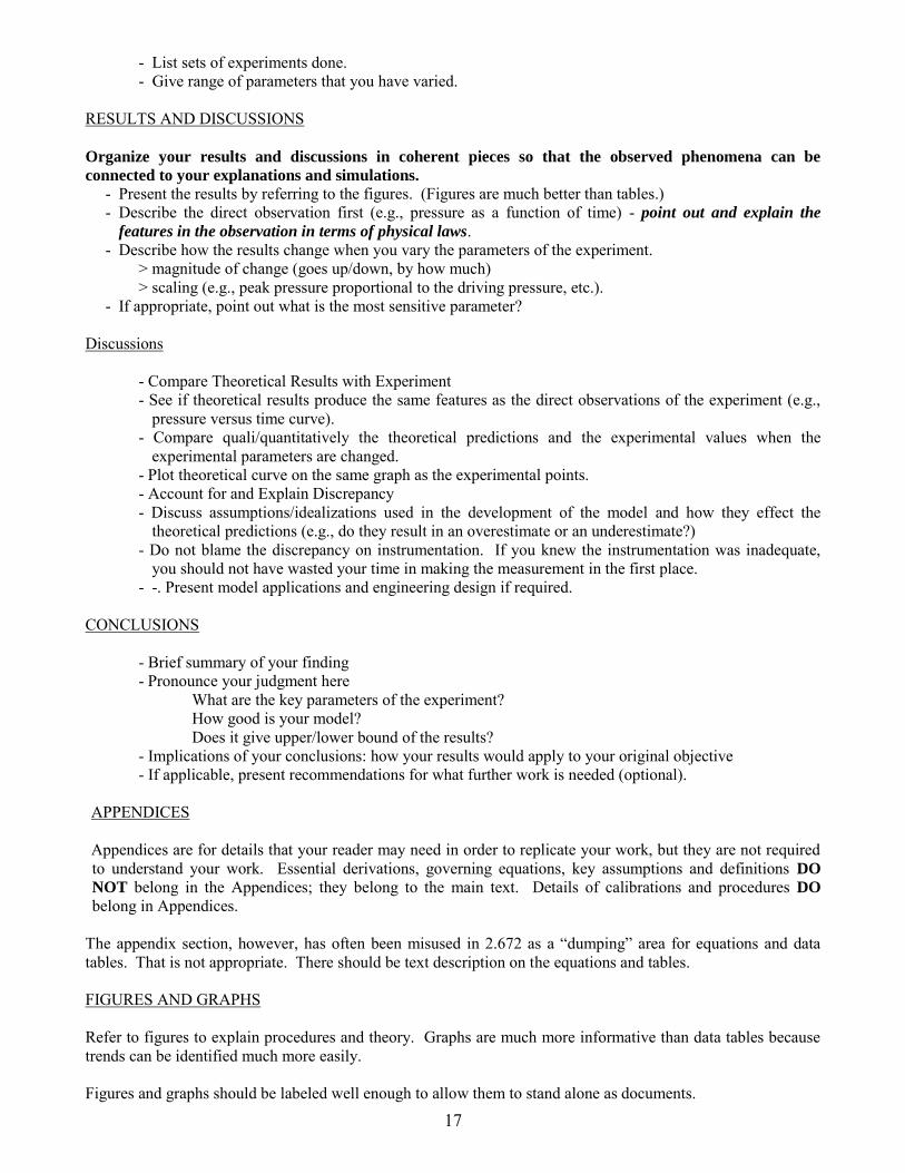
- List sets of experiments done.- Give range of parameters that you have varied.

RESULTS AND DISCUSSIONS

Organize your results and discussions in coherent pieces so that the observed phenomena can be

connected to your explanations and simulations.

- Present the results by referring to the figures. (Figures are much better than tables.) - Describe the direct observation first (e.g., pressure as a function of time) - point out and explain the

features in the observation in terms of physical laws. - Describe how the results change when you vary the parameters of the experiment.

> magnitude of change (goes up/down, by how much)> scaling (e.g., peak pressure proportional to the driving pressure, etc.).

- If appropriate, point out what is the most sensitive parameter?

Discussions

- Compare Theoretical Results with Experiment - See if theoretical results produce the same features as the direct observations of the experiment (e.g.,

pressure versus time curve). - Compare quali/quantitatively the theoretical predictions and the experimental values when the

experimental parameters are changed. - Plot theoretical curve on the same graph as the experimental points. - Account for and Explain Discrepancy - Discuss assumptions/idealizations used in the development of the model and how they effect the

theoretical predictions (e.g., do they result in an overestimate or an underestimate?) - Do not blame the discrepancy on instrumentation. If you knew the instrumentation was inadequate,

you should not have wasted your time in making the measurement in the first place. - -. Present model applications and engineering design if required.

CONCLUSIONS

- Brief summary of your finding - Pronounce your judgment here

What are the key parameters of the experiment?How good is your model?Does it give upper/lower bound of the results?

- Implications of your conclusions: how your results would apply to your original objective - If applicable, present recommendations for what further work is needed (optional).

APPENDICES

Appendices are for details that your reader may need in order to replicate your work, but they are not required to understand your work. Essential derivations, governing equations, key assumptions and definitions DO

NOT belong in the Appendices; they belong to the main text. Details of calibrations and procedures DO

belong in Appendices.

The appendix section, however, has often been misused in 2.672 as a “dumping” area for equations and data tables. That is not appropriate. There should be text description on the equations and tables.

FIGURES AND GRAPHS

Refer to figures to explain procedures and theory. Graphs are much more informative than data tables because trends can be identified much more easily.

Figures and graphs should be labeled well enough to allow them to stand alone as documents.

17

- The physical apparatus for the experiment should be drawn as a schematic and not as a three-

dimensional drawing.

- Results should be presented in graphical form whenever possible. - All figures and graphs should be referred to in text before their appearance. They should all be

numbered.

Graphs 1. Title should be short but informative. It should include what is being graphed and any additional

information needed to interpret the graph. 2. Axes should be labeled (for quantities with dimensions, units are required). 3. Use symbols for data points and lines for theoretical predictions. 4. Each curve should be marked clearly and distinctly.

18

SECTION 4: GUIDE TO ORAL PRESENTATION

GENERAL PRINCIPLES OF TECHNICAL PRESENTATIONS Thomas R. McDonough (MIT ‟66)

1. REHEARSAL Timing - very important Rehearse a speech 10% shorter than the allotted time, since most people speak longer than they expect. If

you exceed allotted time, end quickly. Rehearse beginning and end especially thoroughly. Don‟t memorize the speech word-for-word. Have a

friend critique the rehearsal. Try out the equipment and lighting beforehand. Check for spare projector bulbs 2. ERROR CORRECTIONIgnore the trivial errors of grammar and pronunciation. Don‟t apologize for errors. (Don‟t say “excuse me.”)Apologizing just draws attention to errors.

3.EYES A. Look at audience, not ceiling or floor B. Use visual aids C. Bring in an example of the hardware, if practical.

4.VOICE A. Volume Speak up.

Very important, unless there is a public-address systemSpeak much louder than a conversational tone

B. Quality Don‟t use a boring monotone.Speak slowly and clearly.

5. LANGUAGE A. English: fool everyone into thinking you‟re well educated. Use the best grammar,

enunciation and vocabulary. Avoid: „noises‟ (uh, you know, sort of, kind of, like, ok) „you‟ (e.g., „your electron‟ should be „the electron‟) „thing‟ (e.g., „this thing‟ should be „this device‟) „gonna‟ (say „going to‟)

Slang: A large percentage of technical audiences speaks English as a second language, and many cannot understand slang. Students with strong regional or foreign accents must: put a little . pause . between . each . word. For non technical or interdisciplinary audience: avoid most jargon; define terms carefully.

B. Body Language Don‟t stand stifflyDon‟t move spasmodicallyDo use symbolic gestures

6. ORGANIZATION A. Have three distinct parts:

Beginning (motivation, history, abstract). Tell us: why should anyone care? Middle (body): have a logical order: Tell the story chronologically or start with the

simple and work up to the complex.End: (summary, conclusion, future directions)

B. Keep notes brief. When possible, use visual aids instead of notes. As often as possible, keep notes down and out of sight.

7. ENTHUSIASM (Incredibly important!) From a cover story on Apple/NeXT founder, Steve Jobs, in “Business Week,” 10/24/88: “Of course, Jobs

has a powerful weapon with which to wage these uphill battles: his aura and the notice it attracts. Unsolicited, (Billionaire H. Ross Perot bought 16% of NeXT for $20 million after seeing Jobs‟s infectious enthusiasm on a TV documentary about entrepreneurs. „I‟d be glad to dramatically increase it, too,‟ Perot says.”

19

2.672 ORAL PRESENTATION

As indicated in the course outline, the report for the third lab will be in the form of an oral presentation. In addition to your participation in the oral presentation, you will also be required to hand in, as a group, a copy of the slides used in the oral presentation

PREPARATION OF SLIDES

Each group is expected to prepare their own slides, which YOU will make from the original figures. A projector will be provided, but it is the responsibility of each group to bring a laptop for the presentation. Responsibility for preparation of figures and slides will be a group decision. A good quality paper copy of your slides should also be made and presented to your section instructor at the time of the presentation.

TIME AND LOCATION OF ORAL PRESENTATIONS

Presentations will be held during normal class time. A specific schedule of the presentation (i.e., the time each group presents) will be posted the week prior to the presentation.

Each laboratory group will have a total of 30 minutes for the oral presentation. + Breakdown: 24 minutes for the presentation

6 minutes for questions

Total 30 minutes

PREPARING THE ORAL PRESENTATION

Division of Labor

Be careful that the work is relatively evenly divided among all members of the group. We suggest, but not strongly, the following division of material.

Group of Two Students (12 minutes per student)

1st Student a) Introduction - including overview work b) Experimental Apparatus, Procedure and Results

2nd Student c) Theoretical Model and Results d) Comparison of Theory and Experiment e) Discussion and Conclusions

Students will share answering of questions.

Group of Three Students (8 minutes per student)

1st Student a) Introduction - including overview of work b) Experimental Apparatus, Procedure and Results

2nd Student c) Theoretical Model and Results

3rd Student (d) Discussion and Conclusions

20

SECTION 5: SOFTWARE SUPPORT FOR 2.672 PROJECTS

The 2.672 lab uses the ME computer network system under Window NT. You‟ll log in under a group name and a default password for your lab group (assigned by your instructor). Change the password after you log in the first time. Then you can access the files by logging in on any ME computers.

Computer software packages have been installed in the lab computers for data acquisition, data processing, and word processing. The default directory will be your home directory. The following is a brief overview of these packages.

1. Labview: There are several icons here: CHART, WAVEFORM and VBENCH. CHART is the package

we use the most; it is a general data logging program and displays the data on the fly. You can select which segment of the data you want to store afterwards. WAVEFORM acquires data in the usual way but you cannot display the data until the whole set is taken. VBENCH is a data acquisition virtual bench, which provides simulated oscilloscope, signal generators etc.

2. Matlab: Data processing, data plotting, and numerical simulation software. It has built-in programs for solving differential equations, curve fitting, and signal analysis.

3. Microsoft Word: Word processing software

4. Microsoft Excel: Spreadsheet software

5. Microsoft Powerpoint: Presentation software

21

MATLAB FOR 2.672

This is a short introduction to the MATLAB software. The idea is to enable you to use MATLAB quickly. Refer to the MATLAB REFERENCE MANUAL for more sophisticated operations.

TO USE MATLAB - click the MATLAB icon. It will set up your directory as default for you so that you can access your files.

CONCEPTS

o MATLAB is a giant calculator which remembers the values of all the variables you have calculated. - The command you type in is executed every time you hit a carriage return (CR). Use the up-and-down

arrow keys to recall previous commands. - Sometimes you do not want the intermediate results to be printed (e.g., when you are calculating the

values of a thousand numbers). To do this, end the command with semi-colon, before the CR. - For a very long command that you cannot finish in one line, the line can be continued to the next by using

the ellipsis consisting of three dots..., before the CR.

o One can store a set of commands in a script file and recall it to be used. More of this later in the section SCRIPT FILES. (Using a script file is preferred if you have to do any serious calculations because then you have a record of all the commands you put in, and you can edit them and redo the command sequence easily.)

o If you want to clear your "calculator," use the command CLEAR. You can clear a specific variable by CLEAR variable_name.

o Variables in MATLAB are case sensitive!!! If you prefer, you could adapt the convention of using lower­case characters for scalars and upper-case characters for vectors and matrices.

o MATLAB stands for MATRIX LABORATORY; therefore, the basic representation of information is in terms of matrices. A number, or scalar, is a 1x1 matrix. In 2.672, we mostly deal with vectors (e.g., an array of data). Because the software is matrix-based, there can be quite a bit of confusion if you are not careful. For example, if x is a 5x1 matrix (i.e., a column vector of 5 elements), X*X is illegal. On the other hand X*X' (X' stands for the transpose of X) will give you a scalar.

o You can always click the HELP icon to search for information within MATLAB.

BASIC OPERATIONS

o The operators +,-,*,/,^ have the usual meaning. (The last one is to raise power.) - operation between a scalar (s) and a matrix (A) is straight forward; e.g. s*A means that every element of A

is multiply by s. - For operations between matrices (vectors are special case of matrices: a row vector of n elements is a nx1

matrix; a column vector is a 1xn matrix), you have to be careful that the dimensions match, or you will get error messages.

- Division means multiplication by the inverse matrix. As such, there are two different symbols: the right division, e.g. A/B = A*B-1, and the left division, e.g. C\D = C-1*D.

- In most of the applications, we want to do element-by-element operation. To do this, precede the

operator by a dot. e.g. If X=[1,2,3] and Y=[2,4,6]. Then X*Y is illegal, but X .*Y=[2,8,18]. Use X . ^2 to obtain the square of the elements of X in the above example.

o Complex numbers - Numbers can be complex. When you first start MATLAB, (or after a CLEAR command,) the symbols i and j are given the value of sqrt(-1). Thus you can enter complex numbers such as x=4+5*i. (In this case, because you are entering a pure number instead of an expression, you do not have to use the multiplication sign, thus x=4+5i or x= 4+5j are valid.) (Think about applications when you have to do

22

complex transfer functions.) If you have used i and j for some other things, you can recreate them by setting i=sqrt(-1) etc.

o To access the elements of a vector - For vector X (does not matter whether it is a column or row vector), X(n) is the nthelement of X.

o To access the elements of a matrix - For matrix A, A(m,n) refers to the element in the mthrow and the nth column.

o The range operator (:) - It is convenient to be able to refer to a range of elements. The colon symbol does that. e.g. for a vector X, V=X(3:5) is a vector (row or column vector, corresponding to that of X) of length 3, with V(1)=X(3), V(2)=X(4), V(3)=X(5). Similarly for a matrix A, A(2,7:9) refers to the second row, and elements A(2,7), A(2,8),A(2,9).

o The extremely useful expression is the range operator without range specification. Then, it refers to the whole range. For example A(:,3) refers to the third column of the matrix A, and B(2,:) refers to the second row of A.

o There are a lot of other useful operations such as looping, logical test, etc. which are not described in here. Refer to the manual or the on-line HELP if you need to use them. To learn about looping, type HELP FOR; to learn about logic test, type HELP IF.

BUILT-IN FUNCTIONS

There are many built-in functions, such as all the standard ones (sin, cos, tan, exp, sqrt etc.) and many special ones, such as quad (to integrate a function by quadrature). In addition, we have prepared several functions for the 2.672 lab, such as steam_p (to evaluate the saturated thermodynamic properties of water for an input pressure) and fitplot (to fit a polynomial of nth degree to data and plot the data as points and the fit as line). See the MATLAB REFERENCE MANUAL for listing of built-in functions, or click the HELP icon for on-line listing. A short listing of the 2.672 built-in functions can be found at the end of this manuscript.

ENTERING NUMBERS BY HAND

o Scalar. Entering a scalar is obvious, e.g., s=5.

o Row Vector. To enter a row vector, start off with the left square bracket and end with the right square bracket. For example, X=[1,2,3,4,5] is a 1x5 vector. If it is a very long vector, use the ... line continuation method.

o Column Vector. To enter a column vector, the method is similar to the row vector, except that the elements are separated by semi-colons instead of commas. For example, Y=[2;4;6;8] is a 4x1 vector. Another way to do this is to use the transpose operator; i.e., enter as Y=[2,4,6,8]‟.

o Range Operator. The range operator (:) is very useful for entering numbers. For example: X=[1:5] is the vector [1,2,3,4,5]. Even more useful, is the range with increment specification, i.e., start:increment:end. For example, Y=[0:0.2:1] is the vector [0,0.2,0.4,0.6,0.8,1.0]. The latter construction is very useful if you want to specify a range to calculate a function (e.g., the range of frequency to calculate the transfer function).

o Matrix. Entering the values of the elements of a matrix can best be illustrated by an example. X=[1,2,3

4,5,6]

is the 2x3 matrix. Alternatively, you can enter it as X=[1,2,3;4,5,6], with the rows separated by the semicolon. Note that the construction is consistent with that of the row and column vectors.

23

IMPORTING DATA FILES FROM THE DATA ACQUISITION SYSTEM

In the data acquisition package, choose to save the data in the matlab format. Give it a file name, for example xyz (the first character of the filename should be non-numeric; do not use any extension, because the default extension is .m). Then go to the MATLAB window and type in the filename as a command; in this case, it is xyz. The data will be imported. The data will also be plotted. Use the command whos to find out what are the data variable names.

Often you want to pick off values from the plot. The following command reads off n points on the plot and puts the coordinates into arrays x and y.

[x,y]=ginput(n)

You have to enter a value for n. For example, if you enter [x,y]=ginput(4), a cross-hair will appear on the figure of the plot. Use the mouse to locate the cross-hair on your curve. Clicking the mouse will enter the coordinate of the cross-hair into x and y. Repeat the process four times to finish the command and get four pair of coordinates in the arrays x and y. Note that the process does not terminate until all n points are done. (To kill the process, use ctl-c.)

To access the variables in the acquired data, use the function getdata which can be downloaded from the 2.672 web page. After you download it to your working directory, type help getdata to learn how to use the function.

PLOTTING

The strategy is to create the plot (using auto-scaling) first, and to rescale the axes if necessary, add titles, axes labels etc. later. The plot appears in another window called "Figure 1" (and "Figure 2" etc. if you have more than one plot). To print the graph, go to this window and click the file icon. See later for option to import the graph to Microsoft Word document.

The plot command creates a 2D plot of vectors or matrices. Use plot(X,Y) to plot vector X versus vector Y. If X or Y is a matrix, the vector is plotted versus the rows or columns of the matrix, whichever line up.

plot(Y) plots the columns of Y versus their index. If Y is complex, plot(Y) is equivalent to plot(real(Y),imag(Y)). In all other uses of plot, the imaginary part is ignored.

Various line types and plot symbols may be obtained with plot(X,Y,S) where S is a character enclosed in ' ' selecting the plot style as follows:

. point - solid line o circle : dotted linex x-mark -. dash-dot line+ plus -- dashed line * star

For example, plot (X,Y,'o') plots a circle symbol at each data point, and plot(X,Y,'-') connects the data pointswith a solid line.

plot (X1,Y1,S1,X2,Y2,S2,X3,Y3,S3,...) combines the plots defined by the (X,Y,S) triples, where the X's and Y's are vectors or matrices and the S's are strings. X1,Y1,S1 are for the first plot; X2,Y2,S2 are for the second; etc.

Now that you have the plot, you can make it look nice by the following commands:

To re-scale the axis, use the command axis([xmin, xmax, ymin,ymax]). Note that the [ ] is necessary becausethe argument to the function AXIS is actually a 1x4 vector. You may use the functions xlim and ylim to set thex and y axis limits respectively.To add axes labels and title, use xlabel('text'), ylabel('text') and title('text').

24

Use gtext(„text‟) to add text any where on the graph. A cross-hair will show up. Use the mouse to move it toposition and click.To create a log-log plot, substitute the command plot (...) by logplot (...). Similar substitutions are used forsemilogx, and semilogy.

See the manual or use the HELP icon for more advance topics such as multiple plots on a page (SUBPLOT),overlaid plots (HOLD), and freezing the axes scales etc. You can also use the edit manual to make the linesthicker etc.

FITPLOT - Many times, one has to fit a curve to data points. This procedure is done by a 2.672 built-infunction.

C=fitplot(X,Y,n) fits a nth degree polynomial to the data, and plot the data points as circles and the fit as a solidline. The fit coefficients are put in the vector C in order of descending powers. For example C=fitplot(X,Y,1)would do a linear fit, with y=C(1)*x+C(2).

Often you have to look at the exponential decay coefficient of y as a function of t. The command:C = fitplot(T,LOG(Y),1)

will do the trick. The information is then in C(1).

TO IMPORT GRAPHS TO MICROSOFT WORD DOCUMENT

If you want your graph to appear as a picture in the Word document, first create the graph in Matlab, and copy it using the edit menu. Then the graph is copied onto the clipboard as a Window metafile ready to be pasted onto a Word document.

SCRIPT FILES

These are files containing commands that you can recall to reuse again and again. These files have to have the file extension .m.

To create them, click the file icon, follow by the new icon, and then follow by the M_file icon. Then the Matlab editor will come up, and you can type in your commands. Afterwards hit the file icon; follow by the save as icon. You'll be asked for the filename etc. Save the file with extension .m. After successfully saving what you have typed in the file, the program will return to the editor. Then click the file icon again, and click exit.

To edit a previous file, click the file icon; follow by the open m file icon. Then the procedure is as in the above.

There are two kinds of script files:

The command script files--This is a collection of commands. To invoke them in a MATLAB session, type in the filename of the script file (without extension, because the default extension is .m). Then all the commands in the file will be inserted and executed.

Hints- (a) It is useful to document your script file with comments. Anything starting with a % symbol is a comment. The comment could either start at the beginning or anywhere in a line.

(b) Usually, you don't want the intermediate results to be displayed. End the commands with ; in the script file.

The function subroutine script files - These are files that you can call within a MATLAB command as a function. The filename in which the function subroutine is stored must be the same as the function name (i.e., name in the following), with the extension .m. The first line of these files must be:

25

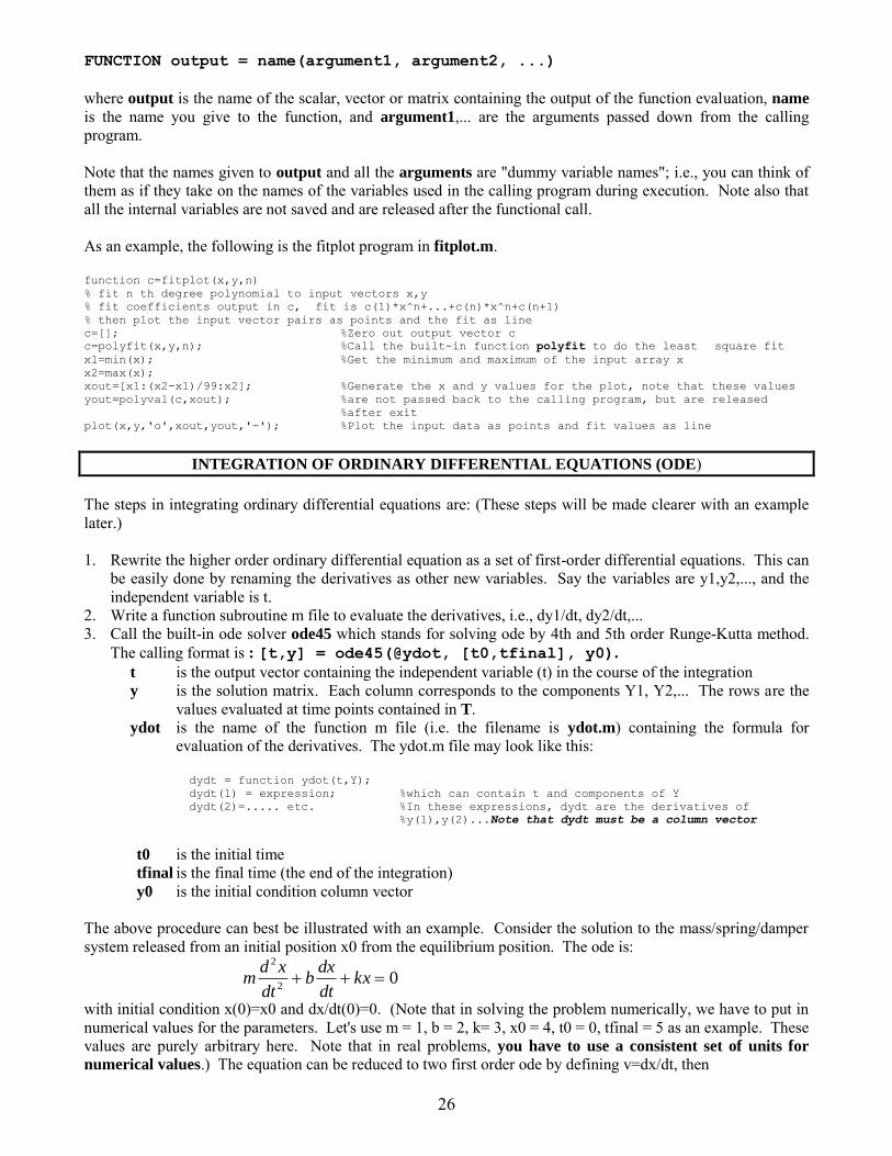
FUNCTION output = name(argument1, argument2, ...)

where output is the name of the scalar, vector or matrix containing the output of the function evaluation, name

is the name you give to the function, and argument1,... are the arguments passed down from the calling program.

Note that the names given to output and all the arguments are "dummy variable names"; i.e., you can think of them as if they take on the names of the variables used in the calling program during execution. Note also that all the internal variables are not saved and are released after the functional call.

As an example, the following is the fitplot program in fitplot.m.

function c=fitplot(x,y,n)

% fit n th degree polynomial to input vectors x,y

% fit coefficients output in c, fit is c(1)*x^n+...+c(n)*x^n+c(n+1)

% then plot the input vector pairs as points and the fit as line

c=[]; %Zero out output vector c

c=polyfit(x,y,n); %Call the built-in function polyfit to do the least square fit

x1=min(x); %Get the minimum and maximum of the input array x

x2=max(x);

xout=[x1:(x2-x1)/99:x2]; %Generate the x and y values for the plot, note that these values

yout=polyval(c,xout); %are not passed back to the calling program, but are released

%after exit

plot(x,y,'o',xout,yout,'-'); %Plot the input data as points and fit values as line

INTEGRATION OF ORDINARY DIFFERENTIAL EQUATIONS (ODE)

The steps in integrating ordinary differential equations are: (These steps will be made clearer with an example later.)

1. Rewrite the higher order ordinary differential equation as a set of first-order differential equations. This can be easily done by renaming the derivatives as other new variables. Say the variables are y1,y2,..., and the independent variable is t.

2. Write a function subroutine m file to evaluate the derivatives, i.e., dy1/dt, dy2/dt,... 3. Call the built-in ode solver ode45 which stands for solving ode by 4th and 5th order Runge-Kutta method.

The calling format is : [t,y] = ode45(@ydot, [t0,tfinal], y0).

t is the output vector containing the independent variable (t) in the course of the integration y is the solution matrix. Each column corresponds to the components Y1, Y2,... The rows are the

values evaluated at time points contained in T. ydot is the name of the function m file (i.e. the filename is ydot.m) containing the formula for

evaluation of the derivatives. The ydot.m file may look like this:

dydt = function ydot(t,Y);

dydt(1) = expression; %which can contain t and components of Y

dydt(2)=..... etc. %In these expressions, dydt are the derivatives of

%y(1),y(2)...Note that dydt must be a column vector

t0 is the initial time tfinal is the final time (the end of the integration) y0 is the initial condition column vector

The above procedure can best be illustrated with an example. Consider the solution to the mass/spring/damper system released from an initial position x0 from the equilibrium position. The ode is:

md x

dtb

dx

dtkx

2

20

with initial condition x(0)=x0 and dx/dt(0)=0. (Note that in solving the problem numerically, we have to put in numerical values for the parameters. Let's use m = 1, b = 2, k= 3, x0 = 4, t0 = 0, tfinal = 5 as an example. These values are purely arbitrary here. Note that in real problems, you have to use a consistent set of units for

numerical values.) The equation can be reduced to two first order ode by defining v=dx/dt, then

26

____________________________________________________________________________________

dx/dt = v, anddv/dt = -(bv+kx)/m

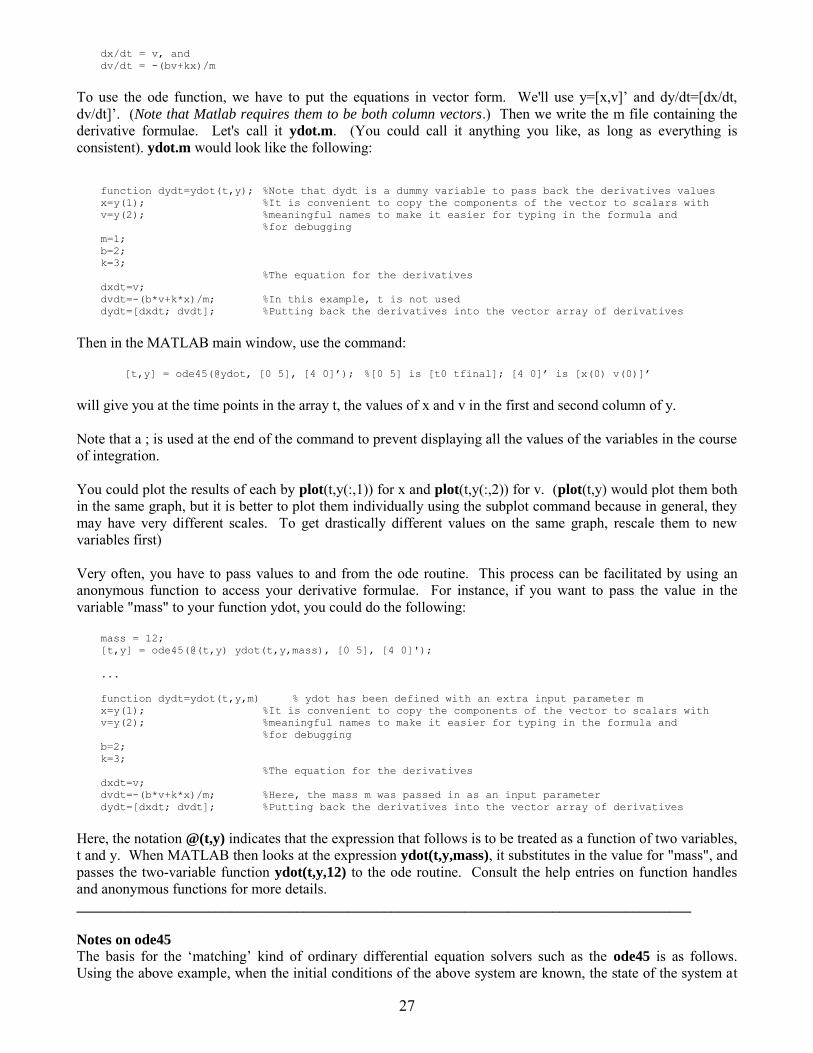
To use the ode function, we have to put the equations in vector form. We'll use y=[x,v]‟ and dy/dt=[dx/dt, dv/dt]‟. (Note that Matlab requires them to be both column vectors.) Then we write the m file containing the derivative formulae. Let's call it ydot.m. (You could call it anything you like, as long as everything is consistent). ydot.m would look like the following:

function dydt=ydot(t,y); %Note that dydt is a dummy variable to pass back the derivatives values

x=y(1); %It is convenient to copy the components of the vector to scalars with

v=y(2); %meaningful names to make it easier for typing in the formula and

%for debugging

m=1;

b=2;

k=3;

%The equation for the derivatives

dxdt=v;

dvdt=-(b*v+k*x)/m; %In this example, t is not used

dydt=[dxdt; dvdt]; %Putting back the derivatives into the vector array of derivatives

Then in the MATLAB main window, use the command:

[t,y] = ode45(@ydot, [0 5], [4 0]’); %[0 5] is [t0 tfinal]; [4 0]’ is [x(0) v(0)]’

will give you at the time points in the array t, the values of x and v in the first and second column of y.

Note that a ; is used at the end of the command to prevent displaying all the values of the variables in the course of integration.

You could plot the results of each by plot(t,y(:,1)) for x and plot(t,y(:,2)) for v. (plot(t,y) would plot them both in the same graph, but it is better to plot them individually using the subplot command because in general, they may have very different scales. To get drastically different values on the same graph, rescale them to new variables first)

Very often, you have to pass values to and from the ode routine. This process can be facilitated by using an anonymous function to access your derivative formulae. For instance, if you want to pass the value in the variable "mass" to your function ydot, you could do the following:

mass = 12;[t,y] = ode45(@(t,y) ydot(t,y,mass), [0 5], [4 0]');

...

function dydt=ydot(t,y,m) % ydot has been defined with an extra input parameter m

x=y(1); %It is convenient to copy the components of the vector to scalars with

v=y(2); %meaningful names to make it easier for typing in the formula and

%for debugging

b=2;

k=3;

%The equation for the derivatives

dxdt=v;

dvdt=-(b*v+k*x)/m; %Here, the mass m was passed in as an input parameter

dydt=[dxdt; dvdt]; %Putting back the derivatives into the vector array of derivatives

Here, the notation @(t,y) indicates that the expression that follows is to be treated as a function of two variables, t and y. When MATLAB then looks at the expression ydot(t,y,mass), it substitutes in the value for "mass", and passes the two-variable function ydot(t,y,12) to the ode routine. Consult the help entries on function handles and anonymous functions for more details.

Notes on ode45

The basis for the „matching‟ kind of ordinary differential equation solvers such as the ode45 is as follows. Using the above example, when the initial conditions of the above system are known, the state of the system at

27

every next time step, x(t+t) and v(t+t), can be predicted from its current state, x(t), v(t) and their derivatives. In this case:

dx/dt = v(t)dv/dt = a(t), wherea(t)= -(b(t)*v(t)+k*x(t))/m,

The time-marching solution process can be illustrated by a first-order-accuracy numerical scheme,

x(t+t)=x(t)+v(t)*t, andv(t+t)=v(t)+a(t)*t.

In ode45, the above time-marching solution is obtained with a higher order of accuracy. It is based on the fourth- and fifth-order Runge-Kutta method. See a numerical analysis text book for detailed description of the algorithm.

28

____________________________________________________________________________________

LIST OF MATLAB APPLICATION PROGRAMS FOR 2.672 PROJECTSThe following Matlab programs have been prepared for 2.672 projects. These programs can be run in

the Matlab main window or be called in script files.

Detailed information about these programs can be obtained in the Matlab main

window by entering

help function name <return>

The m files for these programs are also available for your personal use via download from the 2.672 web page. You may copy them for your own use outside the lab.

Function Name Description fitplot Fit a nth degree polynomial to the data, plot the data points as circles and the fit as a

solid line ginput Matlab intrinsic function for getting the coordinates of points on a graph with a

cursor getdata Loads data from the 2.672 chart program to designated variables pwrspect Transform data from the time domain to the frequency domain, and find an

oscillation frequency. The peak location in the power spectrum is printed. powerfit Least squares fit of data using a linear combination of powers. A particular use is to

fit a straight line with a forced fit through the origin steam_p Calculate the thermophysical properties of saturated water for a given temperature;

output saturation pressure and properties steam_t Calculate the thermophysical properties of saturated water for a given pressure;

output saturation temperature and properties H2Oprop Calculate the thermophysical and/or transport properties of water at any given

thermodynamic state

29