PHYS 652: Astrophysics 143

26 Lecture 26: Galaxies: Numerical Models

“All science is either physics or stamp collecting.”Ernest Rutherford

The Big Picture: Last time we derived the collisionless Boltzmann equation in the context ofgalaxies, formulated the self-consistent problem and outlined a few analytical approaches to solvingit. In search of a physically more faithful model of realistic galaxies, today we talk about numericalsimulations. We outline the main approaches, along with their advantages and disadvantages.

Numerical Simulations of Galaxies

Realistic galaxy models — which often include non-integrable and time-dependent potentials in3 dof — are not analytically tractable. Numerical simulations are our only hope in understandingthe fundamental aspects of the underlying dynamics of these systems, such as:

• the non-linear collective phenomena leading to small-scale structure (central cusps, globularclusters, bars, arms, etc...);

• mechanisms which drive the system toward equilibrium;

• correlation between physical properties of the galaxy (size, luminosity, mass of the centralsupermassive black hole, velocity dispersion, etc...), as hints about the galaxy evolution.

The numerical techniques invoked in simulating galaxies differ in their implementation of thephysical problem. N-body simulations attempt to solve the physical problem in a direct way: parti-cles interacting with each other via gravitational 1/r2 force. The Schwarzschild orbit superposition

method assumes time-independent system (in equilibrium), and solves the self-consistent problem.Distinguishing between numerical artifacts and physics intrinsic to these multiparticle systems be-comes a major challenge. We now discuss each one of these approaches in some detail.

N-Body Simulations

In N-body simulations, the N “macroparticles” sampling the initial DF are evolved under eachother’s gravitational influence. Implementing a perfectly faithful representation of the physicalsystem is computationally prohibitive because of the two main reasons:

1. Size of the system: the number of “particles” (stars) in a realistic galaxy is huge: N ≈ 1012;

2. Scaling of the interaction: because gravity is a force with an infinite range each star ”feels”gravitational force due to each other star in the system, which means that the number ofinteractions scales as O(N2).

The three main types of N-body codes: (i) direct summation, (ii) tree, and (iii) particle-in-cell,invoke different approximations to deal with these problems.

Direct summation samples the initial DF by Npart macroparticles and evolves them via particle-to-particle interaction.

• Advantage: The implementation is closest to the physical problem (individual particles inter-acting with each other).

143

PHYS 652: Astrophysics 144

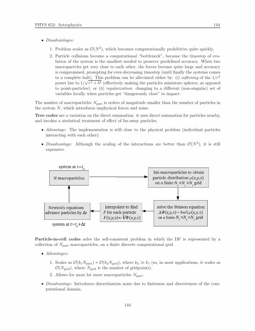
• Disadvantages:

1. Problem scales as O(N2), which becomes computationally prohibitive quite quickly.

2. Particle collisions become a computational “bottleneck”, because the timestep of evo-lution of the system is the smallest needed to preserve predefined accuracy. When twomacropartcles get very close to each other, the forces become quite large and accuracyis compromised, prompting for ever-decreasing timestep (until finally the systems comesto a complete halt). This problem can be alleviated either by: (i) softening of the 1/r2

power law to 1/√

r4 + b4 (effectively making the particles miniature spheres, as opposedto point-particles); or (ii) regularization: changing to a different (non-singular) set ofvariables locally when particles get “dangerously close” to impact.

The number of macroparticles Npart is orders of magnitude smaller than the number of particles inthe system N , which introduces unphysical forces and noise.

Tree codes are a variation on the direct summation: it uses direct summation for particles nearby,and invokes a statistical treatment of effect of far-away particles.

• Advantage: The implementation is still close to the physical problem (individual particlesinteracting with each other).

• Disadvantage: Although the scaling of the interactions are better than O(N2), it is stillexpensive.

Particle-in-cell codes solve the self-consistent problem in which the DF is represented by acollection of Npart macroparticles, on a finite discrete computational grid.

• Advantages:

1. Scales as O(k1Npart) +O(k2Ngrid), where k2 ≫ k1 (so, in most applications, it scales asO(Ngrid), where Ngrid is the number of gridpoints).

2. Allows for more lot more macroparticles Npart.

• Disadvantage: Introduces discretization noise due to finiteness and discreteness of the com-putational domain.

144

PHYS 652: Astrophysics 145

Recently, the Beam Physics and Astrophysics Group at NICADD has been involved in developinga new variant of particle-in-cell solvers which use wavelets to remove some of the numerical noiseintrinsic to the method (http://www.nicadd.niu.edu/∼bterzic/Research/TPB 2007.pdf).

Schwarzschild’s Orbit Superposition Method

Figure 44: Flow-chart for modeling galaxies using Schwarzschild’s method. The referenceis Chandrasekhar 1969, Ellipsoidal Figures of Equilibrium, Dover, New York. For detailson modeling individual galaxies by fitting them to a new family of mass-density profiles, seehttp://www.nicadd.niu.edu/∼bterzic/Research/TG 2005.pdf.

Schwarzschild’s orbit superposition method divides the model into cells of a 3D sphere. Basedon the amount of time it spends in each of the cells i, the orbital density template ρij for eachorbit is computed. Now, we seek the set of non-negative weights wi for each of the orbits, suchthat the weighted sum of all the orbital densities of the model will reproduce the starting densitydistribution of the model ρi in each of the i cells. That is,

ρi =

No∑

j=1

wjρij, (544)

where No is the number of orbits and the normalized orbital densities are given by

1 =

Nc∑

i=1

ρi, (545)

with Nc being the number of cells in a 3D sphere. Equations (544) and (545) constitute an op-timization problem and can be solved in several ways, the most popular of which are the linearprogramming or least squares methods.

145

PHYS 652: Astrophysics 146

Optimization problem.Schwarzschild’s method is formulated as an optimization problem:

minimize : f (wi),

subject to :No∑

i=1wi ρij = ρj, j = 1, 2, ..., Nc, (546)

wi ≥ 0, i = 1, 2, ..., No ,

where f(wi) is the cost function, ρij is the contribution of the orbital density of the ith template tojth cell, ρj is the model’s density in the jth cell and wi is the orbital weight of the ith orbit. Theproblem above becomes a linear programming problem (LPP) when the cost function is a simple lin-ear function of the weights; for example, to minimize weights of orbits labeled from m to n, the cost

function would simply be f(wi) =n∑

i=mwi. The solutions of the LPP are often quite noisy, with entire

ranges of orbits carrying zero weights. It is often customary to impose additional constraints in or-der to “smoothen” out the solutions, such as minimizing the sum of squares of orbital weights (whichmakes this a quadratic programming problem) or minimizing the least squares. (For an pedagogicaland detailed discourse on the implementation of the Schwarzschild’s method for a special case ofscale-free potentials, see http://www.nicadd.niu.edu/∼bterzic/Research/chapter3.pdf).Chaotic orbits.The orbital density templates ρij are computed so as to represent the time-averaged orbital densityof stars on that orbit, thus making them time-independent building blocks of a time-independentsolution to the self-consistent problem. Chaotic orbits (to be defined later in this lecture) cannot

have their individual orbital density templates included into Schwarzschild’s method because theirtime-averaged density would change over time. Instead, chaotic orbits are usually averaged out intoa single chaotic super-orbit orbital template and then included in Schwarzschild method. This isbecause chaotic portion of the phase space in 3 dof (and higher) are interconnected (Arnold’s web),so all chaotic orbits in a given potential can be viewed as parts of one large chaotic super-orbit (i.e.,if integrated long enough — infinitely long — each chaotic orbit will sample all of the availablechaotic phase-space).

Chaos in Galactic Simulations

Decades of numerical simulations have shown that realistic galactic models feature a large num-ber of chaotic orbits. As a case in point, even simple dynamical systems such as the gravitational(restricted) three-body problem features a large portion of chaotic orbits. Another example is anumerical simulation of a 10-body model of a solar system, which found e-folding times for eachof the planets’ orbits in the range of 10 − 50 million years (Laskar 1993, Physica D, 67, 257). Itis then quite reasonable to expect that N-body simulations for which N ≫ 10 will feature chaoticorbits.

In simulations which smooth over particle distribution by invoking a mean-field approximation,such as integration of orbits in a smooth potential, presence of chaos is not nearly as obvious. Thepresence of chaos has only been discovered after the integration of orbits revealed that the numberof integrals of motion was fewer than the number of degrees of freedom (Henon & Heiles 1963,Astronomical Journal, 69, 73).

Definition of chaos: Motion which exhibits sensitive dependence on initial conditions.In other words, nearby orbits will diverge exponentially:

d(t) = d(0)eλt, (547)

146

PHYS 652: Astrophysics 147

where d(0) is the initial separation of nearby orbits, d(t) is the separation of initially nearby orbitsat some later time t, and λ is the Lyapunov exponent.

The Lyapunov exponent is defined as

λ = limt→∞, d(0)→0

1

tln

d(t)

d(0), (548)

and is related to the “e-folding time” τe as τe = 1/λ. The e-folding time denotes a time-scaleafter which one can no longer make quantitative predictions about the system. In other words —loosely speaking — it is the time-scale after which the motion on the same orbit will be completelyuncorrelated.

Here a note of caution is appropriate: the colloquial use of the term “chaotic” has led toa common misconception that chaos implies complete randomness. This is not the case: chaosimplies intrinsic inability to quantify the system beyond the e-folding time.

Regular motion is characterized by vanishing Lyapunov exponents. Orbits are well-defined, havelocalized Fourier spectra, and “appear” regular (”quasi-periodic”). Regular motion in an N -dofsystem is confined by its three integrals of motion to the surface of the N -dimensional torus residingin the 2N -dimensional phase-space.

Chaotic (stochastic, irregular) motion is characterized by non-zero Lyapunov exponents. Or-bits are not well-defined, have “fuzzy” Fourier spectra, and generally “appear” irregular, but notalways: “weakly chaotic” or “sticky” orbits can mimic regular behavior for long periods of time,only to become “wildly chaotic” at later times (short-time Lyapunov exponents can vary drasti-cally). Chaotic motion in an N -dof system is not confined to the surface of the N -dimensionaltorus residing in the 2N -dimensional phase-space, because it does not have N integrals of motion.

Integrable potential have as many integrals of motion as the degrees of freedom. All orbits areregular. Examples of integrable potentials include all spherically symmetric systems (there is nochaos in 1D) and some axisymmetric potentials (2 dof).

Non-integrable potential do not have as many global integrals of motion as the degrees offreedom. However, the presence of local integrals of motion is possible, so there are generally bothchaotic and regular orbits.

Relaxation of Multiparticle Systems

Earlier we computed time needed for the system to reach equilibrium (relaxation time) throughcollisions (close encounters) to be orders of magnitude longer than the Hubble time. This meansthat if close encounters was the only relaxation mechanism at work, we should observe galaxies tobe far from equilibrium. Observations show the contrary: galaxies are to a good approximationrelaxed systems, in (or at least close to) equilibrium. It then became clear that there are othermechanisms at work in driving the system toward equilibrium.

There are several mechanisms believed to be at work in galactic systems, as seen in copiousnumerical studies.

Regular phase mixing (Landau damping) is present in both time-independent and time-dependent systems. It causes ensembles of regular orbits to spread out because of initial spread intheir integrals of motion. If one imagines that nearby orbits reside on slightly different tori, theirconsequent evolution along the surfaces of their respective tori will result in their shear separation(Fig. 46, top panel). The timescale for regular phase mixing depends on: (i) the size of the ensemble

147

PHYS 652: Astrophysics 148

z

y

z

x

y

x

z

y

z

x

y

x

z

y

z

x

y

x

z

x

y

x

z

y

a) b) c) d)

z

y

z

x

y

x

z

y

z

x

y

x

z

y

z

x

y

x

z

x

y

x

z

y

e) f) g) h)

Figure 45: Some of the most common orbits in scale-free potentials. Major orbital families: a) regularbox, b) chaotic box, c) regular long-axis tube, d) regular short-axis tube. Minor resonant families: e) x-yfish, f) x-z fish, g) x-y pretzel, h) x-z pretzel. (From Terzic 2002, PhD thesis, Florida State University.http://www.nicadd.niu.edu/∼bterzic/Research/dissertation.pdf).

148

PHYS 652: Astrophysics 149

in phase space; (ii) crossing time for the ensemble. Generally speaking, regular phase mixing isnot a very powerful mechanism, but is the only mechanism driving the integrable systems towardequilibrium.

Chaotic phase mixing (non-linear Landau damping) occurs in both time-independent andtime-dependent systems. Numerical simulations show that a microscopic ensemble of isoenergetictest particles in a realistic galaxy potential around a chaotic orbit will mix on timescales t ∼30 − 100tcross. The ensemble will evolve to uniformly fill the isoenergy surface accessible to it. Insystems in which a large fraction of the phase-space is occupied with chaotic orbits, chaotic mixingcould be an important mechanism for driving secular evolution on timescales much shorter thantcollision (Lynden-Bell 1967, MNRAS, 136, 101; Merritt & Valluri 1996, Astrophysical Journal, 471,82).

Figure 46: Regular phase mixing (top) and chaotic phase mixing (bottom). (From Merritt & Valluri 1996,Astrophysical Journal, 471, 82)

Violent relaxation occurs only in time-dependent potentials. According to the virial theorem

1

2

d2I

dt2= 2T + V, (549)

so that 2T/V = 1 for a self-gravitating system in dynamical equilibrium. A system out of equilib-rium will undergo oscillations during which the particles will exchange energy with the background

149

PHYS 652: Astrophysics 150

Figure 47: Chaotic phase mixing. (From Merritt & Valluri 1996, Astrophysical Journal, 471, 82)

potential:

dE

dt= −dΦ

dt

Tr =

⟨

(

dEdt

)2

E2

⟩

−1/2

=

⟨

(

dΦdt

)2

E2

⟩

−1/2

(550)

which leads to (Lynden-Bell 1967, MNRAS, 136, 101)

Tr ≃ 3P

8π, (551)

where P is the typical radial period of the orbit of a star. The violently changing gravitational fieldof a newly formed galaxy is effective in driving the stellar orbits toward equilibrium on timescalesmuch shorter that the Hubble time. For a discussion of orbital structure — both regular andchaotic — in time-dependent galactic potentials modeling conditions during violent relaxation, seehttp://www.nicadd.niu.edu/∼bterzic/Research/TK 2005.pdf.

150