2.5D Finite Element Simulation Eddy Current Heat …repository.uwtsd.ac.uk/683/1/Pullen, A. and Charlton, P. (2015) 2... · 2.5D Finite Element Simulation – Eddy Current Heat Exchanger

Vol.20 No.7 (July 2015) - The e-Journal of Nondestructive Testing - ISSN 1435-4934 www.ndt.net/?id=18011

1

2.5D Finite Element Simulation – Eddy Current Heat Exchanger Tube

Inspection using FEMM

Ashley L. PULLEN, Peter C. CHARLTON

Faculty of Applied Design and Engineering, University of Wales Trinity Saint David; Swansea, Wales, UK;

Phone: +44(0)1792 481000; e-mail: [email protected], [email protected]

Abstract

The paper describes the use of the open source electromagnetic finite element software package, FEMM used to

simulate heat exchanger eddy current tube inspection. The paper provides an understanding of eddy current

impedance plane responses to a number of defects using 2.5D axisymmetric finite element analysis. The

scenarios examined are; corrosion, internal and external defects, baffle plate and baffle plate with fretting

responses, internal defect, lift-off or improper fit and tube exit responses. A mathematical method of estimating

the eddy current density as a function of penetration depth is also investigated with less than 5% over estimation.

Finite element mesh optimisation is also investigated and a trade-off is made between accuracy and simulation

time. Background knowledge on basic eddy current and heat exchangers is provided in the opening sections of

the paper. Probe frequency variation and optimisation along with mesh boundaries are also discussed to help

improve the simulation method. The effects of altering inspection frequency and the multiple effects this has on

the inspection process are also discussed throughout the paper.

Keywords: Eddy Current, Tube Inspection, Finite Element Simulation, FEMM, Heat Exchanger Inspection,

Eddy Current Skin Depth Penetration, Current Density, Mesh Optimisation, Phase Angle, Finite Element

Analysis

1. Introduction Eddy current inspection (ECT) has become the most widely used Non-Destructive Testing

(NDT) methods for heat exchanger tube inspection. This paper discusses a finite element

parametric study for a simulated heat exchanger inspection process using 100% IACS copper

winding for the Eddy Current (EC) coil along with the heat exchanger. The study includes

impedance plane diagrams to illustrate the effects that defect orientation and depth have on

the eddy current coils phase angle and impedance.

Prior to the analyses process mesh optimisation is undertaken; this ensures an optimisation

between result accuracy and computational time. Probe frequency optimisation is also

considered.

The simulation of Eddy Current (EC) penetration depth and its relationship with frequency is

analysed. A numerical approach in approximating the surface current density is also

investigated with values extrapolated from the simulated results, coupled with the EC

penetration depth formula where the Eddy Currents are 36.7% or 1/e of its surface value.

A simulation of insufficient probe fit is also investigated along with the effects of tube

supports that are normally in place to enforce and support heat exchanger tubes. Multiple

defect situations are also discussed and their impedance plane responses shown to aid in the

understanding of EC impedance plane responses and the likely defect that is causing such a

response.

2. Informative Literature 2.1 Eddy Current Probe

Eddy Current probes use the physics phenomenon of electromagnetic induction. In an EC

probe an alternating current flows through a wire coil in turn generating an oscillating


2

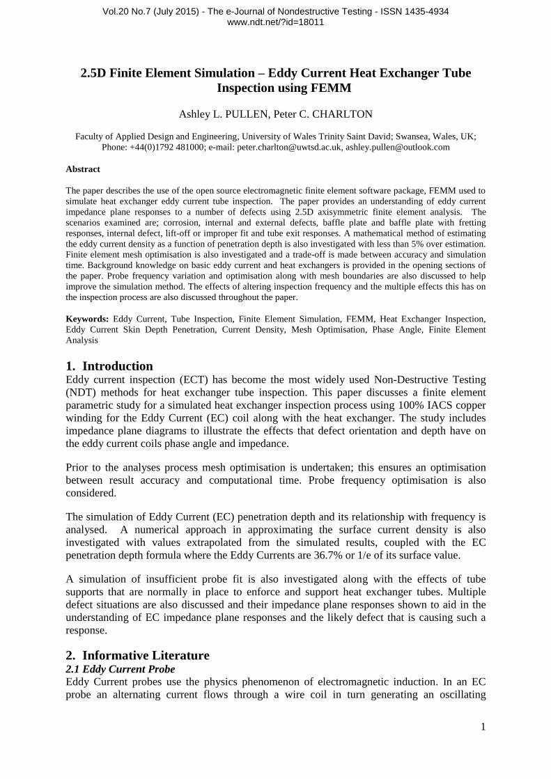
magnetic field. If the probe and its magnetic field are brought near to a conductive material in

this instance a heat exchanger tube, a circular flow of electrons also known as EC will begin

to move through the metal perpendicular to the magnetic field as depicted below in Figure 1.

The EC flowing through the material will generate its own magnetic field that will interact

with the coil and its field through mutual inductance. The presence of a defect or a change in

wall thickness will result in the alteration of the amplitude and pattern of the EC and its

resultant magnetic field. This alteration has a direct effect on the EC coil by altering its

electrical impedance as seen in Figure 1. This change in impedance value and phase angle is

then recorded and displayed by the EC instrumentation for the interpretation of the operator.

Figure 1: Showing induced EC and its effects

[1]

EC density is at its highest at the surface of the inspection specimen resulting in the region of

highest resolution. The standard depth of penetration is defined as the depth at which the

current density is 1/e of its surface value, this phenomenon is known as the ‘Skin Effect’ and

may be calculated using the following formula;

(1)

Where; = Standard depth of penetration (mm)

= Test frequency (Hz)

= Relative Permeability (dimensionless, = 1 for non-ferrous materials)

= Electrical Conductivity (%IACS)

From the above formula it is possible to see that the depth to which EC’s penetrate into a

material is directly related to the excitation frequency, the electrical conductivity, and the

magnetic permeability of the specimen. It is also possible to indicate that the depth of

penetration decreases with higher frequency levels, increasing magnetic permeability, and

conductivity.

Prior to an EC inspection a frequency should be selected in order to penetrate to the back wall

in situations of lesser wall thicknesses, or at a depth where defects are expected. Doing so

allows for sufficient current density to ensure the necessary flaw detection.

2.2 Heat Exchangers

Shell and tube heat exchangers are one of the most widely used type of heat exchangers in the

processing industries and are commonly found in oil refineries, nuclear power plants, and

other large-scale chemical processes. There are a number of possible configurations for heat


3

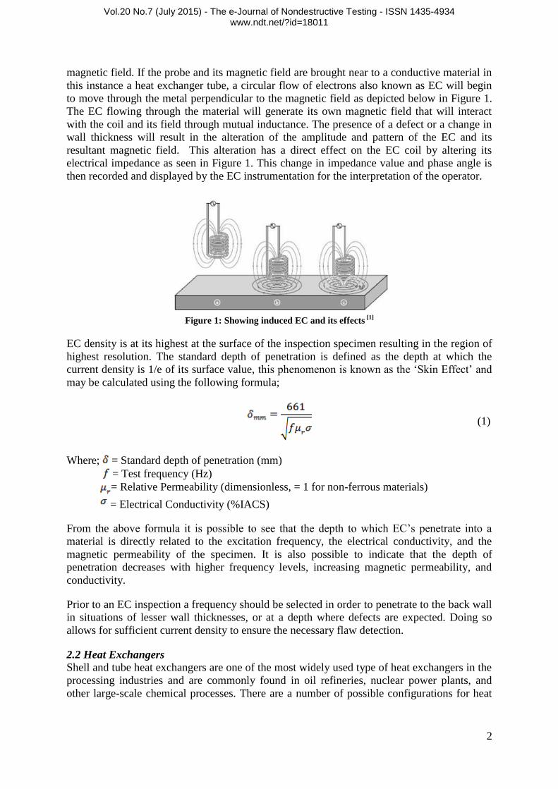
exchangers, but their basic concept can be shown with the description of some key

components. An example of a typical shell and tube heat exchanger is shown in Figure 2.

Figure 2: Showing a typical shell and tube type heat exchanger

[2]

From Figure 2 it is possible to see that heat exchangers operate by transferring heat from one

median to another. From the above example ‘Hot Air’ would enter through the ‘Air Inlet’ that

then flows through the heat exchanger in a rotational manner. This rotational flow of the air is

forced by the heat exchangers cylindrical geometry and its baffle plates. This allows for

circulation through the full heat exchanger increasing the path length resulting in increased

levels of heat transfer. Water is pumped to the ‘Water Inlet Tubes’ through the heat exchanger

allowing heat transfer between the ‘Hot Air’ and the ‘Water’ to take place.

Due to the moisture levels within the heat exchanger caused from both the internal flowing

water and the condensing air on the outer diameter of the tubes, it is clear that the oxidisation

of the tubes is inevitable resulting in wall ruptures and leaking tubes. This can cause major

disruptions in chemical plants forcing decommission until this problem is rectified.

2.3 Eddy current examination method

This method employs a probe (bobbin type) that contains one or more alternating current

(AC) coils that induce an electric field in the tube as previously stated in section 2.1. Prior to

the inspection process it is necessary that the EC system has been calibrated on a reference

standard with known, machined discontinuities, an example of this may be seen in Figure 3.

The probe is usually fired down the inspection tube and drawn back using an electric motor

machine at a constant speed; changes in coil impedance are recorded. The data may then be

displayed on a screen for data analysis and evaluation. Phase analysis and signal amplitude

are utilised to assess the depth, origin and size of flaws [3]

.

2.3.1 Advantages

Inspection speed up to approximately 60 feet per minute

Can detect gradual wall thinning and localised flaws

Provides both phase and amplitude information

Permanent records can be obtained on test results

By using multi-frequency techniques, flaws under the support plates (baffles) can be

found and evaluated accurately


4

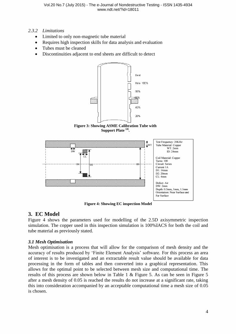
2.3.2 Limitations

Limited to only non-magnetic tube material

Requires high inspection skills for data analysis and evaluation

Tubes must be cleaned

Discontinuities adjacent to end sheets are difficult to detect

Figure 3: Showing ASME Calibration Tube with

Support Plate [4]

.

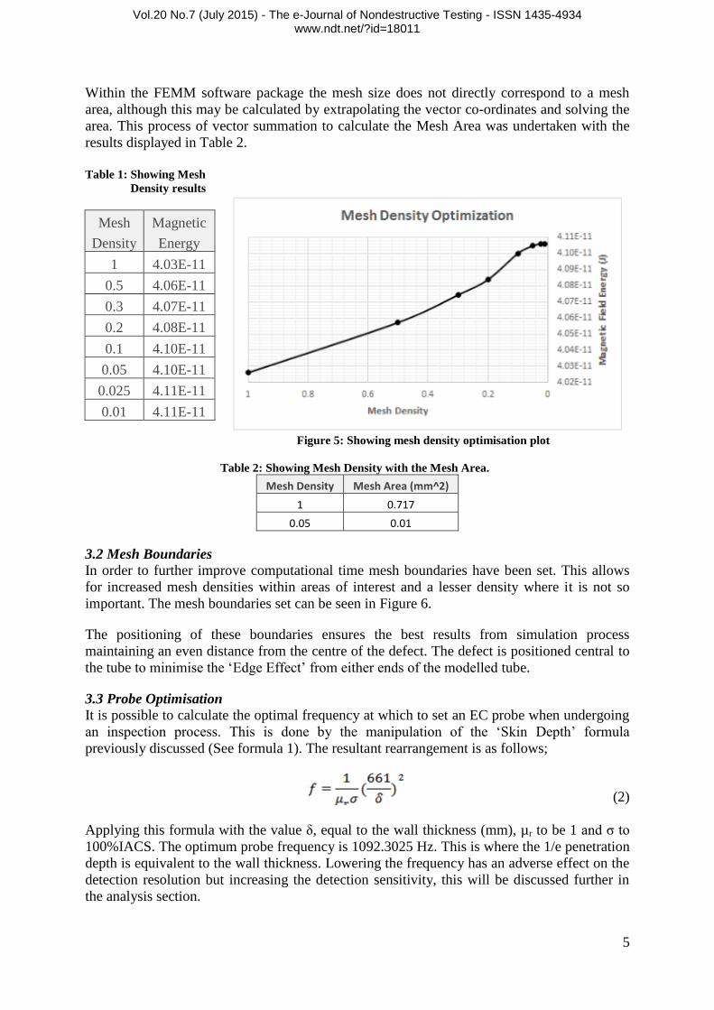
Figure 4: Showing EC inspection Model

3. EC Model Figure 4 shows the parameters used for modelling of the 2.5D axisymmetric inspection

simulation. The copper used in this inspection simulation is 100%IACS for both the coil and

tube material as previously stated.

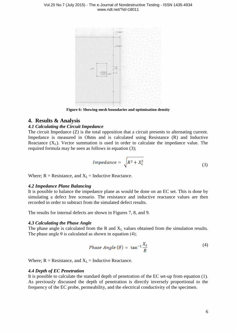
3.1 Mesh Optimisation

Mesh optimisation is a process that will allow for the comparison of mesh density and the

accuracy of results produced by ‘Finite Element Analysis’ software. For this process an area

of interest is to be investigated and an extractable result value should be available for data

processing in the form of tables and then converted into a graphical representation. This

allows for the optimal point to be selected between mesh size and computational time. The

results of this process are shown below in Table 1 & Figure 5. As can be seen in Figure 5

after a mesh density of 0.05 is reached the results do not increase at a significant rate, taking

this into consideration accompanied by an acceptable computational time a mesh size of 0.05

is chosen.


5

Within the FEMM software package the mesh size does not directly correspond to a mesh

area, although this may be calculated by extrapolating the vector co-ordinates and solving the

area. This process of vector summation to calculate the Mesh Area was undertaken with the

results displayed in Table 2.

Table 1: Showing Mesh

Density results

Figure 5: Showing mesh density optimisation plot

Table 2: Showing Mesh Density with the Mesh Area.

Mesh Density Mesh Area (mm^2)

1 0.717

0.05 0.01

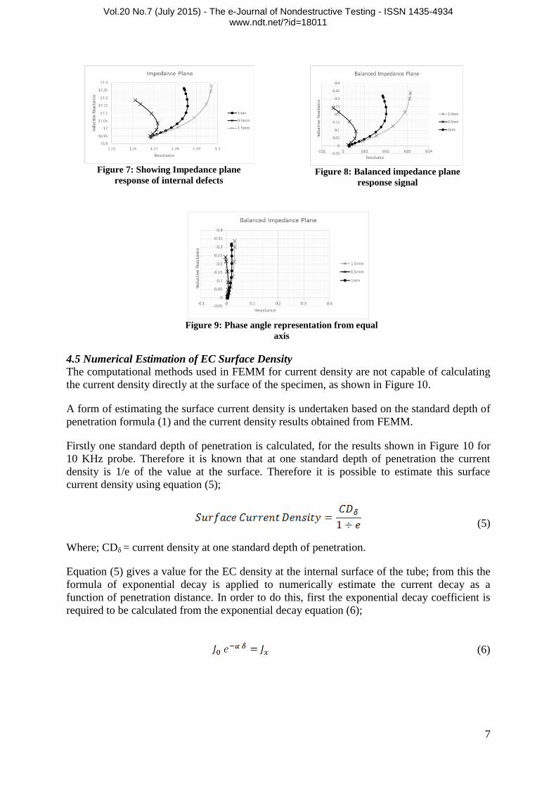
3.2 Mesh Boundaries

In order to further improve computational time mesh boundaries have been set. This allows

for increased mesh densities within areas of interest and a lesser density where it is not so

important. The mesh boundaries set can be seen in Figure 6.

The positioning of these boundaries ensures the best results from simulation process

maintaining an even distance from the centre of the defect. The defect is positioned central to

the tube to minimise the ‘Edge Effect’ from either ends of the modelled tube.

3.3 Probe Optimisation

It is possible to calculate the optimal frequency at which to set an EC probe when undergoing

an inspection process. This is done by the manipulation of the ‘Skin Depth’ formula

previously discussed (See formula 1). The resultant rearrangement is as follows;

(2)

Applying this formula with the value δ, equal to the wall thickness (mm), µr to be 1 and σ to

100%IACS. The optimum probe frequency is 1092.3025 Hz. This is where the 1/e penetration

depth is equivalent to the wall thickness. Lowering the frequency has an adverse effect on the

detection resolution but increasing the detection sensitivity, this will be discussed further in

the analysis section.

Mesh

Density

Magnetic

Energy

1 4.03E-11

0.5 4.06E-11

0.3 4.07E-11

0.2 4.08E-11

0.1 4.10E-11

0.05 4.10E-11

0.025 4.11E-11

0.01 4.11E-11


6

Figure 6: Showing mesh boundaries and optimisation density

4. Results & Analysis 4.1 Calculating the Circuit Impedance

The circuit Impedance (Z) is the total opposition that a circuit presents to alternating current.

Impedance is measured in Ohms and is calculated using Resistance (R) and Inductive

Reactance (XL). Vector summation is used in order to calculate the impedance value. The

required formula may be seen as follows in equation (3);

(3)

Where; R = Resistance, and XL = Inductive Reactance.

4.2 Impedance Plane Balancing

It is possible to balance the impedance plane as would be done on an EC set. This is done by

simulating a defect free scenario. The resistance and inductive reactance values are then

recorded in order to subtract from the simulated defect results.

The results for internal defects are shown in Figures 7, 8, and 9.

4.3 Calculating the Phase Angle

The phase angle is calculated from the R and XL values obtained from the simulation results.

The phase angle θ is calculated as shown in equation (4);

(4)

Where; R = Resistance, and XL = Inductive Reactance.

4.4 Depth of EC Penetration

It is possible to calculate the standard depth of penetration of the EC set-up from equation (1).

As previously discussed the depth of penetration is directly inversely proportional to the

frequency of the EC probe, permeability, and the electrical conductivity of the specimen.


7

Figure 7: Showing Impedance plane

response of internal defects

Figure 8: Balanced impedance plane

response signal

Figure 9: Phase angle representation from equal

axis

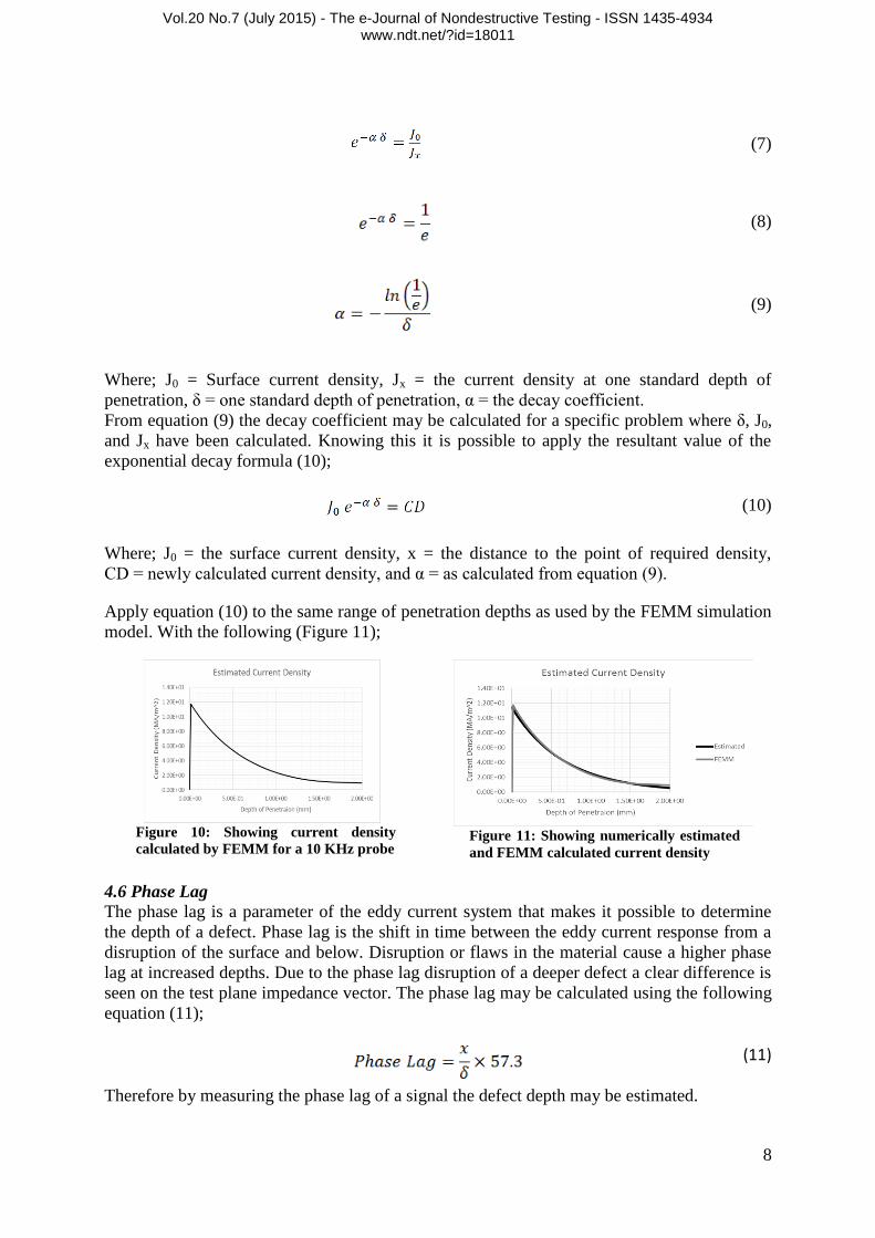
4.5 Numerical Estimation of EC Surface Density

The computational methods used in FEMM for current density are not capable of calculating

the current density directly at the surface of the specimen, as shown in Figure 10.

A form of estimating the surface current density is undertaken based on the standard depth of

penetration formula (1) and the current density results obtained from FEMM.

Firstly one standard depth of penetration is calculated, for the results shown in Figure 10 for

10 KHz probe. Therefore it is known that at one standard depth of penetration the current

density is 1/e of the value at the surface. Therefore it is possible to estimate this surface

current density using equation (5);

(5)

Where; CDδ = current density at one standard depth of penetration.

Equation (5) gives a value for the EC density at the internal surface of the tube; from this the

formula of exponential decay is applied to numerically estimate the current decay as a

function of penetration distance. In order to do this, first the exponential decay coefficient is

required to be calculated from the exponential decay equation (6);

(6)


8

(7)

(8)

(9)

Where; J0 = Surface current density, Jx = the current density at one standard depth of

penetration, δ = one standard depth of penetration, α = the decay coefficient.

From equation (9) the decay coefficient may be calculated for a specific problem where δ, J0,

and Jx have been calculated. Knowing this it is possible to apply the resultant value of the

exponential decay formula (10);

(10)

Where; J0 = the surface current density, x = the distance to the point of required density,

CD = newly calculated current density, and α = as calculated from equation (9).

Apply equation (10) to the same range of penetration depths as used by the FEMM simulation

model. With the following (Figure 11);

Figure 10: Showing current density

calculated by FEMM for a 10 KHz probe

Figure 11: Showing numerically estimated

and FEMM calculated current density

4.6 Phase Lag

The phase lag is a parameter of the eddy current system that makes it possible to determine

the depth of a defect. Phase lag is the shift in time between the eddy current response from a

disruption of the surface and below. Disruption or flaws in the material cause a higher phase

lag at increased depths. Due to the phase lag disruption of a deeper defect a clear difference is

seen on the test plane impedance vector. The phase lag may be calculated using the following

equation (11);

(11)

Therefore by measuring the phase lag of a signal the defect depth may be estimated.


9

(12)

Where; θ = phase angle, δ = one standard depth of penetration, and x = defect depth.

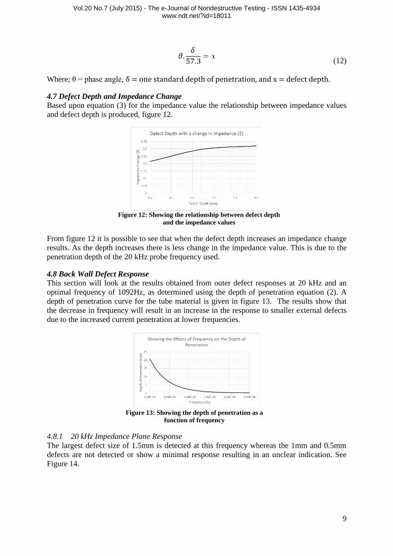
4.7 Defect Depth and Impedance Change

Based upon equation (3) for the impedance value the relationship between impedance values

and defect depth is produced, figure 12.

Figure 12: Showing the relationship between defect depth

and the impedance values

From figure 12 it is possible to see that when the defect depth increases an impedance change

results. As the depth increases there is less change in the impedance value. This is due to the

penetration depth of the 20 kHz probe frequency used.

4.8 Back Wall Defect Response

This section will look at the results obtained from outer defect responses at 20 kHz and an

optimal frequency of 1092Hz, as determined using the depth of penetration equation (2). A

depth of penetration curve for the tube material is given in figure 13. The results show that

the decrease in frequency will result in an increase in the response to smaller external defects

due to the increased current penetration at lower frequencies.

Figure 13: Showing the depth of penetration as a

function of frequency

4.8.1 20 kHz Impedance Plane Response

The largest defect size of 1.5mm is detected at this frequency whereas the 1mm and 0.5mm

defects are not detected or show a minimal response resulting in an unclear indication. See

Figure 14.


10

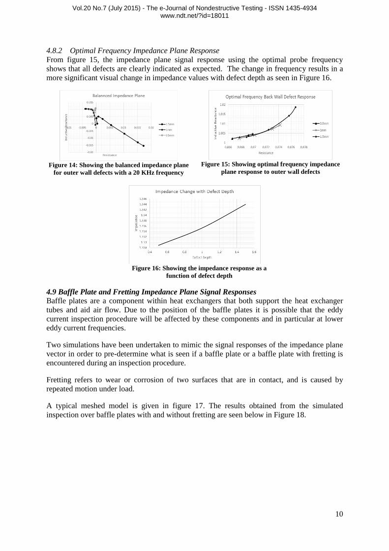
4.8.2 Optimal Frequency Impedance Plane Response

From figure 15, the impedance plane signal response using the optimal probe frequency

shows that all defects are clearly indicated as expected. The change in frequency results in a

more significant visual change in impedance values with defect depth as seen in Figure 16.

Figure 14: Showing the balanced impedance plane

for outer wall defects with a 20 KHz frequency

Figure 15: Showing optimal frequency impedance

plane response to outer wall defects

Figure 16: Showing the impedance response as a

function of defect depth

4.9 Baffle Plate and Fretting Impedance Plane Signal Responses

Baffle plates are a component within heat exchangers that both support the heat exchanger

tubes and aid air flow. Due to the position of the baffle plates it is possible that the eddy

current inspection procedure will be affected by these components and in particular at lower

eddy current frequencies.

Two simulations have been undertaken to mimic the signal responses of the impedance plane

vector in order to pre-determine what is seen if a baffle plate or a baffle plate with fretting is

encountered during an inspection procedure.

Fretting refers to wear or corrosion of two surfaces that are in contact, and is caused by

repeated motion under load.

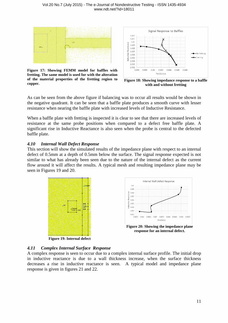
A typical meshed model is given in figure 17. The results obtained from the simulated

inspection over baffle plates with and without fretting are seen below in Figure 18.


11

Figure 17: Showing FEMM model for baffles with

fretting. The same model is used for with the alteration

of the material properties of the fretting region to

copper.

Figure 18: Showing impedance response to a baffle

with and without fretting

As can be seen from the above figure if balancing was to occur all results would be shown in

the negative quadrant. It can be seen that a baffle plate produces a smooth curve with lesser

resistance when nearing the baffle plate with increased levels of Inductive Resistance.

When a baffle plate with fretting is inspected it is clear to see that there are increased levels of

resistance at the same probe positions when compared to a defect free baffle plate. A

significant rise in Inductive Reactance is also seen when the probe is central to the defected

baffle plate.

4.10 Internal Wall Defect Response

This section will show the simulated results of the impedance plane with respect to an internal

defect of 0.5mm at a depth of 0.5mm below the surface. The signal response expected is not

similar to what has already been seen due to the nature of the internal defect as the current

flow around it will affect the results. A typical mesh and resulting impedance plane may be

seen in Figures 19 and 20.

Figure 19: Internal defect

Figure 20: Showing the impedance plane

response for an internal defect.

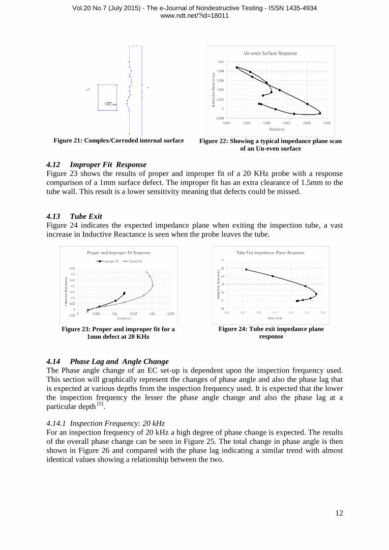
4.11 Complex Internal Surface Response

A complex response is seen to occur due to a complex internal surface profile. The initial drop

in inductive reactance is due to a wall thickness increase, when the surface thickness

decreases a rise in inductive reactance is seen. A typical model and impedance plane

response is given in figures 21 and 22.


12

Figure 21: Complex/Corroded internal surface

Figure 22: Showing a typical impedance plane scan

of an Un-even surface

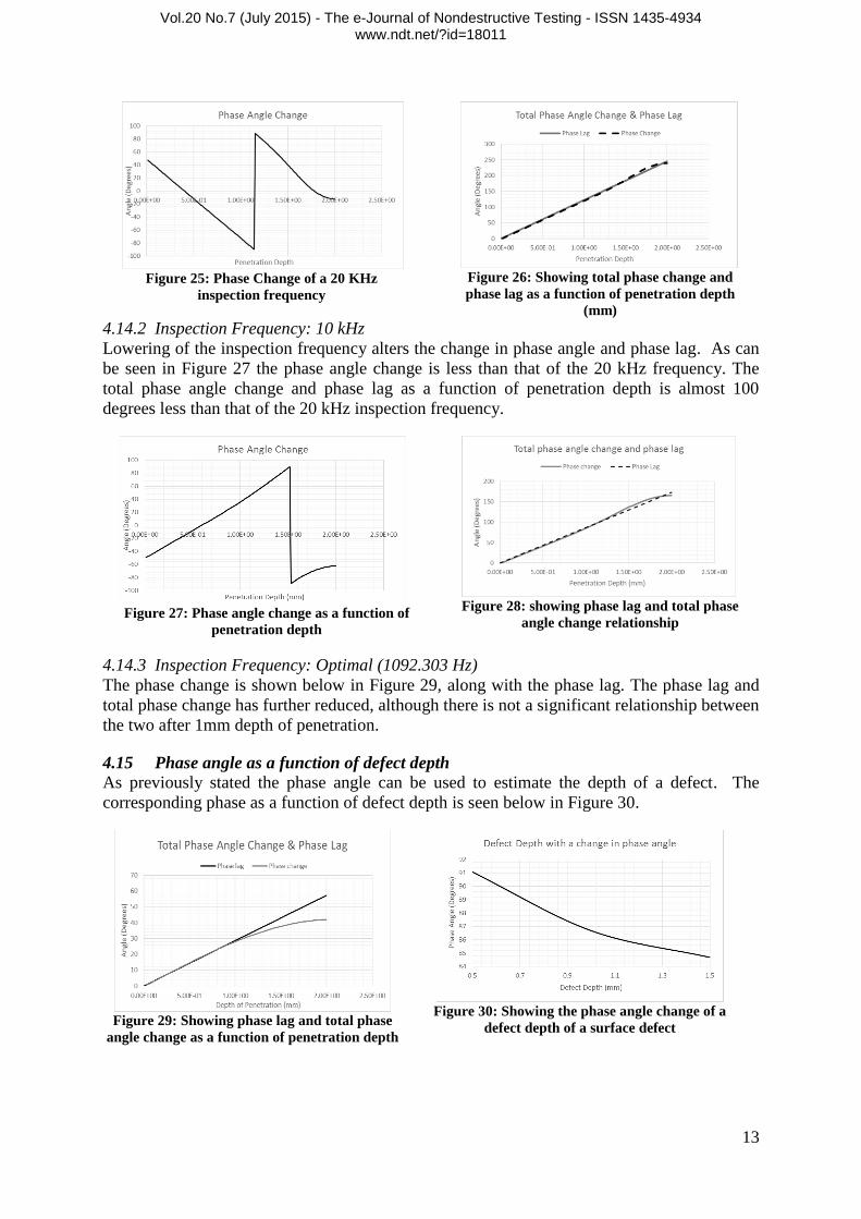
4.12 Improper Fit Response

Figure 23 shows the results of proper and improper fit of a 20 KHz probe with a response

comparison of a 1mm surface defect. The improper fit has an extra clearance of 1.5mm to the

tube wall. This result is a lower sensitivity meaning that defects could be missed.

4.13 Tube Exit

Figure 24 indicates the expected impedance plane when exiting the inspection tube, a vast

increase in Inductive Reactance is seen when the probe leaves the tube.

Figure 23: Proper and improper fit for a

1mm defect at 20 KHz

Figure 24: Tube exit impedance plane

response

4.14 Phase Lag and Angle Change

The Phase angle change of an EC set-up is dependent upon the inspection frequency used.

This section will graphically represent the changes of phase angle and also the phase lag that

is expected at various depths from the inspection frequency used. It is expected that the lower

the inspection frequency the lesser the phase angle change and also the phase lag at a

particular depth [5]

.

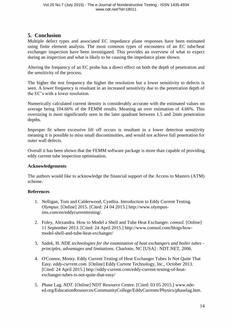
4.14.1 Inspection Frequency: 20 kHz

For an inspection frequency of 20 kHz a high degree of phase change is expected. The results

of the overall phase change can be seen in Figure 25. The total change in phase angle is then

shown in Figure 26 and compared with the phase lag indicating a similar trend with almost

identical values showing a relationship between the two.


13

Figure 25: Phase Change of a 20 KHz

inspection frequency

Figure 26: Showing total phase change and

phase lag as a function of penetration depth

(mm)

4.14.2 Inspection Frequency: 10 kHz

Lowering of the inspection frequency alters the change in phase angle and phase lag. As can

be seen in Figure 27 the phase angle change is less than that of the 20 kHz frequency. The

total phase angle change and phase lag as a function of penetration depth is almost 100

degrees less than that of the 20 kHz inspection frequency.

Figure 27: Phase angle change as a function of

penetration depth

Figure 28: showing phase lag and total phase

angle change relationship

4.14.3 Inspection Frequency: Optimal (1092.303 Hz)

The phase change is shown below in Figure 29, along with the phase lag. The phase lag and

total phase change has further reduced, although there is not a significant relationship between

the two after 1mm depth of penetration.

4.15 Phase angle as a function of defect depth

As previously stated the phase angle can be used to estimate the depth of a defect. The

corresponding phase as a function of defect depth is seen below in Figure 30.

Figure 29: Showing phase lag and total phase

angle change as a function of penetration depth

Figure 30: Showing the phase angle change of a

defect depth of a surface defect


14

5. Conclusion Multiple defect types and associated EC impedance plane responses have been estimated

using finite element analysis. The most common types of encounters of an EC tube/heat

exchanger inspection have been investigated. This provides an overview of what to expect

during an inspection and what is likely to be causing the impedance plane shown.

Altering the frequency of an EC probe has a direct effect on both the depth of penetration and

the sensitivity of the process.

The higher the test frequency the higher the resolution but a lower sensitivity to defects is

seen. A lower frequency is resultant in an increased sensitivity due to the penetration depth of

the EC’s with a lower resolution.

Numerically calculated current density is considerably accurate with the estimated values on

average being 104.66% of the FEMM results. Meaning an over estimation of 4.66%. This

oversizing is most significantly seen in the later quadrant between 1.5 and 2mm penetration

depths.

Improper fit where excessive lift off occurs is resultant in a lower detection sensitivity

meaning it is possible to miss small discontinuities, and would not achieve full penetration for

outer wall defects.

Overall it has been shown that the FEMM software package is more than capable of providing

eddy current tube inspection optimisation.

Acknowledgements

The authors would like to acknowledge the financial support of the Access to Masters (ATM)

scheme.

References

1. Nelligan, Tom and Calderwood, Cynthia. Introduction to Eddy Current Testing.

Olympus. [Online] 2015. [Cited: 24 04 2015.] http://www.olympus-

ims.com/en/eddycurrenttesting/.

2. Foley, Alexandra. How to Model a Shell and Tube Heat Exchanger. comsol. [Online]

11 September 2013. [Cited: 24 April 2015.] http://www.comsol.com/blogs/how-

model-shell-and-tube-heat-exchanger/

3. Sadek, H. NDE technologies for the examination of heat exchangers and boiler tubes -

principles, advantages and limitations. Charlotte, NC [USA] : NDT.NET, 2006.

4. O'Connor, Monty. Eddy Current Testing of Heat Exchanger Tubes Is Not Quite That

Easy. eddy-current.com. [Online] Eddy Current Technology, Inc., October 2013.

[Cited: 24 April 2015.] http://eddy-current.com/eddy-current-testing-of-heat-

exchanger-tubes-is-not-quite-that-easy/

5. Phase Lag. NDT. [Online] NDT Resource Centre. [Cited: 03 05 2015.] www.nde-

ed.org/EducationResources/CommunityCollege/EddyCurrents/Physics/phaselag.htm.

Documents

2.5D Finite Element Simulation Eddy Current Heat …repository.uwtsd.ac.uk/683/1/Pullen, A. and Charlton, P. (2015) 2... · 2.5D Finite Element Simulation – Eddy Current Heat Exchanger