SOCIIZIl?YOF PETROLEUMENGINEERS OF AIME PAPER

6200 North Central Expressway...-— enrUUM5M or L ~~~~

n=ll-. T.v. c ~~~gu._l_&O,” , ..*a”

THIS IS A PREPKUW --- SUBJECT TO CORRECTION

Steady-State Analysis of Gas Production,Transmission and Distribution Systems

By

Michael A. Stoner, ConsumersPower Co.

@ Copyright 1969American Institute of ,Mining, Metallurgical, and Petroleum Engineers, Inc.

This paper was prepared for the bbth Annual Fell Meeting of the Society of Petroleum Engineersof AIME2 to be held in Denver? C010.2 Sept. 28-Ott. 11 1969. Permissionto copy is restrictedto anabstract of not more than 300 words. Illustrationsmay not be copied. The abstract should containconspicuousacknowledgmentof where end by whom the paper is presented. I%blicationelsewhereafterpublication in the JOURNAL OF PETROLEUM TECHNOLOGYor the SOCIETY OF PETROLEUM ENGINEERS J(JJRNALisusually granted upon request to the Editor of the appropriatejournalprovided agreementto giveproper credit is made.

Discussion of this paper is invited. Three copies of any discussionshould be sent to theSociety of Petroleum Engineersoffice. Such discussionmay be presented at the above meeting and,v++h +ha manaw m.., ~~ nmnc.iAc.vaA Pnv n,.hl ~ nn+<nm. +m nma *P ~~,~ ~.wt~ ~~~ .nerr.e<nnc.7A”.. “L.* .&9PLA 3 ‘LA-J ~-~’-J-=~’~= ‘VJ’ .tJuw~~’-’=u~uL~ ~~~ u~~= -~ ,LLct.~a L, J.,,’G a .

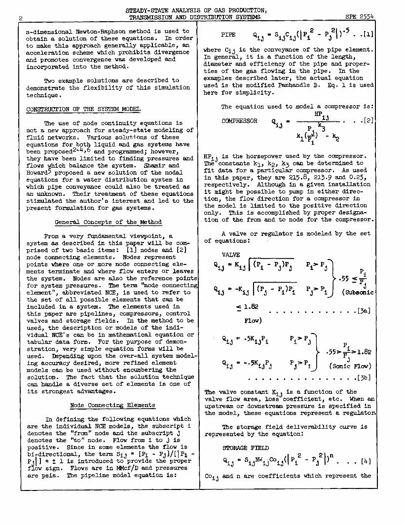
ABSTRACT First, the method can be used to simulate anintegrated system composed of aii the elements

This paper presents a new method for found in a gas system [i.e.,pipelines, compres-obtaining a steady-statesolution of an inte- aors, control valves, production fields andgrated gas system model made up of pipelines, peak shaving elements such as storage fields andcompressors,control valves and storage fields. ING plants]. This systems’ analysis approach toBy use of this very flexible solution techuique, modeling gas systems allows the designer toit is possible to solve directly for systemfacility parameterswhen pressure and flow

perform a much more comprehensivestudy thanwith previous methods. With this model the

specificationshave been given. The mathemati- designer can measure the interactionof anycal model of a system consists of node conti.n- system componentall in the sme simulationuity equationswhich are solved by the n- progran. Second, to the author’s knowledge,dimensionalNewton-Raphsonmethod. published network analysismethods have been

restrictedto determiningsystem pressures andINTRODUCTION flows. By treating the equationswhich repre-

sent the model in a very general way, it isNatural gas systems are becoming more and possible to include system element parameters

more complex as the use of this energy source other than pressure and flow as unknowns.4“..-.”-. Iln..-1...->---4 &l..!- -.—-1 ,...-?4... . . ...-4. ---- —.-- L–.. – -r, *.-. . . . . .. . . . . . . . . –– —. -.. >.- —– *-..ALLLAcancD . LUC UIALUCU UL blJLb UJIIl&JLCALL.y IU(.tbb raramezers 01 zne moae~ sucn as pipe amme~er,be borne by the persons responsiblefor the compressionhorsepower,valve settings anddesign and operation of these aystema. Mathe- number of storage field wells can be determinedmatical modeling is one of the more important when appropriatepressure and flow specifica-tools used to aid in design and operation t.ion~are mafle, This featu_reis Qf areatstudies. The systems under consideration

~--—.,importanceto the system designer, since system

actually operate in an unsteady nature, and parameters can be obtained directly instead of~~~~-ouahmuch ~ffQ.ti:~MS ~~~~ a~~ CQ~~.i~U~S@_. —---- r7a+nminimu ~~Ae~~y +.Pin7-snA-nvv.nv mFn.eA,,ma.q. ...u.u...~

be spent on unsteady mathematicalmodels, many“--— —- ---”- .F?~-----~~-*

design problems can amd wiU be solved by The model proposed in this paper is con-steady-statemodeling. It is, therefore, struttedby writing the continuityequation atdesirableto extend the steady-statemodeling each node in the system. The flow equation forcapabilitiesto accommodatethese complex sys- each element connectedto the node is thenternsin their entirety. This paper presents a substitutedto eliminate the element flow. Thissteady-statemodel and one solution technique results in a set of nonlinear simultaneousequa-for this model which has two important features. tions which constitutethe system model. TheReferences and illustrationsat end of paper.

STEADY-STATE ANALYSIS OF GAS PRODUCTION,2 TRANSMISSIONAND D]

n-dimensionalNewton-Raphsonmethod is used toobtain a solution of these equations. In orderto make this approach generally applicable,anacceleration scheme which prohibits divergenceand promotes convergencewas developed andincorporatedinto the method.

Two exsmple solutions are described to.. L—-A AL. S1 “4k414+., a+ +hi= ~~lfl~~.~on

ckrnonssrube U= LL2LLUAL..J -. -.&u

technique.

CONSTRUCTIONOF THE SYSTEM MODEL

The use of node continuityequations isnot a new approach for steady-statemodeling off’l,,iaTle+l.Tn7kc!.AUAU SU..”...”● ~~~i~l~~~QIutiQns of theseequations for both liquid and gas systems havebeen proposed2-4~6and programmed; however,they have been limited to finding pressures andflows which balance the system. Shamir andHoward~ proposed a new solution of the nodalequations for a water distributionsystem inwhich pipe conveyance could also be treated asan unknown. Their treatment of these equationsstimulatedthe author’s interest and led to thepresent formulation for gas systems.

General Concepts of the Method

From a very fundamentalviewpoint, asystem as described in this paper will be com-prised of two basic items: [I] nodes and [2]node connectingelements. Nodes representpoints where one or more node connectingele-ments terminate and where flow enters or leavesthe system. Nodes are also the referencepointlfor system pressures. The term “node connectin{element”, abbreviatedNCE, is used to refer tothe set of all possible elements that can beincluded in a system. The elements used inthis paper are pipelines; compressors,controlvalves and storage fields. ~ the method to beused, the descriptionor models of the indi-vidual NC!E’Scan be in mathematical equation ortabular data form. For the purpose of demon-stration, very simple equation forms will beused. Depending upon the over-all system model.ing accuracy desired, more refined elementmodels can be used without encumberingthesolution. The fact that the solution techniquecan handle a diverse set of elements is one ofits strongest advantages.

Node ConnectingElements

In defining the following equationswhichare the individual NCE models, the subscript idenotes the “from” node and the subscript jdenotes the “to” node. Flow from i to j ispositive. Since in some elements the flow ishi-directional,the term Sij ‘ [Pi - Pj]/[lPi -Pull = t 1 is introducedto provide the properfiow sign. Flows are in MMcf/D and pressuresare psia. The pipeline model equation is:

!RIBUTION SYSTEMS - SPE 2554

PIPE Q. =sifij(pi2 - P#21)”5 “ “[dlJ

where Cij is the conveyanceof the pipe element.In general, it is a function of the length,dismeter and efficiency of the pipe and proper-ties of the gas flowing in the pipe. In theexamples described later, the actual equationused is the modified Panhandle B. Eq. 1 is usedhere for simplicity.

The equation used to

~~~~~~~Qij =

model a compressoris:

‘ij r2]~ k= ● “ “’

k,(j) ‘- k2--

i

Hpij iS the horsepower used by the compressor.The constantskl, k2, k3 can be determinedtofit data for a particular compressor. As usedin this paper, they are 215.8, 213.9 ~d o.25~respectively. Although in a given installationit might be possible to pump in either direc-tion, the flow direction for a compressorinthe model is limited to the positive directiononly. This is accomplishedby proper designa-tion of the from and to node for the compressor.

A valve or regulator is modeled by the setof equations:

VALVE

QU”KW-7T ‘,”’, pi

Qij }‘-%IF=E ‘j”pi“:62<1.82.............[*I

F1ow)

Qij=“5Kijpi‘i>p

}

3 ‘i.55>FS1.82

‘ij = -“%jpj P >Pi$ (Soni: Flow)

. . . . . . . . . . . ..0. .[3b]

The valve constant ~j is a function of thevalve flow area, loss coefficient>etc. When aIupstream or downstreampressure is specified inthe model, these equations represent a regulatol

The storage field deliverabilitycurve isrepresentedby the equation:

STORAGE FIELD

*J = SijNtiijCoij(lPi2- Pj21)no .Q. . [4]

Coij and n are coefficientswhich representthe

iPE2554 MICHAEL

production capabilitiesof one well. Nwi isithe number of wells in the field. For th s

element, one node representsthe wellhead,while the other node references an imaginarypoint in the reservoirthrough which all flowenters and leaves the field. The pressure atthis point is the field pressure and can berelated to the field inventoryby use of thefield pressure-volumerelationship. In thispaper, n = 0.69.

These equations represent the mathematicalmodel for each componenttype that will.beincluded in the total system. The next step isto assemble these componentsin such a way thata complete system model is obtained.

Node ContinuityEquations

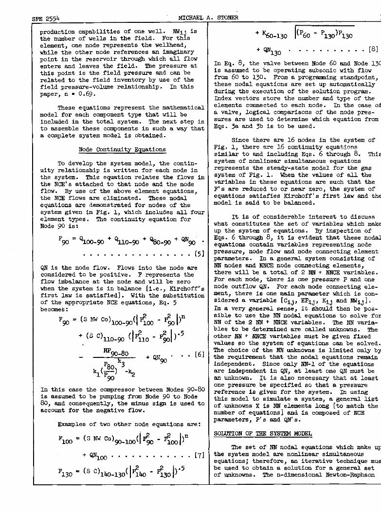
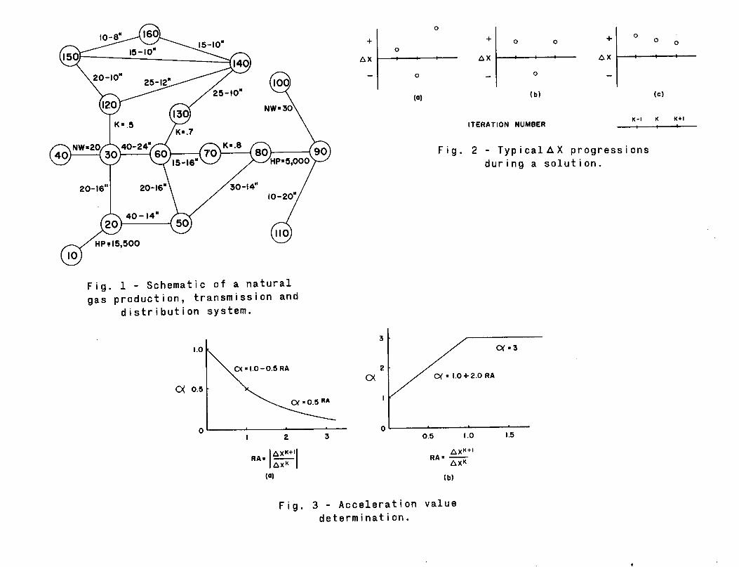
To develop the system model, the contin-uity relationshipis written for each node inthe system. This equation relates the flows inthe NCE’S attached to that node and the nodeflow. By use of the above element equations,the NCE flows are eliminated. These nodaleauations are demonstratedfor nodes of the->—..system given in Fig. 1, which includes all fouxelement types. The continuityequation forNode 90 is:

L)(3=%0+0 +Qllo.go”+ Q&)-go+ QNgo ●

● ✎ ✎ ✎ ✎ ✎ ✎ ✎ ✎ ✎ ✎ ✎ ✎ ✎ ✎ ✎ [51

QN is the node flow. Flows into the node areconsideredto be positive. F representstheflow imbalanceat the node and will be zerowhen the system is in balance [i.e.,Ktrchoff’”sfirst law is satisfied]. With the substitutionof the appropriateNCE equations,Eq. 5becomes:

‘90-80 +QN”” . [6]

’80 ‘390

k,(~) -~-. —

In this case the compressorbetween Nodes 90-80is assumed to be pumping frcnnNode 90 to Node80, and consequently,the minus sign is used toaccount for the negative flow.

Examples of two other node equations are:

‘loo if - <ml)”= (sNdCo)W-l~( 90

‘Q%OO” “ “ “ “ “ “ “ “ “ “ “ [71

F130 = (S C) IW-130( 1<40- <301)”5

. STONER

+ %0-130 ~-

‘%30 “ “ “ “ “ ““ “ ● “. [8]

In Eq. 8, the valve between Node 60 and Node 130is assumed to be operating subsonicwith flowfrom 60 to 13o. From a programming standpoint,these nodal equations are set up automaticallyduring the execution of the solutionprogrsm.Index vectors store the number and type of theelements connectedto each node. In the case ofa valve, logical comparisonsof the node pres-sures are used to determinewhich equation fromEqs. 3a and 3b is to be used.

Since there are 16 nodes in the system of-> ‘t~~~.~v~ ~~ ~QEtiE1uqr equations~jge 7

similar to and includingEqs. 6 through 8. TkliS

system of nonlinear simultaneousequationsrepresents the steady-statemodel for the gassystem of Fig. 1. When the values of all thevariables in these equations are such that theF’s are reduced to or near zero, the system ofequations satisfiesfirchoff’s first law and themodel is said to be balanced.

~~ is of ~~~~id~~~~~~ i~~~~~~~ ~CIdisc~~swhat constitutesthe set of variableswhich makeup the system of equations. By inspectionofEqs. 6 through 8, it is evident that these nodalequations contain variables representingnodepressure, node flow and node connectingelementparameters. In a genersl system consisting ofNN nodes and NNCE node connectingelements,there will be a total of 2 NN + NNCE variables.For each node, there is one pressure P and onenode outflow QN. For each node connectingele-ment, there is one main parameter which is con-sidered a variable [Cij,HPij, Kij ~d NWij].

in Ei very general sense, it slm-uldthen be pos-sible to use the NN nodal equations to solve forNN of the 2 NN + NNCE variables. The NN varia-bles to be determinedare called unknowns. Theother NN + NNCE variablesmust be given fixedvalues so the system of equations can be solved.The choice of the NN unknowns is limited only bythe requirementthat the nodal equations remainindependent. Since only NN-1 of the equationsare independentin QN, at least one Q,Nmust be~ mow.

1% is Qs~ ~~~~ssaiiy- that Gt lmstone pressure be specified so that a pressurereference is given for the system. )22 usingthis model to simulate a system, a general listof.unknownsX is NN elements long [to match thenumber of equations] and is composed of NCEparameters, P’s and QN’s.

SOLUTION OF THE SYSTEM MODEL

The set of NNnodal equationswhich make upthe system model are nonlinear simultaneousequations;therefore, an iterativetechnique musbe used to obtain a solution for a general setof unknowns. The n-dimensionalNewton-Raphson

STEADY-STATEANALYSIS OF GAS PRODUCTION,4 TRANSMISSIONAND DISTRIBUTION SYSTEMS - SPE 2554

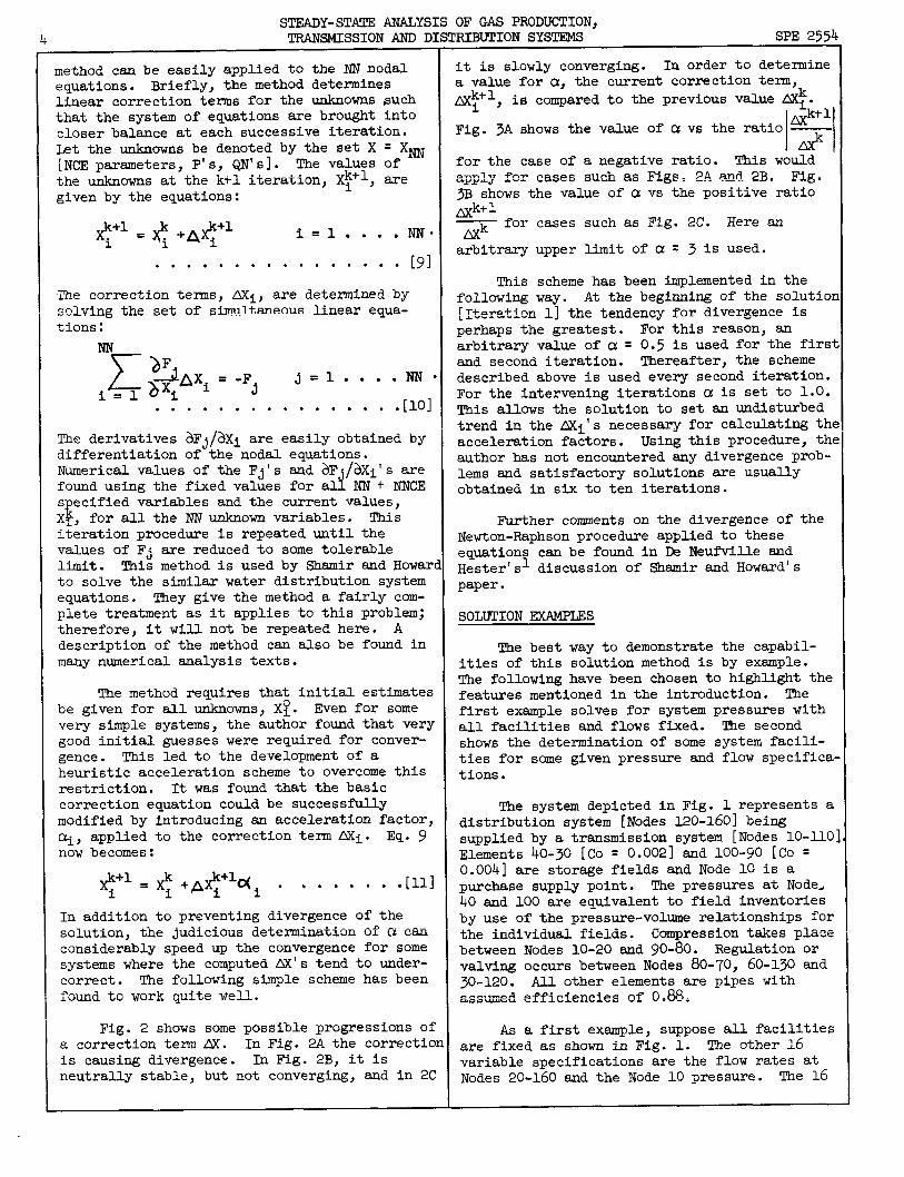
method can be easily applied to the NN nodalequations. Briefly, the method determineslinear correctionterms for the unknowns suchthat the system of equations are brought intocloser balance at each successive iteration.Let the unknowns be denoted by the set X = Xm[NCEparsmetersj P’s, w’s]. The v:ECL::Softhe unknowns at tinek+i iteration, A: -, Sz’e

given by the equations:

i =1 . . . .NN”

. . . . . . . . . . . . . . . . [91

The correctionterms, AXi, are determinedby~~~~i~g the set Qf simultaneous linear equa-tions:

NN

z >F-+i=-Fj J=l . . ..NN

i = 1 Wi. . . . . . . . . . . . . . . .[10]

The derivatives &Fj/3Xi are easily obtained bydifferentiationof the nodal equations.Numerical values of the Fj’s ~d ~F”/~Xi’S mefound using the fixed values for a~NN+NNCEs ecified variables and the current values,XE~, for all the NN unknown variables. Thisiterationprocedure is repeated until thevalues of Fj are reduced to some tolerablelimit. This method is used by Shsnir and Howarto solve the similar water distributionsystemequations. They give the method a fairly com-plete treatment as it applies to this problem;therefore, it will not be repeated here. Adescription of the method can also be found inmany numerical analysis texts.

The method requires that initial estimatesbe given for all unknowns, X!. Even fOr somevery simple systems, the author found that verygood initial guesses were required for conver-gence. This led to the developmentof aheuristic acceleration scheme to overcome thisrestriction. It was found that the basiccorrectionequation could be successfullymodified by introducingan accelerationfactor,~, applied to the correctionterm lSXi. Eq. 9now becomes:

xp=xJ’+&%i ● ● . . . . ..[11Ii

In addition to preventing divergence of thesolution,the judicious determinationof’rzcanconsiderablyspeed up the convergencefor somesystems where the computedAX’s tend to under-correct. The following simple scheme has been-f~~~ +“~7wr~~Jb>~di~~ .“T~a~●

Fig. 2 shows some possible progressionsofa correctionterm ZIX. In Fig. 2A the correcticis causing divergence. In Fig. 2B, it isneutrally stable, but not converging,and in 2C

it is slowly converging. In order to determinea value for a, the current correctiontern,~k+ 1

i) is compared to the previous value m!.&+l

Fig. 3A shows the value of a vs the ratio —d

for the case of a negative ratio. This would.TYP.l.r f~~ @,,cj~s ~luc~. ~S ~i~~: ~.A-~d ~B, _.=.‘~y‘J

FiQ

3B shows the value of a vs the positive ratio~k+ 1

~k for cases such as Fig. 2C. Here an

arbitrary upper limit of a = 3 is used.

This scheme has been hplemented in thefollowingway. At the beginning of the solutionr-r+GW9+.+nn71 ~~~ ~~~~~~qr for divergence iSLO--------- -Jperhaps the greatest. For this reason, ~arbitrary value of c%= 0.5 is used for the firstand second iteration. ~ereafter, the schemedescribed above is used every second iteration.For the interveningiterationsa is set to 1.0.This allows the solution to set an undisturbedtrend in the &i’s necessary for calculatingtheaccelerationfactors. Using this procedure, theauthor has not encounteredany divergenceprob-lems and satisfactorysolutionsare usuallyobtained in six to ten iterations.

Further comments on the divergence of theNewton-Raphsonprocedure applied to theseequations can be found in De Neufville andHester’sl discussionof Shamir and Howard’spaper.

SOLUTION EXAMPLES

The best way to demonstratethe capabil-ities of this solutionmethod is by exsznple.The followinghave been chosen to highlight thefeaturesmentioned in the introduction. Thefirst example solves for system pressureswithall facilitiesand flows fixed. The secondshows the determinationof some system facili-ties for some given pressure and flow specifica-tions.

The system depicted in Fig. 1 representsadistributionsystem [Nodes120-160]beingsuppliedby a transmissionsystem [Nodes1O-IJ-OElements 40-30 [Co = 0.002] and 100-90 [C!O=0.004] are storage fields and Node 10 is apurchase supply point. The pressures at Node.40 and 100 are equivalentto field inventoriesby use of the pressure-volLmIerelationshipsforthe individual.fields. Compressiont~es placebetween Nodes 10-20 and 90-80. Regulation orvalving occurs between Nodes 80-70,60-130and30-120. All other elements are pipes with.O.!l-l-an++-1”-lnn.iaeof 0,88,-Dmu.u .......-...”

As a first exsmple, suppose all facilitiesare fixed as shown in Fig. 1. The other 16variable specificationsare the flow rates atNodes 20-160 and the Node 10 pressure. The 16

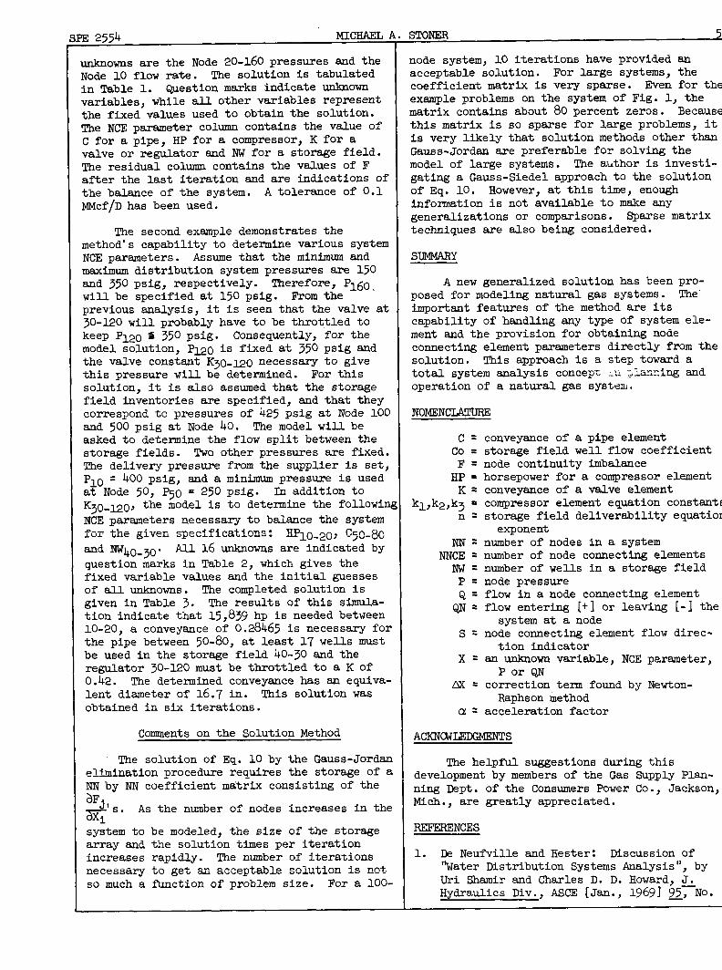
?E2554 MICHAEL P

unknowns are the Node 20-160 pressures and theNode 10 flow rate. The solution is tabulatedin Table 1. Questionmarks indicateunknownvariables,while all other variables representthe fixed values used to obtain the solution.The NCE parameter column contains the value ofC for a pipe, HP for a compressor,K for avalve or regulator and NW for a storage field.The residual column containsthe values of Fafter the last iterationand are indicationsofthe balance of the system. A tolerance of 0.1MMcf/Dhas been used.

The second example demonstratesthemethod’s capabilityto determine various systemNCE parameters. Assume that the mintium andmaximum distributionsystem pressures are 150and 350 psig, respectively. Therefore, P160will be specified at 150 psig. From theprevious analysis, it is seen that the valve at30-120 will probably have to be throttled tokeep P~O S 350 psig. Consequently,for themodel solution,P120 is fixed at 350 psig andthe valve constantK30-120 necessary to givethis pressure will be determined. For thissolution, it is also assumed that the storagefield inventoriesare specified,and that theycorrespondto pressures of 425 psig at Node 100and 500 psig at Node 40. The model will beasked to determine the flow split between thestorage fields. Two other pressures are fixed.The delivery pressure from the supplier is set,

%0 = 400 psig, and aminimun pressure is usedat Node 50, P50 = 250 psig. In addition to

K30-120~ the model is to determinethe followln{

NCE parameters necessary to balance the system--- *U- “<.. - c’nani++.=++nn~:LUL bLIC ~Lveu ~p=b~.~tiw.~u- . q~-+~; (@gj(j

ad ~40-30. All 16 unknowns are indicatedby

questionmarks in Table 2, which gives thefixed variable values and the initial guessesof all unknowns. The completed solution isgiven in Table 3. The results of this simula-tion indicate that 15,839 hp is needed between10-20, a conveyanceof 0.28465 is necessary forthe pipe between 50-80, at least 17 wells mustbe used in the storage field 40-30 and theregulator 30-120 must be throttled to a K of0.42. The determined conveyancehas an equiva-lent diameter of 16.7 in. ~is solutionwasobtained in six iterations.

Comments on the SolutionMethod

me solution of Eq. 10 by the Gauss-Jordaneliminationprocedure requires the storage of aNN by NN coefficientmatrix consistingof theaF

2‘s. As the number of nodes increases in the

xisystem to be modeled, the size of the storagearray and the solution times per iterationincreasesrapidly. The number of iterationsnecessary te get an ~LGePU-.A= s.A....-... .l+.lmla n17,+inn is ~Q~

so much a function of problem size. For a 100-

STONER c<

node system, 10 iterationshave provided anacceptable solution. For large systems, thecoefficientmatrix is very sparse. Even for th(exsmple problems on the system of Fig. 1, thematrix contains about 80 percent zeros. Becausfthis matrix is so sparse for large problems, itis very likely that solutionmethods other thanGauss-Jordanare preferable for solving themodel of large systems. The author is investi-gating a Gauss-Siedelapproach to the solutionof Eq. 10. However, at this time, enoughinformationis not availableto make anygeneralizationsor comparisons. Sparse matrixtechniques are also being considered.

SUMMARY

A new generalized solutionhas been pro-posed for modeling natural gas systems. The”important features of the method are itscapabilityof handling any type of system ele-ment and the provision for obtainingnodeconnectingelement parameters directly from thesolution. This approach is a step toward atotal system analysis concept LL planning andoperation of a natural gas system.

NOMENCLATURE

c=co =F=Hp .

K=

k1Jk2Jk3 ‘n=

NN=NNCE =NW=P==

$=

s=

x=

m=

a:

conveyanceof a pipe elementstorage field well flow coefficientnode continuityimbalancehorsepower for a compressorelementconveyanceof a valve elementcompressorelement equation constantstorage field deliverabilityequatioexponent

number of nodes in a systemnumber of node connectingelementsnumber of wells in a storage fieldnode pressureflow in a node connectingelementflow entering [+] or leaving [-] thesystem at a node

node connectingelement flow direc-tion indicator

an unknown variable, NCE parameter,PorQN

correctionterm found by Newton-Raphson method

accelerationfactor

AcKNUtrLEDGMENTS

The helpful suggestionsduring thisdevelopmentby members of the Gas Supply Plan-ning Dept. of the ConsumersPower Co., Jackson,Mich., are greatly appreciated.

REFERENCES

1. De Neufvilleand Hester: Mscussion of“Water DistributionSystems Analysis”,byUri Shamir and Charles D. D. Howard, J.Hydraulics Div., ASCE [Jan., 19691~7N0.

STEADY-STATE ANALYSIS OF GAS PRODUCTION,

HYl, 484-486.2. Hyman, S. 1.: “NetworkAnalysis by the

Method of Adjusting Pressures”,Faper GSTS-63-9 presented at AGA Operating SectionTransmissionConference [1963].

~, Marlow$ T. A.} Hardison, R. L., Jacobson>H. and BiggS, G. E.: “IinprovedDesign ofFluid Networkswith Computers”,J.@#j_rEuJMcs IMv.> ASCE [July> 19~92j No.

HY4, paper 4866, 43-61.4. McCoi’mick,M. and ~ll~y, C. J.: “A

Computer Program for the Analysis of Net-works of Pipes emd Pumps”, J.-InstitutionofEngineers, Australia [Muwh, 1968j Paper2419, 51-58.

5. Shamir, U. and Howard, C. D. D.: “WaterDistributionSystems Analysis”,~Hydraulics Div., ASCE [Jan., 19tij ~, No.HYl, 219-234.

6. Str~eter,V. L.: “Water-HemmerAralysis ofDistributionSystems”, J. Hydraulics Div.,ASCE [Sept.,19671 93, NO. HY5, 185-201.—

Table 1 - Summary of Example 1 solution.

NODE DATA

..-.——. — —..—..__- — . .

NODE PiE<;iURE FLCiIJ <ksIOU~L (F)

—— ..-——.———. —.—10 4U0.OC 396.0 ? -!).001720 763*26 ? coo 0.001”1>0 ;07.19 ? -350.0 U.0034 __60 306.!i’3? -200.0 -0.0UZ3Bn 434.50 ? o.@ -0.0013

- ia3.li ?<6 -1.0 O.ctlloLOJ 395686 ? ‘“3DC.O -0.0U02L10 Zb2.42 ? -100.0 -0.JuC47J 3~L.33 ? 0.0 0.0002 _.-.——————30 +28.02 ? -5C.C -0.00G240 508-74 ? 100.0 -0.00’21

_L 820 365.98 ? 0.0 -C*OO0213) 334.45 ? C.o -Ooi)GCIO140 246,42 ? –25.0 0.0001

_l.!)3 -35.!) O.OJ”)L _.227.95 ? _._-—.—.—.160 159s06 ? -40.0 O*OOOL

NCE DATA AND FLOWS

FROM TO

NODE NODETYPE FLOW NCE

PARAMETER

CtiMP 396.00 L550G.PIP-E- l_46.Lo._._...._b03.>3.>.L_..PIPE -109./!2 C.3Z!)51PIPE -93.’3ti (3.LS591cGv.? Lq>,l)l)-.. 5CC0.FIELD 3C)U.LJO 3j.()PIPt 100.00 o.tio~b~

RE.; . . LU5*%2... . . . ...U.60JOC.PIPC ~!:>eq;~ 3.?7116PIPE ~~~.~G 0.5275JPI?E .247.911 P.52051FIkL!l ‘“ itiii.(ii) 20.b

Rtb ~b. 34 CI.500GJ

..60 130...R_EG_ _...-139 L40 PIPEA20 140 PIPE 43.95 G.L331%

Tsble 2 - Fixed variable data and initial values

(f’) of the unknowns for Example 2.

FromN@_~

iO2050

2)100908070302040

2130120120140140150

Node

10205040

E

~90llo100320130140150160

ToNcde

m

i%

8

wI.lo7060603030

lx?o130140140

i%150160

(r&@ ~

PmPIPE ‘1cow

Pm

mmPIPEPmFIELO ?REG?REGPIPEPIPEPIPEPIPEPIPEPIPE

NODE INIWM4TION

Pressure

%: 7250.

%: ?400. ?500. 7510. ?200. ?150. ?425.3!W.350. 7250. ?2m. ?150.

NCEParemeter

~~&-)Q ~

.1605

.3205

.18595000.

.82J

7TI c1.>1=

.6278

.320520.

95

.08;

.1381

.0976● 1130.1130●W9

Flow

3S6.

-34:100. ?-50.-200.

o*o*i.

-loo*300. ?o.0.

- 25.~ %.

.

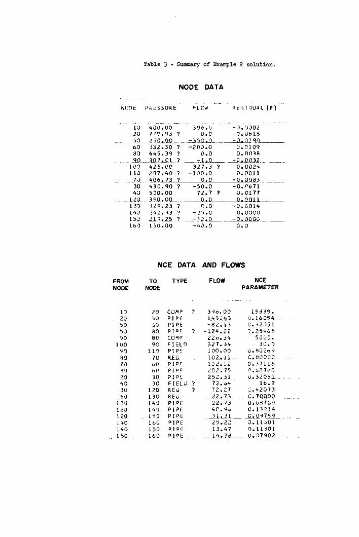
Table3 - Summaryof Example2 solution.

NODE DATA

.

iJl!r)t PIlissuRE PLC’# ‘“- RtS”liUAL (F) ““

. -.10 -430.00 --- 396.0 -J.”:)30i ““-‘“20 77q .93 ? O.c f20d61El

-—. ~g 2mdlll____..:2512,.9..__% ’22?.Q_____60 332.30 ? -20G. U 0.9109SQ ++fj=~q ? *o=() O 0038.s....

---.–..2QL–XJL!!l_3_ -1.0 ..—4J!Q32 .... —---]~~ 425.00 327.3 ? O* 0024110 .?87.40 ? -10000 C),@oll_._?J.. +Qb2_73 ? 0.0 -,-.. 0 m33-.._ .—.30 430.90 ? -50.0 -oop~7143 530.00 72-7 ? fJ*c177

–_..L2o..3.5.Q..oQ----___4~L—-----i39 j2Q.23 ? C*O -().G014L42 ?42. 33 ? -25*Q 0.0000150 d L 25. ? ...2$2..Q._ -_-.Sklwlo..-.—Lb’o 150.00 -4(!.!l G*O

NCE DATA AND FLOWS

To-. ---TYI-% FL(W tilerNkc

NODE PARAMETER

.— ..

20505Gso8(!9C

110----70b(.)5(!3030

12CJ13@14014(I1$59lb(l)150160

CON? ?PIPEPIPEplo~ ?cr.)$1~FItL~

P!p:RE&PIPE

PJ~:p~p:FIELLI ?REG ?R-EGPIPEPI?~

PIPEPIPEPIPE

P1OE

3+e. 00 1533Q*143* 5.3 Co16054..-82.13 C.”32:)51

-124.2Z :.294652,20.54 j~J~*

327.34 3~;.’3~~)~,~o <.f+(j~~q

1(22..11– C.i!i?oo.c .102. IZ c..i7llb292.75 1>.>27t<c252.31 - U..3LC’.51 ...

72.04 16s2-.!4. <?7 ;. 42073

.2.2.. .?3.. ..C.. 7.c.g.oo . _.22.73 i3. i)47ci Y4c.~0 ().13314

.__7.L..2L .— .-!2-1Q.+ 75-9_ . . ..- –25.22 0.1130113.47 0.11301

— Jkq.zB____Q.,3.7Q.(1?_ . ._

K=.5

Nwx20

20-16” 20-16”

/.--/HP ?15,500

v10

Fig. 1 - Schematic of a natural

gas proc!uct ion, transmission and

distribution system.

I .0 5

0(=1.O-O.5RA

a 0.5 “

~1

I 2 3

(a)

(a) (b) (c)

ITERATION NUMSERK-1 K K+l

Fig. 2 - Typical AX progressions

during a solution.

3

v

(X=3

2a o(=l.oi.2.oRA

I

Q l__—————0.5 I.0 I.5

AxK+l

RA= “A)(K

(b)

Fig. 3 - Acceleration value

determination.