Embed Size (px)
Citation preview

2.4 Update
Hyprotech is a member of the AEA Technology
plc group of companies
Copyright NoticeThe copyright in this manual and its associated computer program are the property of Hyprotech Ltd. All rights reserved. Both this manual and the computer program have been provided pursuant to a License Agreement containing restrictions on use.
Hyprotech reserves the right to make changes to this manual or its associated computer program without obligation to notify any person or organization. Companies, names and data used in examples herein are fictitious unless otherwise stated.
No part of this manual may be reproduced, transmitted, transcribed, stored in a retrieval system, or translated into any other language, in any form or by any means, electronic, mechanical, magnetic, optical, chemical manual or otherwise, or disclosed to third parties without the prior written consent of Hyprotech Ltd., Suite 800, 707 - 8th Avenue SW, Calgary AB, T2P 1H5, Canada.
© 2001 Hyprotech Ltd. All rights reserved.
HYSYS, HYSYS.Plant, HYSYS.Process, HYSYS.Refinery, HYSYS.Concept, HYSYS.OTS, HYSYS.RTO, DISTIL, HX-NET, HYPROP III and HYSIM are registered trademarks of Hyprotech Ltd.
Microsoft® Windows®, Windows® 95/98, Windows® NT and Windows® 2000 are registered trademarks of the Microsoft Corporation.
This product uses WinWrap® Basic, Copyright 1993-1998, Polar Engineering and Consulting.
Documentation CreditsAuthors of the current release, listed in order of historical start on project:
Sarah-Jane Brenner, BASc; Conrad, Gierer, BASc; Chris Strashok, BSc; Lisa Hugo, BSc, BA; Muhammad Sachedina, BASc; Allan Chau, BSc; Adeel Jamil, BSc; Nana Nguyen, BSc; Yannick Sternon, BIng; Kevin Hanson, PEng; Chris Lowe, PEng.
Since software is always a work in progress, any version, while representing a milestone, is nevertheless but a point in a continuum. Those individuals whose contributions created the foundation upon which this work is built have not been forgotten. The current authors would like to thank the previous contributors.
A special thanks is also extended by the authors to everyone who contributed through countless hours of proof-reading and testing.
Contacting HyprotechHyprotech can be conveniently accessed via the following:
Website: www.hyprotech.comTechnical Support: [email protected] and Sales: [email protected]
Detailed information on accessing Hyprotech Technical Support can be found in the Technical Support section in the preface to this manual.
Table of Contents
Welcome to HYSYS ........................................... viiHyprotech Software Solutions .............................................vii
Use of the Manuals ..............................................................xi
Technical Support ..............................................................xix
1 Steady State Modeling .....................................1-11.1 Engineering ....................................................................... 1-3
1.2 Operations......................................................................... 1-6
2 Streams ............................................................2-12.1 Material Stream Property View.......................................... 2-3
2.2 Energy Stream Property View......................................... 2-12
3 Heat Transfer Equipment.................................3-13.1 Air Cooler .......................................................................... 3-3
3.2 Cooler/Heater .................................................................. 3-11
3.3 Heat Exchanger............................................................... 3-18
3.4 Fired Heater (Furnace).................................................... 3-49
3.5 LNG................................................................................. 3-49
4 Piping Equipment .............................................4-14.1 Mixer.................................................................................. 4-3
4.2 Pipe Segment.................................................................... 4-7
4.3 Tee .................................................................................. 4-44
4.4 Valve ............................................................................... 4-48
4.5 Relief Valve ..................................................................... 4-52
4.6 References...................................................................... 4-56
5 Rotating Equipment..........................................5-15.1 Compressor/Expander ...................................................... 5-3
5.2 Reciprocating Compressor.............................................. 5-18
5.3 Pump............................................................................... 5-29
5.4 References...................................................................... 5-36
iii
6 Separation Operations .....................................6-16.1 Separator / 3-Phase Separator / Tank .............................. 6-3
6.2 Shortcut Column.............................................................. 6-11
6.3 Component Splitter.......................................................... 6-16
7 Column..............................................................7-17.1 Column Subflowsheet ....................................................... 7-3
7.2 Column Theory.................................................................. 7-8
7.3 Column Installation.......................................................... 7-12
7.4 Column Property View..................................................... 7-20
7.5 Column Specification Types............................................ 7-69
7.6 Column-Specific Operations............................................ 7-79
7.7 Running the Column........................................................ 7-94
7.8 Column Troubleshooting ................................................. 7-96
7.9 References.................................................................... 7-100
8 Solid Separation Operations ............................8-18.1 Simple Solid Separator (Simple Filter) .............................. 8-3
8.2 Cyclone ............................................................................. 8-5
8.3 Hydrocyclone..................................................................... 8-9
8.4 Rotary Vacuum Filter....................................................... 8-12
8.5 Baghouse Filter ............................................................... 8-15
9 Reactors ...........................................................9-19.1 The Reactor Operation...................................................... 9-3
9.2 CSTR / General Reactor Design Tab................................ 9-4
9.3 CSTR / General Reactor Reactions Tab ........................... 9-8
9.4 CSTR / General Reactor Rating Tab............................... 9-25
9.5 CSTR / General Reactor Work Sheet Tab ...................... 9-29
9.6 CSTR / General Reactor Dynamics Tab ......................... 9-29
9.7 Plug Flow Reactor (PFR) Property View......................... 9-29
10 Logical Operations .........................................10-110.1 Adjust .............................................................................. 10-3
10.2 Balance ......................................................................... 10-17
10.3 Parametric Unit Operation............................................. 10-34
10.4 Recycle.......................................................................... 10-42
10.5 Set ................................................................................. 10-64
10.6 Spreadsheet .................................................................. 10-69
iv

11 Optimizer ........................................................11-111.1 Optimizer ......................................................................... 11-3
11.2 Optimizer View ................................................................ 11-4
11.3 Optimization Schemes .................................................... 11-9
11.4 Optimizer Tips ............................................................... 11-12
11.5 Optimizer Examples ...................................................... 11-13
11.6 References.................................................................... 11-22
Index..................................................................I-1
v

vi

Welcome to HYSYS vii
vii
Welcome to HYSYSWe are pleased to present you with the latest version of HYSYS — the product that continually extends the bounds of process engineering software. With HYSYS you can create rigorous steady-state and dynamic models for plant design and trouble shooting. Through the completely interactive HYSYS interface, you have the ability to easily manipulate process variables and unit operation topology, as well as the ability to fully customize your simulation using its OLE extensibility capability.
Hyprotech Software SolutionsHYSYS has been developed with Hyprotech’s overall vision of the ultimate process simulation solution in mind. The vision has led us to create a product that is:
• Integrated• Intuitive and interactive • Open and extensible
Integrated Simulation EnvironmentIn order to meet the ever-increasing demand of the process industries for rigorous, streamlined software solutions, Hyprotech developed the HYSYS Integrated Simulation Environment. The philosophy underlying our truly integrated simulation environment is conceptualized in the diagram below:
Figure 1
Hyprotech Software Solutions
viii
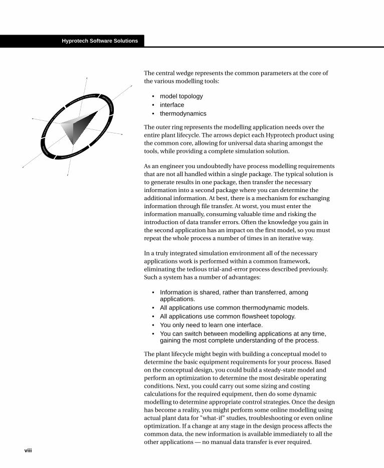
The central wedge represents the common parameters at the core of the various modelling tools:
• model topology• interface• thermodynamics
The outer ring represents the modelling application needs over the entire plant lifecycle. The arrows depict each Hyprotech product using the common core, allowing for universal data sharing amongst the tools, while providing a complete simulation solution.
As an engineer you undoubtedly have process modelling requirements that are not all handled within a single package. The typical solution is to generate results in one package, then transfer the necessary information into a second package where you can determine the additional information. At best, there is a mechanism for exchanging information through file transfer. At worst, you must enter the information manually, consuming valuable time and risking the introduction of data transfer errors. Often the knowledge you gain in the second application has an impact on the first model, so you must repeat the whole process a number of times in an iterative way.
In a truly integrated simulation environment all of the necessary applications work is performed within a common framework, eliminating the tedious trial-and-error process described previously. Such a system has a number of advantages:
• Information is shared, rather than transferred, among applications.
• All applications use common thermodynamic models.• All applications use common flowsheet topology.• You only need to learn one interface.• You can switch between modelling applications at any time,
gaining the most complete understanding of the process.
The plant lifecycle might begin with building a conceptual model to determine the basic equipment requirements for your process. Based on the conceptual design, you could build a steady-state model and perform an optimization to determine the most desirable operating conditions. Next, you could carry out some sizing and costing calculations for the required equipment, then do some dynamic modelling to determine appropriate control strategies. Once the design has become a reality, you might perform some online modelling using actual plant data for "what-if" studies, troubleshooting or even online optimization. If a change at any stage in the design process affects the common data, the new information is available immediately to all the other applications — no manual data transfer is ever required.
Welcome to HYSYS ix
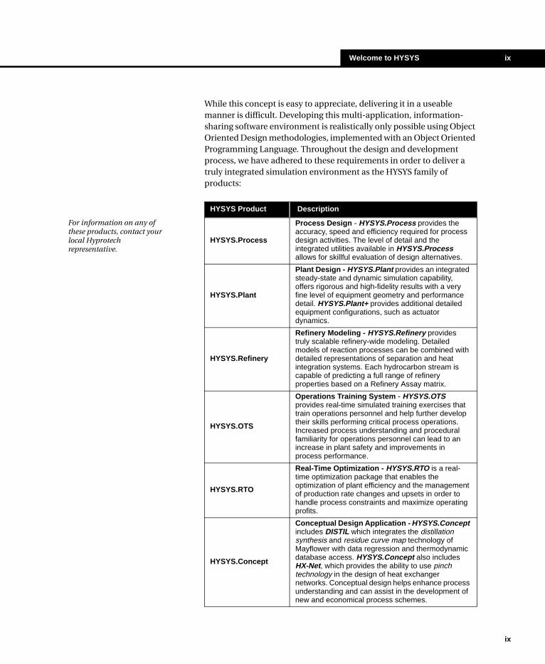
While this concept is easy to appreciate, delivering it in a useable manner is difficult. Developing this multi-application, information-sharing software environment is realistically only possible using Object Oriented Design methodologies, implemented with an Object Oriented Programming Language. Throughout the design and development process, we have adhered to these requirements in order to deliver a truly integrated simulation environment as the HYSYS family of products:
HYSYS Product Description
HYSYS.Process
Process Design - HYSYS.Process provides the accuracy, speed and efficiency required for process design activities. The level of detail and the integrated utilities available in HYSYS.Process allows for skillful evaluation of design alternatives.
HYSYS.Plant
Plant Design - HYSYS.Plant provides an integrated steady-state and dynamic simulation capability, offers rigorous and high-fidelity results with a very fine level of equipment geometry and performance detail. HYSYS.Plant+ provides additional detailed equipment configurations, such as actuator dynamics.
HYSYS.Refinery
Refinery Modeling - HYSYS.Refinery provides truly scalable refinery-wide modeling. Detailed models of reaction processes can be combined with detailed representations of separation and heat integration systems. Each hydrocarbon stream is capable of predicting a full range of refinery properties based on a Refinery Assay matrix.
HYSYS.OTS
Operations Training System - HYSYS.OTS provides real-time simulated training exercises that train operations personnel and help further develop their skills performing critical process operations. Increased process understanding and procedural familiarity for operations personnel can lead to an increase in plant safety and improvements in process performance.
HYSYS.RTO
Real-Time Optimization - HYSYS.RTO is a real-time optimization package that enables the optimization of plant efficiency and the management of production rate changes and upsets in order to handle process constraints and maximize operating profits.
HYSYS.Concept
Conceptual Design Application - HYSYS.Concept includes DISTIL which integrates the distillation synthesis and residue curve map technology of Mayflower with data regression and thermodynamic database access. HYSYS.Concept also includes HX-Net, which provides the ability to use pinch technology in the design of heat exchanger networks. Conceptual design helps enhance process understanding and can assist in the development of new and economical process schemes.
For information on any of these products, contact your local Hyprotech representative.
ix

Hyprotech Software Solutions
x
Intuitive and Interactive Process Modelling
We believe that the role of process simulation is to improve your process understanding so that you can make the best process decisions. Our solution has been, and continues to be, interactive simulation. This solution has not only proven to make the most efficient use of your simulation time, but by building the model interactively – with immediate access to results – you gain the most complete understanding of your simulation.
HYSYS uses the power of Object Oriented Design, together with an Event-Driven Graphical Environment, to deliver a completely interactive simulation environment where:
• calculations begin automatically whenever you supply new information, and
• access to the information you need is in no way restricted.
At any time, even as calculations are proceeding, you can access information from any location in HYSYS. As new information becomes available, each location is always instantly updated with the most current information, whether specified by you or calculated by HYSYS.
Open and Extensible HYSYS Architecture
The Integrated Simulation Environment and our fully Object Oriented software design has paved the way for HYSYS to be fully OLE compliant, allowing for complete user customization. Through a completely transparent interface, OLE Extensibility lets you:
• develop custom steady-state and dynamic unit operations• specify proprietary reaction kinetic expressions• create specialized property packages.
With seamless integration, new modules appear and perform like standard operations, reaction expressions or property packages within HYSYS. The Automation features within HYSYS expose many of the internal Objects to other OLE compliant software like Microsoft Excel, Microsoft Visual Basic and Visio Corporation’s Visio. This functionality enables you to use HYSYS applications as calculation engines for your own custom applications.
By using industry standard OLE Automation and Extension the custom simulation functionality is portable across Hyprotech software updates. The open architecture allows you to extend your simulation functionality in response to your changing needs.
HYSYS is the only commercially available simulation platform designed for complete User Customization.

Welcome to HYSYS xi
Use of the Manuals
HYSYS Electronic Documentation
All HYSYS documentation is available in electronic format as part of the HYSYS Documentation Suite. The HYSYS Documentation CD ROM is included with your package and may be found in the Get Started box. The content of each manual is described in the following table:
The HYSYS Documentation Suite includes all available documentation for the HYSYS family of products.
Manual Description
Get Started
Contains the information needed to install HYSYS, plus a Quick Start example to get you up and running, ensure that HYSYS was installed correctly and is operating properly.
User’s Guide Provides in depth information on the HYSYS interface and architecture. HYSYS Utilities are also covered in this manual.
Simulation Basis
Contains all information relating to the available HYSYS fluid packages and components. This includes information on the Oil Manager, Hypotheticals, Reactions as well as a thermodynamics reference section.
Steady State Modeling
Steady state operation of HYSYS unit operations is covered in depth in this manual.
Dynamic Modeling
This manual contains information on building and running HYSYS simulations in Dynamic mode. Dynamic theory, tools, dynamic functioning of the unit operations as well as controls theory are covered.
This manual is only included with the HYSYS.Plant document set.
Customization Guide
Details the many customization tools available in HYSYS. Information on enhancing the functionality of HYSYS by either using third-party tools to programmatically run HYSYS (Automation), or by the addition of user-defined Extensions is covered. Other topics include the current internally extensible tools available in HYSYS: the User Unit Operation and User Variables as well as comprehensive instruction on using the HYSYS View Editor.
Tutorials Provides step-by-step instructions for building some industry-specific simulation examples.
Applications
Contains a more advanced set of example problems. Note that before you use this manual, you should have a good working knowledge of HYSYS. The Applications examples do not provide many of the basic instructions at the level of detail given in the Tutorials manual.
Quick Reference Provides quick access to basic information regarding all common HYSYS features and commands.
xi

Use of the Manuals
xii
If you are new to HYSYS, you may want to begin by completing one or more of the HYSYS tutorials, which give the step-by-step instructions needed to build a simulation case. If you have some HYSYS experience, but would still like to work through some more advanced sample problems, refer to the HYSYS Applications.
Since HYSYS is totally interactive, it provides virtually unlimited flexibility in solving any simulation problem. Keep in mind that the approach used in solving each example problem presented in the HYSYS documentation may only be one of the many possible methods. You should feel free to explore other alternatives.
Viewing the Online Documentation
HYSYS electronic documentation is viewed using Adobe Acrobat Reader®, which is included on the Documentation CD-ROM. Install Acrobat Reader 4.0 on your computer following the instructions on the CD-ROM insert card. Once installed, you can view the electronic documentation either directly from the CD-ROM, or you can copy the Doc folder (containing all the electronic documentation files) and the file named menu.pdf to your hard drive before viewing the files.
Manoeuvre through the online documentation using the bookmarks on the left of the screen, the navigation buttons in the button bar or using the scroll bars on the side of the view. Blue text indicates an active link to the referenced section or view. Click on that text and Acrobat Reader will jump to that particular section.
Selecting the Search Index
One of the advantages in using the HYSYS Documentation CD is the ability to do power searching using the Acrobat search tools. The Acrobat Search command allows you to perform full text searches of PDF documents that have been indexed using Acrobat Catolog®.
To attach the index file to Acrobat Reader 4.0, use the following procedure:
1. Open the Index Selection view by selecting Edit-Search-Select Indexes from the menu.
2. Click the Add button. This will open the Add Index view.
3. Ensure that the Look in field is currently set to your CD-ROM drive label. There should be two directories visible from the root directory: Acrobat and Doc.
Contact Hyprotech for information on HYSYS training courses.
Ensure that your version of Acrobat Reader has the Search plug-in present. This plug-in allows you to add a search index to the search list.
For more information on the search tools available in Acrobat Reader, consult the help files provided with the program.

Welcome to HYSYS xiii
4. Open the Doc directory. Inside it you should find the Index.pdx file. Select it and click the Open button.
5. The Index Selection view should display the available indexes that can be attached. Select the index name and then click the OK button. You may now begin making use of the Acrobat Search command.
Using the Search Command
The Acrobat Search command allows you to perform a search on PDF documents. You can search for a simple word or phrase, or you can expand your search by using wild-card characters and operators.
To search an index, first select the indexes to search and define a search query. A search query is an expression made up of text and other items to define the information you want to define. Next, select the documents to review from those returned by the search, and then view the occurrences of the search term within the document you selected
Figure 2
Figure 3
xiii

Use of the Manuals
xiv
To perform a full-text search do the following:
1. Choose Edit-Search-Query from the menu.
2. Type the text you want to search for in the Find Results Containing Text box.
3. Click Search. The Search dialog box is hidden, and documents that match your search query are listed in the Search Results window in order of relevancy.
4. Double-click a document that seems likely to contain the relevant information, probably the first document in the list. The document opens on the first match for the text you typed.
5. Click the Search Next button or Search Previous button to go to other matches in the document. Or choose another document to view.
Other Acrobat Reader features include a zoom-in tool in the button bar, which allows you to magnify the text you are reading. If you wish, you may print pages or chapters of the online documentation using the File-Print command under the menu.
Conventions used in the Manuals
The following section lists a number of conventions used throughout the documentation.
Keywords for Mouse Actions
As you work through various procedures in the manuals, you will be given instructions on performing specific functions or commands. Instead of repeating certain phrases for mouse instructions, keywords are used to imply a longer instructional phrase:
Keywords Action
Point Move the mouse pointer to position it over an item. For example, point to an item to see its Tool Tip.
Click
Position the mouse pointer over the item, and rapidly press and release the left mouse button. For example, click Close button to close the current window.
Right-ClickAs for click, but use the right mouse button. For example, right-click an object to display the Object Inspection menu.
These are the normal (default) settings for the mouse, but you can change the positions of the left- and right-buttons.
Welcome to HYSYS xv
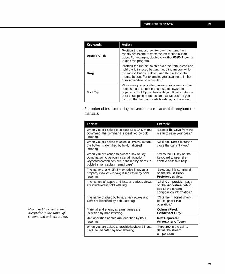
A number of text formatting conventions are also used throughout the manuals:
Double-Click
Position the mouse pointer over the item, then rapidly press and release the left mouse button twice. For example, double-click the HYSYS icon to launch the program.
Drag
Position the mouse pointer over the item, press and hold the left mouse button, move the mouse while the mouse button is down, and then release the mouse button. For example, you drag items in the current window, to move them.
Tool Tip
Whenever you pass the mouse pointer over certain objects, such as tool bar icons and flowsheet objects, a Tool Tip will be displayed. It will contain a brief description of the action that will occur if you click on that button or details relating to the object.
Keywords Action
Format Example
When you are asked to access a HYSYS menu command, the command is identified by bold lettering.
‘Select File-Save from the menu to save your case.’
When you are asked to select a HYSYS button, the button is identified by bold, italicized lettering.
‘Click the Close button to close the current view.’
When you are asked to select a key or key combination to perform a certain function, keyboard commands are identified by words in bolded small capitals (small caps).
‘Press the F1 key on the keyboard to open the context sensitive help.’
The name of a HYSYS view (also know as a property view or window) is indicated by bold lettering.
‘Selecting this command opens the Session Preferences view.’
The names of pages and tabs on various views are identified in bold lettering.
‘Click Composition page on the Worksheet tab to see all the stream composition information.’
The name of radio buttons, check boxes and cells are identified by bold lettering.
‘Click the Ignored check box to ignore this operation.’
Material and energy stream names are identified by bold lettering.
Column Feed, Condenser Duty
Unit operation names are identified by bold lettering.
Inlet Separator, Atmospheric Tower
When you are asked to provide keyboard input, it will be indicated by bold lettering.
‘Type 100 in the cell to define the stream temperature.’
Note that blank spaces are acceptable in the names of streams and unit operations.
xv
Use of the Manuals
xvi
Bullets and Numbering
Bulleted and numbered lists will be used extensively throughout the manuals. Numbered lists are used to break down a procedure into steps, for example:
1. Select the Name cell.
2. Type a name for the operation.
3. Press ENTER to accept the name.
Bulleted lists are used to identify alternative steps within a procedure, or for simply listing like objects. A sample procedure that utilizes bullets is:
1. Move to the Name cell by doing one of the following:
• Select the Name cell• Press ALT N
2. Type a name for the operation.
• Press ENTER to accept the name.
Notice the two alternatives for completing Step 1 are indented to indicate their sequence in the overall procedure.
A bulleted list of like objects might describe the various groups on a particular view. For example, the Options page of the Simulation tab on the Session Preferences view has three groups, namely:
• General Options• Errors• Column Options
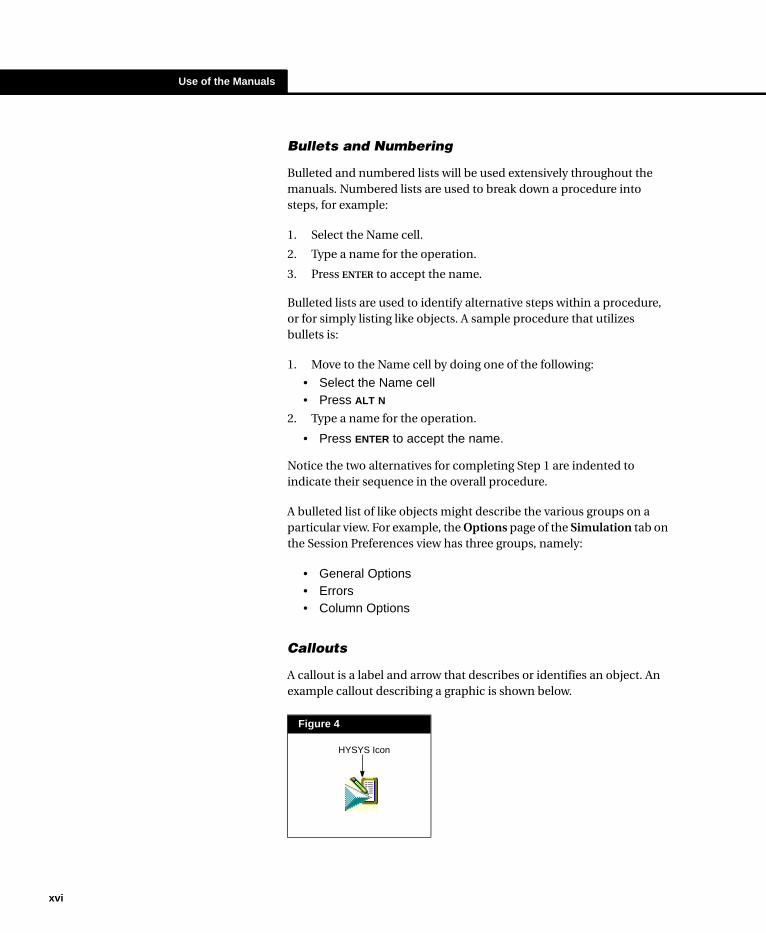
Callouts
A callout is a label and arrow that describes or identifies an object. An example callout describing a graphic is shown below.
Figure 4
HYSYS Icon

Welcome to HYSYS xvii
Annotations
Text appearing in the outside margin of the page supplies you with additional or summary information about the adjacent graphic or paragraph. An example is shown to the left.
Shaded Text Boxes
A shaded text box provides you with important information regarding HYSYS’ behaviour, or general messages applying to the manual. Examples include:
The use of many of these conventions will become more apparent as you progress through the manuals.
Annotation text appears in the outside page margin.
The resultant temperature of the mixed streams may be quite different than those of the feed streams, due to mixing effects.
Before proceeding, you should have read the introductory section which precedes the example problems in this manual.
xvii

Use of the Manuals
xviii

xix
Technical SupportThere are several ways in which you can contact Technical Support. If you cannot find the answer to your question in the manuals, we encourage you to visit our Website at www.hyprotech.com, where a variety of information is available to you, including:
• answers to frequently asked questions• example cases and product information• technical papers• news bulletins• hyperlink to support email
You can also access Support directly via email. A listing of Technical Support Centres including the Support email address is at the end of this chapter. When contacting us via email, please include in your message:
• Your full name, company, phone and fax numbers.• The version of HYSYS you are using (shown in the Help, About
HYSYS view).• The serial number of your HYSYS security key.• A detailed description of the problem (attach a simulation case
if possible).
We also have toll free lines that you may use. When you call, please have the same information available.
xix

xx
Technical Support CentresCalgary, Canada
AEA Technology - Hyprotech Ltd.
Suite 800, 707 - 8th Avenue SW
Calgary, Alberta
T2P 1H5
[email protected] (email)
(403) 520-6181 (local - technical support)
1-888-757-7836 (toll free - technical support)
(403) 520-6601 (fax - technical support)
1-800-661-8696 (information & sales)
Barcelona, Spain (Rest of Europe)
AEA Technology - Hyprotech Ltd.
Hyprotech Europe S.L.
Pg. de Gràcia 56, 4th floor
E-08007 Barcelona, Spain
[email protected] (email)
+34 93 215 68 84 (technical support)
900 161 900 (toll free - technical support - Spain only)
+34 93 215 42 56 (fax - technical support)
+34 93 215 68 84 (information & sales)
Oxford, UK (UK clients only)
AEA Technology Engineering Software
Hyprotech Ltd.
404 Harwell, Didcot
Oxfordshire, OX11 0QJ
United Kingdom
[email protected] (email)
0800 7317643 (freephone technical support)
+44 1235 434351 (fax - technical support)
+44 1235 435555 (information &
sales)
Kuala Lumpur, Malaysia
AEA Technology - Hyprotech Ltd.
Hyprotech Ltd., Malaysia
Lot E-3-3a, Dataran Palma
Jalan Selaman ½, Jalan Ampang
68000 Ampang, Selangor
Malaysia
[email protected] (email)
+60 3 4270 3880 (technical support)
+60 3 4271 3811 (fax - technical support)
+60 3 4270 3880 (information & sales)
Yokohama, Japan
AEA Technology - Hyprotech Ltd.
AEA Hyprotech KK
Plus Taria Bldg. 6F.
3-1-4, Shin-Yokohama
Kohoku-ku
Yokohama, Japan
222-0033
[email protected] (email)
81 45 476 5051 (technical support)
81 45 476 5051 (information & sales)
xx
xxi
OfficesCalgary, Canada
Tel: (403) 520-6000
Fax: (403) 520-6040/60
Toll Free: 1-800-661-8696
Yokohama, Japan
Tel: 81 45 476 5051
Fax: 81 45 476 3055
Newark, DE, USA
Tel: (302) 369-0773
Fax: (302) 369-0877
Toll Free: 1-800-688-3430
Houston, TX, USA
Tel: (713) 339-9600
Fax: (713) 339-9601
Toll Free: 1-800-475-0011
Oxford, UK
Tel: +44 1235 435555
Fax: +44 1235 434294
Barcelona, Spain
Tel: +34 93 215 68 84
Fax: +34 93 215 42 56
Oudenaarde, Belgium
Tel: +32 55 310 299
Fax: +32 55 302 030
Düsseldorf, Germany
Tel: +49 211 577933 0
Fax: +49 211 577933 11
Hovik, Norway
Tel: +47 67 10 6464
Fax: +47 67 10 6465
Cairo, Egypt
Tel: +20 2 7020824
Fax: +20 2 7020289
Kuala Lumpur, Malaysia
Tel: +60 3 4270 3880
Fax: +60 3 4270 3811
Seoul, Korea
Tel: 82 2 3453 3144 5
Fax: 82 2 3453 9772
xxi
xxii
Agents
InternetWebsite: www.hyprotech.com
Email: [email protected]
International Innotech, Inc.Katy, USA
Tel: (281) 492-2774Fax: (281) 492-8144
International Innotech, Inc. Beijing, China
Tel: 86 10 6499 3956 Fax: 86 10 6499 3957
International InnotechTaipei, Taiwan
Tel: 886 2 809 6704Fax: 886 2 809 3095
KBTECH Ltda. Bogota, Colombia
Tel: 57 1 258 44 50 Fax: 57 1 258 44 50
India PVT Ltd.Pune, India
Tel: 91 020 5510141 Fax: 91 020 5510069
Logichem Process Johannesburg, South Africa
Tel: 27 11 465 3800 Fax: 27 11 465 4548
Plant Solutions Pty. Ltd. Peregian, Australia
Tel: 61 7 544 81 355Fax: 61 7 544 81 644
Protech Engineering Bratislava, Slovak Republic
Tel: +421 7 4488 8286 Fax: +421 7 4488 8286
PT. Danan Wingus SaktiJakarta, Indonesia
Tel: 62 21 567 4573 75/62 21 567 4508 10Fax: 62 21 567 4507/62 21 568 3081
Ranchero Services (Thailand) Co. Ltd.Bangkok, Thailand
Tel: 66 2 381 1020Fax: 66 2 381 1209
S.C. Chempetrol Service srl Bucharest, Romania
Tel: +401 330 0125Fax: +401 311 3463
Soteica De Mexico Mexico D.F., Mexico
Tel: 52 5 546 5440Fax: 52 5 535 6610
Soteica Do Brasil Sao Paulo, Brazil
Tel: 55 11 533 2381 Fax: 55 11 556 10746
Soteica S.R.L. Buenos Aires, Argentina
Tel: 54 11 4555 5703 Fax: 54 11 4551 0751
Soteiven C.A. Caracas, Venezuela
Tel: 58 2 264 1873Fax: 58 2 265 9509
ZAO Techneftechim Moscow, Russia
Tel: +7 095 202 4370Fax: +7 095 202 4370
xxii

xxiii
HYSYS Hot Keys
FileCreate New Case CTRL+NOpen Case CTRL+OSave Current Case CTRL+SSave As... CTRL+SHIFT+SClose Current Case CTRL+ZExit HYSYS ALT+F4 SimulationGo to Basis Manager CTRL+B Leave Current Environment (Return to Previous)
CTRL+L
Main Properties CTRL+MAccess Optimizer F5Toggle Steady-State/Dynamic Modes
F7
Toggle Hold/Go Calculations F8Access Integrator CTRL+IStart/Stop Integrator F9Stop Calculations CTRL+BREAKFlowsheetAdd Material Stream F11Add Operation F12Access Object Navigator F3 Show/Hide Object Palette F4Composition View (from Workbook)
CTRL+K
ToolsAccess Workbooks CTRL+WAccess PFDs CTRL+PToggle Move/Attach (PFD) CTRLAccess Utilities CTRL+UAccess Reports CTRL+RAccess DataBook CTRL+DAccess Controller FacePlates CTRL+FAccess Help F1ColumnGo to Column Runner (SubFlowsheet)
CTRL+T
Stop Column Solver CTRL+BREAKWindowClose Active Window CTRL+F4Tile Windows SHIFT+F4Go to Next Window CTRL+F6 or CTRL+TABGo to Previous Window CTRL+SHIFT+F6 orEditing/General CTRL+SHIFT+TABAccess Edit Bar F2Access Pull-Down Menus F10 or ALTGo to Next Page Tab CTRL+SHIFT+NGo to Previous Page Tab CTRL+SHIFT+PCut CTRL+XCopy CTRL+CPaste CTRL+V
xxiii

xxiv
xxiv

Steady State Modeling 1-1
1 Steady State Modeling
1-1
1.1 Engineering................................................................................................... 3
1.2 Operations .................................................................................................... 6
1.2.1 Installing Operations ................................................................................ 61.2.2 The Unit Operation Property View ........................................................... 7

1-2
1-2
Steady State Modeling 1-3
1.1 EngineeringAs you have seen in the User’s Guide and Simulation Basis manual, HYSYS has been uniquely created with respect to the program architecture, interface design, engineering capabilities and interactive operation. The integrated steady state and dynamic modeling capabilities, where the same model can be evaluated from either perspective with full sharing of process information, represents a significant advancement in the industry.
The various components that make up HYSYS have produced an extremely powerful approach to steady-state process modeling. At a fundamental level, the comprehensive selection of operations and property methods allows you to model a wide range of processes with confidence. Perhaps even more important is how the HYSYS approach to modeling maximizes your return on simulation time through increased process understanding.
The key to this last fact is the Event Driven operation. By using a degrees of freedom approach, calculations in HYSYS are performed automatically. HYSYS performs calculations as soon as unit operations and property packages have enough required information. Any results, including passing partial information when a complete calculation cannot be performed, is propagated bi-directionally throughout the Flowsheet. What this means is that you can start your simulation in any location, using the available information to its greatest advantage. Since results are available immediately - including as calculations are being performed - you gain the greatest understanding of each individual aspect of your process.
The multi-flowsheet architecture of HYSYS is vitally important to this overall approach to modeling. Although HYSYS has been designed to allow the use of multiple property packages and the creation of pre-built templates, the greatest advantage of multi-flowsheeting is that it provides an extremely effective way to organize large processes. By breaking Flowsheets into smaller components, you can easily isolate any aspect for detailed analysis. Each of these sub-processes is part of the overall simulation, automatically calculating like any other operation.
The design of the HYSYS interface is consistent, if not integral, with this approach to modeling. Access to information is the most important aspect of successful modeling, with accuracy and capabilities accepted as fundamental requirements. Not only can you access whatever information you need when you need it, but the same information can
1-3
1-4 Engineering
1-4
be displayed simultaneously in a variety of locations. Just as there is no standardized way to build a model, there is no unique way to look at results. HYSYS uses a variety of methods to display process information - individual property views, the PFD, Workbook, DataBook, graphical Performance Profiles and Tabular Summaries. Not only are all of these display types simultaneously available, but through the object-oriented design, every piece of displayed information is automatically updated whenever conditions change.
The inherent flexibility of HYSYS allows for the use of third party design options and custom-built unit operations. These can be linked to HYSYS through OLE Extensibility.
This Engineering section covers the various unit operations, Template and Column Sub-Flowsheet models, Optimization, Utilities, and Dynamics. Since HYSYS is an integrated steady state and dynamic modeling package, the steady state and dynamic modeling capabilities of each unit operation will be described successively, thus illustrating how the information is shared between the two approaches. In addition to the Physical operations, there is a chapter for Logical operations, which are the operations that do not physically perform heat and material balance calculations, but rather, impart logical relationships between the elements that make up your process.
The following is a brief definition of categories used in this volume:
Integrated into the steady state modeling is multi-variable optimization. Once you have reached a converged solution, you can construct virtually any objective function with the Optimizer. There are
Term Definition
Physical Operations Governed by thermodynamics and mass/energy balances, as well as operation-specific relations.
Logical Operations
The Logical Operations presented in this volume are primarily used in Steady State mode to establish numerical relationships between variables. Examples include the ADJUST and RECYCLE. There are, however, several operations such as the SPREADSHEET and SET operation which can be used in Steady State and Dynamics mode.
Sub-Flowsheets
You can define processes in a Sub-Flowsheet, which can then be inserted as a "unit operation" into any other Flowsheet. You have full access to the operations normally available in the Main Flowsheet.
Columns
Unlike the other unit operations, the HYSYS COLUMN is contained within a separate Sub-Flowsheet, which appears as a single operation in the Main Flowsheet.
Steady State Modeling 1-5
five available solution algorithms for both unconstrained and constrained optimization problems, with an automatic backup mechanism when the Flowsheet moves into a region of non-convergence.
HYSYS offers an assortment of utilities which can be attached to process streams and unit operations. These tools interact with the process and provide additional information.
In this manual, each operation is explained in its respective chapters for steady state modeling. A separate manual has been devoted to the principles behind dynamic modeling. HYSYS is the first simulation package to offer dynamic Flowsheet modeling backed up by rigorous property package calculations. As there is not the same wealth of process modeling experience in this area as there is for steady state modeling, information regarding the dynamic response of a model has been included in the Dynamic Modelling guide to ensure that you will realize the greatest benefit of this revolutionary product
HYSYS has a number of unit operations which can be used to assemble Flowsheets. By connecting the proper unit operations and streams, you can model a wide variety of oil, gas, petrochemical and chemical processes.
Included in the available operations are those which are governed by thermodynamics and mass/energy balances, such as HEAT EXCHANGERS, SEPARATORS and COMPRESSORS, and the logical operations like the ADJUST, SET and RECYCLE. A number of operations are also included specifically for dynamic modeling, such as the CONTROLLER, TRANSFER FUNCTION BLOCK and SELECTOR. The SPREADSHEET is a powerful tool which provides a link to nearly any Flowsheet variable, allowing you to model "special" effects not otherwise available in HYSYS.
In modeling operations, HYSYS uses a Degrees of Freedom approach, which increases the flexibility with which solutions are obtained. For most operations, you are not constrained to provide information in a specific order, or even to provide a specific set of information. As you provide information to the operation, HYSYS will calculate any unknowns that can be determined based on what you have entered.
For instance, consider the PUMP operation. If you provide a fully-defined inlet stream to the pump, HYSYS will immediately pass the composition and flow to the outlet. If you then provide a percent efficiency and pressure rise, the outlet and energy streams will be fully defined. If, on the other hand, the flowrate of the inlet stream is
For more information on Dynamic Modelling unit operations, consult the Dynamic Modelling guide.
1-5
1-6 Operations
1-6
undefined, HYSYS will not be able to calculate any outlet conditions until you provide three parameters, such as the efficiency, pressure rise, and work. In the case of the PUMP operation, there are three degrees of freedom, thus, three parameters are required to fully define the outlet stream.
All information concerning a unit operation can be found on the tabs and pages of its property view. Each tab in the property view contains pages which pertain to a certain aspect of the operation, such as its stream connections, physical parameters (for example: pressure drop and energy input), or dynamic parameters such as vessel rating and valve information.
1.2 Operations
1.2.1 Installing OperationsThere are a number of ways to install unit operations into your Flowsheet. The operations which are available will depend on where you are currently working (Main Flowsheet, Template Sub-Flowsheet or Column Sub-Flowsheet). If you are in the Main or Template environments, all operations will be available, except those associated specifically with the column, such as reboilers and condensers. A smaller set of operations is available within the Column Sub-Flowsheet.
For detailed information on installing unit operations, refer to Section 1.3.3 - Object Palette or Section 1.3.5 - Installing Operations in the User’s Guide.
The two primary areas from which you can install operations are the UnitOps view and the Object Palette.
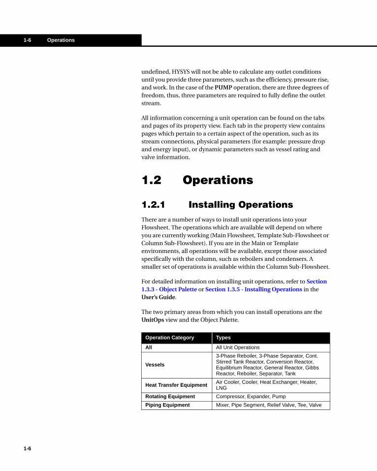
Operation Category Types
All All Unit Operations
Vessels
3-Phase Reboiler, 3-Phase Separator, Cont. Stirred Tank Reactor, Conversion Reactor, Equilibrium Reactor, General Reactor, Gibbs Reactor, Reboiler, Separator, Tank
Heat Transfer Equipment Air Cooler, Cooler, Heat Exchanger, Heater, LNG
Rotating Equipment Compressor, Expander, Pump
Piping Equipment Mixer, Pipe Segment, Relief Valve, Tee, Valve
Steady State Modeling 1-7
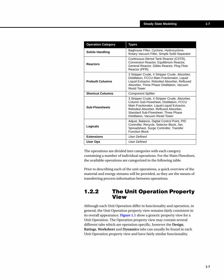
The operations are divided into categories with each category containing a number of individual operations. For the Main Flowsheet, the available operations are categorized in the following table.
Prior to describing each of the unit operations, a quick overview of the material and energy streams will be provided, as they are the means of transferring process information between operations.
1.2.2 The Unit Operation Property View
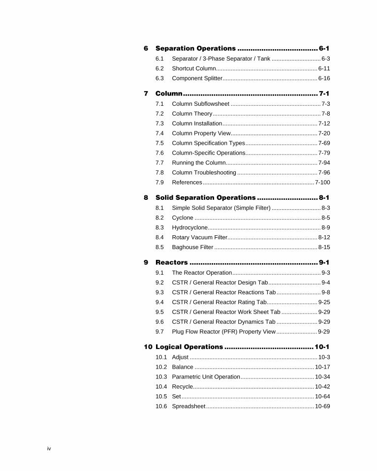
Although each Unit Operation differ in functionality and operation, in general, the Unit Operation property view remains fairly consistent in its overall appearance. Figure 1.1 show a generic property view for a Unit Operation. The Operation property view may contain several different tabs which are operation specific, however the Design, Ratings, Worksheet and Dynamics tabs can usually be found in each Unit Operation property view and have fairly similar functionality.
Solids Handling Baghouse Filter, Cyclone, Hydrocyclone, Rotary Vacuum Filter, Simple Solid Separator
Reactors
Continuous-Stirred Tank Reactor (CSTR), Conversion Reactor, Equilibrium Reactor, General Reactor, Gibbs Reactor, Plug Flow Reactor (PFR)
Prebuilt Columns
3 Stripper Crude, 4 Stripper Crude, Absorber, Distillation, FCCU Main Fractionator, Liquid-Liquid Extractor, Reboiled Absorber, Refluxed Absorber, Three Phase Distillation, Vacuum Resid Tower
Shortcut Columns Component Splitter
Sub-Flowsheets
3 Stripper Crude, 4 Stripper Crude, Absorber, Column Sub-Flowsheet, Distillation, FCCU Main Fractionator, Liquid-Liquid Extractor, Reboiled Absorber, Refluxed Absorber, Standard Sub-Flowsheet, Three Phase Distillation, Vacuum Resid Tower
Logicals
Adjust, Balance, Digital Control Point, PID Controller, Recycle, Selector Block, Set, Spreadsheet, Surge Controller, Transfer Function Block
Extensions User Defined
User Ops User Defined
Operation Category Types
1-7

1-8 Operations
1-8
Figure 1.1
The Name of the Unit Operation
The various pages of the active tab.
The active tab of the property view.
Deletes this Unit Operation from the Flowsheet.
Displays the calculation status of this Unit Operation. It may also display what specifications are required.
Ignores this Unit Operation.
Tab Description
Design
Connects the feed and product streams to the Unit Operation. Other parameters such as pressure drop, heat flow and solving method are also specified on the various pages of this tab.
RatingsRates and Sizes the Unit Operation vessel. Specification of the tab is not always necessary in Steady State mode, however it can be used to calculate vessel hold up.
WorksheetDisplays the Conditions, Properties, Composition and Pressure Flow values of the streams entering and exiting the Unit Operation.
Dynamics
Sets the dynamic parameters associated with this Unit Operation such valve sizing and pressure flow relations. Not relevant to Steady State modeling. For information on Dynamic Modelling implications of this tab, consult the Dynamic Modelling guide.
Streams 2-1
2 Streams
2-1
2.1 Material Stream Property View.................................................................... 3
2.1.1 Worksheet Tab ......................................................................................... 42.1.2 Attachments Tab .....................................................................................112.1.3 Dynamics Tab .........................................................................................112.1.4 User Variables Tab ..................................................................................11
2.2 Energy Stream Property View ................................................................... 12
2.2.1 Stream Tab............................................................................................. 122.2.2 Unit Ops Tab .......................................................................................... 132.2.3 Dynamics Tab ........................................................................................ 132.2.4 User Variables Tab ................................................................................. 13

2-2
2-2

Streams 2-3
2.1 Material Stream Property View
Material Streams are added to a simulation in the Main Simulation Environment, where you can define their properties and composition. There are several ways to add a Material Stream, represented on the Object Palette by a blue arrow, to your simulation. One of the simplest ways to install a Material Stream is by pressing the F11 key. For information on other available methods, refer to Section 3.3 - Installing Streams and Operations in the User’s Guide.
The Material Stream property view contains several tabs and associated pages that allow you to define parameters, view properties, add utilities and specify dynamic information. Figure 2.1 shows the initial view of a new Material Stream after it has been added to a simulation.
The buttons and Status Bar at the bottom of the view are always visible when the Material Stream view is open. If you want to copy properties or compositions from existing streams from your flowsheet, you can do so by pressing the Define from Other Stream button. This button opens a window from which you can choose the stream properties and/or compositions you want to copy to your stream.
The buttons with the green arrows to the left of the Status Bar are the View Upstream Operation and View Downstream Operation buttons.
Figure 2.1
Material Stream Button
(Blue Arrow)
View Upstream Operation Button
View Downstream Operation Button
2-3
2-4 Material Stream Property View
2-4
The left-pointing arrow indicates the downstream position and the right-pointing arrow the upstream position. If the stream you are looking at is attached to an operation, selecting these buttons will open the property view of the nearest upstream or downstream operation. If the stream is not connected to an operation at the upstream or downstream end, then these buttons will open a Feeder Block or a Product Block.
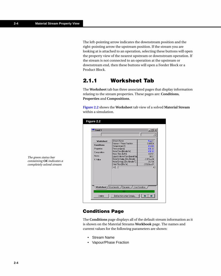
2.1.1 Worksheet TabThe Worksheet tab has three associated pages that display information relating to the stream properties. These pages are: Conditions, Properties and Compositions.
Figure 2.2 shows the Worksheet tab view of a solved Material Stream within a simulation.
Conditions Page
The Conditions page displays all of the default stream information as it is shown on the Material Streams Workbook page. The names and current values for the following parameters are shown:
• Stream Name• Vapour/Phase Fraction
Figure 2.2
The green status bar containing OK indicates a completely solved stream

Streams 2-5
• Temperature• Pressure• Molar Flow• Mass Flow• LiqVol Flow• Molar Enthalpy• Molar Entropy• Heat Flow
HYSYS uses degrees of freedom in combination with built-in intelligence, to automatically perform flash calculations. In order for a stream to "flash", the following information must be specified (either from your specifications or as a result of other Flowsheet calculations):
• Stream Composition
Two of the following properties must also be specified; at least one of the specifications must be temperature or pressure:
• Temperature• Pressure• Vapour Fraction• Entropy• Enthalpy
Depending on which of the state variables are known, HYSYS will automatically perform the correct flash calculation.
Once a stream has flashed, all other properties about the stream are calculated as well. You can examine these properties through the additional pages of the property view. Note that a flowrate is required to calculate the Heat Flow.
The Stream parameters may be specified on the Conditions page or in the Workbook. Changes in one area will be reflected throughout the Flowsheet.
Note that while the Workbook displays the bulk conditions of the stream, the Conditions, Properties and Compositions pages will also show the values for the individual phase conditions. HYSYS can display up to five different phases.
At least one of the temperature or pressure properties must be specified for the material stream to solve.
Note that if you specify a vapour fraction of 0 or 1, the stream is assumed to be at the bubble point or dew point, respectively. You can also specify vapour fractions between 0 and 1.
2-5
2-6 Material Stream Property View
2-6
• Overall• Vapour• Liquid• Aqueous• Second Liquid• Mixed Liquid
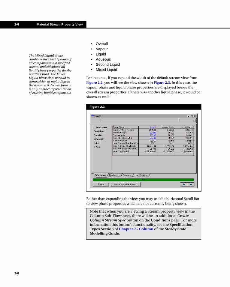
For instance, if you expand the width of the default stream view from Figure 2.2, you will see the view shown in Figure 2.3. In this case, the vapour phase and liquid phase properties are displayed beside the overall stream properties. If there was another liquid phase, it would be shown as well.
Rather than expanding the view, you may use the horizontal Scroll Bar to view phase properties which are not currently being shown.
Figure 2.3
The Mixed Liquid phase combines the Liquid phases of all components in a specified stream, and calculates all liquid phase properties for the resulting fluid. The Mixed Liquid phase does not add its composition or molar flow to the stream it is derived from, it is only another representation of existing liquid components
Note that when you are viewing a Stream property view in the Column Sub-Flowsheet, there will be an additional Create Column Stream Spec button on the Conditions page. For more information this button’s functionality, see the Specification Types Section of Chapter 7 - Column of the Steady State Modelling Guide.

Streams 2-7
Properties Page
The Properties page shows all the Transport Properties for each stream phase. These properties include:
Expand the view or use the scroll bar to view the individual phase parameters, as shown in Figure 2.4. None of the parameters shown on this page (i.e., the parameters shown in black) can be edited, since they are dependent on the basic stream conditions (pressure, temperature, compositions, etc.)
• Vapour / Phase Fraction • Vap. Frac. (mass basis)
• Temperature • Vap. Frac. (volume basis)
• Pressure • Molar Volume
• Actual Vol. Flow • Act. Gas Flow
• Mass Enthalpy • Act. Liq. Flow
• Mass Entropy • Std. Liq. Flow
• Molecular Weight • Std. Gas Flow
• Molar Density • Watson K
• Mass Density • Kinematic Viscosity
• Std. Liquid Mass Density • Cp/Cv
• Molar Heat Capacity • Lower Heating Value
• Mass Heat Capacity • Mass Lower Heating Value
• Thermal Conductivity • Liquid Fraction
• Viscosity • Partial Pressure of CO2
• Surface Tension • Avg. Liq. Density
• Specific Heat • Heat of Vap.
• Z Factor • Mass Heat of Vap.
• Vap. Frac. (molar basis) •
The Heat of Vapourisation for a stream in HYSYS, is defined as the heat required to go from saturated liquid to saturated vapour.
2-7

2-8 Material Stream Property View
2-8
Composition Page
Select Composition on the Worksheet tab to view the Composition page for the Material Stream. You can specify or change the stream composition by either pressing the Edit button or by entering a value in a worksheet cell and pressing ENTER. Either action will access the Input Composition view.
For the example shown in Figure 2.5, the mole fractions for each component in the overall phase, the vapour phase and the aqueous phase are displayed. You may view the composition in a different basis by selecting the Basis button.
Figure 2.4
You are unable to change the composition of streams calculated by HYSYS. The default colour for specified stream values is blue and black for those calculated by HYSYS.

Streams 2-9
After pressing the Basis button, you can select one of the radio buttons on the Stream dialog to choose a new compositional basis. After pressing the Close button, the stream compositions will be shown using the new basis.
Pressing the Edit button in the Material Stream property view opens the Input Composition dialog. When working in the Input Composition dialog you can edit the compositions by selecting a radio button in the Composition Basis group and entering the compositions into the appropriate cells.
The Composition Controls group has two buttons that can be used to manipulate the compositions.
Figure 2.5
Close Button
For fractional bases, selecting the OK button automatically normalizes the composition if all compositions contain a value. The Cancel button closes the dialog without accepting any changes.
You will not be able to edit the compositions for a stream that is calculated by HYSYS. When you move to the Comp page for such a stream, the Edit button will be inaccessible.
2-9

2-10 Material Stream Property View
2-10
K Value Page
The K Value page displays the K values or distribution coefficients for each component in the stream. A distribution coefficient is a ratio between the mole fraction of component i in the vapour phase and the mole fraction of component i in the liquid phase:
where: Ki = Distribution Coefficient
yi = mole fraction of component i in the vapour phase
xi = mole fraction of component i in the liquid phase
Composition Control Button
Action
Erase Clears all compositions.
Normalize
Allows you to enter any value for fractional compositions and has HYSYS normalize the values such that the total equals 1. This button is useful when many components are available, but you wish to supply compositions for only a few. When you enter the compositions, press the Normalize button and HYSYS will ensure the Total is 1.0, while also specifying any <empty> compositions as zero. If compositions are left as <empty>, HYSYS will not perform the flash calculation on the stream. Note that the Normalize button does not apply to flow compositional bases, since there is no restriction on the total flowrate.
Figure 2.6
Ki
yi
xi----=
Streams 2-11
Notes Page
You can use this page to add any notes pertinent to the unit operation or the simulation case in general.
2.1.2 Attachments Tab
Unit Ops Page
On the Unit Ops page, you can view the names and types of unit operations and logicals to which the stream is attached. The view shows three groups:
• The units from which the stream is a product.• The units to which the stream is a feed.• The logicals to which the stream is connected.
You can access the property view for the specific unit operation or logical by double clicking on a Name or Type cell.
Utilities Page
The options on the Utilities page allow you to:
• Attach Utilities to the current Stream. • View existing Utilities that are attached to the Stream.• Delete existing Utilities that are attached to the Stream.
2.1.3 Dynamics TabThe options on the Dynamics tab allow you to set the dynamic specifications for a simulation. Unless you plan to run the case in Dynamics mode, you are not required to change any of the information available on the Specs page of this tab.
2.1.4 User Variables TabOn this tab you can create and implement your own User Variables for use in a HYSYS simulation. For more information on User Variables see the User Variables chapter in the Customization Guide.
2-11
2-12 Energy Stream Property View
2-12
2.2 Energy Stream Property View
Energy Streams are represented by the red arrow button on the Tool Palette. One method of adding an Energy Stream is by pressing this button and then clicking on the PFD. This method will immediately access the Energy Stream property view. You can also open the Energy Stream view from the Energy Streams page of the Workbook by double clicking in a cell associated with the stream.
The Energy Stream view contains four tabs which allow you to define stream parameters, view objects to which the stream is attached and specify dynamic information. These tabs are: Streams, Unit Ops, Dynamics and User Variables.
As with the Material streams, the Energy Stream view has View Upstream Operation and View Downstream Operation buttons that allow you to view the unit operation to which the stream is connected. However, Energy streams differ from Material streams in that if there is no upstream or downstream connection on the stream (which is often the case for Energy stream) the associated button will not be active.
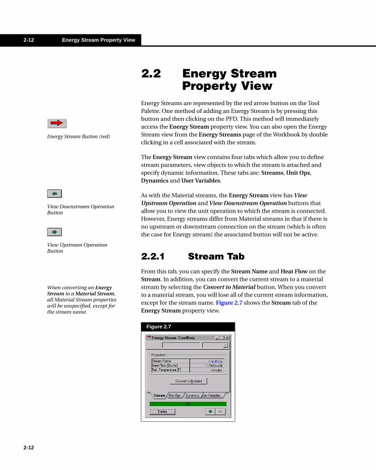
2.2.1 Stream TabFrom this tab, you can specify the Stream Name and Heat Flow on the Stream. In addition, you can convert the current stream to a material stream by selecting the Convert to Material button. When you convert to a material stream, you will lose all of the current stream information, except for the stream name. Figure 2.7 shows the Stream tab of the Energy Stream property view.
Figure 2.7
Energy Stream Button (red)
View Downstream Operation Button
View Upstream Operation Button
When converting an Energy Stream to a Material Stream, all Material Stream properties will be unspecified, except for the stream name.

Streams 2-13
2.2.2 Unit Ops TabThe Unit Ops tab displays the Names and Types of all objects to which the Energy stream is attached. Both unit operations and logicals are listed. The Unit Ops tab will either show a unit operation in the Product From cell or in the Feed To cell, depending on whether the Energy stream receives or provides energy respectively.
You can double click on either the Product From or Feed To cell to access the property view of the operation attached to the stream.
2.2.3 Dynamics TabThe options on the Dynamics tab allow you to set the dynamic specifications for a simulation. Unless you plan to run the case in dynamic mode, you are not required to change any of the information available on the Specs page of this tab.
2.2.4 User Variables TabOn this tab you can create and implement User Variables for use in your HYSYS simulation. For more information on working with User Variables, see the User Variable chapter in the Customization Guide.
Figure 2.8
2-13

2-14 Energy Stream Property View
2-14

Heat Transfer Equipment 3-1
3 Heat Transfer Equipment
3.1 Air Cooler ...................................................................................................... 3
3.1.1 Theory...................................................................................................... 33.1.2 Design Tab ............................................................................................... 43.1.3 Rating Tab................................................................................................ 63.1.4 Worksheet Tab ......................................................................................... 73.1.5 Performance Tab...................................................................................... 73.1.6 Dynamics Tab .......................................................................................... 83.1.7 Air Cooler Example .................................................................................. 9
3.2 Cooler/Heater.............................................................................................. 11
3.2.1 Theory.....................................................................................................113.2.2 Design Tab ..............................................................................................113.2.3 Rating Tab.............................................................................................. 133.2.4 Worksheet Tab ....................................................................................... 143.2.5 Performance Tab.................................................................................... 143.2.6 Dynamics Tab ........................................................................................ 163.2.7 Example - Gas Cooler............................................................................ 16
3.3 Heat Exchanger .......................................................................................... 18
3.3.1 Theory.................................................................................................... 193.3.2 Design Tab ............................................................................................. 203.3.3 Rating Tab.............................................................................................. 303.3.4 Worksheet Tab ....................................................................................... 433.3.5 Performance Tab.................................................................................... 443.3.6 Dynamics Tab ........................................................................................ 463.3.7 Heat Exchanger Examples..................................................................... 46
3.4 Fired Heater (Furnace) ............................................................................... 49
3-1

3-2
3-2
3.5 LNG.............................................................................................................. 49
3.5.1 Design Tab ............................................................................................. 503.5.2 Rating Tab.............................................................................................. 573.5.3 Worksheet Tab ....................................................................................... 573.5.4 Performance Tab.................................................................................... 583.5.5 Dynamics Tab ........................................................................................ 613.5.6 HTFS-MUSE Tab ................................................................................... 613.5.7 LNG Example......................................................................................... 78

Heat Transfer Equipment 3-3
3.1 Air CoolerThe AIR COOLER unit operation uses an ideal air mixture as a heat transfer medium to cool (or heat) an inlet process stream to a required exit stream condition. One or more fans circulate the air through bundles of tubes to cool process fluids. The air flow can be specified or calculated from the fan rating information. The AIR COOLER can solve for many different sets of specifications including:
• The overall heat transfer coefficient, UA• The total air flow• The exit stream temperature
To install the AIR COOLER operation, press F12 and choose Air Cooler from the UnitOps view or select the Air Cooler button in the Object Palette.
To ignore the AIR COOLER, select the Ignore check box. HYSYS will completely disregard the operation (and will not calculate the outlet stream) until you restore it to an active state by clearing the check box.
3.1.1 TheoryThe AIR COOLER uses the same basic equation as the HEAT EXCHANGER unit operation. However, the air cooler operation can calculate the flow of air based on the fan rating information.
The AIR COOLER calculations are based on an energy balance between the air and process streams. For a cross-current air cooler, the energy balance is shown as follows:
where: Mair = Air stream mass flow rate
Mprocess = Process stream mass flow rate
H = Enthalpy
Air Cooler Button
Mair(Hout - Hin)air = Mprocess(Hin - Hout)process (3.1)
3-3

3-4 Air Cooler
3-4
The AIR COOLER duty, Q, is defined in terms of the overall heat transfer coefficient, the area available for heat exchange and the log mean temperature difference:
where: U = Overall heat transfer coefficient
A = Surface area available for heat transfer
DTLM = Log mean temperature difference (LMTD)
Ft = correction factor
The LMTD correction factor, Ft, is calculated from the geometry and configuration of the air cooler.
3.1.2 Design TabThe Design tab provides access to four pages: the Connections, Parameters, User Variables and Notes page.
Connections Page
On the Connections page, provide the names of the Feed and Product streams attached to the AIR COOLER. You can change the name of the operation in the Name cell. Figure 3.1 shows the Connections page for the Air Cooler.
Q = -UADTLMFt (3.2)
Figure 3.1

Heat Transfer Equipment 3-5
Parameters Page
On the Parameters page, the following information is displayed:
User Variables Page
The User Variables page allows you to attach code and customize your HYSYS simulation case by adding User Variables. For more information on implementing this option, see the User Variables chapter in the Customization Guide.
Air Cooler Parameters
Description
Delta P
The pressure drops (DP) for the process side of the air cooler can be specified. The pressure drop can be calculated if both the inlet and exit pressures of the process stream are supplied. There is no pressure drop associated with the air stream. The air pressure through the cooler is assumed to be atmospheric.
UA
This is the product of the Overall Heat Transfer Coefficient and the Total Area available for heat transfer. The Air cooler duty is proportional to the log mean temperature difference, where UA is the proportionality factor. The UA may either be specified or calculated by HYSYS.
Configuration
The Configuration drop-down list displays the possible tube pass arrangements in the air cooler. There are seven different Air Cooler configurations to choose from. HYSYS determines the correction factor, Ft, based on the Air Cooler configuration.
Inlet/Exit Air Temperatures
The inlet and exit air stream temperatures may be specified or calculated by HYSYS.
Figure 3.2
3-5

3-6 Air Cooler
3-6
Notes Page
The Notes page provides an editor where you can record any remarks pertaining to the AIR COOLER or to your simulation case in general.
3.1.3 Rating TabThe Rating tab contains two pages: the Sizing and the Nozzles page.
Sizing Page
In the Sizing page, the following fan rating information is displayed for the AIR COOLER operation:
Figure 3.3
Fan Data Description
Number of Fans Specify the number of fans you want in the air cooler.
Speed This is the actual speed of the fan.
Demanded Speed
This is the desired speed of the fan. In Steady State mode, the demanded speed will always equal the speed of the fan. The desired speed is either calculated from the fan rating information or user-specified.
Max Acceleration This parameter is applicable only in Dynamics mode.
Design Speed This is the reference Air Cooler fan speed. It is used in the calculation of the actual air flow through the cooler.
Design Flow This is the reference Air Cooler air flow. It is used in the calculation of the actual air flow through the cooler.
Current Air FlowThis may be calculated or user-specified. If the air flow is specified no other fan rating information needs to be specified.

Heat Transfer Equipment 3-7
The air flow through the fan is calculated using a linear relation:
Each fan in the air cooler contributes to the air flow through the cooler. The total air flow is calculated as follows:
3.1.4 Worksheet TabThe Worksheet tab contains a summary of the information contained in the stream property view for all the streams attached to the AIR COOLER. The Conditions, Properties, and Composition pages contain selected information from the corresponding pages of the Worksheet tab for the stream property view. The PF Specs page contains a summary of the stream property view Dynamics tab.
3.1.5 Performance TabThe Performance tab contains pages that display the results of the Air Cooler calculations.
Results PageThe information from the Results page is shown as follows:
(3.3)Fan Air FlowSpeed
Design Speed------------------------------------ Design Flow×=
(3.4)Total Air Flow Fan Air Flow∑=
The PF Specs page is relevant to Dynamics cases only.
Results Description
Working Fluid Duty
This is defined as the change in duty from the inlet to the exit process stream:
LMTD Correction Factor, Ft
The correction factor is used to calculate the overall heat exchange in the Air Cooler. It accounts for different tube pass configurations.
UA
This is the product of the Overall Heat Transfer Coefficient and the Total Area available for heat transfer. The UA may either be specified or calculated by HYSYS.
Hprocess in, Duty+ Hprocess out,=
3-7

3-8 Air Cooler
3-8
3.1.6 Dynamics TabIf you are working exclusively in Steady State mode, you are not required to change any of the values on the pages accessible through this tab. For information on running the COOLER and HEATER operations in Dynamic mode, see the Dynamic Modeling guide for details.
LMTD
The LMTD is calculated in terms of the temperature approaches (terminal temperature difference) in the exchanger, using the following uncorrected LMTD equation:
where:
Inlet/Exit Process Temperatures
The inlet and exit process stream temperatures may be specified or calculated in HYSYS.
Inlet/Exit Air Temperatures
The inlet and exit air stream temperatures may be specified or calculated in HYSYS.
Results Description
∆TLM
∆T1 ∆T2–
∆T1 ∆T2( )⁄( )ln---------------------------------------=
∆T1 Thot out, Tcold in,–=
∆T2 Thot in, Tcold o, ut–=
Figure 3.4
When working in Steady State mode, you are not required to change anything on this page.
Heat Transfer Equipment 3-9
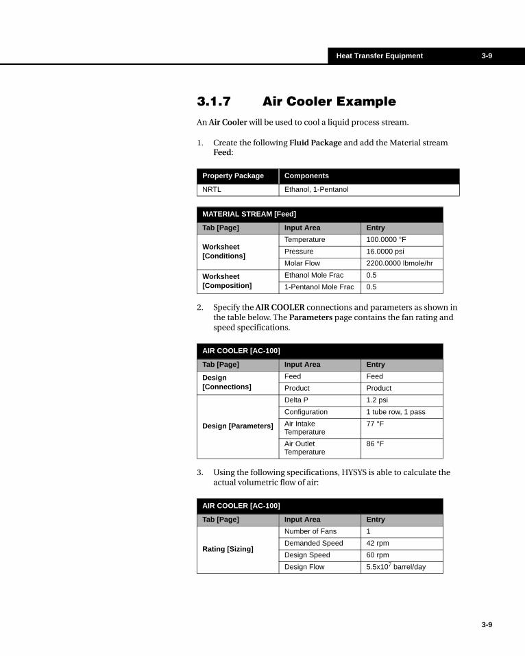
3.1.7 Air Cooler ExampleAn Air Cooler will be used to cool a liquid process stream.
1. Create the following Fluid Package and add the Material stream Feed:
2. Specify the AIR COOLER connections and parameters as shown in the table below. The Parameters page contains the fan rating and speed specifications.
3. Using the following specifications, HYSYS is able to calculate the actual volumetric flow of air:
Property Package Components
NRTL Ethanol, 1-Pentanol
MATERIAL STREAM [Feed]
Tab [Page] Input Area Entry
Worksheet [Conditions]
Temperature 100.0000 °F
Pressure 16.0000 psi
Molar Flow 2200.0000 lbmole/hr
Worksheet [Composition]
Ethanol Mole Frac 0.5
1-Pentanol Mole Frac 0.5
AIR COOLER [AC-100]
Tab [Page] Input Area Entry
Design [Connections]
Feed Feed
Product Product
Design [Parameters]
Delta P 1.2 psi
Configuration 1 tube row, 1 pass
Air Intake Temperature
77 °F
Air Outlet Temperature
86 °F
AIR COOLER [AC-100]
Tab [Page] Input Area Entry
Rating [Sizing]
Number of Fans 1
Demanded Speed 42 rpm
Design Speed 60 rpm
Design Flow 5.5x10⁷ barrel/day
3-9
3-10 Air Cooler
3-10
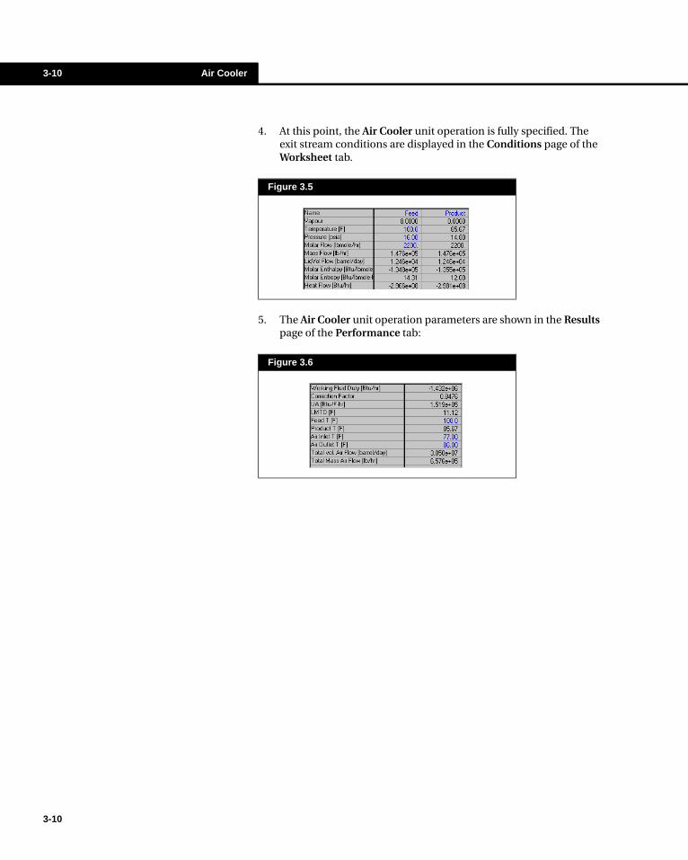
4. At this point, the Air Cooler unit operation is fully specified. The exit stream conditions are displayed in the Conditions page of the Worksheet tab.
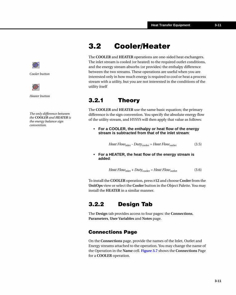
5. The Air Cooler unit operation parameters are shown in the Results page of the Performance tab:
Figure 3.5
Figure 3.6
Heat Transfer Equipment 3-11
3.2 Cooler/HeaterThe COOLER and HEATER operations are one-sided heat exchangers. The inlet stream is cooled (or heated) to the required outlet conditions, and the energy stream absorbs (or provides) the enthalpy difference between the two streams. These operations are useful when you are interested only in how much energy is required to cool or heat a process stream with a utility, but you are not interested in the conditions of the utility itself
3.2.1 TheoryThe COOLER and HEATER use the same basic equation; the primary difference is the sign convention. You specify the absolute energy flow of the utility stream, and HYSYS will then apply that value as follows:
• For a COOLER, the enthalpy or heat flow of the energy stream is subtracted from that of the inlet stream :
• For a HEATER, the heat flow of the energy stream is added :
To install the COOLER operation, press F12 and choose Cooler from the UnitOps view or select the Cooler button in the Object Palette. You may install the HEATER in a similar manner.
3.2.2 Design TabThe Design tab provides access to four pages: the Connections, Parameters, User Variables and Notes page.
Connections Page
On the Connections page, provide the names of the Inlet, Outlet and Energy streams attached to the operation. You may change the name of the Operation in the Name cell. Figure 3.7 shows the Connections Page for a COOLER operation.
Cooler button
Heater button
The only difference between the COOLER and HEATER is the energy balance sign convention.
Heat Flowinlet - Dutycooler = Heat Flowoutlet (3.5)
Heat Flowinlet + Dutycooler = Heat Flowoutlet (3.6)
3-11
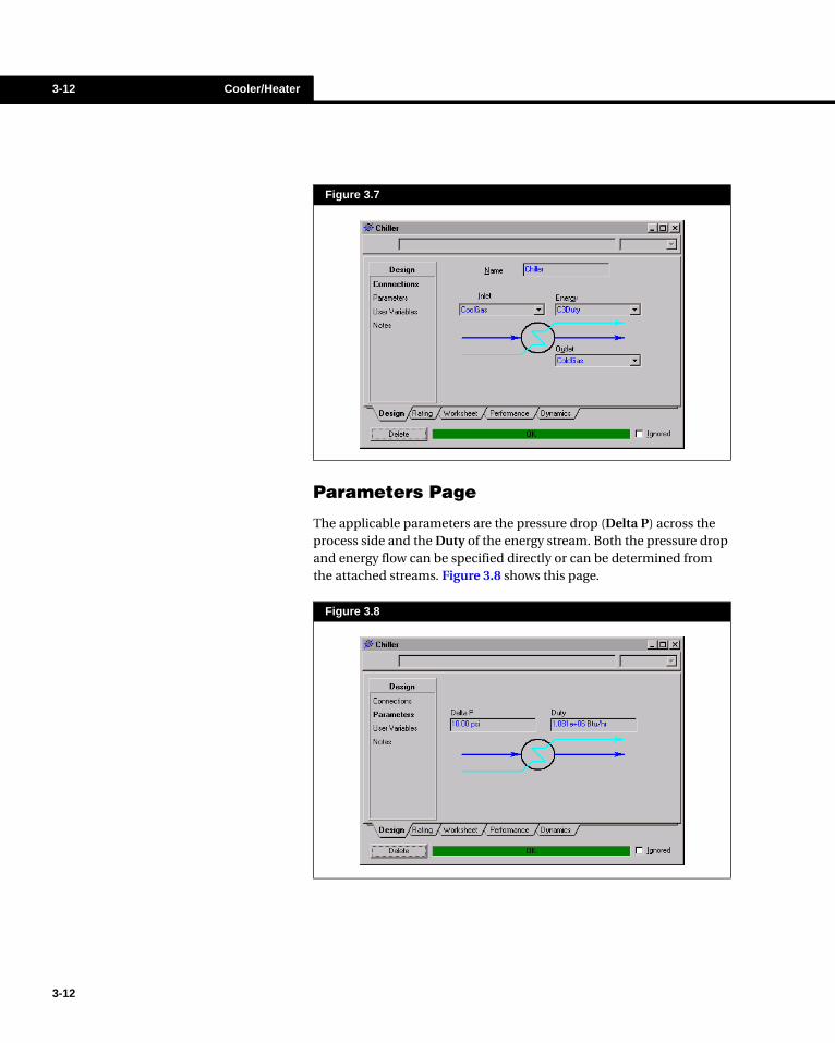
3-12 Cooler/Heater
3-12
Parameters Page
The applicable parameters are the pressure drop (Delta P) across the process side and the Duty of the energy stream. Both the pressure drop and energy flow can be specified directly or can be determined from the attached streams. Figure 3.8 shows this page.
Figure 3.7
Figure 3.8
Heat Transfer Equipment 3-13
You may supply a negative Duty value, however, be aware that:
• For a COOLER, a negative duty means that the unit is heating the inlet stream.
• For a HEATER, a negative duty means that the unit is cooling the inlet stream.
User Variables Page
The User Variables page allows you to attach code and customize your HYSYS simulation case by adding User Variables. For more information on implementing this option, see the User Variables chapter in the Customization Guide.
Notes Page
The Notes page provides an editor where you can record any remarks pertaining to the COOLER or HEATER or to your simulation case.
3.2.3 Rating Tab
Nozzles Page
On this page you are able to specify nozzle parameters on both the Inlet and Outlet streams connected to a COOLER or HEATER. Because the addition of nozzles to HEATERS and COOLERS is relevant when creating dynamic simulations, detailed information relating to this page is available in Chapter 4 - Heat Transfer Equipment of the Dynamics Modeling guide.
Heat Loss Page
Rating information regarding heat loss is relevant only in Dynamics mode. For information on specifying information on this page, see the Dynamic Modeling guide.
Remember that HYSYS will use the proper sign convention for the unit you have chosen, so you may always enter a positive duty value.
You are required to supply rating information only when working with a Dynamics simulation.
3-13

3-14 Cooler/Heater
3-14
3.2.4 Worksheet TabThe Worksheet tab contains a summary of the information contained in the stream property view for all the streams attached to the unit operation. The Conditions, Properties, and Composition pages contain selected information from the corresponding pages of the Worksheet tab for the stream property view. The PF Specs page contains a summary of the stream property view Dynamics tab.
3.2.5 Performance TabThe Performance tab contains pages that display calculated stream information. The performance parameters include the following stream properties:
• Pressure• Temperature• Vapour Fraction• Enthalpy
All information displayed on the Performance tab is read-only
Profiles Page
When viewing the Profiles page when working in Steady State, regardless of the number of zones specified, the Zone Conditions will be calculated for the Inlet zone only.
Figure 3.9
The PF Specs page is relevant to Dynamics cases only.
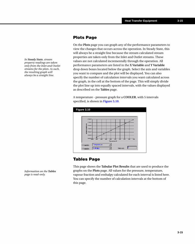
Heat Transfer Equipment 3-15
Plots Page
On the Plots page you can graph any of the performance parameters to view the changes that occurs across the operation. In Steady State, this will always be a straight line because the stream calculated stream properties are taken only from the Inlet and Outlet streams. These values are not calculated incrementally through the operation. All performance parameters are listed in the X Variable and Y Variable drop down boxes located below the graph. Select the axis and variables you want to compare and the plot will be displayed. You can also specify the number of calculation intervals you want calculated across the graph, in the cell at the bottom of the page. This will simply divide the plot line up into equally spaced intervals, with the values displayed as described on the Tables page.
A temperature - pressure graph for a COOLER, with 5 intervals specified, is shown in Figure 3.10.
Tables Page
This page shows the Tabular Plot Results that are used to produce the graphs on the Plots page. All values for the pressure, temperature, vapour fraction and enthalpy calculated for each interval is listed here. You can specify the number of calculation intervals at the bottom of this page.
Figure 3.10
In Steady State, stream property readings are taken only from the Inlet and Outlet streams for the plots. As such, the resulting graph will always be a straight line.
Information on the Tables page is read-only.
3-15

3-16 Cooler/Heater
3-16
3.2.6 Dynamics TabIf you are working exclusively in Steady State mode, you are not required to change any of the values on the pages accessible through this tab. For information on running the COOLER and HEATER operations in Dynamic mode, see the Dynamic Modeling guide, Chapter 4 - Heat Transfer Equipment for details.
3.2.7 Example - Gas CoolerA gas stream needs to be cooled from 60oF to -105oF with a pressure drop of 15 psi.
1. Create the following Fluid Package:
Figure 3.11
When working in Steady State mode, you are not required to change anything on this page.
Property Package Components
Peng Robinson Nitrogen, Carbon Dioxide, C1, C2, C3, i-C4, n-C4, i-C5, n-C5, n-C6, n-C7, n-C8

Heat Transfer Equipment 3-17
2. Install a material stream with the following specifications.
3. Install a COOLER, and complete the Connections page as shown in Figure 3.12.
4. Specify a Pressure Drop of 15 psi on the Parameters page.
5. Move to the Conditions page of the Worksheet tab. At this point, stream E-1 Outlet is not completely known, nor is the Duty value known. Use up the one degree of freedom remaining by specifying
MATERIAL STREAM [E-1 Inlet]
Tab [Page] Input Area Entry
Worksheet [Conditions]
Temperature 60.0000 F
Pressure 600.0000 psi
Molar Flow 100.0000 lbmole/hr
Worksheet [Composition]
Nitrogen Mole Frac 0.0149
CO2 Mole Frac 0.0020
Methane Mole Frac 0.9122
Ethane Mole Frac 0.0496
Propane Mole Frac 0.0148
i-Butane Mole Frac 0.0026
n-Butane Mole Frac 0.0020
i-Pentane Mole Frac 0.0010
n-Pentane Mole Frac 0.0006
n-Hexane Mole Frac 0.0001
n-Heptane Mole Frac 0.0001
n-Octane Mole Frac 0.0001
Figure 3.12Cooler Button
The duty required to cool stream E-1 Inlet to the conditions of E-1 Outlet is the Heat Flow of stream E-1 Duty. This duty will also be displayed on the Parameters page of the Design tab of the COOLER property view.
3-17
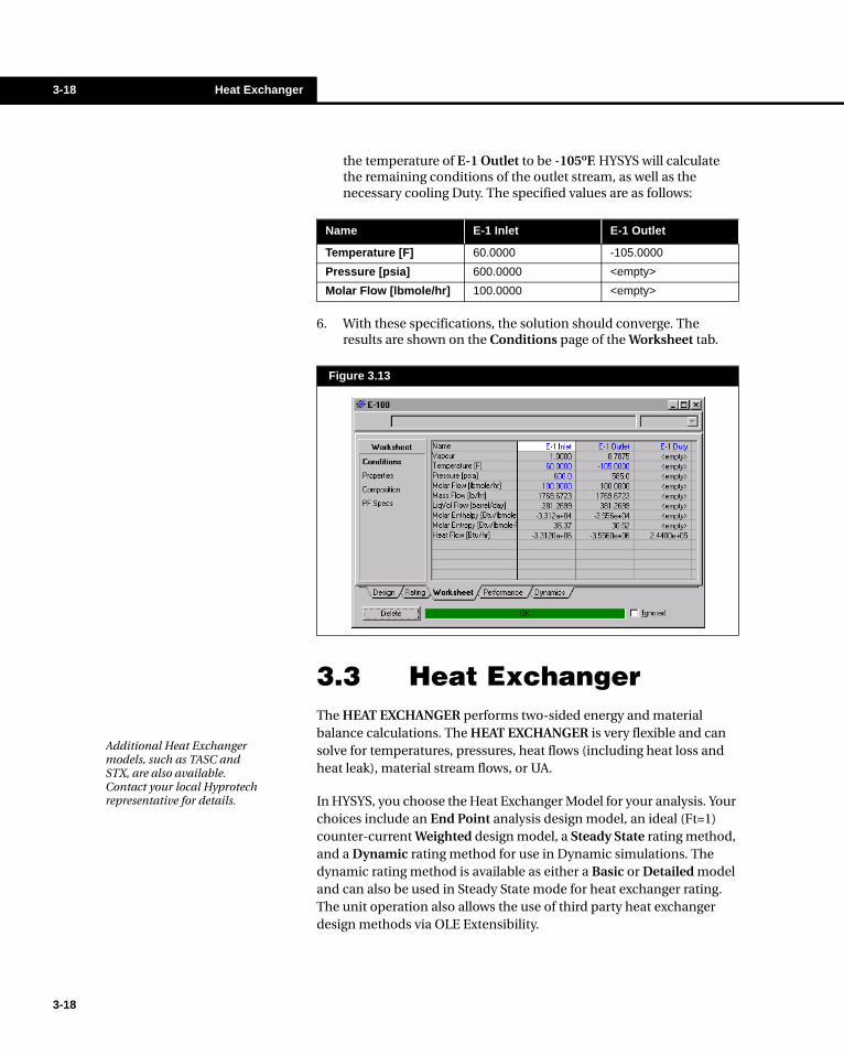
3-18 Heat Exchanger
3-18
the temperature of E-1 Outlet to be -105oF. HYSYS will calculate the remaining conditions of the outlet stream, as well as the necessary cooling Duty. The specified values are as follows:
6. With these specifications, the solution should converge. The results are shown on the Conditions page of the Worksheet tab.
3.3 Heat ExchangerThe HEAT EXCHANGER performs two-sided energy and material balance calculations. The HEAT EXCHANGER is very flexible and can solve for temperatures, pressures, heat flows (including heat loss and heat leak), material stream flows, or UA.
In HYSYS, you choose the Heat Exchanger Model for your analysis. Your choices include an End Point analysis design model, an ideal (Ft=1) counter-current Weighted design model, a Steady State rating method, and a Dynamic rating method for use in Dynamic simulations. The dynamic rating method is available as either a Basic or Detailed model and can also be used in Steady State mode for heat exchanger rating. The unit operation also allows the use of third party heat exchanger design methods via OLE Extensibility.
Name E-1 Inlet E-1 Outlet
Temperature [F] 60.0000 -105.0000
Pressure [psia] 600.0000 <empty>
Molar Flow [lbmole/hr] 100.0000 <empty>
Figure 3.13
Additional Heat Exchanger models, such as TASC and STX, are also available. Contact your local Hyprotech representative for details.
Heat Transfer Equipment 3-19
To install the HEAT EXCHANGER operation, press F12 and choose Heat Exchanger from the UnitOps view or select the Heat Exchanger button in the Object Palette.
To ignore the Heat Exchanger, select the Ignored check box. HYSYS will completely disregard the operation (and will not calculate the outlet stream) until you restore it to an active state by clearing the check box.
3.3.1 TheoryThe HEAT EXCHANGER calculations are based on energy balances for the hot and cold fluids. In the following general relations, the hot fluid supplies the heat exchanger duty to the cold fluid:
where: M = Fluid mass flow rate
H = Enthalpy
Qleak = Heat Leak
Qloss = Heat Loss
The Balance Error is a HEAT EXCHANGER Specification that will equal zero for most applications.
The subscripts hot and cold designate the hot and cold fluids, while in and out refer to the inlet and outlet.
The Heat Exchanger duty may also be defined in terms of the overall heat transfer coefficient, the area available for heat exchange and the log mean temperature difference:
where: U = Overall heat transfer coefficient
A = Surface area available for heat transfer
DTLM = Log mean temperature difference (LMTD)
Ft = LMTD correction factor
Note that the heat transfer coefficient and the surface area are often combined for convenience into a single variable referred to as UA. The LMTD and its correction factor are defined in the Performance section.
Heat Exchanger Button
(Mcold(Hout - Hin)cold - Qleak) - (Mhot(Hin - Hout)hot - Qloss) = Balance Error (3.7)
The HEAT EXCHANGER operation allows the heat curve for either side of the exchanger to be broken into intervals. Rather than calculating the energy transfer based on the terminal conditions of the exchanger, it is calculated for each of the intervals, then summed to determine the overall transfer.
Q = UADTLMFt (3.8)
3-19

3-20 Heat Exchanger
3-20
3.3.2 Design TabThe Design tab contains five pages: the Connections, Parameters, Specs, User Variables and Notes pages.
Connections Page
On the Connections page you provide the operation name as well as the names of the shell and tube inlet and outlet streams.
The Main Flowsheet is the default Flowsheet for the Tube and Shell side. You may select a Sub-Flowsheet on the Tube and/or Shell side which will allow you to choose inlet and outlet streams from that Flowsheet. This is useful for processes such as the Refrigeration cycle which require separate fluid packages for each side. You can define a Sub-Flowsheet with a different Fluid Package and then connect to the Main Flowsheet HEAT EXCHANGER.
Figure 3.14
Refer to the Heat Exchanger Example in Chapter 2 - Flowsheet Architecture for information on installing a HEAT EXCHANGER across Flowsheet boundaries.

Heat Transfer Equipment 3-21
Parameters Page
On the Parameters page, you can select the Heat Exchanger Model and specify relevant physical data. The Parameters page display depends on the Heat Exchanger Model selected.
From the drop down list, select the calculation model for the HEAT EXCHANGER. The following heat exchanger models are available:
• Exchanger Design (Endpoint)• Exchanger Design (Weighted)• Steady State Rating • Dynamic Rating
For both the Endpoint and Weighted design models you can specify whether your heat exchanger experiences heat loss. With this options there are two types of heat loss defined.
• Heat leak - Loss of cold side duty due to leakage. Duty gained to reflect the increase in temperature.
• Heat Loss - Loss of hot side duty due to leakage. Duty lost to reflect the decrease in temperature.
All Heat Exchanger models allow the specification of either Counter or Co-Current tube flow. See Section 3.3.3 - Rating Tab for further details.
End Point Design Model
The End Point exchanger design model is based on the standard heat exchanger duty equation (Equation (3.8)) defined in terms of overall heat transfer coefficient, area available for heat exchange and the log mean temperature difference. The main assumptions of the model are:
1. Overall heat transfer coefficient, U is constant.
2. Specific heats of both shell and tube side streams are constant.
Note that when a Heat Exchanger is installed as part of a Column Sub-Flowsheet (available when using the Modified HYSIM Inside-Out solving method) these Heat Exchanger Models are not available. Instead, in the Column Sub-Flowsheet, the Heat Exchanger is “Calculated from Column” as a simple heat and mass balance.
This section discusses the Steady State functioning of the Dynamic Rating heat exchanger. See the Dynamic Modeling guide, Chapter 4 - Heat Transfer Equipment for detailed information on the Dynamic Rating in Dynamics mode.
3-21
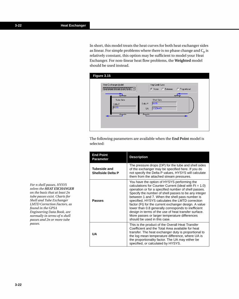
3-22 Heat Exchanger
3-22
In short, this model treats the heat curves for both heat exchanger sides as linear. For simple problems where there is no phase change and Cp is relatively constant, this option may be sufficient to model your Heat Exchanger. For non-linear heat flow problems, the Weighted model should be used instead.
The following parameters are available when the End Point model is selected:
Figure 3.15
End Point Parameter
Description
Tubeside and Shellside Delta P
The pressure drops (DP) for the tube and shell sides of the exchanger may be specified here. If you do not specify the Delta P values, HYSYS will calculate them from the attached stream pressures.
Passes
You have the option of HYSYS performing the calculations for Counter Current (ideal with Ft = 1.0) operation or for a specified number of shell passes. Specify the number of shell passes to be any integer between 1 and 7. When the shell pass number is specified, HYSYS calculates the LMTD correction factor (Ft) for the current exchanger design. A value lower than 0.8 generally corresponds to inefficient design in terms of the use of heat transfer surface. More passes or larger temperature differences should be used in this case.
UA
This is the product of the Overall Heat Transfer Coefficient and the Total Area available for heat transfer. The heat exchanger duty is proportional to the log mean temperature difference, where UA is the proportionality factor. The UA may either be specified, or calculated by HYSYS.
For n shell passes, HYSYS solves the HEAT EXCHANGER on the basis that at least 2n tube passes exist. Charts for Shell and Tube Exchanger LMTD Correction Factors, as found in the GPSA Engineering Data Book, are normally in terms of n shell passes and 2n or more tube passes.

Heat Transfer Equipment 3-23
Weighted Design Model
The Weighted exchanger design model is an excellent model to deal with non-linear heat curve problems such as the phase change of pure components in one or both heat exchanger sides. With the Weighted model, the heating curves are broken into intervals and an energy balance is performed along each interval. A LMTD and UA are calculated for each interval in the heat curve and summed to calculate the overall exchanger UA.
The Weighted model is available only for counter-current exchangers and is essentially an energy and material balance model. The geometry configurations which affect the Ft correction factor are not taken into consideration in this model.
When you select the Weighted model, the Parameters page will appear as shown in Figure 3.16.
The following table describes the items available on this page:
Figure 3.16
The Weighted Heat Exchanger Model is available for counter-current exchangers only.
Item Description
Heat Loss/Leak
You can specify whether or not there is heat loss/heat leak by choosing one of the radio buttons. By default, the None radio button is selected. The other two options incorporate heat loss/heat leak:
• Extremes - On the hot side, the heat is considered to be "lost" where the temperature is highest. Essentially, the top of the heat curve is being removed to allow for the heat loss/leak. This is the worst possible scenario. On the cold side, the heat is gained where the temperature is lowest.
• Proportional - The heat loss is distributed over all of the intervals.
3-23
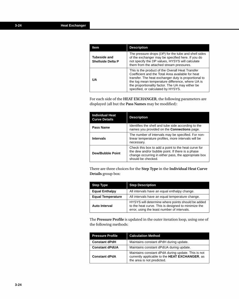
3-24 Heat Exchanger
3-24
For each side of the HEAT EXCHANGER, the following parameters are displayed (all but the Pass Names may be modified):
There are three choices for the Step Type in the Individual Heat Curve Details group box:
The Pressure Profile is updated in the outer iteration loop, using one of the following methods:
Tubeside and Shellside Delta P
The pressure drops (DP) for the tube and shell sides of the exchanger may be specified here. If you do not specify the DP values, HYSYS will calculate them from the attached stream pressures.
UA
This is the product of the Overall Heat Transfer Coefficient and the Total Area available for heat transfer. The heat exchanger duty is proportional to the log mean temperature difference, where UA is the proportionality factor. The UA may either be specified, or calculated by HYSYS.
Item Description
Individual Heat Curve Details
Description
Pass Name Identifies the shell and tube side according to the names you provided on the Connections page.
Intervals The number of intervals may be specified. For non-linear temperature profiles, more intervals will be necessary.
Dew/Bubble Point
Check this box to add a point to the heat curve for the dew and/or bubble point. If there is a phase change occurring in either pass, the appropriate box should be checked.
Step Type Step Description
Equal Enthalpy All intervals have an equal enthalpy change.
Equal Temperature All intervals have an equal temperature change.
Auto IntervalHYSYS will determine where points should be added to the heat curve. This is designed to minimize the error, using the least number of intervals.
Pressure Profile Calculation Method
Constant dPdH Maintains constant dPdH during update.
Constant dPdUA Maintains constant dPdUA during update.
Constant dPdAMaintains constant dPdA during update. This is not currently applicable to the HEAT EXCHANGER, as the area is not predicted.
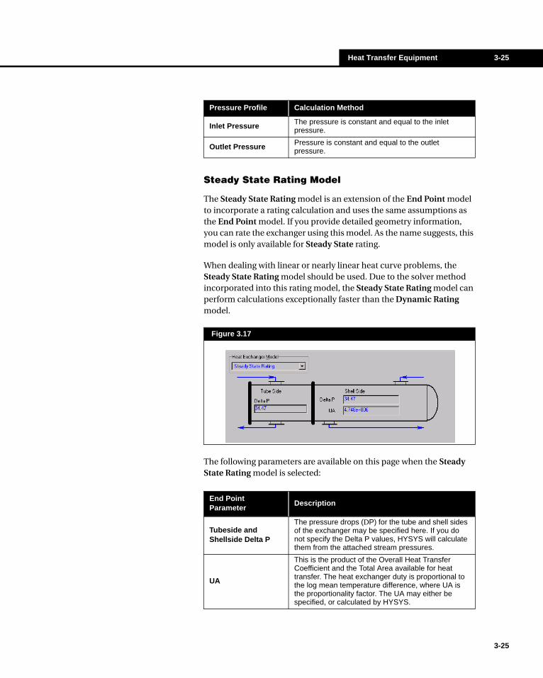
Heat Transfer Equipment 3-25
Steady State Rating Model
The Steady State Rating model is an extension of the End Point model to incorporate a rating calculation and uses the same assumptions as the End Point model. If you provide detailed geometry information, you can rate the exchanger using this model. As the name suggests, this model is only available for Steady State rating.
When dealing with linear or nearly linear heat curve problems, the Steady State Rating model should be used. Due to the solver method incorporated into this rating model, the Steady State Rating model can perform calculations exceptionally faster than the Dynamic Rating model.
The following parameters are available on this page when the Steady State Rating model is selected:
Inlet Pressure The pressure is constant and equal to the inlet pressure.
Outlet Pressure Pressure is constant and equal to the outlet pressure.
Pressure Profile Calculation Method
Figure 3.17
End Point Parameter
Description
Tubeside and Shellside Delta P
The pressure drops (DP) for the tube and shell sides of the exchanger may be specified here. If you do not specify the Delta P values, HYSYS will calculate them from the attached stream pressures.
UA
This is the product of the Overall Heat Transfer Coefficient and the Total Area available for heat transfer. The heat exchanger duty is proportional to the log mean temperature difference, where UA is the proportionality factor. The UA may either be specified, or calculated by HYSYS.
3-25

3-26 Heat Exchanger
3-26
Dynamic Rating
Two models are available for Dynamic Rating using the HEAT EXCHANGER unit operation: a Basic and a Detailed model. If you specify three temperatures or two temperatures and a UA, you can rate the exchanger with the Basic model. If you provide detailed geometry information, you can rate the exchanger using the Detailed model. Note that the Specs page will no longer appear when Dynamic Rating is selected.
The Basic model is based on the same assumptions as the End Point design model which uses the standard heat exchanger duty equation (Equation (3.8)) defined in terms of overall heat transfer coefficient, area available for heat exchange, and the log mean temperature difference. The Basic model is actually the counterpart of the End Point design model for Dynamics and dynamic rating but can also be used for Steady State heat exchanger rating.
The Detailed model is based on the same assumptions as the Weighted design model and divides the heat exchanger into a number of heat zones, performing an energy balance along each interval. This model requires detailed geometry information about your heat exchanger. The Detailed model is actually the counterpart of the Weighted design model for Dynamics and dynamic rating but can also be used for Steady State heat exchanger rating.
Once Dynamic Rating is selected, no further information is required from the Parameters page of the Design tab. Choice of Basic or Detailed model is made on the Parameters page of the Rating tab.
Figure 3.18

Heat Transfer Equipment 3-27
3-27
Specs Page
On the Specs page, you will find three group boxes that organize the various specification and solver information. The information provided in the Specs page is only valid for the Weighted, Endpoint and Steady State Rating models. This page will not appear when the Dynamic Rating model is selected
Solver Group
The following parameters are listed in the Solver group box:
Unknown Variables Group
HYSYS lists all unknown HEAT EXCHANGER variables according to your specified input. Once the unit has solved, the values of these variables will be displayed.
Specifications Group
Note that the Heat Balance (specified at 0 kJ/h) is considered to be a constraint. This is a Duty Error spec which you cannot turn off.
Figure 3.19
If you are working with a Dynamic Rating model, this page will not appear on the Design tab.
Solver Parameters Details
Tolerance The calculation error tolerance can be set.
Current ErrorWhen the current error is less than the calculation tolerance, the solution is considered to have converged.
Iterations
The current iteration of the outer loop is displayed. In the outer loop, the heat curve is updated and the property package calculations are performed. Non-rigorous property calculations are performed in the inner loop. Any constraints are also considered in the inner loop.
Without the Heat Balance specification, the heat equation will not balance. For this reason it is considered a Heat Exchanger constraint.
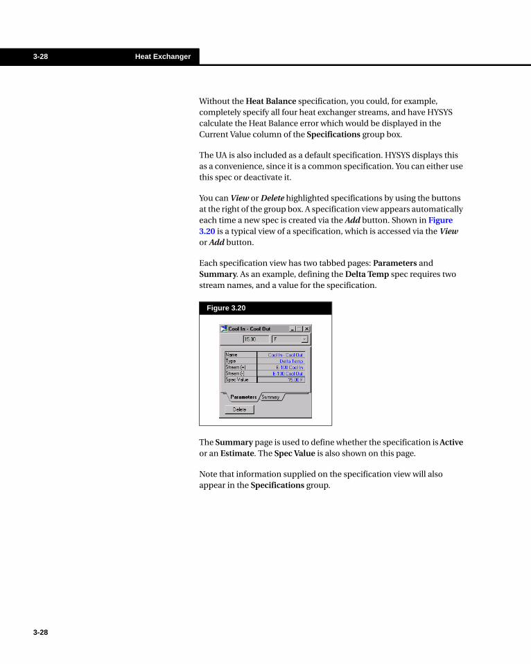
3-28 Heat Exchanger
3-28
Without the Heat Balance specification, you could, for example, completely specify all four heat exchanger streams, and have HYSYS calculate the Heat Balance error which would be displayed in the Current Value column of the Specifications group box.
The UA is also included as a default specification. HYSYS displays this as a convenience, since it is a common specification. You can either use this spec or deactivate it.
You can View or Delete highlighted specifications by using the buttons at the right of the group box. A specification view appears automatically each time a new spec is created via the Add button. Shown in Figure 3.20 is a typical view of a specification, which is accessed via the View or Add button.
Each specification view has two tabbed pages: Parameters and Summary. As an example, defining the Delta Temp spec requires two stream names, and a value for the specification.
The Summary page is used to define whether the specification is Active or an Estimate. The Spec Value is also shown on this page.
Note that information supplied on the specification view will also appear in the Specifications group.
Figure 3.20

Heat Transfer Equipment 3-29
All specifications will be one of the following three types:
The specification list allows you to try different combinations of the above three specification types. For example, suppose you have a number of specifications and you wish to determine which ones should be active, which should be estimates and which ones should be ignored altogether. By manipulating the check boxes among various specifications, you can test various combinations of the three types to see their effect on the results.
The available specification types include:
Specification Type Description
Active
An active specification is one that the convergence algorithm is trying to meet. Note that an active specification always serves as an initial estimate (when the Active box is checked, HYSYS automatically checks the Estimate box). An active specification exhausts one degree of freedom.
Estimate
An Estimate is considered an Inactive specification because the convergence algorithm is not trying to satisfy it. To use a specification as an estimate only, clear the Active check box. The value will then serve only as an initial estimate for the convergence algorithm. An estimate does not use an available degree of freedom.
Completely Inactive
To disregard the value of a specification entirely during convergence, clear both the Active and Estimate check boxes. By ignoring rather than deleting a specification, it will be available if you wish to use it later.
An Active specification is one that the convergence algorithm is trying to meet. An Active specification is on when both check boxes are selected.
An Estimate is used as an initial “guess” for the convergence algorithm, and is considered to be an inactive specification.
A Completely Inactive specification is one that is ignored completely by the convergence algorithm, but may be made Active or an Estimate at a later time.
Specification Description
TemperatureThe temperature of any stream attached to the HEAT EXCHANGER. The hot or cold inlet equilibrium temperature may also be defined.
Delta Temp
The temperature difference at the inlet or outlet between any two streams attached to the HEAT EXCHANGER. The hot or cold inlet equilibrium temperatures (which incorporate the heat loss/heat leak with the inlet conditions) may also be used.
Minimum Approach
Minimum internal temperature approach. The minimum temperature difference between the hot and cold stream (not necessarily at the inlet or outlet)
UA The overall UA (product of overall heat transfer coefficient and heat transfer area).
LMTD The overall log mean temperature difference.
The Hot Inlet Equilibrium temperature is the temperature of the inlet hot stream minus the heat loss temperature drop.
The Cold Inlet Equilibrium temperature is the temperature of the inlet cold stream plus the heat leak temperature rise.
3-29
3-30 Heat Exchanger
3-30
User Variables Page
The User Variables page allows you to attach code and customize your HYSYS simulation case by adding User Variables. For more information on implementing this option, see the User Variables chapter in the Customization Guide.
Notes Pages
The Notes page provides a text editor where you can record any comments or information regarding the HEAT EXCHANGER or pertaining to your simulation, in general.
3.3.3 Rating TabThe Rating tab contains four pages: the Sizing, Parameters, Nozzles and Heat Loss pages. The Parameters page is used exclusively by the Dynamics Heat Exchanger Model and will only become active either in Dynamics mode or while using the Dynamic Rating model.
Sizing Page
The Sizing page provides heat exchanger sizing related information. Based on the geometry information, HYSYS is able to calculate the pressure drop and the convective heat transfer coefficients for both heat exchanger sides and rate the exchanger.
The information is organized by three radio buttons: Overall, Shell, and Tube.
Duty
The overall duty, duty error, heat leak or heat loss. The duty error should normally be specified as 0 so that the heat balance will be satisfied. The heat leak and heat loss are available as specifications only if Heat Loss/Leak is set to Extremes or Proportional on the Parameters page.
Duty Ratio A duty ratio may be specified between any two of the following duties: overall, error, heat loss and heat leak.
Flow The flowrate of any attached stream (molar, mass or liquid volume).
Flow Ratio
The ratio of the two inlet stream flowrates. All other ratios are either impossible or redundant (i.e. - the inlet and outlet flowrates on the shell or tube side are equal).
Specification Description
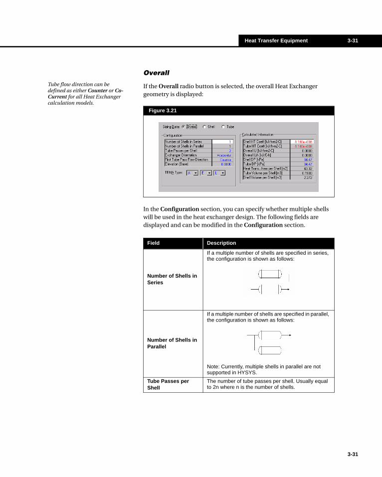
Heat Transfer Equipment 3-31
Overall
If the Overall radio button is selected, the overall Heat Exchanger geometry is displayed:
In the Configuration section, you can specify whether multiple shells will be used in the heat exchanger design. The following fields are displayed and can be modified in the Configuration section.
Figure 3.21
Tube flow direction can be defined as either Counter or Co-Current for all Heat Exchanger calculation models.
Field Description
Number of Shells in Series
If a multiple number of shells are specified in series, the configuration is shown as follows:
Number of Shells in Parallel
If a multiple number of shells are specified in parallel, the configuration is shown as follows:
Note: Currently, multiple shells in parallel are not supported in HYSYS.
Tube Passes per Shell
The number of tube passes per shell. Usually equal to 2n where n is the number of shells.
3-31
3-32 Heat Exchanger
3-32
You may specify the number of shell and tube passes in the shell of the heat exchanger. In general, at least 2n tube passes must be specified for every n shell pass. The exception is a counter-current flow heat exchanger which has 1 shell pass and one tube pass. The orientation may be specified as a vertical or horizontal heat exchanger. The orientation of the heat exchanger does not impact the steady state solver. However, it is used in the Dynamics Heat Exchanger Model in the calculation of liquid level in the shell.
The shape of Heat Exchanger may be specified using the TEMA-style drop down lists. The first list contains a list of front end stationary head types of the Heat Exchanger. The second list contains a list of shell types. The third list contains a list of rear end head types. For a more detailed discussion of TEMA-style shell-and-tube heat exchangers, refer to page 11-33 of the Perry’s Chemical Engineers’ Handbook (1997 edition).
In the Calculated Information group, the following heat exchanger parameters are listed:
• Shell HT Coeff• Tube HT Coeff• Overall U• Overall UA• Shell DP• Tube DP• Heat Trans. Area per Shell• Tube Volume per Shell• Shell Volume per Shell
Exchanger Orientation
The exchanger orientation defines whether or not the shell is horizontal or vertical. Used only in dynamic simulations.
When the shell orientation is vertical, you can also specify whether the shell feed is at the top or bottom via a checkbox:
First Tube Pass Flow Direction
Specifies whether or not the tube feed is co-current or counter-current.
Elevation (base) The height of the base of the exchanger above the ground. Used only in dynamic simulations.
Field Description
TEMA Type Drop down Lists
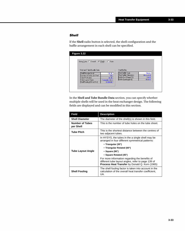
Heat Transfer Equipment 3-33
Shell
If the Shell radio button is selected, the shell configuration and the baffle arrangement in each shell can be specified.
In the Shell and Tube Bundle Data section, you can specify whether multiple shells will be used in the heat exchanger design. The following fields are displayed and can be modified in this section.
Figure 3.22
Field Description
Shell Diameter The diameter of the shell(s) is shown in this field.
Number of Tubes per Shell
This is the number of tube holes on the tube sheet.
Tube Pitch This is the shortest distance between the centres of two adjacent tubes.
Tube Layout Angle
In HYSYS, the tubes in the a single shell may be arranged in four different symmetrical patterns:
• Triangular (30°)
• Triangular Rotated (60°)
• Square (90°)
• Square Rotated (45°)
For more information regarding the benefits of different tube layout angles, refer to page 139 of Process Heat Transfer by Donald Q. Kern (1965)
Shell FoulingThe shell fouling factor is taken into account in the calculation of the overall heat transfer coefficient, UA.
3-33

3-34 Heat Exchanger
3-34
The following fields are displayed and can be modified in the Shell Baffles section:
Tube
If the Tube radio button is selected, information about the tube geometry in each shell can be specified:
In the Dimensions group, the following tube geometric parameters may be specified:
Field Description
Shell Baffle Type
You can choose 4 different baffle types:
• Single• Double• Triple• Grid
Shell Baffle Orientation
You can choose whether the baffles are aligned horizontally or vertically along the inner shell wall.
Baffle cut (Area%) You can specify the percent area the baffle occupies relative to the cross sectional area of the shell.
Baffle Spacing You can specify the space between each baffle.
Figure 3.23
Field Description
Outer Tube Diameter (OD)
Inner Tube Diameter (ID)
Tube Thickness
Two of the three listed parameters must be specified to characterize the tube width dimensions.
Tube LengthThis is the heat transfer length of one tube in a single heat exchanger shell. Note that this value is not the actual tube length.

Heat Transfer Equipment 3-35
In the Tube Properties group, the following metal tube heat transfer properties must be specified:
• Tube Fouling Factor• Thermal Conductivity• Wall Specific Heat Capacity, Cp• Wall Density
Parameters Page
The Parameters page of the Rating tab is used to define rating parameters for the Dynamic Rating model or the Dynamics Heat Exchanger Model. On the Parameters page, you can specify either a Basic model or a Detailed model. For the Basic model, you must define the Heat Exchanger’s overall UA and pressure drop across the shell and tube. For the Detailed model, you must define the geometry and heat transfer parameters of both the shell and tube sides in the Heat Exchanger operation. In order for either the Basic or Detailed Heat Exchanger Model to completely solve, the Parameters page must be completed.
Basic Model
Selecting the Basic model radio button on the Parameters page in Dynamics mode will bring up the following view:
Figure 3.24
3-35

3-36 Heat Exchanger
3-36
The Dimensions section contains the following information:
• Tube Volume• Shell Volume• Elevation (Base)
The tube volume, shell volume, and heat transfer area are calculated from Shell and Tube properties specified by selecting the Shell and Tube radio buttons on the Sizing page. The elevation of the base of the heat exchanger may be specified but does not impact the steady state solver.
The Parameters section includes the following Heat Exchanger parameters. All but the correction factor, F, may be modified:
Detailed Model
The Detailed model option allows you to specify the Zone Information, Heat Transfer Coefficient, and DeltaP details. Selecting the Detailed model radio button on the Parameters page will bring up the following view shown in Figure 3.25.
Field Description
Overall UA
This is the product of the Overall Heat Transfer Coefficient and the Total Area available for heat transfer. The heat exchanger duty is proportional to the log mean temperature difference, where UA is the proportionality factor. The UA may either be specified, or calculated by HYSYS.
Tubeside and Shellside Delta P
The pressure drops (DP) for the tube and shell sides of the exchanger may be specified here. If you do not specify the DP values, HYSYS will calculate them from the attached stream pressures.

Heat Transfer Equipment 3-37
Zone Information
HYSYS can partition the HEAT EXCHANGER into discrete multiple sections called zones. Because shell and tube stream conditions do not remain constant across the operation, the heat transfer parameters are not the same along the length of the heat exchanger. By dividing the heat exchanger into zones, you can make different heat transfer specifications for individual zones and therefore more accurately model an actual heat exchanger.
In the Zone Information section you can specify:
Figure 3.25
Field Description
Zones per Shell Pass
Enter the number of zones you would like for one shell. The total number of zones in a heat exchanger shell is calculated as:
Zone Fraction
The zone fraction is the fraction of space the zone occupies relative to the total shell volume. HYSYS automatically sets each zone to have the same volume. You may modify the zone fractions to occupy a larger or smaller proportion of the total volume. Press the Normalize Zone Fractions button in order to adjust the sum of fractions to equal one.
Total Zones Total Shell Passes Zones⋅=
3-37
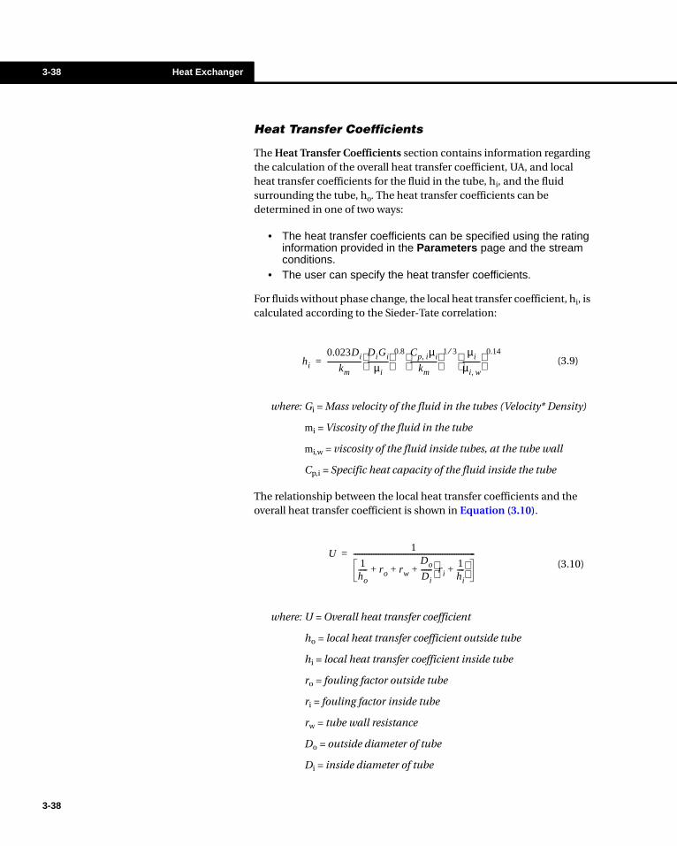
3-38 Heat Exchanger
3-38
Heat Transfer Coefficients
The Heat Transfer Coefficients section contains information regarding the calculation of the overall heat transfer coefficient, UA, and local heat transfer coefficients for the fluid in the tube, hi, and the fluid surrounding the tube, ho. The heat transfer coefficients can be determined in one of two ways:
• The heat transfer coefficients can be specified using the rating information provided in the Parameters page and the stream conditions.
• The user can specify the heat transfer coefficients.
For fluids without phase change, the local heat transfer coefficient, hi, is calculated according to the Sieder-Tate correlation:
where: Gi = Mass velocity of the fluid in the tubes (Velocity* Density)
mi = Viscosity of the fluid in the tube
mi,w = viscosity of the fluid inside tubes, at the tube wall
Cp,i = Specific heat capacity of the fluid inside the tube
The relationship between the local heat transfer coefficients and the overall heat transfer coefficient is shown in Equation (3.10).
where: U = Overall heat transfer coefficient
ho = local heat transfer coefficient outside tube
hi = local heat transfer coefficient inside tube
ro = fouling factor outside tube
ri = fouling factor inside tube
rw = tube wall resistance
Do = outside diameter of tube
Di = inside diameter of tube
(3.9)hi
0.023Di
km-------------------
DiGi
µi------------
0.8 Cp i, µi
km---------------
1 3⁄ µi
µi w,----------
0.14=
(3.10)U
1
1ho----- ro rw
Do
Di------ ri
1hi----+
+ + +
---------------------------------------------------------------------=
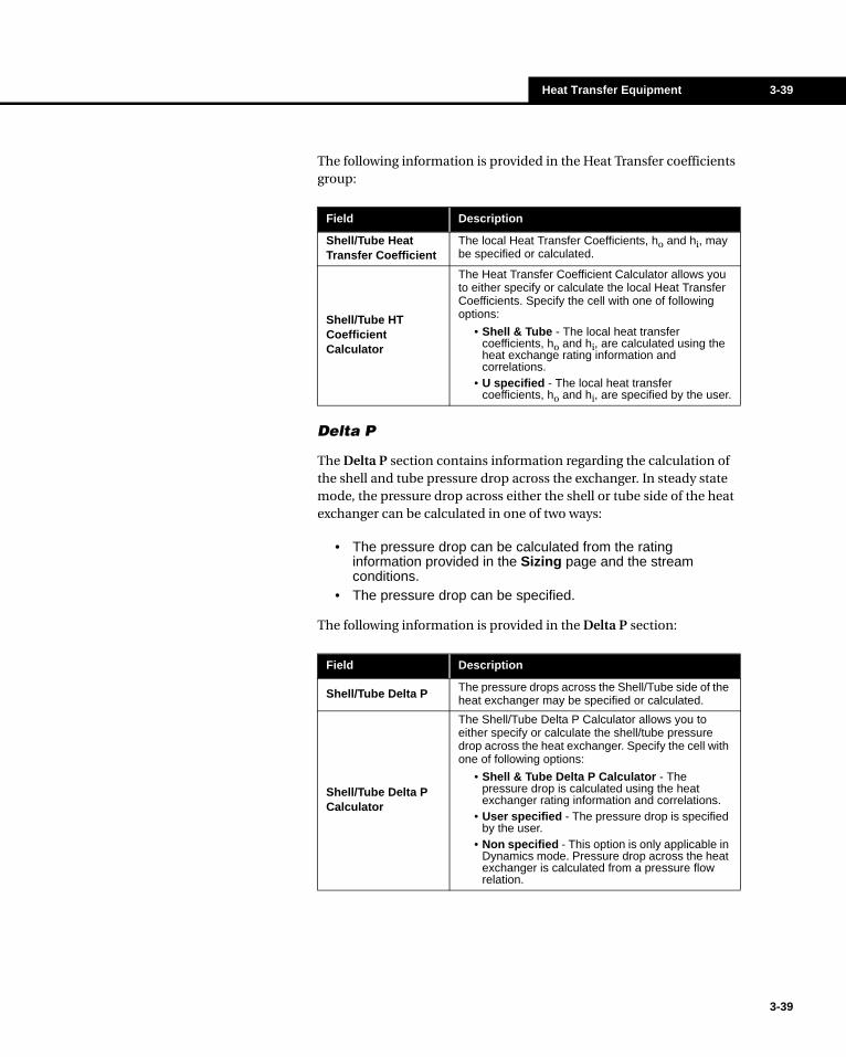
Heat Transfer Equipment 3-39
The following information is provided in the Heat Transfer coefficients group:
Delta P
The Delta P section contains information regarding the calculation of the shell and tube pressure drop across the exchanger. In steady state mode, the pressure drop across either the shell or tube side of the heat exchanger can be calculated in one of two ways:
• The pressure drop can be calculated from the rating information provided in the Sizing page and the stream conditions.
• The pressure drop can be specified.
The following information is provided in the Delta P section:
Field Description
Shell/Tube Heat Transfer Coefficient
The local Heat Transfer Coefficients, ho and hi, may be specified or calculated.
Shell/Tube HT Coefficient Calculator
The Heat Transfer Coefficient Calculator allows you to either specify or calculate the local Heat Transfer Coefficients. Specify the cell with one of following options:
• Shell & Tube - The local heat transfer coefficients, ho and hi, are calculated using the heat exchange rating information and correlations.
• U specified - The local heat transfer coefficients, ho and hi, are specified by the user.
Field Description
Shell/Tube Delta P The pressure drops across the Shell/Tube side of the heat exchanger may be specified or calculated.
Shell/Tube Delta P Calculator
The Shell/Tube Delta P Calculator allows you to either specify or calculate the shell/tube pressure drop across the heat exchanger. Specify the cell with one of following options:
• Shell & Tube Delta P Calculator - The pressure drop is calculated using the heat exchanger rating information and correlations.
• User specified - The pressure drop is specified by the user.
• Non specified - This option is only applicable in Dynamics mode. Pressure drop across the heat exchanger is calculated from a pressure flow relation.
3-39
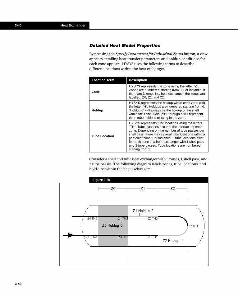
3-40 Heat Exchanger
3-40
Detailed Heat Model Properties
By pressing the Specify Parameters for Individual Zones button, a view appears detailing heat transfer parameters and holdup conditions for each zone appears. HYSYS uses the following terms to describe different locations within the heat exchanger.
Consider a shell and tube heat exchanger with 3 zones, 1 shell pass, and 2 tube passes. The following diagram labels zones, tube locations, and hold-ups within the heat exchanger:
Location Term Description
Zone
HYSYS represents the zone using the letter “Z”. Zones are numbered starting from 0. For instance, if there are 3 zones in a heat exchanger, the zones are labelled: Z0, Z1, and Z2.
Holdup
HYSYS represents the holdup within each zone with the letter “H”. Holdups are numbered starting from 0. “Holdup 0” will always be the holdup of the shell within the zone. Holdups 1 through n will represent the n tube holdups existing in the zone.
Tube Location
HYSYS represents tube locations using the letters “TH”. Tube locations occur at the interface of each zone. Depending on the number of tube passes per shell pass, there may several tube locations within a particular zone. For instance, 2 tube locations exist for each zone in a heat exchanger with 1 shell pass and 2 tube passes. Tube locations are numbered starting from 1.
Figure 3.26
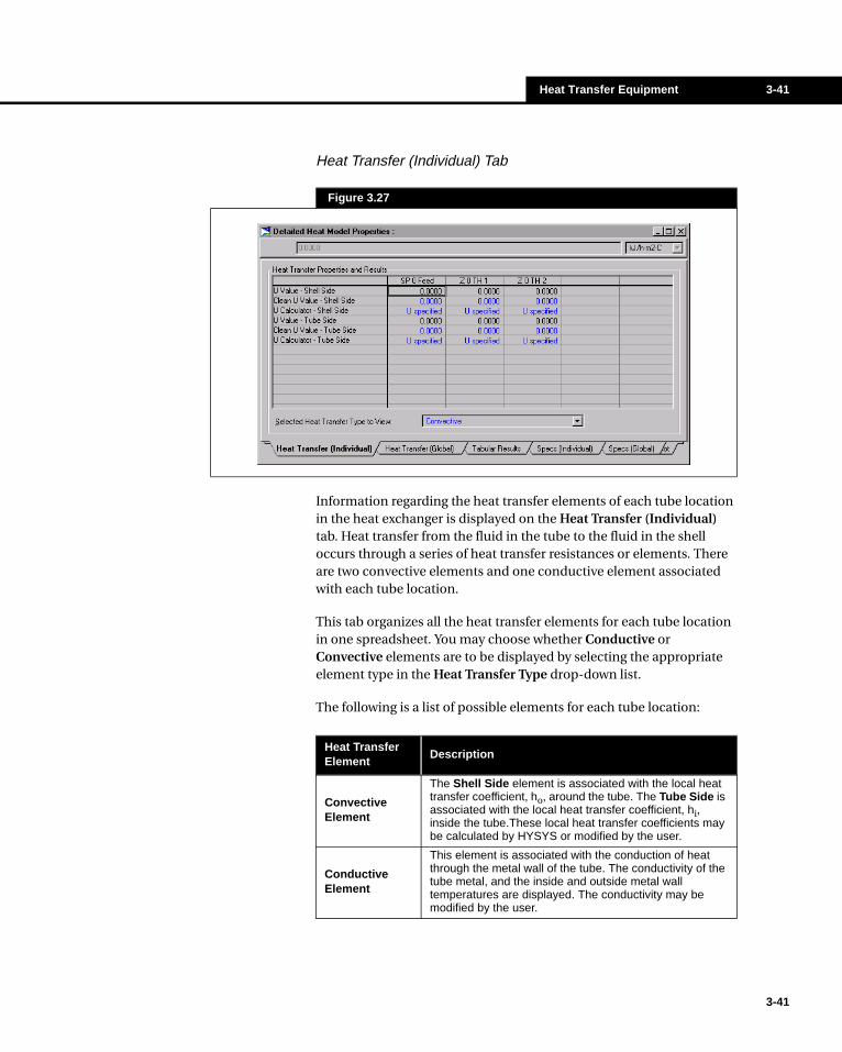
Heat Transfer Equipment 3-41
Heat Transfer (Individual) Tab
Information regarding the heat transfer elements of each tube location in the heat exchanger is displayed on the Heat Transfer (Individual) tab. Heat transfer from the fluid in the tube to the fluid in the shell occurs through a series of heat transfer resistances or elements. There are two convective elements and one conductive element associated with each tube location.
This tab organizes all the heat transfer elements for each tube location in one spreadsheet. You may choose whether Conductive or Convective elements are to be displayed by selecting the appropriate element type in the Heat Transfer Type drop-down list.
The following is a list of possible elements for each tube location:
Figure 3.27
Heat Transfer Element
Description
Convective Element
The Shell Side element is associated with the local heat transfer coefficient, ho, around the tube. The Tube Side is associated with the local heat transfer coefficient, hi, inside the tube.These local heat transfer coefficients may be calculated by HYSYS or modified by the user.
Conductive Element
This element is associated with the conduction of heat through the metal wall of the tube. The conductivity of the tube metal, and the inside and outside metal wall temperatures are displayed. The conductivity may be modified by the user.
3-41
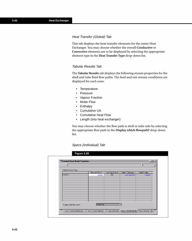
3-42 Heat Exchanger
3-42
Heat Transfer (Global) Tab
This tab displays the heat transfer elements for the entire Heat Exchanger. You may choose whether the overall Conductive or Convective elements are to be displayed by selecting the appropriate element type in the Heat Transfer Type drop-down list.
Tabular Results Tab
The Tabular Results tab displays the following stream properties for the shell and tube fluid flow paths. The feed and exit stream conditions are displayed for each zone.
• Temperature• Pressure• Vapour Fraction• Molar Flow• Enthalpy• Cumulative UA• Cumulative Heat Flow• Length (into heat exchanger)
You may choose whether the flow path is shell or tube side by selecting the appropriate flow path in the Display which flowpath? drop-down list.
Specs (Individual) Tab
Figure 3.28
Heat Transfer Equipment 3-43
3-43
This tab displays the pressure drop specifications for each shell and tube holdup in one spreadsheet. The Pressure Flow K and Use Pressure Flow K columns are applicable only in Dynamics mode.
You may choose whether the shell or tube side is displayed by selecting the Display which flowpath? drop-down list.
Specs (Global) Tab
This tab displays the pressure drop specifications for the entire shell and tube holdups. The Pressure Flow K and Use Pressure Flow K columns are applicable only in Dynamics mode.
You may choose whether the shell or tube side is displayed by selecting the Display which flowpath? drop-down list.
Plots Tab
The information displayed in this tab is a graphical representation of the parameters provided in the Tabular Results tab. You can plot the following variables for the shell and tube side of the heat exchanger:
• Vapour Fraction• Molar Flow• Enthalpy• Cumulative UA• Heat Flow • Length
3.3.4 Worksheet TabThe Worksheet tab contains a summary of the information contained in the stream property view for all the streams attached to the Heat Exchanger unit operation. The Conditions, Properties, and Composition pages contain selected information from the corresponding pages of the Worksheet tab for the stream property view. The PF Specs page contains a summary of the stream property view Dynamics tab.
To see the stream parameters broken down per stream phase, open the Worksheet tab of the Stream Property View.
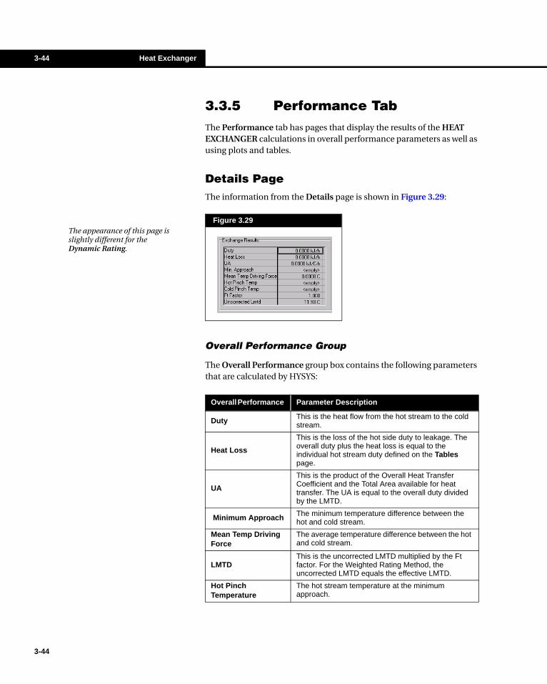
3-44 Heat Exchanger
3-44
3.3.5 Performance TabThe Performance tab has pages that display the results of the HEAT EXCHANGER calculations in overall performance parameters as well as using plots and tables.
Details PageThe information from the Details page is shown in Figure 3.29:
Overall Performance Group
The Overall Performance group box contains the following parameters that are calculated by HYSYS:
Figure 3.29The appearance of this page is slightly different for the Dynamic Rating.
Overall Performance Parameter Description
Duty This is the heat flow from the hot stream to the cold stream.
Heat Loss
This is the loss of the hot side duty to leakage. The overall duty plus the heat loss is equal to the individual hot stream duty defined on the Tables page.
UA
This is the product of the Overall Heat Transfer Coefficient and the Total Area available for heat transfer. The UA is equal to the overall duty divided by the LMTD.
Minimum Approach The minimum temperature difference between the hot and cold stream.
Mean Temp Driving Force
The average temperature difference between the hot and cold stream.
LMTD This is the uncorrected LMTD multiplied by the Ft factor. For the Weighted Rating Method, the uncorrected LMTD equals the effective LMTD.
Hot Pinch Temperature
The hot stream temperature at the minimum approach.
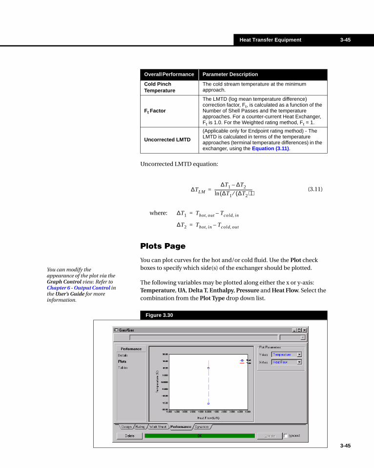
Heat Transfer Equipment 3-45
3-45
Uncorrected LMTD equation:
where:
Plots Page
You can plot curves for the hot and/or cold fluid. Use the Plot check boxes to specify which side(s) of the exchanger should be plotted.
The following variables may be plotted along either the x or y-axis: Temperature, UA, Delta T, Enthalpy, Pressure and Heat Flow. Select the combination from the Plot Type drop down list.
Cold Pinch Temperature
The cold stream temperature at the minimum approach.
Ft Factor
The LMTD (log mean temperature difference) correction factor, Ft, is calculated as a function of the Number of Shell Passes and the temperature approaches. For a counter-current Heat Exchanger, Ft is 1.0. For the Weighted rating method, Ft = 1.
Uncorrected LMTD
(Applicable only for Endpoint rating method) - The LMTD is calculated in terms of the temperature approaches (terminal temperature differences) in the exchanger, using the Equation (3.11).
Overall Performance Parameter Description
(3.11)∆TLM
∆T1 ∆T2–
∆T1 ∆T2( )⁄( )ln---------------------------------------=
∆T1 Thot out, Tcold in,–=
∆T2 Thot in, Tcold o, ut–=
You can modify the appearance of the plot via the Graph Control view. Refer to Chapter 6 - Output Control in the User’s Guide for more information.
Figure 3.30

3-46 Heat Exchanger
3-46
Tables Page
On the Tables page, you can view the interval Temperature, Pressure, Heat Flow, Enthalpy, UA and Vapour Fraction for each side of the Exchanger in a tabular format. Select either the Shell Side or Tube Side radio button.
3.3.6 Dynamics TabIf you are working exclusively in Steady State mode, you are not required to change any information on the pages accessible through this tab. Any information specified in the Rating tab is also displayed in the Dynamics tab. For more information on running the Heat Exchanger operations in Dynamics mode, see the Dynamic Modeling guide for further details.
3.3.7 Heat Exchanger ExamplesA simple water-water Heat Exchanger example is outlined in this section. There is an additional Heat Exchanger example in this manual and a further example in the User’s Guide, both of which are more advanced:
• An example of Multiple Heat Exchangers is shown in the Chapter 11 - Optimizer.
• Refer to the SubFlowsheet Refrigeration Cycle Example (Chapter 2 - Flowsheet Architecture in the User’s Guide ) to see how subflowsheets can be used within HEAT EXCHANGER.
1. In this example, the inlet streams are fully defined as follows (using the ASME Steam property method):
For detailed information on using HEAT EXCHANGERS in dynamics mode, see Chapter 4 - Heat Transfer Equipment in the Dynamic Modeling guide.
For Heat Exchanger Examples, see Chapter 11 - Optimizer in this manual and Chapter 2 - Flowsheet Architecture in the User’s Guide.
MATERIAL STREAM [Tube In]
Tab [Page] Input Area Entry
Worksheet [Conditions]
Temperature 120.0000 °F
Pressure 100.0000 psi
Molar Flow 5000.0000 lbmole/hr
Worksheet [Composition]
H2O Mole Frac 1.0000

Heat Transfer Equipment 3-47
2. The HEAT EXCHANGER connections are shown below:
3. On the Parameters page, enter Tube Side Delta P and Shell Side Delta P values of 5 psi.
4. Note that at this point, there is just one degree of freedom available. Specifying an outlet temperature on either side of the exchanger would result in the HEAT EXCHANGER having enough information to calculate. Select the Weighted rating method from the Heat Exchanger Model drop down list, and choose the Extremes radio button in the Heat Loss/Leak group. This increases the degrees of freedom to three, because specifications have to be supplied to account for the Heat Leak and Heat Loss.
MATERIAL STREAM [Shell In]
Tab [Page] Input Area Entry
Worksheet [Conditions]
Temperature 90.0000 °F
Pressure 100.0000 psi
Molar Flow 4000.0000 lbmole/hr
Worksheet [Composition]
H2O Mole Frac 1.0000
Figure 3.31
In order to incorporate Heat Loss/Leak, the Rating Method must be Weighted. When Heat Loss/Leak is set to Extremes, heat is "lost" on the hot side where the temperature is highest. Conversely, heat is "gained" on the cold side where temperature is lowest.
3-47
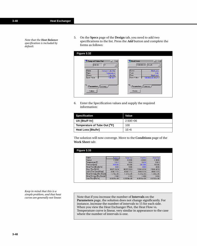
3-48 Heat Exchanger
3-48
5. On the Specs page of the Design tab, you need to add two specifications to the list. Press the Add button and complete the forms as follows:
6. Enter the Specification values and supply the required information:
The solution will now converge. Move to the Conditions page of the Work Sheet tab:
Figure 3.32
Note that the Heat Balance specification is included by default.
Specification Value
UA [Btu/F-hr] 2.50E+06
Temperature of Tube Out [oF] 100
Heat Loss [Btu/hr] 1E+6
Figure 3.33
Keep in mind that this is a simple problem, and that heat curves are generally not linear. Note that if you increase the number of Intervals on the
Parameters page, the solution does not change significantly. For instance, increase the number of intervals to 15 for each side. When you view the Heat Exchanger Plot, the Heat Flow vs. Temperature curve is linear, very similar in appearance to the case where the number of intervals is one.
Heat Transfer Equipment 3-49
3.4 Fired Heater (Furnace)This operation can only be used in dynamic mode. Refer Section 4.5 - Fired Heater (Furnace) of the Dynamic Modeling guide for information on this operation.
3.5 LNGThe LNG (Liquefied Natural Gas) exchanger model solves heat and material balances for multi-stream heat exchangers and heat exchanger networks. The solution method can handle a wide variety of specified and unknown variables.
For the overall exchanger, you can specify various parameters, including heat leak/heat loss, UA or temperature approaches. Two solution approaches are employed; in the case of a single unknown, the solution is calculated directly from an energy balance. In the case of multiple unknowns, an iterative approach is used which attempts to determine the solution which satisfies not only the energy balance, but any constraints, such as temperature approach or UA.
To install the LNG operation, press F12 and choose LNG or select the LNG Exchanger button in the Object Palette.
LNG Button
The LNG allows for multiple streams, while the HEAT EXCHANGER allows only one hot side stream and one cold side stream.
3-49

3-50 LNG
3-50
3.5.1 Design TabThere are five pages on the Design tab: Connections, Parameters, Specs, User Variables and Notes.
Connections Page
The Connections page is shown in the Figure 3.34.
For each exchanger side:
• An inlet stream and outlet stream are required.• A Pressure Drop is required.• The Hot/Cold designation can be specified. This will be used as
an estimate for calculations and will also be used for drawing the PFD. If a designated hot pass is actually cold (or vice versa), the operation will still solve properly. The actual Hot/Cold designation (as determined by the LNG) can be found on the Side Results page.
• The Main Flowsheet is the default shown in the Flowsheet column. Refer to the Heat Exchanger Example in Chapter 2 - Flowsheet Architecture in the User’s Guide to see how Sub-Flowsheets can be used in the Heat Exchanger or LNG.
Note that any number of Sides may be added simply by selecting the Add Side button. To remove a side, select the Delete Side button after positioning the cursor in the appropriate row.
Figure 3.34
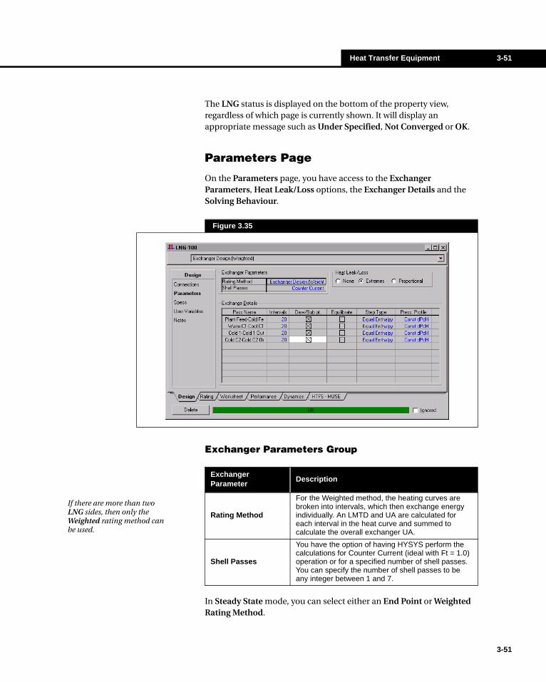
Heat Transfer Equipment 3-51
The LNG status is displayed on the bottom of the property view, regardless of which page is currently shown. It will display an appropriate message such as Under Specified, Not Converged or OK.
Parameters Page
On the Parameters page, you have access to the Exchanger Parameters, Heat Leak/Loss options, the Exchanger Details and the Solving Behaviour.
Exchanger Parameters Group
In Steady State mode, you can select either an End Point or Weighted Rating Method.
Figure 3.35
Exchanger Parameter
Description
Rating Method
For the Weighted method, the heating curves are broken into intervals, which then exchange energy individually. An LMTD and UA are calculated for each interval in the heat curve and summed to calculate the overall exchanger UA.
Shell Passes
You have the option of having HYSYS perform the calculations for Counter Current (ideal with Ft = 1.0) operation or for a specified number of shell passes. You can specify the number of shell passes to be any integer between 1 and 7.
If there are more than two LNG sides, then only the Weighted rating method can be used.
3-51

3-52 LNG
3-52
Heat Leak/Loss Group
By default, the None radio button is selected. The other two radio buttons incorporate heat loss/heat leak:
Note that Heat Loss/Leak options can be set only when the Rating Method is Weighted.
Exchange Details Group
The LNG Exchange Details are displayed as follows:
For each side, the following parameters may be specified:
Heat Loss Description
ExtremesThe heat loss and heat leak are considered to occur only at the end points (inlets and outlets) and are applied to the Hot and Cold Equilibrium streams.
Proportional The heat loss and heat leak will be applied over each interval.
Figure 3.36
Parameter Description
Intervals
The number of intervals, applicable only to the Weighted Rating Method, may be specified. For non-linear temperature profiles, more intervals will be necessary.
Dew/Bubble Point
Check this box to add a point to the Heat curve for a phase change. Figure 3.37 illustrates the effect of the number of intervals and inclusion of the dew and bubble points on the temperature / heat flow curves. Temperature is on the y-axis, and heat flow is on the x-axis
Equilibrate
All sides that are checked will come to thermal equilibrium before entering into the UA and LMTD calculations. If only one hot stream or cold stream is checked, then that stream is by definition in equilibrium with itself and the results will not be affected. If two or more hot or cold streams are checked, then the effective driving force will be reduced. All unchecked streams enter the composite curve at their respective temperatures.
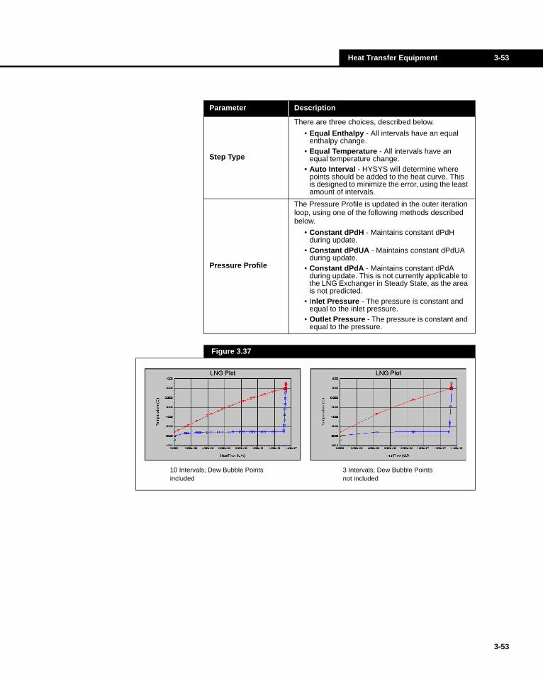
Heat Transfer Equipment 3-53
Step Type
There are three choices, described below.
• Equal Enthalpy - All intervals have an equal enthalpy change.
• Equal Temperature - All intervals have an equal temperature change.
• Auto Interval - HYSYS will determine where points should be added to the heat curve. This is designed to minimize the error, using the least amount of intervals.
Pressure Profile
The Pressure Profile is updated in the outer iteration loop, using one of the following methods described below.
• Constant dPdH - Maintains constant dPdH during update.
• Constant dPdUA - Maintains constant dPdUA during update.
• Constant dPdA - Maintains constant dPdA during update. This is not currently applicable to the LNG Exchanger in Steady State, as the area is not predicted.
• Inlet Pressure - The pressure is constant and equal to the inlet pressure.
• Outlet Pressure - The pressure is constant and equal to the pressure.
Figure 3.37
Parameter Description
10 Intervals; Dew Bubble Points included
3 Intervals; Dew Bubble Points not included
3-53

3-54 LNG
3-54
Specs Page
On the Specs page, you will find four group boxes which organize the various specification and solver information.
Solver Group
The Solver group box includes the solving parameters used for LNG’s:
Degrees of Freedom Group
To help reach the desired solution, unknown parameters (flows, temperatures) can be manipulated in the attached streams. Each parameter specification will reduce the Degrees of Freedom by one. The Degrees of Freedom value for the LNG is shown within the Solver group.
Figure 3.38
Solver Parameter Specification Description
Tolerance You may set the calculation error tolerance.
Current ErrorWhen the current error is less than the calculation tolerance, the solution is considered to have converged.
Iterations
The current iteration of the outer loop is displayed. In the outer loop, the heat curve is updated and the property package calculations are performed. Non-rigorous property calculations are performed in the inner loop. Any constraints are also considered in the inner loop.
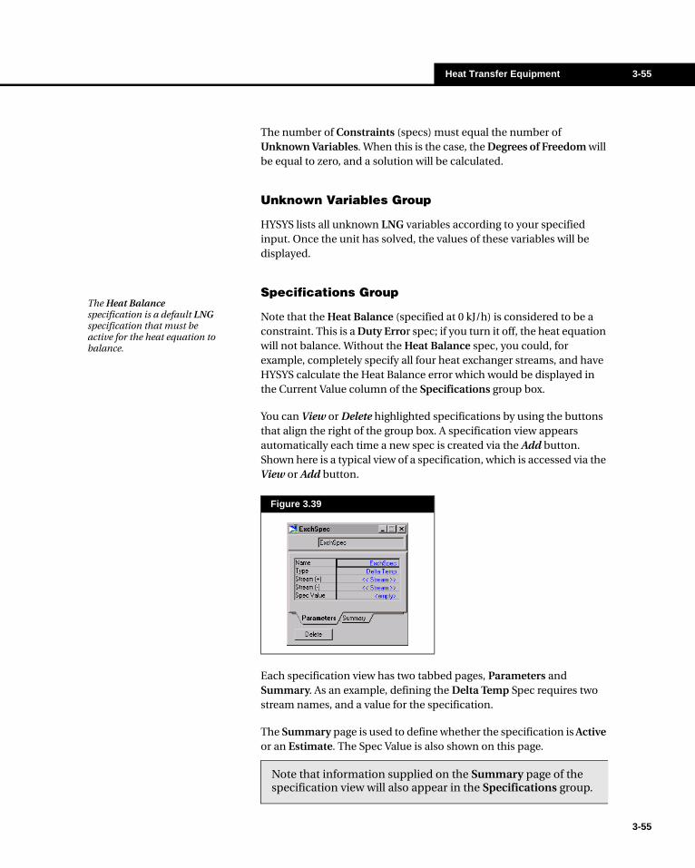
Heat Transfer Equipment 3-55
The number of Constraints (specs) must equal the number of Unknown Variables. When this is the case, the Degrees of Freedom will be equal to zero, and a solution will be calculated.
Unknown Variables Group
HYSYS lists all unknown LNG variables according to your specified input. Once the unit has solved, the values of these variables will be displayed.
Specifications Group
Note that the Heat Balance (specified at 0 kJ/h) is considered to be a constraint. This is a Duty Error spec; if you turn it off, the heat equation will not balance. Without the Heat Balance spec, you could, for example, completely specify all four heat exchanger streams, and have HYSYS calculate the Heat Balance error which would be displayed in the Current Value column of the Specifications group box.
You can View or Delete highlighted specifications by using the buttons that align the right of the group box. A specification view appears automatically each time a new spec is created via the Add button. Shown here is a typical view of a specification, which is accessed via the View or Add button.
Each specification view has two tabbed pages, Parameters and Summary. As an example, defining the Delta Temp Spec requires two stream names, and a value for the specification.
The Summary page is used to define whether the specification is Active or an Estimate. The Spec Value is also shown on this page.
Figure 3.39
The Heat Balance specification is a default LNG specification that must be active for the heat equation to balance.
Note that information supplied on the Summary page of the specification view will also appear in the Specifications group.
3-55
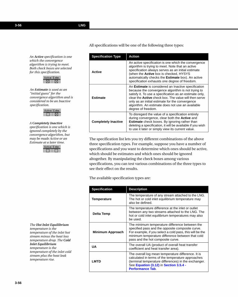
3-56 LNG
3-56
All specifications will be one of the following three types:
The specification list lets you try different combinations of the above three specification types. For example, suppose you have a number of specifications and you want to determine which ones should be active, which should be estimates and which ones should be ignored altogether. By manipulating the check boxes among various specifications, you can test various combinations of the three types to see their effect on the results.
The available specification types are:
Specification Type Action
Active
An active specification is one which the convergence algorithm is trying to meet. Note that an active specification always serves as an initial estimate (when the Active box is checked, HYSYS automatically checks the Estimate box). An active specification exhausts one degree of freedom.
Estimate
An Estimate is considered an Inactive specification because the convergence algorithm is not trying to satisfy it. To use a specification as an estimate only, clear the Active check box. The value will then serve only as an initial estimate for the convergence algorithm. An estimate does not use an available degree of freedom.
Completely Inactive
To disregard the value of a specification entirely during convergence, clear both the Active and Estimate check boxes. By ignoring rather than deleting a specification, it will be available if you wish to use it later or simply view its current value.
An Active specification is one which the convergence algorithm is trying to meet. Both check boxes are selected for this specification.
An Estimate is used as an “initial guess” for the convergence algorithm and is considered to be an Inactive specification.
A Completely Inactive specification is one which is ignored completely by the convergence algorithm, but may be made Active or an Estimate at a later time.
Specification Description
TemperatureThe temperature of any stream attached to the LNG. The hot or cold inlet equilibrium temperature may also be defined.
Delta Temp
The temperature difference at the inlet or outlet between any two streams attached to the LNG. The hot or cold inlet equilibrium temperatures may also be used.
Minimum Approach
The minimum temperature difference between the specified pass and the opposite composite curve. For example, if you select a cold pass, this will be the minimum temperature difference between that cold pass and the hot composite curve.
UA The overall UA (product of overall heat transfer coefficient and heat transfer area).
LMTD
The overall log mean temperature difference. It is calculated in terms of the temperature approaches (terminal temperature differences) in the exchanger. See Equation (3.12) in Section 3.5.4 - Performance Tab.
The Hot Inlet Equilibrium temperature is the temperature of the inlet hot stream minus the heat loss temperature drop. The Cold Inlet Equilibrium temperature is the temperature of the inlet cold stream plus the heat leak temperature rise.

Heat Transfer Equipment 3-57
User Variables Page
The User Variables page allows you to attach code and customize your HYSYS simulation case by adding User Variables. For more information on implementing this option, see the User Variables chapter in the Customization Guide.
Notes Page
The Notes page provides a text editor where you can record any information or comments regarding the LNG unit operation, or pertaining to your simulation, in general.
3.5.2 Rating TabWhen working exclusively in Steady State mode, you are not required to change any information on the pages accessible through this tab. For more information on running the LNG unit operations in Dynamic mode, see the Dynamic Modeling.
3.5.3 Worksheet TabThe Worksheet tab contains a summary of the information contained in the stream property view for all the streams attached to the LNG unit operation. The Conditions, Properties, and Composition pages contain selected information from the corresponding pages of the Worksheet tab for the stream property view. The PF Specs page contains a summary of the stream property view Dynamics tab.
Duty
The overall duty, duty error, heat leak or heat loss. The duty error should normally be specified as 0 so that the heat balance will be satisfied. The heat leak and heat loss are available as specifications only if Heat Loss/Leak is set to Extremes or Proportional on the Parameters page.
Duty RatioA duty ratio may be specified between any two of the following duties: overall, error, heat loss, heat leak or any pass duty.
Flow The flowrate of any attached stream (molar, mass or liquid volume).
Flow Ratio The ratio of any two inlet stream flowrates.
Specification Description
3-57
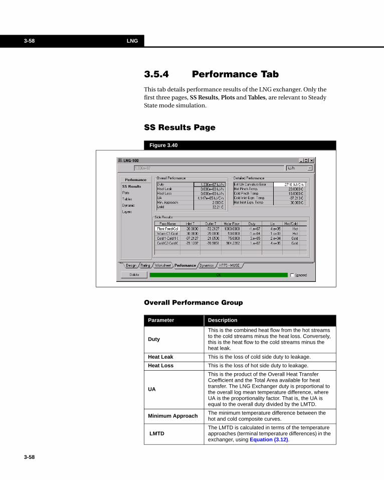
3-58 LNG
3-58
3.5.4 Performance TabThis tab details performance results of the LNG exchanger. Only the first three pages, SS Results, Plots and Tables, are relevant to Steady State mode simulation.
SS Results Page
Overall Performance Group
Figure 3.40
Parameter Description
Duty
This is the combined heat flow from the hot streams to the cold streams minus the heat loss. Conversely, this is the heat flow to the cold streams minus the heat leak.
Heat Leak This is the loss of cold side duty to leakage.
Heat Loss This is the loss of hot side duty to leakage.
UA
This is the product of the Overall Heat Transfer Coefficient and the Total Area available for heat transfer. The LNG Exchanger duty is proportional to the overall log mean temperature difference, where UA is the proportionality factor. That is, the UA is equal to the overall duty divided by the LMTD.
Minimum Approach The minimum temperature difference between the hot and cold composite curves.
LMTDThe LMTD is calculated in terms of the temperature approaches (terminal temperature differences) in the exchanger, using Equation (3.12).

Heat Transfer Equipment 3-59
where:
Detailed Performance Group
Side Results Group
The Side Results group displays information on each Pass. For each side, the Inlet and Outlet Temperatures, Molar Flow, Duty, UA and the Hot/Cold designation are displayed.
Plots Page
You can plot composite curves or individual pass curves for the LNG. Use the Plot check boxes to specify which curve(s) you want displayed.
(3.12)∆TLM
∆T1 ∆T2–
∆T1 ∆T2⁄( )ln----------------------------------=
∆T1 Thot out, Tcold in,–=
∆T2 Thot in, Tcold o, ut–=
Parameter Description
Estimated UA Curvature Error
The LMTD is ordinarily calculated using constant heat capacity. An LMTD can also be calculated using linear heat capacity. In either case, a different UA will be predicted. The UA Curvature Error reflects the difference between these UAs.
Hot Pinch Temperature
The hot stream temperature at the minimum approach between composite curves.
Cold Pinch Temperature
The cold stream temperature at the minimum approach between composite curves.
Cold Inlet Equilibrium Temperature
The Equilibrium Temperature for the cold streams. When streams are not equilibrated (see Parameters page), the Equilibrium temperature is the coldest temperature of all cold inlet streams.
Hot Inlet Equilibrium Temperature
The Equilibrium Temperature for the hot streams. When streams are not equilibrated (see Parameters Page), the Equilibrium temperature is the hottest temperature of all hot inlet streams.
You can modify the appearance of the plot via the Graph Control view. Refer to Chapter 6 - Output Control of the User’s Guide for more information.
3-59

3-60 LNG
3-60
The following variables may be used for either the x or y-axis: Temperature, UA, Delta T, Enthalpy, Pressure and Heat Flow. Select the combination from the Plot Type drop down list. To view the plot area only, select the View Plot button.
Tables Page
On the Table page, you can examine the interval Temperature, Pressure, Heat Flow, Enthalpy, UA, Vapour Fraction and Delta T for each side of the Exchanger in a tabular format. Choose the side, Cold Composite or Hot Composite, by making a selection from the drop down list above the table.
Dynamic and Layers Pages
The Dynamic and Layers pages of the Performance tab display results from Dynamic mode operation. For more information on these pages, see the Dynamic Modeling guide.
Figure 3.41
Heat Transfer Equipment 3-61
3.5.5 Dynamics TabIf you are working exclusively in Steady State mode, you are not required to change any information on the pages accessible through this tab. For more information on running the LNG unit operations in Dynamics mode, see the Dynamic Modeling guide for further details.
3.5.6 HTFS-MUSE TabThe HTFS-MUSE tab integrates the HTFS’ MUSE application into the HYSYS LNG unit operation.
MUSE can perform a range of calculations on plate-fin heat exchangers, either simple two-stream exchangers, or complex ones with multiple streams. The basic calculation options are:
These calculation types all relate to co- or counter-current exchangers.
This tab is made up of nine pages:
• Exchanger• Process
MUSE Calculation Modes
Simulation
This determines the heat load, pressure changes and outlet conditions for each stream in the exchanger, based on an exchanger you specify, and given stream inlet conditions.
Layer by Layer Simulation
As for normal simulation, but on a layer by layer rather than stream by stream basis. This option lets you assess the stacking pattern in which layers of the various streams are arranged.
Thermosyphon
This determines the performance of an exchanger, with a geometry you specify, with one stream operating as a thermosyphon. The exchanger can either be internal to the column or outside it and connected via pipe work. You can specify either the head of liquid driving the thermosyphon flow, or the thermosyphon stream flowrate, leaving the program to calculate the one you do not specify.
Design
This will produce a “first shot” design of a heat exchanger to meet a heat load duty and pressure drop limits, which you specify for each stream. This should be a useful indication of what a specialist manufacturer would provide. A final design of a plate-fin exchanger must, however, come from a manufacturer, who can use proprietary finning and specialist design and manufacturing techniques.
3-61
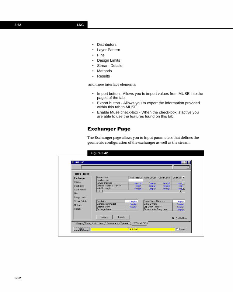
3-62 LNG
3-62
• Distributors• Layer Pattern• FIns• Design Limits• Stream Details• Methods• Results
and three interface elements:
• Import button - Allows you to import values from MUSE into the pages of the tab.
• Export button - Allows you to export the information provided within this tab to MUSE.
• Enable Muse check-box - When the check-box is active you are able to use the features found on this tab.
Exchanger Page
The Exchanger page allows you to input parameters that defines the geometric configuration of the exchanger as well as the stream.
Figure 3.42
Heat Transfer Equipment 3-63
The group box located on the top of the page is for specifying the stream geometry and consists of the following fields:
Field Description
Flow Direction
There are three options that you can choose from to define the Flow direction of this stream.
• flow away from end A, Up (B to A)• flow towards end A, Down (A to B)• No Flow
Normal design practice is for hot streams to flow from end A (which is at the top of the exchanger), while cold streams flow towards end A.
Number of Layers
Allows you to enter the total number of layers a stream occupies in the exchanger. If there is more than one exchanger in parallel, enter the number for one exchanger only.
This item may be omitted if a layer pattern is input. If you provide both, however, they are cross-checked, which can be useful in detecting errors in a layer pattern input. When they are inconsistent, a warning is produced.
If a stream is re-distributed, and occupies extra layers for part of its length, enter the basic number of layers only here, and specify the additional layers on the Distributors page.
Distance to Start of Main Fin
Allows you to enter the distance to the start of a stream's main finning from the fixed reference point. If omitted, the default is zero.
If this distance is less than the distance to the start of the effective length, then there is a region of main fin where pressure drop, but not heat transfer, is evaluated. If this distance is greater than that to the start of the effective length, then the stream will have a draw-on or draw-off point part way along the exchanger.
Main Fin Length
Allows you to enter the length of the main fin for the stream. If the stream uses more than one type of main fin, enter the length of the first fin, counting from the stream inlet.
3-63

3-64 LNG
3-64
The remainder of the group boxes located on this page are for specifying the exchangers geometry and consists of the following fields:
Field Description
Orientation
Plate FIn heat exchangers are normally vertical, with flow up or down. Enter 1.0 for vertical exchangers with the reference end, end A at the top/ For horizontal or inclined exchangers, see the MUSE help file.
Exchangers in Parallel
More than one exchanger in parallel may be used when stream flowrates, or thermal duties are too large to be handled by a single exchanger. In all cases the exchangers are assumed to be identical, and no calculations are performed on pressure losses in connecting pipe work.
Effective Width The effective flow width is the total width of the exchanger less the widths of the two side bars.
Exchanger Metal
Plate Fin exchangers for LNG and other cryogenic duties are made of aluminium. For other exchangers, you can select from:
• aluminium• stainless steel• titanium
Parting Sheet Thickness
The thickness of the separating plates (parting sheets) between layers is used to determine the exchanger stack height, and also has an effect on the metal resistance to heat transfer.
Side Bar Width
Side bars form the sides and ends of each layer. This item does not usually affect the calculated results, with the exception of longitudinal conduction calculations.
Cap Sheet Thickness
The stack height is the sum of the fin heights and parting sheet thicknesses for every layer in the exchanger, plus the thickness of the two side plates (cap sheets).
Fin Number for Empty Layer
If you specify a layer pattern with some layers containing no streams enter the fin number to identify the fins used in such layers.
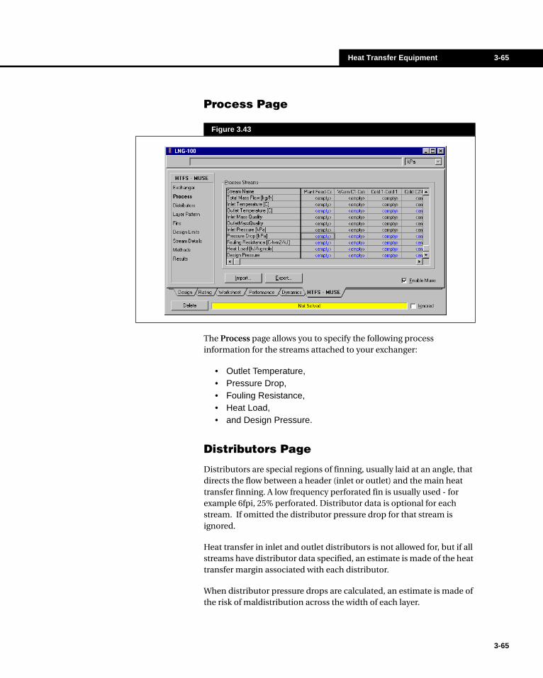
Heat Transfer Equipment 3-65
Process Page
The Process page allows you to specify the following process information for the streams attached to your exchanger:
• Outlet Temperature,• Pressure Drop,• Fouling Resistance,• Heat Load,• and Design Pressure.
Distributors Page
Distributors are special regions of finning, usually laid at an angle, that directs the flow between a header (inlet or outlet) and the main heat transfer finning. A low frequency perforated fin is usually used - for example 6fpi, 25% perforated. Distributor data is optional for each stream. If omitted the distributor pressure drop for that stream is ignored.
Heat transfer in inlet and outlet distributors is not allowed for, but if all streams have distributor data specified, an estimate is made of the heat transfer margin associated with each distributor.
When distributor pressure drops are calculated, an estimate is made of the risk of maldistribution across the width of each layer.
Figure 3.43
3-65
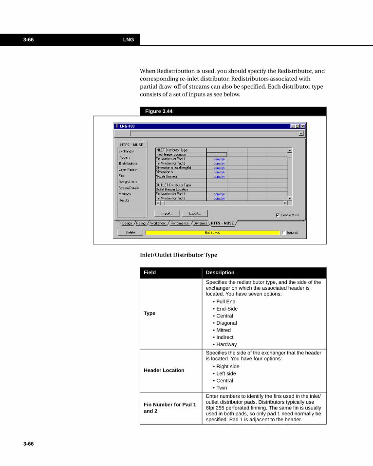
3-66 LNG
3-66
When Redistribution is used, you should specify the Redistributor, and corresponding re-inlet distributor. Redistributors associated with partial draw-off of streams can also be specified. Each distributor type consists of a set of inputs as see below.
Inlet/Outlet Distributor Type
Figure 3.44
Field Description
Type
Specifies the redistributor type, and the side of the exchanger on which the associated header is located. You have seven options:
• Full End• End-Side• Central• Diagonal• Mitred• Indirect• Hardway
Header Location
Specifies the side of the exchanger that the header is located. You have four options:
• Right side• Left side• Central• Twin
Fin Number for Pad 1 and 2
Enter numbers to identify the fins used in the inlet/outlet distributor pads. Distributors typically use 6fpi 255 perforated finning. The same fin is usually used in both pads, so only pad 1 need normally be specified. Pad 1 is adjacent to the header.

Heat Transfer Equipment 3-67
Redistributor Type
Dimension a (axial length)
Enter dimension a for the inlet/outlet distributor. Dimension a is the length along the exchanger occupied by the distributor.
Dimension b
Enter dimension b for the inlet/outlet distributor. This is the header diameter for End Side, Central, Indirect and Hardway distributors, and the Pad 1 length for Mitred distributors. It is not needed for Full End of Diagonal distributors.
Nozzle DIameterEnter the internal diameter of the inlet/outlet nozzle. If omitted the inlet/outlet nozzle pressure loss will not be calculated.
Field Description
Field Description
Type
Specifies the redistributor type, and the side of the exchanger on which the associated header is located. You have four options:
• Standard• Twin• Hardway• Hardway Twin
Header Location
Specifies the side of the exchanger that the header is located. You have three options:
• Right side• Left side• Twin
Distance to Redistributor
Specifies the distance to the redistributor from the inlet.
Fin Number for Pad 1, 2 and 3
Enter numbers to identify the fins used in the redistributor. The same fin is usually used in all pads, so only pad 1 need normally be specified. In a dividing redistributor, flow that remains in the layers flows through Pad 1 then Pad 2, while Pad 3 carries the flow that goes to other layers.
Dimension a (axial length)
Enter dimension a, the length along the exchanger occupied by the redistributor.
Dimension b
Enter dimension b for the redistributor. In a conventional dividing redistributor, this is the entry width associated with the flow that remains in the same layer.
3-67

3-68 LNG
3-68
Re-Inlet Distributor Type
Layer Pattern Page
The Layer Pattern page allows you to define the sequence of stream numbers that comprise the exchanger. The layer pattern itself gives the sequence of layers, while the Layer Definition table lets you define the sequence of streams in each layer. The layer pattern is mandatory input for Layer-by-Layer simulations, but optional for stream by stream. If no layer pattern is provided, the number of layers for each stream must be input.
Field Description
Type
Specifies the re-inlet distributor type. This can be any form of side entry/exit distributor. You have five options:
• None• Diagonal• Mitred• Indirect• Hardway
Fin Number for Pad 1 and 2
Enter numbers to identify the fins used in the re-inlet distributor pads. The same fin is usually used in both pads, so only pad 1 need normally be specified. Pad 1 is adjacent to the header.
Dimension a (axial length)
Enter dimension a, the length along the exchanger occupied by the re-inlet distributor.
Dimension b Enter dimension b for the re-inlet distributor.
Extra Layers/Draw Off Fraction
For a re-inlet distributor that directs flow to a number of extra layers, enter the number of extra layers.
For a re-inlet distributor that collects from the extra layers, to direct it back to the basic number of layers, enter the number of extra layers with a minus sign.
If there are no extra layers, but the stream is partially drawn off, enter the fraction of the stream which is drawn off.

Heat Transfer Equipment 3-69
Layer Pattern
Enter the sequence of layers forming the layer pattern (stacking pattern). The pattern can be identified as a sequence of layer identifiers, each identified by a letter, such as ABABABCAB. Though in simple cases, for example when there is only one stream per layer, the layer pattern can be specified as sequence of streams, for example 121213412.
Repeated sequences can be written in brackets, for example (121213/5)1312 means that the sequence 121213 occurs five times, followed by 1312. Spaces in the pattern are ignored and brackets cannot be embedded in brackets. A stream number’s sequence may contain zeros to indicate completely empty layers.
A layer pattern may terminate in M or MM to indicate that the pattern has central symmetry. MM indicates that the central layer is repeated, M that the symmetry is about the centre of the final layer. When The pattern is defined in terms of letters, use | or ||, not M's, to indicate mirror symmetry.
Figure 3.45
3-69

3-70 LNG
3-70
Layer Definition
For each (alphabetic) layer identifier in the pattern specify the stream or sequence of streams along the exchanger from end A, within each layer type. This is only needed when a pattern is defined in terms of layer types (A,B,C etc.) rather than streams, 1, 2, 4 etc.
The Layer Definition facility is only available in MUSE 3.20 and later versions.
Fins Page
The Fins page allows you to specify data on fin geometry. When a fin is specified, the corresponding fin performance data from the fin manufacturer (friction factors and Colburn j factors over a range of Reynolds numbers) should be input when available. If they are not available, they will be estimated using generalized HTFS correlations for particular fin types.
Fin numbers are used to identify the particular fin used as main fin or distributor fin for each stream. Fin numbers up to 20 identify fins that data is supplied in the program input.
The Fin Geometry groups consists of two buttons and a table. The two buttons allows you to add and remove fins from the heat exchanger, while the table allows you to specify each fin’s geometry. The table is made up of the following fields.
Figure 3.46

Heat Transfer Equipment 3-71
As mentioned above the corresponding fin performance data from the fin manufacturer, if available, should be input into the Fin Performance group. To specify the data, select the fin number from the list of fins and enter the data in the appropriate fields. The Plot Performance button displays a plot of the performance data for all of the fins.
Field Description
Fin Type
There are four main types of fin
• Plain• Perforated• Serrated, or offset-strip• Wavy or herringbone
For details of when each type should be used refer to the MUSE Help.
Prandtl No. Correlation to Cj
This parameter is important for high viscosity fluids in plain or perforated fins.
The Colburn j factors assumes that Cj is a function of Re only, but this is not true at low Reynolds numbers (below 1000), where there is also Prandtl number dependence.
If you supply Re-f-Cj data at a Pr appropriate to the fluids used, omit this item. If you specify Pr=1 data, specify 1 for a full correction, or a value between 0 and 1 for a partial correction. See the MUSE Help for more details.
Fin Height
The fin height is the distance between the separating plates (parting sheets). This applies to all fin types.
All the fins (main fin and distributor) for a stream must have the same height. A warning is issued if this is not so.
Fin Thickness Enter the fin thickness.
FIn Frequency
Enter the number of fins per unit of length. This item may be zero if no fins are present.
Common fin frequencies are 16, 18 or 21 ft/in for main fins, and 6 or 8 ft/in for distributor fins.
Fin Porosity For perforated fins, enter the fin porosity as a fraction of the metal lost as holes.
Fin Serration Length
For serrated fins enter the fin serration length. The default is 3 mm (approximately 1/8 inch), which is typical of values used by most manufacturers.
This input item is only needed for long-serration length serrated fins.
3-71
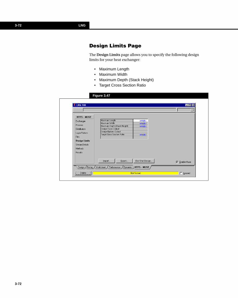
3-72 LNG
3-72
Design Limits Page
The Design Limits page allows you to specify the following design limits for your heat exchanger:
• Maximum Length• Maximum Width• Maximum Depth (Stack Height)• Target Cross Section Ratio
Figure 3.47
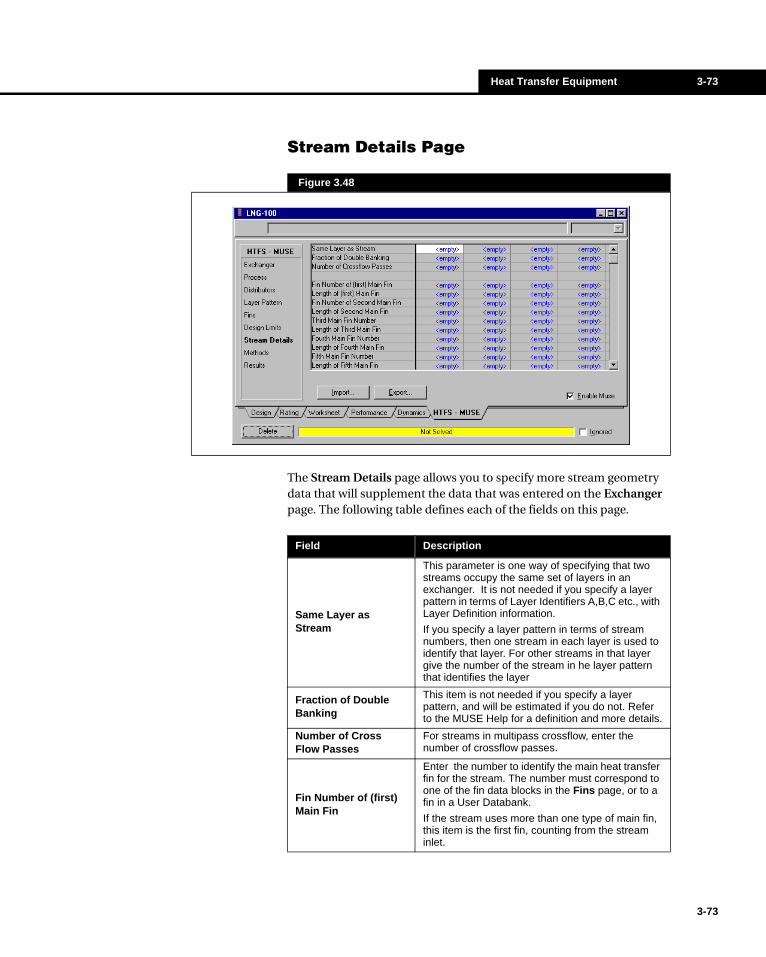
Heat Transfer Equipment 3-73
Stream Details Page
The Stream Details page allows you to specify more stream geometry data that will supplement the data that was entered on the Exchanger page. The following table defines each of the fields on this page.
Figure 3.48
Field Description
Same Layer as Stream
This parameter is one way of specifying that two streams occupy the same set of layers in an exchanger. It is not needed if you specify a layer pattern in terms of Layer Identifiers A,B,C etc., with Layer Definition information.
If you specify a layer pattern in terms of stream numbers, then one stream in each layer is used to identify that layer. For other streams in that layer give the number of the stream in he layer pattern that identifies the layer
Fraction of Double Banking
This item is not needed if you specify a layer pattern, and will be estimated if you do not. Refer to the MUSE Help for a definition and more details.
Number of Cross Flow Passes
For streams in multipass crossflow, enter the number of crossflow passes.
Fin Number of (first) Main Fin
Enter the number to identify the main heat transfer fin for the stream. The number must correspond to one of the fin data blocks in the Fins page, or to a fin in a User Databank.
If the stream uses more than one type of main fin, this item is the first fin, counting from the stream inlet.
3-73
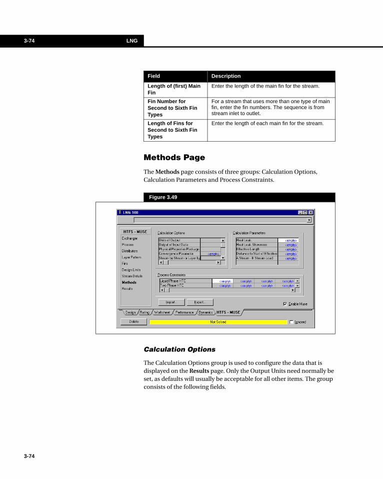
3-74 LNG
3-74
Methods Page
The Methods page consists of three groups: Calculation Options, Calculation Parameters and Process Constraints.
Calculation Options
The Calculation Options group is used to configure the data that is displayed on the Results page. Only the Output Units need normally be set, as defaults will usually be acceptable for all other items. The group consists of the following fields.
Length of (first) Main Fin
Enter the length of the main fin for the stream.
Fin Number for Second to Sixth Fin Types
For a stream that uses more than one type of main fin, enter the fin numbers. The sequence is from stream inlet to outlet.
Length of Fins for Second to Sixth Fin Types
Enter the length of each main fin for the stream.
Field Description
Figure 3.49
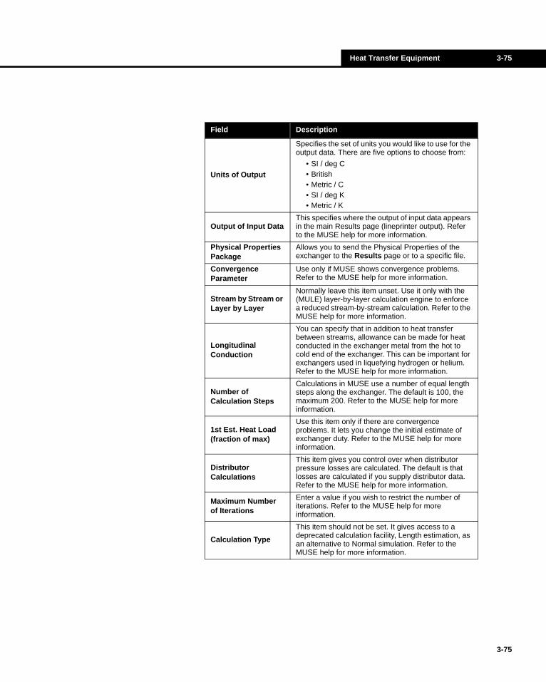
Heat Transfer Equipment 3-75
Field Description
Units of Output
Specifies the set of units you would like to use for the output data. There are five options to choose from:
• SI / deg C• British• Metric / C• SI / deg K• Metric / K
Output of Input DataThis specifies where the output of input data appears in the main Results page (lineprinter output). Refer to the MUSE help for more information.
Physical Properties Package
Allows you to send the Physical Properties of the exchanger to the Results page or to a specific file.
Convergence Parameter
Use only if MUSE shows convergence problems. Refer to the MUSE help for more information.
Stream by Stream or Layer by Layer
Normally leave this item unset. Use it only with the (MULE) layer-by-layer calculation engine to enforce a reduced stream-by-stream calculation. Refer to the MUSE help for more information.
Longitudinal Conduction
You can specify that in addition to heat transfer between streams, allowance can be made for heat conducted in the exchanger metal from the hot to cold end of the exchanger. This can be important for exchangers used in liquefying hydrogen or helium. Refer to the MUSE help for more information.
Number of Calculation Steps
Calculations in MUSE use a number of equal length steps along the exchanger. The default is 100, the maximum 200. Refer to the MUSE help for more information.
1st Est. Heat Load (fraction of max)
Use this item only if there are convergence problems. It lets you change the initial estimate of exchanger duty. Refer to the MUSE help for more information.
Distributor Calculations
This item gives you control over when distributor pressure losses are calculated. The default is that losses are calculated if you supply distributor data. Refer to the MUSE help for more information.
Maximum Number of Iterations
Enter a value if you wish to restrict the number of iterations. Refer to the MUSE help for more information.
Calculation Type
This item should not be set. It gives access to a deprecated calculation facility, Length estimation, as an alternative to Normal simulation. Refer to the MUSE help for more information.
3-75
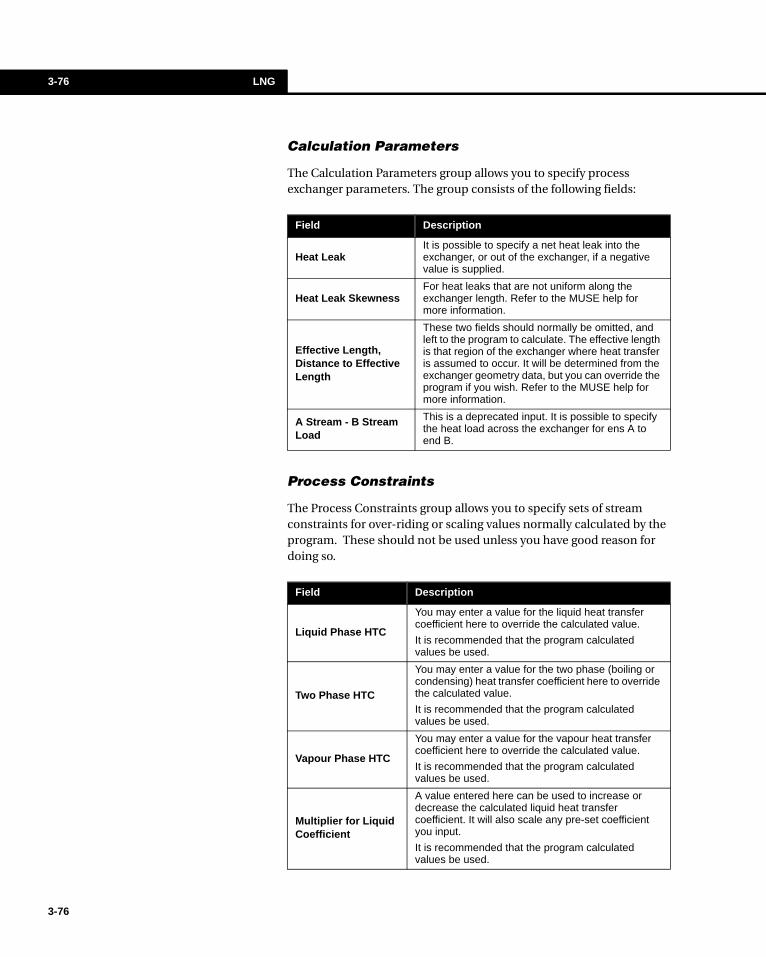
3-76 LNG
3-76
Calculation Parameters
The Calculation Parameters group allows you to specify process exchanger parameters. The group consists of the following fields:
Process Constraints
The Process Constraints group allows you to specify sets of stream constraints for over-riding or scaling values normally calculated by the program. These should not be used unless you have good reason for doing so.
Field Description
Heat LeakIt is possible to specify a net heat leak into the exchanger, or out of the exchanger, if a negative value is supplied.
Heat Leak SkewnessFor heat leaks that are not uniform along the exchanger length. Refer to the MUSE help for more information.
Effective Length, Distance to Effective Length
These two fields should normally be omitted, and left to the program to calculate. The effective length is that region of the exchanger where heat transfer is assumed to occur. It will be determined from the exchanger geometry data, but you can override the program if you wish. Refer to the MUSE help for more information.
A Stream - B Stream Load
This is a deprecated input. It is possible to specify the heat load across the exchanger for ens A to end B.
Field Description
Liquid Phase HTC
You may enter a value for the liquid heat transfer coefficient here to override the calculated value.
It is recommended that the program calculated values be used.
Two Phase HTC
You may enter a value for the two phase (boiling or condensing) heat transfer coefficient here to override the calculated value.
It is recommended that the program calculated values be used.
Vapour Phase HTC
You may enter a value for the vapour heat transfer coefficient here to override the calculated value.
It is recommended that the program calculated values be used.
Multiplier for Liquid Coefficient
A value entered here can be used to increase or decrease the calculated liquid heat transfer coefficient. It will also scale any pre-set coefficient you input.
It is recommended that the program calculated values be used.

Heat Transfer Equipment 3-77
Results Page
The exchanger results are displayed on this page. The results are created in a text format that can be exported to HTFS-MUSE.
Multiplier for Two Phase Coefficient
A value entered here can be used to increase or decrease the calculated boiling or condensing heat transfer coefficient. It will also scale any pre-set coefficient you input.
It is recommended that the program calculated values be used.
Multiplier for Vapour Coefficient
A value entered here can be used to increase or decrease the calculated vapour or gas heat transfer coefficient. It will also scale any pre-set coefficient you input.
It is recommended that the program calculated values be used.
Pressure Drop Multiplier
Enter the number that the calculated frictional pressure gradient (liquid, two phase or vapour) should be multiplied. It is not possible to scale the pressure drops of each phase separately.
It is recommended that the program calculated values be used.
Precalculated Arrays Flag
This input lets you override an internal calculation flag, it is best left unset. See the MUSE help for more details
Preset deltaT for Boiling
This input provides a variant on the boiling method, it is best left unset. See the MUSE help for more details
Field Description
3-77
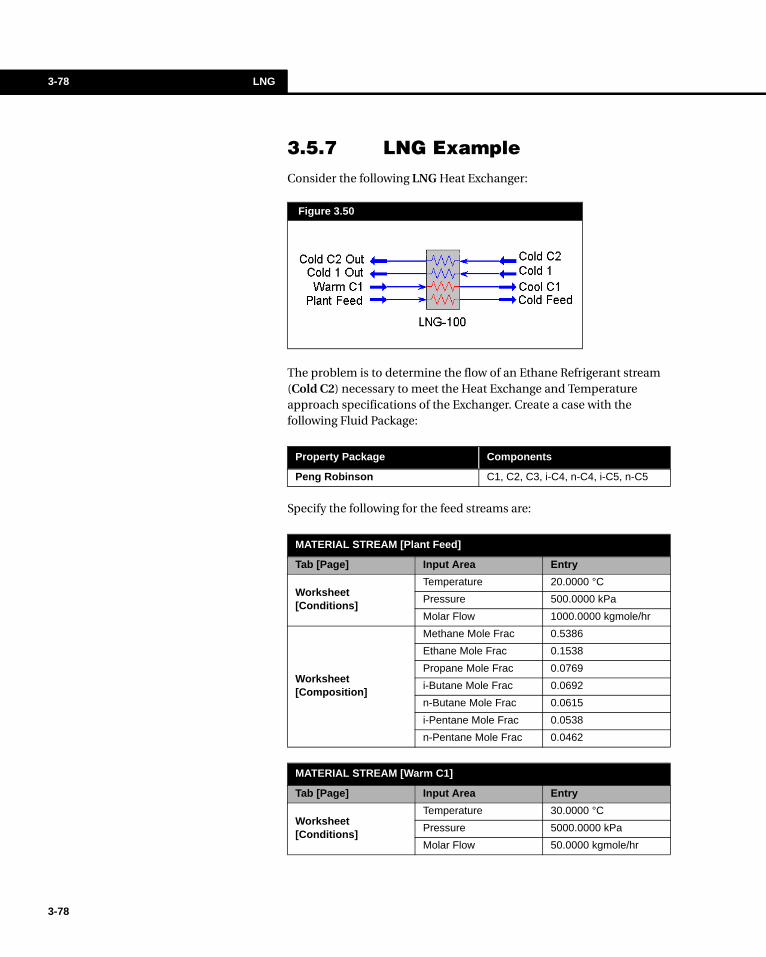
3-78 LNG
3-78
3.5.7 LNG ExampleConsider the following LNG Heat Exchanger:
The problem is to determine the flow of an Ethane Refrigerant stream (Cold C2) necessary to meet the Heat Exchange and Temperature approach specifications of the Exchanger. Create a case with the following Fluid Package:
Specify the following for the feed streams are:
Figure 3.50
Property Package Components
Peng Robinson C1, C2, C3, i-C4, n-C4, i-C5, n-C5
MATERIAL STREAM [Plant Feed]
Tab [Page] Input Area Entry
Worksheet [Conditions]
Temperature 20.0000 °C
Pressure 500.0000 kPa
Molar Flow 1000.0000 kgmole/hr
Worksheet [Composition]
Methane Mole Frac 0.5386
Ethane Mole Frac 0.1538
Propane Mole Frac 0.0769
i-Butane Mole Frac 0.0692
n-Butane Mole Frac 0.0615
i-Pentane Mole Frac 0.0538
n-Pentane Mole Frac 0.0462
MATERIAL STREAM [Warm C1]
Tab [Page] Input Area Entry
Worksheet [Conditions]
Temperature 30.0000 °C
Pressure 5000.0000 kPa
Molar Flow 50.0000 kgmole/hr
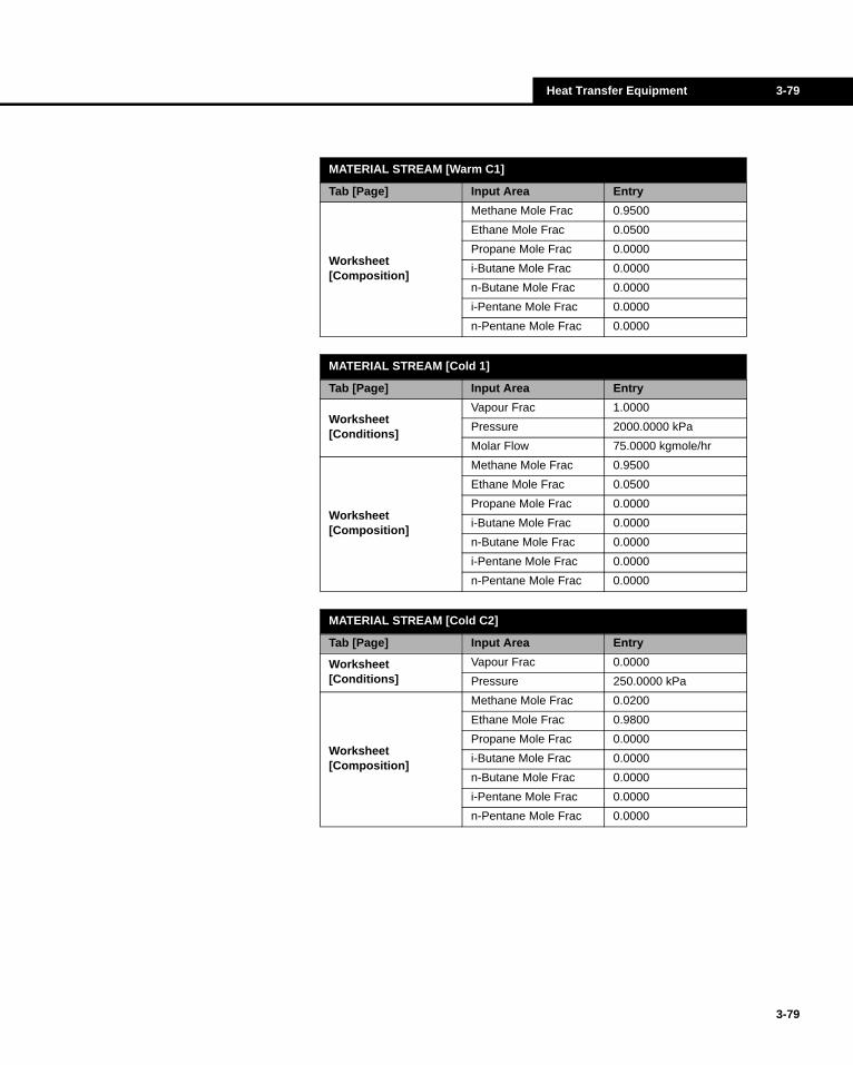
Heat Transfer Equipment 3-79
Worksheet [Composition]
Methane Mole Frac 0.9500
Ethane Mole Frac 0.0500
Propane Mole Frac 0.0000
i-Butane Mole Frac 0.0000
n-Butane Mole Frac 0.0000
i-Pentane Mole Frac 0.0000
n-Pentane Mole Frac 0.0000
MATERIAL STREAM [Cold 1]
Tab [Page] Input Area Entry
Worksheet [Conditions]
Vapour Frac 1.0000
Pressure 2000.0000 kPa
Molar Flow 75.0000 kgmole/hr
Worksheet [Composition]
Methane Mole Frac 0.9500
Ethane Mole Frac 0.0500
Propane Mole Frac 0.0000
i-Butane Mole Frac 0.0000
n-Butane Mole Frac 0.0000
i-Pentane Mole Frac 0.0000
n-Pentane Mole Frac 0.0000
MATERIAL STREAM [Cold C2]
Tab [Page] Input Area Entry
Worksheet [Conditions]
Vapour Frac 0.0000
Pressure 250.0000 kPa
Worksheet [Composition]
Methane Mole Frac 0.0200
Ethane Mole Frac 0.9800
Propane Mole Frac 0.0000
i-Butane Mole Frac 0.0000
n-Butane Mole Frac 0.0000
i-Pentane Mole Frac 0.0000
n-Pentane Mole Frac 0.0000
MATERIAL STREAM [Warm C1]
Tab [Page] Input Area Entry
3-79
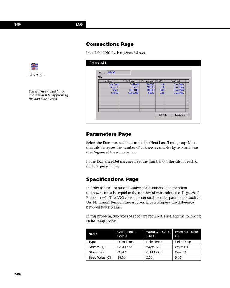
3-80 LNG
3-80
Connections Page
Install the LNG Exchanger as follows.
Parameters Page
Select the Extremes radio button in the Heat Loss/Leak group. Note that this increases the number of unknown variables by two, and thus the Degrees of Freedom by two.
In the Exchange Details group, set the number of intervals for each of the four passes to 20.
Specifications Page
In order for the operation to solve, the number of independent unknowns must be equal to the number of constraints (i.e. Degrees of Freedom = 0). The LNG considers constraints to be parameters such as UA, Minimum Temperature Approach, or a temperature difference between two streams.
In this problem, two types of specs are required. First, add the following Delta Temp specs:
Figure 3.51
LNG Button
You will have to add two additional sides by pressing the Add Side button.
NameCold Feed - Cold 1
Warm C1 - Cold 1 Out
Warm C1 - Cold C1
Type Delta Temp Delta Temp Delta Temp
Stream (+) Cold Feed Warm C1 Warm C1
Stream (-) Cold 1 Cold 1 Out Cool C1
Spec Value [C] 15.00 2.00 5.00

Heat Transfer Equipment 3-81
Then add two Duty Ratio Specs:
On the Worksheet page, specify the Vapour Fraction of Cold C2 Out to be 1.
At this point, the Degrees of Freedom will be zero and the LNG will begin to solve. The status message at the bottom of the LNG property view will read Temperature Cross. Move to the Plots page to see that the Composite curves clearly show a temperature cross at the hot side entrance (see Figure 3.52).
A different approach that can be used is to remove the Temperature difference between Cold 1 Out and Warm C1, and instead specify a Minimum Temperature Approach for the Exchanger at 2oC.
Name Heat Leak Fraction Heat Loss Fraction
Type Duty Ratio Duty Ratio
Pass Heat Leak Heat Loss
Pass (/) Overall Overall
Spec Value 0.00 0.00
Figure 3.52
3-81

3-82 LNG
3-82
Return to the Specs page and clear the Active check box for the Warm C1 - Cold 1 Out specification. Add the minimum approach specification, as described to the below.
Results
Move to the Conditions page of the Worksheet tab of the LNG:
On the SS Results page of the Performance tab, you will find the Performance and the Side Results:
Name Min. T Approach
Type Min. Approach
Pass Overall
Spec Value 2.00 C
When you add the Minimum Temperature Approach specification, the LNG Exchanger quickly solves.
Figure 3.53
Figure 3.54
Piping Equipment 4-1
4 Piping Equipment
4-1
4.1 Mixer .............................................................................................................. 3
4.1.1 Design Tab ............................................................................................... 44.1.2 Rating Tab................................................................................................ 54.1.3 Worksheet Tab ......................................................................................... 54.1.4 Dynamics Tab .......................................................................................... 64.1.5 Example ................................................................................................... 6
4.2 Pipe Segment................................................................................................ 7
4.2.1 Calculation Modes ................................................................................... 84.2.2 Design Tab ............................................................................................. 124.2.3 Rating Tab.............................................................................................. 184.2.4 Worksheet Tab ....................................................................................... 274.2.5 Performance Tab.................................................................................... 284.2.6 Dynamics Tab ........................................................................................ 304.2.7 Deposition Tab ....................................................................................... 304.2.8 Pipe Example......................................................................................... 404.2.9 Modifying the Fittings Database............................................................. 42
4.3 Tee ............................................................................................................... 44
4.3.1 Design Tab ............................................................................................. 454.3.2 Ratings Tab ............................................................................................ 474.3.3 Worksheet Tab ....................................................................................... 474.3.4 Dynamics Tab ........................................................................................ 47
4.4 Valve ............................................................................................................ 48
4.4.1 Design Tab ............................................................................................. 494.4.2 Ratings Tab ............................................................................................ 504.4.3 Worksheet Tab ....................................................................................... 504.4.4 Dynamics Tab ........................................................................................ 504.4.5 Valve Example ....................................................................................... 50
4-2
4-2
4.5 Relief Valve ................................................................................................. 52
4.5.1 Design Tab ............................................................................................. 524.5.2 Ratings Tab ............................................................................................ 544.5.3 Worksheet Tab ....................................................................................... 544.5.4 Dynamics Tab ........................................................................................ 544.5.5 Relief Valve Example ............................................................................. 54
4.6 References.................................................................................................. 56
Piping Equipment 4-3
4.1 MixerThe MIXER operation combines two or more inlet streams to produce a single outlet stream. A complete heat and material balance is performed with the MIXER. That is, the one unknown temperature among the inlet and outlet streams will always be calculated rigorously. If the properties of all the inlet streams to the MIXER are known (temperature, pressure and composition), the properties of the outlet stream will be calculated automatically since the composition, pressure and enthalpy will be known for that stream.
The mixture pressure and temperature are usually the unknowns to be determined. However, the MIXER will also calculate backwards and determine the missing temperature for one of the inlet streams if the outlet is completely defined. In this latter case, the pressure must be known for all streams.
The MIXER will flash the outlet stream using the combined enthalpy. Note that when the inlet streams are completely known, no additional information needs to be specified for the outlet stream. The problem is completely defined; no degrees of freedom remain.
To ignore the Mixer during calculations, activate the Ignored check box. HYSYS will disregard the operation until you clear the check box.
To install the MIXER operation, press F12 and choose Mixer or select the Mixer button in the Object Palette.
Mixer Button
The resultant temperature of the mixed streams may be quite different than those of the feed streams due to mixing effects.
4-3
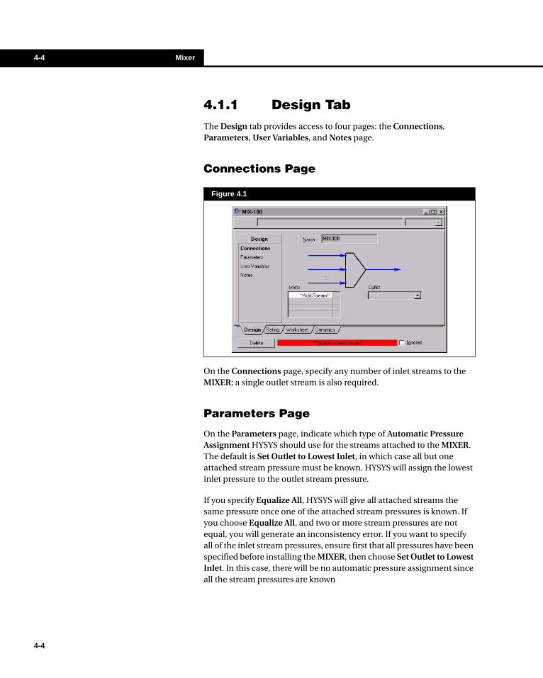
4-4 Mixer
4-4
4.1.1 Design TabThe Design tab provides access to four pages: the Connections, Parameters, User Variables, and Notes page.
Connections Page
On the Connections page, specify any number of inlet streams to the MIXER; a single outlet stream is also required.
Parameters Page
On the Parameters page, indicate which type of Automatic Pressure Assignment HYSYS should use for the streams attached to the MIXER. The default is Set Outlet to Lowest Inlet, in which case all but one attached stream pressure must be known. HYSYS will assign the lowest inlet pressure to the outlet stream pressure.
If you specify Equalize All, HYSYS will give all attached streams the same pressure once one of the attached stream pressures is known. If you choose Equalize All, and two or more stream pressures are not equal, you will generate an inconsistency error. If you want to specify all of the inlet stream pressures, ensure first that all pressures have been specified before installing the MIXER, then choose Set Outlet to Lowest Inlet. In this case, there will be no automatic pressure assignment since all the stream pressures are known
Figure 4.1

Piping Equipment 4-5
If you are uncertain of which pressure assignment to use, choose Set Outlet to Lowest Inlet. Only use Equalize All if you are completely sure that all the attached streams should have the same pressure. While the pressure assignment may seem to be extraneous, it is of special importance when the MIXER is being used to simulate the junction of multiple pipe nodes.
User Variables Page
The User Variables page allows you to create and implement variables in the HYSYS simulation case. For more information on implementing the User Variables option, see the User Variables chapter in the Customization Guide.
Notes Page
The Notes page provides an editor where you can record any remarks pertaining to the MIXER or to your simulation case in general.
4.1.2 Rating TabYou are not able to specify any rating information for the TEE operation in HYSYS.Process.
4.1.3 Worksheet TabThe Worksheet tab contains a summary of the information contained in the stream property view for all the streams attached to the unit operation. The Conditions, Properties, and Composition pages contain selected information from the corresponding pages of the Worksheet tab for the stream property view. The PF Specs page contains a summary of the stream property view Dynamics tab.
Note that if you select Equalize All and two or more of the attached streams have different pressures, a pressure inconsistency message will appear. In this case, you must either remove the pressure specifications for all but one of the attached streams, or select Set Outlet to Lowest Inlet. If you specify Set Outlet to Lowest Inlet, you can still set the pressures of all the streams.
4-5
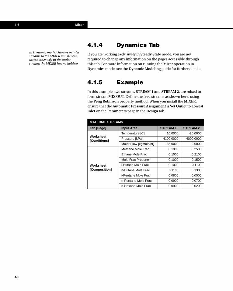
4-6 Mixer
4-6
4.1.4 Dynamics TabIf you are working exclusively in Steady State mode, you are not required to change any information on the pages accessible through this tab. For more information on running the Mixer operation in Dynamics mode, see the Dynamic Modeling guide for further details.
4.1.5 ExampleIn this example, two streams, STREAM 1 and STREAM 2, are mixed to form stream MIX OUT. Define the feed streams as shown here, using the Peng Robinson property method. When you install the MIXER, ensure that the Automatic Pressure Assignment is Set Outlet to Lowest Inlet on the Parameters page in the Design tab.
In Dynamic mode, changes in inlet streams to the MIXER will be seen instantaneously in the outlet stream; the MIXER has no holdup.
MATERIAL STREAMS
Tab [Page] Input Area STREAM 1 STREAM 2
Worksheet [Conditions]
Temperature [C] 10.0000 -20.0000
Pressure [kPa] 4100.0000 4000.0000
Molar Flow [kgmole/hr] 35.0000 2.0000
Worksheet [Composition]
Methane Mole Frac 0.1900 0.2500
Ethane Mole Frac 0.1500 0.2100
Mole Frac Propane 0.1000 0.1500
i-Butane Mole Frac 0.1000 0.1100
n-Butane Mole Frac 0.1100 0.1300
i-Pentane Mole Frac 0.0800 0.0500
n-Pentane Mole Frac 0.0900 0.0700
n-Hexane Mole Frac 0.0900 0.0200

Piping Equipment 4-7
The results can be viewed in the Worksheet tab as shown below.
4.2 Pipe SegmentThe PIPE SEGMENT is used to simulate a wide variety of piping situations ranging from single/multiphase plant piping with rigorous heat transfer estimation, to large capacity looped pipeline problems. It offers two pressure drop correlations: one developed by Gregory, Aziz and Mandhane, and the other by Beggs and Brill. A third option, OLGAS, is also available as a gradient method. Four levels of complexity in heat transfer estimation allow you to find a solution as rigorous as required while allowing for quick generalized solutions to well-known problems.
The PIPE SEGMENT offers three calculation modes: Pressure Drop, Flow, and Length; the appropriate mode will automatically be selected depending on the information supplied. In order to solve the pipe, you must supply enough information to completely define both the material balance and energy balance.
To ignore the PIPE SEGMENT during calculations, activate the Ignored check box. HYSYS will disregard the operation until you clear the check box.
To install the PIPE SEGMENT, press F12 and choose Pipe Segment from the Unit Ops view or select the Pipe Segment button in the Object Palette.
Figure 4.2
OLGAS is a third-party option which can be purchased through Hyprotech or SCANDPOWER.
Pipe Segment Button
4-7

4-8 Pipe Segment
4-8
Before the pages of the PIPE SEGMENT property view are described, the Calculation Modes and Material/Energy Balance calculations are explained.
4.2.1 Calculation ModesThere are three calculation modes: Pressure Drop, Length and Flow. The mode will automatically be assigned depending on what information is specified.
Regardless of which mode you use, you must specify the number of increments in the pipe. Calculations are performed in each increment; for instance, in the determination of the pressure drop, energy and mass balances are performed in each increment, and the outlet pressure in that increment is used as the inlet pressure to the next increment. This continues down the length of the pipe until the pipe outlet pressure is determined.
The Pipe can solve in either direction. The solution procedure generally starts at the end where the temperature is known (temperature is typically not known on both ends). HYSYS then begins stepping through the pipe from that point, using either the supplied pressure, or estimating a starting value. If the starting point is the pipe outlet, HYSYS steps backwards through the pipe. At the other end of the pipe, HYSYS compares the calculated solution to other known information and specifications, and if necessary, restarts the procedure with a new set of starting estimates.
Some specifics of each calculation mode are provided below:
Pressure Drop
Assuming that a feed, product and energy stream are attached to the pipe, the following information is required:
• Flow• Pipe length, diameter and elevation change• Heat transfer information• At least one stream temperature and one pressure
There are two different methods for calculating the pressure drop:
Method 1. If you specify the temperature and pressure at the same end of the pipe, then energy and mass balances are solved for each increment, and the temperature and pressure of the stream at the opposite end of the pipe are determined.
Note that HYSYS does not check for Sonic Flow during these calculations.
Delta P Method 1:
1. At the end where temperature and pressure are specified, solve for the outlet temperature and pressure in the first segment.
2. Move to the next segment, using the outlet conditions of the previous segment as the new inlet conditions.
3. Continue down the pipe until the outlet pressure and temperature are solved.

Piping Equipment 4-9
Method 2. If you supply temperature for one stream and pressure for the other, an iterative loop is required outside of the normal calculation procedure:
• First, a pressure is estimated for the stream which has the temperature specified.
• Second, the pressure and temperature for the stream at the opposite end of the pipe are determined from incremental energy and mass balances as in the first method.
• If the calculated pressure and user-specified pressure are not the same (within a certain tolerance), a new pressure is estimated and the incremental energy and mass balances are re-solved. This continues until the absolute difference of the calculated and user-specified pressures are less than a certain tolerance.
The calculated pressure drop accounts for fittings, frictional and hydrostatic effects.
Length
Assuming that the feed, product and energy stream are attached, the following information is required:
• Flow• Heat transfer information• Pipe diameter• Inlet and Outlet Pressure (or one stream Pressure and
Pressure Drop)• One stream temperature• Initial estimate of Length
For each segment, the Length estimate, along with the known stream specifications, are used to solve for the unknown stream temperature and pressure. If the calculated pressure is not equal to the actual pressure (within the user-specified tolerance), a new estimate will be made for the length, and calculations will continue.
A good initial guess and step size will greatly decrease the solving time.
Delta P Method 2:
1. Estimate a pressure for the stream which has a specified temperature .
2. At the end where the pressure is estimated, solve for the outlet temperature and pressure in the first segment.
3. Move to the next segment, using the outlet conditions of the previous segment as the new inlet conditions.
4. Continue down the pipe until the outlet pressure and temperature are solved.
5. If the calculated outlet pressure is not equal to the actual pressure, a new estimate is made for pressure (Return to 1).
Length Calculation:
1. Estimate a Length. At the end where temperature is specified, solve for the outlet temperature and pressure in the first segment.
2. Move to the next segment, using the outlet conditions of the previous segment as the new inlet conditions.
3. Continue down the pipe until the outlet pressure and temperature are solved.
4. If the calculated outlet pressure is not equal to the actual pressure, a new estimate is made for length. (Return to 1).
The Pipe will also solve for the length if you provide one pressure and two temperature specifications, and the duty.
4-9
4-10 Pipe Segment
4-10
Flow
Assuming that a feed, product and energy stream are attached to the pipe, the following information is required:
• Pipe Length and diameter• Heat transfer information• Inlet and Outlet Pressure (or one stream Pressure and
Pressure Drop)• One stream temperature• Initial estimate of Flow
Using the flow estimate and known stream conditions (at the end with the known temperature), HYSYS will calculate a pressure at the other end. If the calculated pressure is not equal to the actual pressure (within the user-specified tolerance), a new estimate will be made for the flow, and calculations will continue.
Again, a good initial guess will decrease the solving time significantly.
Incremental Material and Energy Balances
The overall algorithm consists of three nested loops. The outer loop iterates on the increments (Pressure, Length or Flow Mode), the middle loop solves for the temperature, and the inner loop solves for pressure. The middle and inner loops implement a secant method to speed convergence. The pressure and temperature are calculated as follows:
1. The inlet temperature and pressure are passed to the material/energy balance routine.
2. Using internal estimates for temperature and pressure gradients, the outlet temperature and pressure are calculated.
3. Average fluid properties are calculated based on the inlet and estimated outlet conditions.
4. These properties, along with the inlet pressure, are passed to the pressure gradient algorithm (Beggs and Brill, Gregory Aziz Mandhane, or OLGAS)
5. With the pressure gradient, the outlet pressure can be calculated.
6. The calculated pressure and estimate pressure are compared. If their difference exceeds a tolerance (0.01%), a new outlet pressure is estimated, and steps 3 to 6 are repeated.
7. Once the inner pressure loop has converged, the outlet temperature is calculated:
Flow Calculation:
1. Estimate Flow. At the end where temperature is specified, solve for the outlet temperature and pressure in the first segment.
2. Move to the next segment, using the outlet conditions of the previous segment as the inlet conditions.
3. Continue down the pipe until the outlet pressure and temperature are solved.
4. If the calculated outlet pressure is not equal to the actual pressure, a new estimate is made for the flow. (Return to 1).
Piping Equipment 4-11
• If U and the ambient temperature are specified, then the outlet temperature is determined from the following equations:
where: Q = Amount of heat transferred
U = Overall heat transfer coefficient
A = Outer heat transfer area
DTLM = Log mean temperature difference
Qin = Heat flow of inlet stream
Qout = Heat flow of outlet stream
• If both the inlet and outlet Pipe temperatures are known, the outlet temperature of the increment is calculated by linear interpolation. The attached duty stream then completes the energy balance.
• If duty is known, the outlet temperature is calculated from a Pressure-Enthalpy flash.
When the Increment outlet temperature is calculated, it is compared with the estimated outlet temperature. If their difference exceeds a tolerance (0.01oC), a new outlet temperature is estimated, and new fluid properties are calculated (return to step 3).
8. When both the temperature and pressure converge, the outlet results are passed to the inlet of the next increment, where calculations continue.
Q = UADTLM (4.1)
Q = Qin - Qout (4.2)
4-11

4-12 Pipe Segment
4-12
4.2.2 Design TabThe Design tab provides access to five pages: the Connections, Parameters, Calculation, User Variables, and Notes page.
Connections Page
On the Connections page, you must specify the Feed and Product material streams. This can be done by selecting existing streams from the drop down boxes list associated with the Feed and Product fields. You can also create new streams by selecting the particular field and enter the new stream name in the Edit Bar.
In addition to the material stream connections, you also have the option of attaching an Energy stream to the PIPE SEGMENT. You may also edit the operation name on this page.
Figure 4.3
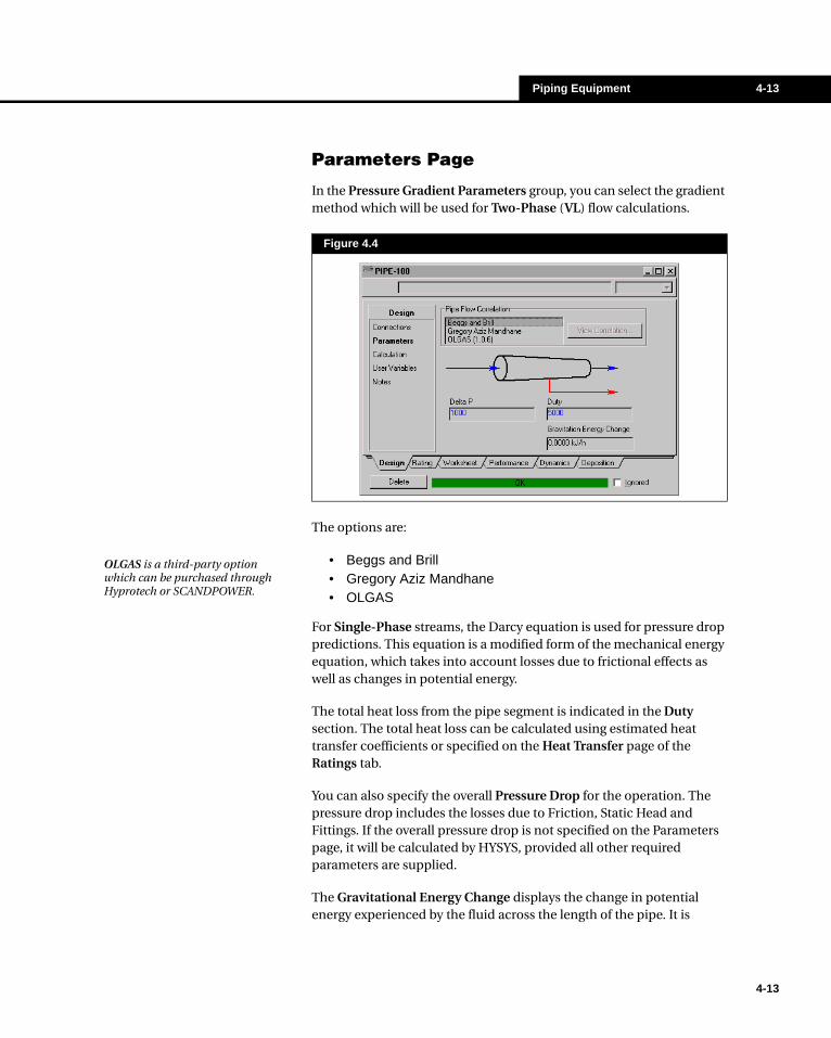
Piping Equipment 4-13
Parameters Page
In the Pressure Gradient Parameters group, you can select the gradient method which will be used for Two-Phase (VL) flow calculations.
The options are:
• Beggs and Brill• Gregory Aziz Mandhane• OLGAS
For Single-Phase streams, the Darcy equation is used for pressure drop predictions. This equation is a modified form of the mechanical energy equation, which takes into account losses due to frictional effects as well as changes in potential energy.
The total heat loss from the pipe segment is indicated in the Duty section. The total heat loss can be calculated using estimated heat transfer coefficients or specified on the Heat Transfer page of the Ratings tab.
You can also specify the overall Pressure Drop for the operation. The pressure drop includes the losses due to Friction, Static Head and Fittings. If the overall pressure drop is not specified on the Parameters page, it will be calculated by HYSYS, provided all other required parameters are supplied.
The Gravitational Energy Change displays the change in potential energy experienced by the fluid across the length of the pipe. It is
Figure 4.4
OLGAS is a third-party option which can be purchased through Hyprotech or SCANDPOWER.
4-13

4-14 Pipe Segment
4-14
determined for the overall elevation change, based on the sum of the elevation change specified for each segment on the Sizing page of the Rating tab.
When the pressure drop is specified, the PIPE SEGMENT can be used to calculate either the length of the PIPE SEGMENT or the flow of the material through the length of pipe.
Note that the calculation type (i.e. pressure drop, length, flow) is not explicitly specified. HYSYS determines what is to be calculated by the information that you provide.
Beggs and Brill Pressure Gradient
The Beggs and Brill6 method is based on work done with an air-water mixture at many different conditions, and is applicable for inclined flow. In the Beggs and Brill correlation, the flow regime is determined using the Froude number and inlet liquid content. The flow map used is based on horizontal flow and has four regimes: segregated, intermittent, distributed and transition. Once the flow regime has been determined, the liquid holdup for a horizontal pipe is calculated, using the correlation applicable to that regime. A factor is applied to this holdup to account for pipe inclination. From the holdup, a two-phase friction factor is calculated and the pressure gradient determined.
The overall pressure drop, which may be specified or calculated by HYSYS, is the sum of the Friction, Static Head, and Fittings pressure drops. When two liquid phases are present, appropriate volume based empirical mixing rules are implemented to calculate a single pseudo liquid phase. Therefore, caution should be exercised in interpreting the calculated pressure drops for three-phase systems. Actual pressure drops can vary dramatically for different flow regimes, and for emulsion systems.

Piping Equipment 4-15
Gregory Aziz Mandhane Pressure Gradient
For the Gregory Aziz Mandhane correlation, an appropriate model is used for predicting the overall pressure drop in two-phase flow.
Figure 4.5
Beggs and Brill Flow Regimes
0.010.0001 0.001 0.1 1 Input Liquid Content
Fro
ud
e N
um
ber
1
10
100
1000
Distributed
Segregated
Transition
Figure 4.6
Gregory Aziz Mandhane Flow Regimes
Superficial Gas Velocity (m/sec)
Su
per
fici
al L
iqu
id V
elo
city
(m
/sec
) Bubble, Elongated Bubble Flow
Stratified Flow
Dispersed Flow
Slug Flow
Wave Flow
Annular, Annular Mist Flow
4-15

4-16 Pipe Segment
4-16
OLGAS Pressure Gradient
OLGAS employs mechanistic models for each of the four major flow regimes: stratified, annular, slug and dispersed bubble flow. It is based in large part on data from the SINTEF two-phase flow laboratory in Norway.
It predicts the pressure gradient, liquid holdup and flow regime. It has been tested in one degree increments for all angles from horizontal to vertical. OLGAS gives one of the best overall predictions of pressure drop and liquid holdup of any currently available method. Contact your Hyprotech agent for more information on OLGAS.
Regime Model
Slugflow Mandhane, et. al. modification #1 of Lockhart-Martinelli
Dispersed Bubble Mandhane, et. al. modification #2 of Lockhart-Martinelli
Annular Mist Lockhart-Martinelli
Elongated Bubble
Mandhane, et. al. modification #1 of Lockhart-Martinelli
Stratified Lockhart-Martinelli
Wave Lockhart-Martinelli
All methods account for static head losses, while only the Beggs and Brill and OLGAS methods account for hydrostatic recovery. Beggs and Brill calculate the hydrostatic recovery as a function of the flow parameters and pipe angle.
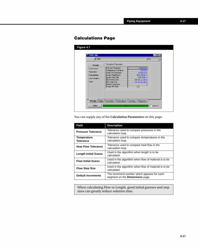
Piping Equipment 4-17
Calculations Page
You can supply any of the Calculation Parameters on this page:
Figure 4.7
Field Description
Pressure Tolerance Tolerance used to compare pressures in the calculation loop.
Temperature Tolerance
Tolerance used to compare temperatures in the calculation loop.
Heat Flow Tolerance Tolerance used to compare heat flow in the calculation loop.
Length Initial Guess Used in the algorithm when length is to be calculated.
Flow Initial Guess Used in the algorithm when flow of material is to be calculated.
Flow Step Size Used in the algorithm when flow of material is to be calculated
Default Increments The increment number which appears for each segment on the Dimensions page
When calculating Flow or Length, good initial guesses and step sizes can greatly reduce solution time.
4-17
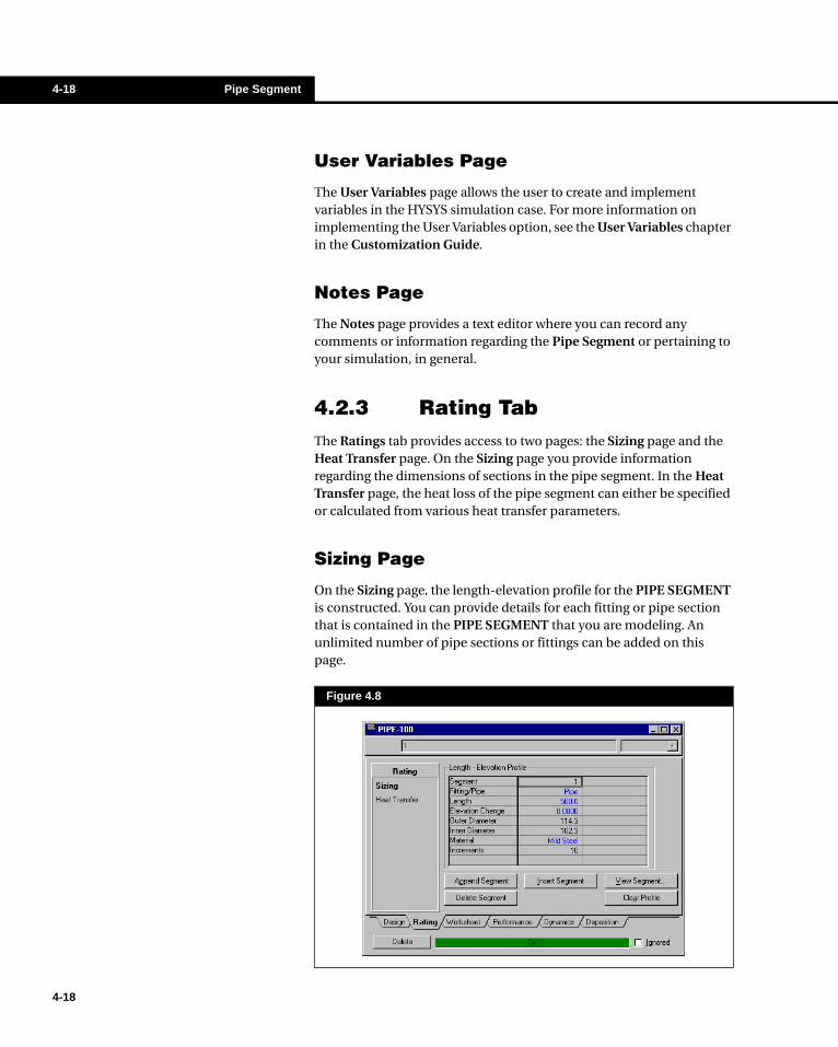
4-18 Pipe Segment
4-18
User Variables Page
The User Variables page allows the user to create and implement variables in the HYSYS simulation case. For more information on implementing the User Variables option, see the User Variables chapter in the Customization Guide.
Notes Page
The Notes page provides a text editor where you can record any comments or information regarding the Pipe Segment or pertaining to your simulation, in general.
4.2.3 Rating TabThe Ratings tab provides access to two pages: the Sizing page and the Heat Transfer page. On the Sizing page you provide information regarding the dimensions of sections in the pipe segment. In the Heat Transfer page, the heat loss of the pipe segment can either be specified or calculated from various heat transfer parameters.
Sizing Page
On the Sizing page, the length-elevation profile for the PIPE SEGMENT is constructed. You can provide details for each fitting or pipe section that is contained in the PIPE SEGMENT that you are modeling. An unlimited number of pipe sections or fittings can be added on this page.
Figure 4.8

Piping Equipment 4-19
For a given length of pipe which is modelled in HYSYS, the parameters of each segment is entered separately, as they are for each fitting.
The procedure for modeling a length of pipe is illustrated using the diagram shown below. In the diagram, the pipe length AD is represented by segments A, B, C, D and three fittings.
The table shown below displays the Fitting/Pipe, Length, and Elevation input that you require to represent the pipe length AD. Each pipe section and fitting is labelled as a segment. Note that horizontal pipe sections have an Elevation of 0. A positive elevation indicates that the outlet is higher than the inlet.
To fully define the pipe section segments, you must also specify pipe schedule, diameters (nominal or inner and outer), a material and a number of increments. The fittings require an inner diameter value.
Note, when you have only one pipe segment HYSYS will calculate the inner diameter of the pipe when a pressure difference and pipe length is specified.
Figure 4.9
X1
X2 X3Y1
Y2
F2
A
C
D
BExample of Pipe Sections and Fittings Modelled in the Pipe Segment Operation
Fittings
F3
F1
Number 1 2 3 4 5 6 7
Represented by A F1 B F2 C F3 D
Fitting/Pipe Pipe Fitting Pipe Fitting Pipe Fitting Pipe
Length x1 N/A y1 N/A x2 N/A
Elevation 0 N/A y1 N/A 0 N/A y2
x32 y2
2+
4-19

4-20 Pipe Segment
4-20
Adding Segments
You can add segments to the length-elevation profile by pressing the Add Segment button.
For each segment that you add, you must supply the following:
Figure 4.10
Field Description
Fitting/Pipe
Select a pipe section or one of the available fittings from the Edit Bar drop down list. If the list does not contain the fitting required, you can modify the fittings and change its K-factor for these calculations.
The fittings pressure drop is calculated as:
(4.3)
where: ρ = density
K =Pipe Fitting factor (K-factor)
V = Average superficial fluid velocity
gc = Gravitational constant
You may modify the Fittings Database, which is contained in file FITTING.DB. For more information, see Section 4.2.9 - Modifying the Fittings Database.
Length The actual length of the pipe segment. Not required for fittings.
Elevation Change
The change in vertical distance between the outlet and inlet of the pipe section. Positive values indicate that the outlet is higher than the inlet. Not required for fittings.
∆PρKV2
2gc--------------=

Piping Equipment 4-21
Viewing Segments
Once you have selected the segment type (pipe or fitting), you can supply detailed information concerning the highlighted segment. With the cursor located on a segment, press the View Segment button.
The Pipe Info dialog will appear for pipe sections. On this view, the following information is shown:.
Outer Diameter Outside diameter of the pipe or fitting.
Inner Diameter Inside diameter of the pipe or fitting.
MaterialSelect one of the available default materials or choose User Specified for the pipe section. Not required for fittings.
Increments The number of increments in which the pipe section is divided for calculation purposes.
Figure 4.11
Field Description
Pipe Schedule
Select one of the following:
• Actual - The nominal diameter cannot be specified. The inner diameter can be specified.
• Schedule 40• Schedule 80• Schedule 160
HYSYS contains a pipe database for three pipe schedules (40, 80, 160). If a schedule is specified, a popup menu will be displayed indicating the possible nominal pipe diameters that may be specified.
Nominal Diameter Provides the nominal diameter for the pipe section.
Field Description
Pipe fittings increase the pressure drop in the PIPE SEGMENT. The pressure drop is proportional to the K-factor for that fitting.
4-21

4-22 Pipe Segment
4-22
Removing a Segment
To remove a segment from the Length-Elevation Profile group box, highlight one of its parameters and press the Delete Segment button.
You can remove all input from the Length-Elevation Profile group box by pressing the Clear Profile button.
Inner DiameterFor Schedule 40, 80, or 160, this will be referenced from the database. For Actual Pipe Schedule, this can be specified directly by the user.
Pipe Material
Select a pipe material or choose User Specified. The pipe material type may be selected from the drop down list in the Edit Bar.The roughness factor is automatically supplied for pipe material chosen from this list. You may also specify the roughness factor manually. A table of pipe materials and corresponding Absolute Roughness factors is shown below.
Roughness A default value is provided based on the Pipe Material. You can specify a value if you wish.
Pipe Material Type Absolute Roughness, m
Drawn Tube 0.0000015
Mild Steel 0.0000457
Asphalted Iron 0.0001220
Galvanized Iron 0.0001520
Cast Iron 0.0002590
Smooth Concrete 0.0003050
Rough Concrete 0.0030500
Smooth Steel 0.0009140
Rough Steel 0.0091400
Smooth Wood Stave 0.0001830
Rough Wood Stave 0.0009140
Field Description
No confirmation is given by HYSYS before segments are removed.

Piping Equipment 4-23
Heat Transfer Page
On the Heat Transfer page, you can select the method that HYSYS will use for the heat transfer calculations. In the Specify By group box, select one of the radio buttons:
• By Segment - you specify the Ambient Temperature and HTC (Heat Transfer Coefficient) for each segment that was created on the Sizing page.
• Overall - one of four heat transfer methods will be applied to the whole pipe segment based on your input in the Heat Transfer Summary and Heat Transfer Coefficient Estimation group boxes. The heat transfer methods are:
Figure 4.12
Method Description
Duty Method
If the Overall heat duty of the segment is known, the energy balance can be calculated immediately. Each increment is assumed to have the same heat loss. This assumption is valid when the temperature profile is flat, indicating low heat transfer rates compared to the heat flows of the streams. This is the fastest solution method.
Stream Temperatures
If both inlet and outlet temperatures are specified, a linear profile is assumed and overall heat duty will be calculated. This method allows fast calculation when stream conditions are known.
4-23
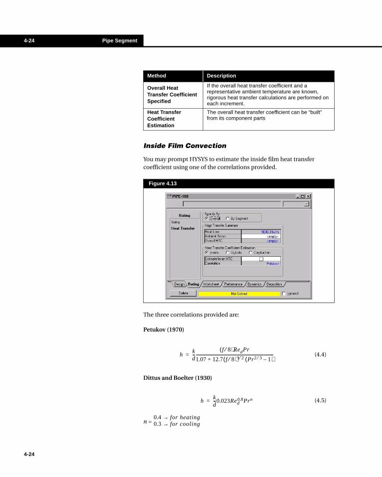
4-24 Pipe Segment
4-24
Inside Film Convection
You may prompt HYSYS to estimate the inside film heat transfer coefficient using one of the correlations provided.
The three correlations provided are:
Petukov (1970)
Dittus and Boelter (1930)
n =
Overall Heat Transfer Coefficient Specified
If the overall heat transfer coefficient and a representative ambient temperature are known, rigorous heat transfer calculations are performed on each increment.
Heat Transfer Coefficient Estimation
The overall heat transfer coefficient can be “built” from its component parts
Figure 4.13
Method Description
(4.4)hkd---
f 8⁄( )RedPr
1.07 12.7 f 8⁄( )1 2⁄ Pr2 3⁄ 1–( )+------------------------------------------------------------------------------=
(4.5)hkd---0.023Red
0.8Prn=
0.4 for heating→0.3 for cooling→
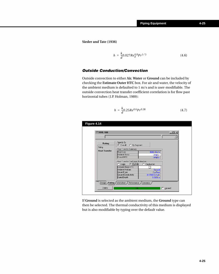
Piping Equipment 4-25
Sieder and Tate (1936)
Outside Conduction/Convection
Outside convection to either Air, Water or Ground can be included by checking the Estimate Outer HTC box. For air and water, the velocity of the ambient medium is defaulted to 1 m/s and is user-modifiable. The outside convection heat transfer coefficient correlation is for flow past horizontal tubes (J.P. Holman, 1989):
If Ground is selected as the ambient medium, the Ground type can then be selected. The thermal conductivity of this medium is displayed but is also modifiable by typing over the default value.
(4.6)hkd---0.027Red
0.8Pr1 3⁄=
(4.7)hkd---0.25Re0.6Pr0.38=
Figure 4.14
4-25
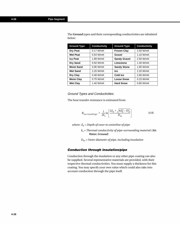
4-26 Pipe Segment
4-26
The Ground types and their corresponding conductivities are tabulated below:
Ground Types and Conductivities
The heat transfer resistance is estimated from:
where: Zb = Depth of cover to centreline of pipe
ks = Thermal conductivity of pipe-surrounding material (Air, Water, Ground)
Dot = Outer diameter of pipe, including insulation
Conduction through insulation/pipe
Conduction through the insulation or any other pipe coating can also be supplied. Several representative materials are provided, with their respective thermal conductivities. You must supply a thickness for this coating. You may specify your own value which could also take into account conduction through the pipe itself.
Ground Type Conductivity Ground Type Conductivity
Dry Peat 0.17 W/mK Frozen Clay 2.50 W/mK
Wet Peat 0.54 W/mK Gravel 1.10 W/mK
Icy Peat 1.89 W/mK Sandy Gravel 2.50 W/mK
Dry Sand 0.50 W/mK Limestone 1.30 W/mK
Moist Sand 0.95 W/mK Sandy Stone 1.95 W/mK
Wet Sand 2.20 W/mK Ice 2.20 W/mK
Dry Clay 0.48 W/mK Cold Ice 2.66 W/mK
Moist Clay 0.75 W/mK Loose Snow 0.15 W/mK
Wet Clay 1.40 W/mK Hard Snow 0.80 W/mK
(4.8)Rsurroundings1
2ks--------
2Zb 4Zb2 Dot
2–+
Dot--------------------------------------------ln=
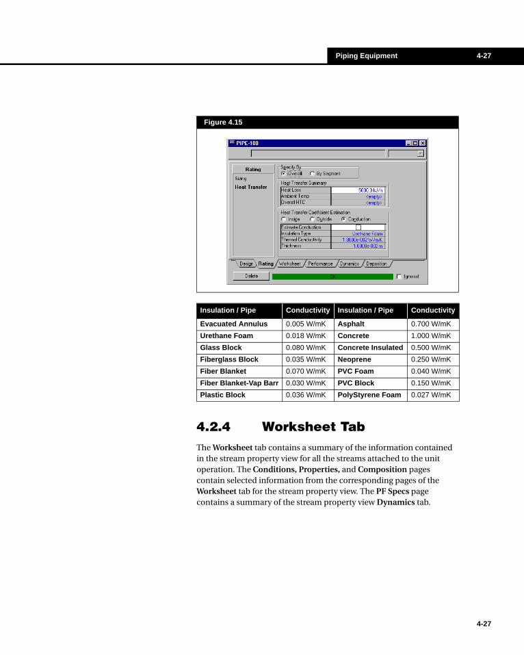
Piping Equipment 4-27
4.2.4 Worksheet TabThe Worksheet tab contains a summary of the information contained in the stream property view for all the streams attached to the unit operation. The Conditions, Properties, and Composition pages contain selected information from the corresponding pages of the Worksheet tab for the stream property view. The PF Specs page contains a summary of the stream property view Dynamics tab.
Figure 4.15
Insulation / Pipe Conductivity Insulation / Pipe Conductivity
Evacuated Annulus 0.005 W/mK Asphalt 0.700 W/mK
Urethane Foam 0.018 W/mK Concrete 1.000 W/mK
Glass Block 0.080 W/mK Concrete Insulated 0.500 W/mK
Fiberglass Block 0.035 W/mK Neoprene 0.250 W/mK
Fiber Blanket 0.070 W/mK PVC Foam 0.040 W/mK
Fiber Blanket-Vap Barr 0.030 W/mK PVC Block 0.150 W/mK
Plastic Block 0.036 W/mK PolyStyrene Foam 0.027 W/mK
4-27

4-28 Pipe Segment
4-28
4.2.5 Performance TabThe Performance tab provides access to the Profiles page. The Profiles page allows the user to access information about the fluid stream conditions for each specified increment in the pipe segment.
Profiles Page
The Profile page provides a summary table for the segments which make up the PIPE SEGMENT. The Distance (Length), Elevation and number of Increments are displayed for each segment. None of the values can be modified on this view.
By pressing the View Profile button, you access the Pipe Profile view, which consists of a Table page and a Plot page. The Table page displays the following information for each increment along the pipe segment:
• Length• Elevation• Pressure• Temperature• Heat Transferred• Flow Regime• Liquid Holdup• Friction Gradient• Static Gradient
Figure 4.16
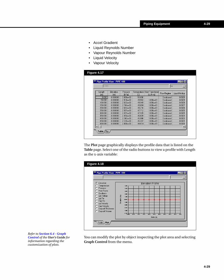
Piping Equipment 4-29
• Accel Gradient• Liquid Reynolds Number• Vapour Reynolds Number• Liquid Velocity• Vapour Velocity
The Plot page graphically displays the profile data that is listed on the Table page. Select one of the radio buttons to view a profile with Length as the x-axis variable:
You can modify the plot by object inspecting the plot area and selecting Graph Control from the menu.
Figure 4.17
Figure 4.18
Refer to Section 6.4 - Graph Control of the User’s Guide for information regarding the customization of plots.
4-29

4-30 Pipe Segment
4-30
4.2.6 Dynamics TabThis unit operation is currently not available for dynamic simulation.
4.2.7 Deposition TabThe deposition of the wax from the bulk oil onto the pipe wall is assumed to only be due to mass transfer, shear dispersion is not considered to be a significant factor. The rate of deposition is described by:
where: m’ = Deposition rate (kg/s)
k = Mass transfer coefficient (mole/m 2 s mole Fraction)
C = Local concentration of wax forming components (mole fraction)
Mwwax = Molecular weight of wax (kg/mole)
A = Cross-sectional area (m 2 )
The mass transfer coefficient is calculated using the following correlation:
where: Sc =
Re =
Sh =
D = Diffusivity of wax in oil (m 2 /s)
µ = Liquid viscosity (kg/ms)
ρl = Liquid density (kg/m 2 )
k = Mass transfer coefficient (mole/m 2 s mole fraction)
(4.9)m’ k Cwall Cbulk–( )AMwwax=
(4.10)Sh 0.015 Re
0.88× Sc
13---
=
µl
ρlD---------
VlρlDH
µl------------------
kDH
cD----------
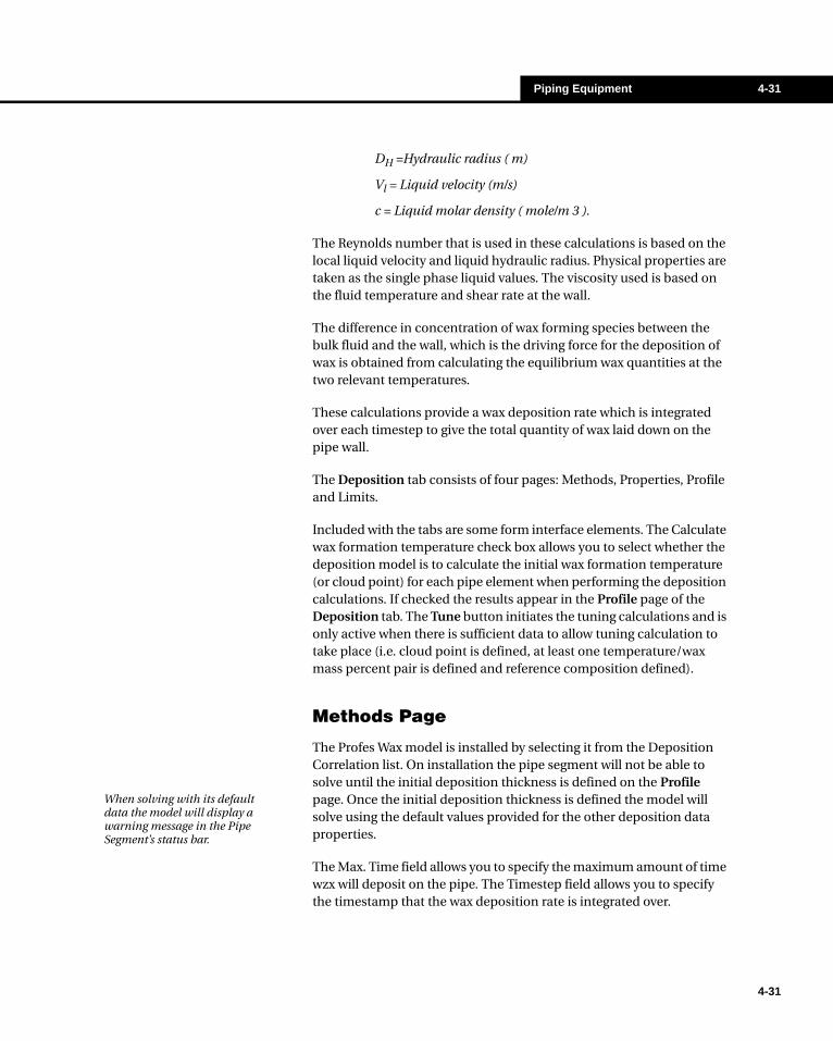
Piping Equipment 4-31
DH =Hydraulic radius ( m)
Vl = Liquid velocity (m/s)
c = Liquid molar density ( mole/m 3 ).
The Reynolds number that is used in these calculations is based on the local liquid velocity and liquid hydraulic radius. Physical properties are taken as the single phase liquid values. The viscosity used is based on the fluid temperature and shear rate at the wall.
The difference in concentration of wax forming species between the bulk fluid and the wall, which is the driving force for the deposition of wax is obtained from calculating the equilibrium wax quantities at the two relevant temperatures.
These calculations provide a wax deposition rate which is integrated over each timestep to give the total quantity of wax laid down on the pipe wall.
The Deposition tab consists of four pages: Methods, Properties, Profile and Limits.
Included with the tabs are some form interface elements. The Calculate wax formation temperature check box allows you to select whether the deposition model is to calculate the initial wax formation temperature (or cloud point) for each pipe element when performing the deposition calculations. If checked the results appear in the Profile page of the Deposition tab. The Tune button initiates the tuning calculations and is only active when there is sufficient data to allow tuning calculation to take place (i.e. cloud point is defined, at least one temperature/wax mass percent pair is defined and reference composition defined).
Methods Page
The Profes Wax model is installed by selecting it from the Deposition Correlation list. On installation the pipe segment will not be able to solve until the initial deposition thickness is defined on the Profile page. Once the initial deposition thickness is defined the model will solve using the default values provided for the other deposition data properties.
The Max. Time field allows you to specify the maximum amount of time wzx will deposit on the pipe. The Timestep field allows you to specify the timestamp that the wax deposition rate is integrated over.
When solving with its default data the model will display a warning message in the Pipe Segment’s status bar.
4-31

4-32 Pipe Segment
4-32
Click the View Method button to change the default data in the Profes Wax model and tune it to your specific application. The Profes Wax model correlation view consists of three tabs: Wax Data, Tuning Data and Ref. Comp.
Wax Data Tab
The Wax Data tab allows you to select the wax model to be used for the wax equilibrium calculations. The Wax Model drop down list provides you with Four thermodynamic models for wax formation: Chung,
Figure 4.19
Figure 4.20
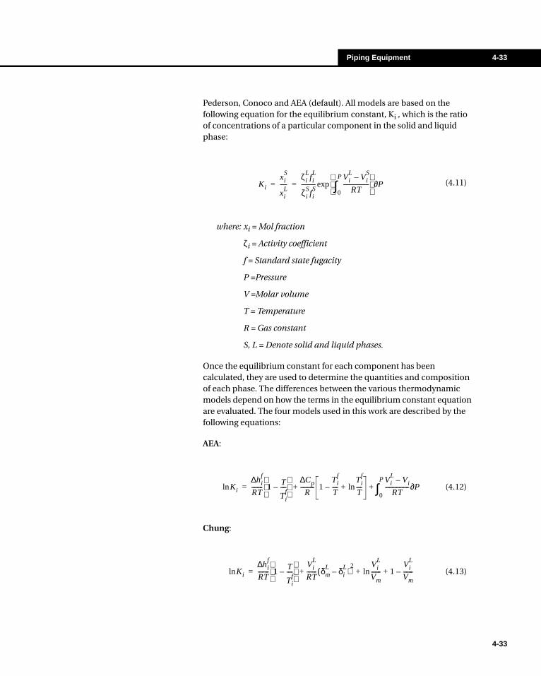
Piping Equipment 4-33
Pederson, Conoco and AEA (default). All models are based on the following equation for the equilibrium constant, Ki , which is the ratio of concentrations of a particular component in the solid and liquid phase:
where: xi = Mol fraction
ζi = Activity coefficient
f = Standard state fugacity
P =Pressure
V =Molar volume
T = Temperature
R = Gas constant
S, L = Denote solid and liquid phases.
Once the equilibrium constant for each component has been calculated, they are used to determine the quantities and composition of each phase. The differences between the various thermodynamic models depend on how the terms in the equilibrium constant equation are evaluated. The four models used in this work are described by the following equations:
AEA:
Chung:
(4.11)Ki
xiS
xiL
-----ζi
LfiL
ζiSfiS
----------Vi
LVi
S–
RT------------------
0
P
∫
P∂exp= =
(4.12)Kilnhi
f∆RT-------- 1
T
Tif
----– Cp∆
R---------- 1
Tif
T----–
Tif
T----ln+
ViL
Vi–
RT----------------- P∂
0
P
∫+ +=
(4.13)Kilnhi
f∆RT-------- 1
T
Tif
----– Vi
L
RT------- δm
L δiL
–( )2 Vi
L
Vm------- 1
ViL
Vm-------–+ln+ +=
4-33
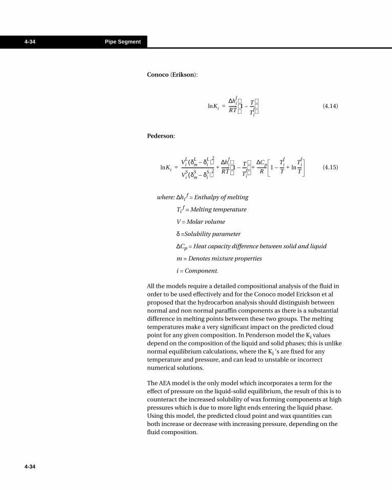
4-34 Pipe Segment
4-34
Conoco (Erikson):
Pederson:
where: ∆hi f = Enthalpy of melting
Ti f = Melting temperature
V = Molar volume
δ =Solubility parameter
∆Cp = Heat capacity difference between solid and liquid
m = Denotes mixture properties
i = Component.
All the models require a detailed compositional analysis of the fluid in order to be used effectively and for the Conoco model Erickson et al proposed that the hydrocarbon analysis should distinguish between normal and non normal paraffin components as there is a substantial difference in melting points between these two groups. The melting temperatures make a very significant impact on the predicted cloud point for any given composition. In Penderson model the Ki values depend on the composition of the liquid and solid phases; this is unlike normal equilibrium calculations, where the Ki ’s are fixed for any temperature and pressure, and can lead to unstable or incorrect numerical solutions.
The AEA model is the only model which incorporates a term for the effect of pressure on the liquid-solid equilibrium, the result of this is to counteract the increased solubility of wax forming components at high pressures which is due to more light ends entering the liquid phase. Using this model, the predicted cloud point and wax quantities can both increase or decrease with increasing pressure, depending on the fluid composition.
(4.14)Kilnhi
f∆RT-------- 1
T
Tif
----–
=
(4.15)KilnVi
L δmL δi
L–( )
2
ViS δm
S δiS
–( )2
--------------------------------hi
f∆RT--------+ 1
T
Tif
----– Cp∆
R---------- 1
Tif
T----–
Tif
T----ln++=

Piping Equipment 4-35
The table allows you to select which components in the system are able to form wax. The default criteria for the components in this table are as follows:
• Components with a mole weight less than 140 or inorganic component types can never form wax. The check box for these components is set to a solid box that cannot be modified.
• Hydrocarbon component types will form wax. The check box is automatically selected for these components, but you can deactivate it. Note hypothetical components generally fall into this category.
• Other organic component types will not form wax. The check box is inactive but you can activate it.
The ability to select whether a particular component forms wax gives you additional control when defining the wax formation characteristics of a system. For example you can define two hypothetical components with common properties and by setting one as a wax former you could vary the quantity of wax produced in the boiling range covered by the hypotheticals by varying their proportions.
Tuning Data Tab
The Tuning Data tab allows you to define the observed wax formation characteristics of a system to tune the wax model.
Figure 4.21
4-35

4-36 Pipe Segment
4-36
The Cloud Point input field allows you to specify the temperature at which the first wax appears i.i. the phase transition temperature between single liquid phase and the two phase wax/liquid mixture.
The table of Temperature vs. Wax Mass Percent allows you to define the quantity of wax deposit observed as a function of temperature. New points can be added to the table in any order, they will be sorted by temperature when the tuning process is run. To run the tuning calculations a minimum of one pair of data points is required. Up to 10 pairs of data points may be supplied.
Calculated values for the Cloud Point and Wax Mass Percent will be displayed in the calculated column after the tuning process is run.
Ref Comp Tab
The Ref Comp tab allows you to specify the reference composition of the fluid in your pipe segment.
The composition is entered in a table as either a mole or mass fraction depending on which radio button is selected. The Normalise button allows you to normalise the composition entered and setting any unspecified fractions to zero.
Figure 4.22
To remove a point from the table both the temperature and the wax mass percent values must be deleted.

Piping Equipment 4-37
Tuning Process
The tuning process is a series of calculations that is initiated as a task by clicking the Tune button. The first step validates the tuning data supplied as follows:
• that there is at least one component identified as a wax former• a valid reference composition has been entered• sorting the pairs of temperature/wax mass percent in order of
descending temperature• ensure cloud point temperature is greater than any
temperature in table of temperature/wax mass percent pairs
If any problem is found the tuning process stops and an appropriate error message is displayed on the tuning status bar.
If the tuning data is valid then the tuning process first does a VLE flash at 15C and 100 kPa to calculate the liquid composition of the reference stream. This is used as the base composition for all subsequent tuning calculations. If a liquid phase cannot be found in the reference stream at these conditions the tuning calculations fail.
The tuning process then continues using an iterative least squares solution method. Progress of the tuning process is output to the main HYSYS status bar. When complete the tuning process checks for convergence and displays the result on the tuning status bar. If the tuning process converged then the calculated results on the Tuning data tab are updated. If the tuning process failed to converge the tuning parameters are not updated and the calculated results are not updated.
There are 3 tuning parameters available for the Chung, Pederson and Conoco wax models and 4 tuning parameters for the AEA model. The tuning process will only attempt to tune as many parameters as is possible from the supplied data i.e. cloud point + one pair of temperature/wax percent data will allow tuning of 2 parameters - more pairs of temperature/wax percent data points are required to tune additional parameters. In cases where an attempt to tune 3 or 4 parameters fails to converge, a second tuning attempt is made automatically for just 2 tuning parameters.
The convergence of the tuning process is checked by looking at the cloud point result since this is the most critical parameter. Generally convergence will be achieved when there are one or two pairs of temperature/wax percent data. Given the emphasis placed on achieving the cloud point the calculated results for wax percent can often show greater errors, particularly when there are multiple temperature/wax percent points.
4-37
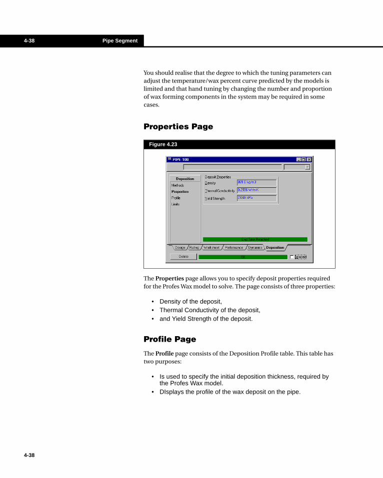
4-38 Pipe Segment
4-38
You should realise that the degree to which the tuning parameters can adjust the temperature/wax percent curve predicted by the models is limited and that hand tuning by changing the number and proportion of wax forming components in the system may be required in some cases.
Properties Page
The Properties page allows you to specify deposit properties required for the Profes Wax model to solve. The page consists of three properties:
• Density of the deposit,• Thermal Conductivity of the deposit,• and Yield Strength of the deposit.
Profile Page
The Profile page consists of the Deposition Profile table. This table has two purposes:
• Is used to specify the initial deposition thickness, required by the Profes Wax model.
• DIsplays the profile of the wax deposit on the pipe.
Figure 4.23
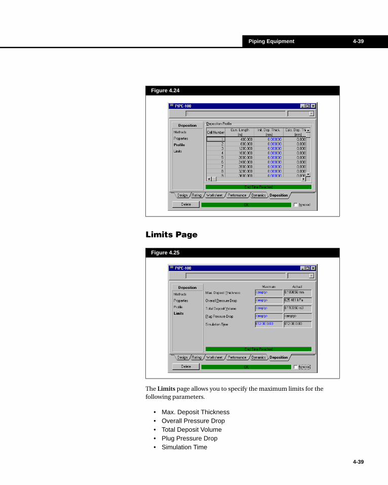
Piping Equipment 4-39
4-39
Limits Page
The Limits page allows you to specify the maximum limits for the following parameters.
• Max. Deposit Thickness• Overall Pressure Drop• Total Deposit Volume• Plug Pressure Drop• Simulation Time
Figure 4.24
Figure 4.25

4-40 Pipe Segment
4-40
4.2.8 Pipe ExampleThis example will illustrate the use of the PIPE SEGMENT, where the flowrate is unknown.
1. Create the Feed stream using the Peng Robinson property method and the required components.
2. Create the stream Feed with the following specifications:
3. Install the PIPE SEGMENT with the following
Property Package Components
Peng Robinson Methane, Ethane, Propane, i-Butane, n-Butane, i-Pentane, CO2, H2O
MATERIAL STREAM [Feed]
Tab [Page] Input Area Entry
Worksheet [Conditions]
Temperature [C] 50.0000
Pressure [kPa] 3000.00
Worksheet [Composition]
Methane 0.8800
Ethane 0.0600
Propane 0.0300
i-Butane 0.0050
n-Butane 0.0050
i-Pentane 0.0020
CO2 0.0100
H2O 0.0080
PIPE SEGMENT [Pipe-100]
Tab [Page] Input Area Entry
Design [Connections]
Feed Feed
Product Product
Energy Duty
Design [Parameters]Pipe Flow Correlation Beggs and Brill
Delta P [kPa] 1000.0000

Piping Equipment 4-41
4. On the Sizing page of the Ratings tab, add one segment to the unit operation by pressing the Add Segment button. Specify the Fitting/Pipe, the Length, the Elevation and the Increments as shown below.
5. Press the View Segment button to select a 101.6 mm (4-inch) nominal diameter Schedule 40 pipe. The Outer Diameter and Inner Diameter will be calculated by HYSYS.
6. Specify a Heat Loss of 5000 kJ/h in the Heat Transfer page of the Rating tab. Once you do this, the PIPE SEGMENT begins its calculations.
Results
Examine the results on the Profile page in the Performance tab by pressing the View Profile button. The Table page is shown:
The calculated flowrate of the fluid through the PIPE SEGMENT can be seen on the Worksheet page. A molar flow rate of 761.56 kgmole/hr is calculated for a 1000 kPa pressure drop through 500 m of 4-in. mild steel, Schedule 40 pipe.
Tab [Page] Input Area Entry
Rating [Sizing]
Fitting/Pipe Pipe
Length 500 m
Elevation Change 0 m
Material Mild Steel
Increments 10
Figure 4.26
4-41
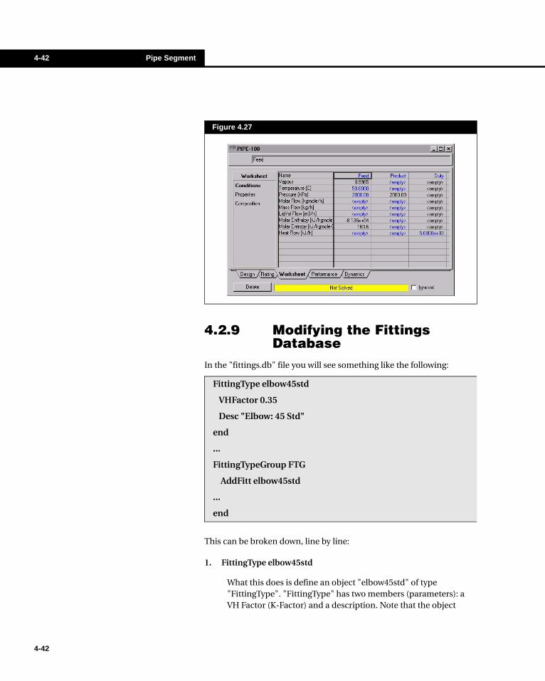
4-42 Pipe Segment
4-42
4.2.9 Modifying the Fittings Database
In the "fittings.db" file you will see something like the following:
This can be broken down, line by line:
1. FittingType elbow45std
What this does is define an object "elbow45std" of type "FittingType". "FittingType" has two members (parameters): a VH Factor (K-Factor) and a description. Note that the object
Figure 4.27
FittingType elbow45std
VHFactor 0.35
Desc "Elbow: 45 Std"
end
...
FittingTypeGroup FTG
AddFitt elbow45std
...
end
Piping Equipment 4-43
name "elbow45std" is only an internal name; it doesn’t appear in any lists or windows.
2. VHFactor 0.35
This is the K-Factor for the fitting. When you add a fitting to the fittings list, this is the number that is put in the K-Factor column.
3. Desc "Elbow: 45 Std"
This assigns a label (description) to the fitting "elbow45std". It is this label that is used in the fittings window to select fittings.
4. end
This tells HYSYS that the description of "elbow45std" is done.
So, you have a definition of a fitting. But, that’s not quite enough. All the fittings are gathered into one group - a "FittingTypeGroup"- to make it easier for HYSYS to determine what should go where.
1. FittingTypeGroup FTG
Same as line 1 above. This defines an object "FTG" of type "FittingTypeGroup". "FTG" can have many parameters, but they must all be of the same type - FittingType. The FittingTypeGroup is like a container for all the pipe fittings.
2. AddFitt elbow45std
This adds the previously defined fitting to the group. Note that the fitting MUST be defined before it is added to the group. All new fittings should be added last in the database file. When the fittings appear in the drop down list, they are sorted alphabetically by their Desc parameter.
3. end
This tells HYSYS that you have added all the fittings you want to the fitting group.
Note that HYSYS will not automatically put fittings in the group just because they are defined beforehand. For example, if we had defined "elbow45std" as above, but forgot to add it to the fittings group, there would be no way to access it in the fittings window.
New fittings should be added as the last entry in the database.
4-43
4-44 Tee
4-44
Also, the "end" command is very important. If you forget to put an "end" in somewhere in the middle of the fittings.db file, you will get errors that may or may not tell you what is actually wrong.
So, now you can add your own fitting. Open the "fitting.db" file in an ASCII editor and move somewhere in the middle of the file (but make sure that you are above the definition of the fittings group).
Now, add the following lines:
FittingType loopdeloop
VHFactor 10.0
Desc "Loop-de-loop!"
end
You have now created a fitting. Note that you don’t have to indent the VHFactor and Desc lines, it just makes for neater and easier to read files. Now, the fitting is added to the fittings group.
Find the line in the file that says "FittingTypeGroup FTG". Now, go anywhere between this line and the "end" line and type the following:
AddFitt loopdeloop
Now all you have to do is run HYSYS and make a pipe segment. The new fitting "Loop-de-loop!" will appear in the fittings drop down list, and if you add a "Loop-de-loop!" to the fittings list, it will come up with a K-Factor of 10.0.
To take out the fitting, just delete the lines that were previously added.
4.3 TeeThe Tee operation splits one feed stream into multiple product streams with the same conditions and composition as the feed stream, and is used for simulating pipe tees and manifolds.
To install the Tee operation, press F12 and choose Tee from the Unit Ops view or select the Tee button in the Object Palette. To ignore the Tee operation during calculations, activate the Ignored check box. HYSYS will disregard the operation until you clear the check box.
Tee Button

Piping Equipment 4-45
4.3.1 Design TabThe Design tab provides access to four pages: the Connections, Parameters, User Variables, and Notes page.
Connections Page
On the Connections page, provide the name of the Feed stream as well as any number of Product streams, all of which will be assigned the conditions and composition of the Feed. The only difference among the Products are the flow rates, determined by the flow ratios which you specify on the Parameters page (Steady-State mode) or the outlet valve openings you specify on the Dynamics page (Dynamic mode).
Parameters Page
For steady-state calculations, provide the desired flow ratio (the ratio of the outlet stream flow to the total inlet flow). A flow ratio is generally between 0 and 1; however, a ratio greater than one may be given. In that case, at least one of the outlet streams will have a negative flow ratio and a negative flow (backflow). For N outlet streams attached to the TEE, you must provide N-1 flow ratios. HYSYS will then calculate the unknown stream flow ratio and the outlet flow rates.
Figure 4.28
4-45
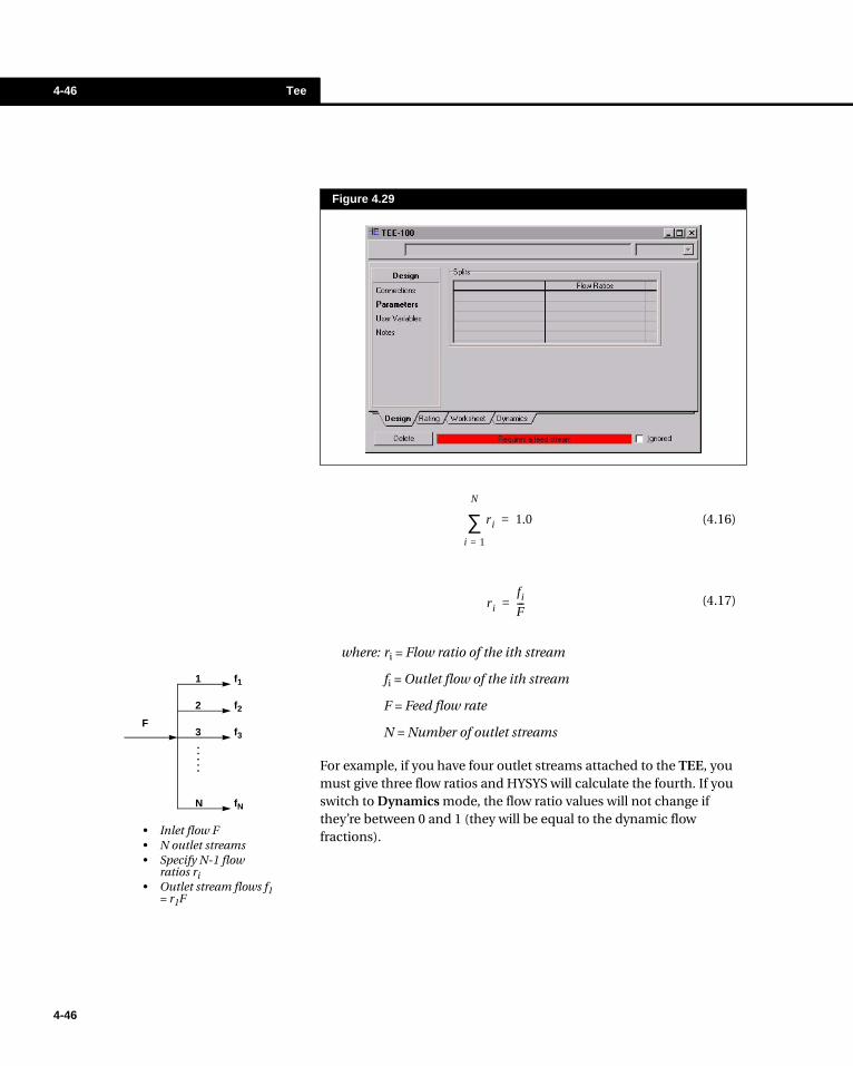
4-46 Tee
4-46
where: ri = Flow ratio of the ith stream
fi = Outlet flow of the ith stream
F = Feed flow rate
N = Number of outlet streams
For example, if you have four outlet streams attached to the TEE, you must give three flow ratios and HYSYS will calculate the fourth. If you switch to Dynamics mode, the flow ratio values will not change if they’re between 0 and 1 (they will be equal to the dynamic flow fractions).
Figure 4.29
(4.16)
(4.17)
ri
i 1=
N
∑ 1.0=
ri
fi
F---=
F
1
3
2
. . . . .
N
f1
f2
f3
fN
• Inlet flow F• N outlet streams• Specify N-1 flow
ratios ri• Outlet stream flows f1
= r1F
Piping Equipment 4-47
User Variables Page
The User Variables page allows the user to create and implement variables in the HYSYS simulation case. For more information on implementing the User Variables option, see the User Variables chapter in the Customization Guide.
Notes Page
The Notes page provides a text editor where you can record any comments or information regarding the Tee operation or pertaining to your simulation, in general.
4.3.2 Ratings TabYou are unable to specify any rating information for the TEE operation in HYSYS.Process.
4.3.3 Worksheet TabThe Worksheet tab contains a summary of the information contained in the stream property view for all the streams attached to the unit operation. The Conditions, Properties, and Composition pages contain selected information from the corresponding pages of the Worksheet tab for the stream property view. The PF Specs page contains a summary of the stream property view Dynamics tab.
4.3.4 Dynamics TabIf you are working exclusively in Steady State mode, you are not required to change any information on the pages accessible through this tab. For more information on running the Tee operation in Dynamics mode, see the Dynamic Modeling guide for further details.
4-47

4-48 Valve
4-48
4.4 ValveHYSYS performs a material and energy balance on the inlet and exit streams of the Valve operation. HYSYS performs a flash calculation based on equal material and enthalpy between the two streams. It is assumed that the valve operation is isenthalpic.
The following is a list of variables that may be specified by the user in the Valve operation. A total of three specifications are required before the valve operation will solve. At least one temperature specification and one pressure specification are required. HYSYS will calculate the other two unknowns:
• Inlet temperature• Inlet pressure• Outlet temperature• Outlet pressure• Valve Pressure Drop
To install the Valve operation, press F12 and choose Valve from the Unit Ops view or select the Valve button in the Object Palette.
To ignore the Valve operation during calculations, activate the Ignored check box. HYSYS will disregard the operation until you clear the check box.
Valve Button

Piping Equipment 4-49
4.4.1 Design TabThe Design tab provides access to four pages: the Connections, Parameters, User Variables, and Notes page.
Connections Page
The Connections page allows provide the name of the Valve, as well as the Feed and Product stream names.
Parameters Page
The pressure drop of the Valve operation may be specified on the Parameters page.
User Variables Page
The User Variables page allows the user to create and implement variables in the HYSYS simulation case. For more information on implementing the User Variables option, see the User Variables chapter in the Customization Guide.
Figure 4.30
4-49

4-50 Valve
4-50
Notes Page
The Notes page provides a text editor where you can record any comments or information regarding the VALVE operation or pertaining to your simulation, in general.
4.4.2 Ratings TabIf you are working exclusively in Steady State mode, you are not required to change any information on the pages accessible through this tab. For more information on running the VALVE operation in Dynamics mode, see the Dynamic Modeling guide for further details.
4.4.3 Worksheet TabThe Worksheet tab contains a summary of the information contained in the stream property view for all the streams attached to the unit operation. The Conditions, Properties, and Composition pages contain selected information from the corresponding pages of the Worksheet tab for the Stream property view. The PF Specs page contains a summary of the stream property view Dynamics tab.
4.4.4 Dynamics TabIf you are working exclusively in Steady State mode, you are not required to change any information on the pages accessible through this tab. For more information on running the VALVE operation in Dynamics mode, see the Dynamic Modeling guide for further details.
4.4.5 Valve ExampleThis example will illustrate the use of the VALVE operation. In this case, the temperature and pressure of the Feed to the valve is specified.
1. Create the Feed stream using the Peng Robinson property method and the required components.
Property Package Components
Peng Robinson Propane, Propene
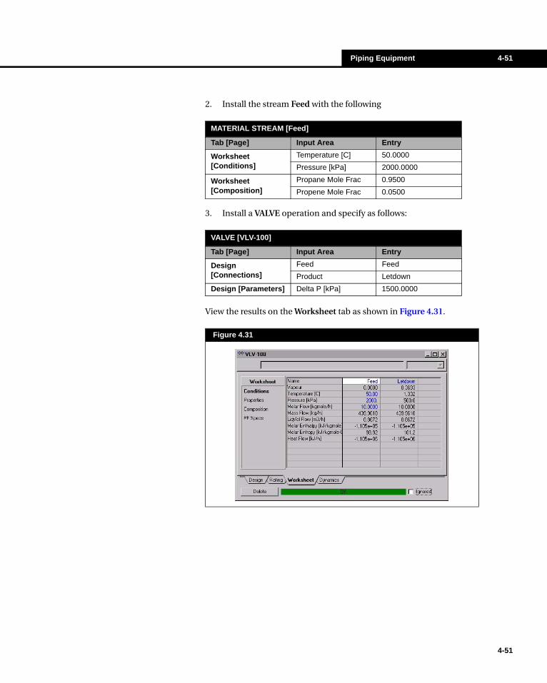
Piping Equipment 4-51
2. Install the stream Feed with the following
3. Install a VALVE operation and specify as follows:
View the results on the Worksheet tab as shown in Figure 4.31.
MATERIAL STREAM [Feed]
Tab [Page] Input Area Entry
Worksheet [Conditions]
Temperature [C] 50.0000
Pressure [kPa] 2000.0000
Worksheet [Composition]
Propane Mole Frac 0.9500
Propene Mole Frac 0.0500
VALVE [VLV-100]
Tab [Page] Input Area Entry
Design [Connections]
Feed Feed
Product Letdown
Design [Parameters] Delta P [kPa] 1500.0000
Figure 4.31
4-51
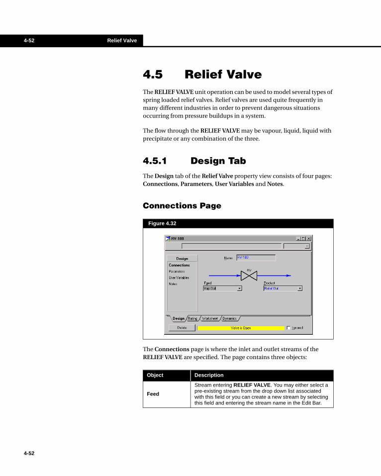
4-52 Relief Valve
4-52
4.5 Relief ValveThe RELIEF VALVE unit operation can be used to model several types of spring loaded relief valves. Relief valves are used quite frequently in many different industries in order to prevent dangerous situations occurring from pressure buildups in a system.
The flow through the RELIEF VALVE may be vapour, liquid, liquid with precipitate or any combination of the three.
4.5.1 Design TabThe Design tab of the Relief Valve property view consists of four pages: Connections, Parameters, User Variables and Notes.
Connections Page
The Connections page is where the inlet and outlet streams of the RELIEF VALVE are specified. The page contains three objects:
Figure 4.32
Object Description
Feed
Stream entering RELIEF VALVE. You may either select a pre-existing stream from the drop down list associated with this field or you can create a new stream by selecting this field and entering the stream name in the Edit Bar.

Piping Equipment 4-53
Parameters Page
The Parameters page contains only two fields:
User Variables Page
The User Variables page allows the user to create and implement variables in the HYSYS simulation case. For more information on implementing the User Variables option, see the User Variables chapter of the Customization Guide.
Product
RELIEF VALVE exit stream. Like the Feed field, you may either select an existing stream from the associated drop down or you can create a new stream by selecting the field and entering the stream name in the Edit Bar.
Name
The name of the RELIEF VALVE. HYSYS will provide a default designation for the unit operation, however, you may edit this name at any time by entering a new name in this field.
Object Description
Figure 4.33
Object Description
Opening Pressure The pressure at which the relief valve will begin to open.
Full Open Pressure The pressure at which the relief valve is fully open.
4-53
4-54 Relief Valve
4-54
Notes Page
The Notes page provides a text editor where you can record any comments or information regarding the RELIEF VALVE or pertaining to your simulation, in general.
4.5.2 Ratings TabIf you are working exclusively in Steady State mode, you are not required to change any information on the pages accessible through this tab. For more information on running the RELIEF VALVE operation in Dynamics mode, see the Dynamic Modeling guide for further details.
4.5.3 Worksheet TabThe Worksheet tab contains a summary of the information contained in the stream property view for all the streams attached to the unit operation. The Conditions, Properties, and Composition pages contain selected information from the corresponding pages of the Worksheet tab for the Stream property view. The PF Specs page contains a summary of the Stream property view Dynamics tab.
4.5.4 Dynamics TabIf you are working exclusively in Steady State mode, you are not required to change any information on the pages accessible through this tab. For more information on running the RELIEF VALVE operation in Dynamics mode, see the Dynamic Modeling guide for further details.
4.5.5 Relief Valve ExampleThis example illustrates the use of a RELIEF VALVE with regards to a simple storage tank in Steady State mode.
1. Create a new case using the Peng Robinson Property Package and add the following components.
Property Package Components
Peng Robinson H2O

Piping Equipment 4-55
2. Create and specify the stream Feed with the following conditions and composition.
3. Now add a SEPARATOR to the Flowsheet with the following specifications:
4. The last unit operation you will require is the RELIEF VALVE. To add a RELIEF VALVE you can either press F12 and add one from the Unit Ops dialogue or select the Relief Valve button from the Object Palette.
5. Fill out the Design tab of Relief Valve property view as shown in the following table.
6. On the Worksheet tab of the Relief Valve property view, set the pressure of the Relief-Out stream to 101.325 kPa.
7. The system is now fully specified.The status bar at the bottom of the Relief Valve property view should be red and display the message: Material Flows into closed relief valve. The Relief-Out stream should remain unsolved.
The valve should be closed as the vessel pressure is not high enough for the Relief Valve to open.
MATERIAL STREAM [Feed]
Tab [Page] Input Area Entry
Worksheet [Conditions]
Vapour Fraction 0
Pressure [kPa] 2000.0000
Mass Flow [kg/hr] 1
Worksheet [Composition]
H2O Mole Frac 1.0
SEPARATOR [Sep]
Tab [Page] Input Area Entry
Design [Connections]Feed Feed
Liquid Outlet Relief-In
Design [Parameters]Pressure Drop 0 psia
Type Tank
Relief Valve Button
RELIEF VALVE [RV-100]
Tab [Page] Input Area Entry
Design [Connections]
Feed Relief-In
Product Relief-Out
Design [Parameters]Opening Pressure 150 kPa
Full Open Pressure 200 kPa
4-55
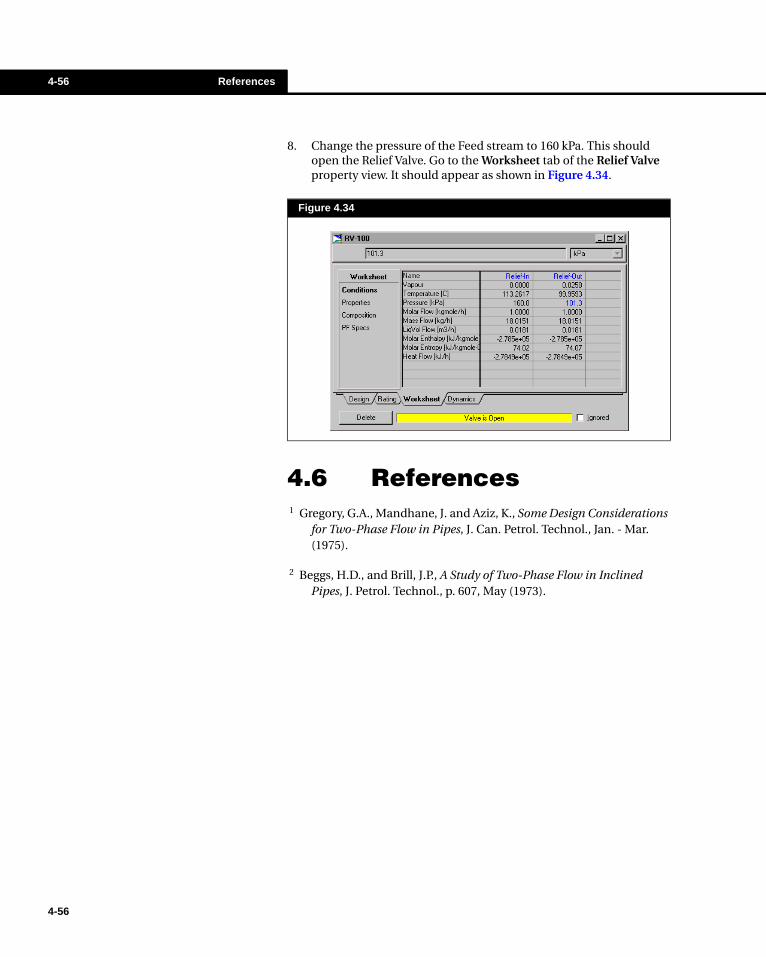
4-56 References
4-56
8. Change the pressure of the Feed stream to 160 kPa. This should open the Relief Valve. Go to the Worksheet tab of the Relief Valve property view. It should appear as shown in Figure 4.34.
4.6 References 1 Gregory, G.A., Mandhane, J. and Aziz, K., Some Design Considerations
for Two-Phase Flow in Pipes, J. Can. Petrol. Technol., Jan. - Mar. (1975).
2 Beggs, H.D., and Brill, J.P., A Study of Two-Phase Flow in Inclined Pipes, J. Petrol. Technol., p. 607, May (1973).
Figure 4.34
Rotating Equipment 5-1
5 Rotating Equipment
5-1
5.1 Compressor/Expander................................................................................. 3
5.1.1 Theory...................................................................................................... 45.1.2 Design Tab ............................................................................................... 85.1.3 Rating Tab...............................................................................................115.1.4 Worksheet Tab ....................................................................................... 145.1.5 Performance Tab.................................................................................... 145.1.6 Dynamics Tab ........................................................................................ 155.1.7 Compressor Example............................................................................. 15
5.2 Reciprocating Compressor ....................................................................... 18
5.2.1 Theory.................................................................................................... 195.2.2 Design Tab ............................................................................................. 235.2.3 Rating Tab.............................................................................................. 255.2.4 Worksheet Tab ....................................................................................... 265.2.5 Performance Tab.................................................................................... 265.2.6 Dynamics Tab ........................................................................................ 275.2.7 Reciprocating Compressor Example...................................................... 27
5.3 Pump ........................................................................................................... 29
5.3.1 Theory.................................................................................................... 305.3.2 Design Tab ............................................................................................. 325.3.3 Rating Tab.............................................................................................. 345.3.4 Worksheet Tab ....................................................................................... 345.3.5 Performance Tab.................................................................................... 345.3.6 Dynamics Tab ........................................................................................ 345.3.7 Pump Example....................................................................................... 35

5-2
5-2

Rotating Equipment 5-3
5.1 Compressor/ExpanderThe Compressor operation is used to increase the pressure of an inlet gas stream. Depending on the information supplied, the Compressor calculates either a stream property (pressure or temperature) or a compression efficiency.
The Expander operation is used to decrease the pressure of a high pressure inlet gas stream to produce an outlet stream with low pressure and high velocity. An expansion process involves converting the internal energy of the gas to kinetic energy and finally to shaft work. The Expander will calculate either a stream property or an expansion efficiency.
There are several methods for the Compressor (Expander) to solve, depending on what information has been supplied and whether or not you are using curves. In general, the solution is a function of flow, pressure change, applied energy and efficiency. The Compressor/Expander provides a great deal of flexibility with respect to what you can supply and what it will then calculate. You must ensure that you do not enable too many of the solution options or inconsistencies may result.
Typical Solution Methods
The thermodynamic principles governing the Compressor and Expander operations are the same, but the direction of the energy stream flow is opposite. Compression requires energy, while expansion releases energy.
To install the Compressor operation, press F12 and select Compressor from the UnitOps view or select the Compressor button in the Object Palette. The Expander operation is installed similarly.
Without Curves With Curves
1. Flow rate and inlet pressure are known.
2. Specify outlet pressure.
3. Specify either Adiabatic or Polytropic efficiency.
4. HYSYS will calculate the required energy, outlet temperature and other efficiency.
1. Flow rate and inlet pressure are known.
2. Specify operating speed.
3. HYSYS uses curves to determine efficiency and head.
4. HYSYS calculates outlet pressure, temperature, and applied duty.
1. Flow rate and inlet pressure are known.
2. Specify efficiency and duty.
3. HYSYS will calculate outlet pressure, temperature, and other efficiency.
1. Flow rate, inlet pressure, and efficiency are known.
2. HYSYS interpolates curves to determine operating speed and head.
3. HYSYS calculates outlet pressure, temperature, and applied duty.
Compressor Button
Expander Button
5-3
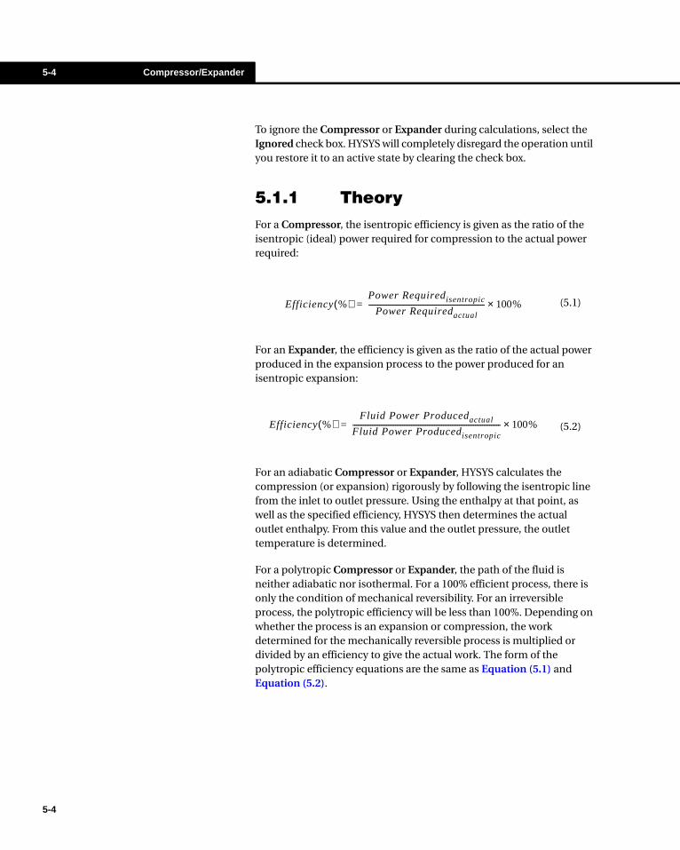
5-4 Compressor/Expander
5-4
To ignore the Compressor or Expander during calculations, select the Ignored check box. HYSYS will completely disregard the operation until you restore it to an active state by clearing the check box.
5.1.1 TheoryFor a Compressor, the isentropic efficiency is given as the ratio of the isentropic (ideal) power required for compression to the actual power required:
For an Expander, the efficiency is given as the ratio of the actual power produced in the expansion process to the power produced for an isentropic expansion:
For an adiabatic Compressor or Expander, HYSYS calculates the compression (or expansion) rigorously by following the isentropic line from the inlet to outlet pressure. Using the enthalpy at that point, as well as the specified efficiency, HYSYS then determines the actual outlet enthalpy. From this value and the outlet pressure, the outlet temperature is determined.
For a polytropic Compressor or Expander, the path of the fluid is neither adiabatic nor isothermal. For a 100% efficient process, there is only the condition of mechanical reversibility. For an irreversible process, the polytropic efficiency will be less than 100%. Depending on whether the process is an expansion or compression, the work determined for the mechanically reversible process is multiplied or divided by an efficiency to give the actual work. The form of the polytropic efficiency equations are the same as Equation (5.1) and Equation (5.2).
(5.1)Efficiency %( )Power Requiredisentropic
Power Requiredactual----------------------------------------------------------------- 100%×=
(5.2)Efficiency %( )Fluid Power Producedactual
Fluid Power Producedisentropic----------------------------------------------------------------------------------- 100%×=

Rotating Equipment 5-5
Note that all intensive quantities are determined thermodynamically, using the specified Property Package. In general, the work for a mechanically reversible process can be determined from:.
As with any unit operation, the calculated information depends on the information which is supplied by the user. In the case where the inlet and outlet pressures and temperatures of the gas are known, the ideal (isentropic) power of the Operation is calculated using one of the above equations, depending on the compressor or expander type. The actual power is equivalent to the heat flow (enthalpy) difference between the inlet and outlet streams.
For the Compressor:
where the efficiency of the Compressor is then determined as the ratio of the isentropic power to the actual power required for compression.
For the Expander:
The efficiency of the Expander is then determined as the ratio of the actual power produced by the gas to the isentropic power.
In the case where the inlet pressure, the outlet pressure, the inlet temperature and the efficiency are known, the isentropic power is once again calculated using the appropriate equation. The actual power required by the Compressor (enthalpy difference between the inlet and outlet streams) is calculated by dividing the ideal power by the compressor efficiency. The outlet temperature is then rigorously determined from the outlet enthalpy of the gas using the enthalpy expression derived from the property method being used. For an isentropic compression or expansion (100% efficiency), the outlet temperature of the gas will always be lower than the outlet temperature for a real compression or expansion.
(5.3)W V Pd∫=
Power Requiredactual = Heat Flowoutlet - Heat Flowinlet (5.4)
Power Producedactual = Heat Flowinlet - Heat Flowoutlet (5.5)
5-5

5-6 Compressor/Expander
5-6
Equations Used
If the Compressor is selected, the compressor equations are used. If the Expander is selected, the expander equations are used.
Compressor Efficiencies
The Adiabatic and Polytropic Efficiencies are included in the compressor calculations. An isentropic flash (Pin and Entropyin) is performed internally to obtain the ideal (isentropic) properties.
Expander Efficiencies
For an expander, the efficiencies are parts of the expander calculations, and an isentropic flash is performed as well. The flash is done on the expander fluid, and the results are not stored.
EFFICIENCIES Compressor Expander
Adiabatic
Polytropic
where: where:
where: H = Mass Enthalpy
out = Product Discharge
in = Feed Stream
P = Pressure
ρ = Mass Density
n = Polytropic Exponent
k = Isentropic Exponent
Work Required ideal( )Work Required actual( )----------------------------------------------------------
Hout Hin–( )ideal( )
Hout Hin–( )actual( )
--------------------------------------------------------=Work Produced actual( )Work Produced ideal( )
------------------------------------------------------------Hout Hin–( )
actual( )Hout Hin–( )
ideal( )--------------------------------------------------------=
PoutPin
------------
n 1–n
------------
1–n
n 1–( )----------------
k 1–k
----------- ××
PoutPin
------------
k 1–k
-----------
1–
------------------------------------------------------------------------------------------------------------ AdiabaticEff×
PoutPin
------------
k 1–k
-----------
1–
PoutPin
------------
n 1–n
------------
1–n
n 1–( )----------------
k 1–k
----------- ××
------------------------------------------------------------------------------------------------------------ AdiabaticEff×
nPout Pin⁄( )log
ρout actual, ρin⁄( )log----------------------------------------------------------= n
Pout Pin⁄( )log
ρout actual, ρin⁄( )log----------------------------------------------------------=
kPout Pin⁄( )log
ρout ideal, ρin⁄( )log------------------------------------------------------= k
Pout Pin⁄( )log
ρout ideal, ρin⁄( )log------------------------------------------------------=
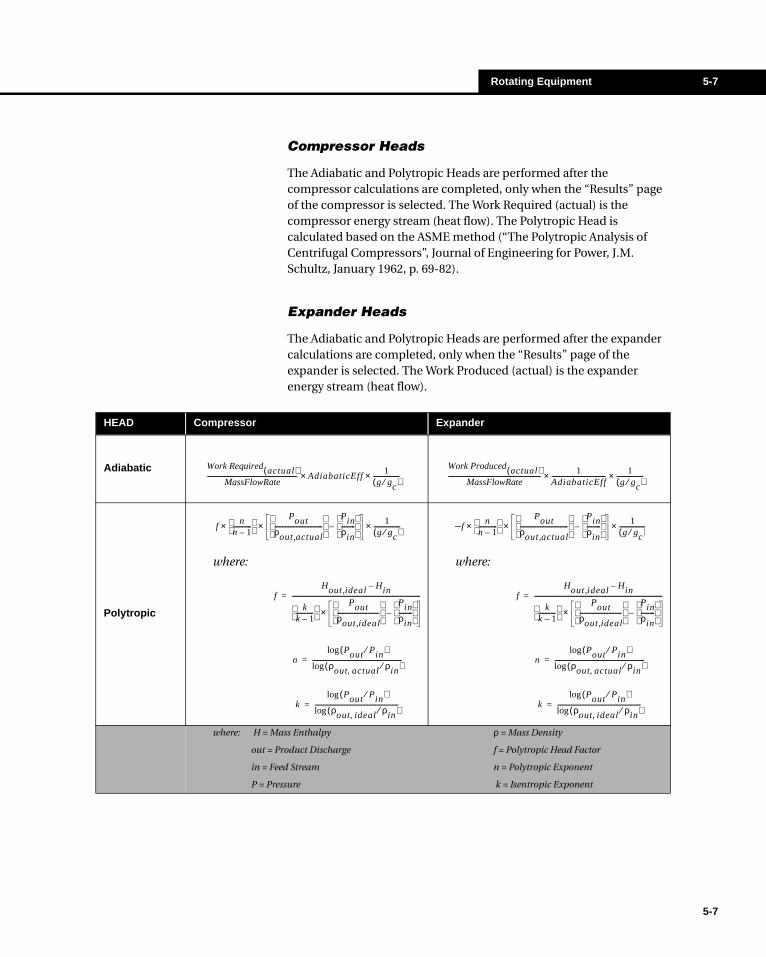
Rotating Equipment 5-7
Compressor Heads
The Adiabatic and Polytropic Heads are performed after the compressor calculations are completed, only when the “Results” page of the compressor is selected. The Work Required (actual) is the compressor energy stream (heat flow). The Polytropic Head is calculated based on the ASME method (“The Polytropic Analysis of Centrifugal Compressors”, Journal of Engineering for Power, J.M. Schultz, January 1962, p. 69-82).
Expander Heads
The Adiabatic and Polytropic Heads are performed after the expander calculations are completed, only when the “Results” page of the expander is selected. The Work Produced (actual) is the expander energy stream (heat flow).
HEAD Compressor Expander
Adiabatic
Polytropic
where: where:
where: H = Mass Enthalpy
out = Product Discharge
in = Feed Stream
P = Pressure
ρ = Mass Density
f = Polytropic Head Factor
n = Polytropic Exponent
k = Isentropic Exponent
Work Required actual( )MassFlowRate
---------------------------------------------------------- AdiabaticEff1
g gc⁄( )-----------------××
Work Produced actual( )MassFlowRate
------------------------------------------------------------1
AdiabaticEff-----------------------------------
1g gc⁄( )
-----------------××
fn
n 1–------------
Pout
ρout actual,-------------------------------
Pin
ρin---------
–×× 1g gc⁄( )
-----------------× fn
n 1–------------
Pout
ρout actual,-------------------------------
Pin
ρin---------
–××– 1g gc⁄( )
-----------------×
fHout ideal, Hin–
kk 1–-----------
Pout
ρout ideal,---------------------------
Pin
ρin---------
–×
-----------------------------------------------------------------------------------= fHout ideal, Hin–
kk 1–-----------
Pout
ρout ideal,---------------------------
Pin
ρin---------
–×
-----------------------------------------------------------------------------------=
nPout Pin⁄( )log
ρout actual, ρin⁄( )log----------------------------------------------------------= n
Pout Pin⁄( )log
ρout actual, ρin⁄( )log----------------------------------------------------------=
kPout Pin⁄( )log
ρout ideal, ρin⁄( )log------------------------------------------------------= k
Pout Pin⁄( )log
ρout ideal, ρin⁄( )log------------------------------------------------------=
5-7

5-8 Compressor/Expander
5-8
5.1.2 Design Tab
Connections Page
The Connections page, as shown in Figure 5.1, is for the Compressor. The information required on the Connections page of the Expander is identical; the only difference is that the expander icon is shown rather than the compressor icon.
On the Connections page, supply the operation name, as well as the names of the Inlet, Outlet and Energy Streams.
Parameters Page
The Parameters pages are identical for both the Compressor and Expander. The only difference is the icons are used to represent the operation and the ability to choose between a centrifugal and reciprocating compressor.
You may specify the duty of the attached energy stream on this page, or allow HYSYS to calculate it. The adiabatic and polytropic efficiencies are displayed as well.
Note that you may specify only one efficiency, either adiabatic or polytropic. If you specify one efficiency and a solution is obtained, HYSYS will then back calculate the other efficiency, using the calculated duty and stream conditions.
Figure 5.1
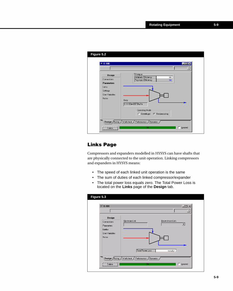
Rotating Equipment 5-9
Links Page
Compressors and expanders modelled in HYSYS can have shafts that are physically connected to the unit operation. Linking compressors and expanders in HYSYS means:
• The speed of each linked unit operation is the same• The sum of duties of each linked compressor/expander• The total power loss equals zero. The Total Power Loss is
located on the Links page of the Design tab.
Figure 5.2
Figure 5.3
5-9
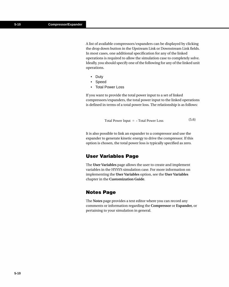
5-10 Compressor/Expander
5-10
A list of available compressors/expanders can be displayed by clicking the drop down button in the Upstream Link or Downstream Link fields. In most cases, one additional specification for any of the linked operations is required to allow the simulation case to completely solve. Ideally, you should specify one of the following for any of the linked unit operations.
• Duty• Speed• Total Power Loss
If you want to provide the total power input to a set of linked compressors/expanders, the total power input to the linked operations is defined in terms of a total power loss. The relationship is as follows:
It is also possible to link an expander to a compressor and use the expander to generate kinetic energy to drive the compressor. If this option is chosen, the total power loss is typically specified as zero.
User Variables Page
The User Variables page allows the user to create and implement variables in the HYSYS simulation case. For more information on implementing the User Variables option, see the User Variables chapter in the Customization Guide.
Notes Page
The Notes page provides a text editor where you can record any comments or information regarding the Compressor or Expander, or pertaining to your simulation in general.
(5.6)Total Power Input - Total Power Loss=
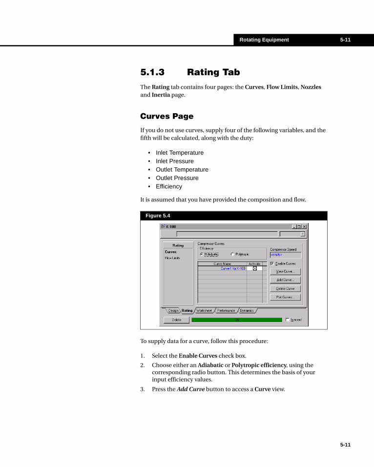
Rotating Equipment 5-11
5.1.3 Rating TabThe Rating tab contains four pages: the Curves, Flow Limits, Nozzles and Inertia page.
Curves Page
If you do not use curves, supply four of the following variables, and the fifth will be calculated, along with the duty:
• Inlet Temperature• Inlet Pressure• Outlet Temperature• Outlet Pressure• Efficiency
It is assumed that you have provided the composition and flow.
To supply data for a curve, follow this procedure:
1. Select the Enable Curves check box.
2. Choose either an Adiabatic or Polytropic efficiency, using the corresponding radio button. This determines the basis of your input efficiency values.
3. Press the Add Curve button to access a Curve view.
Figure 5.4
5-11
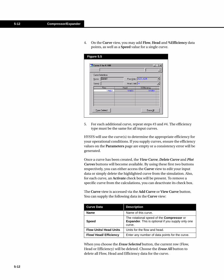
5-12 Compressor/Expander
5-12
4. On the Curve view, you may add Flow, Head and %Efficiency data points, as well as a Speed value for a single curve.
5. For each additional curve, repeat steps #3 and #4. The efficiency type must be the same for all input curves.
HYSYS will use the curve(s) to determine the appropriate efficiency for your operational conditions. If you supply curves, ensure the efficiency values on the Parameters page are empty or a consistency error will be generated.
Once a curve has been created, the View Curve, Delete Curve and Plot Curves buttons will become available. By using these first two buttons respectively, you can either access the Curve view to edit your input data or simply delete the highlighted curve from the simulation. Also, for each curve, an Activate check box will be present. To remove a specific curve from the calculations, you can deactivate its check box.
The Curve view is accessed via the Add Curve or View Curve button. You can supply the following data in the Curve view:
When you choose the Erase Selected button, the current row (Flow, Head or Efficiency) will be deleted. Choose the Erase All button to delete all Flow, Head and Efficiency data for the curve.
Figure 5.5
Curve Data Description
Name Name of this curve.
SpeedThe rotational speed of the Compressor or Expander. This is optional if you supply only one curve.
Flow Units/ Head Units Units for the flow and head.
Flow/ Head/ Efficiency Enter any number of data points for the curve.

Rotating Equipment 5-13
Single Curve
When you have a single curve, the following combinations of input will allow the operation to completely solve (assuming the feed composition and temperature are known):
• Inlet Pressure and Flow Rate• Inlet Pressure and Duty• Inlet Pressure and Outlet Pressure• Inlet Pressure and Efficiency corresponding to the Curve type
(e.g. - if the Curve is Adiabatic, provide an Adiabatic Efficiency).
Multiple Curves
If multiple curves have been installed and an operating speed is specified on the Parameters page, then only the curve with the corresponding speed will be used. Note that you can specify a speed that is different than the speeds given for the curves. For example, if you provide curves for two speeds (1000/min and 2000/min), and you specify a speed of 1500/min, HYSYS will interpolate between the two curves to obtain the solution. You must also provide an inlet pressure and one of flow rate, duty, outlet pressure or efficiency, as explained above.
HYSYS can calculate the appropriate speed based on your input. In this case, you need to provide the feed composition, pressure and temperature as well as two of the following four variables:
• Flow rate• Duty• Efficiency• Outlet Pressure
Once you provide the necessary information, the appropriate speed will be determined, and the other two variables will then be calculated.
Note that a Compressor may also be used to represent a Pump operation when a more rigorous pump calculation is required. The Pump operation in HYSYS assumes that the liquid is incompressible. Therefore, if you wish to pump a fluid near its critical point (where it becomes compressible), you may do so by representing the Pump with a Compressor. The Compressor operation takes into account the compressibility of the liquid, thus performing a more rigorous calculation.
Each curve is named and has an associated Activate check box. You can turn individual curves on and off.
5-13
5-14 Compressor/Expander
5-14
Flow Limits Page
If you are working exclusively in Steady State mode, you are not required to change any information on the pages accessible through this page. For more information on running the Compressor or Expander operations in Dynamic mode, see the Dynamic Modeling guide for further details.
Nozzle Page
If you are working exclusively in Steady State mode, you are not required to change any information on the pages accessible through this page. For more information on running the Compressor or Expander operations in Dynamic mode, see the Dynamic Modeling guide for further details.
Inertia Page
If you are working exclusively in Steady State mode, you are not required to change any information on this page. For more information on running the Compressor or Expander operations in Dynamic mode, see the Dynamic Modeling guide for further details.
5.1.4 Worksheet TabThe Worksheet tab contains a summary of the information contained in the stream property view for all the streams attached to the unit operation. The Conditions, Properties, and Composition pages contain selected information from the corresponding pages of the Worksheet tab for the stream property view. The PF Specs page contains a summary of the stream property view Dynamics tab.
5.1.5 Performance Tab
Results Page
On the Results page, you can view a table of calculated values for the Compressor/Expander:
• Adiabatic Head• Polytropic Head• Adiabatic Efficiency
Rotating Equipment 5-15
• Polytropic Efficiency• Duty• Polytropic Head Factor• Polytropic Exponent• Isentropic Exponent• Speed• Duty Loss• Total Effective Piston Displacement Volume• Total Effective Fractional Clearance Volume• Maximum Pressure Ratio• Lead in Compression• Load in Tension
5.1.6 Dynamics TabIf you are working exclusively in Steady State mode, you are not required to change any information on the pages accessible through this tab. For more information on running the Compressor and Expander unit operations in Dynamic mode, see the Dynamic Modeling guide.
5.1.7 Compressor ExampleA compressor will be modelled using efficiency curves. Consider the LP gas from an Oil Production facility as a FEED to a compressor station. In this problem, we will simply determine the efficiency, based on the flow rate of the feed stream.
1. Create a fluid package using the Sour PR property package and add the following components: H2O, H2S, CO2, C1, C2, C3, i-C4, and n-C4.
2. Install the stream FEED and define it as follows:
Property Package Components
Sour PR H2O, H2S, CO2, C1, C2, C3, i-C4, n-C4
MATERIAL STREAM [Feed]
Tab [Page] Input Area Entry
Worksheet [Conditions]
Temperature 69.0000 °C
Pressure 120.0000 kPa
Molar Flow 500.0000 kgmole/hr
5-15

5-16 Compressor/Expander
5-16
3. Install a Compressor unit operation with the following information:
4. On the Parameters page, delete the default Adiabatic Efficiency value. Both the Adiabatic and Polytropic efficiencies should read <empty> to avoid a consistency error or a compressor over specification.
5. Switch to the Rating tab, and open the Curves page.
6. Ensure that the Adiabatic radio button in the Efficiency group is selected.
7. Check the Enable Curves box, and press the Add Curve button.
8. Complete the curve as shown in Figure 5.6.
Worksheet [Composition]
H2O Mole Frac 0.2375
H2S Mole Frac 0.0727
CO2 Mole Frac 0.0607
C1 Mole Frac 0.0430
C2 Mole Frac 0.1072
C3 Mole Frac 0.2522
i-C4 Mole Frac 0.0765
n-C4 Mole Frac 0.1502
MATERIAL STREAM [Feed]
Tab [Page] Input Area Entry
Compressor [K-100]
Tab [Page] Input Area Entry
Design [Connections]
Inlet Feed
Outlet Out
Energy Comp Duty
Figure 5.6
It is not necessary to enter a Speed since only one curve is being used.
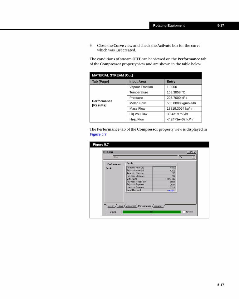
Rotating Equipment 5-17
9. Close the Curve view and check the Activate box for the curve which was just created.
The conditions of stream OUT can be viewed on the Performance tab of the Compressor property view and are shown in the table below.
The Performance tab of the Compressor property view is displayed in Figure 5.7.
MATERIAL STREAM [Out]
Tab [Page] Input Area Entry
Performance [Results]
Vapour Fraction 1.0000
Temperature 108.3858 °C
Pressure 203.7000 kPa
Molar Flow 500.0000 kgmole/hr
Mass Flow 18819.3064 kg/hr
Liq Vol Flow 33.4319 m3/hr
Heat Flow -7.2473e+07 kJ/hr
Figure 5.7
5-17
5-18 Reciprocating Compressor
5-18
5.2 Reciprocating Compressor
In Section 5.1 - Compressor/Expander a centrifugal compressor type is presented. The following section will now detail a reciprocating compressor. A reciprocating compressor is just another type of compressor used for applications where higher discharge pressures and lower flows are needed. It is known as a positive displacement type. Reciprocating compressors have a constant volume and variable head characteristics, as compared to the centrifugal compressor that has a constant head and variable volume.
In HYSYS, centrifugal and reciprocating compressors are accessed via the same compressor unit operation. However, the solution methods differ slightly as a reciprocating compressor does not require a compressor curve and required geometry data. The present capability of reciprocating compressors in HYSYS is focused on a single stage compressor with single or double acting piston. A typical solution method for a reciprocating compressor is as follows:
• Always start with a fully defined inlet stream, e.g. inlet pressure, temperature, flow rate and compositional data are known.
• Supply compressor geometry data like number of cylinders, cylinder type, bore, stroke and piston rod diameter. HYSYS provides default values too.
• Compressor performance data like adiabatic efficiency or polytropic efficiency and constant volumetric efficiency loss are supplied.
• HYSYS will calculate duty required, outlet temperature if the outlet pressure is specified.
To install the compressor operation, press F12 and select compressor from the unit Ops view or select the Compressor button in Object Palette, F4. To toggle from a centrifugal compressor to a reciprocating compressor, the Reciprocating (Positive Displacement) check-box on the Specs page of the Dynamics tab must be checked.
To ignore the reciprocating compressor during calculation, select the Ignored check box. HYSYS will completely disregard the operation until you restore it to an active state by clearing the check box.
Compressor Button
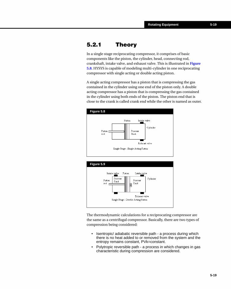
Rotating Equipment 5-19
5.2.1 TheoryIn a single stage reciprocating compressor, it comprises of basic components like the piston, the cylinder, head, connecting rod, crankshaft, intake valve, and exhaust valve. This is illustrated in Figure 5.8. HYSYS is capable of modeling multi-cylinder in one reciprocating compressor with single acting or double acting piston.
A single acting compressor has a piston that is compressing the gas contained in the cylinder using one end of the piston only. A double acting compressor has a piston that is compressing the gas contained in the cylinder using both ends of the piston. The piston end that is close to the crank is called crank end while the other is named as outer.
The thermodynamic calculations for a reciprocating compressor are the same as a centrifugal compressor. Basically, there are two types of compression being considered:
• Isentropic/ adiabatic reversible path - a process during which there is no heat added to or removed from the system and the entropy remains constant, PVk=constant.
• Polytropic reversible path - a process in which changes in gas characteristic during compression are considered.
Figure 5.8
Figure 5.9
5-19
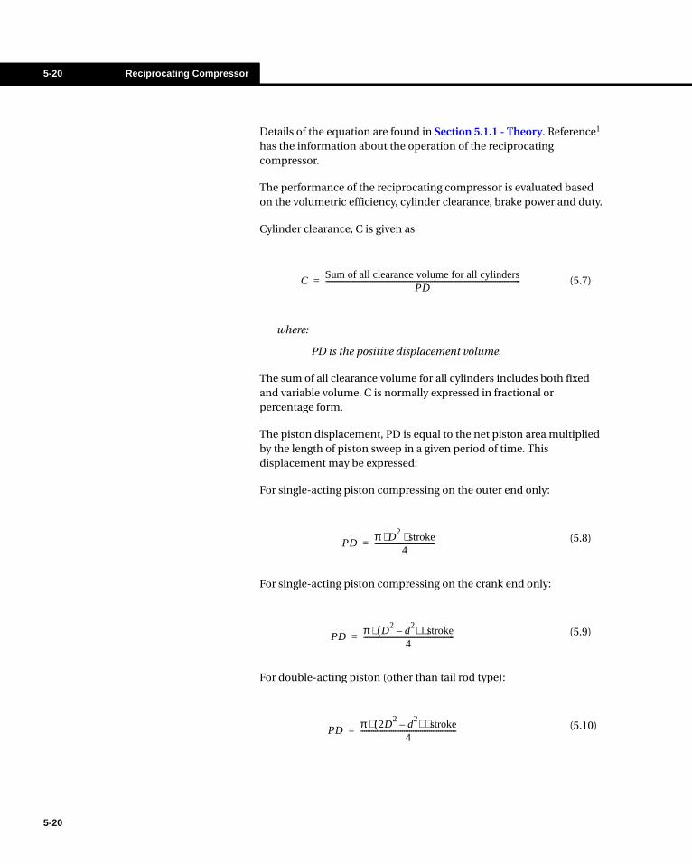
5-20 Reciprocating Compressor
5-20
Details of the equation are found in Section 5.1.1 - Theory. Reference1 has the information about the operation of the reciprocating compressor.
The performance of the reciprocating compressor is evaluated based on the volumetric efficiency, cylinder clearance, brake power and duty.
Cylinder clearance, C is given as
where:
PD is the positive displacement volume.
The sum of all clearance volume for all cylinders includes both fixed and variable volume. C is normally expressed in fractional or percentage form.
The piston displacement, PD is equal to the net piston area multiplied by the length of piston sweep in a given period of time. This displacement may be expressed:
For single-acting piston compressing on the outer end only:
For single-acting piston compressing on the crank end only:
For double-acting piston (other than tail rod type):
(5.7)CSum of all clearance volume for all cylinders
PD------------------------------------------------------------------------------------------------------------=
(5.8)PDπ D
2stroke⋅ ⋅
4---------------------------------=
(5.9)PDπ D
2d
2–( ) stroke⋅ ⋅
4--------------------------------------------------=
(5.10)PDπ 2D
2d
2–( ) stroke⋅ ⋅
4-----------------------------------------------------=

Rotating Equipment 5-21
For double-acting piston (tail rod type):
where:
d - piston rod diameter
D - piston diameter
PD includes the contributions from ALL cylinders and both ends of any double acting. If a cylinder is unloaded then its contribution does not factor in.
The volumetric efficiency is one of the important parameters used to evaluate the reciprocating compressor’s performance. Volumetric efficiency, VE, is defined as the actual pumping capacity of a cylinder compared to the piston displacement volume. VE is given by:
where:
Pd - Discharge pressure.
Ps - Suction pressure.
L - the effects of variable such as internal leakage, gas friction, pressure drop through valves and inlet gas preheating
k - Heat capacity ratio, Cp/Cv.
Zd - Discharge compressibility factor.
Zs - Suction compressibility factor.
C - Clearance volume
To account for losses at the suction and discharge valve, an arbitrary value about 4% VE loss is acceptable. For a non-lubricated compressor, an additional 5% loss is required to account for slippage of gas. If the compressor is in propane, or similar heavy gas service, an additional 4% should be subtracted from the volumetric efficiency. These
(5.11)PDπ 2D
22d
2–( ) stroke⋅ ⋅
4---------------------------------------------------------=
(5.12)VE 1 L–( ) CZs
Zd-----
Pd
Ps------
1k---
1––=
5-21
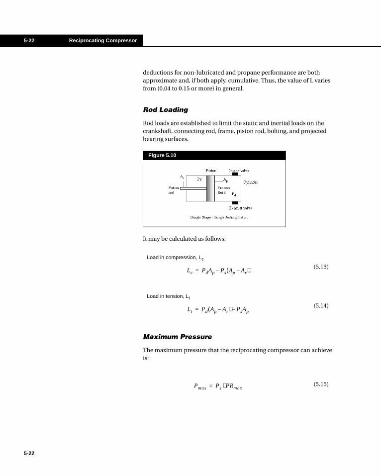
5-22 Reciprocating Compressor
5-22
deductions for non-lubricated and propane performance are both approximate and, if both apply, cumulative. Thus, the value of L varies from (0.04 to 0.15 or more) in general.
Rod Loading
Rod loads are established to limit the static and inertial loads on the crankshaft, connecting rod, frame, piston rod, bolting, and projected bearing surfaces.
It may be calculated as follows:
Maximum Pressure
The maximum pressure that the reciprocating compressor can achieve is:
Figure 5.10
Load in compression, Lc
(5.13)
Load in tension, Lt
(5.14)
Lc PdAp Ps Ap Ar–( )–=
Lt Pd Ap Ar–( ) PsAp–=
(5.15)Pmax Ps PRmax⋅=

Rotating Equipment 5-23
where the maximum discharge pressure ratio, PRmax is calculated from:
5.2.2 Design Tab
Connections Page
The Connections page is identical to the centrifugal compressor as shown in Figure 5.1. You must supply the names of the Inlet, Outlet and Energy Streams.
Parameters Page
The Parameters pages is identical to the centrifugal compressor as shown in Figure 5.2. You may specify the duty of the attached energy stream on this page, or allow HYSYS to calculate it. The adiabatic and polytropic efficiencies are displayed as well.
Note that you may specify only one efficiency, either adiabatic or polytropic. If you specify one efficiency and a solution is obtained, HYSYS will then back calculate the other efficiency, using the calculated duty and stream conditions. The reciprocating compressor has a higher adiabatic efficiency than the centrifugal type, normally in the range of 85% - 95%.
Links Page
The Links page is identical to the centrifugal compressor as shown in Figure 5.3.
(5.16)PRmax
Zd
Zs C⋅------------- 1 L– VE– C+( )
k=
5-23
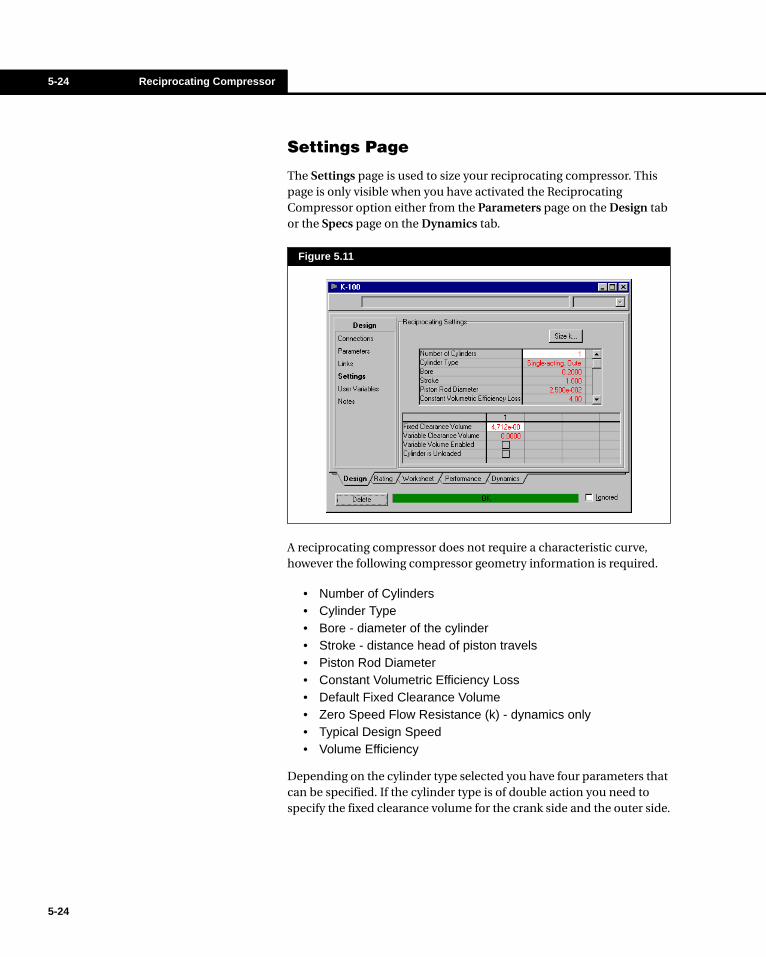
5-24 Reciprocating Compressor
5-24
Settings Page
The Settings page is used to size your reciprocating compressor. This page is only visible when you have activated the Reciprocating Compressor option either from the Parameters page on the Design tab or the Specs page on the Dynamics tab.
A reciprocating compressor does not require a characteristic curve, however the following compressor geometry information is required.
• Number of Cylinders• Cylinder Type• Bore - diameter of the cylinder• Stroke - distance head of piston travels• Piston Rod Diameter• Constant Volumetric Efficiency Loss• Default Fixed Clearance Volume• Zero Speed Flow Resistance (k) - dynamics only• Typical Design Speed• Volume Efficiency
Depending on the cylinder type selected you have four parameters that can be specified. If the cylinder type is of double action you need to specify the fixed clearance volume for the crank side and the outer side.
Figure 5.11

Rotating Equipment 5-25
• Fixed Clearance Volume• Variable Clearance Volume• Variable Volume Enabled• Cylinder is Unloaded - dynamics only
If the Variable Volume Enabled checkbox is checked you need to specify a Variable Clearance Volume. The variable volume is used when additional clearance volume (external) is intentionally added to reduce cylinder capacity.
If the Cylinder is Unloaded checkbox is checked the total displacement volume is not considered, and is essentially zero.
The Size k button is for dynamic use only, refer to the Dynamic Modelling Guide for more information.
User Variables Page
The User Variables page allows the user to create and implement variables in the HYSYS simulation case. For more information on implementing the User Variables option, see the User Variables chapter in the Customization Guide.
Notes Page
The Notes page provides a text editor where you can record any comments or information regarding the Compressor, or pertaining to your simulation in general.
5.2.3 Rating TabThe Rating tab contains two pages: Nozzles and Inertia page.
Nozzle Page
If you are working exclusively in Steady State mode, you are not required to change any information on the pages accessible through this page. For more information on running the Compressor operation in Dynamic mode, see the Dynamic Modeling guide for further details.
5-25
5-26 Reciprocating Compressor
5-26
Inertia Page
If you are working exclusively in Steady State mode, you are not required to change any information on this page. For more information on running the Compressor operation in Dynamic mode, see the Dynamic Modeling guide for further details.
5.2.4 Worksheet TabThe Worksheet tab contains a summary of the information contained in the stream property view for all the streams attached to the unit operation. The Conditions, Properties, and Composition pages contain selected information from the corresponding pages of the Worksheet tab for the stream property view. The PF Specs page contains a summary of the stream property view Dynamics tab.
5.2.5 Performance Tab
Results Page
On the Results page, you can view a table of calculated values for the Compressor.
• Adiabatic Head• Polytropic Head• Adiabatic Efficiency• Polytropic Efficiency• Duty• Polytropic Head Factor• Polytropic Exponent• Isentropic Exponent• Speed• Duty Loss• Total Effective Piston Displacement Volume• Total Effective Fractional Clearance Volume• Maximum Pressure Ratio• Lead in Compression• Load in Tension
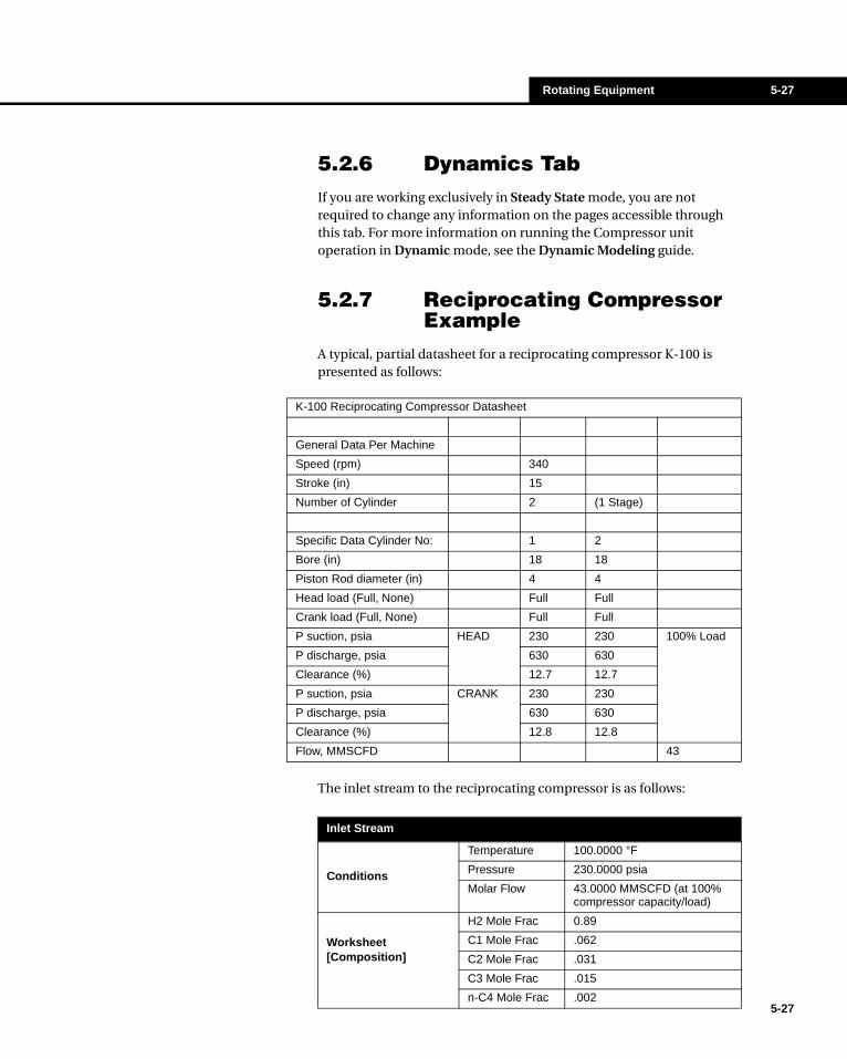
Rotating Equipment 5-27
5-27
5.2.6 Dynamics TabIf you are working exclusively in Steady State mode, you are not required to change any information on the pages accessible through this tab. For more information on running the Compressor unit operation in Dynamic mode, see the Dynamic Modeling guide.
5.2.7 Reciprocating Compressor Example
A typical, partial datasheet for a reciprocating compressor K-100 is presented as follows:
The inlet stream to the reciprocating compressor is as follows:
K-100 Reciprocating Compressor Datasheet
General Data Per Machine
Speed (rpm) 340
Stroke (in) 15
Number of Cylinder 2 (1 Stage)
Specific Data Cylinder No: 1 2
Bore (in) 18 18
Piston Rod diameter (in) 4 4
Head load (Full, None) Full Full
Crank load (Full, None) Full Full
P suction, psia HEAD 230 230 100% Load
P discharge, psia 630 630
Clearance (%) 12.7 12.7
P suction, psia CRANK 230 230
P discharge, psia 630 630
Clearance (%) 12.8 12.8
Flow, MMSCFD 43
Inlet Stream
Conditions
Temperature 100.0000 °F
Pressure 230.0000 psia
Molar Flow 43.0000 MMSCFD (at 100% compressor capacity/load)
Worksheet [Composition]
H2 Mole Frac 0.89
C1 Mole Frac .062
C2 Mole Frac .031
C3 Mole Frac .015
n-C4 Mole Frac .002

5-28 Reciprocating Compressor
5-28
It is required to increase the pressure of the feed gas to 630 psia. This compressor can be modeled according to the following steps.
1. Create a fluid package using the Peng Robinson property package and add the following components: H2, C1, C2, C3, and n-C4.
2. Install the stream Feed and define it as follows:
3. Install a Compressor unit operation with the following information:
4. To toggle the centrifugal compressor to a reciprocating compressor, activate the Reciprocating (Positive Displacement) check box found on the Dynamics tab.
5. On the Parameters page of the Design tab, toggle the centrifugal compressor to a reciprocating compressor by selecting the Reciprocating radio button. Also delete the default Adiabatic Efficiency value and specify the polytropic efficiency as 90.
Property Package Components
Peng Robinson H2, C1, C2, C3, n-C4
MATERIAL STREAM [Feed]
Tab [Page] Input Area Entry
Worksheet [Conditions]
Temperature 100.0000 °F
Pressure 230.0000 psia
Molar Flow 43.0000 MMSCFD (at 100% compressor capacity/load)
Worksheet [Composition]
H2 Mole Frac 0.89
C1 Mole Frac .062
C2 Mole Frac .031
C3 Mole Frac .015
n-C4 Mole Frac .002
Compressor [K-100]
Tab [Page] Input Area Entry
Design [Connections]
Inlet Feed
Outlet Out
Energy Comp Duty
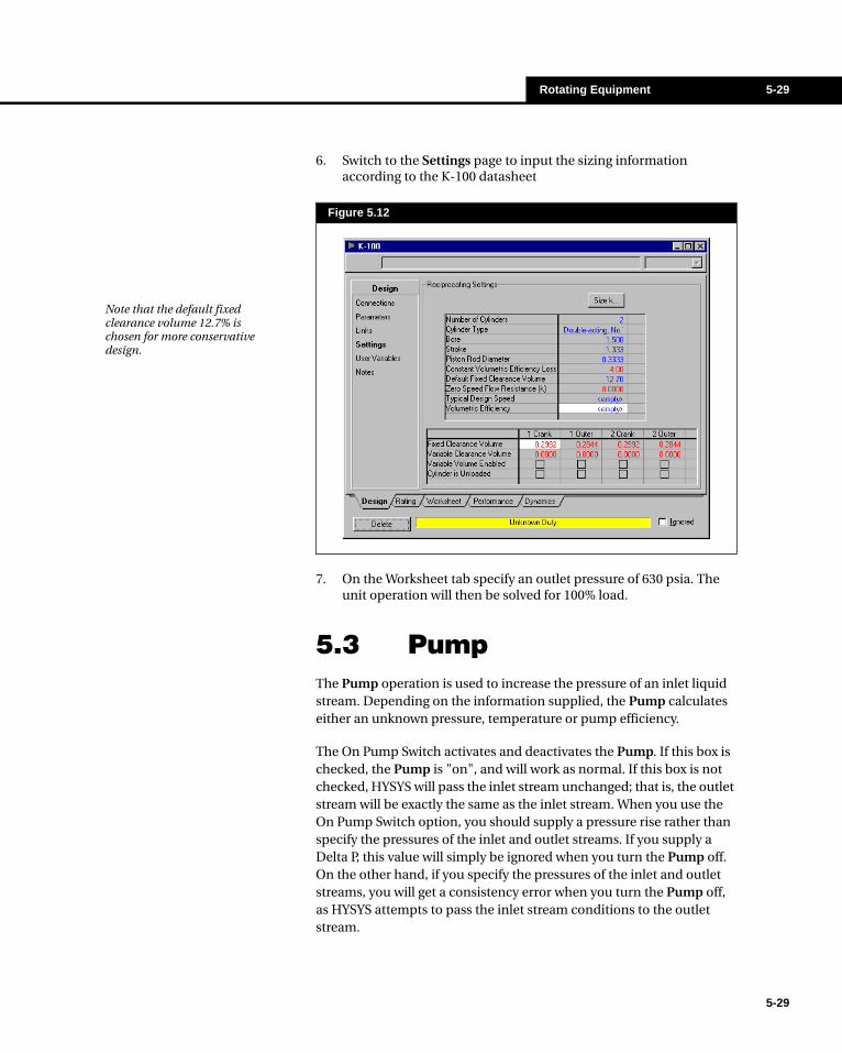
Rotating Equipment 5-29
6. Switch to the Settings page to input the sizing information according to the K-100 datasheet
7. On the Worksheet tab specify an outlet pressure of 630 psia. The unit operation will then be solved for 100% load.
5.3 PumpThe Pump operation is used to increase the pressure of an inlet liquid stream. Depending on the information supplied, the Pump calculates either an unknown pressure, temperature or pump efficiency.
The On Pump Switch activates and deactivates the Pump. If this box is checked, the Pump is "on", and will work as normal. If this box is not checked, HYSYS will pass the inlet stream unchanged; that is, the outlet stream will be exactly the same as the inlet stream. When you use the On Pump Switch option, you should supply a pressure rise rather than specify the pressures of the inlet and outlet streams. If you supply a Delta P, this value will simply be ignored when you turn the Pump off. On the other hand, if you specify the pressures of the inlet and outlet streams, you will get a consistency error when you turn the Pump off, as HYSYS attempts to pass the inlet stream conditions to the outlet stream.
Figure 5.12
Note that the default fixed clearance volume 12.7% is chosen for more conservative design.
5-29

5-30 Pump
5-30
To install the Pump operation, press F12 and choose Pump from the Unit Ops view or select the Pump button in the Object Palette.
To ignore the Pump during calculations, select the Ignore check box. HYSYS will completely disregard the operation (and will not calculate the outlet stream) until you restore it to an active state by clearing the check box.
5.3.1 TheoryCalculations are based on the standard pump equation for power, which uses the pressure rise, the liquid flow rate and density:
where: Pout = Pump outlet pressure
Pin = Pump inlet pressure
Note that the above equation defines the ideal power needed to raise the liquid pressure. The actual power requirement of the Pump is defined in terms of the Pump Efficiency:
When the efficiency is less than 100%, the excess energy goes into raising the temperature of the outlet stream.
Combining the above equations leads to the following expression for the actual power requirement of the Pump:
Finally, the actual power is equal to the difference in heat flow between the outlet and inlet streams:
Pump Button
(5.17)Power Requiredideal
Pout Pin–( ) Flow Rate×Liquid Density
---------------------------------------------------------------=
(5.18)Efficiency %( )Power Requiredideal
Power Requiredactual--------------------------------------------------------- 100%×=
(5.19)Power Requiredactual
Pout Pin–( ) Flow Rate 100%××Liquid Density Efficiency %( )×-----------------------------------------------------------------------------------=
Power Requiredactual = (Heat Flowoutlet - Heat Flowinlet) (5.20)

Rotating Equipment 5-31
If the feed is fully defined, only two of the following variables need to be supplied for the Pump to calculate all unknowns:
• Outlet Pressure or Pressure Drop• Efficiency• Pump Energy
HYSYS can also back-calculate the inlet Pressure.
If you choose to represent a pump by installing a Compressor in HYSYS, the power requirement and temperature rise of the Compressor will always be greater than those of the Pump (for the same fluid stream), because the Compressor treats the liquid as a compressible fluid. When the pressure of a compressible fluid increases, the temperature also increases, and the specific volume decreases. More work is required to move the fluid than if it were incompressible, exhibiting little temperature rise, as is the case with a HYSYS Pump.
Note that for a Pump, an efficiency of 100% does not correspond to a true isentropic compression of the liquid. Pump calculations are performed by HYSYS with the assumption that the liquid is incompressible; that is, the density is constant (liquid volume is independent of pressure). This is the usual assumption for liquids well removed from the critical point, and the standard pump equation given above is generally accepted for calculating the power requirement. However, if you wish to perform a more rigorous calculation for pumping a compressible liquid (i.e. one near the critical point), you should instead install a Compressor to represent the Pump.
5-31
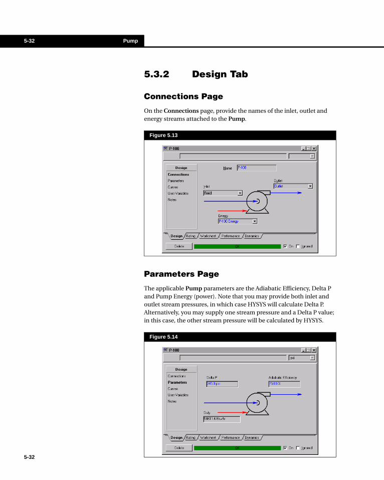
5-32 Pump
5-32
5.3.2 Design Tab
Connections Page
On the Connections page, provide the names of the inlet, outlet and energy streams attached to the Pump.
Parameters Page
The applicable Pump parameters are the Adiabatic Efficiency, Delta P and Pump Energy (power). Note that you may provide both inlet and outlet stream pressures, in which case HYSYS will calculate Delta P. Alternatively, you may supply one stream pressure and a Delta P value; in this case, the other stream pressure will be calculated by HYSYS.
Figure 5.13
Figure 5.14
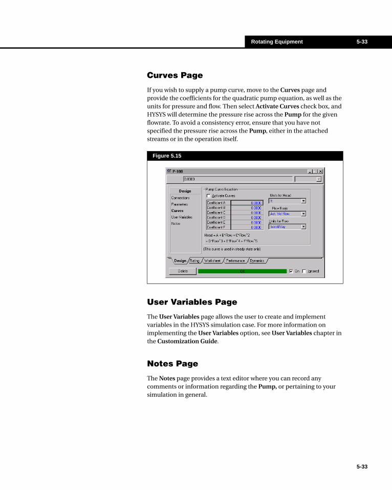
Rotating Equipment 5-33
Curves Page
If you wish to supply a pump curve, move to the Curves page and provide the coefficients for the quadratic pump equation, as well as the units for pressure and flow. Then select Activate Curves check box, and HYSYS will determine the pressure rise across the Pump for the given flowrate. To avoid a consistency error, ensure that you have not specified the pressure rise across the Pump, either in the attached streams or in the operation itself.
User Variables Page
The User Variables page allows the user to create and implement variables in the HYSYS simulation case. For more information on implementing the User Variables option, see User Variables chapter in the Customization Guide.
Notes Page
The Notes page provides a text editor where you can record any comments or information regarding the Pump, or pertaining to your simulation in general.
Figure 5.15
5-33

5-34 Pump
5-34
5.3.3 Rating TabIf you are working exclusively in Steady State mode, you are not required to change any information on the pages accessible through this tab. For more information on running the Pump unit operation in Dynamic mode, see the Dynamic Modeling guide.
5.3.4 Worksheet TabThe Worksheet tab contains a summary of the information contained in the stream property view for all the streams attached to the unit operation. The Conditions, Properties, and Composition pages contain selected information from the corresponding pages of the Worksheet tab for the stream property view. The PF Specs page contains a summary of the stream property view Dynamics tab.
5.3.5 Performance Tab
Results Page
The Results page contains pump head information. The values for Pressure Head, Velocity Head and Delta P excluding static head are calculated values.
The Total Head cell is used only for Dynamic simulation. For more information regarding this please refer to Chapter 6 - Rotating Equipment of the Dynamic Modeling guide.
5.3.6 Dynamics TabThe Dynamics tab is used only for Dynamic simulation. For more information regarding this tab, please refer to Chapter 6 - Rotating Equipment of the Dynamic Modeling guide.

Rotating Equipment 5-35
5.3.7 Pump ExampleTo illustrate the use of the Pump Operation, stream FEED will be pumped from 455 psia to 800 psia. The pump efficiency is 75 percent.
1. Create a fluid package using the Peng Robinson EOS and the following components: C1, C2, C3, i-C4, n-C4, i-C5, n-C5, n-C6, n-C7, n-C8.
2. Create a stream named Feed and define it as follows:
3. Now install the Pump unit operation and provide the following information:
Property Package Components
Peng Robinson C1, C2, C3, i-C4, n-C4, i-C5, n-C5, n-C6, n-C7, n-C8
MATERIAL STREAM [Feed]
Tab [Page] Input Area Entry
Worksheet [Conditions]
Temperature 250.0000 °F
Pressure 455.0000 psi
Molar Flow 300.0000 lbmole/hr
Worksheet [Composition]
Methane Mole Frac 0.0000
Ethane Mole Frac 0.0001
Propane Mole Frac 0.0200
i-Butane Mole Frac 0.1859
n-Butane Mole Frac 0.1748
i-Pentane Mole Frac 0.1592
n-Pentane Mole Frac 0.1372
n-Hexane Mole Frac 0.1613
n-Heptane Mole Frac 0.0923
n-Octane Mole Frac 0.0692
Pump [P-100]
Tab [Page] Input Area Entry
Design [Connections]
Inlet Feed
Outlet Outlet
Energy P-100 Energy
Design [Parameters]Adiabatic Efficiency 75%
Delta P 345 psi
5-35
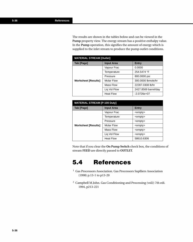
5-36 References
5-36
The results are shown in the tables below and can be viewed in the Pump property view. The energy stream has a positive enthalpy value. In the Pump operation, this signifies the amount of energy which is supplied to the inlet stream to produce the pump outlet conditions.
Note that if you clear the On Pump Switch check box, the conditions of stream FEED are directly passed to OUTLET.
5.4 References 1 Gas Processors Association. Gas Processors Suplliers Association
(1998) p.13-1 to p13-20
2 Campbell M.John. Gas Conditioning and Processing (vol2) 7th edi. 1994, p213-221
MATERIAL STREAM [Outlet]
Tab [Page] Input Area Entry
Worksheet [Results]
Vapour Frac 0.0000
Temperature 254.5474 °F
Pressure 800.0000 psi
Molar Flow 300.0000 lbmole/hr
Mass Flow 22287.0308 lb/hr
Liq Vol Flow 2427.8569 barrel/day
Heat Flow -2.0726e+07
MATERIAL STREAM [P-100 Duty]
Tab [Page] Input Area Entry
Worksheet [Results]
Vapour Frac <empty>
Temperature <empty>
Pressure <empty>
Molar Flow <empty>
Mass Flow <empty>
Liq Vol Flow <empty>
Heat Flow 58610.6306

Separation Operations 6-1
6 Separation Operations
6-1
6.1 Separator / 3-Phase Separator / Tank......................................................... 3
6.1.1 Theory...................................................................................................... 36.1.2 Design Tab ............................................................................................... 56.1.3 Reactions Tab .......................................................................................... 76.1.4 Rating Tab................................................................................................ 86.1.5 Worksheet Tab ......................................................................................... 96.1.6 Dynamics Tab .......................................................................................... 96.1.7 3-Phase Separation Example .................................................................. 9
6.2 Shortcut Column ........................................................................................ 11
6.2.1 Design Tab ..............................................................................................116.2.2 Rating Tab.............................................................................................. 136.2.3 Worksheet Tab ....................................................................................... 136.2.4 Performance Tab.................................................................................... 136.2.5 Dynamics Tab ........................................................................................ 146.2.6 Shortcut Column Example ..................................................................... 14
6.3 Component Splitter .................................................................................... 16
6.3.1 Theory.................................................................................................... 176.3.2 Design Tab ............................................................................................. 186.3.3 Rating Tab.............................................................................................. 206.3.4 Worksheet .............................................................................................. 206.3.5 Dynamics Tab ........................................................................................ 206.3.6 Example ................................................................................................. 20

6-2
6-2

Separation Operations 6-3
6.1 Separator / 3-Phase Separator / Tank
Because the property views for SEPARATOR, 3-PHASE SEPARATOR and TANK are almost identical, these three unit operations are discussed together in this section. There is an Operation Toggle on the Parameters page of the Design tab that allows you to easily switch from one of these operations to another. For example, you may wish to change a fully defined SEPARATOR to a 3-PHASE SEPARATOR. Simply select the appropriate radio button using the operation toggle. The only additional information required would be to identify the additional liquid stream. All of the original characteristics of the operation (Parameters, Reactions, etc.) will be retained. The key differences in these operations are the stream connections (related to the feed separation):
6.1.1 TheoryA P-H flash is performed to determine the product conditions and phases. The pressure at which the flash is performed is the lowest feed pressure minus the pressure drop across the vessel. The enthalpy is the combined feed enthalpy plus or minus the duty (for heating, the duty is added; for cooling, the duty is subtracted).
As well as standard forward applications, the SEPARATOR and 3-PHASE SEPARATOR have the ability to back-calculate results. In addition to the standard application (completely defined feed stream(s) being separated at the vessel pressure and enthalpy), the SEPARATOR can also use a known product composition to determine the composition(s) of the other product stream(s), and by a balance the feed composition.
All information in this section applies to the SEPARATOR, the 3-PHASE SEPARATOR and the TANK Operation, unless indicated otherwise.
Operation Description
Separator
Multiple feeds, one vapour and one liquid product stream. In Steady-State mode, the SEPARATOR divides the vessel contents into its constituent vapour and liquid phases.
3-Phase Separator
Multiple feeds, one vapour and two liquid product streams. The 3-PHASE SEPARATOR operation divides the vessel contents into its constituent vapour, light liquid and heavy liquid phases.
TankMultiple feeds, and one liquid product stream. The TANK is generally used to simulate liquid surge vessels.
Separator Button
3-Phase Separator Button
Tank Button
For a detailed explanation of Separator Dynamics, see Chapter 7 - Separation Operations in the Dynamic Modeling Guide.
6-3
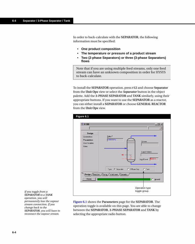
6-4 Separator / 3-Phase Separator / Tank
6-4
In order to back-calculate with the SEPARATOR, the following information must be specified:
• One product composition• The temperature or pressure of a product stream• Two (2-phase Separators) or three (3-phase Separators)
flows
To install the SEPARATOR operation, press F12 and choose Separator from the Unit Ops view or select the Separator button in the object palette. Add the 3-PHASE SEPARATOR and TANK similarly, using their appropriate buttons. If you want to use the SEPARATOR as a reactor, you can either install a SEPARATOR or choose GENERAL REACTOR from the Unit Ops view.
Figure 6.1 shows the Parameters page for the SEPARATOR. The operation toggle is available on this page. You are able to change between the SEPARATOR, 3-PHASE SEPARATOR and TANK by selecting the appropriate radio button.
Figure 6.1
Note that if you are using multiple feed streams, only one feed stream can have an unknown composition in order for HYSYS to back-calculate.
Operation type toggle group.If you toggle from a
SEPARATOR to a TANK operation, you will permanently lose the vapour stream connection. If you change back to the SEPARATOR, you will have to reconnect the vapour stream.
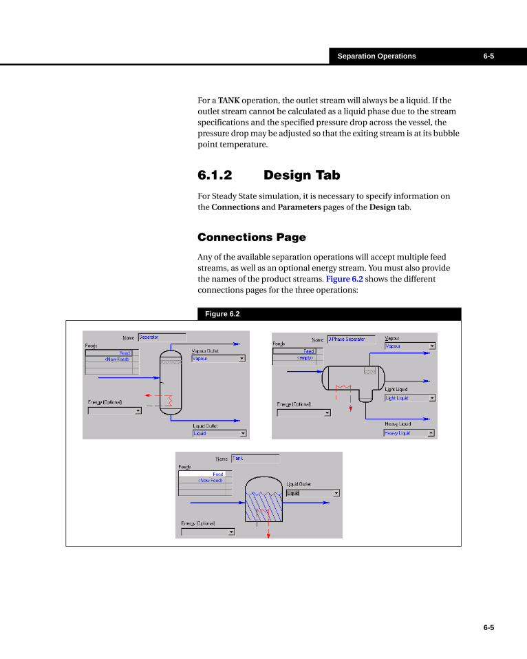
Separation Operations 6-5
For a TANK operation, the outlet stream will always be a liquid. If the outlet stream cannot be calculated as a liquid phase due to the stream specifications and the specified pressure drop across the vessel, the pressure drop may be adjusted so that the exiting stream is at its bubble point temperature.
6.1.2 Design TabFor Steady State simulation, it is necessary to specify information on the Connections and Parameters pages of the Design tab.
Connections Page
Any of the available separation operations will accept multiple feed streams, as well as an optional energy stream. You must also provide the names of the product streams. Figure 6.2 shows the different connections pages for the three operations:
Figure 6.2
6-5

6-6 Separator / 3-Phase Separator / Tank
6-6
Heat Transfer
You may also specify an energy input to the vessel by providing the name of the Energy stream on the Connections page. The Steady-State mode separator energy balance is defined below:
where: Hfeed = Heat flow of the feed stream(s)
Hvapour = Heat flow of the vapour product stream
Hlight = Heat flow of the light liquid product stream
Hheavy = Heat flow of the heavy liquid product stream
Parameters Page
The Parameters page allows you to specify the Pressure Drop across the vessel. The following Vessel Parameters are displayed:
Physical Parameters
The Physical Parameters associated with this operation are the Pressure Drop across the vessel (Delta P) and the Vessel Volume. The pressure drop is defined as:
where: P = Vessel pressure
Pv = Pressure of vapour product stream (not applicable for Tank)
Pl = Pressure of liquid product stream(s)
Pfeed = Pressure of feed stream
DP = Pressure drop in vessel (Delta P)
(6.1)Hfeed Duty± Hvapour Hheavy Hlight+ +=
Vessel Parameter Description
Vessel Volume This is a user-specified parameter.
Liquid Level SP Expressed as a percentage of the Full (Vessel) Volume. This is a user-specified parameter.
Liquid VolumeNot set by the user. The Liquid Volume is calculated from the product of the Vessel Volume and Liquid Level fraction.
P = Pv = Pl = Pfeed - DP (3.1)Note that Pfeed is assumed to be the lowest pressure of all the feed streams.
Separation Operations 6-7
The default pressure drop across the vessel is zero.
The Vessel Volume, together with the Set Point for liquid level/flow, defines the amount of holdup in the Vessel. The amount of liquid volume, or holdup, in the vessel at any time is given by the following expression
where: PV(%Full) is the liquid level in the vessel at time t.
The default vessel volume is 2 m3.
User Variables Page
On this page you can write User Variables associated with the operation to increase its functionality within your simulation case. For more information on creating and executing User Variables in HYSYS, see the User Variables chapter in the Customization Guide, available with the on-line documentation.
Notes Page
A text field is available on this page that lets you to write and store information and comments regarding the specific unit operation, or about your case in general.
6.1.3 Reactions Tab
Results Page
Reaction Sets may be attached to the SEPARATOR, 3-PHASE SEPARATOR, or TANK Operations. You may attach a Reaction Set to the operation by selecting it from the drop down list. The Set Status field will display the status (Ready or Not Ready) of the currently selected Reaction Set.
The Vessel Volume is necessary in Steady State when modeling a Reactor (CSTR), as it determines the residence time.
(6.2)Holdup Vessel VolumePV %Full( )
100-----------------------------×=
6-7
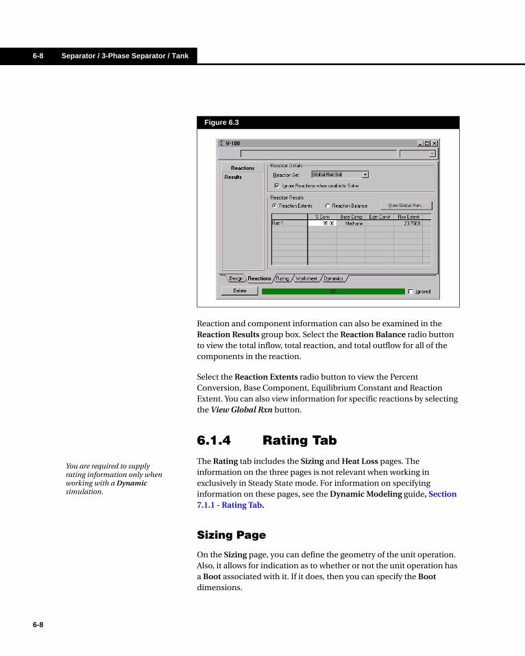
6-8 Separator / 3-Phase Separator / Tank
6-8
Reaction and component information can also be examined in the Reaction Results group box. Select the Reaction Balance radio button to view the total inflow, total reaction, and total outflow for all of the components in the reaction.
Select the Reaction Extents radio button to view the Percent Conversion, Base Component, Equilibrium Constant and Reaction Extent. You can also view information for specific reactions by selecting the View Global Rxn button.
6.1.4 Rating TabThe Rating tab includes the Sizing and Heat Loss pages. The information on the three pages is not relevant when working in exclusively in Steady State mode. For information on specifying information on these pages, see the Dynamic Modeling guide, Section 7.1.1 - Rating Tab.
Sizing Page
On the Sizing page, you can define the geometry of the unit operation. Also, it allows for indication as to whether or not the unit operation has a Boot associated with it. If it does, then you can specify the Boot dimensions.
Figure 6.3
You are required to supply rating information only when working with a Dynamic simulation.

Separation Operations 6-9
Heat Loss Page
The Heat Loss page allows you to specify which Heat Loss Model you want to implement and to define the parameters associated with each model.
6.1.5 Worksheet TabThe Worksheet tab contains a summary of the information available in the stream property view for all the streams attached to the unit operation. The Conditions, Properties, and Composition pages contain selected information from the corresponding pages of the Worksheet tab for the stream property view. The PF Specs page contains a summary of the stream property view Dynamics tab.
6.1.6 Dynamics TabInformation available on this page is relevant only to cases in Dynamics mode. For information on Dynamic simulation, see the HYSYS Dynamic Modeling Guide.
6.1.7 3-Phase Separation Example
A simple three-phase separation is illustrated in this example. Create a New HYSYS case with the following properties:
Create a stream named Feed with the following properties:
Property Package Components
Peng Robinson C1, C2, C3, i-C4, n-C4, i-C5, n-C5, H2O
New Case Button
MATERIAL STREAM [Feed]
Tab [Page] Input Area Entry
Worksheet [Conditions]
Temperature [C] 20.0000
Pressure [kPa] 200.0000
Molar Flow [kgmole/hr] 100.0000
6-9

6-10 Separator / 3-Phase Separator / Tank
6-10
Note that this stream has three phases. You can verify this by expanding the Worksheet tab of the Feed property view.
Install the 3-PHASE SEPARATOR. On the Connections page of the Design tab, input the information in the table below. For the remainder of the fields, the 3-PHASE SEPARATOR default values will be used.
These are the results that can be found on the Worksheet tab:
Worksheet [Composition]
Methane Mole Frac 0.1000
Ethane Mole Frac 0.0300
Propane Mole Frac 0.0400
i-Butane Mole Frac 0.0800
n-Butane Mole Frac 0.1000
i-Pentane Mole Frac 0.1200
n-Pentane Mole Frac 0.1300
H2O Mole Frac 0.4000
MATERIAL STREAM [Feed]
Tab [Page] Input Area Entry
3-Phase Separator Button
3-PHASE SEPARATOR [3-Phase Separator]
Tab [Page] Input Area Entry
Design [Connections]
Feeds Feed
Vapour Vapour
Light Liquid Light
Heavy Liquid Heavy
Figure 6.4

Separation Operations 6-11
6.2 Shortcut ColumnThe SHORTCUT COLUMN performs Fenske-Underwood short cut calculations for simple refluxed towers. The Fenske minimum number of trays and the Underwood minimum reflux are calculated. A specified reflux ratio can then be used to calculate the vapour and liquid traffic rates in the enriching and stripping sections, the condenser duty and reboiler duty, the number of ideal trays, and the optimal feed location.
The SHORTCUT COLUMN is only an estimate of the column performance and is restricted to simple refluxed columns. For more realistic results the rigorous COLUMN operation should be used. This operation can provide initial estimates for most simple columns.
To install the SHORTCUT COLUMN operation, press F12 and choose Shortcut Column from the Unit Ops view or select the Shortcut Column button in the Object Palette.
6.2.1 Design Tab
Connections Page
The Connections page of the Design tab of the SHORTCUT COLUMN is shown in Figure 6.5. A feed stream, overhead product, bottoms product, condenser and reboiler duty name should all be specified. The overhead product can either be an Overhead Vapour or a Distillate stream, depending on the radio button selection in the Top Product Phase group. The operation name can also be changed on this page.
Figure 6.5
Shortcut Column Button
You can specify the top product to be either liquid or vapour using the radio buttons in the Top Product Phase group.
6-11

6-12 Shortcut Column
6-12
Parameters Page
The SHORTCUT COLUMN requires the light and heavy key components (keys) to be defined. The light key is the more volatile component of the two main components that are to be separated. The compositions of the keys are used to specify the distillation products. The composition of the light key in the bottoms and the heavy key in the overhead are the only composition specifications required.
In the Components group, select a Light Key and Heavy Key from the drop down list in the Edit Bar and supply their corresponding mole fraction specifications. The specification must be such that there is enough of both keys to be distributed in the bottoms and overhead. It is possible to specify a large value for the light key composition such that too much of the light key is in the bottoms and the overhead heavy key composition spec cannot be met. If this problem occurs, one or both of the key specs must be changed.
Define the column pressure profile by specifying a Condenser Pressure and a Reboiler Pressure in the Pressures group.
In the Reflux Ratios group, the calculated Minimum Reflux Ratio will be displayed once streams are attached on the Connections page and the required parameters are specified in the Components and Pressures groups.
Figure 6.6
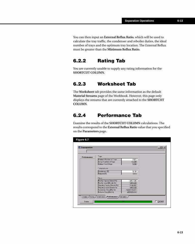
Separation Operations 6-13
You can then input an External Reflux Ratio, which will be used to calculate the tray traffic, the condenser and reboiler duties, the ideal number of trays and the optimum tray location. The External Reflux must be greater than the Minimum Reflux Ratio.
6.2.2 Rating TabYou are currently unable to supply any rating information for the SHORTCUT COLUMN.
6.2.3 Worksheet TabThe Worksheet tab provides the same information as the default Material Streams page of the Workbook. However, this page only displays the streams that are currently attached to the SHORTCUT COLUMN.
6.2.4 Performance TabExamine the results of the SHORTCUT COLUMN calculations. The results correspond to the External Reflux Ratio value that you specified on the Parameters page.
Figure 6.7
6-13

6-14 Shortcut Column
6-14
The following results are available:
6.2.5 Dynamics TabThe SHORTCUT COLUMN currently runs only in Steady State mode. As such, there is no information available on the Dynamics tab.
6.2.6 Shortcut Column ExampleThe following example builds a SHORTCUT COLUMN as a typical depropanizer, having the stream Feed as the tower feed. Start building the case with the following properties:
Create the stream Feed with the following properties:.
Column Result Description
Minimum Number of TraysThis is the Fenske minimum number of trays, which is not affected by the External Reflux Ratio specification.
Actual Number of Trays This is calculated using a using the Gilliland method.
Optimal Feed Stage Top down feed stage for optimal separation.
Condenser and Reboiler Temperatures
These temperatures are not affected by the External Reflux Ratio specification.
Rectifying Section Vapour and Liquid traffic flow rates
These are the estimated average flow rates above the feed location.
Stripping Section Vapour and Liquid traffic flow rates
These are the estimated average flow rates below the feed location.
Condenser and Reboiler Duties The duties, as calculated by HYSYS.
Property Package Components
Peng Robinson C2, C3, i-C4, n-C4, i-C5, n-C5, C6
MATERIAL STREAM [Feed]
Tab [Page] Input Area Entry
Worksheet [Conditions]
Temperature [F] 207.37
Pressure [psia] 100.0000
Molar Flow [lbmole/hr] 1271.5190
Separation Operations 6-15
Install a SHORTCUT COLUMN to your case. On the Connections page of the Design tab, complete the fields as follows:
Supply the following information on the Parameters page of the Design tab:
HYSYS will automatically calculate the Minimum Reflux Ratio as 0.979.
Worksheet [Composition]
Ethane Mole Frac 0.0148
Propane Mole Frac 0.7315
i-Butane Mole Frac 0.0681
n-Butane Mole Frac 0.1462
i-Pentane Mole Frac 0.0173
n-Pentane Mole Frac 0.0150
n-Hexane Mole Frac 0.0071
MATERIAL STREAM [Feed]
Tab [Page] Input Area Entry
Shortcut Column ButtonSHORTCUT COLUMN [Depropanizer]
Tab [Page] Input Area Entry
Design [Connections]
Feed Feed
Distillate Distillate
Bottoms Bottoms
Condenser Duty Cond Q
Reboiler Duty Reb Q
Top Product Phase Liquid
SHORTCUT COLUMN [Depropanizer]
Tab [Page] Input Area Entry
Design [Parameters]
Light Key in Bottom Component - Propane
Mole Fraction - 0.025
Heavy Key in Distillate
Component - i-Butane
Mole Fraction - 0.020
Condenser Pressure 100 psia
Reboiler Pressure 103 psia
External Reflux Ratio 1.5
6-15
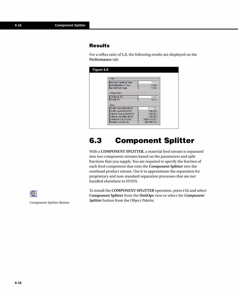
6-16 Component Splitter
6-16
Results
For a reflux ratio of 1.5, the following results are displayed on the Performance tab:
6.3 Component SplitterWith a COMPONENT SPLITTER, a material feed stream is separated into two component streams based on the parameters and split fractions that you supply. You are required to specify the fraction of each feed component that exits the Component Splitter into the overhead product stream. Use it to approximate the separation for proprietary and non-standard separation processes that are not handled elsewhere in HYSYS.
To install the COMPONENT SPLITTER operation, press F12 and select Component Splitter from the UnitOps view or select the Component Splitter button from the Object Palette.
Figure 6.8
Component Splitter Button

Separation Operations 6-17
6.3.1 TheoryThe Component Splitter satisfies the material balance for each component:
where: fi = Molar flow of the ith component in the feed
ai = Molar flow of the ith component in the overhead
bi = Molar flow in the ith component in the bottoms
The molar flows going to the overhead and bottoms are calculated as:
where: xi = Split, or fraction of component i going to the overhead
Once the composition, vapour fraction and pressure of the outlet streams are know, a P-VF flash is performed to obtain the temperatures and heat flows.
An overall heat balance is performed to obtain the energy stream heat flow:
where: hE = Enthalpy of unknown Energy Stream
hF = Enthalpy of Feed Stream
hO = Enthalpy of Overhead Stream
hB = Enthalpy of Bottoms Stream
fi = ai + bi (6.3)
ai = xi fi (6.4)
bi = (1-xi ) fi (6.5)
hE = hF - hO - hB (6.6)
6-17

6-18 Component Splitter
6-18
6.3.2 Design Tab
Connections Page
On the Connections page, you can specify an unlimited number of Feed streams to the Component Splitter. Overhead and Bottoms product streams must also be specified, and an unlimited number of Energy streams may be specified as well.
One of the attached energy streams should have an unspecified energy value to allow the operation to solve the energy balance.
Parameters Tab
This page displays the stream parameters that must be specified. Included are the vapour fraction and pressure of the Overhead and Bottoms streams.
Figure 6.9
Figure 6.10
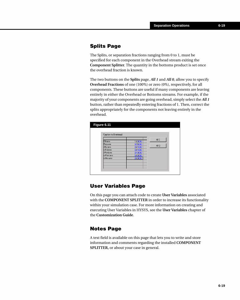
Separation Operations 6-19
Splits Page
The Splits, or separation fractions ranging from 0 to 1, must be specified for each component in the Overhead stream exiting the Component Splitter. The quantity in the bottoms product is set once the overhead fraction is known.
The two buttons on the Splits page, All 1 and All 0, allow you to specify Overhead Fractions of one (100%) or zero (0%), respectively, for all components. These buttons are useful if many components are leaving entirely in either the Overhead or Bottoms streams. For example, if the majority of your components are going overhead, simply select the All 1 button, rather than repeatedly entering fractions of 1. Then, correct the splits appropriately for the components not leaving entirely in the overhead.
User Variables Page
On this page you can attach code to create User Variables associated with the COMPONENT SPLITTER in order to increase its functionality within your simulation case. For more information on creating and executing User Variables in HYSYS, see the User Variables chapter of the Customization Guide.
Notes Page
A text field is available on this page that lets you to write and store information and comments regarding the installed COMPONENT SPLITTER, or about your case in general.
Figure 6.11
6-19

6-20 Component Splitter
6-20
6.3.3 Rating TabYou are not able to provide any information for the Component Splitter on the Rating tab when in Steady State. For information on Dynamic simulation, see the HYSYS Dynamic Modeling Guide.
6.3.4 WorksheetThe Worksheet tab provides the same information as the default Material Streams page of the Workbook. However, this page only displays the streams that are currently attached to the COMPONENT SPLITTER.
6.3.5 Dynamics TabInformation available on this page is relevant only to cases in Dynamics mode. For information on Dynamic simulation, see the HYSYS Dynamic Modeling Guide.
6.3.6 ExampleThe following example illustrates the use of the COMPONENT SPLITTER. Stream 1 is the attached feed stream; stream 2 is the overhead product stream, and stream 3 is the bottom product stream. The energy stream is Q-100.
Create a case with the following Fluid Package:
Define the feed stream 1 as follows:
Property Package Components
Peng-Robinson Ethane, Propane, i-Butane, n-Butane, i-Pentane, n-Pentane, n-Hexane
MATERIAL STREAM [1]
Tab [Page] Input Area Entry
Worksheet [Conditions]
Temperature [F] 200.0000
Pressure [psia] 500.0000
Molar Flow [lbmole/hr] 1000.0000

Separation Operations 6-21
Now install a COMPONENT SPLITTER. Complete the Connections page is shown in Figure 6.12:
Complete the Parameters page with the following information:
The splits for the Overhead stream are specified on the Splits page:
Worksheet [Composition]
Ethane Mole Frac 0.0148
Propane Mole Frac 0.7315
i-Butane Mole Frac 0.0681
n-Butane Mole Frac 0.1462
i-Pentane Mole Frac 0.0173
n-Pentane Mole Frac 0.0150
n-Hexane Mole Frac 0.0071
MATERIAL STREAM [1]
Tab [Page] Input Area Entry
Figure 6.12
Figure 6.13
Figure 6.14
Component Splitter Button
6-21
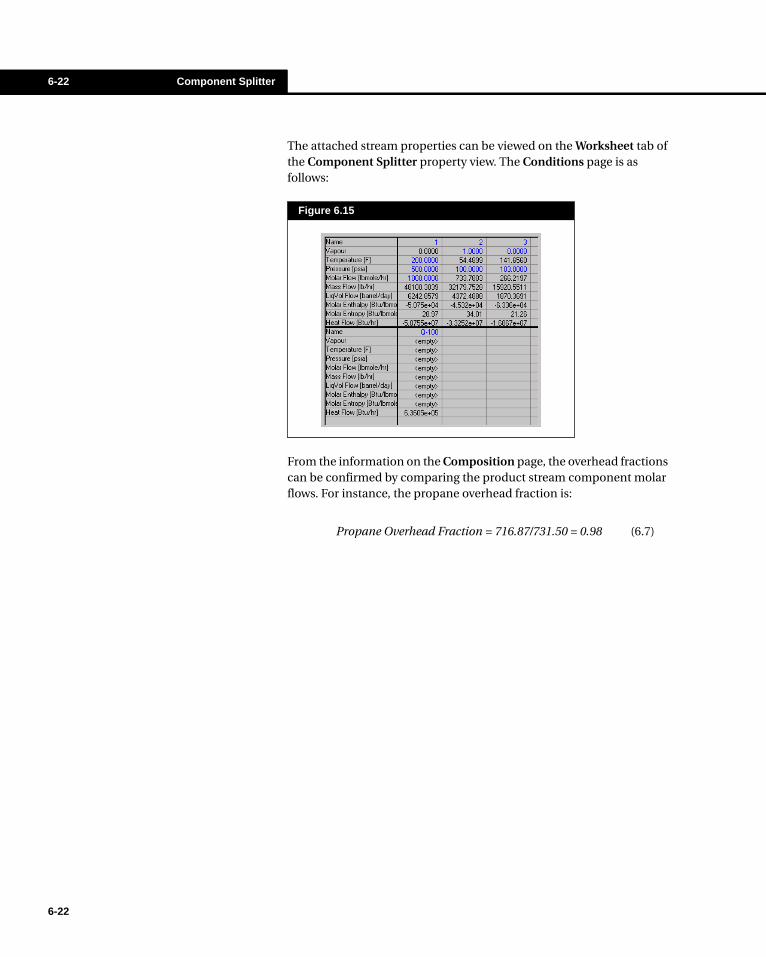
6-22 Component Splitter
6-22
The attached stream properties can be viewed on the Worksheet tab of the Component Splitter property view. The Conditions page is as follows:
From the information on the Composition page, the overhead fractions can be confirmed by comparing the product stream component molar flows. For instance, the propane overhead fraction is:
Figure 6.15
Propane Overhead Fraction = 716.87/731.50 = 0.98 (6.7)
Column 7-1
7 Column
7.1 Column Subflowsheet.................................................................................. 3
7.2 Column Theory ............................................................................................. 8
7.2.1 Three Phase Theory ................................................................................ 97.2.2 Detection of Three Phases .................................................................... 107.2.3 Initial Estimates...................................................................................... 10
7.3 Column Installation .................................................................................... 12
7.3.1 Input Experts .......................................................................................... 137.3.2 Templates............................................................................................... 14
7.4 Column Property View ............................................................................... 20
7.4.1 Design Tab ............................................................................................. 217.4.2 Parameters Tab...................................................................................... 337.4.3 Side Ops Tab ......................................................................................... 477.4.4 Rating Tab.............................................................................................. 517.4.5 Worksheet Tab ....................................................................................... 527.4.6 Performance Tab.................................................................................... 527.4.7 Flowsheet Tab........................................................................................ 607.4.8 Reactions Tab ........................................................................................ 637.4.9 Dynamics Tab ........................................................................................ 69
7.5 Column Specification Types ..................................................................... 69
7.5.1 Cold Property Specifications .................................................................. 707.5.2 Component Flow Rate ........................................................................... 707.5.3 Component Fractions............................................................................. 717.5.4 Component Ratio ................................................................................... 717.5.5 Component Recovery ............................................................................ 717.5.6 Cut Point ................................................................................................ 727.5.7 Draw Rate .............................................................................................. 727.5.8 Delta T (Heater/Cooler).......................................................................... 72
7-1

7-2
7-2
7.5.9 Delta T (Streams)................................................................................... 737.5.10 Duty...................................................................................................... 737.5.11 Duty Ratio............................................................................................. 737.5.12 Feed Ratio ........................................................................................... 737.5.13 Gap Cut Point ...................................................................................... 747.5.14 Liquid Flow........................................................................................... 747.5.15 Physical Property Specifications.......................................................... 747.5.16 Pump Around Specifications................................................................ 757.5.17 Reboil Ratio ......................................................................................... 757.5.18 Reflux Ratio ......................................................................................... 767.5.19 Tee Split Fraction ................................................................................. 767.5.20 Tray Temperature................................................................................. 767.5.21 Transport Property Specifications ........................................................ 777.5.22 User Property ....................................................................................... 777.5.23 Vapor Flow ........................................................................................... 777.5.24 Vapor Fraction...................................................................................... 787.5.25 Vapor Pressure Specifications ............................................................. 787.5.26 Column Stream Specifications............................................................. 78
7.6 Column-Specific Operations..................................................................... 79
7.6.1 Condenser ............................................................................................. 807.6.2 Reboiler.................................................................................................. 857.6.3 Tray Section ........................................................................................... 877.6.4 Tee ......................................................................................................... 92
7.7 Running the Column.................................................................................. 94
7.7.1 Run ........................................................................................................ 947.7.2 Reset...................................................................................................... 95
7.8 Column Troubleshooting........................................................................... 96
7.8.1 Heat and Spec Errors Fail to Converge ................................................. 967.8.2 Equilibrium Error Fails to Converge ..................................................... 1007.8.3 Equilibrium Error Oscillates.................................................................. 100
7.9 References................................................................................................ 100

Column 7-3
7.1 Column SubflowsheetThe Column is a special type of subflowsheet in HYSYS. A subflowsheet contains equipment and streams, and exchanges information with the parent flowsheet through the connected internal and external streams. From the main simulation environment, the Column appears as a single, multi-feed multi-product operation. In many cases, you can treat the column in exactly that manner.
You can also work inside the Column subflowsheet. You may wish to do this to "focus" your attention on the Column. When you move into the Column build environment, the main simulation is "cached." All aspects of the main environment are paused until you exit the Column build environment. When you return to the Main Environment, the desktop re-appears as it was when you left it.
You can also enter the Column build environment when you want to create a custom column configuration. Side equipment such as pump arounds, side strippers, and side rectifiers can be added from the Column property view in the main simulation. However, if you want to install multiple columns (as will be illustrated in the Column example), you need to enter the Column build environment. Once inside, you can access the Column-specific operations (Tray Sections, Heaters/Coolers, Condensers, Reboilers, etc.) and build the column as you would any other flowsheet.
If you wish to create a custom column template for use in other simulations, choose File-New on the menu bar, and then select Column from the side menu. Since this is a column template, you access the Column build environment directly from the Basis environment. Once you have created the template, you can store it to disk. Before you install the template in another simulation, ensure that the Use Input Experts check box in the Session Preferences view is cleared.
Having a Column subflowsheet provides a number of advantages:
• isolation of Column Solver• optional use of different Property Packages• construction of custom templates• ability to solve multiple towers simultaneously.
For detailed information about subflowsheet manipulation, see Chapter 2 - Flowsheet Architecture in the User’s Guide.
See Chapter 2 - Flowsheet Architecture in the User’s Guide for a column template example.
In this chapter, the use of the Column property view and Column Templates are explained. Section 7.6 - Column-Specific Operations, describes the unit operations available in the Column build environment are described.
7-3

7-4 Column Subflowsheet
7-4
Isolation of Column Solver
One advantage of the Column build environment is that it allows you to make changes and focus on the Column without requiring a recalculation of the entire flowsheet. When you enter the Column build environment, HYSYS clears the desktop by caching all views that were open in the parent flowsheet. Then the views that were open when you were last in the Column build environment are re-opened.
Once inside the Column build environment, you can access profiles, stage summaries, and other data, as well as make changes to Column specifications, parameters, equipment, efficiencies, or reactions. When you have made the necessary changes, simply run the Column to produce a new converged solution. The parent flowsheet will not be recalculated until you return to the parent build environment.
When you are working in the Column build environment, you are actually working inside the Column subflowsheets. Therefore, when you activate the Workbook or PFD, you will see the Column workbook or PFD rather than those of the parent flowsheet.
The subflowsheet environment permits easy access to all streams and operations associated with your column. If you want to access information regarding column product streams, view the Column workbook, which displays the Column information exclusively.
Independent Fluid Package
HYSYS allows you to specify a unique Fluid Package for the Column subflowsheet. Here are some instances where a separate Fluid Package is useful:
• If a column does not use all of the components used in the main flowsheet, it is often advantageous to define a new Fluid Package with only the components that are necessary. This will speed up the column solution.
• In some cases, a different Fluid Package may be better suited to the column conditions. For example, you may want to redefine Interaction Parameters such that they are applicable for the operating range of the column.
• In Dynamic mode, different columns may operate at very different temperatures and pressures. With each Fluid Package, you may define a different Dynamic model whose parameters can be regressed in the appropriate temperature and pressure range, thus, improving the accuracy and stability of the dynamic simulation.
While in the Column subflowsheet, you can view the Workbook or PFD for the Parent flowsheet by using the Workbooks or PFDs options under Tools in the Menu Bar.

Column 7-5
Ability to construct Custom Column Configurations
Custom column configurations can be stored as templates, and recalled into another simulation. To create a custom template, select New and then Column under File in the Menu Bar. When you store the template, it will have a.col extension.
There exists a great deal of freedom when defining column configurations and you may define column setups with varying degrees of complexity. You can use a wide array of column operations in a manner which is straightforward and flexible.
Use of Simultaneous Solution Algorithm
The Column subflowsheet uses a simultaneous solver whereby all operations within the subflowsheet are solved simultaneously. The simultaneous solver permits the user to install multiple unit operations within the subflowsheet (interconnected columns, for example) without the need for RECYCLE blocks.
The Column Property View
Complex custom columns and multiple columns may be simulated within a single subflowsheet using various combinations of subflowsheet equipment. Column arrangements are created in the same way that you build the main flowsheet: accessing various operations, making the appropriate connections, and defining the parameters.
Figure 7.1
7-5

7-6 Column Subflowsheet
7-6
The Column property view (the representation of the Column within the main or parent flowsheet) essentially provides you with complete access to the Column. You may enter the Column subflowsheet to add new pieces of equipment, such as additional Tray Sections or Reboilers
From the Column property view, you can change feed and product connections, specifications, parameters, pressures, estimates, efficiencies, reactions, side operations, and view the Profiles, Work Sheet and Summary. You can also run the column from the main flowsheet just as you would from the Column subflowsheet. This is described in Section 7.4 - Column Property View.
If you want to make a minor change to a column operation (for instance, resize a condenser) you can call up that operation using the Object Navigator without entering the Column subflowsheet. Major changes, such as adding a second tray section, require you to enter the Column subflowsheet. To access to the Column build environment select the Column Environment button at the bottom of the Column property view.
Main/Column Subflowsheet Relationship
Unlike other unit operations, the Column contains its own subflowsheet, which in turn, is contained in the Parent (usually the main) flowsheet. When you are working in the parent flowsheet, the Column appears just as any other unit operation, with input and output streams, and various adjustable parameters. If changes are made to any of these basic column parameters, both the Column and parent flowsheets will be recalculated.
When you install a Column, HYSYS creates a subflowsheet containing all operations and streams associated with the template you have chosen. This subflowsheet operates as a unit operation in the main flowsheet. Figure 7.2 shows this concept of a Column subflowsheet within a main flowsheet.
Side equipment (pump arounds, side strippers, etc.) is added from the Column property view.
If you make a change to the Column while you are working in the parent, or main build environment, both the Column and the parent flowsheets will be automatically recalculated.

Column 7-7
Main Flowsheet / Subflowsheet Concept
Consider a simple Vapor-Liquid Absorber in which you wish to remove CO2 from a gas stream using H2O as the solvent. A typical approach to setting up the problem would be as follows:
1. Create the gas feed stream, FeedGas, and the water solvent stream, WaterIn, in the main flowsheet.
2. Select the Absorber button from the Object Palette and provide the stream names, number of trays, pressures and estimates. You must also provide the names of the outlet streams, CleanGas and WaterOut.
3. Run the Column from the main flowsheet Column property view.
When you connected the streams to the tower, HYSYS created internal streams with the same names. The Connection Points or "Labels" serve to connect the main flowsheet streams to the subflowsheet streams and facilitate the information transfer between the two flowsheets. For instance, the main flowsheet stream WaterIn is "connected" to the subflowsheet stream WaterIn.
Note that the connected streams do not necessarily have the same parameters - all specified values will be identical, but calculated stream variables may be different depending on the Fluid Packages and Transfer Basis.
Figure 7.2
7-7

7-8 Column Theory
7-8
When working in the main build environment, you "see" the Column just as any other unit operation, with a property view containing parameters such as the number of stages and top and bottom pressures. If you change one of these parameters, the subflowsheet will recalculate (just as if you had selected the Run button); the main flowsheet will also recalculate once a new column solution is reached.
However, if you are inside the Column subflowsheet build environment, you are working in an entirely different flowsheet. To make a major change to the Column such as adding a reboiler, you must enter the Column subflowsheet build environment. When you enter this environment, the main flowsheet is put on "hold" until you return.
7.2 Column TheoryMulti-stage fractionation towers, such as crude and vacuum distillation units, reboiled demethanizers, and extractive distillation columns, are the most complex unit operations that HYSYS simulates. Depending on the system being simulated, each of these towers consists of a series of equilibrium or non-equilibrium flash stages. The vapor leaving each stage flows to the stage above and the liquid from the stage flows to the stage below. A stage may have one or more feed streams flowing onto it, liquid or vapor products withdrawn from it, and can be heated or cooled with a side exchanger.
The following figure shows a typical stage j in a Column using the top-down stage numbering scheme. The stage above is j-1, while the stage below is j+1. The stream nomenclature is shown in Figure 7.3.
F = Stage feed stream
L = Liquid stream travelling to stage below
Figure 7.3
Note that if you delete any streams connected to the column in the main flowsheet, these streams will also be deleted in the Column subflowsheet.
Fj
Lj-1 Vj
VSDj
Qj
Vj+1 Lj
LSDj
Stage jRj
Column 7-9
V = Vapor stream travelling to stage above
LSD = Liquid side draw from stage
VSD = Vapor side draw from stage
Q = Energy stream entering stage
More complex towers may have pump arounds, which withdraw liquid from one stage of the tower and typically return it to a stage farther up the column. Small auxiliary towers, called sidestrippers, may be used on some towers to help purify side liquid products. With the exception of Crude distillation towers, very few columns will have all of these items, but virtually any type of column can be simulated with the appropriate combination of features.
It is important to note that the Column operation by itself is capable of handling all the different fractionation applications. HYSYS has the capability to run cryogenic towers, high pressure TEG absorption systems, sour water strippers, lean oil absorbers, complex crude towers, highly non-ideal azeotropic distillation columns, etc. There are no programmed limits for the number of components and stages. The size of the column which you can solve will depend on your hardware configuration and the amount of computer memory you have available.
7.2.1 Three Phase TheoryFor non-ideal systems with more than two components, boundaries may exist in the form of azeotropes for which a simple distillation system cannot cross. The formation of azeotropes in a three phase system provides a thermodynamic barrier to separating chemical mixtures.
Distillation schemes for non-ideal systems are often difficult to converge without very accurate initial guesses. To aid in the initialization of towers, a Three Phase Input Expert is available to initialize temperatures, flows and compositions. The Three Phase Distillation Template sub-section in Section 7.3.2 - Templates further details the three phase capabilities in HYSYS.
For non-ideal multi component systems, DISTIL is an excellent tool for determining process viability. This conceptual design software application also determines the optimal feed tray location and allows direct export of column specifications to HYSYS for use as an initial estimate. Contact your local AEA Technology representative for details.
7-9
7-10 Column Theory
7-10
7.2.2 Detection of Three PhasesWhenever your Column converges, HYSYS will automatically perform a Three Phase Flash on the top stage. If a second liquid phase is detected, and no associated water draw is found, a warning message will be produced.
If there is a water draw, HYSYS checks the next stage for a second liquid phase, with the same results as above. This will continue down the Tower until a stage is found that is two phase only. Note that if there is a three phase stage below one that was found to be two phase, it will not be detected because the checking would have ended previously.
HYSYS will always indicate the existence of the second liquid phase. This will continue until the Column reverts to VLE operation, or all applicable stages have water draws placed on them.
7.2.3 Initial EstimatesInitial estimates are optional values that you provide to help the HYSYS algorithm converge to a solution. The better your estimates, the quicker HYSYS will converge. It is important to remember that specifications become initial estimates, so if you have replaced one of the original default specifications (overhead vapor flow, side liquid draw or reflux ratio) with new active specifications, the new values become initial estimates. For this reason it is recommended you provide reasonable values initially even if you know you will be replacing them.
Initial estimates may be provided via the Column property view, either on the Monitor page of the Design tab, in the specification list, or on the Estimates page of the Parameters tab. Although HYSYS does not require any estimates to converge to a solution, reasonable estimates will help in the convergence process.
Temperatures
Temperature estimates may be given for any stage in the column, including the condenser and reboiler using the Estimates page in the Column property view. Intermediate temperatures will be estimated by linear interpolation. When large temperature changes occur across the condenser or bottom reboiler, it would be helpful to provide an estimate for the top and bottom trays in the tray section.
Look at the Trace Window for column convergence messages.
Note that if the overhead product is a subcooled liquid, it is best to supply an estimated bubble-point temperature for the condenser rather than the subcooled temperature.

Column 7-11
Mixing Rules at Feed Stages
When a feed stream is introduced onto a stage of the column, the following sequence is employed to establish the resulting internal product streams:
1. The entire component flow (liquid and vapor phase) of the feed stream is added to the component flows of the internal vapor and liquid phases entering the stage.
2. The total enthalpy (vapor and liquid phases) of the feed stream is added to the enthalpies of the internal vapor and liquid streams entering the stage.
3. HYSYS flashes the combined mixture based on the total enthalpy at the stage Pressure. The results of this process produce the conditions and composition of the vapor and liquid phases leaving the stage.
In most physical situations, the vapor phase of a Feed stream does not come in close contact with the liquid on its feed stage. However if this is the case the column allows you to split all material inlet streams into their phase components before being fed to the column. The Split Feeds check box can be activated in one of two places:
• Connections page of the Design tab• Setup page of the Flowsheet tab
Basic Column Parameters
Regardless of the type of column, the Basic Column Parameters remain at their input values during convergence.
Pressure
The pressure profile in a Column Tray Section is calculated using your specifications. You can either explicitly enter all stage pressures or enter the top and bottom tray pressures (and any intermediate pressures) such that HYSYS can interpolate between the specified values to determine the pressure profile. Simple linear interpolation is used to calculate the pressures on stages which are not explicitly specified.
You may enter the condenser and reboiler pressure drops explicitly within the appropriate operation view. Default pressure drops for the condenser and reboiler are zero, and a non-zero value is not necessary to produce a converged solution.
7-11

7-12 Column Installation
7-12
If the pressure of a Column product stream (including side vapor or liquid draws, side stripper bottom streams, or internal stream assignments) is set (either by specification or calculation) prior to running the Column, HYSYS will "back" this value into the column and use this value for the convergence process. If you do supply a stream pressure that allows HYSYS to calculate the column pressure profile, it is not necessary to supply another value within the column property view. If you later change the pressure of an attached stream, the Column will be rerun.
The Number of Stages
The number of stages that you specify for the tray section does not include the condenser and bottom reboiler, if present. If sidestrippers are to be added to the column, their stages are not included in this number. By default, HYSYS numbers stages from the top down. If you wish, you may change the numbering scheme to bottom-up by selecting this scheme on the Connections page of the Design tab.
HYSYS initially treats the stages as being ideal. If you wish your stages to be treated as real stages, you must specify efficiencies on the Efficiencies page of the Parameters tab. Once you provide efficiencies for the stages, even if the value you specify is 1, HYSYS treats the stages as being real.
Feed Stream
The Feed stream location, conditions and composition are treated as Basic Column Parameters during convergence.
7.3 Column InstallationThe first step in installing a Column is deciding which type you want to install. Your choice depends on the type of equipment (for example, REBOILERS and CONDENSERS) your Column requires. HYSYS has several basic Column templates (pre-constructed column configurations) which may be used for installing a new Column. The most basic Column types are:
Recall that whenever a change is made in a stream, HYSYS checks all operations attached to that stream and recalculates as required.

Column 7-13
There are also more complex Column types:
7.3.1 Input ExpertsInput Experts guide you through the installation of a Column. They are available for the following five standard column templates:
• Absorber• Liquid-Liquid Extractor• Reboiled Absorber• Refluxed Absorber• Distillation• Three Phase Distillation
Basic Column Types Description
Absorber Tray section only.
Liquid-Liquid Extractor Tray section only.
Reboiled Absorber Tray section and a bottom stage reboiler.
Refluxed Absorber Tray section and an overhead condenser.
Distillation Tray section with both a reboiler and condenser.
Complex Column Types Description
3 Sidestripper Crude ColumnTray section, reboiler, condenser, 3 sidestrippers and 3 corresponding pump around circuits.
4 Sidestripper Crude Column
Tray section, reboiler, condenser, an uppermost reboiled sidestripper, 3 steam-stripped lower sidestrippers, and 3 corresponding pump around circuits.
FCCU Main Fractionator
Tray section, condenser, an upper pump around reflux circuit and product draw, a mid-column two-product-stream sidestripper, a lower pump around reflux circuit and product draw, and a quench pump around circuit at the bottom of the column.
Three Phase DistillationTray section, three-phase condenser, reboiler. Condenser can be either chemical or hydrocarbon specific.
Wet Vacuum Tower
Tray section, 2 side product draws with pump around reflux circuits and a wash oil-cooled steam stripping section below the flash zone.
7-13
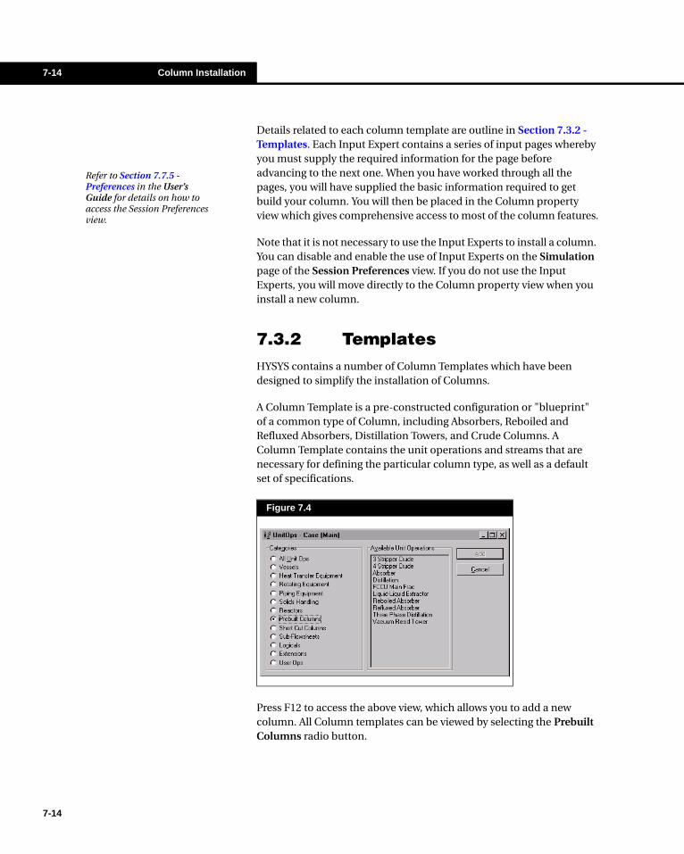
7-14 Column Installation
7-14
Details related to each column template are outline in Section 7.3.2 - Templates. Each Input Expert contains a series of input pages whereby you must supply the required information for the page before advancing to the next one. When you have worked through all the pages, you will have supplied the basic information required to get build your column. You will then be placed in the Column property view which gives comprehensive access to most of the column features.
Note that it is not necessary to use the Input Experts to install a column. You can disable and enable the use of Input Experts on the Simulation page of the Session Preferences view. If you do not use the Input Experts, you will move directly to the Column property view when you install a new column.
7.3.2 TemplatesHYSYS contains a number of Column Templates which have been designed to simplify the installation of Columns.
A Column Template is a pre-constructed configuration or "blueprint" of a common type of Column, including Absorbers, Reboiled and Refluxed Absorbers, Distillation Towers, and Crude Columns. A Column Template contains the unit operations and streams that are necessary for defining the particular column type, as well as a default set of specifications.
Press F12 to access the above view, which allows you to add a new column. All Column templates can be viewed by selecting the Prebuilt Columns radio button.
Figure 7.4
Refer to Section 7.7.5 - Preferences in the User’s Guide for details on how to access the Session Preferences view.

Column 7-15
When you add a new Column, HYSYS will give you a choice of the available templates. Simply select the template that most closely matches your column configuration, provide the necessary input in the Input Expert view (if applicable), and HYSYS will install the equipment and streams for you in a new Column subflowsheet. Stream connections will already be in place, and HYSYS will provide default names for all internal streams and equipment. You may then make modifications by adding, removing or changing the names of any streams or operations to suit your specific requirements.
Selecting the Side Ops button on the final page of the Column Input Expert will open the Side Operations Input Expert wizard which will guide you through the process of adding a side operation to your column.
In addition to the basic Column Templates which are included with HYSYS, you may create custom Templates containing Column configurations that you commonly use.
HYSYS Column Conventions
Column TRAY SECTIONS, Overhead CONDENSERS and Bottom REBOILERS are each defined as individual unit operations. Condensers and Reboilers are not numbered stages, as they are considered to be separate from the Tray Section.
The following are some of the conventions, definitions and descriptions of the basic columns:
By making the individual components of the column separate pieces of equipment, there is easier access to equipment information, as well as the streams connecting them.
Column Component Description
Tray SectionA HYSYS unit operation that represents the series of equilibrium trays in a Column. The trays are numbered from 1 to N.
Stages
Stages are numbered from the top down or from the bottom up, depending on your preference. The top tray is 1 and the bottom tray is N for the top-down numbering scheme. The stage numbering preference may be selected on the Connections page of the Design tab on the Column property view.
Overhead Vapor Product
The overhead vapor product is the vapor leaving the top tray of the Tray Section in simple Absorbers and Reboiled Absorbers. In Refluxed Absorbers and Distillation Towers, the overhead vapor product is the vapor leaving the Condenser.
Overhead Liquid Product
The overhead liquid product is the Distillate leaving the Condenser in Refluxed Absorbers and Distillation Towers. There is no top liquid product in simple Absorbers and Reboiled Absorbers.
7-15

7-16 Column Installation
7-16
Default Replaceable Specifications
Replaceable specifications are the values which the Column convergence algorithm is trying to meet. When you select a particular Column template, or as you add side equipment, HYSYS creates default specifications. You may use the specifications that HYSYS provides, or replace these specifications with others more suited to your requirements.
The available default replaceable specifications are dependent on the Basic Column type (template) that you have chosen. The default specifications for the four basic column templates are combinations of the following:
• Overhead vapor flowrate• Distillate flowrate• Bottoms flowrate• Reflux ratio• Reflux rate
The provided templates contain only pre-named internal streams (streams which are both a feed and product). For instance, the Reflux stream, which is named by HYSYS, is a product from the Condenser and a feed to the top tray of the Tray Section.
In the following schematics, you specify the feed and product streams, including duty streams.
Bottom Liquid Product
The bottom liquid product is the liquid leaving the bottom tray of the Tray Section in simple Absorbers and Refluxed Absorbers. In Reboiled Absorbers and Distillation Columns, the bottom liquid product is the liquid leaving the Reboiler.
Overhead Condenser
An Overhead Condenser represents a combined cooler and separation stage, and is not given a stage number.
Bottom ReboilerA Bottom Reboiler represents a combined heater and separation stage, and is not given a stage number.
Column Component Description
The pressure for a tray section stage, condenser or reboiler can be specified at any time on the Pressures page of the Column property view.

Column 7-17
Absorber Template
The only unit operation contained in the Absorber is the TRAY SECTION, and the only streams are the overhead vapor and bottom liquid products. A schematic representation of the Absorber appears to the left.
There are no available specifications for the Absorber, which is the base case for all tower configurations. The conditions and composition of the column Feed stream, as well as the operating pressure, will define the resulting converged solution. The converged solution includes the conditions and composition of the Vapor and Liquid Product streams.
Reboiled Absorber Template
The Reboiled Absorber template consists of a tray section and a bottom reboiler. Two additional streams connecting the REBOILER to the TRAY SECTION are also included in the template (see figure).
When you install a Reboiled Absorber (i.e. add only a REBOILER to the Tray Section), you increase the number of required specifications by one over the Base Case. As there is no overhead liquid, the default specification in this case is the overhead vapor flow rate.
Refluxed Absorber Template
The Refluxed Absorber template contains a TRAY SECTION and an overhead CONDENSER (partial or total). Additional material streams associated with the Condenser are also included in the template. For example, the vapor entering the Condenser from the top tray is named to Condenser by default, and the liquid returning to the Tray Section is the Reflux.
When you install a Refluxed Absorber, you are adding only a CONDENSER to the base case. Specifying a partial condenser increases the number of required specifications by two over the Base Case. The default specifications are the overhead vapor flow rate and the side liquid (Distillate) draw. Specifying a total condenser results in only one available specification, since there is no overhead vapor product.
The Liquid-Liquid Extraction Template is identical to the Absorber Template
The remaining Column templates have additional equipment, thus increasing the number of required specifications.
7-17

7-18 Column Installation
7-18
Either of the overhead vapor or distillate flow rates may be specified as zero, which creates three possible combinations for these two specifications. Each combination defines a different set of operating conditions. The three possible Refluxed Absorber configurations are listed below:
• Partial condenser with vapor overhead but no side liquid (distillate) draw.
• Partial condenser with both vapor overhead and distillate draws.
• Total condenser (with distillate but no vapor overhead draw).
Distillation Template
If you select the Distillation template, HYSYS will create a Column with both a REBOILER and CONDENSER. The equipment and Streams in the Distillation template are therefore a combination of the Reboiled Absorber and Refluxed Absorber Templates
Reflux Ratio
When you add both a REBOILER and a CONDENSER (Distillation), you must supply three specifications for partial condensers and two specifications for total condensers. The third default specification (in addition to Overhead Vapor Flow Rate and Side Liquid Draw) is the Reflux Ratio.
The Reflux Ratio is defined as the ratio of the liquid returning to the tray section divided by the total flow of the products (see figure). If a water draw is present, its flow is not included in the ratio.
As with the Refluxed Absorber, the Distillation template may have either a PARTIAL or TOTAL CONDENSER. Choosing a PARTIAL CONDENSER results in three replaceable specifications, while a TOTAL CONDENSER results in two replaceable specifications.
The pressure in the tower is, in essence, a replaceable specification, in that you can change the pressure for any stage from the Column property view. Note that the pressures remain fixed during the Column calculations.
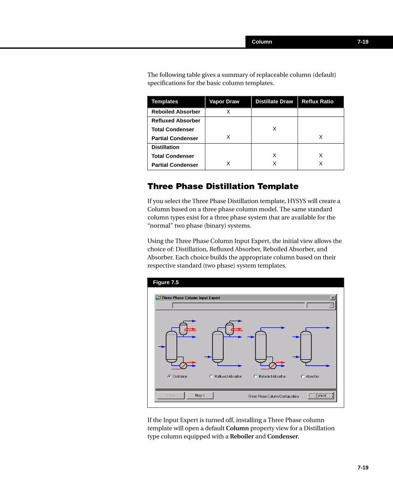
Column 7-19
The following table gives a summary of replaceable column (default) specifications for the basic column templates.
Three Phase Distillation Template
If you select the Three Phase Distillation template, HYSYS will create a Column based on a three phase column model. The same standard column types exist for a three phase system that are available for the “normal” two phase (binary) systems.
Using the Three Phase Column Input Expert, the initial view allows the choice of: Distillation, Refluxed Absorber, Reboiled Absorber, and Absorber. Each choice builds the appropriate column based on their respective standard (two phase) system templates.
If the Input Expert is turned off, installing a Three Phase column template will open a default Column property view for a Distillation type column equipped with a Reboiler and Condenser.
Templates Vapor Draw Distillate Draw Reflux Ratio
Reboiled Absorber X
Refluxed Absorber
Total Condenser
Partial Condenser X
X
X
Distillation
Total Condenser
Partial Condenser X
X
X
X
X
Figure 7.5
7-19

7-20 Column Property View
7-20
The key difference between using the standard column templates and their three phase counterparts lies in the solver that is used. The default solver for three phase columns is the “Sparse Continuation” solver which is an advanced solver designed to handle three phase, non ideal chemical systems, that other solvers cannot.
When using the Three Phase Column Input Expert some additional specifications may be required when compared with the standard (binary system) column setups. An Azeotropic Input Expert is also integrated into the setup which can is accessible by selecting the Azeotropic Initialization button from the final Specifications setup page of the Input Expert.
Selecting the Side Ops button on the final page of the Three Phase Column Input Expert will open the Side Operations Input Expert wizard which will guide you through the process of adding a side operation to your column.
Three phase distillation columns are notoriously difficult to solve, and thus the Input Experts are designed to properly initialize temperatures, flows and compositions to aid in convergence of the tower.
7.4 Column Property ViewThe Column property view is a book of tabs containing pages with information pertaining to the Column, which is accessible from the main flowsheet or Column subflowsheet. In the Column subflowsheet, the Column property view is also known as the Column Runner, and can be accessed by selecting the Column Runner button.
The Column property view is used to define specifications, provide estimates, monitor convergence, view stage-by-stage and product stream summaries, add pump-arounds and side-strippers, specify dynamic parameters and define other Column parameters such as convergence tolerances and attach reactions to column stages.
The Column property view is essentially the same when accessed from the main flowsheet or Column subflowsheet. However, there are some differences:
• The Connections page in the Main flowsheet Column property view displays and allows you to change all product and feed stream connections. In addition, you can specify the number of stages and condenser type.
It requires some expertise to set up, initialize and solve three phase distillation problems. Additional modeling software applications such as DISTIL, use residue curve maps and distillation region diagrams to determine feasible designs and can greatly assist in the initial design work. Contact your local Hyprotech representative for details.
Column Runner is another name for the subflowsheet Column property view.
Column Runner Button
There are some differences in the Column property view in the main flowsheet and in the Column subflowsheet. These differences will be noted.
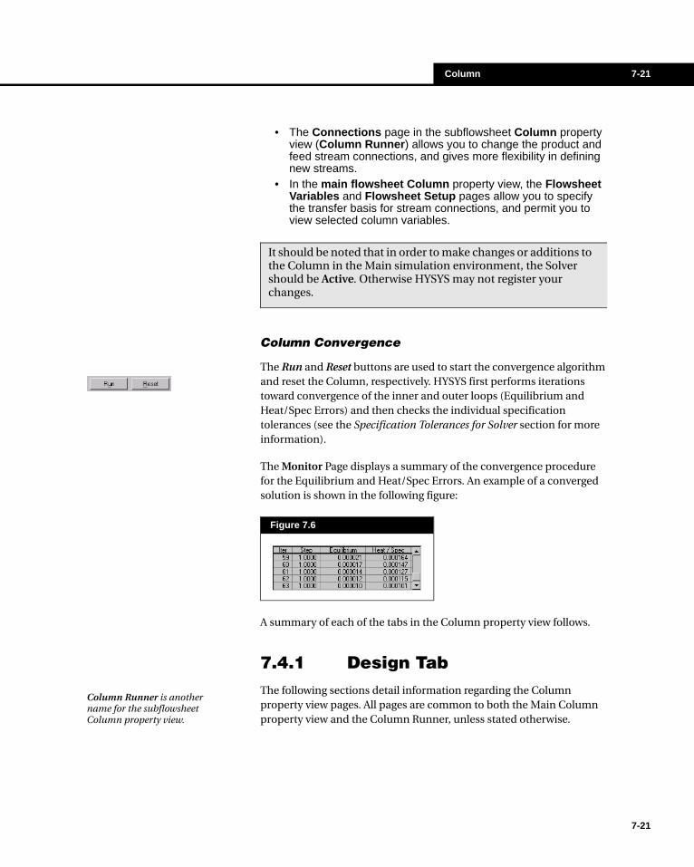
Column 7-21
• The Connections page in the subflowsheet Column property view (Column Runner) allows you to change the product and feed stream connections, and gives more flexibility in defining new streams.
• In the main flowsheet Column property view, the Flowsheet Variables and Flowsheet Setup pages allow you to specify the transfer basis for stream connections, and permit you to view selected column variables.
Column Convergence
The Run and Reset buttons are used to start the convergence algorithm and reset the Column, respectively. HYSYS first performs iterations toward convergence of the inner and outer loops (Equilibrium and Heat/Spec Errors) and then checks the individual specification tolerances (see the Specification Tolerances for Solver section for more information).
The Monitor Page displays a summary of the convergence procedure for the Equilibrium and Heat/Spec Errors. An example of a converged solution is shown in the following figure:
A summary of each of the tabs in the Column property view follows.
7.4.1 Design TabThe following sections detail information regarding the Column property view pages. All pages are common to both the Main Column property view and the Column Runner, unless stated otherwise.
Figure 7.6
It should be noted that in order to make changes or additions to the Column in the Main simulation environment, the Solver should be Active. Otherwise HYSYS may not register your changes.
Column Runner is another name for the subflowsheet Column property view.
7-21

7-22 Column Property View
7-22
Connections page (Main Flowsheet)
The main flowsheet Connections page allows you to specify the name and location of feed streams, the number of stages in the tray section, the stage numbering scheme, condenser type, names of the Column product streams and Condenser/Reboiler energy streams. Note that the streams shown in this view reside in the parent or main flowsheet; they do not include Column subflowsheet streams, such as the Reflux or Boilup. In other words, only feed and product streams (material and energy) are displayed on this page.
Note that if you have modified the Column Template (e.g. - added an additional Tray Section), the Connections page will appear differently than what is shown in Figure 7.7.
Figure 7.7
The appearance of the Connections page will vary depending on the template you are using.

Column 7-23
Connections page (Column Runner)
The Connections page displayed in the Column Runner (inside the Column subflowsheet) appears as shown in the following figure.
All Feed and Energy Streams, as well as the associated stage, are displayed in the left portion of the Connections page. Liquid, Vapor and Water Product streams and locations are displayed on the right-hand side of the page.
Monitor Page
The Monitor page is primarily used for editing specifications, monitoring Column convergence and viewing Column profile plots. An input summary and a view of the initial estimates can also be accessed from this page.
Figure 7.8If you specify a new stream name in any of the cells, this creates the stream inside the Column. This new stream is not automatically transferred into the main flowsheet.
You can connect or disconnect streams from this page, as well as change the stream location.
7-23

7-24 Column Property View
7-24
Figure 7.9
HYSYS will display the iteration number, step size and Equilibrium and Heat/Spec errors in this area during the iteration process.
Profiles are where plots of column temperatures, flows and pressures are displayed during convergence.
Specification types, the value of each specification, the current calculated value and the weighted error are displayed here.
Buttons for working with specifications.
The Current checkboxshows the current specs that are being used in the column solution. The user cannot check this box.

Column 7-25
Optional Checks Group
In the Optional Checks group, you will find the following two buttons:
Profile Group
During the column calculations, a profile of temperature, pressure or flow will be displayed and updated as the solution progresses. Select the appropriate radio button to display the desired variable versus tray number profile.
Specifications Group
Each specification, along with its specified value, current value, weighted error and status is shown in the Specifications group.
You can change a specified value by typing directly in the associated Specified Value cell. Specified values can also be viewed and changed on the Specs and Specs Summary pages. Any changes made in one location will be reflected across all locations. See Section 7.5 - Column Specification Types for a description of the available specification types.
Double clicking on a cell within the row for any listed specification will open its property view. In this view, you define all the information associated with a particular specification. Each specification view has three tabbed pages: Parameters, Summary and Spec Type. This view can also be accessed from both the Specs and Specs Summary pages. Further details are outlined in following Specification Property View sub section.
Button Function
Input Summary
This button will provide a column input summary in the Trace Window. The summary lists vital tower information including the number of trays, the attached Fluid Package, attached streams and specifications.
You can press the Input Summary button after you make a change to any of the column parameters to view an updated input summary. The newly defined column configuration will be displayed.
View Initial Estimates
This button will open the Summary page of the Column property view and display initial temperature and flow estimates for the column. You can then use the values generated by HYSYS to enter estimates on the Est. page.
These estimates are generated by performing one iteration using the current column configuration. If a specification for flow or temperature has been provided, it will be honoured in the displayed estimates.
Refer to Section 5.4 - Object Status Window/Trace Window in the User’s Guide for details concerning the Trace Window.
New specifications are added via the Specs page.
7-25

7-26 Column Property View
7-26
Spec Status Check Boxes
The status of listed specifications will be one of the following types:
The degrees of freedom value is displayed in the Degrees of Freedom field on the Monitor page. When you make a specification active, the degrees of freedom is decreased by one. Conversely, when you de-activate a specification, the degrees of freedom is increased by one. You can start column calculations when there are zero degrees of freedom.
Note that variables such as the duty of the reboiler stream, which is specified in the Workbook, or feed streams that are not completely known will offset the current degrees of freedom. If you feel that the number of active specifications is appropriate for the current configuration, yet the degrees of freedom is not zero, check the conditions of the attached streams (material and energy).You must provide as many specifications as there are available degrees of freedom. For a simple Absorber there are no available degrees of freedom, therefore no specifications are required. Distillation columns with a partial condenser have three available degrees of freedom.
Spec Status Check Boxes
Status Description
Active
The active specification is one that the convergence algorithm is trying to meet. Note that an active specification always serves as an initial estimate (when the Active box is checked, HYSYS automatically checks the Estimate and Current boxes). An active specification always exhausts one degree of freedom.
Estimate
An Estimate is considered an Inactive specification because the convergence algorithm is not trying to satisfy it. To use a specification as an estimate only, clear the Active box by selecting it. The value will then serve only as an initial estimate for the convergence algorithm. An estimate does not exhaust an available degree of freedom.
Current
This check box shows the current specs being used by the column solution. When the Active box is checked, the Current box will automatically be checked. The user cannot alter this check box.
When Alternate specs are used and an existing hard to solve spec has been replaced with an Alternate spec, this check box makes it clear to the user the current specs used to solve the column.
Completely Inactive
To disregard the value of a specification entirely during convergence, clear both the Active and Estimate check boxes. By ignoring a specification rather than deleting it, you will always be able to use it later if required. The current value will be displayed for each specification, regardless of its status. An Inactive specification is therefore ideal when you want to monitor a key variable without including it as an estimate or specification.
An Active specification is one which the convergence algorithm is trying to meet initially. An Active specification has the Estimate check box selected also.
An Estimate is used as an initial "guess" for the convergence algorithm, and is considered to be an Inactive specification.
A Current specification is one which is currently being used in the column solution.
A Completely Inactive specification is ignored completely by the convergence algorithm, but may be made Active or an Estimate at a later time.
Column 7-27
Specification Group Buttons
The four buttons which align the bottom of the Specifications group allow you to manipulate the list of specs:
Specs Page
Adding and changing Column specifications is straightforward. If you have created a Column based on one of the templates, HYSYS already has default specifications in place. The type of default specification depends on which of the templates you have chosen (see the Default Replaceable Specifications sub section in Section 7.3.2 - Templates) for more details.
Button Action
View...
Move to one of the specification cells and select the View button to display its property view. You may then make any necessary changes to the specification. See the following Specification Property View sub section for more details.
To change the value of a specification only, move to the Specified Value input cell for the specification you wish to change, and type in the new value.
Add Spec...
Opens the Column Specifications menu list, from which you can select one or multiple (by holding the CTRL key while selecting) specifications and then press the Add Spec(s) button.
The property view for each new spec will be shown and its name will be added to the list of existing specifications. See the following 7.5Column Specification Types sub section for a description of the available specification types.
Update Inactive Updates the specified value of each inactive specification with its current value.
Group Active Arranges all active specifications together at the top of the specifications list.
You can also double click in a specification cell to open its property view.
7-27

7-28 Column Property View
7-28
Column Specifications Group
The following buttons are available:
From the Default Basis drop down list, you can choose the basis of new specifications to be Molar, Mass or Volume.
The Update Specs from Dynamics button will replace the Specified Value of each specification with the Current Value (lined out value) obtained from dynamics mode.
Specification Property View
Shown below is a typical property view of a specification. In this view, you define all the information associated with a particular specification. Each specification has three tabbed pages: Parameters, Summary, and Spec Type. This example shows a component recovery specification which requires the Stage Number, Spec Value, and Phase type when a Target Type of Stage is chosen.
Note that specification information is shared between this property view and the specification list on both the Monitor and Specs Summary pages. Altering information in one location will automatically update across all other locations. For example, you may
Button Action
View
Opens the property view for the highlighted specification. Alternatively, you can object inspect a spec name and select View from the menu. See the following Specification Property View sub section for more details.
Add
Opens the Column Specifications menu list, from which you can select one or multiple (by holding the CTRL key while selecting) specifications and then press the Add Spec(s) button.
The property view for each new spec will be shown and its name will be added to the list of existing specifications. See Section 7.5 - Column Specification Types for a description of the available specification types.
Delete Removes the highlighted specification from the list.
Available Specification TypesNote that you are only able to add Column Stream Specifications via the Stream Property View of a draw stream within the Column subflowsheet.
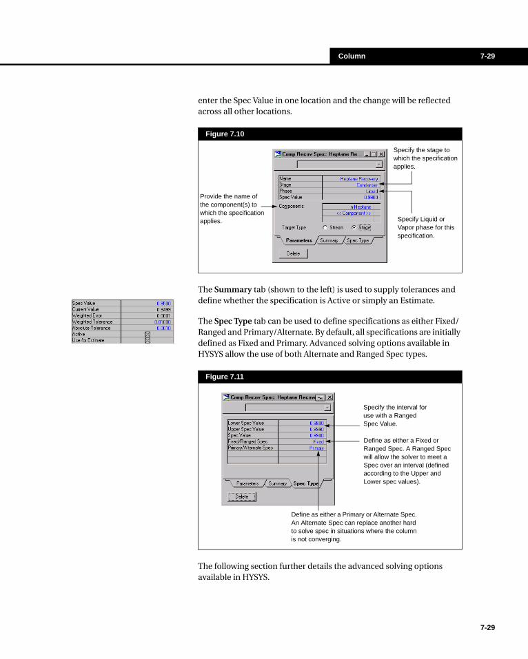
Column 7-29
enter the Spec Value in one location and the change will be reflected across all other locations.
The Summary tab (shown to the left) is used to supply tolerances and define whether the specification is Active or simply an Estimate.
The Spec Type tab can be used to define specifications as either Fixed/Ranged and Primary/Alternate. By default, all specifications are initially defined as Fixed and Primary. Advanced solving options available in HYSYS allow the use of both Alternate and Ranged Spec types.
The following section further details the advanced solving options available in HYSYS.
Figure 7.10
Figure 7.11
Specify the stage to which the specification applies.
Specify Liquid or Vapor phase for this specification.
Provide the name of the component(s) to which the specification applies.
Specify the interval for use with a Ranged Spec Value.
Define as either a Fixed or Ranged Spec. A Ranged Spec will allow the solver to meet a Spec over an interval (defined according to the Upper and Lower spec values).
Define as either a Primary or Alternate Spec. An Alternate Spec can replace another hard to solve spec in situations where the column is not converging.
7-29

7-30 Column Property View
7-30
Ranged and Alternate Specs
The reliability of any solution method depends on its ability to solve a wide group of problems. Some specs like purity, recovery and cut point are hard to solve compared to a flow or reflux ratio spec. The use of Alternate and/or Ranged Specs can help to solve columns that fail due to difficult specifications.
Configuration of these advanced solving options are made by selecting the Advanced Solving Options button located on the Solver page. The advanced solving options are only available for use with either the Hysim I/O or Modified I/O solving methods. See the Advanced Solving Options Button sub section in Section 7.4.2 - Parameters Tabfor further details.
Fixed/Ranged Specs
A Fixed Spec is one which HYSYS attempts to solve for a specific value. For a Ranged Spec, the solver attempts to meet the specified value, but if the rest of the specifications are not solved after a set number of iterations, the spec is perturbed within the interval until the column converges. Any column specification can be specified over an interval. A Ranged Spec requires both Lower and Upper specification values to be entered. This option (when enabled), may help solve columns where some specifications can be varied over an interval to meet the rest of the specifications.
Primary/Alternate Specs
A Primary Spec is one which must be met for the column solution to converge. An Alternate Spec can be used to replace an existing hard to solve specification during a column solution. The solver first attempts to meet an active Alternate spec value, but if the rest of the specifications are not solved after a minimum number of iterations, the active Alternate spec is replaced by an inactive Alternate spec. This option (when enabled), may help solve columns where some specifications can be ignored (enabling another) to meet the rest of the specifications and converge the column.
If the Column solves on an Alternate or Ranged Spec, the status bar will read “Converged - Alternate Specs” highlighted in purple.
When the solver attempts to meet a Ranged spec, the Wt. Error will become zero when the Current Value is within the Ranged interval (as shown on the Monitor page).
When an existing spec is replaced by an alternate spec during a column solution, the Current check box becomes un-checked for the original (not met) spec and is checked for the alternate spec.
The number of active Alternate specs must always equal the number of inactive Alternate specs.
Note that both Ranged or Alternate Specs must be enabled and configured using the Advanced Solving Options Button located on the Solver page of the Parameters tab before they can be applied during a column solution.

Column 7-31
Specification Tolerances for Solver
The Solver Tolerances feature has been provided to allow you to specify individual tolerances for your Column specifications. In addition to HYSYS converging to a solution for the Heat/Spec and Equilibrium Errors, the individual specification tolerances must also be satisfied. HYSYS first performs iterations until the Heat/Spec (inner loop) and Equilibrium (outer loop) errors are within specified tolerances (described in the Section 7.4.2 - Parameters Tab).
The Column specifications do not have individual tolerances during this initial iteration process; the specification errors are "lumped" into the Heat/Spec Error. Once the Heat/Spec and Equilibrium conditions are met, HYSYS proceeds to compare the error with the tolerance for each individual specification. If any of these tolerances are not met, HYSYS iterates through the Heat/Spec and Equilibrium loops again to produce another converged solution. The specification errors and tolerances are again compared, and the process continues until both the inner/outer loops and the specification criteria are met.
Specific Solver Tolerances may be provided for each individual specification. HYSYS calculates two kinds of errors for each specification: an absolute error and a weighted error. The absolute error is simply the absolute value of the difference between the calculated and specified values:
The Weighted Error is a function of the particular specification type.
When a specification is active, the convergence algorithm is trying to meet the Weighted Tolerances (Absolute Tolerances are only used if no Weighted Tolerances are specified). Therefore, both the weighted and absolute errors must be less than their respective tolerances for an active specification to converge. HYSYS provides default values for all specification tolerances, but any tolerance can be changed. For example, if you are dealing with ppm levels of crucial components, composition tolerances may be set tighter (smaller) than the other specification tolerances. If you delete any tolerances, HYSYS will not apply the individual specification criteria to that specification, and Ignore will appear in the tolerance input cell.
The specification tolerance feature is simply an "extra" to permit you to work with individual specifications and change their tolerances if desired.
Errorabsolute = |Calculated Value - Specified Value| (7.1)
When the Weighted and Absolute Errors are less than their respective tolerances, an Active specification has converged.
7-31

7-32 Column Property View
7-32
Specification Details Group
For a highlighted specification in the Column Specifications group, the following information will be displayed:
• Spec Name• Convergence Condition - if the weighted and absolute errors
are within their tolerances, the specification has converged and Yes will be displayed.
• Status - you can manipulate the Active and Use As Estimate check boxes. See the Monitor Page for further details concerning the use of these check boxes.
• Spec Type - you can select between Fixed/Ranged and Primary/Alternate specs. See the Ranged and Alternate Specs sub section for more details.
• Specified and Current Calculated Values.• Weighted/Absolute Tolerance and Calculated Error.
Specs Summary Page
The Specs Summary page lists all Column specifications available along with relevant information. This specification information is shared with the Monitor and Specs Summary pages. Altering information in one location will automatically update across all other locations.
Subcooling Page
The Subcooling page allows you to specify subcooling for products coming off the condenser of your column. You can specify the condenser product temperature or the degrees to subcool. For columns without condensers, such as absorbers, this page requires no additional information.
Figure 7.12
You can edit any specification values shown in blue.
You can edit any specification details shown in blue.
You can also double click in a specification cell to open its property view. See the Specification Property View sub section for more details
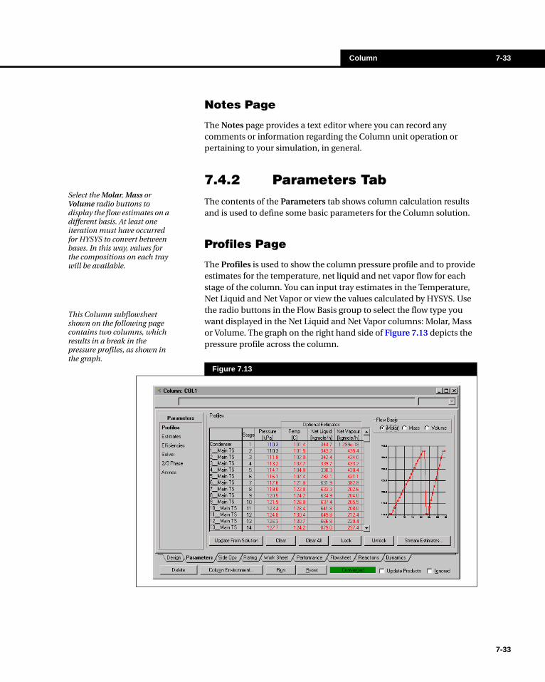
Column 7-33
7-33
Notes Page
The Notes page provides a text editor where you can record any comments or information regarding the Column unit operation or pertaining to your simulation, in general.
7.4.2 Parameters TabThe contents of the Parameters tab shows column calculation results and is used to define some basic parameters for the Column solution.
Profiles Page
The Profiles is used to show the column pressure profile and to provide estimates for the temperature, net liquid and net vapor flow for each stage of the column. You can input tray estimates in the Temperature, Net Liquid and Net Vapor or view the values calculated by HYSYS. Use the radio buttons in the Flow Basis group to select the flow type you want displayed in the Net Liquid and Net Vapor columns: Molar, Mass or Volume. The graph on the right hand side of Figure 7.13 depicts the pressure profile across the column.
This Column subflowsheet shown on the following page contains two columns, which results in a break in the pressure profiles, as shown in the graph.
Select the Molar, Mass or Volume radio buttons to display the flow estimates on a different basis. At least one iteration must have occurred for HYSYS to convert between bases. In this way, values for the compositions on each tray will be available.
Figure 7.13

7-34 Column Property View
7-34
The buttons at the bottom of the view are defined as follows:
Estimates Page
The Estimates page is used to view and provide composition estimates. Estimates are NOT a requirement for convergence.
When you provide estimates on stages that are not adjacent to each other, HYSYS will not interpolate values for intermediate stages until the solution algorithm begins.
On this view, you can provide tray by tray component composition estimates for the vapor phase or liquid phase. Each composition estimate is on a mole fraction basis, so values must be between 0 and 1.
Profiles Button Function
Update from Solution
Transfers the current values that HYSYS has calculated for the trays into the appropriate cells. Estimates that have been Locked (displayed in blue) will not be updated.
Clear Deletes values for selected tray.
Clear All Deletes values for all trays.
Lock
Changes all red values (unlocked estimates, current values, interpolated values) to blue (locked), which means that they will not be overwritten by current values when the Update from Solution button is pressed.
UnlockChanges all blue values (locked) to red (unlocked). Unlocked values will be overwritten by current values when the Update from Solutions button is pressed.
Stream Estimates
Displays the temperature, molar flow and enthalpy of all streams attached to the column operation.
Figure 7.14
To see the initial estimates generated by HYSYS, press the View Initial Estimates button on the Monitor page.
Estimates are NOT required for column convergence.
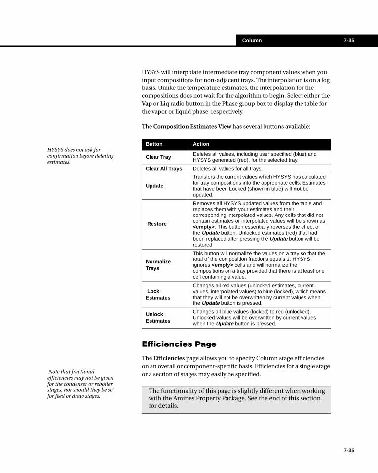
Column 7-35
HYSYS will interpolate intermediate tray component values when you input compositions for non-adjacent trays. The interpolation is on a log basis. Unlike the temperature estimates, the interpolation for the compositions does not wait for the algorithm to begin. Select either the Vap or Liq radio button in the Phase group box to display the table for the vapor or liquid phase, respectively.
The Composition Estimates View has several buttons available:
Efficiencies Page
The Efficiencies page allows you to specify Column stage efficiencies on an overall or component-specific basis. Efficiencies for a single stage or a section of stages may easily be specified.
HYSYS does not ask for confirmation before deleting estimates.
Button Action
Clear Tray Deletes all values, including user specified (blue) and HYSYS generated (red), for the selected tray.
Clear All Trays Deletes all values for all trays.
Update
Transfers the current values which HYSYS has calculated for tray compositions into the appropriate cells. Estimates that have been Locked (shown in blue) will not be updated.
Restore
Removes all HYSYS updated values from the table and replaces them with your estimates and their corresponding interpolated values. Any cells that did not contain estimates or interpolated values will be shown as <empty>. This button essentially reverses the effect of the Update button. Unlocked estimates (red) that had been replaced after pressing the Update button will be restored.
Normalize Trays
This button will normalize the values on a tray so that the total of the composition fractions equals 1. HYSYS ignores <empty> cells and will normalize the compositions on a tray provided that there is at least one cell containing a value.
Lock Estimates
Changes all red values (unlocked estimates, current values, interpolated values) to blue (locked), which means that they will not be overwritten by current values when the Update button is pressed.
Unlock Estimates
Changes all blue values (locked) to red (unlocked). Unlocked values will be overwritten by current values when the Update button is pressed.
Note that fractional efficiencies may not be given for the condenser or reboiler stages, nor should they be set for feed or draw stages.
The functionality of this page is slightly different when working with the Amines Property Package. See the end of this section for details.
7-35
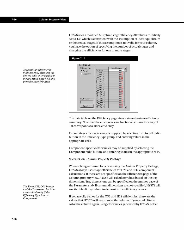
7-36 Column Property View
7-36
HYSYS uses a modified Murphree stage efficiency. All values are initially set to 1.0, which is consistent with the assumption of ideal equilibrium or theoretical stages. If this assumption is not valid for your column, you have the option of specifying the number of actual stages and changing the efficiencies for one or more stages.
The data table on the Efficiency page gives a stage-by-stage efficiency summary. Note that the efficiencies are fractional, i.e. an efficiency of 1.0 corresponds to 100% efficiency.
Overall stage efficiencies may be supplied by selecting the Overall radio button in the Efficiency Type group, and entering values in the appropriate cells.
Component-specific efficiencies may be supplied by selecting the Component radio button, and entering values in the appropriate cells.
Special Case - Amines Property Package
When solving a column for a case using the Amines Property Package, HYSYS always uses stage efficiencies for H2S and CO2 component calculations. If these are not specified on the Efficiencies page of the Column property view, HYSYS will calculate values based on the tray dimensions. Tray dimensions can be specified on the Amines page of the Parameters tab. If column dimensions are not specified, HYSYS will use its default tray values to determine the efficiency values.
If you specify values for the CO2 and H2S efficiencies, these are the values that HYSYS will use to solve the column. If you would like to solve the column again using efficiencies generated by HYSYS, select
Figure 7.15
To specify an efficiency to multiple cells, highlight the desired cells, enter a value in the Eff. Multi-Spec field and press the Specify button.
The Reset H2S, CO2 button and the Transpose check box are available only if the Efficiency Type is set to Component.
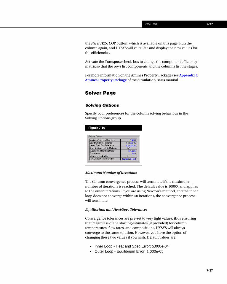
Column 7-37
the Reset H2S, CO2 button, which is available on this page. Run the column again, and HYSYS will calculate and display the new values for the efficiencies.
Activate the Transpose check-box to change the component efficiency matrix so that the rows list components and the columns list the stages.
For more information on the Amines Property Packages see Appendix C Amines Property Package of the Simulation Basis manual.
Solver Page
Solving Options
Specify your preferences for the column solving behaviour in the Solving Options group.
Maximum Number of Iterations
The Column convergence process will terminate if the maximum number of iterations is reached. The default value is 10000, and applies to the outer iterations. If you are using Newton’s method, and the inner loop does not converge within 50 iterations, the convergence process will terminate.
Equilibrium and Heat/Spec Tolerances
Convergence tolerances are pre-set to very tight values, thus ensuring that regardless of the starting estimates (if provided) for column temperatures, flow rates, and compositions, HYSYS will always converge to the same solution. However, you have the option of changing these two values if you wish. Default values are:
• Inner Loop - Heat and Spec Error: 5.000e-04• Outer Loop - Equilibrium Error: 1.000e-05
Figure 7.16
7-37

7-38 Column Property View
7-38
Because the default values are already very small, you should use caution in making them any smaller. You should not make these tolerances looser (larger) for preliminary work to reduce computer time. The time savings are usually minor, if any. Also, if the column is in a recycle or adjust loop, this could cause difficulty for the loop convergence.
Equilibrium Error
The value of the equilibrium error printed during the column iterations represents the error in the calculated vapor phase mole fractions. The error over each stage is calculated as one minus the sum of the component vapor phase mole fractions. This value is then squared; the total equilibrium error is the sum of the squared values. The total equilibrium error must be less than 0.00001 to be considered a converged column.
Heat and Spec Error
The heat and specification error is the sum of the absolute values of the heat error and the specification error, summed over each stage in the tower.
This total value is divided by the number of inner loop equations. The heat error contribution is the heat flow imbalance on each tray divided by the total average heat flow through the stage.
The specification error contribution is the sum of each individual specification error divided by an appropriate normalization factor.
For component(s) flow, the normalization factor is the actual component(s) flow; for composition, it is the actual mole fraction; for vapor pressure and temperature it is a value of 5000; etc. The total sum of heat and spec errors must be less than 0.0005 to be considered a converged column.
The allowed equilibrium error and heat and spec error are tighter than in most programs, but this is necessary to avoid meta-stable solutions and to ensure satisfactory column heat and material balances.
Save Solution as Initial Estimate
This option is on by default, and it saves converged solutions as estimates for the next solution.

Column 7-39
Super Critical Handling Model
Supercritical phase behaviour occurs when one or more Column stages are operating above the critical point of one or more components. During the convergence process, supercritical behaviour may be encountered on one or more stages in the Column. If HYSYS encounters supercritical phase behaviour, appropriate messages will be displayed in the Trace Window.
HYSYS cannot use the equation of state or activity model in the supercritical range, so an alternate method must be used. You may specify which method you wish HYSYS to use to model the phase behaviour. There are three choices for supercritical calculations:
Trace Level
The Trace Level defines the level of detail for messages displayed in the Trace Window and may be set to Low, Medium or High. The default is Low.
Initialize from Ideal K’s
When this check box is activated, HYSYS initializes its column solution using ideal K values which are calculated from vapor pressure correlations. The ideal K-value option, which is also used by HYSIM, increases the compatibility between HYSIM and HYSYS.
Model Description
Simple K
This is the default method. HYSYS calculates K-values for the components based on the vapor pressure model being used. Using this method, the K-values which are calculated are ideal K-values.
Decrease Pressure
When supercritical conditions are encountered, HYSYS reduces the pressure on all trays by an internally determined factor, which can be seen in the Trace Window when the Verbose option is used. This factor is gradually decreased until supercritical conditions no longer exist on any tray, at which point, the pressure in the column is gradually increased to the user specified pressure. If supercritical conditions are encountered during the pressure increase, the pressure is once again reduced and the process is repeated.
Adjacent Tray
When supercritical conditions are encountered on a tray, HYSYS searches for the closest tray above which does not have supercritical behaviour. The non-supercritical conditions are substituted in the phase calculations for the tray with supercritical conditions.
See Section 5.4 - Object Status Window/Trace Window in the User’s Guide for details on the Trace Window.
7-39

7-40 Column Property View
7-40
By default, the Initialize from Ideal K’s check box is cleared. HYSYS uses specified composition estimates or generates estimates to rigorously calculate K-values.
Two Liquids Check Based on
This option allows you to specify a check for two liquid phases in the column. The check is based on one of the following criteria:
• No. 2 Liq Check - disables the two liquid check• Tray Liquid Fluid - the calculation is based on the composition
of the liquid in the column• Tray Total Fluid - the calculation is based on the overall
composition of the fluid in the column
Solving Method
The Solving Method drop down list allows you to select the column solution method.
The text box, which is displayed below the drop down list, provides explanations for each method, and is restated here:
Figure 7.17
Method Explanation
HYSIM Inside-Out General purpose method which is good for most problems.
Modified HYSIM Inside-Out
General purpose method which allows mixer, tee and heat exchangers inside the column subflowsheet.
Newton Raphson Inside-Out
General purpose method which allows liquid-phase kinetic reactions inside the Column subflowsheet.
Sparse Continuation Solver
This is an equation based solver. It supports two liquid phases on the trays and its main use is for solving highly non-ideal chemical systems and reactive distillation.
Simultaneous Correction
Simultaneous method using dogleg methods. Good for chemical systems. This method also supports reactive distillation.
Only a simple Heat Exchanger Model (Calculated from Column) is available in the Column subflowsheet. The Simple Rating, End-Point and Weighted models are not available.
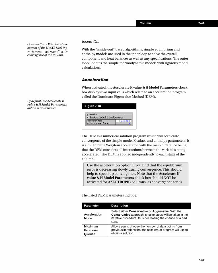
Column 7-41
Inside-Out
With the "inside-out" based algorithms, simple equilibrium and enthalpy models are used in the inner loop to solve the overall component and heat balances as well as any specifications. The outer loop updates the simple thermodynamic models with rigorous model calculations.
Acceleration
When activated, the Accelerate K value & H Model Parameters check box displays two input cells which relate to an acceleration program called the Dominant Eigenvalue Method (DEM).
The DEM is a numerical solution program which will accelerate convergence of the simple model K values and enthalpy parameters. It is similar to the Wegstein accelerator, with the main difference being that the DEM considers all interactions between the variables being accelerated. The DEM is applied independently to each stage of the column.
The listed DEM parameters include:
Figure 7.18
Open the Trace Window at the bottom of the HYSYS DeskTop to view messages regarding the convergence of the column.
By default, the Accelerate K value & H Model Parameters option is de-activated.
Use the acceleration option if you find that the equilibrium error is decreasing slowly during convergence. This should help to speed up convergence. Note that the Accelerate K value & H Model Parameters check box should NOT be activated for AZEOTROPIC columns, as convergence tends
Parameter Description
Acceleration Mode
Select either Conservative or Aggressive. With the Conservative approach, smaller steps will be taken in the iterative procedure, thus decreasing the chance of a bad step.
Maximum Iterations Queued
Allows you to choose the number of data points from previous iterations that the accelerator program will use to obtain a solution.
7-41
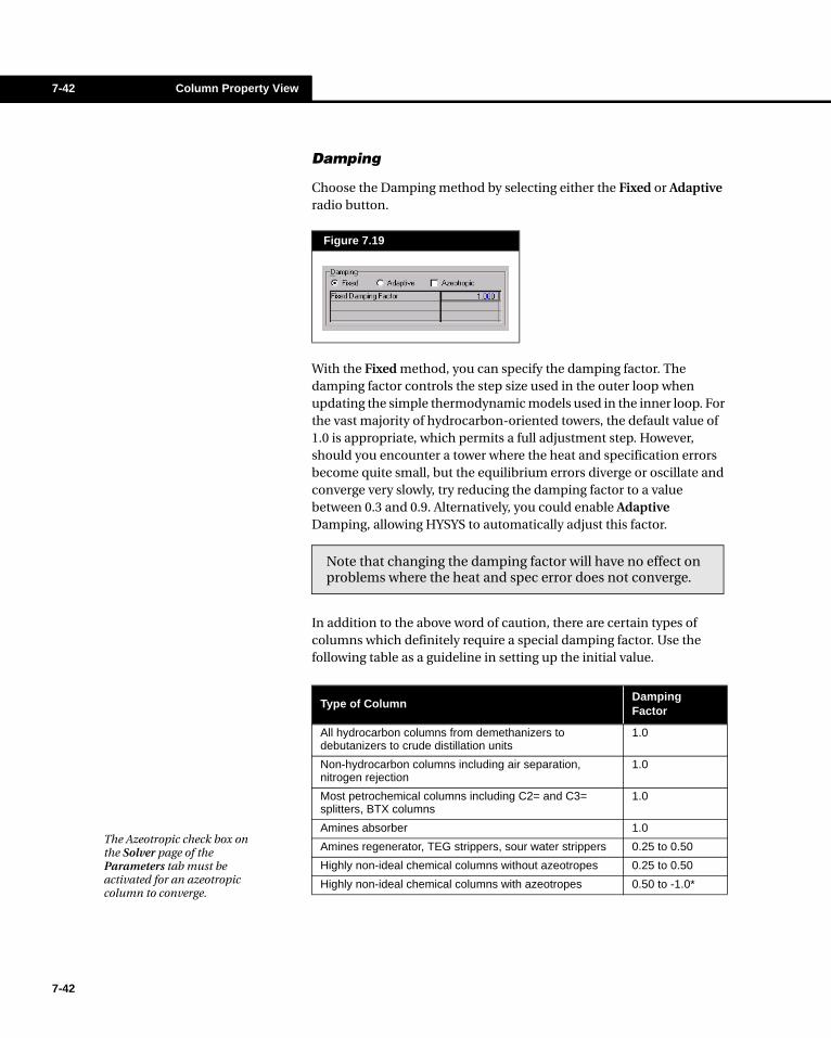
7-42 Column Property View
7-42
Damping
Choose the Damping method by selecting either the Fixed or Adaptive radio button.
With the Fixed method, you can specify the damping factor. The damping factor controls the step size used in the outer loop when updating the simple thermodynamic models used in the inner loop. For the vast majority of hydrocarbon-oriented towers, the default value of 1.0 is appropriate, which permits a full adjustment step. However, should you encounter a tower where the heat and specification errors become quite small, but the equilibrium errors diverge or oscillate and converge very slowly, try reducing the damping factor to a value between 0.3 and 0.9. Alternatively, you could enable Adaptive Damping, allowing HYSYS to automatically adjust this factor.
In addition to the above word of caution, there are certain types of columns which definitely require a special damping factor. Use the following table as a guideline in setting up the initial value.
Figure 7.19
Note that changing the damping factor will have no effect on problems where the heat and spec error does not converge.
Type of ColumnDamping Factor
All hydrocarbon columns from demethanizers to debutanizers to crude distillation units
1.0
Non-hydrocarbon columns including air separation, nitrogen rejection
1.0
Most petrochemical columns including C2= and C3= splitters, BTX columns
1.0
Amines absorber 1.0
Amines regenerator, TEG strippers, sour water strippers 0.25 to 0.50
Highly non-ideal chemical columns without azeotropes 0.25 to 0.50
Highly non-ideal chemical columns with azeotropes 0.50 to -1.0*
The Azeotropic check box on the Solver page of the Parameters tab must be activated for an azeotropic column to converge.

Column 7-43
As shown in the previous table, an azeotropic column requires that the azeotrope check be enabled. There are two ways to indicate to HYSYS that you are simulating an azeotropic column:
1. Enter a negative damping factor, and HYSYS will automatically select the Azeotropic check box. Note that the absolute value of the damping factor is always displayed.
2. Enter a positive value for the damping factor and select the Azeotropic check box.
Adaptive Damping
If you select the Adaptive radio button, the Damping matrix will display three fields. HYSYS will update the damping factor as the column solution is calculated, depending on the Damping Period and convergence behaviour.
Initial Estimate Generator Parameters
You can enable the initial estimate generator (IEG) by activating the Dynamic Integration for IEG check box. The IEG will then perform iterative flash calculations (NRSolver, PV and PH) to provide initial estimates for the temperature and composition profiles. No user estimates are required when the Dynamic Integration for IEG check box is activated.
Damping Period Description
Initial Damping Factor
Specifies the starting point for adaptive damping.
Adaptive Damping Period
The default Adaptive Damping Period is ten. In this case, after the tenth iteration, HYSYS will look at the last ten errors to see how many times the error increased rather than decreased. If the error increased more than the acceptable tolerance, this is an indication that the convergence is likely cycling, and the current damping factor is then multiplied by 0.7. Every ten iterations, the same analysis is done to see if the damping factor should be further decreased. Alternatively, if the error increased only once in the last period, the damping factor is increased to allow for quicker convergence.
Update Initial Damping Factor
If this option is checked, the current damping factor will be used the next time the column is solved. If it is not checked, the damping factor before adaptive damping was applied will be used.
Figure 7.20
7-43
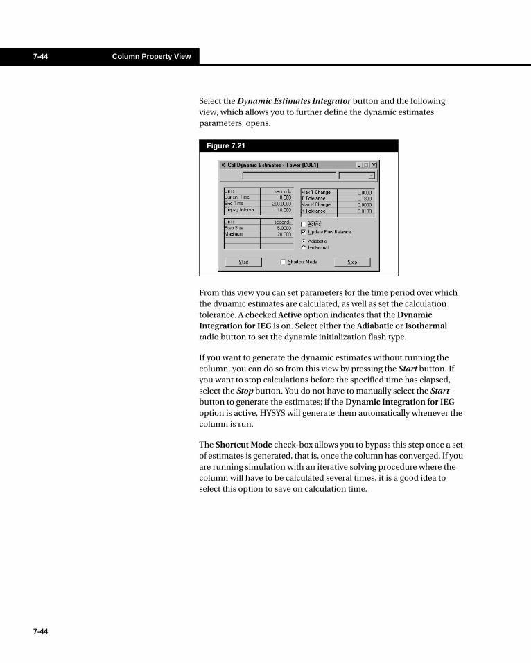
7-44 Column Property View
7-44
Select the Dynamic Estimates Integrator button and the following view, which allows you to further define the dynamic estimates parameters, opens.
From this view you can set parameters for the time period over which the dynamic estimates are calculated, as well as set the calculation tolerance. A checked Active option indicates that the Dynamic Integration for IEG is on. Select either the Adiabatic or Isothermal radio button to set the dynamic initialization flash type.
If you want to generate the dynamic estimates without running the column, you can do so from this view by pressing the Start button. If you want to stop calculations before the specified time has elapsed, select the Stop button. You do not have to manually select the Start button to generate the estimates; if the Dynamic Integration for IEG option is active, HYSYS will generate them automatically whenever the column is run.
The Shortcut Mode check-box allows you to bypass this step once a set of estimates is generated, that is, once the column has converged. If you are running simulation with an iterative solving procedure where the column will have to be calculated several times, it is a good idea to select this option to save on calculation time.
Figure 7.21

Column 7-45
Advanced Solving Options Button
The Advanced Solving Options button accesses the Advanced Solving Options property view.
On the Advanced Solving Options property view, each solving option (i.e. Alternate, Ranged and Autoreset) has a solving priority and also a check option. To use a particular solving option, the user has to check the corresponding checkbox. The user must also specify the priority of the solving method. This is the order in which the solving options are executed (either first, second or third).
Advanced solving options will not be used until the minimum number of iterations are met. If the column is not solved after the minimum number of iterations, the solver will switch to an advanced solving option according to the solving priority. This process will be repeated until all the solving options have been attempted or the column converges.
Figure 7.22
If the Column converges on an Alternate or Ranged Spec, the status bar will read “Converged - Alternate Specs” highlighted in purple.
All the Alternate active specs can be replaced on an individual spec basis or all specs simultaneously. The alternative (active) spec with the larger error will replaced with an alternative inactive spec with minimum error.
The “use” check boxes must be selected in order to enable a particular option.
These check boxes are only enabled if the corresponding spec type exists.
The order in which the solving options are executed is based on the priority.
When a column is in recycle, by default, the solver will switch to the original set of specs after each recycle iteration or the next time the column solves.
7-45

7-46 Column Property View
7-46
2/3 Phase Page
The 2/3 Phase page is relevant only when you are working with three-phase distillation. On this page you can check for the presence of two liquid phases on each stage of your column. The Liquid Phase Detection table (see Figure 7.31) lists the liquid molar flow rates on each tray of the tray section, including the reboiler and the condenser.
In order for HYSYS to check for two liquid phases on any given stage, select the box in the Check column. If a second liquid phase is calculated, this will be indicated in the Detected column and by a calculated flowrate value in the L2Rate column. The buttons on the right side of the view serve as aids in selecting and de-selecting the trays you want to check.
The 2nd Liquid Type group allows you to specify the type of calculation HYSYS performs when checking for a second liquid phase. When the Pure button is selected, HYSYS checks only for pure water as the second phase. This helps save calculation time when working with complex hydrocarbon systems. When you want a more rigorous calculation, select the Rigorous button.
Amines Page
This Amines page is visible only when working with the Amines Property Package.
When solving the column using the Amines package, HYSYS always takes into account the tray efficiencies, which can either be user-specified, on the Efficiencies page, or calculated by HYSYS. Calculated efficiency values are based on the tray dimensions specified. The Amines page lists the Tray Section Dimensions of your column, where you can specify these values that will be used to determine the tray efficiencies. The list includes: Tray Section, Weir Height, Weir Length, Tray Volume, Tray Diameter. If tray dimensions are not specified, HYSYS will use the default tray dimensions to determine the efficiency values.
For more information on the Amines Property Package, see Appendix C Amines Property Package in the Simulation Basis manual.
Note that checking for liquid phases in a three phase distillation tower greatly increases the solution time. Typically, checking the top few stages only, will provide reasonable results.
The Amines Property Package is an optional property package that must be purchased in addition to the base version of HYSYS.

Column 7-47
7.4.3 Side Ops TabSide Strippers, Side Rectifiers, Pump Arounds, and Vapor Bypasses can be added to the Column from this tab. To install any of these Side Operations, press the Side Ops Input Expert button or go to the appropriate Side Ops page and choose the Add button.
If you are using the Side Ops Input Expert, a wizard will guide you through the entire procedure of adding a side operation to your column.
If you are using the Add button, complete the form which appears, and then select Install. Note that specifications that are created when you add a side operation are automatically added to the Monitor and Specs pages. For instance, when you add a Side Stripper, Product Draw and Boilup Ratio specs are added. As well, all appropriate operations are added; for example, with the side stripper (reboiled configuration), a side stripper tray section and reboiler are installed in the Column subflowsheet.
You may view or delete any Side Operation simply by positioning the cursor in the same line as the Operation, and selecting the View or Delete button.
Side Strippers Page
You may install a reboiled or steam-stripped Side Stripper from this page. You must specify the number of stages, the Liquid Draw Stage (from the Main Column), the Vapor Return Stage (to the Main Column), and the Product Stream and Flow Rate (on a Molar, Mass or Volume basis).
For the reboiled configuration, you must specify the boilup ratio, which is the ratio of the vapor to the liquid leaving the reboiler. For the steam-stripped configuration it is necessary to specify the Steam Feed. The property view of the Side Stripper is shown in Figure 7.23.
If you are specifying Side Operations while in the Main simulation environment, make sure that the Solver is Active. Otherwise, HYSYS will not register your changes.
7-47
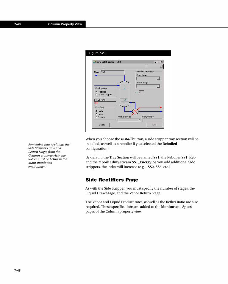
7-48 Column Property View
7-48
When you choose the Install button, a side stripper tray section will be installed, as well as a reboiler if you selected the Reboiled configuration.
By default, the Tray Section will be named SS1, the Reboiler SS1_Reb and the reboiler duty stream SS1_Energy. As you add additional Side strippers, the index will increase (e.g. - SS2, SS3, etc.).
Side Rectifiers Page
As with the Side Stripper, you must specify the number of stages, the Liquid Draw Stage, and the Vapor Return Stage.
The Vapor and Liquid Product rates, as well as the Reflux Ratio are also required. These specifications are added to the Monitor and Specs pages of the Column property view.
Figure 7.23
Remember that to change the Side Stripper Draw and Return Stages from the Column property view, the Solver must be Active in the Main simulation environment.
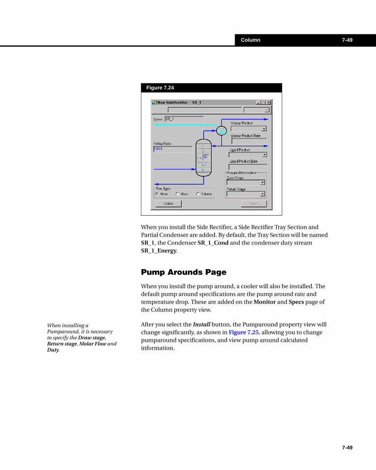
Column 7-49
When you install the Side Rectifier, a Side Rectifier Tray Section and Partial Condenser are added. By default, the Tray Section will be named SR_1, the Condenser SR_1_Cond and the condenser duty stream SR_1_Energy.
Pump Arounds Page
When you install the pump around, a cooler will also be installed. The default pump around specifications are the pump around rate and temperature drop. These are added on the Monitor and Specs page of the Column property view.
After you select the Install button, the Pumparound property view will change significantly, as shown in Figure 7.25, allowing you to change pumparound specifications, and view pump around calculated information.
Figure 7.24
When installing a Pumparound, it is necessary to specify the Draw stage, Return stage, Molar Flow and Duty.
7-49

7-50 Column Property View
7-50
Vap Bypasses Page
As with the Pumparound, it is necessary to specify the Draw and Return stage, as well as the Molar Flow and Duty for the Vapor Bypass. When you install the vapor bypass, the draw temperature and flowrate will be displayed on the Vapor Bypass view.
The Vapor Bypass flowrate is automatically added as a specification. Figure 7.26 shows the Vapor Bypass view once the side operation has been installed.
Figure 7.25
Figure 7.26

Column 7-51
Side Draws Page
The Side Draws page allows you to view and edit information regarding the side draw streams in the column. The information included on this page are: Draw Stream, Draw Stage, Type (Vapor, Liquid or Water), Mole Flow, Mass Flow and Volume Flow.
7.4.4 Rating TabThe Rating tab has four pages: the Tray Sections, Vessels, Equipment and Pressure Drop pages.
Page Description
Tray Sections
This page provides information regarding tray sizing. On this page, you can specify the following:
• Tray Section (Name)• Tray Diameter• Weir Height• Weir Length• Tray Space• Tray Volume
Vessels
This page provides information regarding vessel sizing. On this page, you can specify the following:
• Vessel (Name)• Diameter• Length• Volume• Orientation• Vessel has a Boot• Boot Diameter• Boot Length
Equipment This page contains a list of Other Equipment in the Column flowsheet.
Pressure Drop
This page contains information regarding pressure drop across the column. On this page you can specify the following information:
• Pressure Tolerance• Pressure Drop Tolerance• Damping Factor• Maximum Pressure Iterations• Top and Bottom column pressures
7-51

7-52 Column Property View
7-52
7.4.5 Worksheet TabThe Worksheet tab contains a summary of the information contained in the stream property view for all the streams attached to the unit operation. The Conditions, Properties, and Composition pages contain selected information from the corresponding pages of the Worksheet tab for the stream property view. The PF Specs page contains a summary of the stream property view’s Dynamics tab.
7.4.6 Performance TabOn the Performance tab, you can view the results of a converged column on the Summary page, the graphical and tabular presentation of the column profile on the Results page, and pinch information on the individual trays on the Pinch page.
Summary Page
The Summary Page gives a tabular summary of Column stage temperatures, pressures, flows and duties.
You may change the basis for which the data is displayed by selecting the appropriate radio button in the Flow Basis group. For the Feeds and Draw Streams, the VF column to the right of each flow value indicates whether the flow is vapor (V) or liquid (L). If the feed has been split, a star (*) will follow the phase designation. If there is a duty stream on a
Figure 7.27
Note that the Column Environment also has its own Workbook.
Note that the Liquid and vapor flows are net flows for each stage.
You can split a feed stream into its phase components either on the Connections page of the Design tab or on the Setup page on the Summary tab.

Column 7-53
stage, a "Q" will appear in the Type column to the right of the Feed Column. Note that the direction of the energy stream is indicated by the sign of the duty, rather than the column in which the "Q" appears. In the Type column, an “F” designates a feed stream and a “D” designates a draw stream.
Results Page
On the Results page, you can view various column profiles or refinery assay curves in a graphical or tabular format.
Tray by Tray Properties Group
To view a column profile, follow this generalized procedure:
1. Select a profile from the list in the Tray by Tray Properties group. The choices include: Temperature, Pressure, Flow, MW, Dens, Visc., Composition, K Value and Light/Heavy Key.
2. Specify the stage tray flow basis by selecting the appropriate radio button: Net or Total. Where the net basis only includes interstage flow and the total basis includes draw and pumparound flow.
Figure 7.28
7-53

7-54 Column Property View
7-54
3. In the Column Tray Ranges group, select the appropriate radio button:
4. After selecting a tray range, click either the View Graph or View Table button to display a plot or table respectively.
Depending on the profile selected, you may have to make further specifications. There is a Properties button on both the profile plot and table. By selecting this button, you will access the Properties view where you can customize the display of your profile. Changes made on the Properties view will affect both the table and plot. A description of the specifications available for each profile type is outlined in the following table.
Radio Button Action
All Displays the selected profile for all trays connected to the column (i.e. main tray section, side strippers, condenser, reboiler, etc.)
Single
From the drop down list, select a tray section. The main tray section along with the condenser and reboiler are considered one section, as is each side stripper.
From/To
Use the drop-down lists to specify a specific range of the column. The first cell will contain the tray that is located at a higher spot in the tower (i.e. for top to bottom tray numbering, the first cell could be tray 3 and the second tray 6).
To make changes to the plot, object Inspect the plot area and select Graph Control from the menu. Refer to Chapter 6 - Output Control in the User’s Guide.
Figure 7.29
Plots and tables are expandible views that can remain open without the column property view.
Profile Type Description
Temperature ProfileThe temperature profile displays the temperature for the tray range selected. No further specification is needed.
Pressure ProfileThe pressure profile displays the pressure of each tray in the selected range. No further specification is needed for this profile.

Column 7-55
Flow Profile
In the Basis group box, select Molar, Mass or Liquid Volume for your flow profile basis.
In the Phase group, activate the check box for the flow of each phase that you wish to display. Multiple flows can be shown. If three phases are not present in the column, the Heavy Liquid check box will not be available, and thus, the Light Liquid check box will represent the liquid phase.
Properties Profile (MW. Dens., Visc...)
In the Basis group box, select Molar, Mass or Liquid Volume for the properties profile basis.
In the Phase group box, activate the check box for the flow of each phase that you wish to display. Multiple flows can be shown. If three phases are not present in the column, the Heavy Liquid check box will not be available, as is the case in the above figure.
In the Axis Assignment group, by selecting a radio button under Left, you will assign the values of the appropriate property to the left y-axis. To display a second property, choose a radio button under Right. The right y-axis will then show the range of the second property. If you wish to display only one property on the plot, select the None radio button under Right.
Profile Type Description
The Properties Profile table displays all of the properties for the phase(s) selected.
7-55
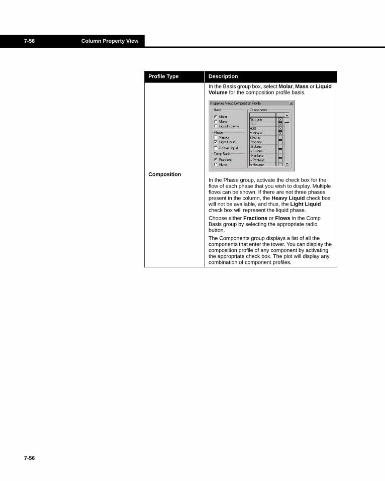
7-56 Column Property View
7-56
Composition
In the Basis group box, select Molar, Mass or Liquid Volume for the composition profile basis.
In the Phase group, activate the check box for the flow of each phase that you wish to display. Multiple flows can be shown. If there are not three phases present in the column, the Heavy Liquid check box will not be available, and thus, the Light Liquid check box will represent the liquid phase.
Choose either Fractions or Flows in the Comp Basis group by selecting the appropriate radio button.
The Components group displays a list of all the components that enter the tower. You can display the composition profile of any component by activating the appropriate check box. The plot will display any combination of component profiles.
Profile Type Description

Column 7-57
K Values Profile
The K Values profile displays the K Values of each tray in the selected range. From the Properties view you can select which components you want included in the profile.
Light/Heavy Key Profile
This profile displays the fraction ratio for each stage. In the Basis group box, select Molar, Mass or Liquid Volume for the profile basis.
In the Phase group, select Vapor, Light Liquid or Heavy Liquid, and in the Comp Basis group, select Fractions or Flows. In the Light Key(s) and Heavy Key(s) groups, you can select the key component(s) to include in your profile.
Profile Type Description
7-57
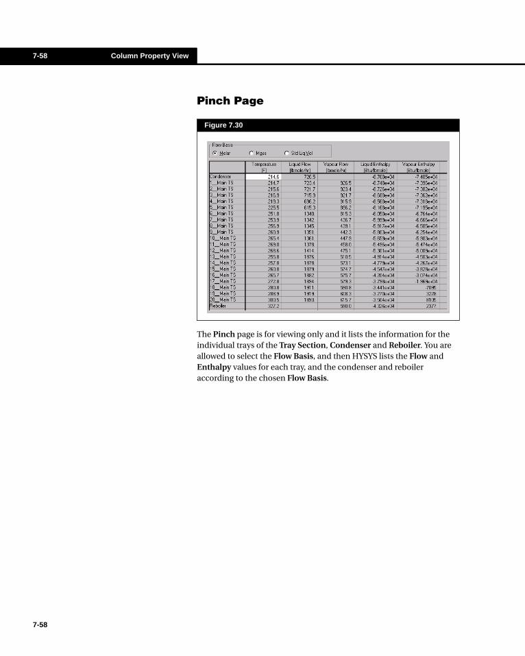
7-58 Column Property View
7-58
Pinch Page
The Pinch page is for viewing only and it lists the information for the individual trays of the Tray Section, Condenser and Reboiler. You are allowed to select the Flow Basis, and then HYSYS lists the Flow and Enthalpy values for each tray, and the condenser and reboiler according to the chosen Flow Basis.
Figure 7.30

Column 7-59
2/3 Phase Page
This 2/3 Phase Page on the Performance tab displays additional liquid flow rate information associated with three-phase distillation. You can specify that HYSYS check for and calculate the flowrate of a second liquid phase on any or all the trays of the column.This information is then displayed in the L2Rate column. The Summary page displays a single liquid flowrate for each stage of the column; you must view this page to see the two-liquid-phase breakdown of the liquid stream.
Note that the 2nd Liquid Type group lists two options: Rigorous and Pure. The Rigorous method can take substantially longer to solve than the Pure method. When dealing with hydrocarbons, the Pure method is the preferred choice. When dealing with chemicals (using activity models) the Rigorous method may produce better results.
Figure 7.31
By default, HYSYS will select Pure for all hydrocarbon and Rigorous for all chemical based distillations. This default selection criteria is based on the type of Fluid Package used but can always be changed by the user.
7-59
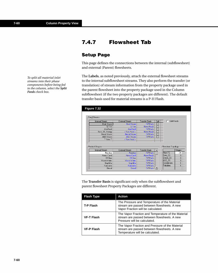
7-60 Column Property View
7-60
7.4.7 Flowsheet Tab
Setup Page
This page defines the connections between the internal (subflowsheet) and external (Parent) flowsheets.
The Labels, as noted previously, attach the external flowsheet streams to the internal subflowsheet streams. They also perform the transfer (or translation) of stream information from the property package used in the parent flowsheet into the property package used in the Column subflowsheet (if the two property packages are different). The default transfer basis used for material streams is a P-H Flash.
The Transfer Basis is significant only when the subflowsheet and parent flowsheet Property Packages are different.
Figure 7.32
To split all material inlet streams into their phase components before being fed to the column, select the Split Feeds check box.
Flash Type Action
T-P FlashThe Pressure and Temperature of the Material stream are passed between flowsheets. A new Vapor Fraction will be calculated.
VF-T FlashThe Vapor Fraction and Temperature of the Material stream are passed between flowsheets. A new Pressure will be calculated.
VF-P FlashThe Vapor Fraction and Pressure of the Material stream are passed between flowsheets. A new Temperature will be calculated.

Column 7-61
When the Split check box for any of the inlet material streams is selected, that stream is split into its vapor and liquid phase components when fed to the column. The liquid stream is then fed to the specified tray and the vapor phase to the tray immediately above the specified feed tray.
The Flowsheet Topology group provides stage information for each element in the flow sheet. In Figure 7.32, the Flowsheet Topology group shows the number of stages involved with the Main TS, Kero_SS, Diesel_SS, AGO_SS, Condensers, and Reboilers.
Flowsheet Variables Page (Main)
This page allows you to select and monitor any flowsheet variables from one location. You can examine subflowsheet variables from the outside Column property view, without actually having to enter the Column subflowsheet environment.
You can add, edit or delete variables in the Selected Column flowsheet Variables group.
Adding a Variable
1. Press the Add button.
2. From the Variable Navigator, select each of the parameters for the variable.
3. Press the OK button.
4. The variable is added to the Selected Column Flowsheet Variables group.
P-H FlashThe Pressure and Enthalpy of the Material stream is passed between flowsheets. This is the default transfer basis.
User Specs You specify the Transfer Basis for a Material Stream.
None Required No calculation is required for an Energy stream. The heat flow will simply be passed between flowsheets.
Flash Type Action
Figure 7.33
See the Summary page of the Performance tab to verify the split feed streams. An asterisk (*) following the phase indicator in the VF column indicates a split stream.
You can also use the Specifications page to view certain variables. Select the variable by adding a specification, and ensure that the Active and Estimate boxes are not checked. The value of this variable will be displayed in the Current value column, and this "pseudo-specification" will not affect the solution.
Refer to Section 5.2.2 - Variable Navigator in the User’s Guide for information on the Variable Navigator.
7-61

7-62 Column Property View
7-62
Editing a Variable
You can edit a variable in the Selected Column Flowsheet Variables group as follows:
1. Highlight a variable.
2. Press the Edit button.
3. Make changes to the selections in the variable navigator.
4. Press the OK button.
Deleting a Variable
You can remove a variable in any of the following ways:
• Highlight a variable and press the Delete button.• Highlight a variable, press the Edit button, and then press the
Disconnect button from the Variable Navigator.
Internal Streams Page
On this page, you can create a flowsheet stream that will represent any phase leaving any tray within the Column. Streams within operations attached to the main tray section (i.e. side strippers, the condenser, the reboiler, etc.) can also be targeted. Each time changes occur to the column, new information will automatically be transferred to the stream which you have created.
To demonstrate the addition of an internal stream, a stream representing the liquid phase flowing from tray 7 to tray 8 in the main tray section of a column is added:
1. Press the Add button.
2. Place the cursor in the cell under Stream and enter the name Liquid7. The name will appear in the edit bar as you type.
3. With the cursor in the cell under Stage, you can open the drop down list in the edit bar and choose tray 7 or simply type 7, which will locate the selection in the list.
Figure 7.34
If you decide that you do not want to keep the changes made in the variable navigator, press the Cancel button.

Column 7-63
4. Under Type, you can select the phase that you wish to represent. The options include Vapor, Liquid or Aqueous. Select Liquid in this case.
5. When the cursor is in the cell under Net/Total, you must select either Net or Total. Net represents the material flowing from the Stage you have selected to the next stage (above for vapor, below for liquid or aqueous) in the column. By selecting Total, the internal stream will represent all the material leaving the stage (i.e. includes draws, pumparound streams, etc.). For the stage 7 liquid, Net was selected.
7.4.8 Reactions TabReactive distillation has been used for many years to carry out chemical reactions, in particular esterification reactions. The advantages of using distillation columns for carrying out chemical reactions include:
• the possibility of driving the reaction to completion (break down of thermodynamic limitations for a reversible reaction) and separating the products of reactions in only one unit, thus eliminating recycle and reactor costs.
• the elimination of possible side reactions by continuous withdrawal of one of the products from the liquid phase.
• the operation at higher temperatures (boiling liquid) thus increasing the rate of reaction of endothermic reactions.
• the internal recovery of the heat of reaction for exothermic reactions, thereby replacing an equivalent amount of external heat input required for boil-up.
The Reactions tab allows you to attach multiple reactions to the column. The tab consists of two pages: the Stages page which allows you select the reaction set and its scope across the column and the Results page which displays the reaction results stage by stage.
Before adding a reaction to a column you must first ensure that you are using the correct column Solving Method. HYSYS provides three solving methods which allow for reactive distillation.
Solving Method Reaction Type Reaction Phase
Sparse Continuation Solver
Kinetic Rate, Simple Rate, Equilibrium Reaction
Vapor, Liquid
Newton Raphson Inside-Out
Kinetic Rate, Simple Rate
Liquid
Simultaneous CorrectionKinetic Rate, Simple Rate, Equilibrium Reaction
Vapor, Liquid, Combined Phase
7-63

7-64 Column Property View
7-64
Note also that the Sparse Continuation Solver method allows you to attach a reaction set to your column which combines reaction types. Other solvers require that the attached reactions are of a single type.
Stages Page
The Stages page consists of the Column Reaction Stages group. The group contains the Column Reaction Stages matrix and three buttons.
Column Reaction Stages Matrix
The matrix consists of four columns.
Figure 7.35
Column Description
Column Reaction Name
This is the name you have associated with column reaction. Note that this is not the name of the reaction set you set in the Fluid Package manager.
First Stage The highest stage of the stage range over which the reaction will be occurring.
Last Stage The lowest stage of the stage range over which the reaction will be occurring.
Active Activates the associated reaction thereby enabling it to occur inside the column.
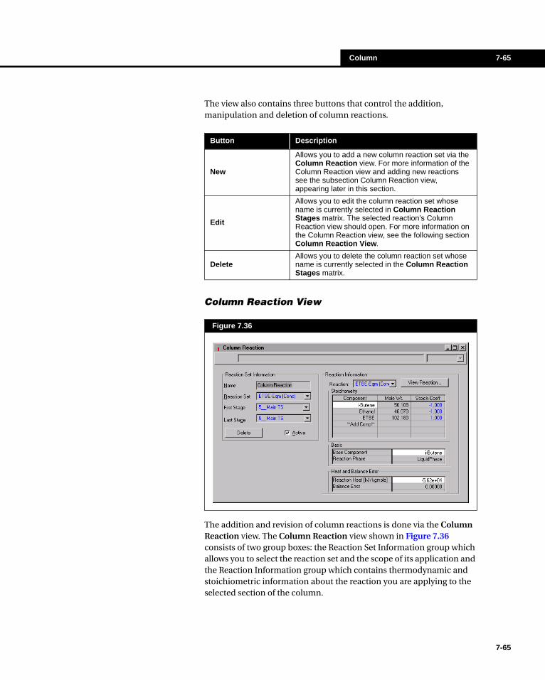
Column 7-65
The view also contains three buttons that control the addition, manipulation and deletion of column reactions.
Column Reaction View
The addition and revision of column reactions is done via the Column Reaction view. The Column Reaction view shown in Figure 7.36 consists of two group boxes: the Reaction Set Information group which allows you to select the reaction set and the scope of its application and the Reaction Information group which contains thermodynamic and stoichiometric information about the reaction you are applying to the selected section of the column.
Button Description
New
Allows you to add a new column reaction set via the Column Reaction view. For more information of the Column Reaction view and adding new reactions see the subsection Column Reaction view, appearing later in this section.
Edit
Allows you to edit the column reaction set whose name is currently selected in Column Reaction Stages matrix. The selected reaction’s Column Reaction view should open. For more information on the Column Reaction view, see the following section Column Reaction View.
DeleteAllows you to delete the column reaction set whose name is currently selected in the Column Reaction Stages matrix.
Figure 7.36
7-65
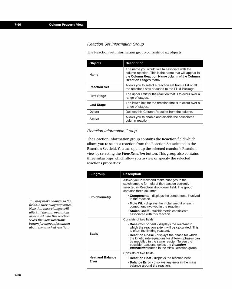
7-66 Column Property View
7-66
Reaction Set Information Group
The Reaction Set Information group consists of six objects:
Reaction Information Group
The Reaction Information group contains the Reaction field which allows you to select a reaction from the Reaction Set selected in the Reaction Set field. You can open up the selected reaction’s Reaction view by selecting the View Reaction button. This group also contains three subgroups which allow you to view or specify the selected reactions properties:
Objects Description
Name
The name you would like to associate with the column reaction. This is the name that will appear in the Column Reaction Name column of the Column Reaction Stages matrix.
Reaction Set Allows you to select a reaction set from a list of all the reactions sets attached to the Fluid Package.
First Stage The upper limit for the reaction that is to occur over a range of stages.
Last Stage The lower limit for the reaction that is to occur over a range of stages.
Delete Deletes this Column Reaction from the column.
Active Allows you to enable and disable the associated column reaction.
Subgroup Description
Stoichiometry
Allows you to view and make changes to the stoichiometric formula of the reaction currently selected in Reaction drop down field. The group contains three columns:
• Components - displays the components involved in the reaction.
• Mole Wt. - displays the molar weight of each component involved in the reaction.
• Stoich Coeff - stoichiometric coefficients associated with this reaction.
Basis
Consists of two fields:
• Base Component - displays the reactant to which the reaction extent will be calculated. This is often the limiting reactant.
• Reaction Phase - displays the phase for which the kinetic rate equations for different phases can be modelled in the same reactor. To see the possible reactions, select the Reaction Information button in the View Reaction group.
Heat and Balance Error
Consists of two fields:
• Reaction Heat - displays the reaction heat.• Balance Error - displays any error in the mass
balance around the reaction.
You may make changes to the fields in these subgroup boxes. Note that these changes will affect all the unit operations associated with this reaction. Select the View Reactions button for more information about the attached reaction.
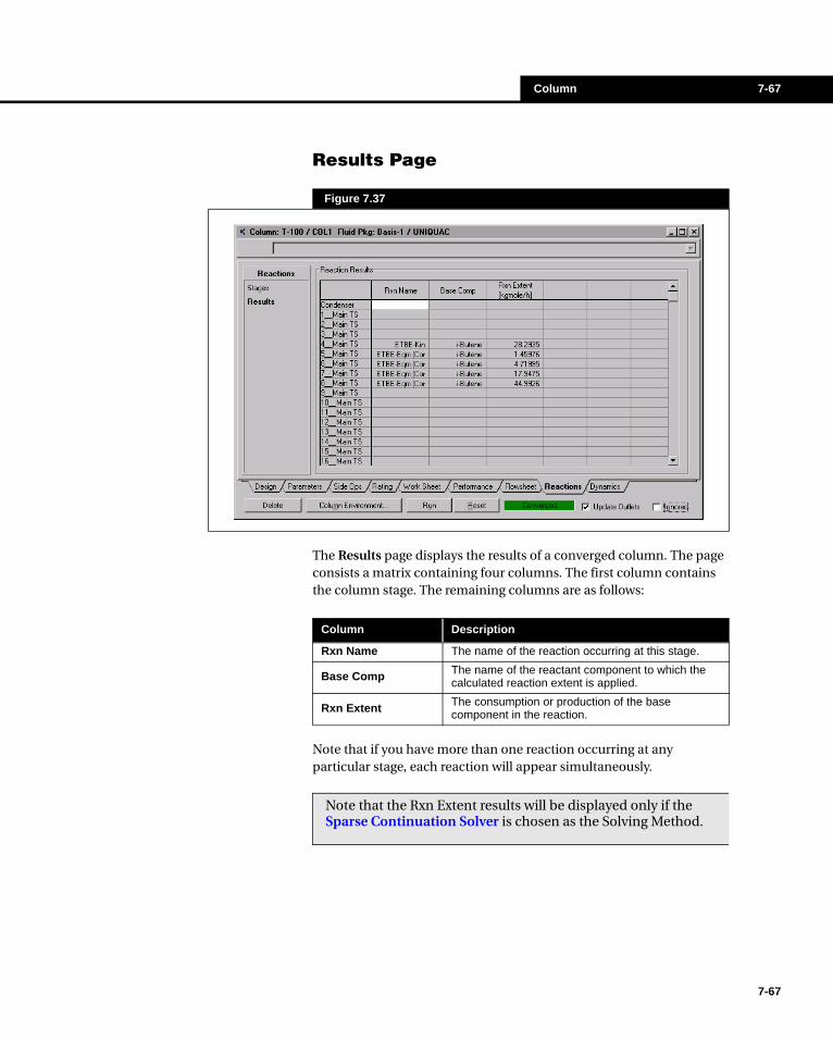
Column 7-67
Results Page
The Results page displays the results of a converged column. The page consists a matrix containing four columns. The first column contains the column stage. The remaining columns are as follows:
Note that if you have more than one reaction occurring at any particular stage, each reaction will appear simultaneously.
Figure 7.37
Column Description
Rxn Name The name of the reaction occurring at this stage.
Base Comp The name of the reactant component to which the calculated reaction extent is applied.
Rxn Extent The consumption or production of the base component in the reaction.
Note that the Rxn Extent results will be displayed only if the Sparse Continuation Solver is chosen as the Solving Method.
7-67

7-68 Column Property View
7-68
Design Tips for Reactive Distillation1Although the column unit operations allows for multiple column reactions and numerous column configurations, a general column topography can subdivided into three sections: the Rectifying Section, Reactive Section and the Stripping Section.
While the Rectifying and Stripping Sections are similar to ordinary distillation, a reactive distillation column also has a Reactive Section. The Reactive Section of the column is where the main reactions occur. There is no particular requirement for separation in this section.
There are several unique operational considerations when designing a reactive distillation column:
• The operating pressure should be predicated on the indirect effects of pressure on reaction equilibrium.
• The optimum feed point to a reactive distillation column is just below the reactive section. Introducing a feed too far below the reactive section reduces the stripping potential of the column and results in increased energy consumption.
• Reflux has a dual purpose in reactive distillation. Increasing the reflux rate enhances separation and recycles unreacted reactants to the reaction zone thereby increasing conversion.
Figure 7.38
Stripping Section
Reactive Section
Rectifying Section
Column 7-69
• Reboiler Duty is integral to reactive distillation as it must be set to ensure sufficient recycle of unreacted, heavy reactant to the reaction zone without excluding the light reactant from the reaction zone, if the reboiler duty is too high or too low, conversion and purity may be compromised.
7.4.9 Dynamics TabThe Dynamics tab has three related pages: Vessels, Equipment and Holdup. If you are working exclusively in Steady State mode or your version of HYSYS does not support dynamics, you are not required to change any information on the pages accessible through this tab. For more information on running the Column operation in Dynamic mode, see the Dynamic Modeling guide for further details.
7.5 Column Specification Types
This section outlines the various Column specification (spec) types available along with relevant details. Specs are added and modified on the Specs Page or the Monitor Page of the Design tab.
Adding and changing Column specifications is straightforward. If you have created a Column based on one of the templates, HYSYS already has default specifications in place. The type of default specification depends on which of the templates you have chosen (see the Default Replaceable Specifications sub section in Section 7.3.2 - Templates) for more details.
7-69
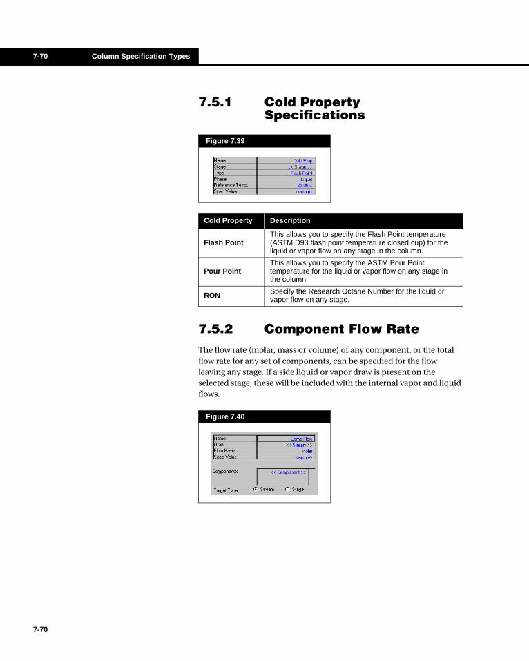
7-70 Column Specification Types
7-70
7.5.1 Cold Property Specifications
7.5.2 Component Flow RateThe flow rate (molar, mass or volume) of any component, or the total flow rate for any set of components, can be specified for the flow leaving any stage. If a side liquid or vapor draw is present on the selected stage, these will be included with the internal vapor and liquid flows.
Figure 7.39
Cold Property Description
Flash PointThis allows you to specify the Flash Point temperature (ASTM D93 flash point temperature closed cup) for the liquid or vapor flow on any stage in the column.
Pour PointThis allows you to specify the ASTM Pour Point temperature for the liquid or vapor flow on any stage in the column.
RON Specify the Research Octane Number for the liquid or vapor flow on any stage.
Figure 7.40

Column 7-71
7.5.3 Component FractionsThe mole, mass or volume fraction can be specified in the liquid or vapor phase for any stage. You can specify a value for any individual component, or specify a value for the sum of the mole fractions of multiple components.
7.5.4 Component RatioThe ratio (molar, mass or volume fraction) of any set of components over any other set of components can be specified for the liquid or vapor phase on any stage.
7.5.5 Component RecoveryThis is the molar, mass or volume flow of a component (or group of components) in any internal or product stream draw divided by the flow of that component (or group) in the combined tower feeds. As the recovery is a ratio between two flows, you specify a fractional value. Also, there is no need to specify a Flow Basis since this is a ratio of the same component between specified stream and the combined tower feeds.
Figure 7.41
Figure 7.42
7-71

7-72 Column Specification Types
7-72
7.5.6 Cut PointThis option allows a cutpoint temperature to be specified for the liquid or vapor leaving any stage. The types are TBP, ASTM D86, D1160 Vac, D1160 ATM, ASTM D2887. For D86, you will be given the option to use ASTM Cracking Factor. For D1160, you will be given an Atmospheric Pressure option. The cutpoint can be on a mole, mass or volume fraction basis, and any value from 0 to 100 percent is allowed.
7.5.7 Draw RateThe molar, mass or volume flowrate of any product stream draw may be specified.
7.5.8 Delta T (Heater/Cooler)The temperature difference across a heater or cooler unit operation may be specified. The heater/cooler unit must be installed in the Column subflowsheet and the Modified HYSIM Inside-Out Solving Method must be selected on the Solver page of the Parameters tab.
Figure 7.43
Figure 7.44
Figure 7.45
Note that while initial and final cutpoints are permitted, it is often better to use 5 and 95 percent cutpoints to minimize the errors introduced at the extreme ends of boiling point curves

Column 7-73
7-73
7.5.9 Delta T (Streams)The temperature difference between two Column subflowsheet streams may be specified.
7.5.10 DutyYou can specify the duty for an energy stream.
7.5.11 Duty RatioYou may specify the duty ratio for any two energy streams. In addition to Column feed duties, the choice of energy streams also includes Pump Around duties (if available).
7.5.12 Feed RatioSelecting this allows you to establish a ratio between the flow rate on or from any stage in the column and the external feed to a stage. You will be prompted for the stage, flow type (Vapor, Liquid, Draw), and the external feed stage.
Figure 7.46
Figure 7.47
Figure 7.48
Figure 7.49
This type of specification is useful for turn down or overflash of a crude feed.
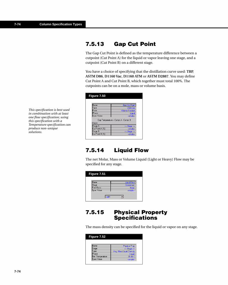
7-74 Column Specification Types
7-74
7.5.13 Gap Cut PointThe Gap Cut Point is defined as the temperature difference between a cutpoint (Cut Point A) for the liquid or vapor leaving one stage, and a cutpoint (Cut Point B) on a different stage.
You have a choice of specifying that the distillation curve used: TBP, ASTM D86, D1160 Vac, D1160 ATM or ASTM D2887. You may define Cut Point A and Cut Point B, which together must total 100%. The cutpoints can be on a mole, mass or volume basis.
7.5.14 Liquid FlowThe net Molar, Mass or Volume Liquid (Light or Heavy) Flow may be specified for any stage.
7.5.15 Physical Property Specifications
The mass density can be specified for the liquid or vapor on any stage.
Figure 7.50
Figure 7.51
Figure 7.52
This specification is best used in combination with at least one flow specification; using this specification with a Temperature specification can produce non-unique solutions.

Column 7-75
7.5.16 Pump Around Specifications
7.5.17 Reboil RatioSpecifies the molar, mass or volume ratio of the vapor leaving a specific stage to the liquid leaving that stage.
Specification Description
Flow Rate The flow rate of the Pump Around can be specified in molar, mass or liquid volume units.
Temperature Drop
This option allows you to specify the temperature drop across a Pump Around exchanger. The conditions for using this specification are the same as that stated for Pump Around return temperature.
Return Temperature
The return temperature of a Pump Around stream can be specified. Ensure that you have not also specified both the pump around rate and the duty. This would result in the three associated variables (flow rate, side exchanger duty, and temperature) all specified, leaving HYSYS with nothing to vary in search of a converged solution.
Duty You may specify the duty for any Pump Around.
Return Vapor Fraction
You may specify the return vapor fraction for any Pump Around.
Duty Ratio
To specify a Pump Around duty ratio for a Column specification, add a Column Duty Ratio spec instead and select the Pump Around energy streams to define the duty ratio. Refer to Section 7.5.11 - Duty Ratio specification for further details.
Note that the Pump Around Rate as well as the Pump Around Temperature Drop are the default specifications HYSYS will request when a pump around is added to the column.
Figure 7.53
Figure 7.54
7-75

7-76 Column Specification Types
7-76
7.5.18 Reflux RatioThis is the molar, mass or volume flow of liquid (Light or Heavy) leaving a stage, divided by the sum of the vapor flow from the stage plus any side liquid flow.
7.5.19 Tee Split FractionThe split fraction for a TEE operation product stream can be specified. The TEE must be installed within the Column subflowsheet and directly attached to the column i.e. to a draw stream, in a pump around circuit, etc. Also, the Modified HYSIM Inside-Out Solving Method must be selected on the Params page.
Tee split fraction specifications are automatically installed as you install the tee operation in the Column subflowsheet; however, you can select which specifications become active on the Monitor or Specs page. Changes made to the split fraction specification value are updated on the Splits page of the tee operation.
7.5.20 Tray Temperature The temperature of any stage can be specified.
Figure 7.55
Figure 7.56
The Reflux Ratio specification is normally used only for top stage condensers, but it may be specified for any stage.
Refer to Section 4.3 - Tee for details on the TEE operation.
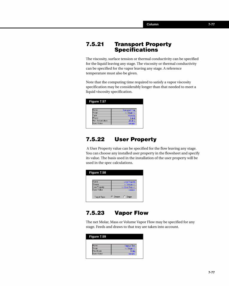
Column 7-77
7.5.21 Transport Property Specifications
The viscosity, surface tension or thermal conductivity can be specified for the liquid leaving any stage. The viscosity or thermal conductivity can be specified for the vapor leaving any stage. A reference temperature must also be given.
Note that the computing time required to satisfy a vapor viscosity specification may be considerably longer than that needed to meet a liquid viscosity specification.
7.5.22 User Property A User Property value can be specified for the flow leaving any stage. You can choose any installed user property in the flowsheet and specify its value. The basis used in the installation of the user property will be used in the spec calculations.
7.5.23 Vapor FlowThe net Molar, Mass or Volume Vapor Flow may be specified for any stage. Feeds and draws to that tray are taken into account.
Figure 7.57
Figure 7.58
Figure 7.59
7-77

7-78 Column Specification Types
7-78
7.5.24 Vapor FractionThe vapor fraction of a stream exiting a stage can be specified.
7.5.25 Vapor Pressure Specifications
Two types of vapor pressure specifications are available: true vapor pressure (@100°F) and Reid vapor pressure.
7.5.26 Column Stream Specifications
Column stream specifications must be created in the Column subflowsheet. Unlike other specifications, the stream specification is created through the stream’s property view, and not the Column Runner Specs page. To be able to add a specification to a stream:
• The Modified HYSIM Inside-out solving method must be chosen for the solver.
• The stream must be a draw stream.
The Create Column Stream Spec button on the Conditions page of the Worksheet tab is available only on Stream Property Views within the
Figure 7.60
Vapor Type Description
Vapor Pressure The true vapor pressure at 100°F can be specified for the vapor or liquid leaving any stage.
Reid Vapor Pressure
Reid vapor pressure can be specified for the vapor or liquid leaving any stage. The specification must always be given in absolute pressure units.
Figure 7.61
Only one stream specification may be created per draw stream.
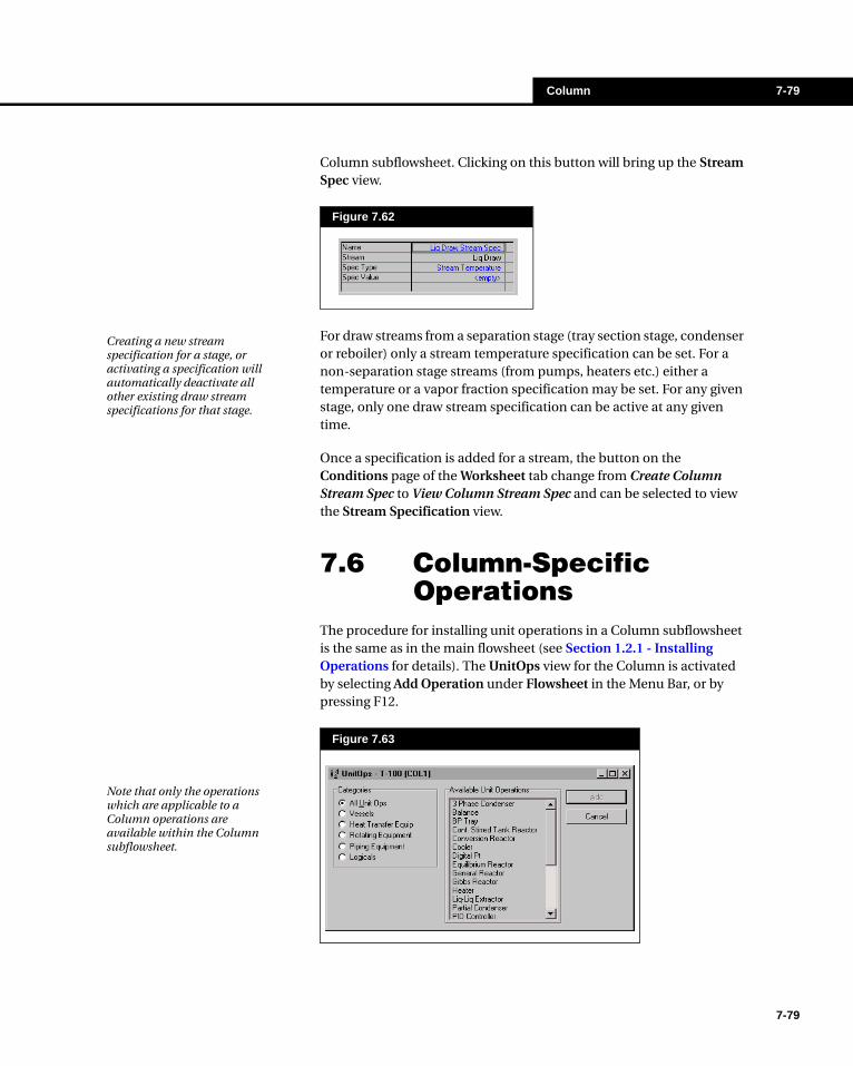
Column 7-79
Column subflowsheet. Clicking on this button will bring up the Stream Spec view.
For draw streams from a separation stage (tray section stage, condenser or reboiler) only a stream temperature specification can be set. For a non-separation stage streams (from pumps, heaters etc.) either a temperature or a vapor fraction specification may be set. For any given stage, only one draw stream specification can be active at any given time.
Once a specification is added for a stream, the button on the Conditions page of the Worksheet tab change from Create Column Stream Spec to View Column Stream Spec and can be selected to view the Stream Specification view.
7.6 Column-Specific Operations
The procedure for installing unit operations in a Column subflowsheet is the same as in the main flowsheet (see Section 1.2.1 - Installing Operations for details). The UnitOps view for the Column is activated by selecting Add Operation under Flowsheet in the Menu Bar, or by pressing F12.
Figure 7.62
Figure 7.63
Creating a new stream specification for a stage, or activating a specification will automatically deactivate all other existing draw stream specifications for that stage.
Note that only the operations which are applicable to a Column operations are available within the Column subflowsheet.
7-79

7-80 Column-Specific Operations
7-80
The unit operations available within the Column subflowsheet are listed in the following table. Most operations shown here are identical to those available in the main flowsheet in terms of supplied and calculated information, property view structure, etc.
There are also additional unit operations which are not available in the main flowsheet. They are: the Condenser (Partial, Total, 3-Phase), Reboiler and Tray Section. The Bypasses and Side Operations (Side Strippers, Pump Arounds, etc.) are available on the Side Ops page of the Column property view. Available unit operations in the Column subflowsheet are:
7.6.1 CondenserThe CONDENSER is used to condense vapor by removing its latent heat with a coolant. In HYSYS, the CONDENSER is used only in the Column Environment, and is generally associated with a Column TRAY SECTION.
There are four types of Condensers:
The Condenser property view uses a Type drop-down menu, letting you to switch between condenser types without having to delete and re-install a new piece of equipment.
Operation Category Types
Vessels3-Phase Condenser, Partial Condenser, Reboiler, Separator, Total Condenser, Tray Section
Heat Transfer Equipment Cooler, Heater, Heat Exchanger
Rotating Equipment Pump
Piping Equipment Valve
Logicals Balance, Digital Pt, PID Controller, Selector Block, Transfer Function Block
Condenser Type Description
Partial
Feed is partially condensed; there are vapor and liquid product streams. Note that the Partial Condenser can be operated as a total condenser by specifying the vapor stream to have zero flowrate.
Total Feed is completely condensed; there is a liquid product only.
Three-Phase - Chemical
There are two liquid product streams and one vapor product stream.
Three-Phase - Hydrocarbon
There is a liquid product streams and a water product stream and one vapor product stream.
Note that the PARTIAL CONDENSER can be used as a Total Condenser simply by specifying the vapor flowrate to be zero.

Column 7-81
When you switch between the condenser types, the pages will change appropriately. For instance, the Connections page for the TOTAL CONDENSER will not show the Vapor stream. If you switch from the PARTIAL to TOTAL CONDENSER, the Vapor stream is disconnected. If you then switch back, you will have to reconnect the stream.
When you add a Column to the simulation using a pre-defined template, there may be a CONDENSER attached to the tower (this is the case for a Distillation Column, for example). To manually add a Condenser, press F12 and make the appropriate selection from the UnitOps view or select a Condenser from the Column Palette.
The Condenser property view has the same basic five tabs that are available on any unit operation: Design, Rating, Worksheet, Performance and Dynamics.
It is necessary to specify the Connections and the Parameters for the Condenser. The information on the Rating and Dynamics tabs are not relevant in Steady State.
Figure 7.64
Partial Condenser Button
Total Condenser Button
Three-Phase Condenser Button
You are not required to modify information on the Condenser’s Rating or Dynamics tabs when working in Steady State Mode.
For a detailed description of the Rating and Dynamics tabs for the Condenser see Chapter 8 of the Dynamics Modelling guide for further information.
7-81

7-82 Column-Specific Operations
7-82
Design Tab
Connections Page
On the Connections page, provide the operation name, as well as the names of the Feed(s), Vapor, Water, Reflux, Product and Energy streams. The Total Condenser will not have a vapor stream, as the entire feed will be liquefied. Neither the Partial nor the Total Condenser has a Water Stream. The Connections page will show only the product streams which are appropriate for the selected condenser.
The Condenser is typically used with a tray section, where the vapor from the top tray of the column is the feed to the condenser, and the reflux from the condenser is returned to the top tray of the column.
Parameters Page
The condenser parameters that can be specified are:
• Pressure Drop• Duty• Subcooling Data
Figure 7.65
It is better to use a Duty spec than specifying the heat flow of the Duty stream.
Column 7-83
Pressure Drop
The Pressure Drop across the condenser (Delta P) is zero by default. It is defined in the following expression:
where:
P = Vessel pressure
Pv = Pressure of vapor product stream
Pl = Pressure of liquid product stream
Pfeed = Pressure of feed stream to Condenser
∆P = Pressure drop in vessel (Delta P)
Note that you typically supply a pressure for the condenser during the column setup, in which case the pressure of the top stage is the calculated value.
Duty
The Duty for the Energy stream can be specified here, but this is better done as a column spec (defined on the Monitor or Specs page of the Column property view). This allows for more flexibility when adjusting specifications, and also introduces a tolerance.
The Duty should be positive, indicating that energy is being removed from the Condenser feed. If the Energy stream was given a name on the Connections page, that name will be shown here.
The steady-state condenser energy balance is defined as:
where:
Hfeed = Heat flow of the feed stream to the Condenser
Hvapor = Heat flow of the vapor product stream
Hliquid = Heat flow of the liquid product stream(s)
(4.1)P Pv Pl Pfeed ∆P–= = =
If you specify the duty, it is equivalent to installing a duty spec, and a degree of freedom is used.
Hfeed - Duty = Hvapor + Hliquid (7.2)
7-83
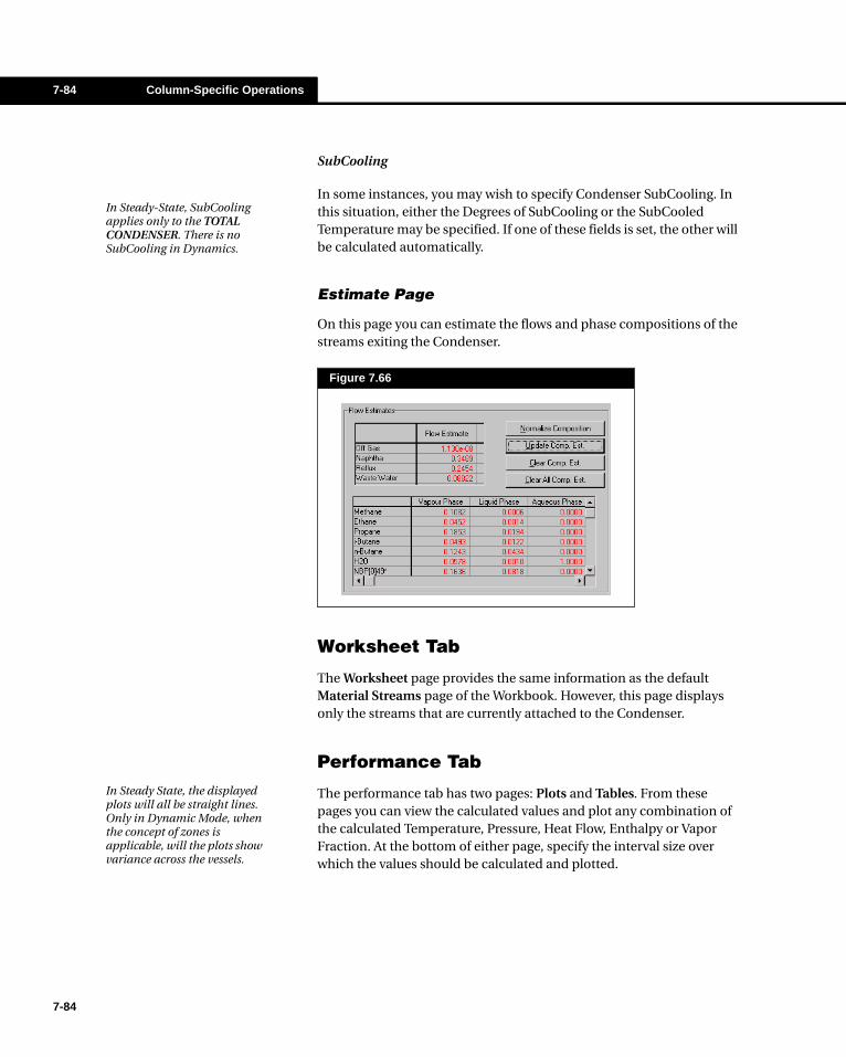
7-84 Column-Specific Operations
7-84
SubCooling
In some instances, you may wish to specify Condenser SubCooling. In this situation, either the Degrees of SubCooling or the SubCooled Temperature may be specified. If one of these fields is set, the other will be calculated automatically.
Estimate Page
On this page you can estimate the flows and phase compositions of the streams exiting the Condenser.
Worksheet Tab
The Worksheet page provides the same information as the default Material Streams page of the Workbook. However, this page displays only the streams that are currently attached to the Condenser.
Performance Tab
The performance tab has two pages: Plots and Tables. From these pages you can view the calculated values and plot any combination of the calculated Temperature, Pressure, Heat Flow, Enthalpy or Vapor Fraction. At the bottom of either page, specify the interval size over which the values should be calculated and plotted.
Figure 7.66
In Steady-State, SubCooling applies only to the TOTAL CONDENSER. There is no SubCooling in Dynamics.
In Steady State, the displayed plots will all be straight lines. Only in Dynamic Mode, when the concept of zones is applicable, will the plots show variance across the vessels.
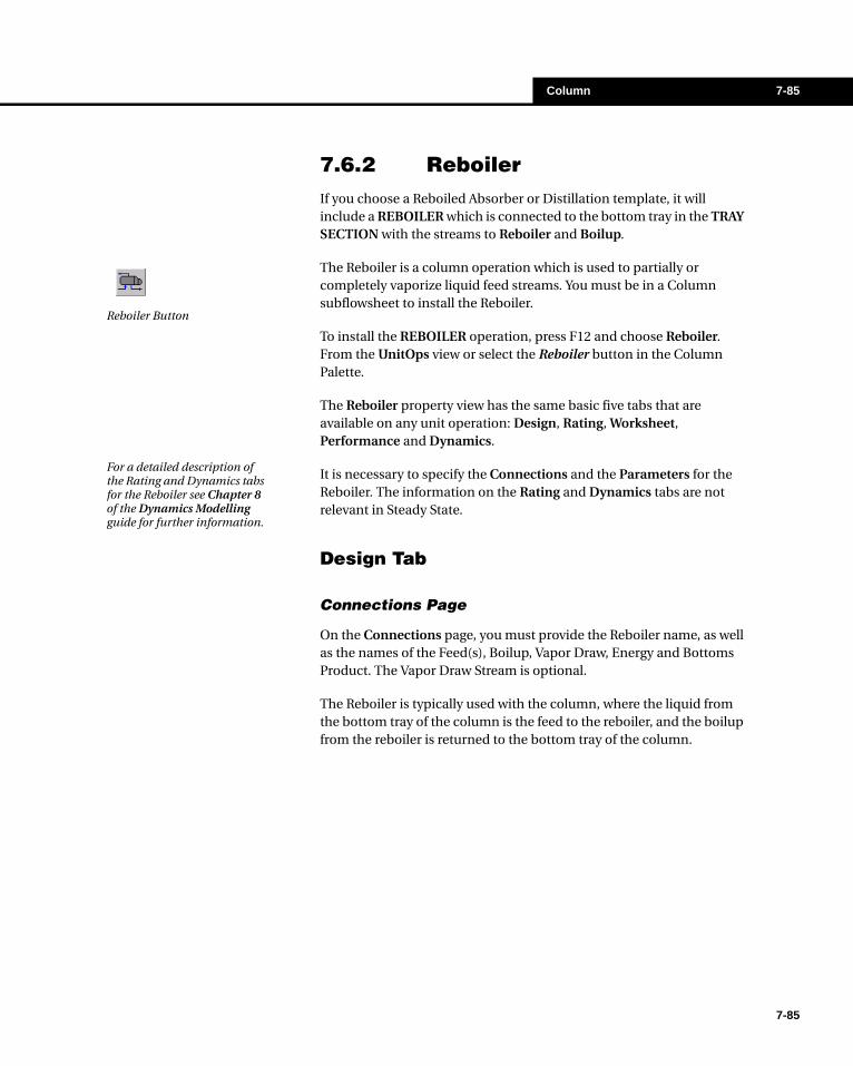
Column 7-85
7.6.2 ReboilerIf you choose a Reboiled Absorber or Distillation template, it will include a REBOILER which is connected to the bottom tray in the TRAY SECTION with the streams to Reboiler and Boilup.
The Reboiler is a column operation which is used to partially or completely vaporize liquid feed streams. You must be in a Column subflowsheet to install the Reboiler.
To install the REBOILER operation, press F12 and choose Reboiler. From the UnitOps view or select the Reboiler button in the Column Palette.
The Reboiler property view has the same basic five tabs that are available on any unit operation: Design, Rating, Worksheet, Performance and Dynamics.
It is necessary to specify the Connections and the Parameters for the Reboiler. The information on the Rating and Dynamics tabs are not relevant in Steady State.
Design Tab
Connections Page
On the Connections page, you must provide the Reboiler name, as well as the names of the Feed(s), Boilup, Vapor Draw, Energy and Bottoms Product. The Vapor Draw Stream is optional.
The Reboiler is typically used with the column, where the liquid from the bottom tray of the column is the feed to the reboiler, and the boilup from the reboiler is returned to the bottom tray of the column.
Reboiler Button
For a detailed description of the Rating and Dynamics tabs for the Reboiler see Chapter 8 of the Dynamics Modelling guide for further information.
7-85
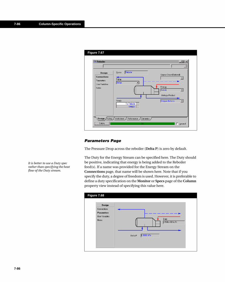
7-86 Column-Specific Operations
7-86
Parameters Page
The Pressure Drop across the reboiler (Delta P) is zero by default.
The Duty for the Energy Stream can be specified here. The Duty should be positive, indicating that energy is being added to the Reboiler feed(s). If a name was provided for the Energy Stream on the Connections page, that name will be shown here. Note that if you specify the duty, a degree of freedom is used. However, it is preferable to define a duty specification on the Monitor or Specs page of the Column property view instead of specifying this value here.
Figure 7.67
Figure 7.68
It is better to use a Duty spec rather than specifying the heat flow of the Duty stream.

Column 7-87
The steady-state reboiler energy balance is defined as:
where:
Hfeed = Heat flow of the feed stream to the Reboiler
Hvapor = Heat flow of the vapor draw stream
Hbottoms = Heat flow of the bottoms product stream
Hboilup = Heat flow of the boilup stream
Worksheet Tab
The Worksheet tab provides the same information as the default Material Streams page of the Workbook. However, this page displays only the streams that are currently attached to the Reboiler.
Performance Tab
The Performance tab has two pages: Plots and Tables. At the bottom of either page, specify the interval size over which the values should be calculated and plotted.
7.6.3 Tray SectionAt the very minimum, the Column Templates will include a TRAY SECTION. An individual tray has a vapor feed from the tray below, a liquid feed from the tray above and any additional feed, draw or duty streams to or from that particular tray.
Shown in Figure 7.69 is the property view for the TRAY SECTION of a Distillation Column template.
Hfeed + Duty = Hvapor + Hbottom + Hboilup (7.3)
7-87

7-88 Column-Specific Operations
7-88
The tray section property view contains the five tabs that are common to most unit operations: Design, Rating, Worksheet, Performance and Dynamics. You are not required to change anything on the Rating and Dynamics tabs because the information on these pages are not relevant in Steady State Mode.
Design Tab
Connections Page
The Connections page of the Tray Section is used for specifying the names and locations of vapor and liquid inlet and outlet streams, feed streams and the number of stages (see Figure 7.69). When a Column template is selected, HYSYS inserts the default stream names associated with the template into the appropriate input cells. For example, in a distillation column, the Tray Section vapor outlet stream is To Condenser and the Liquid inlet stream is Reflux.
A number of conventions exist for the naming and locating of streams associated with a Column TRAY SECTION:
• When you select a Tray Section feed stream, HYSYS by default feeds the stream to the middle tray of the column (for example, in a 20-tray column, the feed would enter on tray 10).
Figure 7.69
For more information on the dynamics of the tray section see Chapter 8 of the Dynamic Modelling guide.

Column 7-89
The location may be changed by selecting the desired feed tray from the Edit Bar drop-down list, or by entering the tray number in the appropriate field.
• Streams entering and leaving the top and bottom trays are always placed in the Liquid or Vapor Inlet/Outlet cells.
Side Draws Page
On the Side Draws page, specify the name and type of side draws taken from the tray section of your column. Use the radio buttons to select the type of side draw: Vapor, Liquid or Water and then the cells to name the side draw stream and specify the tray from which it is taken.
Parameters Page
You may input the number of trays on the Parameters page. The trays are treated as ideal if the fractional efficiencies are set to 1. If the efficiency of a particular tray is less than 1, the tray is modelled using a modified Murphree Efficiency.
Figure 7.70
Specifying the location of a column feed stream to be either the top tray (tray 1 or tray N, depending on your selected numbering convention) or the bottom tray (N or 1) will automatically result in the stream becoming the Liquid Inlet or the Vapor Inlet, respectively. If the Liquid Inlet or Vapor Inlet already exists, your specified feed stream will be an additional stream entering on the top or bottom tray, displayed with the tray number (1 or N). A similar convention exists for the top and bottom tray outlet streams (Vapor Outlet and Liquid Outlet).
By default, the Use Tray Section Name for Stage Name check box is selected.
7-89

7-90 Column-Specific Operations
7-90
You can add or delete trays anywhere in the column by selecting the Customize button and entering the appropriate information in the Custom Modify Number of Trays group. This feature makes adding and removing trays simple, especially if you have a complex column and you do not want to lose any feed or product stream information. Figure 7.71 shows the dialog box that appears when the Customize button is selected:
You may add and remove trays in the following ways:
• Specify a new number of trays in the Current Number of Trays cell. This is the same as changing the number of theoretical trays on the Connections page. All inlet and outlet streams will move appropriately; for example, if you are changing the number of trays from 10 to 20, a stream initially connected to tray 5 will now be at tray 10, and a stream initially connected at stream 10 will now be at tray 20.
To add trays to the tray section:
1. Enter the number of trays you wish to add in the Number of Trays to Add/Delete input cell.
2. Specify the tray number after which you wish to add the trays in the Tray to Add After or Delete First input cell.
3. Select the Add Trays button and HYSYS will insert the trays in the appropriate place according to the tray numbering sequence you are using. All streams (except feeds) and auxiliary equipment below (or above, depending on the tray numbering scheme) the tray where you inserted will be moved down (or up) by the number of trays that were inserted.
To remove trays from the tray section:
1. Enter the number of trays you wish to delete in the Number of Trays to Add/Delete input cell.
2. Enter the first tray in the section you wish to delete in the Tray to Add After or Delete First cell.
Figure 7.71
When you are adding or deleting trays, all FEEDS will remain connected to their current trays.
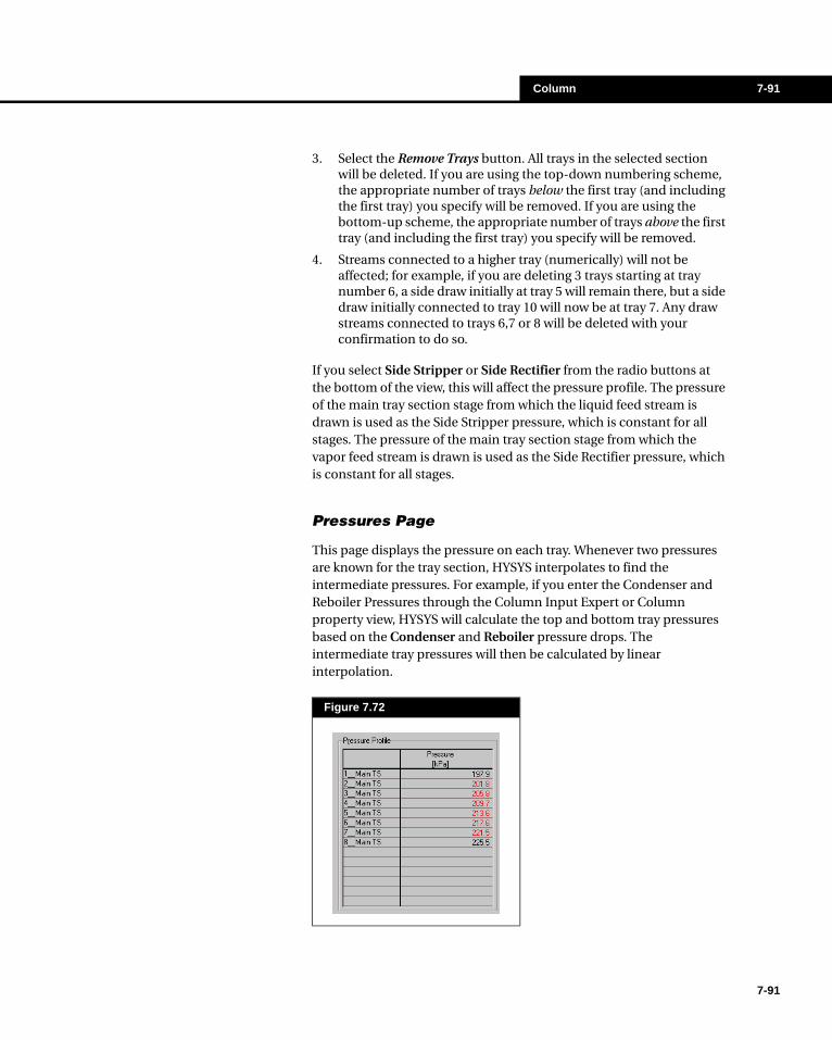
Column 7-91
3. Select the Remove Trays button. All trays in the selected section will be deleted. If you are using the top-down numbering scheme, the appropriate number of trays below the first tray (and including the first tray) you specify will be removed. If you are using the bottom-up scheme, the appropriate number of trays above the first tray (and including the first tray) you specify will be removed.
4. Streams connected to a higher tray (numerically) will not be affected; for example, if you are deleting 3 trays starting at tray number 6, a side draw initially at tray 5 will remain there, but a side draw initially connected to tray 10 will now be at tray 7. Any draw streams connected to trays 6,7 or 8 will be deleted with your confirmation to do so.
If you select Side Stripper or Side Rectifier from the radio buttons at the bottom of the view, this will affect the pressure profile. The pressure of the main tray section stage from which the liquid feed stream is drawn is used as the Side Stripper pressure, which is constant for all stages. The pressure of the main tray section stage from which the vapor feed stream is drawn is used as the Side Rectifier pressure, which is constant for all stages.
Pressures Page
This page displays the pressure on each tray. Whenever two pressures are known for the tray section, HYSYS interpolates to find the intermediate pressures. For example, if you enter the Condenser and Reboiler Pressures through the Column Input Expert or Column property view, HYSYS will calculate the top and bottom tray pressures based on the Condenser and Reboiler pressure drops. The intermediate tray pressures will then be calculated by linear interpolation.
Figure 7.72
7-91

7-92 Column-Specific Operations
7-92
Rating Tab
For information on the Rating tab refer to Section 8.4 - Tray Section in the Dynamics Modeling book.
Worksheet Tab
The Work Sheet tab provides the same information as the default Material Streams page of the Workbook. However, this page displays only the streams that are currently attached to the Tray Section.
Performance Tab
The Performance tab has two pages: Plots and Tables. At the bottom of either page, specify the interval size over which the values should be calculated and plotted.
Dynamic Tab
For more information on the Dynamic tab refer to Section 8.4 - Tray Section in the Dynamics Modeling book.
7.6.4 TeeThe TEE operation is available when using the Modified HYSIM I/O method only. The property view for the TEE operation in the Column subflowsheet has all of the pages and inherent functionality contained by the Tee in the Main Environment with one addition, the Estimates page.
Figure 7.73
Refer to Chapter 4 - Piping Equipment for more details on the property view of the TEE.
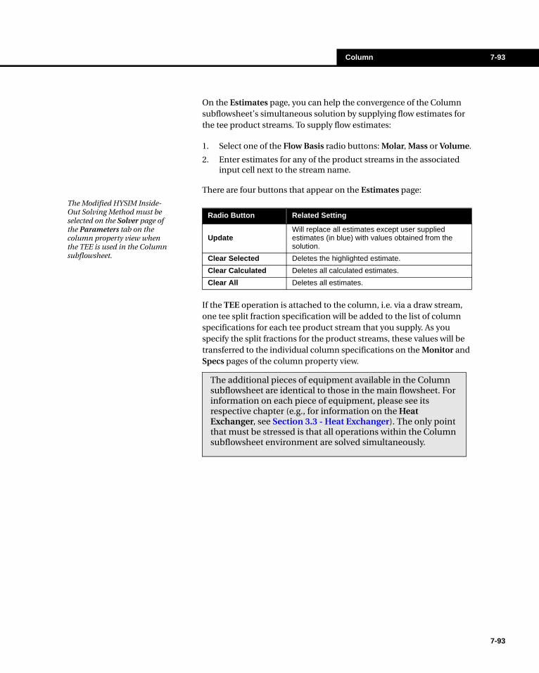
Column 7-93
On the Estimates page, you can help the convergence of the Column subflowsheet’s simultaneous solution by supplying flow estimates for the tee product streams. To supply flow estimates:
1. Select one of the Flow Basis radio buttons: Molar, Mass or Volume.
2. Enter estimates for any of the product streams in the associated input cell next to the stream name.
There are four buttons that appear on the Estimates page:
If the TEE operation is attached to the column, i.e. via a draw stream, one tee split fraction specification will be added to the list of column specifications for each tee product stream that you supply. As you specify the split fractions for the product streams, these values will be transferred to the individual column specifications on the Monitor and Specs pages of the column property view.
The Modified HYSIM Inside-Out Solving Method must be selected on the Solver page of the Parameters tab on the column property view when the TEE is used in the Column subflowsheet.
Radio Button Related Setting
UpdateWill replace all estimates except user supplied estimates (in blue) with values obtained from the solution.
Clear Selected Deletes the highlighted estimate.
Clear Calculated Deletes all calculated estimates.
Clear All Deletes all estimates.
The additional pieces of equipment available in the Column subflowsheet are identical to those in the main flowsheet. For information on each piece of equipment, please see its respective chapter (e.g., for information on the Heat Exchanger, see Section 3.3 - Heat Exchanger). The only point that must be stressed is that all operations within the Column subflowsheet environment are solved simultaneously.
7-93

7-94 Running the Column
7-94
7.7 Running the ColumnOnce you are satisfied with the configuration of your Column subflowsheet and you have supplied all necessary input, the next step is to run the Column solution algorithm.
The iterative procedure will begin when you select Run from the Column property view. Note that the Run/Reset buttons may be accessed from any page of the Column property view. When you are inside the Column build environment, a Run button also appears on the toolbar, which has the same function as the Run button on the Column property view.
When the Run button on the Column property view is selected, the Run/Reset buttons will be replaced by a Stop button which, when selected, will terminate the convergence procedure. The Run button may then be selected again to continue from the same location. Similarly, a Stop button replaces the toolbar Run button after it is activated.
When you are working inside the Column build environment, the Column will run only when you select the Run button on the Column property view, or the Run button from the button bar. When you are working with the Column property view in the Main build environment, the Column will automatically Run when:
• you change a specification value after a converged solution has been reached.
• you change the Active specifications, such that the Degrees of Freedom return to zero.
7.7.1 RunSelecting Run will begin the iterative calculations necessary to simulate the column described by the input. On the Monitor page of the Column property view, a summary showing the iteration number, equilibrium error, and the heat and specification errors will appear. Detailed messages showing the convergence status will be shown in the Trace Window (see Section 7.4.1 - Design Tab).
The default basis for the calculation is a modified "inside-out" algorithm. In this type of solution, simple equilibrium and enthalpy models are used in the inner loop which solve the overall component and heat balances, vapor-liquid equilibrium, and any specifications. The outer loop updates the simple thermodynamic models with rigorous calculations.
Run and Reset Buttons in the Columnproperty view.
Stop Button in the Column property view
Run Button (green) in the Button Bar
Stop Button (red) in the Button Bar
On the Button Bar, the Run and Stop buttons are two separate buttons. Whichever button is toggled on has light grey shading.

Column 7-95
When the simulation is run, the status line at the bottom of the screen will first track the calculation of the initial properties used to generate the simple models. Then the determination of a Jacobian matrix will be displayed, which is used in the solution of the inner loop. Next, the status line will report the inner loop errors and the relative size of the step taken on each of the inner loop iterations. Finally, the rigorous thermodynamics will again be calculated and the resulting equilibrium, heat and spec errors reported. The calculation of the inner loop and the outer loop properties continues until convergence is achieved, or you determine that the column will not converge and press Stop to terminate the calculation.
If difficulty is encountered in converging the inner loop, the program will occasionally recalculate the inner loop Jacobian. If no obvious improvement is being made with the printed equilibrium and heat and spec errors, press Stop to terminate the calculations and examine the available information for clues (see Section 7.8 - Column Troubleshooting) if trouble is encountered achieving the desired solution).
Any estimates which are displayed in the Column Profile and Estimates pages will be used as initial guesses for the convergence algorithm. If no estimates are present, HYSYS will begin the convergence procedure by generating initial estimates (see Section 7.4.2 - Parameters Tab for more information on the Estimates page).
7.7.2 ResetThis command will clear the current Column solution and any estimates appearing on the Estimates page of the Column view. If you make major changes after getting a converged Column, it may be a good idea to Reset to clear the previous solution. This will allow the Column solver to start fresh and distance itself from the previous solution. If you make only minor changes to the Column, try selecting Run before Resetting.
Once the column calculation is started it will continue until it has either converged, has been terminated due to a mathematically impossible condition, (e.g., being unable to invert the Jacobian matrix), or it has reached the maximum number of iterations. Other than these three situations, calculations will continue indefinitely in an attempt to solve the column unless the Stop button is selected. Unconverged results can be analysed, as discussed in Section 7.8 - Column Troubleshooting.
7-95

7-96 Column Troubleshooting
7-96
7.8 Column Troubleshooting
Although HYSYS does not require any initial estimates for convergence, good estimates of top and bottom temperatures and one product will accelerate the convergence process. Detailed profiles of vapor and liquid flow rates are not required.
However, should the column have difficulty, the diagnostic output printed during the iterations will provide helpful clues on how the tower is performing. If the equilibrium errors are approaching zero, but the heat and spec errors are staying relatively constant, the specifications are likely at fault. If both the equilibrium errors and the heat and spec errors do not appear to be getting anywhere, then examine all your input (e.g. initial estimates, specifications and tower configuration).
In running a column, keep in mind that the Basic Column Parameters will not change. By this, it is meant that column pressure, number of trays, feed tray locations, and extra attachments such as side exchanger and pump around locations will remain fixed. To achieve the desired specifications the Column will only adjust variables which have been supplied as initial estimates, such as reflux, side exchanger duties, or product flow rates. This includes values that were originally specifications but were replaced, thereby becoming initial estimates. It is your responsibility to ensure that you have entered a reasonable set of operating conditions (initial estimates) and specifications (Basic Column Parameters) that will permit solution of the column. There are obviously many combinations of column configurations and specifications that may make convergence difficult or impossible. Although all these different conditions could not possibly be covered here, some of the more frequent problems are discussed in the following sections.
7.8.1 Heat and Spec Errors Fail to Converge
This is by far the most frequent situation encountered when a column is unable to satisfy the allowable tolerance. The following section gives the most common ailments and remedies.

Column 7-97
Poor Initial Estimates
Initial estimates are important only to the extent that they provide the initial starting point for the tower algorithm. Generally, poor guesses will simply cause your tower to converge more slowly. However, occasionally the effect is more serious. Consider the following:
• Check product estimates using approximate splits. A good estimate for the tower overhead flow rate is to add up all the components in your feed which are expected in the overheads, plus a small amount of your heavy key component. If the tower starts with extremely high errors, check to see that the overhead estimate is smaller than the combined feed rates.
• Poor reflux estimates usually do not cause a problem except in very narrow boiling point separations. Better estimates are required if you have high column liquid rates relative to vapor rates, or vice versa.
• Towers containing significant amounts of inert gases, e.g., H2, N2, etc., require better estimates of overhead rates to avoid initial bubble point problems. A nitrogen rejection column is a good example.
Input Errors
It is good practice to check all of your input just before running your column to ensure that all your entries, such as the stage temperatures and product flow rates, appear reasonable:
• Check to ensure that your input contains the correct values and units. Typical mistakes are entering a product flow rate in moles/hr when you really meant to enter it in barrels/day, or a heat duty in BTU/hr instead of E+06 BTU/hr.
• When specifying a distillate liquid rate, make sure you have specified the Distillate rate for the condenser, not the Reflux rate.
• If you change the number of trays in the column, make sure you have updated the feed tray locations, pressure specifications, and locations of other units such as side exchangers on the column.
• If the tower fails immediately, check to see if all of your feeds are known, if a feed was entered on a non-existent tray, or if a composition specification was mistakenly entered for a zero component.
To see the initial estimates press the View Initial Estimates button on the Monitor page of the column property view.
Pressing the Input Summary button on the Monitor page of the column property view will display the column input in the Trace Window.
7-97
7-98 Column Troubleshooting
7-98
Incorrect Configuration
For more complex tower configurations, such as crude columns, it is more important that you always review your input carefully before running the tower. It is easy to overlook a stripping feed stream, side water draw, pump around or side exchanger. Any one of these omissions can have a drastic effect on the column performance. As a result, the problem may not be immediately obvious until you have reviewed your input carefully or tried to change some of the specifications.
• Check for trays which have no counter-current vapor-liquid traffic. Examples of this are having a feed stream on a tray that is either below the top tray of an un-refluxed tower or a tower without a top lean oil feed, or placing a feed stream above the bottom stage of a tower that does not have a bottom reboiler or a stripping feed stream below it. In both cases the trays above or below the feed tray will become single phase. Since they do not represent any equilibrium mass transfer, they should be removed or the feed should be moved. The tower will not converge with this configuration.
• Note the tower will fail immediately if any of the sidestrippers do not have a stripping feed stream or a reboiler. If this should occur, a message will be generated stating that a reboiler or feed stream is missing in one of the sidestrippers.
• Make sure you have installed a side water draw if you have a steam-stripped hydrocarbon column with free water expected on the top stage.
• Regardless of how you may have approached solving crude columns in the past, try to set up the entire crude column with your first run, including all the side strippers, side exchangers, product side draws and pump arounds attached. Difficulties arise when you try to set up a more simplified tower that does not have all the auxiliary units attached to the main column, then assign product specs expected from the final configuration.
Column 7-99
Impossible Specifications
Impossible specifications are normally indicated by an unchanging heat and spec error during the column iterations even though the equilibrium error is approaching zero. To get around this problem you have to either alter the column configuration or operating pressure or relax/change one of the product specifications.
• You cannot specify a temperature for the condenser if you are also using subcooling.
• If you have zero liquid flows in the top of the tower, either your top stage temperature spec is too high, your condenser duty is too low, or your reflux estimate is too low.
• If your tower shows excessively large liquid flows, either your purity specs are too tight for the given number of trays or your cooler duties are too high.
• Dry trays almost always indicate a heat balance problem. Check your temperature and duty specifications. There are a number of possible solutions: fix tray traffic and let duty vary; increase steam rates; decrease product makes; check feed temperature and quality; check feed location.
• A zero product rate could be the result of an incorrect product spec, too much heat in the column which eliminates internal reflux, or the absence of a heat source under a total draw tray to produce needed vapor.
Conflicting Specifications
This problem is typically the most difficult to detect and correct. Since it is relatively common, it deserves considerable attention.
• You cannot fix all the product flow rates on a tower.• Avoid fixing the overhead temperature, liquid and vapor flow
rates because this combination offers only a very narrow convergence envelope.
• You cannot have subcooling with a partial condenser.• A cutpoint specification is similar to a flow rate spec; you
cannot specify all flows and leave one unspecified and then specify the cutpoint on that missing flow.
• Only two of the three optional specifications on a pump around can be fixed, i.e., duty and return temperature, duty and pump around rate, etc.
• Fixing column internal liquid and vapor flows, as well as duties can present conflicts since they directly affect each other.
• The bottom temperature spec for a non-reboiled tower must be less than that of the bottom stage feed.
7-99
7-100 References
7-100
• The top temperature for a reboiled absorber must be greater than that of the top stage feed unless the feed goes through a valve.
• The overhead vapor rate for a reboiled absorber must be greater than the vapor portion of the top feed.
Heat and Spec Error Oscillates
While less common, this situation can also occur. It is often caused by poor initial estimates. Check for:
• Water condensation or a situation where water alternately condenses and vaporizes.
• A combination of specifications that do not allow for a given component to exit the column, causing the component to cycle in the column.
• Extremely narrow boiling point separations can be difficult since a small step change can result in total vaporization. First, change the specifications so that the products are not pure components. After convergence, reset the specifications and restart.
7.8.2 Equilibrium Error Fails to Converge
This is almost always a material balance problem. Check the overall balance.
• Check the tower profile. If the overhead condenser is very cold for a hydrocarbon-steam column, you need a water draw. Normally, a side water draw should be added for any stage below 200 F.
• If the column almost converges, you may have too many water draws.
7.8.3 Equilibrium Error OscillatesThis generally occurs with non-ideal towers, such as those with azeotropes. Decreasing the damping factor or using adaptive damping should correct this problem (see Section 7.4.2 - Parameters Tab).
7.9 References 1 Sneesby, Martin G., Simulation and Control of Reactive Distillation,
Curtin University of Technology, School of Engineering, March 1998.

Solid Separation Operations 8-1
8 Solid Separation Operations
8.1 Simple Solid Separator (Simple Filter) ....................................................... 3
8.1.1 Design Tab ............................................................................................... 38.1.2 Rating Tab................................................................................................ 48.1.3 Worksheet Tab ......................................................................................... 58.1.4 Dynamics Tab .......................................................................................... 5
8.2 Cyclone ......................................................................................................... 5
8.2.1 Design Tab ............................................................................................... 68.2.2 Ratings Tab .............................................................................................. 78.2.3 Worksheet Tab ......................................................................................... 88.2.4 Performance Tab...................................................................................... 88.2.5 Dynamics Tab .......................................................................................... 8
8.3 Hydrocyclone................................................................................................ 9
8.3.1 Design Tab ............................................................................................... 98.3.2 Ratings Tab .............................................................................................118.3.3 Worksheet Tab ........................................................................................118.3.4 Performance Tab.....................................................................................118.3.5 Dynamics Tab ........................................................................................ 12
8.4 Rotary Vacuum Filter ................................................................................. 12
8.4.1 Design Tab ............................................................................................. 128.4.2 Ratings Tab ............................................................................................ 148.4.3 Worksheet Tab ....................................................................................... 158.4.4 Dynamics Tab ........................................................................................ 15
8.5 Baghouse Filter .......................................................................................... 15
8.5.1 Design Tab ............................................................................................. 158.5.2 Rating Tab.............................................................................................. 178.5.3 Worksheet Tab ....................................................................................... 178.5.4 Performance Tab.................................................................................... 178.5.5 Dynamics Tab ........................................................................................ 17
8-1

8-2
8-2
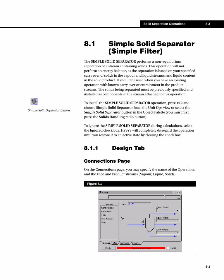
Solid Separation Operations 8-3
8.1 Simple Solid Separator (Simple Filter)
The SIMPLE SOLID SEPARATOR performs a non-equilibrium separation of a stream containing solids. This operation will not perform an energy balance, as the separation is based on your specified carry over of solids in the vapour and liquid streams, and liquid content in the solid product. It should be used when you have an existing operation with known carry over or entrainment in the product streams. The solids being separated must be previously specified and installed as components in the stream attached to this operation.
To install the SIMPLE SOLID SEPARATOR operation, press F12 and choose Simple Solid Separator from the Unit Ops view or select the Simple Solid Separator button in the Object Palette (you must first press the Solids Handling radio button).
To ignore the SIMPLE SOLID SEPARATOR during calculations, select the Ignored check box. HYSYS will completely disregard the operation until you restore it to an active state by clearing the check box.
8.1.1 Design Tab
Connections Page
On the Connections page, you may specify the name of the Operation, and the Feed and Product streams (Vapour, Liquid, Solids).
Figure 8.1
Simple Solid Separator Button
8-3
8-4 Simple Solid Separator (Simple Filter)
8-4
Parameters Page
You may specify the Pressure drop on the Parameters page.
Splits Page
On the Splits page, you must choose the split method by defining a Type of Fraction:
In the Flowsheet, the streams will not be reported as single phase, due to the solid content in the vapour and liquid streams, and the liquid content in the solid product stream.
User Variables Page
The User Variables page allows you to create and implement variables in the HYSYS simulation case. For more information on implementing the User Variables option, see User Variables chapter in the Customization Guide.
Notes Page
The Notes page provides a text editor where you can record any comments or information regarding the unit operation or pertaining to your simulation, in general.
8.1.2 Rating TabThis unit operation does not currently have rating features.
Object Definition
Split Fractions
Specify the fractional distribution of solids from the feed into the vapour and liquid product streams. The solids fraction in the bottoms will be calculated by HYSYS. You must also specify the fraction of liquid in the bottoms (solid product).
Stream Fractions
Enter the mole, mass or liquid volume fraction specification for each of the following:
• total vapour product solids fraction on the specified basis
• total liquid product solids fraction on the specified basis
• liquid phase fraction in the bottom product

Solid Separation Operations 8-5
8.1.3 Worksheet TabThe Worksheet tab contains a summary of the information contained in the Stream property view for all the streams attached to the unit operation. The Conditions, Properties, and Composition pages contain selected information from the corresponding pages of the Worksheet tab for the Stream property view.
8.1.4 Dynamics TabThis unit operation is currently not available for dynamic simulation.
8.2 CycloneThe CYCLONE is used to separate solids from a gas stream and is recommended only for particle sizes greater than 5 microns. The CYCLONE consists of a vertical cylinder with a conical bottom, a rectangular inlet near the top, and an outlet for solids at the bottom of the cone. It is the centrifugal force developed in the vortex which moves the particles toward the wall. Particles which reach the wall, slide down the cone, and so become separated from the gas stream. The solids being separated must be previously specified and installed as components in the stream attached to this operation.
To install the CYCLONE operation, press F12 and choose Cyclone from the Unit Ops view or select the Cyclone button in the Object Palette (you must first press the Solids Handling radio button).
To ignore the CYCLONE during calculations, select the Ignored check box. HYSYS will completely disregard the operation until you restore it to an active state by clearing the check box.
Cyclone Button
8-5
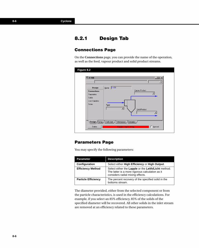
8-6 Cyclone
8-6
8.2.1 Design Tab
Connections Page
On the Connections page, you can provide the name of the operation, as well as the feed, vapour product and solid product streams.
Parameters Page
You may specify the following parameters:
The diameter provided, either from the selected component or from the particle characteristics, is used in the efficiency calculations. For example, if you select an 85% efficiency, 85% of the solids of the specified diameter will be recovered. All other solids in the inlet stream are removed at an efficiency related to these parameters.
Figure 8.2
Parameter Description
Configuration Select either High Efficiency or High Output.
Efficiency Method Select either the Lapple or the Leith/Licht method. The latter is a more rigorous calculation as it considers radial mixing effects.
Particle Efficiency The percent recovery of the specified solid in the bottoms stream.
Solid Separation Operations 8-7
Solids Page
On the this page the following solids information can be specified:
User Variables Page
The User Variables page allows you to create and implement variables in the HYSYS simulation case. For more information on implementing the User Variables option, see the User Variables chapter in the Customization Guide.
Notes Page
The Notes page provides a text editor where you can record any comments or information regarding the unit operation or pertaining to your simulation, in general.
8.2.2 Ratings Tab
Sizing Page
Specify the following parameters:
Parameter Description
Solid Name You must provide either the name of a solid already installed in the case (accessed through the Edit Bar), or provide a particle diameter and density.
Particle Diameter and Particle Density
If you do not choose a Solid component, provide the particle diameter and density.
Parameter Description
Configuration Select High Output, High Efficiency, or User Defined. This is also defined on the Parameters page.
Inlet Width Ratio The ratio of the inlet width to the body diameter (must be between 0 and 1).
The value must be less than the Total Height Ratio
Inlet Height Ratio The ratio of the inlet height to the body diameter.
Cyclone Height Ratio
The ratio of the cyclone height to the body diameter. The cyclone is the conical section at the bottom of the entire operation.
Gas Outlet Length Ratio
The ratio of the gas outlet length to the body diameter.
8-7
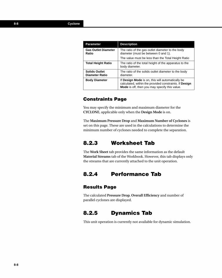
8-8 Cyclone
8-8
Constraints Page
You may specify the minimum and maximum diameter for the CYCLONE, applicable only when the Design Mode is on.
The Maximum Pressure Drop and Maximum Number of Cyclones is set on this page. These are used in the calculations to determine the minimum number of cyclones needed to complete the separation.
8.2.3 Worksheet TabThe Work Sheet tab provides the same information as the default Material Streams tab of the Workbook. However, this tab displays only the streams that are currently attached to the unit operation.
8.2.4 Performance Tab
Results Page
The calculated Pressure Drop, Overall Efficiency and number of parallel cyclones are displayed.
8.2.5 Dynamics TabThis unit operation is currently not available for dynamic simulation.
Gas Outlet Diameter Ratio
The ratio of the gas outlet diameter to the body diameter (must be between 0 and 1).
The value must be less than the Total Height Ratio
Total Height Ratio The ratio of the total height of the apparatus to the body diameter.
Solids Outlet Diameter Ratio
The ratio of the solids outlet diameter to the body diameter.
Body Diameter If Design Mode is on, this will automatically be calculated, within the provided constraints. If Design Mode is off, then you may specify this value.
Parameter Description
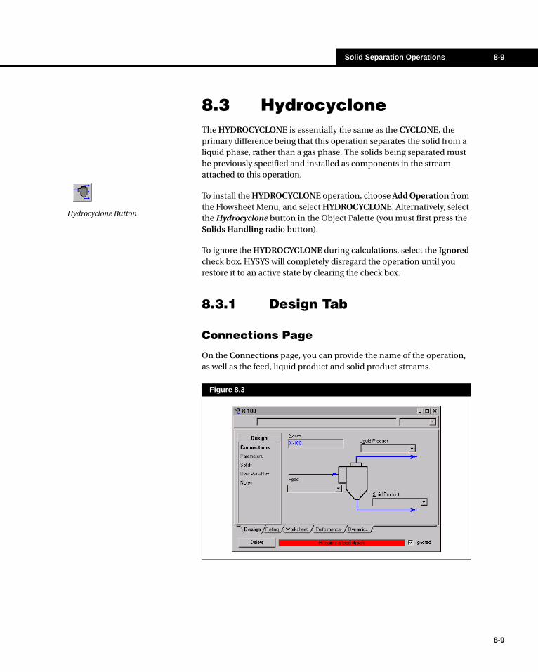
Solid Separation Operations 8-9
8.3 HydrocycloneThe HYDROCYCLONE is essentially the same as the CYCLONE, the primary difference being that this operation separates the solid from a liquid phase, rather than a gas phase. The solids being separated must be previously specified and installed as components in the stream attached to this operation.
To install the HYDROCYCLONE operation, choose Add Operation from the Flowsheet Menu, and select HYDROCYCLONE. Alternatively, select the Hydrocyclone button in the Object Palette (you must first press the Solids Handling radio button).
To ignore the HYDROCYCLONE during calculations, select the Ignored check box. HYSYS will completely disregard the operation until you restore it to an active state by clearing the check box.
8.3.1 Design Tab
Connections Page
On the Connections page, you can provide the name of the operation, as well as the feed, liquid product and solid product streams.
Figure 8.3
Hydrocyclone Button
8-9

8-10 Hydrocyclone
8-10
Parameters Page
You may specify the following parameters:
The diameter provided, either from the selected component or from the particle characteristics, is used in the efficiency calculations. For example, if you select an 85% efficiency, 85% of the solids of the specified diameter will be recovered. All other solids in the inlet stream are removed at an efficiency related to these parameters.
Solids Page
The following solids information may be specified:
User Variables Page
The User Variables page allows you to create and implement variables in the HYSYS simulation case. For more information on implementing the User Variables option, see the User Variables chapter in the Customization Guide.
Notes Page
The Notes page provides a text editor where you can record any comments or information regarding the unit operation, or pertaining to your simulation in general.
Parameter Description
Configuration Select either Mode 1, Mode 2, or User Defined.
Particle Efficiency The percent recovery of the specified solid in the bottoms stream.
Parameter Description
Solid Name You must provide either the name of a solid already installed in the case (accessed from the drop down menu in the Edit Bar), or provide a particle diameter and density.
Particle Diameter and Particle Density
If you do not specify a Solid Name, provide the particle diameter and density.
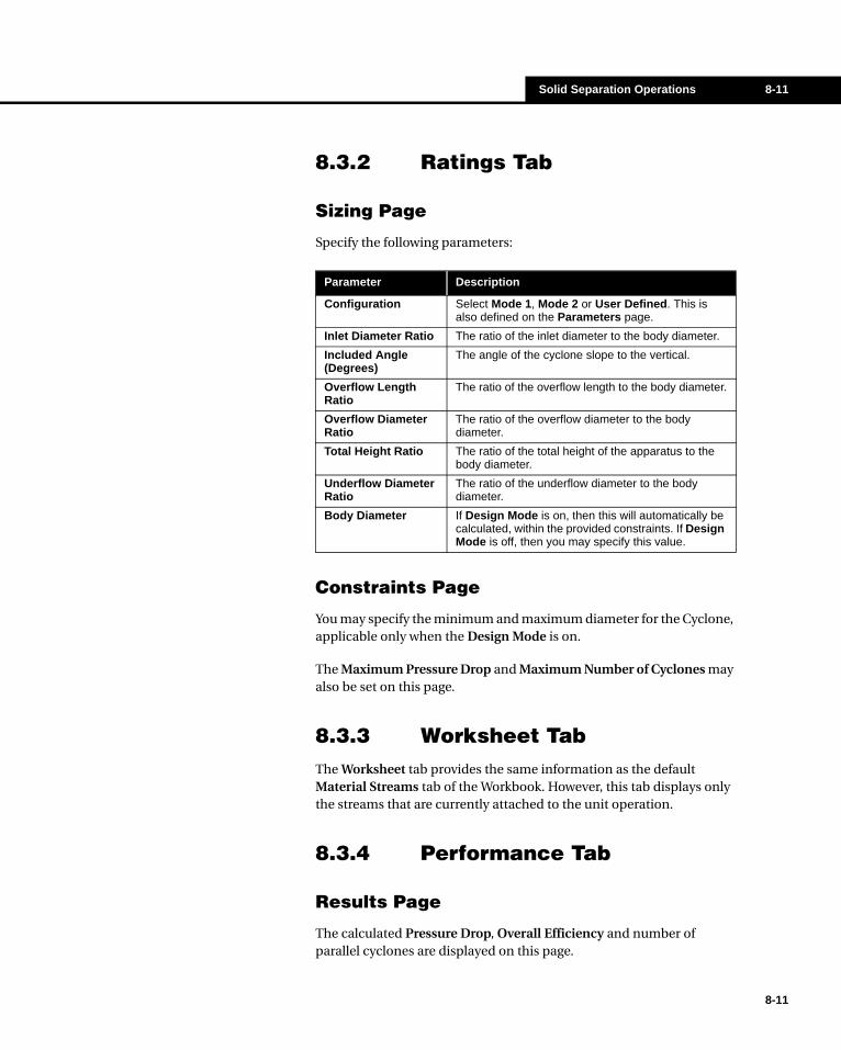
Solid Separation Operations 8-11
8.3.2 Ratings Tab
Sizing Page
Specify the following parameters:
Constraints Page
You may specify the minimum and maximum diameter for the Cyclone, applicable only when the Design Mode is on.
The Maximum Pressure Drop and Maximum Number of Cyclones may also be set on this page.
8.3.3 Worksheet TabThe Worksheet tab provides the same information as the default Material Streams tab of the Workbook. However, this tab displays only the streams that are currently attached to the unit operation.
8.3.4 Performance Tab
Results Page
The calculated Pressure Drop, Overall Efficiency and number of parallel cyclones are displayed on this page.
Parameter Description
Configuration Select Mode 1, Mode 2 or User Defined. This is also defined on the Parameters page.
Inlet Diameter Ratio The ratio of the inlet diameter to the body diameter.
Included Angle (Degrees)
The angle of the cyclone slope to the vertical.
Overflow Length Ratio
The ratio of the overflow length to the body diameter.
Overflow Diameter Ratio
The ratio of the overflow diameter to the body diameter.
Total Height Ratio The ratio of the total height of the apparatus to the body diameter.
Underflow Diameter Ratio
The ratio of the underflow diameter to the body diameter.
Body Diameter If Design Mode is on, then this will automatically be calculated, within the provided constraints. If Design Mode is off, then you may specify this value.
8-11

8-12 Rotary Vacuum Filter
8-12
8.3.5 Dynamics TabThis unit operation is currently not available for dynamic simulation.
8.4 Rotary Vacuum FilterThe ROTARY VACUUM FILTER assumes that there is 100% removal of the solid from the solvent stream. This operation will determine the retention of solvent in the particle cake, based on the particle diameter and sphericity of your defined solid(s). The diameter and sphericity determines the capillary space in the cake and thus the solvent retention. The solids being separated must be previously specified and installed as components in the stream attached to this operation.
To install the ROTARY VACUUM FILTER operation, press F12 and choose Rotary Vacuum Filter from the Unit Ops view or select the Rotary Vacuum Filter button in the Object Palette (you must first press the Solids Handling radio button).
To ignore the operation during calculations, select the Ignored check box. HYSYS will completely disregard the operation until you restore it to an active state by clearing the check box.
8.4.1 Design Tab
Connections Page
On the Connections page, define the Operation Name, as well as the Feed, Liquid Product and Solids Product streams.
Rotary Vacuum Filter Button
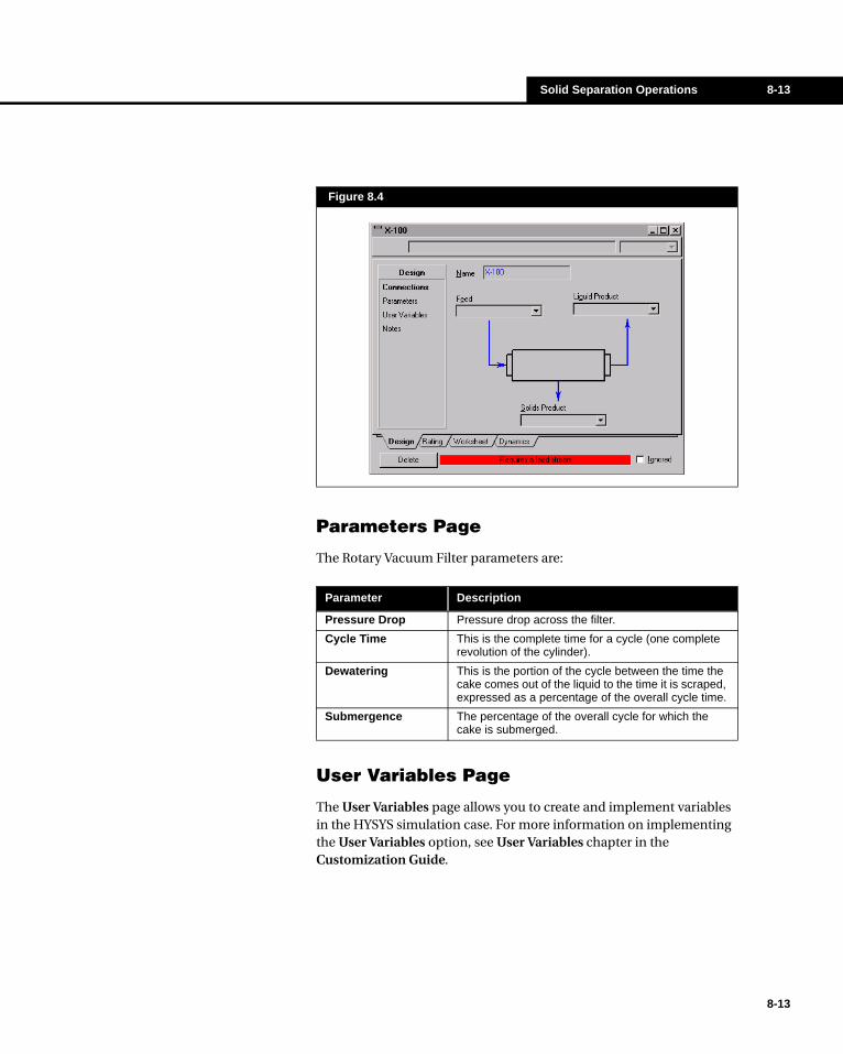
Solid Separation Operations 8-13
Parameters Page
The Rotary Vacuum Filter parameters are:
User Variables Page
The User Variables page allows you to create and implement variables in the HYSYS simulation case. For more information on implementing the User Variables option, see User Variables chapter in the Customization Guide.
Figure 8.4
Parameter Description
Pressure Drop Pressure drop across the filter.
Cycle Time This is the complete time for a cycle (one complete revolution of the cylinder).
Dewatering This is the portion of the cycle between the time the cake comes out of the liquid to the time it is scraped, expressed as a percentage of the overall cycle time.
Submergence The percentage of the overall cycle for which the cake is submerged.
8-13
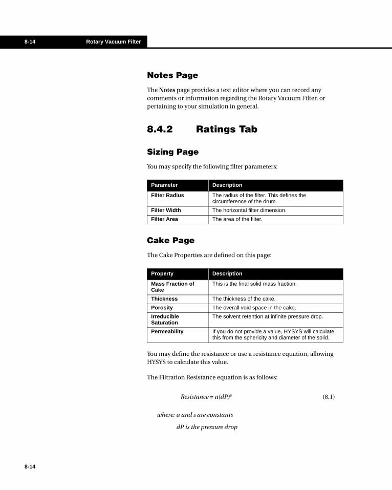
8-14 Rotary Vacuum Filter
8-14
Notes Page
The Notes page provides a text editor where you can record any comments or information regarding the Rotary Vacuum Filter, or pertaining to your simulation in general.
8.4.2 Ratings Tab
Sizing Page
You may specify the following filter parameters:
Cake Page
The Cake Properties are defined on this page:
You may define the resistance or use a resistance equation, allowing HYSYS to calculate this value.
The Filtration Resistance equation is as follows:
where: a and s are constants
dP is the pressure drop
Parameter Description
Filter Radius The radius of the filter. This defines the circumference of the drum.
Filter Width The horizontal filter dimension.
Filter Area The area of the filter.
Property Description
Mass Fraction of Cake
This is the final solid mass fraction.
Thickness The thickness of the cake.
Porosity The overall void space in the cake.
Irreducible Saturation
The solvent retention at infinite pressure drop.
Permeability If you do not provide a value, HYSYS will calculate this from the sphericity and diameter of the solid.
Resistance = a(dP)s (8.1)

Solid Separation Operations 8-15
8.4.3 Worksheet TabThe Worksheet tab provides the same information as the default Material Streams tab of the Workbook. However, this tab displays only the streams that are currently attached to the unit operation.
8.4.4 Dynamics TabThis unit operation is currently not available for dynamic simulation.
8.5 Baghouse FilterThe BAGHOUSE FILTER model is based on empirical equations. It contains an internal curve relating separation efficiency to particle size. Based on your particle diameter, the reported separation efficiency for your solids will be determined from this curve. The solids being separated must be previously specified and installed as components in the stream attached to this operation.
To install the BAGHOUSE FILTER operation, press F12 and choose Baghouse Filter from the Unit Ops view or select the Baghouse Filter button in the Object Palette (you must first press the Solids Handling radio button).
To ignore the BAGHOUSE FILTER during calculations, select the Ignored check box. HYSYS will completely disregard the operation until you restore it to an active state by clearing the check box.
8.5.1 Design Tab
Connections Page
On the Connections page, supply the name of the operation, as well as the feed, vapour product and solid product streams.
Baghouse Filter Button
8-15

8-16 Baghouse Filter
8-16
Parameters Page
On the Parameters page, you must supply the following information:
User Variables Page
The User Variables page allows you to create and implement variables in the HYSYS simulation case. For more information on implementing the User Variables option, see the User Variables chapter in the on-line Customization Guide.
Notes Page
The Notes page provides a text editor where you can record any comments or information regarding the unit operation or pertaining to your simulation, in general.
Figure 8.5
Parameter Description
Configuration When you make a change to any of the parameters, the configuration will change to User Defined. Select Default to revert to the HYSYS defaults.
Clean Bag Pressure Drop
The pressure drop across a clean bag.
Dirty Bag Pressure Drop
The pressure drop across a dirty bag. This value must be greater than the Clean Bag Pressure Drop.
Solid Separation Operations 8-17
8.5.2 Rating Tab
Sizing Page
The following parameters may be specified:
8.5.3 Worksheet TabThe Worksheet tab provides the same information as the default Material Streams tab of the Workbook. However, this tab displays only the streams that are currently attached to the unit operation.
8.5.4 Performance Tab
Results page
The following Filtration results are displayed on this page:
• Filtration Time• Number of Cells• Area/Cell• Total Cell Area• Particle Diameter
8.5.5 Dynamics TabThis unit operation is currently not available for dynamic simulation.
Parameter Description
Maximum Gas Velocity
Maximum velocity of gas in the Baghouse filter.
Bag Filter Area Filter Area for each bag.
Bag Diameter Bag Diameter.
Bags per Cell Number of bags per filter cell.
Bag Spacing Spacing between the bags.
8-17

8-18 Baghouse Filter
8-18

Reactors 9-1
9 Reactors
9.1 The Reactor Operation................................................................................. 3
9.2 CSTR / General Reactor Design Tab........................................................... 4
9.2.1 Connections Page.................................................................................... 59.2.2 Parameters Page ..................................................................................... 6
9.3 CSTR / General Reactor Reactions Tab ..................................................... 8
9.3.1 Conversion Reactor Reactions Tab.......................................................... 89.3.2 CSTR Reactions Tab.............................................................................. 139.3.3 Equilibrium Reactor - Reaction Tab........................................................ 179.3.4 Gibbs Reactor Reactions Tab ................................................................ 22
9.4 CSTR / General Reactor Rating Tab ......................................................... 25
9.5 CSTR / General Reactor Work Sheet Tab................................................. 29
9.6 CSTR / General Reactor Dynamics Tab.................................................... 29
9.7 Plug Flow Reactor (PFR) Property View .................................................. 29
9.7.1 PFR Design Tab..................................................................................... 309.7.2 Reactions Tab ........................................................................................ 379.7.3 Ratings Tab ............................................................................................ 459.7.4 Work Sheet Tab...................................................................................... 469.7.5 Performance Tab.................................................................................... 479.7.6 Dynamics Tab ........................................................................................ 499.7.7 PFR Example Problem........................................................................... 49
9-1

9-2
9-2

Reactors 9-3
9.1 The Reactor OperationWith the exception of the PLUG FLOW REACTOR (PFR), all of the reactor operations share the same basic property view. The primary differences are the functions of the reaction type (conversion, kinetic, equilibrium, heterogeneous catalytic or simple rate) associated with each reactor. As opposed to a SEPARATOR or GENERAL REACTOR with an attached reaction set, specific reactor operations may only support one particular reaction type. For instance, a CONVERSION REACTOR will only function properly with conversion reactions attached. If you try to attach an equilibrium or a kinetic reaction to a CONVERSION REACTOR, an error message will appear. The GIBBS REACTOR is unique in that it can function with or without a reaction set.
You have great deal flexibility in defining and grouping reactions. You may:
• Define the reactions inside the Basis Manager, group them into a set and then attach the set to your reactor.
• Create reactions in the Reaction Package in the Main Flowsheet, group them into a set and attach the set to the reactor.
• Create reactions and reaction sets in the Basis Environment and make changes in the Main Environment's Reaction Package.
Regardless of the approach, the reactions you define will be visible to the entire Flowsheet, i.e. a reaction set can be attached to more than one reactor.
However, there are some subtleties of which you must be aware. When you make a modification to a reaction via a reactor, the change is only seen locally, in that particular reactor. Modifications made to a reaction in the Basis Environment or in the Reaction Package are automatically reflected in every reactor using the reaction set, provided you have not made changes locally. Local changes are always retained. To override local changes and return the global parameters to a reaction, you must press the DELETE key when the cursor is in the cell which contains the local change.
The four reactors which share common property views include:
• CSTR (Continuous-Stirred Tank Reactor)• GIBBS REACTOR• EQUILIBRIUM REACTOR• CONVERSION REACTOR
Refer to Chapter 4 - Reactions of the Simulation Basis manual or Section 7.4.1 - Reaction Package of the User’s Guide for details on installing reactions and Reaction Sets.
9-3

9-4 CSTR / General Reactor Design Tab
9-4
The last three reactors are referred to as General Reactors. In order to avoid redundancy, these operations will be discussed co-currently. In areas of the property view where there are differences, such as the Reactions tab, the differences will be clearly noted.
The PLUG FLOW REACTOR, or PFR, has quite a different property views from the other reactors. As a result it will be discussed on its own in Section 9.7 - Plug Flow Reactor (PFR) Property View.
A Reactor operation can be installed by pressing F12 and selecting the operation from the UnitOps view or by selecting the appropriate button from the Object Palette. In order to implement a GIBBS, CONVERSION or EQUILIBRIUM reactor, you must first press the General Reactors button to access the distinct button for each Reactor type in the Object Palette.
9.2 CSTR / General Reactor Design Tab
The CSTR and GENERAL Reactors property view consists of five tabs the first of which is the Design tab. It contains four pages:
To remove local changes, move to the appropriate cell and press the DELETE key.
General Reactors Button
Conversion Reactors Button
Equilibrium Reactors Button
Gibbs Reactor Button
CSTR (Continuous-Stirred Tank Reactor) Button
Page Description
Connections Connects the feed, product, and energy streams to the reactor.
Parameters Set heat transfer and pressure drop parameters for the reactor.
User Variables Allows for the creation and implementation of User Variables.
Notes Allows you to add relevant comments which are exclusively associated with this unit operation.

Reactors 9-5
9.2.1 Connections Page
The Connections page, is the same for both the CSTR and the three General Reactors. The page consists of 5 objects:
Figure 9.1
Object Input Required
NameContains the name of the reactor. You may edit the Name at any time by simply selecting the field (double click the cursor inside the field) and inputting a new name.
Inlets
Allows for the connection of a single feed or multiple feed streams to the reactor. You may either attach the feed stream(s) by selecting previously created streams from the drop down in the Edit Bar, or by selecting an empty cell in the Inlets matrix and entering a new stream name in the Edit Bar.
Vapour Outlet
Connects the Vapour product stream to the Reactor. As with the Inlets field, you may select an existing stream from the drop down or create a new product stream by selecting the field and typing the new stream name in the Edit Bar
Liquid Outlet
Connects the Liquid product stream to the Reactor. As with the Feeds field, you may select an existing stream from the drop down or create a new product stream by selecting the field and typing the new stream name in the Edit Bar
Energy (Optional)
Allows for the connection or creation of an energy stream if one is required for this operation.
At least one product stream is required.
9-5

9-6 CSTR / General Reactor Design Tab
9-6
9.2.2 Parameters Page
The Parameters page allows you to specify the Pressure Drop, Vessel Volume, Duty and Solving Behaviour.
Figure 9.2
Note that Pfeed is assumed to be the lowest pressure of all the feed streams.
Object Description
Delta P
This field contains the pressure drop across the vessel. The pressure drop is defined as:
(9.1)
where: P = Vessel pressure
Pv = Pressure of vapour product stream
Pl = Pressure of liquid product stream
Pfeed = Pressure of feed stream
∆P = Pressure drop in vessel (Delta P)
The default pressure drop across the vessel is zero.
The vessel pressure is used in the reaction calculations.
∆P P Pv– P Pl–= =

Reactors 9-7
Duty
If you have attached an energy stream, you can specify that it is to be used for heating or for cooling by selecting the appropriate radio button. You also have a choice of specifying the applied duty, or having HYSYS calculate the duty. For the latter case, you must specify an outlet temperature for a reactor product stream.
The Steady-State Reactor energy balance is defined below
(9.2)
where: Duty = the heating (+ve) or cooling (-ve) by the optional energy stream
Hvapour = Heat flow of the vapour product stream
Hliquid = Heat flow of the liquid product stream
Hfeed = Heat flow of the feed stream(s)
Heating /Cooling
If you change from Heating to Cooling (or vice versa), the magnitude of the energy stream does not change. However, the sign will change in the energy balance. For Heating, the duty is added. For Cooling, the duty is subtracted.
Volume
User specified, this is the total volume of the vessel. While not necessarily required for solving CONVERSION, GIBBS, or EQUILIBRIUM reactors in Steady State mode, this value must be entered for CSTR.
The Vessel Volume, together with the Liquid Level set point, define the amount of holdup in the Vessel. The amount of liquid volume, or holdup, in the vessel at any time is given by the following expression:
(9.3)
where: PV(%Full) is the liquid level in the vessel.
Liquid Level Displays the liquid level of the reactor expressed as a percentage of the Full Vessel Volume.
Liquid Volume
Not set by the user, this value is calculated from the product of the Volume (Vessel Volume) and Liquid Level fraction. It is only active when the Volume field contains a valid entry.
Act as a Separator When Cannot Solve
Only available for CONVERSION and EQUILIBRIUM reactors, this option allows you to operate the reactor as a simple 2 phase separator whenever the reactor does not solve.
Single Phase Allows for the specification of a single phase reaction. Otherwise HYSYS will consider it a vapour-liquid reaction.
Type
Only available for Gibbs reactors, this gives you a choice regarding the type of reactor you require:
• Separator - applies a two phase Gibbs minimization to the reactants.
• Three Phase - applies a three phase Gibbs minimization to the reactants.
Object Description
Note that the enthalpy basis used by HYSYS is equal to the ideal gas enthalpy of formation at 25 °C and 1 atm. As a result, the heat of reaction calculation is amalgamated into any product/reactant enthalpy difference.
Duty Hvapour Hliquid Hfeed–+=
The Vessel Volume is necessary when modelling reactors in Steady State, as it determines the residence time.
Holdup Vessel VolumePV %Full( )
100-----------------------------×=
9-7

9-8 CSTR / General Reactor Reactions Tab
9-8
To ignore the unit operation entirely during calculations, select the Ignored check box. HYSYS will disregard the operation entirely until you restore it to an active state.
9.3 CSTR / General Reactor Reactions Tab
9.3.1 Conversion Reactor Reactions Tab
The CONVERSION REACTOR is a vessel in which Conversion reactions are performed. You may only attach Reaction Sets that contain Conversion Reactions. Each reaction in the set will proceed until the specified conversion is attained or until a limiting reactant is depleted.
The Reactions tab, consists of two pages: Details and Results.
Details Page
Figure 9.3
Conversion Reactor
Refer to Section 4.4.2 - Conversion Reaction of the Simulation Basis guide for details on creating Conversion Reaction Sets and Conversion Reactions.

Reactors 9-9
On this page you can attach the Reaction Set to the operation and specify the conversion for each reaction in the set. The Reaction Set can contain only conversion reactions. The page is split into 4 objects:
Stoichiometry Radio Button
The Stoichiometry group allows you to examine the components involved in the selected reaction, their molecular weights as well as their stoichiometric coefficients. The Balance Error and the Reaction Heat (Heat of Reaction) are also shown for the current reaction.
Object Description
Reaction Set Allows you to select the appropriate Conversion Reaction Set.
Reaction You must select the appropriate Conversion reaction from the selected Reaction Set.
View ReactionOpens the Reaction property view for the reaction currently selected in the Reaction drop down. This allows you to edit the reaction.
[Radio buttons]
These three radio buttons toggles between the Stoichiometry group box, the Basis group box or the Conversion group box (each described in the following subsections).
Figure 9.4
9-9

9-10 CSTR / General Reactor Reactions Tab
9-10
Basis Radio Button
In the Basis group, you can view the Base Component, the Conversion and the Reaction Phase for each reaction in the Reaction Set. Here, you may also change the local specified conversion.
Conversion Radio Button
In the Fractional Conversion Equation group allows implementation of a conversion model based on the Conversion(%) equation listed. The parameters for the attached conversion reaction(s) can be cloned as local variables belonging to the Conversion Reactor. Therefore a user can either use the parameters specified in the reaction(s) from the attached reaction set by selecting the Use Default cross box or specify locally the values within the Fractional Conversion Equation group.
Figure 9.5
Figure 9.6
Note that in the Fractional Conversion Equation group box, spaces showing red or blue colour indicate that the variable may be cloned.

Reactors 9-11
View Reaction Button
Pressing this button opens the Conversion Reaction property view of the reaction currently selected in the Reaction drop down box. Note that any changes made to the Conversion Reaction property view will be made globally to the selected Reaction and any Reaction Sets which contain the Reaction. For example, if any change is made to the reaction shown in Figure 9.7, the change will be carried over to every other instance in which this Reaction is used. It is therefore recommended that changes which are Reactor specific (i.e. changes which are only meant to affect one Reactor) are made within the Reactions tab.
Results Page
The Results page displays the results of a converged reactor. The page is made up of the Reactor Results Summary group box which contains two radio buttons: Reaction Extents and Reaction Balance. The type of results displayed depends on which radio button is active.
Figure 9.7
You can change the specified conversion for a reaction directly on this page.
9-11
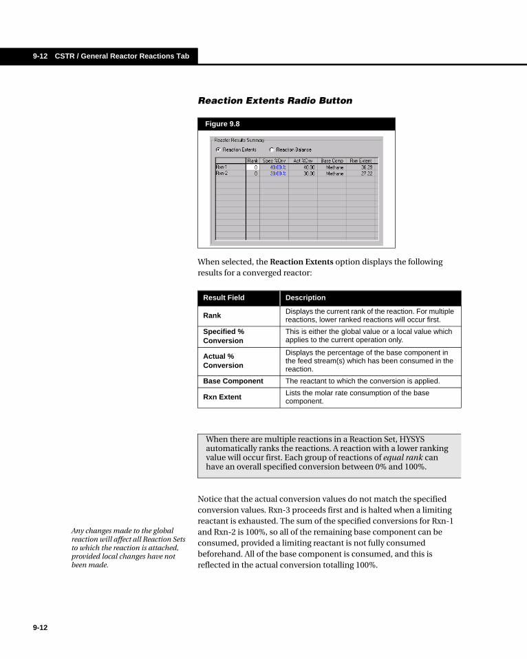
9-12 CSTR / General Reactor Reactions Tab
9-12
Reaction Extents Radio Button
When selected, the Reaction Extents option displays the following results for a converged reactor:
Notice that the actual conversion values do not match the specified conversion values. Rxn-3 proceeds first and is halted when a limiting reactant is exhausted. The sum of the specified conversions for Rxn-1 and Rxn-2 is 100%, so all of the remaining base component can be consumed, provided a limiting reactant is not fully consumed beforehand. All of the base component is consumed, and this is reflected in the actual conversion totalling 100%.
Figure 9.8
Result Field Description
Rank Displays the current rank of the reaction. For multiple reactions, lower ranked reactions will occur first.
Specified % Conversion
This is either the global value or a local value which applies to the current operation only.
Actual % Conversion
Displays the percentage of the base component in the feed stream(s) which has been consumed in the reaction.
Base Component The reactant to which the conversion is applied.
Rxn Extent Lists the molar rate consumption of the base component.
When there are multiple reactions in a Reaction Set, HYSYS automatically ranks the reactions. A reaction with a lower ranking value will occur first. Each group of reactions of equal rank can have an overall specified conversion between 0% and 100%.
Any changes made to the global reaction will affect all Reaction Sets to which the reaction is attached, provided local changes have not been made.

Reactors 9-13
Reaction Balance Radio Button
When selected, the Reaction Balance option provides an overall component summary for the CONVERSION REACTOR. All components which appear in the Fluid Package are shown here.
Values appear after all reactions have been completed. The Total Inflow rate, the Total Reacted rate and the Total Outflow rate for each component are provided on a molar basis. Negative values indicate the consumption of a reactant, while positive values indicate the appearance of a product.
9.3.2 CSTR Reactions TabThe CSTR is a vessel in which Kinetic, Heterogeneous Catalytic and Simple Rate reactions can be performed. The conversion in the reactor depends on the rate expression of the reactions associated with the reaction type. The inlet stream is assumed to be perfectly (and instantaneously) mixed with the material already in the reactor, so that the outlet stream composition is identical to that of the reactor contents. Given the reactor volume, a consistent rate expression for each reaction and the reaction stoichiometry, the CSTR computes the conversion of each component entering the reactor.
On the Reactions tab, you can select a Reaction Set for the operation. You may also view the results of the solved reactor including the actual conversion of the Base Component. The actual conversion is calculated as the percentage of the base component that was consumed in the reaction.
Figure 9.9
For more information on Kinetic, Heterogeneous Catalytic and Simple Rate reactions see Chapter 4 - Reactions of the Simulation Basis guide.
CSTR Button
(9.4)XNAin
NAout–
NAin
---------------------------- 100%×=
9-13
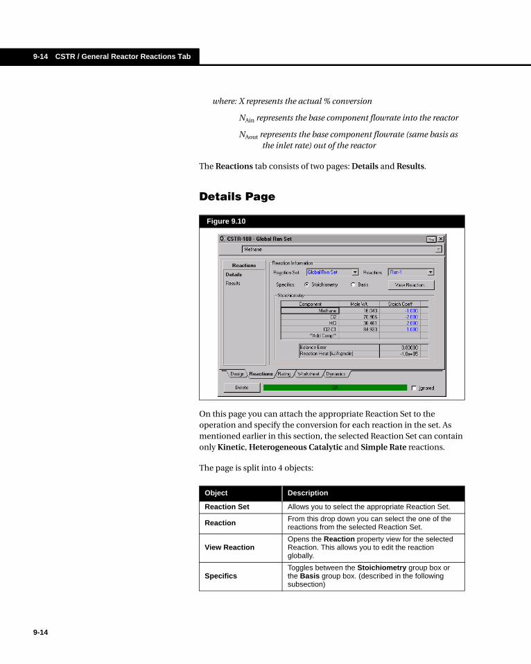
9-14 CSTR / General Reactor Reactions Tab
9-14
where: X represents the actual % conversion
NAin represents the base component flowrate into the reactor
NAout represents the base component flowrate (same basis as the inlet rate) out of the reactor
The Reactions tab consists of two pages: Details and Results.
Details Page
On this page you can attach the appropriate Reaction Set to the operation and specify the conversion for each reaction in the set. As mentioned earlier in this section, the selected Reaction Set can contain only Kinetic, Heterogeneous Catalytic and Simple Rate reactions.
The page is split into 4 objects:
Figure 9.10
Object Description
Reaction Set Allows you to select the appropriate Reaction Set.
Reaction From this drop down you can select the one of the reactions from the selected Reaction Set.
View ReactionOpens the Reaction property view for the selected Reaction. This allows you to edit the reaction globally.
SpecificsToggles between the Stoichiometry group box or the Basis group box. (described in the following subsection)
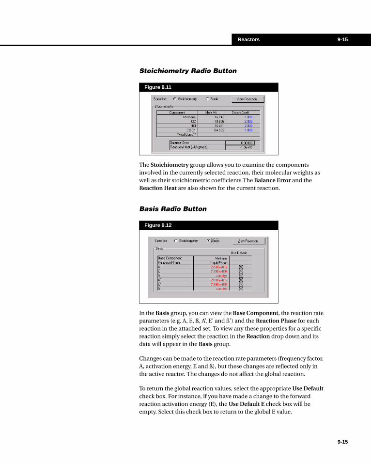
Reactors 9-15
Stoichiometry Radio Button
The Stoichiometry group allows you to examine the components involved in the currently selected reaction, their molecular weights as well as their stoichiometric coefficients.The Balance Error and the Reaction Heat are also shown for the current reaction.
Basis Radio Button
In the Basis group, you can view the Base Component, the reaction rate parameters (e.g. A, E, ß, A’, E’ and ß’) and the Reaction Phase for each reaction in the attached set. To view any these properties for a specific reaction simply select the reaction in the Reaction drop down and its data will appear in the Basis group.
Changes can be made to the reaction rate parameters (frequency factor, A, activation energy, E and ß), but these changes are reflected only in the active reactor. The changes do not affect the global reaction.
To return the global reaction values, select the appropriate Use Default check box. For instance, if you have made a change to the forward reaction activation energy (E), the Use Default E check box will be empty. Select this check box to return to the global E value.
Figure 9.11
Figure 9.12
9-15

9-16 CSTR / General Reactor Reactions Tab
9-16
Results Page
The Results page displays the results of a converged reactor. The page is made up of the Reaction Results Summary group box which contains two radio buttons: Reaction Extents and Reaction Balance.
Reaction Extents Radio Button
When selected, the Reaction Extents option will display the following results for a converged reactor:
Figure 9.13
Result Field Description
Actual % Conversion
Displays the percentage of the base component in the feed stream(s) which has been consumed in the reaction.
Base Component The reactant to which the conversion is applied.
Rxn Extent Lists the molar rate of consumption of the base component.

Reactors 9-17
Reaction Balance Radio Button
When selected the Reaction Balance option provides an overall component summary for the CSTR. All components which appear in the Fluid Package are shown here.
Values appear after all reactions have been completed. The Total Inflow rate, the Total Reacted rate and the Total Outflow rate for each component are provided on a molar basis. Negative values indicate the consumption of a reactant, while positive values indicate the appearance of a product.
9.3.3 Equilibrium Reactor - Reaction Tab
The Equilibrium reactor is a vessel which models equilibrium reactions. The outlet streams of the reactor are in a state of chemical and physical equilibrium. The Reaction Set which you attach to the EQUILIBRIUM REACTOR can contain an unlimited number of equilibrium reactions, which will be simultaneously or sequentially solved. Neither the components nor the mixing process need be ideal, since HYSYS can compute the chemical activity of each component in the mixture based on mixture and pure component fugacities.
You can also examine the actual conversion, the base component, the equilibrium constant and the reaction extent for each reaction in the selected Reaction Set. The conversion, the equilibrium constant and the extent are all calculated based on the equilibrium reaction information which you provided when the Reaction Set was created.
Figure 9.14
Equilibrium Reactor Button
Refer to Section 4.4.3 - Equilibrium Reaction of Simulation Basis guide for details on creating and installing Equilibrium Reactions.
Any changes made to the global reaction will affect all reaction sets to which the reaction is attached, provided local changes have not been made.
9-17
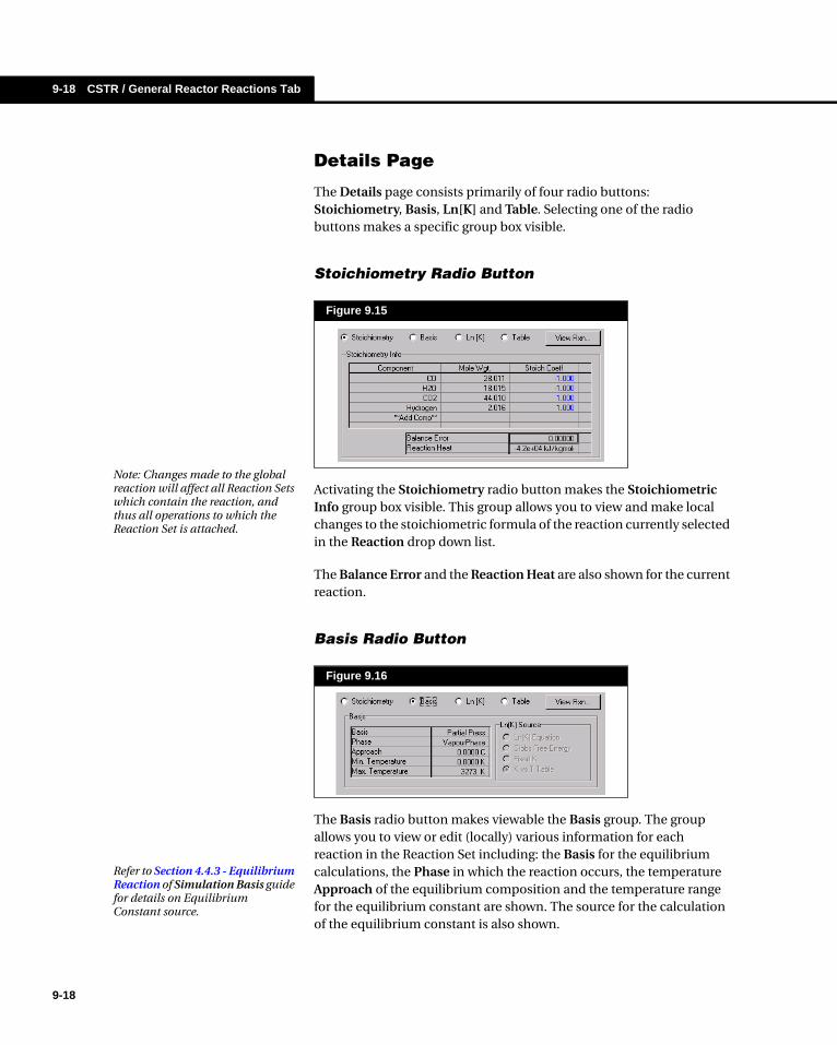
9-18 CSTR / General Reactor Reactions Tab
9-18
Details Page
The Details page consists primarily of four radio buttons: Stoichiometry, Basis, Ln[K] and Table. Selecting one of the radio buttons makes a specific group box visible.
Stoichiometry Radio Button
Activating the Stoichiometry radio button makes the Stoichiometric Info group box visible. This group allows you to view and make local changes to the stoichiometric formula of the reaction currently selected in the Reaction drop down list.
The Balance Error and the Reaction Heat are also shown for the current reaction.
Basis Radio Button
The Basis radio button makes viewable the Basis group. The group allows you to view or edit (locally) various information for each reaction in the Reaction Set including: the Basis for the equilibrium calculations, the Phase in which the reaction occurs, the temperature Approach of the equilibrium composition and the temperature range for the equilibrium constant are shown. The source for the calculation of the equilibrium constant is also shown.
Figure 9.15
Figure 9.16
Note: Changes made to the global reaction will affect all Reaction Sets which contain the reaction, and thus all operations to which the Reaction Set is attached.
Refer to Section 4.4.3 - Equilibrium Reaction of Simulation Basis guide for details on Equilibrium Constant source.
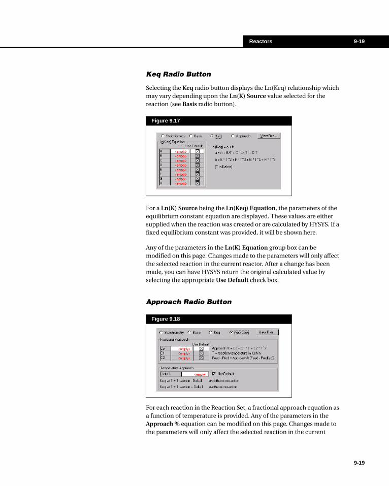
Reactors 9-19
Keq Radio Button
Selecting the Keq radio button displays the Ln(Keq) relationship which may vary depending upon the Ln(K) Source value selected for the reaction (see Basis radio button).
For a Ln(K) Source being the Ln(Keq) Equation, the parameters of the equilibrium constant equation are displayed. These values are either supplied when the reaction was created or are calculated by HYSYS. If a fixed equilibrium constant was provided, it will be shown here.
Any of the parameters in the Ln(K) Equation group box can be modified on this page. Changes made to the parameters will only affect the selected reaction in the current reactor. After a change has been made, you can have HYSYS return the original calculated value by selecting the appropriate Use Default check box.
Approach Radio Button
For each reaction in the Reaction Set, a fractional approach equation as a function of temperature is provided. Any of the parameters in the Approach % equation can be modified on this page. Changes made to the parameters will only affect the selected reaction in the current
Figure 9.17
Figure 9.18
9-19

9-20 CSTR / General Reactor Reactions Tab
9-20
reactor. After a change has been made, you can have HYSYS return the original calculated value by selecting the appropriate Use Default cross box.
You can edit a reaction by pressing the View Reaction button. The property view for the highlighted reaction appears.
Results Page
The Results page displays the results of a converged reactor. The page is made up of the Results Summary group box which contains two radio buttons: Reaction Extents and Reaction Balance.
Reaction Extents
When selected the Reaction Extents option will display the following results for a converged reactor:
Figure 9.19
For more detailed information on equilibrium reactions, see Chapter 4 - Reactions of Simulation Basis guide.
You can change the specified conversion for a reaction directly on this page.
Result Field Description
Actual % Conversion
Displays the percentage of base component in the feed stream(s) which has been consumed in the reaction.
The actual conversion is calculated as the percentage of the base component that was consumed in the reaction.
(9.5)
where: X represents the actual % conversion.
NAin represents the base component flowrate into the reactor.
NAout represents the base component flowrate (same basis as the inlet rate) out of the reactor.
XNAin
NAout–
NAin
---------------------------- 100%×=

Reactors 9-21
Reaction Balance
When selected, the Reaction Balance option provides an overall component summary for the EQUILIBRIUM REACTOR. All components which appear in the Fluid Package are shown here.
Values appear after all reactions have been completed. The Total Inflow rate, the Total Reacted rate and the Total Outflow rate for each component are provided on a molar basis. Negative values indicate the consumption of a reactant, while positive values indicate the appearance of a product.
Base Component
The reactant to which the conversion is applied.
Eqm Const.
The equilibrium constant is calculated at the reactor temperature by the following:
(9.6)
where: T represents the reactor temperature, in Kelvin
A, B, C, D are equation parameters
The four parameters in Equation (9.6) will be calculated by HYSYS if they are not supplied during the installation of the equilibrium reaction.
Rxn Extent Lists the molar rate consumption of the base component.
Result Field Description
The four parameters for each equilibrium equation are listed on the Rxn Ln(K) page.
Kln ABT--- C T DT+ln+ +=
Figure 9.20
9-21
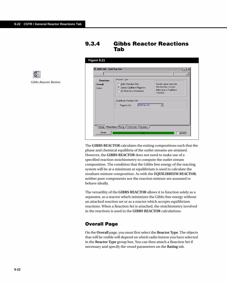
9-22 CSTR / General Reactor Reactions Tab
9-22
9.3.4 Gibbs Reactor Reactions Tab
The GIBBS REACTOR calculates the exiting compositions such that the phase and chemical equilibria of the outlet streams are attained. However, the GIBBS REACTOR does not need to make use of a specified reaction stoichiometry to compute the outlet stream composition. The condition that the Gibbs free energy of the reacting system will be at a minimum at equilibrium is used to calculate the resultant mixture composition. As with the EQUILIBRIUM REACTOR, neither pure components nor the reaction mixture are assumed to behave ideally.
The versatility of the GIBBS REACTOR allows it to function solely as a separator, as a reactor which minimizes the Gibbs free energy without an attached reaction set or as a reactor which accepts equilibrium reactions. When a Reaction Set is attached, the stoichiometry involved in the reactions is used in the GIBBS REACTOR calculations.
Overall Page
On the Overall page, you must first select the Reactor Type. The objects that will be visible will depend on which radio button you have selected in the Reactor Type group box. You can then attach a Reaction Set if necessary and specify the vessel parameters on the Rating tab.
Figure 9.21
Gibbs Reactor Button

Reactors 9-23
Reactor Type Group
In the Reactor Type group, choose a radio button to define the method which HYSYS will use to solve the GIBBS REACTOR:
Details Page
The Details page consists of one group box, the Gibbs Reaction Details group. The group box consists of two radio buttons: Flow Specs and Atom Matrix. The information that will be viewable on the page depends on which of the two radio buttons is active.
Radio Button Description
Gibbs Reactions Only
No reaction set is required as HYSYS solves the system by minimizing the Gibbs free energy while attaining phase and chemical equilibrium. Users may also customize the maximum iteration number and equilibrium error tolerance in the Solving Option group.
Specify Equilibrium Reactions
Will display the Equilibrium Reaction Sets group. When a reaction set is attached, the GIBBS REACTOR is solved using the stoichiometry of the reactions involved. The Gibbs minimization function uses the extents of the attached reactions while setting any unknowns to zero.
NO Reactions (=Separator)
The GIBBS REACTOR is solved as a separator operation, concerned only with phase equilibrium in the outlet streams.
9-23

9-24 CSTR / General Reactor Reactions Tab
9-24
Flow Specs Option
Selecting the Flow Specs radio button opens a view similar to the one seen in Figure 9.22. You can view the component feed and product flowrates on a molar basis. You can also designate any of the components as inert or specify a rate of production for a component.
Inert species are excluded from the Gibbs free energy minimization calculations. When the Inerts check box is activated for a component, values of 1 and 0 appear respectively in the associated Frac Spec and Fixed Spec cells, which indicates that the component feed flowrate will equal the product flowrate.
You may want to specify the rate of production of any component in your reactor as a constraint on the equilibrium composition. The component product flowrate will be calculated as follows, based on your input of a Frac Spec value and a Fixed Spec value:
The GIBBS reactor will attempt to meet that flowrate in calculating the outlet stream’s composition. If the constraint cannot be met, a message will be displayed alerting you to that effect.
Figure 9.22
Total Prod = FracSpec x Total Feed + FixedSpec (9.7)

Reactors 9-25
Atom Matrix Option
When the Atom Matrix radio button is active, you can specify the atomic composition of any species for which the formula is unknown or unrecognized.
The atomic matrix input form displays all components in the case with their atomic composition as understood by HYSYS. You have the opportunity here to enter the composition of an unrecognized compound or to correct the atomic composition of any compound.
9.4 CSTR / General Reactor Rating Tab
The Rating tab includes the Sizing, Nozzles and Heat Loss pages. Although most of the information on the three pages is not relevant when working in the Steady State mode, sizing a reactor plays an important role in calculating the holdup time. For information on specifying information on these pages, please see the Dynamics Modelling guide.
Sizing Page
On the Sizing page, you can define the geometry of the unit operation. Also, it allows for indication as to whether or not the unit operation has a Boot associated with it. If it does, then you can specify the Boot dimensions.
Figure 9.23
You are required to supply rating information only when working with a Dynamics simulation.
9-25
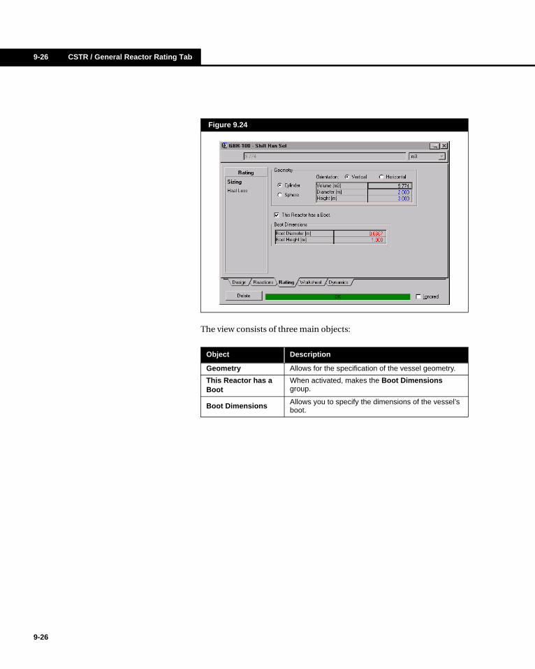
9-26 CSTR / General Reactor Rating Tab
9-26
The view consists of three main objects:
Figure 9.24
Object Description
Geometry Allows for the specification of the vessel geometry.
This Reactor has a Boot
When activated, makes the Boot Dimensions group.
Boot Dimensions Allows you to specify the dimensions of the vessel’s boot.

Reactors 9-27
Geometry Group
This group contains 5 objects which aid in the specification of the vessel volume:
The Geometry group contains three fields: Volume, Diameter and Height (or Length depending on orientation). If you specify the Volume
Object Description
Cylinder / Sphere
Toggles the shape of the vessel between Sphere and Cylinder. This will affect the number of specifications required as well as the method of volume calculation.
If Cylinder is selected and a diameter and height have been specified, the vessel volume will be calculated as:
(9.8)
If Sphere is selected and either the height or diameter have been specified the vessel volume is calculated as:
(9.9)
where: Vreactor = the Volume of the reactor
Vboot = the volume of the boot
Height, Diameter = the values taken from the respective fields
Orientation
You may choose the orientation of the vessel as either:
• Horizontal - the ends of the vessels are horizontally orientated.
• Vertical - the ends of the vessel are vertically orientated.
Volume
Contains the total volume of the vessel.
There are three possibilities for values in this field:
• If the height and/or diameter have been entered, this field will display the value calculated using either Equation (9.8) or Equation (9.9).
• If you enter a value into this field and either the Height (Length) or Diameter is specified, HYSYS will back calculate the other parameter using either Equation (9.8) or Equation (9.9). This is only possible with cylindrical vessels as spherical vessels have the height equal to the diameter.
• If you enter a value into this field (and only this field) both the Height (Length) and Diameter will be calculated assuming a ratio of 3/2 (i.e. Height: Diameter).
Diameter Holds the diameter of the vessel. If the vessel is a Sphere, then it will be the same value as the Height (Length).
Height / LengthHolds the height or length of the vessel depending on the vessels orientation (vertical or horizontal). If the vessel is a Sphere, then it will be the same value as the diameter.
VreactorDiameter
2
4---------------------------π Height×
Vboot+=
VreactorHeight or Diameter( )3π
6---------------------------------------------------------- Vboot+=
9-27

9-28 CSTR / General Reactor Rating Tab
9-28
then you are not required to specify the other two parameters as HYSYS will calculate a Height (or Length) and Diameter assuming a ratio of Height to Diameter of 3/2. You may however specify one of the two parameters (either Height or Diameter) and the third will be automatically calculated using either Equation (9.8) or Equation (9.9).
Boot Dimensions
If the reactor you are rating has a Boot, you may include it’s volume in the total vessel volume by activating the This Reactor has a Boot check box. This will make the Boot Dimensions group box visible. The Boot Dimensions group consists of two fields:
The volume of the boot is calculated using a simple cylindrical volume calculation:
and the default reactor parameters are:
This means that this too can be estimated by just entering the total Reactor volume.
Heat Loss Page
The Heat Loss page allows you to specify which Heat Loss Model you want to implement and to define the parameters associated with each model. For information on specifying information on this page, please see the Dynamics Modelling guide.
Field Description
Boot Diameter This is the diameter of the boot. The default value for this field is usually 1/3 the reactor diameter.
Boot Height This value is the height of the boot which is defaulted at half the reactor diameter.
(9.10)VBoot π Boot Diameter2
----------------------------------- 2
Boot Height×=
(9.11)VBoot π Diameter
6-------------------------
2 Diameter2
-------------------------×=
π Diameter( )3
72------------------------------------=

Reactors 9-29
9.5 CSTR / General Reactor Work Sheet Tab
The Work Sheet tab contains a summary of the information contained in the Stream property view of all the streams attached to the unit operation. The Conditions, Properties, and Composition pages contain selected information from the corresponding pages of the Worksheet tab of the stream property view. The PF Specs page contains a summary of the Stream property view Dynamics tab.
9.6 CSTR / General Reactor Dynamics Tab
If you are working exclusively in Steady State mode, you are not required to change any information on the pages accessible through this tab. For more information on running the CSTR and General Reactors in dynamic mode, see the HYSYS Dynamic Modelling guide.
9.7 Plug Flow Reactor (PFR) Property View
The PFR (Plug Flow Reactor, or Tubular Reactor) generally consists of a bank of cylindrical pipes or tubes. The flow field is modelled as plug flow, implying that the stream is radially isotropic (without mass or energy gradients). This also implies that axial mixing is negligible.
As the reactants flow the length of the reactor, they are continually consumed, hence, there will be an axial variation in concentration. Since reaction rate is a function of concentration, the reaction rate will also vary axially (except for zero-order reactions).
Figure 9.25
9-29

9-30 Plug Flow Reactor (PFR) Property View
9-30
To obtain the solution for the PFR (axial profiles of compositions, temperature, etc.), the reactor is divided into several subvolumes. Within each subvolume, the reaction rate is considered to be spatially uniform. A mole balance is done in each subvolume j:
Because the reaction rate is considered spatially uniform in each subvolume, the third term reduces to rjV. At steady state, the right side of this balance will equal zero, and the equation reduces to:
To install the PFR operation, press F12 and choose Plug Flow Reactor from the Unit Ops view or select the Plug Flow Reactor button in the Object Palette.
9.7.1 PFR Design TabThe Design tab of the PFR consists of five pages:
(9.12)Fj0 Fj– rj VdV
∫+Njd
dt--------=
(9.13)Fj Fj0 rjV+=
PFR Button
Page Input Required
Connections Attaches the feed and product streams to the reactor.
Parameters Allows for the specification of pressure drops and energy streams.
Heat Transfer Allows you to specify the heat transfer parameters.
User Variables Creates user variables for use in this operation as well as several others.
Notes Allows you to add notes to this reactor.

Reactors 9-31
Connections Page
On the Connections page, you may provide the Operation name, as well as the names of the feed(s), product and energy streams. Note that if you do not provide an energy stream, the operation is considered to be adiabatic.
Figure 9.26
Object Input Required
Inlets Where the reactor feed streams are selected.
Outlet Contains the name of the reactor product stream.
Energy (Optional)
As mentioned in the field name, you are not required to provide an energy stream however under those circumstances HYSYS will assume that the operation is adiabatic.
9-31

9-32 Plug Flow Reactor (PFR) Property View
9-32
Parameters Page
The Parameters page is divided into three sections, from which you instruct HYSYS on the calculations for pressure drop and heat transfer and also decide whether the operation will be included in the calculations.
Figure 9.27
To ignore the PFR during calculations, select the Ignore check box. HYSYS will completely disregard the operation until you restore the operation to an active state by clearing the check box.
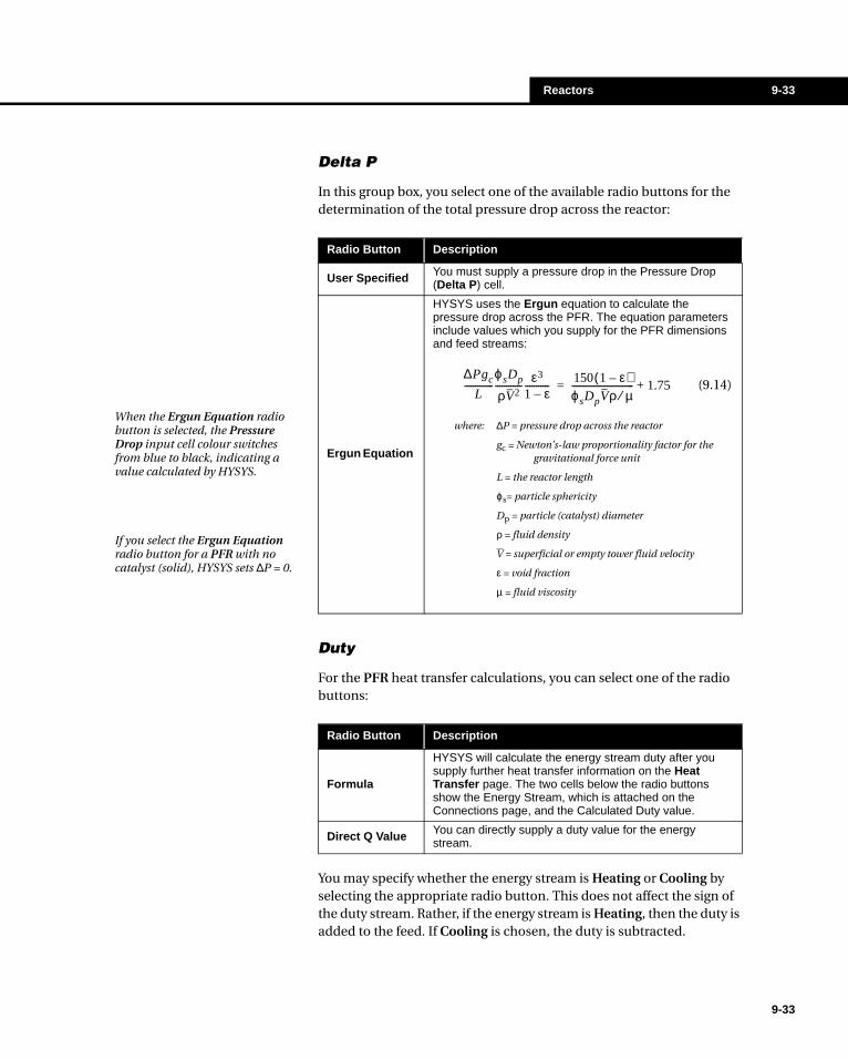
Reactors 9-33
Delta P
In this group box, you select one of the available radio buttons for the determination of the total pressure drop across the reactor:
Duty
For the PFR heat transfer calculations, you can select one of the radio buttons:
You may specify whether the energy stream is Heating or Cooling by selecting the appropriate radio button. This does not affect the sign of the duty stream. Rather, if the energy stream is Heating, then the duty is added to the feed. If Cooling is chosen, the duty is subtracted.
Radio Button Description
User Specified You must supply a pressure drop in the Pressure Drop (Delta P) cell.
Ergun Equation
HYSYS uses the Ergun equation to calculate the pressure drop across the PFR. The equation parameters include values which you supply for the PFR dimensions and feed streams:
(9.14)
where: ∆P = pressure drop across the reactor
gc = Newton’s-law proportionality factor for the gravitational force unit
L = the reactor length
ϕs= particle sphericity
Dp = particle (catalyst) diameter
ρ = fluid density
V = superficial or empty tower fluid velocity
ε = void fraction
µ = fluid viscosity
When the Ergun Equation radio button is selected, the Pressure Drop input cell colour switches from blue to black, indicating a value calculated by HYSYS.
If you select the Ergun Equation radio button for a PFR with no catalyst (solid), HYSYS sets ∆P = 0.
∆Pgc
L-------------
ϕsDp
ρV2------------
ε3
1 ε–-----------
150 1 ε–( )ϕsDpVρ µ⁄---------------------------- 1.75+=
Radio Button Description
Formula
HYSYS will calculate the energy stream duty after you supply further heat transfer information on the Heat Transfer page. The two cells below the radio buttons show the Energy Stream, which is attached on the Connections page, and the Calculated Duty value.
Direct Q Value You can directly supply a duty value for the energy stream.
9-33
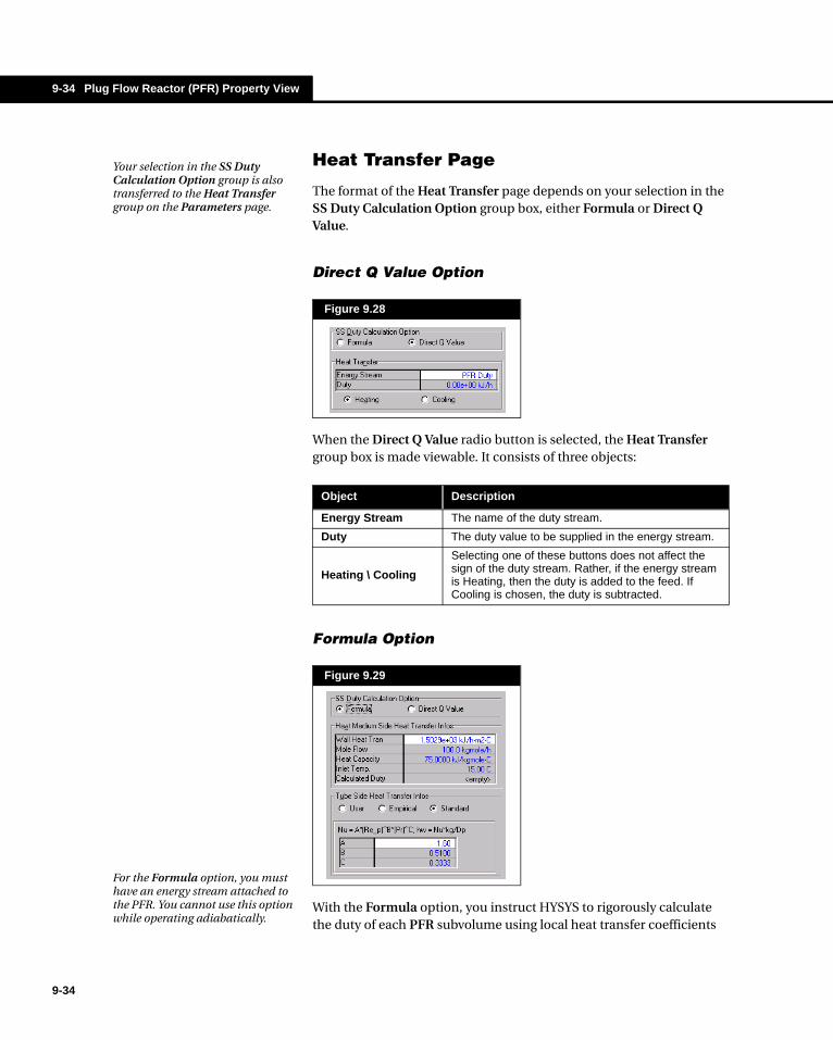
9-34 Plug Flow Reactor (PFR) Property View
9-34
Heat Transfer Page
The format of the Heat Transfer page depends on your selection in the SS Duty Calculation Option group box, either Formula or Direct Q Value.
Direct Q Value Option
When the Direct Q Value radio button is selected, the Heat Transfer group box is made viewable. It consists of three objects:
Formula Option
With the Formula option, you instruct HYSYS to rigorously calculate the duty of each PFR subvolume using local heat transfer coefficients
Figure 9.28
Your selection in the SS Duty Calculation Option group is also transferred to the Heat Transfer group on the Parameters page.
Object Description
Energy Stream The name of the duty stream.
Duty The duty value to be supplied in the energy stream.
Heating \ Cooling
Selecting one of these buttons does not affect the sign of the duty stream. Rather, if the energy stream is Heating, then the duty is added to the feed. If Cooling is chosen, the duty is subtracted.
Figure 9.29
For the Formula option, you must have an energy stream attached to the PFR. You cannot use this option while operating adiabatically.
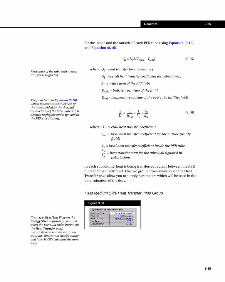
Reactors 9-35
for the inside and the outside of each PFR tube using Equation (9.15) and Equation (9.16).
where: Qj = heat transfer for subvolume j
Uj = overall heat transfer coefficient for subvolume j
A = surface area of the PFR tube
Tbulkj = bulk temperature of the fluid
Toutj = temperature outside of the PFR tube (utility fluid)
where: U = overall heat transfer coefficient
hout = local heat transfer coefficient for the outside (utility fluid)
hw = local heat transfer coefficient inside the PFR tube
= heat transfer term for the tube wall (ignored in calculations)
In each subvolume, heat is being transferred radially between the PFR fluid and the utility fluid. The two group boxes available on the Heat Transfer page allow you to supply parameters which will be used in the determination of the duty.
Heat Medium Side Heat Transfer Infos Group
Qj = UjA(Tbulkj - Toutj) (9.15)
Resistance of the tube wall to heat transfer is neglected.
(9.16)1U----
1hout---------
1hw------
xw
km------+ +=
The final term in Equation (9.16), which represents the thickness of the tube divided by the thermal conductivity of the tube material, is deemed negligible and is ignored in the PFR calculations.
Figure 9.30
xw
km------
If you specify a Heat Flow on the Energy Stream property view and select the Formula radio button on the Heat Transfer page, inconsistencies will appear in the solution. You cannot specify a duty and have HYSYS calculate the same duty.
9-35

9-36 Plug Flow Reactor (PFR) Property View
9-36
In this group, you can modify the parameters which are used to calculate the duty (Qj) for the outside of each PFR subvolume:
The equation used to determine the temperature of the utility fluid entering each subvolume j is:
Tube Side Heat Transfer Info Group
In this group box, you can select the method for determining the inside local heat transfer coefficient (hw) by choosing a radio button and supplying the required parameters:
ParameterFormula Variable
Input Required
Wall Heat Transfer Coefficient
hout
Specify a value for the local heat transfer coefficient. Since the UA value, in this case the U being the local heat transfer coefficient, is constant, changes made to the specified Length, Diameter or Number of Tubes (on the Dimensions page) will affect hout.
Mole Flow m Molar flow of the energy stream utility fluid.
Heat Capacity CpHeat capacity of the energy stream utility fluid.
Inlet Temperature
TThe temperature of the utility fluid entering the PFR.
Calculated Duty
QjDuty calculated for each PFR subvolume.
Qj = mρCp(Tj - Tj+1) (9.17)
Radio Button Description View
User
Supply a value for the local heat transfer coefficient in the User Specified input cell.

Reactors 9-37
User Variables Page
The User Variables page allows you to create and implement variables in the HYSYS simulation case. For more information on implementing the User Variables option, see Chapter 5 - User Variables of the Customization Guide.
Notes Page
The Notes page provides a text editor where you can record any comments or information regarding the PFR or pertaining to the simulation in general.
9.7.2 Reactions TabYou may add a Reaction Set to the PFR on the Reactions tab. Note that only Kinetic, Heterogeneous Catalytic and Simple Rate reactions are allowed in the PFR. The tab consists of three pages: Overall, Details and Results.
Empirical
Supply coefficients for the empirical equation which relates the heat transfer coefficient to the flowrate of the PFR fluid via the following equation:
(9.18)
You can also choose the basis for the equation as Molar, Mass or Volume.
Standard
Supply coefficients for the calculation of the Nusselt number, which is then used to calculate the local heat transfer coefficient:
(9.19)
(9.20)
Radio Button Description View
hw A FlowB×=
Nu A ReB× PrC×=
hw
Nukg
Dp------------=
HYSYS uses the following defaults:
A = 1.6, B = 0.51,C = 0.33
9-37

9-38 Plug Flow Reactor (PFR) Property View
9-38
Overall Page
On this page, the Reaction Set and calculation information are specified. The page is split into three groups: Reaction Info, Integration Information, and Catalyst Data.
Reaction Info Group
In this group box you are required to supply two pieces of information: the Reaction Set to be used and the segment initialization method. The Reaction Set is selected from the aptly named Reaction Set drop down list. Note that the Reaction Set you wish to use must be attached to the Fluid Package you are using in this environment.
As described earlier in this section, the PFR is split into segments by the reactor solver algorithm; HYSYS will obtain a solution in each segment of the reactor. The segment reactions may be initialized using the following methods:
Figure 9.31
Figure 9.32

Reactors 9-39
Integration Information
This group consists of three fields:
During each segment calculation, HYSYS will attempt to calculate a solution over the complete segment length. If a solution cannot be obtained, the current segment will be halved, and HYSYS will attempt to determine a solution over the first half of the segment. The segment will continue to be halved until a solution is obtained, at which point the remaining portion of the segment will be calculated. If the segment is divided to the point where its length is less than the Minimum Step Length, calculations will stop.
Initialization Option Description
Current Initializes from the most recent solution of the current segment.
Previous Initializes from the most recent solution of the previous segment.
Re-init Reinitializes the current segment reaction calculations.
Figure 9.33
Field Description
Number of Segments
The number of segments you want to split the PFR into.
Minimum Step Fraction
The minimum fraction an unresolved segment will split too.
Minimum Step Length
The product of the Reactor Length and the Minimum Step Fraction.
The length of each segment stays constant during the calculations. However, if a solution cannot be obtained for an individual segment, it will be divided into smaller sections until a solution is reached. This does not affect the other segments.
9-39
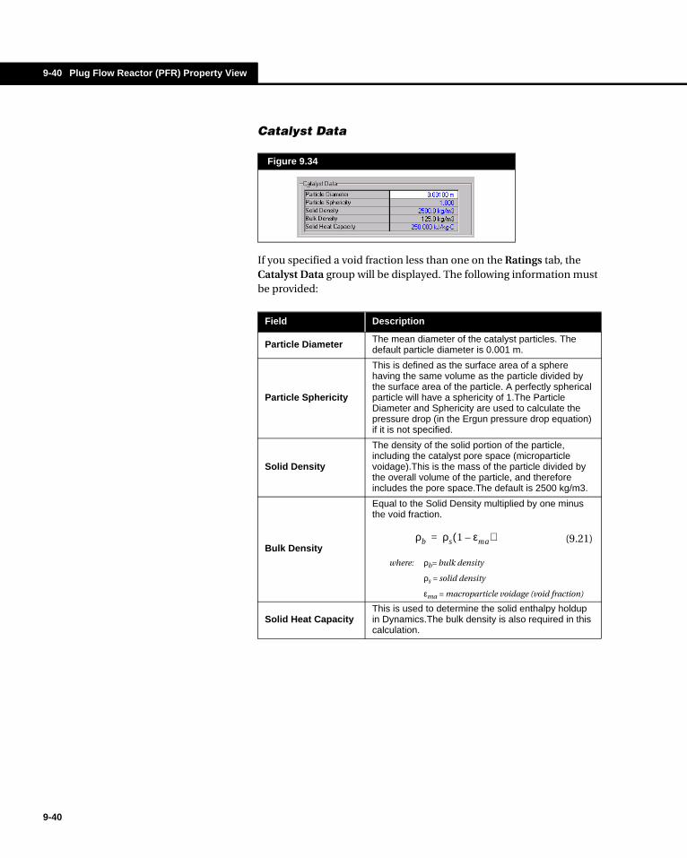
9-40 Plug Flow Reactor (PFR) Property View
9-40
Catalyst Data
If you specified a void fraction less than one on the Ratings tab, the Catalyst Data group will be displayed. The following information must be provided:
Figure 9.34
Field Description
Particle Diameter The mean diameter of the catalyst particles. The default particle diameter is 0.001 m.
Particle Sphericity
This is defined as the surface area of a sphere having the same volume as the particle divided by the surface area of the particle. A perfectly spherical particle will have a sphericity of 1.The Particle Diameter and Sphericity are used to calculate the pressure drop (in the Ergun pressure drop equation) if it is not specified.
Solid Density
The density of the solid portion of the particle, including the catalyst pore space (microparticle voidage).This is the mass of the particle divided by the overall volume of the particle, and therefore includes the pore space.The default is 2500 kg/m3.
Bulk Density
Equal to the Solid Density multiplied by one minus the void fraction.
(9.21)
where: ρb= bulk density
ρs = solid density
εma = macroparticle voidage (void fraction)
Solid Heat CapacityThis is used to determine the solid enthalpy holdup in Dynamics.The bulk density is also required in this calculation.
ρb ρs 1 εma–( )=

Reactors 9-41
Details Page
On this page you can manipulate the Reactions attached to the selected Reactions Set. The page is split into 3 objects:
Figure 9.35
Object Description
ReactionFrom this drop down you must select the appropriate reaction from the Reaction Set selected on the Overall page.
View Reaction
Opens the Reaction property view for the selected Reaction. This allows you to edit the reaction. Editing the Reaction dialogue will effect all other implementations of the particular Reaction.
SpecificsThese radio buttons allow you to toggle between the Stoichiometry group box or the Basis group box. (described in the following subsection)
9-41
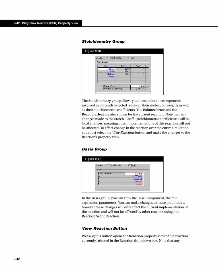
9-42 Plug Flow Reactor (PFR) Property View
9-42
Stoichiometry Group
The Stoichiometry group allows you to examine the components involved in currently selected reaction, their molecular weights as well as their stoichiometric coefficients. The Balance Error and the Reaction Heat are also shown for the current reaction. Note that any changes made to the Stoich. Coeff. (stoichiometric coefficients) will be local changes, meaning other implementations of this reaction will not be affected. To affect change in the reaction over the entire simulation you must select the View Reaction button and make the changes to the Reaction’s property view.
Basis Group
In the Basis group, you can view the Base Component, the rate expression parameters. You can make changes to these parameters, however these changes will only affect the current implementation of the reaction and will not be affected by other reactors using this Reaction Set or Reaction.
View Reaction Button
Pressing this button opens the Reaction property view of the reaction currently selected in the Reaction drop down box. Note that any
Figure 9.36
Figure 9.37
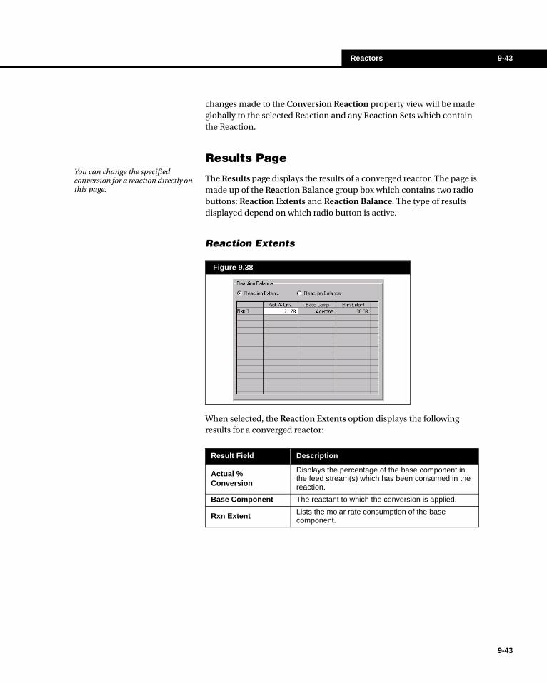
Reactors 9-43
changes made to the Conversion Reaction property view will be made globally to the selected Reaction and any Reaction Sets which contain the Reaction.
Results Page
The Results page displays the results of a converged reactor. The page is made up of the Reaction Balance group box which contains two radio buttons: Reaction Extents and Reaction Balance. The type of results displayed depend on which radio button is active.
Reaction Extents
When selected, the Reaction Extents option displays the following results for a converged reactor:
Figure 9.38
You can change the specified conversion for a reaction directly on this page.
Result Field Description
Actual % Conversion
Displays the percentage of the base component in the feed stream(s) which has been consumed in the reaction.
Base Component The reactant to which the conversion is applied.
Rxn Extent Lists the molar rate consumption of the base component.
9-43

9-44 Plug Flow Reactor (PFR) Property View
9-44
Reaction Balance
When selected the Reaction Balance option provides an overall component summary for the PFR. All components which appear in the fluid package are shown here.
Values appear after all reactions have been completed. The Total Inflow rate, the Total Reacted rate and the Total Outflow rate for each component are provided on a molar basis. Negative values indicate the consumption of a reactant, while positive values indicate the appearance of a product.
Figure 9.39Any changes made to the global reaction will affect all reaction sets to which the reaction is attached, provided local changes have not been made.

Reactors 9-45
9.7.3 Ratings TabThe Ratings tab contains one page: Sizing.
Sizing Page
On the Sizing page, you can specify the Tube Dimensions and the Tube Packing information in their respective groups.
Tube Dimensions
For the tube dimensions, you will need to specify any three of the following four parameters:
When three of these dimensions are specified, the fourth will automatically be calculated. Note that the Total Volume refers to the combined volumes of all tubes.
Figure 9.40
Tube Dimension Description
Total Volume Total volume of the PFR.
Length The total length of the individual tube.
Diameter The diameter of an individual tube.
Number of tubes. The total number of tubes required. This will always be calculated to the nearest integer value.
9-45

9-46 Plug Flow Reactor (PFR) Property View
9-46
By default, the number of tubes is set to 1. Although the number of tubes is generally specified, you may set this parameter as a calculated value by selecting the Number of Tubes field and pressing the DELETE key. The number of tubes will always be calculated as an integer value. It is possible to obtain a rounded value of 0 as the number of tubes, depending on what you specified for the tube dimensions. In this case, you will have to re-specify the tube dimensions.
The Tube Wall Thickness may also be specified.
Tube Packing
This group consists of two fields: Void Fraction and Void Volume. The Void Fraction is by default set to 1, in which case there is no catalyst present in the reactor. The resulting Void Volume will be equal to the reactor volume.
At Void Fractions less than 1, the Void Volume is the product of the Total Volume and Void Fraction. In this case, you will also be required to provide information on the Overall page of the Reactions tab. This information is used to calculate pressure drop, reactor heat capacity and spatial velocity of the fluid travelling down the reactor.
9.7.4 Work Sheet TabThe Worksheet tab contains a summary of the information contained in the Stream property view for all the streams attached in the unit operation. The Conditions, Properties, and Compositions pages contain selected information from the corresponding pages of the Worksheet tab for the Stream property view. The PF Specs page contains a summary of the Stream property view Dynamics tab.
The Void Volume is used to calculate the spatial velocity, which impacts the rate of reaction.
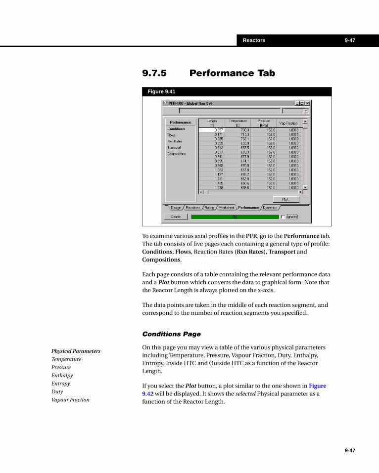
Reactors 9-47
9.7.5 Performance Tab
To examine various axial profiles in the PFR, go to the Performance tab. The tab consists of five pages each containing a general type of profile: Conditions, Flows, Reaction Rates (Rxn Rates), Transport and Compositions.
Each page consists of a table containing the relevant performance data and a Plot button which converts the data to graphical form. Note that the Reactor Length is always plotted on the x-axis.
The data points are taken in the middle of each reaction segment, and correspond to the number of reaction segments you specified.
Conditions Page
On this page you may view a table of the various physical parameters including Temperature, Pressure, Vapour Fraction, Duty, Enthalpy, Entropy, Inside HTC and Outside HTC as a function of the Reactor Length.
If you select the Plot button, a plot similar to the one shown in Figure 9.42 will be displayed. It shows the selected Physical parameter as a function of the Reactor Length.
Figure 9.41
Physical Parameters
Temperature
Pressure
Enthalpy
Entropy
Duty
Vapour Fraction
9-47
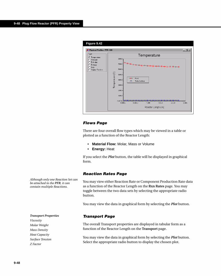
9-48 Plug Flow Reactor (PFR) Property View
9-48
Flows Page
There are four overall flow types which may be viewed in a table or plotted as a function of the Reactor Length:
• Material Flow: Molar, Mass or Volume• Energy: Heat
If you select the Plot button, the table will be displayed in graphical form.
Reaction Rates Page
You may view either Reaction Rate or Component Production Rate data as a function of the Reactor Length on the Rxn Rates page. You may toggle between the two data sets by selecting the appropriate radio button.
You may view the data in graphical form by selecting the Plot button.
Transport Page
The overall Transport properties are displayed in tabular form as a function of the Reactor Length on the Transport page.
You may view the data in graphical form by selecting the Plot button. Select the appropriate radio button to display the chosen plot.
Figure 9.42
Although only one Reaction Set can be attached to the PFR, it can contain multiple Reactions.
Transport Properties
Viscosity
Molar Weight
Mass Density
Heat Capacity
Surface Tension
Z Factor
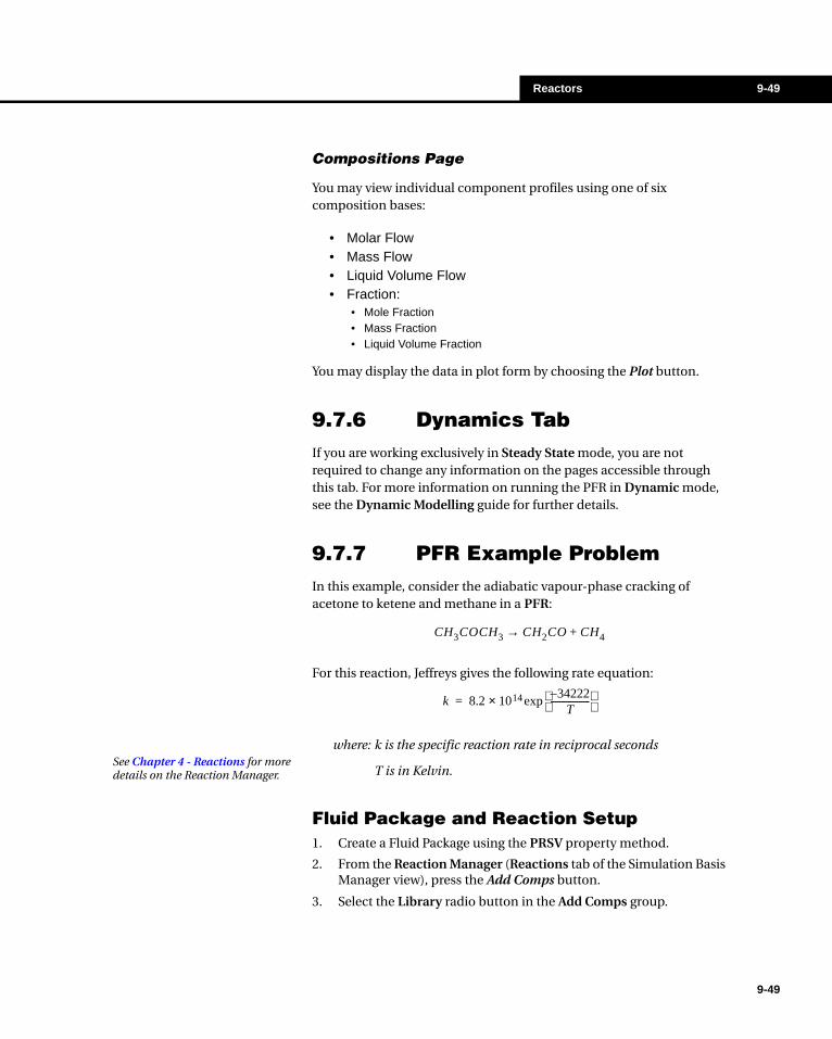
Reactors 9-49
Compositions Page
You may view individual component profiles using one of six composition bases:
• Molar Flow• Mass Flow• Liquid Volume Flow• Fraction:
• Mole Fraction• Mass Fraction• Liquid Volume Fraction
You may display the data in plot form by choosing the Plot button.
9.7.6 Dynamics TabIf you are working exclusively in Steady State mode, you are not required to change any information on the pages accessible through this tab. For more information on running the PFR in Dynamic mode, see the Dynamic Modelling guide for further details.
9.7.7 PFR Example ProblemIn this example, consider the adiabatic vapour-phase cracking of acetone to ketene and methane in a PFR:
For this reaction, Jeffreys gives the following rate equation:
where: k is the specific reaction rate in reciprocal seconds
T is in Kelvin.
Fluid Package and Reaction Setup1. Create a Fluid Package using the PRSV property method.
2. From the Reaction Manager (Reactions tab of the Simulation Basis Manager view), press the Add Comps button.
3. Select the Library radio button in the Add Comps group.
CH3COCH3 CH2CO CH4+→
k 8.2 1014 34222–T
------------------ exp×=
See Chapter 4 - Reactions for more details on the Reaction Manager.
9-49

9-50 Plug Flow Reactor (PFR) Property View
9-50
4. Choose Acetone, Methane and Ketene as the components for the example.
5. Close the Reaction Component Selection view.
6. After returning to the Reaction Manager, press the Add Reaction button.
7. Highlight Kinetic in the Reactions view and press the Add Reaction button. The Kinetic Reaction property view will appear.
8. Complete the Stoichiometry, Basis and Parameters tabs as shown below:
Since there is only one reaction being used, we can use the Global Rxn Set. The reaction is automatically attached in this set.
Now you must attach the reaction components to the Fluid Package and make the reaction set available in the Main Flowsheet. This can be done from the Reaction Manager view:
1. Highlight the Global Rxn Set in the Reaction Sets group.
2. Press the Add to FP button.
The Reverse Orders are not required for this reaction, but are automatically provided when you enter the stoichiometric coefficient.
Since reverse reaction information is not supplied, the Reverse Orders are ignored.
Figure 9.43
The value of A was taken directly from the given rate equation, but a calculation was needed to obtain E. It can be seen that E/R = 34222 (units K). Therefore, E = 34222R and R must be chosen such that temperature units are obtained for the constant value. Use R = 8.31 kJ/kmol K, obtaining E = 2.85 x 10⁵ kJ/kmol.
The general Kinetic expression is:
k AeE
RT-------–
=
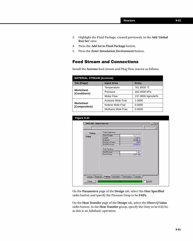
Reactors 9-51
3. Highlight the Fluid Package, created previously, in the Add ’Global Rxn Set’ view.
4. Press the Add Set to Fluid Package button.
5. Press the Enter Simulation Environment button.
Feed Stream and Connections
Install the Acetone feed stream and Plug Flow reactor as follows:
On the Parameters page of the Design tab, select the User Specified radio button and specify the Pressure Drop to be 0 kPa.
On the Heat Transfer page of the Design tab, select the Direct Q Value radio button. In the Heat Transfer group, specify the Duty to be 0 kJ/hr, as this is an Adiabatic operation.
MATERIAL STREAM [Acetone]
Tab [Page] Input Area Entry
Worksheet [Conditions]
Temperature 761.8500 °C
Pressure 162.0000 kPa
Molar Flow 137.9000 kgmole/hr
Worksheet [Composition]
Acetone Mole Frac 1.0000
Ketene Mole Frac 0.0000
Methane Mole Frac 0.0000
Figure 9.44
9-51

9-52 Plug Flow Reactor (PFR) Property View
9-52
Rating Tab
Complete the Tube Dimensions and Tube Packing as shown in Figure 9.45. Only specify the Tube Volume, Length, Number of Tubes, Wall Thickness and Void Fraction (Total Volume will be calculated). The Diameter of the tubes will be calculated.
Consider a reactor consisting of a bank of one thousand 1-in. schedule 40 tubes, 2.28 m in length. The internal diameter of 1-in. schedule pipe is 1.049" (0.0266 m) and the wall thickness is 0.133" (0.0034 m). Use a void fraction of 1.
Reactions Tab
On the Overall page of the Reactions tab, attach the Global Rxn Set to the PFR. It is not necessary to change the Integration Information from the default values. The Reactor should immediately begin solving.
Because the void fraction is specified as 1, you are not required to input any catalyst information. In essence, you have indicated that no catalyst is present.
Figure 9.45

Reactors 9-53
Steady State Solution and Profiles
HYSYS will now converge to a Steady State Solution. Watch the Status Line at the bottom of the property view, and observe the temperature. The solution will converge when the temperature reaches about 664oC. The product stream (PFR Product) specs are shown below.
You may view various reactor profiles by going to the Performance tab and pressing the Plot button. The axial temperature profile will initially be displayed. You can select other profiles on the Conditions page by choosing a different radio button in the Type group.
Select any of the five pages to view other PFR data, either in graphical or tabular form.
Name PFR Product
Vapour Frac 1.0000
Temperature [C] 649.0101
Pressure [kPa] 162.0000
Molar Flow [kgmole/hr] 167.9292
Mass Flow [kg/hr] 8009.2488
Liq Vol Flow [m3/day] 11.3991
Heat Flow [kJ/hr] -1.7157e+07
Comp Mole Frac [Methane] 0.6424
Comp Mole Frac [Acetone] 0.1788
Comp Mole Frac [Ketene] 0.1788
Figure 9.46
Object inspect the plot area and select Graph Control to access the graph editing options. Refer to Section 6.4 - Graph Control for more information.
9-53

9-54 Plug Flow Reactor (PFR) Property View
9-54
Logical Operations 10-1
10 Logical Operations
10.1 Adjust .......................................................................................................... 3
10.1.1 Connections Tab .................................................................................... 410.1.2 Parameters Tab...................................................................................... 610.1.3 Monitor Tab ...........................................................................................1110.1.4 Starting the Adjust................................................................................ 1210.1.5 Individual ADJUST............................................................................... 1310.1.6 Multiple ADJUST.................................................................................. 16
10.2 Balance...................................................................................................... 17
10.2.1 Connections Tab .................................................................................. 1810.2.2 Parameters Tab.................................................................................... 1910.2.3 Mole and Heat Balance........................................................................ 1910.2.4 Mole Balance ....................................................................................... 2310.2.5 Mass Balance ...................................................................................... 2510.2.6 Heat Balance ....................................................................................... 2710.2.7 General Balance .................................................................................. 29
10.3 Parametric Unit Operation....................................................................... 34
10.3.1 Design Tab ........................................................................................... 3410.3.2 Parameters Tab.................................................................................... 3910.3.3 Worksheet Tab ..................................................................................... 41
10.4 Recycle...................................................................................................... 42
10.4.1 Connections Tab .................................................................................. 4310.4.2 Parameters Tab.................................................................................... 4410.4.3 Worksheet Tab ..................................................................................... 4910.4.4 Monitor Tab .......................................................................................... 5010.4.5 Calculations ......................................................................................... 5110.4.6 Reducing Convergence Time............................................................... 5110.4.7 Single Recycle Example ...................................................................... 52
10-1
10-2
10-2
10.4.8 Multiple Recycle Example.................................................................... 5610.4.9 Multiple Recycle Example Revisited .................................................... 61
10.5 Set.............................................................................................................. 64
10.5.1 Connections Tab .................................................................................. 6510.5.2 Parameters Tab.................................................................................... 6610.5.3 Set Example......................................................................................... 66
10.6 Spreadsheet.............................................................................................. 69
10.6.1 Spreadsheet Functions ........................................................................ 7110.6.2 Spreadsheet Interface.......................................................................... 7510.6.3 Spreadsheet Tabs ................................................................................ 7910.6.4 Spreadsheet Example.......................................................................... 85
Logical Operations 10-3
10.1 AdjustThe ADJUST operation will vary the value of one stream variable (the independent variable) to meet a required value or specification (the dependent variable) in another stream or operation.
In a Flowsheet, a certain combination of specifications may be required which cannot be solved directly. These types of problems must be solved using trial-and-error techniques. To quickly solve Flowsheet problems that fall into this category, the ADJUST operation can be used to automatically conduct the trial-and-error iterations for you.
The ADJUST is extremely flexible. It allows you to link stream variables in the Flowsheet in ways that are not possible using ordinary "physical" unit operations. It can be used to solve for the desired value of just a single dependent variable, or multiple ADJUSTS can be installed to solve for the desired values of several variables simultaneously.
The ADJUST can perform the following functions:
• Adjust the independent variable until the dependent variable meets the Target Value.
• Adjust the independent variable until the dependent variable equals the value of the same variable for another Object, plus an optional offset.
To install the ADJUST operation, choose Add Operation from the Flowsheet Menu, and select Adjust. Alternatively, select the Adjust button in the Object Palette.
The ADJUST is a steady-state operation; HYSYS ignores it in dynamic mode.
The Independent variable cannot be a calculated value; it must be specified.
Adjust Button
10-3
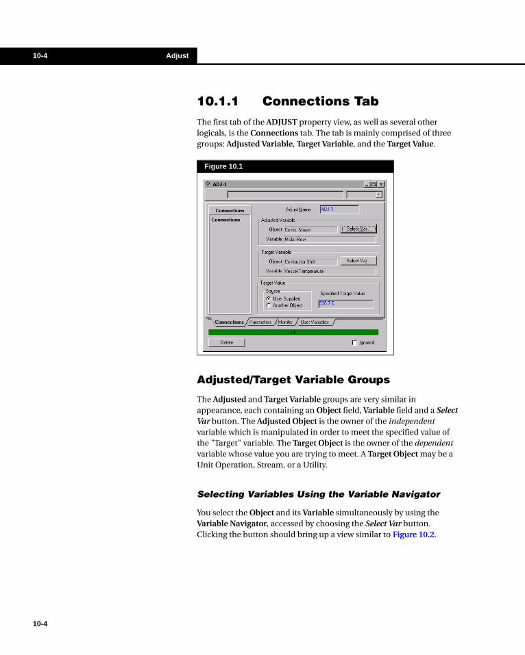
10-4 Adjust
10-4
10.1.1 Connections TabThe first tab of the ADJUST property view, as well as several other logicals, is the Connections tab. The tab is mainly comprised of three groups: Adjusted Variable, Target Variable, and the Target Value.
Adjusted/Target Variable Groups
The Adjusted and Target Variable groups are very similar in appearance, each containing an Object field, Variable field and a Select Var button. The Adjusted Object is the owner of the independent variable which is manipulated in order to meet the specified value of the "Target" variable. The Target Object is the owner of the dependent variable whose value you are trying to meet. A Target Object may be a Unit Operation, Stream, or a Utility.
Selecting Variables Using the Variable Navigator
You select the Object and its Variable simultaneously by using the Variable Navigator, accessed by choosing the Select Var button. Clicking the button should bring up a view similar to Figure 10.2.
Figure 10.1
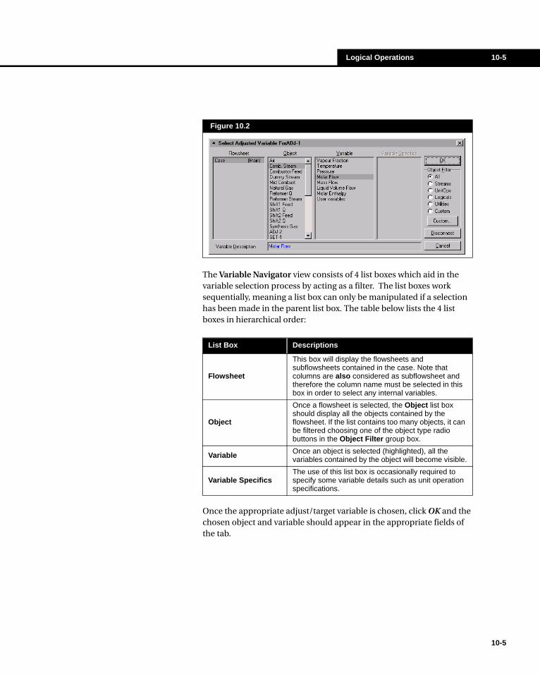
Logical Operations 10-5
The Variable Navigator view consists of 4 list boxes which aid in the variable selection process by acting as a filter. The list boxes work sequentially, meaning a list box can only be manipulated if a selection has been made in the parent list box. The table below lists the 4 list boxes in hierarchical order:
Once the appropriate adjust/target variable is chosen, click OK and the chosen object and variable should appear in the appropriate fields of the tab.
Figure 10.2
List Box Descriptions
Flowsheet
This box will display the flowsheets and subflowsheets contained in the case. Note that columns are also considered as subflowsheet and therefore the column name must be selected in this box in order to select any internal variables.
Object
Once a flowsheet is selected, the Object list box should display all the objects contained by the flowsheet. If the list contains too many objects, it can be filtered choosing one of the object type radio buttons in the Object Filter group box.
Variable Once an object is selected (highlighted), all the variables contained by the object will become visible.
Variable SpecificsThe use of this list box is occasionally required to specify some variable details such as unit operation specifications.
10-5

10-6 Adjust
10-6
Target Value
Once the Target Object and Variable are defined, there are two choices for how the Target is to be satisfied:
• If the Target Variable is to meet a certain numerical value, choose the User Supplied radio button (as shown in Figure 10.1), and enter the appropriate value in the Specified Target Value cell.
• If the Target Variable is to meet the value (or the value plus an offset) of the same variable in another stream or operation, choose the Another Object radio button (as shown below), and select the stream or operation of interest as the Matching Value Object . If applicable, enter an offset in the available field.
10.1.2 Parameters Tab
Figure 10.3
Figure 10.4

Logical Operations 10-7
Once you have chosen the dependent and independent variables, the convergence criteria must be defined. This is usually done in the Parameters tab.
Choosing the Solving Methods
Adjust loops can be solved either individually or simultaneously. If the loop is solved individually, you have the choice of either a Secant (slow and sure) or Broyden (fast but not as reliable) search algorithm. The Simultaneous solution method uses a multiple-variable Broyden search algorithm. A single adjust loop can be solved in the Simultaneous mode, however, this method is usually reserved for multiple inter-linked loops.
When the Simultaneous Solution check box is activated the Method field is no longer visible.
Solving Parameter Description
Simultaneous Solution
Solves multiple ADJUST loops simultaneously. There is only one simultaneous solving method available therefore when this option is activated the Method cell is no longer visible.
Method Sets the (non-simultaneous) solving method: Secant or Broyden.
Tolerance Sets the absolute error. In other words, the maximum difference between the Target Variable and the Target Value.
Step Size The initial step size employed until the solution is bracketed.
Maximum / Minimum The upper and lower bounds for the independent variable (optional) are set in this field.
Maximum Iterations The number of iterations before HYSYS quits calculations, assuming a solution has not been obtained.
Sim Adj ManagerOpens the Simultaneous Adjust Manager allowing you to monitor and modify all adjusts that are selected as simultaneous.
Optimizer Controlled
Passes a variable and a constant to the optimizer. When activated the efficiency of the simultaneous adjust is increased. This option requires RTO.
Figure 10.5
The Calculation Level for an ADJUST (accessed under Main Properties) is 3500, compared to 500 for most streams and operations. This means that the ADJUST will be solved last among unknown operations. You may set the relative solving order of the ADJUSTS by modifying the Calculation Level.
10-7

10-8 Adjust
10-8
Simultaneous Adjust Manager
The Simultaneous Adjust Manager (SAM) allows you to monitor and modify all adjusts that are selected as simultaneous. This gives you access to a more efficient method of calculation and more control over the calculations.
The SAM is launched by clicking the Sim Adj Manager button or by selecting Simultaneous Adjust Manager from the Simulation menu.
The SAM consists of three tabs: Configuration, Parameters and History, together with Stop and Start buttons. The ignored check box switched the SAM off as well as all of the adjusts selected as simultaneous.
Configuration Tab
The Configuration tab displays information regarding adjusts that have been selected as simultaneous. You can view the individual adjusts by double clicking on the adjust name. You can also modify the target value or matching value object, value and offset. This tab also allows you to ignore individual adjusts.
The SAM requires two or more active (i.e. not ignored) adjusts to solve. If you are using only one adjust we recommend using Secant or Broyden modes.
All adjusts in old cases are automatically added to the SAM.
Figure 10.6

Logical Operations 10-9
Parameters Tab
The Parameters tab allows you to modify the tolerance, step size, max and min values for each adjust as well as displays the residual, number of iterations the SAM has taken and the iteration status. This tab also allows you to specify some of the calculation parameters.
History Tab
The History tab displays the Target value, Adjusted value, and Residual value for each iteration of the selected adjust(s). One or more adjusts can be displayed by clicking on the check-box beside the adjust name. The adjusts are always viewed in order from left to right across the page. For example if you are viewing adjust 2 and add adjust 1 to the view, adjust 1 will become the first set of numbers and adjust 2 will be shifted to the right.
Parameter Description
Type of Jacobian Calculation
Allows you to select one of three Jacobian calculations.
• ResetJac - Jacobian is fully calculated and values reset to initial values after each jacobian calculation step. Most time consuming but most accurate.
• Continuous - values are not recalculated between Jacobian calculation steps. Quickest, but allows for “drift” in the Jacobian therefore not as accurate.
• Hybrid - hybrid of the above two methods.
Type of Convergence
Allows you to select one of three convergence types.
• Specified - SAM is converged when all adjusts are within the specified tolerances.
• Norm - SAM is converged when the norm of the residuals (sums of squares) is less then a user specified value.
• Either - SAM is converged with which ever of the above types occurs first.
Max Step Fraction This number x step size is the maximum that the solver is allowed to move during a solve step.
Perturbation Factor
This number x range (Max - Min) or this number x 100 x step size (if no valid range). This is the maximum that the solver is allowed to move during a jacobian step.
Max # of Iterations Maximum number of iterations for the SAM.
This tab only displays the values from a solve step. The values calculated during a jacobian step can be seen on the monitor tab of the adjust for the individual results.
10-9
10-10 Adjust
10-10
Tolerance
For the ADJUST to converge, the error in the dependent variable must be less than the Tolerance.
It is sometimes a good idea to use a relatively loose (large) tolerance when initially attempting to solve an ADJUST loop. Once you determine that everything is working properly, you can reset the tolerance to the final design value. Note that the tolerance and error values are absolute (with the same units as the dependent variable) rather than relative or percentage-type.
Step Size
The step size you enter is used by the search algorithm to establish the maximum step size adjustment applied to the independent variable. This value will be used until the solution has been bracketed, at which time a different convergence algorithm is applied. The value which is supplied should be large enough to permit the solution area to be reached rapidly, but not so large as to result in an unreasonable overshoot into an infeasible region. A positive step size will initially increment the independent variable, while a negative value will initially decrement the independent variable. If the ADJUST steps away from the solution, the direction of the steps will automatically be reversed.
Maximum/Minimum
These two optional criteria are the allowable upper and lower bounds for the independent variable. If either bound is encountered, the ADJUST will stop its search at that point.
(10.1)Error Dependent Variable Value Target Value–=
A negative initial step size causes the first step to decrement the independent variable.
Before installing the ADJUST module, it is often a good practice to initialize the independent variable, and perform one adjust "manually". Solve your Flowsheet once, and note the value for the dependent variable, then self-adjust the independent variable and re-solve the Flowsheet. This assures you that one variable actually affects the other, and also gives you a feel for the step size you need to specify.
The Independent variable must be initialized (have a starting value) in order for the ADJUST to work.

Logical Operations 10-11
Maximum Iterations
The default maximum number of iterations is 10. Should the ADJUST reach this many iterations before converging, the calculations will stop, and you will be asked if you want to continue with more iterations. You may enter any value for the number of maximum iterations.
10.1.3 Monitor Tab
Tables Page
For each Iteration of the ADJUST, the Number, Adjusted Value and Target Value are displayed. If necessary, use the scroll bar to view iterations which are not currently visible.
Figure 10.7
You can also use the Solver Trace Window to view the Iteration History (See Section 5.4 - Object Status Window/Trace Window of the User’s Guide for more information).
Iteration number
Dependent (Target) Variable
Independent (Adjusted) Variable
10-11

10-12 Adjust
10-12
Plots Page
The Plots page displays the Target and Adjusted Variables like on the Tables page, except the information is presented in graph form.
10.1.4 Starting the AdjustThere are two ways to start the ADJUST:
1. If you have provided values for all the fields of the Parameters tab, the ADJUST will automatically begin its calculations.
2. If you have omitted one or both value in the Minimum/Maximum fields (of the Parameters tab) for the independent variable (which are optional Parameters) and you would like the ADJUST to start calculating, simply press the Start button.
The Start button will then change to a red box, indicating the progress of the calculations. The box initially indicates that calculations are "Not Solved"; when the error is less than the tolerance, the status box will display a green "OK" message. If the ADJUST reaches the maximum number of iterations without converging, a red "Reached iteration Limit without converging" message is displayed.
If you press Start when all of the required Parameters are not defined, the yellow status box will display the "Incomplete" message, and calculations will not begin.
Figure 10.8Refer to Section 6.4 - Graph Control for information on customizing plots.
With the exception of the Minimum and Maximum values of the independent (adjusted) variable, all Parameters are required before the ADJUST will begin calculations.

Logical Operations 10-13
Once calculations are underway, you may view the progress of the convergence process by moving to the Iterations tab.
10.1.5 Individual ADJUSTThe Individual ADJUST algorithm, either Secant or Broyden, uses a step-wise trial-and-error method and displays values for the dependent and independent variables on each trial. The step size supplied on the Parameters tab is used to increment or decrement the independent variable for its initial step. The algorithm will continue to use steps of this size until the solution is bracketed. At this point, the algorithm uses either the Secant search (and its own step sizes) or Broyden search, depending on your choice, to quickly converge to the desired value. If a solution has not been reached in the maximum number of iterations, the routine will pause and ask whether another series of trials should be attempted. This is repeated until either a solution is reached or you abandon the search. The Secant search algorithm generally results in good convergence once the solution has been bracketed.
Example
The following will illustrate a simple application of the ADJUST using the Secant algorithm. Stream Feed is fed to a separator (V-100) to produce streams SepLiq and SepVap. The ADJUST is used to vary the temperature of stream Feed until the flow of SepLiq is 100 lbmoles/hr.
To begin, open a new case with Peng Robinson as the Property Package and the following components: Methane, Ethane, Propane, i-Butane, n-Butane, i-Pentane, n-Pentane, n-Hexane, n-Heptane and n-Octane.
Create the following stream Feed.
The Start button only appears in the initialization stage of the ADJUST operation. It disappears from the property view as soon as it is pressed. Any changes made to the ADJUST or other parts the flowsheet will automatically trigger the ADJUST calculation.
To stop or disable the ADJUST activate the Ignored check box.
Note that the feed stream has a specified temperature of 60 °F. The independent variable must be a specified value for the ADJUST to manipulate it.
10-13

10-14 Adjust
10-14
Streams
Install a separator V-100 so that the Connections page of the Design tab match Figure 10.9. Ignore the rest of the tabs as they will not be needed for this example.
MATERIAL STREAM (Feed)
Tab [Page] Input Area Entry
Worksheet [Conditions]
Temperature 60.0000 °F
Pressure 600.0000 psi
Molar Flow 144.0000 lbmole/hr
Worksheet [Composition]
Methane Mole Frac 0.4861
Ethane Mole Frac 0.1389
Propane Mole Frac 0.0694
i-Butane Mole Frac 0.0625
n-Butane Mole Frac 0.0556
i-Pentane Mole Frac 0.0486
n-Pentane Mole Frac 0.0417
n-Hexane Mole Frac 0.0486
n-Heptane Mole Frac 0.0278
n-Octane Mole Frac 0.0208
Figure 10.9
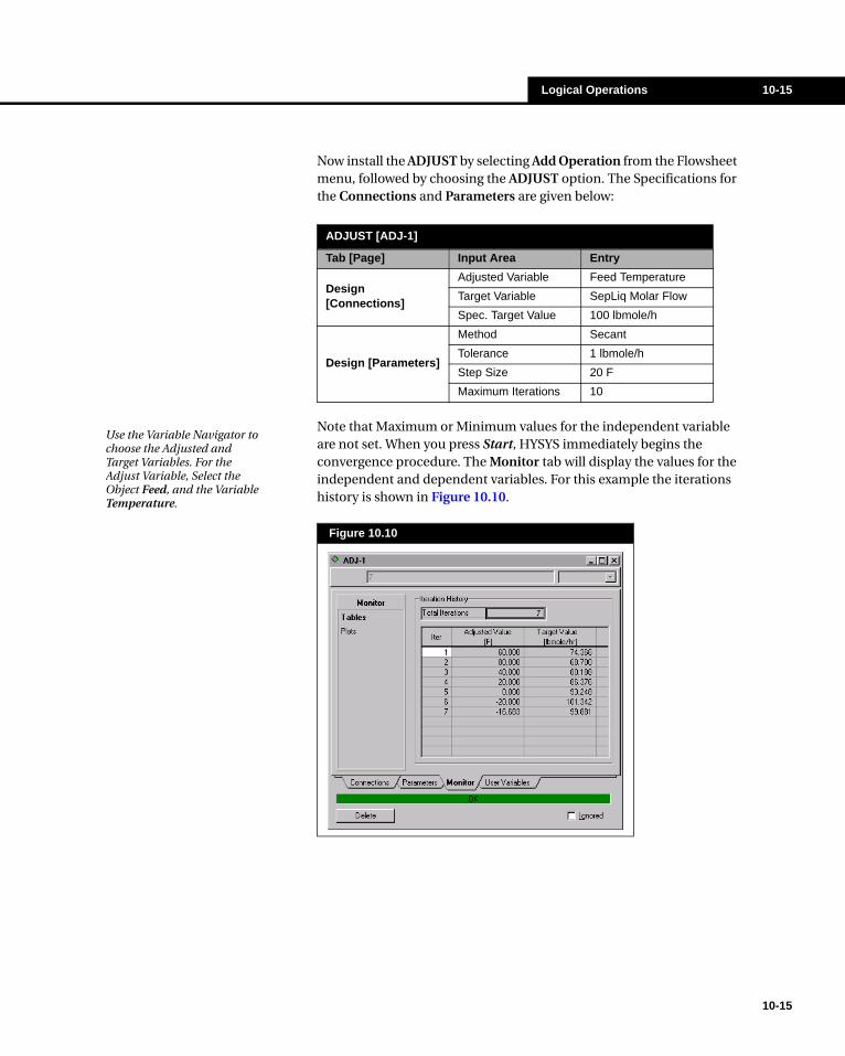
Logical Operations 10-15
Now install the ADJUST by selecting Add Operation from the Flowsheet menu, followed by choosing the ADJUST option. The Specifications for the Connections and Parameters are given below:
Note that Maximum or Minimum values for the independent variable are not set. When you press Start, HYSYS immediately begins the convergence procedure. The Monitor tab will display the values for the independent and dependent variables. For this example the iterations history is shown in Figure 10.10.
ADJUST [ADJ-1]
Tab [Page] Input Area Entry
Design [Connections]
Adjusted Variable Feed Temperature
Target Variable SepLiq Molar Flow
Spec. Target Value 100 lbmole/h
Design [Parameters]
Method Secant
Tolerance 1 lbmole/h
Step Size 20 F
Maximum Iterations 10
Figure 10.10
Use the Variable Navigator to choose the Adjusted and Target Variables. For the Adjust Variable, Select the Object Feed, and the Variable Temperature.
10-15

10-16 Adjust
10-16
The ADJUST converges to the required flow in seven iterations. The new stream conditions are shown in the following table.
Note that the temperature of Feed shows the converged value of -16.68°F in bold typeface (i.e. as a specified value). Although the value which had originally been specified was 60°F, the ADJUST causes the converged solution for the independent variable to become a specified value. If you delete the ADJUST, the new values remain in the Flowsheet.
10.1.6 Multiple ADJUSTThe term Multiple ADJUST typically applies to the situation where all of the ADJUSTS are to be solved simultaneously. In this case, where the results of one ADJUST directly affect the other(s), you can use the Simultaneous option to minimize the number of Flowsheet iterations.
Examples where this feature is very valuable include calculating the flow distribution of pipeline looping networks, or in solving a complex network of UA-constrained heat exchangers. In these examples, you must select the stream parameters which HYSYS is to manipulate to meet the desired specifications. For a pipeline looping problem, the solution may be found by adjusting the flows in the branched streams until the correct pressures are achieved in the pipelines downstream. In any event, it will be up to you to select the variables to adjust to solve your Flowsheet problem.
HYSYS uses a Broyden type search algorithm to simultaneously vary all of the adjustable parameters defined in the Adjusts until the desired specifications are met. The role of step size with this method is quite different. With the single Adjust algorithm, step size is a fixed value used to successively adjust the independent variable until the solution
STREAM
Name Feed
Vapour Frac 0.3064
Temperature [F] -16.68
Pressure [psia] 600.00
Molar Flow [lbmole/hr] 144.
Mass Flow [lb/hr] 5438
Liq Vol Flow [barrel/day]
788.6
Heat Flow [Btu/hr] -7.321e+06
See the Looped Pipeline Example in the Applications guide for an example using Multiple ADJUSTS.
Logical Operations 10-17
has been bracketed. With the simultaneous algorithm, the step size for each variable serves as an upper limit for the adjustment of that variable.
In solving multiple UA exchangers, the starting point should not be one that contains a temperature crossover for one of the heat exchangers. If this occurs, a warning message will appear informing you that a temperature crossover exists (see Section 3.3 - Heat Exchanger), and a very large UA value will be computed for that heat exchanger. This value will be insensitive to any initial change in the value of the adjustable variable, and therefore the matrix cannot be solved.
Install all ADJUSTS using the simultaneous option (Parameters tab, Simultaneous), then press Start to begin the calculations.
10.2 BalanceThe BALANCE operation provides a general-purpose heat and material balance facility. The only information required by the BALANCE is the names of the streams entering and leaving the operation. For the General BALANCE, component ratios can also be specified.
Since HYSYS permits streams to enter or leave more than one operation, the BALANCE can be used in parallel with other units for overall material and energy balances. The BALANCE Operation will solve in both the forward and backward directions. For instance, it will back out the flowrate of an unknown feed, given that there are no degrees of freedom.
There are five BALANCE Types:
One requirement in implementing the Multiple ADJUST feature is that you must start from a feasible solution.
The BALANCE overrides the filtering of streams that HYSYS typically performs.
Balance Type Definition
Mole
An overall balance is performed where only the molar flow of each component is conserved. It can be used to provide material balance envelopes in the Flowsheet or to transfer the flow and composition of a process stream into a second stream.
Mass
An overall balance is performed where only the mass flow is conserved. A common application would be for modelling reactors with no known stoichiometry, but for which analyses of all feeds and products are known.
Heat An overall balance is performed where only the heat flow is conserved. An application would be to provide the pure energy difference in a heat balance envelope.
10-17

10-18 Balance
10-18
To add a BALANCE Operation, choose Add Operation from the Flowsheet menu and select Balance. Alternatively, you may also select the Balance button in the Object Palette.
10.2.1 Connections TabThe Connections tabs is the same for all of the Balance Types.
Mole and Heat
An overall balance is performed where the heat and molar flow is conserved. The most common application for this unit operation would be to perform overall material (molar basis) and energy balance calculations of selected process streams to either check for balances or force HYSYS to calculate an unknown variable, such as flow. Note that most of the unit operations in HYSYS perform the equivalent of a Mole and Heat Balance besides their other more specialized calculations.
General
HYSYS will solve a set of n unknowns in the n equations developed from the streams attached to the operation. Component ratios may be specified on a mole, mass or liquid volume basis.
Balance Type Definition
Most operations in HYSYS perform a Heat and Material Balance as part of their solution.
Figure 10.11
Balance Button

Logical Operations 10-19
On the Connections tab, you must provide the following information:
10.2.2 Parameters TabThe Parameters tab contains two group boxes: Balance Type and Ratio List. The Balance Type group box contains a series of radio buttons
which allow you to choose the type of Balance you wish to use: Mole, Mass, Heat, Mole and Heat, and General. Note that the Ratio List group applies only to the General balance. This will be discussed in the General Balance section.
10.2.3 Mole and Heat BalanceThe most common application for this balance is to perform overall material (molar basis) and energy balance calculations of selected process streams to either check for balances or force HYSYS to calculate an unknown variable, such as a flowrate.
Required Input Description
Name Enter the name of the BALANCE Operation.
Inlet Streams Attach the Inlet Streams to the BALANCE.
Outlet Streams
Enter the Outlet Streams to the BALANCE Operation. You may have an unlimited amount of Inlet and Outlet streams. Use the scroll bar to view streams that are not visible.
To ignore the BALANCE during calculations, select the Ignored checkbox at the bottom of the property view. HYSYS will completely disregard the operation until you restore it to an active state by clearing the check box.
Figure 10.12
Whenever new streams or Ratios are added to the BALANCE Operation, the Auto Calculation check box (found at the bottom of the property view) becomes unchecked. Once all of the streams have been updated, select the box to instruct the BALANCE to calculate.
10-19

10-20 Balance
10-20
• The Mole and Heat Balance will independently balance energy and material.
• The Mole and Heat Balance will calculate ONE unknown based on a total energy balance, and ONE unknown based on a total material balance.
• The operation is not directionally dependent for its calculations. Information can be determined about either a feed or product stream.
• The BALANCE remains a part of your Flowsheet and as such defines a constraint; whenever any change is made, the streams attached to the BALANCE will always balance with regard to material and energy. As such, this constraint will reduce by one the number of variables available for specification.
• Since the Mole and Heat Balance work on a molar basis, it should not be used in conjunction with a reactor where chemical species are changing.
Example
An example is shown here to illustrate how the Mole and Heat Balance can be used to back out the stream flow rate and intermediate temperature of two coolers in series. The duties of the coolers are known.
Figure 10.13

Logical Operations 10-21
The Stream and Cooler specifications are as follows (use Peng-Robinson):
MATERIAL STREAM [E1 Inlet]
Tab [Page] Input Area Entry
Worksheet [Conditions]
Temperature 60.0000 °F
Pressure 600.0000 psi
Worksheet [Composition]
Nitrogen Mole Frac 0.0149
CO2 Mole Frac 0.0020
Methane Mole Frac 0.9122
Ethane Mole Frac 0.0496
Propane Mole Frac 0.0148
i-Butane Mole Frac 0.0026
n-Butane Mole Frac 0.0020
i-Pentane Mole Frac 0.0010
n-Pentane Mole Frac 0.0006
n-Hexane Mole Frac 0.0001
n-Heptane Mole Frac 0.0001
n-Octane Mole Frac 0.0001
MATERIAL STREAM [E2 Outlet]
Tab [Page] Input Area Entry
Worksheet [Conditions]
Temperature -60.0000 °F
COOLER [E-100]
Tab [Page] Input Area Entry
Design [Connections]
Inlet E1 Inlet
Outlet E1 Outlet
Energy E1 Duty
Design [Parameters]Delta P 5 psi
Duty 1.2e+06 Btu/hr
COOLER [E-101]
Tab [Page] Input Area Entry
Design [Connections]
Inlet E1 Outlet
Outlet E2 Outlet
Energy E2 Duty
Design [Parameters]Delta P 5 psi
Duty 2.5e+06 Btu/hr
10-21

10-22 Balance
10-22
At this stage, there is insufficient information to complete mass and energy balances. The heat balance can only be completed if the stream flow rate through the coolers is known. However, this can be backed out by a heat and material balance around the entire Flowsheet involving Streams E1 Inlet, E2 Outlet, E1 Duty, and E2 Duty.
Add a BALANCE operation, and complete the Connections and Parameters tabs as shown here.
Activate the Auto Calculate check box at the bottom of the property view. HYSYS immediately executes an overall heat and material balance. The results are as follows:
Note that most of the unit operations in HYSYS perform the equivalent of a Heat and Mass Balance in addition to their other more specialized calculations.
Figure 10.14
STREAMS
Name E1 Inlet E1 Outlet E2 Outlet E1 Duty E2 Duty
Vapour Frac 1.0000 1.0000 0.9795 <empty> <empty>
Temperature [F] 60.00 16.42 -60.00 <empty> <empty>
Pressure [psia] 600.0 595.0 590.0 <empty> <empty>
Molar Flow [lbmole/hr] 2648 2648 2648 <empty> <empty>
Mass Flow [lb/hr] 46867.5 46867.5 46867.5 <empty> <empty>
Liq Vol Flow [barrel/day]
1.010e+04 1.010e+04 1.010e+04 <empty> <empty>
Heat Flow [Btu/hr] -8.771e+07 -8.891e+07 -9.141e+07 1.20e+06 2.50e+06

Logical Operations 10-23
10-23
10.2.4 Mole BalanceThis operation performs an overall mole balance on selected streams; no energy balance is made. It can be used to provide material balance envelopes in the Flowsheet or to transfer the flow and composition of a process stream into a second stream.
• The composition does not need to be specified for all streams.• The direction of flow of the unknown is of no consequence.
HYSYS will calculate the molar flow of a feed to the operation based on the known products, or vice versa.
• This operation does not pass pressure or temperature.
Example
An example where the Mole Balance could be used is in the case where you want to create a stream that has the same molar composition and flow rate as another stream, but a different pressure and temperature (e.g. - at dew point conditions). This is possible with the Mole Balance, because Pressure and Temperature conditions are not passed to other streams. In this example, the composition and flowrate of stream Sales Gas is passed to stream HC DewPt (see Mole Balance Connections to the left).
The initial conditions of the stream Sales Gas is shown in the following table (use Peng-Robinson).
If this example had been solved without the Mole and Heat Balance, it would have been necessary to specify the flow rate. When the Mole and Heat Balance was installed, a degree of freedom was used and the flows of the streams were calculated.
MATERIAL STREAM [Sales Gas]
Tab [Page] Input Area Entry
Worksheet [Conditions]
Temperature 10.0000 °C
Pressure 3930.0000 kPa
Molar Flow 30.0000 kgmole/hr
Worksheet [Composition]
Methane Mole Frac 0.8237
Ethane Mole Frac 0.1304
Propane Mole Frac 0.0272
i-Butane Mole Frac 0.0101
n-Butane Mole Frac 0.0059
i-Pentane Mole Frac 0.0016
n-Pentane Mole Frac 0.0009
n-Hexane Mole Frac 0.0002

10-24 Balance
10-24
Next, create a material stream called HC DewPt but do not specify any information for it at this point.
Now add a BALANCE operation, as shown below.
Activate the Auto Calculation check box. Notice the Not Solved message appearing in the status bar. Stream HC Dew Point contains molar flowrate and composition information because that is all we have asked it to balance. The stream contains no information to flash the stream such as temperature, pressure or vapour fraction.
Figure 10.15
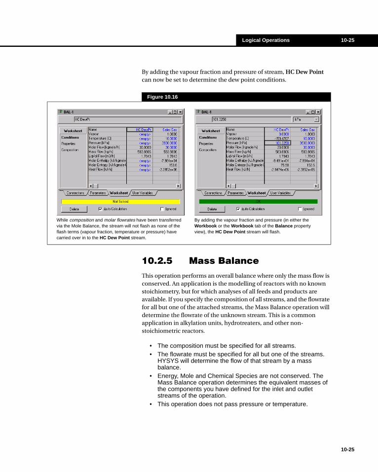
Logical Operations 10-25
By adding the vapour fraction and pressure of stream, HC Dew Point can now be set to determine the dew point conditions.
10.2.5 Mass BalanceThis operation performs an overall balance where only the mass flow is conserved. An application is the modelling of reactors with no known stoichiometry, but for which analyses of all feeds and products are available. If you specify the composition of all streams, and the flowrate for all but one of the attached streams, the Mass Balance operation will determine the flowrate of the unknown stream. This is a common application in alkylation units, hydrotreaters, and other non-stoichiometric reactors.
• The composition must be specified for all streams.• The flowrate must be specified for all but one of the streams.
HYSYS will determine the flow of that stream by a mass balance.
• Energy, Mole and Chemical Species are not conserved. The Mass Balance operation determines the equivalent masses of the components you have defined for the inlet and outlet streams of the operation.
• This operation does not pass pressure or temperature.
Figure 10.16
By adding the vapour fraction and pressure (in either the Workbook or the Workbook tab of the Balance property view), the HC Dew Point stream will flash.
While composition and molar flowrates have been transferred via the Mole Balance, the stream will not flash as none of the flash terms (vapour fraction, temperature or pressure) have carried over in to the HC Dew Point stream.
10-25
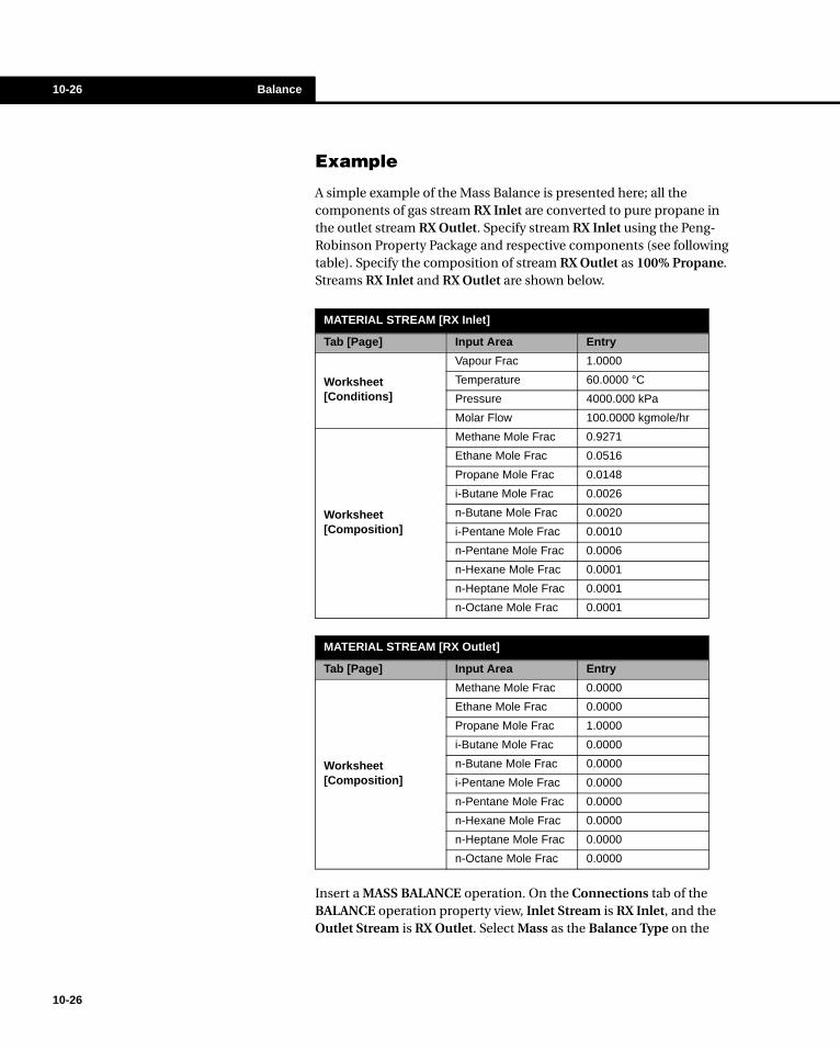
10-26 Balance
10-26
Example
A simple example of the Mass Balance is presented here; all the components of gas stream RX Inlet are converted to pure propane in the outlet stream RX Outlet. Specify stream RX Inlet using the Peng-Robinson Property Package and respective components (see following table). Specify the composition of stream RX Outlet as 100% Propane. Streams RX Inlet and RX Outlet are shown below.
Insert a MASS BALANCE operation. On the Connections tab of the BALANCE operation property view, Inlet Stream is RX Inlet, and the Outlet Stream is RX Outlet. Select Mass as the Balance Type on the
MATERIAL STREAM [RX Inlet]
Tab [Page] Input Area Entry
Worksheet [Conditions]
Vapour Frac 1.0000
Temperature 60.0000 °C
Pressure 4000.000 kPa
Molar Flow 100.0000 kgmole/hr
Worksheet [Composition]
Methane Mole Frac 0.9271
Ethane Mole Frac 0.0516
Propane Mole Frac 0.0148
i-Butane Mole Frac 0.0026
n-Butane Mole Frac 0.0020
i-Pentane Mole Frac 0.0010
n-Pentane Mole Frac 0.0006
n-Hexane Mole Frac 0.0001
n-Heptane Mole Frac 0.0001
n-Octane Mole Frac 0.0001
MATERIAL STREAM [RX Outlet]
Tab [Page] Input Area Entry
Worksheet [Composition]
Methane Mole Frac 0.0000
Ethane Mole Frac 0.0000
Propane Mole Frac 1.0000
i-Butane Mole Frac 0.0000
n-Butane Mole Frac 0.0000
i-Pentane Mole Frac 0.0000
n-Pentane Mole Frac 0.0000
n-Hexane Mole Frac 0.0000
n-Heptane Mole Frac 0.0000
n-Octane Mole Frac 0.0000
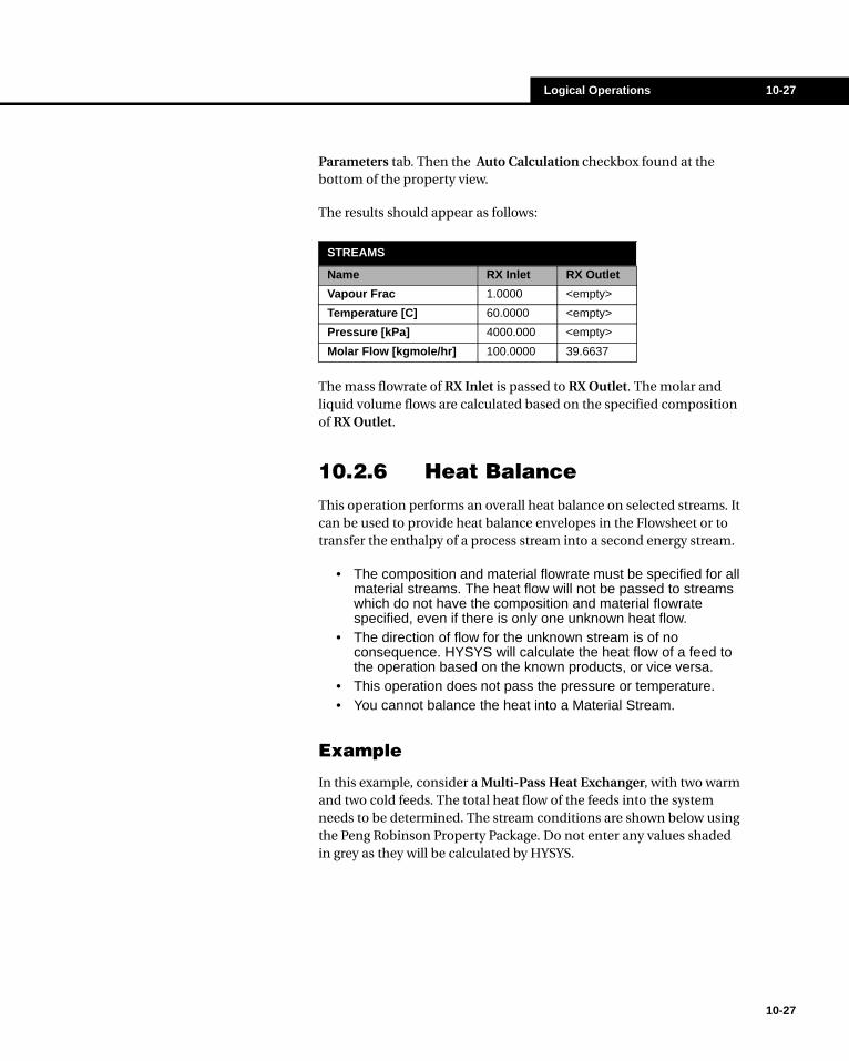
Logical Operations 10-27
Parameters tab. Then the Auto Calculation checkbox found at the bottom of the property view.
The results should appear as follows:
The mass flowrate of RX Inlet is passed to RX Outlet. The molar and liquid volume flows are calculated based on the specified composition of RX Outlet.
10.2.6 Heat BalanceThis operation performs an overall heat balance on selected streams. It can be used to provide heat balance envelopes in the Flowsheet or to transfer the enthalpy of a process stream into a second energy stream.
• The composition and material flowrate must be specified for all material streams. The heat flow will not be passed to streams which do not have the composition and material flowrate specified, even if there is only one unknown heat flow.
• The direction of flow for the unknown stream is of no consequence. HYSYS will calculate the heat flow of a feed to the operation based on the known products, or vice versa.
• This operation does not pass the pressure or temperature.• You cannot balance the heat into a Material Stream.
Example
In this example, consider a Multi-Pass Heat Exchanger, with two warm and two cold feeds. The total heat flow of the feeds into the system needs to be determined. The stream conditions are shown below using the Peng Robinson Property Package. Do not enter any values shaded in grey as they will be calculated by HYSYS.
STREAMS
Name RX Inlet RX Outlet
Vapour Frac 1.0000 <empty>
Temperature [C] 60.0000 <empty>
Pressure [kPa] 4000.000 <empty>
Molar Flow [kgmole/hr] 100.0000 39.6637
10-27

10-28 Balance
10-28
Create an Energy stream and call it QTOTAL. Do not provide any information for this stream.
Set up the Heat Balance as shown in Figure 10.17, where QTOTAL is an energy stream.
Activate the Auto Calculation check box and the calculation should begin. The Heat Flow for energy stream QTOTAL is -3.034e+07 kJ/h.
MATERIAL STREAMS
Name WARM 1 FEED COLD 1 COLD 2
Vapour Frac <empty> <empty> 1 0
Temperature [C] 30.0000 20.0000 <empty> <empty>
Pressure [kPa] 5000.000 5000.000 2000.000 250.0000
Molar Flow [kgmole/hr] 50.0000 100.0000 75.0000 100.0000
Comp Mole Frac [Methane] 0.9500 0.5386 0.9500 0.0200
Comp Mole Frac [Ethane] 0.0500 0.1538 0.0500 0.9800
Comp Mole Frac [Propane] 0.0000 0.0769 0.0000 0.0000
Comp Mole Frac [i-Butane] 0.0000 0.0692 0.0000 0.0000
Comp Mole Frac [n-Butane] 0.0000 0.0615 0.0000 0.0000
Comp Mole Frac [i-Pentane] 0.0000 0.0538 0.0000 0.0000
Comp Mole Frac [n-Pentane] 0.0000 0.0462 0.0000 0.0000
Figure 10.17

Logical Operations 10-29
10.2.7 General BalanceThe General Balance is capable of solving a greater scope of problems. It will solve a set of n unknowns in the n equations developed from the streams attached to the operation. This operation, because of the method of solution, is extremely powerful in the types of problems that it can solve. Not only can it solve unknown flows and compositions in the attached streams (either inlet or outlet can have unknowns), but ratios can be established between components in streams. When the operation determines the solution, the prescribed ratio between components will be maintained.
• The GENERAL BALANCE will solve material and energy balances independently. An Energy Stream is an acceptable inlet or outlet stream.
• The operation will solve unknown flows or compositions, and can have ratios specified between components in one of the streams.
• Ratios can be specified on a mole, mass or liquid volume basis.
Ratios
A Ratio, which is unique to the GENERAL BALANCE, is defined between two components in one of the attached streams. Multiple ratios within a stream (e.g. 1 : 2 : 1 : 1.5) can be set with a single Ratio on a mole, mass or liquid volume basis. Each individual ratio, however (1 : 2, 1 : 1, 1 : 1.5) uses a degree of freedom.
Setting a Ratio
Go to the Parameters tab of the BALANCE operation property view and select the General Balance radio button. The Ratio List group box should now be visible. Click the Add Ratio button to specify component ratios. To view a specific ratio, highlight it and click the View Ratio button. To delete a ratio, you must first view it, and then select the Delete button in that Ratio view.
Figure 10.18
10-29

10-30 Balance
10-30
Ratio View
The following information must be completed on the Ratio definition view:
Number of Unknowns
The GENERAL BALANCE determines the maximum number of equations, and hence unknowns, in the following manner (note that the material and energy balances are solved independently):
• One equation performing an overall molar flow balance.• {Number of Components (nc)} equations performing an
individual molar balance.• {Number of Streams (ns)} equations, each performing a
summation of individual component fractions on a stream by stream basis.
This is the maximum number of equations (1 + nc + ns), and hence unknowns, which can be solved for a system. When ratios are specified, they reduce the available number of unknowns. For each ratio, the number of unknowns used is one less than the number of components in the ratio. For example, for a three-component ratio, two unknowns are used.
Figure 10.19
Required Input Description
Name Enter the name of the Ratio.
Stream Provide the name of the stream.
Ratio Type Specify the Ratio Type: Mole, Mass or Volume.
Component/Ratio
Provide the relative compositions of two or more components. Other components in the stream will be calculated accordingly, and it is not necessary nor advantageous to include these in the table. All ratios must be positive; non-integer values are acceptable.
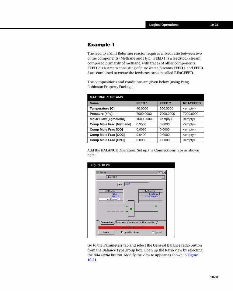
Logical Operations 10-31
Example 1
The feed to a Shift Reformer reactor requires a fixed ratio between two of the components (Methane and H2O). FEED 1 is a feedstock stream composed primarily of methane, with traces of other components. FEED 2 is a stream consisting of pure water. Streams FEED 1 and FEED 2 are combined to create the feedstock stream called REACFEED.
The compositions and conditions are given below (using Peng Robinson Property Package).
Add the BALANCE Operation. Set up the Connections tabs as shown here:
Go to the Parameters tab and select the General Balance radio button from the Balance Type group box. Open up the Ratio view by selecting the Add Ratio button. Modify the view to appear as shown in Figure 10.21.
MATERIAL STREAMS
Name FEED 1 FEED 2 REACFEED
Temperature [C] 40.0000 200.0000 <empty>
Pressure [kPa] 7000.0000 7000.0000 7000.0000
Molar Flow [kgmole/hr] 10000.0000 <empty> <empty>
Comp Mole Frac [Methane] 0.9500 0.0000 <empty>
Comp Mole Frac [CO] 0.0050 0.0000 <empty>
Comp Mole Frac [CO2] 0.0400 0.0000 <empty>
Comp Mole Frac [H2O] 0.0050 1.0000 <empty>
Figure 10.20
10-31
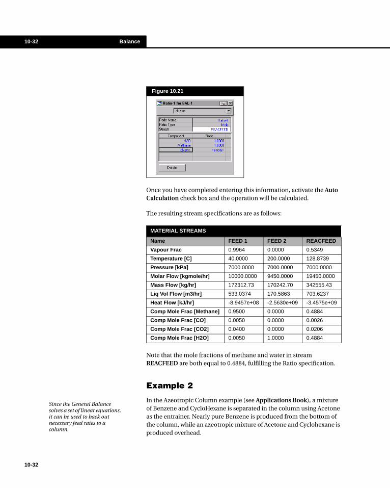
10-32 Balance
10-32
Once you have completed entering this information, activate the Auto Calculation check box and the operation will be calculated.
The resulting stream specifications are as follows:
Note that the mole fractions of methane and water in stream REACFEED are both equal to 0.4884, fulfilling the Ratio specification.
Example 2
In the Azeotropic Column example (see Applications Book), a mixture of Benzene and CycloHexane is separated in the column using Acetone as the entrainer. Nearly pure Benzene is produced from the bottom of the column, while an azeotropic mixture of Acetone and Cyclohexane is produced overhead.
Figure 10.21
MATERIAL STREAMS
Name FEED 1 FEED 2 REACFEED
Vapour Frac 0.9964 0.0000 0.5349
Temperature [C] 40.0000 200.0000 128.8739
Pressure [kPa] 7000.0000 7000.0000 7000.0000
Molar Flow [kgmole/hr] 10000.0000 9450.0000 19450.0000
Mass Flow [kg/hr] 172312.73 170242.70 342555.43
Liq Vol Flow [m3/hr] 533.0374 170.5863 703.6237
Heat Flow [kJ/hr] -8.9457e+08 -2.5630e+09 -3.4575e+09
Comp Mole Frac [Methane] 0.9500 0.0000 0.4884
Comp Mole Frac [CO] 0.0050 0.0000 0.0026
Comp Mole Frac [CO2] 0.0400 0.0000 0.0206
Comp Mole Frac [H2O] 0.0050 1.0000 0.4884
Since the General Balance solves a set of linear equations, it can be used to back out necessary feed rates to a column.

Logical Operations 10-33
The amount of Acetone needed to sufficiently separate the Benzene / CycloHexane azeotrope will be determined. The required Acetone feed rate (based on a fixed feed of Benzene and CycloHexane) involves solving a set of linear equations, which means the General Balance can be used.
The Mass flow rate and compositions of the Azeo feed are specified. The overhead composition from the tower is a near azeotropic mixture of Acetone and CycloHexane, with an Acetone mass fraction of 0.6876. The known stream flows and compositions are (using UNIQUAC):
A General Balance will do individual component balances, while Mole or Mass Balances only perform overall flow balances and cannot solve this problem.
Set up a General Balance with Inlet Streams Azeo Feed and Acetone, and Outlet Streams Azeo Liquid and Benzene. Activate the Auto Calculation check box.
This operation will not completely solve, however the mass flowrates Acetone, Azeo Liquid, and Benzene should now be calculated.
The mass flow of the Acetone stream will immediately be calculated to be 90.18 kg/h.
Note that if you are using the General Balance in this manner, you must delete it prior to running the Column.
MATERIAL STREAMS
Name Azeo Feed Acetone Azeo Liquid Benzene
Mass Flow [kg/hr] 85.0000 <empty> <empty> <empty>
Liq Vol Flow [m3/hr] 0.1023 <empty> <empty> <empty>
Comp Mass Frac [Benzene] 0.5180 0.0000 0.0000 1.0000
Comp Mass Frac [Cyclohexane]
0.4820 0.0000 0.3124 0.0000
Comp Mass Frac [Acetone] 0.0000 1.0000 0.6876 0.0000
STREAMS
Name Azeo Feed Acetone Azeo Liquid Benzene
Mass Flow [kg/hr] 85.00 90.18 131.1 44.03
Comp Mass Frac [Benzene] 0.5180 0.0000 0.0000 1.0000
Comp Mass Frac [Cyclohexane]
0.4820 0.0000 0.3124 0.0000
Comp Mass Frac [Acetone] 0.0000 1.0000 0.6876 0.0000
10-33
10-34 Parametric Unit Operation
10-34
10.3 Parametric Unit Operation
The PARAMETRIC unit operation allows selected unit operations, streams and variables to be solved using a Parametric model. The main function of the Parametric model is to approximates an existing HYSYS model. To build the Parametric model, the Parametric Utility tool is required. This utility integrates Neural Network (NN) technology into its framework. For more information on this utility, refer to Chapter 8 - Utilities of the User’s Guide. A data file with the appropriate data may be used in place of the Parametric Utility.
Using a Parametric model with neural network capability to approximate a HYSYS model will significantly improve the robustness of the model, reduce its calculation time, and improve the overall on-line performance. The accuracy of the model will depend upon the data available and type of model being approximated.
In the flowsheet, the PARAMETRIC unit operation essentially “pulls out” a collection of HYSYS unit operations and replaces them. Therefore, this unit operation may be thought of as a “black box” with inputs and outputs. When the flowsheet is solved, the Parametric model is used in place of the individual HYSYS unit operation models.
To install the PARAMETRIC unit operation, choose Flowsheet - Add Operation from the menu, and select Parametric Unit Operation. To ignore this unit operation, click the Ignore check box at the bottom its the property view.
10.3.1 Design Tab
Connections Page
The Connections page allows the PARAMETRIC unit operation to be connected with the information required for the Parametric model. This information may be found in either a Parametric Utility or a data file.
This tab is always comprised of two groups: Name and Input Data. The rest of the view is unique for the chosen Input Data type.
The Name group lets you define a unique name for the unit operation. The Input Data group allows you to define where the input data to the
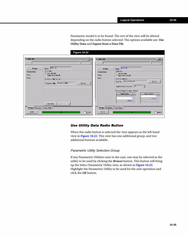
Logical Operations 10-35
Parametric model is to be found. The rest of the view will be altered depending on the radio button selected. The options available are: Use Utility Data and Inputs from a Data File
Use Utility Data Radio Button
When this radio button is selected the view appears as the left hand view in Figure 10.22. This view has one additional group, and two additional buttons available.
Parametric Utility Selection Group
If any Parametric Utilities exist in the case, one may be selected as the utility to be used by clicking the Browse button. This button will bring up the Select Parametric Utility view, as shown in Figure 10.23. Highlight the Parametric Utility to be used for the unit operation and click the OK button.
Figure 10.22
10-35

10-36 Parametric Unit Operation
10-36
Create Utility Button
If a Parametric Utility does not exist in the HYSYS case, or the user wishes to create a new Utility, clicking this button will create one for use in the Parametric unit operation.
View Utility Button
Clicking this button will bring you to the property view for the selected Parametric Utility.
Inputs from a Data File Radio Button
When using this option, the Parametric unit operation does not have to obtain the model parameters from a utility. Instead, an external data file may be used.
Data File Selection Group
Clicking the Browse button allows you to navigate and locate the data file that contains the required information for the Parametric model. The information in the file is comma delimited, and is stored in a *.dat file.
Figure 10.23
The information in the *.dat file is in the format:
input1, input2, input3, .....,ouput1, output2,input1, input2, input3, ....,ouput1, ouput2,

Logical Operations 10-37
Input Units from Data File Group
Using the drop down box, the units used in the data file may be defined.
Modeled Streams for Input and Output
The input and output streams that are being modeled may be selected from the list of existing streams in the drop down box. A new stream may be created and used in the Parametric unit operation by entering a new stream name in the appropriate cell.
Setup Page
The appearance of this page, like the Connections page, is dependant on the radio button selected in the Input Data group on the Connections page. When the Use Utility Data radio button is selected, the view appears as the left hand view in Figure 10.24. When the Inputs from a data file radio button is selected, the view appears as the right hand view in Figure 10.24
Figure 10.24
10-37
10-38 Parametric Unit Operation
10-38
Use Utility Data Radio Button
Available Unit Op Models from Utility
When the Use Utility Data radio button is selected on the Connections page, only one group is available on the Setup page. In this table, all unit operations that have a Parametric model in the selected Parametric Utility are displayed. The name of the unit operation, the status of the model activity, and the operation status of the unit operations are all displayed. The Model Activity may be chosen to be active or inactive by clicking the check box. When the model is inactive, it is only removed from the Parametric Utility.
Inputs from a data file Radio Button
When the Inputs from a Data File radio button is selected on the Connections page, two groups become available on the Setup page: Data Mapping and Training Pair Status.
Data Mapping Group
Two radio buttons are available in this group: Inputs and Outputs. The properties displayed and their descriptions follow.
Training Pair Status Group
Displays the individual training pairs, and indicates whether the pair contains bad data. If an ‘X’ is displayed, there is no bad data. If a check mark is displayed, there is bad data in the data set.
Property Description
Number of Training Pairs
the number of data sets read in from the data file.
Data Point a specific data point within the data file.
Mapped Variable the variable type of the data point. This may be selected from the drop down box.
Variable Type functionality for this column has not been implemented for this version.
Identifier allows the user to enter a unique name to identify the data points.
Low and High Value the minimum and maximum values in the data set.
Bad Variable Status if an ‘X’ is displayed, the data is good. If a check mark is displayed, there is bad data in the data set.
Current Value the value used in the worksheet after training.
A training pair is defined as a set of input data and a pair of output data. In the data file this would be:
input1, input2, input3,....ouput1, output2

Logical Operations 10-39
Notes Page
You can use this page to add any notes pertinent to the unit operation or the simulation case in general.
10.3.2 Parameters TabThe Parameters tab displays the training variables of the attached Parametric Utility. There are four main objects in this view:
Figure 10.25
Figure 10.26
10-39

10-40 Parametric Unit Operation
10-40
Connected Unit Operations
The number of unit operations connected to the Parametric unit operation is displayed in this box.
Manipulated Variables
By selecting the Manipulated radio button, the manipulated variables in the Parametric model will be displayed. The manipulated variables are the variables being modified in the Parametric Utility and obtained from the HYSYS PFD model simulation. The name of the variable is displayed, and the selected status is shown. You may select or deselect the variable for use in the parametric model by clicking the check box. The lower and upper values used for training are also displayed.
Targeted Variables
By selecting the Targeted radio button, the targeted variables in the Parametric model will be displayed. The targeted variable is the same as the Observable variable in the Parametric Utility. Targeted variables are the HYSYS variables whose values are known and used as training data when calculating the Parametric model. The name of the variable is displayed and the selected status is shown. You may select or deselect the variable for use in the Parametric model calculation by clicking the check box. The lower and upper values for training are also displayed.
Train Button
Clicking the Train button will initialize the Parametric Utility training engine to determine the parameters for the Parametric model.
The Parametric model approximates the HYSYS model in the sense that, given the same values of the training input variables, the values of the output variables of the Parametric model must be close to the values from the HYSYS model.
It is important to realize that there are no methods for training neural networks that can “magically” create information that is not contained in the training data. The neural network model is only as good as its training data.

Logical Operations 10-41
10.3.3 Worksheet TabThe Worksheet tab displays the various Conditions, Properties and Compositions of the unit operations, streams, and variables that are using the Parametric model. From here you can use the neural network instead of the flowsheet, and where the training pairs have been used from a file, see how the neural network has modeled the operation from which your training pairs were generated. These objects are displayed as different pages on the tab. For more information on the Workbook, refer to Chapter 4 - Workbook in the User’s Guide.
Figure 10.27
10-41
10-42 Recycle
10-42
10.4 RecycleThe capability of any Flowsheet simulator to solve recycles reliably and efficiently is critical. HYSYS has inherent advantages over other simulators in this respect. It has the unique ability to back-calculate through many operations in a non-sequential manner, allowing many problems with recycle loops to be solved explicitly. For example, most heat recycles can be solved explicitly (without a RECYCLE operation). Material recycles, where downstream material mixes with upstream material, require a RECYCLE operation.
The RECYCLE installs a theoretical block in the process stream. The feed into the block is termed the calculated recycle stream, and the product is the assumed recycle stream. The following steps take place during the convergence process:
1. HYSYS uses the conditions of the assumed stream and solves the Flowsheet up to the calculated stream.
2. HYSYS then compares the values of the calculated stream to those in the assumed stream.
3. Based on the difference between the values, HYSYS modifies the values in the calculated stream and passes the modified values to the assumed stream.
4. The calculation process repeats until the values in the calculated stream match those in the assumed stream within specified tolerances.
To install the RECYCLE operation, choose Add Operation from the Flowsheet menu, and select Recycle. Alternatively, select the Recycle button in the Palette.
Recycle Button
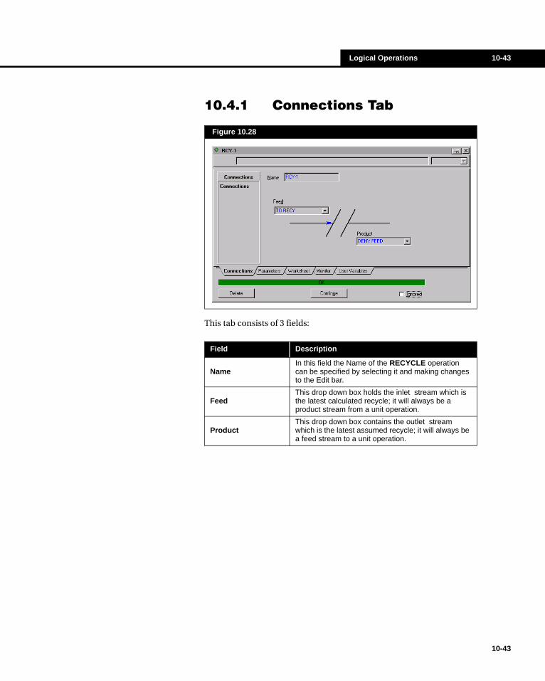
Logical Operations 10-43
10.4.1 Connections Tab
This tab consists of 3 fields:
Figure 10.28
Field Description
NameIn this field the Name of the RECYCLE operation can be specified by selecting it and making changes to the Edit bar.
Feed This drop down box holds the inlet stream which is the latest calculated recycle; it will always be a product stream from a unit operation.
ProductThis drop down box contains the outlet stream which is the latest assumed recycle; it will always be a feed stream to a unit operation.
10-43

10-44 Recycle
10-44
10.4.2 Parameters TabThe Parameters tab contains two pages: Tolerance and Numerical.
Tolerance Page
HYSYS allows you to set the convergence criteria factor for each of the variables listed. The tolerance values you input actually serve as a multiplier for HYSYS’ internal convergence tolerances. The internal absolute tolerances, except flow which is a relative tolerance, are shown below.
For example, the internal tolerance for Temperature is 0.01 and the default multiplier is 10, so the absolute tolerance used by the RECYCLE convergence algorithm is 0.01*10 = 0.1. Therefore, if you are working in SI units, the temperatures of the assumed and calculated recycle
Figure 10.29
HYSYS Internal Tolerances
Variable Internal Tolerance
Vapour Fraction 0.01
Temperature 0.01
Pressure 0.01
Flow 0.001**
Enthalpy 1.00
Composition 0.0001
**Note that flow tolerance is relative rather than absolute
The Internal Vapour Fraction tolerance, when multiplied by the recycle tolerance, is 0.1 which appears to be very loose. However, in most situations, if the other recycle variables have converged, the vapour fraction in the two streams will be identical. The loose Vapour Fraction tolerance is critical for close-boiling mixtures, which can vary widely in vapour fraction with minimal difference in other properties.

Logical Operations 10-45
streams must be within 0.1°C of each other if the RECYCLE is to converge.
A multiplier of 10 (default) is normal and is recommended for most calculations. Values less than 10 are more stringent; that is, the smaller the multiplier, the tighter the convergence tolerance.
It is not required that each of the multipliers be identical. For example, if you are dealing with ppm levels of crucial components, you can set the Composition tolerance multiplier much tighter (smaller) than the others.
Numerical Page
The Numerical page contains the options related to the Wegstein Acceleration Method. This method is used by the RECYCLE to modify the values it passes from the inlet to outlet streams, rather than using direct substitution.
Figure 10.30
To ignore the RECYCLE Operation during calculations, select the Ignore checkbox. HYSYS will completely disregard the operation until you restore it to an active state by clearing the check box.
Numerical Parameters Description
Maximum Iterations The number of iterations before HYSYS stops (default is 10). You may continue with the calculations by selecting the Continue button on the Numerical page.
Wegstein Count The number of iterations before an acceleration step is applied to the next iteration (default is 3).
Flash Type The Flash method to be implemented by the Recycle unit op.
10-45
10-46 Recycle
10-46
Acceleration Options
There are two options for the method of acceleration:
Maximum Number of Iterations
When HYSYS has reached the maximum number of iterations, a warning message will appear stating that the RECYCLE failed to converge in the specified number of iterations. You may then choose whether or not to continue calculations.
If you are starting a new Flowsheet, use a small number of Maximum Iterations, such as 3. Once it is evident that the calculations are proceeding well, the count can be increased. The iterations required will depend not only on the complexity of your Flowsheet, but also on your initial estimate and the convergence tolerances you use.
Damping Factors - Qmax and Qmin
The Wegstein acceleration method uses the results of previous iterations in making its guesses for the recycle stream variables. Assumed values are calculated as follows:
Q maximum/Q minimum
Damping factors for the acceleration step (defaults are 0 and 20).
Acceleration Delay This delays the acceleration until the specified step.
Type Options are Nested or Simultaneous (default is Nested).
Numerical Parameters Description
Acceleration Options
Description
Wegstein Ignores interactions between variables being accelerated.
Dominant Eigenvalue
Includes interactions between variables being accelerated. Further, the Dominant Eigenvalue option is superior when dealing with non-ideal systems or systems with strong interactions between components.
(10.2)Xn 1+ QXn 1 Q–( )Yn+=

Logical Operations 10-47
where: X = Assumed value
Y = Calculated value
n = Iteration number
Q = Acceleration factor
HYSYS determines the actual acceleration (Q) to apply based on the amount of change between successive iterations. The values for Qmax and Qmin set bounds on the amount of acceleration applied. Note from the equation that when Q = 0, direct replacement is used. When Q is negative, acceleration is used. When Q is positive and smaller than 1, damping occurs.
Wegstein Count
The Wegstein Count is the number of RECYCLE iterations before an acceleration step is applied when calculating the next assumed recycle value. The default count is 3; after three iterations (assuming the Acceleration Delay is less than 3), the assumed and calculated recycle values will be compared and the Wegstein acceleration factor will be determined and applied to the next assumed value. When the acceleration factor is not being used (in all iterations up to the Wegstein Count), the next assumed value is determined by direct replacement.
Note that Acceleration Delay takes precedence over the Wegstein Count. This means that for a Acceleration Delay value of x, the initial x iterations will use direct replacement, even if the Wegstein Count is set to less than x. The x+1 iteration will use the acceleration after which the Wegstein Count will apply.
Although acceleration generally works well for most problems, in some cases it may result in over-correction, oscillation and possibly non-convergence. Examples of this type of problem include highly-sensitive
Figure 10.31
If you are finding that your RECYCLE is still oscillating, even with the Wegstein Count set to ensure direct replacement, you can input a slightly larger value for Qmax to damp the direct replacement.
iterations
Recycle Iterations Begin
N W W W W
AD - Acceleration Delay W - Wegstein Count
if W AD then N = AD+1 else if W > AD then N = W
≤
10-47

10-48 Recycle
10-48
recycles and multiple recycle problems with strong interactions among recycles. In cases such as these, direct replacement may be the best method for all iterations. To eliminate the use of acceleration, simply set the Wegstein Count (or Acceleration Delay) to a very high number of iterations (for example, 100) which will never be reached. In the rare instance where even direct replacement causes excessive over-corrections, damping is required. Use the set of parameters discussed below to control this.
Acceleration Delay
The Acceleration Delay parameter delays the acceleration until the specified step. This delay applies to the initial set of iterations and once the specified step is reached the Wegstein Count is applied. That is to say no acceleration is performed until the delay value is reached and after that iteration the acceleration is applied according to the Wegstein count. The default is specified as 2 but now it can be specified to any value.
For example if the ’delay’ is set to 5 and the Wegstein count is 3 then the first 5 iterations will use direct replacement and the sixth will use acceleration then after every third iteration the acceleration step is applied.
Type of Recycle
There are two choices for the type of RECYCLE: Nested and Simultaneous. The Nested option will result in the RECYCLE being called whenever it is encountered during the calculations. In contrast, the Simultaneous option will cause all RECYCLES to be invoked at the same time once all recycle streams have been calculated. If your Flowsheet has a single RECYCLE operation, or if you have multiple recycles which are not connected, use the Nested option (default). If your Flowsheet has multiple inter-connected recycles, use the Simultaneous type.
There are several additional points worth noting about the RECYCLE:
• When the RECYCLE cannot be solved in the number of iterations you specify, HYSYS will stop. If you decide that the problem might converge with more iterations, simply select the Continue button on the Numerical tab. The RECYCLE will initialize the iteration counter and continue until a solution is found or it again runs out of iterations.
The Calculation Level for a RECYCLE (accessed under Main Properties) is 3500, compared to 500 for most streams and operations. This means that the RECYCLE will be solved last among unknown operations. You may set the relative solving order of RECYCLES by modifying the Calculation Level.
Logical Operations 10-49
• If your problem does not converge in a reasonable number of iterations, there are probably constraints in your Flowsheet which make it impossible to solve. In particular, if the size of the recycle stream keeps growing, it is likely that the Flowsheet does not permit all of the material entering the Flowsheet to leave. An example of this occurs in gas plants when you are trying to make a liquid product with a low vapour pressure and a vapour product which must remain free of liquids even at cold temperatures. Often, this leaves no place for intermediate components like propane and butane to go, so they accumulate in the plant recycle streams. It is also possible that the tolerance is too tight for one or more of the RECYCLE variables and cannot be satisfied. This can readily be determined by examining the convergence history and comparing the unconverged variable deviations with their tolerances.
• The logical operations (such as the RECYCLE, ADJUST and CONTROLLER ) are different from other operations in that they actually modify the specifications of a stream. As a result, if you remove any of these operations, the outlet stream specifications remain. Thus, nothing in the Flowsheet is "forgotten" for these operations. You may Delete or Ignore a RECYCLE when you wish to make Flowsheet modifications, but do not want to invoke the iterative routines.
• Tolerance settings are important to a successful RECYCLE solution. This is especially true when multiple recycles are involved. If there is no interaction among the recycles, or if they are inter-connected and are being solved simultaneously, tolerance values can be identical for all RECYCLES if desired. However, if the RECYCLES are nested, tolerances should be made increasingly tighter as you go from the outermost to the innermost RECYCLE. Without this precaution, the outside RECYCLE may not converge.
10.4.3 Worksheet TabThe Worksheet tab displays the various Conditions, Properties and Compositions of the Feed and Product streams. For more information refer to the Workbook.
The Convergence tab provides a history of the Recycle calculations.
10-49

10-50 Recycle
10-50
10.4.4 Monitor Tab
The Setup page allows you to specify which variables you want to view or monitor. To view a variable, select the View check box corresponding to the variable of interest.
The Tables and Plots pages display the convergence information as the calculations are performed in tabular and graphical form respectively. The inlet value, outlet value, and variable are shown, along with the iteration number.
Figure 10.32
Setup page
Tables page Plots page

Logical Operations 10-51
10.4.5 CalculationsHYSYS provides a very simple means of solving recycle problems, and its interactive nature provides a high degree of control and feedback to the user as to how the solution is proceeding. The RECYCLE can be set up as a single unit operation to represent a single recycle stream in a process Flowsheet, or a number of them can be installed to represent multiple recycles, interconnected or nested, as well as a combination of interconnected and nested recycle loops. Similar to the multi-ADJUST operation, the RECYCLE will solve all the recycle loops simultaneously, if requested to do so.
The step-by-step procedure for setting up a recycle is as follows:
1. Make a guess for the assumed recycle stream (temperature, pressure, flow rate, composition).The flow rate can generally be zero, but, obviously, better estimates will result in faster convergence. Note that if the recycle is a feed to a tower, a reasonable estimate is needed to ensure that the column will converge the first time it is run.
2. Build your Flowsheet until the calculated recycle stream can be determined by HYSYS (note that the calculated and assumed recycle streams must have different names).
3. Install the RECYCLE block.
10.4.6 Reducing Convergence Time
Selection of the recycle tear location is vitally important in determining the computer run time to converge the RECYCLE. Although the physical recycle stream itself is often selected as the tear stream, the Flowsheet can be broken at virtually any location. In simulating a complex system, a number of factors must be considered. Following are some general guidelines:
Choose a Tear Location to Minimize the Number of Recycles
Reducing the number of locations where the iterative process is required will save on total convergence time. Choosing the location of the Recycle will depend on the Flowsheet topology. Attempt to choose a point such that specifying the assumed stream will define as many streams downstream as possible. It generally occurs downstream of gathering points and upstream of distribution points. Examples
In Dynamic mode, HYSYS ignores the RECYCLE operation; the outlet stream is identical to the inlet stream.
10-51
10-52 Recycle
10-52
include downstream of mixers (often mixing points where the physical recycle combines with the main stream), and upstream of tees, separators and columns.
Choose a Tear Location to Minimize the Number of Recycle Variables
Variables include vapour fraction, temperature, pressure, flow, enthalpy, and composition. Choose the tear stream so that as many variables as possible are fixed, thus effectively eliminating them as variables and increasing convergence stability. Good choices for these locations are at separator inlets, compressor aftercooler outlets, and trim heater outlets.
Choose a Stable Tear Location
The tear location can be chosen such that fluctuations in the recycle stream have a minimal effect. For example, by placing the tear in a main stream, instead of the physical recycle, the effect of fluctuations will be reduced. The importance of this factor depends on the convergence algorithm. It is more significant when successive substitution is used. Choosing stable tear locations is also important when using simultaneous solution of multi-recycle problems.
10.4.7 Single Recycle ExampleIn this example, a two-phase feed stream (FEED) is mixed with a recycled stream (RECYCLE) and fed to separator V-100. The vapour from V-100 is expanded in expander E-100 and then reflashed in separator V-101. Half of the liquid from this separator is fed to pump P-100 and then recycled back and mixed with the fresh feed.
Avoid choosing tear streams which have variables determined by an ADJUST operation.

Logical Operations 10-53
The conditions and composition of stream FEED are shown here (using the Peng Robinson Property Package).
Figure 10.33
MATERIAL STREAM [Feed]
Tab [Page] Input Area Entry
Worksheet [Conditions]
Temperature 60.0000 °F
Pressure 600.0000 psi
Molar Flow 1 MMSCFH
Worksheet [Composition]
Nitrogen Mole Frac 0.0069
CO2 Mole Frac 0.0138
Methane Mole Frac 0.4827
Ethane Mole Frac 0.1379
Propane Mole Frac 0.0690
i-Butane Mole Frac 0.0621
n-Butane Mole Frac 0.0552
i-Pentane Mole Frac 0.0483
n-Pentane Mole Frac 0.0414
n-Hexane Mole Frac 0.0345
n-Heptane Mole Frac 0.0276
n-Octane Mole Frac 0.0206
10-53

10-54 Recycle
10-54
Add the following unit operations.
SEPARATOR [V-100]
Tab [Page] Input Area Entry
Design [Connections]
Inlets Feed
Vapour Outlet V-100 Vap
Liquid Outlet V-100 Liq
Design [Parameters] Pressure Drop 0 psi
EXPANDER [K-100]
Tab [Page] Input Area Entry
Design [Connections]
Inlet V-100 Vap
Outlet V-101 Feed
Energy V-101 Duty
Worksheet [Conditions]
V-101 Feed Pressure 300 psi
SEPARATOR [V-101]
Tab [Page] Input Area Entry
Design [Connections]
Inlets V-101 Feed
Vapour Outlet V-101Vap
Liquid Outlet V-101 Liq
Design [Parameters] Pressure Drop 1.4500 psi
TEE [TEE-100]
Tab [Page] Input Area Entry
Design [Connections]
Inlet V-101 Liq
Outlets TEE-100 Prod
P-100 Feed
Design [Parameters] Flow Ratio 0.5 (set either one)
PUMP [P-100]
Tab [Page] Input Area Entry
Design [Connections]
Inlet P-100 Feed
Product P-100 Out
Energy P-100 Duty
Design [Parameters] Efficiency 75%
Worksheet [Conditions]
P-100 Out Pressure 600 psi
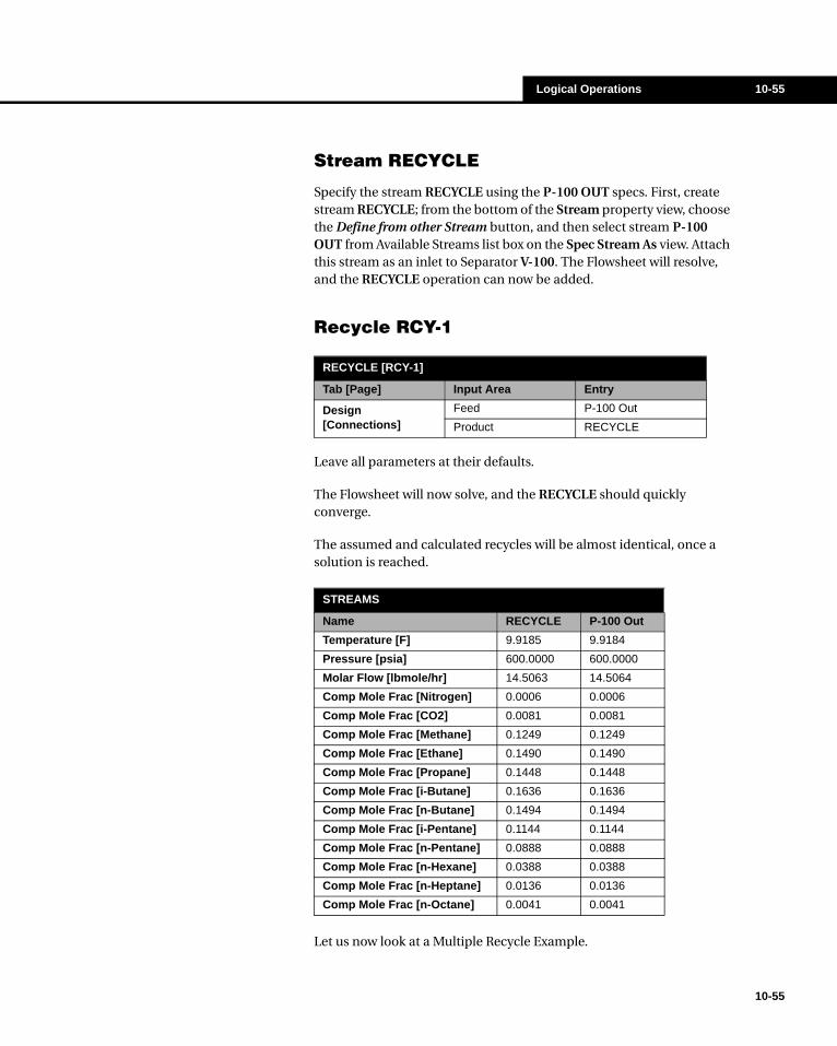
Logical Operations 10-55
Stream RECYCLE
Specify the stream RECYCLE using the P-100 OUT specs. First, create stream RECYCLE; from the bottom of the Stream property view, choose the Define from other Stream button, and then select stream P-100 OUT from Available Streams list box on the Spec Stream As view. Attach this stream as an inlet to Separator V-100. The Flowsheet will resolve, and the RECYCLE operation can now be added.
Recycle RCY-1
Leave all parameters at their defaults.
The Flowsheet will now solve, and the RECYCLE should quickly converge.
The assumed and calculated recycles will be almost identical, once a solution is reached.
Let us now look at a Multiple Recycle Example.
RECYCLE [RCY-1]
Tab [Page] Input Area Entry
Design [Connections]
Feed P-100 Out
Product RECYCLE
STREAMS
Name RECYCLE P-100 Out
Temperature [F] 9.9185 9.9184
Pressure [psia] 600.0000 600.0000
Molar Flow [lbmole/hr] 14.5063 14.5064
Comp Mole Frac [Nitrogen] 0.0006 0.0006
Comp Mole Frac [CO2] 0.0081 0.0081
Comp Mole Frac [Methane] 0.1249 0.1249
Comp Mole Frac [Ethane] 0.1490 0.1490
Comp Mole Frac [Propane] 0.1448 0.1448
Comp Mole Frac [i-Butane] 0.1636 0.1636
Comp Mole Frac [n-Butane] 0.1494 0.1494
Comp Mole Frac [i-Pentane] 0.1144 0.1144
Comp Mole Frac [n-Pentane] 0.0888 0.0888
Comp Mole Frac [n-Hexane] 0.0388 0.0388
Comp Mole Frac [n-Heptane] 0.0136 0.0136
Comp Mole Frac [n-Octane] 0.0041 0.0041
10-55
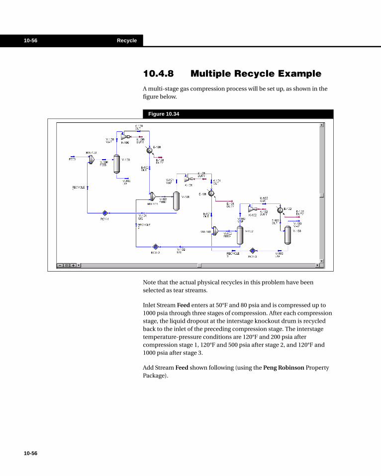
10-56 Recycle
10-56
10.4.8 Multiple Recycle ExampleA multi-stage gas compression process will be set up, as shown in the figure below.
Note that the actual physical recycles in this problem have been selected as tear streams.
Inlet Stream Feed enters at 50°F and 80 psia and is compressed up to 1000 psia through three stages of compression. After each compression stage, the liquid dropout at the interstage knockout drum is recycled back to the inlet of the preceding compression stage. The interstage temperature-pressure conditions are 120°F and 200 psia after compression stage 1, 120°F and 500 psia after stage 2, and 120°F and 1000 psia after stage 3.
Add Stream Feed shown following (using the Peng Robinson Property Package).
Figure 10.34

Logical Operations 10-57
To set up this Flowsheet, a series of separators, compressors, coolers and mixers have to be installed as shown in the figure. The recycle streams will be added after the operations have been installed. Install the operations as described on the next few pages.
Leave all parameters at their defaults unless otherwise indicated.
MATERIAL STREAM [Feed]
Tab [Page] Input Area Entry
Worksheet [Conditions]
Temperature 50.0000 °F
Pressure 80.0000 psi
Molar Flow 2500.0000 lbmole/hr
Worksheet [Composition]
Nitrogen Mole Frac 0.0069
CO2 Mole Frac 0.0138
Methane Mole Frac 0.4827
Ethane Mole Frac 0.1379
Propane Mole Frac 0.0690
i-Butane Mole Frac 0.0621
n-Butane Mole Frac 0.0552
i-Pentane Mole Frac 0.0483
n-Pentane Mole Frac 0.0414
n-Hexane Mole Frac 0.0345
n-Heptane Mole Frac 0.0276
n-Octane Mole Frac 0.0206
MIXER [MIX-100]
Tab [Page] Input Area Entry
Design [Connections]
Inlet Feed
Outlet V-100 Feed
Design [Parameters] Pressure Assignment Set Outlet to Lowest Inlet
10-57

10-58 Recycle
10-58
The Recycled Stream Recycle 1 will be added to this mixer after all the operations have been installed.
Specify the temperature and pressure of stream E-100 Out as 120 °F and 200 psi.
The Recycled Stream Recycle 2 to this mixer will be added after all the operations have been installed.
SEPARATOR [V-100]
Tab [Page] Input Area Entry
Design [Connections]
Inlets V-100 Feed
Vapour Outlet V-100 Vao
Liquid Outlet V-100 Liq
COMPRESSOR [K-100]
Tab [Page] Input Area Entry
Design [Connections]
Inlet V-100 Vap
Outlet K-100 Out
Energy K-100 Duty
COOLER [E-100]
Tab [Page] Input Area Entry
Design [Connections]
Feed Stream K-100 Out
Product Stream E-100 Out
Energy Stream E-100 Duty
Design [Parameters] Pressure Drop 5 psia
MIXER [MIX-101]
Tab [Page] Input Area Entry
Design [Connections]
InletE-100 Out
Outlet V-101 Feed
Design [Parameters] Pressure Assignment Set Unknown Outlet to Lowest Inlet
SEPARATOR [V-101]
Tab [Page] Input Area Entry
Design [Connections]
Feed V-101 Feed
Vapour Outlet V-101 Vap
Liquid Outlet V-101 Liq
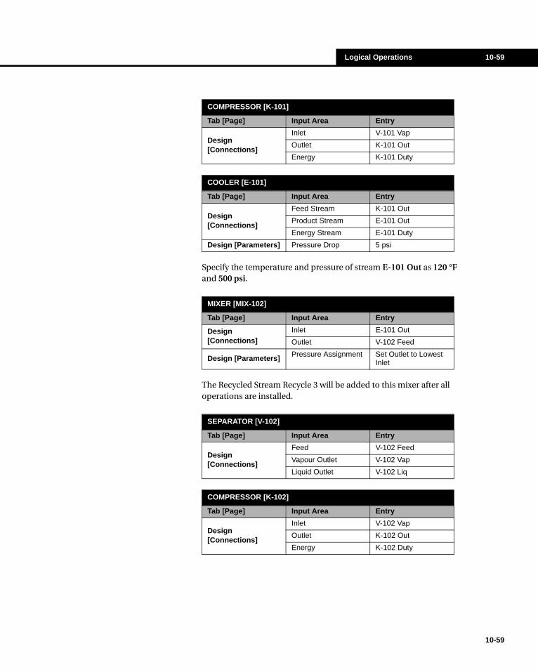
Logical Operations 10-59
Specify the temperature and pressure of stream E-101 Out as 120 °F and 500 psi.
The Recycled Stream Recycle 3 will be added to this mixer after all operations are installed.
COMPRESSOR [K-101]
Tab [Page] Input Area Entry
Design [Connections]
Inlet V-101 Vap
Outlet K-101 Out
Energy K-101 Duty
COOLER [E-101]
Tab [Page] Input Area Entry
Design [Connections]
Feed Stream K-101 Out
Product Stream E-101 Out
Energy Stream E-101 Duty
Design [Parameters] Pressure Drop 5 psi
MIXER [MIX-102]
Tab [Page] Input Area Entry
Design [Connections]
Inlet E-101 Out
Outlet V-102 Feed
Design [Parameters] Pressure Assignment Set Outlet to Lowest Inlet
SEPARATOR [V-102]
Tab [Page] Input Area Entry
Design [Connections]
Feed V-102 Feed
Vapour Outlet V-102 Vap
Liquid Outlet V-102 Liq
COMPRESSOR [K-102]
Tab [Page] Input Area Entry
Design [Connections]
Inlet V-102 Vap
Outlet K-102 Out
Energy K-102 Duty
10-59

10-60 Recycle
10-60
Specify the temperature and pressure of stream E-102 Out as 120 °F and 1000 psi.
Next, add the recycled streams, by selecting the Define from other Stream button from the bottom of the Material stream property view and using the Spec Stream As view to define them using another stream’s properties.
Recycle Streams• Specify Stream Recycle 1 as Stream V-101 Liq and connect
as a feed to MIX-100• Specify Stream Recycle 2 as Stream V-102 Liq and connect
as a feed to MIX-101• Specify Stream Recycle 3 as Stream V-103 Liq and connect
as a feed to MIX-102
The properties of Streams V-101 Liq, V-102 Liq and V-103 Liq serve as the initial estimates for the recycle streams. Before adding the RECYCLE operations, you may want to put the Flowsheet into hold mode.
RECYCLE Operations• RCY-1 - Feed: Stream V-101 Liq; Product: Stream Recycle 1• RCY-2 - Feed: Stream V-102 Liq; Product: Stream Recycle 2• RCY-3 - Feed: Stream V-103 Liq; Product: Stream Recycle 3
Solve the Flowsheet, and you will obtain the following converged material stream conditions as shown in Figure 10.35.
COOLER [E-102]
Tab [Page] Input Area Entry
Design [Connections]
Feed Stream K-102 Out
Product Stream E-102 Out
Energy Stream E-102 Duty
Design [Parameters] Pressure Drop 5 psi
SEPARATOR [V-103]
Tab [Page] Input Area Entry
Design [Connections]
Feed E-102 Out
Vapour Outlet V-103 Vap
Liquid Outlet V-103 Liq
By using this sequence, better starting points for the Recycle streams will be used.
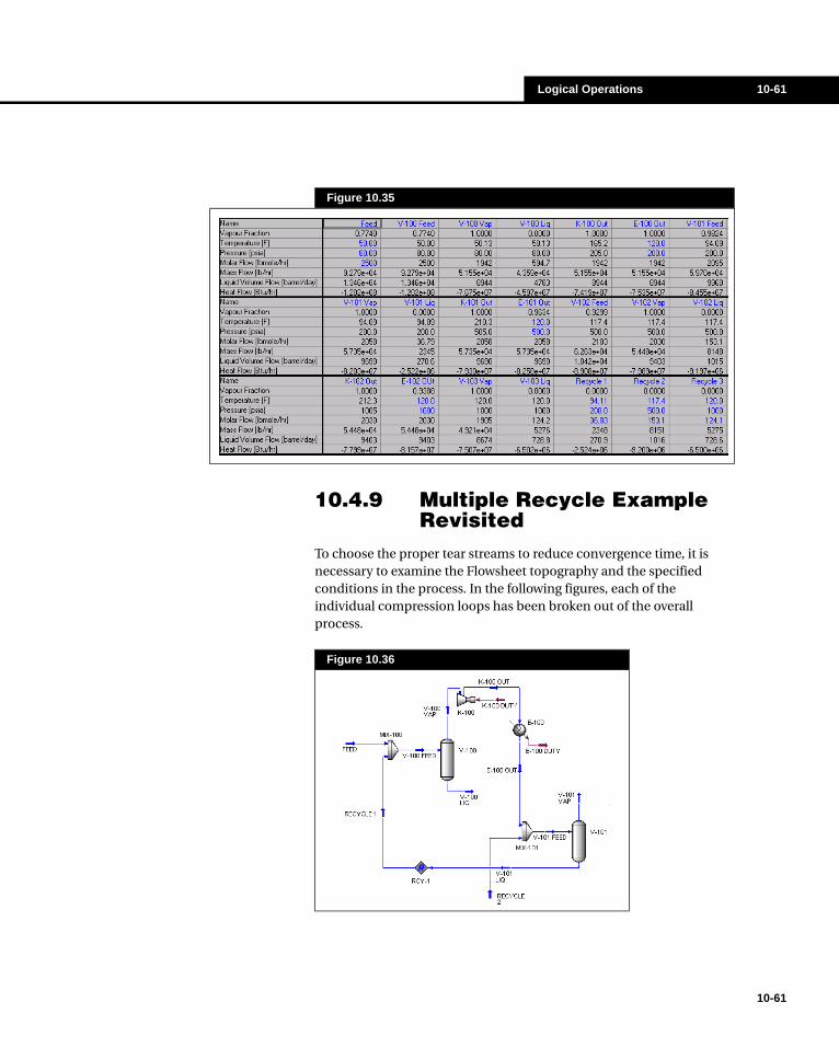
Logical Operations 10-61
10.4.9 Multiple Recycle Example Revisited
To choose the proper tear streams to reduce convergence time, it is necessary to examine the Flowsheet topography and the specified conditions in the process. In the following figures, each of the individual compression loops has been broken out of the overall process.
Figure 10.35
Figure 10.36
10-61
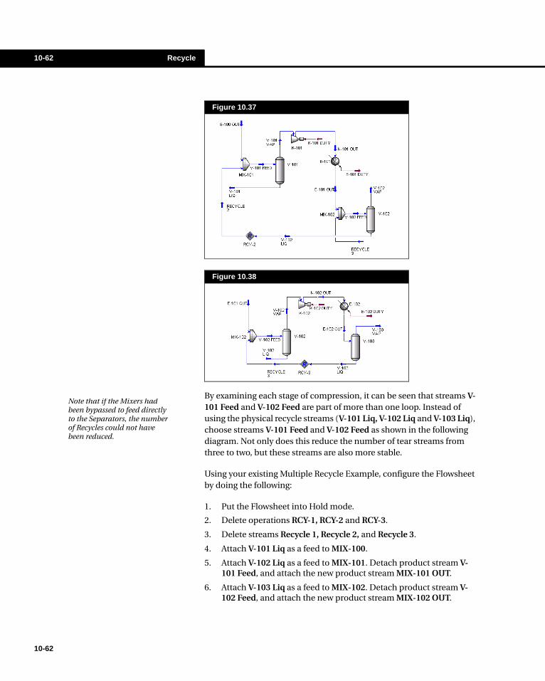
10-62 Recycle
10-62
By examining each stage of compression, it can be seen that streams V-101 Feed and V-102 Feed are part of more than one loop. Instead of using the physical recycle streams (V-101 Liq, V-102 Liq and V-103 Liq), choose streams V-101 Feed and V-102 Feed as shown in the following diagram. Not only does this reduce the number of tear streams from three to two, but these streams are also more stable.
Using your existing Multiple Recycle Example, configure the Flowsheet by doing the following:
1. Put the Flowsheet into Hold mode.
2. Delete operations RCY-1, RCY-2 and RCY-3.
3. Delete streams Recycle 1, Recycle 2, and Recycle 3.
4. Attach V-101 Liq as a feed to MIX-100.
5. Attach V-102 Liq as a feed to MIX-101. Detach product stream V-101 Feed, and attach the new product stream MIX-101 OUT.
6. Attach V-103 Liq as a feed to MIX-102. Detach product stream V-102 Feed, and attach the new product stream MIX-102 OUT.
Figure 10.37
Figure 10.38
Note that if the Mixers had been bypassed to feed directly to the Separators, the number of Recycles could not have been reduced.
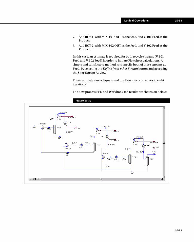
Logical Operations 10-63
7. Add RCY-1, with MIX-101 OUT as the feed, and V-101 Feed as the Product.
8. Add RCY-2, with MIX-102 OUT as the feed, and V-102 Feed as the Product.
In this case, an estimate is required for both recycle streams (V-101 Feed and V-102 Feed) in order to initiate Flowsheet calculations. A simple and satisfactory method is to specify both of these streams as Feed, by selecting the Define from other Stream button and accessing the Spec Stream As view.
These estimates are adequate and the Flowsheet converges in eight iterations.
The new process PFD and Workbook tab results are shown on below:
Figure 10.39
10-63
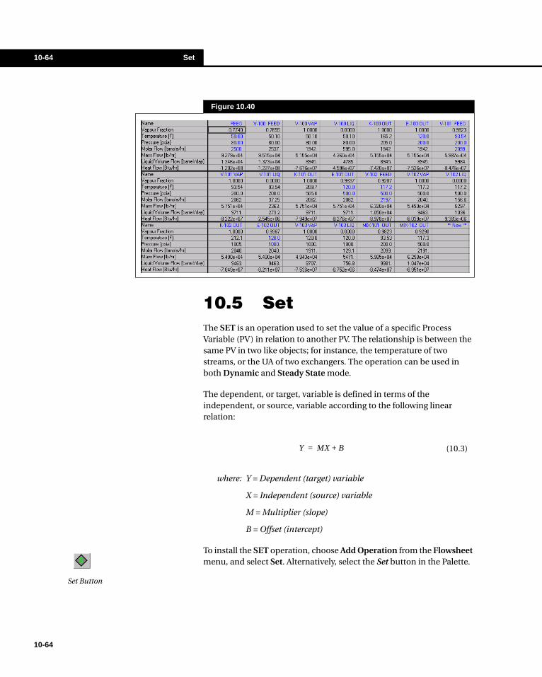
10-64 Set
10-64
10.5 SetThe SET is an operation used to set the value of a specific Process Variable (PV) in relation to another PV. The relationship is between the same PV in two like objects; for instance, the temperature of two streams, or the UA of two exchangers. The operation can be used in both Dynamic and Steady State mode.
The dependent, or target, variable is defined in terms of the independent, or source, variable according to the following linear relation:
where: Y = Dependent (target) variable
X = Independent (source) variable
M = Multiplier (slope)
B = Offset (intercept)
To install the SET operation, choose Add Operation from the Flowsheet menu, and select Set. Alternatively, select the Set button in the Palette.
Figure 10.40
(10.3)Y MX B+=
Set Button
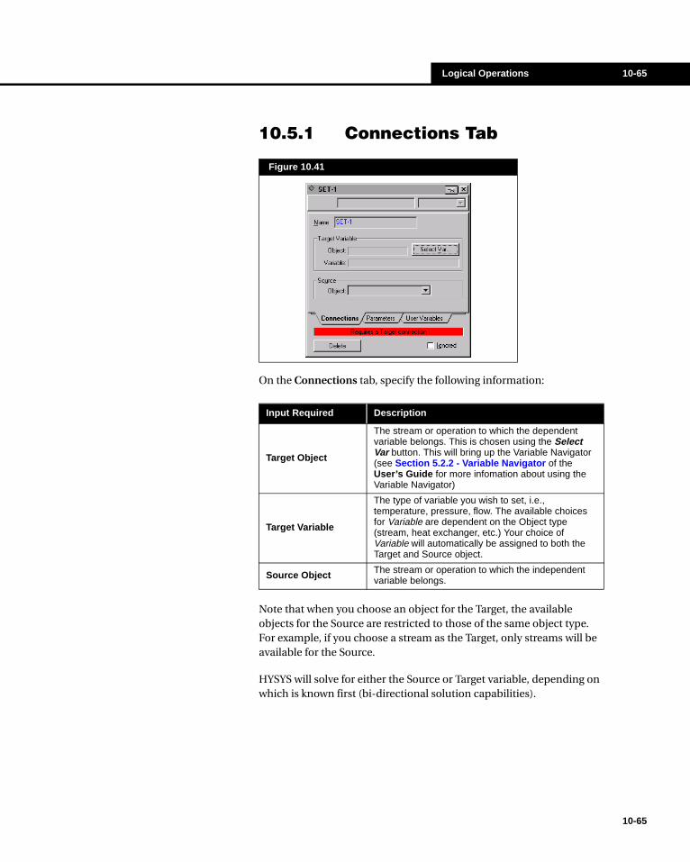
Logical Operations 10-65
10.5.1 Connections Tab
On the Connections tab, specify the following information:
Note that when you choose an object for the Target, the available objects for the Source are restricted to those of the same object type. For example, if you choose a stream as the Target, only streams will be available for the Source.
HYSYS will solve for either the Source or Target variable, depending on which is known first (bi-directional solution capabilities).
Figure 10.41
Input Required Description
Target Object
The stream or operation to which the dependent variable belongs. This is chosen using the Select Var button. This will bring up the Variable Navigator (see Section 5.2.2 - Variable Navigator of the User’s Guide for more infomation about using the Variable Navigator)
Target Variable
The type of variable you wish to set, i.e., temperature, pressure, flow. The available choices for Variable are dependent on the Object type (stream, heat exchanger, etc.) Your choice of Variable will automatically be assigned to both the Target and Source object.
Source Object The stream or operation to which the independent variable belongs.
10-65
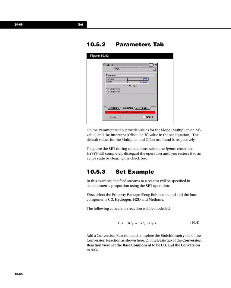
10-66 Set
10-66
10.5.2 Parameters Tab
On the Parameters tab, provide values for the Slope (Multiplier, or ’M’-value) and the Intercept (Offset, or ’B’-value in the set equation). The default values for the Multiplier and Offset are 1 and 0, respectively.
To ignore the SET during calculations, select the Ignore checkbox. HYSYS will completely disregard the operation until you restore it to an active state by clearing the check box.
10.5.3 Set ExampleIn this example, the feed streams to a reactor will be specified in stoichiometric proportion using the SET operation.
First, select the Property Package (Peng Robinson), and add the four components CO, Hydrogen, H2O and Methane.
The following conversion reaction will be modelled:
Add a Conversion Reaction and complete the Stoichiometry tab of the Conversion Reaction as shown here. On the Basis tab of the Conversion Reaction view, set the Base Component to be CO, and the Conversion to 80%.
Figure 10.42
(10.4)CO 3H2+ CH4 H2O+→

Logical Operations 10-67
If you wish, create a Reaction Set, and add the Conversion Reaction to that Set. This is not necessary, however, as the reaction is automatically added to the Global Rxn Set. Add the Global Rxn Set to the fluid package by clicking on the Add to FP button. Once this is done, exit the Basis Environment.
There will be two feed streams to the reactor (Separator), one being pure CO, and the other pure H2. The feed streams are displayed below. The Molar Flowrate of CO Feed is known and equal to 100 kgmole/hr.
Figure 10.43
STREAMS
Name CO Feed H2 Feed
Vapour Frac 1.0000 1.0000
Temperature [C] 550.0000 550.0000
Pressure [kPa] 1000.0000 1000.0000
Molar Flow [kgmole/hr] 100.0000 <empty>
Comp Mole Frac [CO] 1.0000 0.0000
Comp Mole Frac [H2] 0.0000 1.0000
Comp Mole Frac [H2O] 0.0000 0.0000
Comp Mole Frac [Methane] 0.0000 0.0000
10-67
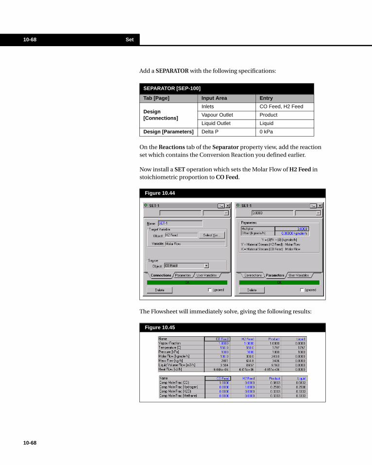
10-68 Set
10-68
Add a SEPARATOR with the following specifications:
On the Reactions tab of the Separator property view, add the reaction set which contains the Conversion Reaction you defined earlier.
Now install a SET operation which sets the Molar Flow of H2 Feed in stoichiometric proportion to CO Feed.
The Flowsheet will immediately solve, giving the following results:
SEPARATOR [SEP-100]
Tab [Page] Input Area Entry
Design [Connections]
Inlets CO Feed, H2 Feed
Vapour Outlet Product
Liquid Outlet Liquid
Design [Parameters] Delta P 0 kPa
Figure 10.44
Figure 10.45

Logical Operations 10-69
Although this example is trivial, this type of application can be useful when applied to larger problems. For instance, in Flowsheets where feed(s) to the reactor are recycled, the SET can ensure that their relative flowrates are always in stoichiometric proportion.
10.6 Spreadsheet
The SPREADSHEET applies the functionality of Spreadsheet programs to Flowsheet modelling. With essentially complete access to all process variables, the SPREADSHEET is extremely powerful and has many applications in HYSYS.
The SPREADSHEET can be used to manipulate or perform custom calculations on Flowsheet variables. Because it is an operation, calculations will be performed automatically; Spreadsheet cells are updated when Flowsheet variables change.
One application of the SPREADSHEET is the calculation of pressure drop during dynamic operation of a Heat Exchanger. In the HYSYS Heat Exchanger, the pressure drop remains constant on both sides regardless of flow. However, using the Spreadsheet, the actual pressure drop on one or both sides of the exchanger could be calculated as a function of flow.
Complex mathematical formulas can be created, using syntax which is similar to conventional Spreadsheets. Arithmetic, logarithmic and
Figure 10.46
In situations where non-pure streams are being fed to a reactor, particularly when a RECYCLE is involved, the General Balance is the preferred route.
The HYSYS SPREADSHEET has standard row/column functionality. You can import a variable, or enter a number or formula anywhere in the spreadsheet.
10-69

10-70 Spreadsheet
10-70
trigonometric functions are examples of the mathematical functionality available in the Spreadsheet. The Spreadsheet also provides logical programming in addition to its comprehensive mathematical capabilities. Boolean logic is supported, which allows you to compare the value of two or more variables using logical operators, and then perform the appropriate action depending on that result.
You may import virtually any variable in the simulation into the Spreadsheet, and you can export a cell’s value to any specifiable field in your simulation. There are two ways of importing and exporting variables to and from the Spreadsheet:
When you are using the Spreadsheet to return a result back to the Flowsheet, you must consider its application in terms of the overall calculation sequence, particularly when Recycles are involved. If the Spreadsheet performs a calculation and sends the results back upstream, the potential exists for creating inconsistencies as the full effect of the previous Recycle loop has not propagated through the Flowsheet. By using the Calculation Sequencing option (see Section 7.3.1 - Main Properties of the User’s Guide), you can minimize the potential for problems of this nature.
To install the SPREADSHEET, choose Add Operation from the Flowsheet menu, and select Spreadsheet. Alternatively, you could select the Spreadsheet button in the Palette.
Note that when using the Dragging Variables method, the views have to be non-modal.
Method Import/Export
Description
Using the Variable Navigator
On the Connections tab, select the Add Import or Add Export button. Then using the Variable Navigator, select the variable you wish to import or export.
Dragging Variables
Using the secondary mouse button, simply click the variable value you wish to import, and drag it to the desired location in the Spreadsheet. If you are exporting the variable, drag it from the Spreadsheet to an appropriate location.
Spreadsheet Button

Logical Operations 10-71
10.6.1 Spreadsheet FunctionsThe HYSYS Spreadsheet has extensive mathematical and logical function capability. To view the available Spreadsheet Functions and Expressions, select the Function Help button. Note that this Help Window has three tabs, Mathematical Expressions, Logical Expressions and Mathematical Functions.
General Math Functions
The following arithmetic functions are supported:
All functions must be preceded by "+" (straight math) or "@" (special functions - logarithmic, trigonometric, logical, etc.)
Examples are "+A4/B5" and "@ABS(A4-B5)".
General Operations Method of Application View
Addition
Use the "+" symbol.
Subtraction
Use the "-" symbol.
Multiplication
Use the "*" symbol.
Division
Use the "/" symbol, typically located on the numeric keypad, or next to the right SHIFT key. (Do not use the "\" symbol).
Absolute Value
"@Abs".
10-71

10-72 Spreadsheet
10-72
Several other mathematical functions are also available:
Calculation Hierarchy
The usual hierarchy of calculation is used (Brackets, Exponents, Division and Multiplication, Addition and Subtraction). For example:
+6+4/2 = 8 (not 5)
since division is performed before addition. However,
+(6+4)/2 = 5
because any expressions in parentheses are calculated first.
Logarithmic Functions
Advanced Operations
Method of Application View
Power
Use the "^" symbol.
Example: +3^3 = 27
Example 2: +27^(1/3)=3. Note that the parentheses are required in this case, since the cube root of 27 (or 27 to the power of one-third) is desired. See Calculation Hierarchy (following page).
Square Root
"@SQRT".
Example: @sqrt(16) = 4. Note that capitalization is irrelevant. You may also use "@RT" to calculate a square root (Example: @rt(16)=4)
Pi
Simply enter "+pi" to represent the number 3.1415...
Factorial
Use the "!" symbol. Example: +5!-120=0
Log Function Method of Application View
Natural Log
"@ln".
Example: @ln(2.73)=1.004
Base 10 Log
"@log".
Example: @log(1000)=3
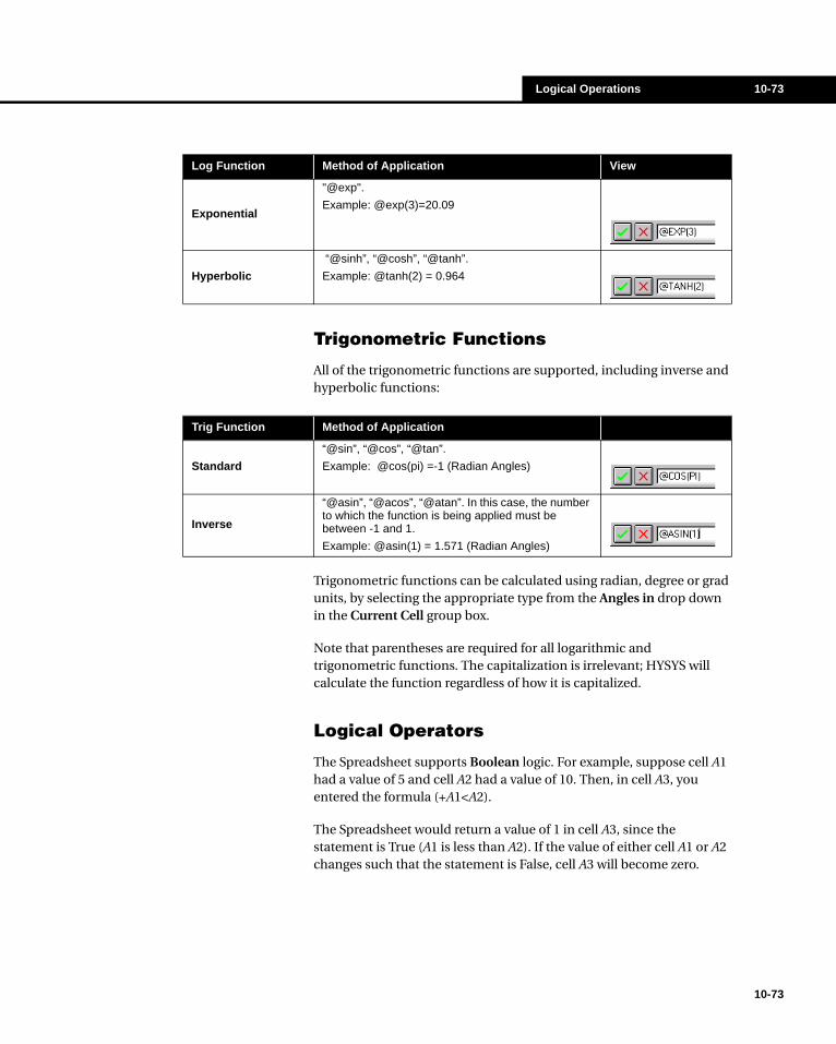
Logical Operations 10-73
Trigonometric Functions
All of the trigonometric functions are supported, including inverse and hyperbolic functions:
Trigonometric functions can be calculated using radian, degree or grad units, by selecting the appropriate type from the Angles in drop down in the Current Cell group box.
Note that parentheses are required for all logarithmic and trigonometric functions. The capitalization is irrelevant; HYSYS will calculate the function regardless of how it is capitalized.
Logical Operators
The Spreadsheet supports Boolean logic. For example, suppose cell A1 had a value of 5 and cell A2 had a value of 10. Then, in cell A3, you entered the formula (+A1<A2).
The Spreadsheet would return a value of 1 in cell A3, since the statement is True (A1 is less than A2). If the value of either cell A1 or A2 changes such that the statement is False, cell A3 will become zero.
Exponential
"@exp".
Example: @exp(3)=20.09
Hyperbolic
“@sinh”, “@cosh”, “@tanh”.
Example: @tanh(2) = 0.964
Log Function Method of Application View
Trig Function Method of Application
Standard
“@sin”, “@cos”, “@tan”.
Example: @cos(pi) =-1 (Radian Angles)
Inverse
“@asin”, “@acos”, “@atan”. In this case, the number to which the function is being applied must be between -1 and 1.
Example: @asin(1) = 1.571 (Radian Angles)
10-73

10-74 Spreadsheet
10-74
You may use the following operators:
IF/THEN/ELSE Statements
The general format of IF/THEN/ELSE statements is:
“@if (condition) then (if true) else (if false)”
The condition is a logical expression, such as "B1 == 15".
For example, suppose cell A3 contained the number 6. The statement
“@if (A3>10) then (10) else (A3/2)”
would result in the value 3 being displayed in the cell.
Boolean Method of Application
Equal To "=="
Not Equal To "!="
Greater Than ">"
Less Than "<"
Greater Than or Equal to ">="
Less Than or Equal to "<="
Figure 10.47

Logical Operations 10-75
10.6.2 Spreadsheet Interface
Importing and Exporting Variables by dragging
You may drag the contents of any cell in the simulation into the Spreadsheet. Simply position the pointer on that field, click and hold the secondary mouse button, and drag the value to any cell in the Spreadsheet. Note that the window from which you are dragging must be unpinned (non-modal). The Spreadsheet window is modal by default.
When you drag to a cell in the Spreadsheet, you will see the "bulls-eye" cursor. Release the secondary mouse button, and the value will be dropped in that cell. In the Imported From field in the Current Cell group box (which appears when the cursor is on an imported cell), you will see the Object for that particular cell. The Object Variable is displayed in the Variable field. Every time you make a change to (or HYSYS re-calculates) a variable you have placed in the Spreadsheet, your data will be updated appropriately.
You always need to provide an ELSE clause (IF/THEN statements are not accepted).
Parentheses are mandatory for IF/THEN/ELSE statements.
A non-Modal view has a Minimizing and Maximizing buttons in the upper-right had corner, and has a double border. You can drag variables outside a non-Modal view.
A Modal view has a ‘pin’ in the upper-right hand corner, and has a single border. You cannot drag variables outside a Modal view.
Select the pin to convert a Modal property view to a Non-Modal view.
10-75
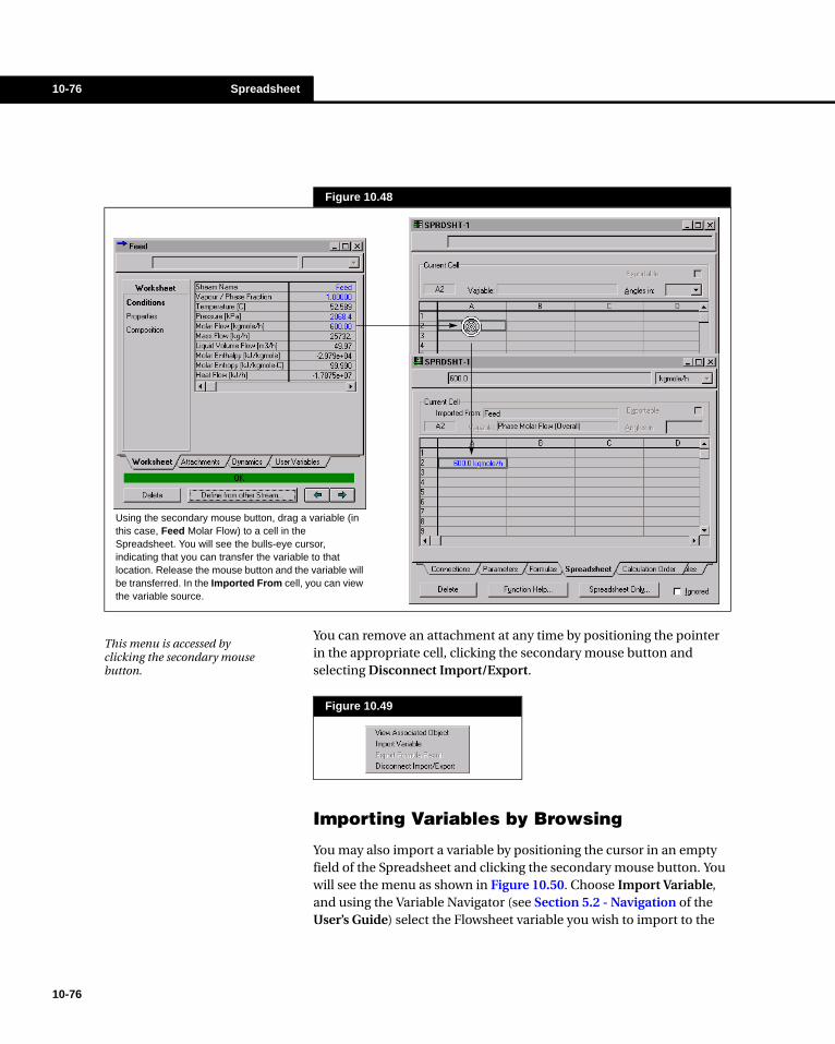
10-76 Spreadsheet
10-76
You can remove an attachment at any time by positioning the pointer in the appropriate cell, clicking the secondary mouse button and selecting Disconnect Import/Export.
Importing Variables by Browsing
You may also import a variable by positioning the cursor in an empty field of the Spreadsheet and clicking the secondary mouse button. You will see the menu as shown in Figure 10.50. Choose Import Variable, and using the Variable Navigator (see Section 5.2 - Navigation of the User’s Guide) select the Flowsheet variable you wish to import to the
Figure 10.48
Using the secondary mouse button, drag a variable (in this case, Feed Molar Flow) to a cell in the Spreadsheet. You will see the bulls-eye cursor, indicating that you can transfer the variable to that location. Release the mouse button and the variable will be transferred. In the Imported From cell, you can view the variable source.
Figure 10.49
This menu is accessed by clicking the secondary mouse button.
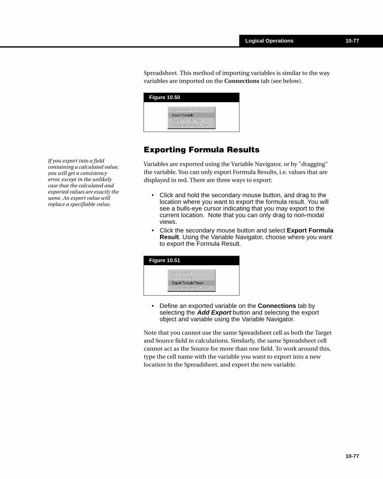
Logical Operations 10-77
Spreadsheet. This method of importing variables is similar to the way variables are imported on the Connections tab (see below).
Exporting Formula Results
Variables are exported using the Variable Navigator, or by "dragging" the variable. You can only export Formula Results, i.e. values that are displayed in red. There are three ways to export:
• Click and hold the secondary mouse button, and drag to the location where you want to export the formula result. You will see a bulls-eye cursor indicating that you may export to the current location. Note that you can only drag to non-modal views.
• Click the secondary mouse button and select Export Formula Result. Using the Variable Navigator, choose where you want to export the Formula Result.
• Define an exported variable on the Connections tab by selecting the Add Export button and selecting the export object and variable using the Variable Navigator.
Note that you cannot use the same Spreadsheet cell as both the Target and Source field in calculations. Similarly, the same Spreadsheet cell cannot act as the Source for more than one field. To work around this, type the cell name with the variable you want to export into a new location in the Spreadsheet, and export the new variable.
Figure 10.50
Figure 10.51
If you export into a field containing a calculated value, you will get a consistency error, except in the unlikely case that the calculated and exported values are exactly the same. An export value will replace a specifiable value.
10-77

10-78 Spreadsheet
10-78
Note that when you export a variable from a Spreadsheet cell, that variable is given the same units as the units of the location to which you exported it.
For example, suppose you wanted to assign the pressure of stream Feed to another stream. In cell B1, enter the formula +A1, and then export the contents of the cell to the pressure cell of the appropriate stream, using one of the methods outlined above.
View Associated Object
You can view an object associated with a specific cell by clicking the secondary mouse button, and selecting View Associated Object. For instance, if you dragged the temperature of a stream from the WorkSheet into the Spreadsheet, the Associated Object would be that stream. When you select View Associated Object, you will be taken to the property view for that Stream. Note that you can also view the associated object of an imported cell, by double-clicking on that cell.
If there is no object associated with the current cell, this menu selection will be disabled.
Figure 10.52
Figure 10.53
Because the contents of Cell A1 cannot be both an import and export, the formula +A1 is entered in Cell B1. Cell B1 is then exported to the RECYCLE 1 pressure.
For this simple example, you could use the SET Operation. For more complex situations, you must use the Spreadsheet.

Logical Operations 10-79
10.6.3 Spreadsheet Tabs
Connections Tab
On the Connections tab, you can add, edit and delete Imports and Exports. As mentioned earlier, you may also import and export variables by dragging to and from the Spreadsheet.
To add an import, select the Add Import button, and choose the variable using the Variable Navigator (For more information, see Section 5.2 - Navigation of the User’s Guide). In the Cell column, type or select from the drop down list the Spreadsheet cell to be connected to that variable. When you move to the Spreadsheet tab, that variable will appear in the cell you specified.
You may edit or delete an import by positioning the cursor in the appropriate row, and selecting the Edit Import or Delete Import buttons. Adding, editing and deleting Exports is performed in a similar manner.
Note that you may also edit the Spreadsheet Name on this tab.
Figure 10.54
10-79

10-80 Spreadsheet
10-80
Parameters Tab
On this tab of the Spreadsheet property view, you can set the dimensions of the Spreadsheet and choose a Unit Set.
Exportable Cells
Prior to explaining how the Exportable cells are created, the difference between exporting from the Spreadsheet (assigning a value from the Spreadsheet to a Process Variable) or importing from the Spreadsheet (accessing a Spreadsheet variable from another object) must be explained. Results that are exported from the Spreadsheet to a specifiable process variable can only be connected once, i.e., the same cell cannot be connected to two process variables.
Figure 10.55
Spreadsheet Parameters
Description
Number of Columns and Rows
You may set the dimensions of the Spreadsheet. Note that if you set the dimensions of the Spreadsheet smaller than what is already specified, you will permanently delete the contents of cells which are removed. For instance, the contents of cell A4 will be deleted when you set the Number of Rows to 3.
Units
You may choose a Unit Set for the Spreadsheet. All values in the Spreadsheet will be displayed using units from the set you have chosen (see Section 7.7.5 - Preferences)
The Visible Name and Variable Name columns display variables which can be exported. The fact that a variable appears in this list does not necessarily mean that the variable has been exported.

Logical Operations 10-81
However, locations in the program which can import from the Spreadsheet (e.g. PID CONTROLLER Cascade Source, ADJUST Target Variable or DataBook Variable) can access any cell, including those which are being exported to a Flowsheet process variable. The Exportable Cells list has been created to allow objects which use the Variable Navigator to access variables associated with the Spreadsheet.
The Exportable Cells group box will display all cells which can be exported (including those which have been exported). The Visible Name, Variable Name and Variable Type will either display the information you have specified for the associated cell on the Spreadsheet itself, or will contain the information appropriate to the process variable that the cell has been exported to. In the former case, this information is modifiable; you can change it here or on the Spreadsheet itself. In the latter, you cannot modify the information as it is set by the process variable the cell has been exported to. For instance, if you export a Spreadsheet value to the Separator Valve Opening cell, the Variable Name and Variable Type will be Valve Opening and Percent, respectively.
You can edit the Variable Name and Variable Type for all non-exported variables which appear in the list (Note that Spreadsheet variables attached to the Controller, Adjusts and Databook are not exported, but are imported from that Object).
When you access the Spreadsheet as the Object (e.g. - through the Variable Navigator), the contents of the Visible Name cell will appear in the Variable List.
Figure 10.56
There are four variables in the Variable List for SPRDSHT-1 corresponding to cells B1, B4, and B7 and D1. Note that the Variable Names were added manually.
When you use the Variable Navigator and select SPRDSHT-1 as the Object you will see cells B1, B2, B3, B4, B5, B7 and D1 in the Variable List.
10-81

10-82 Spreadsheet
10-82
Formulas Tab
The Formulas tab displays a summary of all the formulas included in your spreadsheet. The table lists the name of the cell the formula is located in, the formula and the result of the formula.
Spreadsheet Tab
The Spreadsheet tab, with the labelled rows and columns, is similar to conventional Spreadsheets.
From this tab, you can import and export variables, disconnect imports/exports, view associated object views, define formula expressions, and modify variable names.
Figure 10.57
Spreadsheet Function
For More Information
Importing and Exporting
See Subsections: Importing and Exporting Variables by dragging, and Importing Variables by Browsing.
Associated Object Views
See Subsection: View Associated Object.
Formula Expressions
See Subsection: Spreadsheet Functions.
Variable Names See Subsection: Exportable Cells.
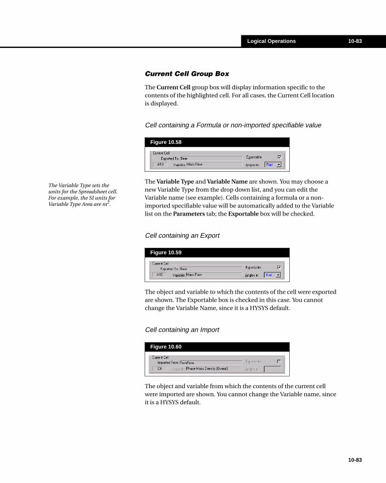
Logical Operations 10-83
Current Cell Group Box
The Current Cell group box will display information specific to the contents of the highlighted cell. For all cases, the Current Cell location is displayed.
Cell containing a Formula or non-imported specifiable value
The Variable Type and Variable Name are shown. You may choose a new Variable Type from the drop down list, and you can edit the Variable name (see example). Cells containing a formula or a non-imported specifiable value will be automatically added to the Variable list on the Parameters tab; the Exportable box will be checked.
Cell containing an Export
The object and variable to which the contents of the cell were exported are shown. The Exportable box is checked in this case. You cannot change the Variable Name, since it is a HYSYS default.
Cell containing an Import
The object and variable from which the contents of the current cell were imported are shown. You cannot change the Variable name, since it is a HYSYS default.
Figure 10.58
Figure 10.59
Figure 10.60
The Variable Type sets the units for the Spreadsheet cell. For example, the SI units for Variable Type Area are m2.
10-83

10-84 Spreadsheet
10-84
Calculation Order Tab
The Calculation Order tab allows you to set the calculation level of each of the cells in the spreadsheet. Click the Calculation Order Help button to see the rules for setting the calculation levels.
User Variables Tab
The User Variables tab allows you to create and implement variables in the HYSYS simulation case. For more information on implementing User Variables, see Chapter 5 - User Variables in the Customization Guide.
Function Help and Spreadsheet Only buttons
Selecting the Function Help button allows you to view the available Spreadsheet Functions and Expressions. Note that this Help Window has three tabs, Mathematical Expressions, Logical Expressions and Mathematical Functions. See Section 10.6.1 - Spreadsheet Functions for more information.
Select the Spreadsheet Only button to view just the Spreadsheet cells in a separate window. This feature is useful when you have completely set up the Spreadsheet and you only want to view the cell results.
Figure 10.61

Logical Operations 10-85
10.6.4 Spreadsheet ExampleIn this example, the Spreadsheet will be used to calculate the Reynold’s Number for a water stream flowing through a pipe.
Specify the stream as shown here, using the Peng Robinson property package.
The Reynold’s Number is calculated as follows:
where: d = Characteristic length (diameter)
u = Fluid velocity
ρ = Fluid density
µ = Fluid viscosity
Add a SPREADSHEET and move to the Spreadsheet tab. The steps involved in setting up the Spreadsheet shown are described below:
Diameter
The diameter of the pipe is assumed to be 2 cm. In cell B1, enter the number 0.02. Initially, this number will not have any units. Although it is not necessary for this example, you can add length units by positioning the cursor in cell B1, and selecting Length from the Variable Type drop down. HYSYS then gives that number the default length units which is dependent on the Unit Set defined on the Parameters tab. In this case, the default length unit is metres.
MATERIAL STREAM [Feed]
Tab [Page] Input Area Entry
Worksheet [Conditions]
Temperature 30.0000 °C
Pressure 101.3250 kPa
Mass Flow 400.0000 kg/hr
Worksheet [Composition]
H2O Mole Frac 1.0000
(10.5)Reduρ
µ----------=
All of the text in columns A and C was entered by typing it in the appropriate cells. You may wish to enter this text as you do the example, to improve the clarity of your Spreadsheet.
10-85
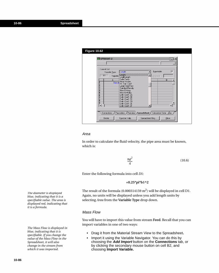
10-86 Spreadsheet
10-86
Area
In order to calculate the fluid velocity, the pipe area must be known, which is:
Enter the following formula into cell D1:
+0.25*pi*b1^2
The result of the formula (0.000314159 m2) will be displayed in cell D1. Again, no units will be displayed unless you add length units by selecting Area from the Variable Type drop down.
Mass Flow
You will have to import this value from stream Feed. Recall that you can import variables in one of two ways:
• Drag it from the Material Stream View to the Spreadsheet.• Import it using the Variable Navigator. You can do this by
choosing the Add Import button on the Connections tab, or by clicking the secondary mouse button on cell B2, and choosing Import Variable.
Figure 10.62
(10.6)πd2
4---------
The diameter is displayed blue, indicating that it is a specifiable value. The area is displayed red, indicating that it is a formula.
The Mass Flow is displayed in blue, indicating that it is specifiable. If you change the value of the Mass Flow in the Spreadsheet, it will also change in the stream from which it was imported.

Logical Operations 10-87
When you have successfully imported the Mass Flow, it will be displayed in the cell. As well, in the Current Cell group box, HYSYS will show that the variable is Mass Flow, and was imported from stream Feed.
Density
Import the Mass Density into cell B3 the same way you imported the Mass Flow. The density is dependent on the basic stream properties (temperature and pressure) and is therefore not specifiable. It is displayed black, indicating that it is a calculated value and cannot be changed.
Velocity
The velocity can now be calculated as follows:
where: = Mass flowrate
ρ = Density
A = Area
Enter this formula into cell B4:
+(B2/3600)/(B3*D1)
It is necessary to divide the mass flow by 3600 to convert the time unit from hours to seconds.
Viscosity
Import the Viscosity of stream Feed into cell B5. The Viscosity is a calculated value and cannot be specified.
Reynold’s Number
The Reynold’s Number can now be calculated by entering the following formula into cell B7:
+(B1*B4*B3)/(B5/1000)
(10.7)u m· ρA( )⁄=
m·
10-87
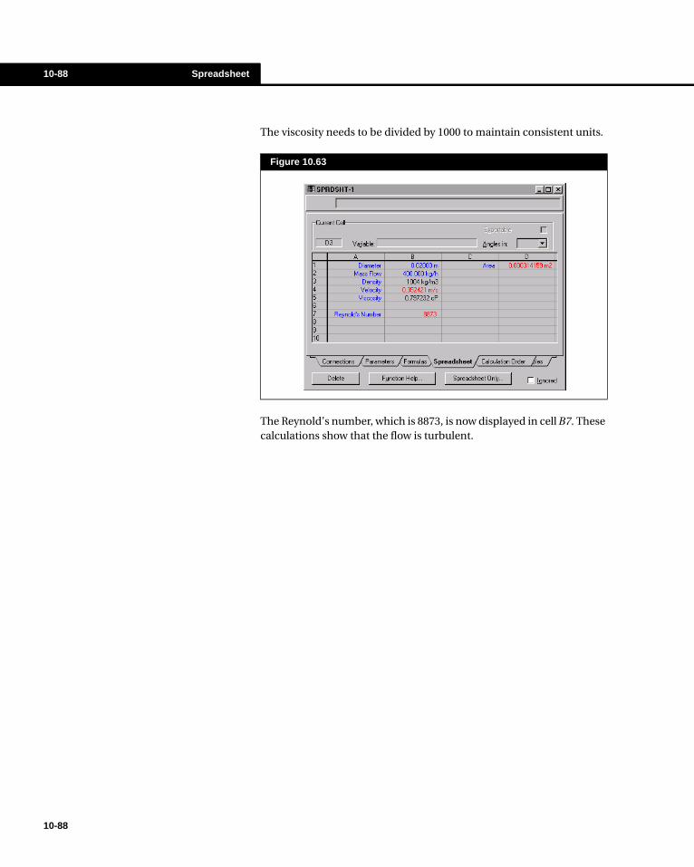
10-88 Spreadsheet
10-88
The viscosity needs to be divided by 1000 to maintain consistent units.
The Reynold’s number, which is 8873, is now displayed in cell B7. These calculations show that the flow is turbulent.
Figure 10.63

Optimizer 11-1
11 Optimizer
11-1
11.1 Optimizer ..................................................................................................... 3
11.2 Optimizer View............................................................................................ 4
11.2.1 Variables Tab.......................................................................................... 411.2.2 Functions Tab ......................................................................................... 511.2.3 Parameters Tab ...................................................................................... 611.2.4 Monitor Tab............................................................................................. 8
11.3 Optimization Schemes............................................................................... 9
11.3.1 Function Setup ....................................................................................... 911.3.2 BOX Method......................................................................................... 1011.3.3 SQP Method..........................................................................................1111.3.4 Mixed Method........................................................................................1111.3.5 Fletcher Reeves Method .......................................................................1111.3.6 Quasi-Newton Method.......................................................................... 12
11.4 Optimizer Tips........................................................................................... 12
11.5 Optimizer Examples ................................................................................. 13
11.5.1 Part I: Solving Multiple UA Exchangers................................................ 1311.5.2 Part II: Optimizing Overall UA .............................................................. 19
11.6 References ................................................................................................ 22

11-2
11-2
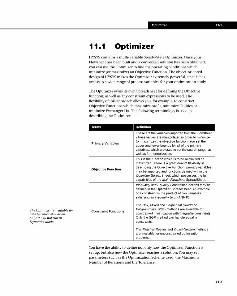
Optimizer 11-3
11.1 OptimizerHYSYS contains a multi-variable Steady-State Optimizer. Once your Flowsheet has been built and a converged solution has been obtained, you can use the Optimizer to find the operating conditions which minimize (or maximize) an Objective Function. The object-oriented design of HYSYS makes the Optimizer extremely powerful, since it has access to a wide range of process variables for your optimization study.
The Optimizer owns its own Spreadsheet for defining the Objective function, as well as any constraint expressions to be used. The flexibility of this approach allows you, for example, to construct Objective Functions which maximize profit, minimize Utilities or minimize Exchanger UA. The following terminology is used in describing the Optimizer.
You have the ability to define not only how the Optimizer Function is set up, but also how the Optimizer reaches a solution. You may set parameters such as the Optimization Scheme used, the Maximum Number of Iterations and the Tolerance.
Terms Definition
Primary Variables
These are the variables imported from the Flowsheetwhose values are manipulated in order to minimize (or maximize) the objective function. You set the upper and lower bounds for all of the primary variables, which are used to set the search range, aswell as for normalization.
Objective Function
This is the function which is to be minimized or maximized. There is a great deal of flexibility in describing the Objective Function; primary variablesmay be imported and functions defined within the Optimizer SpreadSheet, which possesses the full capabilities of the Main Flowsheet SpreadSheet.
Constraint Functions
Inequality and Equality Constraint functions may be defined in the Optimizer SpreadSheet. An example of a constraint is the product of two variables satisfying an inequality (e.g. -A*B<K).
The Box, Mixed and Sequential Quadratic Programming (SQP) methods are available for constrained minimization with inequality constraints.Only the SQP method can handle equality constraints.
The Fletcher-Reeves and Quasi-Newton methods are available for unconstrained optimization problems.
The Optimizer is available for Steady-State calculations only; it will not run in Dynamics mode.
11-3
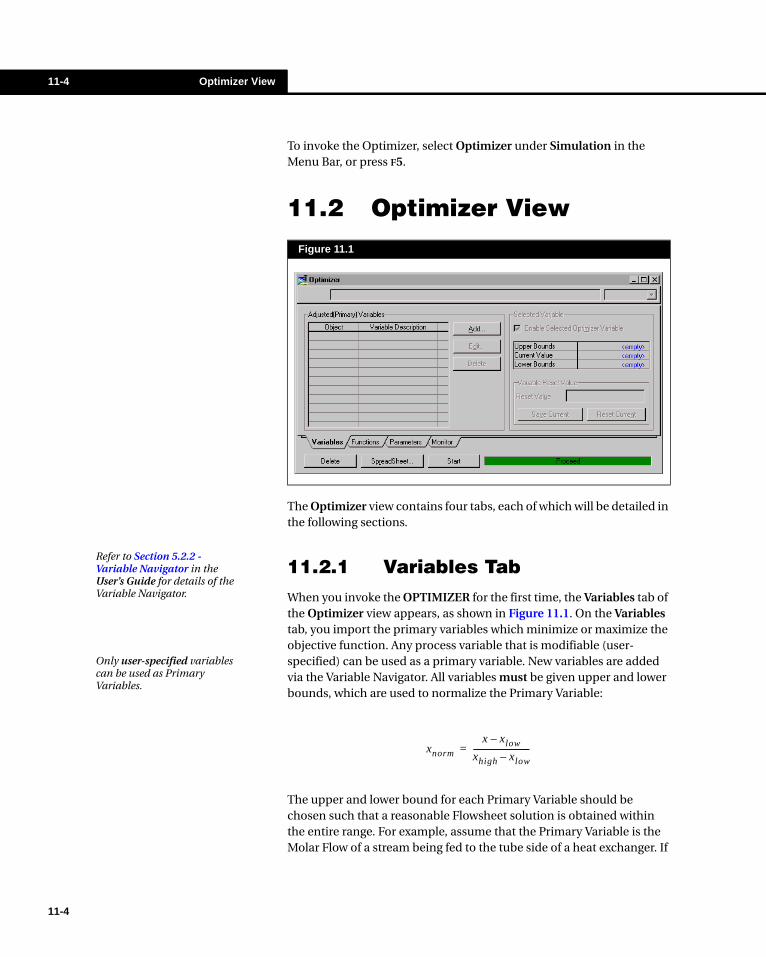
11-4 Optimizer View
11-4
To invoke the Optimizer, select Optimizer under Simulation in the Menu Bar, or press F5.
11.2 Optimizer View
The Optimizer view contains four tabs, each of which will be detailed in the following sections.
11.2.1 Variables TabWhen you invoke the OPTIMIZER for the first time, the Variables tab of the Optimizer view appears, as shown in Figure 11.1. On the Variables tab, you import the primary variables which minimize or maximize the objective function. Any process variable that is modifiable (user-specified) can be used as a primary variable. New variables are added via the Variable Navigator. All variables must be given upper and lower bounds, which are used to normalize the Primary Variable:
The upper and lower bound for each Primary Variable should be chosen such that a reasonable Flowsheet solution is obtained within the entire range. For example, assume that the Primary Variable is the Molar Flow of a stream being fed to the tube side of a heat exchanger. If
Figure 11.1
Refer to Section 5.2.2 - Variable Navigator in the User’s Guide for details of the Variable Navigator.
Only user-specified variables can be used as Primary Variables.
xnorm
x xlow–
xhigh xlow–----------------------------=
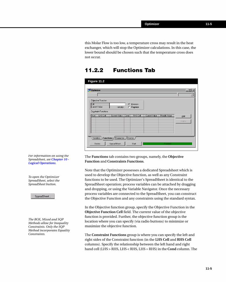
Optimizer 11-5
this Molar Flow is too low, a temperature cross may result in the heat exchanger, which will stop the Optimizer calculations. In this case, the lower bound should be chosen such that the temperature cross does not occur.
11.2.2 Functions Tab
The Functions tab contains two groups, namely, the Objective Function and Constraints Functions.
Note that the Optimizer possesses a dedicated Spreadsheet which is used to develop the Objective function, as well as any Constraint functions to be used. The Optimizer’s SpreadSheet is identical to the SpreadSheet operation; process variables can be attached by dragging and dropping, or using the Variable Navigator. Once the necessary process variables are connected to the SpreadSheet, you can construct the Objective Function and any constraints using the standard syntax.
In the Objective function group, specify the Objective Function in the Objective Function Cell field. The current value of the objective function is provided. Further, the objective function group is the location where you can specify (via radio buttons) to minimize or maximize the objective function.
The Constraint Functions group is where you can specify the left and right sides of the Constraint function (in the LHS Cell and RHS Cell columns). Specify the relationship between the left hand and right hand cell (LHS > RHS, LHS < RHS, LHS = RHS) in the Cond column. The
Figure 11.2
For information on using the Spreadsheet, see Chapter 10 - Logical Operations.
To open the Optimizer SpreadSheet, select the SpreadSheet button.
The BOX, Mixed and SQP Methods allow for Inequality Constraints. Only the SQP Method incorporates Equality Constraints.
11-5
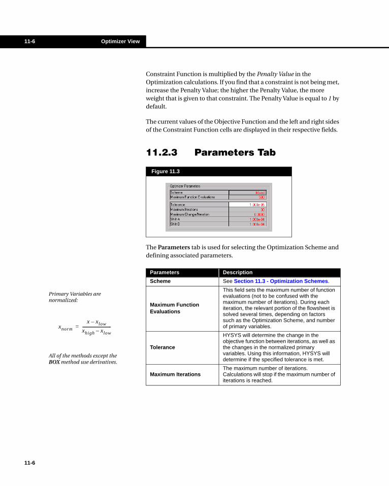
11-6 Optimizer View
11-6
Constraint Function is multiplied by the Penalty Value in the Optimization calculations. If you find that a constraint is not being met, increase the Penalty Value; the higher the Penalty Value, the more weight that is given to that constraint. The Penalty Value is equal to 1 by default.
The current values of the Objective Function and the left and right sides of the Constraint Function cells are displayed in their respective fields.
11.2.3 Parameters Tab
The Parameters tab is used for selecting the Optimization Scheme and defining associated parameters.
Figure 11.3
Parameters Description
Scheme See Section 11.3 - Optimization Schemes.
Maximum Function Evaluations
This field sets the maximum number of function evaluations (not to be confused with the maximum number of iterations). During each iteration, the relevant portion of the flowsheet is solved several times, depending on factors such as the Optimization Scheme, and number of primary variables.
Tolerance
HYSYS will determine the change in the objective function between iterations, as well as the changes in the normalized primary variables. Using this information, HYSYS will determine if the specified tolerance is met.
Maximum IterationsThe maximum number of iterations. Calculations will stop if the maximum number of iterations is reached.
Primary Variables are normalized:
xnorm
x xlow–
xhigh xlow–----------------------------=
All of the methods except the BOX method use derivatives.

Optimizer 11-7
Maximum Change / Iteration
The maximum allowable change in the normalized primary variables between iterations. For instance, assume the maximum change per iteration is 0.3 (this is the default value). If you have specified molar flow as a primary variable with range 0 to 200 kgmole/hr, then the maximum change in one iteration would be (200)(0.3) or 60 kgmole/hr.
Shift A / Shift B
Derivatives of the objective function and/or constraint functions with respect to the primary variables are generally required and are calculated using numerical differentiation.
The numerical derivative is calculated from the following relationship:
where: x = Perturbed variable (normalized)
xshift = Shift interval (normalized)
Derivatives are calculated using:
where: y2 = The value of the affected variable corresponding to x+xshift
y1 = The value of the affected variable corresponding to x
Prior to each step, the Optimizer needs to determine the gradient of the optimization surface at the current location. The Optimizer moves each primary variable by a value of xShift (which due to the size of Shift A and Shift B will be a very small step). The derivative is then evaluated for every function (Objective and Constraint) using the values for y at the two locations of x. From this information and the Optimizer history, the next step direction and size are chosen.
Parameters Description
Shift B ensures that the Shift interval xShift will never be zero.
In general, it should not be necessary to change Shift A and Shift B from their defaults.
Some Schemes move all Primary variables simultaneously, while others move them sequentially.
To determine each derivative, a variable evaluation must be made in addition to the Main Flowsheet evaluation which is done after each iteration (main step change). Therefore, if there are two primary variables, there will be three function evaluations for every iteration.
Note that if you have selected the Mixed Optimizer Scheme, the Box and SQP methods are used in sequence - this is the reason why the Function Evaluations are reset part way through the calculations.
xshift ShiftA∗x ShiftB+=
∂y∂x-----
y2 y1–
xshift----------------=
11-7

11-8 Optimizer View
11-8
11.2.4 Monitor Tab
The Monitor tab displays the values of the Objective Function, primary variables and constraint functions during the Optimizer calculations. New information is updated only when there is an improvement in the value of the Objective Function. The constraint values are positive if inequality constraints are satisfied and negative if inequality constraints are not satisfied.
There are three buttons that can be seen in the Optimizer view, no matter which page is being viewed. These include:
Figure 11.4
Buttons Description
Delete Erases all the current information from the Optimizer and its Spreadsheet.
Spreadsheet Accesses the Optimizer’s dedicated Spreadsheet.
Start/StopStarts or stops the Optimizer calculations. An objective function must be defined prior to the start of the calculations.
Optimizer 11-9
11.3 Optimization Schemes
11.3.1 Function SetupThe Optimizer manipulates the values of a set of primary variables in order to minimize (or maximize) a user-defined Objective Function, constructed from any number of process variables.
where: x1,x2,...,xn are process variables.
Each primary variable, x0, will be manipulated within a specified range:
The general equality and inequality constraints are:
The constraint functions should generally not use the primary variables.
All primary variables are normalized from the lower bound through the upper bound. Thus, reasonable lower and upper bounds must be supplied. Exceedingly high or low variable bounds should obviously be avoided as they may result in numerical problems when scaling. An initial starting point must be supplied, and it should be within the feasible region. Constraints are optional and are not supported by all of the Optimization Schemes.
If HYSYS fails to evaluate the objective function or any of the constraint functions, the Optimizer will reduce the incremental step of the last
In general, the primary variables should not be part of the Objective Function.
(11.1)min f x1 x2 x3 ... xn, , , ,( )
xi is a process variable used to define the Objective Function.
x0i is a primary variable
which is manipulated by the Optimizer.
yi is a variable used to define the Constraint Function. (11.2)xi LowerBound
0xi
0xi UpperBound
0 with i< < 1 ... j, ,=
(11.3)
ci y1 y2 y3 ... yn, , , ,( ) 0,= i 1 ... m1, ,=
ci y1 y2 y3 ... yn, , , ,( ) 0,≤ with i m1 1 ... m2, ,+=
ci y1 y2 y3 ... yn, , , ,( ) 0,≥ i m2 1 ... m, ,+=
It is a good idea to manually manipulate the primary variables to get a feel for the appropriate boundaries. Use the Data Recorder or Case Study tool for this purpose. Refer to Section 5.3 - DataBook in the User’s Guide.
11-9

11-10 Optimization Schemes
11-10
primary variable by a half. The Flowsheet is then recalculated. If the function evaluation is still unsuccessful, the optimization is stopped.
By Default, the Optimizer is set up to minimize the objective function. A Maximize radio button is provided on the Functions page if you wish to maximize an objective function. Internally the Optimizer simply reverses the sign.
11.3.2 BOX MethodThe procedure is loosely based on the "Complex" method of Box1; the Downhill Simplex algorithm of Press et al.2 and the BOX algorithm of Kuester and Mize.3
This method is a sequential search technique which solves problems with non-linear objective functions, subject to non-linear inequality constraints. No derivatives are required. It handles inequality constraints but not equality constraints. This method is not very efficient in terms of the required number of function evaluations. It generally requires a large number of iterations to converge on the solution. However, if applicable, this method can be very robust.
Procedure:
1. Given a feasible starting point, the program generates an original "complex" of n+1 points around the centre of the feasible region (where n is the number of variables).
2. The objective function is evaluated at each point. The point having the highest function value is replaced by a point obtained by extrapolating through the face of the complex across from the high point (reflection).
3. If the new point is successful in reducing the objective function, HYSYS tries an additional extrapolation. Otherwise, if the new point is worse than the second highest point, HYSYS does a one-dimensional contraction.
4. If a point persists in giving high values, all points are contracted around the lowest point.
5. The new point must satisfy both the variable bounds and the inequality constraints. If it violated the bounds, it is brought to the bound. If it violated the constraints, the point is moved progressively towards the centroid of the remaining points until the constraints are satisfied.
6. Steps 2 through 5 are repeated until convergence.
The BOX Method only handles inequality constraints.

Optimizer 11-11
11.3.3 SQP MethodThe Sequential Quadratic Programming (SQP) Method handles inequality and equality constraints.
SQP is considered by many to be the most efficient method for minimization with general linear and non-linear constraints, provided a reasonable initial point is used and the number of primary variables is small.
The implemented procedure is based entirely on the Harwell subroutines VF13 and VE174. The program follows closely the algorithm of Powell5.
It minimizes a quadratic approximation of the Lagrangian function subjected to linear approximations of the constraints. The second derivative matrix of the Lagrangian function is estimated automatically. A line search procedure utilizing the "watchdog" technique (Chamberlain and Powell6) is used to force convergence.
11.3.4 Mixed MethodThis method attempts to take advantage of the global convergence characteristics of the BOX method and the efficiency of the SQP method. It starts the minimization with the BOX method using a very loose convergence tolerance (50 times the desired tolerance). After convergence, the SQP method is then used to locate the final solution using the desired tolerance.
11.3.5 Fletcher Reeves MethodThe procedure implemented is the Polak-Ribiere modification of the Fletcher-Reeves conjugate gradient scheme. The approach closely follows that of Press et al.2, with modifications to allow for lower and upper variable bounds. This method is efficient for general minimization with no constraints. The method used for the one-dimensional search can be found in reference 2, listed at the end of this chapter.
The Mixed Method handles inequality constraints only.
The Fletcher Reeves (Conjugate Gradient) Method does not handle constraints.
11-11

11-12 Optimizer Tips
11-12
Procedure:
1. Given a starting point evaluate the derivatives of the objective function with respect to the primary variables.
2. Evaluate the new search direction as the conjugate to the old gradient.
3. Perform one-dimensional search along the new direction until the local minimum has been reached.
4. If any variable exceeds its bound, bring it back to the bound.
5. Repeat steps 1 through 4 until convergence.
11.3.6 Quasi-Newton MethodThe Quasi-Newton method of Broyden-Fletcher-Goldfarb-Shanno (BFGS) according to Press et al.2 has been implemented. In terms of applicability and limitations, this method is similar to the of Fletcher-Reeves method. It calculates the new search directions from approximations of the inverse of the Hessian Matrix.
11.4 Optimizer Tips1. Reasonable upper and lower variable bounds are extremely
important. This is necessary not only to prevent bad Flowsheet conditions (e.g. temperature crossovers in Heat Exchangers) but also because variables are scaled between zero and one in the optimization algorithms using these bounds.
2. For the BOX and Mixed methods, the Maximum Change/Iteration of the primary variables (set on the Parameters page) should be reduced. A value of 0.05 or 0.1 is more appropriate.
3. The Mixed method generally requires the least number of function evaluations (i.e., is the most efficient).
The Quasi-Newton Method does not handle constraints.
Method Unconstrained Problems
Constrained Problems: Inequality
Constrained Problems: Equality
Calculates Derivatives
BOX X X
Mixed X X X
SQP X X X X
Fletcher-Reeves
X X
Quasi-Newton X X
Optimizer 11-13
4. If the Box, Mixed or SQP Methods are not honouring your constraints, try increasing the Penalty Value on the Functions page by 3 or 6 orders of magnitude (up to a value similar to the expected value of the objective function). In other words, it is helpful to attempt to get the magnitude of the objective function and penalty as similar as possible (especially when the Box Method is used).
5. By default the Optimizer minimizes the objective function. You can maximize the objective function by choosing the Maximize radio button on the Functions page. Note, that internally, the Optimizer multiplies the objective function by minus one for maximization.
11.5 Optimizer Examples
11.5.1 Part I: Solving Multiple UA Exchangers
The first part of this problem consists of performing UA calculations on three interdependent exchangers. The inlet stream is fed to a pre-chilling section, where it is split into two streams. Chilling of the split feed stream is accomplished by exchanging heat with a parallel set of heat exchangers. One stream is cooled by a demethanizer overhead return stream (E-100 Cool In) and the other stream is chilled by a trim propane refrigerant unit (Valve In) and by heat exchange with a side reboiler (E-102 Cool In) in a demethanizer column.
Solving single or multiple UA exchangers is a common simulation problem, where existing exchangers are used under slightly different operating conditions or applications. In these cases, the engineer has to determine what potential heat exchange is available from the existing heat exchangers, which are limited in performance by their design UA values.
11-13
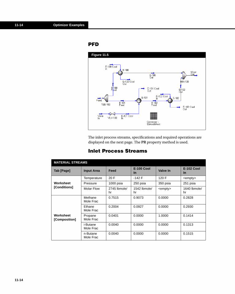
11-14 Optimizer Examples
11-14
PFD
The inlet process streams, specifications and required operations are displayed on the next page. The PR property method is used.
Inlet Process Streams
Figure 11.5
MATERIAL STREAMS
Tab [Page] Input Area FeedE-100 Cool In
Valve InE-102 Cool In
Worksheet [Conditions]
Temperature 20 F -142 F 120 F <empty>
Pressure 1000 psia 250 psia 350 psia 251 psia
Molar Flow 2745 lbmole/hr
1542 lbmole/hr
<empty> 1640 lbmole/hr
Worksheet [Composition]
Methane Mole Frac
0.7515 0.9073 0.0000 0.2828
Ethane Mole Frac
0.2004 0.0927 0.0000 0.2930
Propane Mole Frac
0.0401 0.0000 1.0000 0.1414
i-Butane Mole Frac
0.0040 0.0000 0.0000 0.1313
n-Butane Mole Frac
0.0040 0.0000 0.0000 0.1515

Optimizer 11-15
Process Operations
A tee, valve, mixer and three heat exchangers are required for this process. Input the data as shown in the figures.
Figure 11.6
Figure 11.7
11-15

11-16 Optimizer Examples
11-16
Heat Exchanger E-100
Figure 11.8
HEAT EXCHANGER [E-100]
Tab [Page] Input Area Entry
Design [Parameters]
Tubeside Delta P 10 psia
Shellside Delta P 10 psia
UA 4.00e+04 Btu/F-hr
Heat Loss/Leak None
Heat Exchange Model Weighted
Intervals (E-100 Feed) 10
Intervals (E-100 Cool In) 10
Dew/Bubble Pt (E-100 Cool In)
Inactive
Figure 11.9

Optimizer 11-17
Heat Exchanger E-101
Heat Exchanger E-102
HEAT EXCHANGER [E-101]
Tab [Page] Input Area Entry
Design [Parameters]
Tubeside Delta P 5 psia
Shellside Delta P 1 psia
UA 5.00e+04 Btu/F-hr
Heat Loss/Leak None
Heat Exchange Model Weighted
Intervals (E-100 Feed) 10
Intervals (E-100 Cool In) 10
Figure 11.10
HEAT EXCHANGER [E-102]
Tab [Page] Input Area Entry
Design [Parameters]
Tubeside Delta P 5 psia
Shellside Delta P 5 psia
UA 3.50e+04 Btu/F-hr
Heat Loss/Leak None
Heat Exchange Model Weighted
Intervals (E-100 Feed) 10
Intervals (E-100 Cool In) 10
Dew/Bubble Pt (E-102 Cool In)
Inactive
11-17

11-18 Optimizer Examples
11-18
Stream Specifications• Temperature of stream E-102 Out g -40°F• Vapour Fraction stream E-101 Cool Out g 1.00• Temperature of stream E-100 Out g -65°F• Pressure of E-101 Cool Out g 20 psia• Do not check the Dew/Bubble pt. box for E-101 Cool In or E-
102 Cool In.
Results
The calculated streams are shown below:
Figure 11.11
Figure 11.12
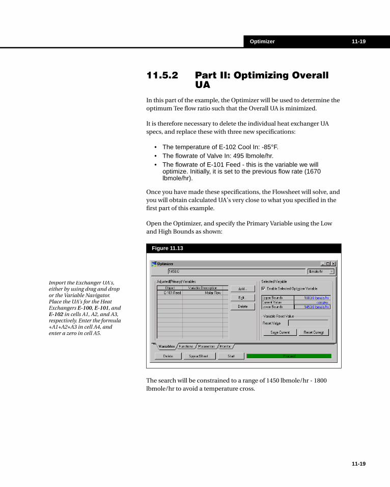
Optimizer 11-19
11.5.2 Part II: Optimizing Overall UA
In this part of the example, the Optimizer will be used to determine the optimum Tee flow ratio such that the Overall UA is minimized.
It is therefore necessary to delete the individual heat exchanger UA specs, and replace these with three new specifications:
• The temperature of E-102 Cool In: -85°F.• The flowrate of Valve In: 495 lbmole/hr.• The flowrate of E-101 Feed - this is the variable we will
optimize. Initially, it is set to the previous flow rate (1670 lbmole/hr).
Once you have made these specifications, the Flowsheet will solve, and you will obtain calculated UA’s very close to what you specified in the first part of this example.
Open the Optimizer, and specify the Primary Variable using the Low and High Bounds as shown:
The search will be constrained to a range of 1450 lbmole/hr - 1800 lbmole/hr to avoid a temperature cross.
Figure 11.13
Import the Exchanger UA’s, either by using drag and drop or the Variable Navigator. Place the UA’s for the Heat Exchangers E-100, E-101, and E-102 in cells A1, A2, and A3, respectively. Enter the formula +A1+A2+A3 in cell A4, and enter a zero in cell A5.
11-19

11-20 Optimizer Examples
11-20
Import the three Heat Exchanger UA’s to the Optimizer SpreadSheet. To do this, press the SpreadSheet button, and select the Spreadsheet tab. Import the information as shown below. In cell A4, enter the formula which will sum the UA’s (Enter the formula +A1+A2+A3). In cell A5, enter 0.0. This will be used in the constraints.
On the Functions tab in the Optimizer property view, it is necessary to define the Objective Function, as well as the Constraint Functions. The Objective Function is the expression we are trying to minimize, which in this case is the sum of the Heat Exchanger UA’s.
Figure 11.14
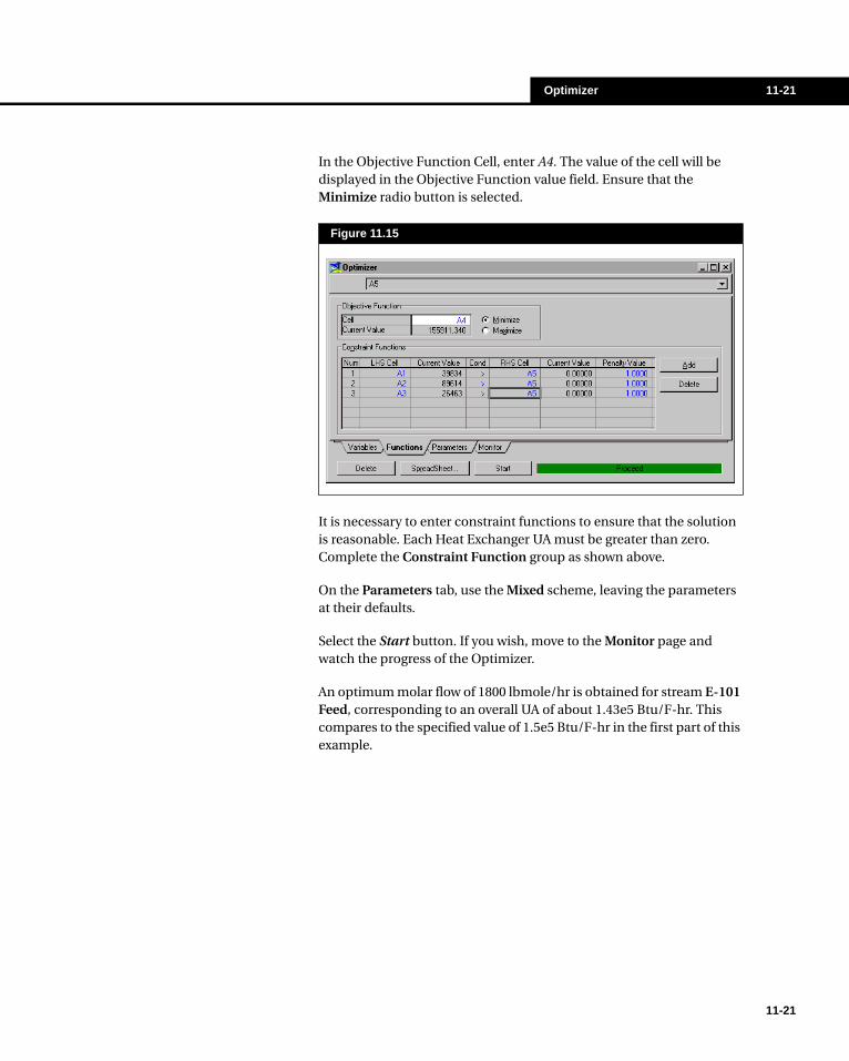
Optimizer 11-21
In the Objective Function Cell, enter A4. The value of the cell will be displayed in the Objective Function value field. Ensure that the Minimize radio button is selected.
It is necessary to enter constraint functions to ensure that the solution is reasonable. Each Heat Exchanger UA must be greater than zero. Complete the Constraint Function group as shown above.
On the Parameters tab, use the Mixed scheme, leaving the parameters at their defaults.
Select the Start button. If you wish, move to the Monitor page and watch the progress of the Optimizer.
An optimum molar flow of 1800 lbmole/hr is obtained for stream E-101 Feed, corresponding to an overall UA of about 1.43e5 Btu/F-hr. This compares to the specified value of 1.5e5 Btu/F-hr in the first part of this example.
Figure 11.15
11-21

11-22 References
11-22
11.6 References 1 Box, M.J. "A New method of Constrained Optimization and a
Comparison with other Methods," Computer J., 8, 42-45, 1965.
2 Press, W.H., et al., "Numerical Recipes in C," Cambridge university Press, 1988.
3 Kuester, J.L. and Mize, J.H., "Optimization Techniques with FORTRAN," McGraw-Hill Book Co., 1973.
4 Harwell Subroutine Library, Release 10, Advanced Computing Dept., AEA Industrial Technology, Harwell laboratory, England, 1990.
5 Powell, M.J.D., "A Fast Algorithm for Non-Linearly Constrained Optimization Calculations," Numerical Analysis, Dundee, 1977, Lecture Notes in Math. 630, Springer-Verlag, 1978.
6 Chamberlain R.M. and Powell, M.J.D., "The Watchdog Technique for Forcing Convergence in Algorithms for Constrained Optimization," Mathematical Programming Study, 16, 1-17, 1982.

Index
A
Absorber Template (Column) 7-17Adiabatic Efficiency 5-11, 5-14, 5-26Adjust 10-3
example 10-13individual 10-13maximum iterations 10-11multiple 10-16solving methods 10-7start 10-12step size 10-10tolerance 10-10
Adjusted Object 10-4Air Cooler 3-3
duty 3-4example 3-9theory 3-3
Annular Mist 4-16
B
Baghouse Filter 8-15parameters 8-16sizing 8-17
Balance 10-17general 10-29heat 10-27mass 10-25mole 10-23mole and heat 10-19types 10-17
Beggs and Brill Correlation 4-14BOX Method (Optimizer Operation) 11-10Broyden Method (Adjust) 10-7
C
Col Dynamic Estimates 7-44Cold Property Specifications (Column) 7-70Column 7-3
3-phase detection 7-10acceleration 7-41advanced solving options 7-30build environment 7-6–7-8composition estimates 7-34–7-35conflicting specifications 7-99conventions 7-15convergence 7-25damping 7-42design tab 7-21dynamics tab 7-69equilibrium error 7-37, 7-100flowsheet tab 7-60flowsheet variables 7-61fluid package 7-4heat and spec error 7-37, 7-38, 7-96, 7-100impossible specifications 7-99initial estimates 7-10inner loop errors 7-95input errors 7-97installation 7-12operations 7-79parameters tab 7-33performance tab 7-52plots 7-53poor initial estimates 7-97property view 7-5rating tab 7-51reactions tab 7-63run / reset buttons 7-21runner 7-20running 7-94–7-95side ops tab 7-47solver 7-4solver tolerance 7-31specification types 7-69specifications 7-69–7-78stream specification 7-78tee 7-92
I-1

I-2
I-2
theory 7-8transfer basis 7-21, 7-60troubleshooting 7-96worksheet tab 7-52
Column Sub-Flowsheet 7-3relationship with main flowsheet 7-6–7-8
ComponentFlow Rate Specification (Column) 7-70Fractions Specification (Column) 7-71Ratio Specification (Column) 7-71Recovery Specification (Column) 7-71
Component Splitter 6-16example 6-20splits page 6-19theory 6-17
Compressor, Centrifugal 5-3curves 5-11–5-13example 5-15isentropic efficiency 5-4solution methods 5-3theory 5-4
Compressor, Reciprocating 5-18example 5-27maximum pressure 5-22piston displacement 5-20rod loading 5-22theory 5-19
Condenser (Column) 7-80duty 7-83pressure drop 7-83subcooling 7-84
Conduction through insulation/pipe 4-26Cooler 3-11
duty 3-13example 3-16pressure drop 3-12theory 3-11zones 3-14
Create Column Stream Spec Button 2-6CSTR 9-4
reactions 9-13Cutpoint Specification (Column) 7-72Cyclone 8-5
constraints 8-8parameters 8-6sizing 8-7solids information 8-6
D
Damping Factorsrecycle 10-46
Delta Temp Specificationcolumn 7-72, 7-73heat exchanger 3-29LNG exchanger 3-56
Distillation Column Template 7-18Dittus and Boelter Correlation 4-24Draw Rate Specification (Column) 7-72Duty Ratio Specification (Column) 7-73Duty Specification
column 7-73heat exchanger 3-30
Dynamic Estimates Integrator 7-44
E
Energy Stream 2-12convert to material stream 2-12
Equilibrium Reactor 9-17Ergun Equation 9-33Examples
3-Phase Separation 6-9air cooler 3-9component splitter 6-20compressor 5-15, 5-27gas cooler 3-16general balance 1 10-31general balance 2 10-32heat balance 10-27heat exchanger 3-46individual adjust 10-13LNG exchanger 3-78mass balance 10-26mixer 4-6mole and heat balance 10-20mole balance 10-23multiple recycle 10-56multiple recycle revisited 10-61optimizer part I 11-13optimizer part II 11-19PFR 9-49pipe segment 4-40pump 5-35relief valve 4-54set 10-66shortcut column 6-14single recycle 10-52
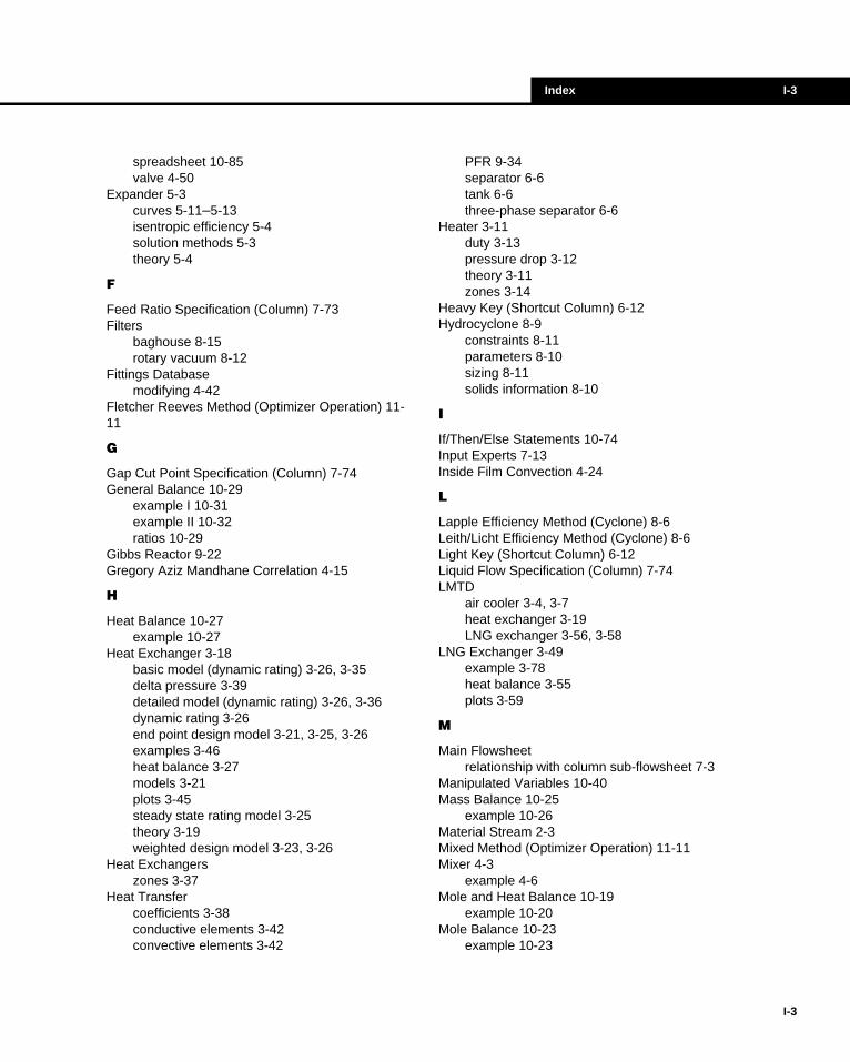
Index I-3
spreadsheet 10-85valve 4-50
Expander 5-3curves 5-11–5-13isentropic efficiency 5-4solution methods 5-3theory 5-4
F
Feed Ratio Specification (Column) 7-73Filters
baghouse 8-15rotary vacuum 8-12
Fittings Databasemodifying 4-42
Fletcher Reeves Method (Optimizer Operation) 11-11
G
Gap Cut Point Specification (Column) 7-74General Balance 10-29
example I 10-31example II 10-32ratios 10-29
Gibbs Reactor 9-22Gregory Aziz Mandhane Correlation 4-15
H
Heat Balance 10-27example 10-27
Heat Exchanger 3-18basic model (dynamic rating) 3-26, 3-35delta pressure 3-39detailed model (dynamic rating) 3-26, 3-36dynamic rating 3-26end point design model 3-21, 3-25, 3-26examples 3-46heat balance 3-27models 3-21plots 3-45steady state rating model 3-25theory 3-19weighted design model 3-23, 3-26
Heat Exchangerszones 3-37
Heat Transfercoefficients 3-38conductive elements 3-42convective elements 3-42
PFR 9-34separator 6-6tank 6-6three-phase separator 6-6
Heater 3-11duty 3-13pressure drop 3-12theory 3-11zones 3-14
Heavy Key (Shortcut Column) 6-12Hydrocyclone 8-9
constraints 8-11parameters 8-10sizing 8-11solids information 8-10
I
If/Then/Else Statements 10-74Input Experts 7-13Inside Film Convection 4-24
L
Lapple Efficiency Method (Cyclone) 8-6Leith/Licht Efficiency Method (Cyclone) 8-6Light Key (Shortcut Column) 6-12Liquid Flow Specification (Column) 7-74LMTD
air cooler 3-4, 3-7heat exchanger 3-19LNG exchanger 3-56, 3-58
LNG Exchanger 3-49example 3-78heat balance 3-55plots 3-59
M
Main Flowsheetrelationship with column sub-flowsheet 7-3
Manipulated Variables 10-40Mass Balance 10-25
example 10-26Material Stream 2-3Mixed Method (Optimizer Operation) 11-11Mixer 4-3
example 4-6Mole and Heat Balance 10-19
example 10-20Mole Balance 10-23
example 10-23
I-3
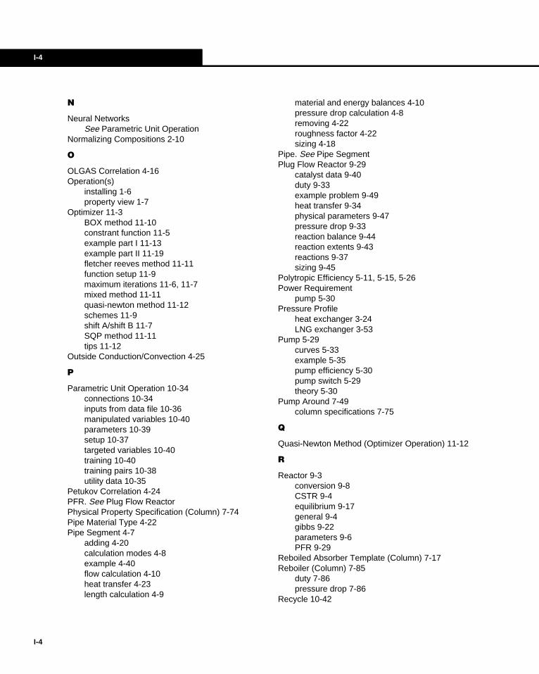
I-4
I-4
N
Neural NetworksSee Parametric Unit Operation
Normalizing Compositions 2-10
O
OLGAS Correlation 4-16Operation(s)
installing 1-6property view 1-7
Optimizer 11-3BOX method 11-10constrant function 11-5example part I 11-13example part II 11-19fletcher reeves method 11-11function setup 11-9maximum iterations 11-6, 11-7mixed method 11-11quasi-newton method 11-12schemes 11-9shift A/shift B 11-7SQP method 11-11tips 11-12
Outside Conduction/Convection 4-25
P
Parametric Unit Operation 10-34connections 10-34inputs from data file 10-36manipulated variables 10-40parameters 10-39setup 10-37targeted variables 10-40training 10-40training pairs 10-38utility data 10-35
Petukov Correlation 4-24PFR. See Plug Flow ReactorPhysical Property Specification (Column) 7-74Pipe Material Type 4-22Pipe Segment 4-7
adding 4-20calculation modes 4-8example 4-40flow calculation 4-10heat transfer 4-23length calculation 4-9
material and energy balances 4-10pressure drop calculation 4-8removing 4-22roughness factor 4-22sizing 4-18
Pipe. See Pipe SegmentPlug Flow Reactor 9-29
catalyst data 9-40duty 9-33example problem 9-49heat transfer 9-34physical parameters 9-47pressure drop 9-33reaction balance 9-44reaction extents 9-43reactions 9-37sizing 9-45
Polytropic Efficiency 5-11, 5-15, 5-26Power Requirement
pump 5-30Pressure Profile
heat exchanger 3-24LNG exchanger 3-53
Pump 5-29curves 5-33example 5-35pump efficiency 5-30pump switch 5-29theory 5-30
Pump Around 7-49column specifications 7-75
Q
Quasi-Newton Method (Optimizer Operation) 11-12
R
Reactor 9-3conversion 9-8CSTR 9-4equilibrium 9-17general 9-4gibbs 9-22parameters 9-6PFR 9-29
Reboiled Absorber Template (Column) 7-17Reboiler (Column) 7-85
duty 7-86pressure drop 7-86
Recycle 10-42
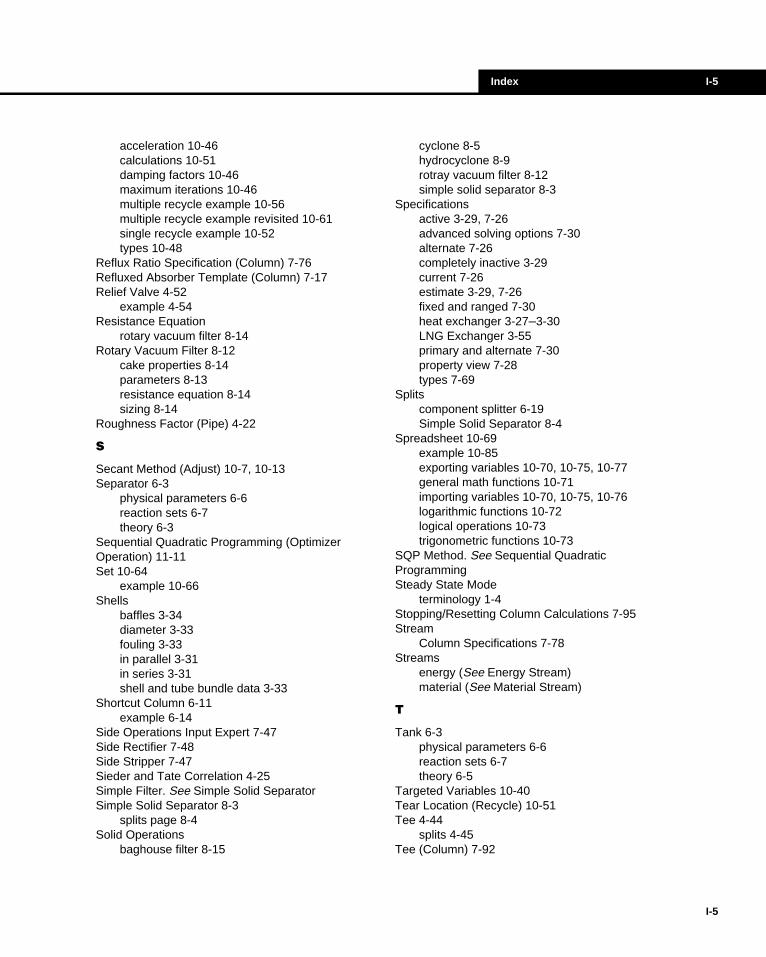
Index I-5
acceleration 10-46calculations 10-51damping factors 10-46maximum iterations 10-46multiple recycle example 10-56multiple recycle example revisited 10-61single recycle example 10-52types 10-48
Reflux Ratio Specification (Column) 7-76Refluxed Absorber Template (Column) 7-17Relief Valve 4-52
example 4-54Resistance Equation
rotary vacuum filter 8-14Rotary Vacuum Filter 8-12
cake properties 8-14parameters 8-13resistance equation 8-14sizing 8-14
Roughness Factor (Pipe) 4-22
S
Secant Method (Adjust) 10-7, 10-13Separator 6-3
physical parameters 6-6reaction sets 6-7theory 6-3
Sequential Quadratic Programming (Optimizer Operation) 11-11Set 10-64
example 10-66Shells
baffles 3-34diameter 3-33fouling 3-33in parallel 3-31in series 3-31shell and tube bundle data 3-33
Shortcut Column 6-11example 6-14
Side Operations Input Expert 7-47Side Rectifier 7-48Side Stripper 7-47Sieder and Tate Correlation 4-25Simple Filter. See Simple Solid SeparatorSimple Solid Separator 8-3
splits page 8-4Solid Operations
baghouse filter 8-15
cyclone 8-5hydrocyclone 8-9rotray vacuum filter 8-12simple solid separator 8-3
Specificationsactive 3-29, 7-26advanced solving options 7-30alternate 7-26completely inactive 3-29current 7-26estimate 3-29, 7-26fixed and ranged 7-30heat exchanger 3-27–3-30LNG Exchanger 3-55primary and alternate 7-30property view 7-28types 7-69
Splitscomponent splitter 6-19Simple Solid Separator 8-4
Spreadsheet 10-69example 10-85exporting variables 10-70, 10-75, 10-77general math functions 10-71importing variables 10-70, 10-75, 10-76logarithmic functions 10-72logical operations 10-73trigonometric functions 10-73
SQP Method. See Sequential Quadratic ProgrammingSteady State Mode
terminology 1-4Stopping/Resetting Column Calculations 7-95Stream
Column Specifications 7-78Streams
energy (See Energy Stream)material (See Material Stream)
T
Tank 6-3physical parameters 6-6reaction sets 6-7theory 6-5
Targeted Variables 10-40Tear Location (Recycle) 10-51Tee 4-44
splits 4-45Tee (Column) 7-92
I-5

I-6
I-6
Tee Split Fraction Specification (Column) 7-76Templates
3 sidestripper crude column 7-134 sidestripper crude column 7-13absorber 7-17column 7-14–7-20distillation 7-18FCCU main fractionator 7-13liquid-liquid extractor 7-13reboiled absorber 7-17refluxed absorber 7-17three phase distillation 7-13wet vacuum tower 7-13
Three Phase Distillationdetection of three phases 7-10three phase theory 7-9
Three-Phase Separator 6-3example 6-9physical parameters 6-6reaction sets 6-7theory 6-3
Training 10-40Training Pairs 10-38Transport Property Specifications (Column) 7-77Tray Section (Column) 7-87
connections page 7-88parameters page 7-89performance page 7-92pressures page 7-91side draws page 7-89
Tray Temperature Specification (Column) 7-76Tubes (Heat Exchanger) 3-34
dimensions 3-34heat transfer length 3-34
U
UAheat exchanger 3-24LNG exchanger 3-56, 3-58
User Property Specification (Column) 7-77Utility Data 10-35
V
Valve 4-48example 4-50
Vapor Flow Specification (Column) 7-77Vapour Fraction Specification (Column) 7-78Vapour Pressure Specifications (Column) 7-78
W
Wave Flow (Pipe Segment) 4-15Wegstein Count
recycle 10-45, 10-47
Z
Zonescooler/heater 3-14heat exchanger 3-37