2.4 The giant component of the Erdos–Renyi random graph

2.4.1 Non-rigorous discussion

We know that if pn = o(1) then there are no triangles. In a similar manner it can be shown thatthere are no cycles of any order in G(n, p). This means that most components of the randomgraph are trees and isolated vertices. For p > c log n/n for c ≥ 1 the random graph is connecteda.a.s. What happens in between these stages? It turns our that a unique giant componentappears when p = c/n, c > 1. We first study the appearance of this largest component in aheuristic manner. We define the giant component as the component of G(n, p), whose order isO(n).

Let u be the frequency of the vertices that do not belong to the giant component. In otherwords, u gives the probability that a randomly picked vertex does not belong to the giantcomponent. Let us calculate this probability in a different way. Pick any other vertex. Itcan be either in the giant component or not. For the original node not to belong to the giantcomponent these two either should not be connected (probability 1 − p) or be connected, butthe latter vertex is not in the giant component (probability pu). There are n − 1 vertices tocheck, hence

u = (1− p+ pu)n−1.

Recall that we are dealing with pn ∼ λ, hence it is convenient to use the parametrization

p =λ

n, λ > 0.

Note that λ is the mean degree of G(n, p). We get

u =

(

1− λ

n(1− u)

)n−1

=⇒

log u(n − 1) log

(

1− λ

n(1− u)

)

=⇒

log u ≈ −λ(n− 1)

n(1− u) =⇒

log u ≈ −λ(1− u) =⇒u = e−λ(1−u),

where the fact that log(1 + x) ≈ x for small x was used.Finally, for the frequency of the vertices in the giant component v = 1− u we obtain

1− v = e−λv.

This equation always has the solution v = 0. However, this is not the only solution for allpossible λs. To see this consider two curves, defined by f(v) = 1 − e−λv and g(v) = v. Theirintersections give the roots to the original equation. Note that, as expected, f(0) = g(0) = 0.Note also that f ′(v) = λe−λv > 0 and f ′′(v) = −λ2e−λv < 0. Hence the derivative for v ≤ 0cannot be bigger than at v = 0, which is f ′(0) = λ. Hence (see the figure), if λ ≤ 0 then thereis unique trivial solution v = 0, but if λ > 1 then another positive solution 0 < v < 1 appears.

36

0

v

v

f(v)

λ > 1

λ = 1

λ < 1

0 1 2 3

0

1

λ

v(λ)

Figure 2.1: The analysis of the number of solutions of the equation 1− v = e−λv . The left panelshows that if v ≥ 0 then it is possible to have one trivial solution v = 0 in the case λ ≤ 1, andtwo solutions if λ > 1. The right panel shows the solutions (thick curves) as the functions of λ

Technically, we only showed that if λ ≤ 1 then there is no giant component. If λ > 1 thenwe use the following argument. Since λ gives the mean degree, then, starting from a randomlypicked vertex, it will have λ neighbors on average. Its neighbors will have λ2 neighbors (thereare λ of them and each has λ adjacent edges) and so on. After s steps we would have λs verticeswithin the distance s from the initial vertex. If λ > 1 this number will grow exponentially andhence most of the nodes have to be connected into the giant component. Their frequency canbe found as the nonzero solution to 1− v = e−λv. Of course this type of argument is extremelyrough, but the fact is that it can be made absolutely rigorous within the framework of thebranching processes.

Moreover, the last heuristic reasoning can be used to estimate the diameter of G(n, p). Ob-viously, the process of adding new vertices cannot continue infinitely, it has to stop when wereach all n vertices:

λs = n.

From where we have that

s =log n

log λ

approximates the diameter of the Erdos–Renyi random graph. It is quite surprising that theexact results are basically the same: It can be proved that for np > 1 and np < c log n, thediameter of the random graph (understood as the diameter of the largest connected component)is concentrated on at most four values around log n/ log np.

Finally we note that since the appearance of the giant component shows this thresholdbehavior (if λ < 1 there is no giant component a.a.s., if λ > 1 the giant component is presenta.a.s.) one often speaks of a phase transition.

2.4.2 Rigorous results for the appearance of the giant component

Add the discussion on the branching processes

and relation to the appearance of the giant component.

37

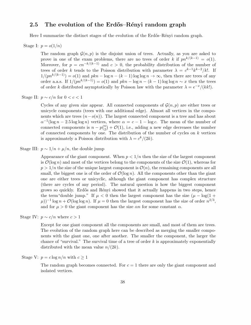
2.5 The evolution of the Erdos–Renyi random graph

Here I summarize the distinct stages of the evolution of the Erdos–Renyi random graph.

Stage I: p = o(1/n)

The random graph G(n, p) is the disjoint union of trees. Actually, as you are asked toprove in one of the exam problems, there are no trees of order k if pnk/(k−1) = o(1).Moreover, for p = cn−k/(k−1) and c > 0, the probability distribution of the number oftrees of order k tends to the Poisson distribution with parameter λ = ck−1kk−2/k!. If1/(pnk/(k−1)) = o(1) and pkn− log n− (k − 1) log log n → ∞, then there are trees of anyorder a.a.s. If 1/(pnk/(k−1)) = o(1) and pkn − log n − (k − 1) log log n ∼ x then the treesof order k distributed asymptotically by Poisson law with the parameter λ = e−x/(kk!).

Stage II: p ∼ c/n for 0 < c < 1

Cycles of any given size appear. All connected components of G(n, p) are either trees orunicycle components (trees with one additional edge). Almost all vertices in the compo-nents which are trees (n−o(n)). The largest connected component is a tree and has aboutα−1(log n − 2.5 log log n) vertices, where α = c − 1 − log c. The mean of the number ofconnected components is n − p

(n2

)

+ O(1), i.e., adding a new edge decreases the numberof connected components by one. The distribution of the number of cycles on k verticesis approximately a Poisson distribution with λ = ck/(2k).

Stage III: p ∼ 1/n + µ/n, the double jump

Appearance of the giant component. When p < 1/n then the size of the largest componentis O(log n) and most of the vertices belong to the components of the size O(1), whereas forp > 1/n the size of the unique largest component is O(n), the remaining components are allsmall, the biggest one is of the order of O(log n). All the components other than the giantone are either trees or unicyclic, although the giant component has complex structure(there are cycles of any period). The natural question is how the biggest componentgrows so quickly. Erdos and Renyi showed that it actually happens in two steps, hencethe term“double jump.” If µ < 0 then the largest component has the size (µ − log(1 +µ))−1 log n+O(log log n). If µ = 0 then the largest component has the size of order n2/3,and for µ > 0 the giant component has the size αn for some constant α.

Stage IV: p ∼ c/n where c > 1

Except for one giant component all the components are small, and most of them are trees.The evolution of the random graph here can be described as merging the smaller compo-nents with the giant one, one after another. The smaller the component, the larger thechance of “survival.” The survival time of a tree of order k is approximately exponentiallydistributed with the mean value n/(2k).

Stage V: p = c log n/n with c ≥ 1

The random graph becomes connected. For c = 1 there are only the giant component andisolated vertices.

38

Stage VI: p = ω(n) log n/n where ω(n) → ∞ as n → ∞. In this range the random graph is not onlyconnected, but also the degrees of all the vertices are asymptotically equal.

Here is the numerical illustration of the evolution of the random graph. To present it I fixedn = 1000 the number of vertices and generated

(n2

)

random variables, uniformly distributed in[0, 1]. Hence each edge gets its only number pj ∈ [0, 1], j = 1, . . . ,

(n2

)

. For any fixed p ∈ (0, 1) Idraw only the edges for which pj ≤ p. Therefore, in this manner I can observe how the evolutionof the random graph occurs for G(n, p).

39

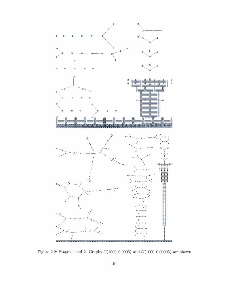
Figure 2.2: Stages 1 and 2. Graphs G(1000, 0.0005) and G(1000, 0.00095) are shown

40

Figure 2.3: Stages 3 and 4. Graphs G(1000, 0.001) and G(1000, 0.0015) are shown. The giantcomponent is born

41

Figure 2.4: Stages 4 and 5. Graphs G(1000, 0.004) and G(1000, 0.007) are shown. The finalgraph is connected (well, almost)

42

Chapter 3

Generalizations of the Erdos–Renyi

random graphs

3.1 Introduction

3.2 Generating functions

3.3 Configuration model

43