Embed Size (px)
Citation preview
24-02-2006 Siddhartha Shakya 1
Estimation Of Distribution Algorithm based on Markov
Random Fields
Siddhartha ShakyaSchool Of Computing
The Robert Gordon University

24-02-2006 Siddhartha Shakya 2
Outline• From GAs to EDAs
• Probabilistic Graphical Models in EDAs– Bayesian networks
– Markov Random Fields
• Fitness modelling approach to estimating and sampling MRF in EDA– Gibbs distribution, energy function and modelling the
fitness
– Estimating parameters (Fitness modelling approach)
– Sampling MRF (several different approaches)
• Conclusion

24-02-2006 Siddhartha Shakya 3
Genetic Algorithms (GAs)• Population based optimisation technique
• Based on Darwin's theory of Evolution
• A solution is encoded as a set of symbols known as chromosome
• A population of solution is generated
• Genetic operators are then applied to the population to get next generation that replaces the parent population

24-02-2006 Siddhartha Shakya 4
Simple GA simulation

24-02-2006 Siddhartha Shakya 5
GA to EDA

24-02-2006 Siddhartha Shakya 6
Simple EDA simulation
n
iixpxp
1
)()(
0 1 1 1 1
1 0 1 0 1
0 0 1 0 1
0 1 0 0 0
0 1 1 1 1
1 0 1 0 1
0 0 1 0 1
0 1 0 0 0
0.5 0.5 1.0 1.00.5
0 0 1 1 1
1 1 1 0 1
1 0 1 0 1
0 1 1 1 1
)1( 5 xp
24-02-2006 Siddhartha Shakya 7
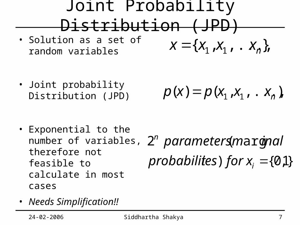
Joint Probability Distribution (JPD)• Solution as a set of
random variables
• Joint probability Distribution (JPD)
• Exponential to the number of variables, therefore not feasible to calculate in most cases
• Needs Simplification!!
},...,,{ 11 nxxxx
),...,,()( 11 nxxxpxp
}1,0{)
arg(2
i
n
xforiesprobabilit
inalmparameters

24-02-2006 Siddhartha Shakya 8
Factorisation of JPD
• Univariate model: No interaction: Simplest model
• Bivariate model: Pair-wise interaction
• Multivariate Model: interaction of more than two variables
xxxpxp i
n
ii
:)()(1
xxxxxpxp ji
n
iji
,:)|()(1
xxxxxxpxp Ai
n
iAi
,:)|()(1
24-02-2006 Siddhartha Shakya 9
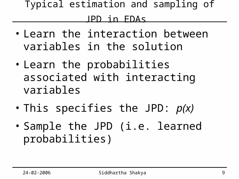
Typical estimation and sampling of JPD in EDAs
• Learn the interaction between variables in the solution
• Learn the probabilities associated with interacting variables
• This specifies the JPD: p(x)
• Sample the JPD (i.e. learned probabilities)
24-02-2006 Siddhartha Shakya 10
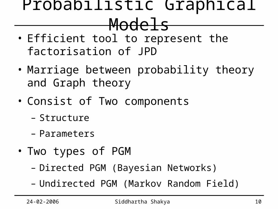
Probabilistic Graphical Models• Efficient tool to represent the factorisation of
JPD
• Marriage between probability theory and Graph theory
• Consist of Two components
– Structure
– Parameters
• Two types of PGM
– Directed PGM (Bayesian Networks)
– Undirected PGM (Markov Random Field)
24-02-2006 Siddhartha Shakya 11
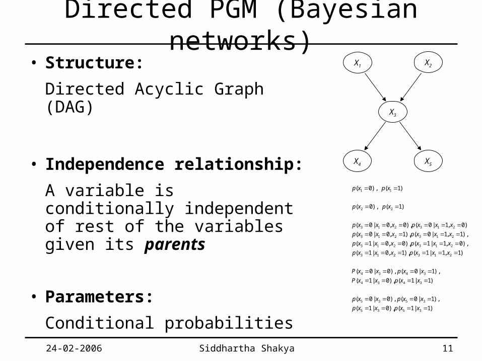
Directed PGM (Bayesian networks)• Structure:
Directed Acyclic Graph (DAG)
• Independence relationship:
A variable is conditionally independent of rest of the variables given its parents
• Parameters:
Conditional probabilities
X1 X2
X3
X4 X5
)1|1(),0|1(
),1|0(),0|0(
)1|1(),0|1(
),1|0(),0|0(
)1,1|1(),1,0|1(
),0,1|1(),0,0|1(
),1,1|0(),1,0|0(
),0,1|0(),0,0|0(
)1(),0(
)1(),0(
3535
3535
3434
3434
213213
213213
213213
213213
22
11
xxpxxp
xxpxxp
xxpxxP
xxpxxP
xxxpxxxp
xxxpxxxp
xxxpxxxp
xxxpxxxp
xpxp
xpxp

24-02-2006 Siddhartha Shakya 12
Bayesian networks• The factorisation of JPD
encoded in terms of conditional probabilities is
• JPD for BN
X1 X2
X3
X4 X5
)1|1(),0|1(
),1|0(),0|0(
)1|1(),0|1(
),1|0(),0|0(
)1,1|1(),1,0|1(
),0,1|1(),0,0|1(
),1,1|0(),1,0|0(
),0,1|0(),0,0|0(
)1(),0(
)1(),0(
3535
3535
3434
3434
213213
213213
213213
213213
22
11
xxpxxp
xxpxxp
xxpxxP
xxpxxP
xxxpxxxp
xxxpxxxp
xxxpxxxp
xxxpxxxp
xpxp
xpxp
n
iiixpxp
1
)|()(
)|()|(),|()()()( 353421321 xxpxxpxxxpxpxpxp

24-02-2006 Siddhartha Shakya 13
Estimating a Bayesian network• Estimate structure
• Estimate parameters
• This completely specifies the JPD
• JPD can then be Sampled
)1|1(),0|1(
),1|0(),0|0(
)1|1(),0|1(
),1|0(),0|0(
)1,1|1(),1,0|1(
),0,1|1(),0,0|1(
),1,1|0(),1,0|0(
),0,1|0(),0,0|0(
)1(),0(
)1(),0(
3535
3535
3434
3434
213213
213213
213213
213213
22
11
xxpxxp
xxpxxp
xxpxxP
xxpxxP
xxxpxxxp
xxxpxxxp
xxxpxxxp
xxxpxxxp
xpxp
xpxp
)|()|(),|()()()( 353421321 xxpxxpxxxpxpxpxp
X1 X2
X3
X4 X5
24-02-2006 Siddhartha Shakya 14
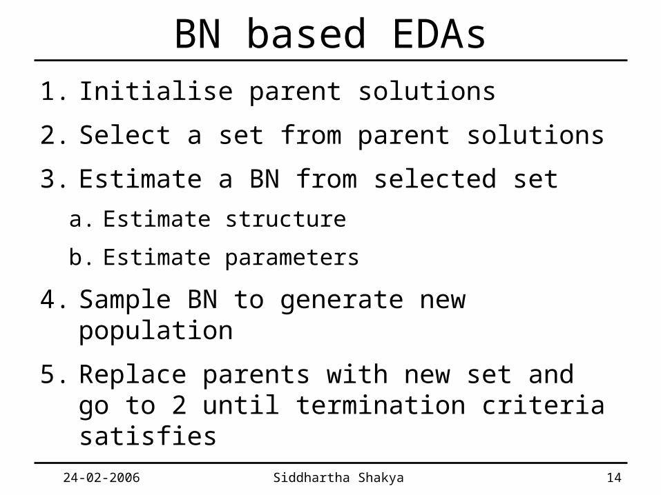
BN based EDAs1. Initialise parent solutions
2. Select a set from parent solutions
3. Estimate a BN from selected set
a. Estimate structure
b. Estimate parameters
4. Sample BN to generate new population
5. Replace parents with new set and go to 2 until termination criteria satisfies

24-02-2006 Siddhartha Shakya 15
How to estimate and sample BN in EDAs
• Estimating structure
– Score + Search techniques
– Conditional independence test
• Estimating parameters
– Trivial in EDAs: Dataset is complete
– Estimate probabilities of parents before child
• Sampling
– Probabilistic Logical Sampling (Sample parents before child)
X1 X2
X3
X4 X5
)|()|(),|()()()( 353421321 xxpxxpxxxpxpxpxp
24-02-2006 Siddhartha Shakya 16
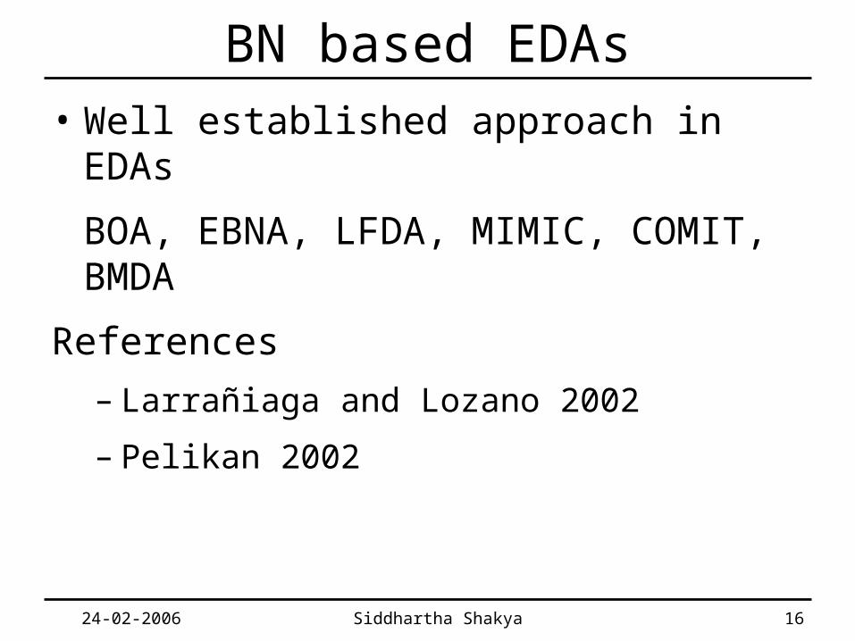
BN based EDAs• Well established approach in EDAs
BOA, EBNA, LFDA, MIMIC, COMIT, BMDA
References
– Larrañiaga and Lozano 2002
– Pelikan 2002

24-02-2006 Siddhartha Shakya 17
Markov Random Fields (MRF)• Structure:
Undirected Graph
• Local independence:
A variable is conditionally independent of rest of the variables given its neighbours
• Global Independence:
Two sets of variables are conditionally independent to each other if there is a third set that separates them.
• Parameters:
potential functions defined on the cliques
X1
X3X2
X4 X6X5
),(
),(
),,(
),,(
634
523
4322
3211
xx
xx
xxx
xxx

24-02-2006 Siddhartha Shakya 18
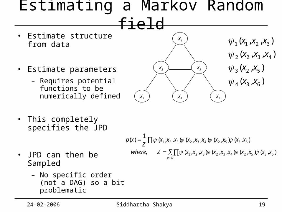
Markov Random Field• The factorisation of JPD
encoded in terms of potential function over maximal cliques is
• JPD for MRF
),(
),(
),,(
),,(
634
523
4322
3211
xx
xx
xxx
xxx
X1
X3X2
X4 X6X5
functionpartitionais
xxxxxxxxxxZwhere
xxxxxxxxxxZ
xp
x
),(),(),,(),,(,
),(),(),,(),,(1
)(
6352432321
6352432321
m
iic
Zxp
1
)(1
)(
24-02-2006 Siddhartha Shakya 19
Estimating a Markov Random field• Estimate structure from
data
• Estimate parameters
– Requires potential functions to be numerically defined
• This completely specifies the JPD
• JPD can then be Sampled
– No specific order (not a DAG) so a bit problematic
X1
X3X2
X4 X6X5
),(
),(
),,(
),,(
634
523
4322
3211
xx
xx
xxx
xxx
x
xxxxxxxxxxZwhere
xxxxxxxxxxZ
xp
),(),(),,(),,(,
),(),(),,(),,(1
)(
6352432321
6352432321

24-02-2006 Siddhartha Shakya 20
MRF in EDA• Has recently been proposed as a
estimation of distribution technique in EDA
• Shakya et al 2004, 2005
• Santana et el 2003, 2005
24-02-2006 Siddhartha Shakya 21
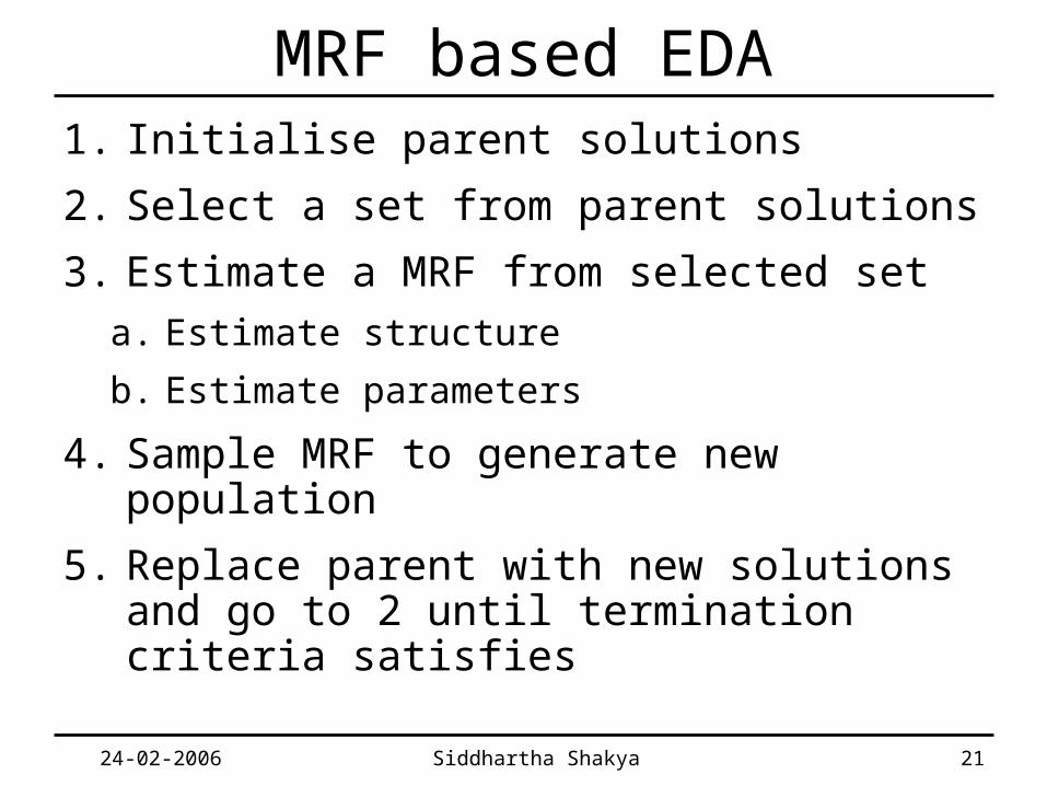
MRF based EDA1. Initialise parent solutions
2. Select a set from parent solutions
3. Estimate a MRF from selected set
a. Estimate structure
b. Estimate parameters
4. Sample MRF to generate new population
5. Replace parent with new solutions and go to 2 until termination criteria satisfies

24-02-2006 Siddhartha Shakya 22
How to estimate and sample MRF in EDA
• Learning Structure– Conditional Independence test (MN-EDA, MN-FDA)
– Linkage detection algorithm (LDFA)
• Learning Parameter– Junction tree approach (FDA)
– Junction graph approach (MN-FDA)
– Kikuchi approximation approach (MN-EDA)
– Fitness modelling approach (DEUM)
• Sampling– Probabilistic Logic Sampling (FDA, MN-FDA)
– Probability vector approach (DEUMpv)
– Direct sampling of Gibbs distribution (DEUMd)
– Metropolis sampler (Is-DEUMm)
– Gibbs Sampler (Is-DEUMg, MN-EDA)

24-02-2006 Siddhartha Shakya 23
Fitness modelling approach• Hamersley Clifford theorem: JPD for
any MRF follows Gibbs distribution
• Energy of Gibbs distribution in terms of potential functions over the cliques
• Assuming probability of solution is proportional to its fitness:
• From (a) and (b) a Model of fitness function - MRF fitness model (MFM) – is derived
)()(/)(
aZ
exp
TxU
m
iicuxU
1
)()(
)()(
)( bZ
xfxp
)())(ln( xUxf
m
iicuxf
1
)())(ln(
,or

24-02-2006 Siddhartha Shakya 24
MRF fitness Model (MFM)
• Properties:
– Completely specifies the JPD for MRF
– Negative relationship between fitness and Energy i.e. Minimising energy = maximise fitness
• Task:
– Need to find the structure for MRF
– Need to numerically define clique potential function
m
iicuxUxf
1
)()())(ln(

24-02-2006 Siddhartha Shakya 25
MRF Fitness Model (MFM)• Let us start with simplest model:
univariate model – this eliminates structure learning :)
• For univariate model there will be n singleton clique
• For each singleton clique assign a potential function
• Corresponding MFM
• In terms of Gibbs distribution
iiii xxu )(
X1
X3X2
X4 X6X5
)(
)(
)(
)(
)(
)(
66
55
44
33
22
11
xu
xu
xu
xu
xu
xu
nn xxxxUxf ..)())(ln( 2211
Z
exp
Txm
iii
1
)(

24-02-2006 Siddhartha Shakya 26
Estimating MRF parameters using MFM
• Each chromosome gives us a linear equation
• Applying it to a set of selected solution gives us a system of linear equations
• Solving it will give us the approximation to the MRF parameters
• Knowing MRF parameters completely specifies JPD
• Next step is to sample the JPD
nn xxxxf ..))(ln( 2211

24-02-2006 Siddhartha Shakya 27
General DEUM frameworkDistribution Estimation Using MRF algorithm
(DEUM)
1. Initialise parent population P
2. Select set D from P (can use D=P !!)
3. Build a MFM and fit to D to estimate MRF parameters
4. Sample MRF to generate new population
5. Replace P with new population and go to 2 until termination criterion satisfies

24-02-2006 Siddhartha Shakya 28
How to sample MRF• Probability vector approach
• Direct Sampling of Gibbs Distribution
• Metropolis sampling
• Gibbs sampling

24-02-2006 Siddhartha Shakya 29
Probability vector approach to sample MRF
• Minimise U(x) to maximise f(x)
• To minimise U(x) Each αixi should be minimum
• This suggests: if αi is negative then corresponding xi
should be positive
• We could get an optimum chromosome for the current population just by looking on α
• However not always the current population contains enough information to generate optimum
• We look on sign of each αi to update a vector of probability
nn xxxxUxf ..)())(ln( 2211

24-02-2006 Siddhartha Shakya 30
DEUM with probability vector (DEUMpv)
24-02-2006 Siddhartha Shakya 31
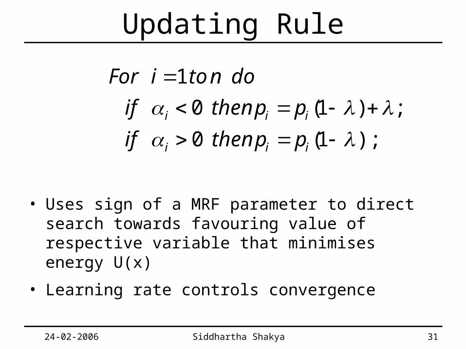
Updating Rule
• Uses sign of a MRF parameter to direct search towards favouring value of respective variable that minimises energy U(x)
• Learning rate controls convergence
);1(0
;)1(0
1
iii
iii
ppthenif
ppthenif
dontoiFor
24-02-2006 Siddhartha Shakya 32
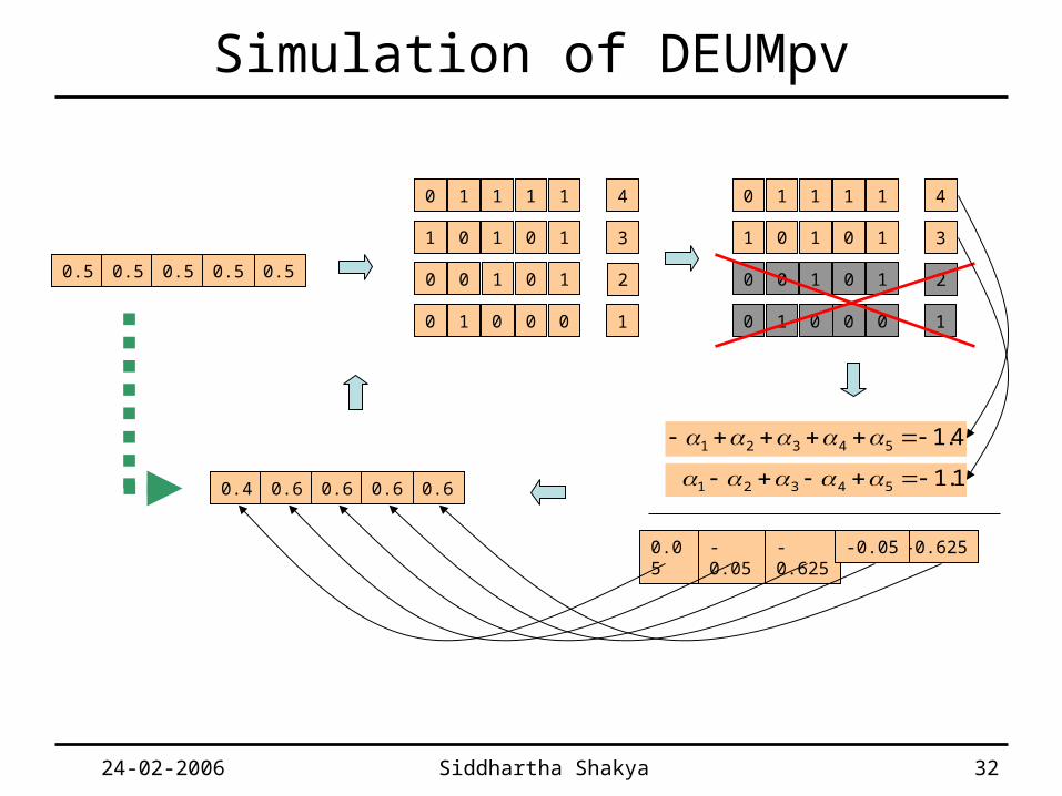
Simulation of DEUMpv
0 1 1 1 1
1 0 1 0 1
0 0 1 0 1
0 1 0 0 0
0.4 0.6 0.6 0.60.6
0.5 0.5 0.5 0.50.5
4
3
2
1
0 1 1 1 1
1 0 1 0 1
4
3
0 0 1 0 1
0 1 0 0 0
2
1
4.154321
1.154321
0.05 -0.05 -0.625 -0.625-0.05
24-02-2006 Siddhartha Shakya 33
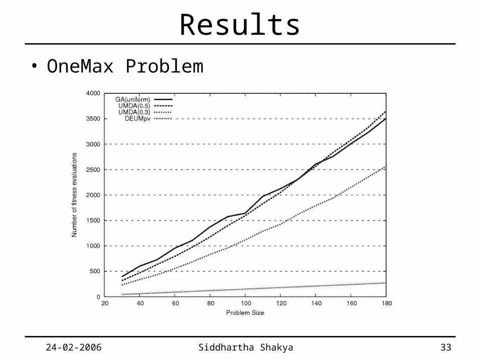
Results• OneMax Problem
24-02-2006 Siddhartha Shakya 34
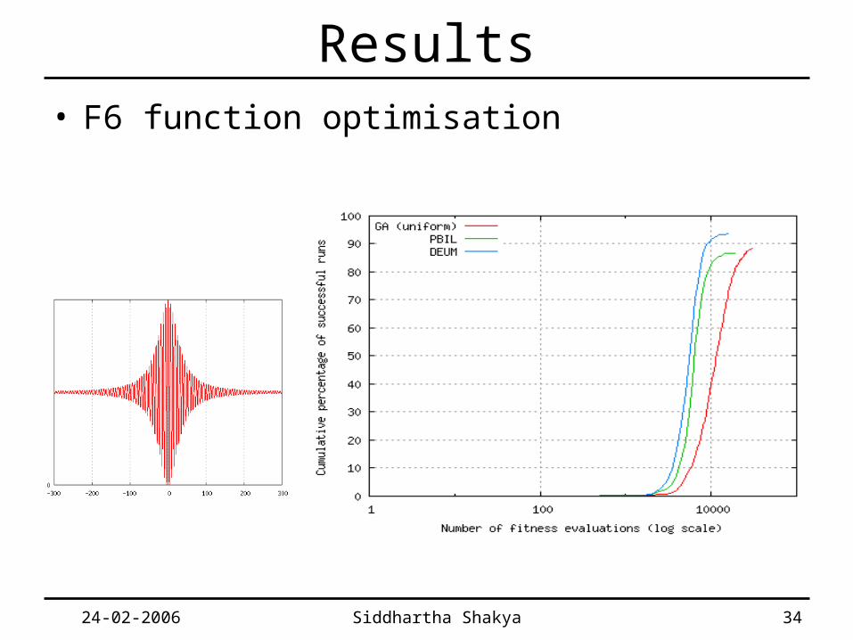
Results• F6 function optimisation

24-02-2006 Siddhartha Shakya 35
Results• Trap 5 function
• Deceptive problem
• No solution found
24-02-2006 Siddhartha Shakya 36
Sampling MRF• Probability vector approach
• Direct sampling of Gibbs distribution
• Metropolis sampling
• Gibbs sampling
24-02-2006 Siddhartha Shakya 37
Direct Sampling of Gibbs distribution
• In the probability vector approach, only the sign of MRF parameters has been used
• However, one could directly sample from the Gibbs distribution and make use of the values of MRF parameters
• Also could use the temperature coefficient to manipulate the probabilities

24-02-2006 Siddhartha Shakya 38
Direct Sampling of Gibbs distribution
nn
TxU
xxxxUZ
exp
..)()( 2211
)(
TxxUTxxU
TxxU
x
ii ii
i
i
ee
e
xp
xxpxp /)1)((/)1)((
/)1)((
}1,1{
)(
1)()1(
Ti iexp /21
1)1( Ti ie
xp /21
1)1(
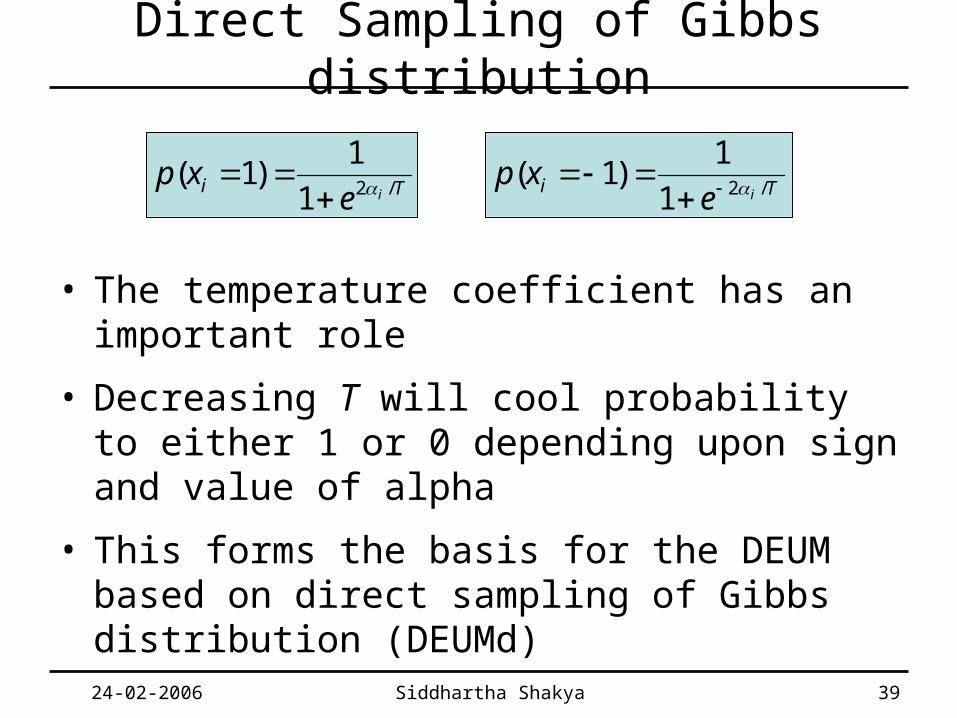
24-02-2006 Siddhartha Shakya 39
Direct Sampling of Gibbs distribution
• The temperature coefficient has an important role
• Decreasing T will cool probability to either 1 or 0 depending upon sign and value of alpha
• This forms the basis for the DEUM based on direct sampling of Gibbs distribution (DEUMd)
Ti iexp /21
1)1( Ti ie
xp /21
1)1(
24-02-2006 Siddhartha Shakya 40
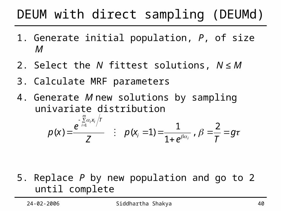
DEUM with direct sampling (DEUMd)
1. Generate initial population, P, of size M
2. Select the N fittest solutions, N ≤ M
3. Calculate MRF parameters
4. Generate M new solutions by sampling univariate distribution
5. Replace P by new population and go to 2 until complete
gTe
xpZ
exp
i
m
iii
i
Tx
2
,1
1)1()(
1
24-02-2006 Siddhartha Shakya 41
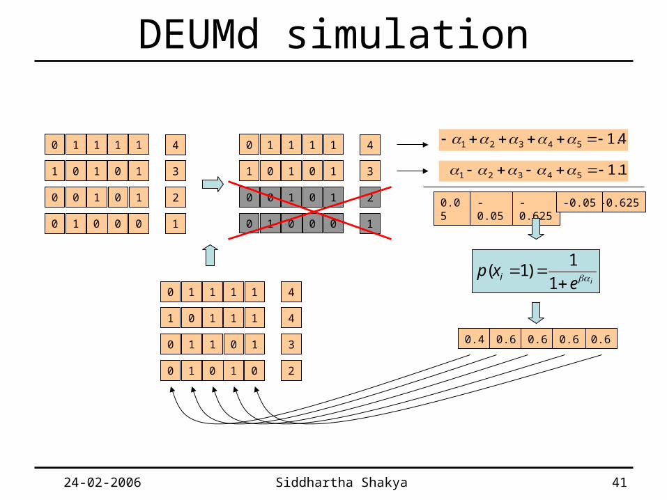
DEUMd simulation
4.154321 0 1 1 1 1
1 0 1 0 1
0 0 1 0 1
0 1 0 0 0
4
3
2
1
0 1 1 1 1
1 0 1 0 1
4
3
0 0 1 0 1
0 1 0 0 0
2
1
1.154321
0.05 -0.05 -0.625 -0.625-0.05
iexp i
1
1)1(
0.4 0.6 0.6 0.60.6
0 1 1 1 1
1 0 1 1 1
0 1 1 0 1
0 1 0 1 0
4
4
3
2

24-02-2006 Siddhartha Shakya 42
Experimental results• OneMax Problem

24-02-2006 Siddhartha Shakya 43
F6 function optimization

24-02-2006 Siddhartha Shakya 44
Plateau Problem (n=180)

24-02-2006 Siddhartha Shakya 45
Checker Board Problem (n=100)
24-02-2006 Siddhartha Shakya 46
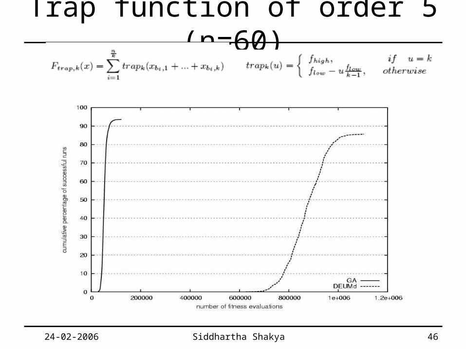
Trap function of order 5 (n=60)
24-02-2006 Siddhartha Shakya 47
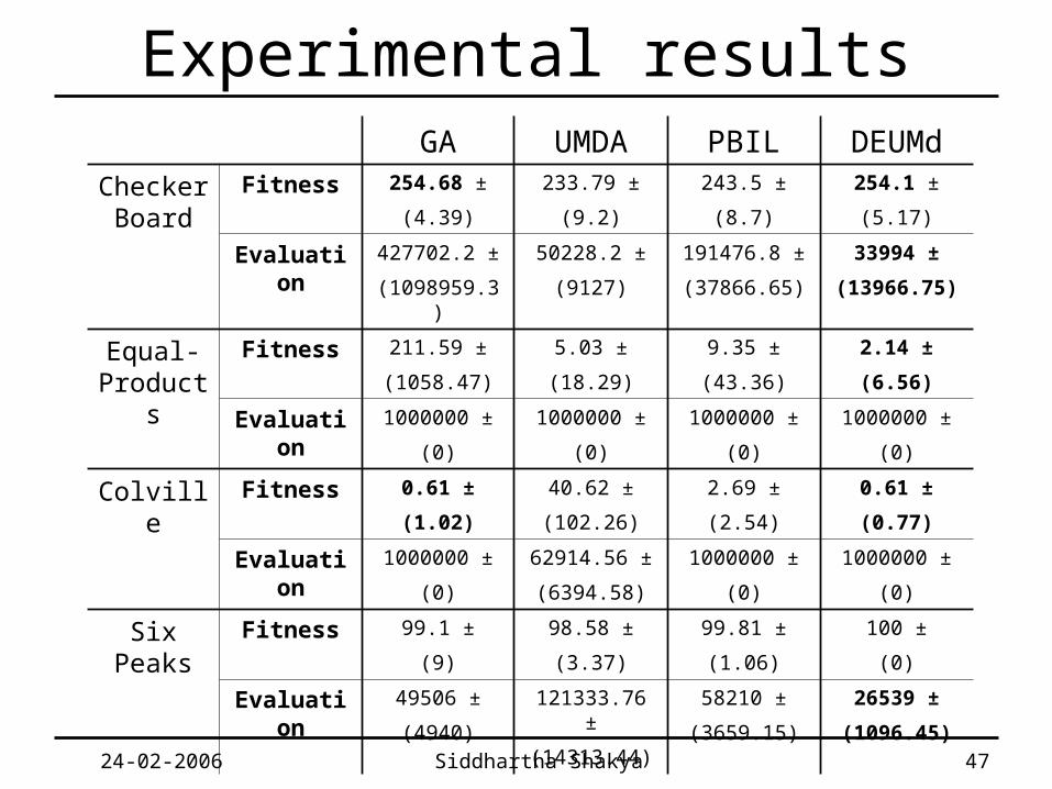
Experimental resultsGA UMDA PBIL DEUMd
Checker Board
Fitness 254.68 ±
(4.39)
233.79 ±
(9.2)
243.5 ±
(8.7)
254.1 ±
(5.17)
Evaluation 427702.2 ±
(1098959.3)
50228.2 ±
(9127)
191476.8 ±
(37866.65)
33994 ±
(13966.75)
Equal-Products
Fitness 211.59 ±
(1058.47)
5.03 ±
(18.29)
9.35 ±
(43.36)
2.14 ±
(6.56)
Evaluation 1000000 ±
(0)
1000000 ±
(0)
1000000 ±
(0)
1000000 ±
(0)
Colville Fitness 0.61 ±
(1.02)
40.62 ±
(102.26)
2.69 ±
(2.54)
0.61 ±
(0.77)
Evaluation 1000000 ±
(0)
62914.56 ±
(6394.58)
1000000 ±
(0)
1000000 ±
(0)
Six Peaks
Fitness 99.1 ±
(9)
98.58 ±
(3.37)
99.81 ±
(1.06)
100 ±
(0)
Evaluation 49506 ±
(4940)
121333.76 ±
(14313.44)
58210 ±
(3659.15)
26539 ±
(1096.45)

24-02-2006 Siddhartha Shakya 48
Analysis of Results• For Univariate problems (OneMax), given population size of 1.5n,
P=D and T->0, solution was found in single generation
• For problems with low order dependency between variables (Plateau and CheckerBoard), performance was significantly better than that of other Univariate EDAs.
• For the deceptive problems with higher order dependency (Trap function and Six peaks) DEUMd was deceived but by slowing the cooling rate, it was able to find solution for Trap of order 5.
• For the problems where optimum was not known the performance was comparable to that of GA and other EDAs and was better in some cases.

24-02-2006 Siddhartha Shakya 49
Cost- Benefit Analysis (the cost)• Polynomial cost of estimating the distribution
compared to linear cost of other univariate EDAs
nNnNO
nNNnO
nNnO
)(
)(
)(
2
2
3
• Cost to compute univariate marginal frequency:
)(nNO
• Cost to compute SVD

24-02-2006 Siddhartha Shakya 50
Cost- Benefit Analysis (the benefit)
• DEUMd can significantly reduce the number of fitness evaluations
• Quality of solution was better for DEUMd than other compared EDAs
• DEUMd should be tried on problems where the increased solution quality outweigh computational cost.
24-02-2006 Siddhartha Shakya 51
Sampling MRF• Probability vector approach
• Direct Sampling of Gibbs Distribution
• Metropolis sampling
• Gibbs sampling
24-02-2006 Siddhartha Shakya 52
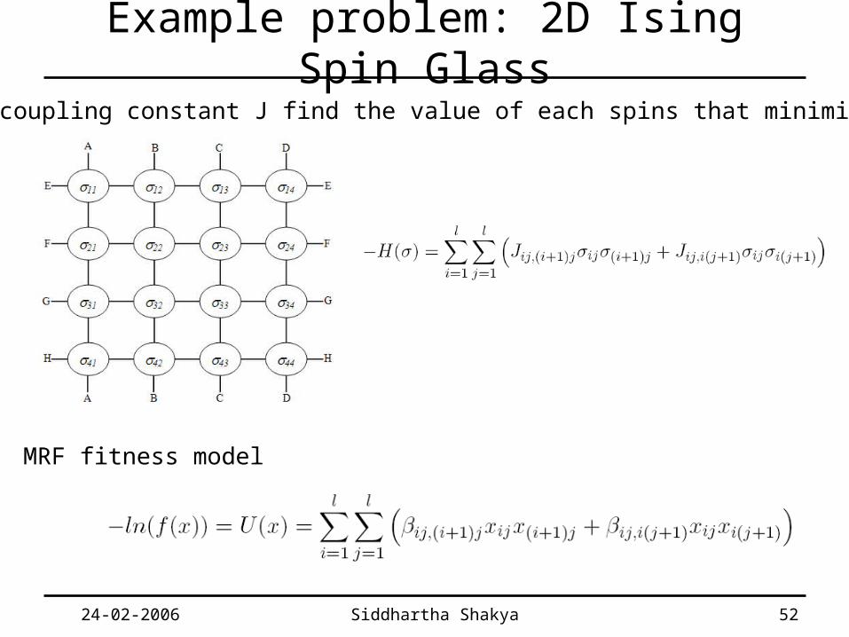
Example problem: 2D Ising Spin Glass
Given coupling constant J find the value of each spins that minimises H
MRF fitness model
24-02-2006 Siddhartha Shakya 53
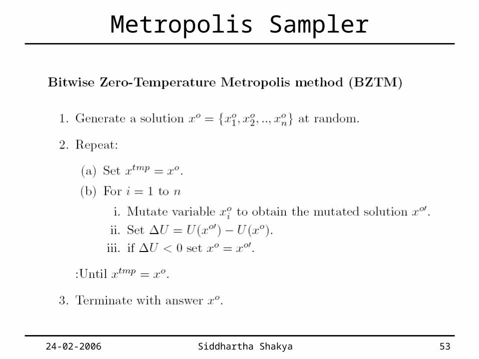
Metropolis Sampler

24-02-2006 Siddhartha Shakya 54
Difference in Energy

24-02-2006 Siddhartha Shakya 55
DEUM with Metropolis sampler
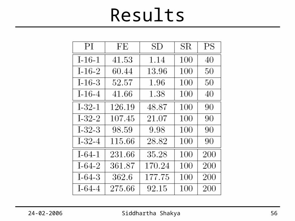
24-02-2006 Siddhartha Shakya 56
Results
24-02-2006 Siddhartha Shakya 57
Sampling MRF• Probability vector approach
• Direct Sampling of Gibbs Distribution
• Metropolis sampling
• Gibbs sampling

24-02-2006 Siddhartha Shakya 58
Conditionals from Gibbs distribution
For 2D Ising spin glass problem:
24-02-2006 Siddhartha Shakya 59
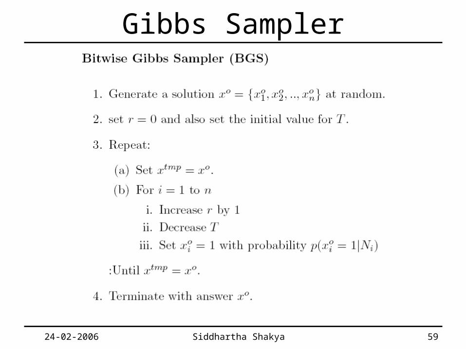
Gibbs Sampler
24-02-2006 Siddhartha Shakya 60
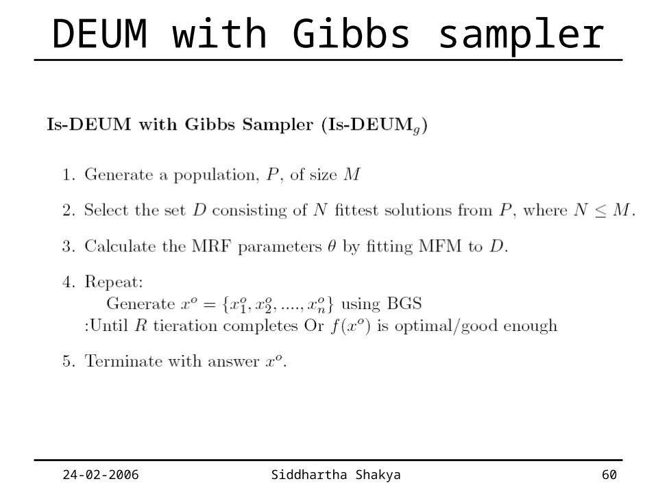
DEUM with Gibbs sampler
24-02-2006 Siddhartha Shakya 61
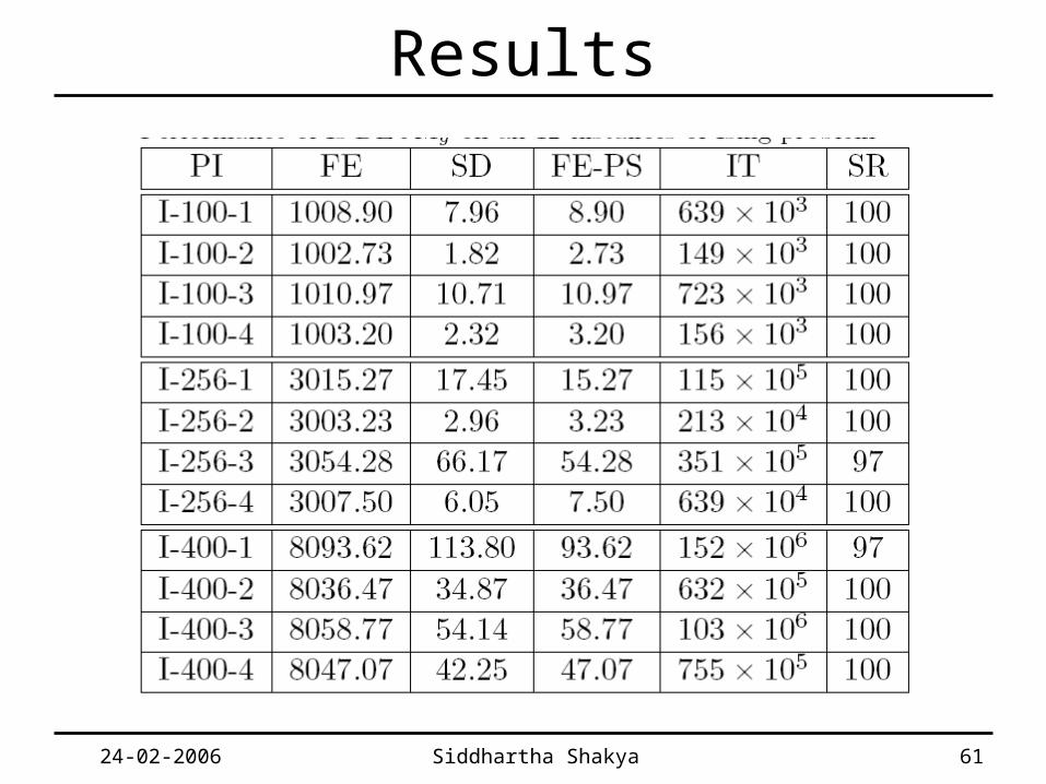
Results
24-02-2006 Siddhartha Shakya 62
Summary• From GA to EDA
• PGM approach to modelling and sampling distribution in EDA
• DEUM: MRF approach to modelling and sampling
• Learn Structure: No structure learning so far (Fixed models are used)
• Learn Parameter: Fitness modelling approach
• Sample MRF: – Probability vector approach to sample
– Direct sampling of Gibbs distribution
– Metropolis sampler
– Gibbs Sampler
• Results are encouraging and lot more to explore


![The Finall Water Shakya&Alex[1]](https://img.pdfslide.us/doc/110x75/5455150aaf795974408b514b/the-finall-water-shakyaalex1.jpg)